joint investigation of astronomical viewing · sao/nasa joint investigation of astronomical viewing...

SAO/NASAJOINT INVESTIGATION OFASTRONOMICAL VIEWINGQUALITY AT MT. HOPKINS -&-

OBSERVATORY: 1969-19710:, C -n c

M. R. PEARLMAN, J. L. BUFTON, D. HOGAN, " "

01 rD. KURTENBACH, and K. GOODWIN -

s ** * * . - t

is C1 rs L

;.,4

11- .o -

-*, * *. . ... .L .

-., 0ta. - . . ". " . .... .... .' '

-Smithsonian Astrophysical Observatory

https://ntrs.nasa.gov/search.jsp?R=19740013319 2019-02-10T03:37:37+00:00Z

TABLE OF CONTENTS

Page

ABSTRACT ...... .... ................... ........... ix

1 INTRODUCTION...................................... 1

2 THEORETICAL BACKGROUND AND EXPERIMENT RATIONALE .... 3

2. 1 Relationship of Atmospheric Turbulence to Optical Effects ..... 3

2.2 Scintillation ........................... .......... 7

2.3 Image Motion ................................... 10

2.4 Image Blurring........ ............... .......... 11

2. 5 Turbulence Profiles and Relationship of Meteorology to Turbu-lence Structure ........ _ ...... ............. .......... . 13

3 EXPERIMENT APPARATUS AND SITE LOCATION ............. 23

3.1 Stellar-Image Monitor System ............ .. .......... . 23

3.2 Temperature-Fluctuation Measurement System.............. 26

3.3 Temperature-Difference Measurement System .............. 27

3.4 Radiosonde ................... ............... 27

3. 5 Mt. Hopkins Observatory Site and Location of Experiment Equip-ment ........................ .................. 28

4 IMAGE-QUALITY MEASUREMENTS ...................... 33

4.1 Introduction .................................... 33

4.2 Image Motion ............................ ......... 34

4.3 Scintillation ................................... 45

5 CORRELATION OF IMAGE QUALITY WITH METEOROLOGICALPARAMETERS. . . ......................... .... ....... 57

5. 1 Image Quality vs. Local Meteorological Conditions .......... 57

5.2 Image Motion vs. Temperature Fluctuations. ............ 57

5.3 Image Motion vs. Temperature Gradient ................. 60

5.4 Scintillation Spectral Density vs. High-Altitude Winds ........ 64

5. 5 Image Motion vs. Temperature and Wind Profiles. .......... 66

PPECEDING PAGE BLANK NOT FILMED

TABLE OF CONTENTS (Cont.)

Page

6 COMMENTS AND APPLICATIONS........................... 69

6. 1 Comments on the Seeing Conditions at the Mt. Hopkins Site.... . 69

6.2 Comments on Site Testing ...................... . .... 71

6. 3 Direct Detection of Pulsed Laser Radiation . .............. 73

6.4 Heterodyne Detection of Continuous-Wave Laser Radiation ..... 76

7 ACKNOWLEDGMENTS ................................. 79

8 REFERENCES...................................... 81

APPENDIX A: COLLECTION AND REDUCTION OF SIM DATA A-i

APPENDIX B: DATA B-1

APPENDIX C: COMMENTS ON CORRELATION ANALYSIS C-i

iv

ILLUSTRATIONS

Page

1 Model of turbulent profile (Hufnagel, 1966b) .................. 15

2 The dimensionless temperature-structure parameter f 3 (Ri) versus theRichardson number R. (Wyngaard et al., 1971) ............... 20

1

3 Optical system and detector package for the stellar-image monitor. .. 24

4 Mt. Hopkins ridge and peak areas shown with access road. ........ 29

5 View of knoll 2 from the south ............................ 30

6 Detailed diagram of the ridge area showing the location of the equip-ment .................. ................... ....... 30

7 Cumulative probability distribution of one-dimensional image motionfor short-term averages during Phase I. The values have been cor-rected to zenith ..................................... 36

8 Cumulative probability distribution of one-dimensional image motionfor nightly averages during Phase I. The values have been correctedto zenith .......................................... 37

9 Three examples of short-term variations in ,m from Phase II datacorrected to zenith ................................... 38

10 Cumulative probability distribution of one-dimensional image motionfor short-term averages during Phase II. The values have been cor-rected to zenith ..................................... 40

11 Cumulative probability distribution of one-dimensional image motionfor long-term averages during Phase II. The values have been cor-rected to zenith ..................................... 41

12 Experimental dependence of T, on zenith angle. The sec 1/2() lineis intended to show the anticipated trend. Its intercept was chosenfor convenience only .................................. 42

13 Typical image-motion spectral density with 8-Hz noise componentintroduced by the SIM equipment ......................... 44

14 Cumulative probability distribution of CIV for short-term averagesduring Phase I. The values have been corrected to zenith ......... 46

15 Cumulative probability distribution of CIV for long-term averagesduring Phase I. The values have been corrected to zenith. ........ 47

16 Two examples of short-term variations in CIV. The values have beencorrected to zenith ................................... 49

17 Cumulative probability distribution of CIV for short-term averagesduring Phase II. The values have been corrected to zenith ........ 51

v

ILLUSTRATIONS (Cont.)

Page

18 Cumulative probability distribution of CIV for long-term averagesduring Phase II. The values have been corrected to zenith ........ 52

19 Experimental dependence of CIV on zenith angle. The secl14 (6) lineis intended to show the anticipated trend. Its intercept was chosenfor convenience only.................................. 54

20 Three examples of the normalized spectral density for CIV showingnoise contribution at 8 Hz from the SIM equipment .............. 55

21 Long-term-averaged image-motion and peak temperature fluctuationas a function of observation period during Phase II. The data fromobservation periods 6 and 27 were not available owing to equipmentfailure ........................................... 59

22 Long-term-averaged image-motion and temperature differences as afunction of observation period during Phase II................. 61

23 Probability of error in the presence of log-normal fading (Tittertonand Speck, 1973) .................................... 75

C1 Example of data distribution with corresponding correlation coeffi-cients ............................................ C-4

C2 Example of data distribution with corresponding correlation coeffi-cients ........................................... C-5

C3 Example of data distribution with corresponding correlation coeffi-cients ............................................ C-6

vi

TABLES

Page

1 Summary of rms one-dimensional image-motion statistics inPhase I..... ....................................... .. 34

2 Summary of rms one-dimensional image-motion statistics inPhase II ............................................. 43

3 Summary of scintillation statistics for Phase I .............. 48

4 Summary of scintillation statistics for Phase II............... 50

5 Correlation of rms image motion with average peak temperature

fluctuation in Phase II .................................. 58

6 Correlation of rms image motion with temperature difference(AT) in Phase II ............................................. 63

7 Correlation of scintillation half-width frequency with wind speed/correlation distance ratio (Phase II) ............... ....... 65

8 Scintillation: Power spectrum components vs. high-altitudewinds ......................................... 66

vii

ABSTRACT

Quantitative measurements of the astronomical seeing conditions have been made

with a stellar-image monitor system at the Mt. Hopkins Observatory in Arizona.

The results of this joint SAO-NASA experiment indicate that for a 15-cm-diameter

telescope, image motion is typically 1 arcsec or less and that intensity fluctuations

due to scintillation have a coefficient of irradiance variance of less than 0. 12 on the

average.

Correlations between seeing quality and local meteorological conditions are

investigated. Local temperature fluctuations and temperature gradients were found

to be indicators of image-motion conditions, while high-altitude-wind conditions were

shown to be somewhat correlated with scintillation-spectrum bandwidth.

The theoretical basis for the relationship of atmospheric turbulence to optical

effects is discussed in some detail, along with a description of the equipment used in

the experiment. General site-testing comments and applications of the seeing-test

results are also included.

PRECEDING PAGE BLANK NOT FILMIFa

ix

RESUME

Les mesures quantitatives des conditions astronomiques de visibilit6 ont td

prises ' l'observatoire du Mont Hopkins, en Arizona, A l'aide d'un systhme de

contrsle d'image stellaire. Les r6sultats de cette experience commune du SAO

et de la NASA indiquent que, pour un t6l6scope de 15 cm de diambtre, le mouve-

ment typique de I'image est de 1 seconde d'arc maximum et que les fluctuations

d'intensite dues ' la scintillation ont un coefficient de variation d'irradience

inferieur, en moyenne, ' 0,12.

On 6tudie les corr1lations qui existent entre la qualit6 de visibilit6 et

les conditions metiorologiques locales. On a trouv6 que les fluctuations de

temperature locale et les gradients de temp&rature indiquaient les conditions

de mouvement de l'image, alors que les conditions de vent en haute altitude

6taient, dans une certaine mesure, correlatifs de la largeur de bande du spectre

de scintillation.

On discute, de faon assez detaill6e, le fondement theorique du rapport entre

la turbulence atmospherique et les effets optiques, et l'on decrit le materiel

utilis6 pour l'exp~rience. Sont 4galement inclus, des commentaires generaux

relatifs aux essais sur place et aux applications des r6sultats de l'essai de

visibilite.

X

KOHCHEKT

SbIRZ EPOBegeHbJ KOJIMLieCTBeH[ibie z3mepeHi-ig aCTPOHOMZqeCKHX

YCJIOBZfi BM4MMOCTZ EOJIb3YRCB MOHZTOPOM 3Be3 4HCFO M3o6pa)KeHzF

B ObCePBaTopmz MaYHT rOEKMHC B Apm3OHe. Pecyi-if:,,iaTbT 3TOr'O

3KcEepmmeHTa COBmeCTHO nPOBeZeHHOFO CMZTCOHzaHCKOi ACTPO-

4)H3ztieCKOf ObcePBaTOpme2 z lJauliOHajiEHbIM KOMZTeTOM Eo acTpo-

HaBTm(e z iicc.TieZOBaHHf() KOcmi-iT4ecKoFo FIPOCTpaHCTBa, YKa3h!BalOT

T41 0 15 CNI TejieCKOria, ZBz)KeHiie H3o(fpa)KeHl-IR TPHIMLIHO RBJIFeTcyl

1 aPK-ceK Hqz meHBiiie ii 'qT(.) (1)TIYKTyauzm ZHTeHCI-TBHOC'1'1,1 BIDl31)IBa.em1)ie

mep4aHmem isiel'JT KO :(j)$i4uzeHT zzciiepcmm jiy,4ezclKYCKaHI-IH B cpezHem

k4eHbme 0. 1 I,-

liccj,,eZYIOTC.q KoppeRRuEz me)y4y KaLieCTBONI BHZZYO(-. Tll z MeCTHbIyli l

meTeopojiorztieCKMflA YCJIOBPiFMH. MeCTHbie KoTte6aHI-1,9 TemrlepaTYPLI

H rpazHeHThl TemnepaTYPLI bbIJIZ Ha2daeHht KaK YKa-qaTejji YCJITOBZ2

,gBmxeHMR M3obpax6HMf .. B TO BpeMH KaK BeTPOBbie YCU10BER Fa

bOJIbaIO2 BbICOTe 6bIJIM EOKa3aHbI B HeKOTOPOP ca eEeHVI COO TB eTCTBYDII ZMH

C MIIPHHO l nojioci-i crieKTpa iviepLiaHZq.

06cy)Kza.PJTCE ZOBOJIBHO geTajibHO., TeopeTlltiecKaR OCHOBa CBJq3Z

aTNIOccDePHO l Typby.7ieHTHCCTM C ORTHqeCKHMPI 3$(teKTam . OZHOBpelvieHHO

c onmcaHvem ObOPYZOBa im mcnojib3yemoFO B OnbITe. TaK)Ke BK.Tlm4eHbl

o6a ze 3ameT4aHMq 0 MCrIbITaHZRX CTaHUffi Z nPMMPH.FemoCTPf pe3yjiE)TaTOB

ZCDhTTaHffi BZ; ZMOCTH.

xi

SAO/NASA JOINT INVESTIGATION OF ASTRONOMICAL

VIEWING QUALITY AT MT. HOPKINS OBSERVATORY:

1969- 1971

M. R. Pearlman, J. L. Bufton, D. Hogan, D. Kurtenbach, and K. Goodwin

1. INTRODUCTION

During the period of June 1969 to February 1971, a series of experiments was

performed, under sponsorship of the National Aeronautics and Space Administration

(NASA) Headquarters, by the Smithsonian Astrophysical Observatory (SAO) at its Mt.

Hopkins Observatory. The purpose was to obtain quantitative information on the

astronomical "seeing" characteristics of the Mt. Hopkins site for future NASA and

SAO use and, if possible, to relate these characteristics to local meteorological

parameters. Data on nighttime stellar-image motion and scintillation were obtained

with a stellar-image-monitor system supplied by NASA Goddard Space Flight Center

(GSFC). Temperature-fluctuation measurements were made with a sensing device

supplied by the Jet Propulsion Laboratory (JPL). Local measurements of tempera-

ture, temperature gradients, humidity, and wind velocity and direction were made

and radiosonde data recorded on site. The analysis of the data was carried out jointly

by SAO and NASA.

The series of experiments were divided into two phases. In Phase I, the specific

goal was to monitor almost daily the astronomical seeing characteristics of the Mt.

Hopkins site for a long period of time. Stellar data were taken three nights a week.

Data collection began during June 1969 and continued until April 1970 except during

July and August. The stellar data from Phase I were compared with gross meteoro-

logical data. Because of a lack of any strong correlations between seeing conditions

This work was supported in part by gi AS 12-2129 from the National Aeronauticsand Space Administration.

Goddard Space Flight Center, Laser Technology Branch, Code 723.

1

and meteorological data, plans for Phase II were modified to include longer stellar

data runs on fewer observing nights and increased use of simultaneously acquired

meteorological and temperature-fluctuation measurements. The JPL measurements

of thermal fluctuation were begun in October 1970 and were employed to good advantage

during the second phase, which extended from September 1970 to February 1971.

The results of the experiments indicate that the seeing conditions at the Mt. Hopkins

Observatory are better than 1 arcsec on the average and that intensity fluctuations due

to scintillation have a coefficient of irradiance variance (CIV) of less than 0. 12 on

the average. We find very little correlation with gross meteorological conditions such

as temperature, humidity, and wind at the site. However, we find that local tempera-

ture fluctuations and temperature gradients are indicators of image-motion conditions

and that mild correlations exist between scintillation-spectrum bandwidth and high-

altitude winds.

We feel that our quantitative results and experience in comparing stellar-image

data and local meteorological indicators should be of interest to investigators who are

planning future programs at the Mt. Hopkins site and to those who, in general, are

concerned with characterizing optical propagation effects on the vertical path at any

other site. In particular, data of this type can be used to estimate the atmospheric

channel performance for both coherent and pulsed-laser communication systems of

high data rate. A discussion of these applications is included in this report.

2

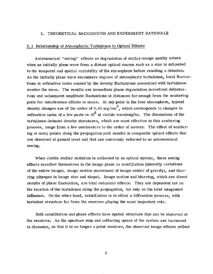
2. THEORETICAL BACKGROUND AND EXPERIMENT RATIONALE

2. 1 Relationship of Atmospheric Turbulence to Optical Effects

Astronomical "seeing" effects or degradation of stellar-image quality arises

when an initially plane wave from a distant optical source such as a star is subjected

to the temporal and spatial variability of the atmosphere before reaching a detector.

As the initially plane wave encounters regions of atmospheric turbulence, local fluctua-

tions in refractive index caused by the density fluctuations associated with turbulence

scatter the wave. The results are immediate phase degradation (wavefront deforma-

tion) and subsequent amplitude fluctuations at distances far enough from the scattering

point for interference effects to occur. At any point in the free atmosphere, typical

density changes are of the order of 0. 01 mg/cm3 , which corresponds to changes in

refractive index of a few parts in 106 at visible wavelengths. The dimensions of the

turbulence-induced density structures, which are most effective in this scattering

process, range from a few centimeters to the order of meters. The effect of scatter-

ing at many points along the propagation path results in composite optical effects that

are observed at ground level and that are commonly referred to as astronomical

seeing.

When visible stellar radiation is collected by an optical system, these seeing

effects manifest themselves in the image plane as scintillation (intensity variations

of the entire image), image motion (movement of image center of gravity), and blur-

ring (changes in image size and shape). Image motion and blurring, which are direct

results of phase fluctuation, are total columnar effects. They are dependent not on

the location of the turbulence along the propagation, but only on the total integrated

influence. On the other hand, scintillation is in effect a diffraction process, with

turbulent structure far from the receiver playing the most important role.

Both scintillation and phase effects have spatial structure that can be observed at

the receiver. As the aperture stop and collecting optics of the system are increased

in diameter, so that it is no longer a point receiver, the observed image effects reflect

3

a spatial averaging of the starlight phase and irradiance pattern sampled by the aper-

ture. The magnitude of scintillation decreases with increasing aperture. When the

aperture diameter exceeds the correlation length of the irradiance structure (8 to

10 cm), dictated by atmosphere quality and observation geometry, the effects of scin-

tillation are significantly reduced. For small apertures, the dominant effect of the

phase structure sampled is image motion, which is a result of the entire incident

wavefront being tilted. As aperture diameter is increased, tilts in various regions

of the aperture become uncorrelated, and the image undergoes more complex

changes in size and shape, which lead to blurring. Aperture diameter common to

stellar astronomy are in the range of 1 to 2 m, where scintillation effects are quite

small; and the most serious degradation of image resolution is blurring rather than

image motion. For convenience and economy of operation, we used a relatively

small optical system (15-cm-diameter refractor) to facilitate the measurement of

scintillation for our stellar-image data measurement. In our experiment, the pri-

mary phase-structure effect was image motion. Accordingly, the following discus-

sions will primarily treat scintillation and image motion; however, some discussion

on image blurring and the effects at large telescope diameters will also be included.

The turbulence process in the atmosphere is quite random in nature and thus

produces an ensemble of spatial and temporal fluctuations for the observed optical

effects. Accordingly, any description of this process must be statistical. For most

situations that occur in the free atmosphere, the turbulence process itself has been

found to be locally stationary, homogeneous, and isotropic; here, locally refers to

that region of space and time for which the description of turbulence remains the same.

Within each locality, an inertial subrange of turbulence-element sizes is said to exist.

The inertial subrange is bounded on the upper end by an "outer scale, " whose dimen-

sions are characteristic of those processes responsible for the flow of energy into the

turbulence process. The minimum or "inner scale" is dictated by the processes in

which turbulence energy is dissipated as viscous friction. Energy is input to the

system as turbulence of large scale and cascades down adiabatically to form the inertial

subrange. The difference from one locality to another is simply the strength of tur-

bulence, or scale factor, that multiplies the description of the inertial subrange. In

addition to changes with time (nonstationarity), the nature of the atmospheric turbulence

4

changes significantly with altitude above the Earth's surface, but only moderately

with horizontal displacements through the atmosphere. An overly simplified model of

turbulence distribution would be a series of horizontal slabs or strata of well-developed

turbulence slowly changing in time and interspersed with calm air.

The widely accepted Obukhov-Kolmogorov turbulence theory (Obukhov, 1941) states

that within each inertial subrange, the spatial distribution of turbulence sizes and

related physical properties obey identical power-law descriptions. The structure func-

tion, i. e., the mean-square difference of a quality of the turbulence, such as refractive

index between two points as a function of the separation of the points (rl, r 2 ), is a com-

plete statistical description. For visible radiation, temperature is the most important

property that affects refractive index. The velocity fluctuations of turbulence cause

temperature fluctuations as cold and warm parcels of air are mixed. Since the atmos-

phere will not support local pressure gradients, density and thus refractive-index

fluctuations follow directly from the temperature fluctuations. The Obukhov-Kolmogorov

theory expresses the temperature-structure function,

2 2 r2/3Dw(r) ([T( 2) - T(r 1)]2)= CT r (1)

for i << r = r2 - r o, where T(r) = ambient temperature at point r, r = spatial

separation, I. = inner scale, 10 = outer scale, and CT is temperature-structure

coefficient, a strength factor for the temperature fluctuations. From one locality to

another, C changes but the r 2 / 3 dependence remains. The inner scale, Ii, is about

1 cm near ground level and is thought to increase slowly to about 10 cm at 10-km

altitude. The outer scale, , has been estimated to be roughly equal to height above

ground for the near-Earth environment and to be on the order of about 1 km at high

altitude. For the narrow, nearly vertical propagation path that we are concerned with,2

the important variations in CT are with altitude above ground and with time. The

dependence on altitude h will be denoted here as CT(h), and it will be understood that

the coefficient value applies to a particular time or time average of a measurement.

The effect of temperature fluctuations (of strength C2(h)) on refractive index is

obtained by a straightforward application of the general formula (U. S. Air Force

Research Center, 1960) for refractive index and the ideal gas law. The result for

radiation in the visible or near infrared is given by

5

C2 (h)[= 80P(h X 10-62 C2(h) (2)T (h)C

where P is the atmospheric pressure (mb), T is the temperature (K), and C2(h) is

the strength factor or the refractive-index-structure coefficient. This is the desired

connecting link between turbulence strength and optical refractive-index effects. It is

now necessary to express the observed optical effects of scintillation and image motion

in terms of C (h), and for this, we must turn to wave-propagation theory.

Many theoretical treatments have addressed the problem of optical wave propaga-

tion through a turbulent medium. The most successful of these have relied on approxi-

mate solutions to the scalar wave equation,

V2 U(r) + k2 N(r) U(r)= 0 , (3)

with U(r) = wavefunction (electromagnetic wave), k = 2r/kX, the free-space wavenumber,

and N(r) = index of refraction. For a stellar source, the incident, normalized plane

wave can be represented as

U(r) = A(r) exp [ikc(r)] = exp Ek( + loge ()] , (4)

with A(r) = amplitude and 4((r) = phase. As a wave propagates toward Earth, it is

perturbed by the turbulence in a multiplicative manner. As a result, quantities in the

exponent add; and, after scattering from many points in the turbulence field, a gaussian

distribution is implied by the central limit theorem for ( and loge (A/A 0 ). This

property has aided the calculation of statistical quantities dependent on phase and

amplitude. The "Rytov approximation" has been used by Tatarski (1961) and others to

linearize the wave equation by neglecting small terms in the plane-wave formulation

of the scalar wave. This theoretical development is widely accepted for weakly scat-

tered fields. For strong scattering, often observed over horizontal near-ground

propagation paths in the daytime, a scattering saturation effect not predicted by the

theory is observed. For the case here, i. e., near-vertical paths at night, no satura-

tion effects are observed and the theory is thought to be valid. Where appropriate

6

below, the Rytov solutions for the statistical quantities necessary to explain scintilla-

tion and image motion will be quoted.

2.2 Scintillation

Total image intensity and the resulting fluctuations (i. e., scintillation) result from

the irradiance pattern of starlight sampled by the telescope aperture. Irradiance varies

with both position and time in the aperture plane. As noted above, the quantity log

amplitude [loge(A/AO)] should obey gaussian statistics. Log amplitude can be defined

in terms of irradiance,

loge () 1(x, t) = -loge (x, t) (5)

where l (x, t) is instantaneous log amplitude at point x in the aperture plane, I(x, t) is

corresponding irradiance, and I0 is average irradiance. An expression for log-

amplitude variance, a2, follows (Tatarski, 1961, chapter 13) from the Rytov formula-

tion and the Obukhov-Kolmogorov turbulence theory:

00

k7/6 11/6 2 5/6a = 0. 56 k sec 0 C (h) h dh , (6)

0

where k = 2rr/X and 0 = stellar zenith angle. This equation is valid for a point detec-

tor - i.e., a telescope with aperture small enough so that the instantaneous irradiance

is everywhere constant within the aperture. The wavelength dependence, k7/6 , pre-2 2dicts that 0 is reduced by 20% in passing from 0.45 pm to 0. 55 pm. While or is

reduced in magnitude at the higher wavelength, analysis (Tatarski, 1971) has shown

that spectral correlation of a remains high for this separation of wavelengths. The

angular dependence in a, reflects the h5 / 6 weighting and the air mass through which

starlight must pass before reaching the telescope. This angular dependence breaks

down for large zenith angles owing to the increased role of chromatic dispersion and

to the resultant multipath effects through spatially uncorrelated turbulence. The2

dependence of o on the strength of turbulence involves the 5/6 moment of altitude,showing the strong influence of even relatively low turbulence at high altitudes and the

deemphasis of high turbulence conditions near the surface.

7

A photomultiplier tube or other square-law device is normally used in field work

to obtain data on the stellar image. Electric-current output from this device is pro-

portional to irradiance, not amplitude; and it is sometimes more convenient to handle

the data in terms of irradiance statistics. The ratio of rms image-intensity fluctua-

tions to the average value is a fundamental measure of irradiance statistics, called

the coefficient of irradiance variance:

CIV = r/I 0 , (7)

where or2 = irradiance variance = (I- I0)2). The connection with log-amplitude

statistics is

CIV2 2 2CIV exp (40) - 1 4 (8)

where the approximation holds for the typically observed values of 2 much less than 1.

The time structure of the irradiance pattern is best described by the autocorrela-

tion function and its Fourier transform - i. e., the spectral-density function. Typical

frequency content of scintillation is of the low-pass filter type extending from dc to

frequencies of several hundred Hertz. The bandwidth of these spectra can be specified

as the frequency value at which the spectral density function has fallen to 50% or,

alternately, 10% of its maximum value. The bandwidth and, indeed, the shape of each

spectrum are tied directly to the components VN(h) (component of mean horizontal wind

speed V (h), which carries the existing turbulence perpendicular to the line of sight).

The quantity VN(h) can be computed from Vo(h) with the additional knowledge of stellar

zenith angle 0, azimuth angle a, and mean wind direction P (see Young, 1969),

Vo(h) 2 1/2VN(h) = sec [1 + tan 6 sin2 (a- )] . (9)

The size of the turbulence elements at each altitude that are most effective in contri-

buting to scintillation is given by Fresnel diffraction theory as ATh sec 0. Thus, the

frequency at which each layer of wind speed is most effective in contributing to

irradiance spectral density is proportional to

8

VN (h) (10)vXh sec e

From this proportionality, it can be seen, for instance, that very low frequencies of

scintillation should be associated with low wind speed at high altitude. Alternately,

high wind speed and lower altitude contribure more to the high frequencies of scintilla-

tion. Modest correlations were found in our experiments between CIV spectral band-

widths and wind speeds at selected altitudes.

As the telescope aperture is increased in diameter from the point detector neces-2

sary for equation (6) to hold, the strength of scintillation, measured either by a or

by CIV, decreases rapidly at first and then more slowly as the spatial correlation

distance of irradiance in the aperture plane is exceeded. For large apertures, the

scintillation bandwidth is decreased while dependence on zenith angle to the star is

increased. The spatial correlation distance of irradiance is determined by noting the

separation distance at which the correlation between scintillation observed by two point

detectors falls to 1/e of that observed at zero separation. Once again, by use of

Fresnel diffraction theory, this distance can be associated with an altitude h0 that is

most effective in producing the strongest scintillations,

spatial correlation distance = V h sec 0 . (11)

Experimental values for correlation distance are typically 8 to 10 cm for zenith view-

ing. For values of X in the visible region, h is on the order of 10 to 20 kin, where

we expect significant turbulence due to the favorable meteorology of the tropopause

and jet stream. This is additional evidence linking scintillation effects to turbulence

at high altitude.

There are several theories for prediction of aperture-averaging effects for

scintillation. They all result in a functional dependence on aperture diameter, correla-

tion distance, and or for a point detector. Unfortunately, at present no one theory can

explain all the observed effects, especially for apertures larger than 1 m in diameter.

Tatarski (1961) develops a general expression for aperture dependence that relies

explicitly on the correlation coefficient of the fluctuations in log amplitude. Assuming

9

a case where C is constant, he shows that the log-amplitude variance, and thusn -7/3

CIV depends on aperture D through the relation (D/--L) / 3 . With arguments

from geometric optics, Reiger (1963) finds a similar dependence on aperture for

scintillation.

Experimental work by Protheroe (1954), Tatarski (1961, 1971), and others shows

the CIV or o zenith-angle dependence to vary with aperture as:

aperture diameter dependence

3 in. (sec 9) 0 . 9

6 in. (sec ) 1.2

12.5 in. (sec ) 1.4

Protheroe's data have been used to develop the following equation for a 15-cm (6-in.)

aperture:

o00

S/(15 cm)= 0.09k7/6 sec2.4 f C(h) h5/6 dh . (12)

0

The CIV data taken in this experiment at Mt. Hopkins with a 6-in. telescope agree

well with the (sec 0) 1. 2 dependence observed by the above investigators.

2.3 Image Motion

Movement of the image center of gravity results from a linear phase change or

tilt in the incoming wavefront. In the limit of a point detector, all phase changes

appear linear. For a finite aperture, however, phase changes in different parts of

the aperture become more uncorrelated as aperture diameter increases. Any image

motion is then due to a resultant tilt after spatial averaging in the aperture plane.

The uncorrelated phase changes also result in blurring of the image.

An expression for image-motion variance am (in square radians) can be derived

by the Rytov method of Tatarski (1961), the Obukhov-Kolmogorov turbulence spectrum,

and the modifications by Hufnagel (1966a) to include a circular aperture. The result,

10

o = 0. 56 D-1/3 see C2(h) dh , (13)

0

is independent of wavelength and applies only to motion in one dimension of the image

plane. Under the assumption of isotropic image motion, the total two-dimensional2 -1/3

image-motion variance is 2a . The aperture diameter dependence D- /3 is weak;m 2

only a decrease of a factor of 2 in o2 is predicted when D increases by a factor of

10. The dependence on air mass (sec 0) is linear, and the dependence of turbulence

strength is a straightforward integration over C (h) along the propagation path. It

should be noted that equation (13) depends on theory that is valid only for

D > A h see 0, the irradiance correlation coefficient. For smaller apertures, the-1/3 o

D 1/3 dependence holds but the constant multiplier will be reduced. In addition, the

inner and outer bounds on D, for which (13) applies, are determined by the inner iiand outer 1o turbulence scale sizes, respectively, which, as noted before, vary with

altitude and with time. With these factors and limitations in mind, equation (13) should

be an adequate prediction for the one-dimensional motion measured by the 15-cm-

diameter telescope used in this experimental study. Data taken by Kolchinskii (1969)

and in this experiment at Mt. Hopkins show a zenith-angle dependence that agrees well

with this relation.

Several theoretical treatments based on different approximations for the spectral

density of image motion have resulted in expressions involving the normal wind com-

ponent VN(h) and turbulence strength C2(h). Observed spectra indicate extremely

low-frequency behavior for image motion. Most energy is contained below 5 Hz, with

typically less than 1% of the motion above 20 Hz. To predict such low frequencies,

the theoretical treatments require low wind velocities of only a few meters per second.

These velocities generally occur at ground level or above 20 km. Since image motion

is equally weighted to all regions of turbulence depending only on the value of C (h)nand since owing to the rarefied air, little turbulence is expected above 20 km, the

implication is that image motion is associated with turbulence near ground level.

2.4 Image Blurring

Specification of image size or profile is the final step in a description of the

atmospherically distorted stellar image. Size determination and the whole investigation

11

of image quality are handled easily through the use of optical transfer-function tech-

niques. The modulation transfer function (MTF) of an optical system is a measure of

reduction in contrast suffered by each Fourier component of the object after trans-

mission through the entire imaging system. It is a function of a transform variable,

the image-plane spatial frequency f. The variable f has dimensions of cycles per unit

length. Multiplication by system focal length allows spatial frequency to be expressed

in cycles per radian of the field of view. This will be denoted as W and is easily

related to cycles per second of arc.

The image blurring to be expected in telescopes of aperture diameter greater

than 15 cm can be estimated from the MTF; all data reported here were obtained

with such telescopes. The observed MTF of M(w)o for starlight observations is the

product of the telescope MTF, which is M(w)T, and the atmospheric MTF, which is

M(w)A:

M(w)o= M(w)T M(w)A . (14a)

If the averaging time of the experimental determination of M(o)o is small, as it is in

short-exposure photography, all effects of image motion are frozen out. The resultant

image is sharper, differing from the diffraction-limited case by only the contribution

of residual atmospheric blur. Laboratory calibrations and field measurements at

Mt. Hopkins with the 15-cm telescope revealed little if any image degradation beyond

that already present in the telescope optics. This is essentially a restatement that

atmospherically induced phase degradation appears primarily as image motion in

telescopes of diameter 15 cm or smaller. The net result is that M(w)A for the short-

term time average can be approximated by unity. For long-term time averages, as

is the case in a long-exposure photograph or in an image viewed through a large-

diameter telescope, M(w)A becomes the product of the short-term atmospheric MTF

and an MTF constructed from image motion,

2

M(w)M = exp r2 2 , (14b)

12

as reported by Hufnagel (1966a). Although this result is constructed with m, or one-

dimensional image-motion variance observed through the aperture of 15-cm diameter,

it specifies the atmospheric contribution to long-term image degradation by virtue of

the short-term M(w)A being nearly unity for the 15-cm aperture. Image profile due to

atmospheric effects is obtained by applying the inverse Fourier transform,

o00

I(s) = 2 f wM(w)M Jo(2r sw) dw , (15)

0

where s is seconds of arc in the focal plane. Inserting equation (14) in equation (15)

and approximating the integral yields

I(s) = exp I . (16)

2

This is a gaussian shape with variance om . Thus, the rough estimate of image size

(diameter at half maximum) in a large telescope is just 2 am, where om is rms image

motion expressed in seconds of arc.

2. 5 Turbulence Profiles and Relationship of Meteorology to Turbulence Structure

The common factor in the foregoing wave-propagation theory is an integral

expression containing C n(h), the refractive-index structure constant as a function of

altitude. Lack of both experimental and theoretical knowledge of this profile is the

single greatest obstacle to full understanding of vertical propagation. If the profile

were known, optical-propagation theory could be tested in any number of interesting

experiments, and astronomical seeing could be predicted in advance. What experi-

mental data are available suggest that turbulence strength is usually greatest in the

first kilometer comprising the atmospheric boundary layer, with occasional but per-

sistent layers of secondary strength at high altitudes in the troposphere and lower

stratosphere. The near-ground turbulence is found to be quite dependent on local

terrain, local meteorology, and time of day, while the upper altitude structure is

more constant in time and space.

13

Data on boundary-layer turbulence have been reported by Coulman (1969), Tsvang

(1969), and Lawrence, Ochs, and Clifford (1970). These data were obtained by meas-

uring, from balloon and aircraft platforms, the profiles of microthermal statistics and

thus Cn(h). More recently, Bufton, Minott, Fitzmaurice, and Titterton (1972) extended

balloon-borne temperature-sensor measurements to the region of the tropopause. All

these investigators report wide fluctuations in C (h) and thus C2(h), which indicate

that the turbulence process is quite nonstationary. It is only with time averages on

the order of minutes that an average profile or envelope of the fluctuations of C (h) can

be constructed. The average profile can then be used effectively to predict optical

propagation effects. In the absence of other data, this consideration has lead several

researchers to construct a turbulence-profile model, i.e., a functional dependence

for the average behavior of CN(h). Model parameters can then be adjusted for correct

prediction of ground-based stellar data. A particularly useful model is that reported

by Hufnagel (1966b) and shown in Figure 1. His curve is for nighttime atmospheric

conditions; it exhibits a near-ground maximum of 2 X 10- 14 m - 2 / 3 , an exponential-like

decrease to 10- 17 m - 2 / 3 at 1000 m, a relatively constant range of minimum values

to about 10 km, and then a sharp bump of height 2 X 10- 16 m - 2 / 3 at 12 km. Brookner

(1971) describes this profile analytically as

CN(h ) = 2. 5 X 10- 1 3 h - -h / 3 2 0 + 2 X 10 6 (h - 12 Ikm) . (17)

The exponential decrease near ground level corresponds reasonably well to observed

CN(h) data, but the delta-function spike at 12 km does not. Actually, high-altitude

thermal-sensor data reported by Bufton et al. (1972) and extensive radar backscatter

measurements reported by Hardy and Katz (1969) reveal many thin, highly tur-

bulent layers distributed over the altitude range of 4 to 15 km. The delta-function

model has a magnitude equal to the integrated effect of these multiple layers and is

centered near the midpoint of their distribution; however, it does not have the correct

distribution for upper altitude turbulence.

Any model proposed should reflect probable meteorological factors at the origin

of turbulence. As noted previously, essentially all refractive-index variations are

accounted for by small-scale temperature fluctuations. These in turn can be related

to the pertinent larger scale meteorological parameters. The intent is not to construct

14

304-045

i0 - 1 2 1 i i 1 I i , l l I i I I ll ll I I- 13

13 -141.9 x 10 EXP (-h/3500)

-14 -1410 9.9 x 10 EXP

h 5 /3 (-h/lOO)

o -15 -13c1 \ 9.1 x 10 EXP

(-h/1000)E h 2 / 3

mz -16

- 1710

io-18

-1910I I I IIIi l I I I1I l I I 111111 I I I 11I

10 100 IK IOK

ALTITUDE (m)

Figure 1. Model of turbulent profile (Hufnagel, 1966b).

15

an actual profile from meteorological parameters but to show their influence and to

select for measurement those parameters that would provide a useful estimate of

turbulence conditions.

The strength of the turbulence along the observation path, or CT(h), is a measure

of the spatial fluctuations in the temperature field. In the presence of a wind field,

this spatial temperature structure is observed as temporal fluctuation at fixed refer-

ence points. The first obvious quantity to investigate, then, is temperature fluctua-

tion in the vicinity of the site and along the vertical observation column. From

equation (13), we expect a linear relation (correlation) between temperature fluctua-

tions and a m. Investigations using microthermal sensors near ground level have been

carried out by Coulman (1965) and others (Tsvang, 1969; Ochs, 1967). A sensing

device that measures the average value of the peak temperature fluctuations was used

with some success in the present experiment.

Another approach to explain seeing conditions in terms of meteorological

parameters is based on the connection between CT and the small-scale processes

involved in turbulence activity. From Tatarski (1961, chapter 10),

2 -1/3CT oc NE (18)

where N is the rate at which temperature variations in the atmosphere are dissipated

by molecular activity, and E is the analogous dissipation rate for turbulent kinetic

energy.

Numerous measurements of E are available for at least the lower altitudes.

Typical values, as quoted by Hufnagel and Stanley (1964), show a decrease from

300 cm2/sec 3 at ground level to 0. 07 cm2/sec 3 at 10 km and then an abrupt rise,

although the data for this region are scarce and quite inconsistent.

The quantities N and E can be expressed in terms of gradients of temperature and

wind velocity (Tatarski, 1961):

N(h) = D [L(h)J (19)

16

and

E (h)=KD ~U 2 (20)

where

O(h) = potential temperature (K) = T(h) - F,

T(h)= actual temperature (K) ,

F = adiabatic lapse rate, which is equal to -9.8 K/km

U(h) = mean wind speed,

D = coefficient of molecular diffusion, and

KD = coefficient of turbulent diffusion .

We then expect that gradients of temperature and wind velocity (shear) will be fruitful

quantities to investigate when we look for correlations with image motion.

The vertical gradient of the potential temperature, or the relationship betweenYT-h and 1, is in fact a measure of static thermal stability. In particular,

8T-h < F , unstable ,

aT6= 0 neutral ,

(21)8T > F , stable, and

aT- > 0 inversion

In the atmosphere at night, the temperature lapse rate is often inverted near the ground

and neutral or stable at higher altitudes. Values of a U/ah are the least well known.

As Hulett (1967) pointed out, small-scale shears between layers a few tens of meters

apart are not often included in the reported data. Yet shears of this dimension

probably have most influence on optical effects.

The three parameters of equations (18), (19), and (20) are height dependent and

also are functions of one another. Thus, it is difficult to isolate a single cause of tur-

bulence. Tatarski (1961) has shown, however, that C (h) can be expressed as

17

C (h) = L4/3 [ a (22)

where L is a measure of the outer scale of the turbulence. As noted previously, this

outer scale is roughly equal to the height above ground for regions near the surface

and is on the order of 1 km for higher altitudes.

For some specific cases, C2(h) has been determined analytically for at least the

boundary region near the ground.

Values of N, E, and hence C (h) in the atmospheric boundary layer are strongly

dependent on the atmosphere-terrain interaction. Tatarski (1961) and others have

looked at this region for the simplest case in which air moves in a flat plane. Under

the assumption that buoyancy forces are small (i. e., mean temperature varies slowly

with height), the wind velocity can be shown to vary logarithmically:

U(h) cc log (h/h ) , h >> h ,

where h0 is a scale length characteristic of terrain roughness. For ease of computa-

tion, Tatarski (1961) assumes a slowly varying temperature profile of the form

T(h) = T + T, log (h/h) ,

where T, is a logarithmic lapse rate assumed to be small compared to T . Using

arguments based on the Obukhov-Kolmogorov turbulence structure, Tatarski shows

that

2 2CT(h) c T 2

and that

T(hl) - T(h 2)CT(h) cc h1/3 , for h i < h2 (23)

h log (hl/h 2)

18

The proportionality has been checked experimentally by Tatarski, who finds that the

constant of proportionality is larger for stable conditions [T(hl) < T(h 2 )] than for

inversion conditions [T(hl) > T(h 2 )]. Even under an inversion condition typical of

nighttime, the near-Earth turbulence is dominant. Thus, there is good reason to look

for a correlation between stellar image motion and the mean temperature gradient,

with less image motion to be expected under inversion conditions. In our experiments

at Mt. Hopkins, we found fairly significant correlations between image-motion condi-

tions and temperature-difference measurements made in the vicinity of the observa-

tion site.

Recently, a more complete method to compute C (h) in the boundary layer has

been reported by Wyngaard, Izumi, and Collins (1971). Starting with equation (18),

they are able to show on a semiempirical basis, for conditions of a flat unobstructed

plain, that

-22 4/3 -a_ 2CT(h) h h f 3 (Ri) (24)

for the boundary layer, where R. is the Richardson number,

R. = g [a8(h)/ahl (25)T1 [86(h)/ah]

a widely used measure of stability, and f3 is a dimensionless temperature-structure

parameter, which is empirically determined by Ri alone, g is the acceleration of

gravity, and T is the mean temperature.

Values of R. near 0. 25 are considered necessary for turbulence onset, while

values up to 1.0 are permissible for ongoing turbulence. While small R. numbers are1

necessary, they are not sufficient for the development of turbulence. The most useful

role of R i is as an indicator of the presence of turbulence. The function f 3 (Ri)

was computed by Wyngaard et al. (1971) from their own data on boundary-layer tur-

bulence over a flat Kansas plain. Their result is dependent only on ambient tempera-

ture, on temperature gradient, and on Ri, the measure of stability. A graph of

f 3 (Ri) as a function of R i is included in Figure 2. There is no explicit dependence on

local parameters like surface roughness and wind speed, for these are all suppressed

19

10.0

o.-

0.1-

0.01 I I I-2.2 -2.0 -1.8 -1.6 -1.4 -12 -1.0 -0.8 -0.6 -0.4 -0.2 0 0.2 0.4

R

Figure 2. The dimensionless temperature-structure parameter f3 (Ri) versus theRichardson number Ri (Wyngaard et al., 1971).

20

in the formation of f (Ri). This method holds promise for a more accurate determina-

tion of C2(h) than does the technique relying on temperature gradient only; however, it

requires the additional measurement of wind shear, (aU/ah), for calculation of Ri.

Accurate wind-shear measurements are difficult to obtain because of uncertainties

associated with the spacing and resolution of wind sensors.

We used equation (18) to estimate C (h) values in the lowermost region along the

propagation. Temperature profiles were measured with radiosonde flights. Wind speeds

as a function of altitude were estimated from radiosonde-balloon positions. Even with

wind speed determined in this fairly crude manner, modest correlation coefficients

between the integral of CT(h) over the lowest 1000 m and a m were found.

Upper altitude turbulence can also often be identified by small Ri numbers. The

availability of wind shear seems to be the controlling factor for this region. Typically

high wind-shear values when squared in the denominator of the Ri number dominate

the weaker influence of the temperature lapse rates. In fact, high turbulence has

been found to associate with thin, stable, or even inverted temperature lapse-rate

layers. As Scorer (1969) and Roach (1970) have pointed out, thin stable layers are

especially suited for the development of turbulence when mechanisms exist to tilt them.

Suitable mechanisms could include pressure fronts, gravity waves, and mountain or

lee waves. At observatories located in mountainous regions, the mountain or lee wave

mechanism should almost always be present. It is also at these wave boundaries or

interfaces between air masses that the higher values of wind shear are found. Although

stable or inverted layers may be found at all altitudes, the tropopause is especially

suitable because of its large region of temperature stability. Once the stable layers

are tilted and the condition R. - 0. 25 is reached, the tilts develop into Kelvin-

Helmholtz rolls or billows, as illustrated by Roach (1970). Smaller, secondary

instabilities are formed, and the now well-developed turbulence feeds on available

wind shear to grow in extent. Turbulent energy cascades into smaller and smaller

eddy sizes, becoming more isotropic until it is lost in viscous dissipation at the inner

scale. Layer thickness may be only a few tens of meters, but horizontal extent is

usually on the order of kilometers. Thus, the same series of turbulence layers or

sheets should affect astronomical viewing at many different azimuths during the same

time period.

21

Because the upper altitude turbulence layers, though well developed, do not have

the strength of boundary-layer turbulence, optical-phase effects should have little

additional contribution from these layers. Scintillation effects, however, are strongly

weighted by altitude and thus should exhibit strong correlation with upper altitude

turbulence layers. In lieu of direct measurement, useful tracers or estimators for

the presence and strength of upper altitude turbulence should be the wind-shear squared

profile, inflections in the temperature lapse rate, and the presence and sharpness of

the tropopause region.

22

3. EXPERIMENT APPARATUS AND SITE LOCATION

3. 1 Stellar-Image Monitor System

Image motion and scintillation were measured with a Stellar-Image Monitor (SIM)

developed and built at GSFC during 1968. It was patterned directly on a technique

described by Lindberg (1954) and a design published by Ramsay and Kobler (1962).

Ramsay performed some experimental work with starlight. Later, Coulman (1969)

used the device extensively for studies of horizontal optical propagation. The hard-

ware of the Ramsay SIM produces three analog voltage signals containing information

on image intensity, size, and motion. These voltages can be analyzed for the desired

statistics on the stellar image. The heart of the device is an MTF measurement

performed by square-wave modulating or chopping the incoming light in the telescope

focal plane. Chopping is performed at a selected, but variable, spatial frequency.

Operation at various spatial frequencies, detection of the chopped light, and electronic

processing yield various points for an MTF that contains accessible information on

image blurring. Image intensity is monitored by low-pass filtering of the chopped signal.

Image-motion information is derived from electronic phase comparison of signals

generated in chopping the stellar image and a reference light source. The Goddard

device differs from the original Ramsay design in the way spatial frequency is varied,

in electronic processing, and in data collection and reduction.

Starlight is collected by an 0.152-m-diameter doublet lens system of 1.22-m focal

length. Figure 3 indicates the optical system components. A microscope objective

serves as relay optics to focus an enlarged image of a star on a rotating glass disk.

An eyepiece and mirror assembly mounted in a sliding tube are used to check visually

the image quality and to ensure proper alignment of the image on the glass disk. The

disk is composed of alternately clear and opaque pie-shaped sectors, each subtending

0. 5. The disk is belt-driven from a dc motor servosystem at a constant rate of

500 rpm. Speed regulation is better than 0. 5%. Light passing through the disk is

square-wave-modulated with a frequency of 3. 0 kHz determined by the motor speed

23

304-045

OPTICALSLIDING HIGH-PASS

EYEPIECEMICROSCOPE FILTER

WIDE-FIELD OBJECTIVEFINDER SCOPE PHOTOMULTIPLIER

/ TUBE

MIRROR

6-INCHf/8 LENS BEAMSPLITTER

NARROW-FIELDEYEPIECE REFERENCE PHOTODIODE

LIGHTCHOPPER

DISK

.//2 °

CHOPPER DETAIL

Figure 3. Optical system and detector package for the stellar-image monitor.

24

and the number of sectors on the disk. The spatial frequency of chopping is inversely

proportional to the distance from the center of the disk and is determined by the sector

width at a given distance. Starlight is brought to a focus 1 in. from the center of the

disk. For unity power-relay optics, the spatial frequency of chopping is 2. 26 cycles/

mm or 0. 0134 cycle/arcsec. Higher powers effectively increase the spatial frequency

by enlarging the image on the disk. Light transmitted by the disk passes through an

optical filter and is received by a photomultiplier tube (PMT), an EMI Model 9558B

with S-20 response. The filter is a Corning glass filter number CS3-71. Light from

a small de-powered light bulb is also focused on the disk to act as a phase reference

source. A thin glass plate in the converging light from the bulb can be tilted to adjust

the position of this image on the disk. Chopped light is received by a photodiode.

Electronic signals from the starlight and reference light detectors are fed into an

analog preprocessing system. In this device, a voltage proportional to image inten-

sity is obtained by low-pass filtering of the PMT output with a 200-Hz (3-db) bandwidth.

Statistical analysis of the signal gives the desired information on intensity fluctuations

(scintillation). The PMT output is also sent through a bandpass filter centered at the

chopping frequency. The ratio of bandpass to low-pass signals is proportional to the

modulation index of the PMT data. The modulation index or percent modulation can

be calibrated in terms of the modulus of the optical transfer function (OTF). Since a

star is a point source, the OTF and image-intensity profile are a Fourier-transform

pair. Image size in terms of width or variance follows directly from the profile

derived from the OTF. The image-size determinations are averaged over a time

corresponding to the reciprocal of the filter bandwidth, approximately 0. 01 sec. This

is effectively a measure of short-exposure image size, with essentially all effects of

motion frozen out.

Motion of the image center of gravity is determined separately by phase comparison

of signals at the chopping frequency (3. 0 kHz) from the two detectors. As the stellar

image moves on the chopping disk, it produces a waveform shifted in phase with respect

to that from the phase reference source with its stationary image. The relative phase

of the two signals is the relative position of the two images on the disk, along with a

direction perpendicular to a disk radius. Thus, the third output becomes a voltage

proportional to one-dimensional motion of the stellar-image center of gravity.

25

To preserve the output of the electronic preprocessing system in a form suitable

for data analysis, recordings were made directly on an instrumentation tape recorder

(Ampex FR-1300). The three outputs of the electronic preprocessing system have

bandwidths from dc to 200 Hz. The dc requirement means a frequency modulation

(FM) recording scheme must be used. Binary time signals were also recorded in

order properly to characterize and identify the data. These were recorded in the

direct (AM) mode. The FM and AM record bandwidths were from dc to 2. 5 kHz and

from 50 to 38 kHz, respectively, for the 7. 5-ips tape speed used. Specifications for

the signal-to-noise ratio were better than 40 db for the tape-recorder data tracks at

the given tape speed. The collection and reduction of the SIM data are discussed in

detail in Appendix A.

3. 2 Temperature-Fluctuation Measurement System

A system to estimate the presence and strength of thermal fluctuations in the first

few tens of meters above ground level was supplied by NASA through JPL. The instru-

ment automatically records the average value of peak temperature fluctuations at

several locations along a 100-ft tower. The instrument was originally designed to be

used in pairs for intersite comparison of the thermal environment at an astronomical

observatory. At Mt. Hopkins, one tower was installed on the top of knoll 2, and

another at the summit. The locations of these towers and of the other instrumentation

are discussed in Section 3. 5. The base of the tower at knoll 2 was about 40 ft above and

about 120 ft north of the SIM telescope. Data from the sensors on both towers were

compared with SIM image-motion data to test the applicability of the sensors as indi-

cators of seeing conditions and as tools for site evaluation.

The sensing device on each tower location was a small bead thermistor with an

0. 05-sec time constant. Each sensor was followed by a biasing network and amplifier

of bandpass 0. 5 to 5 Hz. The major contributions to image motion were expected to

be in this low-frequency range, as discussed in the theoretical section of this report.

Each amplifier was followed by a peak reading and averaging circuit with a 3-min time

constant. The averaged result in terms of peak fluctuations in degrees centigrade

was recorded as a dc voltage on separate recorders (Rustrack) for each sensor.

Ultimate system sensitivity was about 0. 02 0C. Thermistors were placed on each tower

at 25, 50, 75, and 100 ft. Data from the device on knoll 2 were available for the

26

second half of Phase I and all of Phase II. The data from the peak were available

only for the second half of Phase I.

3. 3 Temperature-Difference Measurement System

In Phase II, concentrated studies were conducted of the correlation between SIM

results and local temperature measurements. In addition to the measurements de-

scribed above, data on local temperature differences were provided by a temperature

recording system (Weathermeasure model T622R). It included six platinum-wire

temperature sensors for remote locations and one for a reference. The instrument

measured the temperature difference (AT) between the remote sensors and the

reference.

The remote and the reference sensors form two legs of a Wheatstone bridge. A

change in ambient temperature causes an unbalanced condition in the regulated, dc-

powered bridge circuit. The resulting error signal is converted to ac by a chopper

and then amplified. The amplifier output causes a balance motor to drive both a

recording pen and a slide wire (precision potentiometer) to rebalance the bridge. The

corresponding pen movement is calibrated in degrees centigrade and indicates tem-

perature difference to a maximum of ± 10'C. Resolution is about 0.2 0 C. The

recorder system switches input sensor channels sequentially every 5 sec and uses a

multicolor-ink dotting system to distinguish the AT record of each sensor.

The reference sensor was located in a weather box on the roof of the Environmental

Sciences Building (ESB) on knoll 2 with the SIM. The six remote sensors were

at the following sites: the 50- and 100-ft levels of the JPL tower on knoll 2, the tele-

scope level in the SIM dome, two weather boxes downhill east and west of knoll 2, and

the 50-ft level of the JPL tower on the summit.

3.4 Radiosonde

Vertical profiles of temperature, relative humidity, and barometric pressure

were measured during the Phase II program. Balloons were launched from the vicinity

of the SIM telescope on knoll 2. The balloons, radiosonde payloads, the receiver, and

27

data reduction were provided by NASA-Wallops Island. Data were taken for each

significant level between the surface and the altitude of signal loss (in excess of 10 km

for most flights).

In addition to the standard radiosonde package, each balloon carried a small

flashing light to facilitate optical tracking. The velocity and direction of winds aloft

were computed from the recorded azimuth and zenith angles from the optical tracking.

Angle data were recorded every 30 sec. The radiosonde balloon was tracked by a

Questar telescope mounted at the site. All time-reference measurements were made

with the clock from the SIM data system. Additional data on temperature, humidity,pressure, and winds aloft were available from a standard weather-service launch every

12 hr (00:00 and 12:00 GMT) at Tucson International Airport 40 mi to the north.

3. 5 Mt. Hopkins Observatory Site and Location of Experiment Equipment

The SAO Mt. Hopkins Observatory is located approximately 40 mi south of Tucson,Arizona, in the Santa Rita mountain range of the Coronado National Forest. The area,about 4744 acres, includes the summit region of Mt. Hopkins, with several acres of

usable space above 8000 ft and the ridge area at 7600 ft, site of the present observatory.

The region around the summit is slated for development and will become a major

observatory site in the future. The ridge has been the site for major instruments since

early 1968 and will continue to play an important role in astrophysical and geophysical

research even after the summit is developed. The ridge, the peak, and the access

road are shown in Figure 4.

Figure 5 shows knoll 2, and Figure 6 is a detailed diagram of the ridge area.

The ridge has four knolls, three of which are actively used. The seeing tests were

performed on knoll 2. The SIM was operated inside the dome, 12 ft in diameter, on

the roof of the ESB on the south side and approximately 80 ft below the top of the knoll.

The instrument was placed on a concrete pier, 12 ft high, which was isolated from

the building.

The tower containing the four JPL temperature sensors and temperature-difference

sensors 1 and 3 was approximately 120 ft NNE of the SIM site; its base was about 40 ft

28

304-045

N

01f>

0 KNOLL 2

6697

7209

ACCESS ROAD

Figure 4. Mt. Hopkins ridge and peak areas shown with access road.

29

7550 z5 7,,00AND /_ $-~SMMIT(3SO0-f1)__7.

GAM..RAY BUILDING 757AT SENSORL

/~7575 '5

ANAT-m TPTICAL REFLECTOR 7TSENSOR

(700 f. EVL

# 2

ENVIRONMENTAL 777625 _ ~ /SCIENCES SEL\-:77

KNOLLENO. 1 in. 77007650 IMAGE MONITOR OIEN

AT SENSOR 4R

1-in. TELESCOP 10 1 OE 77560-i. TLLIGH 0-ft' TWER7770

RELCTR 7675 \ n SENSORS * I 3 7

76JPL SENSORS/76254 NOLN.

aT 11 0"--/ )600778 B.N. CAMERA, LASER

SENSOR 7770

7550 75

7525

0 7 ~710

MT. HOPK(INS OBSERVATORY

(7600-ft. LEVEL) NO

SCALE I in. = 100 ft.

niT SENSOR - TEMPERATURE GRADIENT

JPL SENSOR - TEMPERATURE FLUCTUATION

Figure 5. View of knoll 2 from Figure 6. Detailed diagram of the ridge areathe south. showing the location of the equipment.

above the SIM telescope. JPL temperature-fluctuation sensors 1, 2, 3, and 4 were

placed at heights of 25, 50, 75, and 100 ft on the tower. Temperature-difference (AT)

sensors 1 and 3 were located at heights of 50 and 100 ft, respectively. The AT sensor

2 was placed about 120 ft to the east and 50 ft below the SIM. Sensor 6 was located

about 400 ft SSE and 100 ft below the SIM. Sensor 4 was placed at the telescope dome,

and the reference sensor in the weather box on the roof of the ESB. Weather instru-

ments for temperature, pressure, relative humidity, and wind speed were also located

at or near this box.

Another tower with four additional JPL-type sensors was located at the summit

approximately 4000 ft NNW and 1000 ft above the ESB. JPL sensors 5, 6, 7, and 8 were

located at the 25-, 50-, 75-, and 100-ft levels of this tower. The AT sensor 5 was

located at the 50-ft level of the tower.

31

4. IMAGE-QUALITY MEASUREMENTS

4. 1 Introduction

Image-quality measurements made during Phase I (June 1969 to April 1970)

emphasized the observation of a variety of stars at different zenith angles and times.

This was an attempt to obtain a reasonable sample of seeing conditions during the year.

A typical night of observation included three data runs of 1- to 3-min duration each

on two stars several hours before midnight, three stars at midnight, and two stars

several hours after midnight. The three data runs on each star were made at the

spatial frequencies 0. 047, 0. 063, 0. 102 cycle/arcsec of the stellar-image monitor.

The original intent was to compute an MTF for each star. It was quickly found that

the observed MTFs at Mt. Hopkins were almost identical to the system MTFs meas-

ured in the laboratory. Hence, the effects of image blurring were small at the

0. 152-m aperture used. The upper bound on image resolution was estimated to be

the diffraction limit, and subsequent observations were limited to scintillation and

image motion (see Section 2). During data reduction, 20-sec intervals were selected

from the runs and processed for the pertinent statistics of scintillation and image

motion.

In Phase II (September 1970 to January 1971), the emphasis was placed on longer

data runs and more concentrated observation periods. A typical night of observation

included one or two observation periods that lasted 1 to 2 hr. During each period, a

single star of first magnitude or brighter and at a zenith angle of 45* or less was

observed. Image-motion and scintillation data were recorded continuously for the

entire observation period. The recording of stellar data was accompanied by operation

of the thermal gradient and JPL microthermal devices, measurement with surface

meteorological sensors, and, in most cases, a radiosonde balloon flight. Statistics

of the stellar data were computed on a running average basis, with the averging time

varied from 30 sec to 2 min. The total data set of both image-motion and scintillation

measurements for Phases I and II appears in Appendix B.

33 PRECEDIG PAGE BLANK NOT FL

4.2 Image Motion

Table 1 summarizes one-dimensional image-motion statistics from Phase I. The

two-dimensional image-motion statistics can be obtained by multiplying these values

by 2. These data represent observations at different zenith angles, azimuth angles,months of the year, and times of night. These different parameters sample a variety

of turbulence conditions, and a large scatter of data is expected. All image-motion

rms values, cm, were first corrected to what would be observed at zenith with the1/2sec () zenith-angle dependence of equation (13). This dependence has been verified

experimentally (Tatarski, 1961, see Figure 6) and is used here to eliminate much of

the data scatter associated with look angle through the turbulence structure. The

remaining scatter is due primarily to changes (nonstationarity) of the turbulence

structure itself. The listed am indicate average one-dimensional values of about

0. 5 to 0. 7 arcsec throughout the year, with occasional excursions to values less than

0. 3 or greater than 1. 0 arcsec. The data indicate what could be a slight seasonal

trend, with values somewhat lower in the winter than during spring and fall.

Table 1. Summary of rms one-dimensional image-motion statistics in Phase I.

Number Standardof Number deviation

observing of Mean of Minimum MaximumMonth nights observations Cm Cm am Om

1969June 4 19 0. 67 0.' 27 0".43 11'40

September 5 13 0.61 0.20 0.17 0.94

October 17 66 0.67 0.16 0.27 1.09

November 5 20 0.58 0.16 0.38 1.07

December 2 7 0.49 0. 06 0. 37 0. 57

1970February 4 18 0.49 0. 14 0.29 0. 83

March 11 29 0.73 0.22 0.27 1.09

April 5 20 0.71 0.20 0.43 1.08

34

Cumulative probability distributions of all the am values and of a nightly average

of oa values are shown in Figures 7 and 8, respectively. It is apparent from these

figures that oa values fall between 0. 5 and 1. 0 arcsec about 70% of the time. If all

the m are considered separately, 94% of the values lie below 1.0 arcsec and 20% below

0. 5 arcsec. For the nightly averages, 90% of the nights had image motion below

1. 0 arcsec, while only 10% had image motion below 0. 5 arcsec. As is indicated by

the similarity between Figures 7 and 8 and borne out by the data themselves, most of

the observed variation in am occurred from night to night rather than from observa-

tion to observation within a particular night. It is interesting to note that conditions

of greater than 1. 0-arcsec rms image motion did occur at least once during more

than half the months in which data were taken; however, these conditions were con-

fined to a small number of evenings. When poor conditions existed, they tended to

remain throughout the entire night, and thus it was possible to judge "bad seeing"

quite early in the evening. It should also be noted that all data were collected on

observing nights close to ideal, characterized by little or no cloud cover or haze and

low surface winds. It is quite possible that the inclusion of more marginal nights

might alter the distribution of (m values. The data of Phase I were essentially spot

checks of image motion. To validate nightly averages or longer term averages formed

from these data, it is necessary to know how representative each arn value is. Longer

term data from Phase II show that, on the average, short-term spot-check data are

good indicators of the general seeing conditions.

From the results of Phase II, a succession of am values averaged over 30 sec to

1 min are available for periods of up to 1 hr. Typical short-term variations in an

recorded on three separate nights are plotted in Figure 9). Note that a spot check,as conducted in Phase I of a in case #3, would have given an excellent indication of

the average of a for that time period. Data from the other two nights, however, do

show wider variations from minute to minute and the differences between spot check

and average values could have been as large as 0. 2 arcsec. The variations are

characterized by brief intervals of relatively low a separated by broad peaks of 0am mfor several minutes. Even under "bad seeing" conditions, it may be possible to use

selectively these brief periods of low am for photographic or optical communication

applications; however, a close monitoring of seeing conditions would be essential to

choose the proper period. Longer term trends over periods of tens of minutes were

35

4- 4 5

100-

80-

S60-

Irn0

40-

20-

0 0.2 0.4 0.6 0.8 1.0 1.2 1.4 1.6 1.8 2.0

RMS IMAGE MOTION o-m (arcsec)

Figure 7. Cumulative probability distribution of one-dimensional image motion for short-term averages duringPhase I. The values have been corrected to zenith.

304-045

lI I 1 I I I l r I

100

80

-J- 606 -

40

20

0 0.2 0.4 0.6 0.8 1.0 1.2 1.4 1.6 1.8 2.0

RMS IMAGE MOTION o-m (arcsec)

Figure 8. Cumulative probability distribution of one-dimensional image motion for nightly averages duringPhase I. The values have been corrected to zenith.

304 - 45

1.4

1.2 /

.50 0

b 0.60

0.40OBSERVATION (im

CASE DATE ZA CORR.

0.20 I 9 OCT. 29, 1970 370 1.04

2 0 DEC. 2, 1970 300 1.05

3 x JAN. 27, 1971 670 0.59

0

0 4 8 12 16 20 24 28 32 36 40 44 48

ELAPSED TIME (min)

Figure 9. Three examples of short-term variations in mn from Phase II data corrected to zenith.

present in the data, in addition to the short-term variations. These trends are

noticeable as roughly linear changes with time of average am values in Figure 9.

A summary of rms image-motion results of Phase II, averaged over the total

observation periods of up to 1 hr and over 30- to 60-sec intervals selected within

the observation period, is in Table 2. The differences between the mean am values

calculated by these two averaging methods are small; they arise from the fact that

some observation periods were longer than others and were sampled more times.

For the short-interval runs, standard deviations and the maximum and minimum

excursions of a are larger than those of the long-interval averages. This indicates

that the minute-by-minute excursions are larger than the variations observed from

day to day. The monthly means of the long-term averages fell in the narrow range

of 0.7 to 0. 9 arcsec and showed no seasonal trends, but they were about 20% larger

than values for the corresponding months of Phase I. The om values observed during

Phase II ranged from 0. 54 arcsec to as large as 1.29 arcsec. This total range was

considerably smaller than that observed during the same 4 months (October to January)

of Phase I and was probably due to the smaller number of observation periods in

Phase II. The small sample of data days during October 1970 and January 1971 and

the short duration of Phase II made it impossible to test adequately the seasonal trend

noted in Phase I data.

Cumulative probability distributions averaged over all the data runs and over

observation-period mean values for Phase II are plotted in Figures 10 and 11, respec-

tively. About 88% of the am values in both groups fell below 1 arcsec. This percentage

is quite consistent with Phase I results. Essentially all am values were larger than

0. 5 arcsec, which may be a result of the fewer observing nights (smaller sample) in

Phase II.

Data from Phase II were also used to check the theoretical sec 1/2 (0) zenith-angle

dependence for am. Figure 12 contains the a m values for the short-interval data runs

plotted against zenith angle in log-log form. The data points have considerable scatter,

due mainly to the night-to-night and even hour-by-hour variations in turbulence struc-

ture. However, a general trend (slope) that appears to agree well with the theoretical

relation is evident. A least-squares fit to the more than 1000 short-interval meas-

urements from Phase II over 17 nights gave an exponent of 0. 52. The data from

39

304-045

100

80

CL

-

m 60

m

40

20

0 0.2 0.4 0.6 0.8 1.0 1.2 1.4 1.6 1.8 2.0

RMS IMAGE MOTION 0-m (arcsec)

Figure 10. Cumulative probability distribution of one-dimensional image motion for short-term averages duringPhase II. The values have been corrected to zenith.

304-045

100

80

10

60

0O Q

40

20

0 0.2 0.4 0.6 0.8 1.0 1.2 1.4 1.6 1.8 2.0

RMS IMAGE MOTION crm (arcsec)

Figure 11. Cumulative probability distribution of one-dimensional image motion for long-term averages duringPhase II. The values have been corrected to zenith.

304 -045

0.400

x POINTS TAKEN ON SINGLENIGHT

0.300

0.200 .. .

. . " "I - . • ... ". ** * .. * • , . * • * . * .

0.100* *. . .

... *.. * .. ... X -x- t. . . . .......

*. . : .

0. . . . .* . . * .. X . .. •: :" x

0 0.1 0.2 0.3 0.4 0.5 0.6

. 1 0 - : . -. " • . . . ... X . X X- XX

Figure 12. Experimental dependence of Tm on zenith angle. The sec/2 ) line is intended to show the

• n.." ici .t• Xrnd I nt .ni..ia e. . t i •tr . X e, "'-.. ..

X X X

0 0.1 0.2 0.3 0.4 0.5 0.6

LOG SEC (ZA)

Figure 12. Experimental dependence of T. on zenith angle. The sec 1 / 2 (0) line is intended to show theanticipated trend. Its intercept was chosen for convenience only.

a single night's observations (denoted in Figure 12), although restricted in zenith-angle

coverage, have considerably less scatter. A least-squares fit to these data gave an

exponent of 0. 39.

Table 2. Summary of rms one-dimensional image-motion statistics in Phase II.


observing of Mean of Minimum MaximumMonth nights observations om am am am

Averaged over observation periods of up to 1-hr duration

1970October 1 2 0. 91 0.' 14 0'77 1.' 04

November 8 14 0.74 0. 14 0. 54 0. 97

December 6 8 0.90 0.22 0.61 1.29

1971January 2 8 0.71 0.12 0.59 0.93

Averaged over data runs of 30-sec to 1-min duration

1970October 1 101 0. 90 0O'17 01'62 1'29

November 8 432 0.75 0.15 0.47 1.18

December 6 192 0.86 0.22 0.48 1.63

1971January 2 244 0.78 0.19 0.48 1.22

The normalized spectral density was computed for one or two data runs of 45 to

60 sec in each of the Phase II observation periods. A typical result is plotted in

Figure 13. The spectra, all similar in shape, fall off very rapidly with increasing

frequency to a half-power point near 1 to 2 Hz and a 0. 10-power point near 3 to 5 Hz.

The power spectra were all near zero beyond 15 to 20 Hz, although the integrated

effect of components in this region and at higher frequencies may not be negligible.

The local maximum, which appeared at around 8 Hz in each curve and is shown in

43

304-045

0.35 1 1 1 1 1 1 1 1 1 1 1 1

0.30

>- 0.25

c)zw

O 0.20_J

I-

w 0.15O_U)

wN 0.10-j

Oz 0.05

0 2 4 6 8 10 12 14 16 18 20 22 24

FREQUENCY (Hz)

Figure 13. Typical image-motion spectral density with 8-Hz noise component introduced by the SIM equipment.

Figure 13, was due to the small residual eccentricity in the mounting of the SIM chop-

ping wheel. The error component of the instrument is present to approximately the same

degree in each data run. Thus, the measured am values may be too large by about

5 to 10%, but the errors are comparable from observation to observation.

4. 3 Scintillation

The summary of Phase I scintillation statistics in terms of CIV is given in

Table 3. The scintillation data were acquired simultaneously with image motion and

thus represent the results of observations at many different azimuth angles, zenith

angles, and nights during the year with the 15.4-cm-diameter telescope aperture.

CIV values were extrapolated to zenith with the sec 1 . 2 (0) dependence of equation (12).

The average monthly CIV values fell in the range 0. 12 to 0. 17; giving an atmospheri-

cally induced modulation on the incoming stellar irradiance of 12 to 17%. CIV values

greater than 35% and smaller than 5% were observed during some periods. Seasonal

trends were not evident in the monthly totals. The cumulative probability distributions

of the CIV values averaged over all (short-term) data runs and over total observing

nights of Phase I appear in Figures 14 and 15, respectively. The short-term data

results, although based on a relatively small sample during some months, indicate that

CIV values for a 15-cm aperture are equal to or below 0. 13 and 0.22 for about 50% and

90% of the time, respectively. The cumulative probabilities for CIV values averaged

over the entire observation periods were quite similar. Once again, it should be

emphasized that these data were acquired on clear nights and that the inclusion of data

from more marginal nights could alter the cumulative probability distributions.

As with image motion, the CIV data of Phase I were essentially spot checks of the

actual atmospheric propagation effects. Longer period observations made in Phase II

indicate that the short-interval spot-check CIV would be fairly representative of the

mean CIV conditions, with errors of less than 20% to be expected in even the worst

cases.

In Phase II, values for individual data runs were computed for integration times

of 30 sec to 1 min, and continuous data were available for observation periods of up to

1 hr. Averages of these data over the total observation periods do not truly reflect the

45

304-045

100

80

> 60_-

a 40Oa

20

0 0.04 0.06 0.08 0.10 0.12 0.14 0.16 0.18 0.20 0.22 0.24 0.26CIV

Figure 14. Cumulative probability distribution of CIV for short-term averages during Phase I. The values havebeen corrected to zenith.

304-045

100

80

0*

>- 60

m 400O

20

0 0.04 0.06 0.08 0.10 0.12 0.14 0.16 0.18' 0.20 0.22 0.24 0.26CIV

Figure 15. Cumulative probability distribution of CIV for long-term averages during Phase I. The values havebeen corrected to zenith.

shorter term fluctuations, and CIV data obtained during Phase II were examined for

short-term effects. Time plots of CIV for Phase II, two examples of which are given

in Figure 16, reveal a statistical spread of as much as 0. 05 in CIV during some obser-

vation periods. No correlation was noticed between the amount of statistical spread

and the average CIV level for the period. Slight trends were visible in the data during

individual observation periods, but the effects were close to the noise level of the

system.

Table 3. Summary of scintillation statistics for Phase I.


observing of Mean of Minimum MaximumMonth nights observations CIV CIV CIV CIV

1969June 4 19 0.126 0.044 0.052 0.240

September 5 13 0.131 0.048 0.065 0.221

October 17 66 0.155 0.042 0.100 0.303

November 5 20 0. 124 0. 025 0.088 0.189

December 2 7 0. 121 0. 019 0. 104 0. 161

1970February 4 18 0.173 0.066 0.097 0. 319

March 11 29 0.155 0.050 0.058 0.288

April 5 20 0. 157 0. 072 0. 087 0. 377

Significant changes in CIV required at least several hours and often days to occur.

This is to be expected, since the upper altitude turbulence structure most responsible

for scintillation is heavily dependent on the upper altitude wind regime, which in turn

varies with time constants on the order of hours. The fairly abrupt discontinuity in the

data in Figure 16 is followed by a pronounced peak in CIV of about 2 min. This may

reflect a change in upper altitude turbulence structure; however, detailed wind data

are not available to check possible correlations.

Table 4 summarizes the scintillation statistics of Phase II. Averages are given

on a monthly basis for all the short data runs, as well as averages for the longer

48

304-045

I I I I I I I I I I I I I I I I I I

OBSERVATION CIVDATE ZA CORR

0.300 -* NOV. 24, 1970 380 0.15

I \ o NOV. 24, 1970 260 0.16

0.250 -I \

0.200 I

0.150 >- 0g

0.100 -

0.050 -

0 4 8 12 16 20 24 28 32 36 40 44

ELAPSED TIME (min)

Figure 16. Two examples of short-term variations in CIV. The values have been corrected to zenith.

observation periods. The difference between the results of the two averages is again

a reflection of slight differences in the length of observation intervals. The CIV values

of Phase II were, on the average, similar to those observed during the same period

of the previous year. Monthly averages were in the range 0. 10 to 0. 13, with excursions

for individual observations to 0. 05 and 0. 29. The cumulative probability distributions

for both averaging schemes are plotted in Figures 17 and 18. For data averaged over

both the short and the long observation periods, CIV was less than 0. 12 and 0. 15 for

about 50% and 90% of the time, respectively. That fewer large values of CIV (above

0. 20) were observed in Phase II than in Phase I gives a steeper rise to the probability

density curves. This difference is not significant at the 50% probability level; however,the difference becomes considerable at the 90% cumulative probability level, where the

Phase I value is 0. 21 and that of Phase II is about 0. 15. This difference is most likely

a reflection of the limited distribution in time of the observations in Phase II and

probably does not indicate any seasonal variation.

Table 4. Summary of scintillation statistics for Phase II.


observing of Mean of Minimum MaximumMonth nights observations CIV CIV CIV CIV

Averaged over observation periods of up to 1-hr duration

1970November 8 13 0. 126 0. 025 0.090 0. 160

December 6 8 0. 105 0. 021 0. 060 0. 130

1971January 2 4 0.105 0.027 0.070 0.140

Averaged over data runs of 30-sec to 1-min duration

1970November 8 184 0. 130 0. 030 0. 076 0. 290

December 6 87 0. 106 0. 021 0. 049 0. 143

1971January 2 74 0.108 0.030 0.065 0. 184

50

304-045

100

80

0

a- 40

20

0 0.02 0.04 0.06 0.08 0.10 0.12 0.14 0.16 0.18 0.20

CIV

Figure 17. Cumulative probability distribution of CIV for short-term averages during Phase II. The valueshave been corrected to zenith.

304-045

100

80

60

4

a-40

20

0 0.02 0.04 0.06 0.08 0.10 1.12 1.14 1.16 1.18 0.20

CIV

Figure 18. Cumulative probability distribution of CIV for long-term averages during Phase II. The values havebeen corrected to zenith.

The CIV data were examined for zenith-angle dependence by using the short-

interval observations. The results, plotted in log-log form in Figure 19, show a large

amount of scatter, which results primarily from the night-by-night fluctuations in the

structure of the high-altitude turbulence. However, a zenith-angle dependence is

clearly displayed by the data. A least-squares fit to the 345 data points for the short-

interval measurements of scintillation for Phase II gives an exponent of 1. 1. In spite

of the large scatter in the data, log CIV and log (0) were found to have a correlation

coefficient of 0. 75, leading us to place confidence in a linear relation with a slope

near that computed. Data from a single night, denoted on Figure 18, show considerably

reduced scatter, indicating that the high-altitude turbulence structure is fairly stable

over a period of several hours. Although these data are limited in zenith-angle cover-

age, they clearly show a zenith-angle dependence. A least-squares fit to these data

gave an exponent of 1. 4.

Spectral densities of scintillation were determined from 30-sec samples of data

from both Phases I and II. Typical results are given in Figure 20. For most of the

data runs, the half-power point fell in the range 20 to 50 Hz, but individual runs with

values as low as 4 Hz and as high as 88 Hz were observed. Components of scintilla-

tion are observed out to several hundred Hertz. A small contribution from 60-Hz

noise was evident on some spectral-density curves; however, the influence was

negligible in terms of total effect.

53

-0.4

-0.5 x* xx x.* . XX X

-0.6- . ... . xxSX

. . . . . .... ... • .. ..

-0.7 " " *

0.81 . . . . .

S-0 0.1 02 0.3 0.4 0.5" "*.-* *.. t " ** ~6

-0.9 - ",g

-IO- x" -0 *

xx

-1.2

O 0.1 0 2 03 0.4 0.5

LOG SEC (ZA)

Figure 19. Experimental dependence of CIV on zenith angle. The sec (0) line is intended to show the

anticipated trend• Its intercept was chosen for convenience only.

304-045

0 .0 36 I I I I I I I I I I I I

OBSERVATIONCASE DATE

0.032 I NOV. 4, 1970

2 NOV 12, 1970

0.028 3 JAN. 27, 1971

I-c

z 0.024

a 0.020CASE 2

a. CASE 3

a 0.016N. CASEI

2 0.012

Z

0.008

0.004

0.00 20 40 60 80 100 120 140 160 180 200 220 240

FREQUENCY

Figure 20. Three examples of the normalized spectral density for CIV showing noise contribution at 8 Hz from

the SIM equipment.

5. CORRELATION OF IMAGE QUALITY WITH METEOROLOGICAL PARAMETERS

5. 1 Image Quality vs. Local Meteorological Conditions

The data were examined for correlations between image quality (image motion

and scintillation) and local meteorological conditions. These conditions should, in a

sense, be one of the prime influences on seeing conditions; however, the actual depen-

dence and the interaction with the terrain may be so complicated that simple functional

dependencies are not evident.

In the long-period observations of image motion from Phase II, a very slight corre-

lation with temperature of -0.44 (27 samples) was observed. The points that provided

the major strength to the correlation were at the temperature extremes, with the

worst seeing conditions prevailing at the lowest temperatures. Very slight correla-

tions in am were noticed with wind direction, changes in barometric pressure, and

absolute humidity, but the correlation coefficients were very weak and may well not

have been significant.

The data from Phase I showed even less correlation with meteorological conditions.

This would be anticipated since the observation periods were very short and may not

have been indicative of average conditions.

5. 2 Image Motion vs. Temperature Fluctuations

The image-motion results of both Phases I and II expressed in terms of a were

compared with simultaneously acquired temperature-fluctuation data. The temperature

data in the form of average values of peak fluctuations were supplied by the JPL-

instrumented towers. These data are not the mean-square temperature measurements

required to compute CT(h), however, they are a measure of the turbulence strength

and should enjoy a direct correlation with CT(h). It was noted in Section 2 that the

large near-ground C (h) values should be most responsible for image motion. The

connection was first made with CN(h) in equation (2) and then with an in equation (13).

Thus, there should be correlation between the JPL temperature data and om"

57 PRECEDING OPA ~- L

The averaged long-period image-motion data taken during Phase II (integration

times of 30 min to 1 hr) showed stronger correlation with the JPL temperature data

than did the shorter interval measurements during Phase I. In Figure 21, the Phase II

na results averaged over each observation period are plotted along with the sum of

the data from all four sensors located on the knoll 2 tower. Data from each sensor

were first averaged over the same time period as the stellar observation period; then

the sum of all four sensors was computed. For a significant portion of the available

data, there appears to be a reasonably strong correlation between aC and the local

temperature fluctuations. Many of the same peak and valley features appear in both

data sets. Phase II correlation coefficients between a and the outputs of the individualm

sensors, as well as between rm and the sum of the sensor outputs, are listed in Table 5.m

For comparison, it is noted that a coefficient of 0.47 has an 0. 01 probability of being

exceeded for a data sample of this size if am and the temperature data are independent.

A correlation coefficient of 0. 58 has a probability of about 0. 001. These values were

computed by using a standard statistical reference (see Appendix C). Thus, the

observed coefficients were all significant to at least the 0. 01 probability level except

for that associated with sensor 2.

Table 5. Correlation of rms image motion with average peak temperaturefluctuation in Phase II.

Height above Number of ProbabilityJPL surface Correlation data of random

sensor (m) coefficient points occurrence

1 7.5 0.58 29 0.001

2 15 0.35 29 0.06

3 23 0.52 29 0.005

4 30 0.60 29 <0.001

1+2+3+4 - 0.61 29 <0.001

This is the probability that a correlation of this size or greater would beachieved with a data set of this size with two independent variables.

It is interesting to note that the correlation is quite high (0. 58) for the lowest

sensor, is minimum (0. 35) for sensor 2, and then increases to the highest value (0. 60)

58

3C4 -_45

1.40

ZO

1.20 -'1-D

Loo.

Z0 0.80 -

a0 - 1.4

W 0.60 - 1.2

Q 1.0SJPL(1+2+3+4)

0.40 - 0.8CI) a

- 0.6(D

0.20 - < 0.4

> 0.10

I 2 3 4 5 7 8 9 10 11 12 13 14 15 16 17 18 19 20 21 22 23 24 25 26 28 29 30 31

OBSERVATION PERIOD NUMBER

Figure 21. Long-term-averaged image-motion and peak temperature fluctuation as a function of observationperiod during Phase II. The data from observation periods 6 and 27 were not available owing toequipment failure.

for the sensor highest above ground level. The increase in correlation with sensor

height could be associated with the predicted linear growth with altitude of the tur-

bulence outer scale length. Since the stellar-image monitor and the JPL temperature

tower were separated horizontally by - 100 m, it seems reasonable to assume that

both instruments would be affected by more and more of a common turbulence struc-

ture as altitude and, hence, turbulence scale length are increased. Unfortunately, because

of terrain factors and the difficulty of moving either tower or telescope, it was not

possible to test for the horizontal separation that would yield the greatest correlation

coefficients. Better correlation would presumably occur for direct side-by-side

operation of the two instruments.

Within each stellar observation period, there were occasional significant short-

term variations in a with periods as short as 1 min. A more detailed look at them

JPL temperature data that took into account these minute-by-minute fluctuations may

have shown similar variations. The intent here, however, was to look for techniques

to estimate average rather than instantaneous seeing conditions. With this in mind,

the JPL equipment was built with a 3-min time constant.

With the correlation coefficient values 0. 50 to 0.60 obtained for the long-term

averages, the temperature-fluctuation data appear to be a useful tool to predict trends

in a . Improved results would be anticipated with better placement of the instruments.

5. 3 Image Motion vs. Temperature Gradient

It is shown in equation (23) that under appropriate assumptions CT(h) is propor-

tional to the temperature difference between two altitudes in the Earth's boundary

layer. Thus, the optical strength of turbulence near the ground (measured here by

m ) should enjoy some relationship with temperature difference (AT) between two

points near the om measurement. During Phase II, temperature-difference measure-

ments (AT) were made between points in the region of knoll 2 (see Section 3. 5) and a

reference thermometer in a weather box on the roof of the Environmental Sciences

Building, in close proximity to the SIM. As in the case of the JPL temperature-fluctua-

tion measurements, the AT and a data were first averaged over the stellar observa-mtion periods and then plotted (Figure 22) vs. n . The AT data were available during

Phase II only.

60

304-045

1.40 11

1.20

1.00

0.80 0 15.0 - < am>

z - 12.5 -o z- 0.60 10.0 -

.wAT (1+2+3+4+6)S 7.5 -

< 0.40 - 5.0 -Z w AT(1+2+3+4)

.2.5

w- oAT ((1+2+3 +4+6)-2 -2.5 -

> -10.0

w A25iT (1+2+3+4)0 12 13 14 15 16 17 18 19 20 21 22 23 24 25 26 27 28 29 305.0 31

< -7.5

11 12 13 14 15 16 17 18 19 20 21 22 23 24 25 26 27 28 29 30 31

OBSERVATION PERIOD NUMBER

Figure 22. Long-term-averaged image-motion and temperature differences as a function of observation periodduring Phase II.

In Figure 22, two combinations of AT data from the sensor probes in the neighbor-

hood of knoll 2 are plotted vs. a . These two combinations are simple sums of the

AT contribution by each of the probes included. Once again, a reasonably good correla-

tion is achieved, and it should be quite possible to predict the trend of am from AT

data alone. Correlation coefficients between am and various combinations of the AT

data were computed; they appear in Table 6. There are 21 sets of observations with

data from sensors 1, 2, 3, and 4 and the combination (sum). Only the AT data from

sensor 2, the weather box downhill, are significant at an 0.01 probability level; however,

data from sensor 4, on the telescope dome, are significant at the 0.02 level. These two

sensors were probably monitoring the local temperature differences associated with the

flow of air over the knoll and in the immediate vicinity of the telescope. In particular,

the correlation observed with the dome sensor indicates that the dome environment is

contributing somewhat to the am values, possibly through residual thermal radiation

and interaction with local winds. The best correlation results (0. 62) are seen in the

combination sum of the data from the four sensors. This value is significant at a

probability level of considerably better than 0. 01.

There are 13 sets of observations with data from sensors 5 and 6. The data from

these individual sensors are not significant even at a 10% probability level. The smal-

lest correlation coefficient was associated with AT from sensor 5, located on the

summit tower. The slant range separation of over 1 km between the summit and the

knoll 2 telescope and the differences in local terrain at these sites make a lack of

data correlation quite understandable. It is possible that placement of the summit

sensor at the top of the 32-m tower on the summit or use of an even taller tower would

result in a slightly enhanced correlation due to the increase in turbulence scale with

altitude. The weak correlation with the AT data from sensor 6 indicates that it too is

not in a position where it is sensitive to the local activities that produce the turbulence

structure through which the SIM observations were taken.

It is quite apparent from Table 6 that combining data from several sensors

improves the correlation coefficient. Both combinations (1+2+3+4) and (1+2+3+4+6)

are significant at probability levels of 0. 003. The combining of data averages out

local fluctuations and results in a more synoptic view of the AT conditions that is

probably more indicative of the average seeing conditions. The array of AT sensors

62

Table 6. Correlation of rms image motion with temperature difference (AT) in Phase II.

Number of ProbabilityCorrelation data of random

Sensor Sensor location coefficients points occurrence

1 30-m level of knoll 2 tower 0.47 21 0.04

2 West weather box downhill 0.60 21 0.005

3 15-m level of knoll 2 tower 0.42 21 0.06

4 Telescope level in dome 0. 52 21 0. 02

5 15-m level of summit tower 0. 34 13 >0. 10

6 East weather box downhill 0.48 13 0. 10

1+2+3+4 - 0.62 21 0.003

1+2+3+4+6 - 0.76 13 0.003

This is the probability that a correlation of this size or greater would be achieved with a data set of

this size with two independent variables.

used in this experiment appears to be an indicator of seeing conditions, particularly

when the data are combined. The marked variation in correlation coefficients achieved

by different sensors suggests, however, that a better array of sensor locations could

be found that would give even better correlations.

5.4 Scintillation Spectral Density vs. High-Altitude Winds

The correlation between the scintillation spectrum and the high-altitude wind

structure was investigated with data from both phases of the experiment. The nor-

malized spectral densities for scintillation observations were available from data

reduction in both phases. The high-altitude wind speed and direction were determined

from regular rawinsonde flights from Tucson International Airport. All stellar obser-

vations were made within 6 hr of a rawinsonde flight. Because of the relative station-

arity of upper altitude winds, the time differences of 6 hr or less were not considered

significant. Wind data obtained from the Tucson flights were corrected to velocities

normal to the propagation path from star to telescope by using equation (9) before the

correlations were computed.

There are several ways to characterize scintillation bandwidth from the spectral-

density data. Correlations with high-altitude winds were investigated by using the

frequency value at which the spectral density fell to half the value at 0 Hz. In some

cases, the scintillation spectral density was not maximum at 0 Hz but rather in the

vicinity of 10 Hz. However, the difference in amplitudes was small, and using the

maximum amplitude instead of that at 0 Hz made little difference. Correlation coeffi-

cients between these scintillation "half widths" and the ratio of the normal wind com-

ponent to irradiance correlation distance (equation 10) are presented in Table 7 for

Phase II. Coefficients were calculated for all data points and for data restricted to

zenith angles above 450. The former correlation coefficients were significant for

probability levels of 0. 001 or better; the latter, to 0. 002 to 0. 007. Similar data were

computed for Phase I; however, the results were generally not so good. This was

most likely due to the longer integration times (1 min vs. 20 sec) used for spectral-

density determinations in Phase II, which gave a better picture of the averaged

conditions. In the Phase II data, slightly stronger correlations were obtained with

winds at the 200-mb and the 100-mb pressure levels than at the altitudes of maximum

64

wind speeds, which are for the most part below 200 mb. The differences are, how-

ever, quite small and are probably not significant.

Table 7. Correlation of scintillation half-width frequency with wind speed/correlationdistance ratio (Phase II).

Correlation coefficient

Altitude All data Data with 0 s 450

Maximum wind speed 0. 50 (0. 001) 0. 53 (0. 007)

200-mb pressure level 0. 53 (0. 001) 0. 59 (0. 002)

100-mb pressure level 0. 53 (0. 001) 0. 59 (0. 002)

Number of points in thedata set 43 24

The probability that a correlation of this size or greater would beachieved with a data set of this size with two independent variablesis shown in parentheses.

Restricting the data set to 3 hr within launch did not improve the results, support-

ing the assumption of stationarity of the upper altitude winds. Other representations

of spectral width including 1/e and 1/10 power points were investigated, but the

correlation coefficients were considerably worse than those in Table 7.

Another technique used to characterize the scintillation spectral widths was to

express them in terms of normalized spectral amplitudes. The spectral amplitudes

were measured at 50, 100, and 150 Hz, and normalized to the 10-Hz level. These

normalized quantities were used to calculate correlation coefficients for the normal

component of wind velocity at the height of maximum wind speed, at the 200-mb level,

and at the 100-mb level. The results are given in Table 8.

The 50 Hz/10 Hz representations gave the best results for both the total data set

and the set restricted to zenith angles of less than 450. This is not surprising when

the shape of the scintillation spectral density is considered (see Figure 20). The

amplitude at 50 Hz is sizable and appears to be quite sensitive to spectral shape. On

the other hand, the amplitudes at 100 and 150 Hz are considerably smaller and far less

sensitive to spectral shape; in many cases, the 150-Hz component is not even measurable.

65

Table 8. Scintillation: Power spectrum components vs. high-altitude winds.

Correlation coefficient

Component Altitude All data e - 450

50 Hz/10 Hz Maximum wind 0.54 (<0. 001) 0. 60 ( 0. 002)200 mb 0.53 (<0. 001) 0.61 ( 0.001)100 mb 0.50 (<0. 001) 0.44 ( 0. 03)

100 Hz/10 Hz Maximum wind 0.49 (<0. 001) 0.48 ( 0. 02)200 mb 0.48 ( 0.001) 0.51 ( 0.01)100 mb 0.40 ( 0. 007) 0.31 (>0. 10)

150 Hz/10 Hz Maximum wind 0.42 ( 0. 005) 0.41 ( 0.05)200 mb 0.37 ( 0.01) 0.38 ( 0.06)100 mb 0.29 ( 0.1) 0.15 (>0. 10)

*The probability that a correlation of this size or greater would be achievedwith a data set of this size with two independent variables is shown inparenthe ses.

In the case of this type of representation, the winds at the height of maximum speed,usually below 200 mb, and those at the 200-mb level gave higher correlations than did

the data from the 100-mb level for all three spectrum-amplitude ratios used. The dif-

ference appears to be quite significant and may indicate that at least the higher fre-

quency components (50 Hz and above) are associated with activity at the lower altitudes

(200 mb or below) as indicated in equation (10).

The correlation coefficients between the 50 Hz/10 Hz component and the wind data

(at 200 mb and at the altitude of maximum speed) for both sets of data are significant

to a random probability level of 0. 001. As in the previous calculation with the half-

width data, the full data set gave better results than the data set with zenith angle

restricted to 450 or less.

5. 5 Image Motion vs. Temperature and Wind Profiles

The radiosonde temperature-profile data were examined for correlations with

o , but no significant dependences were found. In these analyses, computed lapse

rates for the lowest radiosonde significance level and averaged lapse rates for the

66

first 2 km above the surface were used. Although the data included a wide range of

both negative and positive lapse rates over the lowest few kilometers of path length,

there was no indication that seeing conditions were related to the sign of the lapse

rate. In particular, image-motion quality am was not noticeably better under condi-

tions of temperature inversion. This should, of course, not be too surprising, since

this mountain-top terrain is considerably different from the type of site location

assumed by Tatarski (1961). In addition, the path of the radiosonde balloons showed

quite clearly that the wind direction changes significantly as a function of height above

the surface and that the wind-shear pattern and the turbulence structure can be quite

complicated in some cases.

The low-altitude wind data were examined for correlations with 0 m. Wind speed

and direction at altitudes as low as a few hundred meters were computed from balloon

azimuth and altitude readings measured by optical tracking.

2Some correlation was found between a and the wind direction at levels close tom

the surface. A correlation coefficient of 0. 51 (random probability of about 0. 02) was

found between am and the difference in directions between the wind at 300 m above the

site and at the site itself. The larger values of a corresponded to the cases wheremthe winds were blowing in opposite directions. This is just the case where the largest

turbulence by induced wind shear is expected. The correlation between 2 and themwinds at the 700-m level was not significant. The simplest conclusion is that wind-

direction measurements at points fairly close to the ground, at altitudes of 50 to

100 m, are likely to be the most useful indications of image-motion quality. No

significant correlations were found between image-motion conditions and the magni-

tude of the vector difference of wind velocity at various altitudes and at the ground.

2Tatarski's equation (22) (1961), relating CT with the outer scale of the turbulence

and the temperature profile, was also tested for a simple model, but without success.

The outer scale was chosen as the altitude above the site for altitudes below 1 km, and

as equal to 1 km above that. The quantity CT(h) was then integrated over the first few2

kilometers. Only very weak correlation coefficients were found between a and the2 m

integrated value of C (h), and they were considered not to be significant.

67

6. COMMENTS AND APPLICATIONS

6. 1 Comments on the Seeing Conditions at the Mt. Hopkins Site

The image-quality measurements taken at Mt. Hopkins in this experiment extended

over a period of about a year and a half. The measurements were taken with a 6-in.

telescope. Estimates for instruments of larger diameters can be extrapolated through

relations developed by Tatarski and others (see Section 2).

With the 6-in. telescope, the one-dimensional image-motion ao corrected to

zenith was approximately 0. 7 arcsec for a yearly average. Excursions as high as

1. 6 and as low as 0. 2 arcsec were observed. For two-dimensional image-motion a

values, these quantities would be multiplied by -2.

The scintillation conditions at the site are characterized by an average coefficient

of irradiance variance corrected to zenith of about 0. 13, with excursions as high as

0. 38 and as low as 0. 05. Since scintillation is caused by turbulent conditions in the

upper atmosphere, these CIV values would be indicative of the general area rather than

just the Mt. Hopkins site.

Definitive measurements of image-blurring conditions at the site could not be

made with the SIM apparatus; however, an upper limit on the size of the blur circle

is estimated to about 0. 9 arcsec. The MTF values measured in the field fell very

close to the actual system MTF determined in the laboratory. The blur circle then

appears to be smaller than the minimum spot size (full width, half power) of the

apparatus, which is 0. 9 arcsec, but a larger telescope would be required to determine

its size. This spot size was determined from equation 15 by using the laboratory-

measured MTF.

The total image size as seen in the telescope is the result of image blurring and

image motion. The variances add to give essentially the variance of the long-term

image size. From the upper bound for the variance of the blurring component and

69 OEpDNG PAGE BLNK N F

a 2 = (0. 7v2) 2 for the average two-dimensional image motion, the upper bound for them

average long-term image size for a 6-in. telescope is calculated to be approximately

1. 3 arcsec.

The results obtained from the measurements in this experiment can be extrap-

olated to telescopes with larger apertures. From the D- 1/3 relation for image

motion (equation 13) and the results found experimentally, the average one-dimensional

image-motion am extrapolated for a 60-in. telescope would be about 0. 3 arcsec. From-7/3 2

the D relation for (CIV) (see Section 2. 2), the average scintillation conditions

(CIV) at the Mt. Hopkins site extrapolated for a 60-in. telescope would be down by more

than an order of magnitude to values of the order of 0. 01. In a large telescope, the

atmospheric influence appears primarily as blurring; the image-motion component is

negligible. The blurring component would be approximately equal to the long-term

image size, which for this site has an average value whose upper bound is about

1. 3 arcsec.

At Mt. Hopkins, we observed several interesting correlations between seeing

conditions and local meteorological measurements that could form a basis for selecting

a new site and for monitoring seeing conditions at an established site. Image motion

was found to be correlated with the average peak temperature fluctuations above the

site and with temperature differences measured between points in the vicinity of the

site. In many cases, correlations of 0. 50 to 0. 60 with random probabilities of occur-

rence of less than 0. 01 were found.

Correlations were observed between image-motion quality and the wind activity

at levels just above the site. The wind-direction measurements were made by tracking

radiosonde balloons from the ground site. Correlations of 0. 5 were found between 2m

and the wind direction at levels a few hundred meters above the surface. The connec-

tion here is through the turbulence structure induced by wind shear near the ground.

The largest values of a were found when the winds above the surface and those at themground were blowing in opposite directions.

Correlation coefficients between scintillation spectral width and high-altitude wind

activity above the site were found to be as large as 0. 5 and 0. 6, with a random

70

probability of less than 0. 001 in some cases. These correlations were found to exist

even though the high-altitude winds were measured at Tucson Airport, which is

approximately 50 mi north of the Mt. Hopkins site, and at times as much as 5 or

6 hr before the scintillation measurement was made. Wind speed in the vicinity of

200-mb altitude was found to be a reasonably good indicator of the character of the

higher frequency components of scintillation activity.

Many other points about seeing conditions and correlations with meteorological

conditions are discussed in detail in the earlier sections of this report. However,

one item that is worth mentioning here is the frequent occurrence of temperature

inversions above the mountain, and yet the apparent lack of any correlation between

temperature profile above the site and image-motion conditions. In approximately

half the runs in Phase II, the radiosonde measured temperature inversions in the first

few thousand meters above the mountain. For some cases (see Section 2), inversions

are characteristic of stable atmospheric conditions and of low values of CT and hence

low values of . In this series of measurements, however, no systematic improve-

ment in seeing conditions was noticed for those cases where temperature inversions

were present.

6. 2 Comments on Site Testing

The stellar-image monitor is an excellent tool to measure image-quality conditions

at a site. It provides a direct and continuous reading of image motion and scintillation

and their respective spectral densities. The instrument can also provide information

on image blurring; however, the limitation here is at about the 1-arcsec level for the

present instrument.

The spectral-density functions for image motion show clearly that high-frequency

components must be included in the measurement to obtain accurate values. For

image motion, significant contributions are apparent at 10 and even 15 Hz in some

cases. More than half the area under the spectral-density curve is at frequencies

above 3 Hz. It appears that bandwidths of at least 10 Hz (or sampling rates of

20/sec) are required to make measurements with an accuracy of 10%. It should be

noted that the shape of the spectral-density function changes appreciably from run to

71

run, with half-power points varying from one to several cycles. Observations at a

bandwidth of 1 or 2 cycles do not measure a constant fraction of the total image motion,

and measurements or comparisons made with such techniques are open to serious

question.

The scintillation spectral-density functions have significant components out to

100 and in some cases 150 Hz. Measurements of scintillation must be made with

bandwidths of at least 150 Hz to obtain an accurate value.

The connection between image-quality conditions and meteorological and other

ground-based measurements offers a basis for site selection, but even more important,

it offers potential techniques for monitoring conditions at a site for the selection of

particular observing conditions.

The measurements of peak temperature fluctuation made with the JPL-instrumented

tower gave a good indication of the image-motion conditions. The variation in the

correlation coefficient from one sensor to the next indicates strongly that other instru-

mentation configurations would probably have been better and have given even better

results. Had terrain permitted, the JPL-instrumented tower should have been placed

in much closer proximity to the SIM so that it would have sampled a greater portion of

the turbulent structure through which the optical observations were being made. The

system is, in general, quite easy to use, and very little effort along the lines of data

reduction is required. It appears that this technique can monitor (predict) image-

motion quality with a correlation coefficient of at least 0. 60, and possibly higher with

a better placement of the tower.

The temperature-difference measurements with the weather apparatus also gave

an indication of the image-motion conditions. Here again, the differences in the

correlation coefficients indicate that a better placed network of sensors would have

been more effective. Sensors placed several feet above ground level in the vicinity

of the observation site and on the dome appear to add the greatest strength to the

correlation. These sensors are probably sampling the local structure created by the

local wind and temperature conditions. In future work of this kind, it would probably

be advisable to place additional sensors near the surface and closer to the observing

72

site. It does not appear that measurements of temperature gradient above the site

add very much strength to the correlation. It seems that this temperature-difference

technique can monitor (predict) image-motion quality with a correlation of at least

0. 60 and probably somewhat better with a more strategic placement of the sensors on

the ground.

The connection between image motion and wind activity just above the site offers

another potential technique to monitor conditions. The largest correlations seen were

between image-motion quality and the difference between the wind direction at 300-m

altitude and that at the ground. The wind direction at 700-m altitude showed essen-

tially no correlation with image motion. Wind-direction measurements at levels of

100 or 50 m or even lower would probably give better indications of seeing conditions.

Such measurements could easily be taken from a tower.

The high-altitude winds are a good indicator of the width of the scintillation spectral

density. With the stationarity of the high-altitude winds, rawinsonde data from a loca-

tion 50 or more miles away appear to be sufficient to indicate conditions for at least

6 to 12 hr. Correlation coefficients as large as 0.6 with a random probability of less

than 0. 001 were found in spite of the fact that the measurements of high-altitude wind

and scintillation in this experiment were separated by about 50 mi and by as much

as 5 or 6 hr in time.

6.3 Direct Detection of Pulsed Laser Radiation

The advent of practical optical communication systems is one of the most attrac-

tive applications of recent progress in laser technology. For civilian and military

space applications, one of the most important optical communication system links would

consist of a spaceborne laser transmitter and a ground-based receiver. This communi-

cation link could inherently provide information at a very high data rate (near 1 GHz)

from space to ground. The successful performance of the link depends on the optical

effects of turbulence in the intervening atmosphere, to much the same extent as does

the success of stellar observations. Thus, the measured scintillation and image-

motion effects reported here have direct and immediate application to the prediction

of a laser communication link. One type of laser link with a high data rate that is

73

under active consideration employs pulsed transmission of visible or near-infrared

laser radiation from a satellite platform to a telescope system of very large aperture

and convential photoelectric detection at ground level. This technique is discussed

below, with special emphasis given to its applications under conditions similar to

those at Mt. Hopkins.

The ground receiver in this link would consist of a single, large-aperture telescope

or of an array of smaller telescopes. The main intent would be to collect all possible

incident laser radiation in order to determine accurately the presence or absence of a

laser pulse. This is called the "photon bucket" receiver mode. The pertinent propa-

gation statistic is scintillation, since only the fluctuations in total irradiance sampled

by the aperture affect the detection of pulses. Because of the pulse transmission, the

link is digital in character, and an appropriate specification of receiver performance

is through a probability-of-error calculation (for incorrect interpretation of an

individual bit). A recent analysis by Titterton and Speck (1973) has determined pro-

bability of error PE expected in a typical binary communication channel in the presence

of log-normally distributed fluctuations in total irradiance (signal). Results produced

by numerical integration are plotted in Figure 23 for the following channel parameters:

A. Equal a priori probability exists for transmitting a zero (nothing) or a one

(pulse).

B. Average number of noise photoelectrons per bit equals 1.

C. Modulator extinction ratio equals 31. 6 (30 db).

D. Sx is the average number of signal photoelectrons received per bit in the

absence of turbulence.

E. S is the number of signal photoelectrons per bit under the presence of tur-

bulence.

F. SO is the average of S.

G. The probability of error must be less than or equal to 10- 6

Scintillation strength and thus turbulence strength are specified in Figure 23 in terms2of log-amplitude variance u . The connection with data reported here in terms of

CIV was given in equation (8). The CIV results of Phase I of Section 4 indicate that

74

304-045

+ rp =0. I-210 - N= I + . 0 Y = 0.05

_ 7 IE=31.6 1 o6x 8 10 11 x o'Y=0.03

6 0-Y = 0.00

7x \ 9 op 0 0 =0.005S' 12 0 -= 0.0

I0 1-3 12

10

2C\x

9 9 ,,\x12 *,

4 13

Speck 1973).

-51 12

1312

0 14

12- 6 15

10

1141 17

-7 1

20 30 40 50 60 70 80

SIGNAL PHOTOELECTRONS

Figure 23. Probability of error in the presence of log-normal fading (Titterton and

Speck, 1973).

75

90% of the time, CIV was below 0. 25. In terms of 2, this is 0. 015. From Figure 23,

it is seen that for P = 10-6 and a 2 = 0, the average number of signal photoelectrons

S is approximately 36 for this choice of link parameters. The intersection of the

curve for = 0.015 with the line for PE = 10-6 yields a value for SO of approximately

86. This means that 86 photoelectrons must be received per bit to ensure a probability

of error of less than 10-6. Because of the assumed log-normal distribution for S, the

probability P{S < Sx} that S falls below threshold Sx is given by

(1/2) n (S/SO)+ 2

where the probability function is the normal probability or error-function integral.

The result, P{S < Sx}= 0.0003, yields the percentage of time, 0.03%, that PE would

exceed 10-6 for these system parameters. This is called the "link-outage" approach

to PE calculation. This number is contingent on use of a 0. 152-m aperture. With

a larger aperture, the irradiance fluctuation would be reduced through aperture2

averaging. An increase by a factor of 10 in telescope diameter would reduce a by

more than 2 orders of magnitude. Thus, we expect a; to be less than 0.000152

about 90% of the time. The PE curve for this value is so close to that for a = 0. 0

that there is little difference in the average number of signal photoelectrons required

in the presence of no turbulence. An S value of 36 photoelectrons would then be suffi-

cient to maintain the link under these conditions.

6.4 Heterodyne Detection of Continuous-Wave Laser Radiation

An alternative approach to space-to-ground communications is to use continuous-

wave radiation and a ground-based heterodyne receiver. This technique is discussed

below, once again with special emphasis given to conditions similar to those at

Mt. Hopkins.

The ground-based optical heterodyne receiver in this link would employ a telescope

with aperture diameter chosen for best performance in the presence of turbulence-

induced optical effects. Although both scintillation and imaging effects will cause

degradation of heterodyne performance, the wavefront degradation and phase changes

76

associated with image motion and blur are the most serious. Fried (1967) has shown

that the average signal-to-noise ratio is a function of receiver diameter D and that there

is an optimum diameter D = r 0 for which the signal-to-noise ratio is a maximum.

Fried's calculation plus the theory of Tatarski (1961) and Hufnagel (1966a) for image

motion can be combined to yield

r = 1. 19 D/5 (2r/) - 6/5 U-6/5

where am is the rms of the image motion, and r 0 is thus nearly inversely proportional

to om; and D is the aperture diameter for which the am data were obtained.

The image motion ac for both phases of the Mt. Hopkins experiment averaged

about 0. 7 arcsec. For a wavelength of X = 0. 5 pm, this implies an aperture size of

about r 0 = 0. 01 m. A practical optical heterodyne system would probably employ a

wavelength of 10. 6 pm. For this wavelength and the measured value of rm, an aper-

ture size of r0 = 0. 35 m is indicated.

77

7. ACKNOWLEDGMENTS

The authors wish to acknowledge the guidance and assistance received from a

number of individuals on this project:

Mr. Michael Shumate from the Jet Propulsion Laboratory for his recommenda-

tion of the instrumented tower for the temperature-fluctuation measurements and for

his preparation of the equipment and his assistance in the setup at the site;

Dr. C. E. Coulman of the Commonwealth Scientific and Industrial Research

Organization in Sydney, Australia, for his guidance and foresight in the initial planning

of the experiment;

Mr. Sol H. Genatt of Goddard Space Flight Center for his help in setting up the

SIM and other equipment at the site;

NASA/Wallops Station for its loan of the radiosonde equipment, for assistance

in setting up the equipment at the site, and for help in reducing the radiosonde data;

Dr. John Wyngaard of Air Force Cambridge Research Laboratory for his thoughts

and guidance on particular aspects of the experiment; and

Mrs. Diane Hills and Miss Barbara Welther for their programing support.

PRECEJDING PAGE BLANK NOT M

79

8. REFERENCES

BROOKNER, E.

1971. Improved model for the structure constant variations with altitude.

Appl. Opt., vol. 10, no. 8, pp. 1960-1970.

BUFTON, J. L., and GENATT, S. H.

1971. Simultaneous observations of atmospheric turbulence effects on stellar

irradiance and phase. Astron. Journ., vol. 76, no. 4, pp. 378-386.

BUFTON, J. L., MINOTT, P. O., FITZMAURICE, M. W., and TITTERTON, P. J.

1972. Measurements of turbulence profiles in the troposphere. Journ. Opt.

Soc. Amer., vol. 62, no. 9, pp. 1068-1070.

COULMAN, C. E.

1965. Optical image quality in a turbulent atmosphere. Journ. Opt. Soc. Amer.,

vol. 55, no. 7, pp. 806-812.

1969. A quantitative treatment of solar seeing. Solar Phys., vol. 7, no. 8,

pp. 123-143.

FRIED, D. L.

1967. Optical heterodyne detection of an atmospherically distorted signal wave-

front. Proc. IEEE, vol. 55, no. 1, p. 57.

HARDY, K. R., and KATZ, I.

1969. Probing the clear atmosphere with high resolution radars. Proc. IEEE,

vol. 57, no. 4, pp. 468-480.

HUFNAGEL, R. E.

1966a. Optical propagation study. Tech. Rep. (RADC-TR-65-511, ASTIA

No. AD 476244), Perkin-Elmer Corp., January.

1966b. An improved model turbulent atmosphere. Appendix 3 in Restoration of

Atmospherically Degraded Images, vol. 2, Woods Hole Summer Study.

1966c. On the mean short term blur. Appendix 4 in Restoration of Atmospherically

Degraded Images, vol. 2, Woods Hole Summer Study.

HUFNAGEL, R. E., and STANLEY, N. R.

1964. Modulation transfer function associated with image transmission through

a turbulent media. Journ. Opt. Soc. Amer., vol. 54, no. 1, pp. 52-61.

81

HULETT, H. R.

1967. Turbulence limitations in photographic resolution of planet surfaces.

Journ. Opt. Soc. Amer., vol. 57, no. 11, pp. 1335-1338.

KOLCHINSKII, I. G.

1969. Optical instability of the earth's atmosphere according to stellar obser-

vations. Tech. Transl. (ACIC-TC-1395, ASTIA No. AD 682665),

Academy of Sciences of the Ukrainian SSR, Main Astronomical Observatory,

February.

LAWRENCE, R. S., OCHS, G. R., and CLIFFORD, S. F.

1970. Measurements of atmospheric turbulence relevant to optical propagation.

Journ. Opt. Soc. Amer., vol. 60, pp. 826-830.

LINDBERG, P. J.

1954. Measurement of contrast transmission characteristics in optical image

formation. Optica Acta, vol. 2, pp. 80-89.

OBUKHOV, A. M.

1941. On the distribution of energy in the spectrum of turbulent flow. Doklady

Akad. Nauk SSSR, vol. 32, no. 1, pp. 19-21.

OCHS, G. R.

1967. A resistance thermometer for measurement of rapid air temperature

fluctuations. Tech. Rep. (IER 47-ITSA 46), Environmental Science

Services Administration, October.

PROTHEROE, W. M.

1954. Preliminary report on stellar scintillation. Sci. Rep. No. 4 (AF 19(604)-41,

ASTIA No. AD 56040), Physics and Astronomy Dept., Ohio State Univ.,

November.

RAMSAY, J. V., and KOBLER, H.

1962. A stellar image monitor. Observatory, vol. 82, pp. 107-111.

REIGER, S. H.

1963. Starlight scintillation and atmospheric turbulence. Astron. Journ.,

vol. 68, no. 6, pp. 395-406.

ROACH, W. T.

1970. On the influence of synoptic development on the production of high level

turbulence. Quart. Journ. Roy. Meteorol. Soc., vol. 96, no. 2,

pp. 413-429.

SCORER, R. S.

1969. Billow mechanics. Radio Sci., vol. 4, no. 12, pp. 1299-1308.

82

TATARSKI, V. I.

1961. Wave Propagation in a Turbulent Medium. Translated by R. A. Silverman,

McGraw-Hill, New York, 285 pp.

1971. The Effects of the Turbulent Atmosphere on Wave Propagation. Trans-

lated by the Israel Program for Scientific Translations, No. 5319,

National Science Foundation, Washington, D. C., Chapter 4, U. S. Dept.

of Commerce, Springfield, Virginia.

TITTERTON, P. J., and SPECK, J. P.

1973. Probability of bit error for an optical binary communication link in the

presence of atmospheric scintillation: Poisson case. Appl. Opt.,

vol. 12, no. 2, pp. 425-427.

TOPPING, J.

1960. Errors of Observation and Their Treatment. Reinhold Publ. Corp.,

New York, Chapter 3.

TSVANG, L. R.

1969. Microstructure of temperature fields in the free atmosphere. Radio Sci.,

vol. 4, no. 12, pp. 1175-1178.

U. S. AIR FORCE CAMBRIDGE RESEARCH CENTER, GEOPHYSICS RESEARCHDIRECTORATE

1960. Handbook of Geophysics. Macmillan Co., New York.

WYNGAARD, J. C., IZUMI, Y., and COLLINS, S. A.

1971. Behavior of the refractive index structure parameter near the ground.

Journ. Opt. Soc. Amer., vol. 61, no. 12, pp. 1646-1650.

YOUNG, A. T.

1969. Photometric error analysis. VIII. The temporal power spectrum of

scintillation. Appl. Opt., vol. 8, no. 5, pp. 869-891.

83

APPENDIX A

COLLECTION AND REDUCTION OF SIM DATA

A-i

APPENDIX A

COLLECTION AND REDUCTION OF SIM DATA

Observations during Phase I (June 1969-May 1970) were intended to reveal the

variations in seeing conditions at the Mt. Hopkins site and, if possible, to relate

these to local meteorological measurements. Emphasis was placed on equipment

checkout, observing procedures, quantitative results on seeing, and determination

of the appropriate meteorological variables to measure. During Phase II (October

1970-February 1971), increased use was made of meteorological instrumentation,

including means to measure the thermal and wind-velocity structure near the telescope

and on vertical paths above it. Observations were taken over periods of 30 min to

1 hr each night, and conditions averaged over these periods were used to characterize

the site and to seek correlations with the meteorological parameters.

The stellar data from Phase I were reduced by digital computer. This had the

advantage of automatic data handling and provided a variety of statistics for each data

record. Data-acquisition procedures were tailored closely to the demands of data

reduction. Calibration voltages, star identification codes, and background runs were

recorded on magnetic tape, along with the data, time, and reference signals. A voice-

edge track was used to note experiment parameters. The observer periodically pointed

the telescope so that the star was just beyond the field of view. Thus, all the effects

of stray light, sky background noise, and electronic offset were routinely recorded.

Data from the three SIM signal outputs were recorded simultaneously in each data run,

along with a continuous reading of time and reference signals. The three data outputs

were voltage signals that represented optical fluctuations in the stellar image being

monitored. The signal levels had large dynamic ranges and had periods as short as

several milliseconds.

The data were recorded on magnetic tape and subsequently processed through an

analog-to-digital (A/D) conversion at a rate of 4 kHz. The data tracks were sampled

sequentially, each every millisecond. By the fundamental sampling theorem, data

A-3 -BJAN 1,, '11\c' 'G

components up to 500 Hz were available for analysis. A 36-bit time code was also

digitized; it was used primarily as a bookkeeping device. The digital tapes were pro-

cessed on a large-scale digital computer through programs written in the Fortran IV

language. Statistics of image-quality signals were calculated and scaled by the

appropriate conversion factors. Image motion and modulation index were calibrated

by prior laboratory measurements. Image-intensity data required no calibration, since

the important statistics were nondimensional.

Computer output reported the following statistics: average, variance, probability

density, cumulative probability, autocorrelation, and spectral density. All statistics

were reported for each data run of 10-sec to 1-min duration. Nominal data-run length

was chosen as 20 sec for the best compromise between the opposing factors of statis-

tical accuracy and data nonstationarity. Errors due to these sources and to instrument

effects are discussed by Bufton and Genatt (1971). The computer also calculated

stellar zenith and azimuth angles for each run.

Although methods of statistical analysis apply in general to all data from the SIM,

each data track must be handled in a particular way. The image-intensity track repre-

sents aperture-averaged irradiance fluctuations of starlight. Voltage produced by the

monitor is directly proportional to irradiance I, the optical power per unit area at the

receiver. Before the connection can be made, the effect of optical and electronic back-

ground must be removed from voltage statistics. The primary effect of background is

the introduction of an unwanted dc offset into the data. Computer measurement of back-

ground data taken at the end of each data run allowed the dc offset to be subtracted

before calculations were made. The output signal is a direct measure of the incoming

stellar irradiance, and its coefficient of irradiance variation is the parameter defined

in equation (7).

The image-motion data can be handled directly in terms of voltage statistics, since

optical phase, image motion, and output voltage of the electronic phase comparator

enjoy a linear relationship. Image motion in the telescope focal plane is the result

of random deviations in the angle-of-arrival of various parts of the incoming wave-

front; these tilts are actually optical-phase differences that follow a gaussian dis-

tribution. Stellar image motion is measured with respect to a fixed reference light.

A-4

The electronic phase difference between the stellar and the reference image detectors

is the direct measure of image motion. Laboratory calibrations were used to develop

a conversion factor in arc seconds per volt for each spatial frequency. A linear drift

attributable to telescope tracking errors was observed in the image-motion data. It

was removed by a computer-generated least-squares fit of the observed trend in the

data. Note that the conversion of average image position is meaningless in the data

reduction, since it is important only to know precisely how the image fluctuates with

respect to a fixed point, not where it is. The important parameter is image-motion

variance.

We estimate that the quoted values of o2 are in error by 5 to 15% as a result of

imperfect centering of the chopper pattern on the rotating shaft. The resultant

wobble causes a cyclic noise component (frequency determined by motor rpm) to be

present in all the data. This effect is noticeable in some of the data and will result in

a slight increase in the measured a values and in increased data scatter.m

Despite the flexibility and sophistication provided by computer analysis, it was

found that large quantities of data from which only simple statistics were required

were more suited to analog data reduction. The primary problem was the large core

storage and the long processing times required to handle large quantities of stellar data.

In the second series of observations, analog techniques were used almost exclusively

in the basic reduction to variance statistics and the autocorrelation function. This

greatly simplified the initial data handling and provided the capability to examine larger

data records. Checks between the two methods of data reduction revealed a consis-

tency within 5%.

Analog data reduction of Phase II observations resulted in CIV and ar2 values to

characterize image intensity and motion, respectively. CIV was determined by a

B &K model 215 rms voltmeter. This meter is capable of measuring true rms and the

average value of random analog waveforms over a 70-db dynamic range and a variable

averaging time. An averaging time of 10 or 30 sec was used in this experiment. The

average background level was subtracted from the data to yield the true average value.

The meter was used to obtain the rms values by first passing the raw data through an

0. 05-Hz high-pass filter and then into the meter itself. The filter served to remove the

A-5

average value for irradiance data and any slow tracking drifts for the image-motion2

data. The rms meter output was squared to obtain amr

An autocorrelation function for both image-motion and irradiance data was obtained

by passing each signal in turn through a Hewlett Packard model 3721A signal analyzer/

correlator. This instrument provided a 100-point autocorrelation function of variable

length of input data. A discrete Fourier transform was then taken of each correlated

output to obtain a spectral-density function. Typical data-run lengths used in this

analysis ranged from 30 sec to 2 min.

A-6

APPENDIX B

DATA

B-1

APPENDIX B

DATA

The short-term measured values of m and CIV are tabulated here for both

Phases I and II. The corresponding values corrected for zenith are also included.

In Phase I, the um and CIV values were averages for periods of 1 to 3 min. Both

quantities were determined from simultaneously collected data and are accordingly

tabulated together.

In Phase II, the a and CIV values were averages for periods of 30 sec to 2 min

selected arbitrarily from raw data extending over 1 hr or more. No effort was made

to choose simultaneous short averaging periods for the two quantities, although in all

cases the raw data for each were accumulated over the same interval of 1 to 2 hr. In

Phase II, we have identified run numbers: 80-108 correspond to specific radiosonde

flights, 16-19 denote runs made without radiosonde flights.

In both phases, the stars were identified by the catalog numbers below. An

asterisk denotes the stars used in Phase II.

Number Star

21 SCHEDIR74 HAMAL

193* CAPELLA194 RIGEL224 BETELGEUSE257* SIRIUS291 PROCYON295 POLLUX380 REGULUS417 DUBHE483 URSAE MAJORIS526 ARCTURUS699* VEGA745 ALTAIR777* ARIDED

PRECEDING PAGE BLANK NOT FILM~B-3

Phase I Data

B-4

DATE TIME ZA AZ STAR SIG/UNC SIG/CCR CIV/UNC CIV/COR

6906262314 19.00 62*UC 699 1.44 1.40 0195 .1826906262345 38,00 120.00 745 1.45 1.28 .235 .1776906262356 61.00 201.00 616 1.52 1.06 .438 .1846906272131 21.00 238.00 526 .46 .44 .110 .1016906272205 32,00 66.00 699 .73 .67 .146 .1206906272214 4t.00 321,00 483 .54 .46 .200 .1406906272222 54.00 104.00 745 .72 .55 .297 .1576906272230 27,00 66,30 699 .73 .69 .115 .1006906272236 51,00 106.00 745 .75 .60 .229 .1316906272315 18.00 62.30 699 .53 .52 .111 .1056906272331 45,00 266,00 526 .66 .56 .163 .1086906272345 13,00 53.,0 699 .58 .58 .108 .1056906272351 36.00 55.JU 777 .73 .65 .309 .2406906272400 6 .00 203.0C 616 .79 .54 ,238 .0966906260104 9.00 324,0C 699 .'45 .44 .090 .0896906280135 78.00 137.00 867 ,96 .44 .344 .0526906280143 73.00 283,00 526 .79 .43 .347 *0796906280159 1b,00 299.uL 699 .78 .76 '095 .08969063C203C 3~.00 64,00 699 .81 .72 .198 .1496909 32109 29.00 294.00 699 .57 .54 .145 .1236909232129 ND ;Y 745 .17 NID .149 ND6909240015 41,00 304.10 777 .61 .53 .162 .1166909240038 69.00 3C3.t00 699 .69 .41 .302 .0886909240331 e7.,00 49.,0 193 .49 .46 .099 .0866909240349 51.00 134,0)6 224 .61 .48 .114 .0656909242133 34,00 294,0U 699 .91 .83 .129 .1036909242158 36.00 236.00 745 .80 .72 .285 .2216909250019 66.00 302.00 699 ND ND .271 .0926909250034 45.00 304.0C 777 ND ND ND ND6909250356 50.00 137.00 224 .82 .66 ND No6909292021 24.00 295.Jc 699 .76 .73 .134 .1206909292054 29.00 22U,0C 745 .62 .58 .223 .19069093C0126 44.00 55.5C 193 1.01 .86 .199 .1346909300358 47.00 143.uC 224 1.14 .94 .344 .2176910022308 36.00 94.03 74 .98 .88 .332 .2576910032202 47.00 296.00 699 1.10 .91 .354 .2246910062009 27.00 294.00 699 1.16 1009 .133 .1166910062039 30.CO 226.00 745 1.11 1.04 .173 .1466910070043 13.00 127.u0 74 .89 088 .241 .2346910070104 43.00 55*.0 193 .87 .74 .160 .1106910070326 2C.PO 39,nG 193 1.00 .97 :135 .1256910070346 45.00 14700u 224 .94 .79 .168 .11169100b2051 37.00 294.J0 699 .59 .53 .214 .16369100b2107 36.00 238.30 745 .73 .66 .199 .1546910090015 51.00 305.tu0 777 .66 .53 .348 .2006910090045 45.00 55.u0 193 .88 .74 .329 .2176910090311 2 1.CO 41.00 193 .57 .55 .156 .1446910090326 46.00 144.u0 224 .89 .74 .254 .1646910092026 33.00 294.0 C 699 .62 .57 .194 .1576910092040 32.00 23G,O 745 .868 '1 .260 .213

B-5

DATE TIME ZA AZ STAR SIG/UNC SIG/CCR CIV/UNC CIV/COR

6910092345 4,.00 304.00oG 777 .89 .75 .320 .2076910100018 49.00 54.00 193 .92 ,74 ,290 .1756910100315 2C,00 39.U0 193 .91 .88 .146 .1356910132129 4b.00 296.00 699 .85 .69 .162 .1006910132157 5c,00 253,00 745 .67 ,54 .214 .1266910140115 9.00 201,00 74 .73 .72 .132 *1306910140359 41.00 161,00 224 .93 .81 .158 .1136910140418 4.,00 164,.C 194 .77 .68 .165 .1206910142114 46.00 295,00 699 .61 .51 .337 .2186910142134 27.00 309.00 777 .65 .61 ,265 .2316910150012 55,00 306,nUi 777 .86 .65 .433 .2226910150047 62,00 122.00 194 .97 .67 .419 .16969101S0313 44.00 147.00 224 .90 .76 .206 .1406910150331 57.00 144.00 257 .93 .68 .366 .1776910152126 49.00 296,0 699 .81 .65 .388 ,2346910152144 29.00 307.J0 777 .77 .72 .356 .3036910160034 59.00 307,00 777 .69 .50 .381 .1726910160052 37.00 105.00 168 .70 .63 .227 .1736910160108 57.00 126.0U 194 .98 .73 .331 .1606910232020 4~.,0 295.00 699 .68 .58 .251 ,1766910232041 43.00 246.U0 745 .49 .42 .206 .1426910232105 51.00 297,0 699 .63 .50 .264 .1516910232132 5t.u0 298,% 699 1.02 .77 NU NI6910 40020 39.00 55.,0 193 .54 .47 .191 .1416910240046 6f.00 12C.00 224 .74 .51 .262 .1066910 40054 55.C0 130,'u 194 .74 .56 .279 .1436910240130 7L.00 126ob. 257 .77 .45 .411 .1136910242041 25,00 311°.0 777 .87 .63 .112 .1006910250003 63,00 121,j0 194 .69 .47 .341 ,1326910250024 3t.00 1C7,00 16b .57 .52 .141 .1096910250043 31.00 330.00 21 .62 .57 .175 .1456910250321 53.00 151.00 257 .66 .51 .237 .1296910250341 15.00 351.OC 193 .59 .58 .125 .1206910282102 54,00 298,00 699 1.23 .94 .281 ,1496910282119 2b.00 23,0C 21 .95 .89 .180 .1556910282243 49.00 305,00 777 .82 .66 .210 .1276910282301 25.00 352.00 21 .73 .69 .180 .1606910290002 29.00 335.00 21 .68 .63 .206 .1756910290016 9.00 201.00 74 .79 .79 .147 .1456910290032 55.00 130.00 194 .69 .52 .209 .1076910290133 39.00 322.00 21 .53 .47 .182 .1346910290148 2 .00 42.00 193 .66 .63 .129 .1186910290204 47.00 142.0u 224 .66 .55 .163 .1036910290251 55.00 148.j0 257 .85 .64 .281 .1446910290308 ND i; 193 .27 Ni ND ND6910292205 43.00 304.30 777 .91 .77 .189 .1306910292220 25.00 4.0C 21 .82 .79 .191 .1706910300010 30.00 333.n0 21 .84 .78 .170 ,14369103(C0025 10.00 217.00 74 .68 .67 ND ND69103C0030 11.00 222.0n 74 ND tND .137 .134

B-6

U;,

DATE lIME ZA AL STAR SIG/UNC SIG/CCR CIV/UNC CIV/CuR

6910300040 ND NC 168 .47 ND .152 NU6910300247 15.00 14.6C 193 .60 .59 .115 .11069103C00303 53.CO 152.u 257 .87 .68 .234 .1276911022122 3b.00 304.00 777 .68 .60 .147 .1106911022137 26.00 13,00 21 .69 .65 .136 .1206911030035 35.00 326,00 21 .70 .63 .153 .1206911030050 27.00 50.00 193 .72 .68 .113 ,0986911030105 N.D Nr 194 1.07 ND .158 NU6911030245 14,00 4.00 193 .62 .61 .091 ,0886911030302 5tGO 156.00 257 .60 .47 .170 .0956911032112 37.CO 305.0C 777 .52 .46 .155 .1186911032125 ND NC 777 .38 ND .155 NU6911040010 33.00 53.LC 193 .55 .50 .155 .1256911040024 2b.00 117.0C 168 .94 .88 .130 .1126911040038 56.00 127.UG 224 .64 .48 .186 .0936911040250 53.00 154,C0 257 .69 .53 .204 .1116911040306 15.00 347.nC 193 .52 .51 .121 .1166911042203 25.00 2.00 21 .47 .45 .135 .1206911042218 52.00 54,00 193 .66 .52 .206 .1156911G60043 27.00 50.LG 193 .66 .62 .159 ,1386911050056 22,00 131.00 16b .65 .62 .137 .1256911150149 41.00 156.0C 224 .52 .45 .230 .1646911150131 49.00 113,0k 291 .64 .52 .314 .1896912112303 62,C00 135.uC 257 .83 .57 .340 .1376912112329 17.00 3C0.o 193 .53 .52 .124 .1186912120051 5.C00 162.J0 257 .46 .37 .273 .1616912120117 39.00 188.&C 224 .57 .50 :160 .1166912120142 22.00 317.0C 193 .52 .50 .114 .1046912120308 52.00 205.,0 257 .60 .47 .186 .1046912120323 1,.00 275.JC 287 .54 ,53 .109 .1077002172223 51,00 200.JC 257 .56 .44 .235 .1357002172237 27.00 194.LC 291 .51 .48 .144 .1257i02180043 44.00 241.00 291 .48 .41 .206 .1397002180106 2u.00 19800 380 .30 .29 .141 .1317002160132 3L.,0 1.00 417 .47 .44 .147 .1247002180315 34.00 339*00 417 .52 .47 .164 .1317002180355 17.00 133.00 526 .37 .37 .102 .0977002182034 42.00 199.uC 194 ND nD .184 .1297002182059 21.00 320,0C 193 ND 1C .119 11lu7Z02182345 4b.00 306.n0 193 .48 .39 .301 .1867002190000 37.00 231,0C 291 .69 .o2 .277 .2117002190014 2L.00 164.00 380 .60 .58 :344 .3197002190227 32.0 239.00 380 .90 .83 .148 .1217002190242 3 00 345.;C0 417 .41 .38 .185 .1527002240028 20U00-188.U0 380 .39 .38 .220 .2047F02240051 30.00 5.10 417 .58 .54 .326 .2747002240305 35,00 337.oC 417 .74 .67 .340 .2687002240321 19.00 127.C 526 .62 .1b .283 .2657 03032129 37.00 114.0C 380 1.03 .92 .217 .1667003032148 27.00 197,u0 291 .77 .73 .150 .131

B-7

DATE TIME ZA AL STAR SIG/UNC SIG/CCR CIV/UNC CIV/CUR

7F03040122 30.00 239.00 38U0 57 .53 .138 .1167F03040142 3,.00 346.10 417 .63 .58 .143 .1177503040155 29.00 108,•0 526 .65 .61 .121 .1037003040315 15.00 143.00U 526 .64 o.3 .085 .0827F-03040332 41.00 331.00 417 .57 .50 .133 .0957003042115 ,t.O0 181.00 Z91 .79 .75 .109 .09b7603042125 37.00 114.0O 380 1.17 1.04 .201 .1537F03092052 50.00 197,0 257 .91 .73 .282 .1667503092112 i7.00 190,00 291 N lvC .173 .15170031(0258 14.00 148,0U .526 .73 .72 .224 .2167n032C2113 5b.00 214.'J0 257 .79 .59 .307 .1537o03222253 36.00 275.00C 295 ND NO .231 ,1797503230047 6.00O 286.0U 295 .71 .50 .314 .1377003230106 64.00 288,0C 526 .41 .27 .155 .0587003230203 15.00 146,50 417 1.04 1.02 .225 .2167003k30312 47,00 327.0 417 1.15 .95 .239 .1517503230336 18.00 230.J0 526 .33 .32 .188 .1777003242150 21.00 157.0 380 1.13 1,09 .256 .2367503242216 30.00 272,,C 295 1.16 1.08 .342 .2887003250033 5b,00 286.0 295 1.06 .77 .392 .1837003250101 35.00 339,00 417 .84 .76 .264 .2087003250141 17,00 135.0, 526 .98 .96 .238 ,2267003252351 51.00 282.L 295 .71 .56 .238 .1377003260042 33,00 341..u 417 .93 .85 "177 .14370103260307 4O8.0 327.00 417 .75 .62 .259 .1607ti03260329 19,00 233.;U 526 06b .65 .137 .12870033L2150 42,00 238. 0 291 l.08 .93 ,167 .1177(10412059 4b.00 306.00 193 1.28 1.04 .170 .1057004012124 25,00 2t9oU 295 1.13 1.08 .424 .3777004020035 35.00 338.0'0 417 .77 .70 .148 .1167004020055 47.00 256.0 380 .99 .82 .199 ,1267104020149 13,00 169.C 526 ND NC .104 .1017004020202 12.00 183,oC 526 .49 .48 .108 .1057r04U020233 15,00 215,00 526 ,62 .(1 .112 .1077004022115 3b.00 232JW 291 .91 .81 .116 .0877004030034 6t,00 289.J0 295 ,67 .43 .447 .1527004030057 37,00 334,00 417 .63 .57 .134 .1027F04030115 15.00 142.00 526 .bO .79 .104 .1007004030324 24.00 244,JU 526 ,53 .51 .100 .0907004030343 32.U00 66,b0 699 .73 .68 .149 .1227004062250 48.00 281.0c 295 1.26 1.03 1424 .26270040,2307 31.00 351,i'i 417 .75 .70 .283 .2357004070121 41.00 330.-0 417 .69 .60 .244 .1747(04070136 12.00 177.uC 52> ,49 .48 .208 .2037004070154 5L.00 64.1)0 699 .69 .55 .332 .195700407033U 31,00 66,30 699 1.05 ,97 .193 .1607004070350 32.00 255,ju 526 .60 .55 .265 .217

B-8

Phase II Data

B-9

DATE TIPE ZA AZ STAR CIV/UNC CIV/CCR RUN

7011 4 626 4T .67 54,68 193 .15 .11 82 Period 37011 4 627 47.45 54,67 193 .14 o10 827011 4 628 47.19 54,64 193 .13 *09 827ull 4 631 39.71 54.60 193 913 .09 827011 4 633 39.32 54.56 193 .16 .12 827011 4 636 36,88 54,51 193 .13 .10 827U11 4 638 30.58 54.47 193 .14 .10 827011 4 639 36,32 54.43 193 .14 .10 827011 4 641 3 c,0 2 54,39 193 ,14 .11 827011 4 646 37.19 54.24 193 .13 .10 827011 4 648 36.72 54,15 193 .13 .10 827011 4 650 3t.42 54,08 193 .12 ,U9 827011 4 653 35.98 53,99 193 .12 .09 827011 4 927 54.74 148.13 257 .15 .08 83 Period47011 4 929 5,.57 148,52 257 019 .10 837011 4 930 54.46 148.78 257 *18 .09 837011 4 931 54.30 149,18 257 .18 .09 837011 4 932 54.24 149.31 257 .22 .12 837o11 5 422 3,.65 304.15 777 .20 .15 84 Period 57011 5 423 39,83 304,14 777 .20 ,15 847u11 5 424 4..,14 304.12 777 .20 ,14 847011 5 426 40,36 304,11 777 .21 ,15 847ull 5 427 4u.67 304.10 777 .21 ,15 847011 5 429 4i.,98 304,08 777 .20 .14 847011 5 430 41,15 304,08 777 .21 .15 847011 5 434 41.,80 304.07 777 .24 .17 847611 5 435 41.99 304.06 777 .22 .15 847%11 5 436 42,21 304.06 777 .23 .16 847u11 5 438 44.54 304.C6 777 .23 .16 847cll 5 439 4,,65 304.07 777 .22 .15 847011 5 442 43.21 304,08 777 .23 ,16 847011 5 443 43,45 304,08 777 *25 *17 847011 5 445 4A.71 304,09 777 .23 .16 847611 5 445 43,86 304,1C 777 .23 .16 847011 5 447 44.13 304,11 777 ,23 .15 847011 5 448 4.24 304.11 777 .24 .16 847011 5 932 53.77 150,48 257 .29 .15 85 Period67011 5 937 53.25 151.83 257 .27 .15 857011 5 943 5i.71 153,34 257 .27 .15 857011 5 946 52.43 154,18 257 .28 .15 857ull 5 952 51.89 155.87 257 ,2b .15 857011 5 956 51.55 157.01 257 .24 ,14 857011 510 0 51.22 158.17 257 .23 .13 857011 510 3 5,.99 159,05 257 .23 .13 857ull 510 4 5,,.89 159.44 257 .24 ,14 857011 510 9 51.52 160.97 257 .26 .15 857011 51011 50.41 161.41 257 .25 .15 85701110 643 33.65 53.30 193 .12 .10 86 Period7701110 645 33.31 53.18 193 .11 .09 867ullC 647 32.97 53.05 193 .14 .11 86

B-10

DATE TIVE ZA AZ STAR CIV/UNC CIV/CCR RUN

701110 655 31.61 52.47 193 .11 .09 86701110 7 1 31.47 51.89 193 *09 .08 86701110 7,10 29,09 51,06 193 .10 .09 867U1112 251 50,74 296.46 699 .25 .14 87 Period 8701112 253 51.12 296.57 699 ,24 ,14 87701112 254 51,41 296,66 699 .23 .13 87701112 256 51.84 296,78 699 *23 *13 87701112 258 52,08 296,85 699 *26 .14 87701112 3 2 52.90 297.10 699 *25 ,14 87701112 3 4 53.22 297,20 699 .26 ,14 87701112 3 5 53.41 297.26 699 .25 .13 87701112 3 7 51.79 297,38 699 *27 .14 87701112 3 9 54.16 297.50 699 .30 *16 87701112 312 54.73 297,68 699 .37 *19 87701112 315 55,30 297,86 699 .34 ,17 87701112 317 55,67 297,99 699 .35 .18 87701112 319 5b,11 298.14 699 .33 ,16 87701112 322 56,.61 298.31 699 .33 *16 87701112 858 54.88 147,81 257 .32 .16 88 Period 9701112 859 54.79 148.01 257 .30 .15 88701112 9 0 54.,65 148.33 257 .31 .16 88701112 9 2 54.51 148.66 257 .29 .15 88701112 9 3 54,40 148.92 257 .31 .16 88701112 9 4 54.21 149,38 257 .30 .16 88701117 656 2e679 49.30 193 *13 .11 89 Period 10701117 7 2 25.91 48.46 193 .11 .10 89701117 7 3 25,75 48,30 193 .10 .09 89701117 7 4 25.51 48,05 193 .12 .11 89701117 7 7 25.12 47,63 193 .11 ,10 89701117 7 8 24.96 47.45 193 .11 .10 89701117 7 9 24.72 47,18 193 .11 .10 89701117 712 24,26 46.61 193 .11 .10 89701117 713 24.06 46.37 193 .09 .08 89701117 714 2.,95 46.22 193 .11 .10 89701117 716 21.67 45.84 193 .12 .11 89701117 718 23,41 45.49 193 .13 .12 89701117 718 2,.33 45.39 193 .12 .11 89701117 720 23.11 45.06 193 .11 .10 89701117 722 22.73 44.49 193 .11 .10 89701117 724 22,51 44,14 193 .10 .09 89701117 726 22.21 43.66 193 .11 010 89701117 727 2e.07 43.41 193 .09 o08 89701118 252 32 92 305,47 777 .14 .11 90 Period 11701118 253 31,09 305,41 777 ,14 .11 90701118 255 33,35 305,33 777 .14 .11 90701118 256 33,57 305.26 777 .14 .11 90701118 257 31,79 305,19 777 .14 .11 90701118 259 34,05 305,12 777 .14 ,11 90701118 3 0 34.22 305.07 777 .14 .11 90701118 3 1 34,48 305,00 777 .14 .11 90

B-11

DATE TIME ZA AZ STAR CIV/UNC CIV/CCR RUN

701118 3 2 34.,66 304,95 777 .14 .11 90701118 3 4 34.92 304.88 777 .14 .11 90701118 3 5 35,10 304.84 777 .14 .11 90701118 3 6 35,33 304.79 777 .15 .12 90701118 3 7 35.53 304.74 777 .15 .12 90701118 3 9 35.80 304.68 777 .13 '10 90701118 312 36.41 304.56 777 .14 .11 90701118 314 36.76 304,50 777 .14 .11 90701118 315 36.94 304,47 777 .15 .11 90701118 317 37.20 304.43 777 .15 .11 90701118 916 15.15 342.46 193 .11 .11 91 Period 12701118 917 15.25 341.53 193 .11 .11 91701118 919 15.35 340.62 193 .12 .11 91701118 922 15,57 338,85 193 .10 ,10 91701118 924 15,73 337.70 193 .10 .10 91701118 928 16,07 335.48 193 .12 .11 91701118 930 16.25 334.40 193 .11 .10 91701118 932 16.,44 333.36 193 .12 .11 91701118 933 16,53 332.85 193 .12 .11 91701118 935 16,73 331.85 193 .11 .10 91701118 938 17.04 330.40 193 .12 .11 91701118 940 17.26 329,46 193 .12 ,11 91701116 942 17,56 328.22 193 .11 .10 91701118 944 17,70 327,68 193 .11 .10 91701118 947 16,05 326,41 193 .11 .10 91701118 949 16,35 325,39 193 .12 .11 91701118 952 16b72 324.23 193 .12 .11 91701118 953 16.84 323,85 193 .12 .11 91701118 954 19,00 323,39 193 .12 .11 917u1118 957 19,35 322.41 193 .12 .11 91701118 959 19,58 321.80 193 ,14 .13 9170111810 0 19.75 321,38 193 .14 .13 9170111810 2 19.,95 320.89 193 .13 .12 9170111810 4 20.22 320,25 193 .12 .11 91701121 255 35,41 304.77 777 .15 .12 92 Period 13701121 259 36,11 304.62 777 .13 .10 92701121 3 2 36.64 304.52 777 .15 .12 92701121 3 4 37.08 304.45 777 .16 .12 92701121 3 9 37,87 304.33 777 .17 .13 92701121 311 38,31 304.28 777 .17 .13 92701121 314 36.75 304,23 777 .18 .13 92701121 317 39,34 304,18 777 .16 ,12 92701121 319 39,64 304.16 777 .17 ,12 92701121 322 40.16 304,12 777 .16 .12 92701121 323 4C,43 304,11 777 o16 .12 92701124 236 34.19 305,07 777 ,20 .16 93 Period 14701124 238 34,54 304.98 777 .21 .17 93701124 242 35.20 304.82 777 .20 .16 93701124 243 35.46 304,76 777 .21 916 93751124 247 36.12 304.62 777 .20 .15 93

B-12


701124 249 36.43 304.56 777 .20 .15 937U1124 252 37.00 304,46 777 .24 .18 93701124 254 37.31 304,41 777 .21 .16 93701124 258 3 6,01 304.32 777 .20 .15 93701124 259 38,28 304,28 777 .21 *16 93701124 3 1 3~,63 304.25 777 *18 *13 93701124 3 3 3b.89 304.22 777 .18 *13 93701124 3 7 39,60 304.16 777 .20 .15 93701124 3 8 39,86 304,14 777 .21 .15 93701124 311 40.39 304.11 777 .17 .12 93701124 314 40.97 304.08 777 *21 .15 93701124 317 41.42 304,07 777 .23 .16 93701124 319 41,81 304.07 777 .23 .16 93701124 320 41.94 304,06 777 .23 .16 9370112410 0 2A,08 314,98 193 .15 .14 94 Period 1570112410 2 23,42 314,49 193 *15 ,14 947012410 4 23.65 314.17 193 .17 .15 9470112410 6 24.00 313.72 193 .14 .13 9470112410 7 24.19 313.47 193 .14 .13 9470112410 9 24.50 313,09 193 .14 .13 947011241012 24,97 312.54 193 .14 .12 947011241014 25,32 312,15 193 .24 .21 947011241016 25.52 311,93 193 .33 .29 947011241017 25.73 311,71 193 .24 .21 947011241019 26.1 2 311.33 193 .25 .22 947011241022 26.52 310.95 193 .21 .18 947011241024 26c80 310.69 193 .22 .19 947011241026 27.16 310,39 193 .19 .17 947011241028 27.58 310,04 193 .21 .18 947011241032 28.11 309,63 193 .19 .16 947011241034 28,44 309.39 193 .17 .15 947011241036 28.77 309,16 193 .15 .13 947011241038 29,10 308.93 193 .17 .14 947011241039 29.39 308,74 193 .14 .12 947012 1 533 31.51 52.42 193 .16 .13 95 Period 167012 1 534 31.34 52.34 193 .16 .13 957012 1 536 31,00 52,18 193 .17 ,14 957012 1 537 30,71 52.02 193 .15 .13 957012 1 539 3u03 7 51,84 193 .17 .14 957012 1 541 3C.16 51.72 193 .16 .13 957012 1 542 29,95 51.60 193 .16 .13 957012 1 546 29.33 51.22 193 .16 .14 957012 1 548 29.00 51,00 193 .15 .13 957012 1 550 26,6 7 50,77 193 .14 .12 957012 1 550 2d,58 50.72 193 .14 .12 957012 1 552 26.34 50,54 193 .14 ,12 957012 1 553 26.17 50,42 193 .14 .12 957012 1 556 27.68 50,04 193 .13 .11 957012 1 556 27.60 49.98 193 .13 .11 957012 2 151 66.53 48.31 779 .16 ,05 96 Period 17

B-13


7012 2 153 66.29 48.42 779 .18 .05 967012 2 154 68,05 48.53 779 *18 .06 967012 2 156 67.73 48.68 779 .18 .06 967012 2 158 67.41 48.83 779 .21 .07 967012 2 2 0 67.09 48.97 779 .20 .06 967012 2 2 5 66b 2 8 49.33 779 .21 .07 967012 2 959 27.86 309.82 193 .16 ,14 97 Period 187012 210 3 28,51 309,33 193 *15 913 977012 210 4 2.,68 309,22 193 .14 .12 977012 8 715 14.64 11.38 193 .13 .12 98 Period 197012 8 717 14.56 10.03 193 .10 .10 987012 8 718 14.52 9.35 193 .09 .09 987012 8 720 14.44 7,64 193 .09 .09 987012 8 722 14.40 6,60 193 .11 .11 987012 8 726 14,32 3.46 193 .10 ,10 987012 8 727 14.31 2.76 193 .11 .11 987012 8 729 14.30 1.70 193 .11 .11 987012 8 731 14.29 .29 193 .11 .11 987012 8 733 14.29 358,88 193 .10 .10 987012 8 736 14.32 356,41 193 .12 ,12 987012 8 738 14.35 355.36 193 .12 ,12 987012 8 738 14.35 355,01 193 .12 .12 987u12 8 740 14,39 353,96 193 .09 .09 987012 8 741 14.42 352.92 193 .10 .10 987012 8 742 14,44 352,58 193 '09 .09 98701211 627 17,49 31.51 193 .13 .12 99 Period20701211 629 17.33 30,84 193 .13 .12 99701211 630 17.14 30,03 193 .11 .10 99701211 633 1 .90 28.96 193 .12 .11 99701211 634 1o,.72 28,10 193 .13 .12 99701211 636 16.57 27,36 193 .13 .12 997012111033 54.53 211.37 257 .20 .10 100 Period217012111034 54,67 211.70 257 .18 .09 1007012111036 54,81 212,02 257 .19 .10 1007012111037 55,01 212.47 257 .21 .11 1007012111040 55.26 213,05 257 .18 .09 1007012111042 55.59 213,75 257 .19 .10 1007012111046 55.98 214.57 257 .22 .11 1007012111048 56,22 215.07 257 .18 .09 1007012111050 56,47 215.56 257 .21 .10 1007012111051 56.59 215,81 257 .19 .09 100701217 253 46.26 54.44 193 .22 .14 103 Period 22701217 254 4b,01 54.46 193 .18 .11 103701217 256 47.73 54.50 193 .14 .09 103701217 257 47,49 54.52 193 .14 .09 103701217 3 0 47.10 54.56 193 .15 .09 103701217 3 1 46.92 54.58 193 .16 .10 103701217 3 3 4o,58 54,61 193 .16 .10 103701217 3 5 46,14 54.64 193 .16 .10 103701217 3 6 45.97 54.66 193 .16 .10 103

B-14


701217 3 7 45.79 54.67 193 .15 .10 103701217 3 9 45,47 54.69 193 .16 .10 103701217 310 45.27 54,70 193 012 .08 103701217 312 44.88 54.72 193 .15 .10 1037u1217 315 44.36 54.74 193 *16 ,11 103701217 317 44.05 54.75 193 .15 .10 103701231 5 6 17.76 32.55 193 .13 .12 104 Period 23701231 5 8 17.53 31.67 193 .15 .14 104701231 510 17.37 31,0C 193 .15 ,14 104701231 512 17.15 30,08 193 .11 .10 104701231 514 16.94 29.14 193 .12 .11 104701231 515 10684 28.65 193 .12 .11 104701231 518 1b.50 26.99 193 .11 .10 104701231 519 l,39 26,39 193 .11 .10 104701231 522 1,12 24,81 193 .13 .12 104701231 525 15.90 23.44 193 .11 .10 104701231 528 15,65 21,74 193 .10 .10 104701231 529 15.52 20.72 193 .11 .11 1047u1231 532 15.35 19,39 193 .11 .11 104701231 534 15.21 18.17 193 .13 .12 104701231 536 15,09 16.93 193 .11 .11 10471 126 527 19.46 322.13 193 .13 .12 105 Period2471 126 528 19.65 321,62 193 .15 .14 10571 126 530 19.92 320.96 193 .17 .16 10571 126 533 2,,26 320,16 193 .15 .14 10571 126 535 2u,54 319.55 193 .15 .14 10571 126 539 21.10 318.38 193 .20 .18 10571 126 540 21.27 318.03 193 .17 .16 10571 126 542 21.52 317.56 193 .17 .16 10571 126 544 21.81 317.03 193 .18 .16 10571 126 548 27.48 315.91 193 .16 .15 10571 126 550 22.70 315,56 193 .18 .16 10571 126 553 21.15 314.88 193 .16 .14 10571 126 555 23.45 314.45 193 .16 .14 10571 126 558 2A,99 313.73 193 .15 .13 10571 126 6 2 24.53 313.05 193 .16 .14 10571 126 6 4 24,92 312,59 193 .14 .12 10571 126 6 3 24.77 312.77 193 .15 .13 10571 126 6 9 25.63 311.82 193 .14 .12 10571 126 612 26,11 311.34 193 .14 .12 10571 126 913 57.11 307.38 193 .27 .13 106 Period2571 126 916 57.71 307.55 193 .27 .13 10671 126 919 5b,13 307.67 193 ,26 .12 10671 126 920 56.38 307,75 193 .25 .12 10671 126 924 59.06 307,96 193 ,27 .12 10671 126 926 59,39 308.06 193 .30 .13 10671 126 929 59,81 308.20 193 ,27 .12 10671 126 931 60.23 308.34 193 .27 .12 10671 126 934 6u,65 308.48 193 .27 .11 10671 126 936 6',98 308.59 193 .28 .12 106

B-15


71 126 939 61.48 308.77 193 .29 .12 10671 126 941 61.90 308.92 193 .32 .13 10671 126 944 62.31 309,07 193 .34 .14 10671 126 946 62.73 309,22 193 .32 .13 10671 126 949 63.14 309.38 193 .35 .13 10671 126 951 63.47 309.51 193 .36 .14 10671 126 954 61.96 309,70 193 .31 .12 10671 126 955 64.21 309.80 193 .31 .11 10671 126 958 64.62 309.96 193 .33 .12 10671 126 959 64.78 310.03 193 .32 .11 10671 127 251 21.61 42.59 193 .09 .08 107 Period2671 127 253 21.32 42,05 193 .09 .08 10771 127 254 21,18 41,78 193 .09 .08 10771 127 256 2n,.82 41,07 193 .09 .08 10771 127 259 2,.41 40.17 193 .08 .07 10771 127 3 3 19.86 38.90 193 .08 .07 10771 127 3 6 19.53 38,06 193 .08 .07 10771 127 3 9 19.14 37.01 193 .08 .07 10771 127 312 l~.76 35.91 193 .08 .07 10771 127 314 18.51 35.14 193 .07 *07 10771 127 317 1.15 33.95 193 .07 .07 10771 127 319 17,86 32,91 193 .07 .07 10771 127 322 17.57 31.82 193 .08 .08 10771 127 324 17,29 30,70 193 ,07 .07 10771 127 326 17.13 30,01 193 .07 .07 10771 127 328 16.92 29.06 193 .07 .07 10771 127 329 14*82 28.57 193 .07 .07 10771 127 838 63.94 227.38 257 .22 .08 108 Period 2771 127 840 64.34 227.89 257 .25 .09 10871 127 841 64.49 228,09 257 .23 .08 10871 127 843 64.73 228.38 257 .25 .09 10871 127 845 65,05 228.78 257 .24 .09 10871 127 850 65.86 229.76 257 .27 .09 10871 127 851 66,11 230,04 257 .27 .09 10871 127 853 66.35 230.33 257 .29 .10 10871 127 854 66.60 230.62 257 .29 .10 10871 127 856 66.93 231,00 257 ,24 .08 10871 127 859 67,37 231,50 257 .28 ,09 10871 127 9 1 67.68 231.84 257 .28 .09 10871 127 9 3 6b,02 232,21 257 .29 .09 10871 127 9 6 68.52 232,76 257 .31 .09 10871 127 9 9 69,04 233.31 257 .32 .09 10871 127 911 69.38 233.67 257 .28 .08 10871 127 911 69,46 233,75 257 .27 .08 10871 127 913 69,72 234,02 257 .30 .08 108

B-16

DATE TIME ZA AZ STAR SIG/UNC SIG/CCR RUN

701029 4 6 32.11 305.77 777 1.22 1.12 80 Period 1701029 4 7 32.33 305.68 777 1.26 1.16 80701029 4 8 32.43 305.65 777 1.34 1.23 80701029 4 9 32,59 305.59 777 1.26 1.16 80701029 4 9 32.68 305.56 777 1.16 1.06 80701029 410 32.78 305.52 777 1.36 1.25 80701029 411 33.04 305.43 777 1.24 1.14 80701029 413 33.30 305,34 777 1.24 1.13 80701029 414 33.47 305.29 777 1.26 1.15 80701029 414 33.56 305.26 777 1.14 1.04 80701029 415 33.73 305.21 777 1.22 1,11 80701029 417 34,07 305.11 777 1.30 1.18 80701029 418 34.15 305.09 777 1.42 1.29 80701029 419 34.30 305.05 777 1.10 1.00 80701029 420 3',49 304.99 777 1.14 1.03 80701029 420 34.55 304.98 777 1.16 1.05 80701029 424 35.16 304,83 777 1.42 1.28 80701029 425 35.42 304.77 777 1.16 1.05 80701029 426 35.66 304,71 777 1.10 .99 80701029 427 35.77 304.69 777 .99 .89 80701029 427 35.85 304.67 777 .95 .86 80701029 428 35.98 304.65 777 1.18 1.06 80701029 430 36,24 304,60 777 1.14 1.02 80701029 432 36,56 304.54 777 1.12 1.00 80701029 433 36.83 304,49 777 .95 .85 80701029 434 36.92 304,48 777 .99 .89 80701029 436 37.40 304.40 777 1.34 1.19 80701029 439 37.93 304.33 777 1.14 1.01 80701029 440 3b.02 304,32 777 1.26 1.12 80701029 442 3b,32 304.28 777 1.22 1.08 80701029 443 38.59 304.25 777 1.10 .97 80701029 444 3 b.79 304.23 777 1.10 .97 80701029 445 38.97 304,21 777 1,03 .91 80701029 446 39.16 304.19 777 1.10 .97 80701029 447 39.25 304.19 777 *85 .75 80701029 448 39.47 304.17 777 .99 .87 80701029 449 39.65 304.15 777 1.03 .90 80701029 451 39,91 304,14 777 1,42 1.24 80701029 452 46.15 304.12 777 1.26 1.10 80701029 453 4.31 304,11 777 1.03 .90 80701029 454 40,44 304.11 777 1.14 .99 80701029 454 40.53 304.10 777 1.14 .99 80701029 456 4-.80 304,09 777 1.10 .96 80701029 456 4 .91 304,09 777 1.10 o96 80701029 459 41.47 304.07 777 1.42 1,23 80701029 5 0 41.55 304.07 777 1.12 .97 80701029 5 1 41.72 304.07 777 1.20 1.04 80701029 722 34.92 53.71 193 .90 .81 81 Period 2701029 723 34.88 53.70 193 .92 .83 81701029 723 34.79 53.67 193 .92 .83 81

B-17


701029 723 34.72 53o65 193 098 089 81701029 725 34.45 53.57 193 1.00 .91 81701029 726 34.34 53.53 193 1,00 .91 81701029 727 34.15 53,47 193 .98 .89 81701029 727 34,05 53,44 193 .77 .70 81701029 729 33,81 53,36 193 .86 *78 81701029 730 33.65 53,30 193 .90 082 81701029 730 33.54 53.26 193 .79 .72 81701029 732 33.22 53.15 193 .92 .84 81701029 732 33.18 53,13 193 .94 .86 81701029 733 33,04 53.08 193 .88 .81 81701029 735 32.83 53.00 193 .75 .69 81701029 735 32.78 52.98 193 .81 .74 81701029 735 32.70 52.95 193 .81 .74 81701029 737 32.34 52,80 193 .83 .76 81701029 738 32,23 52,75 193 .83 .76 81701029 738 32.19 52.73 193 ,86 .79 81701029 739 32.12 52.70 193 .96 .88 81701029 739 32.09 52,69 193 .96 .88 81701029 740 31.93 52.62 193 .88 .81 81701029 740 31.86 52.59 193 .83 .76 81701029 742 31.58 52.46 193 .76 .70 81701029 744 31.27 52.31 193 .82 .76 81701029 744 31.21 52.28 193 .82 .76 81701029 745 31o13 52.24 193 .80 .74 81701029 745 31,02 52.18 193 .80 .74 81701029 748 3A.63 51.98 193 .72 .67 81701029 748 30,49 51.90 193 .74 .69 81701029 750 3C.26 51,78 193 .67 .62 81701029 750 3uo15 51.71 193 .74 .69 81701029 752 29.82 51.52 193 .74 .69 81701029 753 29.73 51.47 193 .82 .76 81701029 753 29,66 51.42 193 .78 .73 81701029 754 29,59 51.38 193 .74 .69 81701029 754 29.57 51.36 193 .90 ,84 81701029 755 29.45 51.30 193 ,90 .84 81701029 755 29.41 51.27 193 .76 .71 81701029 755 29.32 51.21 193 .74 .69 81701029 757 29,07 51.05 193 .76 .71 81701029 757 29.00 51.00 193 .78 .73 81701029 758 28.96 50.97 193 .82 ,77 81701029 759 28.76 50,84 193 .88 .82 81701029 759 28.71 50.80 193 .78 .73 81701029 759 28.65 50.76 193 .80 .75 81701029 8 0 28.58 50,72 193 .70 .66 81701029 8 0 28~47 50.64 193 .76 .71 81701029 8 2 28.25 50,48 193 .86 .81 81701029 8 2 28.21 50,45 193 .74 .69 81701029 8 4 27.93 50.23 193 .94 .88 81701029 8 4 27.83 50.16 193 .86 .81 81

B-18

DATE TIPE ZA AZ STAR 5IG/UNC SIG/CCR RUN

701029 8 5 27.79 50.13 193 .90 .85 817011 4 626 4L.58 54.67 193 1,06 .92 82 Period 3

7011 4 627 46.49 54.67 193 ,84 .73 827011 4 628 4o,32 54,65 193 *92 *80 827011 4 628 4C.16 54.64 193 .94 .82 827011 4 629 40.13 54.64 193 .92 *80 827011 4 630 39.88 54.62 193 *84 .74 827011 4 631 39,71 54.60 193 .90 .79 827011 4 632 39.51 54.58 193 1.14 1.00 827011 4 633 39*42 54.57 193 .94 ,83 827011 4 633 39.29 54.,56 193 .92 .81 827011 4 636 3b.93 54.51 193 1.10 .97 827011 4 636 38.87 54.51 193 1.10 .97 827011 4 637 3b,.60 54.47 193 .88 .78 827011 4 638 3 b,.5 4 54.46 193 .88 .78 827011 4 639 3b,35 54,44 193 ,94 .83 827011 4 640 38.23 54.42 193 .94 .83 827011 4 640 3b.09 54,40 193 1.12 .99 827011 4 641 37o94 54.37 193 1.21 1.07 827011 4 642 37.84 54o36 193 1.00 .89 827011 4 642 37.80 54.35 193 1.06 .94 827011 4 643 37.63 54.32 193 1.08 .96 827011 4 646 37.16 54,24 193 .94 .84 827011 4 646 37,05 54.22 193 1.14 1.02 827011 4 647 36,93 54.19 193 1.10 *98 827011 4 648 36.79 54.16 193 1.25 1,12 827011 4 648 36.70 54,15 193 1.12 1.00 827011 4 649 36.67 54.14 193 1,06 .95 827011 4 649 36.53 54.11 193 1.10 .99 827011 4 650 36.44 54.09 193 1.10 .99 827011 4 651 36.19 54.03 193 .96 .86 827011 4 652 36.11 54.02 193 .90 .81 827011 4 652 36.07 54.01 193 .90 .81 827011 4 652 36,00 53.99 193 .90 .81 827011 4 653 35.96 53o98 193 1.04 ,94 827011 4 654 35,81 53.94 193 1.04 .94 827011 4 656 35.47 53.86 193 1.06 .96 827014 4 656 35.41 53.84 193 1,08 .98 827011 4 656 35.34 53.82 193 .92 .83 827011 4 657 35,29 53,81 193 ,94 .85 827011 4 927 54,74 148.13 257 ,71 ,54 83 Period47011 4 929 54.57 148.52 257 .73 .56 837011 4 929 54,52 148.65 257 .75 .57 837011 4 930 54042 148.87 257 .69 .53 837011 4 931 54.35 149.04 257 .75 .57 837011 4 931 54,30 149,18 257 .61 .47 837011 5 421 39.62 304,16 777 *95 .83 84 Period 57011 5 423 39.83 304.14 777 1.26 1.10 847011 5 423 39,99 304.13 777 1.14 1,00 847U11 5 424 40o05 304.13 777 1.12 .98 84

B-19

DATE TIME - ZA AZ STAR SIG/UNC SIG/CCR RUN

7011 5 426 40.36 304.11 777 1.14 1.00 847011 5 427 40.53 304.10 777 1.14 099 847611 5 428 47.71 304.09 777 1.14 .99 847011 5 430 41.21 304.08 777 1.14 .99 847011 5 433 41.68 304,07 777 1.32 1.14 847011 5 436 42.12 304,06 777 1.05 .90 847011 5 438 42.48 304.06 777 1,20 1.03 847011 5 439 42,80 304.07 777 1.10 .94 847011 5 442 43.23 304.08 777 1.38 1.18 847011 5 443 43.51 304,08 777 1.10 .94 847011 5 444 43.70 304.09 777 .95 .81 847011 5 445 41.80 304.09 777 .97 .82 847011 5 447 44.11 304.11 777 1.22 1.03 847011 5 448 44.33 304.12 777 1.05 .89 847011 5 449 44.51 304.13 777 .97 .82 847011 5 931 53.89 150.17 257 1.26 .97 85 Period 67011 5 931 53.86 150.24 257 1.14 .88 857011 5 931 53.83 150.33 257 1.22 .94 857011 5 932 53.79 150.42 257 1.18 .91 857011 5 932 53.73 150.57 257 1.18 .91 857011 5 933 53.69 150.69 257 1.10 .85 857011 5 934 53.53 151.09 257 1.14 .88 857011 5 936 53.39 151,47 257 1.14 .88 857011 5 936 53.37 151.52 257 1.22 .94 857011 5 938 53.16 152,08 257 1.10 .85 857011 5 939 53.05 152.38 257 1,18 .91 857011 5 939 53.04 152.43 257 1.18 .92 857011 5 940 52.96 152.65 257 1.01 .78 857011 5 942 52.78 153.16 257 1.28 1.00 857011 5 944 52.57 153o76 257 1.24 .97 857011 5 944 52.55 153,83 257 1.22 .95 857011 5 945 52.48 154,02 257 1.14 .89 857011 5 946 52.43 154.18 257 1.14 .89 857011 5 947 52,34 154.46 257 1,32 1.03 857011 5 947 52.29 154.60 257 1,26 .99 857011 5 947 52.27 154.67 257 1.24 .97 857011 5 947 52.25 154.72 257 1.34 1.05 857011 5 948 52.22 154.81 257 1010 .86 857011 5 948 52.21 154.86 257 1.28 1.00 857011 5 951 51.90 155.82 257 1.05 .82 857011 5 952 51.86 155.96 257 .93 .73 857011 5 952 51.83 156.06 257 .99 .78 857011 5 952 51.81 156.13 257 .95 .75 857011 5 953 51.78 156,23 257 1.01 .79 857011 5 953 51.73 156.39 257 1.05 .83 857011 5 953 51.72 156,42 257 1.01 .79 857011 5 954 51.67 156058 257 099 978 857011 5 955 51.56 156.97 257 1.20 .95 857011 5 956 51.53 157.06 257 1.14 ,90 857011 5 956 51.51 157.16 257 1.18 .93 85

B-20


7011 5 957 51,45 157,37 257 1,18 .93 857011 5 957 51.40 157.54 257 1.14 .90 857011 5 958 51.32 157.83 257 1.24 .98 857011 510 1 51.09 158,68 257 1.12 *89 857011 510 2 51,04 158,85 257 1,03 ,82 857011 510 2 51,00 159,02 257 1,12 *89 857011 510 3 5u,96 159.14 257 .99 .79 857011 510 3 50,93 159.27 257 1,01 .80 857011 510 5 5i.82 159.71 257 1.12 .89 857011 510 6 50,70 160.20 257 1.01 ,80 857011 510 7 50.65 160,40 257 1.18 ,94 857011 510 8 50,57 160,74 257 1.03 .82 857011 510 8 5n.56 160.77 257 1.16 .92 857011 510 9 50.55 160,82 257 1.24 .99 857011 510 9 50.53 160.92 257 1.07 ,85 857011 51010 5U.48 161.12 257 1,03 .82 857011 51010 50.44 161.31 257 1,22 .97 85701110 642 33.73 53,33 193 .67 .61 86 Period7701110 643 33o65 53.30 193 *67 .61 86701110 645 33.31 53.18 193 .79 .72 86701110 645 33.18 53,13 193 .67 .61 86701110 646 33.05 53.08 193 .97 .89 86701110 647 32.94 53.04 193 .71 .65 86701110 647 32.82 53.00 193 .89 .82 86701110 648 34.65 52.93 193 .71 .65 86701110 649 32.57 52.89 193 .69 .63 8670111C 649 32.50 52.86 193 .63 .58 86701110 653 31.79 52,56 193 .75 .69 86701110 654 31.65 52.49 193 .67 .62 86701110 655 3155 52.44 193 .71 .66 86701110 655 31.48 52.41 193 .72 .66 86701110 657 31.23 52.29 193 .59 .55 86701110 657 31.11 52,23 193 ,63 .58 86701110 659 30.86 52.10 193 .67 .62 86701110 7 0 3n.71 52.02 193 .79 .73 86701110 7 1 30o51 51,91 193 .81 .75 86701110 7 4 30,09 51,68 193 .75 .70 86701110 7 6 29,76 51.48 193 .75 ,70 86701110 7 7 29,56 51.36 193 .73 .68 8670111C 7 8 29,42 51.28 193 .75 ,70 86701110 7 9 29,22 51.14 193 .73 .68 86701110 710 28.97 50.98 193 .69 .65 86701110 713 2,.47 50.64 193 .75 .70 86701110 714 28.40 50.59 193 .71 .67 86701110 714 28.29 50.51 193 .71 .67 86701110 715 28622 50.46 193 .73 .69 86701110 715 28.18 50.43 193 .71 .67 86701110 716 26.10 50.37 193 .69 .65 86701110 717 27.81 50,15 193 .75 .71 86701110 718 27.77 50.11 193 .81 ,76 86

B-21


701111 250 50.73 296.46 699 .73 .58 87 Period 8

701111 251 50.79 296.48 699 .70 .56 87701111 251 5.,85 296.50 699 .73 .58 87701111 252 50.98 296953 699 .67 .53 87701111 252 51,06 296.55 699 .65 .52 87701111 252 51.11 296.57 699 *67 .53 87701111 253 51.25 296.61 699 .75 .59 87701111 254 51.31 296.63 699 .73 .58 87701111 254 51.38 296.65 699 .75 .59 87701111 254 51,46 296o67 699 .71 .56 87701111 256 51.87 296.79 699 o75 .59 87701111 257 51.98 296982 699 .79 .62 87701111 258 52.11 296.86 699 .75 .59 87701111 259 52.27 296.91 699 ,75 .59 87701111 259 52.31 296.92 699 .81 .63 87701111 259 52.38 296.94 699 .71 .55 87701111 259 52,43 296.96 699 .69 .54 87701111 3 1 52.81 297,07 699 .85 .66 87701111 3 2 52.88 297.09 699 .75 .58 87701111 3 2 52.96 297,12 699 .73 .57 87701111 3 2 53.01 297.13 699 .75 *58 87701111 3 3 53.18 297.19 699 .79 .61 87701111 3 4 53o36 297.24 699 .73 .56 87701111 3 5 53.41 29726 699 .79 *61 87701111 3 6 53.60 297932 699 .83 ,64 87701111 3 6 53.66 297.34 699 .75 .58 87701111 3 6 5i,75 297.37 699 .77 .59 87701111 3 7 53994 297o43 699 .71 .54 87701111 3 8 54 13 297,49 699 .69 .53 87701111 3 9 54.20 297.51 699 .67 .51 87701111 312 54.78 297.69 699 .93 .71 87701111 313 54.92 297.74 699 ,97 .74 87701111 313 54.97 297.76 699 ,97 .73 87701111 313 55.01 297.77 699 .93 ,70 87701111 313 55.06 297.79 699 .83 .63 87701111 314 55.14 297.81 699 .83 .63 87701111 314 55.28 297.86 699 .81 .61 87701111 315 55.36 297.89 699 .93 .70 87701111 316 55.53 297.94 699 .85 .64 87701111 317 55.77 298,02 699 .93 .70 87701111 317 55,83 298,04 699 .95 .71 87701111 319 56.10 298.13 699 .87 .65 87701111 319 56.19 298,17 699 .97 .72 87701111 321 56.58 298,30 699 .97 .72 87701111 322 56.66 298.33 699 .99 .73 87701111 844 56.58 144,22 257 1.16 .86 88 Period 9

701111 845 56.41 144,55 257 1,20 .89 88701111 846 56,29 144,79 257 1,30 ,97 88701111 847 56.23 144.92 257 1.28 .95 88701111 847 56.16 145.06 257 1.28 .96 88

B-22


701111 849 56.01 145.37 257 1.32 .99 88701111 849 55.97 145.44 257 1.52 1.14 88701111 849 55.92 145o54 257 1,56 1.17 88701111 850 55.86 145.67 257 1.26 .94 88701111 851 55.77 145.85 257 1.38 1.03 88701111 852 55,57 146.30 257 1,30 .98 88701111 858 54.93 147.70 257 1,05 .80 88701111 859 54.83 147.92 257 1.07 ,81 88701111 859 54,79 148,01 257 1.20 .91 88701111 859 54.76 148,09 257 1.24 .94 88701111 9 0 54.71 148.20 257 1.10 .84 88701111 9 0 54.68 148,27 257 1.16 .88 88701111 9 0 54.65 148.33 257 1.14 .87 88701111 9 1 54.56 148.55 257 1.07 .81 88701111 9 2 54.50 148.70 257 .99 .75 88701111 9 3 54.39 148.96 257 1.30 .99 88701111 9 3 54.33 149.09 257 1.10 .84 88701111 9 4 54.26 149.27 257 1.14 .87 88701111 9 4 54,20 149.40 257 1.16 .89 88701117 654 27,10 49,57 193 .89 .84 89 Period 10

701117 655 27,04 49,51 193 .73 .69 89701117 656 26.82 49.32 193 1.10 1,04 89701117 656 26.74 49.25 193 .89 .84 89701117 657 26.6 3 49,15 193 .77 ,73 89701117 658 26.51 49,04 193 1.05 .99 897u1117 659 26.38 48.92 193 .99 .94 89701117 7 2 25.88 48.44 193 o83 ,79 89701117 7 3 25,75 48.30 193 .91 ,86 89701117 7 4 25.51 48.05 193 .87 .83 89701117 7 4 25.46 48,00 193 .75 .71 89701117 7 5 25,31 47.84 193 .77 .73 89701117 7 6 25.21 47.73 193 .71 .68 89701117 7 7 24.97 47.46 193 .69 .66 89701117 7 9 24.79 47.25 193 .79 ,75 89701117 7 9 24.68 47.13 193 .83 .79 89701117 712 24.28 46.65 193 .85 .81 89701117 713 24.13 46,45 193 .89 .85 89701117 713 24,04 46,34 193 .93 .89 89701117 716 23.72 45.91 193 .91 .87 89701117 717 23.56 45,71 193 .85 .81 897u1117 718 23,28 45.31 193 .89 .85 89701117 719 23.18 45,17 193 .91 .87 89701117 722 22.77 44.55 193 1,05 1.01 89701117 722 22.71 44.45 193 .75 .72 89701117 723 22.63 44.34 193 .81 .78 89701117 723 22.56 44,22 193 .87 .84 89701117 724 22.38 43.94 193 .87 ,84 89701117 726 2°.15 43.55 193 .93 ,90 89701118 252 32.97 305,45 777 .79 .72 90 Period 11701118 253 33,02 305.44 777 .77 .71 90

B-23


701118 253 33,06 305,42 777 .71 *65 90701118 253 33.10 305.41 777 .69 .63 90701118 254 33.26 305.36 777 .77 .70 90701118 254 33.32 305.34 777 .85 .78 90701118 255 33.38 305.32 777 .93 .85 90701118 255 33,44 305,30 777 .75 .69 90701118 256 33.58 305.25 777 ,85 *78 90701118 257 33.73 305.21 777 .99 ,90 90701118 257 33,76 305.20 777 1.01 .92 90701118 259 34,06 305.11 777 969 .63 90701118 259 34,11 305.10 777 .71 .65 90701118 259 34.18 305.08 777 .69 .63 90701118 3 2 34.60 304.97 777 .71 964 .90701118 3 2 34.64 304.95 777 .81 .73 90701118 3 4 34.92 304.88 777 .67 .61 90701118 3 4 35,01 304,86 777 .93 ,84 90701118 3 5 35.14 304.83 777 .99 .90 90701118 3 6 35,30 304.79 777 1.01 .91 90701118 3 6 35.36 304.78 777 *87 .79 90701118 3 6 35,40 304.77 777 .97 .88 90701118 3 7 35.46 304,76 777 .93 .84 90701118 3 8 35.75 304,69 777 .93 .84 90701118 3 9 35,84 304.68 777 .87 .78 90701118 3 9 35o94 304,65 777 .75 .67 90701118 311 36.22 304.60 777 .89 .80 90701118 312 36.35 304.57 777 .69 .62 90701118 312 36.40 304.57 777 .71 .64 90701118 312 36.44 304.56 777 .79 .71 90701118 314 36.78 304.50 777 *83 .74 90701118 315 36,85 304,49 777 .95 .85 90701118 315 36.91 304.48 777 .79 .71 90701118 316 37,04 304.46 777 .89 .80 90701118 316 37.09 304.45 777 .99 .88 90701118 916 15,20 341.92 193 .67 .66 91 Period 12701118 917 15.26 341.38 193 *67 .66 91701118 918 15.30 341,08 193 .65 ,64 91701118 920 15.43 339.93 193 .73 ,72 91701118 921 15.57 338.90 193 .65 *64 91701118 922 15.61 338.56 193 .59 .58 91701118 922 15.64 338.32 193 .69 .68 91701118 923 15.69 337,98 193 .77 .76 91701118 923 15.72 337.75 193 .69 .68 91701118 924 15,80 337,23 193 .61 .60 91701118 927 16.00 335.93 193 .67 ,66 91701118 927 16,04 335.66 193 ,61 .60 91701118 928 16.11 335.20 193 .59 .58 91701118 930 16,25 334,40 193 .63 .62 91701118 930 16,30 334,14 193 .61 ,60 91701118 933 16.60 332,51 193 ,63 .62 91701118 934 16.65 332,26 193 ,57 .56 91

B-24


701118 934 16,71 331,97 193 ,,59 ,58 91701118 937 16.95 330.83 193 .59 .58 91701118 938 17.04 330.40 193 .57 .56 91701118 938 17.13 330,01 193 .59 .58 91701118 940 17.34 329,12 193 .57 .56 91701118 942 17,49 328.48 193 .57 .56 91701118 943 17.61 328,04 193 .57 .56 91701118 944 17,76 327.46 193 .55 .54 91701118 947 16,05 326.41 193 *65 .63 91701116 948 16.17 326.00 193 .57 o56 91701118 952 18,65 324.42 193 .59 .57 91701118 952 18.75 324,13 193 .65 .63 91701118 954 18.97 323.48 193 .69 ,67 91701118 957 19,29 322.58 193 .63 .61 91701118 957 19.40 322.29 193 .53 .51 91701118 958 19.44 322.17 193 .59 .57 91701118 959 19,55 321,89 193 .63 .61 91701118 959 19,66 321.61 193 .79 ,77 9170111810 0 19.78 321,30 193 .65 .63 9170111810 1 19,93 320,94 193 .61 .59 9170111810 3 2o,08 320,57 193 .63 .61 91701121 254 35,32 304,79 777 .67 .61 92 Period 13701121 254 35.40 304,77 777 .83 .75 92701121 255 35.44 304.76 777 .75 .68 92701121 256 35.59 304,73 777 .65 .59 92701121 256 35.63 304,72 777 .61 .55 92701121 256 35.72 304.70 777 .67 ,60 92701121 256 35.75 304.70 777 .71 .64 92701121 257 35.88 304,67 777 .61 .55 92701121 258 36,07 304.63 777 .63 .57 92701121 259 36,20 304.60 777 ,61 .55 92701121 259 36,24 304,60 777 ,61 .55 92701121 259 36.27 304.59 777 .65 .58 92701121 3 1 36,51 304.55 777 ,63 .56 92701121 3 1 36.60 304.53 777 .67 .60 92701121 3 1 36.63 304.53 777 .67 .60 92701121 3 3 36.96 304,47 777 .69 .62 92701121 3 4 36.99 304,46 777 .69 .62 92701121 3 4 37.04 304,46 777 .69 .62 92701121 3 6 37,49 304,39 777 .67 .60 92701121 3 7 37.58 304.37 777 .67 .60 92701121 3 7 37,62 304.37 777 .69 .61 92701121 3 8 37,81 304,34 777 .77 .68 92701121 3 9 37.87 304,33 777 .77 .68 92701121 310 38 19 304.29 777 .71 .63 92701121 311 38.39 304,27 777 .73 .65 92701121 314 368.78 304.23 777 .69 .61 92701121 314 36,83 304.22 777 .81 .71 92701121 316 39.25 304.19 777 .69 .61 92701121 317 39.37 304,18 777 .69 .61 92

B-25


701121 318 39.49 304,17 777 *83 .73 92701121 319 39.78 304.14 777 .73 .64 92701121 320 39.96 304.13 777 .81 .71 92701121 321 40,09 304.13 7777 73 .64 92701121 321 40.14 304.12 777 969 .60 92701121 322 40.24 304.12 777 .71 .62 92701121 324 40.52 304.10 777 *69 *60 92701121 324 40,58 304.10 777 .79 .69 92701121 324 40.62 304.10 777 .79 *69 92701124 236 34.19 305,08 777 .85 .77 93 Period14701124 237 34.43 305.01 777 .91 .83 93701124 238 34.58 304.97 777 .91 .83 93701124 242 35.24 304.81 777 .87 .79 .93701124 243 35.39 304,77 777 .97 .88 93701124 244 35,55 304.74 777 .91 .82 93701124 247 36.12 304.62 777 .91 .82 93701124 247 36,22 304.60 777 .91 .82 93701124 249 36,46 304.55 777 .95 .85 93701124 250 36,76 304.50 777 .97 .87 93701124 251 36,88 304.48 777 1,01 .90 93701124 253 37.15 304,44 777 .99 .88 93701124 254 37,40 304.40 777 .95 .85 93701124 257 37.99 304.32 777 1.07 .95 93701124 259 38.19 304.29 777 .93 .82 93761124 3 2 38.85 304.22 777- .87 .77 93701124 3 4 39,14 304,20 777 .81 .71 93701124 3 7 39.73 304.15 777 .97 .85 93701124 3 8 39.86 304.14 777 .97 .85 93701124 311 40.41 304.11 777 1.03 .90 93701124 312 40.61 304.10 777 .89 .78 93701124 314 40.97 304.08 777 .97 .84 93701124 317 41.44 304.07 777 1.14 .99 93701124 319 41.81 304.07 777 .93 .80 93701124 320 41,93 304,06 777 1.05 .91 9370112410 0 23,04 315.04 193 .53 .51 94 Period 1570112410 0 2,16 314.87 193 .61 .58 9470112410 1 23,19 314,82 193 .55 .53 9470112410 1 23.32 314.63 193 .53 .51 9470112410 2 23,35 314,60 193 .55 .53 9470112410 3 23.55 314.31 193 .59 .56 9470112410 4 2;.68 314,14 193 .57 .55 9470112410 4 23,70 314.11 193 .57 .55 9470112410 5 23.93 313.80 193 .61 .58 9470112410 6 24,00 313.72 193 .61 .58 9470112410 6 24.06 313.63 193 .57 .54 9470112410 7 24,16 313.50 193 .61 .58 9470112410 8 24,29 313.34 193 .57 ,54 9470112410 9 24.53 313,06 193 ,53 .51 947011241012 24,93 312,58 193 .55 .52 947011241013 25.17 312.32 193 .59 .56 94

B-26

DATE TIVE ZA AZ STAR SIG/UNC SIG/CCR RUN

7C11241014 25.25 312.23 193 .63 ,60 947011241014 25.28 312.19 193 *65 .62 947011241015 25.44 312,02 193 .73 *69 947011241016 25,65 311,80 193 o69 *66 947011241017 25.81 311.63 193 o67 ,64 947011241019 26,08 311,37 193 969 *65 947011241022 26.,48 310,99 193 .61 ,58 947u11241022 26.56 310.91 193 .57 *54 947011241022 26.62 310.86 193 .57 ,54 947011241023 26.72 310.77 193 .65 .61 947011241024 26.83 310.67 193 .59 .56 947u11241024 26.94 310,57 193 .63 .59 947011241026 27,13 310.41 193 .63 .59 947011241026 27.18 310.37 193 .59 .56 947011241027 27,41 310.17 193 .67 .63 947011241028 27.58 310,04 193 .55 .52 947011241029 27.67 309,97 193 .61 .57 947011241032 2b,16 309.59 193 .61 .57 947011241032 2b.22 309,55 193 .61 .57 947011241033 2o.41 309.41 193 .61 .57 947011241034 2b.58 309.29 193 .63 .59 947011241035 2b.74 309,17 193 .63 .59 947011241036 28 81 309.13 193 .65 .61 947011241036 26.91 309.06 193 .57 .53 947011241037 28,98 309.01 193 .57 .53 947011241038 29,14 308,91 193 .67 .63 947011241039 29.29 308.81 193 .59 .55 947011241039 29.35 308,77 193 .65 .61 947012 1 532 31.65 52.49 193 .81 .75 95 Period167012 1 532 31.57 52.45 193 .93 .86 957012 1 532 31.52 52.43 193 .77 .71 957012 1 534 31.34 52.34 193 1.05 .97 957012 1 535 31.16 52.25 193 .79 .73 957012 1 536 3(j.92 52.13 193 .77 .71 957012 1 537 30.78 52.06 193 .81 .75 957012 1 537 3(.84 52.09 193 ,75 .69 957012 1 538 3C.67 52.00 193 .75 .70 957012 1 538 3u.53 51.92 193 .81 .75 957012 1 539 3u.42 51.86 193 .99 ,92 957012 1 540 3C.30 51.80 193 1,07 .99 957012 1 540 3u.22 51.75 193 .89 .83 957012 1 541 30.15 51.71 193 .93 .86 957012 1 541 30.11 51.69 193 .89 .83 957u12 1 542 29.86 51.54 193 .95 ,88 957u12 1 545 29.44 51,29 193 .81 .76 957u12 1 545 29,37 51,24 193 .83 .77 957012 1 546 29.18 51,12 193 .81 .76 957012 1 547 29.08 51.05 193 .73 .68 957012 1 548 26,86 50,91 193 .87 .81 957012 1 548 28.85 50.90 193 .99 .93 95

B-27


7012 1 549 28.75 50.83 193 .81 *76 957012 1 550 28.61 50.74 193 .93 *87 957012 1 550 28.56 50.70 193 ,71 s67 957012 1 551 28.42 50.60 193 .81 976 957012 1 552 28.30 50.51 193 *89 984 957012 1 552 28.21 50.45 193 *87 982 957012 1 554 27.87 50.19 193 .75 .71 957012 1 556 27.65 50,02 193 .93 .88 957012 2 151 31.93 305.84 777 .81 .75 96 Period 177012 2 152 32,03 305.80 777 081 .75 967012 2 154 32.37 305.67 777 .77 *71 967012 2 154 32.45 305.64 777 .75 o69 967012 2 155 32.63 305.57 777 .87 .80 967012 2 156 32,71 305.54 777 o87 .80 967012 2 157 32.97 305.45 777 .87 .80 967012 2 159 33.24 305.36 777 .95 .87 967012 2 2 0 33.40 305.31 777 .83 .76 967012 2 2 0 33.49 305,28 777 o87 .79 967012 2 2 4 34.10 305.10 777 .97 .88 967012 2 2 6 34.46 305.00 777 .89 .81 967012 2 2 6 34.57 304.97 777 .93 .84 967012 2 958 27.80 309.86 193 1.29 1,21 97 Period 187012 2 959 27.86 309.82 193 1010 1.03 977012 2 959 27.99 309.72 193 1,06 1,00 977012 210 0 28,06 309.66 193 1.14 1.07 977012 210 1 28.33 309.46 193 .96 ,90 977012 210 2 28.38 309.43 193 1.02 .96 977012 210 2 28.49 309.35 193 090 .84 977012 210 3 28.53 309.32 193 098 .92 977012 210 3 28.57 309,29 193 .94 .88 977012 210 4 28.68 309.22 193 .88 .82 977012 210 4 28.73 309,18 193 .96 090 977012 210 4 28.80 309.13 193 1.08 1.01 977012 210 5 28.98 309,01 193 1.20 1.12 977012 210 8 29.37 308.76 193 1.37 1.28 977012 210 9 29.60 308.61 193 1,20 1,12 977012 210 9 29.65 308.59 193 1.37 1.28 977012 21010 29.76 308.52 193 1.14 1.06 977012 21010 29.79 308.50 193 1.24 1.16 977012 21011 29.97 308.39 193 1,12 1.04 977012 21012 30,13 308,30 193 1.35 1.26 977012 21013 30.22 308.25 193 1.24 1.15 977012 21014 30.39 308.15 193 1.16 1.08 977012 21015 30.61 308.03 193 1.02 .95 977012 21017 30.86 307.90 193 1.12 1.04 977012 21017 30.92 307.87 193 1.29 1.19 977012 21017 3Z.99 307.83 193 1.16 1.07 977012 21018 31.16 307.75 193 1.12 1.04 977012 21019 31,21 307.72 193 1,06 098 977012 21019 31,33 307.66 193 .98 .91 97

B-28


7012 21020 31.44 307.61 193 1,06 *98 977012 21020 31.49 307.58 193 1.26 1.16 977012 8 713 14.71 12,49 193 *69 .68 98 Period 197012 8 714 14.66 11.71 193 .73 .72 987012 8 715 14.63 11.27 193 .65 .64 987012 8 717 14.56 10.03 193 .55 .54 987012 8 718 14,52 9.24 193 .67 *66 987012 8 718 14.51 9,01 193 ,63 .62 987012 8 718 14,50 8.84 193 .65 ,64 987012 8 721 14.41 6.89 193 .61 .60 987012 8 722 14.40 6.60 193 .65 .64 987012 8 722 14.39 6.25 193 .61 .60 987012 8 725 14.33 3.99 193 *67 .66 987012 8 728 14.30 1.82 193 .69 *68 987012 8 730 14.29 .99 193 .57 .56 987012 8 731 14.29 .05 193 .51 .50 987012 8 733 14,29 358.70 193 ,63 .62 987012 8 734 14.30 357.76 193 .57 .56 987012 8 735 14.31 357.00 193 .61 .60 987012 8 738 14.35 355.18 193 .69 .68 987012 8 739 14.38 354.02 193 .55 .54 987012 8 741 14.42 353.10 193 .59 .58 987012 8 741 14.42 352.92 193 .53 .52 987012 8 742 14.45 352,23 193 .53 .52 98701211 628 17.39 31.10 193 1.19 1.16 99 Period20701211 628 17.34 30.91 193 1.05 1.03 99701211 629 17.33 30.84 193 1.07 1.05 99701211 630 17.14 30,03 193 1.11 1.09 99701211 631 17.11 29.91 193 1.03 1.01 99701211 631 17.06 29.68 193 1.25 1.22 99701211 632 16.93 29.08 193 1.15 1,12 99701211 633 16.88 28.88 193 1.09 1.07 99701211 634 16,80 28.47 193 1.31 1.28 99701211 634 16.75 28.23 193 1.21 1.18 99701211 636 16.5 3 27.14 193 1.23 1.20 99701211 636 1651 27.02 193 1.15 1.13 997012111033 54.55 211,44 257 1.56 1.19 100 Period 217012111033 54.57 211.48 257 1.48 1.13 1007012111035 54.69 211.76 257 1o44 1.09 1007012111035 54.75 211.89 257 1,70 1.29 1007012111037 54.98 212,41 257 1.56 1,18 1007012111038 55.13 212.75 257 1.44 1.09 1007012111041 55.42 213,39 257 1.83 1.38 1007012111041 55.45 213.45 257 1.89 1.42 1007012111043 55.64 213,86 257 1.36 1,02 1007012111043 55,70 213.98 257 2.18 1.64 1007012111046 55,98 214.57 257 1,36 1.02 1007012111046 56,06 214.74 257 1.79 1.34 1007012111047 56.14 214.90 257 1.79 1.34 1007012111048 56b3 3 215.29 257 2.14 1.59 100

B-29


7012111049 5b. 4 5 215.52 257 1.95 1.45 1007012111051 56.59 215.81 257 1.87 1.39 1007012111051 56.61 215.85 257 1.91 1,42 100701217 253 48.26 54.44 193 .93 *76 103 Period 22701217 253 48.20 54.44 193 .97 .79 103701217 254 48.05 54.46 193 .79 .65 103701217 255 47,97 54.47 193 .83 *68 103701217 255 47*92 54.47 193 .81 .66 103701217 256 47.76 54.49 193 .85 .70 103701217 257 47,62 54.51 193 .97 .80 103701217 258 47.30 54.54 193 .81 .67 103701217 259 47.11 54.56 193 .75 .62 103701217 3 0 46.94 54.58 193 .85 ,70 103701217 3 1 46.90 54.58 193 ,71 .59 103701217 3 1 46,85 54.58 193 .91 .75 103701217 3 1 46,81 54,59 193 .95 .79 103701217 3 2 46,66 54.60 193 .79 .65 103701217 3 2 46.62 54.60 193 .73 .60 103701217 3 4 4b62 4 54.64 193 .73 .61 103701217 3 5 46.18 54,64 193 .75 .62 103701217 3 5 46.14 54.64 193 .79 .66 103701217 3 6 45.89 54.66 193 .73 .61 103701217 3 7 45.79 54.67 193 .85 .71 103701217 3 7 45,72 54.67 193 .83 .69 103701217 3 9 45.53 54.68 193 .91 .76 103701217 3 9 45.45 54,69 193 .71 .59 103701217 310 45.36 54.69 193 .83 ,70 103701217 310 45.24 54.70 193 .77 .65 103701217 311 45.18 54,70 193 .79 .66 103701217 312 44,85 54,72 193 .67 .56 103701217 314 44,66 54.73 193 1,02 .86 103701217 315 44,43 54,74 193 1.11 .94 103701217 316 44.31 54.74 193 .91 .77 103701217 316 44.26 54.74 193 .85 ,72 103701217 317 44,05 54,75 193 .69 .58 103701217 317 44.01 54,75 193 .79 .67 103701231 5 6 17.77 32,58 193 ,74 .72 104 Period 23701231 5 6 17,75 32,51 193 .72 .70 104701231 5 7 17.65 32.11 193 .82 .80 104701231 5 7 17.61 31.97 193 .85 .83 104701231 5 8 17.58 31,86 193 .87 .85 104701231 5 8 17.50 31.56 193 .89 .87 104701231 5 9 17,42 31,23 193 .85 .83 104701231 510 17,33 30.85 193 .84 .82 104701231 510 17,28 30.66 193 .85 ,83 104701231 511 17.16 30.12 193 .70 .68 104701231 513 17,03 29,57 193 .80 .78 104701231 514 16,92 29,05 193 .82 ,80 104701231 514 16,90 28,97 193 ,97 ,95 104701231 514 16,85 28,73 193 ,84 .82 104

B-30


701231 515 16.78 28.41 193 .97 .95 104701231 515 16.75 28.24 193 .91 .89 104701231 518 16.53 27.12 193 *78 *76 1047u1231 519 16.42 26.52 193 .84 .82 104701231 520 16,26 25,65 193 o86 *84 104701231 521 16,17 25,12 193 .84 .82 104701231 522 16,12 24.81 193 .78 976 104701231 523 15,99 24.04 193 *82 .80 104701231 524 15.91 23.53 193 .72 .71 104701231 525 15.84 23.07 193 .80 .78 104701231 527 15,66 21.84 193 .80 .79 104701231 528 15,64 21.64 193 .86 .84 104701231 528 15.58 21.21 193 .76 .75 104701231 530 15.48 20,43 193 .88 .86 1047u1231 530 15.43 20.03 193 .82 .81 104701231 531 15,38 19.59 193 .86 .84 104701231 533 15.26 18.63 193 .80 .79 104701231 534 15.21 18,17 193 .86 .84 104701231 534 15.19 17.97 193 .88 .86 104701231 535 15.12 17,24 193 .84 .83 10471 126 457 16. 14 335,05 193 .53 .52 105 Period2471 126 458 16.19 334.78 193 .49 .48 10571 126 458 16. 2 1 334.65 193 .55 .54 10571 126 459 16.30 334.12 193 .57 .56 10571 126 459 16.32 333.99 193 .55 .54 10571 126 459 16.36 333.77 193 .49 .48 10571 126 5 0 16,40 333.55 193 .57 .56 10571 126 5 1 16.47 333.21 193 .59 .58 10571 126 5 1 16.51 332.95 193 .57 .56 10571 126 5 2 16.65 332,24 193 .63 .62 10571 126 5 3 1,.69 332.07 193 .57 .56 10571 126 5 3 16.71 331.95 193 .63 .62 10571 126 5 4 16.80 331.54 193 .55 .54 10571 126 5 4 1b.86 331.25 193 .57 .56 10571 126 5 5 lb.92 330.97 193 .61 .60 10571 126 5 6 16.97 330.73 193 .61 .60 10571 126 5 6 17.05 330.38 193 .59 .58 10571 126 517 18.24 325.74 193 .85 .83 10571 126 518 1b.32 325.47 193 .85 .83 10571 126 519 18.44 325.08 193 .85 .83 10571 126 526 19.41 322.25 193 1.14 1.11 10571 126 527 19.48 322.07 193 1.10 1.07 10571 126 527 19.57 321.84 193 .97 .94 10571 126 529 19.81 321.23 193 1.14 1.11 10571 126 531 2(.10 320.53 193 1,12 1.09 10571 126 532 2C.17 320.37 193 1,14 1.10 10571 126 532 20,22 320.26 193 1.18 1.14 10571 126 533 20,26 320.16 193 1.10 1.07 10571 126 533 20.31 320.06 193 1.12 1,08 10571 126 534 2G.44 319.75 193 .91 .88 105

B-31


71 126 534 20.51 319.60 193 1.07 1.04 10571 126 536 20.79 319.00 193 1o01 .98 10571 126 537 20.88 318.81 193 1.01 ,98 10571 126 538 21,00 318,57 193 1.16 1.12 10571 126 539 21.23 318.12 193 1,10 1.06 10571 126 540 21.36 317.87 193 1.12 1.08 10571 126 542 21.56 317.49 193 1.10 1,06 10571 126 543 21.71 317.23 193 1,16 1.12 10571 126 544 21.84 316.99 193 1,01 .97 10571 126 544 21.92 316.84 193 1.01 .97 10571 126 545 22.00 316,71 193 1.10 1.06 10571 126 545 22.07 316.59 193 1,05 1.01 10571 126 548 22.44 315.97 193 1.10 1.06 10571 126 548 22.52 315,83 193 1,22 1,17 10571 126 549 22.60 315.72 193 1.14 1.10 10571 126 549 22.66 315.62 193 1.07 1,03 10571 126 550 22.75 315.48 193 1,05 1.01 10571 126 550 22?81 315.39 193 1.05 1.01 10571 126 552 23.10 314.95 193 1.18 1,13 10571 126 552 23.14 314,90 193 1,14 1.09 10571 126 553 23.19 314.83 193 1.10 1.05 10571 126 553 23,23 314,77 193 1,03 .99 10571 126 554 23,39 314,54 193 1,07 1.03 10571 126 554 23.43 314.48 193 1.05 1.01 10571 126 555 23,59 314.25 193 1.05 1,01 10571 126 558 23.91 313,83 193 1,07 1.02 10571 126 558 23.99 313.73 193 1,23 1.18 10571 126 559 24,07 313.63 193 1.13 1.08 10571 126 6 0 24.31 313,32 193 1.19 1,14 10571 126 6 1 24.51 313,08 193 1,01 .96 10571 126 6 2 24.66 312.89 193 1.11 1.06 10571 126 6 3 24.71 312.83 193 1.07 ,102 10571 126 6 4 24,84 312.68 193 1.05 1,00 10571 126 6 4 24 92 312.59 193 1.25 1.19 10571 126 6 5 25.00 312.50 193 1.01 .96 10571 126 6 5 25,08 312.41 193 .93 .89 10571 126 6 6 25.28 312.20 193 1,09 1.04 10571 126 6 7 25.40 312,07 193 1.01 .96 10571 126 6 8 25,52 311,94 193 1,29 1.23 10571 126 6 8 25.57 311.89 193 1.19 1.13 10571 126 6 9 25.63 311.82 193 1.09 1.03 10571 126 6 9 25.77 311.68 193 1.05 1.00 10571 126 612 26,15 311,30 193 1.21 1,15 10571 126 612 26,26 311,19 193 1.23 1.16 10571 126 912 57,09 307,37 193 1.49 1.10 106 Period2571 126 913 57,14 307.38 193 1.41 1.04 10671 126 913 57,26 307,42 193 1.35 .99 10671 126 914 57,28 307,42 193 1,33 ,98 10671 126 914 57,38 307.45 193 1,41 1,04 10671 126 915 57.45 307,47 193 1,37 1,00 106

B-32


71 126 916 57.62 307.52 193 1.33 .97 10671 126 916 57.71 307o55 193 1.31 o96 10671 126 916 57.78 307,57 193 1.27 .93 10671 126 918 5b,02 307.64 193 1.37 1.00 10671 126 918 58.07 307.66 193 1.58 1.15 10671 126 919 58.13 307.67 193 1.35 .98 10671 126 919 58,17 307.68 193 1.47 1,07 10671 126 919 58.24 307.71 193 1.33 e96 10671 126 920 58.30 307.72 193 1.13 .82 10671 126 921 58.55 307.80 193 1.33 e96 10671 126 922 56.79 307.87 193 1.25 090 10671 126 924 59.01 307.94 193 1.21 .87 10671 126 925 59.17 307,99 193 1.35 .97 10671 126 925 59.28 308.03 193 1.25 089 10671 126 926 59.39 308,06 193 1,21 .86 10671 126 927 59.60 308,13 193 1.39 099 10671 126 928 59.66 308.15 193 1.27 .90 10671 126 928 59.74 308.18 193 1,07 .76 10671 126 928 59.78 308.19 193 1.17 .83 10671 126 929 59,90 308.23 193 1.11 .79 10671 126 930 60,04 308.27 193 1.15 .81 10671 126 931 60.18 308.32 193 1.35 .95 10671 126 931 60.23 308.34 193 1.37 .97 10671 126 931 60.30 308.36 193 1.21 .85 10671 126 934 6u065 308.48 193 1.25 .88 10671 126 934 60.77 308.52 193 1.11 .78 10671 126 934 60,80 308.53 193 1.35 .94 10671 126 935 6o,87 308.56 193 .97 .68 10671 126 936 67.98 308.59 193 1,19 .83 10671 126 936 61.02 308.61 193 1.23 .86 10671 126 936 61,11 308.64 193 1.23 .85 10671 126 938 61.36 308,73 193 1.27 .88 10671 126 939 61.50 308.77 193 1.29 .89 10671 126 939 61.57 308,80 193 1,35 .93 10671 126 939 61.61 308,81 193 1.41 .97 10671 126 940 61.65 308.83 193 1.45 1.00 10671 126 940 61,70 308,85 193 1.39 .96 10671 126 941 61.90 308.92 193 1.21 .83 10671 126 942 61.98 308,95 193 1.21 .83 10671 126 943 62.28 309.06 193 1.29 .88 10671 126 944 62;35 309.09 193 1.31 .89 10671 126 944 62.39 309,10 193 1.25 .85 10671 126 944 62.46 309.13 193 1.21 .82 10671 126 945 62.51 309,14 193 1.31 .89 10671 126 946 62.67 309.20 193 1.19 .81 10671 126 946 62.79 309,25 193 1.25 .85 10671 126 947 62.95 309.31 193 1,27 .86 10671 126 948 62.97 309.32 193 1.35 091 10671 126 948 63.01 309,33 193 1,35 .91 10671 126 949 63.14 309.38 193 1.19 .80 106

B-33


71 126 950 63.43 309.49 193 1.25 .84 10671 126 951 63.47 309.51 193 1.31 .88 10671 126 951 63.51 309,52 193 1.33 089 10671 126 951 63,55 309,54 193 1.45 .97 10671 126 951 63.60 309,56 193 1.37 .91 10671 126 955 64.14 309,77 193 1.14 .75 10671 126 955 64.19 309.79 193 1.20 .79 10671 126 955 64.25 309.82 193 1.24 082 10671 126 956 64.29 309.83 193 1.16 .76 10671 126 956 64.37 309.87 193 1.34 088 10671 126 956 64043 309.89 193 1.20 .79 10671 126 958 64,64 309.98 193 1.18 .77 10671 126 958 64.62 309.96 193 1.18 .77 10671 126 958 64.75 310.02 193 1.34 .88 10671 126 959 64,83 310,05 193 1.26 .82 10671 126 959 64.86 310,07 193 1.24 .81 10671 127 250 21.70 42.77 193 .71 .68 107 Period 2671 127 250 21.62 42.62 193 .71 .68 10771 127 251 21.57 42.53 193 .73 ,70 10771 127 251 21.53 42.46 193 093 .90 10771 127 252 21.45 42.30 193 .81 .78 10771 127 253 21.32 42.05 193 .81 .78 10771 127 253 21.25 41.92 193 .83 .80 10771 127 254 21.13 41.68 193 083 .80 10771 127 254 21,08 41.59 193- 83 .80 10771 127 256 20.87 41.16 193 089 086 10771 127 256 20,82 41,07 193 .81 .78 10771 127 256 20.78 40.97 193 .85 *82 10771 127 258 20.60 40.60 193 .79 .76 10771 127 258 20.54 40,47 193 .71 .69 10771 127 259 2C045 40.27 193 .65 .63 10771 127 3 2 20,07 39.39 193 .77 .75 10771 127 3 2 19.95 39,12 193 .81 979 10771 127 3 3 19.89 38.96 193 ,61 .59 10771 127 3 4 19.75 38.63 193 .71 .69 10771 127 3 4 19.69 38,46 193 .77 .75 10771 127 3 6 19.53 38.06 193 .65 .63 10771 127 3 6 19.44 37.83 193 .69 .67 10771 127 3 7 19.37 37.63 193 .59 .57 10771 127 3 7 19.28 37.40 193 .69 .67 10771 127 3 8 19.18 37.13 193 .63 .61 10771 127 3 9 19.10 36.89 193 .67 .65 10771 127 311 18.78 35.97 193 .61 059 10771 127 312 18.73 35,81 193 059 .57 10771 127 312 18.66 35.59 193 .65 .63 10771 127 313 18.57 35.34 193 .67 .65 10771 127 313 18,53 35.21 193 .69 .67 10771 127 314 18.43 34.88 193 .57 056 10771 127 315 18.29 34,42 193 .69 ,67 10771 127 316 18.24 34.25 193 .57 .56 107

B-34


71 127 317 18.09 33.74 193 .53 .52 10771 127 317 18.05 33,60 193 .57 .56 10771 127 318 17.97 33,33 193 .55 .54 10771 127 319 17.90 33,05 193 .55 *54 10771 127 319 17.83 32.80 193 .57 .56 10771 127 322 17.57 31.82 193 .57 .56 10771 127 322 17.51 31.57 193 .61 ,60 10771 127 323 17.44 31.31 193 .55 .54 10771 127 324 17.29 30.66 193 .55 .54 10771 127 324 17.25 30.51 193 .49 .48 10771 127 325 17,14 30,05 193 .53 .52 10771 127 327 16.99 29.38 193 .53 .52 10771 127 328 16,89 28.90 193 .65 ,64 10771 127 329 16.82 28.57 193 .63 .62 10771 128 837 63.86 227.28 257 .89 .59 108 Period 2771 128 837 63.90 227.33 257 .83 .55 10871 128 838 63,97 227,42 257 .73 .48 10871 128 838 64,06 227.53 257 .91 .60 10871 128 839 64,14 227.63 257 .91 .60 10871 128 839 64.18 227,68 257 .91 ,60 10871 128 840 64.34 227.89 257 .83 .55 10871 128 841 64.51 228.10 257 .83 ,54 10871 128 841 64.56 228.17 257 .79 .52 10871 128 843 64.75 228.40 257 .73 .48 10871 128 844 64.89 228,58 257 .87 ,57 10871 128 844 64.93 228.63 257 .89 .58 10871 128 844 65.01 228.73 257 .81 .53 10871 128 845 65.11 228.85 257 .95 .62 10871 128 846 65.21 228.98 257 .95 .62 10871 128 846 65.25 229,03 257 .91 .59 10871 128 847 65.37 229,17 257 .87 .56 10871 128 850 65.94 229,85 257 .91 .58 10871 128 850 65.98 229.90 257 .87 .56 10871 128 851 66,07 230,00 257 .89 .57 10871 128 851 66.11 230,04 257 .95 .60 10871 128 852 66,19 230.14 257 .93 .59 10871 128 852 66.32 230.30 257 1.01 .64 10871 128 853 66.43 230.43 257 .87 .55 10871 128 854 66.52 230,52 257 .99 .62 10871 128 854 66.60 230.62 257 1.01 .64 10871 128 855 66.68 230.71 257 .95 .60 10871 128 856 66.85 230.90 257 1.01 .63 10871 128 856 66.89 230.95 257 .97 ,61 10871 128 856 66,97 231,05 257 .95 .59 10871 128 859 67,44 231,58 257 ,93 .58 10871 128 9 0 67.54 231.69 257 .87 ,54 10871 128 9 0 67.60 231,75 257 .99 .61 10871 128 9 0 67,64 231.79 257 1.01 .62 10871 128 9 1 67.71 231.87 257 1.01 .62 10871 128 9 1 67.78 231.95 257 .97 .60 108

B-35


71 128 9 2 67,99 232.18 257 1.03 .63 10871 128 9 3 66,10 232,30 257 .97 .59 10871 128 9 3 68.17 232.38 257 .91 .55 10871 128 9 5 68.35 232.58 257 .91 .55 10871 128 9 5 68.44 232.67 257 1.02 .62 10871 128 9 6 68.55 232.79 257 1.01 .61 10871 128 9 6 68.65 232.90 257 .99 .60 10871 128 9 9 69,09 233.37 257 1.10 .66 10871 128 910 69,25 233,53 257 .97 .58 10871 128 911 69.38 233.67 257 1.10 .65 10871 128 911 69.41 233,70 257 1.10 .65 10871 128 911 69,51 233.80 257 1.12 ,66 10871 128 913 69.72 234,02 257 1.14 .67 10871 128 913 69,78 234,08 257 1.16 968 10871 127 419 14.32 356.82 193 .61 .60 16 Period 2871 127 420 14.33 356,00 193 .63 *62 1671 127 421 14.35 355.00 193 .65 .64 1671 127 422 14.36 354.77 193 .67 .66 1671 127 422 14.37 354.60 193 .65 .64 1671 127 422 14.37 354.31 193 .65 .64 1671 127 423 14.39 353,73 193 .65 .64 1671 127 425 14.43 352,75 193 .65 ,64 1671 127 425 14.44 352.34 193 .65 .64 1671 127 427 14,49 351,31 193 .69 .68 1671 127 427 14.51 350.97 193 .69 .68 1671 127 428 14.53 350.46 193 .71 .70 1671 127 539 21.71 317,22 193 .65 .63 17 Period2971 127 539 21.77 317,11 193 .69 ,66 1771 127 541 21,95 316.79 193 .69 *66 1771 127 541 21.99 316.73 193 .71 .68 1771 127 542 22,10 316.54 193 .69 .66 1771 127 542 22.21 316,35 193 *67 .64 1771 127 543 22.29 316,21 193 .75 .72 1771 127 543 22.35 316.11 193 .71 .68 1771 127 545 22.58 315,75 193 .71 .68 1771 127 546 22,69 315.58 193 .61 .59 1771 127 546 22.73 315.52 193 .67 .64 1771 127 547 22.89 315,27 193 .61 .59 1771 127 547 22,94 315.19 193 .67 ,64 1771 127 548 23.03 315,06 193 .69 .66 1771 127 548 23.13 314,91 193 .65 .62 1771 127 618 27.84 309.83 193 .81 .76 18 Period 3071 127 619 27.97 309,74 193 .79 .74 1871 127 620 28,05 309.67 193 .63 .59 1871 127 621 2b,.35 309.45 193 .89 .83 1871 127 622 28.46 309,37 193 .77 .72 1871 127 622 2,.50 309,34 193 .77 .72 1871 127 623 28,67 309,23 193 .77 .72 1871 127 624 2b875 309,17 193 .77 .72 1871 127 624 2d.79 309,14 193 .75 .70 18

B-36


71 127 626 29,04 308,97 193 .81 .76 1871 127 626 29.18 308,88 193 .75 .70 1871 127 627 29.33 308.78 193 .77 *72 1871 127 628 29,37 308.76 193 .71 ,66 1871 127 629 29.54 308.65 193 .71 .66 1871 127 629 29.62 308.60 193 o69 o64 1871 127 630 29,72 308.54 193 .75 .70 1871 127 717 37,82 305,65 193 965 *58 19 Period 3171 127 717 37.87 305.64 193 .65 .58 1971 127 718 37.95 305,63 193 .67 .59 1971 127 719 38.16 305.59 193 .67 .59 1971 127 719 38.22 305.58 193 .63 .56 1971 127 720 36.31 305.57 193 .65 .58 1971 127 720 3b.39 305.56 193 .65 .58 1971 127 721 38.58 305,53 193 .71 .63 1971 127 722 36b.73 305.51 193 .69 .61 1971 127 723 38.81 305,50 193 ,67 ,59 1971 127 723 38.90 305.49 193 ,61 .54 1971 127 724 38.97 305.48 193 .75 .66 1971 127 724 39,09 305.47 193 .81 ,71 19

B-37

APPENDIX C

COMMENTS ON CORRELATION ANALYSIS

C-1

APPENDIX C

COMMENTS ON CORRELATION ANALYSIS

In this report, a great deal of emphasis is placed on correlation analysis. In

particular, the concept of a correlation coefficient between the sets of observed values

for two variables is often used. This concept has been discussed by Topping (1960).

Some examples of correlation coefficients and the rather idealized data distributions

for which they apply are presented in Figures Cl to C3. In each figure, perfect correla-

tion (corr = 1.0) would correspond to the data equation X cc Y. A perfect anticorrelation

(corr = -1. 0) would correspond to the data equation X c -Y. Each correlation coeffi-

cient is accompanied by a level of confidence based on a table quoted by Fischer and

Yates. The table is included for the reader's reference.

PRECEDING PAGE BLANK NOT FIIMED

C-3

304-045

10.5

9.0 •

7.5 - 0

6.0*

x=y * * * *

4 5

3.0 -- *

1.5-

0 I I I I I I I0 I 2 3 4 5 6 7 8 9 10

Figure Cl. Example of data distribution with corresponding correlation coefficients.

C-4

304-045

10 I I I

9- * * * **** *

8-

7- *

6- *

5- * * * * -

4- * * *

3- •

2-

I- =y

0III I I I I I0 I 2 3 4 5 6 7 8 9 10

Figure C2. Example of data distribution with corresponding correlation coefficients.

C-5

304-04512 .0 I I I I I

10.5 - -

9.0- * *

7.5-

6.0- * * * * * -

4.5- S * * * * -

* *

3.0 - * *

x=y * *1.5 -

0-0 I 2 3 4 5 6 7 8 9 10

Figure C3. Example of data distribution with corresponding correlation coefficients.

C-6

Correlation Coefficients

The table gives values of the correlation coefficient r that have certain proba-

bilities of being exceeded for observations of variables whose parent distributions are

independent. The number of pairs of observations is N. To illustrate: for a sample

of 10 pairs of observations on unrelated variables, the probability is 0. 10 that it will

have r - 0. 549, and the probability is 0. 001 that r _ 0. 875.

ProbabilityN

0.10 0.05 0.02 0.01 0.001

3 0.988 0.997 0.999 1.000 1.000

4 0.900 0.950 0.980 0.990 0.999

5 0.805 0. 878 0.934 0.959 0.992

6 0.729 0.811 0.882 0.917 0.974

7 0.669 0.754 0.833 0.874 0.951

8 0.621 0.707 0.789 0.834 0.925

10 0.549 0.632 0.716 0.765 0.872

12 0.497 0.576 0.658 0.708 0.823

15 0.441 0.514 0.592 0.641 0.760

20 0.378 0.444 0.516 0.561 0.679

30 0.307 0.362 0.423 0.464 0.572

40 0.264 0.312 0.367 0.403 0.502

60 0.219 0.259 0.306 0.337 0.422

80 0.188 0.223 0.263 0.291 0.366

100 0.168 0.199 0.235 0.259 0.327

Adapted from Table VI of Statistical Treatment of Experimental Data, by H. D. Young,McGraw-Hill Book Co., New York, 1962, p. 164.

C-7

BIOGRAPHICAL NOTES

MICHAEL R. PEARLMAN received his B.S. in physics from the Massachusetts

Institute of Technology in 1963 and his Ph. D. in physics from Tufts University in

1968.

Dr. Pearlman joined the staff of Smithsonian Astrophysical Observatory in

September 1968 as a scientist in the Satellite Geophysics Group. From February 1971

to July 1972, he was a Visiting Scientist in the Office of Geodetic Satellites at the

National Aeronautics and Space Administration Headquarters in Washington, D. C.

Since July 1972, Dr. Pearlman has been Chief of the Experimental Geophysics Depart-

ment in the Observatory's Earth Dynamics Program. He is currently working pri-

marily on laser satellite tracking.

JACK L. BUFTON received his B. S. in engineering physics from Lehigh Univer-

sity in 1966 and his M. S. in physics from the University of Maryland in 1970.

Mr. Bufton joined the staff of the Goddard Space Flight Center in June 1966. Since

that time he has worked primarily in research and development programs to measure

the effects of atmospheric turbulence on laser propagation. His current efforts in the

Laser Technology Branch at Goddard include direct measurement of high-altitude

turbulence strength with temperature sensors and participation in atmospheric-propa-

gation experiments with balloon-borne laser systems.

DONALD HOGAN received a B. S. degree in navigation from the Massachusetts

Maritime Academy in 1957 and has attended Boston University, the University of

New Mexico, and Pima College in Tucson.

Before joining Smithsonian Astrophysical Observatory in 1963, he was Operations

Officer in communications and electronics in the Navy. After being on the observing

staff at SAO field stations in New Mexico and Iran, Mr. Hogan transferred to Mt.

Hopkins in 1967, where he became Manager of the Observer Services Division. In

June 1973, he was appointed Support Supervisor of the Mt. Hopkins Observatory.

DeWAYNE KURTENBACH received a B.S. degree in mathematics and electronics

from Southern State College in Springfield, South Dakota, in 1961. He has also

attended the University of Arizona and Pima College in Tucson.

Before coming to the Smithsonian Astrophysical Observatory in 1969, he taught

mathematics and electronics at the high-school level.

Mr. Kurtenbach joined the Observer Services Division at Mt. Hopkins in 1969.

In June 1973, he transferred to the technical support group at Mt. Hopkins.

KENNETH GOODWIN received an Associates Degree in electrical engineering in

1962 from New York State University and has attended New Mexico State University.

Mr. Goodwin joined Smithsonian Astrophysical Observatory in 1962 and has been

an observer and EECo timing specialist at SAO field stations in New Mexico, Spain,

and Arizona. He has also been a laser leader and has worked on Project Scanner.

In early 1969, Mr. Goodwin joined the Observer Services Division at Mt. Hopkins.

He left the Observatory in July 1973.

NO TICE

This series of Special Reports was instituted under the supervisionof Dr. F. L. Whipple, Director of the Astrophysical Observatory of theSmithsonian Institution, shortly after the launching of the first artificialearth satellite on October 4, 1957. Contributions come from the Staffof the Observatory.

First is sued to ensure the immediate dissemination of data for satel-lite tracking, the reports have continued to provide a rapid distributionof catalogs of satellite observations, orbital information, and prelimi-nary results of data analyses prior to formal publication in the appro-priate journals. The Reports are also used extensively for the rapidpublication of preliminary or special results in other fields of astro-physics.

The Reports are regularly distributed to all institutions partici-pating in the U. S. space research program and to individual scientistswho request them from the Publications Division, Distribution Section,Smithsonian Astrophysical Observatory, Cambridge, Massachusetts02138.

joint investigation of astronomical viewing · sao/nasa joint investigation of astronomical viewing...

Documents