johnshopkins-prepublication full text pdfrpeng/papers/archive/bhdlm.pdf · estimating the time...
TRANSCRIPT

A Bayesian hierarchical distributed lag model for
estimating the time course of hospitalization risk
associated with particulate matter air pollution
Roger D. Peng Francesca Dominici Leah J. Welty
Corresponding Author: Roger D. Peng ([email protected])
Department of Biostatistics
Johns Hopkins Bloomberg School of Public Health
615 North Wolfe Street E3527
Baltimore MD 21205
USA
Phone: (410) 955-2468
Fax: (410) 955-0958
1

Abstract
Time series studies have provided strong evidence of an association between in-
creased levels of ambient air pollution and increased hospitalizations, typically at a
single lag of 0, 1, or 2 days after an air pollution episode. Two important scientific
objectives are to better understand how the risk of hospitalization associated with a
given day’s air pollution increase is distributed over multiple days in the future and
to estimate the cumulative short-term health effect of an air pollution episode over
the same multi-day period. We propose a Bayesian hierarchical distributed lag model
that integrates information from national health and air pollution databases with prior
knowledge of the time course of hospitalization risk after an air pollution episode. This
model is applied to air pollution and health data on 6.3 million enrollees of the US
Medicare system living in 94 counties covering the years 1999–2002. We obtain es-
timates of the distributed lag functions relating fine particulate matter pollution to
hospitalizations for both ischemic heart disease and acute exacerbation of chronic ob-
structive pulmonary disease, and we use our model to explore regional variation in the
health risks across the US.
KEY WORDS: Distributed lag model; air pollution; environmental epidemiology; time
series, cardiovascular disease, respiratory disease
2

1 Introduction
Time series studies of air pollution and health in the United States and around the world
have provided consistent evidence of an adverse short-term effect of ambient air pollution
levels on mortality and morbidity (Health Effects Institute, 2003; Pope and Dockery, 2006).
In particular, multi-site studies, which combine information from many locations using na-
tional or regional databases, have produced robust and consistent results demonstrating an
adverse health effect of particulate matter (PM) and ozone. The National Morbidity, Mor-
tality, and Air Pollution Study (NMMAPS) in the US and the Air Pollution and Health: A
European Approach (APHEA) study in Europe are prominent examples of such multi-site
studies (Bell et al., 2004; Peng et al., 2005; Katsouyanni et al., 2001; Samoli et al., 2003).
More recently, the Medicare Air Pollution Study (MCAPS) showed a strong association
between fine particulate matter (PM less than 2.5 µm in aerodynamic diameter) and hos-
pitalization for cardiovascular and respiratory diseases in 204 US counties (Dominici et al.,
2006).
The majority of previous time series studies of the health effects of PM have generally
employed single lag models that use a fixed exposure lag of ` days, assuming that all of
the effect of air pollution on health is realized exactly ` days in the future. For example,
ambient PM levels are often compared with hospitalization rates on the same day (` = 0)
or the following day (` = 1). While such an assumption might be plausible for modeling a
given individual’s response, it is less realistic for describing population level associations.
An alternative approach is to use a distributed lag model which allows the effect of a
single day’s increase in air pollution levels to be distributed over multiple days after the
increase and is a more informative tool for characterizing the time course of hospitalization
risk. Distributed lag models provide an estimate of the distributed lag function, which
describes the change in the relative risk in a multi-day period after a given day’s increase in
air pollution. In particular, it might be reasonable to assume that at the population level,
3

an increase of PM on a given day leads to an increase in hospitalizations which is distributed
smoothly over multiple days into the future.
Distributed lag models have been used for decades in economics (Almon, 1965; Leamer,
1972; Shiller, 1973) and have been applied more recently in the area of environmental epi-
demiology. Schwartz (2000) used both unconstrained and constrained (polynomial) dis-
tributed lag functions to estimate the effects of particulate matter on daily mortaliy. Zanobetti
et al. (2000) extended some this work and developed the generalized additive modeling
methodology. Bell et al. (2004) and Huang et al. (2005) studied the relationship between
ozone and daily mortality in the US and applied both single lag and constrained distributed
lag models.
Previous applications of distributed lag models have generally studied air pollution and
health data at individual locations. Typically, a distributed lag model is fit to the data and
the estimated distributed lag function is then smoothed across lags using a polynomial or
nonparameteric smoother (e.g. Almon, 1965; Corradi, 1977; Zanobetti et al., 2000). Welty
et al. (2005) proposed a Bayesian model for estimating the distributed lag function in a
time series study of a single location. They introduce a prior distribution that constrains
the shape of the distributed lag function by allowing effects corresponding to early lags to
take a wide range of values while effects at more distant lags are constrained to be near
zero and correlated with each other. Through extensive simulation studies they showed that
their proposed approach is superior (in mean squared error) to the standard application
of penalized splines under several possible shapes of the true distributed lag function. In
a problem with potentially many parameters of interest, constraining the distributed lag
function in some manner is critical for reducing the size of the model space.
In addition to the distributed lag function, another important target of inference is the
cumulative health effect of an increase in air pollution levels over a multi-day period after
the increase. If the effect of air pollution on health is truly distributed over multiple days,
4
then a relative risk estimate obtained by fitting a single lag model likely will be biased.
However, whether the bias is positive or negative is not clear and either possibility might be
considered plausible. For example, Schwartz (2000) found that single lag models substan-
tially underestimated the effect of PM on daily mortality and similar patterns have been
found in other studies (Zanobetti et al., 2002; Goodman et al., 2004; Roberts, 2005). An al-
ternative hypothesis, sometimes referred to as the “harvesting” or “mortality displacement”
hypothesis, claims that air pollution episodes deplete a frail pool of individuals and decrease
the number of susceptible people on future days (Schimmel and Murawski, 1976). Such a
phenomenon would lead to a distributed lag function that is negative for certain periods
and, when summed over the relevant time period after an air pollution episode, may result
in a cumulative effect that is smaller than relative risk estimates obtained from single lag
models (Zeger et al., 1999; Dominici et al., 2002b; Zanobetti et al., 2000).
The NMMAPS, APHEA, and MCAPS studies all make clear the substantial advantages
of the multi-site approach to assessing the short-term health risks of air pollution. Combining
information across locations improves the precision of relative risk estimates and allows for
the examination of variation in estimates across locations. Hence, there is a need for new
methodology to allow the application of distributed lag models to reap the same benefits.
We introduce a Bayesian hierarchical distributed lag model for estimating the distributed
lag function relating particulate matter air pollution exposure to hospitalizations for cardio-
vascular and respiratory diseases. We describe a specific prior distribution for constraining
the distributed lag function and we propose an hierarchical structure for combining infor-
mation about the shape of the distributed lag function across multiple locations. We also
show a connection between our Bayesian hierarchical distributed lag model and penalized
spline modeling. We apply our model to a national database of PM2.5 measurements and
hospitalizations in the United States covering the years 1999–2002. The results include
estimates of the national and county-specific distributed lag functions that reflect the con-
5

tributions of all relevant sources of information as well as their uncertainties. We also obtain
estimates of the cumulative effect of PM2.5 on hospitalizations in a two week period after
an increase in levels and compare them with estimates obtained from single lag models.
In addition to providing national estimates for the health risks of PM, our model can be
used to explore variation in the risks across regions of the country and an assessment of
this variation can potentially relate health risks to different sources of PM air pollution.
Finally, we provide the R code used for fitting this model on the website for this paper at
http://www.biostat.jhsph.edu/rr/BHDLM/.
2 Hierarchical Distributed Lag Model
Given time series data y1, y2, . . . on an outcome such as daily hospitalization counts, and
corresponding time series data x1, x2, . . . on an exposure such as ambient air pollution levels,
a log-linear Poisson distributed lag model of order L specifies
yt ∼ Poisson(µt)
log µt =L−1∑`=0
θ` xt−` (1)
for t ≥ L − 1. The vector of coefficients θ = (θ0, θ1, . . . , θL−1), as a function of the lag
number (` = 0, . . . , L − 1), is what we call the distributed lag function. This function is
sometimes referred to as the impulse-response function because it describes the effect on the
outcome series of a single impulse in the exposure series (Chatfield, 1996). For example, if
we have an exposure series of the form x0 = 1, x1 = 0, x2 = 0, . . . , i.e. a spike at t = 0,
then the log-relative risk (over L days) associated with that spike is ξ =∑L−1
`=0 θ`. We define
100× (exp(10ξ)− 1) to be the cumulative percent increase in hospitalizations over an L day
period associated with a 10 µg/m3 increase in pollution (a standard increment for reporting
particle air pollution relative risks).
6

2.1 County-specific model
Our approach begins with a model for the county-specific air pollution and hospitalization
data. This model relates day-to-day changes in air pollution levels to day-to-day changes in
hospitalization rates for a given county, controlling for other time-varying factors that might
confound the relationship of interest.
Let the vector yc = (yc1, yc2, . . . , ycT ) represent the daily time series of hospitalization
counts for county c and let the vector dc be the daily time series of the numbers of people at
risk. The matrix Xc represents the exposure of interest and includes the corresponding time
series of air pollution levels and lagged versions of that series. Xc is of dimension T × L,
where L is the order of the distributed lag model. In our setup, the first column of Xc is
the original air pollution time series (lag 0), the second column is the original series lagged
by one day (lag 1), etc. For each county c we also observe p other time-varying covariates
which are combined in a T × p matrix Zc. Then for county c, our county-specific log-linear
Poisson model is of the form
yc | Xc, Zc ∼ Poisson(µc(θc, βc))
log µc(θc, βc) = Xcθc + Zcβc + log dc
(2)
where c = 1, . . . , n and each of the n counties are assumed to be mutually independent. The
length L vector of parameters θc is the distributed lag function and parameters in βc are
nuisance parameters.
In the county-specific model (2), we incorporate into Zc certain time-varying factors that
might confound the relationship between air pollution and hospitalization (Kelsall et al.,
1997; Dominici et al., 2002a). In particular, we include average daily temperature, dew
point temperature, and indicators for the day of the week. We also include a smooth func-
tion of time to adjust for seasonal variation that is common to both the air pollution and
hospitalization time series. This smooth function of time is modeled using natural splines
and the natural spline basis is included in Zc. Further details regarding the approaches
7

to confounding adjustment in time series studies of air pollution and health can be found
in Peng et al. (2006) and Welty and Zeger (2005).
2.2 Constraining the distributed lag function and combining in-
formation
The rationale behind our approach to constraining θc is that the effects of air pollution
at early lags are not well understood because of our lack of knowledge about biological
mechanisms and the time course of the disease process within the population. In addition,
competing hypotheses mentioned previously about the shape of the distributed lag function
suggest that fewer constraints should be placed at early lags. At longer lags it is reasonable
to believe that the effects of air pollution on the outcome should approach zero smoothly,
particularly since we are primarily interested in short-term effects.
For the distributed lag function θc, we assume
θc | µ, η, σ2η ∼ N (µ, σ2
η Ω(η)) (3)
where µ = (µ0, µ1, . . . , µL−1) is a national average distributed lag function which describes,
on average across all counties, the health risk spread over L days after a unit increase in
pollution on a given day. The covariance matrix Ω is parametrized by the vector η =
(η1, η2) where η1 controls the rate at which the variance of the distributed lag function
coefficients taper to zero and η2 controls the rate at which neighboring coefficients become
more correlated. Specifically, we assume that the variance of θc,` tapers to zero exponentially
as a function of `, so that
Var(θc,`) = σ2η exp(−η1 `)
for ` = 0, 1, 2, . . . , L − 1. We further assume that the covariance of neighboring coefficients
at lags `1 and `2 is proportional to
Cov(θc,`1 , θc,`2) ∝ [1− exp(−η2 `1)][1− exp(−η2 `2)],
8

so that neighboring coefficients at large lags have a correlation close to 1. The parameter σ2η
is the prior variance of θc,0, the first distributed lag coefficient.
The matrix Ω(η) describes the natural variation or heterogeneity across counties of the
county-specific distributed lag functions θc. With the formulation of Ω(η) used here we
assume a priori that there will be more variation across counties in the coefficients corre-
sponding to early lags and less variation in the coefficients corresponding to longer lags.
Here, we specifically take advantage of the multi-site context by exploring the variation in
the shapes of the county-specific distributed lag functions. Such natural variation may exist,
for example, because of varying composition of particulate matter across the country.
We assume that the national average distributed lag function µ is distributed as
µ | γ, σ2γ ∼ N (0, σ2
γ Ω(γ)), (4)
where Ω has the same form as in (3) but is parametrized by the vector γ = (γ1, γ2) and σ2γ
is the prior variance of µ0, the national average effect at lag 0.
2.2.1 Hyperprior specification
To complete the model specification, the parameters η and γ are each assumed to have
uniform hyperprior distributions over a fixed range. The ranges of the η and γ parameters
allow for an unconstrained distributed lag function as well as some heavily constrained and
smooth distributed lag functions (details of the ranges are given in Appendix B). Exploratory
analyses indicated that there was little information in the data to jointly estimate ση and
σγ as well as η and γ (see e.g. Schmidt et al., 2007). Therefore, we set ση and σγ to be
approximately 10 times the square root of the variance of the maximum likelihood estimate
of µ0. These values of ση and σγ ensure that even for highly constrained models (i.e. large
values of η or γ), the prior has little influence over the coefficients corresponding to the
early lags. Sensitivity analysis indicates that the relevant posterior distributions are not
substantially affected as long as the values of ση and σγ are not too small.
9

We implement a Gibbs sampler to obtain samples from the posterior distributions of the
unknown parameters µ, γ, η, and θc for c = 1, . . . , n. Full details of the sampling procedures
can be found in Appendix B.
2.3 Two-stage distributed lag models
One approximation to our distributed lag model is to use a two-stage approach where at the
first stage, a distributed lag function is estimated independently for each location using log-
linear Poisson regressions. At the second stage, the individual distributed lag functions can
be combined using a Normal approximation to the Poisson likelihood for θc and by further
assuming a second level Normal distribution for θc with mean µ and second level covariance
matrix Ψ. The Normal approximation to the likelihood takes the form θc | θc ∼ N (θc, Σc),
where θc and Σc are estimates of the distributed lag function and covariance matrix from
the first stage county-specific regression.
The two-stage approach has been used in previous studies and is attractive for its compu-
tational simplicity. For comparison, in our analysis we implemented an alternate distributed
lag model where the estimates were obtained using the two-stage approach. This model
specifies for a given county c
log E [Y ct ] = θc
0 xct,0−2 + θc
1 xct,3−6 + θc
2 xct,7−13 + other predictors
where xct,0−2 = 1
3
∑2`=0 xc
t−`, xct,3−6 = 1
4
∑6`=3 xc
t−`, and xct,7−13 = 1
7
∑13`=7 xc
t−` are simply
running means of the specified lengths. This model is constrained at the county level in
the sense that the effects of pollution at lags 0–2, lags 3–6, and lags 7–13 are restricted to
be constant, respectively, so that the distributed lag function resembles a step function. A
variant of this model was used by Bell et al. (2004). Posterior samples for the parameters
µ and Ψ in this model were obtained using the Two-level Normal independent sampling
estimation software of Everson and Morris (2000).
10
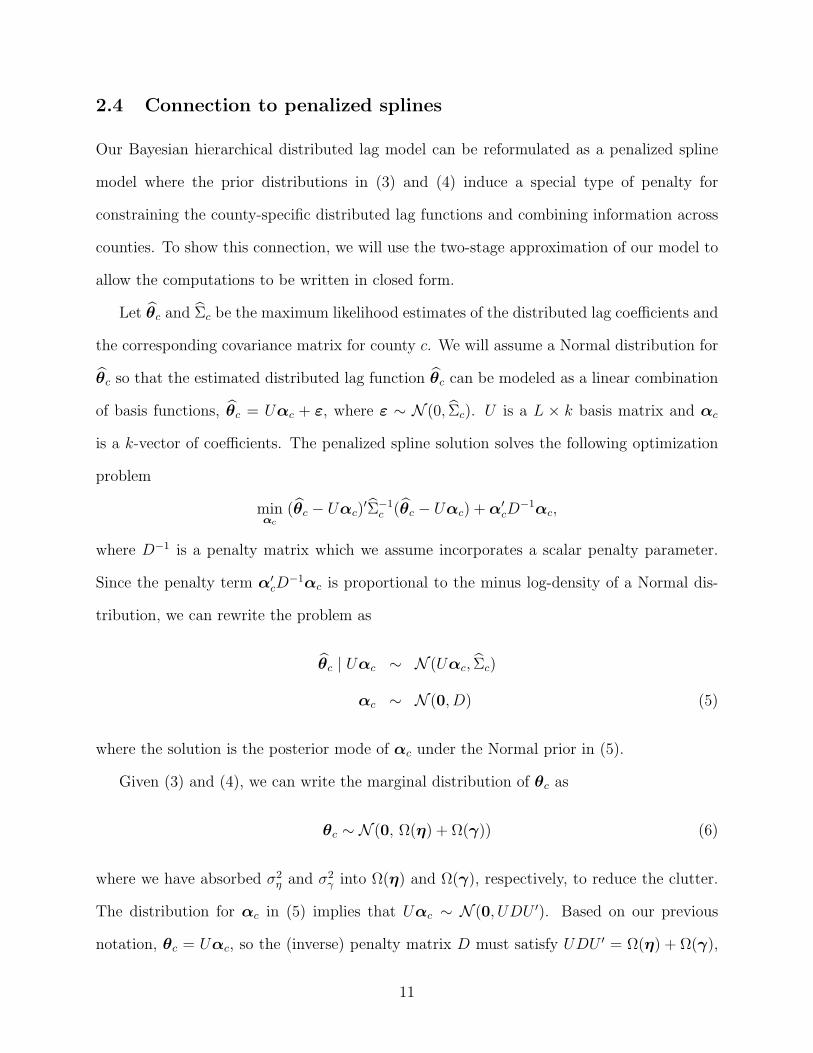
2.4 Connection to penalized splines
Our Bayesian hierarchical distributed lag model can be reformulated as a penalized spline
model where the prior distributions in (3) and (4) induce a special type of penalty for
constraining the county-specific distributed lag functions and combining information across
counties. To show this connection, we will use the two-stage approximation of our model to
allow the computations to be written in closed form.
Let θc and Σc be the maximum likelihood estimates of the distributed lag coefficients and
the corresponding covariance matrix for county c. We will assume a Normal distribution for
θc so that the estimated distributed lag function θc can be modeled as a linear combination
of basis functions, θc = Uαc + ε, where ε ∼ N (0, Σc). U is a L × k basis matrix and αc
is a k-vector of coefficients. The penalized spline solution solves the following optimization
problem
minαc
(θc − Uαc)′Σ−1
c (θc − Uαc) + α′cD
−1αc,
where D−1 is a penalty matrix which we assume incorporates a scalar penalty parameter.
Since the penalty term α′cD
−1αc is proportional to the minus log-density of a Normal dis-
tribution, we can rewrite the problem as
θc | Uαc ∼ N (Uαc, Σc)
αc ∼ N (0, D) (5)
where the solution is the posterior mode of αc under the Normal prior in (5).
Given (3) and (4), we can write the marginal distribution of θc as
θc ∼ N (0, Ω(η) + Ω(γ)) (6)
where we have absorbed σ2η and σ2
γ into Ω(η) and Ω(γ), respectively, to reduce the clutter.
The distribution for αc in (5) implies that Uαc ∼ N (0, UDU ′). Based on our previous
notation, θc = Uαc, so the (inverse) penalty matrix D must satisfy UDU ′ = Ω(η) + Ω(γ),
11

which has the solution
Dη,γ = (U ′U)−1U ′(Ω(η) + Ω(γ))U(U ′U)−1. (7)
Now we have shown that our prior distribution on θc can be translated into a penalty matrix
for spline coefficients αc in a penalized spline problem. Given values of η and γ and using
the penalty matrix in (7), we can calculate the penalized spline coefficient estimates as
αc = Dη,γU′(UDη,γU
′ + Σc)−1 θc and the smoothed county-specific distributed lag function
for county c is Uαc.
Similar calculations demonstrate how penalized splines can be used to combine the
county-specific distributed lag functions θc across counties. Analogous to (5), we can write
the the second level of our hierarchical model as
θc | Wδ ∼ N (Wδ, Ω(η)) [c = 1, . . . , n]
δ ∼ N (0, H) (8)
where W is a spline basis matrix, δ is a vector of coefficients, and H is a penalty matrix in
the penalized spline problem. The distribution in (4) and the prior for δ in (8) imply that
we need to find a matrix H such that WHW ′ = Ω(γ). The solution for H has the form
Hγ = (W ′W )−1W ′Ω(γ)W (W ′W )−1 and we can subsequently solve for δ = HγW′(WHγW
′+
Ω(η))−1 θ, where θ = (1/n)∑n
c=1 θc.
One can see that if we replace the basis matrices U and W with the L × L identity
matrix, then we revert back to our original formulation and obtain the same answers as our
original Bayesian hierarchical model. Our model places a prior directly on the distributed
lag function, while the penalized spline approach places a prior on the corresponding spline
coefficients. In this application it seems more natural to assume a prior distribution for the
distributed lag function directly because prior information is available in that domain.
12

3 Data
We apply our methods to national databases of hospitalization and ambient PM2.5 measure-
ments. The hospitalization data consist of daily counts of hospital admissions for the years
1999–2002 constructed from the National Claims History Files (NCHF) of the US Medicare
system, which contain the billing claims of all Medicare enrollees. Medicare enrollees make
up almost the entire US population over 65 years of age, or approximately 48 million people.
Each billing claim obtained from the NCHF contains the date of service, treatment, disease
classification (via International Classification of Diseases, Ninth Revision [ICD-9] codes),
age, gender, self-reported race, and place of residence (five digit ZIP code and county). The
daily counts for a given county were computed by summing the total number of hospitaliza-
tions with a primary diagnosis for a specific disease. For computing hospitalization rates, a
corresponding time series of the numbers of individuals at risk in each county for each day
was constructed.
The PM2.5 data were obtained from the US Environmental Protection Agency’s Air
Quality System database (formerly the AIRS database) which makes available data from a
national network of monitors. Before 1999, the EPA collected data on particulate matter
less than 10 µm in diameter (PM10), generally on a 1-in-6 day basis (i.e. for every six days,
one measurement of PM10 is made). Such a data collection pattern ruled out the use of
distributed lag models, which require data to be collected on consecutive days (although
daily PM10 data were collected for about 15 counties). Beginning in 1999, the EPA began
collecting PM2.5 data, generally on a 1-in-3 day basis, although there are over 100 counties
where measurements are taken everyday. With the emergence of the new PM2.5 monitoring
network, we can fit distributed lag models to data from more counties than previously
possible. Some counties contained more than one PM2.5 monitor, in which case we took a
10% trimmed mean of the daily values across monitors. In cases where there were less than
10 monitor readings, we dropped the lowest and highest values and averaged the remainder.
13

Finally, temperature and dew point temperature data were assembled from the National
Climatic Data Center on the Earth-Info CD database and linked by county with the pollution
and hospitalization data.
This analysis was necessarily restricted to the counties for which daily data on PM2.5 were
available. The included counties were further constrained to have a population over 200,000
and PM2.5 data spanning at least one full year. The resulting study population resided in
94 counties and consisted of of 6.3 million Medicare enrollees living on average 6 miles from
a PM2.5 monitor. The locations and populations of the 94 counties are shown in Figure 1.
For all of the counties used in this analysis, there were occasional missing PM2.5 values.
With the exception of the year 1999, when monitors in some counties were just beginning to
come into service, the missingness tended to be sporadic and seemingly at random. Rather
than treat the missing PM2.5 values specially or implement an imputation scheme, we chose
to simply drop missing observations and analyze only the days for which observations were
available. One issue that arises by taking this approach is that when fitting a distributed
lag model of order L, a single missing value in the exposure series propagates to create L
missing observations in the health effects model. Fortunately, the number of missing PM2.5
values was small enough so that this propagation did not cause a serious problem. There
were few, if any, missing values in the hospitalization and meteorological data.
4 Results
We applied the Bayesian hierarchical distributed lag model (BHDLM) to the 94 counties
with Medicare, air pollution, and weather data described in Section 3. The data for each
county spanned T = 1, 461 days (the 4 years from 1999 to 2002) and we chose to examine
two specific causes of hospitalization: chronic obstructive pulmonary disease with acute
exacerbation (COPDAE) and ischemic heart disease. These outcomes were chosen because
they represent common respiratory and cardiovascular diseases and have been shown in
14

previous studies to be strongly associated with PM2.5 exposure. Figure 2 shows boxplots
of the daily hospitalization rates for COPDAE and ischemic heart disease in each of the 94
counties. Figure 3 shows corresponding boxplots of the daily (log) PM2.5 data.
For the distributed lag function, we chose to fit a model with a maximum lag of two weeks,
so that L = 14 in (1). Since we were primarily interested in examining the short-term effects
of PM2.5, care had to be taken to ensure that L was not so large that longer-term effects
were implicitly included in the model. For comparison we also applied the step function
distributed lag model (Step DLM) described in Section 2.3 where the model is fit using the
two-stage approach.
The national average distributed lag functions estimated by the BHDLM for COPDAE
and ischemic heart disease are shown in Figure 4. Each of these plots shows the posterior
mean for µ plotted as a function of lag for each outcome as well as pointwise 95% posterior
intervals for each lag coefficient. At each lag the plotted coefficient can be interpreted as the
percent increase in hospitalization for a 10 µg/m3 increase in PM2.5. For COPDAE, Figure 4
suggests that PM2.5 is associated with two “waves” of admissions, with the first arriving 1
day after the increase and the second arriving a few days later. For ischemic heart disease,
there is about a 0.24% increase in admissions on the same day, followed by an approximately
0.35% decrease in admissions on the following day. At lag 2, the relative risk jumps to a
0.6% increase in admissions, beyond which the distributed lag function for ischemic heart
disease is essentially zero.
The joint marginal posterior distributions for γ1 and γ2, which control the tapering and
smoothness of µ, are shown in Figure 5 for both COPDAE and ischemic heart disease. Large
values of γ1 indicate a strong tapering of the lag coefficients towards zero while large values
of γ2 indicate a very smooth distributed lag function. The data for both outcomes prefer
a large value for γ1, indicating strong variance tapering, but for ischemic heart disease the
marginal distribution for γ2 is shifted somewhat higher than that of COPDAE.
15

The county-specific Bayesian distributed lag functions for COPDAE and ischemic heart
disease are are shown in Figures 6 and 7, respectively. Each figure shows the posterior
mean and pointwise 95% posterior intervals of θc for the largest 25 counties in the study.
For COPDAE, the estimated county-specific distributed lag functions are a mix of shapes
including large immediate effects (Sacramento CA, Broward FL), somewhat smaller delayed
effects (Los Angeles CA, Franklin OH, Pinellas FL), and more moderate effects spread out
over a longer period of time (Bronx NY, Palm Beach FL, Salt Lake UT). Ischemic heart
disease appears to exhibit somewhat less heterogeneity in the shapes of the distributed lag
functions with most of the effects occurring at lags 0–2. In Fairfax VA and Pinellas FL
counties appears to be some evidence of mortality displacement.
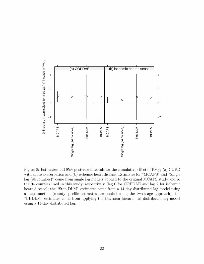
Figure 8 shows the posterior mean and 95% posterior intervals of the cumulative effect of
PM2.5 on both outcomes from four different models. For each outcome we plot the estimate
originally reported in the MCAPS study for a single lag model applied to 204 US coun-
ties (Dominici et al., 2006), the estimate obtained from a single lag model applied to the 94
counties used in this study (for the exposure lag we chose lag 0 for COPDAE and lag 2 for
ischemic heart disease, the same lags used in MCAPS), the estimate obtained from using the
two-stage approach, and the estimate obtained from our Bayesian hierarchical distributed
lag model (BHDLM).
The estimates of the cumulative effects for COPDAE and ischemic heart disease are
remarkably similar across models. The MCAPS point estimate was reported as 0.91 with
a 95% posterior interval of (0.18, 1.64) and posterior mean from the BHDLM model was
0.84 (−2.06, 3.78). One can see from the difference in posterior intervals from the “MCAPS”
and the “Single lag” estimates that the loss of 110 counties in this study only results in
a small loss of efficiency in the estimate of the single lag effect. In the distributed lag
model, the increased number of parameters introduced (even in the 3-parameter “Step DLM”
model) results in a substantial increase in the variance of the cumulative effect estimate. For
16

the ischemic heart disease outcome, the estimate from the BHDLM is 0.66 (−1.55, 2.89)
compared to the MCAPS estimate of 0.44 (0.02, 0.86). This higher effect was also captured
by the step-function distributed lag model but the estimate from the BHDLM appears to
exhibit less variance in its estimate.
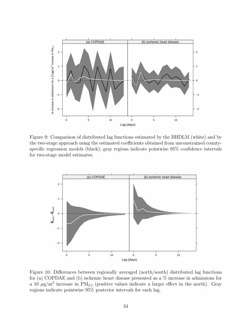
One concern raised by applying our Bayesian distributed lag model is the possibility that
placing constraints on the parameters corresponding to longer lags would somehow introduce
bias in estimates of parameters corresponding to shorter lags. To investigate this concern
we estimated the national average distributed lag function using both our BHDLM and a
completely unconstrained two-stage model and plotted both estimates in Figure 9. One can
see that for ischemic heart disease, the estimates at lags 0–3 for both models are very similar,
after which the BHDLM estimates are all close to zero. For COPDAE the estimates for lags
0–2 are relatively close; after lag 3 the BHDLM estimates become much more smooth than
the unconstrained estimates. For both outcomes it appears that imposing constraints on the
longer lags does not substantially bias the estimates at shorter lags in the sense that estimates
at shorter lags are similar to those that would have been obtained using an unconstrained
model.
4.1 Regional variation
One significant advantage of our analysis is that it provides the opportunity to examine
variation in the county-specific distributed lag functions across locations and regions. In
particular, regional variation in the composition of PM2.5 may correspond with variation in
the estimated distributed lag functions if the concentrations of most toxic constituents of
the PM mixture vary across locations (Bell et al., 2007; Lippmann et al., 2006). Variation
in the estimated relative risks may also indicate regional variation in the susceptibilities in
the underlying populations to exposure to PM2.5.
We compared the estimated county-specific distributed lag functions for 53 counties in
17

the Northern region of the US (defined as having latitude > 36.5) with 41 counties in the
Southern region of the US to see if there were any systematic differences. Given the N
posterior samples of the county-specific distributed lag functions θc, we calculated regional
averages
θ(i)R =
1
nR
∑c∈IR
θ(i)c
for each of the posterior samples i, where R indicates the region (North or South) and IR
is the index set for the counties in region R. The posterior mean θR was then computed by
averaging θ(i)R over the posterior samples.
Figure 10 shows θnorth−θsouth, the difference between the Northern and Southern regional
average distributed lag functions. The negative differences in Figure 10(a) indicate a stronger
association between PM2.5 and COPDAE in the South than in the North. These differences
appear to extend to approximately a 3–4 day lag after which the difference quickly disappears.
For the ischemic heart disease outcome the reverse appears to be true, with Figure 10(b)
indicating that counties in the North experience a stronger association between PM2.5 and
admissions for ischemic heart disease.
Examination of the cumulative effects for the North and South show a clear regional
difference. For each posterior sample we calculated ξ(i)R =
∑L−1`=0 θ
(i)R,` and plotted the joint
posterior distribution of the North and South cumulative effects in Figure 11. For COPDAE,
the bulk of the posterior mass is above the dashed line indicating the relation y = x, providing
evidence of a larger cumulative effect of PM2.5 in the South, with a posterior probability
P(ξsouth > ξnorth | data) = 0.93. For ischemic heart disease, the posterior mass is concentrated
below the line y = x, indicating a larger effect in the North with P(ξnorth > ξsouth | data) =
0.95.
As shown in Figure 1, the majority of the Northern and Southern counties are in the
eastern portion of the country and hence the North/South comparison is largely a comparison
of counties in the northeast and industrial midwest with counties in the southeast and south-
18
central regions. The major constituents of PM pollution in the northeastern region include
sulfate and ammonium, which originate largely from power generation sources, while PM
in the southeastern region generally contains more silicon, an element related to crustal
material and mechanical processes (Bell et al., 2007). Also, the change in latitude from the
North to the South covers a wide range of temperatures and climates which may alter the
susceptibilities of populations to air pollution exposure.
5 Discussion
We have proposed a Bayesian hierarchical distributed lag model (BHDLM) for combining
constrained distributed lag functions and for estimating the distributed lag between day-to-
day changes in ambient air pollution levels and day-to-day changes in hospitalization rates.
The model uses a prior distribution that constrains the time course of the short-term health
effects of air pollution and combines information from multiple locations. We have applied
the model to a national air pollution and hospitalization database for United States residents
enrolled in Medicare, examining the relationship between PM2.5 exposure and hospitalization
for ischemic heart disease and COPD with acute exacerbation.
The model that we have proposed allows us to summarize information contained in
national databases and quantify how the risk of hospitalization due to air pollution exposure
changes over short periods of time after an air pollution episode. Our model builds on
the work of Welty et al. (2005) and Zanobetti et al. (2000) by smoothing distributed lag
function estimates across lags and by providing a method for combining these functions across
locations where we assume more variability for parameters corresponding to shorter lags and
less variability for parameters corresponding to longer lags. In addition, the hierarchical
model lets us examine the range of shapes in the county-specific distributed lag functions, as
shown in Figures 6 and 7. We have established that our methodology is related to penalized
spline modeling with a special type of penalty and this connection, along with evidence from
19

simulation studies conducted by Welty et al. (2005), creates a basis for understanding the
statistical properties of our approach.
The national average distributed lag functions for COPDAE and ischemic heart disease
indicate different time courses for the effect of PM2.5 on hospitalizations for these disease cat-
egories. The effect of PM2.5 on COPDAE admissions appears to be spread over a longer time
period than the effect on ischemic heart disease admissions. The nature and characteristics
of acute exacerbations of COPD are known to be heterogeneous across people (Sapey and
Stockley, 2006) and exacerbations are often a cause of hospitalization after initial treatment
outside the hospital has failed (Seemungal et al., 2000). We found little evidence that the
effect of an increase in PM2.5 levels on hospitalizations for ischemic heart disease extends
beyond 2 days. In addition, the shape of the distributed lag function for ischemic heart dis-
ease suggests some weak evidence of mortality displacement. Cardiovascular effects of PM
are thought to be generally related to neurogenic and inflammatory processes (Pope et al.,
2003). The results from our analysis suggest that for ischemic heart disease in particular,
the biological mechanism involved has a relatively short time course, with the bulk of people
admitted to the hospital within two days of an increase in PM2.5 levels.
When estimating the cumulative effect of PM2.5 on either health outcome, there ap-
pears to be a bias-variance trade off involved in choosing between applying a single lag or
distributed lag model. Even with the national databases used here, estimation of the dis-
tributed lag function resulted in a substantial increase in the variance of the cumulative
effect compared to risk estimates from single lag models. While one might consider the sin-
gle lag model’s restriction to fixed lag effects a limitation (and potentially a source of bias),
one must also consider the dramatic increase in precision that the model provides. If the
cumulative short-term effect of an increase in air pollution levels is the sole parameter of
interest, the benefits of the distributed lag model’s greater flexibility may not outweigh the
cost of incurring much greater variability in the resulting estimate.
20

We should be careful not to overinterpret the findings of our analysis. Even with the
constraints imposed by the prior, the uncertainty of the estimates in Figure 4 is still large,
particularly for coefficients corresponding to early lags. In addition, Medicare data are
collected for administrative purposes and disease diagnoses are known to be subject to some
missclassification. However, such missclassification would only bias our results if the daily
pattern of diagnosis and coding varied in a way that was correlated with PM2.5 levels.
One limitation of our application of the BHDLM is the reliance on the Poisson distribution
in the county-specific model in (2). While previous time series studies of air pollution and
health have suggested that there is relatively little overdispersion in the residuals, a more
flexible alternative might be to use a generalized Poisson model as in Fuentes et al. (2006).
Another point of discussion concerns the prior distributions used in this application. We
have placed uniform hyperprior distributions on η and γ which place equal prior weight
on models which may not be equally plausible. Nevertheless, the posterior distributions in
Figure 5 suggest that there is some information in the data to choose between these models.
Also, the specific use of an exponential decay in the variance of the lag coefficients does affect
the resulting shape of the estimated distributed lag function somewhat. We have explored
alternative decay functions such as a half-Normal and power law and our analyses indicate
that these alternatives do not affect the substantive conclusions of the investigation.
Our model did not include any interactions between levels of PM2.5 on different days
or with averages of PM2.5 levels over several days. It is plausible that such interactions
exist and if so, estimates from our model would likely be biased. In our initial exploratory
analyses models containing simple interactions were fit and we generally found little evidence
to support their inclusion. Nevertheless, the development of a more structured approach to
the estimation of interactions as well as the development of appropriate prior distributions
is an important direction for future work.
The principal benefit of the distributed lag model is its ability to estimate the shape of
21
the distributed lag function relating increases in air pollution to health outcomes in short
periods of time after an air pollution episode. Our model provides a useful parametrization
that can easily incorporate prior knowledge and be applied to large multi-site databases.
Over time, as more data become available from national databases, our model could be
applied to track the health effects of particulate matter. While the results of our analysis are
interesting and suggest some possible hypotheses, more focused studies (perhaps involving
compositional data on PM2.5 or susceptible sub-populations) will have to be conducted to
obtain more precise information about the biological mechanisms involved.
Acknowledgements
This research was supported in part by a Faculty Innovation Fund award from the Johns
Hopkins Bloomberg School of Public Health, grant RD-83241701 from the US Environmental
Protection Agency, the NIEHS Center in Urban Environmental Health (grant P30ES03819),
and grant ES012054-03 from the National Institute of Environmental Health Sciences.
References
Almon, S. (1965), “The distributed lag between capital appropriations and expenditures,”
Econometrica, 33, 178–196.
Bell, M. L., Dominici, F., Ebisu, K., Zeger, S. L., and Samet, J. M. (2007), “Spatial and
temporal variation in PM2.5 chemical composition in the United States for health effects
studies,” Environmental Health Perspectives, 115, 989–995.
Bell, M. L., McDermott, A., Zeger, S. L., Samet, J. M., and Dominici, F. (2004), “Ozone and
Short-term Mortality in 95 US Urban Communities, 1987-2000,” Journal of the American
Medical Association, 292, 2372–2378.
22

Chatfield, C. (1996), The Analysis of Times Series: An Introduction, Chapman & Hall/CRC,
5th ed.
Corradi, C. (1977), “Smooth distributed lag estimators and smoothing spline functions in
Hilbert spaces,” Journal of Econometrics, 5, 211–220.
Dominici, F., Daniels, M., Zeger, S. L., and Samet, J. M. (2002a), “Air Pollution and
Mortality: Estimating Regional and National Dose-Response Relationships,” Journal of
the American Statistical Association, 97, 100–111.
Dominici, F., McDermott, A., Zeger, S. L., and Samet, J. M. (2002b), “Airborne partic-
ulate matter and mortality: Time-scale effects in four US Cities,” American Journal of
Epidemiology, 157, 1053–1063.
Dominici, F., Peng, R. D., Bell, M. L., Pham, L., McDermott, A., Zeger, S. L., and Samet,
J. M. (2006), “Fine Particulate Air Pollution and Hospital Admission for Cardiovascular
and Respiratory Diseases,” Journal of the American Medical Association, 295, 1127–1134.
Everson, P. J. and Morris, C. N. (2000), “Inference for Multivariate Normal Hierarchical
Models,” Journal of the Royal Statistical Society, Series B, 62, 399–412.
Fuentes, M., Song, H.-R., Ghosh, S. K., Holland, D. M., and Davis, J. M. (2006), “Spatial
Association between Speciated Fine Particles and Mortality,” Biometrics, 62, 855–863.
Goodman, P. G., Dockery, D. W., and Clancy, L. (2004), “Cause-specific mortality and
the extended effects of particulate pollution and temperature exposure,” Environmental
Health Perspectives, 112, 179–185.
Health Effects Institute (2003), Revised Analyses of Time-Series Studies of Air Pollution
and Health. Special Report., Health Effects Institute, Boston MA.
23
Huang, Y., Dominici, F., and Bell, M. L. (2005), “Bayesian Hierarchical Distributed Lag
Models for Summer Ozone Exposure and Cardio-Respiratory Mortality,” Environmetrics,
16, 547–562.
Jones, G. L., Haran, M., Caffo, B. S., and Neath, R. (2006), “Fixed-Width Output Analysis
for Markov Chain Monte Carlo,” Journal of the American Statistical Association, 101,
1537–1547.
Katsouyanni, K., Toulomi, G., Samoli, E., Gryparis, A., LeTertre, A., Monopolis, Y., Rossi,
G., Zmirou, D., Ballester, F., Boumghar, A., and Anderson, H. R. (2001), “Confounding
and Effect Modification in the Short-term Effects of Ambient Particles on Total Mortality:
Results from 29 European Cities within the APHEA2 Project,” Epidemiology, 12, 521–531.
Kelsall, J. E., Samet, J. M., Zeger, S. L., and Xu, J. (1997), “Air Pollution and Mortality in
Philadelphia, 1974–1988,” American Journal of Epidemiology, 146, 750–762.
Leamer, E. E. (1972), “A class of informative priors and distributed lag analysis,” Econo-
metrica, 40, 1059–1081.
Lippmann, M., Ito, K., Hwang, J.-S., Maciejczyk, P., and Chen, L.-C. (2006), “Cardiovascu-
lar Effects of Nickel in Ambient Air,” Environmental Health Perspectives, 114, 1662–1669.
Peng, R. D., Dominici, F., and Louis, T. A. (2006), “Model choice in time series studies
of air pollution and mortality (with discussion),” Journal of the Royal Statistical Society,
Series A, 169, 179–203.
Peng, R. D., Dominici, F., Pastor-Barriuso, R., Zeger, S. L., and Samet, J. M. (2005),
“Seasonal Analyses of Air Pollution and Mortality in 100 US Cities,” American Journal
of Epidemiology, 161, 585–594.
Pope, C. A., Burnett, R. T., Thruston, G. D., Calle, E., Thun, M. J., Krewski, D., and
Goldeski, J. (2003), “Cardiovascular Mortality and Long-term Exposure to Particulate Air
24

Pollution: Epidemiological Evidence of General Pathophysiological Pathways of Disease,”
Circulation, 6, 71–77.
Pope, C. A. and Dockery, D. W. (2006), “Health effects of fine particulate air pollution: lines
that connect,” Journal of the Air and Waste Management Association, 56, 709–742.
R Development Core Team (2006), R: A Language and Environment for Statistical Comput-
ing, R Foundation for Statistical Computing, Vienna, Austria, ISBN 3-900051-07-0.
Roberts, S. (2005), “An investigation of distributed lag models in the context of air pol-
lution and mortality time series analysis,” Journal of the Air and Waste Management
Association, 55, 273–282.
Samoli, E., Touloumi, G., Zanobetti, A., Le Tertre, A., Schindler, C., Atkinson, R., Vonk,
J., Rossi, G., Saez, M., Rabczenko, D., Schwartz, J., and Katsouyanni, K. (2003), “In-
vestigating the dose-response relation between air pollution and total mortality in the
APHEA-2 multicity project,” Occupational and Environmental Medicine, 60, 977–982.
Sapey, E. and Stockley, R. A. (2006), “COPD exacerbations 2: Aetiology,” Thorax, 61,
250–258.
Schimmel, H. and Murawski, T. J. (1976), “The relation of air pollution to mortality,”
Journal of Occupational Medicine, 18, 316–333.
Schmidt, A. M., de Fatima da G. Conceicao, M., and Morerira, G. A. (2007), “Investigating
the sensitivity of Gaussian processes to the choice of their correlation function and prior
specifications,” Journal of Statistical Computation and Simulation, to appear.
Schwartz, J. (2000), “The Distributed Lag between Air Pollution and Daily Deaths,” Epi-
demiology, 11, 320–326.
25

Seemungal, T. A. R., Donaldson, G. C., Bhowmik, A., Jeffries, D. J., and Wedzicha, J. A.
(2000), “Time Course and Recovery of Exacerbations in Patients with Chronic Obstructive
Pulmonary Disease,” American Journal of Respiratory and Critical Care Medicine, 161,
1608–1613.
Shiller, R. J. (1973), “A distributed lag estimator derived from smoothness priors,” Econo-
metrica, 41, 775–788.
Welty, L. J. and Zeger, S. L. (2005), “Are the Acute Effects of PM10 on Mortality in
NMMAPS the Result of Inadequate Control for Weather and Season? A Sensitivity Anal-
ysis using Flexible Distributed Lag Models.” American Journal of Epidemiology, 162,
80–88.
Welty, L. J., Zeger, S. L., and Dominici, F. (2005), “Bayesian Distributed Lag
Models: Estimating the Effects of Particulate Matter Air Pollution on Daily
Mortality,” Tech. Rep. 96, Johns Hopkins University Department of Biostatistics,
http://www.bepress.com/jhubiostat/paper96.
Zanobetti, A., Schwartz, J., Samoli, E., Gryparis, A., Touloumi, G., Atkinson, R., Le Tertre,
A., Bobros, J., Celko, M., Goren, A., Forsberg, B., Michelozzi, P., Rabczenko, D.,
Aranguez, R. E., and Katsouyanni, K. (2002), “The temporal pattern of mortality re-
sponses to air pollution: a multicity assessment of mortality displacement,” Epidemiology,
13, 87–93.
Zanobetti, A., Wand, M., Schwartz, J., and Ryan, L. (2000), “Generalized additive dis-
tributed lag models: quantifying mortality displacement,” Biostatistics, 1, 279–292.
Zeger, S. L., Dominici, F., and Samet, J. M. (1999), “Harvesting-resistant estimates of
pollution effects on mortality,” Epidemiology, 89, 171–175.
26

A Figures
0.1 0.3 0.4 0.5 0.7 0.8 0.9 1.4 9.5
Population (in millions)
Figure 1: Locations of 94 U.S. counties which have daily data for particulate matter < 2.5 µmin diameter for 1999–2002.
27

Daily hospitalization rate per 10,000
0 1 2 3 4 5 6
Adams, PAAllegan, MIMercer, PA
Scott, IAJackson, OR
Clay, MORichmond, VA
Chesapeake, VALackawanna, PA
Durham, NCTrumbull, OHDauphin, PA
Jefferson, TXSpartanburg, SC
Mahoning, OHNorthampton, PA
Forsyth, NCCharleston, SC
Lane, ORButler, OH
St. Louis, MOPulaski, AR
Polk, IAGreenville, SC
Knox, TNE. Baton Rouge, LA
Spokane, WAGuilford, NC
Lucas, OHJefferson, LA
Hampden, MAOrleans, LA
New Castle, DERamsey, MN
Union, NJSummit, OHDenver, CO
Bernalillo, NMMontgomery, OH
Tulsa, OKDavidson, TN
Washington, DCKent, MI
Wake, NCBaltimore, MDJackson, MO
Oklahoma, OKMultnomah, OR
Kern, CAJefferson, AL
DeKalb, GAEl Paso, TXSuffolk, MA
Jefferson, KYMecklenburg, NC
Pierce, WAWorcester, MA
Duval, FLFresno, CA
Travis, TXFulton, GA
New Haven, CTPima, AZ
Hamilton, OHHartford, CT
Marion, INHonolulu, HIOrange, FLShelby, TN
Salt Lake, UTPinellas, FL
Milwaukee, WIFairfax, VA
Hillsborough, FLFranklin, OH
Hennepin, MNPalm Beach, FLSacramento, CA
Allegheny, PABronx, NYClark, NVBexar, TX
Cuyahoga, OHBroward, FL
King, WAWayne, MIDallas, TX
Miami−Dade, FLSan Diego, CA
Maricopa, AZHarris, TX
Cook, ILLos Angeles, CA
0 1 2 3 4 5 6
COPDAE
0 1 2 3 4 5 6
0 1 2 3 4 5 6
ischemic heart disease
Figure 2: Boxplots of daily hospitalization rates (per 10,000 people) for COPDAE andischemic heart disease for 94 U.S. counties, 1999–2002.
28

log10((PM2.5)) level in µµg m3
−1 0 1 2
Adams, PAAllegan, MIMercer, PA
Scott, IAJackson, OR
Clay, MORichmond, VA
Chesapeake, VALackawanna, PA
Durham, NCTrumbull, OHDauphin, PA
Jefferson, TXSpartanburg, SC
Mahoning, OHNorthampton, PA
Forsyth, NCCharleston, SC
Lane, ORButler, OH
St. Louis, MOPulaski, AR
Polk, IAGreenville, SC
Knox, TNE. Baton Rouge, LA
Spokane, WAGuilford, NC
Lucas, OHJefferson, LA
Hampden, MAOrleans, LA
New Castle, DERamsey, MN
Union, NJSummit, OHDenver, CO
Bernalillo, NMMontgomery, OH
Tulsa, OKDavidson, TN
Washington, DCKent, MI
Wake, NCBaltimore, MDJackson, MO
Oklahoma, OKMultnomah, OR
Kern, CAJefferson, AL
DeKalb, GAEl Paso, TXSuffolk, MA
Jefferson, KYMecklenburg, NC
Pierce, WAWorcester, MA
Duval, FLFresno, CA
Travis, TXFulton, GA
New Haven, CTPima, AZ
Hamilton, OHHartford, CT
Marion, INHonolulu, HIOrange, FLShelby, TN
Salt Lake, UTPinellas, FL
Milwaukee, WIFairfax, VA
Hillsborough, FLFranklin, OH
Hennepin, MNPalm Beach, FLSacramento, CA
Allegheny, PABronx, NYClark, NVBexar, TX
Cuyahoga, OHBroward, FL
King, WAWayne, MIDallas, TX
Miami−Dade, FLSan Diego, CA
Maricopa, AZHarris, TX
Cook, ILLos Angeles, CA
−1 0 1 2
Figure 3: Boxplots of the daily log10 PM2.5 values for 94 U.S. counties, 1999–2002.
29

Lag (days)
% in
crea
se in
adm
issi
ons
for
a 10
µµg
m3 in
crea
se in
PM
2.5
−1
0
1
0 5 10
(a) COPDAE
0 5 10
(b) ischemic heart disease
Figure 4: National average distributed lag functions for (a) COPD with acute exacerbationand (b) ischemic heart disease from the Bayesian hierarchical distributed lag model applied to94 U.S. counties, 1999–2002. Each plot shows the posterior mean (white line) and pointwise95% posterior intervals (shaded gray region) for each lag coefficient.
γγ1
γγ 2
0.2
0.4
0.6
0.2 0.4 0.6
COPDAE
0.2 0.4 0.6
ischemic heart disease
0.0
0.5
1.0
1.5
2.0
2.5
3.0
3.5
Figure 5: Joint marginal posterior distributions for γ1 and γ2 for both COPDAE and ischemicheart disease.
30

Lag (days)
% in
crea
se in
adm
issi
ons
for
a 10
µµg
m3 in
crea
se in
PM
2.5
−5
0
5
Los Angeles, CA
0 5 10
Cook, IL Harris, TX
0 5 10
Maricopa, AZ San Diego, CA
Miami−Dade, FL Dallas, TX Wayne, MI King, WA
−5
0
5
Broward, FL
−5
0
5
Cuyahoga, OH Bexar, TX Clark, NV Bronx, NY Allegheny, PA
Sacramento, CA Palm Beach, FL Hennepin, MN Franklin, OH
−5
0
5
Hillsborough, FL
−5
0
5
0 5 10
Fairfax, VA Milwaukee, WI
0 5 10
Pinellas, FL Salt Lake, UT
0 5 10
Shelby, TN
Figure 6: County-specific Bayesian distributed lag functions (with pointwise 95% posteriorintervals) showing the effect of PM2.5 on hospitalization for COPD with acute exacerbation.Only the largest 25 counties (by population) are shown here, with the largest county (LosAngeles, CA) in the top left corner.
31

Lag (days)
% in
crea
se in
adm
issi
ons
for
a 10
µµg
m3 in
crea
se in
PM
2.5
−5
0
5
Los Angeles, CA
0 5 10
Cook, IL Harris, TX
0 5 10
Maricopa, AZ San Diego, CA
Miami−Dade, FL Dallas, TX Wayne, MI King, WA
−5
0
5
Broward, FL
−5
0
5
Cuyahoga, OH Bexar, TX Clark, NV Bronx, NY Allegheny, PA
Sacramento, CA Palm Beach, FL Hennepin, MN Franklin, OH
−5
0
5
Hillsborough, FL
−5
0
5
0 5 10
Fairfax, VA Milwaukee, WI
0 5 10
Pinellas, FL Salt Lake, UT
0 5 10
Shelby, TN
Figure 7: County-specific Bayesian distributed lag functions (with pointwise 95% posteriorintervals) showing the effect of PM2.5 on hospitalization for ischemic heart disease. Only thelargest 25 counties (by population) are shown here, with the largest county (Los Angeles,CA) in the top left corner.
32
% in
crea
se in
adm
issi
ons
for
a 10
µµg
m3 in
ceas
e in
PM
2.5
−2
0
2
4
MC
AP
S
Sin
gle
lag
(94
coun
ties)
Ste
p D
LM
BH
DLM
(a) COPDAE
MC
AP
S
Sin
gle
lag
(94
coun
ties)
Ste
p D
LM
BH
DLM
−2
0
2
4
(b) ischemic heart disease
Figure 8: Estimates and 95% posterior intervals for the cumulative effect of PM2.5 (a) COPDwith acute exacerbation and (b) ischemic heart disease. Estimates for “MCAPS” and “Singlelag (94 counties)” come from single lag models applied to the original MCAPS study and tothe 94 counties used in this study, respectively (lag 0 for COPDAE and lag 2 for ischemicheart disease); the “Step DLM” estimates come from a 14-day distributed lag model usinga step function (county-specific estimates are pooled using the two-stage approach); the“BHDLM” estimates come from applying the Bayesian hierarchical distributed lag modelusing a 14-day distributed lag.
33
Lag (days)
% in
crea
se in
adm
issi
ons
for
a 10
µµg
m3 in
ceas
e in
PM
2.5
−2
−1
0
1
2
0 5 10
(a) COPDAE
0 5 10
−2
−1
0
1
2
(b) ischemic heart disease
Figure 9: Comparison of distributed lag functions estimated by the BHDLM (white) and bythe two-stage approach using the estimated coefficients obtained from unconstrained county-specific regression models (black); gray regions indicate pointwise 95% confidence intervalsfor two-stage model estimates.
Lag (days)
θθ nor
th−−
θθ sou
th
−2
−1
0
1
2
0 5 10
(a) COPDAE
0 5 10
(b) ischemic heart disease
Figure 10: Differences between regionally averaged (north/south) distributed lag functionsfor (a) COPDAE and (b) ischemic heart disease presented as a % increase in admissions fora 10 µg/m3 increase in PM2.5 (positive values indicate a larger effect in the north). Grayregions indicate pointwise 95% posterior intervals for each lag.
34

−6 −4 −2 0 2 4
−4
−2
02
46
810
(a) COPDAE
Cumulative effect (North)
Cum
ulat
ive
effe
ct (
Sou
th)
−2 0 2 4 6
−4
−2
02
4
(a) ischemic heart disease
Cumulative effect (North)
Cum
ulat
ive
effe
ct (
Sou
th)
Figure 11: Joint posterior distributions of the cumulative effects for the North and Southregions for the (a) COPDAE and (b) ischemic heart disease outcomes; the dashed lineindicates the line y = x.
35

B Details of Gibbs Sampler
We implement a hybrid Gibbs sampler to sample from the posterior distributions of η, γ,
θc (c = 1, . . . , n), and µ. Briefly, the full conditionals for η, γ, and θc for c = 1, . . . , n are
sampled using a Metropolis-Hastings rejection step and the full conditional for µ is sampled
in closed form. All calculations were done using R version 2.4.1 (R Development Core Team,
2006). We describe the procedures for sampling from the full conditional distributions below.
1. Sampling θc. In order to sample from the full conditional for θc we implement a
Metropolis-Hastings rejection scheme. Sampling from the full conditional for θc re-
quires evaluting the likelihood for county c with both θc and the nuisance parameters
in βc. Rather than assume a prior distribution for the many nuisance parameters in
βc, we evaluate the profile likelihood Lp(θc) = maxβcLf (θc, βc), where for each given
value of θc, we maximize the full Poisson likelihood Lf with respect to βc, holding θc
fixed. In the Metropolis-Hastings step taken to sample from the full conditional for θc,
we use the profile likelihood for θc to calculate the acceptance ratio for the proposal.
The proposal distribution for sampling from the full conditional of θc is constructed
by first estimating θc in a county-specific log-linear Poisson regression model to obtain
θc and its estimated covariance matrix Σc. If we assume as in the two-stage approach
that θc | θc ∼ N (θc, Σc), we can compute the conditional distribution of θc given θc
and the current values of µ and γ and use this conditional distribution as a proposal
distribution, i.e.
θ∗c | θc, µ, γ ∼ N (µ + B1(θc − µ), σ2
γ(I −B1)Ω(γ)) (9)
where B1 = σ2γΩ(γ) [Σc + σ2
γΩ(γ)]−1. Given the proposal distribution in (9), the full
conditional for θc is then proportional to
p(θc | ·) ∝ Lp(θc)ϕ(θc | µ, σ2ηΩ(η))
36

where ϕ(θc | µ, σ2ηΩ(η)) is the multivariate normal density with mean µ and covariance
matrix σ2ηΩ(η) and Lp(θc) is the profile likelihood for θc.
2. Sampling µ. The full conditional for µ is proportional to
p(µ | ·) ∝
n∏
c=1
ϕ(θc | µ, σ2ηΩ(η))
ϕ(µ | 0, σ2
γΩ(γ))
= N (B2 θ, (I −B2) σ2γΩ(γ))
where B2 = σ2γΩ(γ) [σ2
γΩ(γ) + σ2ηΩ(η)/n]−1 and θ = 1
n
∑θc.
3. Sampling η and γ. We put uniform priors on both η = (η1, η2) and γ = (γ1, γ2) and
hence the full conditionals for η and γ are
p(η | ·) ∝n∏
c=1
ϕ(θc | µ, σ2ηΩ(η))
and
p(γ | ·) ∝ ϕ(µ | 0, σ2γΩ(γ)).
In order to preserve numerical stability, we placed upper and lower bounds on each
parameter so that both η1 and η2 were restricted to be in the range [0.2, 0.8] while
γ1 and γ2 were restricted to be in the range [0.05, 0.75]. These bounds were chosen
based on previous work and some exploratory analysis. Upper bounds that were much
larger than these values often produced covariance matrices that were not invertible.
We subsequently used uniform proposal distributions (restricted to the appropriate
ranges) and a Metropolis-Hastings rejection step to sample from the full conditionals
of η and γ.
The Gibbs samplers for each hospitalization outcome were each run for 40,000 iterations
with 10,000 iterations discarded as burn-in. Acceptance percentages for the Metropolis-
Hastings steps were tuned to be between 10–30%. Convergence of the chains was diagnosed
by estimating Monte Carlo standard errors of the parameters using the method of batch
means described in Jones et al. (2006).
37