job mismatches and labour market outcomes: panel ...ftp.iza.org/dp5083.pdfiza discussion paper no....
TRANSCRIPT

DI
SC
US
SI
ON
P
AP
ER
S
ER
IE
S
Forschungsinstitut zur Zukunft der ArbeitInstitute for the Study of Labor
Job Mismatches and Labour Market Outcomes:Panel Evidence on Australian University Graduates
IZA DP No. 5083
July 2010
Kostas MavromarasSeamus McGuinnessNigel O’Leary
Peter SloaneZhang Wei

Job Mismatches and Labour Market Outcomes: Panel Evidence on
Australian University Graduates
Kostas Mavromaras NILS, Flinders University and IZA
Seamus McGuinness
ESRI, Dublin
Nigel O’Leary WELMERC, Swansea University
Peter Sloane
WELMERC, Swansea University, NILS, Flinders University and IZA
Zhang Wei
NILS, Flinders University
Discussion Paper No. 5083 July 2010
IZA
P.O. Box 7240 53072 Bonn
Germany
Phone: +49-228-3894-0 Fax: +49-228-3894-180
E-mail: [email protected]
Any opinions expressed here are those of the author(s) and not those of IZA. Research published in this series may include views on policy, but the institute itself takes no institutional policy positions. The Institute for the Study of Labor (IZA) in Bonn is a local and virtual international research center and a place of communication between science, politics and business. IZA is an independent nonprofit organization supported by Deutsche Post Foundation. The center is associated with the University of Bonn and offers a stimulating research environment through its international network, workshops and conferences, data service, project support, research visits and doctoral program. IZA engages in (i) original and internationally competitive research in all fields of labor economics, (ii) development of policy concepts, and (iii) dissemination of research results and concepts to the interested public. IZA Discussion Papers often represent preliminary work and are circulated to encourage discussion. Citation of such a paper should account for its provisional character. A revised version may be available directly from the author.

IZA Discussion Paper No. 5083 July 2010
ABSTRACT
Job Mismatches and Labour Market Outcomes: Panel Evidence on Australian University Graduates*
The interpretation of graduate mismatch manifested either as overeducation or as overskilling remains problematical. This paper uses annual panel information on both educational and skills mismatches uniquely found in the HILDA survey to analyse the relationship of both mismatches with pay, job satisfaction and job mobility. We find that overeducation and overskilling are distinct phenomena with different labour market outcomes and that their combination results in the most severe negative labour market outcomes. Using panel methodology reduces strongly the size of many relevant coefficients, questioning previous cross-section results and suggesting the presence of considerable unobserved heterogeneity which varies by gender. JEL Classification: J24, J31 Keywords: overeducation, overskilling, wages, satisfaction, mobility Corresponding author: Kostas Mavromaras National Institute of Labour Studies Flinders University GPO Box 2100 Adelaide, South Australia 5001 Australia E-mail: [email protected]
* The data used is the confidentialised unit record file from the Household Income and Labour Dynamics in Australia (HILDA) survey. The HILDA Survey Project was initiated, and is funded, by the Australian Government Department of Families, Housing, Community Services and Indigenous Affairs, and is managed by the Melbourne Institute of Applied Economic and Social Research. Financial support by the ESRC (Award ref. No. RES-000-22-1982), the Australian Research Council and the National Institute of Labour Studies, Flinders University is gratefully acknowledged.

2
1. INTRODUCTION
There is a growing literature on labour market mismatch, most of it focusing on
educational mismatch and a smaller literature on skill mismatch, information on which
has only recently become available in a limited range of data-sets. In an early study
Sicherman (1991) found two stylised facts. First, overeducated workers were paid less
than if they were matched, but more than their matched co-workers. Second,
undereducated workers were paid more than if they were matched, but less than their
matched co-workers. These results have been confirmed in a large number of subsequent
studies, but virtually all of these have been based on cross-section analysis and, therefore,
may be biased due to the problem of individual unobserved heterogeneity. Exceptions
are papers by Bauer (2002) and Tsai (2010) who found that the overeducation pay
penalty can be attributed to unobserved heterogeneity or non-random assignment to jobs
respectively. The former uses the German Socio-Economic Panel for the years 1984-1998
and finds that compared to pooled OLS, the estimated wage effects of overeducation
become smaller, or in some cases disappear altogether, when controlling for unobserved
heterogeneity. Tsai uses the US Panel of Income Dynamics over the period 1979-2005 to
show that, when one controls for the non-random assignment of workers to jobs,
overeducation does not result in lower earnings. Further, none of the earlier studies
analyse both educational and skill mismatch together and are, therefore, subject to
potential omitted variable problems. In this paper we show that if one is to draw the
correct inferences on the effect of labour market mismatch on labour market outcomes, it
is necessary not only to use panel estimation but also to use panel data which incorporate
both forms of mismatch.
3
In this paper we utilize the panel element of the Household Income and Labour Dynamics
in Australia (HILDA) survey to establish the effect of labour market mismatch on wages
and two other import labour market outcomes, namely job satisfaction and labour
turnover for graduates. Importantly, the survey contains an appropriate question on
overskilling and, though there is no question on overeducation, we derive estimates using
the (so-called) empirical method. The nature of the overskilling question does not enable
us to determine the degree of underskilling and because the analysis is limited to
graduates undereducation is not possible, as this group has the highest level of education.
Hence, the possible categories of worker-job matching are limited to:
(a) Well-matched: the individual is matched in both education and skills (i.e. is neither
overskilled nor overeducated).
(b) Only overeducated: the individual is matched in skills but is overeducated.
(c) Only overskilled: the individual is matched in education, but overskilled.
(d) Overeducated and overskilled: the individual is mismatched in both education and
skills.
This paper is structured as follows. Section 2 provides background information on
overeducation and overskilling. Section 3 describes the data and Section 4 provides an
overview of the estimation methods we use. Section 5 presents estimation results on the
relationship between mismatches and (i) wages, (ii) job mobility, (iii) overall job
satisfaction and (iv) job satisfaction facets in three separate subsections. Section 6
concludes. Appendix I contains descriptive statistics. An extended Appendix II, which is
available upon request, contains the complete estimation results.

4
The overall research strategy adopted here recognizes that when assessing the impacts of
job mismatch it is not sufficient to concentrate exclusively on earnings, as is the case with
a good deal of the existing literature does. It is not necessarily the case that all forms of
mismatch are involuntary in nature and, therefore, represent a productivity constraint. It
is possible that mismatch may also arise out of choice as workers compensate lower
wages for other intrinsic aspects of the job that increase satisfaction, for example an
enhanced work life balance or increased social responsibility. Mismatch may also
represent a short-term strategy aimed at acquiring basic work-related skills in order to
enhance future levels of job mobility and earnings. Therefore, in order to come a
meaningful assessment of the labour market impacts of job mismatch it is necessary to
examine its relationship with respect to earnings, job satisfaction and labour market
mobility, applying estimation techniques that are robust to the influences of unobserved
individual heterogeneity bias.
2. BACKGROUND
Skill mismatch has become an issue of particular policy concern. The European Union
has increasingly focused on it because it is seen as damaging to competitiveness (see, for
example, European Commission, 2009). Since the concept of overeducation among
university graduates was first introduced by Richard Freeman in 1976 the literature on
overeducation has mushroomed, with up to forty percent of the working population
identified as falling into this category and often suffering sizeable wage penalties
compared to well matched workers. Much of this research has concentrated on university
graduates for a number of reasons. University graduates have been the largest and fastest

5
growing single education group in Western labour markets for at least three decades and
the trend is not abating. The presence of overeducation in the long-run is a continuing
puzzle, given the fact that rates of return to degrees have also been stable or increasing.
Further, investment in higher education continues to be the highest per person amongst
all education categories. This makes the decision to become a graduate or not a crucial
one for all labour market participants, with efficiency implications arising from the
presence of overeducation. Despite the considerable research attention that the
overeducation phenomenon has received, its interpretation continues to be far from
straightforward. First, there continue to be measurement issues arising from the different
ways in which overeducation may be estimated as outlined above. Second, some jobs
may merely specify a minimum educational requirement rather than a specific level of
education, as other aspects of human capital may be just as important as qualifications.
Third, in many cases educational requirements may be rising over time as jobs become
more complex. Fourth, as noted above, an individual may be overeducated simply
because he or she is of low ability for that level of qualifications, but this may be difficult
to determine in the absence of data measuring individual ability.
There are three ways in which educational mismatch has been measured in the literature.
The first, a subjective measure, is derived from workers’ responses to questions on the
level of education required either to obtain or perform their current job, which is then
compared to their actual qualifications. The second, an objective measure, derives the
required level of education for a particular occupation from job analysis. The third
alternative, the so-called empirical method is used when a data-set being used does not
contain any direct question on educational mismatch. This compares the actual level of

6
education of an individual worker with either the mean or the modal level of education in
that occupation, with mismatch usually being defined by convention as a level of
education greater than one standard deviation above or below the mean or the mode. The
mode is appropriate where the distribution of over- and under-education is asymmetric.
Skill mismatch cannot be derived in this manner as it is generally based on workers’
responses to a question on the degree to which they are able to use their current
complement of skills and abilities in their present job. To the extent that workers are able
to judge their own abilities, this can therefore control for differences in abilities across
workers in the sample.
There are a number of hypotheses on why individuals may become mismatched. In the
case of educational mismatch it has been suggested that certain individuals may have low
ability for their level of education compared to their peers and thus be unable to obtain a
job commensurate with their educational level. Such individuals will be overeducated,
but not necessarily overskilled, and though their pay will be adversely affected, to the
extent that they accept the limited nature of their ability, their job satisfaction may not be
affected adversely. Some individuals, on the other hand, may choose to accept a job for
which they are overqualified because it offers them compensating advantages, such as
less stress or a shorter journey to work for instance. In this case such individuals may be
both overeducated and overskilled, but despite the pay penalty their job satisfaction may
be high and their propensity to quit low. A third possibility is that employers actually
prefer overeducated workers because they are more productive and learn more quickly,
thus reducing training costs. In these circumstances there may be little or no pay penalty
and the mismatch may be temporary if such workers tend to be promoted relatively

7
quickly. Skill mismatch, or more specifically overskilling, may result from workers being
hired when the labour market is slack and jobs are hard to find. Skill mismatch may also
imply that workers are being underutilized because employers do not possess well-
developed hiring practices or sophisticated employee-development strategies, with
possible negative effects on wages and almost certainly negative effects on job
satisfaction and a higher propensity to quit in so far as such workers are able to do so.
There may also be negative effects on management-worker relations (Belfield, 2010).
Some authors have attempted to make progress by disaggregating the overeducation
variable. Chevalier (2003) considered job satisfaction as a possible way of showing the
degree of match between workers and jobs. He distinguished between genuine and
apparent mismatch. Genuine mismatch represents a situation in which a worker indicates
possession of more education than is required to perform the job and also a low level of
job satisfaction. Apparent mismatch represents a situation in which a worker has more
than the required level of education, but is satisfied with the job. This is consistent either
with a recognition that the job requirements are adequate for the level of skills possessed
by the worker (ie. the worker has low ability relative to that particular level of education)
or alternatively that the worker prefers that level of job because it is less demanding or
fits in better with leisure-work choices. There is, however, no skill mismatch variable in
his data set.
Adopting a slightly different approach, Green and Zhu (2008) distinguished between
'real' and 'formal' overeducation according to whether or not this was accompanied by
skills under-utilisation. It was found that those in the real overeducation category suffered
from higher wage penalties than those in the formal overeducation group and only the
8
former exhibited significantly lower job satisfaction. An alternative approach is to treat
overeducation and overskilling separately. Thus, Allen and van der Velden (2001)
examined the relationship between educational mismatches and skill mismatches and
found that while the former had a strong negative effect on wages the latter did not. Skill
mismatches, in contrast, predicted the level of job satisfaction and that of on-the-job
search much better than did overeducation. Green and McIntosh (2007) found a
correlation between overeducation and overskilling of only 0.2, suggesting that they were
measuring different things. In a recent study, Mavromaras, et al. (2010) looked at the
extent of overskilling in Australia and its impact on wage levels using the HILDA data.
They also argue that overskilling is a better measure of under-utilisation of labour than
overeducation since it is less likely to be contaminated by unobserved individual
heterogeneity than the latter.
Kler (2006) has already used the first wave of HILDA to examine the impact of
overeducation on higher education graduates using bivariate probit models to account for
possible unobserved heterogeneity, though she does not consider overskilling. She
calculates overeducation by using job analysis to determine the educational requirements
of particular occupations using ASCO codes. Kler finds that overeducated graduates
suffer from lower levels of satisfaction than their matched peers, with the exception of
satisfaction with hours worked and job security. However, this may be the result of
excluding the overskilling variable. We extend the analysis by making use of the panel
element of HILDA and distinguishing between overskilling and overeducation.1 Only
1 Kler (2007) has used the Australian Longitudinal Survey of Immigrants (LSIA) to examine the extent of overeducation (based on the objective definition) among tertiary educated immigrants. English speaking immigrants are found to have similar rates of overeducation compared to the native born, but higher rates
9
panel information and estimation are capable of controlling for unobservables and none
of the above studies used panel data. A recent attempt to use the panel element of the
British Household Panel Survey (BHPS) is that of Lindley and McIntosh (2008). As there
are no overeducation or overskilling questions in the BHPS, they use the one standard
deviation over the mode approach to measure overeducation. There is some evidence that
unobserved ability explains some of the overeducation and that, for some, overeducation
is a temporary phenomenon, but for a sizeable minority there is evidence of duration
dependence and this is particularly so for the more highly educated. However, Lindley
and McIntosh (2008) do not have a skill mismatch variable and thus are unable to control
for unobserved characteristics.
The paper which comes closest to our own is that of Allen and van der Velden (2001).
They use a data-set with a longitudinal element to examine a cohort of Dutch graduates
from 1990-91 in their first job after graduation and five years after graduation and also
identify wage, job satisfaction and mobility outcomes. Apart from the fact that our data
are much more recent, we have a richer set of controls which enables our model to
explain twice as much of the variation in wages. We also disaggregate by gender as well
as identifying the effects of overeducation and overskilling both separately and jointly.
3. DATA
The data used is the confidentialised unit record file from the Household Income and
Labour Dynamics in Australia (HILDA) survey. In this study we make use of data from
are found among non-English speaking Asian immigrants. For immigrants in general, the earnings penalty for overeducation was found to be large relative to that of the native born.

10
the first seven waves of the HILDA survey. Modeled on household panel surveys
undertaken in other countries, the HILDA survey began in 2001 (wave 1) with a large
national probability sample of Australian households and their members.1 The sample
used here is restricted to an unbalanced panel of all working-age employees (16-64 for
males and 16-59 for females) holding a university degree or equivalent qualification in
full-time wage employment and who provide complete information on the variables of
interest. Summary statistics of the variables used in this study are provided in Appendix I.
The sample size we retain is approximately 1,200 observations per wave.
Overskilling is derived from HILDA by using the response scored on a seven point scale
to the statement “I use many of my skills and abilities in my current job”, with a response
of 1 corresponding to strongly disagree up to 7 strongly agree. Individuals selecting 1, 2,
3 or 4 on the scale are classified as overskilled and those selecting 5 or higher as skill-
matched. There is no scope for utilising this HILDA question to examine the
phenomenon of underskilling and so we do not address this further here.3
Unlike the case of overskilling, HILDA does not contain any questions on overeducation.
To overcome this inadequacy of our data, we utilise the ‘empirical method’ which defines
a person to be overeducated if he or she has a higher qualification than the norm for
2 See Watson and Wooden (2004) for a detailed description of the HILDA data. 3 This paper differs from previous research where overskilling has been classified as severe or moderate, against the well-matched reference category. In this paper, our reference category for matched in the case of skills are responses 5, 6, and 7 respectively in the HILDA data The rationale for not including 4 in the moderately overskilled category has been based on the weak empirical differences that have been traced by our previous research (Mavromaras et al., 2009 and 2010) between those defined as moderately overskilled and well matched in their skills. This choice regarding skills matching is consistent with the matching case in relation to education as the empirical method ignores those whose overeducation is less than one standard deviation over the mode. Those with more than one standard deviation over the mode are called “substantially overeducated” and are a category akin to the “severely overskilled” in the overskilling literature. However, in this paper we forgo the use of the standard deviation measure as our education levels are discrete.

11
employees in the same occupation. We start by categorizing the whole HILDA sample of
employees by their years of education and 2-digit occupational classification. Using the
mode of education for each occupation, we define a person to be overeducated if his or
her educational achievement is above the mode of that occupational group.4 We also
considered using an “objective method” similar to the one used by Kler (2005) to define
overeducation. The Australian and New Zealand Standard Classification of Occupations
(ANZSCO) provides a detailed list of minimum required qualifications for each 2-digit
occupation, which could be used as an “objective method” for determining the threshold
to define overeducation. However, we found that these minimum required qualifications
are generally consistent with the modes of education we obtain using the “empirical
method” and, where they differ, the ANZSCO measures appear questionable (e.g. degree
for farmers). It follows that defining overeducation using either of these two measures
will lead to very similar results; hence we simply use the ‘empirical method’ in this
paper. As found in other studies, the correlation between overeducation and overskilling
in the HILDA data is relatively low at 0.197 for men, 0.243 for women and 0.218 for
both genders combined. Within our sample, 14.3% of men are overeducated only, 8.4%
overskilled only and 5.7% both overeducated and overskilled. For women the proportions
are slightly lower, only 11.9%, 7.0% and 5.4% respectively. All of these are lower than
the often cited 40% figure by Freeman (1978), who looked across the entire educational
distribution and not only graduates as we do here.
The HILDA survey contains a question in the person self-completion questionnaire on
how satisfied or dissatisfied individuals are with different aspects of their job, using a
4 The mean and median could be too dependent on the shape of the distribution, and hence we follow the majority of the recent literature and use the mode.

12
scale between 0 (least satisfied) and 10 (most satisfied). This includes questions on
overall satisfaction along with five facets of job satisfaction (total pay, job security, the
nature of work itself, hours of work and flexibility). The HILDA data set uniquely
provides contemporary panel information on both overskilling and the job satisfaction
aspects that are necessary for our analysis of the impact of job-worker mismatch on core
labour market outcomes such as wages, job satisfaction and job mobility.
3.1 Wages of Graduates by Match Type
Table 1 reports the unadjusted average gross weekly wage levels for each combination of
mismatch by gender. Not surprisingly, earnings were higher for males for each category
of mismatch. Irrespective of gender, workers who were either overeducated and/or
overskilled earned substantially less than well-matched employees. Within both the male
and female sub-samples, average earnings were lowest for graduates who were both
overskilled and overeducated. The next highest raw differential related to graduates who
were overeducated only. The wages of overskilled only graduates appeared to reflect the
lowest wage penalty, being closest to the wages of well-matched graduates.
[Table 1 here]
3.2 Job Satisfaction of Graduates by Match Type
Table 2 looks at the extent to which rates of overall job satisfaction vary according to the
type of observed labour market match. The highest rates of job satisfaction were found
among well-matched workers (a mean of 7.6 for both males and females) and those who
were overeducated only. The overskilled only had average levels of satisfaction which

13
were a full point lower. For men those who were both overeducated and overskilled had
the lowest level of average job satisfaction among all groups, but for women this state
was on average preferable to being overskilled only.
Table 2 suggests that overeducation alone, at least as defined here through the empirical
method, is clearly not associated with lower levels of job satisfaction. At a level of 6.6 for
both males and females, the average job satisfaction levels among workers who were
overskilled only were well below those of well-matched and overeducated only workers.
In general, the lowest levels of overall job satisfaction were reported by employees who
were both overeducated and overskilled, (with a mean of 6.3 for males and 6.9 for
females). Average job satisfaction and the way it is distributed in Table 2 suggest that the
real driver of differences is overskilling and not overeducation.
[Table 2 here]
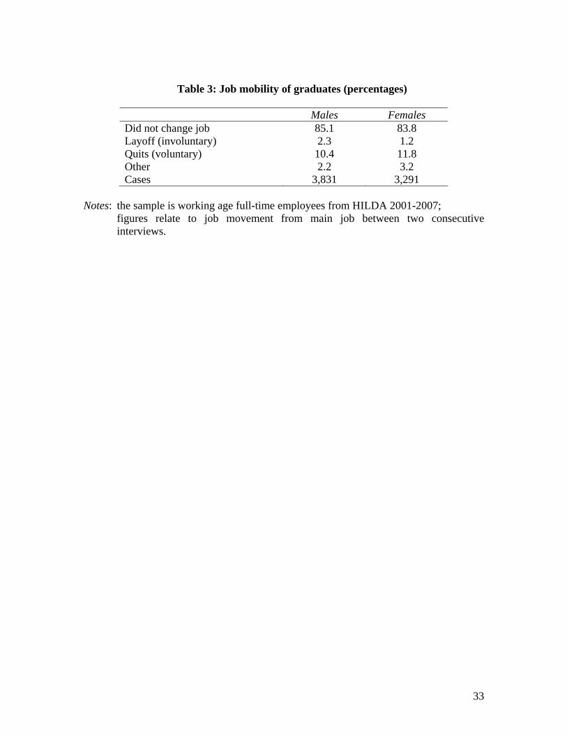
3.3.Job Mobility of Graduates by Match Type
Table 3 presents the extent of labour market mobility among our sample. HILDA records
whether respondents left their job since the last interview and the reasons underlying the
job separation. We follow McGuinness and Wooden (2009) by splitting reported job
separations into voluntary (quits), involuntary (layoffs) and other categories.5
Approximately 15 per cent of males and 16 per cent of females per annum were found to
5 Individuals were classified as having voluntarily separated if they gave any of the following as their main reason for leaving their previous employer: (i) not satisfied with job; (ii) to obtain a better job / just wanted a change / to start a new business; (iii) retired / did not want to work any longer; (iv) to stay at home to look after children, house or someone else; (v) travel / have a holiday; (vi) returned to study / started study / needed more time for study; (vii) too much travel time / too far from public transport; (viii) change of lifestyle; or (ix) immigration.

14
have left their jobs. Annual rates of voluntary separation averaged approximately 10 per
cent for men and 12 per cent for women, while layoffs were 1 or 2 per cent and
separations for other reasons 2 or 3 per cent. These patterns varied considerably when the
data was broken down by each category of mismatch. The definition of job mobility
needs to use data from two consecutive interviews and the relevant matching status is the
one reported in the first interview to reflect the way mismatch may induce mobility.
[Table 3 here]
Table 4 reveals that the incidence of voluntary separations was substantially higher
among workers who were mismatched for whatever reason than among those who were
well-matched. In this paper we are principally concerned with estimating the impact of
origin mismatch on job mobility, i.e. does mismatch increase mobility? A related
question, which we do not examine here, is the degree to which mobility may either
preserve or lead to a mismatch, i.e. does mobility eliminate mismatch?
[Table 4 here]
4. ESTIMATION METHODOLOGY
4.1 Wage Effects of Job Mismatch
To investigate the effect of job mismatch on wage, we estimate the following earnings
function:
itititit XMY εβαα +++= 0ln (1)

15
where itYln is the log of weekly earnings and itM contains three job mismatch dummy
variables as defined earlier, namely overeducated only, over skilled only and both
overeducated and overskilled for individual i at time t. X is a matrix of other relevant
personal and workplace characteristics that are used as control variables in the estimation,
including age, marital status, number of children, socioeconomic background,
unemployment history, country of origin, employment and occupational tenure, union
membership, firm size and industry.6 ε is the conventional error term. We estimate
equation (1) using a pooled OLS model on a sample of working age full-time graduate
employees, separately for male and female. The use of pooled regression is a good
starting point and benchmark for the analysis. It provides us with an overview of the
relationships we examine in terms of the cross sectional differences in the sample.
Although largely informative in a descriptive sense, pooled regression estimates are
always subject to biases due to unobserved systematic individual differences in the
sample. Thus, we also use panel estimation which controls for time invariant unobserved
individual heterogeneity and allows us to come closer to making inferences about causal
effects. The first panel estimation uses a fixed effects model, which takes the form below:
itiititit uaXMY ++++= βαα0ln (2)
where ia is the individual fixed effect and itu is the idiosyncratic error.
6 Variables are listed and explained in detail in Appendix I.
16
We also estimate the earnings equation using a random effects model augmented with a
Mundlak (1978) correction to control for unobserved time-invariant individual
heterogeneity:
itiiititit vXMXMY +++++= 210ln ξξβαα (3)
where iM and iX are the time averages of itM and itX for individual i, respectively. In
principle, the estimates of α and β in equation (3) approximate the fixed effects
(within) estimators. Unlike the fixed effects model, the random effects with Mundlak
corrections model obtains explicit estimates on the variables with little or no over time
variation within the observation period of the data.
4.2 Job Satisfaction and Job Mobility Effects of Job Mismatch
For clarity of interpretation we have converted the ordered job satisfaction variables into
binary variables. In the HILDA data job satisfaction is measured as a 0 to 10 (lowest to
highest) scale. We use a binary variable which is zero for values between 0 and 6 and is
one for values between 7 and 10. Extensive sensitivity analyses regarding the cut-off
points we use were carried out suggesting that estimation results are not sensitive on the
exact cut-off point selected. The same conversion has been applied to each job
satisfaction facet variable. The relationship between job mobility and matching models
the incidence of having moved job since the previous wave as a function of the level of
mismatch experienced in that previous wave. Thus, the question we ask in the mobility
estimations is whether mismatch influences the stability of employment. We initially
model all job separations jointly before estimating models for voluntary (quits) and
involuntary (layoffs) mobility separately.

17
Since binary variables are used for job satisfaction and job mobility, the pooled OLS and
fixed effects model become unavailable. Instead, we use both a pooled probit model and
a random effects probit model with a Mundlak correction to estimate the effect of job
mismatch on job satisfaction and job mobility, leaving the explanatory variables to be the
same as those used in the wage effects estimation.
In all, this paper uses a number of estimation methods. Each type of estimation contains
different information and the comparisons we present are informative. The use of the
pooled data serves two purposes. First, it provides a set of estimates that is comparable
with the majority of the literature estimates, where panel data methods have not been
utilised. Second, it provides a reasonable estimate of the association between labour
market outcomes and the mismatch. Pooled estimates will reflect the net association
between wages, satisfaction and mobility with mismatch, caused by all observed and
unobserved factors. By contrast, panel estimates will be much closer to the causal effects
between the dependent and independent variables, as they control for both observed and
unobserved individual heterogeneity. It is worth noting that, since the information
contained in the data is the same for both estimations, the major difference in the
estimates is that the panel estimation controls for unobserved heterogeneity, while the
pooled estimation does not. However, the panel estimates also have their limitations as
they cannot handle well the cases where there is little variation over time. We discuss
these issues below when we contrast and interpret pooled cross section with random and
fixed effects panel results.

18
5. REGRESSION RESULTS
5.1 Wage Effects of Job Mismatch
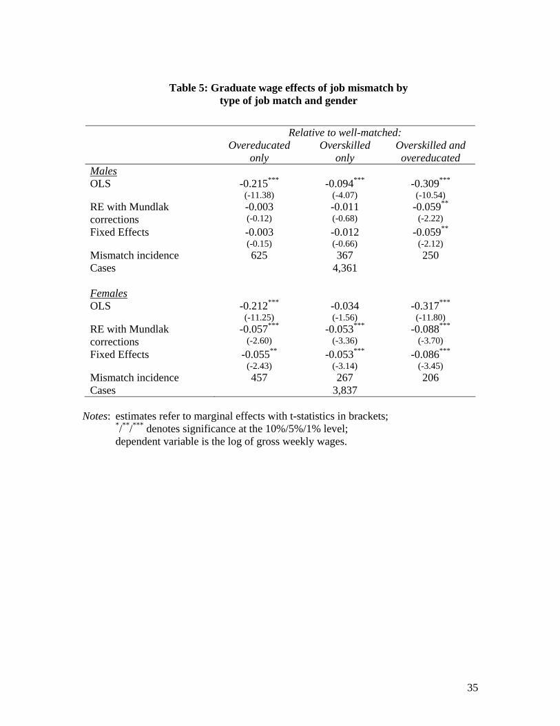
Possibly the most important and definitely the most well-researched consequence of
mismatch is the effect it may have on wages. A common result in the literature, as noted
earlier, is that mismatches are associated with lower pay, which reflects the lower
productivity of a sub-optimal worker-job match, though it must be noted that
overeducated workers do receive higher pay than their educationally appropriately
matched co-workers, suggestive of some productivity advantage to being overeducated
(see Sicherman, 1991). Table 5 shows that OLS estimation produces highly significant
coefficients in all types of mismatch. Not surprisingly, the strongest associations are
found for those who are both overeducated and overskilled. The Random Effects (RE)
model with Mundlak corrections produces, as expected, almost identical estimates as the
Fixed Effects model and in all cases much weaker estimates than the OLS pooled model.
[Table 5 here]
The first main result in Table 5 is that controlling for unobserved heterogeneity removes
most of the wage impact for men who are overeducated only or overskilled only.
Graduate men who change status from a well-matched job to an overeducated only or an
overskilled only job do not suffer a wage penalty. It is only well-matched graduate men
who change status to a job where they are both overeducated and overskilled that suffer
an approximate 5.9 per cent wage penalty.

19
It is noteworthy that the panel estimates of wage penalties due to mismatch are
substantially different from the estimates of overall association produced by the OLS
models, suggesting that unobserved systematic differences play a significant role in
determining mismatch effects. Women in full-time employment appear to suffer a wage
penalty when they change status from a well-matched to a mismatched job for all types of
mismatch. This is a significant result as it ties with the literature on discrimination which
has found that gender pay differentials are higher upon re-employment.7 When we
compare the wage penalties of both men and women we see that women suffer a worse
pay deterioration than men when changing status from a well-matched job into a
mismatched job, the differential being net of systematic differences in unobserved
individual heterogeneity.
However, there is some recent evidence to suggest that Fixed Effects estimators (and by
extension Random Effects estimates after the incorporation of Mundlak corrections) may
themselves be biased by under-estimating the true impact of some covariates in a model.
Buddelmeyer et al. (2010) suggested that fixed effects can absorb a good deal of the
explanatory power of those time-varying variables that show little variation within the
time period covered by the sample at hand. This is potentially a concern for studies of
skill mismatch, given that existing evidence suggests that both overeducation and
overskilling are relatively time-persistent states (McGuinness 2006). To investigate this
possibility, we estimate a two-stage model whereby we extract the individual level fixed
effects from a first-stage Fixed Effects estimation and use them as the dependent variable
7 Mavromaras and Rudolph (1997) estimated gender pay differentials upon re-employment using administrative data from the Federal Employment Office in Germany and found that the re-employment process is associated with an increase in gender pay differentials.

20
in a second-stage pooled OLS regression with all the time varying means of each of our
original explanatory variables (that is, the Mundlak controls) on the right hand side. The
inclusion of the Mundlak means as right-hand-side variables provides an indication of the
relative contribution of each variable (including the mismatch indicators on which this
paper focuses) to the overall fixed effect.
Table 6 reports the coefficients and t-statistics of the mismatch controls along with the
adjusted R2 of each regression. The time varying averages as right hand side variables
explain a high proportion of the overall individual level fixed effects, more so for females
as reflected in the adjusted R2 statistics. The results confirm that the variables indicating
overeducated only, overskilled only and both overskilled and overeducated account for a
proportion of the fixed effect. The negative signs suggest that the coefficients for the
Fixed Effects and the Random Effects with Mundlak corrections models reported in
Table 5 may be under-estimating (with the exception of females whose changed status to
an overskilled only job yields a positive coefficient, thus over-estimating the true impact
of the mismatch variables on wages). Table 6 results show some interesting gender
differences. The mismatch penalty for males is under-estimated for all types of mismatch,
but notably less for only overskilled males. This may not be surprising, in that
overskilling is the variable that changes most through individual job moves and thus
contains most over time variation. Interestingly, the result of under-estimated mismatch
wage penalty holds largely unchanged for females in the category of overeducated only
and both overskilled and overeducated, but is reversed for females who are overskilled
only.

21
[Table 6 here]
5.2 Overall Job Satisfaction and Mismatch
We treat job satisfaction as an outcome of mismatch by observing the effect that each
type of mismatch has on resulting job satisfaction levels after we have controlled for
other factors that may also affect job satisfaction. The interpretation of our results is that
where a mismatch does not appear to reduce job satisfaction it is more likely that this
mismatch reflects voluntary under-utilisation of skills or qualifications (or, at least if not
voluntary, not harmful according to the worker). By contrast, a mismatch that reduces job
satisfaction is more likely to reflect involuntary under-utilisation. Table 7 presents the
difference in overall job satisfaction between the well-matched and those that belong to
one of the three categories of mismatch, estimated using pooled (cross-section) probit and
Random Effects (panel) probit with Mundlak corrections.8 We report results for males
and females separately. Estimates on overeducation only (Table 7, column 1) suggest
that, once we have controlled for mismatch that is attributable to being overskilled,
mismatch attributable to being overeducated only has no discernible effect on the job
satisfaction of males and females alike. This result is in agreement with Green and Zhu’s
(2008) finding that education mismatch in itself does not lower the level of job
satisfaction.9
8 Note that we do not perform conditional probit fixed effects estimation as it is not possible to condition the fixed effects out of the likelihood function. Therefore, we report only Random Effects probit models. 9 There is a suggestion in the overeducated only results that, when we shift from cross-section to panel results (i.e. after controlling for unobserved individual heterogeneity with the RE model with Mundlak corrections) a small dissatisfaction effect arises, as the magnitude of estimates rise, especially for females. However, their statistical significance remains well below acceptable levels. One possible explanation would have been that a sub-group among females would respond differently to overskilling. We examined a number of sample splits, including one between married and single females, but could find no such pattern in the overskilling-job satisfaction relationship.

22
[Table 7 here]
Estimates on overskilled only (Table 7, column 2) suggest that overskilling can be a
prime cause of lower job satisfaction, with some gender differences present. For males,
controlling for unobserved heterogeneity in the estimation leads to considerable reduction
in the job satisfaction negative effect, more than halving the marginal effect (from -0.685
to -0.328). This difference between the two estimates implies that unobserved
heterogeneity introduces a negative bias on the effect of mismatch on job satisfaction,
which would suggest that male employees of a generally unhappy disposition towards
work are more likely to end up in jobs that under-utilise their skills, for reasons that are
not explained by our data. This pattern is repeated for males who are both overeducated
and overskilled. For females, controlling for unobserved heterogeneity has a hardly
discernible effect (from -0.661 to -0.625), which suggests that females with a generally
unhappy disposition towards work are equally likely to end up in an overskilled only job
as their happier counterparts. Females end up with the same reduction in job satisfaction
as males when they move from a well-matched job to a job where they are both
overeducated and overskilled (panel estimate is -0.621 for males and -0.622 for females),
but unlike males, controlling for unobserved heterogeneity increases their dis-satisfaction
(from -0.380 to -0.622), indicating that unobserved heterogeneity bias works in the
opposite direction for males and females. This implies that, although we find that the
generally happier females are more likely to end up in the both overeducated and
overskilled category than their male counterparts, the dis-satisfaction caused by ending up
in such a job is equally strong for both males and females (-0.621 for males and -0.622
for females). In conclusion, estimates of the comparison between those who are well-

23
matched with those who happen to be both overskilled and overeducated (Table 7,
column 3) clearly suggest that even after we have controlled for all available observable
attributes and all time invariant unobservable attributes, job satisfaction can be still
shown to be seriously damaged by this type of severe mismatch. Our results clearly do
not contradict those of Green and Zhu regarding the importance of combined overskilling
and overeducation.
5.3 Facets of Job Satisfaction and Job Mismatch
The data contain detailed information about the degree of satisfaction regarding several
facets of employment, namely, pay, job security, work, hours and flexibility. Estimation
results by gender for all job satisfaction facets are in Table 8. The first row reported for
each gender in Table 8 is the estimate of overall job satisfaction (already reported in
Table 7) and the rows that follow report the facets of job satisfaction. A similar picture
arises to the one for overall job satisfaction in that being overeducated only does not have
an impact on satisfaction (with the exception of hours dis-satisfaction by overeducated
males). Table 8 suggests that for the overskilled only the only facet that is consistently
statistically significant is that of work satisfaction, which is bound to be a closely related
to the overall satisfaction variable. It is possible that, empirically, these two variables are
not as clearly distinguishable from one another as we would like them to be. It is worth
noting, however, that for both males and females the work satisfaction estimates are
stronger than the overall job satisfaction ones. The marginal effects of being overskilled
only in the pay satisfaction estimation have a statistical significance close to the 10
percent level, positive for males (with a t-ratio of 1.64) and negative for females (with a t-
ratio of -1.57, very near the margin of the 10% significance level). The implication here

24
is that men who change status from well-matched to overskilled only jobs tend to be more
satisfied with their pay. Note that this conclusion is in agreement with the estimated wage
penalties where we find no wage penalty for overskilled only males and a small penalty
for females. Moving to workers that are both overskilled and overeducated, we note that
dis-satisfaction with work is clearly present and that there is clear hours dis-satisfaction
for males and job security dis-satisfaction for females.
[Table 8 here]
5.4 Job Mobility and Job Mismatch
Job separations have been argued to be a consequence of inadequate matches
(McGuinness and Wooden, 2009). It is useful to distinguish between voluntary
separations (quits initiated by the employee) from involuntary separations (layoffs
initiated by the employer), although we should bear in mind that, in practice, there will be
occasions where this decision will be endogenous. Thus, voluntary mobility is more
likely to reflect dissatisfaction expressed by the employee, while involuntary mobility is
more likely to reflect dissatisfaction expressed by the employer. We estimate the
probability of an individual changing jobs between two consecutive interviews depending
on their level of mismatch in the job that they left (denoted as “in origin job” in Table 9),
in order to examine if employees who are mismatched in their job are more or less likely
to quit or be laid off than their well-matched counterparts. We maintain the same
estimation methodology and specification and compare a pooled (cross section) probit
with a Random Effects probit model with Mundlak corrections, separating our sample by
gender.

25
Table 9 contains estimation results on job mobility by type of mobility and gender. The
first clear message is that, after we have controlled for individual unobserved
heterogeneity, neither of the three categories of mismatch has any significant effect on
involuntary job mobility and it is just overeducation on its own or jointly with
overskilling that increases voluntary mobility, and then only for males. The general lack
of a significant direct effect of mismatch on mobility appears to be in contrast to other
published work which has typically been either based on cross section estimation or short
panel data. It is worth noting that the pooled probit models in Table 9, which contain
many statistically significant estimates of mismatch (especially male layoffs), lose their
significance when we use panel estimation. This suggests that some of that significance
was caused by unobserved heterogeneity bias. Note that we reached a similar conclusion
in the wage estimations after controlling for unobserved heterogeneity. Notwithstanding
this evidence, we think the issue of job mobility and mismatch remains unclear,
principally because we fail to control for employer-specific unobserved heterogeneity,
which we would expect to be pertinent in the case of layoffs.
[Table 9 here]
The comparison between the pooled probit and the Random Effects probit with Mundlak
corrections has an important interpretation in this context: given that the pooled results do
not control for unobserved individual heterogeneity, while the random effects estimates
do, the differences between the two sets of estimates contain information about the
association between unobserved heterogeneity and the dependent variable. Following a

26
similar line of argument as with the wage penalties and using the case of overeducated
only males as an example, we see a very different pattern between quits and layoffs.
Removing the effect of unobserved individual characteristics reduces the marginal effect
from 0.112 to -0.029 for layoffs and increases it from -0.063 to 0.438 for quits, which
means that using pooled regression over-estimates the effect of overeducation on layoffs
and under-estimates its effect on quits for males. Put simply, our mobility regressions
suggest that overeducated only males possess some unobserved characteristics which
increase their probability of quitting and decrease their probability of being laid off.
Similar comparisons can be made for the remaining estimates in Table 9 and they show
no clear pattern by type of mismatch or by gender.
6. CONCLUSIONS
The earlier literature on graduate mismatch found that there were both pay and job
satisfaction penalties to being overqualified, but most of this literature was constrained by
the unavailability of data on overskilling and also by the absence of panel data which
would have allowed for controls on unobserved individual heterogeneity, such as
variations in innate ability or employability. Our data relate to only one country, namely
Australia, but the use of the panel element of HILDA and the presence of a question on
overskilling enables us to put a new perspective on earlier results from a variety of
countries.
In this paper we have introduced a more detailed definition of worker-job mismatch than
contained in the earlier literature with a mismatched worker being analysed according to
whether he or she is either overeducated, overskilled or a combination of the two. We

27
present two types of estimations: pooled cross-section regression and random effects
probit with Mundlak corrections. Pooled regressions can be informative about the overall
association between labour market outcomes and mismatch, while random effects
estimates give us a measure of the possible causal effect of mismatch on labour market
outcomes. We have estimated a large number of models to establish the repercussions of
labour market mismatch in terms of individual wages, job satisfaction and job mobility.
We also carried out the analysis separately for males and females. In general, the data
support the view that overeducation and overskilling are distinct phenomena, that they
work differently by gender, that they have a different effect on different labour market
outcomes and that the negative effects of being both overeducated and overskilled are
more severe.
Our results differ from the earlier literature in a number of respects. First, for men we
find there to be a significant pay penalty only for those who are both overskilled and
overeducated, while for women there is a significant pay penalty in all cases of mismatch.
Second, for both genders job satisfaction is not influenced by overeducation, but it is
clearly reduced by overskilling either on its own or jointly with overeducation. Thus
overskilling appears to be more welfare reducing than overeducation. For many,
overeducation is a matter of choice or necessity, whereas overskilling is a matter of
regret. We obtain little further insight when we estimate the facets of job satisfaction
instead of a measure of overall job satisfaction. Third, in the case of quits, with the
exception of overeducation on its own and jointly with overskilling for males, mismatch
has no significant effect on the job mobility of either gender. Finally, a core result of this
paper is that it shows the very important role played by properly controlling for

28
unobserved heterogeneity when estimating the labour market outcomes of mismatch: past
results based on cross section and short panel data sets are shown to contain considerable
biases.
The results suggest that it is on overskilling and particularly its combination with
overeducation that policy attention should be focused. Since overeducation has no clearly
negative effect on the welfare of either men or women, its occurrence should not be a
matter of major policy concern. However, overskilling whether on its own or jointly with
overeducation does so and its eradication may have benefits for employers as well as
employees. It is particularly interesting that the wage penalty of mismatch is higher for
females and so is their reported dissatisfaction caused by mismatch, especially so by
overskilling. Mismatch appears to be more damaging for females.

29
REFERENCES
Allen, J. and van der Velden, R. (2001). “Education Mismatches Versus Skill Mismatches: Effects on Wages, Job Satisfaction, and On-the-Job Search,” Oxford Economic Papers, 53, 434-452.
Bauer T. (2002), “Educational Mismatch and Wages: A Panel Analysis”, Economics of Education Review, 21, 221-229.
Belfield C. (2010), “Over-education: What Influence Does the Workplace Have?”, Economics of Education Review, 29, 236-245.
Buddelmeyer H., Lee W-S. and Wooden M. (2010), “Low-Paid Employment and Unemployment Dynamics in Australia”, Economic Record, 86(272), 28-48.
Chevalier A. (2003), “Measuring Overeducation”, Economica, 70(209), 509-531.
European Commission (2009), New Skills for New Jobs; Anticipating and Matching Labour Market and Skill Needs, Luxembourg.
Freeman R.B. (1978), The Overeducated American, Academic Press.
Green F. and McIntosh S. (2007), “Is There a Genuine Under-utilization of Skills amongst the Over-qualified?”, Applied Economics, 39(4), 427-439.
Green F. and Zhu Y.(2008), “Overqualification, Job Dissatisfaction, and Increasing Dispersion in the Returns to Graduate Education”, University of Kent Department of Economics Discussion Paper KDPE 0803.
Kler, P. (2005), “Graduate Overeducation in Australia: A Comparison of the Mean and Objective Methods”, Education Economics, 13, 47-72.
Kler P. (2006), “The Impact of Overeducation on Job Satisfaction Among Tertiary Educated Australians”, unpublished manuscript, University of Queensland.
Kler P. (2007), “A Panel Data Investigation into Over-education among Tertiary Educated Australian Immigrants”, Journal of Economic Studies, 34(3), 179-193.
Lindley J. and McIntosh S.(2008),”A Panel Analysis of the Incidence and Impact of Overeducation”, Department of Economics, University of Sheffield, July.
Mavromaras, K., McGuinness, S. and Fok Y.K. (2009). “Assessing the Incidence and Wage Effects of Overskilling in the Australian Labour Market”, Economic Record, 85(268), 60-72.

30
Mavromaras, K., McGuinness, S., O’Leary, N., Sloane, P. and Y. K. Fok (2010) “The Problem of Overskilling in Australia and Britain.” The Manchester School, 40(3), 219-241.
Mavromaras, K., and Rudolph, H. (1997), "Wage Discrimination in the Reemployment Process." Journal of Human Resources 32(4), 812-860.
McGuinness S. (2006) “Overeducation in the Labour Market”. Journal of Economic Surveys 20, 387–418.
McGuinness, S. and Wooden, M.(2009), “Overskilling, Job Insecurity and Career Mobility”, Industrial Relations, Vol. 48(2), 265-286.
Mundlak Y.(1978), “On the Pooling of Time Series and Cross Section Data”, Econometrica, 46(1), 69-85.
Sicherman N. (1991), “Overeducation in the Labor Market,” Journal of Labor Economics, 9(2), 101-122.
Tsai Y .(2010), “Returns to Overeducation: A Longitudinal Analysis of the U.S. Labor Market, Economics of Education Review, doi:10.1016/j.econedurev.2010.01.001.
Watson, N. and Wooden, M. (2004), “The HILDA Survey Four Years On”, Australian Economic Review, 37(3), 343-349.

31
Table 1: Wages of graduates by type of job match
Males Females Well-matched 1537.4 1102.8 Overeducated only 1161.0 883.0 Overskilled only 1322.9 1011.7 Overskilled and overeducated 910.9 711.3
Notes: the sample is working age full-time employees from HILDA 2001-2007; wages are measured as nominal gross weekly wages and salary from main job in Australian dollars.

32
Table 2: Overall job satisfaction (percentage) of graduates by type of job match and gender
Job satisfaction
Well- matched
Overeducated only
Overskilled only
Overskilled and overeducated
M F M F M F M F 0 0.1 0.1 0.5 1.1 0.0 0.0 0.4 1.0 1 0.2 0.3 0.5 0.7 0.3 0.4 1.2 1.5 2 0.5 0.5 2.5 0.7 1.1 0.7 4.4 0.0 3 1.2 1.5 4.1 5.2 1.6 0.7 2.4 3.9 4 1.8 1.4 4.1 4.9 1.8 1.8 8.4 1.0 5 4.2 5.4 10.4 12.4 2.7 5.0 12.0 12.1 6 7.7 8.8 15.3 14.6 8.5 11.6 17.2 11.7 7 23.9 22.1 30.0 27.3 21.8 19.7 27.6 29.1 8 36.2 33.0 23.2 22.1 34.7 34.6 18.0 24.8 9 20.1 21.2 7.6 8.2 19.0 18.8 6.8 13.1 10 4.0 5.5 1.9 2.6 8.5 6.8 1.6 1.9 Total 100.0 100.0 100.0 100.0 100.0 100.0 100.0 100.0 Mean job satisfaction 7.6 7.6 7.7 7.6 6.6 6.6 6.3 6.9 Cases 3,119 2,906 625 457 367 267 250 206 Note: the sample is working age full-time employees from HILDA 2001-2007.
33
Table 3: Job mobility of graduates (percentages)
Males Females Did not change job 85.1 83.8 Layoff (involuntary) 2.3 1.2 Quits (voluntary) 10.4 11.8 Other 2.2 3.2 Cases 3,831 3,291
Notes: the sample is working age full-time employees from HILDA 2001-2007; figures relate to job movement from main job between two consecutive interviews.

34
Table 4: Job mobility of graduates (percentages) by type of job match in the first interview and gender
Males Well-
matched Overeducated
only Overskilled
only Overskilled and overeducated
Did not change job 89.6 84.6 83.0 74.5 Layoff (involuntary)
1.4 3.2 4.5 4.6
Quits (voluntary) 7.5 10.8 11.1 16.8 Other 1.5 1.3 1.4 4.1 Females Well-
matched Overeducated
only Overskilled
only Overskilled and overeducated
Did not change job 88.3 87.7 76.0 81.7 Layoff (involuntary)
1.2 0.6 2.6 0.0
Quits (voluntary) 8.8 10.7 15.1 13.7 Other 1.7 1.0 6.3 4.6
Notes: the sample is working age full-time employees from HILDA 2001-2007; figures relate to job movement from main job between two consecutive interviews; job mobility is defined as a change in jobs between consecutive interviews; matching status defined as that reported in the first of the two interviews.
35
Table 5: Graduate wage effects of job mismatch by type of job match and gender
Relative to well-matched: Overeducated
only Overskilled
only Overskilled and overeducated
Males OLS -0.215***
(-11.38) -0.094***
(-4.07) -0.309***
(-10.54) RE with Mundlak corrections
-0.003 (-0.12)
-0.011 (-0.68)
-0.059** (-2.22)
Fixed Effects -0.003 (-0.15)
-0.012 (-0.66)
-0.059** (-2.12)
Mismatch incidence 625 367 250 Cases 4,361 Females OLS -0.212***
(-11.25) -0.034 (-1.56)
-0.317*** (-11.80)
RE with Mundlak corrections
-0.057*** (-2.60)
-0.053*** (-3.36)
-0.088*** (-3.70)
Fixed Effects -0.055** (-2.43)
-0.053*** (-3.14)
-0.086*** (-3.45)
Mismatch incidence 457 267 206 Cases 3,837
Notes: estimates refer to marginal effects with t-statistics in brackets; */**/*** denotes significance at the 10%/5%/1% level; dependent variable is the log of gross weekly wages.

36
Table 6: Impact of job mismatch on individual fixed effects by type of job match and gender
Relative to well-matched: Overeducated
only Overskilled
only Overskilled and overeducated
Males Fixed Effect – OLS -0.316***
(-15.83) -0.117***
(-4.13) -0.324***
(-10.23) Adjusted R2 0.79 0.79 0.79 Female s
Fixed Effect – OLS -0.241*** (-11.86)
0.066** (2.51)
-0.323*** (-11.86)
Adjusted R2 0.83 0.83 0.83 Notes: estimates refer to marginal effects with t-statistics in brackets; */**/*** denotes significance at the 10%/5%/1% level.

37
Table 7: Overall job satisfaction for graduates by type of job match and gender
Relative to well-matched:
Overeducated only
Overskilled only
Overskilled and overeducated
Males Pooled probit 0.027
(0.36) -0.685***
(-8.81) -0.877***
(-8.96) RE probit (with Mundlak corrections)
-0.077 (-0.57)
-0.328*** (-2.76)
-0.621*** (-3.49)
Females Pooled probit -0.024
(-0.28) -0.661***
(-7.58) -0.380***
(-3.38) RE probit (with Mundlak corrections)
-0.225 (-1.44)
-0.625*** (-4.58)
-0.622*** (-2.84)
Notes: estimates refer to marginal effects with t-statistics in brackets; */**/*** denotes significance at the 10%/5%/1% level; job satisfaction cut-off point at 7.

38
Table 8: Job satisfaction facets for graduates by
type of job match and gender
Relative to well-matched: Overeducated
only Overskilled
only Overskilled and overeducated
Males Overall job satisfaction -0.077
(-0.57) -0.328***
(-2.76) -0.621***
(-3.49) Pay satisfaction 0.041
(0.32) 0.200 (1.64)
-0.078 (-0.45)
Job security satisfaction 0.183 (1.33)
-0.077 (-0.57)
0.066 (0.35)
Work satisfaction 0.053 (0.39)
-0.533*** (-4.53)
-0.604*** (-3.49)
Hours satisfaction -0.206* (-1.66)
-0.167 (-1.40)
-0.442** (-2.44)
Flexibility satisfaction 0.077 (0.59)
-0.033 (-0.27)
-0.147 (-0.82)
Females Overall job satisfaction -0.225
(-1.44) -0.625***
(-4.58) -0.622***
(-2.84) Pay satisfaction -0.090
(-0.64) -0.210 (-1.57)
-0.103 (-0.49)
Job security satisfaction -0.194 (-1.17)
-0.147 (-0.89)
-0.415* (-1.72)
Work satisfaction -0.079 (-0.49)
-0.870*** (-6.31)
-1.17*** (-5.34)
Hours satisfaction 0.089 (0.58)
0.152 (1.08)
-0.304 (-1.36)
Flexibility satisfaction 0.036 (0.25)
-0.036 (-0.26)
-0.062 (-0.29)
Notes: estimates refer to marginal effects with t-statistics in brackets; */**/*** denotes significance at the 10%/5%/1% level; job satisfaction cut-off point at 7; estimation is by Random Effects Probit with Mundlak correction using the same specification as in Table 7; for reasons of space cross section results are not reported.

39
Table 9: Effects of job mismatch on graduate job mobility by type of job match and gender
Relative to well-matched: Type of job loss Overeducated
only (lagged) Overskilled
only (lagged) Overskilled and overeducated
(lagged) Males Job change (all causes) Pooled probit -0.054
(-0.41) 0.098 (0.63)
0.445** (2.55)
RE probit (with Mundlak corrections)
0.216 (1.03)
0.044 (0.21)
0.497* (1.83)
Layoffs (involuntary) Pooled probit 0.112
(0.54) 0.610***
(2.65) 0.553* (1.93)
RE probit (with Mundlak corrections)
-0.029 (-0.08)
0.377 (1.03)
0.359 (0.70)
Quits (voluntary) Pooled probit -0.063
(-0.44) -0.125 (-0.72)
0.271 (1.47)
RE probit (with Mundlak corrections)
0.438* (1.85)
-0.066 (-0.28)
0.593** (1.98)
Females Job change (all causes) Pooled probit -0.253*
(-1.77) 0.234 (1.51)
-0.323 (-1.54)
RE probit (with Mundlak corrections)
-0.245 (-1.06)
0.364* (1.66)
-0.179 (-0.47)
Layoffs (involuntary) Pooled probit -0.878
(-1.18) -0.021 (-0.03) -
RE probit (with Mundlak corrections) - - - Quits (voluntary) Pooled probit -0.164
(-1.16) 0.102 (0.68)
-0.277 (-1.36)
RE probit (with Mundlak corrections)
-0.276 (-1.19)
0.102 (0.47)
-0.271 (-0.72)
Notes: estimates refer to marginal effects with t-statistics in brackets; */**/*** denotes significance at the 10%/5%/1% level; - denotes insufficient observations to support estimation.

40
APPENDIX I
Table A1 presents the incidence of the various categories of mismatch across each of the
seven waves of HILDA. There is little evidence of any consistent pattern in the data in
terms of rising or falling rates of mismatch. Table A2 presents the distribution of the job
satisfaction by gender and wave. Table A3 presents sample descriptives.
Table A1: Graduate overeducation and overskilling (percentage) by wave and gender
Wave 1 Wave 2 Wave 3 Wave 4 Wave 5 Wave 6 Wave 7
M F M F M F M F M F M F M F Well matched
Per cent 73 79 68 77 72 73 72 74 71 76 73 75 71 76Cases 462 429 415 379 437 384 450 382 457 423 464 442 434 468
Overeducated only Per cent 13 10 14 11 13 14 13 13 15 13 14 11 18 12Cases 83 55 82 56 80 71 83 65 98 71 89 67 110 72
Overskilled only Per cent 8 6 11 6 8 8 8 8 9 6 8 7 7 7Cases 51 35 67 31 48 41 53 41 56 32 49 43 43 44
Overskilled and overeducated Per cent 6 4 7 6 7 6 6 5 5 5 5 7 5
5Cases 35 23 42 29 40 29 39 28 32 28 34 39 28 30
Total 100 100 100 100 100 100 100 100 100 100 100 100 100 100
Cases 631 542 606 495 605 525 625 516 643 554 636 591 615 614Note: sample is working age full-time employees from HILDA 2001-2007.

41
Table A2: Job satisfaction (percentage) of graduates by wave and gender
Wave 1 Wave 2 Wave 3 Wave 4 Wave 5 Wave 6 Wave 7 JS (job satisfaction)
M F M F M F M F M F M F M F
0 0 1 0 0 0 0 0 0 0 0 0 0 0 0 1 0 1 0 1 1 0 0 1 0 0 1
1 0 0 2 1 1 1 1 1 1 1 1 1 1 0 0 1 1 3 3 2 1 2 2 2 2 2 1 2 1 1 1 2 4 2 2 3 2 3 2 3 2 3 2 2 1 2 2 5 5 8 6 7 6 6 6 6 4 5 4 5 4 6 6 10 9 10 10 9 9 7 9 9 10 10 10 7 11 7 25 20 27 23 23 25 23 24 24 25 25 23 24 22 8 30 29 28 30 33 30 38 30 36 34 35 35 37 32 9 18 21 18 18 18 20 16 20 17 17 19 18 19 20 10 6 7 4 7 4 4 4 5 5 4 3 6 4 4 Total 100 100 100 100 100 100 100 100 100 100 100 100 100 100 Mean JS 7.4 7.4 7.3 7.4 7.3 7.4 7.4 7.4 7.5 7.4 7.5 7.5 7.6 7.4 Cases 688 572 674 562 658 567 669 559 711 609 701 643 695 692
Note: sample is working age full-time employees from HILDA 2001-2007.

42
Definition of Variables: Wage: Log of current weekly gross wages & salary from the main job. Overall job satisfaction: Dummy variable, takes the value 1 if overall job satisfaction is 7 or above, zero if 0 to 6. Facets of job satisfaction: Pay satisfaction, job security satisfaction, work satisfaction, hours satisfaction and flexibility satisfaction are defined in the same way as overall job satisfaction. Job mobility: Job loss: Dummy variable, takes the value 1 if an individual has job loss between two consecutive interviews, zero otherwise. Lay offs (Involuntary job loss): Dummy variable, takes the value 1 if an individual has involuntary job loss between two consecutive interviews, zero otherwise. Quits (voluntary job loss): Dummy variable, takes the value 1 if an individual has voluntary job loss between two consecutive interviews, zero otherwise. Mismatch variables: Overeducated Only: Dummy variable, takes the value 1 if an individual is overeducated only, zero otherwise. Overskilled Only: Dummy variable, takes the value 1 if an individual is overskilled only, zero otherwise. Overskilled and overeducated: Dummy variable, takes the value 1 if an individual is overskilled and overeducated, zero otherwise. Well matched is the reference category. Age: Continuous variable, expressed in years. Age Square: Continuous variable, expressed in years. Married: Dummy variable, takes the value 1 if an individual is married (or de facto), zero otherwise. Urban: Dummy variable, takes the value 1 if an individual domiciled within a major city, zero otherwise. Father was a professional: Dummy variable, takes the value 1 if father belonged to a professional occupation, zero otherwise.

43
Country of birth: Migrant (English speaking country): Dummy variable, takes the value 1 if migrant from an English speaking country, zero otherwise. Migrant (non-English speaking country): Dummy variable, takes the value 1 if migrant from a non English speaking country, zero otherwise. Australian born is the reference category. Hours per week usually worked in main job: Continuous variable, expressed in hours. Tenure in the current occupation: Continuous variable, expressed in years. Firm size: Less than 5 employees: Dummy variable, takes the value 1 if working in a firm which has less than 5 employees, zero otherwise. 5 to 9 employees: Dummy variable, takes the value 1 if working in a firm which has 5 to 9 employees, zero otherwise. 10 to 19 employees: Dummy variable, takes the value 1 if working in a firm which has 10 to 19 employees, zero otherwise. 20 to 49 employees: Dummy variable, takes the value 1 if working in a firm which has 20 to 49 employees, zero otherwise. More than 49 employees is the reference category. Children aged between 5 and 14: Dummy variable, takes the value 1 if an individual has children between the ages of 5 and 14, zero otherwise. Children aged under 5: Dummy variable, takes the value 1 if an individual has children aged under 5, zero otherwise. Percent time spent unemployed in last financial year: Continuous variable, value of which lies between 0 and 100. Union member: Dummy variable, takes the value 1 if an individual is a member of a trade union, zero otherwise. Sector: Agriculture, forestry and fishing: Dummy variable, takes the value 1 if working in the industry of agriculture, forestry and fishing, zero otherwise.

44
Mining: Dummy variable, takes the value 1 if working in the industry of mining, zero otherwise. Electricity, gas, water and waste services: Dummy variable, takes the value 1 if working in the industry of electricity, gas, water and waste services, zero otherwise. Construction: Dummy variable, takes the value 1 if working in the industry of construction, zero otherwise. Wholesale trade: Dummy variable, takes the value 1 if working in the industry of wholesale trade, zero otherwise. Retail trade: Dummy variable, takes the value 1 if working in the industry of retail trade, zero otherwise. Accommodation and food services: Dummy variable, takes the value 1 if working in the industry of accommodation and food services, zero otherwise. Transport, postal and warehousing: Dummy variable, takes the value 1 if working in the industry of transport, postal and warehousing, zero otherwise. Information media and telecommunications: Dummy variable, takes the value 1 if working in the industry of information media and telecommunications, zero otherwise. Financial and insurance services: Dummy variable, takes the value 1 if working in the industry of financial and insurance services, zero otherwise. Rental, hiring and real estate services: Dummy variable, takes the value 1 if working in the industry of rental, hiring and real estate services, zero otherwise. Professional, scientific and technical services: Dummy variable, takes the value 1 if working in the industry of professional, scientific and technical services, zero otherwise. Administrative and support services: Dummy variable, takes the value 1 if working in the industry of administrative and support services, zero otherwise. Public administration and safety: Dummy variable, takes the value 1 if working in the industry of public administration and safety, zero otherwise. Education and training: Dummy variable, takes the value 1 if working in the industry of education and training, zero otherwise. Health care and social assistance: Dummy variable, takes the value 1 if working in the industry of health care and social assistance, zero otherwise. Arts and recreation services: Dummy variable, takes the value 1 if working in the industry of arts and recreation services, zero otherwise. Other services: Dummy variable, takes the value 1 if working in the industry of other services, zero otherwise. Manufacturing is the reference category.

45
Table A3: Descriptive statistics
Explanatory variable Males Females Age 39.517 (10.067) 37.514 (10.510) Age Square 1662.9 (818.2) 1517.7 (817.9) Married 0.785 0.641 Urban 0.935 0.917 Father was a professional 0.276 0.265 Migrant (English speaking country) 0.131 0.105 Migrant (non-English speaking country) 0.146 0.139 Hours per week usually worked in main job 45.784 (8.669) 42.876 (8.056) Tenure in the current occupation 9.486 (9.172) 8.786 (9.215) Tenure with current employer 7.615 (8.416) 6.682 (7.602) Firm has less than 5 employees 0.044 0.038 Firm has 5 to 9 employees 0.061 0.066 Firm has 10 to 19 employees 0.098 0.089 Firm has 20 to 49 employees 0.177 0.193 Have children aged between 5 and 14 0.284 0.188 Have children aged under 5 0.175 0.052 Percent time spent unemployed in last financial year 0.816 (5.411) 1.243 (7.428) Union member 0.316 0.458 Agriculture, forestry and fishing 0.015 0.006 Mining 0.023 0.003 Electricity, gas, water and waste services 0.015 0.005 Construction 0.031 0.004 Wholesale trade 0.028 0.014 Retail trade 0.037 0.024 Accommodation and food services 0.006 0.006 Transport, postal and warehousing 0.024 0.009 Information media and telecommunications 0.038 0.040 Financial and insurance services 0.074 0.041 Rental, hiring and real estate services 0.014 0.004 Professional, scientific and technical services 0.160 0.102 Administrative and support services 0.011 0.017 Public administration and safety 0.134 0.102 Education and training 0.195 0.327 Health care and social assistance 0.064 0.238 Arts and recreation services 0.017 0.015 Other services 0.020 0.013 Note: Mean (standard deviation). The sample consists of all working age full-time graduate employees from HILDA 2001-2007, and includes 4361 males and 3837 females.