DI

SC

US

SI

ON

P

AP

ER

S

ER

IE

S

Forschungsinstitut zur Zukunft der ArbeitInstitute for the Study of Labor

Job Loss and Regional Mobility

IZA DP No. 8780

January 2015

Kristiina HuttunenJarle MøenKjell G. Salvanes

Job Loss and Regional Mobility

Kristiina Huttunen Aalto University School of Economics

and IZA

Jarle Møen Norwegian School of Economics

Kjell G. Salvanes

Norwegian School of Economics, CEE (CEP), CEPR and IZA

Discussion Paper No. 8780 January 2015

IZA

P.O. Box 7240 53072 Bonn

Germany

Phone: +49-228-3894-0 Fax: +49-228-3894-180

E-mail: iza@iza.org

Any opinions expressed here are those of the author(s) and not those of IZA. Research published in this series may include views on policy, but the institute itself takes no institutional policy positions. The IZA research network is committed to the IZA Guiding Principles of Research Integrity. The Institute for the Study of Labor (IZA) in Bonn is a local and virtual international research center and a place of communication between science, politics and business. IZA is an independent nonprofit organization supported by Deutsche Post Foundation. The center is associated with the University of Bonn and offers a stimulating research environment through its international network, workshops and conferences, data service, project support, research visits and doctoral program. IZA engages in (i) original and internationally competitive research in all fields of labor economics, (ii) development of policy concepts, and (iii) dissemination of research results and concepts to the interested public. IZA Discussion Papers often represent preliminary work and are circulated to encourage discussion. Citation of such a paper should account for its provisional character. A revised version may be available directly from the author.

IZA Discussion Paper No. 8780 January 2015

ABSTRACT

Job Loss and Regional Mobility* It is well documented that displaced workers suffer severe earnings losses, but not why this is so. One reason may be that workers are unable or unwilling to move to regions with better employment opportunities. We study this and find that job displacement increases regional mobility but, surprisingly, we also find that displaced workers who move suffer larger income losses than displaced workers who stay in the same region. This is not a selection effect, but reflects the fact that non-economic factors such as family ties are very important for the decision to migrate. Workers are less likely to move if they have family in the region where they already live, and job loss stimulates workers to relocate with parents and siblings when they live in different regions. Looking at earnings we find that the entire post displacement income difference between displaced movers and stayers is driven by workers moving to regions where their parents live or to rural areas. Furthermore, when looking at long-run family income, we find that the difference between displaced movers and stayers is very modest. With respect to selection, we find that migrants are positively selected on average, but very heterogeneous. They seem to be drawn disproportionately both from the high and the low end of the skill distribution in the region they leave. JEL Classification: J61, J63 Keywords: plant closures, downsizing, regional mobility, earnings, family ties Corresponding author: Kristiina Huttunen Aalto University School of Economics P.O. Box 21240 00076 Aalto Finland E-mail: kristiina.huttunen@aalto.fi

* We thank Matti Sarvimäki and seminar participants at the Norwegian School of Economics, in Austin and Jyväskylä, and participants at the SOLE and EALE meetings in Washington and Ljubliana. Huttunen gratefully acknowledges financial support from the Finnish Academy. Salvanes and Møen thank The Norwegian Research Council for financial support.

1

1 Introduction

One of the long-standing puzzles in economics is why there are persistent differences in

employment and earnings across regions (Blanchard and Katz, 1992). Why do the workers

simply not relocate? Another question that is not well understood, is why workers who have lost

their jobs in plant closures or mass layoff events suffer significant and long-lasting employment

and earnings losses.1 One possible explanation for both these puzzles is that workers are

immobile and therefore face restrictions in their job search. The costs of moving may vary due to

family commitments, networks and preferences regarding local amenities. Understanding the

factors that determine migration is important for policy makers when they develop policies for

regions that face adverse economic shocks.2 While the literature on both migration and job

displacement is large, we know little specifically about the migration behavior of displaced

workers and how they fare in the labor market. This paper aims to fill this gap in the literature by

analyzing the mobility behavior and earnings of workers that have lost their jobs in plant closures

or mass layoffs in Norway.

Plant exits and downsizing are considered an exogenous transitory income and employment

shock to the individual workers. Our analysis consists of two parts. In the first part we analyze

how job displacement affects workers’ mobility decisions and what determines selection into

mobility after a job loss. Specifically, we assess the effect of family networks (siblings and

1 See e.g. Jacobsen, LaLonde and Sullivan (1994), Couch and Placzek (2010), Eliasson and Storrie (2006), Schmieder, von Wachter and Bender (2009), Rege, Telle and Votruba (2009) and Huttunen, Møen and Salvanes (2011). 2 Increased international trade with low cost countries such as China, has had a particularly big impact on downsizing and restructuring of the manufacturing sector during the last couple of decades. See Author, Dorn, and Hanson (2013) for an analysis of the impact on regional labor markets in the US, and Balsvik, Jensen, and Salvanes (2014) for an analysis of the impact in Norway. Smoothing these restructuring processes is high on policy makers’ agenda.

2

parents) in the local labor market in which the workers lose their jobs.3 Parents may affect

mobility for several reasons: People in general enjoy the company of their family, parents may

influence workers’ employment and earnings directly through their networks, parents may help

bring up grandchildren or parents may be elderly and in need of care. 4 For much the same

reasons siblings also represent a positive incentive for co-location, but having siblings can also

make it easier to move away from elderly parents because they are substitute caretakers.5

In the second part of the analysis we assess the post-displacement labor market experience of

movers and stayers. We compare displaced movers and stayers with a control group of non-

displaced workers using the standard framework. In addition, we extend this framework with a

fixed effects model borrowed from regional economics and cross-country migration studies (see

e.g. Glaeser and Mare, 2001). We analyze individual and family earnings as well as individual

and family income. Importantly, we use a regional consumer price index to take into account the

fact that living expenses (especially housing) differ across regional labor markets. Our aim in this

part of the paper is to understand whether the earnings differential between displaced movers and

stayers is a causal effect of moving and whether movers tend to be positively or negatively

selected.

It is not clear how workers select into migration after permanent job loss. While a standard

proposition in the migration literature is that migrants tend to be favorably self-selected, it may

3 It is well established that family ties influence workers’ mobility decisions (Mincer, 1978). Alessina et al. (2010) show that individuals who inherit stronger family ties are less mobile, have lower wages, and are less often employed. 4 See Lin and Rogerson (1995), Glaser and Tomassini (2000) and Kramarz and Skans (2011). 5 See Konrad et al. (2002) and Rainer and Seidler (2009). These papers do not assess migration per se, but analyze proximity between siblings and parents. In these models elder children may act strategically and migrate away from parents in need of care.

3

well be that among displaced workers, the most productive are also best rewarded in their local

labor market and do not have to move in order to find a good job. The Borjas-Roy model predicts

that selection is based on relative returns to skills in the local labor market migrants move from

and the one they move to.6 Labor markets with higher returns to skills will attract migrants that

were relatively higher skilled in their previous labor market, while labor markets with lower

returns to skills will attract migrants that were relatively lower skilled in their previous labor

market. It follows from this that movers may be a very heterogeneous group consisting of both

positively and negatively selected workers. We analyze specifically both selection on observables

and un-observables.

Key to our analysis is Norwegian linked employer-employee data from 1986-2005 that allow us

to follow individuals even if they leave the labor force. Moreover, by analyzing earnings and

employment patterns several years prior to job loss we can assess selection into mobility in a

transparent way. Another unique feature of our data is that we have information on spouses, the

age of children and the location of parents and siblings. This allows us to assess the effect of

family networks on mobility.

Our paper makes several contributions to the literature. First, even though a large literature has

examined the effect of job displacement on outcomes such as earnings, employment, health,

fertility and children’s schooling, no previous study has explicitly documented how job

displacement affects regional mobility and how workers select into mobility after permanent job

loss. Second, we analyze how post-displacement earnings and employment patterns differ

6 See Roy (1951), Borjas (1987, 1991), Borjas, Bronars, and Trejo (1992) and Abramitzky, Boustan and Eriksson (2012).

4

between movers and stayers, while accounting for the pre-displacement differences between the

groups.7

In general, we find that job displacement increases regional mobility. The mobility increase takes

place in the first two years after displacement. Later, the difference in mobility between displaced

and non-displaced workers is fairly constant. When conditioning on a large set of pre-

displacement variables including children in school, marriage, and family networks, we find that

job displacement increases mobility by 0.6 percentage points. This effect corresponds to an

increase in mobility of about 30% when compared to the 2% migration average for non-displaced

workers. We find that living close to parents and siblings is a factor that strongly reduces

migration. We also find that displaced workers that move are very heterogeneous. Migrants seem

to be drawn disproportionately from both the high and the low end of the skill distribution in the

region they leave. This holds whether we look at observable or unobservable skills.

When analyzing the post-displacement labor market experience of movers and stayers, we find

that displaced workers that move have significantly lower re-employment rates than those who

stay in the pre-displacement region. Our fixed effect estimation results also indicate that

displaced movers have larger earnings losses than displaced stayers, and that the difference is

larger for women than for men. This might reflect the fact that women are often tied movers, and

that it is the man’s (or the highest earner’s) career that determines the moving decision. When

looking at total family income, the difference in the long-term earnings losses between movers

and stayers is much smaller and not significant. When splitting the sample by post-displacement 7 Boman (2011) provides some descriptive evidence on how post-displacement earnings differ between displaced movers and displaced stayers in Sweden, but there is no attempt to document or control for selection into mobility. Like us, he finds that movers tend to earn less than non-movers in the years immediately after the move, but that the difference fades away over time.

5

regional status, we find that the negative effect of migration is entirely driven by workers moving

to rural regions and workers moving to a region where they have family. This suggests that non-

economic reasons strongly influence the moving decision and, in particular, that workers are

willing to suffer earnings losses in order to stay close to their families.

The rest of the paper is organized as follows: Section 2 describes the data sets and the sample.

Section 3 lays out the empirical strategy. Section 4 presents evidence on how job loss influences

workers’ migration decisions and what affects selection into migration after job loss. Section 5

presents results on how job displacement affects labor market outcomes, and how these outcomes

vary between movers and stayers. Section 6 concludes.

2 Data and Variable Definitions

Our primary data set is linked employer-employee data that cover all Norwegian residents

between the age of 16-74 years in the years 1986-2005. It combines information from various

administrative registers such as the education register, the family register, the tax and earnings

register and the social security register. A unique person identification code allows us to follow

workers over time. A unique spouse (married/cohabitating) and parent/children code exists.

Likewise, unique firm and plant codes allow us to identify each worker’s employer and to

examine whether plants are downsizing or closing down. We also have a code for the individual’s

municipality of residence each year. Plant and regional labor market characteristics such as

industry, size and the rate of unemployment are also available.

6

Employment is measured as months of full-time equivalent employment over the year.8

“Earnings” are measured as annual taxable labor income. The included components are regular

labor income, income as self-employed, and benefits received while on sick leave, being

unemployed or on parental leave.9 We also use an alternative variable, “income”, which is

earnings plus annual disability pension. This is done to capture the income of workers who leave

the labor force. A third measure, “family income”, is defined as the sum of income for the worker

and the spouse. Income and earnings are deflated to 1998 NOK using the national consumer price

index. “Regionally adjusted real income” is annual income deflated by a regional price index.

This index is primarily based on house price differences across regional labor markets.

The age of the worker is given in the data set. Tenure is measured in years, using the start date of

the employment relationship in a given plant. Education is measured as the normalized length of

the highest attained education and is not survey based, but comes from the education register

where each institution reports its graduates to Statistics Norway. Educational attainment is split

into three groups: primary, secondary and tertiary education.

A unique spouse code is used to merge in information on spouse’s labor market status. In

addition we use unique parent codes to attach information on the location of the worker’s parents

and siblings in each year. We also merge in information on the children’s birth years from the

population register. We use this information to calculate the number of school age children and

the number of under school age children for each worker each year.

8 We have three intervals for working hours and use these to control for part-time employment as follows: Yitb = months of employment if a worker is working more than 30 hours per week. Yitb = 0.5*(months of employment) if a worker is working 20-29 hours per week and Yitb= 0.1*(months of employment) if a worker is working less than 20 hours per week. 9 Note that social assistance and student grants are not included.

7

Urban status is defined as living in one of the tenth largest labor market regions in Norway.

Almost half of the population in Norway lives in these urban regions. We calculate local

unemployment rates using the individual level months of unemployment variable. The

unemployment rate is the sum of all unemployment months in the region divided by the sum of

all person-months in the region.

In order to examine the importance of family ties for mobility, we define variables describing the

location of parents and siblings. The indicator variable “Parents and sibling living in the labor

market region” means that a worker has a parent or sibling in the same regional labor market area

in the year of the observation. Since it is well established that first-borns are more mobile than

younger siblings (cf. Konrad et al., 2002), we also define a variable “Younger siblings”, meaning

that a worker has at least one younger sibling.

3 Sample Construction and Empirical Strategy

The objective of this study is to analyze worker mobility following job loss, and to provide

evidence on how mobility relates to the earnings losses of displaced workers. We estimate

separate regressions for men and women, and we look specifically at selection on both

observables and unobservables.

8

Defining the treatment and control groups

Following the literature, we use job displacement as an exogenous shock to the individual

worker’s income and employment. We define displaced workers in the conventional way as (i)

workers losing their job following a plant closure, (ii) workers separating from a plant that

reduces employment by 30% or more, and (iii) early leavers, defined as workers who leave a

plant that closes down within one year. Early leavers are added to the treatment group because

they are expected to be aware of the coming close-down. The control group is constructed as a

30% random sample of non-displaced workers, and, importantly, we allow workers in the

comparison group to separate for other reasons than displacement, such as sickness.

We include all sectors in the Norwegian economy, and study displacements happening in the

years 1991 to 1998. We denote the year of a displacement (and a potential displacement for the

control group) as b (base year). Hence, the first year after displacement is b+1, the year prior to

displacement is b-1, and so on.

We restrict the sample to full time workers who are between 25 and 50 years old in the year of

the displacement. We further restrict the sample to workers who have positive earnings, who

have been attached to a plant with at least 10 workers and who have worked at least 20 hours per

week in the displacement year, b, and in the three years leading up to displacement, b-3 to b-1.

We also drop workers, who have been displaced from their jobs in the three previous years, b-3 to

b-1. Hence, both the treatment and the control group consist of full time workers with a strong

labor market attachment.

9

We include observations of the workers five years prior to the base year and seven years after.

We construct separate samples for each base year and then analyze the pooled samples. Hence,

the analyses are done on a panel from 1986 to 2005. Note in particular that all workers are kept in

the sample in the seven years after the base year. In this way both individuals who transfer to

permanent disability pension, other workers temporarily outside the labor force (for instance in

education or on parental leave) and unemployed are accounted for. We include registry

information on pensions because we know that a large group of displaced workers leave the labor

force permanently after job loss (Rege et al., 2010, Huttunen, Møen, and Salvanes, 2011). Our

upper age restriction is chosen so that workers included in the sample will not qualify for regular

early pension schemes.

Our treatment group is split into movers and stayers. Movers are defined as workers who move

from one local labor market to another (gross out-migration). Our sample contains 46 regional

labor markets that are defined by Statistics Norway based on commuting patterns (Bhuller,

2009). Local labor markets span more than one municipality (the lowest administrative level), but

are typically smaller than counties (the medium administrative level). Stayers are defined as

workers who live in the same regional labor market in year b+2 as before displacement (year b).

Movers have a new local labor market code by the second post displacement year b+2.

Displacement and regional mobility

We begin by estimating the effect of displacement and background factors on regional mobility

separately for males and females, using the specification

.2 ibbibibib XDM εγbδ +++=+ (1)

10

Mib+2 is a dummy indicating whether worker i lives in a different region two years after the base

year, b. Dib is a dummy indicating whether worker i was displaced between years b and b+1. Xib

is a vector of observable pre-displacement worker, plant and labor market characteristics,

measured in the base year, if nothing else is stated. We include age, age square, education (split

into three categories), tenure, marital/cohabitation status, number of children, a dummy for

children under age seven (preschool age), earnings in years b-4 and b-5, months of employment

in years b-4 and b-5, a dummy for being in education at b-4 and b-5, years of residence in the

pre-displacement region, plant size, region size, regional unemployment rate, a dummy for

having younger siblings, a dummy indicating whether parents of the worker or the worker’s

spouse are living in the same pre-displacement region, a dummy indicating whether a sibling of

the worker or the worker’s spouse is living in the same pre-displacement region, and the

interaction of the latter two variables (i.e. a dummy for having both parents and siblings in the

region). The specification also includes base year fixed-effects, bγ , base year two-digit NACE

industry dummies, and base year region dummies.

The main variable of interest is the displacement variable Dib. The parameter b gives the

difference in regional mobility between displaced and non-displaced workers conditional on the

pre-displacement controls.

Next, we study selection on observables into mobility. A vast literature has documented that the

probability of moving is associated with observational characteristics. Females, young workers

and highly educated workers are generally more mobile. In addition family ties are important as

we have already discussed. We also expect that having a spouse reduces regional mobility since

11

spouses usually work and have their own networks. We investigate heterogeneity in the moving

propensity after job loss by estimating several versions of the equation

.*2 ibbibibibgibib XGDDM εγbδδ ++++=+ (2)

ibG is an indicator variable for the group that we allow to respond differently to displacement

than the rest of the sample. We investigate heterogeneity by education category, the earnings

level at year b-3 before job loss, pre-displacement urban status, pre-displacement family status

(married or cohabiting) and a pre-displacement family tie indicator (parent or spouse’s parent

living in the same pre-displacement region).

Effect of job displacement on income

Next, we examine the effect of geographic mobility on earnings and income of workers that

move following the displacement incident. We estimate the following model separately for males

and females using data from pre- and post-displacement years -3 to 7 of all base year samples

1991-1998:

itbibtbibj j

stayerj

stayeritbj

moverj

moveritbjitb XDDY εaγbδδ +++++= ∑ ∑

−= −=

7

3

7

3__ (3)

In equation (3), Yitb is either annual earnings, annual income (including disability pension), or

family income for worker i at time t in base year sample b. X is a vector of observable pre-

displacement characteristics as defined when discussing equation (1). The variables of main

interest are the displacement variables 𝐷𝑗_𝑖𝑡𝑏𝑚𝑜𝑣𝑒𝑟 and 𝐷𝑗_𝑖𝑡𝑏

𝑠𝑡𝑎𝑦𝑒𝑟. These are dummy variables

indicating whether a displaced mover or stayer i in year t is j years after a displacement

happening in base year b (or before displacement if j is negative). Hence, the parameters moverjδ

12

and stayerjδ measure the earnings or income differential between displaced and non-displaced

workers in different pre- and post-displacement years j∈[-3,…,7]. Movers are workers who move

within two years after job loss, and stayers are those who do not move within two years. Note,

that the comparison group is all non-displaced workers, i.e. an average over both non-displaced

movers and non-displaced stayers.

The specification also includes base-year specific time dummies, btγ , to make sure we compare

earnings of the displaced and non-displaced in the same base year sample and at the same

distance to the base year (-3 to 7). Finally, we also include base-year specific individual fixed-

effects, iba , to control for the permanent differences in earnings between displaced movers and

stayers and the non-displaced (in a given base year). We cluster standard errors by individuals i to

allow for correlation of the error terms, εitb, across different time periods and base years for

individual i.

We estimate the model both with and without individual fixed effects. OLS without fixed effects

(FE) gives us the combined selection and causal effect of moving on earnings and income. When

we include individual fixed effects, we control for permanent differences in the level of earnings

between movers and stayers. We compare the FE estimates to the OLS estimates in order to

better understand who are selected into the group of movers. If the FE estimate of the post-

displacement earnings loss for displaced movers is smaller than the OLS estimate, this indicates

negative selection in the sense that the earnings of the displaced movers were on average at a

lower level already before the job loss (and move) occurred. Likewise, if the FE estimate of the

earnings loss is larger than the OLS estimate, it suggests positive selection into mobility.

13

We also acknowledge that earnings growth may differ between workers with different

observational characteristics. Glaeser and Mare (2001) find e.g. that the earnings growth of

highly educated workers and workers in urban areas differs from the earnings growth of less

educated workers and workers in rural areas. In order to take such effects into account we let the

age-earnings profiles differ between workers in urban and rural locations, and between workers

in different educational categories. This is done in all earnings and income regressions.

Finally, we undertake a more descriptive regression analysis in order to understand how possible

motives for moving are related to outcomes. We investigate whether workers who move to a

region where they have parents (back home) have different labor market outcomes than those

who most likely move for work-related reasons. In addition, we analyze whether moving to rural

and urban areas makes a difference in terms of earnings. The reason for this descriptive exercise

is that quite a few displaced workers leave their current labor market and move back to where

they originally came from. There may be many reasons for this, cheaper housing, staying closer

to the parents, wanting to go back to where they grew up, etc. To better understand selection, we

also look at the full earnings distribution for movers and stayers in the base year.

14

4 Job Displacement and the Mobility decision

Differences in background characteristics and mobility between displaced and non-displaced

workers

Table 1 reports the mean values of the pre-displacement characteristics for non-displaced workers

and displaced workers.10 It is a common finding in the displacement literature that displaced

workers have slightly different characteristics than non-displaced. This is also the case in our

sample. Displaced and non-displaced workers are very similar with respect to educational

attainment, pre-displacement earnings, parental network, and the number of children under the

age of seven. However, displaced workers are slightly younger, have less tenure, have lived a

slightly shorter time in their current region, are a little less likely to be married, are slightly less

attached to their current regions in terms of siblings and they are slightly more likely to be

unemployed in the fourth and fifth year prior to being displaced. (The sample is constructed so

that displaced and non-displaced workers are identical in terms of employment in years 1-3 prior

to displacement.) Although the differences are not large, we include these variables as pre-

displacement controls in our regression analyses.

10 In Appendix Table A1 we split both displaced and non-displaced workers into movers and stayers. We notice that movers are very similar across the two groups, and that the same is true for stayers.

15

Table 1. Sample means of selected pre-displacement characteristics

Males Females

Displaced Non-displaced Displaced Non-displaced Age 38.02** 38.26 37.55** 38.02 (0.03) (0.01) (0.04) (0.02) Secondary education 0.63 0.63 0.65** 0.64 (0.00) (0.00) (0.00) (0.00) Tertiary education 0.21 0.21 0.18** 0.20 (0.00) (0.00) (0.00) (0.00) Tenure 6.77** 7.30 6.27** 6.72 (0.02) (0.01) (0.03) (0.01) Cohabiting or married 0.72** 0.74 0.66** 0.69 (0.00) (0.00) (0.00) (0.00) Years in region 4.82** 4.83 4.82** 4.84 (0.00) (0.00) (0.00) (0.00) No. of school age children 0.43** 0.44 0.31** 0.32 (0.00) (0.00) (0.00) (0.00) No. of children under 7 0.20 0.20 0.06** 0.06 (0.00) (0.00) (0.00) (0.00) Parent in region 0.69 0.69 0.59 0.60 (0.00) (0.00) (0.00) (0.00) Sibling in region 0.74** 0.75 0.66** 0.67 (0.00) (0.00) (0.00) (0.00) Parent and sibling in region 0.62** 0.62 0.53 0.54 (0.00) (0.00) (0.00) (0.00) Younger siblings 0.47** 0.47 0.45* 0.44 (0.00) (0.00) (0.00) (0.00) Plant size (no. of co-workers) 247.57** 260.83 201** 249 (1.37) (0.60) (1.95) (1.01) Earnings b-3 292429** 289132 202811** 204098 (469) (172) (432) (168) Earnings b-4 279610** 277683 190962** 193558 (517) (164) (437) (167) Earnings b-5 265945 265856 178036** 181970 (510) (163) (456) (166) Employment months b-4 10.98** 11.11 9.79** 9.88 (0.01) (0.00) (0.02) (0.01) Employment months b-5 10.50** 10.67 9.16** 9.28 (0.01) (0.00) (0.03) (0.01) At school b-4 0.05** 0.06 0.05 0.05 (0.00) (0.00) (0.00) (0.00) At school b-5 0.05** 0.05 0.05 0.05 (0.00) (0.00) (0.00) (0.00) Observations 79681 561892 30311 226667 The sample consists of workers who were 25-50 years old and full time employed in the base year. Displaced workers lost their job in a plant closure or downsizing between year 0 and year 1. When the mean for displaced workers is significantly different from that for non-displaced workers, it is marked with stars. * 5% level of significance. ** 1% level of significance.

16

Figure 1. Share of workers living in a different region than in the base year

Moving is defined as changing labor market region. The share of movers is measured relative to where the workers live in the base year (year 0). The sample consists of workers who were 25-50 years old and full time employed in the base year. Displaced workers lost their job in a plant closure or downsizing between year 0 and year 1.

Figure 1 describes the share of movers among displaced and non-displaced workers up to seven

years following displacement (out-migration from the base year region) and five years prior to

displacement (in-migration to the base year region). The sample is split by gender. As expected,

displaced workers of both genders have a higher probability of moving compared to non-

displaced workers in the years immediately following job loss. The share of displaced males that

move to a new region by the second year after job loss is 3.38%, while the share of non-displaced

males that move is 1.97%. The share of displaced females that move is 3.02% while the share of

non-displaced females that move is 2.10%. Hence, there is about a one percentage point

difference for displaced as compared to non-displaced workers, indicating a roughly 50%

0.0

2.0

4.0

6.0

8S

hare

of w

orke

rs li

ving

in n

ew re

gion

-5 -4 -3 -2 -1 0 1 2 3 4 5 6 7Time since Displacement

Displaced Males Displaced FemalesNondisplaced Males Nondisplaced Females

In-migration period (pre displacement) Out-migration period (post displacement)

17

unconditional increase in the probability of moving after being displaced. From the second year

onwards, the difference does not increase very much so it appears that it is the first shock of

displacement that is important for moving. This result is consistent with theoretical predictions.

Job loss represents a transitory shock to income and is expected to augment the migration

likelihood because it changes the opportunity costs of moving.11 In the rest of the paper we define

movers as those who live in a different region in year 2 after displacement than in the base year.

In Table 1 we noticed that displaced and non-displaced workers differ slightly in pre-

displacement characteristics. Consistent with this, we see from the in-migration part of Figure 1

that future displaced workers have a slightly higher migration probability relative to the control

group. This pre-displacement difference is, however, much smaller than the difference in out-

migration. Moreover, as explained above, we include pre-displacement characteristics in the

regression analyses to control for this difference. Also notice that the overall share of migrants is

as high or higher five years before displacement as compared to five years after displacement.

This is most likely a general age effect as the migration probability falls as workers grow older.

Regression results: The effect of job loss on mobility

Now we turn to results where we condition on observable characteristics within a regression

framework. We ask two questions: What factors have an impact on the mobility of displaced and

non-displaced workers, and how much does job loss affect mobility.

11 The figure also indicates that mobility in Norway is high. This is in line with the comparisons undertaken by geographers and economists, where Norway and other Northern European countries are ranked as countries with the highest regional mobility rates in Europe. See Rees and Kupiszewski (1999), Rees, Østby, Durham and Kupiszewski (1999) and Machin, Pelkonen, and Salvanes (2012).

18

Table 2. The effect of displacement on regional mobility by pre-displacement characteristics

Panel A: Males (1) (2) (3) (4) (5) (6) (7)

Displaced 0.006 0.005 0.005 0.005 0.007 0.007 0.006 (0.000)** (0.001)** (0.001)** (0.001)** (0.001)** (0.001)** (0.001)** Displaced*Secondary 0.001 (0.001) Displaced*Tertiary 0.002 (0.001) Displaced*Earnings b-3 0.000 (0.000) Displaced*Rural 0.001 (0.001) Displaced*Married or cohab. -0.001 (0.001) Displaced*Parent in region -0.002

(0.001)* Displaced*Sch. age children 0.001

(0.001) Secondary education 0.001 0.001 0.001 0.001 0.001 0.001 0.001 (0.000)* (0.000)* (0.000)* (0.000)* (0.000)* (0.000)* (0.000)* Tertiary education 0.006 0.006 0.006 0.006 0.006 0.006 0.006 (0.001)** (0.001)** (0.001)** (0.001)** (0.001)** (0.001)** (0.001)** Married or cohabiting -0.004 -0.004 -0.004 -0.004 -0.003 -0.004 -0.004 (0.000)** (0.000)** (0.000)** (0.000)** (0.000)** (0.000)** (0.000)** Parent in region -0.017 -0.017 -0.017 -0.017 -0.017 -0.016 -0.017 (0.001)** (0.001)** (0.001)** (0.001)** (0.001)** (0.001)** (0.001)** School age children -0.002 -0.002 -0.002 -0.002 -0.002 -0.002 -0.002 (0.000)** (0.000)** (0.000)** (0.000)** (0.000)** (0.000)** (0.000)** Age 0.001 0.001 0.001 0.001 0.001 0.001 0.001 (0.000)** (0.000)** (0.000)** (0.000)** (0.000)** (0.000)** (0.000)** Age squared -0.000 -0.000 -0.000 -0.000 -0.000 -0.000 -0.000 (0.000)** (0.000)** (0.000)** (0.000)** (0.000)** (0.000)** (0.000)** Tenure -0.001 -0.001 -0.001 -0.001 -0.001 -0.001 -0.001 (0.000)** (0.000)** (0.000)** (0.000)** (0.000)** (0.000)** (0.000)** Regional unempl. rate 0.002 0.002 0.002 0.002 0.002 0.002 0.002 (0.001)** (0.001)** (0.001)** (0.001)** (0.001)** (0.001)** (0.001)** Size of the region/10000 0.001 0.001 0.001 0.001 0.001 0.001 0.001 (0.000)** (0.000)** (0.000)** (0.000)** (0.000)** (0.000)** (0.000)** Years in region -0.005 -0.005 -0.005 -0.005 -0.005 -0.005 -0.005 (0.000)** (0.000)** (0.000)** (0.000)** (0.000)** (0.000)** (0.000)** Under school age children 0.002 0.002 0.002 0.002 0.001 0.002 0.002 (0.000)** (0.000)** (0.000)** (0.000)** (0.000)** (0.000)** (0.000)** Sibling in the region -0.007 -0.007 -0.007 -0.007 -0.007 -0.007 -0.007 (0.000)** (0.000)** (0.000)** (0.000)** (0.000)** (0.000)** (0.000)** Parent and sibling in region 0.000 0.000 0.000 0.000 0.000 0.000 0.000 (0.001) (0.001) (0.001) (0.001) (0.001) (0.001) (0.001) Younger siblings 0.000 0.000 0.000 0.000 0.000 0.000 0.000 (0.000) (0.000) (0.000) (0.000) (0.000) (0.000) (0.000) Plant size/100 0.014 0.014 0.014 0.014 0.014 0.014 0.014 (0.003)** (0.003)** (0.003)** (0.003)** (0.003)** (0.003)** (0.003)** Earnings b-3 0.000 0.000 0.000 0.000 0.000 0.000 0.000 (0.000)** (0.000)** (0.000)** (0.000)** (0.000)** (0.000)** (0.000)** Earnings b-4 0.000 0.000 0.000 0.000 0.000 0.000 0.000 (0.000) (0.000) (0.000) (0.000) (0.000) (0.000) (0.000) Earnings b-5 0.000 0.000 0.000 0.000 0.000 0.000 0.000

19

(0.000) (0.000) (0.000) (0.000) (0.000) (0.000) (0.000) Empl. months b-4 -0.000 -0.000 -0.000 -0.000 -0.000 -0.000 -0.000 (0.000)** (0.000)** (0.000)** (0.000)** (0.000)** (0.000)** (0.000)** Empl. months b-5 -0.000 -0.000 -0.000 -0.000 -0.000 -0.000 -0.000 (0.000)** (0.000)** (0.000)** (0.000)** (0.000)** (0.000)** (0.000)** At school b-4 -0.001 -0.001 -0.001 -0.001 -0.001 -0.001 -0.001 (0.001) (0.001) (0.001) (0.001) (0.001) (0.001) (0.001) At school b-5 0.000 0.000 0.000 0.000 0.000 0.000 0.000 (0.001) (0.001) (0.001) (0.001) (0.001) (0.001) (0.001) Observations 638789 638789 638789 638789 638789 638789 638789 Panel B: Females (1) (2) (3) (4) (5) (6) (7)

Displaced 0.007 0.009 0.006 0.006 0.008 0.008 0.006 (0.001)** (0.002)** (0.001)** (0.001)** (0.001)** (0.001)** (0.001)** Displaced*Secondary -0.002 (0.001) Displaced*Tertiary -0.001 (0.002) Displaced*Earnings b-3 0.000 (0.000) Displaced*Rural 0.001 (0.001) Displaced*Married or cohab. -0.002 (0.001) Displaced*Parent in region -0.001 (0.001) Displaced*Sch. age children 0.001 (0.001) Secondary education 0.002 0.002 0.002 0.002 0.002 0.002 0.002 (0.001)** (0.001)** (0.001)** (0.001)** (0.001)** (0.001)** (0.001)** Tertiary education 0.006 0.006 0.006 0.006 0.006 0.006 0.006 (0.001)** (0.001)** (0.001)** (0.001)** (0.001)** (0.001)** (0.001)** Married or cohabiting -0.006 -0.006 -0.006 -0.006 -0.005 -0.006 -0.006 (0.001)** (0.001)** (0.001)** (0.001)** (0.001)** (0.001)** (0.001)** Parent in region -0.013 -0.013 -0.013 -0.013 -0.013 -0.013 -0.013 (0.001)** (0.001)** (0.001)** (0.001)** (0.001)** (0.001)** (0.001)** School age children -0.005 -0.005 -0.005 -0.005 -0.005 -0.005 -0.005 (0.000)** (0.000)** (0.000)** (0.000)** (0.000)** (0.000)** (0.001)** Age 0.001 0.001 0.001 0.001 0.001 0.001 0.001 (0.000)* (0.000)* (0.000)* (0.000)* (0.000)* (0.000)* (0.000)* Age squared -0.000 -0.000 -0.000 -0.000 -0.000 -0.000 -0.000 (0.000)** (0.000)** (0.000)** (0.000)** (0.000)** (0.000)** (0.000)** Tenure -0.001 -0.001 -0.001 -0.001 -0.001 -0.001 -0.001 (0.000)** (0.000)** (0.000)** (0.000)** (0.000)** (0.000)** (0.000)** Regional unempl. rate 0.000 0.000 0.000 0.000 0.000 0.000 0.000 (0.001) (0.001) (0.001) (0.001) (0.001) (0.001) (0.001) Size of the region/10000 0.001 0.001 0.001 0.001 0.001 0.001 0.001 (0.000)** (0.000)** (0.000)** (0.000)** (0.000)** (0.000)** (0.000)** Years in region -0.005 -0.005 -0.005 -0.005 -0.005 -0.005 -0.005 (0.000)** (0.000)** (0.000)** (0.000)** (0.000)** (0.000)** (0.000)** Under school age children -0.002 -0.002 -0.002 -0.002 -0.002 -0.002 -0.002 (0.001)** (0.001)** (0.001)** (0.001)** (0.001)** (0.001)** (0.001)** Sibling in the region -0.006 -0.006 -0.006 -0.006 -0.006 -0.006 -0.006 (0.001)** (0.001)** (0.001)** (0.001)** (0.001)** (0.001)** (0.001)** Parent and sibling in region -0.000 -0.000 -0.000 -0.000 -0.000 -0.000 -0.000 (0.001) (0.001) (0.001) (0.001) (0.001) (0.001) (0.001)

20

Younger siblings 0.002 0.002 0.002 0.002 0.002 0.002 0.002 (0.000)** (0.000)** (0.000)** (0.000)** (0.000)** (0.000)** (0.000)** Plant size/100 0.021 0.021 0.021 0.020 0.021 0.021 0.021 (0.005)** (0.005)** (0.005)** (0.005)** (0.005)** (0.005)** (0.005)** Earnings b-3 0.000 0.000 0.000 0.000 0.000 0.000 0.000 (0.000) (0.000) (0.000) (0.000) (0.000) (0.000) (0.000) Earnings b-4 -0.000 -0.000 -0.000 -0.000 -0.000 -0.000 -0.000 (0.000) (0.000) (0.000) (0.000) (0.000) (0.000) (0.000) Earnings b-5 0.000 0.000 0.000 0.000 0.000 0.000 0.000 (0.000)* (0.000)* (0.000)* (0.000)* (0.000)* (0.000)* (0.000)* Empl. months b-4 -0.000 -0.000 -0.000 -0.000 -0.000 -0.000 -0.000 (0.000) (0.000) (0.000) (0.000) (0.000) (0.000) (0.000) Empl. months b-5 -0.000 -0.000 -0.000 -0.000 -0.000 -0.000 -0.000 (0.000) (0.000) (0.000) (0.000) (0.000) (0.000) (0.000) At school b-4 0.000 0.000 0.000 0.000 0.000 0.000 0.000 (0.001) (0.001) (0.001) (0.001) (0.001) (0.001) (0.001) At school b-5 -0.000 -0.000 -0.000 -0.000 -0.000 -0.000 -0.000 (0.001) (0.001) (0.001) (0.001) (0.001) (0.001) (0.001) Observations 256040 256040 256040 256040 256040 256040 256040

Probit marginal effects from equations (1) and (2). The dependent variable is a dummy for whether the worker moved between years b and b+2. The sample consists of workers who are aged 25–50 in year 0 (base years 1991–1998) and employed in private sector plants with at least 10 workers that year. Displacement happens between years b and b+1. The specification also includes industry dummies, base year fixed effects and base year specific region dummies. The latter imply that the variable “rural”, which is used as an interaction effect, cannot be included on its own.

Column (1) in Table 2 gives marginal effects for males (Panel A) and females (Panel B) from a

probit model that estimates the effect of job displacement and background variables on the

probability of moving within two years after job loss. The specification is given in Section 3,

equation (1). Displaced male workers have a 0.6 percentage point increase in the probability of

moving to a new region within two years after job loss while displaced female workers have a 0.7

percentage point increase. Since an average non-displaced male worker has a 1.97% probability

of moving to a new region by year 2, and an average non-displaced female worker has a 2.10%

probability of moving to a new region by year 2 (cf. Figure 2), each of these increases represents

an increase in the moving probability of approximately a 30%.

Table 2 also reports effects for the control variables. In accordance with the previous literature,

we find that especially college educated workers have a much higher probability of moving than

21

others. For a given level of education, higher earnings are also associated with higher moving

probability, but this is only so for male workers. The included family characteristics; having a

spouse, having school aged children, and having parents in the region, all reduce the probability

of moving, as expected.

In Table 2, columns (2)-(7), we analyze selection into mobility by including interaction terms

between displacement and important observable pre-displacement characteristics. The

specification is given in Section 3, equation (2). Column (2) shows that displacement increases

mobility more for workers with high education than for workers with low education, but the

difference is not statistically significant. Column (3) shows that displacement does not affect

mobility rates differently for workers that differ in earnings. Column (4) shows that displacement

increases mobility more for workers in rural areas than for workers in urban areas. Although the

difference is not statistically significant, this may reflect the fact that workers in rural areas have

more limited employment opportunities and thus need to search wider than displaced workers in

urban areas.12 The positive coefficient also indicates that one of the mechanisms for the strong

urbanization process in Norway is that workers who lose their jobs move to more urban

locations.13 Columns (5) and (6) show that displacement increases mobility less for workers who

have a spouse or have a parent in the pre-displacement region, respectively, than for workers

without such family ties. The effects are not statistically significant, except for the effect on

males of having family in the region. Column (7) shows that displacement increases mobility

12 The specification contains region fixed effects. In a model without region fixed effects the coefficient on the dummy for living in a rural area is -0.003, indicating that workers in rural areas are in general less mobile than workers in urban areas. 13 See Butikofer, Polovkova and Salvanes (2014), for an analysis of the urbanization process in Norway.

22

more for workers who have school age children than for workers without this tie. This is the

opposite sign of what we expected, but the effect is not statistically significant.

In summary, even though the propensity to move varies greatly by observable pre-displacement

characteristics such as education, earnings and family ties, we do not find much heterogeneity in

the effect of displacement on mobility by these characteristics.

5 Labor market outcomes for movers and non-movers Having established that displacement affects the propensity to move, we now investigate how

those who move after displacement succeed in the labor market as compared to displaced

workers who stay and non-displaced workers. We start by looking at how post-displacement

employment rates differ between displaced and non-displaced workers, split on movers and

stayers.

Re-employment by displacement and moving status

Table 3 provides the employment status at times b+2 (short run) and b+7 (long run) by gender,

displacement and moving status.

23

Table 3 Employment status at times b+2 and b+7 by gender, displacement and moving status

Panel A: Males Displaced Non-Displaced Two years after Stayers Movers Stayers Movers Employed 86.41 81.46 95.31 86.45

Same plant 4.67 1.85 75.84 33.07 Same firm, different plant 17.29 13.17 3.54 7.54 Same industry, different firm 33.42 26.47 5.40 14.67 Different private sector industry 28.60 34.61 9.78 27.55 Public sector 2.43 5.37 0.76 3.61

Not employed 13.59 18.54 4.69 13.55 In school 0.81 0.92 0.29 0.84 Unemployed 5.10 8.18 1.30 4.44

No family in the region 1.16 3.86 0.26 2.24 Family in region 3.94 4.32 1.04 2.20

Outside the labor force 7.69 9.44 3.10 8.27 No family in the region 1.46 4.24 0.56 3.77 Family in the region 6.22 5.20 2.55 4.50

No. of observations 76,568 2,384 547,447 10,989 Seven years after Employed 86.49 82.02 89.87 85.10 Not-employed 13.51 17.98 10.13 14.90 No. of observations 75,776 2,331 541,534 10,756 Panel B: Females Displaced Non-Displaced Two years after Stayers Movers Stayers Movers Employed 82.27 68.90 91.92 73.61

Same plant 3.82 0.79 73.98 24.54 Same firm, different plant 13.14 8.86 2.83 5.91 Same industry, different firm 32.44 19.98 4.83 13.24 Different private sector industry 27.41 29.43 8.70 23.31 Public sector 5.46 9.84 1.58 6.61

Not-employed 17.73 31.10 8.08 26.39 In school 1.09 2.07 0.47 1.94 Unemployed 6.08 14.76 1.76 9.78

No family in the region 1.62 7.68 0.43 4.31 Family in region 4.46 7.09 1.33 5.47

Outside the labor force 10.57 14.27 5.85 14.67 No family in the region 2.36 5.81 1.14 6.55 Family in the region 8.21 8.46 4.71 8.13

No. of observations 29,087 1,016 220,826 4,736 Seven years after Stayers Movers Stayers Movers Employed 81.60 75.62 85.31 77.86 Not-employed 18.40 24.38 14.69 22.14 No. of observations 28,795 1,005 218,910 4,665 Family is defined as parent or sibling of the worker or the worker’s spouse.

24

From Panel A of the table we see that displaced male workers who move to a new region two

years after displacement have a significantly lower employment rate (81%) than those who stay

in the same region (86%). This pattern persists seven years after displacement, but it also holds

true for non-displaced male workers (86% reemployment rate for movers and 95% for stayers).

From Panel B we see that the differences in employment rates between movers and stayers are

even higher for females than for males. When investigating the end-states in more detail we see

that about half of the workers who move to non-employment have family in the region they move

to. This is true for displaced males and females as well as for non-displaced males and females.

In a related analysis where we split the sample slightly differently, we also find that workers

moving to regions where they have family have lower re-employment rates than workers moving

to regions where they do not have family. Moreover, when splitting the sample according to the

urban/rural-dimension, we find that workers moving to rural locations have lower employment

rates than workers moving to urban locations (78% vs. 84% for males and 65% vs. 74% for

females).

Unconditional post-displacement earnings by displacement and moving status

In Figure 2 we present mean annual earnings and regionally adjusted income (including disability

pension) by moving and displacement status. In regression analyses to follow, we will compare

displaced movers to displaced stayers – and then compare both of them to a control group of non-

displaced workers. It is therefore important to check that the pre-displacement trends are similar

for these various groups.

25

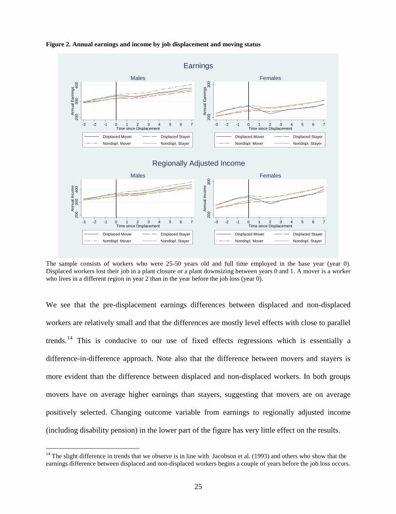
Figure 2. Annual earnings and income by job displacement and moving status

The sample consists of workers who were 25-50 years old and full time employed in the base year (year 0). Displaced workers lost their job in a plant closure or a plant downsizing between years 0 and 1. A mover is a worker who lives in a different region in year 2 than in the year before the job loss (year 0).

We see that the pre-displacement earnings differences between displaced and non-displaced

workers are relatively small and that the differences are mostly level effects with close to parallel

trends.14 This is conducive to our use of fixed effects regressions which is essentially a

difference-in-difference approach. Note also that the difference between movers and stayers is

more evident than the difference between displaced and non-displaced workers. In both groups

movers have on average higher earnings than stayers, suggesting that movers are on average

positively selected. Changing outcome variable from earnings to regionally adjusted income

(including disability pension) in the lower part of the figure has very little effect on the results.

14 The slight difference in trends that we observe is in line with Jacobson et al. (1993) and others who show that the earnings difference between displaced and non-displaced workers begins a couple of years before the job loss occurs.

200

300

400

Annu

al E

arni

ngs

-3 -2 -1 0 1 2 3 4 5 6 7Time since Displacement

Displaced Mover Displaced Stayer

Nondispl. Mover Nondispl. Stayer

Males

200

300

Annu

al E

arni

ngs

-3 -2 -1 0 1 2 3 4 5 6 7Time since Displacement

Displaced Mover Displaced Stayer

Nondispl. Mover Nondispl. Stayer

Females

Earnings20

030

040

0An

nual

Inco

me

-3 -2 -1 0 1 2 3 4 5 6 7Time since Displacement

Displaced Mover Displaced Stayer

Nondispl. Mover Nondispl. Stayer

Males

200

300

Annu

al In

com

e

-3 -2 -1 0 1 2 3 4 5 6 7Time since Displacement

Displaced Mover Displaced Stayer

Nondispl. Mover Nondispl. Stayer

Females

Regionally Adjusted Income

26

The graphs in Figure 2 are consistent with job-loss being an exogenous shock to the displaced

workers as job displacement opens up a significant earnings gap between displaced and non-

displaced workers. This is in line with the previous literature. More interesting is the finding that

the drop in earnings after job loss seems to be higher for displaced movers than for displaced

stayers. In the next section we look into this in more detail by conditioning on observable

characteristics and comparing OLS and fixed effect estimates.

The effect of job displacement on earnings and income by moving status

Table 4 gives the results of estimating equation (3) for men and women separately, with and without

individual specific fixed effects. Note that workers are included in the sample also in years when

they have zero annual earnings. This implies that we capture the joint effect of changes in

employment and wage rates.

Table 4. Effect of job displacement on earnings by moving status

Earnings Males Females OLS FE OLS FE Displaced*stay_3 5.480 0.343 (0.453)** (0.403) Displaced*stay_2 5.026 -0.453 0.523 0.237 (0.686)** (0.580) (0.428) (0.223) Displaced*stay_1 4.026 -1.454 -0.524 -0.752 (0.680)** (0.562)** (0.443) (0.277)** Displaced*stay_0 2.081 -3.402 -1.671 -1.839 (0.773)** (0.677)** (0.489)** (0.356)** Displaced*stay1 -3.375 -8.767 -3.753 -3.836 (0.738)** (0.686)** (0.558)** (0.461)** Displaced*stay2 -8.647 -14.043 -8.842 -8.818 (2.614)** (2.547)** (0.598)** (0.529)** Displaced*stay3 -7.060 -12.447 -10.001 -9.961 (2.167)** (2.094)** (0.643)** (0.576)** Displaced*stay4 -6.268 -11.668 -9.283 -9.176 (2.320)** (2.249)** (0.718)** (0.654)** Displaced*stay5 -5.464 -10.883 -9.728 -9.596 (2.027)** (1.939)** (0.709)** (0.654)** Displaced*stay6 -4.366 -9.907 -9.313 -9.128

27

(1.629)** (1.512)** (0.758)** (0.706)** Displaced*stay7 -6.164 -11.740 -9.008 -8.761 (1.174)** (1.103)** (0.792)** (0.740)** Displaced*move_3 16.413 8.659 (2.797)** (1.978)** Displaced*move_2 18.133 0.812 9.866 1.817 (2.985)** (2.139) (2.027)** (1.092) Displaced*move_1 18.000 -0.208 9.946 2.490 (3.062)** (2.326) (2.202)** (1.645) Displaced*move_0 18.594 -0.481 7.600 0.725 (2.972)** (2.438) (2.690)** (2.347) Displaced*move1 8.174 -11.724 -6.932 -12.917 (3.336)* (3.004)** (3.064)* (2.793)** Displaced*move2 -5.537 -26.520 -23.111 -28.845 (3.348) (3.147)** (3.196)** (3.173)** Displaced*move3 -2.617 -24.112 -20.065 -25.018 (3.559) (3.253)** (3.842)** (3.690)** Displaced*move4 0.929 -21.170 -19.864 -24.262 (4.038) (3.443)** (3.898)** (3.759)** Displaced*move5 -3.267 -25.622 -21.142 -25.025 (3.709) (3.553)** (4.283)** (4.120)** Displaced*move6 2.640 -20.801 -23.120 -26.590 (4.509) (4.276)** (4.306)** (4.103)** Displaced*move7 -1.035 -25.002 -20.213 -23.055 (4.350) (4.147)** (4.630)** (4.439)** Observations 7008359 7008359 2811072 2811072 R-squared 0.08 0.02 0.24 0.07 Number of groups (id x base year) 641573 256978 The sample consists of workers who were 25-50 years old and full time employed in base year 0. Displaced workers lost their job in a plant closure or plant downsizing between years 0 and 1. A mover is a worker who lives in a different region in year 2 after displacement than in the year before displacement (year 0). Annual earnings are total annual labor income and benefits such as parental and unemployment benefits. All models include base-year specific time dummies and age and age squared in interaction with base year education level and base year urban status. The OLS model also includes additional pre-displacement controls: Dummies for educational categories, marital status, tenure, cohabiting spouse, school age children, under school age children, parent in the region, spouse’s parent in the region, sibling in the region, both parent and sibling in region, younger siblings, at school in b-4, at school in b-5, regional dummies, and industry dummies. The coefficients in the 2nd and 4th columns are graphed in Figure 3. Since the FE model includes fixed effects for each individual in a given base year sample, we cannot estimate the effect for the first time period b-3. This period is thus used as base-level in the FE-regressions.

The results indicate that job loss has a long-lasting negative effect on earnings, and that the effect

is larger for movers than for stayers. We return to this below. For both men and women, there is a

clear positive pre-displacement difference in earnings between displaced stayers and movers and

the non-displaced comparison group. The pre-displacement difference is especially large for

displaced male movers. Consequently, the FE results indicate a larger negative post displacement

earnings effect for movers than do the OLS results. This implies that there is on average positive

28

selection on unobservable characteristics for movers.15 Despite this, the causal effect of moving

seems to be negative. The results are similar when we use regionally adjusted total income, i.e.

annual earnings and disability benefits, as dependent variable. These results are reported in

Appendix Table A2.

The estimated negative earnings effect is visualized in Figure 3, which plots the FE point

estimates and confidence intervals of the job displacement dummies in Table 4 separately for

movers and stayers. We observe that before the displacement incident there was no significant

difference in earnings growth between these groups. After displacement, however, earnings drop

for both groups, and significantly more so for movers than for stayers. The average annual

earnings decrease for displaced male movers in the second post displacement year is 26,500

NOK (about 4,100 US dollars). This corresponds to -7.5% when compared against counterfactual

earnings of displaced movers in the period.16 For displaced male stayers the average decrease in

the second post displacement year is -14,000 NOK, corresponding to -4.2%. We can also see that

the negative effect of job displacement is very long lasting.17

15 Appendix Table A1 shows that to some degree the selection on observables is also positive. 16 Following Davis and von Wachter (2011) the counterfactual earnings in the absence of job displacement are constructed by adding the absolute value of the estimated earnings loss to the mean earnings of the group in the period. 17 To ensure comparability of our treatment and comparison groups we have as a robustness check also estimated the FE-model using a sample that was trimmed to be similar on the basis of pre-displacement characteristics. We did this by first estimating separately the propensity of being either a displaced mover or a displaced stayer. In these regressions we used a full set of year and base year interactions, regional dummies and all pre-displacement control variables reported in Appendix Table A2. Then we trimmed the comparison group sample using these estimated propensity scores. We either used the scores as weight or dropped observations for which the estimated propensity score was higher than 0.01 (as suggested in Crump et al., 2009). The regression results we obtained when following this procedure were similar to those discussed above. The difference between movers and stayers diminished a little, and the standard errors increased.

29

Figure 3. Effects of job displacement on earnings and regionally adjusted income by moving status

The figure displays FE-coefficients and confidence intervals from Table 4, columns (2) and (4), and from a similar set of regressions with regionally adjusted income as dependent variable. The latter income measure also includes disability pension and is deflated with regional CPIs to capture differences in living expenses between regions.

For women, the difference in the earnings loss between stayers and movers is even more

pronounced. In the second post displacement year, the earnings drop for displaced female movers

is on average -28,800 NOK (about 4,500 US dollars). Since average female earnings are lower

than male average earnings, this corresponds to -12.0% of counterfactual earnings for displaced

female movers in the period. For displaced female workers who stay in the pre-displacement

region the estimated loss is only -8,800 NOK, corresponding to -3.9%.

The difference between movers and stayers may partly reflect the fact that some workers move to

regions with lower living expenses. In order to take this into account we have also run the same

regressions as in Table 4 with the regionally adjusted income measure (including disability

-40

-30

-20

-10

010

Annu

al E

arni

ngs,

100

0 N

OK

-2 -1 0 1 2 3 4 5 6 7Time Since Displacement

Stayers CI Movers CI

Stayers Movers

Males

-40

-30

-20

-10

010

Annu

al E

arni

ngs,

100

0 N

OK

-2 -1 0 1 2 3 4 5 6 7Time Since Displacement

Stayers CI Movers CI

Stayers Movers

Females

Earnings

-40

-30

-20

-10

010

Annu

al In

com

e, 1

000

NO

K

-2 -1 0 1 2 3 4 5 6 7Time Since Displacement

Stayers CI Movers CI

Stayers Movers

Males

-40

-30

-20

-10

010

Annu

al In

com

e, 1

000

NO

K-2 -1 0 1 2 3 4 5 6 7

Time Since Displacement

Stayers CI Movers CI

Stayers Movers

Females

Regionally Adjusted Income

30

pension) as dependent variable. The results are reported in Appendix Table A2, and graphed in

the lower panel of Figure 3. Again, we find that movers have larger income losses after job

displacement than stayers. The short-term magnitude is about the same as for earnings, but the

difference between movers and stayers diminishes somewhat more over time. The drop in annual

income in the second post displacement year for male movers is -26,900 NOK (6.9%) and for

male stayers -15,300 NOK (4.1%). For female workers, the effect for movers is -27,900 NOK (-

10.6%) and for stayers -9,500 NOK (-3.8%).

Since Mincer (1978) it has been well established that it is the net family gain rather than the net

personal gain that motivates the migration of households. The possible net loss of a tied mover

must be smaller than the net gain of his or her spouse to result in a net family gain. In order to

take into account the fact that many of the displaced movers may be so-called tied movers, we

also estimate the effect of displacement and mobility on total family income for a sample of

workers that had a spouse in the base year. Total family income is the sum of a worker’s own

annual real income and the annual real income of the spouse. The regression results with total

family income as dependent variable are presented in the lower panel of Figure 4. For

comparison, own income-results are presented in the upper panel.

For displaced males with a spouse in the base year, job loss has a negative effect on both own

income and family income. This is to be expected. As before, we also see that movers have larger

losses than stayers in the years immediately following job loss. The family income loss in year 2

for displaced male movers that have a spouse in the base year is 36,900 NOK (-7.4%) and for

similar displaced male stayers it is 13,500 NOK (-2.9%). However, while the difference between

31

movers and stayers in own income is relatively constant over time, the difference in family

income seems to fade away and is statistically insignificant by year 7.

Figure 4. Effect of job displacement on own and family income for base year couples

The sample is restricted to workers that were married or had a cohabiting spouse in year 0. The dependent variable is own annual taxable real income in the upper panel, and total family income in the lower panel. Family income is income including disability pension for both the worker and the spouse (married or cohabiting partner). The regressions include individual fixed effects. See the subtext to Table 4 for further details about the specification.

For displaced female movers that have a spouse in the base year, the drop in year 2 family

income is 26,500 NOK (-6.1%) and for similar female stayers it is 11,800 NOK (-2.6%). Even

though these short-term losses are close to the estimates for males, there is an important contrast

between female and male workers. For displaced female workers that have a spouse in the base

year, it is quite evident that the difference between movers and stayers in family income is

temporary, and the estimated difference is not statistically significant at any point in time. Most

-60

-40

-20

020

Annu

al In

com

e, 1

000

NO

K

-2 -1 0 1 2 3 4 5 6 7Time Since Displacement

Stayers CI Movers CI

Stayers Movers

Males

-60

-40

-20

020

Annu

al In

com

e, 1

000

NO

K

-2 -1 0 1 2 3 4 5 6 7Time Since Displacement

Stayers CI Movers CI

Stayers Movers

Females

Own Income

-60

-40

-20

020

40Fa

mily

Inco

me,

100

0 N

OK

-2 -1 0 1 2 3 4 5 6 7Time Since Displacement

Stayers CI Movers CI

Stayers Movers

Males

-60

-40

-20

020

40Fa

mily

Inco

me,

100

0 N

OK

-2 -1 0 1 2 3 4 5 6 7Time Since Displacement

Stayers CI Movers CI

Stayers Movers

Females

Family Income

32

likely, this is because female displaced workers to a larger extent than male displaced workers are

tied movers.

To what extent does the earnings loss depend on where you move to?

In order to further understand why there seems to be a negative causal effect of mobility on own

income (i.e. conditional on worker fixed effects), we cut the data by the characteristics of the

locations that the displaced workers move to. More specifically, we distinguish between whether

workers move to an urban or a rural location, and whether they move to a region where they or

their spouse have parents. We acknowledge that this analysis is descriptive in nature, since the

decision to move to a certain destination is endogenous.

Figure 5 reports the results of fixed effects regressions where we estimate how the income loss

for displaced movers and stayers varies between urban and rural regions determined by the

workers’ location in post displacement year 2. About 60% of the displaced stayers live in an

urban region in year b+2, and about 50% of the displaced movers live in an urban region in year

b+2. The results show that displaced workers who move to urban regions do not suffer any

significant post-displacement earnings losses at all. The negative effect of job displacement for

movers is entirely driven by individuals who move to rural locations. These workers suffer severe

and long-lasting income losses. Stayers in urban and rural locations also suffer some income

losses after job displacement, but the drop is much smaller than the drop for workers who move

to rural regions. Note also that there is no significant difference between the income losses for

displaced workers who stay in an urban location and those who move to urban locations.

33

Figure 5. Effect of job displacement by mobility and urban status

A mover is a worker who lives in a different region in year 2 after displacement than in the year before displacement (year 0). The dependent variable is real annual income. Urban region means that the worker lives in one of the ten biggest commuting areas in Norway in year 2. The other regions are classified as rural. The regressions include individual fixed effects. See the subtext to Table 4 for further details about the regression and sample.

In order to examine the role played by family, we also split the sample by the parents’ location in

post displacement year 2. About 65% of the displaced stayers live in the same region as their

parents or their spouse’s parents in year b+2, and about 35% of the displaced movers live in the

same region as their parents or their spouse’s parents in year b+2. We estimate the same

regressions as those graphed in Figure 5, but we let the effect of job displacement for movers and

stayers vary between workers with and without parents (or parents of the spouse) in the region in

year b+2. The results indicate that workers who move to a region where they or their spouse have

parents suffer bigger earning losses than workers who move to regions where they have no

-60

-40

-20

020

Annu

al In

com

e, 1

000

NO

K

-2 -1 0 1 2 3 4 5 6 7Time Since Displacement

Stayers CI Movers CI

Stayers Movers

Urban

-60

-40

-20

020

Annu

al In

com

e, 1

000

NO

K

-2 -1 0 1 2 3 4 5 6 7Time Since Displacement

Stayers CI Movers CI

Stayers Movers

Rural

Males

-60

-40

-20

020

Annu

al In

com

e, 1

000

NO

K

-2 -1 0 1 2 3 4 5 6 7Time Since Displacement

Stayers CI Movers CI

Stayers Movers

Urban

-60

-40

-20

020

Annu

al In

com

e, 1

000

NO

K-2 -1 0 1 2 3 4 5 6 7

Time Since Displacement

Stayers CI Movers CI

Stayers Movers

Rural

Females

34

family. It is striking that for displaced male workers there is no difference between movers and

stayers living in a region where they do not have family.

Figure 6. Effect of job displacement by mobility and family ties in the region

A mover is a worker who lives in a different region in year 2 after displacement than in the year before displacement (year 0). The dependent variable is real annual income. Family in region means that parents of the worker or the worker’s spouse live in the same region as the worker in year 2 after displacement. The regressions include individual fixed effects. See the subtext to Table 4 for further details about the regression and sample.

Selection into mobility after job loss

The negative employment shock that displaced workers experience changes the incentives to

migrate, but it is not clear what type of worker it is that reacts more easily to the shock. However,

our results so far suggest that movers on average are positively selected and that non-economic

factors matter.

-60

-40

-20

020

Annu

al In

com

e, 1

000

NO

K

-2 -1 0 1 2 3 4 5 6 7Time Since Displacement

Stayers CI Movers CI

Stayers Movers

Family

-60

-40

-20

020

Annu

al In

com

e, 1

000

NO

K

-2 -1 0 1 2 3 4 5 6 7Time Since Displacement

Stayers CI Movers CI

Stayers Movers

No Family

Males

-40

-20

020

Annu

al In

com

e, 1

000

NO

K

-2 -1 0 1 2 3 4 5 6 7Time Since Displacement

Stayers CI Movers CI

Stayers Movers

Family

-40

-20

020

Annu

al In

com

e, 1

000

NO

K

-2 -1 0 1 2 3 4 5 6 7Time Since Displacement

Stayers CI Movers CI

Stayers Movers

No Family

Females

35

In order to assess selection into mobility in more detail, we display in Figure 7 the full base year

income distribution of displaced workers by gender and moving status at b+2. We see that

movers tend to be more represented in both ends of the income distributions, and that this is

particularly evident for male movers.

Figure 7. Pre-displacement income distribution for displaced workers by moving status

Annual income in base year 0. The sample consists of workers who were 25-50 years old and full time employed in base year 0, and who were displaced from their jobs between years 0 and 1. Workers earning more than 1000 000 NOK are excluded from the figures.

Much of the income differences between movers and stayers, however, can be explained by

observable differences. Movers are younger, more educated, more likely to be single or childless,

and less likely to have family members in regions as shown in Table A1. We can control for

these factors by looking at the residuals from a wage regression where we control for the

observable background characteristics. This is done in Figure 8. We see that even though much

02.

000e

-064

.000

e-06

6.00

0e-0

6In

com

e D

ensi

ty

0 200000 400000 600000 800000 1000000x

Stayers Movers

Males

02.

000e

-06

4.00

0e-0

66.

000e

-06

8.00

0e-0

6In

com

e D

ensi

ty0 200000 400000 600000 800000 1000000

x

Stayers Movers

Females

0.2

.4.6

.81

0 200000 400000 600000 800000 1000000Base Year Income

Stayers Movers

Males

0.2

.4.6

.81

0 200000 400000 600000 800000 1000000Base Year Income

Stayers Movers

Females

36

of the differences in income between movers and stayers are explained by differences in

observables, movers are still more represented in both ends of the distribution.

Figure 8. Pre-displacement residual income distribution for displaced workers by moving status

Annual income residuals in base year 0. The income residuals are obtained by regressing base year income on the following control variables: Dummies for educational categories, marital status, tenure, cohabiting spouse, school age children, under school age children, parent in the region, spouse’s parent in the region, sibling in the region, both parent and sibling in region, younger siblings, at school in b-4, at school in b-5, regional dummies, and industry dummies. The sample consists of workers who were 25-50 years old and full time employed in base year 0, and who were displaced from their jobs between years 0 and 1. Workers earning more than 1000 000 NOK are excluded from the figures.

6 Concluding remarks It is well-established that there are large and persistent differences in unemployment rates and

economic activity across different locations. We also know that individuals that lose their jobs for

exogenous reasons suffer long-lasting and permanent earnings losses. Much less is known about

the reasons for these losses and why individuals with severe losses do not move to locations with

02.

000e

-064

.000

e-06

6.00

0e-0

6R

esid

ual I

ncom

e D

ensi

ty

-500000 0 500000 1000000x

Stayers Movers

Males

02.

000e

-06

4.00

0e-0

66.

000e

-06

8.00

0e-0

6R

esid

ual I

ncom

e D

ensi

ty

-500000 0 500000 1000000x

Stayers Movers

Females

0.2

.4.6

.81

-500000 0 500000 1000000Income Residual

Stayers Movers

Males0

.2.4

.6.8

1

-500000 0 500000 1000000Income Residual

Stayers Movers

Females

37

better employment opportunities. We have analyzed the geographic mobility of workers after

permanent job loss, and investigated factors that influence workers’ migration decision. Our rich

Norwegian register data include information about the workers’ characteristics, location and

employment histories, as well as information about spouses, children, parents and siblings.

Our results show that family ties are very important for workers’ mobility decision. Workers are

less likely to move away from regions where their parents or siblings live, and some move back

home after a job loss. We also provide evidence of how earnings losses after job displacement are

related to migration. Our findings suggest that workers who move to a new region after job loss

suffer larger income losses than stayers, although the difference between movers and stayers in

total family income is smaller and tends to fade away over time. We also find that the difference

in individual earnings between displaced movers and stayers is driven entirely by workers who

move to rural regions or to regions where they have family members. All in all, our study

provides new evidence on the importance of non-economic factors in explaining migration

decisions and income losses following job displacement.

References

Abramitzky, Ran, Leah Platt Boustan and Katherine Eriksson, (2012). Europe’s Tired, Poor,

Huddled Masses: Self-Selection and Economic Outcomes in the Age of Mass Migration,

American Economic Review, 102(5), 1832–1856.

Alesina, Alberto F., Yann Algan, Pierre Cahuc and Paola Giuliano (2010). Family Values and the

Regulation of Labor, NBER Working Papers 15747. Forthcoming in Journal of the

European Economic Association.

38

Autor, David H., David Dorn and Gordon H. Hanson (2013). The China Syndrome: Local Labor

Market Effects of Import Competition in the United States, American Economic Review,

103(6), 2121–2168.

Balsvik, Ragnhild, Sissel Jensen, and Kjell G. Salvanes (2014). Made in China, Sold in Norway:

Local Labor Market Effects of an Import Shock, IZA Discussion Papers 8324.

Forthcoming in Journal of Public Economics.

Bhuller, Manudeep S. (2009). Inndeling av Norge i arbeidsmarkedsregioner, Notater 2009/24,

Statistics Norway.

Blanchard, Olivier J. and Lawrence F. Katz (1992). Regional Evolutions, Brookings Papers on

Economic Activity, Economic Studies Program, 23(1), 1–76.

Boman, Anders (2011). Does migration pay? Earnings effects of geographic mobility following

job displacement, Journal of Population Economics, 24(4), 1369–1384.

Borjas, George J, (1987). Self-Selection and the Earnings of Immigrants, American Economic

Review, 77(4), 531–553.

Borjas, George J. (1991). Immigration and Self-selection. In J. M. Abowd and R. B. Freeman

(Eds.): Immigration, Trade and the Labor Market, pp. 29–76. University of Chicago

Press.

Press.Borjas, George J., Stephen G. Bronars, and Stephen J. Trejo (1992). Self-selection and

internal migration in the United States, Journal of Urban Economics, 32(2), 159-185.

Bütikofer, Aline, Darina Polovkova and Kjell G. Salvanes (2014), Cities and Wages: Urban

Wage Premium and Migrant Selection, mimeo, Norwegian School of Economics

Couch, Kenneth A, and Dana W. Placzek (2010). Earnings Losses of Displaced Workers

Revisited, American Economic Review, 100(1), 572–589.

Crump, Richard K., V. Joseph Hotz, Guido W. Imbens and Oscar A. Mitnik, (2009). Dealing

with limited overlap in estimation of average treatment effects, Biometrika, 96(1), 187–

199.

39

Davis, Steven J. and Till von Wachter (2011). Recessions and the Costs of Job Loss, Brooking

Papers on Economic Activity, 1–72.

Eliason, Marcus and Donald Storrie (2006). Lasting or Latent Scars? Swedish Evidence on the

Long-Term Effects of Job Displacement, Journal of Labor Economics, 24(4), 831–856.

Glaeser, Edward L and David C. Mare (2001). Cities and Skills, Journal of Labor Economics,

19(2), 316–342.

Glaser, Karen F. and Cecilia Tomassini (2000) Proximity to children: a comparison of Britain

and Italy, The Gerontologist, 40(6), 729–737.

Greenwood, Michael J. (1997), The Internal Migration in Developed Countries, Ch. 12 in M. R.

Rosenzweig and O. Stark (eds.), Handbook of Population and Family Economics.

Volume 1, Part B, pp. 647–720.

Huttunen, Kristiina, Jarle Møen and Kjell G. Salvanes, (2011). How Destructive is Creative

Destruction? Effects of Job Loss on Job Mobility, Withdrawal and Income, Journal of the

European Economic Association, 9(5), 840–870.

Jacobson, Louis S., Robert J. LaLonde and Daniel G. Sullivan (1993): Earnings Losses of

Displaced Workers, American Economic Review, 83(4), 685–709.

Konrad, Kai A., Harald Künemund, Kjell Erik Lommerud and Julio R. Robledo (2002).

Geography of the Family, American Economic Review, 92(4), 981–998.

Kramarz, Francis and Oskar Nordström Skans (2011). When Strong Ties are Strong: Networks

and Youth Labor Market Entry, Center for Labor Studies Working Paper Series 2011:18,

Uppsala University. Forthcoming in Review of Economic studies.

Lin, Ge and Peter A. Rogerson (1995). Elderly Parents and the Geographic Availability of Their

Adult Children, Research on Aging, 17(3), 303–331

Machin, Stephen, Kjell G. Salvanes and Panu Pelkonen (2012). Education And Mobility, Journal

of the European Economic Association, 10(2), 417–450.

40

Mincer, Jacob (1978). Family Migration Decisions, Journal of Political Economy, 86(5), 749–

773.

Rainer, Helmut and Thomas Siedler (2009). O Brother, Where Art Thou? The Effects of Having

a Sibling on Geographic Mobility and Labour Market Outcomes, Economica, 76(303),

528–556.

Rees, Phillip and Marek Kupiszewski (1999). Internal Migration and Regional Population

Dynamics in Europe: A Synthesis, Population studies No. 32, Council of Europe,

Strasbourg.

Rees Phillip, Lars Østby, Helen Durham, Marek Kupiszewski (1999). Internal Migration and

Regional Population Dynamics in Europe: Norway Case Study, Reports 99/19, Statistics

Norway.

Rege, Mari, Kjetil Telle and Mark Votruba, (2009). The Effect of Plant Downsizing on

Disability Pension Utilization, Journal of the European Economic Association, 7(4), 754–

785.

Roy, Andrew D. (1951). Some Thoughts on the Distribution of Earnings, Oxford Economic

Papers (New series), 3(2), 135–146.

Schmieder, Johannes F., Till von Wachter and Stefan Bender (2009). The Long-Term Impact of

Job Displacement in Germany During the 1982 Recession on Earnings, Income, and

Employment, Discussion Papers 0910-07, Department of Economics, Columbia

University.

41

Appendix Table A1. Sample means of selected pre-displacement characteristics Males Females Displaced

Movers Displaced

Stayers Non-

displaced Movers

Non-displaced Stayers

Displaced Movers

Displaced Stayers

Non-displaced Movers

Non-displaced Stayers

Age 35.14** 38.11 34.71** 38.33 33.45** 37.69 33.43** 38.12 (0.14) (0.03) (0.06) (0.01) (0.21) (0.04) (0.10) (0.02) Secondary 0.56** 0.63 0.54** 0.63 0.60** 0.65 0.57** 0.64 education (0.01) (0.00) (0.00) (0.00) (0.02) (0.00) (0.01) (0.00) Tertiary 0.34** 0.21 0.36** 0.21 0.30** 0.189 0.34** 0.19 education (0.01) (0.00) (0.00) (0.00) (0.01) (0.00) (0.01) (0.00) Tenure 4.65** 6.83 4.72** 7.35 4.62** 6.33 4.69** 6.76 (0.08) (0.02) (0.04) (0.01) (0.12) (0.03) (0.06) (0.01) Cohabiting 0.54** 0.73 0.56** 0.74 0.40** 0.67 0.45** 0.70 or married (0.01) (0.00) (0.00) (0.00) (0.01) (0.00) 0.01 (0.00) Years in 3.94** 4.85 3.85** 4.85 3.97** 4.85 3.92** 4.86 region (0.03) (0.00) (0.02) (0.00) (0.05) (0.00) (0.02) (0.00) No. of school 0.29** 0.44 0.27** 0.44 0.16** 0.31 0.15** 0.32 age children (0.01) (0.00) (0.00) (0.00) (0.01) (0.00) (0.01) (0.00) No. of ch. 0.27** 0.20 0.29** 0.20 0.06 0.06 0.06 0.06 under 7 (0.01) (0.00) (0.00) (0.00) (0.01) (0.00) (0.00) (0.00) Parent in 0.42** 0.69 0.43** 0.69 0.39** 0.60 0.40** 0.60 region (0.01) (0.00) (0.00) (0.00) (0.02) (0.00) (0.01) (0.00) Sibling in 0.52** 0.74 0.52** 0.75 0.46** 0.67 0.49** 0.67 region (0.01) (0.00) (0.00) (0.00) (0.02) (0.00) (0.01) (0.00) Parent and 0.36** 0.63 0.37** 0.63 0.33** 0.54 0.36** 0.63 sibl. in reg. (0.01) (0.00) (0.00) (0.00) (0.01) (0.00) 0.01 (0.00) Younger 0.51** 0.47 0.53** 0.47 0.54** 0.44 0.55** 0.44 siblings (0.01) (0.00) (0.00) (0.00) (0.02) (0.00) (0.01) (0.00) Plant size 234 248 292** 260 206 201 279** 248 (no. of w.) (7.60) (1.40) (4.85) (0.61) (10.58) (1.99) (7.67) (1.02) Earnings b-3 298467* 292242 289263 289130 212292** 202482 212917 203910 (3164) (474) (1229) (174) (2445) (439) (1119) (170) Earnings b-4 271697** 279853 265222** 277931 192053 190924.1 194377 193541 (2767) (526) (1304) (166) (2607) (443) (1203) (169) Earnings b-5 249488** 266451 241569** 266338 174012 178176 174749** 182123 (2853) (518) (1349) (164) (2751) (462) (1296) (168) Employment 10.08** 11.01 10.04** 11.13 9.38** 9.80 9.54** 9.89 months b-4 (0.09) (0.01) (0.04) (0.00) (0.14) (0.02) (0.06) (0.01) Employment 9.21** 10.53 9.13** 10.70 8.65** 9.18 8.57** 9.30 months b-5 (0.10) (0.01) (0.05) (0.00) (0.16) (0.03) (0.07) (0.01) At school b-4 0.05 0.05 0.06 0.06 0.06 0.05 0.06 0.05 (0.00) (0.00) (0.00) (0.00) (0.01) (0.00) (0.00) (0.00) At school b-5 0.05 0.05 0.05 0.05 0.05 0.05 0.05 0.05 (0.00) (0.00) (0.00) (0.00) (0.01) (0.00) (0.00) (0.00) Observations 2384 77297 10989 550903 1016 29295 4736 221931 The sample consists of workers who were 25-50 years old and full time employed in the base year. Displaced workers lost their job in a plant closure or downsizing between year 0 and year 1. When the mean for movers is significantly different from stayers, it is marked with stars. * 5% level of significance. ** 1% level of significance.

42

Table A2 Effect of job displacement on regionally adjusted income by moving status Earnings Males Females OLS FE OLS FE Displaced*Stay_3 5.758 0.258 (0.481)** (0.429) Displaced*Stay_2 5.245 -0.494 0.368 0.188 (0.733)** (0.628) (0.455) (0.238) Displaced*Stay_1 4.066 -1.656 -0.754 -0.855 (0.719)** (0.604)** (0.472) (0.298)** Displaced*Stay_0 1.835 -3.872 -2.121 -2.142 (0.814)* (0.721)** (0.521)** (0.382)** Displaced*Stay1 -4.032 -9.631 -4.337 -4.258 (0.784)** (0.735)** (0.593)** (0.493)** Displaced*Stay2 -9.730 -15.314 -9.738 -9.524 (2.863)** (2.791)** (0.634)** (0.561)** Displaced*Stay3 -7.675 -13.227 -10.700 -10.449 (2.382)** (2.304)** (0.678)** (0.607)** Displaced*Stay4 -6.455 -12.001 -9.708 -9.370 (2.532)* (2.455)** (0.754)** (0.684)** Displaced*Stay5 -5.584 -11.143 -10.007 -9.615 (2.198)* (2.105)** (0.739)** (0.678)** Displaced*Stay6 -4.210 -9.866 -9.414 -8.948 (1.739)* (1.618)** (0.784)** (0.727)** Displaced*Stay7 -6.209 -11.875 -9.109 -8.557 (1.237)** (1.166)** (0.816)** (0.757)** Displaced*Move_3 17.226 9.169 (2.958)** (2.150)** Displaced*Move_2 19.136 0.914 11.030 2.520 (3.150)** (2.221) (2.221)** (1.226)* Displaced*Move_1 19.206 0.008 11.231 3.366 (3.236)** (2.432) (2.405)** (1.827) Displaced*Move_0 19.992 -0.161 9.246 2.012 (3.228)** (2.632) (2.986)** (2.624) Displaced*Move1 9.535 -11.541 -5.656 -11.923 (3.631)** (3.253)** (3.310) (3.026)** Displaced*Move2 -4.697 -26.933 -21.922 -27.906 (3.591) (3.335)** (3.382)** (3.350)** Displaced*Move3 -1.083 -23.894 -19.037 -24.221 (3.847) (3.462)** (4.044)** (3.880)** Displaced*Move4 3.086 -20.410 -18.710 -23.290 (4.249) (3.626)** (4.088)** (3.935)** Displaced*Move5 -1.287 -25.130 -19.757 -23.763 (3.951) (3.747)** (4.484)** (4.298)** Displaced*Move6 5.880 -19.166 -21.511 -25.060 (4.783) (4.504)** (4.515)** (4.282)** Displaced*Move7 2.182 -23.516 -17.830 -20.700 (4.686) (4.442)** (4.865)** (4.633)** Observations 7008355 7008355 2811067 2811067 R-squared 0.08 0.02 0.22 0.09 Number of groups (id x base-year) 641573 256978 The dependent variable is regionally adjusted annual income. The 2nd and 4th columns are graphed in the lower panel of Figure 3. See the subtext to Table 4 and Figure 3 for information on the sample, the specifications and the variables.

43

Table A3 Effect of job displacement on family income by moving status Earnings Males Females OLS FE OLS FE Displaced*Stay_3 5.181 -0.689 (0.534)** (0.882) Displaced*Stay_2 3.996 -1.191 -1.150 -0.506 (0.744)** (0.618) (0.961) (0.676) Displaced*Stay_1 2.694 -2.502 -3.770 -3.174 (0.744)** (0.620)** (1.041)** (0.881)** Displaced*Stay_0 1.011 -4.196 -3.803 -3.260 (0.831) (0.738)** (1.112)** (1.023)** Displaced*Stay1 -4.167 -9.293 -7.756 -7.023 (0.803)** (0.756)** (1.215)** (1.177)** Displaced*Stay2 -9.107 -14.279 -12.336 -11.668 (2.634)** (2.573)** (1.381)** (1.416)** Displaced*Stay3 -7.520 -12.691 -13.857 -13.291 (2.189)** (2.125)** (1.448)** (1.502)** Displaced*Stay4 -7.315 -12.512 -11.806 -11.320 (2.339)** (2.277)** (1.432)** (1.509)** Displaced*Stay5 -6.084 -11.335 -8.459 -8.142 (2.042)** (1.968)** (1.375)** (1.484)** Displaced*Stay6 -4.399 -9.730 -5.542 -5.349 (1.641)** (1.546)** (1.270)** (1.407)** Displaced*Stay7 -5.614 -10.997 -4.820 -4.657 (1.186)** (1.147)** (1.276)** (1.435)** Displaced*Move_3 17.383 15.349 (3.255)** (4.168)** Displaced*Move_2 10.908 -7.733 5.190 -11.002 (3.364)** (2.338)** (4.323) (2.788)** Displaced*Move_1 6.707 -13.164 -0.442 -17.451 (3.409)* (2.616)** (4.417) (3.569)** Displaced*Move_0 7.031 -14.038 -7.010 -24.813 (3.494)* (2.923)** (4.826) (4.501)** Displaced*Move1 -5.210 -27.368 -28.596 -46.654 (3.675) (3.446)** (4.940)** (4.825)** Displaced*Move2 -15.049 -38.630 -34.310 -53.657 (3.723)** (3.657)** (5.093)** (5.913)** Displaced*Move3 -7.222 -31.538 -29.125 -48.949 (3.980) (3.859)** (5.802)** (6.330)** Displaced*Move4 0.245 -25.080 -20.919 -41.495 (4.424) (3.992)** (6.053)** (6.494)** Displaced*Move5 0.962 -24.726 -1.605 -22.838 (4.056) (3.999)** (6.133) (6.587)** Displaced*Move6 12.371 -14.460 11.681 -10.144 (4.713)** (4.621)** (5.998) (6.554) Displaced*Move7 10.545 -17.156 24.793 2.494 (4.500)* (4.454)** (6.109)** (6.584) Observations 7008359 7008359 2811072 2811072 R-squared 0.13 0.04 0.29 0.20 Number of groups (id x base-year) 641573 256978 The dependent variable is the annual family income. The 2nd and 4th columns are graphed in the upper panel of Figure 4. See text under Table 4 and Figure 4 for more information about the sample, the specifications and the variables.

44

Table A4. Effect of job displacement on family income by moving status for base year couples Earnings Males Females OLS FE OLS FE Displaced*Stay_3 4.684 -1.913 (0.681)** (1.182) Displaced*Stay_2 3.308 -1.393 -2.017 -0.119 (0.955)** (0.811) (1.336) (0.890) Displaced*Stay_1 2.039 -2.679 -4.920 -3.040 (0.970)* (0.818)** (1.464)** (1.197)* Displaced*Stay_0 0.950 -3.788 -4.517 -2.656 (1.096) (0.976)** (1.568)** (1.393) Displaced*Stay1 -3.999 -8.656 -8.014 -5.835 (1.044)** (0.985)** (1.711)** (1.583)** Displaced*Stay2 -8.879 -13.553 -13.873 -11.825 (3.666)* (3.570)** (1.932)** (1.914)** Displaced*Stay3 -7.500 -12.169 -13.923 -11.956 (3.011)* (2.914)** (1.950)** (1.978)** Displaced*Stay4 -7.163 -11.829 -11.308 -9.446 (3.179)* (3.082)** (1.848)** (1.924)** Displaced*Stay5 -6.876 -11.591 -9.152 -7.399 (2.777)* (2.664)** (1.722)** (1.853)** Displaced*Stay6 -3.853 -8.693 -6.622 -4.904 (2.194) (2.051)** (1.450)** (1.650)** Displaced*Stay7 -5.872 -10.790 -6.097 -4.384 (1.536)** (1.485)** (1.352)** (1.610)** Displaced*Move_3 20.022 0.129 (5.545)** (8.357) Displaced*Move_2 13.585 -7.357 -2.181 -2.512 (5.728)* (4.107) (9.299) (5.477) Displaced*Move_1 11.213 -10.623 6.151 5.634 (5.875) (4.565)* (9.804) (7.132) Displaced*Move_0 17.570 -5.134 11.841 11.154 (5.925)** (4.892) (10.610) (8.975) Displaced*Move1 9.000 -14.146 -3.235 -3.829 (6.159) (5.732)* (10.415) (9.210) Displaced*Move2 -12.321 -36.940 -25.404 -26.457 (5.957)* (5.913)** (9.487)** (10.929)* Displaced*Move3 -9.413 -34.399 -28.286 -29.529 (6.186) (6.061)** (10.404)** (11.411)** Displaced*Move4 -1.414 -27.062 -32.556 -33.808 (7.032) (6.169)** (10.085)** (11.082)** Displaced*Move5 -8.387 -34.268 -26.918 -28.017 (6.270) (6.244)** (9.338)** (10.955)* Displaced*Move6 2.867 -23.597 -14.915 -15.885 (7.620) (7.419)** (8.840) (10.901) Displaced*Move7 0.386 -26.710 -9.129 -10.218 (7.033) (6.953)** (8.664) (10.873) Observations 5071395 5071395 1897478 1897478 R-squared 0.10 0.04 0.29 0.28 Number of groups (id x base-year) 463964 173295 The dependent variable is the annual family income. The sample includes individuals who were married or cohabiting in the base year (year 0). The 2nd and 4th columns are graphed in the lower panel of Figure 4. See text under Table 4 and Figure 4 for more information about the sample, the specifications and the variables.