jjmie volume 9 number 2, april.2015 issn 1995-6665jjmie.hu.edu.jo/vol9-2/jjmie-152-14-01 proof...
TRANSCRIPT
JJMIE Volume 9 Number 2, April.2015
ISSN 1995-6665
Pages 85 - 102
Jordan Journal of Mechanical and Industrial Engineering
Hybrid DEBBO Algorithm for Tuning the Parameters of PID
Controller Applied to Vehicle Active Suspension System
Kalaivani Rajagopal * a, Lakshmi Ponnusamy
b
aResearch Scholar, DEEE, CEG, Anna University, Chennai, India
b Professor, DEEE, CEG, Anna University, Chennai, India
Received 6 Nov 2014 Accepted 9 May 2015
Abstract
This paper highlights the use of hybridizing Biogeography-Based Optimization (BBO) with Differential Evolution (DE)
algorithm for parameter tuning of Proportional Integral Derivative (PID) controller applied to Vehicle Active Suspension
System (VASS). Initially BBO, an escalating nature enthused global optimization procedure based on the study of the
ecological distribution of biological organisms, and the hybridized DEBBO algorithm which inherits the behaviours of BBO
and DE, were used to find the tuning parameters of the PID controller to improve the performance of VASS. Simulations of
passive system, active system, having PID controller with and without optimizations, were performed by considering
trapezoidal, step and a random kind of road disturbances in MATLAB/SIMULINK environment. The simulation results
point out an improvement in the results with the DEBBO algorithm which converges faster than BBO..
© 2015 Jordan Journal of Mechanical and Industrial Engineering. All rights reserved
Keywords: Vehicle Active Suspension, Biogeography-Based Optimization (BBO), Differential Evolution (DE), DEBBO, Simulation.
* Corresponding author. e-mail: [email protected].
1. Introduction
The vibration of the vehicle body can cause an
unwanted noise in the vehicle, a damage to the fittings
attached to the car and severe health problems, such as an
increase in the heart rate, spinal problems, etc. to the
passengers. Research and the development sections of
automobile industries hence promote research on vibration
control. For vehicle handling and ride comfort, the
suspension system of an automobile plays an essential
role. Vehicle handling depends on the force acting
between the road surface and the wheels. The ride comfort
is related to vehicle motion sensed by the passenger. To
improve vehicle handling and the ride comfort
performance, in preference to conventional passive system,
semi-active and active systems are being developed. The
passive system uses a static spring and a damper where as
a semi-active suspension involves the use of dampers with
variable gain. On the other hand, an active suspension
involves the passive components augmented by actuators
that supply additional forces and possesses the ability to
reduce the acceleration of sprung mass continuously as
well as to minimize the suspension deflection which
results in the improvement of the tyre grip with the road
surface [1; 2].
Research on the control strategies of Vehicle Active
Suspension System (VASS) has been concentrated on by
academicians as well since this problem is open to all. In
the past, many researchers explored several control
approaches hypothetically, simulated them with simulation
software, confirmed practically and proposed for the
control of active suspension system. The survey of optimal
control technique applications to the design of active
suspensions are listed in [3] and the emphasis is on Linear-
Quadratic (LQ) optimal control. A method for designing a
controller with a model which includes the passenger
dynamics is presented in [4]. The comparison of Linear
Matrix Inequality (LMI) based controller and optimal
Proportional Integral Derivative (PID) controller by
Abdalla et al. [5] proved the sprung mass displacement
response improvement by LMI controller with only the
suspension stroke as the feedback.
PID controller design is discussed in [5-7]. The design
of robust PI controller which is used to obtain an optimal
control is discussed in [8]. The conclusion, made by Dan
Simon [9], stimulated the idea of using Biogeography-
Based Optimization (BBO) for the optimization of PID
parameters.
In [10] the classification of the satellite image of a
particular land cover using the theory of BBO is
highlighted, concluding that with this, highly accurate land
cover features can be extracted effectively. To optimize the
element length and spacing for Yagi-Uda antenna, BBO is
used and the performance is evaluated with a method of
moment’s code NEC2 [11]. BBO algorithm, to solve both
convex and non-convex Economic Load Dispatch (ELD)
problems of thermal plants, is proposed and suggested as a
© 2015 Jordan Journal of Mechanical and Industrial Engineering. All rights reserved - Volume 9, Number 2 (ISSN 1995-6665) 86
promising alternative approach for solving the ELD
problems in practical power system [12]. Markov theory
for partial immigration based BBO [13] is used to derive a
dynamic system model. A better insight into the dynamics
of migration in actual biogeography systems is given [14];
it also helped in understanding the search mechanism of
BBO on multimodal fitness landscapes. In [15], a multi-
objective BBO algorithm is proposed to design optimal
placement of phasor measurement units, which makes the
power system network completely observable and the
simultaneous optimization of the two conflicting
objectives, such as minimization and maximization of two
different parameters, are performed. The effectiveness of
BBO over Genetic Algorithm (GA) and Particle Swam
Optimization (PSO) is highlighted [16] for an ELD
problem. The performance of BBO is tested for real-world
optimization problems with some benchmark functions
[17]. An improved accuracy yielding algorithm is
presented [18], in which the performance of BBO is
accelerated with the help of a modified mutation and clear
duplicate operators; the suitability of BBO for real time
applications is also discussed. A combination of
Differential Evolution (DE) and BBO is designed to
accelerate the convergence speed of the algorithm and of
improving the solution for the economic emission load
dispatch problem [19].
In the present paper, the preference is to optimize the
PID controller tuning parameters with hybridized DEBBO
to improve the rapidity of convergence. The likelihood of
the proposed method was verified in terms of the
computational efficiency and the outputs of the linear
VASS models which are considered for the simulation
study in comparison with BBO.
The present study is organized as follows: Quarter Car
(QC) model and Half Car (HC) model dynamics of an
active suspension system are briefly explained in section 2.
Discussion of the control scheme is presented in section 3.
In section 4, the simulation results are presented and
discussed. The final section presents the conclusion of the
study.
2. Active Suspension System
The passive suspension system has the ability to only
store and dissipate energy. Its parameters, such as spring
stiffness and damping coefficients, are fixed in order to
achieve a certain level of compromise between road
holding, load carrying and comfort. The semi active
suspension system involves a variable damper, while the
active suspension system has the ability to store, dissipate
and introduce energy to the system; it may vary its
parameters depending on the working conditions.
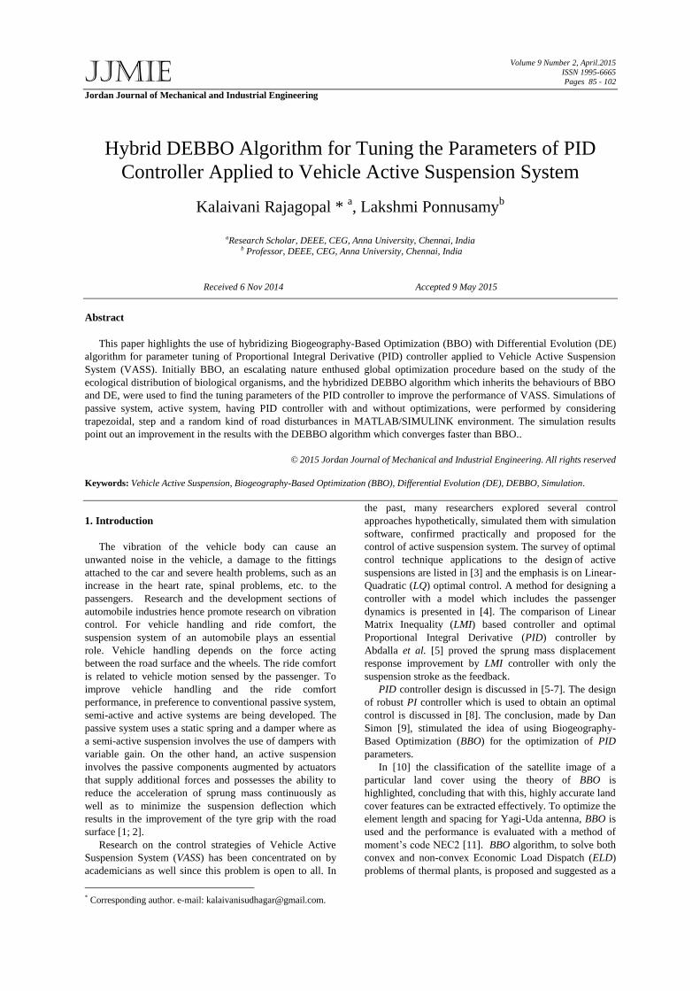
2.1. Quarter Car Model
A two-Degree of Freedom (DOF) QC model of VASS
is shown in Figure 1. It represents the automotive system
at each wheel, i.e., the motion of the axle and the vehicle
body at any one of the four wheels of the vehicle. The QC
model, used in [20], is considered because it is simple and
one can observe the basic features of the VASS such as
sprung mass displacement, body acceleration, suspension
deflection and tyre deflection. The suspension model
consists of a spring ks , a damper cs and an actuator of
active force Fa . For a passive suspension, Fa can be set
to zero. The sprung mass ms represents the QC
equivalent of the vehicle body mass. An unsprung mass
mu represents the equivalent mass due to axle and tyre.
The vertical stiffness of the tyre is represented by the
spring kt . The variables ys , yu and yt represents
the vertical displacements from static equilibrium of
sprung mass, unsprung mass and the road, respectively.
Equations of motion of the two DOF QC model of VASS
are given in (1). It is assumed that the suspension spring
stiffness and tyre stiffness are linear in their operating
ranges and that the tyre does not leave the ground. The
state space representation (2) of QC model is given below:
um
sm
tk
sk
sc
aF
sy
uy
ty
Figure 1. Quarter Car model
m y + c (y - y ) + k (y - y ) = Fu us s s s s s a (1)
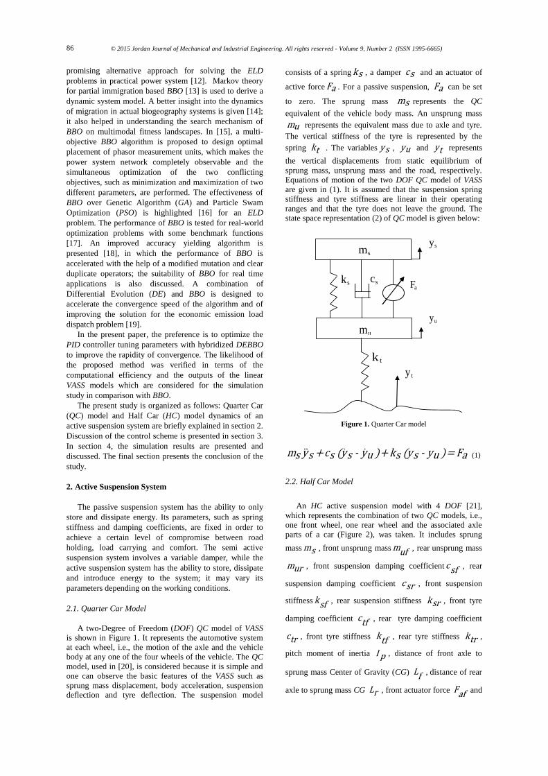
2.2. Half Car Model
An HC active suspension model with 4 DOF [21],
which represents the combination of two QC models, i.e.,
one front wheel, one rear wheel and the associated axle
parts of a car (Figure 2), was taken. It includes sprung
mass ms , front unsprung mass muf , rear unsprung mass
mur , front suspension damping coefficient csf , rear
suspension damping coefficient csr , front suspension
stiffness ksf , rear suspension stiffness ksr , front tyre
damping coefficient ctf , rear tyre damping coefficient
ctr , front tyre stiffness ktf , rear tyre stiffness ktr ,
pitch moment of inertia I p , distance of front axle to
sprung mass Center of Gravity (CG) Lf , distance of rear
axle to sprung mass CG Lr , front actuator force Faf and
© 2015 Jordan Journal of Mechanical and Industrial Engineering. All rights reserved - Volume 9, Number 2 (ISSN 1995-6665) 87
the rear actuator force Far . ,ys are the vertical
displacement and the pitch angle of the sprung mass at the
CG, ,y ysrsf are the vertical displacement of front and
rear suspensions, ,y yuruf are the unsprung mass
displacements and ,y ytrtf are the tyre displacements at
the front and rear. It is assumed that the HC model system
is linear, the tires always have contact with the road and
the forces due to moment and backlash in various joints, linkages and gear are neglected.
Figure 2. Half Car model
m y - c (y - y ) - k (y - y ) - k (y - y ) = - Fu u u u us s s s at t (2)
[-k (y - y ) - c (y - y ) - k (y - y ) - c (y - y ) - F ]ur sr ur sr sr ur sr ur artr tr tr try =urmur
(3)
[-k (y - y ) - c (y - y ) - k (y - y ) - c (y - y ) - F ]tf uf tf sf uf sf sf uf sf tf uf tf afy =uf muf
(4)
-[k (y - y ) + k (y - y ) + c (y - y ) + c (y - y ) - F - F ]sr sr ur sr sr ur arsf sf uf sf sf uf afy =sms
(5)
-L [(c (y - y ) + k (y - y )] + L [k (y - y ) + c (y - y )] - L F + L Fr sr sr ur sr sr ur r arf sf sf uf sf sf uf f afθ =Is
(6)
y = y - L θsr s r (7)
y = y + L θssf f (8)
For the passive suspension system, the control forces in
the front and rear Faf and Far are equal to 0.
3. Controller Design
3.1. PID Controller
Most of the automated industrial processes include a
PID controller which is a combination of proportional,
integral and derivative controller that can improve both the
transient and the steady state performance of the system.
The mathematical representation of the simple PID control
scheme is given by:
de
G = k e(t) + k e(t)dt + kc p i d dt (9)
where Gc is the controller output
k p proportional gain
ki integral gain
kd differential gain
© 2015 Jordan Journal of Mechanical and Industrial Engineering. All rights reserved - Volume 9, Number 2 (ISSN 1995-6665) 88
e(t) input to the controller
e(t)dt time integral of the input signal
de
dt time derivative of the input signal
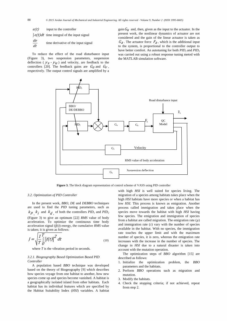
To reduce the effect of the road disturbance input
(Figure 3), two suspension parameters, suspension
deflection ( y - yus ) and velocity, are feedback to the
controllers [20]. The feedback gains are Ge and Gv ,
respectively. The output control signals are amplified by a
gainGu and, then, given as the input to the actuator. In the
present work, the nonlinear dynamics of actuator are not
considered and the gain of the linear actuator is taken as
Ga . The actuator force Fa , which is the additional input
to the system, is proportional to the controller output to
have better comfort. An autotuning for both PID1 and PID2
was carried out using a robust response tuning metod with
the MATLAB simulation software.
Figure 3. The block diagram representation of control scheme of VASS using PID controller
3.2. Optimization of PID Controller
In the present work, BBO, DE and DEBBO techniques
are used to find the PID tuning parameters, such as
k p ,ki and kd , of both the controllers PID1 and PID2
(Figure 3) to give an optimum [22] RMS value of body
acceleration. To optimize the continuous time body
acceleration signal (f(t)) energy, the cumulative RMS value
is taken; it is given as follows:
T1 2
J = f(t) dtT 0
(10)
where T is the vibration period in seconds.
3.2.1. Biogeography Based Optimization Based PID
Controller
A population based BBO technique was developed
based on the theory of Biogeography [9] which describes
how species voyage from one habitat to another, how new
species come up and species become vanished. A habitat is
a geographically isolated island from other habitats. Each
habitat has its individual features which are specified by
the Habitat Suitability Index (HSI) variables. A habitat
with high HSI is well suited for species living. The
migration of a species among habitats takes place when the
high HSI habitats have more species or when a habitat has
low HSI. This process is known as emigration. Another
process called immigration and takes place when the
species move towards the habitat with high HSI having
few species. The emigration and immigration of species
from a habitat are called migration. The emigration rate (µ)
and immigration rate (λ) vary with the number of species
available in the habitat. With no species, the immigration
rate touches the upper limit and with the maximum
number of species, it is zero, whereas the emigration rate
increases with the increase in the number of species. The
change in HSI due to a natural disaster is taken into
account with the mutation operation.
The optimization steps of BBO algorithm [15] are
described as follows:
1. Initialize the optimization problem, the BBO
parameters and the habitats.
2. Perform BBO operations such as migration and
mutation.
3. Modify the habitats.
4. Check the stopping criteria; if not achieved, repeat
from step 2.
Velocity
Suspension deflection Ge
Gv
RMS value of body acceleration
aF
QC Model
Road disturbance input
sz
BBO/
DE/DEBBO
PID1
PID2
Gu
Ga
© 2015 Jordan Journal of Mechanical and Industrial Engineering. All rights reserved - Volume 9, Number 2 (ISSN 1995-6665) 89
BBO does not involve the reproduction of a solution as
in GA. In each generation, the fitness of every solution
(habitat) is used to find the migration rates.
For the BBO based PID (BBOPID) controller [23], the
following parameters are initialized: population size, the
maximum species count (Smax), maximum emigration rate
(E), maximum immigration rate (I), maximum mutation
rate (mmax), habitat modification probability (Pmod), number
of decision variables, the number of habitats, maximum
number of generations, mutation probability, and
migration probability.
1. The individual habitat variables are random initialized.
2. Mapping of HSI to the number of species S, calculation
of the emigration rate and immigration rate using
equations 11 and 12 are performed.
dλ = I(1 - )
Smax (11)
E × dμ =
Smax (12)
where d is the number of species at the instant of time.
3. The BBO operation migration is performed based on
the definition 7 in [9] and the HSI is recomputed.
4. Then the mutation operation is performed as in
definition 8 in [9] and the HSI is recomputed. The
emigration and immigration rates of each solution are
useful in probabilistically sharing the information
between the habitats. Each solution can be modified
with the habitat modification probability Pmod to yield
good solution.
5. From step 2 the computation is repeated for the next
iteration. The loop is terminated after predefined
number of generations or after achievement of
acceptable solution.
Parameter Initialization for BBO
Modification probability = 1
Mutation probability = 0.05
Selectiveness parameter δ = 2
Max immigration rate = 1
Max emigration rate = 1
Step size used for numerical integration = 1
Lower bound and Upper bound for
immigration probability per gene = [0.01, 1]
3.2.2. Differential Evolution Based PID Controller
Technically, a simple population-based Differential
Evolution (DE) algorithm [24, 25] having a self-organizing
ability, is suitable even for non-linear systems and can be
used for a continuous function optimization for tuning of
PID controller parameters. Basic steps involved in DE
algorithm are:
1. Initialization
2. Evaluation
3. Repeat
{ Mutation
Recombination
Evaluation
Selection }
Until fitness function is minimized.
Generate the mutant vector vi,G+1 (13) for each
target vector xi,G , i=1,2,3…….N where N is the number of
parameter vectors in the population.
v = x + F.(x - x )i,G+1 r1,G r2,G r3,G
r ,r ,r 1,2,……N1 2 3
(13)
The real and constant scaling factor for differential
variation F [0,2]
The trial vector for crossover operation is
u = (u ,u ……u )i,G+1 1i,G+1 2i,G+1 Di,G+1 (14)
where
u = v if(randb(j) CR)orj = rnbr(i)ji,G+1 ji,G+1
x if(randb(j) > CR)andj rnbr(i)ji,G (15)
1,2,j D
where
CR [0,1] is the crossover constant
randb(j) [0,1] is the jth evaluation of uniform
random number
rnbr(i) 1,2,……D randomly chosen index which
ensures that ui,G+1gets at least one parameter
fromvi,G+1.
The fitness criterion is used to decide whether the trial
vector is a member of next generation. If the fitness value
of the trial vector ui,G+1 is better than that of target
vector xi,G , then, in next generation, the target vector
xi,G+1 is assigned to be ui,G+1 . Otherwise first
generation value ,i Gx is retained.
Parameter Initialization for DE
Scaling factor F = 0.5
Crossover constant CR = 0.5
3.2.3. Hybridization
The BBO algorithm, without hybridizing with any
evolutionary algorithms, does not have much diversity in
local or sub optimal solutions. In DEBBO, a hybrid
migration operator of BBO is applied along with mutation,
crossover and selection operators of DE which combines
the searching of DE with the operation of BBO effectively
to speed up the convergence property [26, 27] and to find
better quality results.
Parameters for DEBBO are initialized as in BBO and
DE.
© 2015 Jordan Journal of Mechanical and Industrial Engineering. All rights reserved - Volume 9, Number 2 (ISSN 1995-6665) 90
0 20 40 60 80 100 12050
100
150
200
250
300
350
Iteration Number
Obje
ctive
Fu
ncti
on V
alu
e (
x1
0 -3m
/s2)
BBO
DE
DEBBO
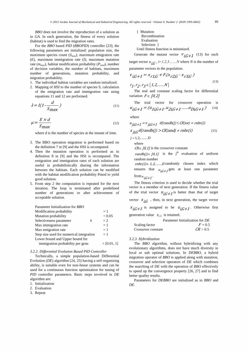
Figure 4. Statistics of search process
The optimization results were computed by averaging
20 minimization runs and the convergence characteristics
of each technique are shown in Figure 4. As the
convergence rate is fast in the case of DEBBO, the
corrective actions can be taken quickly compared to the
BBO without hybridization for a VASS. DEBBO yields sub
linear convergence. Each run yielded the global minimum
results. From the convergence plot, DEBBO is found to be
superior to the BBO algorithm.
4. Simulation
The parameters of the QC model, taken from [20], are
listed below:
Sprung mass ( ms ) : 290 kg
Unsprung mass ( mu ) : 59 kg
Damper coefficient ( cs ) : 1,000 Ns/m
Suspension stiffness ( ks ) : 16,812 N/m
Tyre stiffness ( kt ) : 190,000 N/m
The parameters of the HC model, taken from [21], are
listed below:
Sprung mass (ms) : 430 kg
Pitch moment of inertia (Ip) : 600 kgm2
Front unsprung mass (muf) : 30 kg
Rear unsprung mass (mur) : 25 kg
Front suspension damping
coefficient (csf) : 500Ns/m
Rear suspension damping
coefficient (csr) : 400Ns/m
Front tyre damping coefficient(ctf) : 24Ns/m
Rear tyre damping coefficient (ctr) : 24Ns/m
Front suspension stiffness (ksf) : 6666.67N/m
Rear suspension stiffness (ksr) : 10000N/m
Front tyre stiffness (ktf) : 152N/m
Rear tyre stiffness (ktr) : 152N/m
Distance of front axle to
sprung mass CG (Lf) : 0.871m
Distance of rear axle to
sprung mass CG (Lr) : 1.469m
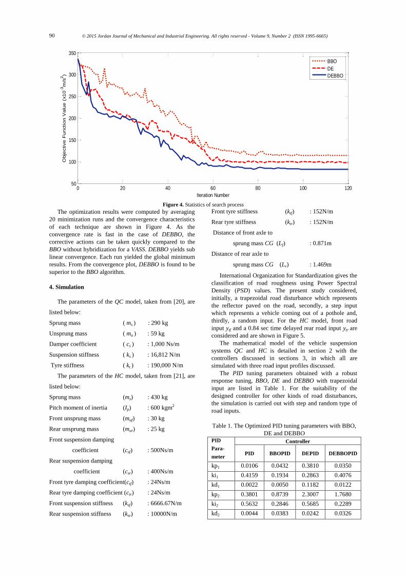
International Organization for Standardization gives the
classification of road roughness using Power Spectral
Density (PSD) values. The present study considered,
initially, a trapezoidal road disturbance which represents
the reflector paved on the road, secondly, a step input
which represents a vehicle coming out of a pothole and,
thirdly, a random input. For the HC model, front road
input ytf and a 0.84 sec time delayed rear road input ytr are
considered and are shown in Figure 5.
The mathematical model of the vehicle suspension
systems QC and HC is detailed in section 2 with the
controllers discussed in sections 3, in which all are
simulated with three road input profiles discussed.
The PID tuning parameters obtained with a robust
response tuning, BBO, DE and DEBBO with trapezoidal
input are listed in Table 1. For the suitability of the
designed controller for other kinds of road disturbances,
the simulation is carried out with step and random type of
road inputs.
Table 1. The Optimized PID tuning parameters with BBO,
DE and DEBBO PID
Para-
meter
Controller
PID BBOPID DEPID DEBBOPID
kp1 0.0106 0.0432 0.3810 0.0350
ki1 0.4159 0.1934 0.2863 0.4076
kd1 0.0022 0.0050 0.1182 0.0122
kp2 0.3801 0.8739 2.3007 1.7680
ki2 0.5632 0.2846 0.5685 0.2289
kd2 0.0044 0.0383 0.0242 0.0326
© 2015 Jordan Journal of Mechanical and Industrial Engineering. All rights reserved - Volume 9, Number 2 (ISSN 1995-6665) 91
0 0.5 1 1.5 2 2.5 3 3.5 4 4.5 50
0.005
0.01
0.015
0.02
0.025
Time (sec)
Roa
d I
nput
Am
plit
ude
(m
)
Front Road Input Rear Road Input
(a)
0 0.5 1 1.5 2 2.5 3 3.5 4 4.5 50
0.01
0.02
0.03
0.04
0.05
0.06
Time (sec)
Roa
d I
np
ut
Am
plitu
de
(m
)
Front Road Input Rear Road nput
(b)
0 1 2 3 4 5 6 7 8 9 10
-0.02
-0.015
-0.01
-0.005
0
0.005
0.01
0.015
0.02
0.025
Time (sec)
Roa
d I
np
ut
Am
plitu
de
(m
)
Front Road Input Rear Road Input
(c )
Figure 5. Road Input profile : (a) Trapezoidal Input (b) Step Input (c ) Random Input
© 2015 Jordan Journal of Mechanical and Industrial Engineering. All rights reserved - Volume 9, Number 2 (ISSN 1995-6665) 92
0 0.5 1 1.5 2 2.5 3 3.5 4 4.5 5-0.015
-0.01
-0.005
0
0.005
0.01
0.015
0.02
0.025
0.03
0.035
Time (sec)
Spru
ng M
ass D
isp
lace
me
nt
(m)
Passive
PID
BBOPID
DEPID
DEBBOPID
(a)
0 0.5 1 1.5 2 2.5 3 3.5 4 4.5 5-2
-1.5
-1
-0.5
0
0.5
1
1.5
2
Time (sec)
Bod
y A
ccele
rati
on
(m
/s2)
Passive
PID
BBOPID
DEPID
DEBBOPID
(b)
0 0.5 1 1.5 2 2.5 3 3.5 4 4.5 5-0.025
-0.02
-0.015
-0.01
-0.005
0
0.005
0.01
0.015
0.02
Time (sec)
Susp
en
sio
n D
efl
ecti
on
(m
)
Passive
PID
BBOPID
DEPID
DEBBOPID
(c)
© 2015 Jordan Journal of Mechanical and Industrial Engineering. All rights reserved - Volume 9, Number 2 (ISSN 1995-6665) 93
0 0.5 1 1.5 2 2.5 3 3.5 4 4.5 5-5
-4
-3
-2
-1
0
1
2
3
4
5x 10
-3
Time (sec)
Tyr
e D
efl
ecti
on (
m)
Passive
PID
BBOPID
DEPID
DEBBOPID
(d)
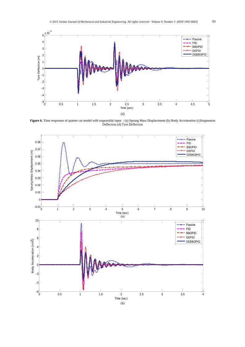
Figure 6. Time responses of quarter car model with trapezoidal input : (a) Sprung Mass Displacement (b) Body Acceleration (c)Suspension
Deflection (d) Tyre Deflection
0 1 2 3 4 5 6 7 8 9 10-0.01
0
0.01
0.02
0.03
0.04
0.05
0.06
0.07
0.08
Time (sec)
Spru
ng M
ass D
isp
lace
me
nt
(m)
Passive
PID
BBOPID
DEPID
DEBBOPID
(a)
0 0.5 1 1.5 2 2.5 3 3.5 4-6
-4
-2
0
2
4
6
8
10
Time (sec)
Bod
y A
ccele
rati
on
(m
/s2)
Passive
PID
BBOPID
DEPID
DEBBOPID
(b)
© 2015 Jordan Journal of Mechanical and Industrial Engineering. All rights reserved - Volume 9, Number 2 (ISSN 1995-6665) 94
0 0.5 1 1.5 2 2.5 3 3.5 4 4.5 5-0.1
-0.08
-0.06
-0.04
-0.02
0
0.02
0.04
0.06
Time (sec)
Sus
pen
sion
Def
lect
ion
(m
)
Passive
PID
BBOPID
DEPID
DEBBOPID
(c)
0 0.5 1 1.5 2 2.5 3-0.06
-0.05
-0.04
-0.03
-0.02
-0.01
0
0.01
0.02
0.03
0.04
Time (sec)
Tyre
De
flecti
on (
m)
Passive
PID
BBOPID
DEPID
DEBBOPID
(d)
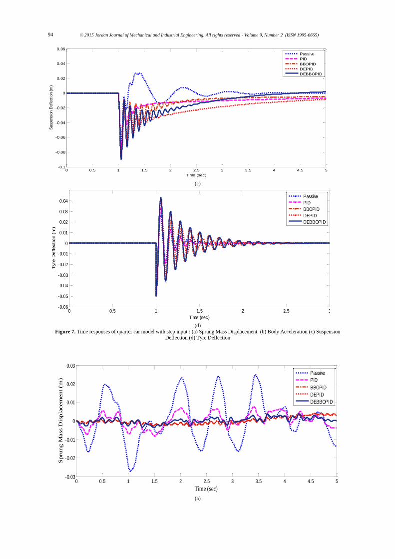
Figure 7. Time responses of quarter car model with step input : (a) Sprung Mass Displacement (b) Body Acceleration (c) Suspension Deflection (d) Tyre Deflection
0 0.5 1 1.5 2 2.5 3 3.5 4 4.5 5-0.03
-0.02
-0.01
0
0.01
0.02
0.03
Time (sec)
Spru
ng
Mass
Dis
pla
cem
en
t (m
)
Passive
PID
BBOPID
DEPID
DEBBOPID
(a)
© 2015 Jordan Journal of Mechanical and Industrial Engineering. All rights reserved - Volume 9, Number 2 (ISSN 1995-6665) 95
0 0.5 1 1.5 2 2.5 3 3.5 4 4.5 5-6
-4
-2
0
2
4
6
Time (sec)
Bod
y A
ccele
rati
on
(m
/s2)
Passive PID BBOPID DEPID DEBBOPID
(b)
0 0.5 1 1.5 2 2.5 3 3.5 4 4.5 5-0.06
-0.04
-0.02
0
0.02
0.04
0.06
Time (sec)
Suspensio
n D
efl
ecti
on (
m)
Passive PID BBOPID DEPID DEBBOPID
(c )
0 0.5 1 1.5 2 2.5 3 3.5 4 4.5 5-0.05
-0.04
-0.03
-0.02
-0.01
0
0.01
0.02
0.03
0.04
0.05
Time (sec)
Tyre
Defl
ecti
on (
m)
Passive PID BBOPID DEPID DEBBOPID
(d)
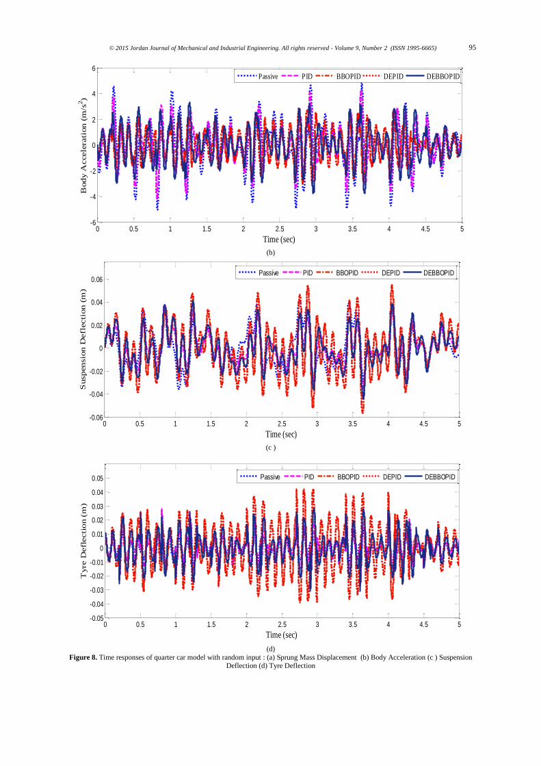
Figure 8. Time responses of quarter car model with random input : (a) Sprung Mass Displacement (b) Body Acceleration (c ) Suspension Deflection (d) Tyre Deflection
© 2015 Jordan Journal of Mechanical and Industrial Engineering. All rights reserved - Volume 9, Number 2 (ISSN 1995-6665) 96
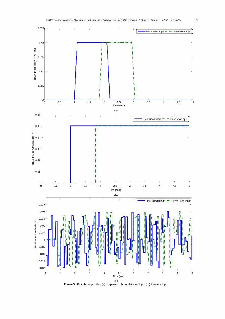
The simulation results of QC passive system, system
with PID, BBOPID, DEPID and DEBBOPID controllers
are shown in Figures 6, 7 and 8. (a) - (d).
It is clear from Figures 6, 7, 8. (a) and Figures 6, 7, 8.
(b) that the sprung mass displacement and vehicle body
acceleration is considerably reduced by the proposed
DEBBOPID controller. It guarantees the travelling comfort
to the passengers. Also Figure 6, 7, 8. (c) shows that the
suspension deflection with all the controllers are almost
the same. Figures 6, 7, 8. (d) illustrate the road holding
ability maintained by all the controllers. The tyre
displacement of active systems is higher than that of the
passive suspension system.
The RMS values of the time responses of the four
outputs with the three inputs are listed in Tables 2 to 4. It
is clear that the VASS using DEBBOPID controller is
useful for the betterment of the ride and travelling comfort
with a reduced body acceleration over PID controller, with
and without BBO or DE and the passive system.
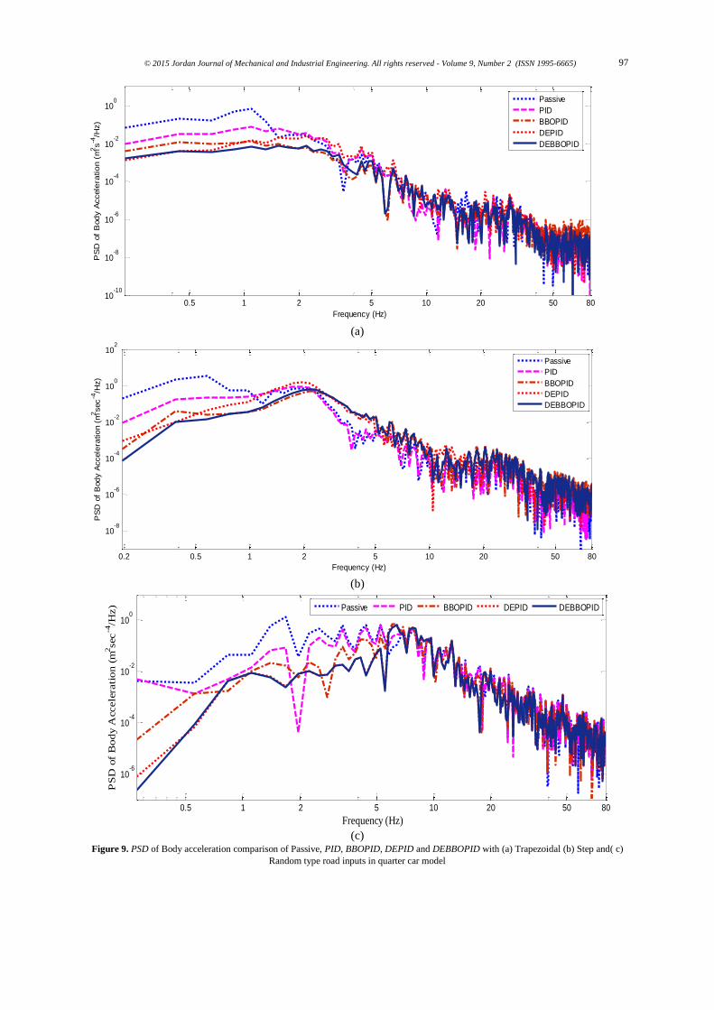
In the evaluation of the vehicle ride quality, the PSD
for the body acceleration as a function of frequency is of a
prime interest and is plotted for the passive system and that
with PID, BBOPID, DEPID and DEBBOPID controller
for the three different types of road inputs (Figure 9). It is
clear from the PSD plot that in the human sensitive
frequency range 4-8 Hz, compared to PID, BBOPID and
DEPID, DEBBOPID, reduces the vertical vibrations to a
great extent and improves the comfort of travelling when
subjected to trapezoidal road input.
Table 2. RMS values of the time responses of quarter car model with trapezoidal input
System Sprung Mass Displacement
(x10-3m)
Body
Acceleration
(x10-3m/s2)
Suspension
Deflection
(x10-3m)
Tyre
Deflection
(x10-4m)
Passive 10.61 336.6 4.81 6.168
PID 6.375 157.2 4.654 5.551
BBOPID 6.147 113.6 6.369 5.899
DEPID 4.294 98.0 7.574 7.278
DEBBOPID 5.575 82.3 7.741 6.563
Table 3. RMS values of the time responses of quarter car model with step input
System Sprung Mass Displacement
(x10-3m)
Body
Acceleration
(x10-3m/s2)
Suspension
Deflection
(x10-3m)
Tyre
Deflection
(x10-3m)
Passive 47.91 655 6.605 2.693
PID 40.36 531.9 9.842 2.903
BBOPID 41.11 526.8 11.32 4.432
DEPID 37.45 501.9 15.95 3.902
DEBBOPID 44.68 260.4 13.31 4.56
Table 4. RMS values of the time responses of quarter car model with random input
System Sprung Mass Displacement
(x10-3m)
Body
Acceleration
(x10-3m/s2)
Suspension
Deflection
(x10-3m)
Tyre
Deflection
(x10-3m)
Passive 28.43 2338.12 194.4 138.89
PID 21.94 1947.34 199.22 179.32
BBOPID 20.13 1802.53 201.5 193.04
DEPID 22.24 1732.521 203.45 200.13
DEBBOPID 21.35 1581.09 205.39 208.96
© 2015 Jordan Journal of Mechanical and Industrial Engineering. All rights reserved - Volume 9, Number 2 (ISSN 1995-6665) 97
0.5 1 2 5 10 20 50 8010
-10
10-8
10-6
10-4
10-2
100
Frequency (Hz)
PS
D o
f B
od
y A
ccele
ratio
n (
m2s
-4/H
z)
Passive
PID
BBOPID
DEPID
DEBBOPID
(a)
0.2 0.5 1 2 5 10 20 50 80
10-8
10-6
10-4
10-2
100
102
Frequency (Hz)
PS
D o
f B
od
y A
ccele
ratio
n (
m2sec
-4/H
z)
Passive
PID
BBOPID
DEPID
DEBBOPID
(b)
0.5 1 2 5 10 20 50 80
10-6
10-4
10-2
100
Frequency (Hz)
PS
D o
f B
od
y A
ccele
rati
on
(m
2sec
-4/H
z)
Passive PID BBOPID DEPID DEBBOPID
(c)
Figure 9. PSD of Body acceleration comparison of Passive, PID, BBOPID, DEPID and DEBBOPID with (a) Trapezoidal (b) Step and( c)
Random type road inputs in quarter car model
© 2015 Jordan Journal of Mechanical and Industrial Engineering. All rights reserved - Volume 9, Number 2 (ISSN 1995-6665) 98
0 0.5 1 1.5 2 2.5 3 3.5 4 4.5 5-0.03
-0.02
-0.01
0
0.01
0.02
0.03
Time (sec)
Bod
y A
ccele
rati
on
(m
/s2)
Passive
PID
BBOPID
DEPID
DEBBOPID
(a)
0 0.5 1 1.5 2 2.5 3 3.5 4 4.5 5-0.04
-0.03
-0.02
-0.01
0
0.01
0.02
0.03
0.04
0.05
Time (sec)
Bod
y A
ccele
rati
on
(m
/s2)
Passive
PID
BBOPID
DEPID
DEBBOPID
(b)
0 1 2 3 4 5 6 7 8 9 10-0.1
-0.08
-0.06
-0.04
-0.02
0
0.02
0.04
0.06
0.08
0.1
Time (sec)
Bod
y A
ccele
rati
on
(m
/s2)
Passive
PID
BBOPID
DEPID
DEBBOPID
(c)
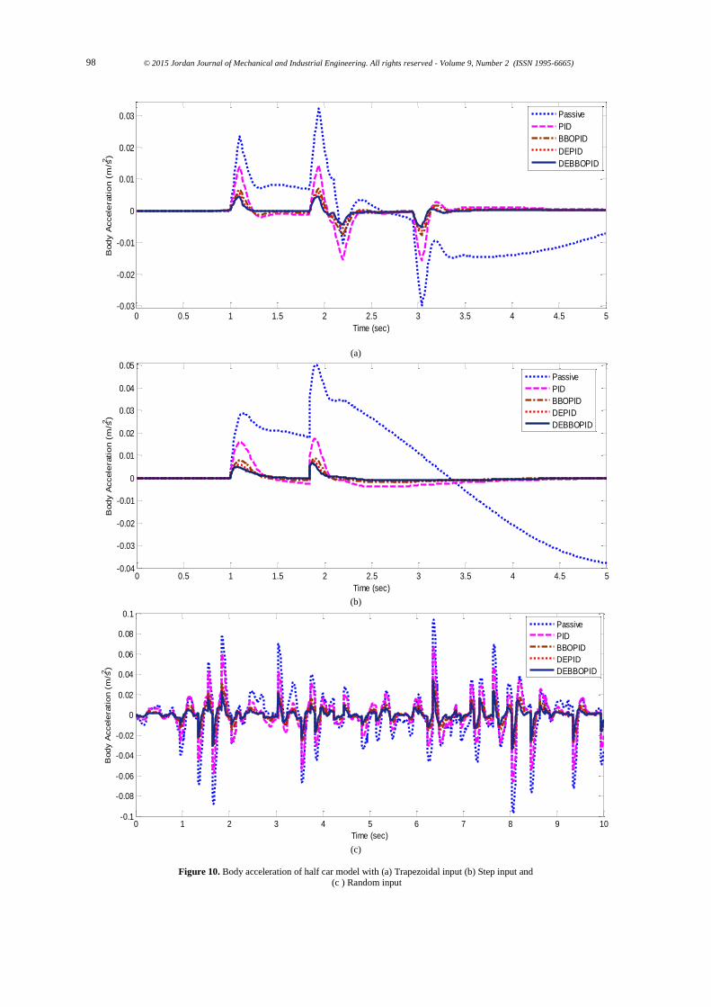
Figure 10. Body acceleration of half car model with (a) Trapezoidal input (b) Step input and (c ) Random input
© 2015 Jordan Journal of Mechanical and Industrial Engineering. All rights reserved - Volume 9, Number 2 (ISSN 1995-6665) 99
0.2 0.5 1 5 10 15 20
10-12
10-10
10-8
10-6
10-4
Frequency (Hz)
PS
D o
f B
od
y a
cce
lera
tio
n (
m2sec
-4/H
z)
Passive
PID
BBOPID
DEPID
DEBBOPID
(a)
0.2 0.5 1 5 10 15 20
10-12
10-10
10-8
10-6
10-4
10-2
Frequency (Hz)
PS
D o
f B
od
y a
cce
lera
ion
(m
2sec
-4/H
z)
Passive
PID
BBOPID
DEPID
DEBBOPID
(b)
0.2 0.5 1 5 10 15 20
10-10
10-8
10-6
10-4
Frequency (Hz)
PS
D o
f B
od
y a
cce
lera
tio
n (
m2sec
-4/H
z)
Passive PID BBOPID DEPID DEBBOPID
(c)
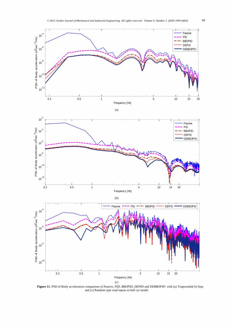
Figure 11. PSD of Body acceleration comparison of Passive, PID, BBOPID, DEPID and DEBBOPID with (a) Trapezoidal( b) Step and (c) Random type road inputs in half car model
© 2015 Jordan Journal of Mechanical and Industrial Engineering. All rights reserved - Volume 9, Number 2 (ISSN 1995-6665) 100
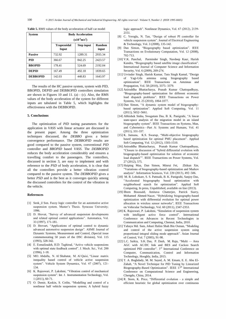
Table 5. RMS values of the body acceleration of half car model
System Body Acceleration
(x10-6m/s2)
Trapezoidal
Input
Step input Random
input
Passive 732.92 1289.31 2935.34
PID 366.67 842.25 2423.57
BBOPID 178.41 524.69 2192.04
DEPID 167.49 492.18 1839.65
DEBBOPID 142.03 448.83 1643.97
The results of the HC passive system, system with PID,
BBOPID, DEPID and DEBBOPID controllers simulation
are shown in Figures 10 and 11. (a) - (c). Also, the RMS
values of the body acceleration of the system for different
inputs are tabulated in Table 5, which highlights the
effectiveness with the DEBBOPID.
5. Conclusions
The optimization of PID tuning parameters for the
application in VASS with linear actuator are discussed in
the present paper. Among the three optimization
techniques discussed, the DEBBO gives a better
convergence performance. The DEBBOPID results are
good compared to the passive system, conventional PID
controller and BBOPID based VASS. The DEBBOPID
reduces the body acceleration considerably and ensures a
travelling comfort to the passengers. The controllers,
discussed in section 3, are easy to implement and with
reference to the PSD of body acceleration, it is clear that
all the controllers provide a better vibration control
compared to the passive system. The DEBBOPID gives a
better PSD and is the best as it converges quickly among
the discussed controllers for the control of the vibration in
the vehicle.
References
[1] Seok_il Son. Fuzzy logic controller for an automotive active
suspension system. Master’s Thesis. Syracuse University;
1996.
[2] D. Hrovat, “Survey of advanced suspension developments
and related optimal control applications”. Automatica, Vol.
33 (1997), 171-181.
[3] D. Hrovart, “Applications of optimal control to dynamic
advanced automotive suspension design”. ASME Journal of
Dynamic Systems, Measurement and Control, (Special issue
commemorating 50 years of the DSC division), Vol. 115
(1993), 328-342.
[4] E. Esmailzadeh, H.D. Taghirad, “Active vehicle suspensions
with optimal state feedback control”. J. Mech. Sci., Vol. 200
(1996), 1-18.
[5] MO. Abdalla, N. Al Shabatat, M. Al Qaisi, “Linear matrix
inequality based control of vehicle active suspension
system”. Vehicle System Dynamics, Vol. 47 (2007), 121-
134.
[6] K. Rajeswari, P. Lakshmi, “Vibration control of mechanical
suspension system”. Int. J. Instrumentation Technology, Vol.
1 (2011), 60-71.
[7] O. Demir, Keskin, S. Cetlin, “Modelling and control of a
nonlinear half vehicle suspension system; A hybrid fuzzy
logic approach”. Nonlinear Dynamics, Vol. 67 (2012), 2139-
2151.
[8] C. Yeroglu, N. Tan, “Design of robust PI controller for
vehicle suspension system”. Journal of Electrical Engineering
& Technology, Vol. 3 (2008), 135-142.
[9] Dan Simon, “Biogeography based optimization”. IEEE
Transactions on Evolutionary Computation, Vol. 12 (2008),
702-713.
[10] V.K. Panchal, Parminder Singh, Navdeep Kaur, Harish
Kundra, “Biogeography based satellite image classification”.
International Journal of Computer Science and Information
Security, Vol. 6 (2009), 269-274.
[11] Urvinder Singh, Harish Kumar, Tara Singh Kamal, “Design
of Yagi-Uda antenna using biogeography based
optimization”. IEEE Transactions on Antennas and
Propagation, Vol. 58 (2010), 3375- 3379.
[12] Aniruddha Bhattacharya, Pranab Kumar Chattopadhyay,
“Biogeography-based optimization for different economic
load dispatch problems”. IEEE Transactions on Power
Systems, Vol. 25 (2010), 1064-1077.
[13] Dan Simon, “A dynamic system model of biogeography-
based optimization”. Applied Soft Computing, Vol. 11
(2011), 5652–5661.
[14] Abhishek Sinha, Swagatam Das, B. K. Panigrahi, “A linear
state-space analysis of the migration model in an island
biogeography system”. IEEE Transactions on Systems, Man,
and Cybernetics—Part A: Systems and Humans, Vol. 41
(2011), 331-337.
[15] K. Jamuna, K.S. Swarup, “Multi-objective biogeography
based optimization for optimal PMU placement”. Applied
Soft Computing, Vol. 12 (2012), 1503-1510.
[16] Aniruddha Bhattacharya, Pranab Kumar Chattopadhyay,
“Closure to discussion of “hybrid differential evolution with
biogeography-based optimization for solution of economic
load dispatch””. IEEE Transactions on Power Systems, Vol.
27 (2012), 575.
[17] Haiping Maa, Dan Simon, Minrui Fei, Zhikun Xie,
“Variations of biogeography-based optimization and Markov
analysis”. Information Sciences, Vol. 220 (2013), 492–506.
[18] M. R. Lohokare, S. S. Pattnaik, B. K. Panigrahi, Sanjoy Das,
“Accelerated biogeography based optimization with
neighborhood search for optimization”. Applied Soft
Computing, In press, Unpublished, available on line (2013).
[19] Ilhem Boussaïd, Amitava Chatterjee, Patrick Siarry,
Mohamed Ahmed-Nacer, “Hybridizing biogeography-based
optimization with differential evolution for optimal power
allocation in wireless sensor networks”, IEEE Transactions
on Vehicular Technology, Vol. 60 (2011), 2347-2353.
[20] K. Rajeswari, P. Lakshmi, “Simulation of suspension system
with intelligent active force control”. International
Conference on Advances in Recent Technologies in
Communication and Computing, Chennai, India, 2010.
[21] Yahaya Md. Sam, Johari Halim Shah Bin Osman, “Modeling
and control of the active suspension system using
proportional integral sliding mode approach”. Asian Journal
of Control, Vol. 7 (2005), 91-98.
[22] L.C. Saikia, S.K. Das, P. Dash, M. Raju, “Multi — Area
AGC with AC/DC link and BES and Cuckoo Search
optimized PID controller”. 3rd International Conference on
Computer, Communication, Control and Information
Technology, Hooghly, India, 2015.
[23] T. A. Boghdady, M. M. Sayed, A. M. Emam, E. E. Abu El-
Zahab, “A Novel Technique for PID Tuning by Linearized
Biogeography-Based Optimization”. IEEE 17th International
Conference on Computational Science and Engineering,
Chengdu, China, 2014.
[24] R. Storn, K. Price, “Differential evolution - a simple and
efficient heuristic for global optimization over continuous

© 2015 Jordan Journal of Mechanical and Industrial Engineering. All rights reserved - Volume 9, Number 2 (ISSN 1995-6665) 101
spaces”. Journal of Global Optimization, Vol. 11 (1997),
341-359.
[25] Rukmini V Kasarapu, Vijaya B. Vommi, “Economic design
of joint X and R control charts using differential evolution”.
Jordan Journal of Mechanical and Industrial Engineering,
Vol. 5, (2011) No. 2, 149-160.
[26] Aniruddha Bhattacharya, P.K. Chattopadhyay, “Hybrid
differential evolution with biogeography-based optimization
algorithm for solution of economic emission load dispatch
problems”. Expert Systems with Applications, Vol. 38
(2011), 14001–14010.
[27] R. Kalaivani, P. Lakshmi, K. Sudhagar, “Hybrid (DEBBO)
Fuzzy Logic Controller for quarter car model: DEBBOFLC
for Quarter Car model”. UKACC International Conference
on Control (CONTROL), Loughborough, U.K., 2014.