jet simulation facility using the ludwieg tube principle

5TH EUROPEAN CONFERENCE FOR AERONAUTICS AND SPACE SCIENCES (EUCASS)

Copyright 2013 by First Author and Second Author. Published by the EUCASS association with permission.

Jet Simulation Facility using the Ludwieg Tube Principle

S. Stephan*, R. Radespiel * and R. Müller-Eigner**

* Institute of Fluid Mechanics, Technische Universität Braunschweig,

Hermann-Blenk-Str. 37, 38108 Braunschweig, Germany

** HST GmbH

Max-Planck-Str. 19, 37191 Katlenburg-Lindau, Germany

Abstract Afterbody flow phenomena represent a major source of uncertainties in the design of a launcher. Therefore there is a demand for measuring such flows in a wind tunnel. As a new approach to propulsive jet simulation a new jet facility was integrated into a hypersonic wind tunnel. This jet simulation facility resembles an Ariane 5 launcher. The design of the facility and first experimental results are reported. This includes measurements of pressure, temperature and Mach number distribution. Also the unsteady pressure distribution on the rocket base and on the nozzle fairing is analysed.

1. Introduction

The interest in jet simulation is motivated by the need for experimental data in the area of afterbody flow phenomena. At atmospheric rocket flights there are a multitude of interactions between free stream and jet. These interactions influence the flight characteristics. While a number of investigations are reported in the literature on missiles, the literature on launchers with jet simulation is sparse. For example Peters [1], [2] researched the effect of the boattail drag for different jet simulation parameters by variation of the boattail, the nozzle exit to throat ratio, the jet temperatures and the gas composition. Kumar [3] presented investigations in boattail separated flows relevant to launch vehicle configurations. This included mean and fluctuation pressure measurements. The investigations were made at transonic speeds ranging from Ma = 0.7 to 1.2 and various boattail angles and diameter ratios. Investigations of the Ariane 5 European launcher afterbody at a scale of 0.01 have been conducted by Reijasse [4]. The first stage including the center engine and boosters was studied in a blow down wind tunnel at Ma = 4. The jet was simulated with cold high pressure air, which was expanded to resemble flight at an altitude of 30km. As a result the complex flow field consisting of supersonic, subsonic and reverse flows was determined. In this paper a new jet simulation facility for cost-effective research on turbulent afterbody flows is presented. The characteristic properties such as velocity ratio can be adjusted to match real flight conditions. The jet simulation facility in its current stage can be run in stagnant air and also in hypersonic flow. The jet simulation facility is of the Ludwieg tube blow down type. Ludwieg tubes work with a fast acting valve so that a good flow quality can be obtained at low operational cost. Detailed information about Ludwieg tubes with fast acting valves are presented by Koppenwallner [5]. Usually Ludwieg tubes are cold blow-down facilities. In the present case the storage tube used for jet simulation can be heated up to 900K and gas of low molar mass can be employed to adjust characteristic jet properties. The new jet simulation facility is integrated into a large Ludwieg tube that generates the hypersonic flow field around the afterbody. The overall wind tunnel configuration is rather simple and it allows for cost-efficient but high-quality research typically performed by universities.

2. Design Approach of Jet Simulation

For simulating rocket afterbody flows in wind tunnel facilities it is important to reproduce the mayor rocket plume flow parameters. A review of various techniques for simulation of jet exhaust in ground testing facilities is given by Pindzola [6]. The scaling of the rocket plume for the jet simulation facility used in the present work is based on discussions with industry in rocket propulsion [7]. The launcher to be scaled is the Ariane 5 with a Vulcain 2 rocket motor at an altitude of 50 km. The free stream conditions at flight and in the wind tunnel are shown in Tab. 1.

S.Stephan, R. Radespiel, R. Müller-Eigner

2

Table 1: Free-stream conditions for the hypersonic wind tunnel HLB and the Ariane 5 trajectory

HLB Ariane 5

p∞[bar] 1.3 x 10-2 7.6 x 10-4

T∞[K] 58 271

Ma∞ 5.9 5.3

The easiest approach would be a geometric scaling, but for wind tunnel simulations that is very difficult approach. Rocket motors used in launchers have hot rocket plumes with total temperatures up to 3500K. This high temperature would create extreme heat loads on the wind tunnel models and limit the use of sensors and the infrastructure cost are extremely high. Hence jet simulations in wind tunnels usually employ cold plumes. But for physics based ground simulation two major afterbody flow mechanisms are important and should be considered. One mechanism is flow displacement by plume shape. The plume shape affects the positions of the shear layer and the plume shock. It mainly depends on the ratio of nozzle exit pressure to static pressure in the free-stream. The second mechanism is flow entrainment into the plume. The entrainment describes the effect of the shear layer to entrain gas from the base flow. Entrainment results from turbulent mixing and this is associated with the large turbulent structures in the afterbody flow. Simulation of turbulent mixing is therefore needed to represent buffet flow phenomena at the rocket afterbody. The differences between wind tunnel and rocket operation plume conditions affect the similarity parameters for entrainment such as the velocity ratio. The low total temperature used in wind tunnel facilities reduces the exhaust velocity. Varying the specific heat ratio of the plume fluid affects the exit Mach number and the flow expansion. The exhaust velocity is also affected by different gas molar masses. Finally, a higher density of the jet flow will affect the shear layer growth. In conclusion, entrainment and growth of mixing layers are governed by two important parameters. The first is the shear layer driving velocity to plume velocity ratio, (uP − u∞)/uP. This parameter is expected to govern turbulence production in the shear layer and unsteadiness of the afterbody flow. The second parameter is the momentum ratio (ρP · uP )/(ρ∞ · u∞). This parameter will affect the growth of the shear layer and its position relative to the nozzle axis. Note that the plume velocity is not equal to the nozzle exit velocity. Rather, the plume velocity is the velocity in the region between the shear layer and the barrel shock of the underexpanded jet. The velocity ratio and the momentum ratio should be varied in significant amounts by using the facility to make experiments representative. For assessing the potential of the wind tunnel set-up a simple estimate is to observe the plume velocity for expansions to p = 0. In this case the plume velocity uP is replaced by umax = [(2κ)/(κ−1)( ℜ Tt)/MMol]

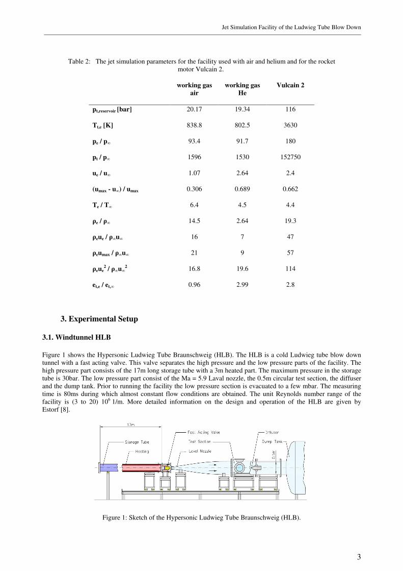
-1/2. This formula shows that the maximum velocity depends on the molar mass, the specific heat ratio and the total temperature. Therefore by changing the gas composition the velocity can be modified. The maximum velocity for the Vulcain 2 (H2/O2 combustion; κ= 1.2; MMol = 13.5 g/mol) is umax, Vulcain 2 = 5086 m/s at Tt = 3500K. Heated air (κ= 1.4; MMol= 29 g/mol) reaches 25 % and heated helium (κ= 1.67; MMol= 4 g/mol) 56 % of umax, Vulcain 2 at Tt = 800K. Note that chemical effects in the jet may not be well represented by using gases with different specific heat ratio and different molar mass. In Tab. 2 the important ratios for jet simulation for the Vulcain 2 and for the jet simulation facility with different working gases are shown. The first, nozzle to free-stream pressure ratio pe/p∞, shows the degree of underexpansion. The Vulcain 2 expansion is twice as large as in the present simulation facility. The second ratio is the total nozzle to free stream pressure ratio pt/p∞. This ratio is necessarily much smaller in wind tunnel facilities without high-pressure combustion. The nozzle exit velocity to free stream velocity ratio ue/u∞ is much too small compared to Vulcain 2 if air is used as a jet fluid. When helium is used as working gas the velocity ratios are quite similar. Also full simulation capability of the (umax−u∞)/umax ratio and the nozzle exit to free stream temperature ratio is achieved. The density and the momentum ratios exhibit larger differences for both working gases as mentioned in the table. Especially for helium there are large differences, because of much lower helium molar mass. This should move the high-speed boundary of the mixing layer somewhat closer to the nozzle axis, as compared to Vulcain 2. The kinetic energy ratio ρe ue

2 / ρ∞ u∞2 is

6 times smaller for both working gas compared to the Vulcain 2. But the total energy ratio et,e/et,∞ ( kinetic energy and inner energy ) is roughly similar for helium as working gas. Note that the molecular viscosity at high Reynoldsnumbers is not important for shear flow simulation.

Jet Simulation Facility of the Ludwieg Tube Blow Down

3

Table 2: The jet simulation parameters for the facility used with air and helium and for the rocket motor Vulcain 2.

working gas

air

working gas

He

Vulcain 2

pt,reservoir [bar] 20.17 19.34 116

Tt,e [K] 838.8 802.5 3630

pe / p∞ 93.4 91.7 180

pt / p∞ 1596 1530 152750

ue / u∞ 1.07 2.64 2.4

(umax - u∞) / umax 0.306 0.689 0.662

Te / T∞ 6.4 4.5 4.4

ρe / ρ∞ 14.5 2.64 19.3

ρeue / ρ∞u∞ 16 7 47

ρeumax / ρ∞u∞ 21 9 57

ρeue2 / ρ∞u∞

2 16.8 19.6 114

et,e / et,∞ 0.96 2.99 2.8

3. Experimental Setup

3.1. Windtunnel HLB

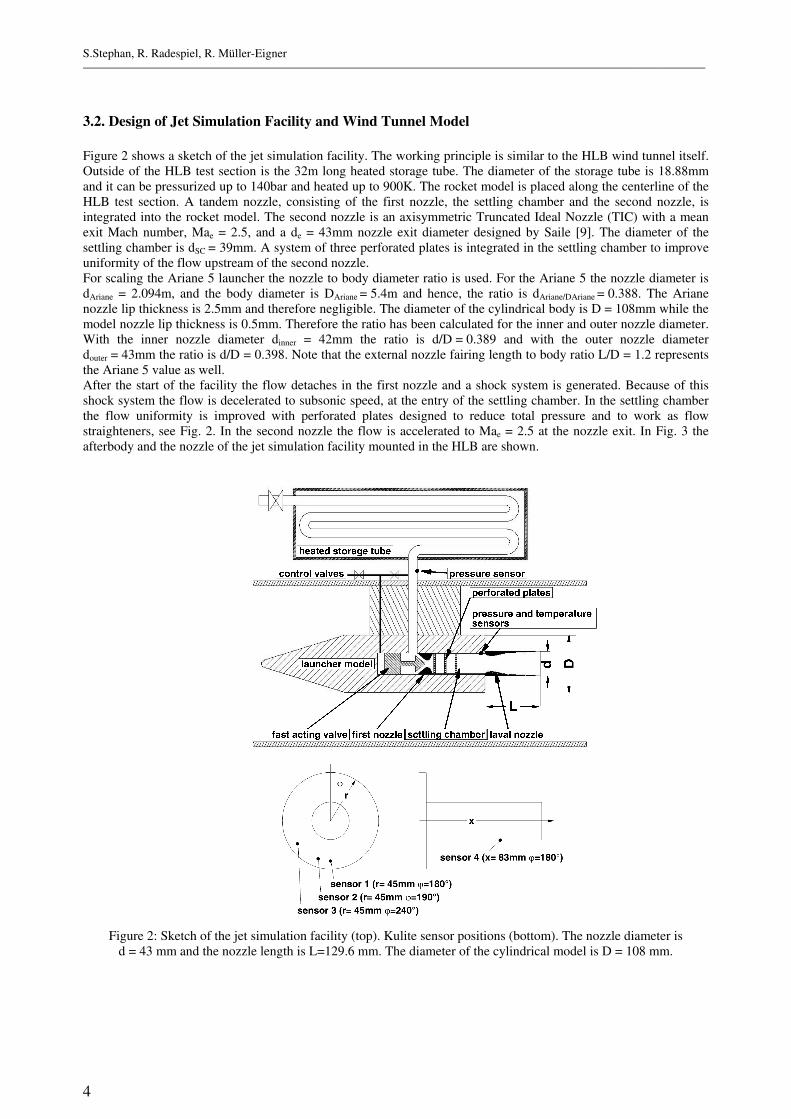
Figure 1 shows the Hypersonic Ludwieg Tube Braunschweig (HLB). The HLB is a cold Ludwieg tube blow down tunnel with a fast acting valve. This valve separates the high pressure and the low pressure parts of the facility. The high pressure part consists of the 17m long storage tube with a 3m heated part. The maximum pressure in the storage tube is 30bar. The low pressure part consist of the Ma = 5.9 Laval nozzle, the 0.5m circular test section, the diffuser and the dump tank. Prior to running the facility the low pressure section is evacuated to a few mbar. The measuring time is 80ms during which almost constant flow conditions are obtained. The unit Reynolds number range of the facility is (3 to 20) 106 1/m. More detailed information on the design and operation of the HLB are given by Estorf [8].

Figure 1: Sketch of the Hypersonic Ludwieg Tube Braunschweig (HLB).


4

3.2. Design of Jet Simulation Facility and Wind Tunnel Model

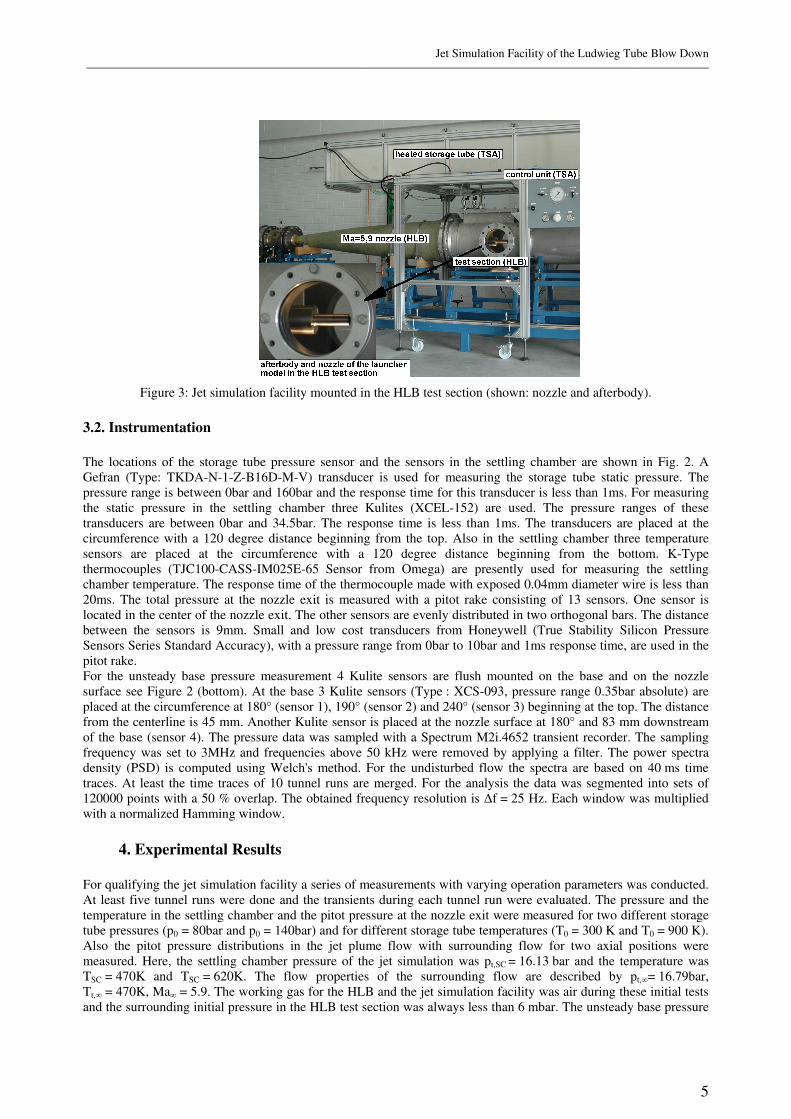
Figure 2 shows a sketch of the jet simulation facility. The working principle is similar to the HLB wind tunnel itself. Outside of the HLB test section is the 32m long heated storage tube. The diameter of the storage tube is 18.88mm and it can be pressurized up to 140bar and heated up to 900K. The rocket model is placed along the centerline of the HLB test section. A tandem nozzle, consisting of the first nozzle, the settling chamber and the second nozzle, is integrated into the rocket model. The second nozzle is an axisymmetric Truncated Ideal Nozzle (TIC) with a mean exit Mach number, Mae = 2.5, and a de = 43mm nozzle exit diameter designed by Saile [9]. The diameter of the settling chamber is dSC = 39mm. A system of three perforated plates is integrated in the settling chamber to improve uniformity of the flow upstream of the second nozzle. For scaling the Ariane 5 launcher the nozzle to body diameter ratio is used. For the Ariane 5 the nozzle diameter is dAriane = 2.094m, and the body diameter is DAriane = 5.4m and hence, the ratio is dAriane/DAriane = 0.388. The Ariane nozzle lip thickness is 2.5mm and therefore negligible. The diameter of the cylindrical body is D = 108mm while the model nozzle lip thickness is 0.5mm. Therefore the ratio has been calculated for the inner and outer nozzle diameter. With the inner nozzle diameter dinner = 42mm the ratio is d/D = 0.389 and with the outer nozzle diameter douter = 43mm the ratio is d/D = 0.398. Note that the external nozzle fairing length to body ratio L/D = 1.2 represents the Ariane 5 value as well. After the start of the facility the flow detaches in the first nozzle and a shock system is generated. Because of this shock system the flow is decelerated to subsonic speed, at the entry of the settling chamber. In the settling chamber the flow uniformity is improved with perforated plates designed to reduce total pressure and to work as flow straighteners, see Fig. 2. In the second nozzle the flow is accelerated to Mae = 2.5 at the nozzle exit. In Fig. 3 the afterbody and the nozzle of the jet simulation facility mounted in the HLB are shown.

Figure 2: Sketch of the jet simulation facility (top). Kulite sensor positions (bottom). The nozzle diameter is d = 43 mm and the nozzle length is L=129.6 mm. The diameter of the cylindrical model is D = 108 mm.


5

Figure 3: Jet simulation facility mounted in the HLB test section (shown: nozzle and afterbody).

3.2. Instrumentation

The locations of the storage tube pressure sensor and the sensors in the settling chamber are shown in Fig. 2. A Gefran (Type: TKDA-N-1-Z-B16D-M-V) transducer is used for measuring the storage tube static pressure. The pressure range is between 0bar and 160bar and the response time for this transducer is less than 1ms. For measuring the static pressure in the settling chamber three Kulites (XCEL-152) are used. The pressure ranges of these transducers are between 0bar and 34.5bar. The response time is less than 1ms. The transducers are placed at the circumference with a 120 degree distance beginning from the top. Also in the settling chamber three temperature sensors are placed at the circumference with a 120 degree distance beginning from the bottom. K-Type thermocouples (TJC100-CASS-IM025E-65 Sensor from Omega) are presently used for measuring the settling chamber temperature. The response time of the thermocouple made with exposed 0.04mm diameter wire is less than 20ms. The total pressure at the nozzle exit is measured with a pitot rake consisting of 13 sensors. One sensor is located in the center of the nozzle exit. The other sensors are evenly distributed in two orthogonal bars. The distance between the sensors is 9mm. Small and low cost transducers from Honeywell (True Stability Silicon Pressure Sensors Series Standard Accuracy), with a pressure range from 0bar to 10bar and 1ms response time, are used in the pitot rake. For the unsteady base pressure measurement 4 Kulite sensors are flush mounted on the base and on the nozzle surface see Figure 2 (bottom). At the base 3 Kulite sensors (Type : XCS-093, pressure range 0.35bar absolute) are placed at the circumference at 180° (sensor 1), 190° (sensor 2) and 240° (sensor 3) beginning at the top. The distance from the centerline is 45 mm. Another Kulite sensor is placed at the nozzle surface at 180° and 83 mm downstream of the base (sensor 4). The pressure data was sampled with a Spectrum M2i.4652 transient recorder. The sampling frequency was set to 3MHz and frequencies above 50 kHz were removed by applying a filter. The power spectra density (PSD) is computed using Welch's method. For the undisturbed flow the spectra are based on 40 ms time traces. At least the time traces of 10 tunnel runs are merged. For the analysis the data was segmented into sets of 120000 points with a 50 % overlap. The obtained frequency resolution is ∆f = 25 Hz. Each window was multiplied with a normalized Hamming window.

4. Experimental Results

For qualifying the jet simulation facility a series of measurements with varying operation parameters was conducted. At least five tunnel runs were done and the transients during each tunnel run were evaluated. The pressure and the temperature in the settling chamber and the pitot pressure at the nozzle exit were measured for two different storage tube pressures (p0 = 80bar and p0 = 140bar) and for different storage tube temperatures (T0 = 300 K and T0 = 900 K). Also the pitot pressure distributions in the jet plume flow with surrounding flow for two axial positions were measured. Here, the settling chamber pressure of the jet simulation was pt,SC = 16.13 bar and the temperature was TSC = 470K and TSC = 620K. The flow properties of the surrounding flow are described by pt,∞= 16.79bar, Tt,∞ = 470K, Ma∞ = 5.9. The working gas for the HLB and the jet simulation facility was air during these initial tests and the surrounding initial pressure in the HLB test section was always less than 6 mbar. The unsteady base pressure


6

was measured with and without jet flow. The total temperatures were varied as 300 K (pt,SC = 19.2 bar), 470 K (pt,SC = 17.1 bar), and 620 K (pt,SC = 16.13 bar).

4.1. Flow Measurements in Storage Tube and Settling Chamber

Figure 4 shows the static storage tube pressure for different initial storage tube pressures and different temperatures. Right after the opening of the fast acting valve (t = 0 ms) there is a pressure loss of 24 % for low temperatures and of 26 % for high temperatures because of the unsteady starting process. During the measuring time of 100 ms the pressure drops further by 15 %. This pressure loss is described by Koppenwallner [10]. Koppenwallner investigated Ludwieg tubes with Laval nozzles of different area ratios. He found that the pressure loss over the measuring time depends on the storage tube Mach number. With rising Mach number the pressure loss increases. The pressure drop of the present facility with a storage tube Mach number of 0.2 is in good agreement with the results of reference [10].

Figure 4: Static storage tube pressure for different initial storage tube pressures and different storage tube

temperatures.

Figure 5: Settling chamber pressure to storage tube pressure during runtime for different temperatures.


7

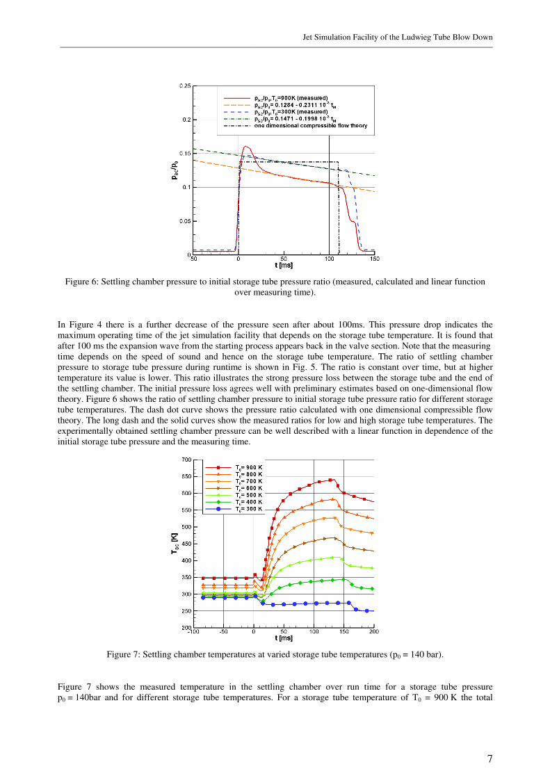
Figure 6: Settling chamber pressure to initial storage tube pressure ratio (measured, calculated and linear function over measuring time).

In Figure 4 there is a further decrease of the pressure seen after about 100ms. This pressure drop indicates the maximum operating time of the jet simulation facility that depends on the storage tube temperature. It is found that after 100 ms the expansion wave from the starting process appears back in the valve section. Note that the measuring time depends on the speed of sound and hence on the storage tube temperature. The ratio of settling chamber pressure to storage tube pressure during runtime is shown in Fig. 5. The ratio is constant over time, but at higher temperature its value is lower. This ratio illustrates the strong pressure loss between the storage tube and the end of the settling chamber. The initial pressure loss agrees well with preliminary estimates based on one-dimensional flow theory. Figure 6 shows the ratio of settling chamber pressure to initial storage tube pressure ratio for different storage tube temperatures. The dash dot curve shows the pressure ratio calculated with one dimensional compressible flow theory. The long dash and the solid curves show the measured ratios for low and high storage tube temperatures. The experimentally obtained settling chamber pressure can be well described with a linear function in dependence of the initial storage tube pressure and the measuring time.

Figure 7: Settling chamber temperatures at varied storage tube temperatures (p0 = 140 bar).

Figure 7 shows the measured temperature in the settling chamber over run time for a storage tube pressure p0 = 140bar and for different storage tube temperatures. For a storage tube temperature of T0 = 900 K the total


8

temperature in the settling chamber reaches TSC = 620 K after 80ms. We find that for high storage tube temperatures the settling chamber does not reach a constant level. This could be caused by heat transfer in the unheated support tube that connects the model with the heated storage tube. For future improved measurements this part should be isolated and heated as well. Figure 8 shows the settling chamber total pressure pt,SC as a function of storage tube temperature T0 and storage tube pressure taken at 80ms after the facility start. With higher storage tube temperatures the settling chamber pressure decreases. Figure 9 displays the settling chamber temperature as function of the storage tube temperature for storage tube pressures from 70bar to 140bar (80ms after the facility starts). Up to T0 = 700K the variance of the settling chamber temperature is ±10K. For higher storage tube temperatures the temperatures variances increase.

Figure 8: Settling chamber pressure for different storage tube temperatures at 80 ms.

Figure 9: Settling chamber temperatures for different storage tube temperatures at 80 ms.

4.2. Flow Measurements of Propulsive Jet

Figure 10 shows the ratio of nozzle exit pitot pressure to settling chamber total pressure ratio. The pitot pressures are measured in the center of the nozzle exit as an average over 5 tunnel runs. The values are almost constant over the measuring time. We find

900K). (Tp · 0.0044) (0.4357 p

300K) (Tp · 0.0033) (0.4440 p

0SCt,CPitot,

0SCt,CPitot,

=±=

=±= (1)


9

Figure 10: Pitot pressure in the center of the rocket nozzle exit.

Figure 11: Pitot pressure distribution along the vertical nozzle exit.

Figure 11 shows the vertical pitot pressure distribution across the nozzle exit. The distribution indicates a symmetrical jet flow. Also it is shown, that the pressure increases in radial direction. In Figure 12 the Mach number distribution calculated with the Rayleigh pitot formula is shown. Also the Mach number distribution obtained from RANS computations of the same nozzle by Saile [9] is included. The Figure shows a good agreement between the computed and the measured Mach number distribution. In Figs. 13 and 14 the pitot pressure distributions of the plume flow at the axial positions x/d = 2 and x/d = 3 are shown. The total pressure in the settling chamber was pt,SC = 16.13 bar and the settling chamber temperatures were varied between 470 K and 620 K. The flow properties of the surrounding flow were pt,∞ = 16.79 bar, T∞ = 470 K and Ma∞ = 5.9. Both facilities were synchronized to overlap their measuring windows. The values used for the evaluation are the mean values between 60 ms and 80 ms after the start of the jet simulation facility. Figure 13 shows the pitot pressure distribution of the plume flow at the axial position x/d = 2. Note that the differences between the pitot pressure distributions at different temperatures may have also been affected by locally large variations from run to run in the mixing region at z/D = ± ( 0.4 to 1) that divides the jet flow from the surrounding flow. In Figure 14 the pitot pressure distribution for the axial position x/d = 3 is shown. These measurements were only conducted for the lower part of the jet plume.


10

Figure 12: Pitot pressure distribution in the vertical plane of symmetry at the nozzle exit.

Figure 13: Pitot pressure distribution in jet plume at x/d = 2.

Figure 14: Pitot pressure distribution in jet plume x/d = 3.


11

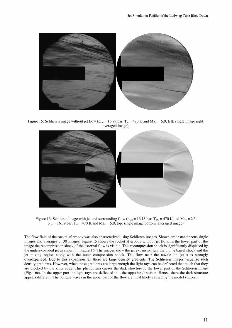
Figure 15: Schlieren image without jet flow (pt,∞ = 16.79 bar, T∞ = 470 K and Ma∞ = 5.9, left: single image right: averaged image).

Figure 16: Schlieren image with jet and surrounding flow (pt,sc = 16.13 bar, TSC = 470 K and Mae = 2.5, pt,∞ = 16.79 bar, T∞ = 470 K and Ma∞ = 5.9, top: single image bottom: averaged image).

The flow field of the rocket afterbody was also characterized using Schlieren images. Shown are instantaneous single images and averages of 30 images. Figure 15 shows the rocket afterbody without jet flow. In the lower part of the image the recompression shock of the external flow is visible. This recompression shock is significantly displaced by the underexpanded jet as shown in Figure 16. The images show the jet expansion fan, the plume barrel shock and the jet mixing region along with the outer compression shock. The flow near the nozzle lip (exit) is strongly overexpanded. Due to this expansion fan there are large density gradients. The Schlieren images visualize such density gradients. However, when these gradients are large enough the light rays can be deflected that much that they are blocked by the knife edge. This phenomena causes the dark structure in the lower part of the Schlieren image (Fig. 16a). In the upper part the light rays are deflected into the opposite direction. Hence, there the dark structure appears different. The oblique waves in the upper part of the flow are most likely caused by the model support.


12

4.2. Unsteady Base Flow Measurements

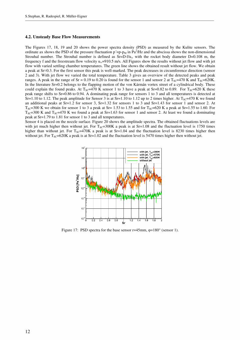
The Figures 17, 18, 19 and 20 shows the power spectra density (PSD) as measured by the Kulite sensors. The ordinate ax shows the PSD of the pressure fluctuation p´=p-pM in Pa2/Hz and the abscissa shows the non-dimensional Strouhal number. The Strouhal number is defined as Sr=D·f/u∞ with the rocket body diameter D=0.108 m, the frequency f and the freestream flow velocity u∞=910.5 m/s. All Figures show the results without jet flow and with jet flow with varied settling chamber temperatures. The green line shows the obtained result without jet flow. We obtain a peak at Sr≈0.3. For the first sensor this peak is well-marked. The peak decreases in circumference direction (sensor 2 and 3). With jet flow we varied the total temperature. Table 3 gives an overview of the detected peaks and peak ranges. A peak in the range of Sr = 0.19 to 0.20 is found for the sensor 1 and sensor 2 at TSC=470 K and TSC=620K. In the literature Sr=0.2 belongs to the flapping motion of the von Kármán vortex street of a cylindrical body. These could explain the found peaks. At TSC=470 K sensor 1 to 3 have a peak at Sr=0.82 to 0.89. For TSC=620 K these peak range shifts to Sr=0.86 to 0.94. A dominating peak range for sensors 1 to 3 and all temperatures is detected at Sr=1.10 to 1.12. The peak amplitude for Sensor 3 is at Sr=1.10 to 1.12 up to 2 times higher. At TSC=470 K we found an additional peaks at Sr=1.2 for sensor 3, Sr=1.32 for sensors 1 to 3 and Sr=1.43 for sensor 1 and sensor 2. At TSC=300 K we obtain for sensor 1 to 3 a peak at Sr= 1.53 to 1.55 and for TSC=620 K a peak at Sr=1.55 to 1.60. For TSC=300 K and TSC=470 K we found a peak at Sr=1.63 for sensor 1 and sensor 2. At least we found a dominating peak at Sr=1.79 to 1.81 for sensor 1 to 3 and all temperatures. Sensor 4 is placed on the nozzle surface. Figure 20 shows the amplitude spectra. The obtained fluctuations levels are with jet much higher then without jet. For TSC=300K a peak is at Sr=1.08 and the fluctuation level is 1750 times higher than without jet. For TSC=470K a peak is at Sr=1.04 and the fluctuation level is 8230 times higher then without jet. For TSC=620K a peak is at Sr=1.02 and the fluctuation level is 5470 times higher then without jet.

Figure 17: PSD spectra for the base sensor r=45mm, φ=180° (sensor 1).


13



Figure 20: PSD spectra for the nozzle sensor x=83mm, φ=180° (sensor 4).


14

Table 3: Overview of fluctuation peak ranges for measurements with propulsive jet

Sr Sensor 1 Sensor 2 Sensor 3 300K 470K 620K

0.19 – 0.20 x x - x x -

0.82 – 0.89 x x x - x -

0.86 – 0.94 x x x - - x

1.10 – 1.12 x x x x x x

1.20 - - x - x -

1.32 x x x - x -

1.43 x x - - x -

1.53 – 1.55 x x x x - -

1.55 - 1.60 x x x - - x

1.63 x x - x x -

1.79 - 1.81 x x x x x x

5. Summary

The design approach for an efficient jet simulation facility was presented along with first measured results. Our analysis revealed that the jet simulation for rocket afterbodies depends on several similarity parameters. Important parameters are the velocity ratio to reproduce the turbulent stresses and associated mixing process and the jet flow momentum ratio to reproduce the mixing layer growth. It appears that using the Ludwieg Tube operation principle for jet simulation opens the path to suited variations of these parameters in afterbody flow research, since the jet simulation can be efficiently performed with different gases including low molar mass gas Helium. As the diameter of the jet flow storage tube is limited for given model strut sizes our present experiments show pressure losses during runtime of the jet simulation facility that depend on the storage tube Mach number. The pitot pressure distributions of the plume flow at different axial positions are investigated and discussed. The experiments confirm the high-quality nozzle flow and plume representation of the new facility. The analysis of the unsteady pressure in the recirculation region displays a variety of dominating frequencies. Without jet a peak at Sr=0.3 was obtained. And with jet for all temperatures the model showed peaks at Sr=1.10 to 1.12 and Sr= 1.79 to 1.80. On the nozzle surface the fluctuations raise up to 8230 times with jet. The variation of jet total temperature displayed a significant effect on the amplitude and Strouhal number of pressure fluctuations that can be used for validation of Large Eddy Simulations approaches. Future works will further examine the afterbody flow fields by using averaged and time resolved pressure measurements and PIV.

Acknowledgement

The work was funded by the German Research Foundation (Deutsche Forschungsgemeinschaft, DFG) within the framework Sonderforschungsbereich Transregio 40 (Technological foundations for the design of thermally and mechanically highly loaded components of future space transporting systems). The authors want to thank D. Saile (German Aerospace Center, DLR, Cologne) for supporting the spectra analysis.


15

References

[1] PETERS, W. L. AND KENNEDY, T. L. (1979). Jet Simulation Techniques – Simulation of Aerodynamic Effects of Jet Temperature by Altering Gas Compositions. AIAA-1979-327.

[2] PETERS, W. L. AND KENNEDY, T. L. (1977). An Evaluation of Jet Simulation Parameters for Nozzle/Afterbody Testing at Transonic Mach Number. AIAA-1977-106.

[3] KUMAR, R. AND VISWANAH, P. R. (2002). Mean and Fluctuating pressure in Boat-Tail Separated Flows at Transonic Speeds. Journal of Spacecraft and Rockets, 39(3).

[4] REIJASSE, P. AND DELERY, J. (1991). Experimental Analysis of the Flow past the Afterbody of the Ariane 5 European Launcher. AIAA-91-2897.

[5] KOPPENWALLNER, G., MÜLLER-EIGNER, R. AND FRIEHMELT H. (1993). HHK Hochschul-Hyperschall-Kanal: Ein "Low cost" Windkanal für Forschung und Ausbildung. DGLR Jahrbuch, Band 2.

[6] PINDZOLA, M. (1963). Jet Simulation in Ground Test facilities. AGARDograph, 79(11). [7] FREY, M. Personal communication. EADS Astrium. [8] ESTORF, M., WOLF, T. AND RADESPIEL, R. (2005). Experimental and Numerical Investigations on the

Operation of the Hypersonic Ludwieg Tube Braunschweig. In: Proceedings of the 5th European Symposium on Aerothermodynamics for Space Vehicles, ESA SP-563, 579–586.

[9] SAILE, D. (2010). Vorschlag eines Düsenprofils für SFB-TRR-40. DLR Institut für Aerodynamik und Strömungstechnik, Abteilung Über- und Hyperschalltechnologie, (unpublished).

[10] KOPPENWALLNER, G. AND HEFER, G. (1976). Kurzzeitversuchsstand zur Treibstrahlsimulation bei hohen Drücken. DFVLR, IB 252-76 H 12, Göttingen, (unpublished).

jet simulation facility using the ludwieg tube principle

Documents