Form Approved

REPORT DOCUMENTATION PAGE OMB No. 0704-0188

Public reportinq burden tor thnj 5 ectun ut r tolmation is etmatea to verage I hou per csoore, i luding tre time fo, reviewing nstructions, 5edikning existing data 5,urcei,

gathetpq and maintaimnq the data needed. Ind Qompiet'in1 ird revie ng the l'elon ut miormatici n eed comments regarding this burden .etsmale v) 3ny ,their jvl e.t of this

oltiCcion f n tormm n nuding .aqgq w n for redc.unq this ourden t. 'vjmh nqtvn Headquart-r$ Servis.. lkirectorate for infurmlaton Operatrvr dnd Repvntn. 12 1 effeiwn

Davis 4jqt yua t IJ04, 14. rgton. ,A 12201.430., dd to tho uff., it f anajiement and B.udet Paperwork Reduction Pjoje.t(0104-018).e adS n)hton, DC 20503

1. AGENCY USE ONLY (Leave blank) 2. REPORT DATE 3. REPORT TYPE AND DATES COVERED

I 1990 1/DISSERTATION4. TITLE AND SUBTITLE 5. FUNDING NUMBERS

Analysis of Multivariable Control Systems in the Presenceof Structured Uncertainties

6. AUTHOR(S)

Robert Jeffrey Norris

7. PERFORMING ORGANIZATION NAME(S) AND ACORESS(ES) .. 8. PERFORMING ORGANIZATIONr, REPORT NUMBER

AFIT Student Attending: University of Florida AFIT/CI/CIA-90-026D

N

9. SPONSORING, MONITOPING AGENCY NAME(S) AND ADDRESS(ES) 10. SPONSORING. MONITORING

-"I/C AGENCY REPORT NUMBER

S AFIT/CT

Wright-Patterson AFB OH 45433-6583

11. SUPPLEMENTARY NOTES

c . 12a, DISTRIBUTION/AVAILABILITY STATEMENT 12b. DISTRIBUTION CODE

Approved for Public Release TAW 190-1

Distributed UnlimitedERNEST A. HAYGOOD, 1st Lt, USAFExecutive Officer

13. ABSTRACT (Maximum 200 words)

DTICELECTESI NOV02I I

%BD

14. SUBJECT TERMS 15. NUMBER OF PAGES

13316. PRICE CODE

17. SECURITY CLASSIFICATION 118. SECURITY CLASSIFICATION 19. SECURITY CLASSIFICATION 26. LIMWTATION OF ABSTRACT

OF REPORT j OF THIS PAGEj OF ABSTRACT

NSN 7540-01-280-9500 Standard Form 298 (Rev 2-89)t *ANI02

GENERAL INSTRUCTIONS FOR COMPLETING SF 298

The Report Documentation Page (RDPj is used in announcing and cataloging reports. It is- importantthat this information be consistent w th the rest of the report, particularly the cover and title page.Instructions for fidhng in-each loi.k of the form follow It is important to stay within the lines to meetoptical scanning requirements.

Block 1 Agency Use Only (Leave blank) Block 12a. Distribution/Availability Statement.Denotes public availability or limitations. Cite any

Block 2. Report Date. Full publication date availability to the public. Enter additionalincluding day, month, and year, if available (e.g limitations or special-markings in all capitals (e.g.Jan 88). Must cite at least the year. NOFORN, REL, ITAR).

Block 3. Type of Report nd Dates Covered.State whether report is interim, final, etc. If DOD See DoDD 5230.24, "Distributionapplicable, enter inclusive report dates (e.g. 10 Statements on TechnicalJun 7-30Jun 8).Documents."Jun 87 - 30 Jun 88). DOE See authorities.Block 4. Title and Subtitle. A title is taken from NASA - See Handbook NHB 2200.2.the part of the report that provides the most NTIS - Leave blank,meaningful and complete information. When areport is prepared in more than one volume, Block 12b. Distribution Code.repeat the primary title, add volume number, andinclude subtitle for the specific volume. Onclassified documents enter the title classification DOD Leave blank.in parentheses. DOE - Enter DOE distribution categoriesfrom the Standard Distribution for

Block 5. Funding Numbers. To include contract Unclassified Scientific and Technicaland grant numbers; may include program Reports.element number(s), project number(s), task NASA - Leave blank.number(s), and work unit number(s). Use the NTIS - Leave blank.following labels:

C - Contract PR - Project Block 13. Abstract. Include a brief (MaximumG - Grant TA - Task 200 words) factual summary of the mostPE - Program WU - Work Unit significant information contained in the report.

Element Accession No.

Block 6. Author(s) Name(s) of person(s) Block 14. SubiectTerms. Keywords or phrasesresponsible for writing the report, performing identifying major subjects in the report.the research, or credited with the content of thereport. If editor or compiler, this should followthe name(s). Block 15. Number of Pages. Enter the-total

number of pages.Block7. Performing Organization Name(s) andAddress(es),. Self-explanatory. Block 16. Price Code. Enter appropriate price

Block 8. Performing Organization Report code (NTIS only).Number. Enter the unique alphanumeric reportnumber(s) assigned by the organizationperforming the report. Blocks 17.- 19. Security Classifications. Self-

explanatory. Enter U.S. Security Classification in

Block 9 Sponsoring/Monitortng Agency Name(s) accordance with U.S. Security Regulations (i.e.,and Address(es). Self-explanatory. UNCLASSIFIED). If form contains classified

information, stamp classification on the top andBlock 10. Sponsoring/Monitoing Agency bottom of the page.Report Number (if known)

Block 11. Supplementary Notes. Enter Block 20. Limitation of Abstract. This block mustinformation not included elsewhere such as. be completed to assign a limitation to thePrepared in cooperation with.., Trans. of..., To be abstract. Enter-either UL (unlimited) or SAR (samepublished in.... When a report is revised, include as report). An entry in this block is necessary ifa statement whether the new report supersedes the abstract is to be lmited. If blank, the abstractor supplements the older report. is assumed to be unlimited.

Standard Form 298 Back (Rev. 2-89)

OQCG 0

ANALYSIS OF MULTIVARIABLE CONTROL SYSTEMS IN THEPRESENCE OF STRUCTURED UNCERTAINTIES

By

ROBERT JEFFREY NORRIS

A DISSERTATION PRESENTED TO THE GRADUATE SCHOOLOF THE UNIVERSITY OF FLORIDA IN PARTIAL FULFILLMENT

OF THE REQUIREMENTS FOR THE DEGREE OFDOCTOR OF PHILOSOPHY

UNIVERSITY OF FLORIDA

1990

TO

Diana, Sarah, Richard

and

Angela

ACKNOWLEDGMENTS

I would like to express my gratitude to my advisor, Dr. Latchman, for his guidance

and encouragement throughout the course of my studies. Dr. Latchman has always

found time to discuss my work and for that I am especially thankful.

I also wish to thank the other members of my committee for their advice and

help on a number of different topics. I am indebted to Dr. Bullock for his many

hours of assistance with the computer systems, especially concerning JATEXand the

laser printers. I wish to thank Dr. Sigmon for his help with MATLABTM and with

numerous questions concerning linear algebra. I would also like to thank Dr. Zim-

merman for his advice on numerical optimization algorithms which greatly simplified

the implementation of my results. Finally, I wish to thank Dr. Basile for his help

during the early stages of my research, and Dr. Carroll for graciously agreeing to

serve on my committee at very short notice.

A number of my fellow students have provided both inspiration and advice. LI

particular, I wish to thank Jos6 Letra, Peter Young, and Shannon Fields for their

help over the past three years.

A final acknowledgement goes to the United States Air Force for this generous 0

opportunity to continue my education.By

Distribution/(O~rlc NAvailability Codes

ry Avail and/orDit Specijal

TABLE OF CONTENTS

page

ACKNOW LEDGMENTS .................................................... iii

A BST R A CT ................................................................. vi

CHAPTERS

I INTRODUCTION TO SYSTEM UNCERTAINTY ..................... I

1.1 Introduction ....................................................... 11.2 Historical Treatment of Uncertainty ................................ 31.3 N otation ................ .......................................... 5

2 FREQUENCY DOMAIN ANALYSIS .................................. 7

2.1 Transfer Matrix Representation .................................... 72.2 Characteristic Loci and the Generalized Nyquist Criterion .......... 92.3 Necessary and Sufficient Stability Conditions

System s ....................................................... 112.4 Uncertainty Classes .............................................. 14

3 SINGULAR VALUE TECHNIQUES .................................. 19

3.1 The Singular Value Decomposition ................................ 193.2 Structured Uncertainties with Nonsimilarity Scaling ............... 233.3 Structured Uncertainties with Similarity Scaling ................... 263.4 Block Structured Uncertainties with Similarity Scaling ............. 293.5 Diagonalizing Transformations .................................... 29

4 THE MAJOR PRINCIPAL DIRECTION ALIGNMENT PROPERTY . 32

4.1 Application to Similarity Scaling .................................. 324.2 Block Structured Uncertainties .................................... 374.3 Exam ples ......................................................... 38

iv

5 REDUCTION IN THE NUMBER OF OPTIMIZATION VARIABLESREQUIRED TO COMPUTE THE STRUCTURED SINGULARVA LU E ........................................................... 43

5.1 Reduction of Optimization Variables .............................. 435.2 Effects of Zero Elements in P ..................................... 545.3 Application to Block Structured Uncertainties ..................... 555.4 Complete Solution to the Block 2 x 2 Problem .................... 575.5 Convergence Properties of the Reduced Scaling Structure .......... 62

6 DIRECT RELATIONSHIP BETWEEN R, L. AND D ................ 69

6.1 Problem Form ulation ............................................. 696.2 Independence from M ............................................ 75

7 REDUCTION OF OPTIMIZATION VARIABLES REQUIRED FORTHE METHOD OF FAN AND TITS ............................... 77

7.1 Constrained Vector Optimization ................................. 777.2 Application of the Relationship Between R, L and S .............. 80

8 CALCULATION OF THE STRUCTURED SINGULAR VALUE WITHREPEATED MAXIMUM SINGULAR VALUES .................... 83

8.1 Cusping Singular Values .......................................... 838.2 Systems with infD-j(DMaD- 1) = a2(DMaD- 1) = 1 (M.) .......... 898.3 Systems with infD -(DMaD -1 ) = a(DM,,D- 1 ) 0 j(M,,) .......... 938.4 Effects of Nonconvexity ........................................... 998.5 R ange of ai ..................................................... 1018.6 Principal Direction Alignment .................................. 1028.7 Direct Calculation of D from U ................................. 1108.8 Comparison of Optimization Methods ............................ 1128.9 Algorithm for Cusping Systems .................................. 118

9 CON CLUSIO N ..................................................... 121

9.1 Sum m ary ....................................................... 1219.2 Future Directions ............................. I .................. 123

REFEREN CES ............................................................. 129

BIOGRAPHICAL SKET(CIH ................................................ 133

v

Abstract of Dissertation Presented to the Graduate Schoolof the University of Florida in Partial Fulfillment of the

Requirements for the Degree of Doctor of Philosophy

ANALYSIS OF MULTIVARIABLE CONTROL SYSTEMS IN THE PRESENCEOF STRUCTURED UNCERTAINTIES

By

ROBERT JEFFREY NORRIS

August 1990

Chairman: Dr. Haniph A. LatchmanMajor Department: Electrical Enginrering

An analysis of the stability properties of uncertain multivariable control systems

in the frequency domain is presented, Necessary and sufficient stability criteria are

reviewed along with singular value scaling techniques for characterizing permissible

uncertainties. Such scaling methods have become widely accepted tools for the anal-

ysis of control systems in the presence of structured uncertainties. Included in this

study are the general block similarity scaling techniques advanced by Doyle and the

nonsimilarity scaling approach of Kouvaritakis and Latchman.

For element-by-element structured uncrtairlties, both scaling methods reliably

compute Doyle's structured singular value, , which provides an indication of sys-

tem stability. However, the similarity scaling formulation has the disadvantage of

expanding an n x n system matrix to an n x n' mnatrix requiring n - I optimizationthI (ra "

variables to compute . Using nonsimilarity scaling, the system size remains n with

the additional benefit of requiring only 2(n - 1) optimization variables. c'vi

The results of this work show that for scalar uncertainties, the structure may be

exploited to yield a similarity scaling method which requires no more than the 2(n- 1)

optimization variables needed for nonsimilarity scaling. Substantial savings in floating

point operations are observed for various system sizes enhancing the capability of this

method for analysis and iterative design. A similar reduction in optimization variables

is shown to hold for the important class of general block structured uncertainties. This

reduction leads to a c'omplete solution for the 2 x 2 block uncertainty problem. E )In addition, a direct relationship between the similarity and nonsimilarity scaling

matrices is presented. This direct relationship, coupled with a reduction of opti-

mization variables like that shown for similarity scaling, provides a more efficient

implementation of the Fan and Tits vector optimization method for computing y.

For systems with repeated maximum singular values, both similarity and nonsim-

ilarity scaling procedures generally fail to calculate y exactly. By invoking the major

principal direction alignment principle of Kouvaritakis and Latchman, a 2(q - I)-

dimensional optimization problem is proposed for estimating p where q represents

the multiplicity of the maximum singular value. In all numerical experience to date,

these estimates and the corresponding exact values of p have agreed within three

significant figures. Application of these techniques to design is discussed.

vii

CHAPTER 1INTRODUCTION TO SYSTEM UNCERTAINTY

1.1 Introduction

The first task in any control design is the modelling process through which a math-

ematical representation of the system is developed. This model may be constructed

theoretically through some knowledge of the physical laws involved or empirically

by characterizing experimental data collected over the range of operating conditions

[1]. Theoretical models may assume linearity around some nominal operating point

while neglecting nonlinear factors that may dominate away from this nominal point.

Similarly, the range of operating conditions chosen for the empirical model may not

be sufficiently exhaustive to adequately characterize system behavior. For both mod-

elling approaches, the effects of component aging, temperature and pressure varia-

tions, manufacturing tolerances and countless other unknown factors combine to cast

doubt on the accuracy of a particular system model. It is therefore critical to ensure

that a controller designed for a nominal model does not lose required stability and

performance properties when applied to the real-world system [2].

For Single-Input Single-Output (SISO) systems, model uncertainty problems have

typically been addressed by ensuring that adequate gain and phase margins exist

throughout the range of operating conditions. These margins could then absorb

the detrimental effects of the uncertainties without sacrificing stability requirements.

2

For Multi-Input Multi-Output (MIMO) systems, the classical definitions of gain and

phase margins do not apply because of complex system interactions [3]. Examples of

multivariable systems include chemical plants, nuclear facilities and high performance

aircraft where unstable operation may result in the loss of expensive equipment or

even lives [4, 5].

This dissertation reviews, some of the current frequency domain techniques em-

ployed in the analysis of multivariable systems with uncertain plant models. Of par-

ticular importance are those approaches that address structured uncertainties because

they generally produce a much less conservative stability analysis than those dealing

strictly with unstructured uncertainties. Alternative formulations of these approaches

are developed offering substantial improvements in computational efficiency.

Following this introduction is a brief discussion of the historical treatment of un-

certainties-for feedback systems as well as a list of standard notation used throughout

this work. Chapter 2 summarizes the classical Nyquist stability criterion for SISO

systems as well as the generalized nyquist-criterion for MIMO systems. Singular value

techniques that provide sufficient stability criteria are reviewed in Chapter 3 while

Chapter 4 covers various scaling techniques that recover the necessity of the stability

criteria under most conditions. The main contributions of this dissertation appear

in Chapters 5, 6, 7, and 8 along with several examples that illustrate the advantages

offered by these new results. Finally, Chapter 9 summarizes the work and introduces

some of the promising directions for future robust control research.

3

1.2 Historical Treatment of Uncertainty

One of the first efforts to account for model uncertainties during control system

design was by H. S. Black of Bell Laboratories in 1927 [6]. Black introduced the

concept of feedback to eliminate amplifier distortion in long distance telephone com-

munications. Amplifiers of that time required hourly adjustments of bias currents

resulting in unacceptable manpower demands [7]. Black's feedback amplifier proved

to be almost completely immune to amplifier uncertainties caused by nonlinearities

and temperature and aging changes. One drawback to the new amplifier design was

an occasional self-oscillation or "singing" at certain loop gain settings. In response

to this sometimes severe problem, another Bell Laboratories scientist, H. Nyquist,

developed the now famous Nyquist stability criterion relating closed loop system sta-

bility to open loop frequency response information [8]. From this stability theory

came the pioneering work of H. W. Bode concerning the issue of stability robustness

in controller design [9]. The resulting concepts of gain and phase margins for SISO

systems provided the design engineer with an measure of stability in the presence of

uncertainties.

The Nyquist stability criterion is recognized as a major advance in the design of

stable SISO control systems and it forms the basis of classical control theory. How-

ever, events of the 1950s and 1960s shifted the emphasis of control theory research

from the frequency domain to the time domain representation as worldwide atten-

tion focused on manned and unmanned rocket guidance and control. With almost

unlimited budgets and well defined models, the problems associated with system un-

4

certainty became (at least temporarily) less important. However, the late 1970s saw

renewed interest in frequency domain analysis and design as the precise plant models

required for optimal state-space methods simply could not be determined for many

important systems due to numerous plant uncertainties [101.

Finally, in 1977 a multivariable analogue to the Nyquist stability criterion known

as the characteristic loci method (CLM) ,'as developed [11]. Introduced by Mac-

Farlane and Postlethwaite, the CLM utilizes frequency dependent plots of transfer

matrix eigenvalues (called loci) to characterize MIMO system stability. In its original

formulation, the CLM does not provide easily discernable information on stability

margins because slight perturE "ons in the transfer matrix can cause large shifts in

the loci. This difficulty led to the use of singular value techniques as a means of

extending the CLM to account for system uncertainty.

For unstructured uncertainties, wh,,-,; presume no knowledge of an uncertainty

other than a norm bound, Doyle and Stein have shown that singular value bounds

can provide necessary and sufficient stability conditions for uncertain multivariable

systems [12]. Unfortunately, this formulation fails to take advantage of any available

knowledge concerning the possibly well-defined structure of the uncertainty. The

controller must then accommodate uncertainties that may be physically impossible

leading to an overly conservative design [13].

Safonov applied the concept of similarity scaling to singular value analysis for

the case of diagonally structured scalar uncertainties [141. This scaling idea was

then extended by Doyle to consider the important class of general block structured

5

perturbations which allow norm bounded uncertainty blocks to be of arbitrary dimen-

sion [15]. Doyle's concept of the "structured singular value" (denoted 1) as a means

of determining the set of permissible structured uncertainties for system stability has

become a widely accepted tool in the design of robust, multivariable control systems.

Additional scaling techniques such as the nonsimilarity approach of Kouvaritakis and

Latchman have evolved to address element- by-element structured uncertainties and,

in fact, both similarity and nonsimilarity scaling methods have been shown to pro-

duce necessary and sufficient stability conditions in terms of P for most systems with

structured uncertainties [16, 17].

These singular value techniques have recently been extended to the areas of H °°

and -- Synthesis: both of which allow a great deal of flexibility in the satisfaction of

controller design requirements while retaining stability and performance robustness

properties [18, 19]. The main emphasis of this work will therefore be directed to-

wards the singular value analysis techniques including new results that enhance their

application in the analysis of robust multivariable control systems.

1.3 Notation

The following notational convention will apply unless otherwise stated.

C"xm : The set of complex matrices with n rows and m columns.

Rnxm . The set of real matrices with n rows and m columns.

j : The square root of -1.

Im(a) : The imaginary portion of complex element a.

Re(a) : The real portion of complex element a.

6

arg(a) The argument of complex element a.

Ja : The absolute value of element a.

U The complex conjugate of scalar a.

AH The complex conjugate transpose of matrix A.

JIAip: The p-norm of matrix A (p = 2 unless noted otherwise).

[AJ : The Frobenius norm of matrix A.

A+ :Matrix A with elements replaced with their absolute values.

A- ' :Inverse of matrix A.

det{A}: The determinant of matrix A.

Ai(A) The ith eigenvalue of matrix A.

p(A) The spectral radius of A.

ai(A) :The ith singular value in magnitude.

U(A) The singular value with maximum magnitude (u = al).

L(A) :The structured singular value of matrix A.

D The family of diagonal matrices with positive, real entries.

U The family of diagonal unitary matrices.

inf Infimum.

sup Supremum.

max Maximum.

: The completion of a proof or discussion.

CPU Central processing unit.

CHAPTER2

FREQUENCY DOMAIN ANALYSIS

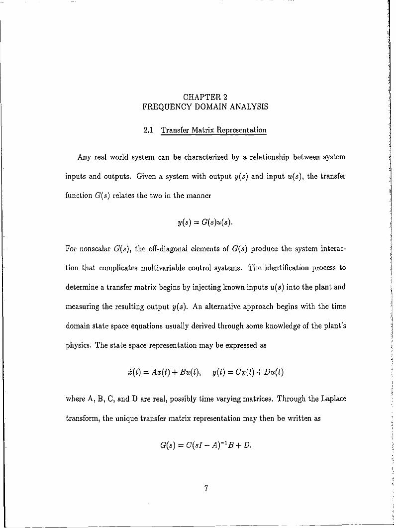
2.1 Transfer Matrix Representation

Any real world system can be characterized by a relationship between system

inputs and outputs. Given a system with output y(s) and input u(s), the transfer

function G(s) relates the two in the manner

y(s) = G(s)u(s).

For nonscalar G(s), the off-diagonal elements of G(s) produce the system interac-

tion that complicates multivariable control systems. The identification process to

determine a transfer matrix begins by injecting known inputs u(s) into the plant and

measuring the resulting output y(s). An alternative approach begins with the time

domain state space equations usually derived through some knowledge of the plant's

physics. The state space representation may be expressed as

=(t) Ax(t) + Bu(t), y(t) = Cx(t) Du(t)

where A, B, C, and D are real, possibly time varying matrices. Through the Laplace

transform, the unique transfer matrix representation may then be written as

G(s) = C(s/ - A)-'B + D.

7

8

B - L/ f dt C

A

Figure 2.1: State Space System Representation.

u(S) G(s) y(S)

Figure 2.2: 'Transfer Matrix System Representation.

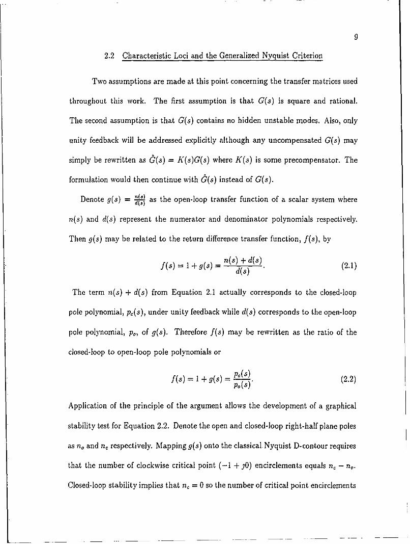
2.2 Characteristic Loci and the Generalized Nyquist Criterion

Two assumptions are made at this point concerning the transfer matrices used

throughout this work. The first assumption is that G(s) is square and rational.

The second assumption is that G(s) contains no hidden unstable modes. Also, only

unity feedback will be addressed explicitly although any uncompensated G(s) may

simply be rewritten as O(s) = K(s)G(s) where K(s) is some precompensator. The

formulation would then continue with a(s) instead of G(s).

Denote g(s) = '(') as the open-loop transfer function of a scalar system where

n(s) and d(s) represent the numerator and denominator polynomials respectively.

Then g(s) may be related to the return difference transfer function, f(s), by

f(s) 1 g(s) = n(s) + d(s)d(s)(2.1)

The term n(s) + d(s) from Equation 2.1 actually corresponds to the closed-loop

pole polynomial, pc(s), under unity feedback while d(s) corresponds to the open-loop

pole polynomial, pa, of g(s). Therefore f(s) may be rewritten as the ratio of the

closed-loop to open-loop pole polynomials or

f~s) = 1 _ g)-pc(s)

AS)=+og(s) (S) (2.2)

Application of the principle of the argument allows the development of a graphical

stability test for Equation 2.2. Denote the open and closed-loop right-half plane poles

as n, and n. respectively. Mapping g(s) onto the classical Nyquist D-contour requires

that the number of clockwise critical point (-1 + 10) encirclements equals nc - no.

Closed-loop stability implies that n, = 0 so the number of critical point encirclements

10

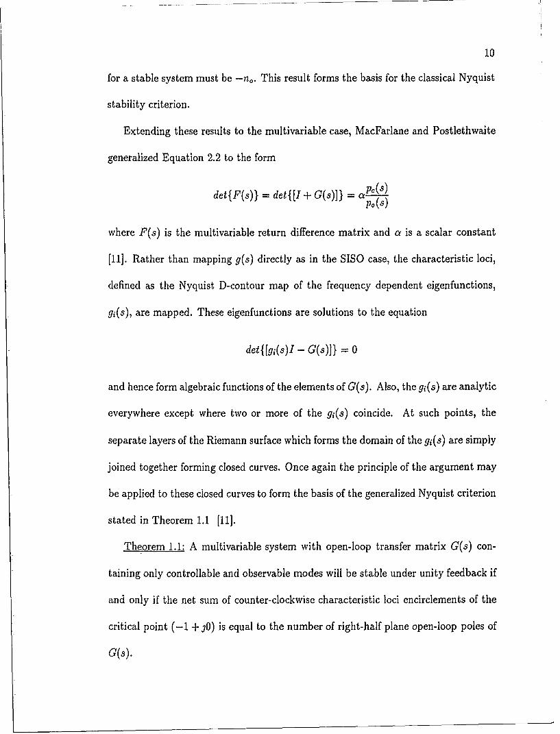
for a stable system must be -n.. This result forms the basis for the classical Nyquist

stability criterion.

Extending these results to the multivariable case, MacFarlane and Postlethwaite

generalized Equation 2.2 to the form

det{F(,s)} = det{E[I + G(s)]} =a -esP0 (S)

where F(s) is the multivariable return difference matrix and a is a scalar constant

[11]. Rather than mapping g(s) directly as in the SISO case, the characteristic loci,

defined as the Nyquist D-contour map of the frequency dependent eigenfunctions,

gj(s), are mapped. These eigenfunctions are solutions to the equation

det{[g,(s)I - G(s)]} = 0

and hence form algebraic functions of the elements of G(s). Also, the gi(s) are analytic

everywhere except where two or more of the gi(s) coincide. At such points, the

separate layers of the Riemann surface which forms the domain of the gi(s) are simply

joined together forming closed curves. Once again the principle of the argument may

be applied to these closed curves to form the basis of the generalized Nyquist criterion

stated in Theorem 1.1 [11].

Theorem 1.1: A multivariable system with open-loop transfer matrix G(s) con-

taining only controllable and observable modes will be stable under unity feedback if

and only if the net sum of counter-clockwise characteristic loci encirclements of the

critical point (-1 + 30) is equal to the number of right-half plane open-loop poles of

G(s).

11

This important theorem allows for a complete graphical stability test of multi-

variable systems in the frequency domain where no model uncertainty is present.

Unfortunately, SISO concepts of system robustness based on gain and phase mar-

gins do not extend to the multivariable case as the eigenfunctions may display large

shifts from relatively small perturbations in the elements of G(s). The next section

addresses the stability of systems in the presence of uncertainties.

2.3 Necessary and Sufficient Stability Conditions

The generalized Nyquist criterion, developed from the characteristic loci method,

provides both necessary and sufficient stability conditions for the nominal plant de-

noted -Go(s) where s = jw on the Nyquist D contour. Stability is guaranteed if and

only if the number of counter-clockwise critical point encirclements by the character-

istic loci equals the number of unstable open loop-poles. Assuming that the nominal

plant itself is stable (either alone or following some type of control implementation),

instability in the perturbed plant, Gp(s), implies a change in the number of critical

point encirclements. If Go(s) and Gp(s) have the same number of of open-loop unsta-

ble poles, then for such a change to occur, at least one eigenvalue of Gp(s) must pass

through the critical point (-1 + jO). Restricting the nominal and perturbed plants

to the same number of open-loop poles requires uncertainty matrix A to be stable

transfer matrix. While this requirement does limit allowable uncertainty structures to

those with no poles in the right-half plane, Foo has shown that unstable perturbations

can generally be decomposed into two stable perturbations allowing the analysis to

continue with a possible increase in conservatism [20].

12

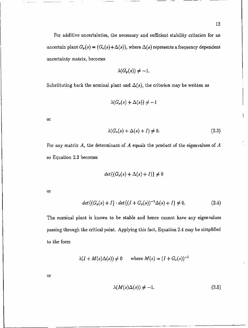
For additive uncertainties, the necessary and sufficient stability criterion for an

uncertain plant Gp (s) = (G, (s) + A (s)), where A(s) represents a frequency dependent

uncertainty matrix, becomes

A(Gp(s)) 5 -1.

Substituting back the nominal plant and A(s), the criterion may be written as

A(Go(s) + A(s)) # -1

or

A(G,(s) + A(s) + 1) # 0. (2.3)

For any matrix A, the determinant of A equals the product of the eigenvalues of A

so Equation 2.3 becomes

det{(G(s) + A(s) + 1)} 0 0

or

det{(Go(s) + I} . det{(I + G(s))-'A(s) + I} 5 0. (2.4)

The nominal plant is known to be stable and hence cannot have any eigenvalues

passing through the critical point. Applying this fact, Equation 2.4 may be simplified

to the form

A(I + M(s)A(s)) 54 0 where M(s) = (I + Go(s)) - '

or

A(M(s)A(s)) # -1. (2.5)

13

Typically, some form of norm bound on either the entire matrix (unstructured uncer-

tainties) or individual elements (structured uncertainties) can be estimated, leaving

the phase information to vary freely. This freedom in choosing the phase of A allows

Equation 2.5 to be written as the necessary and sufficient stability condition

sup p(M(s)A(s)) < 1 (2.6)A(s)

where p denotes the spectral radius. It should be noted that while the preceding

argument addresses additive uncertainties, a similar approach can be appliwd to mul-

tiplicative uncertainties where Gp(s) = Go(s)(I + A(s)). Multiplying on the right by

G,(s) gives

Gp(s) = Go(s) + G.(s)A(s)

or

Gp(s) = Go(s) + A(s) where A(s) = Go(s)A(s).

Although Equation 2.6 provides necessary and sufficient stability conditions for

uncertain systems, it is quite difficult to compute because the entire range of A must

be considered. Furthermore, the solution lacks convexity allowing for the possibility

of multiple maxima. This unfortunate situation greatly complicates attempts to find

the true supremum of p(M(s)A(s)) over A(s). Because of the difficulties involved

in solving Equation 2.6, singular value techniques were developed to provide upper

bounds on permissible model uncertainties. Before introducing these techniques, a

mathematical description of several important uncertainty classes will be presented.

14

2.4 Uncertainty Classes

So far, the frequency dependent uncertainty matrix, A(s), has been used to

represent the additive or multiplicative uncertainty present in control system. No in-

formation has been provided on the structure of A(s) which turns out to be quite im-

portant in the actual mathematical analysis of system stability. Rather than propos-

ing one all-encompassing model for A(s) to account for system uncertainty, three

representations will be presented with varying degrees of information required for

each one. In developing these three models, two main objectives are observed:

1. The model should handle all information available concerning the system's ac-

tual uncertainties. All impossible uncertainty structures should be excluded to

reduce conservatism of the stability analysis.

2. The model should be as simple as possible so that the analysis process is not

unnecessarily complex. Simplified models also encourage an interactive design

process so various control designs may be quickly generated and compared.

Naturally, these objectives produce conflicting requirements and careful consideration

must be used to select an appropriate model. In any event, a conservative stability

analysis is preferable over one that is simple but erroneous.

The three uncertainty models considered here include unstructured uncertainties,

element- by-element structured uncertainties, and block diagonal structured uncer-

tainties. In each of these classes, the uncertainty matrix A(s) is complex with sk'.ne

form of norm bound placed on the magnitude of the matrix or matrix elements. The

15

simplest uncertainty class to describe and manipulate concerns unstructured uncer-

tainties which may be mathematically represented as

DU {A I 1A112 < 6 E W}

where 1. l[ represents the standard matrix 2-norm and 5 a real scalar. (Here, and

in the remainder of this work, frequency dependence will be implied). From the

definition, it is apparent that no information concerning the inner structure of A is

accessible. This effectively places a SISO bound on a MIMO system greatly hinder-

ing efforts to reduce conservatism if information about the inner structure of A is

available.

The second uncertainty class, element-by-element structured uncertainties, pro-

vides a rich source of information about A. This class is defined as

D3 {A = {6ij} I 16ji 5 Pij E R+}

where a magnitude bound is placed on each element of uncertainty matrix A allowing

information on the inner structure of A to remain a part of the stability analysis

process. Class D, provides a more realistic representation of real world uncertainty

than that of the unstructured uncertainty class.

To illustrate the advantages of structured uncertainties over unstructured uncer-

tainties, consider some process plant with two independent control valves whose flow

rate is known within ±10% [21]. As a structured uncertainty, A could be correctly

represented as51 0

I= 16d < 0.1.0 52

16

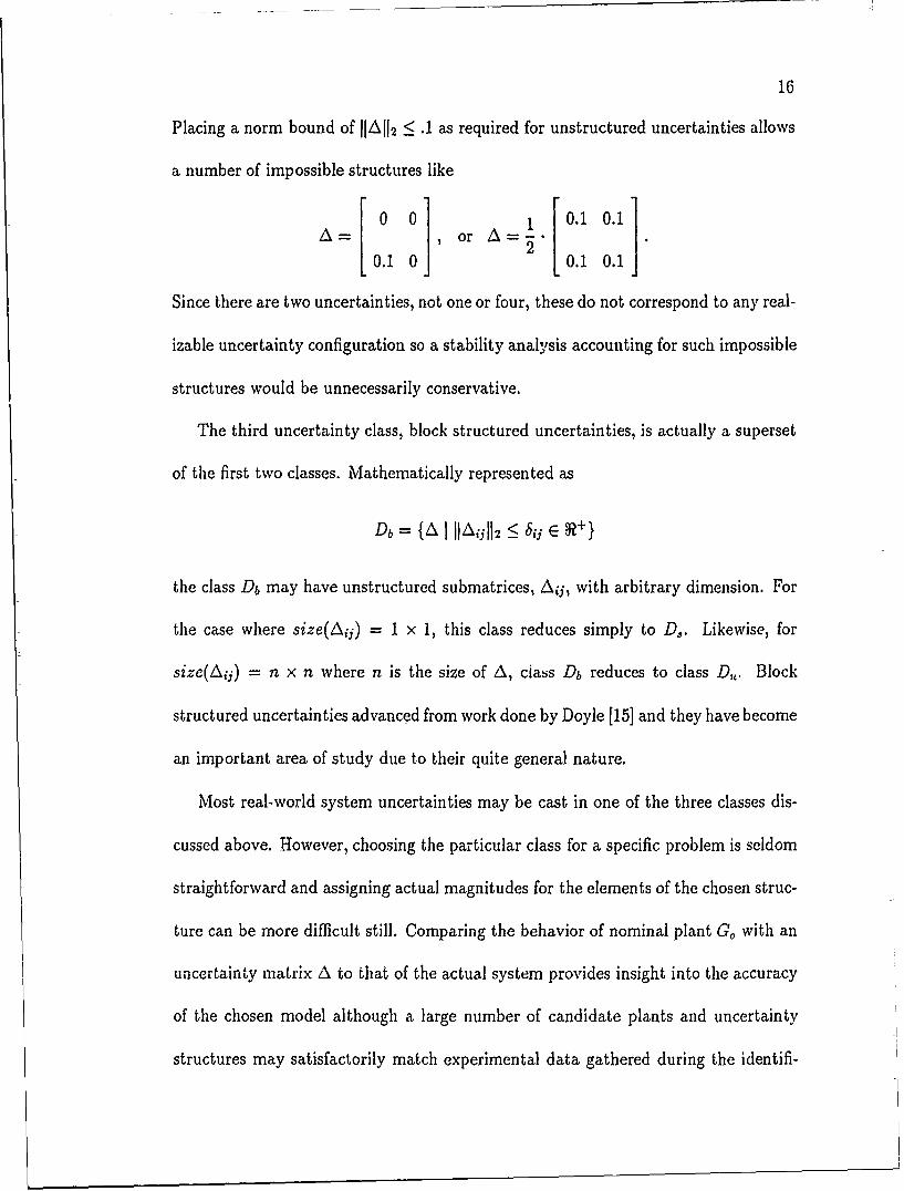
Placing a norm bound of IJAI[2 < .1 as required for unstructured uncertainties allows

a number of impossible structures like

0 0 i 0.1 0.1A= or A=-..

0.1 0 0.1 0.1

Since there are two uncertainties, not one or four, these do not correspond to any real-

izable uncertainty configuration so a stability analysis accounting for such impossible

structures would be unnecessarily conservative.

The third uncertainty class, block structured uncertainties, is actually a superset

of the first two classes. Mathematically represented as

A = {A I [[AiI2 < bij E R+}

the class D6 may have unstructured submatrices, Aij, with arbitrary dimension. For

the case where size(Ait) = 1 x 1, this class reduces simply to D,. Likewise, for

size(Aft) = n x n where n is the size of A, ciass Db reduces to class D,. Block

structured uncertainties advanced from work done by Doyle [15] and they have become

an important area of study due to their quite general nature.

Most real-world system uncertainties may be cast in one of the three classes dis-

cussed above. However, choosing the particular class for a specific problem is seldom

straightforward and assigning actual magnitudes for the elements of the chosen struc-

ture can be more difficult still. Comparing the behavior of nominal plant G, with an

uncertainty matrix A to that of the actual system provides insight into the accuracy

of the chosen model although a large number of candidate plants and uncertainty

structures may satisfactorily match experimental data gathered during the identifi-

17

cation process. Narrowing down which of these candidate model combinations best

approximates the actual system becomes a process of model invalidation as those

models that fail to satisfy some matching criteria are eliminated. No discussion of

how a designer should choose one model over another will be presented here since

this is a complete field unto itself. However, a description of the problem by Smith

and Doyle may be found in [22].

While most real-world systems may be characterized by one or more of the uncer-

tainty classes described here, it must be noted that other models offering improved

model agreement exist for some specific problems. Most notable of these other mod-

els are those that deal with combinations of both- real and complex uncerbainties and

those that address repeated or dependent uncertainty structures. In the three uncer-

tainty structures discussed above, unstructured, element-by-element structured, and

general block structured, some form of bound was placed on the magnitude of the

uncertainty. Such magnitude bounds allow the phases of the uncertainty elements

or blocks to vary freely between 0 and 21r so that worst case situations can be ad-

dressed. For many uncertainty sources like unmodelled dynamics, this phase freedom

is mandatory to establish necessary and sufficient stability conditions. However, if

some or all elements of an uncertainty structure are known to be strictly real, this al-

lowable phase variation may provide for an overly conservative stability analysis [23].

A method for treating strictly real uncertainties was proposed by De Gaston and

Safonov [24]. This method transforms the perturbed plant Gp into a series of convex

hulls in the complex plane and, through an iterative process, determines a stabil-

18

ity margin that indicates the largest scalar multiplier of A for which stability is

guaranteed. This approach provides necessary and sufficient stability conditions but

only if an infinite number of iterations are performed. Fortunately, usable results

are generally obtained for a finite number of iterations though the method is still

computationally intensive.

For uncertainties consisting of combinations of real and complex elements, alter-

native formulations of the structured singular value have been proposed by several

authors [23, 25, 26]. While these approaches appear to reduce the conservatism over

methods that consider only complex uncertainty structures, a number of theoretical

and computational challenges must be resolved before they can be reliably applied to

engineering problems.

In addition to special uncertainty models addressing real elements, the case of

repeated or dependent complex uncertainty models requires special consideration.

This class is actually a subset of the other structured uncertainty classes with the

distinction that two or more-of the elements or blocks of A are constrained such that

their pha.ses must always be the same [27]. Thus, while the phases may vary between

0 and 27r, they may not. do so independently of one another.

While the real and repeated uncertainty element models provide an improved

stability analysis for their particular cases, the two structured uncertainty classes

presented earlier account for a wide range of important problems. Therefore, only

their treatment will be considered in the remainder of this work.

CHAPTER 3SINGULAR VALUE TECHNIQUES

3.1 The Singular Value Decomposition

As discussed in Section 2.3, the necessary and sufficient stability criterion

sup p(MA) < 1 (3.1)A

is nonconvex making it difficult if not impossible to determine the range of permissi-

ble As. Rather than giving up on this approach for uncertain multivariable systems,

it is possible to continue the analysis using relationships involving the singular value

decomposition. These relationships start out as conservative upper bounds but the

results of Chapter 4 show that this conservatism can generally be eliminated com-

pletely. The singular value decomposition is defined for any matrix A E C ×"x as

A = XrYH (3.2)

where X and Y are unitary matrices the columns of which form the left and right

singular vectors of A respectively. The diagonal matrix E contains the singular values

of A in decreasing order of magnitude. The singular values and vectors of A can be

determined in terms of the eigenvalues and eigenvectors of the hermetian forms A"A

and AA H as

AHAY = o'?Yi

AA HX, = 0?X,. (3.3)

19

20

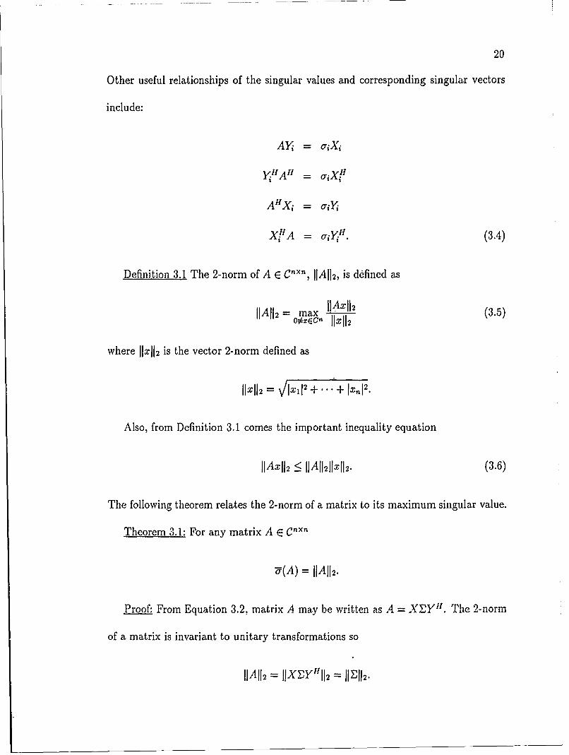
Other useful relationships of the singular values and corresponding singular vectors

include:

AY = oiXj

yiHAH = oiX 1

AHX = o'i Y

XjHA =oi . (3.4)

Definition 3.1 The 2-norm of A E Cn ×" , IIAlt 2, is defined as

IIAi 2 = m IIAxl2 (3.5)o, - 11x112

where 11X112 is the vector 2-norm defined as

I1IX12 = j112 +... + IXn12.

Also, from Definition 3.1 comes the important inequality equation

jjAxII2 5 <IAIl21lxlI2. (3.6)

The following theorem relates the 2-norm of a matrix to its maximum singular value.

Theorem 3.1: For any matrix A E Cn x n

5(A) = IIA1j 2.

Proof: From Equation 3.2. matrix A may be written as A = XEY1". The 2-norm

of a matrix is invariant to unitary transformations so

IIAllk = IIXIY"I12 = II 1h12

21

From Definition 3.1, this may be written as

_____l iu~il2 +"". + O 1 -I2IIAI1 = lFII12 = max = max

0OXEoo 11x112 Oi-ECn l/i112 + ... + JX,42

Choosing x = el, the first standard basis vector gives EX 2 = Orl(A) while any other

choice for x gives IEX2 < Or,(A). Therefore, IhAil 2 = ri(A) -"(A). s

E11-12-

Using this result, the following lemma relates 7(A) to p(A).

Lemma 3.1 For any matrices A, B E Cn× ,,

p(AB) :_ "d(AB). (3.7)

Proof: From the eigenvalue/eigenvector equation we have

ABW4 = AX.

where Ai is an eigenvalue of (AB) and Wi the corresponding eigenvector. Taking the

2-norm of both sides gives

[[ABWV[[2 = [[Ai [[i = [AI[[[WiI2.

Equation 3.6 allows this to be written as an inequality

IIABII 21IW II2 > IIABWdII 2 = IAIIIWII2.

Applying Theorem 3.1 along with the definition of the spectral radius gives

-Y(AB) >_ p(AB). a

Finally, the 2-norm of a matrix product is related to the product of the 2-norms

as shown in the following lemma.

22

Lemma 3.2 For A, B E Cnx n

" (AB) _ "(A)'(B). (3.8)

Proof: Again, from Definition 3.1

IIABII 2 = max IIABxII 2 < max IIAIkII2IA112 m IIBxD2O X n X11 l 2 7- E 1 1 -T I 1 2 O 4 E n I X 1

or

lIABI 2 _< IIAII2iBI2.

Replacing A and B with M and A respectively in Equations 3.7 and 3.8, the following

expression must hold:

p(MAX) <5 -(MA) <5 -(M)U(AX).

From these relationships, the necessary and sufficient stability criterion of Equation

3.1 can be written as the following sufficient stability conditions

supU(A'I)5(A) < 1 (3.9)A

and

sup (MA) < 1. (3.10)

A

Since Equations 3.9 and 3.10 only guarantee sufficient stability conditions for

structured uncertainties, additional manipulations are required to reduce conser-

vatism with the intent of regaining the necessary stability condition. Two techniques

that address this problem are nonsimilarity scaling introduced by Kouvaritakis and

Latchman [161 and similarity scaling advanced by Doyle [15]. Both techniques rely

on the fact that while the eigenvalues (and hence the spectral radius) of a matrix are

unaffected by similarity transformations, the singular values are not necessarily

23

preserved atnd may, in fact, be reduced. The nonsimilarity scaling technique will be

discussed first with the analysis limited to element by element bounded uncertainties.

3.2 Structured Uncertainties with Nonsimilarity Scaling

The nonsimilarity scaling formulation starts with the necessary and sufficient

stability criterion of Equation 3.1. Introducing positive, diagonal matrices R and L

to this expression gives the equivalent stability condition

sup p(MA) = sup p(R-'ML-'LAR) < 1.A AX,

This may be rewritten in the form of Equation 3.9 giving the sufficient stability

criterion

sup (R-1 ML- 1) (LAR) < 1. (3.11)A

Equation 3.11 no longer conforms to the similarity transformation structure: hence

the name "nonsimilarity scaling." However, the free elements of R and L still allow

the conservatism gap between the maximum singular value upper bound and the

spectral radius lower bound to be reduced. Also, the choice of positive values for

the elements of R and L allows a simplification based on the following lemmas and

Theorem 3.2.

Lemma 3.3: For all A E Cn×"n and B E Rn×n where bij 0 and ajI < bij for all

ij, with x+ defined as (Ixil,..., IXnl)T,

JjAxJJ2 < i]Bx+11 for all x E Cn. (3.12)

24

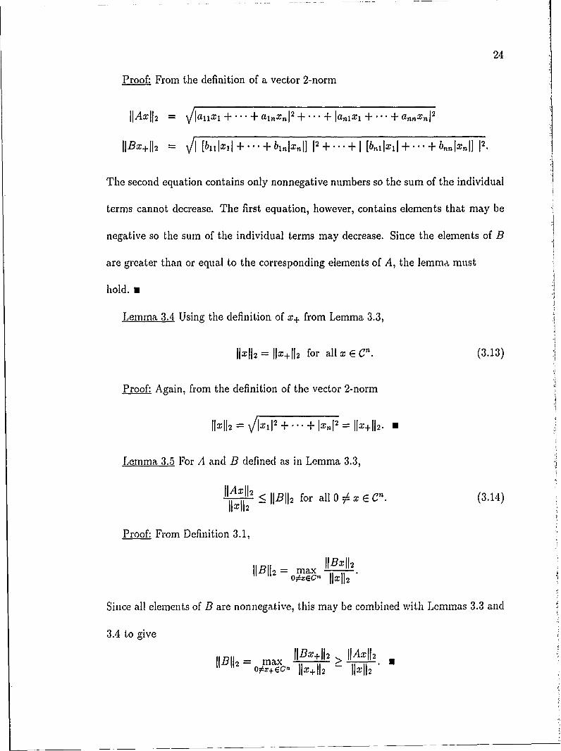
Proof. From the definition of a vector 2-norm

IlAxI[ 2 = VIallx, + ... + aInXnI 2 + ... + Ianixi + + a2nnxn 12

IBx+112 = VI [bijxjj + -.. -+ blnlxnl] 2 +... + I [b,ixjj + -...+ bnlxnI] 12.

The second equation contains only nonnegative numbers so the sum of the individual

terms cannot dccrease. The first equation, however, contains elements that may be

negative so the sum of the individual terms may decrease. Since the elements of B

are greater than or equal to the corresponding elements of A, the lemm, must

hold. n

Lemma 3.4 Using the definition of x+ from Lemma 3.3,

IxII12 IIx+1Ib for all x E C. (3.13)

Proof: Again, from the definition of the vector 2-norm

IxI11 - Jx1 ' ... + Jx, 2 - IIx+112. *

Lemma 3.5 For A and B defined as in Lemma 3.3,

IAxII2 < JIBI12 for all 0 # x E C. (3.14)

114U2

Proof: From Definition 3.1,

IIBxII2IIBI12 -max

Since all elements of B are nonnegative, this may be combined with Lcmmas 3.3 and

3.4 to give

11B1 2 = ma h > I

T~+112 If11

25

Theorem 3.2: Given A E Cn ×n , positive, diagonal matrices L, R E Rnxn and

P E Rnxn where Pij - 0 and 8i6i _ pli for all i,j,

-(LAR) < -(LPR). (3.15)

Proof: This proof follows directly from Lemmas 3.3, 3.4, and 3.5 with A replaced

by LAR and B replaced by LPR so that

o IAX112 ffLPRx+112JILAR112 = max < max ."LPURI12. 0oOXEoo I1X1 2 - o0x+EC ilX+Ill

Theorem 3.2 and the definition of element-by-element structured uncertainties

from Section 2.4 allow the direct substitution of P for A in Equation 3.11.

Substituting P for A would appear to add additional conservatism to Equation

3.11. However, Lemma 3.6 shows that this is not the case.

Lemma 3.6 Given LAR and LPR defined as in Theorem 3.2, the following equality

must hold:

sup 7(LAR) = "j(LPR). (3.16)A

Proof: The freedom of the phases of each element of A allows 6ij - ij -- Pij

for all i,j. Therefore, by individually adjusting the phases of each element of A, the

equality of Equation 3.16 is established. n

Since P always represents a realizable variation of A, there is actually no added

conservatism by substituting P for A. Therefore the sufficient stability condition of

Equation 3.11 becomes

inf'U(R-'ML-I)'5(LPR) < 1 (3.17)L,R

26

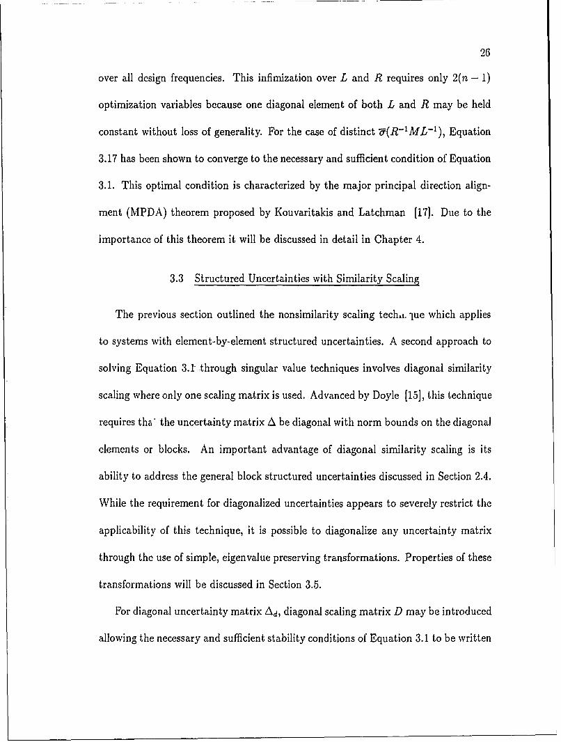
over all design frequencies. This infirization over L and R requires only 2(n - 1)

optimization variables because one diagonal element of both L and R may be held

constant without loss of generality. For the case of distinct "U(R-'ML-1 ), Equation

3.17 has been shown to converge to the necessary and sufficient condition of Equation

3.1. This optimal condition is characterized by the major principal direction align-

ment (MPDA) theorem proposed by Kouvaritakis and Latchman [17). Due to the

importance of this theorem it will be discussed in detail in Chapter 4.

3.3 Structured Uncertainties with Similarity Scaling

The previous section outlined the nonsimilarity scaling techi. que which applies

to systems with element-by-element structured uncertainties. A second approach to

solving Equation 3.1 through singular value techniques involves diagonal similarity

scaling where only one scaling matrix is used. Advanced by Doyle [15], this technique

requires tha' the uncertainty matrix A be diagonal with norm bounds on the diagonal

elements or blocks. An important advantage of diagonal similarity scaling is its

ability to address the general block structured uncertainties discussed in Section 2.4.

While the requirement for diagonalized uncertainties appears to severely restrict the

applicability of this technique, it is possible to diagonalize any uncertainty matrix

through the use of simple, eigenvalue preserving transformations. Properties of these

transformations will be discussed in Section 3.5.

For diagonal uncertainty matrix Ad, diagonal scaling matrix D may be introduced

allowing the necessary and sufficient stability conditions of Equation 3.1 to be written

27

as

sup p(MAd) = sup p(DMAdD -1 ) < 1 (3.18)Ad Ad

and the sufficient condition of Equation 3.10 as

sUP'&(DMAdD- 1) < 1. (3.19)Ad

Taking advantage of the diagonal nature of Ad permits a decomposition of the form

Ad= PdUd

where Pd, > I6d, I for all i and Ud is a diagonal unitary matrix. This allows Pd to

retain the magnitude information and Ud the phase information of Ad. Substituting

PdUd for Ad in Equation 3.19 gives the sufficient stability condition

sup p(MA,:) < sup"(DMPdUdD-1 ) < 1.Ad Ud

Noting that diagonal matrices commute with each other, the positions of Ud and D - '

may be exchanged making the condition

sup p(MAd) <_ sup-5(DMPdD'Ud) < 1. (3.20)Ad Ud

However, the 2-norm, and hence the maximum singular value, of a matrix is invariant

to unitary transformations removing the dependence on Ud. Combining M and Pd

into M = MPd, the condition of Equation 3.20 becomes

sup p(MAd) _< inf -(DMaD-')< 1. (3.21)Ad

Since the spectral radius of MUd is always bounded from above by the maximum

singular value of DMaD - 1, the free elements of D may be used to reduce the conser-

vatism gap between the maximum singular value upper bound and the spectral radius

28

lower bound of Equation 3.21. For the general case where a stationary point occurs

at the "inf," the resulting optimal value of W(DMaD - 1) is known as the "structured

singular value" of Ma (denoted t(Ma)).

The original definition of the structured singular value had the form [151

0 if no A solves det{[I + MA]} =0 }else (minA {(A) I det{(I + MA]} = 0}) -1

While this expression is rather unwieldy, a more useful alternative formulation is given

by

i(Ma) = sup p(M.Ud) <_ inf'e(DMaD-1). (3.22)Ud D

The right-hand side of Equation 3.22 has been proven convex (with respect to scaling

matrix eD) [28, 29] and the MPDA formulation for similarity scaling shows that the

inequality becomes an equality at the "inf" for stationary points of'p(DM -'D1 ) [17].

Chapter 4 reviews conditions required for the optimal solution to Equation 3.22.

However, an interesting suboptimal solution was proposed by Safonov involving the

Frobenius norm minimization of DMD -1 [141. Since the Frobenius norm of a

matrix provides an upper bound on the 2-norm (and hence the maximum singular

value) of the matrix, reducing the Frobenius norm. of DMD -1 generally serves to

reduce "e(DMaD- 1) as well. An iterative algorithm introduced by Osborne performs

such a reduction by choosing elements of D that equalize the row and column sums of

DMVD -I [30]. While this procedure produces a conservative upper bound for /(Ma,),

it is numerically inexpensive since no singular value decompositions are required.

29

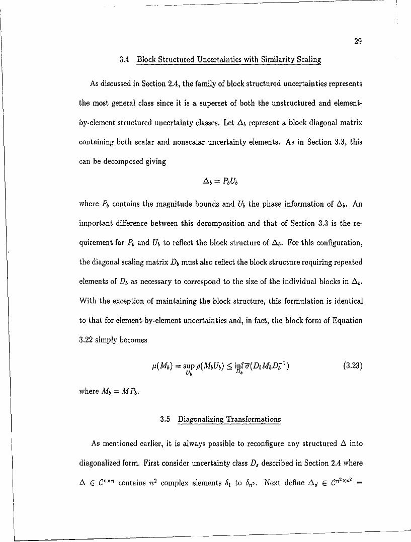
3.4 Block Structured Uncertainties with Similarity Scaling

As discussed in Section 2.4, the family of block structured uncertainties represents

the most general class since it is a superset of both the unstructured and element-

by-element structured uncertainty classes. Let Ab represent a block diagonal matrix

containing both scalar and nonscalar uncertainty elements. As in Section 3.3, this

can be decomposed giving

Ab = PbUb

where Pb contains the magnitude bounds and Ub the phase information of Ab. An

important difference between this decomposition and that of Section 3.3 is the re-

quirement for P and Ub to reflect the block structure of Ab. For this configuration,

the diagonal scaling matrix Db must also reflect the block structure requiring repeated

elements of Db as necessary to correspond to the size of the individual blocks in Ab.

With the exception of maintaining the block structure, this formulation is identical

to that for element-by-element uncertainties and, in fact, the block form of Equation

3.22 simply becomes

y(Mb) = sup p(MbUb) < inf -(DbMbD' 1 ) (3.23)Ub Db

where Mb = MPb.

3.5 Diagonalizing Transformations

As mentioned earlier, it is always possible to reconfigure any structured A into

diagonalized form. First consider uncertainty class D, described in Section 2.4 where

A E Cn ×" contains n2 complex elements 81 to &2. Next define Ad E Cn2 ×n2

30

diag[61,..., &,2]. It is always possible to relate Ad to A using transformation matrices

E1 E Rxn,2 and E2 E Rn2xn containing only l's and 0's such that ElAdE 2 = A. From

this relationship, the necessary and sufficient stability conditions of Equation 3.1 may

be written as

sup p(MEAdE2 ) < 1.Ad

At this point, some means of recovering the simplifying properties of diagonal matrices

required by Equation 3.20 is needed. The following theorem relates the eigenvalues

(and hence the spectral radius) of matrix products (AB) and (BA).

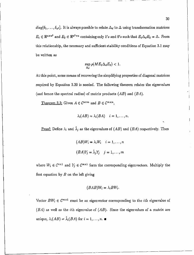
Theorem 3.3: Given A E Cn " and B E Cmxn,

A (AB) = Ai(BA) i = 1,... ,n.

Proof: Define Ai and Aj as the eigenvalues of (AB) and (BA) respectively. Then

(AB)W =Aj W i= 1,...,n

(BA)Yj = AjY j =1.,rn

where Wi E CnX' and Yj E Cmxl form the corresponding eigenvectors. Multiply the

first equation by B on the left giving

(BAB)Wj = A BW .

Vector BWi E Cmxl must be an eigenvector corresponding to the ith eigenvalue of

(BA) as well as the ith eigenvalue of (AB). Since the eigenvalues of a matrix are

unique, )q(AB) = Ai(BA) for i = 1,...,n. n

31

Using this result, replace A by MEPd and B by E2 so the spectral radius equa-

tions become

p(MA) = p(E 2MEIAd).

Next, define M,, = E2 ME1 and the necessary and sufficient stability condition of

Equation 3.1 may be written

sup p(MaAd) < 1.Ad

Starting at this point, the analysis of Section 3.3 can then continue as before.

While this diagonalizing transformation is straightforward, it has the unfortunate

consequence of increasing the system size from n x n to as much as n' x n" with a

resultant increase in computational requirements to compute the maximum singular

values. Also, the number of optimization variables required to infimize Equation 3.22

can increase to n2 - 1 versus 2(n - 1) for nonsimilarity scaling. (As with matrices L

and R of Equation 3.17, a single element of D may be arbitrarily fixed allowing the

elimination of one optimization variable). Even with these disadvantages, the ability

to manage block structured uncertainties makes similarity scaling an invaluable tool

in the analysis of uncertain systems.

CHAPTER 4

THE MAJOR PRINCIPAL DIRECTION ALIGNMENT PROPERTY

4.1 Application to Sinlarity Scalin

The use of singular value techniques in the form of nonsimilarity and similarity

scaling has the disadvantage of initially reducing the necessary and sufficient stabil-

ity conditions of Equation 3.1 to simply sufficient conditions. For convenience, the

relevant equations zre repeated.

sup'(MA) " inf-(R-1AiL-1 )(LPR) Nonsimilarity Scaling (4.1)

"% - L,R

sup p(MA) < inf-(DMaD- ) Similarity Scaling. (4.2)a -D

Eliminating con3ervatism in these singular value formulations requires establishing

conditions for which the inequalities hold with equality. This section reveals that

acbieving equality in Equations 4.1 and 4.2 is simply a matter of invoking the MPDA

property [17]. Although MPDA conditions have been shown to exist for both non-

similarity and similarity formulations, this discussion will focus only the similarity

scaling techniques.

Definition 4.1: The major right principal direction, Y1, and the major left prin-

cipal direction, X1, of matrix A are the right and left singular vectors of matrix A

corresponding to U(A).

32

33

Theorem 4.1: For any matrix A E Cn x n

p(A) ='F(A)

if and only if X 1 and Y are aligned within a scaling factor el0 such that

Y = e0X1. (4.3)

Proof: For notational simplicity, denote "(A) by - and p(A) by p. Vectors X1 and

Y from the singular value decomposition must be unique with respect to one another

within a scaling factor e0 . Multiplying both sides of Equation 4.3 on the left by A

gives

AY1 = eJ°AX 1.

Also, the relationships of Section 3.1 show that AY1 = dX1 so this can be rewritten

as

AX 1 = "5e-)°XI

indicating that ae-JO actually corresponds to an eigenvalue of A. Since eigenvalues

of a matrix are always magnitude bounded by the maximum singular value of the

matrix, sufficiency of the theorem is established.

Establishing the necessity of the theorem starts with the assumption that U = p

so some eigenvector Z1 exists where

AZI = e'-UZ1 (4.4)

and

ZH-A = -C&'Zf. (4.5)

34

Multiplying Equation 4.4 on the left by Equation 4.5 and noting the AHA = Y 2 Y

provides the following expression:

Z(HAHAZI _ ZHYE2YHZ 1 -2ZH ZI ZfIYYHZ 1

This may be simplified by defining a new vector W1 = YIHZ 1 to give

W IH E2W1 =. 72. (4.6)

WH W,

Equation 4.6 can only be satisfied if W = eJ ej where el is the first standard basis

vector. Therefore, Z1 = YW 1 = eJOYel = eJOY 1. Substituting back into Equation 4.4

then gives

Ael1 = vVOX, = elC-Oy,

or

X, = eJPY

establishing the necessity of the theorem. n

Corollary 4.1: For the case of repeated singular values of A E Cnxn where q denotes

the multiplicity of o,

p(d) = al (A),. . ., q (A)

if and only if the subspaces spanned by X 1,..., Xq and Y1,..., Y are aligned within

a scaling factor e0.

Proof: From Equation 3.2 the singular vectors of matrix A with a repeated maxi-

35

mum singular value are defined as

AHAY 1 = o Y1 AAHX 1 Iu'X1

and

AHAYq= I' Yj AAHXq = IrXq

Therefore, linear combinations of the first q columns of X or Y form legitimate

solutions for X1 and Y1 respectively. Combining these solutions with Theorem 4.1

completes the proof. n

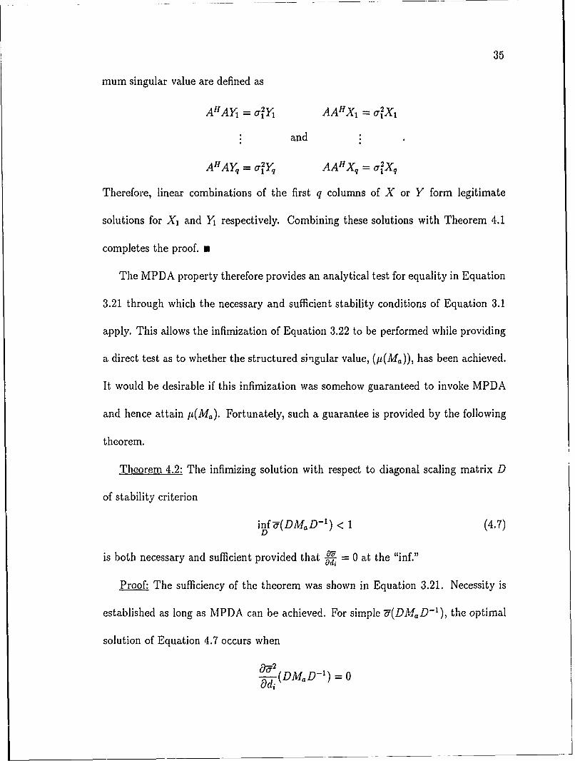
The MPDA property therefore provides an analytical test for equality in Equation

3.21 through which the necessary and sufficient stability conditions of Equation 3.1

apply. This allows the infimization of Equation 3.22 to be performed while providing

a direct test as to whether the structured singular value, (ii(Ma)), has been achieved.

It would be desirable if this infimization was somehow guaranteed to invoke MPDA

and hence attain p(Ma). Fortunately, such a guarantee is provided by the following

theorem.

Theorem 4.2: The infimizing solution with respect to diagonal scaling matrix D

of stability criterion

inf'7(DM,,D- ') < 1 (4.7)D

is both necessary and sufficient provided that 0 at the "inf."

Proof: The sufficiency of the theorem was shown in Equation 3.21. Necessity is

established as long as MPDA can be achieved. For simple "5(DA'aD- ), the optimal

solution of Equation 4.7 occurs when

-(DM,,D 1 ) = 0Oai

36

indicating a stationary point. As mentioned in Section 3.3, the left-hand side of

Equation 4.7 is convex with respect to scaling matrix eD so any local minimum is the

global minimum. Therefore the only stationary point must correspond to the optimal

solution. By direct differentiation, the stationarity condition becomes

- = 2Y [IIfE Ia 2E] Y =0 (4.8)

where M fa = DMA D-, and Ei is a square matrix containing a "1" in the iith position

and "Os" elsewhere. (Note: the actual differentiation is omitted here but the complete

differentiation of a similar function appears ;n Section 5.5).

Examining conditions at which Equation 4.8 equals zero reveals the requirement

that

lxiii = lyd i = 1,...,n (4.9)

which is in fact the MPDA requirement that the magnitudes of the elements of X

and Y1 be equal.

Completion of the proof from this point requires that some Ud exists such that

the phase alignment of X1 and Y occurs. The existence of such a Ud then guarantees

that p(MUd) = "5(DMaD-Ud) = f(Ma). From the singular value decomposition,

the principal singular vectors are related as

(DM.D-1)Y = " Xl

Xf(DMaD- ') = YH.

Introducing a diagonal unitary matrix, Ud, allows these equations to be rewritten as

37

(DMaD-'Ud)UdHY = -Xl

X1(DM.D-Ud) = -'YIHUd. (4.10)

From Equation 4.10 it is apparent that the diagonal elements of Ud may be used to

alter the phases of X, and Y while continuing to satisfy the MPDA requirement that

the magnitudes of the corresponding elements of X1 and Y be equal. The ability to

achieve independent phase alignment of X1 and Y1 by Ud completes the proof. n

The result of this theorem is that optimization of Equation 4.7 has the effect

of directly invoking MPDA at the "inf" for simple U, guaranteeing the necessary

and sufficient stability conditions. Cases with nonsimple U (known as "cusps") do

not necessarily contain a stationary point at the "inf" and must be analyzed using

different techniques. A more complete discussion of cusping systems appears in

Chapter 8.

4.2 Block Structured Uncertainties

By following the MPDA development for scalar uncertainties, a similar formu-

lation results for general block structured uncertainties. The main difference is the

requirement of maintaining the individual block structures rather than considering

each element of A individually. As discussed in Section 3.4, this block structure must

be reflected in the scaling matrices as well. The optimal solution is then characterized

by the equalization of the 2-norms in the corresponding blocks of the left and right

principal vectors X1, and Y1 respectively. The same guarantee of achieving equality

38

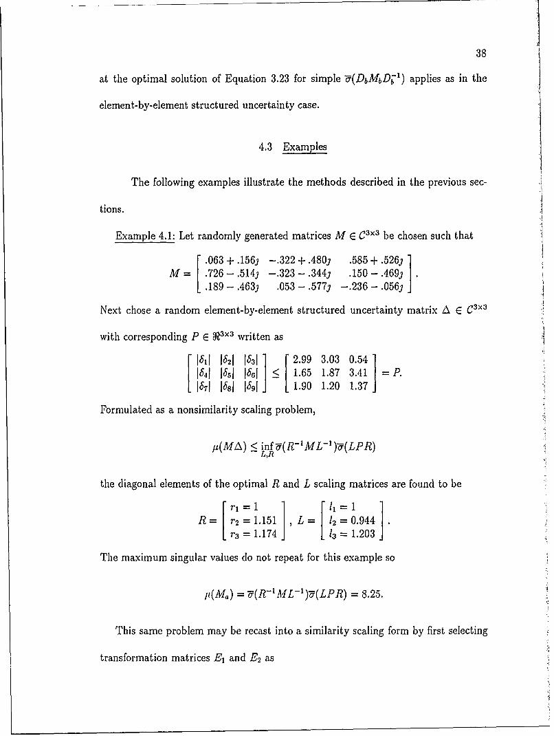
at the optimal solution of Equation 3.23 for simple U(DbMbDb1) applies as in the

element-by-element structured uncertainty case.

4.3 Examples

The following examples illustrate the methods described in the previous sec-J

tions.

Example 4.1: Let randomly generated matrices M E C3x3 be chosen such that

.063 + .1561 -. 322 + .4801 .585 + .5261M= .726 - .5141 -.323- .3443 .150-.4693

.189- .4631 .053 - .5771 -.236 - .0561

Next chose a random element-by-element structured uncertainty matrix A E C3X3

with corresponding P E × written as

1611 1821 1831 2.99 3.03 0.54 J1841 1851 1861 < 1.65 1.87 3.41 --P.1871 1881 1691 1.90 1.20 1.37

Formulated as a nonsimilarity scaling problem,

p(MA) < inf'd(R-'ML-)'(LPR)

L,R

the diagonal elements of the optimal R and L scaling matrices are found to be

rl r=1 11[41 1R= r 2 =1.151 ,L= 12=0.944

r3 = 1.174 13 = 1.203

The maximum singular values do not repeat for this example so

/t(Ma) = ?(R-1 .L-' ) (LPR) = 8.25.

This same problem may be recast into a similarity scaling form by first selecting

transformation matrices E, and E 2 as

39

1 00010

0 0 111 1 0 0 0 0 0 01 10 0

E= 0 0 0 1 1 1 0 0 0 E2 0 1 00 00000 1 1 00 1

100

01 0L0 0 1J

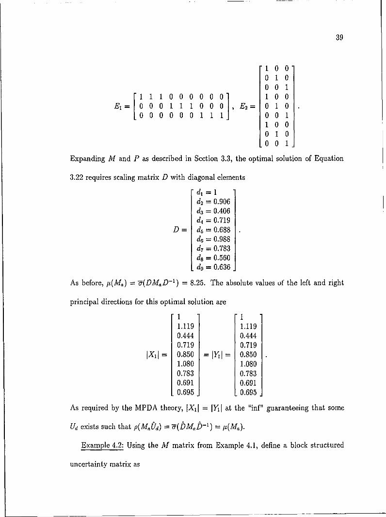
Expanding M and P as described in Section 3.3, the optimal solution of Equation

3.22 requires scaling matrix D with diagonal elements

d = 1d2 = 0.906d3 = 0.406d4 = 0.719

D= d5 =0.688d6 = 0.988d7 = 0.783d8 = 0.560d9 = 0.636

As before, y(Ma) = -5(DMfD - 1) = 8.25. The absolute values of the left and right

principal directions for this optimal solution are

1 11.119 1.1190.444 0.4440.719 0.719

IXi = 0.850 = Y, I= 0.8501.080 1.0800.783 0.7830.691 0.6910.695 0.695

As required by the MPDA theory, 1X11 = Y I at the "inf" guaranteeing that some

Ud exists such that p(Ma]d) = "(bM b - ) = i(Ma).

Example 4.2: Using the M matrix from Example 4.1, define a block structured

uncertainty matrix as

40

Si 62 63L= 64

6.5 Ab

where 61 through 65 are scalar uncertainties such that 16i] _< pi and A, is a 2 x 2 block

with 5(Ab) < Pb. Block Ab may be represented as

Ab = PbUb

where Pb is a 2 x 2 matrix with j(Pb) = pb and Ub is a 2 x 2 unitary matrix containing

the phase information of Ab. We may now define a matrix P& containing randomly

generated bounds on the 6i and Ab elements as

2.99 3.03 0.54

P,, 1.651.90 P J

with 5(Pb) = 1.87. It is easily shown that the worst case structure for Pb in terms of

1 (Mb) occurs when

P 6 [l.0 1.87

allowing a P matrix for this case to be written as

2.99 3.03 0.54P 1.65 1.87 0

1.90 0 1.87

The 2 x 2 block structure constrains the last two terms of scaling matrix Db to be

identical thus eliminating one degree of freedom from the optimization. Also, the two

zero elements of P allow the diagonalized matrix Pd (and hence lb) to be of size

7 x 7 rather than 9 x 9.

Choose

41

100010

1110000 001

El---00001010 E2 100000 10 1]E0 100

010001

corresponding to Pd = diag[2.99, 3.03, 0.54, 1.65, 1.9, 1.87, 1.87] so that P -

EPdE2. Expanded matrix Mb may then be formed as Mb = E2MEPd. Following

the infimization of "(DbMbDb'), the optimizing Db and the absolute values of the

elements of X1 and Y' are found to be

di = 1 0.427 0.427d2 = 0.82 0.527 0.527d3 = 0.41 0.187 0.187

Db = = 0.63 lXII= 0.269 , 1Y1= 0.269d5 = 0.87 0.373 0.373d6 = 0.69 0.442 0.279d7 = 0.69 0.313 0.465

with j(Mb) = 6.5. Note that the first five terms of 1X11 and IY[ are equal as in the

case of scalar uncertainty blocks under MPDA conditions. However, the presence of

the 2 x 2 block causes the last two terms of 1X11 and IYjI to be related in the following

manner:

Ix61I' + Ixn 2 = fy61!' + Y71I' = 0.2937.

As described in Section 4.2, this equality between norms of the corresponding blocks of

X, and Y occurs whenever MPDA is established with block structured uncertainties

guaranteeing the existence of some optimal Ub such that p(Mb~b) = " (bbMbb:1) -

IL(Mb) [31].

The material presented so far provides a motivation for computing the structured

42singular value using singular value scaling techniques. However, even with the ex-

amples, very little insight can be gained into the computational issues involved with

determining jI. In fact, although the structured singular value concept is currently

being applied to the design of large engineering problems [23], a number of difficul-

ties continue to hinder its application. The next chapter shows that knowledge of the

uncertainty structure can lead to a reduction in the number of optimization variables

required to compute z using similarity scaling.

CHAPTER 5REDUCTION IN THE NUMBER OF OPTIMIZATION VARIABLES REQUIRED

TO COMPUTE THE STRUCTURED SINGULAR VALUE

5.1 Reduction of Optimization Variables

As mentioned earlier, similarity scaling techniques have the capability of handling

general block structured uncertainties. While this advantage justifies the use of simi-

larity scaling for systems with these uncertaint structures, the requirement that the

uncertainty blocks be diagonalized results in a possibly substantial increase in overall

system size. For scalar blocks this expansion transforms an n x n system to an n2 x 2

system. Not only does this extended system size increase the floating point operation

(flop) count for each singular value decomposition, but, as discussed in Section 3.5,

it also increases the number of optimization variables from 2(n - 1) for nonsimilarity

scaling to n2 - 1 for similarity scaling. Since M, A and hence iu(Ma) are frequency

dependent functions, a frequency sweep of y must be performed to determine the

worst case condition. Depending on the operating frequency range of the control

system under investigation, this frequency sweep may involve hundreds or thousands

of individual points at which y must be evaluated. Each of these points therefore

represents a substantial cost in CPU time.

Since both nonsimilarity and similarity scaling methods produce identical results

for element-by-element structured uncertainties, it would seem reasonable to con-

clude that some of the n2 - 1 degrees of freedom required for similarity scaling are

43

44

actually redundant. Removing these unnecessary optimization variables, if possible,

should provide for some corresponding reduction in flops required to compute It using

similarity scaling. The following theorem and subsequent proof show that, in fact,

no more that 2(n - 1) optimization variables are required to compute pL for both

similarity and nonsimilarity scaling.

Theorem 5.1: Given M E C' ×" and A E Cx"× , where A is composed of 1 x 1

blocks, the solution for t(Ma) in the optimization problem

it(M) < inf V(DMaD- 1) (5.1)D

can be found with no more than 2(n - 1) free variables as long as a stationary point

occurs at the "inf."

Proof: To reduce notational complexity this proof will be developed explicitly for

the 2 x 2 case and the general n x n case will follow as a simple extension. Let

M Mril Mn12] [1 J2]M21 M22 ) 36

[1811 182]<P11 P12 PjS3i IS[ L- ]1631 641 21 P22

and Pd = diag[pji,p 12 ,p21,P22j. For this Pd choose1 0

El 1 1 0 0] E2= 0 10l 001 1' 1 0

0 1

Applying scaling matrix D = diag[d1 , d2, d3, d4] to M gives

rm1 p1 MniPI2 dm,1 2p 21 -rM 2p 22

DMaD-' = mp1 p1 2 m22p21 'm22P22 (5.2)d1 -IniPii d2 mIp 12 m12P21 "d'm12P22

dtM2r,1 -d21P2 -M22P2l M22P22

45

Also, from the singular value decomposition,

DMaD-1 = XEY H (5.3)

where the orthogonal matrices X and Y represent the left and right singular vectors

of (DMD - 1) respectively and E is a positive diagonal matrix containing the singular

values of (DM,D- 1) in decreasing order of magnitude.

For the 2 x 2 case, matrix M must have rank< 2. Multiplying M on the left by

E 2 and on the right by EjPd to form M, therefore requires that rank(MI)< 2 forcing

3 = 0'4 =0. Expansion of Equation 5.3 into its individual elements gives

XIjFllOl + X12 F1 2Y 2 ... Xll410'l + X12Y 4 2 0'2

'110l'1 + X22YI202 "' 2149 +x242a2

DMaD- 1 X 2 1 ... X 20 41 01

(5.4) j

X 3 l1 1O 1 + X3 2y 1 2 0'2 "'" x 31y 41 0'l + X32Y 42U2

X41YllO'I + X 4 2 9120"2 ... X 4 1 y 4 1 0"l + X42Y 4 2 0"2

Examination of Equation 5.2 shows that the ratio of the first and third rows

is a scalar constant a1 = d/d 3. Since Equation 5.2 and Equation 5.4 both equal

DM, D -1 , the ratio of the first and third rows of Equation 5.4 must also be a1 .

Equating the first row of Equation 5.4 to a1 times the third row requires that

l =2(xI2 - aIX32 )_Y11( ---Y1)

121 = -yO 22a(x 1 - a 1 x 3 1)

= 2 (XI2 - alX3 2)Y320.1(X I - aIX31)

- a 2 (Xl 2 - atIX3 2)

=91 -Y42a(O(X - aIX3 1)'

46

This set of equations implies a relationship between Y and Y2 of the form Yj = kY 2

where k = o2(-12- 1112) However a linear dependence between Y and Y2 is impossible0'1(XII -aIX12) '

because the columns and rows of Y are orthogonal to one another. This inconsistency

is satisfied only for x11 = oIX31 and x12 = alX32. Relationships between the remaining

elements of X1 and Y may be developed through a similar process. The second and

fourth rows of 5.4 have a ratio a 2 = d2/d 4 requiring that X21 = a 2x 41 and x22 = a 2x42.

Finally, the ratio of the first and second columns of Equation 5.4 is e3 = d" and

the ratio of the third and fourth columns of Equation 5.4 is a4= dII . These

relationships between the columns of Equation 5.4 require that yil = a3y2 1 and

Y31 = a4Y41. Summarizing these results gives

XlI Yii1

x, X21 , Y(5.5)

X21/a2 Y31/ C

so that only two independent terms (X11 , x 21 in X 1, and y11, Y31 in Y) appear in

each vector. From Section 4.1, equality between the left-hand and right-hand sides

of Equation 5.1 occurs only when MPDA conditions are established. This in turn

requires pair-wise equality between the elements of X1 and Y or

xil = jyl[ i = 1,...,n 2 (5.6)

for similarity scaling with simple -(DMaD- 1). Applying the requirements of

47

Equation 5.6 to Equation 5.5 gives

lxIii = ly1ii

X211" = lal __ IXIl

Ce3 U13

I = IY311Oel

IX211 = IY31__ lXI ii _

a2 a4 O a4 ca2 a 3

From this series of relationships the following equality must hold under MPDA con-

ditions:- = 1. (5.7)

ae2 a 3

Replacing the ap, in Equation 5.7 with the corresponding dits and pip, gives

2d3dP11P 2 2 d 2dJp12P21

which shows that d, can be expressed as a simple function of dj, d2 , d3 and the PjI.

The proof for the 2 x 2 case is completed by noting that one of the di can be always be

scaled to "1" without loss of generality so that the total number of free optimization

variables is 2 = 2(n - 1).

Having completed the proof for the 2 x 2 case, the proof for the general n x n

case follows in the same manner. For M E Cn"×n the rank of expanded matrix M

must be less than or equal to n requiring that 0n+,..., O,,2 = 0. Continuing with the

process of equating rows and columns of Equations 5.2 and 5.4 produces relationships

between X, and YI similar to those of Equation 5.5 when MPDA is established. The

number of independent vector elements in X, and Y becomes n for the general case

and (n- 1)2 expressions in the form of Equation 5.7 describe the relationships between

48

the 2n(n - 1) ai,,. From these expressions a gencral equation relating the dependent

and independent values of optimal scaling matrix D can be written as

d? d P-n P+PII2,(i-n) (5.8)d2P,(i-n))P2,1

i = n+2,...,2n;

d - 2n d2n + I PI I P3,(j- 2n )

d P(',(j-2n))P3,1

j =2n +2,..., 3n;

d2._ (,n_ ) n ,_)+IPII Pt,k-(,i-a),t)k ~d'p(l,k-(n-1)n)Pn,!

k = (n-1)n+2,...,n2 .

Subtracting the (n - 1)2 expressions in the form of Equation 5.7 from the n 2 - 1

variables required for the unreduced scaling structure gives the desired result of

- 1 - (n - 1)2 = 2(n - 1)

optimization variables. n

The complexity of the indices in Equation 5.8 unfortunately obscures the simplicity

of its application. Te following example will hopefully clarify these results.

Example 5.1: Let randomly generated matrices M E C3x3 and P E R3x3 be chosen

as in Example 4.1 such that

S.063 + .1561 -. 322 + .480) .585 + .5261M = .726 - .5141 -. 323- .344. .150 -. 4691

.189 - .4631 .053- .5771 -. 236 - .056J

and

PH1 P12 P13 2.99 3.03 0.54P P21 P22 P23 = 1.65 1.87 3.41

P31 P32 P33 1.90 1.20 1.37

49

Then expanding M = E2MEPd gives /(Ma) = 8.25 with optimal scaling matrix

d, =12 = 0.906

d3 = 0.406

d4 = 0.719

ds = 0.688 = V dP1P22

DV d'IP12P2 1

d6 = 0.988 = d3ddP1P23

d7 = 0.783

/,,,pIP32d8 = 0.560 = V ddP1,2p31

d9= 0.636 = dP33d'7P3p31

Of course this is identical to scaling matrix bfrom Example 4.1 found by optimizing

over n2 - 1 variables. In this case, the added complexity of computing the dependent

elements of D is more than offset by the savings in computations resulting from the

reduced number of optimization variables.

Tables 5.1 through 5.3 summarize the savings in floating point operations (flops)

due to the scaling method of this section. The "Size" columns represent the dimension

of expanded matrix Ma while the number of optimization variables (n2 -1, or 2(n- 1))

column distinguishes between the old and new scaling methods respectively. Both

optimization metnods were implemented using a MATLABTM based quasi-Newton

method with analytic derivatives [32, 33]. Also, the starting point D = I was chosen

for both methods to make the comparison as equitable as possible. This initial choice

for D is probably as good as any other for randomly generated M and P matrices.

However, stability analysis of an actual system using a. frequency swccp cou.d use the

optimum D from a previous frequency point as an improved initial point.

For the 4 x 4 systems, the average flop count required to compute p using n 2 - 1

50

Table 5.1: FLOP Count Comparison for 4 x 4 SystemsOptimization Variables

System Size n2 - 1 2(n - 1) % Difference1 4 85,847 70,669 -17.72 4 84,463 55,117 -34.73 4 102,588 95,816 -6.64 4 83,236 74,326 -10.75 4 83,239 62,915 -24.46 4 67,001 57,630 -14.07 4 75,247 61,280 -18.68 4 62,237 73,254 +17.79 4 78,078 43,474 -43.610 4 61,244 58,959 -3.711 4 77,018 34,567 -55.112 4 51,155 48,680 -4.813 4 88,406 73,190 -17.214 4 53,459 46,563 -14.715 4 57,321 46,417 -19.016 4 59,942 49,500 -17.417 4 47,572 33,124 -30.318 4 56,281 51,606 -8.319 4 76,508 61,132 -20.120 4 89,680 54,088 -39.721 4 63,493 68,793 +8.322 4 75,972 58,982 -22.423 4 74,279 101,329 +36.424 4 77,029 53,882 -30.0425 4 76,402 39,261 -48.6

Average: 75,637 57,955 -23.4

51

Table 5.2: FLOP Count Comparison for 9 x 9 SystemsOptimization Variables

System Size n2 - 1 2(n - 1) % Difference1 9 1,178,572 1,240,971 5.32 9 1,188,389 600,863 -49.43 9 1,298,812 991,019 -23.74 9 1,079,390 810,888 -24.95 9 1,146,836 785,305 -31.56 9 1,924,664 1,315,678 -31.67 9 2,320,320 1,172,074 -49.58 9 1,596,230 1,332,371 -16.59 9 1,356,005 1,182,523 -12.810 9 1,591,708 1,294,051 -18.711 9 772 825 606,518 -21.512 9 784,541 922,383 +17.513 9 897,372 798,991 -11.014 9 1,093,402 1,090,522 -5.815 9 906,052 501,610 -44.616 9 824,228 847,159 +2.817 9 820,406 731,396 -10.818 9 1,045,708 865,101 -17.319 9 897,115 605,850 -32.520 9 1,538,927 982,515 -36.221 9 1,366,940 938,130 -31.522 9 932,012 722,522 -22.523 9 1,190,635 581,242 -51.224 9 943,404 990,477 +4.925 9 1,270,973 831,299 -17.5

Average: 1,167,769 909,658 -22.0

52

Table 5.3: FLOP Count Comparison for 16 x 16 SystemsOptimization Variables

System Si'-e n2 - 1 2(n - 1) % Difference1 16 8,124,858 5,633,607 -30.72 16 9,016,172 4,483,259 -50.33 16 10,886,765 9,511,034 -12.64 16 8,247,534 6,271,272 -24.05 16 8,519,069 5,544,709 -34.96 16 9,450,057 5,919,971 -37.47 16 10,789,909 9,097,814 -15.78 16 9,574,741 8,900,847 -7.09 16 10,896,836 8,523,835 -21.810 16 11,425,524 7,454,489 -34.811 16 8,525 125 6,322,816 -25.812 16 8,514,427 5,807,702 -31.813 16 9,030,860 8,373,217 -7.314 16 7,637,353 5,854,878 -23.315 16 10,589,478 5,854,878 -43.916 16 10,629,956 6,544,465 -38.417 16 9,661,623 8,417,042 -12.918 16 9,175,808 5,742,484 -37.419 16 7,354,233 6,232,710 -15.320 16 7,611,841 5,889,917 -22.621 16 10,710,469 6,438,349 -39.922 16 11,214,534 9,057,426 -19.223 16 7,954,635 6,603,402 -17.024 16 9,350,555 6,028,401 -35.525 16 8,541,532 7,901,464 -7.5

Average: 8,996,696 6,896,279 -23.3

53

variables is 75,637 versus 57, 955 using 2(n - 1) variables: a savings of 23.4%. As

system size increases, the flop count savings do not change appreciably with an average

savings of 22.0% for the 9 x 9 systems and 23.3% for the 16 x 16 systems. Since

yi must be determined over a wide frequency range for each transfer function, the

savings offered by the scaling method of Theorem 5.1 promise substantial reductions

in computational effort for the design of robust, multivariable control systems. Note

that in some of the examples shown the reduced scaling method actually requires

more flops than the full optimization over n2 - 1 variables. This occasional anamoly

is probably due to the initial guess of D = I. For the unreduced case, all diagonal

elements of D may be set to 1, while the reduced structure only allows the free

elements to be set to 1. For a few of the examples, having all diagonal elements of

D = 1 apparently provides the unreduced method with a superior initial guess for

the optimization.

Reducing the number of optimization variables offers more than the savings in

flop counts. Depending on the minimization algorithm chosen, a possibly substantial

savings in memory requirements results as well. For example, the popular quasi-

Newton (such as that used in this work) routines require storage on the order of

N 2 where N represents the number of optimization variables [34]. Along with the

memory requirements comes additional bookkeeping to keep track of the gradient

information for the N variables. Therefore the reduction from n2 - 1 to 2(n - 1) free

variables offers computational savings that may not show up directly in flop count

comparisons.

54

5.2 Effects of Zero Elements in P

Example 5.1 and the systems of Table 5.1 represent the maximum reduction of

free variables from n2 -1 to 2(n - 1). If elements of A are replaced with zeros,

this efficiency gap begins to diminish although the new method is always at least as

efficient in terms of optimization variables as previous similarity scaling methods. In

fact, the efficiency advantage holds until the number of zeros equals n(n - 2) + 1 so,

for example, a 10 x 10 system with up to 80 zero elements in A will still maintain an

advantage in terms of free variables. Of course the relationships shown in Equation

5.8 must be altered to account for the reduction in the di,,. This is d 'r.onstrated in

Example 5.2.

Example 5.2: Starting with the same random M and P matrices from Example

4.1, set P22 and p33 to zero. Then the size of expanded matrix Ma need only increase

to 7 x 7 instead of 9 x 9 since the zero elements of P can be eliminated. The optimal

D for this example is then found to be

d= 1d2 = 0.852d3 = 0.387d4 = 0.746D=d5 = 0.976 = V dpj3p 2,

V-dIP 13P21

d6 = 0.868

d7= 0.584 = id dp 1 Ip3 2

with l(M,) = 6.64. Note that while the expression for d5 corresponds to that of d6

in Example 5.1, the expression for d7 changes slightly to account for the reduction in

the number of di,,. This example shows the reduction from n2 - 1 8 to n2 3 = 6

55

for previous methods of similarity scaling. The new method, however, experiences no

additional reduction and remains at 2(n - 1) = 4.

5.3 Application to Block Structured Uncertainties

As discussed in Section 2.4, block structured uncertainties represent an impor-

tant class of uncertainties that, in general, cannot be addressed using nonsimilarity

scaling techniques. Therefore, one of the more important advantages of similarity

scaling is the ease with which general block structured uncertainties may be handled.

Furthermore, by examining the relationships between the elements of X 1 and Y as

in Equation 5.5, it is also possible to reduce the number of optimization variables for

blocks of arbitrary dimension. Theorem 5.2 follows directly from Theorem 5.1 and

the MPDA relationships for block structured uncertainties discussed in Section 4.2.

Theorem 5.2: Given M E Cnxn and A E C ×xn, where A is composed of blocks of

dimension less than n, the solution for lt(Mb) in the optimization problem

, _(Mb) inf -(DbMaD 1 ) (5.9)Db

with simple a can be found with no more than 2(n - 1) free variables.

Proof: The proof is straightforward given Theorem 5.1. Recall from Section 3.4

that for block structured uncertainties, scaling matrix Db contains block-diagonal

elements corresponding to the structure of P. For P composed solely of 1 x 1 blocks,

Theorem 5.1 reveals that no more than 2(n - 1) optimization variables are required

to compute y(Mb). At the other extreme, for P composed of a single, diagonal, block

structured uncertainty of size n, no optimization variables would be required since

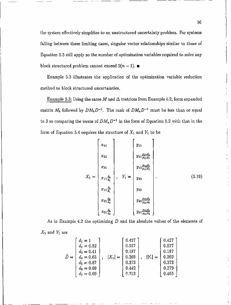
56

the system effectively simplifies to an unstructured uncertainty problem. For systems

falling between these limiting cases, singular vector relationships similar to those of

Equation 5.5 still apply so the number of optimization variables required to solve any

block structured problem cannot exceed 2(n - 1). m

Example 5.3 illustrates the application of the optimization variable reduction

method to block structured uncertainties.

Example 5.3: Using the same M and A matrices from Example 4.2, form expanded

matrix Mb followed by DMbD - 1. The rank of DMD - 1 must be less than or equal

to 3 so comparing the terms of DMaD- 1 in the form of Equation 5.2 with that in the

form of Equation 5.4 requires the structure of X, and Y to be

X11 Y1

X21 Yll pild2

pjj3dX31 Yll Ipi Id3

X- d- I 41 (5.10)

disXll dj Y51

X21d I41p 2 d4d2 P2 1 d 6

d ~P33 ds

As in Example 4.2 the optimizing D and the absolute values of the elements of

X1 and Y1 are

d-= 1 0.427 0.427d2 = 0.82 0.527 0.527d3 = 0.41 0.187 0.187

D d = 0.63, IXiI - 0.269, IY11 - 0.269d5 = 0.87 0.373 0.373d6 = 0.69 0.442 0.279d7 = 0.69 0.313 0.465

57

with p(Mb) = 6.5. Applying the MPDA property for block structures along with the

relationships of Equation 5.10 gives a simple expression for d6 (and d7) in terms of

the other di,, and the elements of P of the form

1dP21 12d 2d, J d -P3 _ 0.2267. (5.11)

Knowing that d6 is dependent on the elements of P and the other di,, allows the num-

ber of optimization variables required for this problem to be reduced from 5 to only

4. Variable reduction for other block structured uncertainties may be determined in

an analogous manner and will depend on the number and size of individual blocks.

Although Equation 5.11 is more complicated than the relationships for scalar uncer-

tainties, the elimination of unnecessary free variables should produce a net savings in

floating point operations: particularly for systems of high order.

5.4 Complete Solution to the Block 2 x 2 Problem

In the original paper introducing the structured singular value concept, Doyle

proved that for k < 3, where k denotes the number of uncertainty blocks in A, the

inequality of

IL(Mb) = sup p(MbUb) < inf '(DbMbDj') (5.12)Ub Db

is guaranteed to attain equality at the "inf" regardless of whether or not U is sim-

ple [15). For the special 2 x 2 scalar case where A has the form

A=[ ]61 b2

58

Daniel, Kouvaritakis and Latchman have shown that equality of Equation 5.12 may

still be guaranteed even though k = 4 [311. The proof for this result depends on

formulating the problem in a nonsimilarity scaling context and unfortunately does

not extend directly to handle block structured systems. However, by applying the

reduced scaling structure of the previous sections to the original proof by Doyle, it

is shown that the inequality of Equation 5.1.2 always becomes equality for any block

structured uncertainty of the form

A 1 A 2

A 3 A4

Doyle's original proof guaranteeing equality of Equation 3.22 for k < 3 requires

only that the number of independent optimization variables be less than or equal

to two [15]. Since one of the elements of scaling matrix D may always be fixed at

some arbitrary value without loss of generality, an uncertainty structure with three

or less blocks requires no more than two independent variables for the optimization

of infD (DM,,D-1 ). By proving that a 2 x 2 block structured uncertainty actually

requires no more than two optimization variables, this result may be extended to

guarantee that iz(Mb) = infDb-(DbMbD;') for general 2 x 2 block structured systems.

The following discussion briefly outlines the work of Doyle leading up to his lemma

regarding the equality of Equation 5.12 for two or less optimization variables. This

outline is presented only as a summary and the reader is referred to [15] for a complete

treatment of this material.

Before reviewing Doyle's work, a number of terms must first be defined start-

59

ing with the notion of a directional derivative for "U(D6 M6 Db1 ) with respect to the

elements of D. Denote the multiplicity of j as q and decompose (DbMbD- 1) as

(DbMbDi) ="(DbMbDR)XY 1 + Xb2bYbH

where X,, Y E Cnxq for Mb E Cn×n. Next, define some Hj such that

Hj = H1 = Re(Xff(DbMbD-1 )Y).

A directional derivative, V2 , may then be written as

V 2 = { E R',xj =vHHjvIv C',Ov -- 1}

where r represents the number of elements in the directional derivative and similarly

the number of optimization variables. Formulated in this manner, V2 simply reduces

to an ordinary gradient for q = 1. Also, for V 2 = 0 regardless of the multiplicity of

U, a true stationary point is achieved. From the MPDA theory this stationary point

assures that IL(Mb) = infDo-(DbMbDb').

The convex hull of V2, denoted coV 2, also provides gradient-type information and

for q = 1, coV 2 likewise reduces to an ordinary gradient. However, for q > 1, a value

of coV 2 = 0 indicates only that the "inf" of infDb- (DbMbD' 1 ) has been achieved

with no guarantee of a corresponding stationary point. Such a situation may actually

be a "cusp" where J(Mb) < infDb(DbMbDb').

Now let IIj = HY E Cq q, j 1,...,rand define some f : Cq R as

fj(x) = x" Hjx for x EC .

Also, for some positive integer m, let

Pm = Ix E Cm I xI = 11 C Cm

60

and

Sm = {x E Rm+ I x = 1 C Rm+1.

Using these definitions, the following lemma shows that in certain cases, V2 =coV 2.

In such cases, the condition coV 2 = 0 implies that V2 = 0 and therefore signifies that

a stationary point has been found.

Lemma 5.1: For f :Cq __ r defined as above, if r = 1 or 2, then f(pq) is convex.

Proof: See [15].

Lemma 5.1 implies that regardless of the multiplicity of V, if no more that 2

optimization variables are required to solve Equation 5.12, then V 2 =coV 2 and the

minimum of the infimization must be a stationary point and hence equals It(Mb).

The following theorem reveals that no more than 2 free optimization variables are

required to solve Equation 5.12 for systems with 2 x 2 block structured uncertainties

allowing the results of Lemma 5.1 to be invoked.

Theorem 5.3: For the case of 2 x 2 block structured uncertainties, no more than

two optimization variables are required to solve infDb'(DbMbD ') regardless of the

individual block sizes.

Proof: Define M E Cnx ' and 2 x 2 uncertainty matrix A with corresponding P

matrix as

A 1 A2 P1 Im P2 ImA=I- p

A3 A4 P I1. P4 "m

with P E -Rnx,, Pi E .mxm and m = n/2. Then similarity scaling matrix D has the

61

structure

dig di , d27.. d .., d4

Expanding the system to the form of Equations 5.2 and 5.4 and comparing terms

requires the elements of X1 and Y1 to be

XIi YIi

Xrm,1 Ym,iX(m+l),1 lI

X,= ,, = Y,,( 1 )d2 (5.13)Y(2m+l),l

Xm,1 d,1 d Y(3m),lX(rn+II d2 ),1m I "nP4 )da

2 ,1di . . (P 4 )d3

Y (drn ),l1V(P 3 )d4 J

Applying the MPDA requirement for block structured uncertainties to Equation 5.13

gives a relationship between the elements of D as

d4 = d2d3 -&(P)&(P4)di ,:P)&P3)"

Fixing d, = 1 leaves only d2 and d3 as independent variables completing the proof. n

Example 5.4: As a simple example, consider the following 4 x 4 problem with four

2 x 2 block structured uncertainties.

[ 0.8 + j0.3 1.0 + j0.9 0.1 + j0.5 0.4 + jO.5

M 1.0 + jO.4 0.7 + 10.9 0.6 + i0.5 0.8 + 3O.30.4 + yO.2 0.8 + jO.1 0.9 + j0.3 0.5 + j0.10.2 + j0.5 0.7 + jO.9 0.3 + 11.0 0.2 + 10.9

with

1 0 21 0

=A:3 A4 P=3 04 0

0 3O04

62

The singular vector relationships of Equation 5.13 become

X11 YI1

X21 Y21

X31 yu v(P2)

X41 Y]21

PddX11dj Y51

X21 dl Y61

di F (P4 )d3X3d Y516(P3 )d4

X41d aY61?(p 3 )d4

For this particular example, the optimal D is

d = 1di =1I

d2 = 1.38d2 = 1.38

D= d = 1.65d3 = 1.65d4 1.86 = dad l.

d= (2)(3)d4 =1.86 = ]-d2Tii l

=dV (2)(3)

with /(Mlb) = 16.43.

5.5 Convergence Properties of the Reduced Scaling Structure

The previous sections show that when y is found, the corresponding optimal

scaling matrix D exhibits a degree of redundancy which allows a reduction in the

numbcr of independent optimization variables. It is, however, important to ensure

that when the relationships between the dpt and pij, are incorporated in a reduced

scaling structure from the outset, the convexity properties of the original problem

63

are not lost. The remainder of this section will show that, in fact, these important

convexity properties do still apply. Furthermore, MPDA conditions used to establish

equality of Equation 3.22 for the full scaling structure also pertain to the reduced

scaling structure guaranteeing its convergence to It.

Convexity of' 2 (DMD - 1) in terms of eD, D E E) was first proven by Safonov and

Doyle [28]. Subsequent authors have offered alternative proofs in somewhat simpler

forms [35, 29]. The following lemma concerning the convexity of some function f

was proven by Tsing [361.

Lemma 5.2: Suppose Vx, gx: R 4 R twice differentiable such that f(x) = gx(x),

f(t) > g,(t) and 'g (t)j =x > 0. Then f is convex.

Proof: See [36].

Lemma 5.2 may then be applied to the scaled singular value problem to prove

convexity of -(eDi/ae-D). For notational brevity, denote M, = eDXMe - DX with

singular vectors u and v such that f(x) = "'(M) = uHMxv. Next, define g (t)

R{U"eDIAlae-DIV}. Since f(t) > g.(t) and

d- g= )It= = l H{u(D2 MAI - 2DMD + MD 2 )V}

= f(x)(u HD 2u + v"D 2v) - 2,tRu"DMDv}

= [uHD vHD] f(x)I -M. Du >0.

-Ms" f(x)I Dv

Therefore, by Lemma 5.2 f is convex.

This convexity property guarantees that any local minimum of-7(DMaD - ') with

respect to D is always a global minimum. For a new scaling matrix, S, that inherently

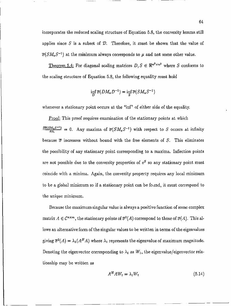
64

incorporates the reduced scaling structure of Equation 5.8, the convexity lemma still

applies since S is a subset of D. Therefore, it must be shown that the value of

-(SMkS - 1) at the minimum always corresponds to y and not some other value.

Theorem 5.4: For diagonal scaling matrices D, S E R, 2 Xn2 where S conforms to

the scaling structure of Equation 5.8, the following equality must hold

inf'(DMaD-1 ) = inf'-(SMS - 1)

D S

whenever a stationary point occurs at the "inf" of either side of the equality.

Proof: This proof requires examination of the stationary points at which

.0(SM 0S-') = 0. Any maxima of "(SMaS- 1) with respect to S occurs at infinityas,

because U increases without bound with the free elements of S. This eliminates

the possibility of any stationary point corresponding to a maxima. Inflection points

are not possible due to the convexity properties of es so any stationary point must

coincide with a minima. Again, the convexity property requires any local minimum

to be a global minimum so if a stationary point can be foand, it must correspond to

the unique minimum.

Because the maximum singular value is always a positive function of some complex

matrix A E Cnxm, the stationary points of j 2 (A) correspond to those of 5(A). This al-

lows an alternative form of the singular values to be written in terms of the eigenvalues

giving 72(A) = A1 (A"A) where A, represents the eigenvalue of maximum magnitude.

Denoting the eigenvector corresponding to A, as W1, the eigenvalue/eigenvector rela-

tionship may be written as

AHAW, =A, V1 (5.1,t)

65

and the derivative with respect to some variable x as

OAh'Aw1+ AIIAOW- = A,2 !l + WI

Sx Ox xw,.

Multiplying on the left by W-'l gives

w/H OAA WWHAHA Wl = wIHAI W + -

19 x 'O ax

which can then be simplified to

Ox" Ox W, (5.15)

giving an expression for the derivative of A, with respect to x. The derivative with

respect to some element of scaling matrix S can then be found by replacing the

variables of Equation 5.14 such that

A = AHA - S-'M D2MaS -

W1 =

A 1 =5 - .

The differentiation will first be carried out for a 2 x 2 case with respect to element

S22 of S where

S = diag[snl, S22, S33, S22S33 P11P22

P IF12P21

First decompose S such that

S = So + s 22E22 + s22s33E4,lk

where So = diag[s1 ., 0, s33, 0], k. 42P33 , and the E,, are i x i matrices with a

1 at the iith position and 0 elsewhere. Likewise, S - 1 may be decomposed as

S- 1 = So + E22 + E44822 822S33k

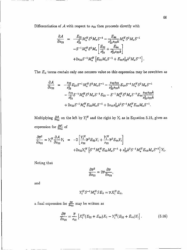
66

Differentiation of A with respect to S22 then proceeds directly with

(9A _ E22MHS2MS-1 _E4M SM,

aS 22 22 S 2 3 3-,s-Im"s mo [E22 +" E4kM322 " S- 2'S3 3 k]

+2S 2 2 S- 1 Ma [E 2 2 MaS-' + E 4 4 3 32MaS1],

The E, terms contain only one nonzero value so this expression may be rewritten as

,:-A s22E S1MHS2MS- -_ S22S33 E 4 4S - I iV4S 2 MaS-

a922 322 s 2 S3 3 k

S22S-1MHS2MaS-E 2 2 - S-IM S2MS-I E2233k

22 22S33k

+ 2S2 2S-'M E 2 2MaS-' + 2S22S -3kSM-E 4 MaS- .

Multiplying -A on the left by IH and the right by Y as in Equation 5.15, gives ana322

expression for 2 of8122

0- = Y1H O - -2 Y1H 2E 2 2 YI + LI 2E 44 y]

s 22 - 22 [22 S22 j

+2S22Y, [S-1Ma",E2 ,MS' + s4 2S- M'33°af-E 44 M. ] S

Noting that

49S22 0 22

and

Y1H S -lMIWS E =XIE i

a final expression for - may be written as

as=2 "2 [XIH(El22 + E 44 )X - Y"(E22 + E 4 4)YI] • (5.16)5S225 S22

67

Carrying out this process with respect to S33 gives an expression similar to Equation

5.16 of

= [x' (E33 + E44)X - YH(E33 + E44)Y] (5.17)833 33

Setting Equations 5.16 and 5.17 to zero establishes conditions at which the new scaling

technique reaches its global minimum. The stationary point therefore corresponds to

the value of S where

PX2 1X2 1 - Y21Y21 + T4 IX 4 - Y41Y411 = 0 (5.18)

and

[X3 1 - Y31y + T41 X41 Y41Y411 = 0 (5.19)

simultaneously.

The MPDA property guarantees that when element-by-element alignment of the

principal singular vectors of a(SMoS - ') occurs, some Ud exists such that "(SMaS -1 ) =

p(MaUd) = p(Ma). From Equations 5.18 and 5.19, such an alignment of X1 and Y

always coincides with a stationary point of 8 (SM0S=1 ) because it requires thatasi

I 211 - Y21 = IX31 - 1Y311 = IX411' - I112 = 0.

Therefore one, and hence the only, minima of-5(SMaS - 1) with respect to S must

correspond to yt(Ma) as long as some stationary point does exist.

Extension to higher order systems is simply a matter of determining which ele-

ments of S depend on a particular si. For each occurrence, an additional

Xf'EjXl - Y1H1 EjjY1

68

expression is included where the jj terms denote the elements of S dependent on a

particular si term. Again, general n x n systems similarly invoke MPDA conditions

guaranteeing that the stationary point corresponds to p(M). M

CHAPTER 6

DIRECT RELATIONSHIP BETWEEN R, L, AND D

6.1 Problem Formulation

The results of Chapter 5 show the number of optimization variables required for

similarity scaling to be no more than that required for nonsimilarity scaling. It would

therefore seem consistent that some direct relationship exists between scaling matrices

D for in1fDEV(DMaD- 1) and R and L for infR,Lw(R- 1 ML- 1 )'U(LPR) since both

methods accurately compute z. The following Theorem presents such a relationship.

Theorem 6.1: For element-by-element structured uncertainties, given some scaling

matrix D conforming to the structure of Equation 5.8, a corresponding R and L of

the form

2 _ + d+, + d.+, ".',(n-,)+, i = 2,...,n (6.1)d? + d + ... 2t~~~ ""i +d2ni n(nlU+ i

and

1 P'" n i=2,...,n (6.2)

7-1-1 --I) + I n-I)+ n(i-l)+n

may be found without further optimization such that

a(R-'ML-1 )u(LPR) = aj(DMaD-') i = 1,...,n. (6.3)

Proof: Rather than dealing explicitly with singular values, it is more convenient

in this case to use the equivalent representation

ai (A) = v,\(AHA) A E Cn×n, i 1,...n

69

71

By similarly expanding P3, B and C are found to be

2 2 ]2 22 2 12

2 2] .[P + P2 2] 2 p]2] (6.4)

C -- K. r-I1V22 + 2M1IM2- K. ['MIIM12"M22M21 + "MIM12TM21 M22]

2 2

LdI2 22

Equating &-,2 (LPR) = B and c',4 (LPR) = C, the following direct relationships

between R, L, and D will hold

but only when equality constraint

L(LPR) = [d2+ d3 P+[ 2 ] (6.5)

applies. At first glance it may appear that the constraint of Equation 6., severely

limits conditions under which Equation 6.4 holds. The remainder of the proof will

reveal, however, that this constraint simply requires the reduced similarity scaling

structure developed in Chapter 5.

The left hand side of Equation 6.5 may always be represented as A, [(LPR)" (LPR)].

Expanding matrix (LPR)11(LPR) gives

Pp2 + P2 11 2 P 2r2 + P1 2r2

(LPR)H(LPR) =P1 + 2 PIIP12 r2 + P2 iP22 l2r2

pIIp12r2 + p21p22 12r2 P2 AP2 2r 2122 P12 2 2 " 22""

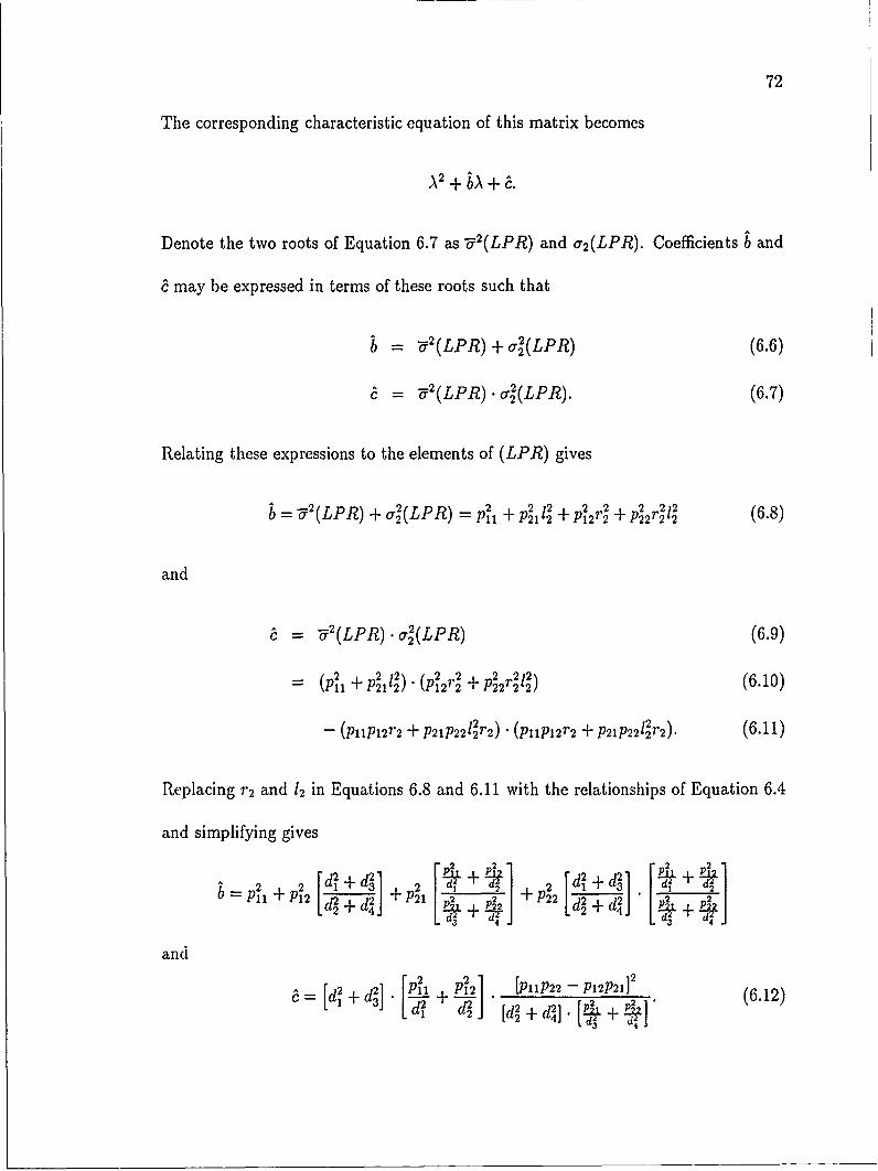
72

The corresponding characteristic equation of this matrix becomes

A2 + A + .

Denote the two roots of Equation 6.7 as "52(LPR) and a2 (LPR). Coefficients b and

6 may be expressed in terms of these roots such that

b= "2(LPR) + a2(LPR) (6.6)

= - 2 (LPR) . a2(LPR). (6.7)

Relating these expressions to the elements of (LPR) gives

21 2 2 1 2 2 2 68= (LPR) + o (LPR) =p , + p ,lt2 p 2r2 + P2r12 68

and

2 (LPR) .0,2(LPR) (6.9)

=(2 2 12) .2 2 + 2 212

11 + P21 (p12r2 P22r2/2) (6.10)

-(p, 1 Pl2r2 + p21p2212r2) " (pnp12r2 + p21P 2212 r2). (6.11)

Replacing r 2 and 12 in Equations 6.8 and 6.11 with the relationships of Equation 6.4

and simplifying gives

[d ~+d ]P2 + p2 [dl+ d32][?+ 12d2 ± 21 [+2 J 2 2 2~

and

= [d + d i] . + [1p22 -[P12P21] (6.12)

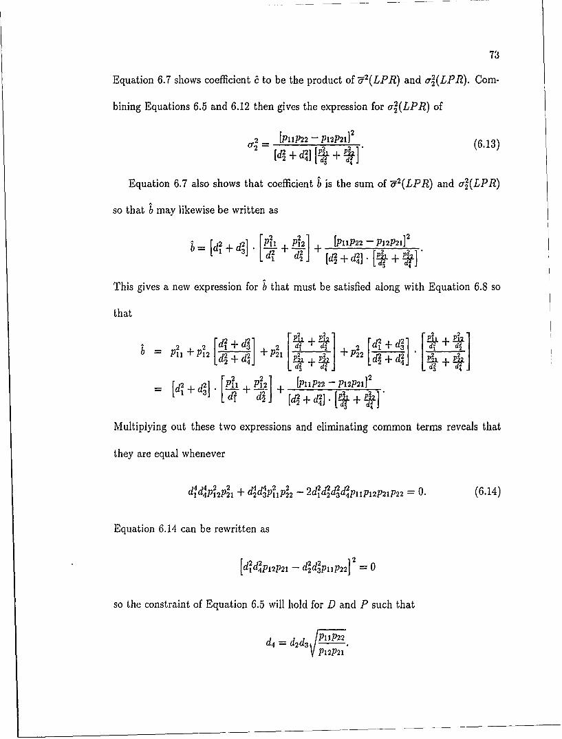
73

Equation 6.7 shows coefficient 6 to be the product of ' 2(LPR) and o'2(LPR). Com-

bining Equations 6.5 and 6.12 then gives the expression for o'(LPR) of

,2 = IPnP22 - P12P21]2 (6.13)

Equation 6.7 also shows that coefficient b is the sum of - 2(LPR) and a2(LPR)

so that b may likewise be written as

2= [[d + ][ + 4 [dP 2 ?d

This gives a new expression for b that must be satisfied along with Equation 6.8 so

that

___12 2 P L~ I [d+ d31 [221 + P222 [d2+~J "

= [d 2+d 1.[P ? p11 [P1 P22 -P12P2111 3 + - d2 A + [l~p2' +

w 2 j [d2 +d421. [1d 2

Multiplying out these two expressions and eliminating common terms reveals that

they are equal whenever

da, p12p 1 + dd pl1 p22 - 2dId d Idp1 p 12p21p22 = 0. (6.14)

Equation 6.14 can be rewritten as

[dd 2 4P12P21 - d 23PlP22 2 = 0

so the constraint of Equation 6.5 will hold for D and P such that

d4 = d2d3 P':P22fip12p21

74

This, however, is the same dependent relationship between the pi', and di,, of Equa-

tion 5.8 so the direct relationship between R and L of nonsimilarity scaling and D of

similarity scaling will always exist whenever the new scaling structure is invoked.

For the n x n case, a general expression for R and L as a function of D may

be derived in an analogous manner by comparing the characteristic equations of the

corresponding matrix systems. For M E C3X3, the characteristic equations would

contain three coefficients which must then be matched up as before. While intuitively

simple, tb- -ome too unwieldy to present here. However,

.,ation 6.4 may be written as

+ d2+1 +ddr? dn+ d2+l "" n(,,_)+l =Id + d21 + 2 ""1~~~~~ "" 22~ . dn(n-l)+i

and

I1 2 2 _=1..

PiP,.2 P:.nnd2 + T . . " " . ( = .

dn.(,-1)+1 n(s-I)+2 n(i-1)+n

completing the proof. u

The following example illustrates the application of these expressions.

Example 6.1: Using M and b from Example 4.1, optimal values for R and L are

found to be

d d2 + d2 + d 2 d 2 2 +d

r 2 = I =1.151, r3- 1d+-d 7 1.174

and- 2 22p 11+= 1 2 3 E0.9443, =

+ + 112~~ 1 3 1.203

75

with

Oi(R- 1ML-1)7(LPR) = o'i(DMaD- 1) = jt(Ma) = 8.25

u2 (R-1 ML-')a(LPR) = o2 (DMaD- ') = 5.72

o-3(R-'ML-')U(LPR) = or3(DMaD- 1) = 1.76.

It should be noted that this transformation not only provides L and A given D,

but also allows the computation of b given A and L. However, this reverse trans-

formation results in a transcendental function that must be solved iteratively. The

iterative solution is still quite fast since it involves only elementary math operations:

no singular value or eigenvalue decompositions.

6.2 Independence from M

An interesting observation concerning Equations 6.1 and 6.2 is that they are not

functions of M. This independence from M requires that any P, R, L, D combination

satisfying Equation 6.'1 for a given M, must also satisfy Equation 6.3 for any other

M. As a simple example cons:A -r the -ollowing system with two randomly generated

M matrices. [0.87 - i2.01 4.70 - i'0.0843M= M2

4.16 - iO.59 -0.92 + iO.13 2 1

1.59 1.64P 03 D = diag[1, 1.415, 1.401, 1.0571

2.81 0.83

where D satisfies the new scaling structure. Values for R ond L are found to be

R = diag[1, 0.974] L = diag[1, 0.912]

76

so that Equation 6.3 becomes

oi(TR- 1ML-)'&(LPR) = 0i(DMaD- 1) = 20.28

c92(R-'MiL--)'(LPR) = 92(DMID- 1 ) = 13.04.

Using the same R, L, and D values for A12 with no optimization gives

aj (R-IAM2L-I)-(LPR) = ,l(DM 2D -1 ) = 19.18

U2(R-IML- )-(LPR) = 9r2(DM,,2D - 1) = 1.34.

The direct relationship between R, L and D leads to the following corollary con-

cerning systems that "cusp" during the optimization process.

Corollary 6.1: Systems with element-by-element structured uncertainties with non-

simple -'(R-1ML - ') ("cusps") for nonsimilarity scaling must also produce cusps for

similarity scaling techniques and vice-versa.

Proof: The proof follows directly from the one-to-one correspondence between the

o'jq of o'(R- 1 ML-I)'u(LPR) and 'i(DAID - 1) required by Equation 6.3. a

Corollary 6.1 serves to eliminate the appealing notion that a one of these two

scaling techniques may converge to IL even if the other method fails. While some

alternative scaling technique may eventually overcome the difficulties associated with

cusping systems it is the case for nonsimilarity or similarity scaling.

Besides ruling out the use of an alternative scaling method for cusping systems,

the dircct relationship between R, L, and D serves to improve the vector optimization

method of Fan and Tits. The next chapter includes a discussion of this method and

the improvements offered by the R, L, D relationship.

CHAPTER 7REDUCTION OF OPTIMIZATION VARIABLES REQUIRED FOR THE

METHOD OF FAN AND TITS

7.1 Constrained Vector Optimization

While the scaling structure developed in Chapter 5 allows a reduction in the num-

ber of optimization variables required to compute p, the process still involves a large

number of singular value decompositions. To avoid these computationally intensive

decompositions, Fan and Tits introduced a constrained vector optimization proce-

dure that calculates p using a series of vector norms [37]. The problem formulation

is similar to the eigenvalue/eigenvector relationship for matrix A E C"nx

AW = AjW

where Wi represents an eigenvector and A, the corresponding eigenvalue. Since It(A'Ia)

is actually the solution to supu p(Ma U), there exists some supremizing U such that

IIMUIiII2 -- IIAIAj)1' 1 l)WxI2 = p(MU)IIjWII2 - p(Mo).

For IIWIl112 = 1, this reduces to IIMaOWII2 = p(MoaU) = jz(M). Defining vector

= UW1 then gives

l!MlIoAN2 = .(Ma). (7.1)

Computing the 2-norm of a complex 16 x 16 vector requires about 4n or 64 flops versus

more than 50, 000 flops for the singular value decomposition of a complex 16 x 16

77

78

matrix. Therefore, optimizing the left-hand side of Equation 7.1 offers potentially

significant numerical advantages in the calculation of y.

The optimization must first be constrained to include only "x" vectors of the form

UWi. This constraint is imposed by the Fan and Tits formulation for p(M):

i(Ma) = max {IIMoxII2 1llPiX11211MXI12 = I PiMoXIl2, i = 1,... ,m} (7.2)

where the Pi,, are projection matrices with block size m and x E C" 2. Unfortunately,

this function is nonconvex so it offers only candidate solutions. Determining whether

these candidates equal p(A'a) involves computing a corresponding scaling matrix D

from x and ensuring that IIMaJXI 2 = " (DMaD-1 ). Also, in its original formulation,

this expression requires n2 - 1 optimization variables. The following Theorem shows

that the scaling structure introduced in Chapter 5 applies to Equation 7.2 so the Fan

and Tits method actually requires no more than 2(n - 1) optimization variables.

Theorem 7.1: Given M E Cnxn and A E Cn x n , where A is composed of 1 x 1

blocks, the solution for p(MI) in the constrained optimization problem

p(Ma) = max {II IIXJi2 I IIPiXII2IIMXII2 = IIP MXII 2 , i= 1,... m)

with simple 7 can be found with no more than 2(n - J) free variables.

Proof: As in Section 5.5, denote the reduced scaling structure of Equation 5.8 as

S. Let S be the solution to infs-(SMV S - ') and Y the corresponding right singular

vector. Then the optimal solution, :, to Equation 7.2 may be written as [38]

= y

79The dependent relationships between the elements of Y may be determined using

the method of page 46. Since Y is a singular vector of SMaS- 1, any scalar multiple

of Y1 will also be a singular vector of SAIS - 1. Therefore it can be scaled such that

y1i = I without loss of generality. Likewise, .j may also be scaled to 1. Carrying out

the multiplication of S and Y1, results in a general expression of the form

I 4- fixedY2,1 - free

Yn,1

Yn+l,i *- free=)- Y Y2,lYn+l,i <-- fixed1 (7.3)

Yn,lYn+l,i - fixedY2n+l,1 - free

Y2,Y2n+l, - fixed

Y,,Y(,,-I)n+ll - fixed.Subtracting the (n - 1)2 fixed variables of Equation 7.3 from the n 2 - I free

variables previously required leaves the desired result of n2 - 1 - (n - 1)2 = 2(n - 1)

free optimization variables. u

Example 7.1 illustrates the application of Equation 7.3 to the system of Example

4.1.

so

Example 7.1: Using the system of Example 4.1, the optimal S-Y 1 may be written

as

41

Yu 211 L

2 112

8Y4

S-'Y1 Y41

Y41 --Z

83 P11 14

Y71 1S7

Y71

Scaling yii and $1 to 1 gives

1 1

Y21 1.236Y31 1.094

Y41 0.855 + 0.5191S-Y 1 = Y21Y41 = 1.056-1-0.6411

Y31 Y41 0.935 + 0.567JY71 0.355 + 0.9351

Y21Y71 0.438 + 1.1551Y31Y71 0.388 + 1.023j

with corresponding

IIMafII 2 = 8.25 = "(DMaD1 ).

7.2 Application of the Relationship Between R, L and S

As mentioned earlier, the solution to Equation 7.2 is nonconvex with many local

maxima possible. The only means of ensuring that a candidate solution vector, x,

81

actually corresponds to IL(M,) is to determine optimal scaling matrix D such that

IIMXII 2 = - (bMob -1) = (M.). (7.4)

(The method for directly computing D given x is presented in Section 8.6.) Unfortu-

nately, this singular value decomposition must be performed on the expanded n2 x n2

system for each candidate solution, reducing the overall efficiency of this technique.

However, using the direct transformation from D to R and L presented in Chapter

6, the verification test for Ip(Ma) may be reformulated as

IIMXII2 = u(R 1 VL')Y(LPR) (7.5)

where the left-hand side consists of only n x n matrices. For a system with n = 3,

the expanded n2 x n2 matrices of Equation 7.4 require about 10, 000 flops for a single

singular value decomposition. Equation 7.5, on the other hand, requires about 1,000

flops including both singular value decompositions and the required transformation

from D to L and R. Even more substantial savings occur as n increases.

The Fan and Tits method outlined in this chapter first appeared in 1985 [37].

Their constrained optimization procedure was implemented using specialized soft-

ware from the proprietary Harwell Subroutine Library [39]. Since that time, the

growing acceptance of the structured singular value concept has led to a number of

alternative formulations of t. These formulations are aimed at improving its com-

putational properties to allow for interactive design without the restrictions imposed

by the use of proprietary software. The recent announcement by the MathWorks of

the "It-Analysis and Synthesis Toolbox" for MATLAB T M indicates the demand for

82

user-friendly software to calculate A [40]. This new toolbox uses a variation of the

power method proposed by Packard, Fan, and Doyle to compute a lower bound for

p(Ma) [41]. This optimization searches for stationary points of the singular values of

(DMaD - 1) with respect to the elements of D. From the Principal Direction Align-

ment theory of Danir1, Kouvaritakis, and Latchman, such stationary points have been

shown to coincide with stationary points of p(M,,Ud) with respect to the elements of

Ud [31]. However, like all known lower bound expressions, the procedure is noncon-

vex so candidate solutions for ;(M) must be compared to the singular value upper

bound to see if they actually achieve the true supremum. Again, rather than per-

forming a singular value decomposition on the n2 x n2 system DM,D- 1, the test may

be formulated as

I5(M,,) :_ "U(R-1ML-1)75(LPR) (7.6)

involving ly n x n matrices where ii(MA) represents a candidate for p(Ma). If the

inequality of Equation 7.6 holds with equality, then Ai(Ma) ="/t(M).

If no candidate for y is found for which the lower and upper bounds become equal,

then the system may have a repeated maximum singular value at the "inf" of Equation

5.1 for scalar uncertainties or Equation 5.9 for block structured uncertainties. Lack

of stationarity at this upper bound implies that no A exists for which the upper

and lower bounds become equal. Chapter 8 contains a detailed description of the

difficulties involved with computing ji when the maximum singular value repeats.

CHAPTER 8CALCULATION OF THE STRUCTURED SINGULAR VALUE WITH

REPEATED MAXIMUM SINGULAR VALUES

8.1 Cusping Singular Values

The work presented in the previous chapters generally requires that the maximum

singular value not repeat. This requirement stems from the fact that the inequality

in the right-hand side of

It(MA,) = sup p(MaUd) < inf (DVaD- 1)Ud D

is not guaranteed to achieve equality at the "inf" if - = oi, i 5 1 because this

suggests that a stationary point with respect to D has not been found. Following the

infimization of -(DM,,D - 1) with respect to D, three possible conditions can occur.

These three conditions are illustrated in Figures 8.1 through 8.3 with corresponding

Ma matrices in Tables 8.1 through 8.3 respectively. Figure 8.1 represents a system

in which infD-5(DMaD- ') is achieved with distinct 6(DMaD-1). From the MPDA

property reviewed in Chapter 4, this guarantees the simultaneous determination of

supUd P(M,,Ud) and hence p(M,,).

Figure 8.2 represents a second system where infD'5(DM,,D-1 ) occurs with U =

'2 = supUd P(MaUd). The point at which the equalities hold will be referred to as a

"kiss" and its calculation requires special consideration.

Figure 8.3 shows a system in which infD '(DM D - 1) occurs with

= -2 # supud p(MUd) =ii(M.). This case will be referred to as a "cusp" and

83

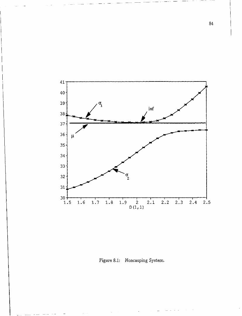
84

41-

40

39 a/ inf

38 j

37 A36

35

34

33

322

31

30 , , , ,1.5 1.6 1.7 1.8 1.9 2 2.1 2.2 2.3 2.4 2.5

D (1,1)

Figure 8.1: Noncusping System.

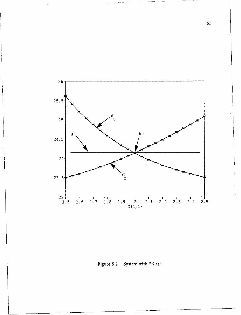
85

26

25.5

25-

24.5-

24-

23.5 2

1.5 1.6 1.7 1.8 1.9 2 2.1 2.2 2.3 2.4 2.5

D(I,i)

Figure 8.2: System with "Kiss".

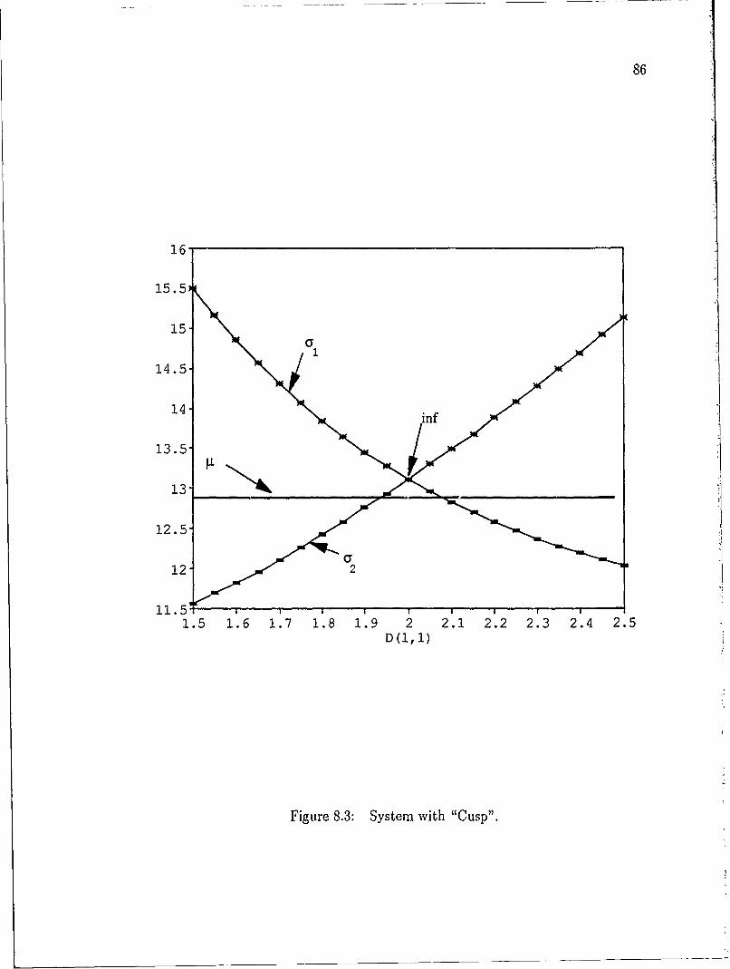
86

16

15.5)

15

14.5,

14 inf

13.5-

13 " -

12.5-

12- 2

11.5 '

1.5 1.6 1.7 1.8 1.9 2 2.1 2.2 2.3 2.4 2.5D(1, 1)

Figure 8.3: System with "Cusp".

87

Table 8.1: M Matrix for Figure 8.1.

-0.89 + 2.043 -4.34 - 5.313 -1.83 + 4.693 3.49 - 6.313 3.07 + 5.9233.87 + 17.963 1.66 - 4.721 6.83 + 2.943 -7.38 - 14.371 -8.73 - 1.293

-7.68 - 3.203 -11.10 - 8.201 6.84 - 20.10 -3.15 + 0.623 2.27 + 7.211-5.11 - 11.271 -2.81 + 14.233 8.19 + 11.803 8.89 + 14.603 2.73 - 10.693

9.83 - 18.681 -5.39 + 6.771 1.11 + 0.193 6.29 + 2.553 -2.83 + 6.753

Table 8.2: Ma Matrix for Figure 8.2.

19.18 + 0.373 6.82 - 1.753 3.13 - 0.953 -4.92 + 1.111 3.34 - 4.593-0.20 - 3.07) 18.56 + 1.293 -1.44 + 0.353 3.22 + 2.373 -1.32 + 3.153

6.42 + 1.853 -0.70 + 1.03j 15.34 - 2.013 -0.77 - 0.823 -0.13 + 1.36)0.06 + 0.641 -0.53 - 2.473 3.53 - 0.973 10.96 - 3.113 3.93 - 0.963

-2.39 - 5.34j 3.21 - 0.783 3.74 + 1.38j 3.24 - 0.033 15.41 - 0.333

Table 8.3: M, Matrix for Figure 8.3.L5.18 +0.373 6.82 -1.753 3.13 -0.953 -4.92 + 1.113 3.34 - 4591-0.20 - 3.073 4.56 + 1.29y -1.44 + 0.353 3.22 + 2.373 -1.32 + 3.153

6.42 + 1.853 -0.70 + 1.031 1.34 -2.013 -0.77 - 0.823 -0.13 + 1.3630.06+0.643 -0.53 - 2.471 3.53 -0.971 -3.03 - 3.1i3 3.93- 0.961

-2.39 -5.343 3.21 0.783 3.74 + 1.383 3.24 - 0.03j 1.41 - 0.333

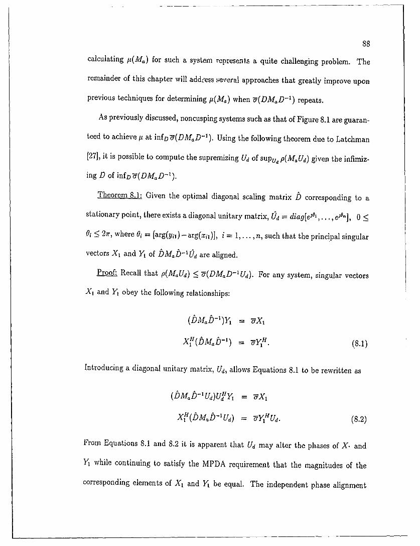
88

calculating i(Ma) for such a system represents a quite challenging problem. The

remainder of this chapter will addeess several approaches that greatly improve upon

previous techniques for determining /t(Ma) when -(DMaD- 1) repeats.

As previously discussed, noncusping systems such as that of Figure 8.1 are guaran-

teed to achieve p at infoD (DMD-1 ). Using the following theorem due to Latchman

[27], it is possible to compute the supremizing Ud of supu,, p(MaUd) given the infimiz-

ing D of infDo(DMaID-1).

Theorem 8.1: Given the optimal diagonal scaling matrix D corresponding to a

stationary point, there exists a diagonal unitary matrix, Ud = diag[elo',..., eJ'"], 0 <

Oi < 2r, where Oi = (arg(y;i)-arg(xii)], i = 1,... In, such that the principal singular

vectors X1 and Y of bMab-'Ud are aligned.

Proof: Recall that p(MaUd) < "d(DM,,D-1 Ud). For any system, singular vectors

X, and Y obey the following relationships:

(b baD-f)Y = 7X1

X1" (bAMab-') = -UyJ1 (8.1)

Introducing a diagonal unitary matrix, Ud, allows Equations 8.1 to be rewritten as

(bMab-'ud)u'Y = -ox,

x'(bMab-'Ud) = nHud. (8.2)

From Equations 8.1 and 8.2 it is apparent that Ud may alter the phases of X. and

Y1 while continuing to satisfy the MPDA requirement that the magnitudes of the

corresponding elements of X, and Y be equal. The independent phase alignment

89

of the elements of X1 and Y provides the necessary information to compute the

supremizing Ud (denoted as Ud). N

Using Theorem 8.1, the individual diagonal elements of Ud are found to be

i - eJt 9(Yi)- ar9(xi ))- e)§i' i = 1,...,n (8.3)

for element-by-element structured uncertainties. A similar expression reflecting indi-

vidual uncertainty blocks applies to the general block structured case. The actual Ud

determined in this manner is unique within some scalar multiplier eJo.

Example 8.1: Applying the relationship of Equation 8.3 with

D = diag[l, 0.460, 0.350, 0.425, 0.541], the corresponding Ud for the system of Figure

8.1 is

Ud = diag[1, 0.996 - 30.078, -0.998 + 30.060, 0.966 + 30.250, 0.921 - 30.390]

with "u(DMAD- ) = p(MaLd) = 36.94 = L(Ma).

The ability to directly compute Ld given b provides a simple means to ensure that

u(bMab- ') =iz(MA) because it guarantees that supUd p(MaUd) = infD-5(DMaD-').

This becomes increasingly important as the conditions illustrated in Figure 8.2 are

considered.

8.2 Systems with infD'5(DMaD- 1) = 02(DMaD- 1) = It(M,,)

When the singular values become equal or nearly equal, the corresponding

singular vectors become unstable with small changes in the ap, resulting in large

variations in the columns of X and Y [421. This behavior is a direct result of the

90

expressions defining the singular vectors of a matrix A, namely

AAHX, = c=aX,

AHAY = a Y. (8.4)

When the singular values repeat, the singular vectors combine to span a q-dimensional

subspace where q represents the multiplicity of the repeating oi,,. For q = 2, (the

most common case), the first line of Equation 8.4 becomes

AAHX 1 = a'X 1

AAHX2 = rX2 (8.5)

with the resulting subspace formed by the linear combination of X1 and X2 to give

AAH[(-i + 35)X + (a + )#)X 2] o[(y + jS)X 1 + (a + jf6)X 2]. (8.6)

(Note that 11 is dependent on Xi through the relationship AHX: = Coi2 and thus a

similar development for the subspaces spanned by Y and Y2 would be redundant).

From Equation 8.6 it is apparent that any linear combination of X1 and X2 satisfies

the definition of a singular vector. This arbitrariness poses a significant difficulty for

algorithms relying on the vector alignment properties of MPDA theory because there

is no longer any guarantee that vectors chosen arbitrarily from the q-dimensional

subspace will satisfy the alignment requirements.

For example, the system of Figure 8.2 has infDU(DMaD- 1) = 24.14. Using the

method of Theorem 8.1 for X 1, Y and X2 , Y2 gives corresponding values of p(MUd)

as follows:

91

XI, Y -. p(MUd) = 23.12 -1 i(Ma)

X2,1 --+ p(M,Ud) = 20.70 #y(M,)

Both the first and second principal directions must be considered in this case since

both represent legitimate solutions to Equation 8.5. The actual vectors from the

q-dimensional subspace that do provide the supremizing Ud may be found by selecting

a vector Xn, defined as

x.= ( + y5)X, + (a + 30)X 2

as in Equation 8.6. Of course Xnew is a singular vector of (Ma - ) and therefore

any scalar multiple of X,,e, is also a singular vector of (bMbD- 1). This allows the

complex multiplier (7I + 3S) of X, to be eliminated with no loss of generality leaving

only a and P3 as unknowns. Vector Xne, and the corresponding vector Y,,, may now

be written as

Xnew = XI +(a + 3)X 2

Y( b = (bMob - x (8.7)

and a 2-dimensional optimization performed over a and P3 to achieve the MPDA

conditions of aligning IXnewj and IYetlI. Assigning the complex multiplier (a + 30)

to X 2 with initial conditions of ( = / = 0 allows this procedure to be implemented

very efficiently even when - - U2. This assignment serves to initially weight X 1 more

heavily for cases with I > o'2 while still providing for subspace combinations if " and

0'2 coalesce.

92

Corollary 8.1: For systems with repeated maximum singular value of multiplicity

q with

inf*U(DM,,D -1 ) = a2(DM,,D- ) = q(DM,,D-1 ) = i(M,,),

the following condition must hold:

IL(Ma) = p(MUd) I IX,,.(ai)t - IY.o,(ai)I = 0 i = 1,...,2(q- 1). (8.8)

Proof: From the statement of the Corollary it must be possible to establish MPDA

because 5(DM, D -1 ) 0 jt(Ma) otherwise. This requires that some linear combination

of the first q columns of X and Y respectively must attain alignment. When alignment

is achieved, the equality of Equation 8.8 must hold. m

The resulting q-dimensional optimization requires only vector operations to align

X,, and Ye. Although this function is not convex, it requires only 2(q - 1) opti-

mization variables regardless of the size of the system and thus proceeds very quickly.

Example 8.2: Using the system of Figure and Table 8.2, the solution to Equation

8.8 occurs at a = -0.0009, and P3 = 0.0921. The corresponding optimal Ud is

Ud = diag[1, 0.91 + 30.43, 1.0 + 30.01, -. 94 - 30. 3 3 , 0.41 + j0.91]

with p(M,,Od) = -5(bM,,b ) = I(M,,) = 24.14.

The values of a and .8 are not robust as small changes in D cause the singular

vectors to range throughout the 2-dimensional subspace spanned by X1 and X2 . This

is important considering that algorithms used to solve infD "(DM,D -1 ) depend on the

analytic derivative, E, as developed in Section 5.5. Since the gradient is a functioa

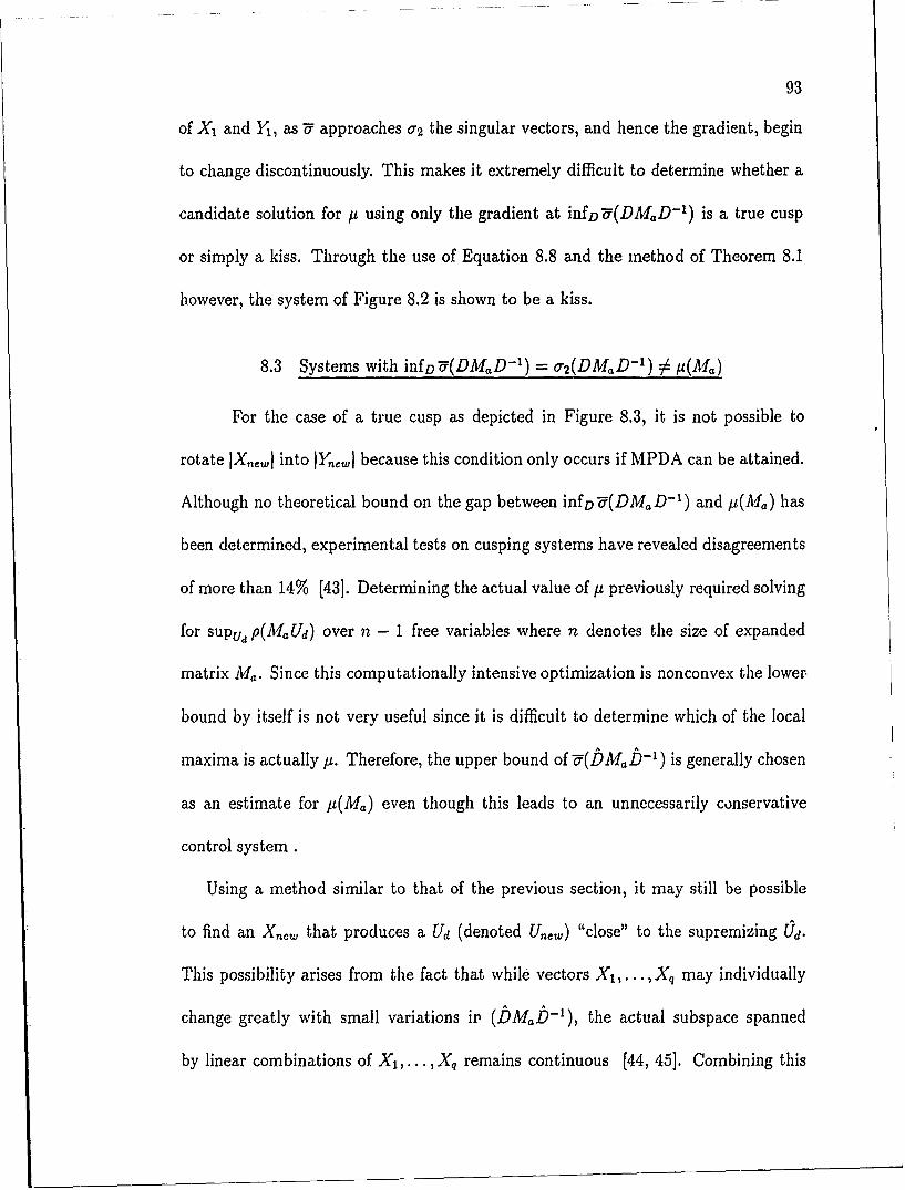
93

of X 1 and Y1, as - approaches a2 the singular vectors, and hence the gradient, begin

to change discontinuously. This makes it extremely difficult to determine whether a

candidate solution for y using only the gradient at infD-U(DMaD-1 ) is a true cusp

or simply a kiss. Through the use of Equation 8.8 and the method of Theorem 8.1

however, the system of Figure 8.2 is shown to be a kiss.

8.3 Systems with infD7(DMaD- 1) =o 2(DM,,D- 1 ) # p(Ma)

For the case of a true cusp as depicted in Figure 8.3, it is not possible to

rotate ]X,, , into IY,,,,1 because this condition only occurs if MPDA can be attained.

Although no theoretical bound on the gap between infD-d(DM,,D- 1) and y(M,) has

been determined, experimental tests on cusping systems have revealed disagreements

of more than 14% [43]. Determining the actual value of y previously required solving

for supud p(MUd) over n - 1 free variables where n denotes the size of expanded

matrix M,,. Since this computationally intensive optimization is nonconvex the lower

bound by itself is not very useful since it is difficult to determine which of the local

maxima is actually p. Therefore, the upper bound of -(bMa!b- 1) is generally chosen

as an estimate for u(M) even though this leads to an unnecessarily conservative

control system.

Using a method similar to that of the previous section, it may still be possible

to find an Xn,, that produces a Ud (denoted U,,,,) "close" to the supremizing Ud.

This possibility arises from the fact that while vectors X1,...,Xq may individually

change greatly with small variations in (bMa b-), the actual subspace spanned

by linear combinations of X1,...,Xq remains continuous [44, 45]. Combining this

94

important property with the following lemma leads to an extremely efficient method

for approximating p(Ma) for cusping systems.

Lemma 8.1: For any A E C ×nx composed of elements aij, ij = 1,..., n,

lim o (A) = lail for fixed i. (8.9)

Proof: The singular values of A are the square roots of the eigenvalues of AHA. As

an element along the diagonal of A increases or decreases towards ±oo, the remaining

elements of A become insignificant in comparison. At this point matrix product AHA

may be approximated by "t'faijE making the maximum singular value equal to

ja.i. E

Lemma 8.1 simply shows that by perturbing a diagonal element of a cusping

system, the multiplicity of U must eventually aisappear. In fact, combinations of the

diagonal elements may be perturbed providing a number of different ways to break up

a cusp. This shift eliminates the cusp and allows the establishment of MPDA for the

shifted matrix (denoted Ma) guaranteeing that infD-(DaD- 1 ) = i(Aa). MPDA

conditions also provide a direct method for computing Ud given D through the use of

Theorem 8.1. Modifying this method to use X,,,w and Y, from Equation 8.7 leads

to the following Proposition.

Proposition 8.1: Given some Ma E Cn×? for which

inf'U(DMaD- ) = o.2(DMaD- ) ... =Oq(DM,,D- ') t(M,),D

the solution over only 2(q - 1) free variables of

95

SUp p(MUo,) i = 1,... ,2(q - 1) (8.10)

is a close approximation of p(Ma).

Discussion: The continuity of the spalining subspace X, ... Xq implies that small

perturbations in the matrix elements of M will result in correspondingly small pertur-

bations in the subspace. As a scalar indication of the distance between two matrices

A, B E Cnx', define an error function E = 11A - B112 [421. Shifting the diagonal

elements of the cusping system in Table 8.3 until the cusp disappears produces a new

system with desirable MPDA properties. If this new system is sufficiently close to

the original cusping system then X,,, of the two systems should be similar.

Examination of Tables 8.2 and 8.3 reveals that the two systems are identical

except for an additive shift of +14 to all the diagonal elements of Table 8.2 so that

Ma = Ma + 14 . 5. Denote Ma and the infimizing D of Table 8.2 as M and D 2

respectively. Similarly denote the corresponding values of Table 8.3 as M,,3 and D3 .

Then

E = iD3M,3Db1 - D2Mb 2D I 16.44.

Since U(biva3 D5"1 ) = 13.11 from Figure 8.3, E indicates that the two systems are

not particularly close.

However, an alternative shift of only element Ma(1, 1) by +4 also breaks up the

cusp. Figure 8.4 and Table 8.4 show this ncw system with

[(lV) = -e(bi'IMo A 1) = 15.182.

96

18-

17.5

17-

16.5-

16- inf

15.5-1

15-

14.5-

14,

13.5-p p -

1.5 1.6 1.7 1.8 1. 9 2 2.1 2.2 2.3 2'.4 2.5D (1, 1)

Figure 8.4: System from Figure 8.3 with Shifted M,,(1, 1) Element.

Table 8.4: IvI14 Matrix for Figure 8.4.

9.18 + 0.37j, 6.82 -1.751 3.13 - 0.951 -4.92 + 1.11j 3.34 - 4591-0.20 - 3.071 4.56 +1.291 -1.44 + 0.35) 3.22 +2.371 -1.32 + 3.151

6.42+1l.853 -0.70 + 1.031 1.34 -2.011 -0.77 - 0.82) -0.13 + 1.3610.06 +0.641 -0.53 - 2.473 3.53 -0.971 -3.03 - 3.111 3.93-- 0.961

-2.39 - 5.341 3.21 - 0.78) 3.74 +1.381 3.24 -0.031 1.41 - 0331

97

Error function E then becomes

E = IDb3Ma3b3' - b 4Ma, b411[ = 4.77

indicating that System 4 is much closer to System 3 than System 2 was. Since

the spanning subspace is continuous, it seems reasonable for the optimum X,,w =

X 1 + (&I + 3&2)X 2 of the cusping system to be similar to that of Table 8.4 for which

MPDA is established. Table 8.5 shows the variation of kew as the cusping system

of Table 8.3 (Shift=0) is shifted to the noncusping system of Table 8.4 (Shift=4).

Table 8.5: Variation of kn, due to Shift of Table 8.3 System.Shift of M(1, 1)

+0 +1 +2 +3 +41 1 1 1 1

-0.053- 1 0.237 -0.070 - 3 0.248 -0.080 - j 0.254 -0.089 - 1 0.258 -0.10 - 0.260.425+ 0.210 0.424 + j 0.166 0.409 + j 0.135 0.388 + 3 0.112 0.37 + j 0.090.300+ 0.240 0.309 + 1 0.246 0.314 + 3 0.244 0.315 + 0.241 0.31 + j 0.24-0.027- j 0.345 -0.058 - j 0.352 -0.075 - j 0.355 -0.087 - y 0.354 -0.09 - 0.35

Since shifting other combinations of matrix elements will also break up the cusp,

it may certainly be possible to find noncusping systems for which E is less than the

4.77 achieved by System 4. Regardless of the shifting combination used to break up

a cusp, the 2(q - 1)-dimensional subspace spanned by X1,... , Xq must vary contin-

uously from the cusping condition to any of the noncusping conditions. This implies

that the spanning subspace is sufficiently well-behaved to provide an Xnkew from Equa-

tion 8.7 and corresponding (,,, that closely approximates UJd of P(M.(Id)- IL(a).

Although no bounds have been placed on I lie difference between sup, p(M Unew) and

supUd P(MaUd), numerical experience suggests that this di'ference is quite small. In

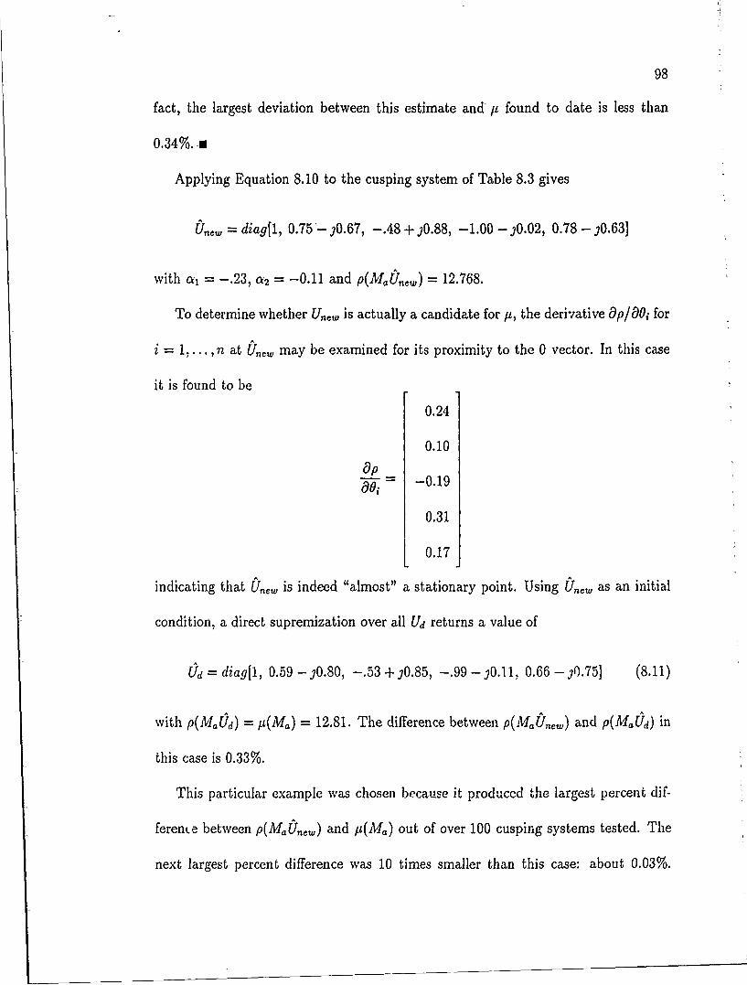
98

fact, the largest deviation between this estimate and I found to date is less than

0.34%.-a

Applying Equation 8.10 to the cusping system of Table 8.3 gives

&new = diag[l, 0.75- 10.67, -. 48 + 30.88, -1.00 - O0.02, 0.78 - 10.63]

with c = -. 23, a2 = -0.11 and p(Miew)= 12.768.

To determine whether U,,w is actually a candidate for p, the derivative 9p/O90 forA

1,... ,n at U,,ew may be examined for its proximity to the 0 vector. In this case

it is found to be

0.24

0.10

'p-O' -0.19

0.31

0.17

indicating that U, is indeed "almost" a stationary point. Using (Ue, as an initial

condition, a direct supremization over all Ud returns a value of

Ud = diag[l, 0.59 -30.80, -. 53 +30.85, -. 99 -30.11, 0.66 -30.75] (8.11)

with p(MOd) = IL(M,,) = 12.81. The difference between p(MU1r,,) and p(MOd) in

this case is 0.33%.

This particular example was chosen because it produccd the largest percent dif-

ferene between p(MaC&nw) and lz(Ma) out of over 100 cusping systems tested. The

next largest percent difference was 10 times smaller than this case: about 0.03%.

99

While larger differences are certainly possible, the fact that in the majority of ex-

amples investigated, p(Mafnew) and p(Ma(Jd) agreed within four significant figures

is most encouraging. Table 8.6 on page 114 contains a comparison between p(M)

and p(Ma U,,,) for several cusping systems. (This comparison will be discussed more

completely in Section 8.8.)

8.4 Effects of Nonconvexity

It must be emphasized that both the 2(q - 1)-dimensional search over the a

and the n - 1 dimensional search over Ud are nonconvex. Algorithms designed to

find the global maximum must employ some procedure to search the domains of Ud

or U,,, respectively. Therefore, the advantages of the 2(q - 1)-dimensional search

become more profound because the domain of Un,,,, does not increase with system

size.

Although repeated singular values with multiplicity q = n are theoretically possi-

ble, by far the more common case is for q = 2. For such systems, an additional bonus

of a 2(q - 1) = 2-dimensional search is that 3-dimensional mesh plots of p(M.Ud)

vs a, and a 2 may be generated allowing all maxima to be examined. This effectively

eliminates the difficulties of multiple maxima because all candidate points for /Z can

easily be examined.

Such a mesh plot for the system of Figure 8.3 is presented in Figure 8.5. In

this plot, a1 and a 2 range from -2 to 2. Two pronounced local maxima are readily

apparent: one corresponding to the value of p(MUne,) = 12.768 and the other at

100

61

Co

Figure 8.5: Mesh Plot of System from Table 8.3.

101

p(MaU,,ew) = 12.741 where

U.,e, = diag[1, -. 13 +30.99, 1.00 +10.084, -. 91 + jO.42, -0.81 +jO.58]

with a, = 0.25 and a2 = 0.54. Using U,, as a starting point, a search over all Ud

results in a local stationary point at

Ud = diag[l, -. 17 + jO.98, 0.95 + 30.32, -. 94 + J0.3 3 , -. 92 + 30.40]

with corresponding p(MUd) = 12.76 0 i(Ma) = 12.81.

8.5 Range of ao

The ability to ,'-.:ily select local maxima of p(M,,Un,) from a mesh plot as

candidates for p is a tremendous improvement over previous methods which require

optimizing p(MaUd) over as many as n - 1 variables, especially as the system size

increases. The range of a, an-, ' 2 used in Figure 8.4 appears to adequately cover

the subspace spanned by X1 and X 2 allowing Unew to be found. As ca1 and a 2

move away from the local maxima, the magnitude of p decreases suggesting, (but not

guaranteeing), that no additional points of interest exist outside of the plotted region.

It is important to determine the maximum range of the ai because if the bounds can

only be placed at ±o, then a mesh plot or any other search method would clearly

be impractical.

For the case of multiplicity q = 2, determining limits on a, and a 2 requires ex-

amination of Equation 8.7. Placing the complex multiplier (a1 + ya 2) on X 2 makes

the worst case condition when the optimum Xew = X2 so that X, makes no con-

tribution. Such a condition implies that at = o is required to produce the desired

102

Xn ew = X2 . However, since X1 and X2 are singular vectors they may be normalized

such that IIXI11 = [[X2 = 1. Since the 2-norm of a vector is greater than or equal to

any element of that vector, no element of X1 or X2 can be greater than 1. Therefore,

in forming X,,w = X 1 + (ail + Xa2)X 2, a1 and/or a2 values much greater than 1 will

essentially eliminate any contribution of X 1 so X,,,w quickly reaches its asymptotic

value of X2. In the rare case that such a worst case condition occurs, values of a, or

a 2 of 20 or less should be more than adequate to produce the optimum [,,,. In prac-

tice, large values of a, and/or a 2 can be eliminated by merely shifting the complex

multiplier from X2 to X 1 so that

X.W= (al + ya 2 )X1 + X 2

For Xe,,,, ; X2 , the condition of a, = a2 = 0 then prevents any contribution from

X1.

8.6 Principal Direction Alignment

The ability to compute candidates for t using only 2(q - 1) variables provides an

extremely practical means for dealing with cusping singular values. After determining

Sup', p(M.U,w) the result may compared to the singular value upper bound and if

the conservatism gap does not exceed desired tolerances no further optimization is

required. The conservative upper bound is simply chosen as an estimate for It and

the frequency sweep over the desired range continues. In the event that gap between

the upper and lower bounds exceeds the termination requirements, the supremizing

matrix O,,W offers an improved initial condition for a search over the full set (n- 1) of

103

optimization variables. Unfortunately, the computational aspects of this additional

search are potentially overwhelming: especially as the system size increases. Rather

than continuing the search for /i using eigenvalue calculations, it will be shown that a

simple transformation of U,,, allows the optimization to proceed using singular value

decompositions. Because the singular values are the square roots of the eigenvalues

of positive definite, symmetric matrices, (AHA or AAH), the singular value decompo-

sition offers significant improvements in computing efficiency over general eigenvalue

decompositions. For example, using the MATLABTM "eig" and "svd" functions on

10 random, complex 9 x 9 matrices, the average flop counts are as follows:

eig -+ 53,606 flops

svd - 38,448 flops.

As the system size increases, this difference becomes even more significant indicat-

ing the obvious computational advantage of the singular value decomposition versus

the eigenvalue decomposition. It must also be noted that the flop counts above in-

clude calculation of the singular vectors while the eigenvectors were not similarly

determined.

The MPDA property of Chapter 4 shows that the unique stationary point as-

sociated with infD -(DMaD- ') corresponds to a stationary point of supud p(MaU).

When u repeats there may be no stationary point of u so the direct relationship be-

tween u and IL is in general lost (the "kiss" condition is an exception). However, using

the principal direction alignment (PDA) property developed by Daniel, Kouvaritakis

and Latchman , a similar relationship is shown to exist between ori(DMaD- 1) and

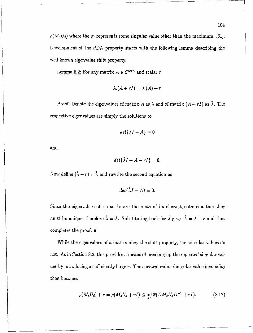
104

P(M.Ud) where the ao represents some singular value other than the maximum (31].

Development of the PDA property starts with the following lemma describing the

weil known eigenvalue shift property.

Lemma 8.2: For any matrix A E Cnxn and scalar r

Aj(A + rI) = As(A) + r

Proof: Denote the eigenvalues of matrix A as A and of matrix (A + rI) as . The

respective eigenvalues are simply the solutions to

det{AI - A} = 0

and

det{I - A - rI} = O.

Now define (5 - r) = and rewrite the second equation as

det{I - A} = 0.

Since the eigenvalues of a matrix are the roots of its characteristic equation they

must be unique; therefore A = A. Substituting back for A gives , = A + r and thus

completes the proof. a

While the eigenvalues of a matrix obey the shift property, the singular values do

not. As in Section 8.3, this provides a means of breaking up the repeated singular val-

ues by introducing a sufficiently large r. The spectral radius/singilar value inequality

then becomes

p(MaUd) + r = p(MUd + rI) _< inf'a(DMUdD-' + rI). (8.12)D

105

Equation 8.12 requires that AI(Ma Ud) corresponding to p(MaUd) be real. Such a

requirement is not a limitation, however, since Ud may be rotated by a scalar multiplier

e0 without affecting the magnitude of p(MaUd). Rewriting Equation 8.12 into a

structured singular value relationship results in

J(Ma) = sup p(MaUd) sup p(MUd + rI) - r = sup iff'j(DMaUdD- + rI) - r.Ud U Ud D

(8.13)

Unfortunately, the convexity properties that made the optimization infD -(DMaD- 1)

so attractive originally are now lost because the right-hand side of Equation 8.13 is

no longer invariant to Ud. Still, the addition of scalar r offers an alternative means

of estabhshing MPDA for cusping systems. The following theorem is originally due

to Latchman [27].

Theorem 8.2: Let "(DMaUdD - 1 + rI) have stationary points at Ud and brespec-

tively. If r is large enough to ensure that "5(bMUdD-1 + rI) is simple, then MPDA

is established for the matrix (bM]adb- ' + rI)J where J" is a matrix containing only

±1 along the diagonal and zeros elsewhere.

Proof: The stationary points of supud infDj(DMaUdD- 1 + rI) occur when

[a-(DMUdD- + rI)] = 0 (8.14)

and

(D D-+ rI)] = 0.(8.15)800.

The stationary points of Equation 8.14 have already been shown to occur upon es-

tablishment of MPDA for the matrix (DMaUdD-1 + rI). This condition applies only

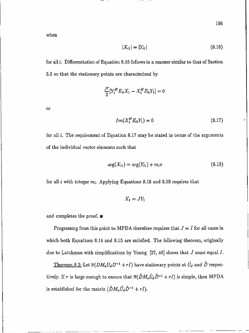
106

when

IXWI = I 1 (8.16)

for all i. Differentiation of Equation 8.15 follows in a manner similar to that of Section

5.5 so that the stationary points are characterized by

,r[yH X, - XH

or

Im(XHEiiY) = 0 (8.17)

for all i. The requirement of Equation 8.17 may be stated in terms of the arguments

of the individual vector elements such that

arg(Xni) = arg(Yj) + m"7r (8.18)

for all i with integer mi. Applying Equations 8.16 and 8.18 requires that

X1 =JY1

and completes the proof. a

Progressing from this point to MPDA therefore requires that J = I for all cases in

which both Equations 8.14 and 8.15 are satisfied. The following theorem, originally

due to Latchman with simplifications by Young [27, 46] shows that J must equal I.

Theorem 8.3: Let "(DMaUdD - 1 + rI) have stationary points at Ud and D respec-

tively. If r is large enough to ensure that "U(DMaCdb - + rI) is simple, then MPDA

is established for the matrix (bMa(Udb - ' + rI).

107

Proof: As mentioned above, this proof reduces to showing that J I at all

stationary points of Equation 8.13. Matrix (DMUdD- 1 + rI)J has been shown to

satisfy the MPDA requirement. Therefore

p(bMadb - 1 + rI) < U([bMUdb -1 + rJJ).

Multiplying by X H and X1 gives

X (bMUdD- + rI)XI _ XH(DMaUd - ' + rI)JX

which may be simplified as

rXH(I - J)X1 < X['D 'Ik UOd(J - I)X,. (8.19)

Clearly as r increases, the left-hand side of Equation 8.19 increases while the right-

hand side remains unchanged. The inequality would therefore be contradicted unless

J = I which completes the proof. n

Theorem 8.2 reveals that for r large enough to separate - and 02

sup p(MaUd) = sup inf '(DMaUdD-' + rI) - r.ud udD

More importantly, the following lemma serves to relate stationary points of

supUd infD'u(DMaUdD-1 + rI) to those of ai(DMUdD- ') where the o', represent

singular values with magnitudes less than -. This new formulation is invariant to Ud

and no longer requires the shift by r.

Lemma 8.3: For D and Ud defined as optimizing solutions to Equation 8.13, denote

X, as the left major singular vector of (DM, UdD - 1 +rI). Then X1 and its correspond-

ing conjugate transpose, XH, are also right and left eigenvectors of (bD1,aOdD - ). In

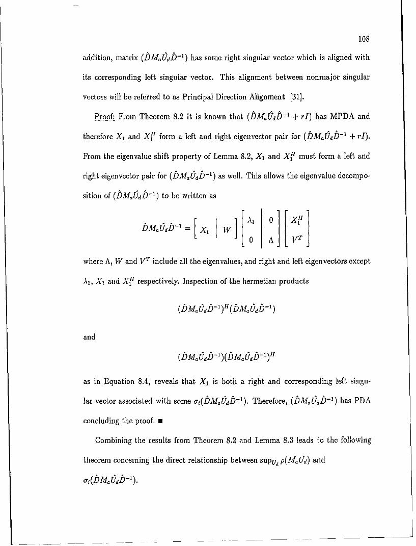
108

addition, matrix (bM,Odbl- ) has some right singular vector which is aligned with

its corresponding left singular vector. This alignment between nonmajor singular

vectors will be referred to as Principal Direction Alignment [31].

Proof: From Theorem 8.2 it is known that (bMOdb - 1 + r1) has MPDA and

therefore X, and XIt' form a left and right eigenvector pair for (DMaOdb 1 + rI).

From the eigenvalue shift property of Lemma 8.2, X1 and X H must form a left and

right eigenvector pair for (bM Odb - ) as well. This allows the eigenvalue decompo-

sition of (bMaUdD-') to be written as

bM,,adb-f = XI W A ][zz]0 A V T

where A, W and VT include all the eigenvalues, and right and left eigenvectors except

A,1, X 1 and X1f respectively. Inspection of the hermetian products

(bMaOdb- )H (bMOdb-')

and

(bMaOd1' )(b MOdb- )H

as in Equation 8.4, reveals that X1 is both a right and corresponding left singu-

lar vector associated with some oi(bMOdbD-1). Therefore, (bMOdb -1 ) has PDA

concluding the proof. m

Combining the results from Theorem 8,2 and Lemma 8.3 leads to the following

theorem concerning the direct relationship between supu, p(MUd) and

,(bMOdb-').

109

Theorem 8.4: For a-: rn.i, ri ? f, there always exists an optimal [U4 and b such

that (bMa dD-1) achie ?s ?K. and the corresponding singular value is a stationary

point with respect to D. Also, under these circumstances the following condition

arises:

sup P(Ma.Ud) =M ma oci(DMD') J [oiDMUD )= 0 (8.20)Ud '1t.7.

for ij = 1,...,n.

Proof: Theorem 8.2 guarantees the existence of an optimizing Ud and b such that

(DMaUdD- 1) satisfies MPDA. The shift property may then be employed giving

p(MAO d) = -(bM. Odb-1 + rI) - r = o(M-').

Theorem 8.3 shows that for optimal b and Ud matrix (bMaLOdb - ') will have PDA.

For the case of i = 1, - does not cusp and the MPDA property is achieved. When

i > 1, achieving PDA for (!DMadb-1) requires one of the singular vector pairs to be

aligned indicating that o'(bMa,!b - ') is a stationary point with respect to D. Selecting

the largest such stationary point completes the proof. n

Example 8.3: This example illustrates these results using the system of Table 8.3.

The supremizing Ud is the same as that presented in Equation 8.11. Infimizing the

right-hand side of Equation 8.20 over D with r > 1.87 gives

b = diag [1, 0.749, 1.106, 1.225, 1.218]

and

y (Ma) = p(M.,Od) = j(bM Odf - + rI) - r = o-2(bM.b - ) = 12.81.

110

The relationship of Equation 8.20 allows the singular value decomposition to be

retained in the computation of y even for repeated F. Unfortunately the stationarity

condition on oj no longer restricts the search for p to minima or maxima but to inflec-

tion points as well. This introduces additional complexity to an already nonconvex

function as the search criteria now includes sorting through all stationary points. If,

however, the search over the a produces a value of p(MzUet,j) close to /(Ma), then

an optimization based on the right-hand side of Equation 8.20 may offer tremendous

computational advantages over the left-hand side of the equation.

8.7 Direct Calculation of D from Ud

Section 8.6 introduced a method for directly calculating Ud given b such that

"u(bM.b-1) = P(MaUd) = /(M,). Using the 2(q - 1)-dimensional search over aj,

a candidate for Od denoted U,,e, may be calculated. In order for this estimate to

serve as a useful initial guess for the right-hand side of Equation 8.20, some means of

transforming Unetjj into a corresponding Dnew must be found. Such a transformation

was originally presented by Fan and Tits as a means of verifying that the solution

to their nonconvex vector optimization method equals 1 [38]. By modifying their

original theorem and proof pertaining to this transformation it is possible to directly

determine b corresponding to Ud such that o(DMb -1 ) = p(MOd) even when 7

repeats. Equation 7.2 is repeated here for convenience.

p((M) = max {IIMX1I2 I IIiXjI2jjMaXjI2 = IPiMXII2, i = 1,... ,m} (8.21)xE~n

111

The following proposition and subsequent theorem are originally due to Fan and

Tits with modifications to account for systems with repeated singular values [38].

Proposition 8.2: Suppose x E Cn is a solution to Equation 8.21. Then there exists

a vector )i, i = 1,... , m such that the following equation holds:

g Max + A 5 i [M',MX -PII, M"MX - IIMo a1XPiX = 0 (8.22)i=1

where the Pi are projection matrices as in Chapter 7 and the Ai,, are multipliers with

j _0, i = 1,...,n.

Theorem 8.5: Let A = [ 1,...,An] be the unique multiplier vector corresponding

to the optimizing . Then/ =a diag [),... , A ] is the solution to Equation 8.20.

Proof: From Chapter 7, some Y1 must exist such that

b-'/2M Y, = b(o- 1) y, = y,2(Ma)y, IIMaXI2Y,.

Multiplying on the left by b gives the expression

M b 2MaX IIMaXJ 2b2. (8.23)

Now define some P6 such that

Pi = ad i= 1,...,m (8.24)

with a selected such that EL1 IldI1xl 2 - 1. Then a=P2 E}z3(Pi and Equation

8.23 becomes

Epi [iVPMalMX - IMaXJI1'pX] 0i-1

givingn

MH MaX + Z8, [MapiMaX - IPXIIMH MaX - IIMaxliJpX] = 0.i=1

112

Equating fl = Ai, this equation becomes identical to Equation 8.22 and through the

relationship of Equation 8.24 the proof is complete. n

It is now possible to directly determine a/D given (d such that

p(M. Ud) = oi(bM D-1) = i(M)'. Again using Od from Equation 8.11,/ Dis found

to be

= diag [1, 0.749, 1.106, 1.225, 1.218]

with

ti(M) = p(M.Od) = '2(!bM,!b-') = 12.81

providing the same results as before. However, no additional optimization is required

for this method as opposed to Example 8.3 which requires an infimization over D of

-5(DMaUdD- 1 + rI). Provided that the 2(q - 1)-dimensional optimization generates

a U,, close to Ld, the transformation from U,,, to Dn,,, may be invoked to solve

for it using the method of Equation 8.20.

8.8 Comparison of Optimization Methods

The results of this chapter are summarized in Tables 8.6 and 8.7. Table 8.6

lists system size, the results of infD'(DM'ID-1), the value I(Ma ), the results of

sup,, p(MAU ew), and the per cent difference between it(Ma ) and sup,, p(MUe,,).

System 6 corresponds to that of Figure 8.3 and, as mentioned earlier, it shows the

largest deviation between 1 (M) and sup,,, p(MU.c,) of all cusping systems studied

to date. System 5 shows the largest deviation between infD'(DMD - ') and u(jMv/')

while the corresponding value of sup, p(MU,,,,w) equals I(Ma ) within four significant

113

figures. Clearly the result of the 2(q - 1)-dimensional optimization sup, p(MaUew)

provides an excellent estimate of y.

Depending on the particular control system under development, it is likely that

these estimates of y will be satisfactory without any additional optimization. In the

event that i must be determined exactly, the optimum U,, from sup, p(MU, ,)

may be used as an starting point for further searches. Using the same systems as

Table 8.6, Table 8.7 summarizes the flop count requirements of the various methods.

Each of the optimization methods call a series of MATLABTA m-files developed

by Grace [33). While m-files generally execute more slowly than compiled code, the

ability to track flop counts provides a means of comparing the efficiency of algorithms

regardless of the host machine.

In order to provide as equitable a comparison between methods as possible each

cusping system was required to satisfy three criteria. Of all cusping syfjtems tested,

only those meeting these criteria are included in Tables 8.6 and 8.7. (Note: It should

be mentioned that failure to satisfy these criteria does not mean that the optimization

methods could not find t for a particular system, it simply means that any flop count

comparison would be erroneous.)

The first selection criterion is that optimization methods A and B (supud p(MUd)

and supa, p(MaU,l.,) respectively), must begin at the same starting point. This point

is a value of Ud generated by the method of Theorem 8.1. For q = 2, two values of

Ud are generated with U1 corresponding to X, and Y1 and U2 corresponding to X2

and Y2 . Since these singular vector pairs are effectively interchangeable at the cusp

114

Table 8.6: Cusping Systems% Difference

System Size infva(DMaD-1 ) pL sup,. p(MaUn,,) p2 vs p(MU,,)1 4 6.8125 6.7803 6.7803 -0.0002 4 5.9398 5.9015 5.9015 -0.0003 4 7.1238 6.9697 6.9488 -0.0134 4 6.5750 6.3673 6.3671 -0.0035 4 1.0322 0.9470 0.9470 -0.0006 5 13.114 12.810 12.761 -0.3267 5 31.710 31.443 31.440 -0.0098 5 35.838 35.615 35.604 -0.0319 5 43.913 43.809 43.807 -0.00710 5 35.126 34.930 34.922 -0.02211 9 7.7400 7.7394 7.7394 -0.00012 9 7.8366 7.8346 7.8346 -0.00013 9 9.7072 9.6193 9.6185 -0.00814 9 29.473 29.254 29.253 -0.00315 9 128.02 127.07 127.07 -0.00216 9 74.749 74.502 74.501 -0.00117 9 151.95 150.29 150.28 -0.00218 9 209.64 209.21 209.20 -0.00119 9 35.238 34.610 34.610 -0.00120 9 35.918 35.339 35.336 -0.008

115

Table 8.7: Floating Point Operations ComparisonOptimization Method

A B C DBI BI

System supu,p(MUd) sup,, p(M,,Uew) supu p(M,,Ud) maxi oi(DM.D - )1 234,427 128,578 149,067 149,8992 138,177 113,174 144,883 150,3543 128,398 136,015 191,239 157,3724 188,109 193,382 212,596 214,3735 171,721 63,162 74,317 79,787

Average: 172,166 126,862 154,420 150,3576 579,929 301,294 395,592 343,1737 382,910 299,005 550,583 343,3138 709,431 285,912 452,255 329,6349 839,772 553,011 722,400 595,73310 415,088 256,610 582,077 300,868

Average: 585,426 339,166 540,581 382,5,411 677,513 226,805 408,046 452,39012 1,037,283 384,400 563,199 611,34613 1,992,286 816,698 1,221,836 1,039,923.4 2,909,386 1,172,394 1,850,040 1,398,54215 2,850,485 1,078,454 2,345,768 1,307,23816 3,203,488 984,491 1,952,090 1,211,70117 3,327,218 1,240,607 2,200,240 1,465,97718 2,786,795 1,330,380 2,342,328 1,556,34619 3,349,508 946,319 1,687,675 1,113,34520 4,492,976 1,684,968 3,521,077 1,937,664

Average: 2,662,694 986,551 1,809,229 1,109,472

116

(see Equations 8.4 and 8.5), both U1 and U2 provide candidate starting points for

the subsequent optimizations. The choice between the two is made by selecting the

maximizer of p(MaUi) for i = 1,... , q. The extra flops required to select the desired

Us are generally more than offset by increased convergence rates resulting from the

superior starting point.

Choosing U, or U2 as a starting point for supud p(MUd) corresponds to choosing

whether the complex multiplier (a' + ja2) acts on X, or X 2 in Equation 8.7. Using

al = a 2 = 0 as an initial condition, matrix U1 results from

X.e = X1 + (al + Ja 2)X2

while U2 results from

X.ew = (a, + a 2)XI + X 2 .

This procedure allows supud p(MaUd) and sup, p(MaU,,,) to start at the same point

satisfying the first selection criterion.

The second criterion requires the optimization to converge to y from the common

starting point. This greatly reduces the number of systems available for flop count

comparisons because the methods are all known to be nonconvex. While changing

the initial starting points would eventually lead to /j, the possibility of an equitable

flop count comparison is eliminated. This local convexity criterion extends to the

methods of columns C and D of Table 8.7 as well. For these methods, sup,, p(AIaUew)

provides an improved starting point for subsequent optimizations by supud p(MaUd)

and maxjor(DM D - 1) respectively. As discussed in Section 8.6, the optimization

based on ai(DM,,D- 1) searches for all stationary points including maxima, minima,

117

and inflection points. While the computational advantages of the singular value

decomposition makes it quite fast, its nonconvexity generally prevents its use without

the improved starting point provided by sup, p(MUew).

The final selection criterion involves termination conditions for the separate meth-

ods. While the end results of methods A, C, and D should be identical, differences in

problem formulation prevent the use of a common termination condition. If one algo-

rithm employs a more strict termination condition, it may unnecessarily require more

flops than a second, less strict method to achieve the same results. To resolve this

dilemma, parameters were adjusted to halt the optimization of supu, p(MaUd) when

11 a"11< 0.02. Corresponding parameters for maxi o'(DMaD- 1) were then set such

that termination occurred when maxi oi(DM D - 1) = p(MOd) within four significant

figures.

Termination conditions for sup,, p(MaUn,,,) were adjusted such that the optimiza-

tion successfully halts when all terms of the numerical gradient fall below 102. Tests

with varying termination conditions suggest that further reductions in the numerical

gradient produce little if any improvement in p(MaUnew).

Having discussed the three selection criteria, the flop count comparison of Table

8.7 may be examined. The superiority of Method B in terms of computing efficiency

is immediately apparent. For the 4 x 4 systems, an average of 172,166 flops was

required by Method A versus 126,862 flops for Method B: a savings of 26%. This

savings increases to 42% for the 5 x 5 systems and 63% for the 9 x 9 systems. For

118

design problems requiring exact values of p, Method D offers a savings of 58% over

Method A and 39% over Method C for 9 x 9 systems.

The efficiency of Method D for finding the exact value of u seems to be a direct

result of the excellent starting point provided by first solving for sup, p(MUJew).

In fact, for many of the 20 systems the flop count difference between Methods B

and D simply refl,!cts the calculations involved in computing -'M one time. The

resulting derivative was sufficiently small to meet the termination criteria without

further optimization.

It is important to emphasize that the criteria chosen for the flop count com-

parison, especially the second criterion, actually skew the results against the new

2(q - 1)-dimensional search method. While the flop count savings are quite substan-

tial, the real advantages occur for systems that do not directly converge to i from

the starting point. Convergence to some local maxima requires the selection of a new

starting point from which the search for jt may continue. For previous methods thi

means a search over n - 1 dimensions so the search area grows exponentially as sys-

tem size increases. The new method, however, requires a search over only a 2(q - 1)

dimensional space greatly increasing the likelihood of quickly finding /L.

8.9 Algorithm for Cusping Systems

Certainly the numerical efficiency of sup, p(MUnt,) offers advantages even if

the exact value of y must be found. For the general cusping case of q = 2, the ability

to generate and view 3-D mesh plots as in Figure 8.4 offers a means of partially

overcoming the problem of nonconvexity. A general algorithm for computing I to

119

account for cusping and noncusping systems is now presented.

1. Compute infD (DMD-1 ). If MPDA is established then 7(bMb - ) = 1t(MA)

and the algorithm is complete.

2. If MPDA is not established then no stationary point was found and the sys-

tem is either a "kiss" or a "cusp." Determine the first q singular vectors of

(DM,,D- l) where q is the multiplicity of U and compute sup,, p(M.U, o). If

MPDA is now established ("kiss") or p(M,,U,,t,) is within some allowable dis-

tance of "(DiaD- l) at the cusp then the procedure is complete and upper

bound "(DM,,D -1 ) is used for A(M).

3. If p(Malntu) falls below the desirable distance from "F(DMaD- 1) then continue

with the PDA search over oi(DM,,D- ') (Method D of Table 8.7) to determine

a true stationary point.

4. If the stationary point from Step 3 is still not acceptable then either change

the initial settings of the ai and repeat Steps 2 and 3 or generate a mesh of

p(MUn,,,) over the cei as discussed in Section 8.4. Then investigate all local

maxima from the mesh for the global maximum of supun p(MaUd).

While even the mesh is not guaranteed to contain y, the advantages offered by the

optimization sup,, p(MaU,,,w) are a tremendous improvement over previous methods

of computing jt for cusping systems. It should also be mentioned that this approach

for computing p also extends to cusping block structured systems. Equation 5.10

reveals the relationships between the elements of X 1,... ,Xq and Y1,..., Yq which

120

musl, hold even when cusping occurs. Similar relationships can be determined for any

general block structured system so forming X,, as linear combinations of X1,..., Xq

proceeds exactly as before. The only difference between the element-by-element un-

certainty algorithm and that for general block structured systems is in the formulation

of U,,,, which must reflect the associated block configuration. Otherwise, the same

reduction in optimization variables with corresponding efficiency benefits applies.

CHAPTER 9CONCLUSION

9.1 Summary

This dissertation presents new results in the area of stability robustness analy-

sis for multivariable systems. Of primary significance are the links developed between

similarity and nonsimilarity scaling techniques for computing the structured singular

value (y). The results of Chapter 5 show that no more than 2(n - 1) optimization

variables are required to compute y using either similarity or nonsimilarity scaling.

While the nonsimilarity scaling approach effectively addresses element-by-element

structured uncertainties, the ability of similarity scaling to handle general block struc-

tured uncertainties with no more than 2(n - 1) free variables greatly simplifies the

calculation of i for this important uncertainty class.

For the general block 2 x 2 problem, the elimination of redundant variables leads

to a guarantee that the solution of infD, 7(DbMbDg') equals (Mlb) regardless of

whether or not a stationary point occurs at the "inf." This eliminates the need to

employ one of the computationally intensive lower bound optimization routines for

this class in the event that the maximum singular value repeats.

In addition to the reduction in optimization variables, the link between the two

scaling methods is shown in Chapter 6 to include a direct relationship between scaling

matrix D of similarity scaling and scaling matrices R and L of nonsimilarity scaling.

121

122

The value of this direct relationship is shown to be most evident when applied to

methods that compute a lower bound for y as described in Chapter 7. Since such

methods involve nonconvex optimizations, their solutions are initially ,cnly candidates

for y. Guaranteeing that some solution actually equals p requires showing that the

candidate and the upper bound of!(bMa,,b1) are equal. Computing the correspond-

ing b for a particular j candidate is straightforward; however, the actual singular

value decomposition must then be performed on D and Ma matrices with dimensions

as large as n2 x n2. By directly transforming b to the corresponding A? and L, the

upper bound may be determined using the n x n decomposition U(T- 1ML - )U) ( _P / )

with a substantial reduction in floating point operations for each step in the required

frequency sweep.

One of the most important advantages of computing the singular value upper

bound for y is that any local minimum must be the global minimum. As long as

this minimum corresponds to a stationary point, the MPDA theory guarantees that

this upper bound equals 1. However, for those cases that do not achieve stationarity

at the minimum ("cusps"), I is not achieved and, in fact, the actual value of pZ may

differ from the upper bound by more than 15%. Because of the nonconvexity involved

in lower bound calculations and the dangers of choosing an optimistic estimate for

pi, the conservative upper bound is generally used in place of p when cusping occurs.

This is particularly true as system size increases because the lower bound solution

domain increases directly with n, greatly impeding the search process.

By applying the MPDA principal, an estimate for I requiring only 2(q - 1) op-

123

timization variables (where q denotes the multiplicity of the cusp) is proposed in

Chapter 8. The largest deviation found to date between this estimate and the actual

value of 1 is less than 0.34%: well within most real-world engineering tolerances.

Reductions in floating point operations of more than 60% for 9 x 9 systems are ex-

perienced versus previous methods and for the most common cusping case of q = 2,

3-dimensional mesh plots may be used to easily locate candidates for p. The a

estimate holds for cusping systems with element-by-element as well as block struc-

tured uncertainties so any system with structured uncertainties can benefit from this

method. Also, the estimate can serve as an initial st rting point in the event that

Ip must be determined exactly. Such a procedure employing the Principal Direction

Alignment theorem is shown in Table 8.6 to find the actual value of P with only a

slight increase in floating point operations over that required for the estimate.

9.2 Future Directions

9.2.1 Nonsimilarity Scaling with Block Structured Uncertainties

The results of this dissertation serve to enhance many of the important tools

used to analyze the robust stability properties of multivariable control systems. In

the process of completing one particular objective, other promising areas frequently

appear as directions for additional research. One of the more intriguing of such

areas emerging from this work is the possibility of adapting the nonsimilarity scaling

technique to work with general block structured uncertainties.

For element- by-element structured uncertainties, the advantages of nonsimilarity

scaling are quite clear. For example, using the similarity scaling approach, System

12 of Table 5.2 required 922,383 flops to compute p using the reduced scaling struc-

ture. For the same system, the nonsimilarity scaling approach required only 105,061

flops: a reduction of more than 88%. Unfortunately, current nonsimilarity scaling

formulations do not treat general block structured uncertainties so the tremendous

advantages cannot be realized for this important uncertainty class.

While uncertainty blocks with arbitrary dimension currently prevent the use of

nonsimilarity scaling methods, the direct relationship between D, R, and L of Chapter

6 may be applied to at least one specific block structure. This structure rcquires

only that all the blocks be of a common size so that more than the standard scalar

uncertainty elements are allowed. To illustrate the application of nonsimilarity scaling

to this class of uncertainties, consider the system of Example 5.4 on page 61. A direct

calculation of /?, and L from b gives

"R= diag[l, 1, 0.833, 0.833], L diag[1, 1, 0.625, 0.6251

with -(Rh-ML-'d(LPR) = -(bMb" ) 16.43 = 1(Mb). Since the direct trans-

formation holds here, the problem could have been solved by employing nonsimilarity

scaling from the start. The ability of nonsimilarity scaling to address even this limited

class of block structured uncertainties combined with the correspondence between op-

timization variable requirements suggests that some general block uncertainty form

of nonsimilarity scaling may eventually be possible.

9.2.2 H-' and i-Synthesis Design Methods

Two recent advances in the design of multivariable control systems are the

HiI and ji-synthesis methods. The HOO technique allows for the design of controllers

125

that possess optimal performance in terms of minimizing the HI norm of some fre-

quency dependent transfer matrix [18]. On the other hand, j-synthesis extends

the optimal performance properties of the H- method to encompass robust perfor-

mance characteristics as well [19]. A number of interesting design studies involving

the p-synthesis approach have appeared including a flexible antenna structure and

an implementation of the space shuttle lateral axis flight control system [47, 481. The

next few paragraphs give a brief overview of these techniques along with possible

applications of the retdts of this dissertation.

For transfer matrix G, the HOO norm of G may be written as

IIG(s)Ik = sup-(G(s)) (9.1)

where s again denotes frequency dependence [49]. Figure 9.1 depicts the standard

H00 system model with feedback controller K. Transfer matrix G can be partitioned

as

G = (9.2)G21 G22

giving a set of system equations of the form

z = Glw + G12u, y = G21w + G22u.

Noting that u = Ky allows this to be rewritten as

z = [Gil + G12K(I - G22K)'G 2i]w (9.3)

Defining F = [C1 + G12K(I - G22K)-G 2 ] as the transfer matrix from external

input, w, to output z, Equation 9.3 can then be written as

Z = Fw.

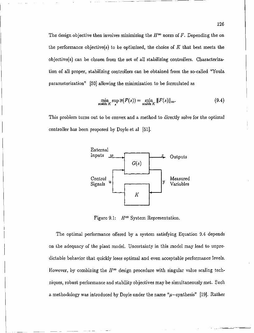
126

The design objective then involves minimizing the H- norm of F. Depending the on

the performance objective(s) to be optimized, the choice of K that best meets the

objective(s) can be chosen from the set of all stabilizing controllers. Characteriza-

tion of all proper, stabilizing controllers can be obtained from the so-called "Youla

parameterization" [50] allowing the minimization to be formulated as

min supu(F(s)) = min IIF(s)JI.. (9.4)

stable Ks stable K

This problem turns out to be convex and a method to directly solve for the optimal

controller has been proposed by Doyle et al [511.

ExternalInputs w - 4 Outputs

Control MeasuredSignals u Y Variables

K

Figure 9.1: HOO System Representation.

The optimal performance offered by a system satisfying Equation 9.4 depends

on the adequacy of the plant model. Uncertainty in this model may lead to unpre-

dictable behavior that quickly loses optimal and even acceptable performance levels.

However, by combining the HII design procedure with singular value scaling tech-

niques, robust performance and stability objectives may be simultaneously met. Such

a methodology was introduced by Doyle under the name "y -synthesis" [19]. Rather

127

than simply minimizing "U(F(s)) as a function of frequency and stabilizing controller,

K, pt-synthesis allows for the incorporation of structured plant uncertainties with

the design objective of solving

min if IIDPD-1 1100 (9.5)stable K D

where represents the appropriate combination of F and A. For fixed D, Equation

9.5 is a standard H'0 problem. Similarly for fixed K the problem involves finding

,t(DFD- 1). Separately, each problem is convex. Unfortunately, the combined prob-

lem loses this desirable convexity property so there is no guarantee of ever achieving

the global minimum in terms of both K and D.

While the I-synthesis approach provides controllers with robust performance, it

requires a tremendous amount of computing power to find even a local minimum of

Equation 9.5. With the loss of convexity, computational requirements increase even

more. However, by applying the results of this dissertation, it may be possible to

improve the efficiency of the p-synthesis method.

For example, the reduction of optimization variables for systems with both scalar

and block structured uncertainties should directly apply to that step of the procedure

involved in infimizing the maximum singular value over D. Also, the direct relation-

ship between similarity scaling matrix, D, and nonsimilarity scaling matrices L and R

might provide insight into a formulation of p-synthesis involving only nonsimilarity

scaling with its corresponding reduced system size. Finally, the procedure outlined

in Chapter 8 for estimating p with a repeated maximum singular value should apply

to the p-synthesis problem when cusping occurs so that unnecessary conservatism

128can be reduced without the huge computing cost involved with previous methods of

determining the lower bound for y.

Although the actual benefits of applying the results of this dissertation to the/t-synthesis design approach are as yet unknown, any efficiency advantage over pre-

vious methods is certainly welcome. Since all but the simplest of design problems

require tradeoffs between performance requirements, an iterative process is normally

employed to achieve a satisfactory performance compromise. Efficiency improvements

as low as ten or twenty percent could therefore translate into several hours worth of

CPU savings as an acceptable performance trade-off is reached.

REFERENCES

1. L. Ljung, System Identification, Prentice-Hall, Englewood Cliffs, NJ, 1987.

2. B. Friedland, Control System Design, McGraw-Hill, New York, 1986.

3 A. Yue and I. Postlethwaite, "Improvement of Helicopter Handling QualitiesUsing H'O-Optimisation," Proc. TEE, vol. 137, Pt. D, no. 3, May 1990, pp.115-130.

4. F. Nesline and S. Joshi, "Aerospace Control Systems," IEEE Control SystemsMagazine, vol. 10, no. 4, June 1990, pp. 3-4.

5. M. Morari, and E. Zafiriou, Robust Process Control, Prentice Hall, EnglewoodCliffs, NJ, 1989.

6. H. 5. Black, "Stabilized Feed-Back Amplifiers," Electrical Engineering, vol. 53,Jan. 1934, pp. 114-120.

7. H. S. Black, "Inventing the Negative Feedback Amplifier," IEEE Spectrum,Dec. 1977, pp. 55.60.

8. H. Nyquist, "Regeneration Theory," Bell Systems Tech. J., vol. 11, 1932, pp.126-147.

9. H. Bode, Network Analysis and Feedback Amplifier Design, Van Nostrand, NewYork, 1945.

10. P. Dorato, "Robust Control: A Historical Review," Proc. IEEE 2 5th CDC.,1986, pp. 346-349.

11. A. MacFarlane, and I. Postlethwaite, "The Generalised Nyquist Stability Crite-rion and Multivariable Root-Loci", Int. J. Control, vol. 25, 1977, pp. 81-127.

12. J. Doyle and G. Stein, "Multivariable Feedback Design: Concept for a Classi-cal/Modern Synthesis," IEEE Trans AC, vol. AC-26, 1981, pp. 4-16.

13. "Challenges to Control: A Collective View," IEEE Trans AC, vol. AC-32, 1987,pp. 275-285.

14. M. Safonov, "Stability Margins of Diagonally Perturbed Multivariable FeedbackSystems," TEE Proc., vol. 129, Pt. D, no. 6, Nov. 1982, pp. 251- 256.

129

130

15. J. Doyle, "Analysis of Feedback Systems with Structured Uncertainties,"Proc. IEE, vol. 129, Pt. D, no. 6, Nov. 1982, pp. 242-250.

16. B. Kouvaritakis and H. Latchman, "Singular Value and Eigenvalue Techniquesin the Analysis of Systems with Structured Perturbations," Int. J. Control, vol.41, no. 6, 1985, pp. 1381-1412.

17. B. Kouvaritakis and H. Latchman, "Necessary and Sufficient Stability Crite-rion for Systems with Structured Uncertainties: The Major Principal DirectionAlignment Principle," Int. J. Control, vol. 42, no. 3, 1985, pp. 575-598.

18. G. Zames, "Feedback and Optimal Sensitivity: Model Reference Transforma-tions, Multiplicative Seminorms, and Approximate Inverses," IEEE Trans AC,vol. AC-26, 1981, pp. 301-320.

19. J. Doyle, "Structured Uncertainty in Control System Design," Proc. 2 4th CDC.,Ft Lauderdale, FL, Dec. 1985, pp. 260-265.

20. Y. Foo, "Robustness of Multivariable Feedback Systems: Analysis and OptimalDesign," D. Phil. Thesis, Oxford University, Oxford, England, 1985.

21. J. M. Maciejowski, Multivariable Feedback Design, Addison-Wesley PublishingCompany, Wokingham England, 1989.

22. R. Smith and J. Doyle, "Model Invalidation: A Connection between RobustControl and Identification," Proc. ACC, 1989, pp. 1435-1440.

23. M. Fan, A. Tits and J. Doyle, "Robustness in the Presence of Joint ParametricUncertainty and Unmodeled Dynamics," Proc. ACC, 1988, pp. 1195-1200.

24. R. De Gaston and M. Safonov, "Exact Calculation of the Multiloop StabilityMargin," IEEE Trans AC, vol. AC-33, no. 2, Feb. 1988, pp. 156-171.

25. R. Pefia and A. Sideiis, "Robustness with Real Parametric and StructuredComplex Uncertainty," Proc. IEEE 271h CDC., 1988, pp. 532-537.

26. P. Young and J. Doyle, "Computation of the Structured Singular Value withReal and Complex Uncertainties," Proc. IEEE 2 9th CDC., 1990.

27. H. Latchman, "Frequency Response Methods for Uncertain Multivariable Sys-tems", D. Phil. Thesis, Oxford University, 1986.

28. M Safonov and J Doyle, "Optimal Scaling for Multivariable Stability MarginSingular Value Computation," MECO/EES '83 Symposium, Athens, Greece,Aug. 29-Sep. 2, 1983, pp. 466-469.

29. R. Sezginer and M. Overton, "The Largest Singular Value of eXAoe- x is Convexon Convex Sets of Commuting Matrices," IEEE Trans AC, vol. AC-vol. 35,no. 2, Feb. 1990, pp. 229-230.

131

30. E. Osborne, "On Pre-Conditioning of Matrices," J. Assoc. Comput. Mach.,1960, vol. 7, pp. 338-345.

31. R. Daniel, B. Kouvaritakis, and H. Latchman, "Principal Direction Align-ment: A Geometric Framework for the Complete Solution to the ti-Problem,"IEE Proc., vol. 133, Pt. D, no. 2, Mar. 1986, pp. 45-56.

32. PC-MATLAB User's Guide, The MathWorks Inc., South Natick, MA, 1989.

33. A. Grace, "Computer-Aided Control System Design Using Optimization Tech-niques," Ph.D. Thesis, University of Wales, Bangor, England, 1989.

34. W. Press, Numerical Recipes: The Art of Scientific Computing, Cambridge Uni-versity Press, New York, NY, 1986.

35. J. Doyle and C. Chu, "Robustness Control of Multivariable and Large Scale Sys-tems," Final Technical Report for AFOSR, Contract F49620-84-C-0088, Mar.1986.

36. N. Tsing, "Convexity of the Largest Singular Value of eDtle-D: A ConvexityLemma," IEEE Trans AC, vol. AC-35, no. 6, June 1990, pp. 748-749.

37. M. K. H. Fan and A. L. Tits, "A New Formula for the Structured SingularValue," Proc. IEEE 2 4th CDC., 1985, pp. 595-596.

38. M. K. H. Fan and A. L. Tits, "Characterization and Efficient Computationof the Structured Singular Value," IEEE Trans AC, vol. AC- 31, no. 8, pp.734-743, Aug. 1986.

39. "Harwell Subroutine Library," Library Reference Manual, Harwell, England,1982.

40. The L-Analysis and Synthesis Toolbox, The MathWorks Inc., South Natick,MA, 1990.

41. A. Packard, M. Fan, and J. Doyle, "A Power Method for the Structured SingularValue," P'oc. IEEE 27th CDC, 1988, pp. 2132-2137.

42. G. Golub and C. Van Loan, Matrix Computations, The John Hopkins Univer-sity Press, Baltimore, Maryland, 1983.

43. A. Packard and J. Doyle, "Structured Singular Value with Repeated ScalarBlocks," Proc. ACC, 1988, pp. 1213-1218.

44. Y. Hung, A. MacFarlane, Multivariable Feedback: A Quasi-Classical Approach,Springer-Verlag, Berlin, 1982.

45. G. Stewart, "Error and Perturbation Bounds for Subspaces Associated withCertain Eigenvalue Problems," SIAM Review, vol. 15, Oct., 1973, pp. 727-764.

132

46. P. Young, "Frequency Domain Analysis of Multivariable Systems with Struc-tured Uncertainties," Master's Thesis, University of Florida, 1988.

47. B. Balas, C. Chu, J. Doyle, "Vibration Damping and Robust Control of theJPL/AFAL Experiment Using j-Synthesis," Proc. IEEE 28th CDC., 1989, pp.2689-2694.

48. J. Doyle, K. Lenz, and A. Packard "Design Examples Using i-Synthesis: SpaceShuttle Lateral Axis FCS During Reentry," Modelling, Robustness and Sensiti-vity Reduction in Control Systems, Springer-Verlag, Berlin, 1987.

49. B. Francis, A Course in Ho, Control Theory, Springer-Verlag, Berlin, 1987.

50. D. Youla, H. Jabr, and J. Bongiorno, "Modern Weiner-Hopf Design of OptimalControllers, Part II: The Multivariable Case," IEEE Trans AC, vol. AC-21,pp. 319-338, 1976.

51. J. Doyle, K. Glover, P. Khargonekar, and B. Francis, "State-Space Solutions toStandard 112 and H-Infinity Control Problems," Proc. ACC, 1988, pp. 1691-1696.

BIOGRAPHICAL SKETCH

Robert Jeffrey Norris was born on October 13, 1959, in Morehead City, North

Carolina. He graduated summa cum laude from North Carolina State University in

1981 with a degree in electrical engineering. He then entered graduate school at North

Carolina State University and received a master's degree in electrical engineering in

1983. After completing his master's degree he received a commission in the United

States Air Force where his work involved the guidance and control of remotely piloted

vehicles. In 1987 he was selected for an Air Force fellowship to study electrical

engineering at the University of Florida.

133