DETER

M

RMINING

MAXIMIZREIN

Super

SubmittFB

             

PROG THE N

ZING THENFORCE

Usama Y

rvised by:

ted to: Com16 (Elektr

Unive

30 M

1 

               

OJECT ONUMBER

& E THROUEMENT LE

By:

Yousuf Moh

Dipl.-Ing

mmunicatiorotechnik/Inersität Kass

May, 2012

  

N: OF STAT

UGHPUTEARNIN

hamad

. Marc Sel

ons Laboranfromatik)sel

2

TES IN W

T USING NG

lig

atory )

WSN

 

2  

                            

3  

 

Declaration 

With  this  I  declare  that  the  present  Project  Report  was made  by me. Prohibited means were not used and only the aids specified in the Project Report  were  applied.  All  parts  which  are  taken  over  word‐to‐word  or analogous  from  literature  and  other  publications  are  quoted  and identified. 

 

Kassel, May, 2012 

 

Usama Mohamad 

 

 

 

 

 

 

 

 

4  

 

Acknowledgement 

First  I  would  like  to  thank  my  family  for  the  unlimited support  especially  my  parents  for  the  spiritual  and  moral support.  I  also  want  to  thank  all  my  friends  and  my  best friend Jamal.  I  am  grateful  to my  supervisor  Dipl.‐Ing Marc  Selig  for  his  continuous support and valuable discussions during this project.  I  would  like  to  express  my  deep  gratitude  to  Prof.  Dr.  sc.techn.  Dirk Dahlhaus for his perfect teaching style.                 

5  

  

Abstract 

The goal of  the  first part of  this project  is  to calculate  the number of all possible  states which  describe  the  status  of  the  (WSN) wireless  sensor network.  In this project the uplink of a wireless sensor network (WSN) with single‐antenna  sensors  and  an  access  point  (AP)  equipped  with  multiple antennas with  a  common  radio  channel  is  considered  as  in  [2].  Sensors can retransmit their signals  in the subsequent time slot after the request from the AP when the signals are not successfully decoded as explained in [2].   Reinforcement  learning  (RL), which  is a part of machine  learning, can be used  to  maximize  the  throughput  of  the  wireless  sensor  network  by applying  Monte‐Carlo  simulations  with  unknown  number  of  possible states [1].  The  motivation  behind  calculating  the  states  is  that  Monte‐Carlo simulations cannot guarantee the optimality, because it is not sure that all states  are  used.  Therefore  in  the  second  part  of  this  project  the throughput  is  maximized  based  on  a  Dynamic  Programming  method, which requires all possible states resulting from the simulation of the first part as mentioned in [1].  

   

6  

  

ContentsDeclaration ................................................................................................................ 3 

Acknowledgement ..................................................................................................... 4 

Abstract ..................................................................................................................... 5 

Chapter 1: WSN Wireless Sensor Network ................................................................. 8 

1.1 Introduction ........................................................................................................................ 8 

1.2 Wireless Sensor Network Architecture ............................................................................... 8 

1.3 WSN Node Components ..................................................................................................... 9 

1.4 Wireless Sensor Network Applications ............................................................................. 10 

1.5 Wireless Sensor Network Design Challenges .................................................................... 10 

Chapter 2: MIMO System .......................................................................................... 12 

2.1 Motivation for MIMO ........................................................................................................ 12 

2.2 MIMO System Model ........................................................................................................ 12 

2.3 Techniques Involved in MIMO System .............................................................................. 14 

Chapter 3: Reinforcement Learning .......................................................................... 17 

3.1 Introduction ...................................................................................................................... 17 

3.2 Elements of Reinforcement Learning ................................................................................ 17 

3.3 The Reinforcement Learning Problem .............................................................................. 18 

3.4 Goals and Rewards ............................................................................................................ 19 

3.5 Value Functions ................................................................................................................. 20 

3.6 Optimal Value Functions ................................................................................................... 22 

Chapter 4: Dynamic Programming ............................................................................ 24 

4.1 Solutions for Reinforcement Learning Problem ................................................................ 24 

4.2 Dynamic Programming ...................................................................................................... 24 

4.3 Policy Evaluation ............................................................................................................... 24 

7  

4.4 Policy Improvement .......................................................................................................... 25 

4.5 Dynamic Programming Efficiency ..................................................................................... 26 

Chapter 5: The Simulations ....................................................................................... 28 

5.1 The First Simulation (Calculating the number of all possible states) ................................ 28 

5.2 The Second Simulation (Creating lookup table for all states) ........................................... 30 

5.3 The Performance Test ....................................................................................................... 32 

Conclusion and Future Work ..................................................................................... 35 

References ................................................................................................................ 36 

List of Figures ............................................................................................................ 37 

Appendix .................................................................................................................. 38 

Appendix A: MATLAB code for finding all possible states in WSN .......................................... 38 

Appendix B: MATLAB code for finding the optimal policy (Creating lookup table) ................ 42 

Appendix C: Performance test Matlab code ........................................................................... 44 

 

             

 

8  

Chapter1:WSNWirelessSensorNetwork

1.1IntroductionThe increasing interest in wireless sensor networks can be easily explained by  only  recapping what  they  are:  a  large  number  of  small  sensing  self‐powered  nodes,  which  have  the  following  properties:  low‐cost,  low‐power, small in size .These nodes collect data or detect specific events and communicate  in a wireless way, aiming  to deliver  the data  to an access point [4].  

1.2WirelessSensorNetworkArchitectureA  wireless  sensor  network  consists  of  collection  of  nodes  which  are organized into network. The node has processing capability, maybe one of the memory  types,  RF  transceiver  (with  one Omni‐directional  antenna), power source (usually batteries or some solar cells).  The nodes can communicate wirelessly and can organize themselves after being deployed in an ad hoc way [3].   

 Sensor network consists of the four following components [3]:  (1) A group of localized or distributed sensors.  (2) An interconnecting network (usually wireless).  (3) An Access point.  (4) A set of processing resources at the access point. 

 

 Sucnetwexpused

1.3Each

 

h systems works  areected by  rd in the co

WSNNodh node con

Low‐ Mem Radi Sens Pow

Figure

might chae  deployedresearcheroming year

deComponsists of th‐power promory (witho (with lowsors (for exwer source 

e (1): Wirel

ange  the wd  at  an rs as an  imrs for differ

onentshe followinocessor (w Limited stw‐power, lxample: m(usually ba

9 

less sensor

way we  livacceleratemportant  trent applic

g componwith limitedtorage). ow data raicrophone,atteries or 

r network 

ve and woed  pace.  Stechnologycations [4].

ents [3]: d processin

ate and lim, temperatsome sola

[3] 

rk  .NowadSensor  syy  that will .  

ng capabilit

mited rangeture, light,ar cells). 

 

days,  theseystems  arebe widely

ties).  

e).  etc. 

e e y 

 

1.4This

 

1.5

Wirelesss technolog

Militaryand Tar

 Enviromicrocl

 Home  Commeflow su

Health adminis

Wireless Flexiblecommunetworaddition

Error‐prthe effefrom ot

Figure

sSensorNgy can be uy  applicatrgeting). nmental limates). applicatioercial  apprveillance)applicat

stration, E

sSensorNe  Scalablenication mk  is  extennal messagrone wirelect of  the ther netwo

e (2): WSN

NetworkAused for nuions  (mon

applicatio

ns (automlications  (). tions  (Relderly assis

NetworkDe  and  amust presended.  The ges from thless mediunoisy env

orks. 

10 

N node com 

Applicatioumerous anitoring  fo

ns  (flood

ated mete(Vehicle  tr

emote  mstance). 

DesignChrchitectureerve  the  stdesign mhe new noum:  The  dvironment,

mponents [

onsapplicationorces,  batt

d  detectio

ers, home aracking  an

monitoring

hallengese:  the  dtability of ust  be  abdes. design mus  furtherm

 [3] 

 areas incltle  field  s

on,  fire 

automationd  detecti

g  of  da

design  ofthe WSN 

ble  to  dea

st  take  intore  the  in

uding [3]:urveillance

detection

n). on,  Traffic

ata,  Drug

f  protocowhen  this

al  with  the

to  accountnterference

e 

, 

c 

g 

ol s e 

t e 

11  

Real –time:  is so difficult  to achieve  in WSN, because  this requires minimum delay, QOS parameters, and maximum bandwidth. 

Dynamic  changes:  Because  nodes  are  deployed  without  any topology,  it  is  important  to  design  in  a way  that  extends  system robustness and lifetime.  

Power  Consumption:  Nodes  are  microelectronic  devices  with limited power source; hence power management is a major issue in WSN using power aware protocols. 

Security: WSN  is data  centric without particular  ID  for each node; hence any attacker can  insert himself  in  the network and  listen  to the transmissions [5]. 

                      

 

 

2.1Theyeasystrece MIMbetwexpon prov 

2.2MIMantewill it  wcomrece2  iswith 

Motivatio considerars  is due  ttems,  whiceiver. 

MO  systemween  the loited to cthe  multvides mult

MIMOSyMO systemennas) as receive no

will  also  rmponent.  Teiver is cal  called h21h the dime

Ch

onforMIable intereto  the  remch  deploy

m  can obtacoefficien

create seveipath  richtiple subch

ystemModm consists oshown  in tot only thereceive  thThe  path led h11, wh1. Using  thensions (n x

hapter2

MOst in multimarkable  iny  multiple 

ain  larger nts  of  the eral subchahness,  becannels. 

delof transmitthe block e direct coe  indirectbetween 

hile the indhis  notatiox m)[6]. 

12 

2:MIMO

iple antennncrease  inantennas

capacity  vMIMO  channels .Thcause  a  fu

t array (m diagram  inmponentst  compontransmitt

direct pathon we  obt

System

na systemn  Shannon s  at  the  t

via  the pothannel.  The capacityully  decor

antennas)n the figurs which areents  intenter  1  andh from tranain  the  tra

s during thcapacity transmitte

tential dechese  coeffy gain deperrelated  c

) and receire [3]. Evere intendednded  for d  the  corrnsmitter 1ansmission

 

he last fewin wirelesser  and  the

correlationicients  areends highlycoefficients

ve array (nry antennad for it, butthe  otheresponding to receiven matrix H

w s e 

n e y s 

n a t r g e H 

 

y :rex : tn :n Thestrenumbe tor o For Sha

W isden

eceive vectransmit veoise 

 data is diveams.  The mber of  tratransmitteone stream

a  single nnon theo

s the bandsity of the

Figure 

tor  ector  

vided amonumber 

ansmittingd using 4X

m can be tra

input  singorem is [8]:

width, P is additive n

(3): MIMO

y =

ong differeof  streamg antennasX4 MIMO, wansmitted[

gle  output: 

C=W ls the averanoise. 

13 

O system ar

= Hx + n

ent antenns M  shous. For examwhile usin[6]. 

t  system  S

ld (1+ age power

rchitecture

as to creauld  be  equmple:  fourg 3X2 MIM

SISO  the  c

) and N0/2 i

e [8] 

te indepenual  or  lessr  streams oMO only tw

capacity  is

is the pow

ndent datas  than  theor  less canwo streams

s  given  by

wer spectra

a e n s 

y 

l 

 

WhThenum

M is

2.32.3.Thetranther 2.3.ThisThe 

Theusinthe the 

ich dependoretically, mber of str

s the numb

Techniqu1 Spatial D  aim  of nsmission re is no inc

1.1 Receivs means us (SIMO, 1x

Figure 

 receiver hng one of tstronger stwo receiv

ds on bandthe capaceams M:

ber of strea

uesInvolvDiversity spatial  dby  using  rcrease in th

ve Diversitsing more x2) system 

e (4): Differ

has two dithe combinsignal whilved signals

dwidth w acity C of a M

C=MWams. 

vedinMI

diversity  isredundanthe data rat

y antennascan be the

rent comb

fferently fning methole Maximus [6]. 

14 

and signal‐tMIMO syst

W ld(1+

MOSyste

s  to  incret  data  on te [6]. 

on the rece simplest 

ining meth 

faded signaods. For exum  ratio co

to‐noise ratem increa

)

em

ease  the different 

ceiver thanscenario.

hods at the

als, which xample swombining 

atio SNR.  ases linear

robustnepaths.  In 

n on the tr

e receiver 

can increawitched divuses comb

rly with the

ess  of  thethis mode

ransmitter

[8]

ase SNR byversity usesbination o

e 

e e 

r. 

 

y s f 

15  

2.3.1.2 Transmit Diversity  This means using more antennas on the transmitter than on the receiver. The MISO (2x1) system can be the simplest scenario.  In this scenario the multiple antennas and redundancy coding are shifted from  the  mobile  to  the  base  station,  which  has  higher  processing capabilities  and  power  sources.  Space‐time  codes  can  be  used  here  to generate redundant signals [6].  2.3.2 Spatial Multiplexing  The purpose  is to  increase the data rate. This  is achieved by dividing the data  into  individual  streams, which are  transmitted  independently using several antennas.  At the receiver the interference cancellation algorithm is used in order to overcome the problem of superposition of the individual layers during the transmission.  A well  known  spatial multiplexing  scheme  is  the  V‐BLAST architecture [6]. 

2.3.3 Beamforming Beamforming is the method used to create a directed radiation pattern of an antenna array. This method can be applied in MIMO systems [6].  Smart antennas are divided into two groups [6]: ‐ Phased array systems (switched beamforming) with a finite number of fixed predefined patterns ‐ Adaptive array systems (AAS) (adaptive beamforming) with an infinite number of patterns adjusted to the scenario in real‐time. 

 

Figuure (5): Beaamforming

16 

g in multip

le antenna

a system[9] 

17  

Chapter3:ReinforcementLearning 

3.1IntroductionLearning  is  achieved  by  the  interaction  with  the  environment  .Such interactions may be regarded as the basic source of knowledge about this environment. This  knowledge  includes  the  response of  the environment to our actions and  the objective  is  to  influence what  is  the  result of our behavior. Therefore  learning  from  interaction  is  the  fundamental  idea  in all intelligence and learning theories [1].  Reinforcement learning means learning what to do. In other words how to map  situations  to  actions  in  a way  that maximizes  the  reward  resulting from  actions.  The  difference  comparing  to machine  learning  is  that  in reinforcement  learning  the  learner  is  not  told  how  to  behave  ,  instead must decide the best action based on the reward. The two distinguishing characteristics  of  reinforcement  learning  are  delayed  reward  and  trial‐and‐error [1].   

3.2ElementsofReinforcementLearningThe  main  elements  of  reinforcement  learning  are:  a  policy,  a  value function, a reward function and a model of the environment.  The policy  is a mapping  from  the different  states of  the environment  to the most suitable actions for these states, hence it determines the way of behaving at a specific  time. The policy  is either a  lookup  table or simple function, so it is the core of the reinforcement learning agent [1].  The  reward  means  the  goal  in  reinforcement  problem.  It  maps  the perceived  states  to  single  value, which  is  an  indication  of  the  intrinsic desirability of the state. The objective of the reinforcement learning agent is  to  maximize  the  long  term  reward.  The  reward  is  responsible  for defining the good and the bad states [1]. 

 

 Thevaluoveimm Theenvpredacti 

3.3Theprothe the outsrespagediscThenot max

 value funue of eachr  the  futumediate de

  last  part ironment, dicts  the  non for a gi

TheRein  reinforceblem of  ledecision magent  inteside  the  aponds by pnt and thecrete time  response only  the 

ximize this 

F

ction definh  state  is  ture  startinesirability o

of  the  rewhich mimnext  rewaven state [

nforcemenment  learearning  fromaker or theracts  is cagent.  Thepresenting e environmsteps. of the envnext  statreward ov

Figure (6): 

nes what isthe expectg  from  thof the state

inforcememics the brd  and  th[1]. 

ntLearninning probom  interache learner alled  the ee  agent  snew situat

ment  intera

vironment te  but  alsver the tim

Reinforcem

18 

s good butted amounhis  node,  wes. 

nt  learninbehavior ofe  next  sta

ngProblelem  is  a  sction  in ordby the ageenvironmeelects  an tions to thact contin

to a choseo  the  rew

me [1]. 

ment learn

t in the lonnt of  rewawhile  the 

ng  system f the envirate  resulti

emstraightforwder  to achent, while ent, which action  an

he agent, wually at ea

en action bward  .The 

ning frame

ng term, beard  that acreward  d

is  the moronment. Tng  from  t

ward  framhieve a gothe thing w contains nd  the  enwhich meaach of a se

by the agenaim  of  a

work[1]  

ecause theccumulatesdefines  the

odel  of  theThis modethe  chosen

ming of  theal. We calwith whicheverythingnvironmentns that theequence o

nt containsagent  is  to

 

e s e 

e el n 

e ll h g t e f 

s o 

19  

At each time step t , the environment presents a state from the set of all possible states stϵS .The agent chooses one of the actions aϵA(st) available in this state st. At the next time step t+1 the agents receives the response of  the environment which expressed by  the  reward  rt+1 ϵR  and  the next state st+1.  At  each  time  step,  state  representations  are mapped  by  the  agent  to probabilities of choosing each possible action. We call this mapping by the policy of the agent πt.  The  framework  of  the  reinforcement  learning  is  flexible  and  abstract, making it possible to apply reinforcement learning to numerous problems For  example,  the  time  steps  can  refer  to  successive  stages  of  decision instead  of  fixed  intervals  of  real  time;  they  can  refer  to  arbitrary successive stages of decision making and acting.   The general rule says that all things that cannot be changed by the agent can be regarded as a part of the environment.   Actually, the representation of the states and the actions varies according to the application, which greatly affects the performance.  

3.4GoalsandRewardsThe basic goal of the agent can be formalized in terms of a specific signal, this signal passes  from  the environment  to  the agent and  it  is called  the reward.  This  value  is  a  single number  and  always  changes  from  step  to step. Maximizing the total amount of the received reward is the main goal of the agent. Using this reward  is one of the most distinctive  features of the  reinforcement  learning  .Even  though  this way of  representation  the reward might appear limiting but it has shown flexibility in practice [1].   

20  

3.5ValueFunctionsThe  algorithms  of  reinforcement  learning  depend  on  the  estimation  of value  functions which are  functions of states  tell  the agent how good  to be in a specific state, or other words how good to choose a specific action in a given state. Good or bad action is determined based on the expected reward when performing this action [1].  The  policy  π  is  a  mapping  from  states  sϵS  and  actions  aϵA(s)  to  the probability π(s,a) of taking action a in the state s , therefore we define the value of a state s under a policy π as the expected reward when starting in s and following π thereafter Vπ(s) , which is given in [1]: 

Vπ(s) =Eπ{Rt|st=s} = Eπ{∑∞ k rt+k+1|st=s} (3.1)

Where Eπ{ }   is the expected value given that the agent follows policy π  , and t is the time step.  Using the same approach, the value of taking action a  in state s under a policy π, denoted Qπ(s,a)  , as  the expected  return when starting  from s, taking the action a, and following policy π thereafter [1]:  Qπ(s, a) =Eπ {Rt|st=s, at=a}= Eπ {∑∞ k rt+k+1|st=s,at=a} (3.2)  We call the action‐value function for policy.  Both functions Vπ(s), Qπ(s,a) can be estimated from experience, therefore the  agent  averages  the  actual  returns  for  each  state when  it  follows  a policy π. This average converges to the value of the state Vπ(s) when the number  of  iterations  goes  to  infinity.  Similarly,  we  can  get  the  action values .This estimation method is called Monte Carlo methods, because of the averaging over many random samples of actual return [1]. An  important  property  of  value  functions  which  is  used  throughout reinforcement learning is the recursive relationships. For any policy π and 

 

any the 

Thisbetw FiguthatcorecircactisomFromenvrewweigthe the  

state  s,  tvalue of it

Vπ(s

s equationween the v

ure [7]  is ct  forms  the  of  all  reles  which on pairs. W

me  set of am  each  oironment. 

ward,  r.  Thghting eacstate  s eqreward ex

he consistts possible s)=Eπ{Rt|=∑ (  is the Belvalue of a s

called the be basis of einforcemerepresentWhen we actions  .Foof  one  oThis respohe  Bellmach by  its pquals  the dxpected alo

Figu

tency condsuccessor st=s} , ) ∑ `llman equastate and t

backup diathe updat

ent  learnint  states  astart  from

or exampleof  these, onse is onean  equatiorobability discountedong the wa

ure (7): The

21 

dition holdstates [1]:

ass` [Ra

ss`+

ation for Vthe values 

agram becte or backng methodnd  solid  cm  s, whiche  three actwe  coulde of the poon  averagof occurrid value of ay [1]. 

e backup d

ds between: 

+ Vπ(s`)]

Vπ(s).  It shof its follo

cause  it shkup operatds.  This  dcircles  wh  is  shown tions are  sd  get  a ossible folges  over ing.  It showthe expec

diagram [1]

n  the valu

] (3.3)

ows the reowing state

ows the retions  that diagram  shich  repres at  the  toshown  in response lowing staall  the  pows  that  thcted next 

] 

e of  s  and

elationshipes. 

elationshipare at  the

hows  opensent  stateop,  there  isthe  figurefrom  thetes, with aossibilitieshe value ostate, plus

 

d 

p 

p e n ‐s . e a s, f s 

22  

3.6OptimalValueFunctionsThe solution of the reinforcement  learning problem means, trying to find the policy with  the maximum  reward over  the  long  run.  For  finite  state systems,  the  optimal  policy  can  be  precisely  defined  as  follows.  Value functions  define  a  partial  ordering  over  policies.  A  policy  is  said  to  be better than another policy  if the estimated return  is greater for all states [1]: 

π ≥ π` if and only if Vπ(s)≥ Vπ`(s) for all sϵS  The optimal policy  is  the policy with  the best  return among all policies, taking into account that we might have more than one. The optimal policy is denoted by π*, and the optimal value function V* is given by [1]: 

V*(s)=maxa Vπ(s) for all sϵS (3.4)

Optimal policy has the same optimal action‐value function Q* is given by: Q*(s,a)=maxπ Qπ(s,a) for all sϵS and all aϵA(s)(3.5)

 This  function  gives  the  expected  return  for  taking  action  a  in  state  s  and thereafter  following an optimal policy. Therefore, we can express Q* using this equation [1]: 

Q*(s,a)= E{ rt+1 + V*(st+1)= |st=s,at=a}(3.6)  As V* is the value function for a policy, it must satisfy the self‐consistency condition  expressed  by  the  Bellman  equation  for  state  values. Furthermore  V*  is  the  optimal  value  function,  hence we  can write  the condition  of  consistency  in  a  different  form without  any  reference  to  a specific policy [1] :  V*(s)=maxπ Qπ*(s,a)

=maxaϵA(s) E{ rt+1 + V*(st+1)= |st=s,at=a} =maxaϵA(s) ∑ ` a

ss` [Rass`+ V*(s`)] (3.7)

This is called Bellman optimality equation or Bellman equation for V*. The Bellman optimality equation for Q* is [1]: 

23  

Q*(s,a)= E{ rt+1 + maxa` Q*(st+1,a`)= |st=s,at=a} = ∑ ` a

ss` [Rass`+ maxa` Q*(s`,a`)] (3.8)

 

24  

Chapter4:DynamicProgramming

4.1SolutionsforReinforcementLearningProblemThere  are  three main  classes  of methods  for  solving  the  reinforcement learning  problem:  dynamic  programming,  Monte  Carlo  methods,  and temporal‐difference learning. These methods can solve the full version of the problem including delayed rewards [1].   Every  method  has  its  advantages  and  disadvantages.  Dynamic programming  is  very  well  developed  mathematically,  but  needs  an accurate model  of  the  environment. While  in Monte  Carlo methods  no need for a model and they are simple conceptually, but are not suited for step‐by‐step  incremental  computation.  The  last  method,  temporal‐difference method  also  requires  no model  and  is  fully  incremental,  but more  complex  to  analyze.  Furthermore  they  differ  in  their  convergence speed and efficiency [1].  

4.2DynamicProgrammingThe main point of dynamic programming  is the use of value  functions  in order to establish the search for good policies. Dynamic programming will compute  the  value  functions mentioned  in  the  previous  chapter.  Then optimal policies can be obtained once the optimal value functions Q*and V* are found .Those functions satisfy Bellman optimality equations [1].  Dynamic  Programming  algorithms  can  be  found  by  turning  Bellman equations such as these  into assignment statements, that  is,  into update rules for improving approximations of the desired value functions [1].  

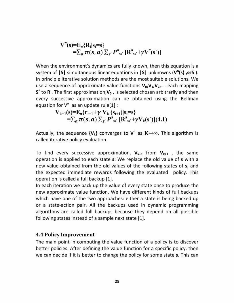
4.3PolicyEvaluationPolicy  evaluation means  to  compute  the  state‐value  function  Vπ  for  an arbitrary policy π . Bellman equation for Vπ(s) is given by:  

25  

                    Vπ(s)=Eπ{Rt|st=s} =∑ ( , )∑ ` a

ss` [Rass`+ Vπ(s`)]

When the environment's dynamics are fully known, then this equation is a system of |S| simultaneous linear equations in |S| unknowns (Vπ(s) ,sϵS ). In principle iterative solution methods are the most suitable solutions. We use a sequence of approximate value functions V0,V1,V2,…. each mapping S+ to R . The first approximation,V0 , is selected chosen arbitrarily and then every  successive  approximation  can  be  obtained  using  the  Bellman equation for Vπ  as an update rule[1] : 

Vk+1(s)=Eπ{rt+1 + Vk (st+1)|st=s} =∑ ( , )∑ ` a

ss` [Rass`+ Vk(s`)](4.1)

Actually,  the  sequence  {Vk}  converges  to Vπ  as K→∞.  This  algorithm  is called iterative policy evaluation.  To  find  every  successive  approximation,  Vk+1  from  Vk+1  ,  the  same operation  is applied to each state s: We replace the old value of s with a new value obtained  from the old values of the  following states of s, and the  expected  immediate  rewards  following  the  evaluated    policy.  This operation is called a full backup [1]. In each iteration we back up the value of every state once to produce the new approximate value function. We have different kinds of full backups which have one of the two approaches: either a state  is being backed up or  a  state‐action  pair.  All  the  backups  used  in  dynamic  programming algorithms  are  called  full  backups  because  they  depend  on  all  possible following states instead of a sample next state [1]. 

4.4PolicyImprovementThe main point  in computing the value function of a policy  is to discover better policies. After defining the value function for a specific policy, then we can decide if it is better to change the policy for some state s. This can 

26  

be  answered  by  checking  whether  Vπ(s)  when  following  the  policy  is greater than or less than. When it is greater, it is better to select a once in s and thereafter follow π than it would be to follow all the time. We would expect it to be better still to select a every time s is encountered, and that the new policy would in fact be a better one overall policies [1].    That this is true is a special case of the policy improvement theorem. Let π and π` be any pair of policies such that, for all sϵS 

Qπ(s,π`(s))≥Vπ(s)

Then we can say that the policy π`is better than or at  least as good as π, because it obtains greater or equal expected return from all states s: 

Vπ`(s)≥ Vπ(s)

4.5DynamicProgrammingEfficiency Dynamic  programming  is  impractical  for  large  problems,  but  when  we compare  to  other methods,  we  can  say  that  dynamic  programming  is indeed extremely efficient. The point to be considered  is that the time  it takes to find an optimal policy  is polynomial  in the number of states and actions.  If  n  and m  denote  the  number  of  states  and  actions,  then  a dynamic  programming  algorithm  takes  a  number  of  computational operations  less than some polynomial  function of n and m. But  it  is sure that  it  can  find  an  optimal  policy  in  polynomial  time  even  though  the number of all policies  is mn . Therefore  it  is exponentially faster than any possible direct search in policy space, because direct search would have to exhaustively examine each policy to provide the same result. We can use also  linear  programming  with  the  advantage  that  its  worst‐case convergence guarantee is better than those of dynamic programming. But linear‐programming methods are somehow impractical at a much smaller number  of  states  .Hence  for  the  largest  problems,  only  dynamic programming methods are feasible [1].  

27  

Dynamic  programming  is  at  some  points  considered  to  be  of  limited applicability  because  of  the  curse  of  dimensionality,  the  fact  that  the number  of  states  often  grows  exponentially  with  the  number  of  state variables. The difficulties arise  in  large state sets, but  these are  inherent difficulties  of  the  problem,  not  of  dynamic  programming  as  a  solution method.  Indeed,  it  is  comparatively better  suited  to handling  very  large state  spaces  than  other  methods  such  as  direct  search  and  linear programming [1].  Dynamic programming methods  can be used with  today's  computers  to solve  problems  with millions  of  states.  Both  policy  iteration  and  value iteration  are widely used,  and  it  is not  clear which  if  either  is better  in general. Those methods converge faster their theoretical worst‐case run‐times,  especially  if  they  are  started with  good  initial  value  functions  or policies [1].                    

 

Thethis 

5.1statTheposinclmetunk First(4X4succnondec 

EachtotaThefour

 code can chapter. 

TheFirstes)  purpose sible stateuded in ththod  in  conown num

t we will d4) system cessfully dn‐decodabloded as sh

Figureh  state  is al decoded  second  for transmitt

Cha

be divided

st Simulat

of  this  sies  in 4X4 ve second sontrast  tomber of sta

describe this consideecoded pae packets hown in [2]

e (8): Retra9X1  row vd packets  four  elemeting anten

apter5:

d  into thre

tion (Calc

mulation virtual MIMsimulation  Monte  Ctes. 

he structurred here wackets  (bufis done  in]. 

ansmissionvector, whfrom eachents  refer nas  in the

28 

TheSim 

ee main pa

culating t

is  to  calcuMO system in order tCarlo  meth

re used  in with a buffffer  limit=n the next 

 of the nonhere  the  fi one of  thto  the  req

e next time

mulations

arts which

thenumb

ulate  the m  ,becauseto apply dyhod  which

this simulfer, where11). The rtime step 

n‐decodabrst  four elhe  four  traquired  rete step. The

s

h will be ex

berofall

total  nume these staynamic proh  can  be 

lation. Virte we save etransmiss until all p

ble signals lements  reansmittingtransmissioe ninth ele

xplained  in

lpossible

mber  of  alates will beogrammingused  with

tual MIMOnumber osion of thepackets are

[2] efer  to  the antennasons  by  theement tells

n 

e

ll e g h 

O f e e 

 

e s. e s 

 

us retr

Thethatwithtran For numfirstthem For the  The Thefollo

1

2

3

if  the  bufransmit the

 action  is t  the correh  value nsmitter.  

every  statmber of zert state or tm is mean

every actinumber o

se actions 

 method uowing step1‐ We star

state. 2‐ When a

move to3‐ When w

one ste

ffer  is  fulle non‐deco

4X1 row vesponding 1  indicat

te  the numros in the sthe all zeroingless. 

 on the nuf ones or t

and states

used to calps: rt from the

a previouslo the next we reach tp to the ne

l  then  weodable pac

vector, whetransmittetes  no  t

mber of psecond pao state the

mber of pransmittin

s can be co

culate num

e first actio

y saved stpossible sthe last nexext action.

29 

e  have  onckets. This 

ere each eer sends aransmissio

ossible actrt of the stere are 24 =

ossible neng antenna

ombined in

mber of sta

on for the 

ate appeatate of thext possible 

nly  action vector is s

element wa packet  inon  from 

tions equatate vecto=16 possib

ext states eas in the co

n a tree as 

ates can be

first state

rs again ore correspone state of a

or  on  timshown in fi

with value n  this  timethe  corr

als 2n wher. For examle actions 

equals 2m worrespondi

shown in f

e describe

 and save 

r the buffending actioan action w

me  slot  togure: 

 1  indicatese step, andresponding

re n  is  themple in thebut one o

where m isng action.

figure (9):

d in by the

every new

er is full weon. we go back

o 

s d g 

e e f 

s 

e 

w 

e 

k 

 

4

UsinMIM 

5.2Thethe statUsinthro 

4‐ The tota(zero st

ng  the  firsMO system

TheSeco purpose opossible ate, which hng  this  taboughput. 

al numberate) during

Figure (9

st  simulatim with buff

ondSimulof this simctions for has  the higble  in choo

r of states ig going ba

9): The tree

on  the  toter limit=11

lation(Crmulation  is each stategher expeosing  the a

30 

is achievedck through

e of the act 

tal  numbe1is: (45873

reatinglooto create e. It containcted  rewaaction  for 

d when weh this tree.

tions and s

er  of  state3 states). 

okuptabla  lookup tns also therd among every  stat

e reach the. 

states 

es  in  this  4

leforallstable whice best actio all possibte will ma

e first state

4X4  virtua

states)ch containson for eachble actionsaximize  the

e 

 

l 

s h s. e 

31  

First, the value of each state is calculated based on Bellman equation in a recursive approach .The value of each state equals the sum of the possible next states multiplied by the probability of having these next states. These  transition  probabilities  are  the  result  of  the  HSA  algorithm  for determining the decoding order .This algorithm is explained in [2]. After calculating the value of each state we can determine the best action for this state, which depends on the possible next states and the transition probabilities.  To calculate the value of each state we need the value of all possible next states which will be calculated depending on the end states. An end  state has no  required  retransmissions;  therefore  it has a  reward equals the number of decoded packets. Furthermore it has a value of zero because such state  is the end of an episode. We need also the Transition probability  matrix  A  ,in  which  1i ja −  is  the  probability  that  we  need  to retransmit with i antennas after transmitting with j antennas  

 0.8562 0.6608 0.3887 0.10620.1438 0.3186 0.5206 0.6081

0 0.0206 0.0877 0.26400 0 0.003 0.02120 0 0 0.00044

⎡ ⎤⎢ ⎥⎢ ⎥⎢ ⎥=⎢ ⎥⎢ ⎥⎢ ⎥⎣ ⎦

A 

  Figure [10] shows the approach used to apply Bellman equation on (2X2) virtual MIMO system .The purpose of this figure is only to explain how the value of each state  is calculated.  In  this  figure Sij  : The  jth possible next state  of  the  ith  action  .To  calculate  the  value  of  the  state  we  apply Bellman equation depending on the value of the possible next states. The next state is either an end state with immediate reward or a normal state so we need to wait  for the  following states to calculate the value of this 

 

statevethe  

5.3TheprevHASexp

Simtranmes

te. After  firy possiblelookup tab

ThePerf code of thvious  simuS  Heuristiclained in [2

ulation shnsmitting  assages. 

nding  the e action  foble.  

Figure

formancehe performulation  andc  Search  A2]. 

ows the oantennas 

value of aor any stat

e (10): calc

Testmance testd  transitioAlgorithm

ptimal polwhich  in  t

32 

all  states, te  .This  is 

culating the

t exploits ton  probabifor  this  4

 licy depenturn  incre

we can cathe appro

e state val

the lookupility matrix4X4  system

ds on redeases  the 

alculate  thoach used 

ue 

p table creax  resultingm.  This  al

ucing the number  o

he value oin building

ated in theg  from  thegorithm  is

number oof  decoded

f g 

 

 

e e s 

f d 

 

Figustarand

 ThewhiactiFigu100 

ure  [11]  shrt from the wait for th

  achievabch  is higheon for eacure  [10]  s,000 Episo

hows one e initial stahe respons

Figure (1

le  througher than oth state.  shows  theodes.  

specific epate and these from th

11): One ep

hput  is  87her policie

e  rate  of 

33 

pisode of  ten choose e system w

 

pisode of th

7.7%  for  thes because

successfu

the  transmthe best awhich is th

he transm

his  4X4  vie we are a

ully  decod

mission,  inaction for ee next stat

ission 

rtual MIMlways usin

ded  signal

 which weevery statete. 

 

MO  systemng the best

ls  through

e e 

, t 

h 

 

 

 

 

 

 

 

 

Figure ((12): The th

34 

hroughput

t of the sysstem 

35  

ConclusionandFutureWorkIn  this  project WSN  with  (4X4)  antennas  has  been  studied  to  find  all possible states which describe  the status of  the decoding process at any time step.  The reason for determining the number of states is to employ DP Dynamic Programming  to  maximize  the  throughput  taking  into  account  that Dynamic  Programming  requires  finding  all  possible  states  to  yield  the optimum policy which results in a higher complexity.  Simulations  show  that  the  optimal  policy  is  to  reduce  the  number  of transmitting antenna, consequently the decoding rate  increases to 87.7% which  is higher than the decoding rate of other policies. Even though the ratio of decoded messages is increased, this does not mean that the data rate  is  increased since reducing the number of transmitting antennas will reduce the data rate.   Concerning  the  future work,  the aforementioned application of dynamic programming does not take  into account the time required  for decoding because  it deals only with maximizing the number of decoded messages. Therefore  it  makes  sense  to  search  for  a  compromise  between  the required time and number of decoded packets.  Moreover it is so important to take into account the channel status before searching  for  the optimal policy, because  it  is clear  that  the channel will affect this optimal policy. 

    

 

36  

References 

[1]  Richard  S.  Sutton,  Andrew  G.  Barto:  Reinforcement  learning:  an introduction.  Adaptive  computation  and  machine  learning,  A  Bradford book.MIT Press, Cambridge ,Mass. [u.a.],[repr.]edition,[2004].  [2]  Selig  M.,  Hunziker  T.,  Dahlhaus  D.:  Enhancing  ZF‐SIC  by  selective retransmissions: on algorithms for determining the decoding order, IEEE 73rd  Vehicular  Technology  Conference  (VTC  Spring  2011), Budapest,Hungary,May 2011.  [3]  Sohraby K,Minoli D,Znati T  :Wireless  Sensor Networks:  Technology  , Protocols and applications. Willey 2007.  [4]  Daniele  Puccinelli  ,  Martin  Haenggi.  Wireless  Sensor  Networks: Applications  and  Challenges  of Ubiquitous  Sensing.  IEEE CIRCUITS AND SYSTEMS MAGAZINE, THIRD QUARTER 2005.  [5] Ajay  Jangra  ,Swati  ,Rich  ,Priyanka. Wireless  Sensor Network  (WSN): Architectural  Design  issues  and  Challenges.  Ajay  Jangra  et  al.  (IJCSE) International Journal on Computer Science and Engineering,2010.  [6]  Schindler, Schulz :Introduction to MIMO. Rohde & Schwarz ,2009.  [7] Ajay  Jangra, Richa, Swati, Priyanka  :Wireless Sensor Network  (WSN): Architectural  Design  issues  and  Challenges.  Ajay  Jangra  et  al.  /  (IJCSE) International Journal on Computer Science and Engineering,2010.   [8] Kermoal,  Schumacher, Mogensen,  Frederiksen  :A  Stochastic MIMO Radio  Channel Model With  Experimental Validation.  IEEE  JOURNAL ON SELECTED AREAS IN COMMUNICATIONS, August 2002.  [9] Mohinder Jankiraman. Space‐Time Codes and MIMO Systems. London. 

37  

ListofFigures 

Figure [1]: Wireless sensor network 

Figure [2]: WSN node components  Figure [3]: MIMO system architecture  

Figure [4]: Different combining methods at the receiver  Figure [5]: Beamforming in multiple antenna system  Figure [6]: Reinforcement learning framework   Figure [7]: The backup diagram  Figure [8]: Retransmission of the non‐decodable signals   Figure [9]: The tree of the actions and states  Figure [10]: Calculating the state value  Figure [11]: One episode of the transmission  Figure [12]: The throughput of the system        

 

38  

Appendix

AppendixA:MATLABcodeforfindingallpossiblestatesinWSNclc clear % The transition probability matrix after simulating the channel transition=[0.856222 0.660829 0.388689/2 0.106165; 0.143778 0.318576 0.520649/3 0.60813/4; 0.0 0.020595 0.087665/3 0.264028/6; 0.0 0.0 0.002997 0.02123/4; 0.0 0.0 0.0 4.47E-4]; w =[0 0 0 0];%number of decoded packets until now status =[0 0 0 0];%required retransmission t =[0 0 0 1];%action d =[0 0 0 0];%The decoded packets after the action lev =1; loop=0; value=0; bufferlimit=12; bufferflag=0; secondflag=0; %levlimit=10; number_of_states=1; buffer = 0; state=[w status secondflag]; line =zeros(200,9); buffer_status=zeros(200,1); allstates=zeros(100000,10); allstates(1,:)=[0 0 0 0 0 0 0 0 0 0]; index=0; while (max(t~=[2 2 2 2]))| (lev>1) w=w+t.*d ;% change decoded packets according to the action and the decoded packets status=xor(t,d);%change required retransmissions line(lev,1:4)=t;%save action lev=lev+1; buffer=sum(w);%calculate the number of messages in the buffer buffer_status(lev)=buffer; %Checking if the number exceeds the buffer limit if buffer > bufferlimit bufferflag=1;

39  

end if bufferflag==1 secondflag=1; end state=[w status secondflag];% The state line(lev,:)=state;%save the state %Check if this state is new index=find(ismember(allstates(:,1:9),state,'rows'),1); % increase the number of states if isempty(index) number_of_states=number_of_states+1; allstates(number_of_states,1:9)=state; loop=0; else loop=1; end %Check if we have an end state if(secondflag==1)|(max(status)==0|loop==1) bufferflag=0; secondflag=0; %assigning the reward according to the state value=0; if(max(status)==0) value=sum(w); elseif secondflag==1 value=0; elseif(loop==1& max(d)>0) value=allstates(index,10); elseif loop==1 value=0; end if loop==0 allstates(find(ismember(allstates(:,1:9),state,'rows'),1),10)=value; end %applying Bellman Equation if(lev>2)

40  

i=find(ismember(allstates(:,1:9),line(lev-2,1:9),'rows'),1); allstates(i,10)=allstates(i,10)+value*transition(sum(status)+1,sum(line(lev-1,1:4))); end w=w-t.*d ;%go back to the next decoding possibility for this action lev=lev-1; if lev==1 buffer=0; else buffer=buffer_status(lev-1); end d=nextd(t,d); while (t==[2 2 2 2])|(d==[2 2 2 2]) %Check if this is the last possible state for this action if d==[2 2 2 2] if lev ==1 t=nextt(t,[ 0 0 0 0]); d=[0 0 0 0]; continue; else t=nextt(t,line(lev-1,5:8)); d=[0 0 0 0]; end end %Check if this is the last possible action if t==[2 2 2 2] %go to the next possible action lev=lev-1; if lev==0 break; end % calculating the value of the previous state if (lev>2) jj=find(ismember(allstates(:,1:9),line(lev-2,1:9),'rows'),1); allstates(i,10)= allstates(i,10)/sum(line(lev+1,1:4))); allstates(jj,10)=allstates(jj,10)+allstates(i,10)*transition(sum(line(lev,5:8))+1,sum(line(lev-1,1:4)));

41  

end % choosing the next decoding state lev=lev-1; t=line(lev,1:4); d=xor(line(lev,1:4),line(lev+1,5:8)); if lev ==1 buffer=0; else buffer=buffer_status(lev-1); end w=w-t.*d ; d=nextd(t,d); end end continue; end t=status; lev=lev+1; d=[0 0 0 0]; end

 

42  

AppendixB:MATLABcodeforfindingtheoptimalpolicy(Creatinglookuptable)

clc clear load states_values.mat number_of_best=0; value=0; best_action=zeros(1,5); current_state=zeros(1,9); states=zeros(16,10); actions=zeros(15,5); corres_actions=zeros(number_of_states,16); allstates(:,10)=0; % calculate the value of each action for every state to decide which is the % best action for iii=2:number_of_states current_state=allstates(iii,1:9); if max(current_state(5:8))==0 continue; end % calculate the value of each action for this state for ii=1:2^(4-(sum(current_state(5:8)))) if(ii==1) actions(ii,1:4)=current_state(5:8); else actions(ii,1:4)=nextt(actions(ii-1,1:4),current_state(5:8)); end % call the values of all possible following states for this action for jj=1:2^(sum(actions(ii,1:4))) if jj==1 states(jj,1:4)=current_state(1:4); states(jj,5:8)=actions(ii,1:4); d=[0 0 0 0]; else d=nextd(actions(ii,1:4),d); states(jj,1:4)=current_state(1:4)+actions(ii,1:4).*d ; states(jj,5:8)=xor(actions(ii,1:4),d); end if sum(states(jj,1:4))> bufferlimit

43  

states(jj,9)=1; else states(jj,9)=0; end states(jj,10)=allstates(find(ismember(allstates(:,1:9),states(jj,1:9),'rows'),1),10); actions(ii,5)=actions(ii,5)+states(jj,10)*transition(sum(states(jj,5:8))+1,sum(actions(ii,1:4))) ; end corres_actions(iii,ii)=actions(ii,5); end if min(current_state(5:8))==1 corres_actions(iii,16)=1; else % decide which is the best action allstates(iii,10)=sum(corres_actions(iii,:))/ii; [value,number_of_best]=max(corres_actions(iii,:)); corres_actions(iii,16)=number_of_best; end end

  

44  

AppendixC:PerformancetestMatlabcode  

clc clear load lookup.mat current_state=zeros(1,9); next_state=zeros(1,9); best_action=zeros(1,4); decoded_action=zeros(1,4); iteration=1; transmitted=0; rate=zeros(1,100000); finalrate=zeros(1,100000); value=0; invalue=0; tdB = -3; t = 10^(tdB/10); rate=0; for jj=1:100000 % Restart if all packets are decoded while(secondflag==0) if(max(current_state(5:8))==0& iteration>1) break; end %Find the state in the lookup table ii=find(ismember(allstates(:,1:9),current_state),1); if iteration==1 best_action=[0 0 1 1]; else best_action=current_state(5:8); %find the best action from the lookup table [value,invalue]=max(corres_actions(ii,:)); for iii=2:invalue best_action= nextt(best_action,current_state(5:8)); end end transmitted=transmitted+sum(best_action); M=sum(best_action);%The number of transmitting antennas N=4;

45  

clear i H = sqrt(1/N/2)*(randn(N,M)+i*randn(N,M));%The channel [max_val_HSA,best_path_HSA,Q,R] = HSA(H,t);%Applying HSA decoding order decoded_action=[0 0 0 0]; if max_val_HSA>0 for ii=1:4 if(best_action(ii)==1) decoded_action(ii)=1; max_val_HSA=max_val_HSA-1; if max_val_HSA<0 decoded_action(ii)=0; end end end end %Find the next state next_state(1:4)=current_state(1:4)+decoded_action; next_state(5:8)=xor(best_action,decoded_action); if sum(next_state(1:4))>bufferlimit next_state(9)=1; else next_state(9)=0; end second_flag=and(current_state(9),next_state(9)); current_state=next_state; iteration=iteration+1; end %calculate the rate if max(current_state(5:8))==0 rate(jj)=sum(current_state(1:4))/transmitted; else rate(jj)=0 end transmitted=0; iteration=1; current_state=zeros(1,9); %calculate the total rate finalrate(jj)=sum(rate)/jj;

46  

end plot(finalrate) axis([0 100000 0.6 1])