javascript data structures and algorithms · therefore, this book aims to teach data structure and...
TRANSCRIPT

JavaScript Data Structures and Algorithms
An Introduction to Understanding and Implementing Core Data Structure and Algorithm Fundamentals—Sammie Bae
www.allitebooks.com

JavaScript Data Structures and Algorithms
An Introduction to Understanding and Implementing Core Data
Structure and Algorithm Fundamentals
Sammie Bae
www.allitebooks.com

JavaScript Data Structures and Algorithms
ISBN-13 (pbk): 978-1-4842-3987-2 ISBN-13 (electronic): 978-1-4842-3988-9https://doi.org/10.1007/978-1-4842-3988-9
Library of Congress Control Number: 2019930417
Copyright © 2019 by Sammie Bae
This work is subject to copyright. All rights are reserved by the Publisher, whether the whole or part of the material is concerned, specifically the rights of translation, reprinting, reuse of illustrations, recitation, broadcasting, reproduction on microfilms or in any other physical way, and transmission or information storage and retrieval, electronic adaptation, computer software, or by similar or dissimilar methodology now known or hereafter developed.
Trademarked names, logos, and images may appear in this book. Rather than use a trademark symbol with every occurrence of a trademarked name, logo, or image we use the names, logos, and images only in an editorial fashion and to the benefit of the trademark owner, with no intention of infringement of the trademark.
The use in this publication of trade names, trademarks, service marks, and similar terms, even if they are not identified as such, is not to be taken as an expression of opinion as to whether or not they are subject to proprietary rights.
While the advice and information in this book are believed to be true and accurate at the date of publication, neither the authors nor the editors nor the publisher can accept any legal responsibility for any errors or omissions that may be made. The publisher makes no warranty, express or implied, with respect to the material contained herein.
Managing Director, Apress Media LLC: Welmoed SpahrAcquisitions Editor: Louise CorriganDevelopment Editor: Chris NelsonCoordinating Editor: Nancy Chen
Cover designed by eStudioCalamar
Distributed to the book trade worldwide by Springer Science+Business Media New York, 233 Spring Street, 6th Floor, New York, NY 10013. Phone 1-800-SPRINGER, fax (201) 348-4505, e-mail [email protected], or visit www.springeronline.com. Apress Media, LLC is a California LLC and the sole member (owner) is Springer Science + Business Media Finance Inc (SSBM Finance Inc). SSBM Finance Inc is a Delaware corporation.
For information on translations, please e-mail [email protected], or visit www.apress.com/rights-permissions.
Apress titles may be purchased in bulk for academic, corporate, or promotional use. eBook versions and licenses are also available for most titles. For more information, reference our Print and eBook Bulk Sales web page at www.apress.com/bulk-sales.
Any source code or other supplementary material referenced by the author in this book is available to readers on GitHub via the book’s product page, located at www.apress.com/9781484239872. For more detailed information, please visit www.apress.com/source-code.
Printed on acid-free paper
Sammie BaeHamilton, ON, Canada
www.allitebooks.com

This book is dedicated to Dr. Hamid R. Tizhoosh for inspiring me in my studies and to my mother, Min Kyoung Seo, for her
kindness and support.
www.allitebooks.com

v
Table of Contents
Chapter 1: Big-O Notation ����������������������������������������������������������������������������������������� 1Big-O Notation Primer ������������������������������������������������������������������������������������������������������������������� 1
Common Examples ������������������������������������������������������������������������������������������������������������������ 2
Rules of Big-O Notation ����������������������������������������������������������������������������������������������������������������� 4
Coefficient Rule: “Get Rid of Constants” ���������������������������������������������������������������������������������� 5
Sum Rule: “Add Big-Os Up” ����������������������������������������������������������������������������������������������������� 6
Product Rule: “Multiply Big-Os” ���������������������������������������������������������������������������������������������� 7
Polynomial Rule: “Big-O to the Power of k”����������������������������������������������������������������������������� 8
Summary��������������������������������������������������������������������������������������������������������������������������������������� 8
Exercises ��������������������������������������������������������������������������������������������������������������������������������������� 9
Answers ��������������������������������������������������������������������������������������������������������������������������������� 11
Chapter 2: JavaScript: Unique Parts ����������������������������������������������������������������������� 13JavaScript Scope ������������������������������������������������������������������������������������������������������������������������ 13
Global Declaration: Global Scope ������������������������������������������������������������������������������������������� 13
Declaration with var: Functional Scope ��������������������������������������������������������������������������������� 13
Declaration with let: Block Scope ������������������������������������������������������������������������������������������ 15
About the Author �����������������������������������������������������������������������������������������������������xv
About the Technical Reviewer �������������������������������������������������������������������������������xvii
Acknowledgments ��������������������������������������������������������������������������������������������������xix
Introduction ������������������������������������������������������������������������������������������������������������xxi
www.allitebooks.com

vi
Equality and Types ���������������������������������������������������������������������������������������������������������������������� 16
Variable Types ������������������������������������������������������������������������������������������������������������������������ 16
Truthy/Falsey Check �������������������������������������������������������������������������������������������������������������� 17
=== vs == ���������������������������������������������������������������������������������������������������������������������������� 18
Objects ���������������������������������������������������������������������������������������������������������������������������������� 18
Summary������������������������������������������������������������������������������������������������������������������������������������� 20
Chapter 3: JavaScript Numbers ������������������������������������������������������������������������������ 21Number System �������������������������������������������������������������������������������������������������������������������������� 21
JavaScript Number Object ���������������������������������������������������������������������������������������������������������� 23
Integer Rounding ������������������������������������������������������������������������������������������������������������������� 23
Number�EPSILON ������������������������������������������������������������������������������������������������������������������� 24
Maximums ����������������������������������������������������������������������������������������������������������������������������� 24
Minimums ������������������������������������������������������������������������������������������������������������������������������ 25
Size Summary ����������������������������������������������������������������������������������������������������������������������� 26
Number Algorithms ���������������������������������������������������������������������������������������������������������������� 26
Prime Factorization ��������������������������������������������������������������������������������������������������������������� 28
Random Number Generator �������������������������������������������������������������������������������������������������������� 29
Exercises ������������������������������������������������������������������������������������������������������������������������������������� 29
Summary������������������������������������������������������������������������������������������������������������������������������������� 34
Chapter 4: JavaScript Strings ��������������������������������������������������������������������������������� 35JavaScript String Primitive ��������������������������������������������������������������������������������������������������������� 35
String Access ������������������������������������������������������������������������������������������������������������������������� 35
String Comparison ����������������������������������������������������������������������������������������������������������������� 36
String Search ������������������������������������������������������������������������������������������������������������������������� 36
String Decomposition ������������������������������������������������������������������������������������������������������������ 38
String Replace ����������������������������������������������������������������������������������������������������������������������� 38
Regular Expressions ������������������������������������������������������������������������������������������������������������������� 38
Basic Regex ��������������������������������������������������������������������������������������������������������������������������� 39
Commonly Used Regexes ������������������������������������������������������������������������������������������������������ 39
Encoding ������������������������������������������������������������������������������������������������������������������������������������� 41
Base64 Encoding ������������������������������������������������������������������������������������������������������������������� 42
Table of ConTenTs
vii
String Shortening ������������������������������������������������������������������������������������������������������������������������ 43
Encryption ����������������������������������������������������������������������������������������������������������������������������������� 45
RSA Encryption ���������������������������������������������������������������������������������������������������������������������� 46
Summary ������������������������������������������������������������������������������������������������������������������������������� 50
Chapter 5: JavaScript Arrays���������������������������������������������������������������������������������� 53Introducing Arrays ����������������������������������������������������������������������������������������������������������������������� 53
Insertion �������������������������������������������������������������������������������������������������������������������������������� 53
Deletion ��������������������������������������������������������������������������������������������������������������������������������� 54
Access ����������������������������������������������������������������������������������������������������������������������������������� 54
Iteration ��������������������������������������������������������������������������������������������������������������������������������������� 54
for (Variables; Condition; Modification) ��������������������������������������������������������������������������������� 55
for ( in ) ���������������������������������������������������������������������������������������������������������������������������������� 56
for ( of ) ���������������������������������������������������������������������������������������������������������������������������������� 56
forEach( ) �������������������������������������������������������������������������������������������������������������������������������� 56
Helper Functions ������������������������������������������������������������������������������������������������������������������������� 57
�slice(begin,end) �������������������������������������������������������������������������������������������������������������������� 57
� splice(begin,size,element1,element2…) ������������������������������������������������������������������������������ 58
� concat() ��������������������������������������������������������������������������������������������������������������������������������� 59
� length Property ��������������������������������������������������������������������������������������������������������������������� 59
Spread Operator �������������������������������������������������������������������������������������������������������������������� 60
Exercises ������������������������������������������������������������������������������������������������������������������������������������� 60
JavaScript Functional Array Methods ����������������������������������������������������������������������������������������� 67
Map���������������������������������������������������������������������������������������������������������������������������������������� 67
Filter �������������������������������������������������������������������������������������������������������������������������������������� 68
Reduce ���������������������������������������������������������������������������������������������������������������������������������� 68
Multidimensional Arrays ������������������������������������������������������������������������������������������������������������� 68
Exercises ������������������������������������������������������������������������������������������������������������������������������������� 71
Summary������������������������������������������������������������������������������������������������������������������������������������� 81
Table of ConTenTs

viii
Chapter 6: JavaScript Objects �������������������������������������������������������������������������������� 83JavaScript Object Property ��������������������������������������������������������������������������������������������������������� 83
Prototypal Inheritance ����������������������������������������������������������������������������������������������������������������� 84
Constructor and Variables ����������������������������������������������������������������������������������������������������������� 85
Summary������������������������������������������������������������������������������������������������������������������������������������� 86
Exercises ������������������������������������������������������������������������������������������������������������������������������������� 87
Chapter 7: JavaScript Memory Management ��������������������������������������������������������� 89Memory Leaks ���������������������������������������������������������������������������������������������������������������������������� 89
Reference to an Object ���������������������������������������������������������������������������������������������������������� 89
Leaking DOM ������������������������������������������������������������������������������������������������������������������������� 90
Global window Object ������������������������������������������������������������������������������������������������������������ 91
Limiting Object References ��������������������������������������������������������������������������������������������������� 92
The delete Operator ��������������������������������������������������������������������������������������������������������������� 92
Summary������������������������������������������������������������������������������������������������������������������������������������� 93
Exercises ������������������������������������������������������������������������������������������������������������������������������������� 93
Chapter 8: Recursion ���������������������������������������������������������������������������������������������� 99Introducing Recursion ����������������������������������������������������������������������������������������������������������������� 99
Rules of Recursion �������������������������������������������������������������������������������������������������������������������� 100
Base Case ���������������������������������������������������������������������������������������������������������������������������� 100
Divide-and-Conquer Method ����������������������������������������������������������������������������������������������� 101
Classic Example: Fibonacci Sequence �������������������������������������������������������������������������������� 101
Fibonacci Sequence: Tail Recursion ������������������������������������������������������������������������������������ 102
Pascal’s Triangle ������������������������������������������������������������������������������������������������������������������ 103
Big-O for Recursion ������������������������������������������������������������������������������������������������������������������� 105
Recurrence Relations ���������������������������������������������������������������������������������������������������������� 105
Master Theorem ������������������������������������������������������������������������������������������������������������������ 106
Recursive Call Stack Memory ��������������������������������������������������������������������������������������������������� 107
Summary����������������������������������������������������������������������������������������������������������������������������������� 109
Exercises ����������������������������������������������������������������������������������������������������������������������������������� 109
Table of ConTenTs

ix
Chapter 9: Sets ����������������������������������������������������������������������������������������������������� 117Introducing Sets ������������������������������������������������������������������������������������������������������������������������ 117
Set Operations �������������������������������������������������������������������������������������������������������������������������� 117
Insertion ������������������������������������������������������������������������������������������������������������������������������ 118
Deletion ������������������������������������������������������������������������������������������������������������������������������� 118
Contains ������������������������������������������������������������������������������������������������������������������������������� 118
Other Utility Functions��������������������������������������������������������������������������������������������������������������� 119
Intersection �������������������������������������������������������������������������������������������������������������������������� 119
isSuperSet ��������������������������������������������������������������������������������������������������������������������������� 119
Union ����������������������������������������������������������������������������������������������������������������������������������� 120
Difference ���������������������������������������������������������������������������������������������������������������������������� 120
Summary����������������������������������������������������������������������������������������������������������������������������������� 121
Exercises ����������������������������������������������������������������������������������������������������������������������������������� 122
Chapter 10: Searching and Sorting ���������������������������������������������������������������������� 125Searching ���������������������������������������������������������������������������������������������������������������������������������� 125
Linear Search ���������������������������������������������������������������������������������������������������������������������� 125
Binary Search ���������������������������������������������������������������������������������������������������������������������� 127
Sorting �������������������������������������������������������������������������������������������������������������������������������������� 129
Bubble Sort �������������������������������������������������������������������������������������������������������������������������� 129
Selection Sort ���������������������������������������������������������������������������������������������������������������������� 131
Insertion Sort ����������������������������������������������������������������������������������������������������������������������� 132
Quicksort ����������������������������������������������������������������������������������������������������������������������������� 134
Quickselect �������������������������������������������������������������������������������������������������������������������������� 137
Mergesort ���������������������������������������������������������������������������������������������������������������������������� 138
Count Sort ���������������������������������������������������������������������������������������������������������������������������� 140
JavaScript’s Built-in Sort ����������������������������������������������������������������������������������������������������� 141
Summary����������������������������������������������������������������������������������������������������������������������������������� 142
Exercises ����������������������������������������������������������������������������������������������������������������������������������� 143
Table of ConTenTs

x
Chapter 11: Hash Tables ��������������������������������������������������������������������������������������� 151Introducing Hash Tables ������������������������������������������������������������������������������������������������������������ 151
Hashing Techniques ������������������������������������������������������������������������������������������������������������������ 152
Prime Number Hashing ������������������������������������������������������������������������������������������������������� 152
Probing �������������������������������������������������������������������������������������������������������������������������������� 154
Rehashing/Double-Hashing ������������������������������������������������������������������������������������������������� 155
Hash Table Implementation ������������������������������������������������������������������������������������������������������� 156
Using Linear Probing ����������������������������������������������������������������������������������������������������������� 156
Using Quadratic Probing ������������������������������������������������������������������������������������������������������ 158
Using Double-Hashing with Linear Probing ������������������������������������������������������������������������� 160
Summary����������������������������������������������������������������������������������������������������������������������������������� 161
Chapter 12: Stacks and Queues ���������������������������������������������������������������������������� 163Stacks ��������������������������������������������������������������������������������������������������������������������������������������� 163
Peek ������������������������������������������������������������������������������������������������������������������������������������� 165
Insertion ������������������������������������������������������������������������������������������������������������������������������ 165
Deletion ������������������������������������������������������������������������������������������������������������������������������� 166
Access ��������������������������������������������������������������������������������������������������������������������������������� 166
Search ��������������������������������������������������������������������������������������������������������������������������������� 167
Queues �������������������������������������������������������������������������������������������������������������������������������������� 167
Peek ������������������������������������������������������������������������������������������������������������������������������������� 169
Insertion ������������������������������������������������������������������������������������������������������������������������������ 169
Deletion ������������������������������������������������������������������������������������������������������������������������������� 169
Access ��������������������������������������������������������������������������������������������������������������������������������� 170
Search ��������������������������������������������������������������������������������������������������������������������������������� 171
Summary����������������������������������������������������������������������������������������������������������������������������������� 171
Exercises ����������������������������������������������������������������������������������������������������������������������������������� 172
Chapter 13: Linked Lists ��������������������������������������������������������������������������������������� 179Singly Linked Lists �������������������������������������������������������������������������������������������������������������������� 179
Insertion ������������������������������������������������������������������������������������������������������������������������������ 180
Deletion by Value ����������������������������������������������������������������������������������������������������������������� 181
Table of ConTenTs

xi
Deletion at the Head ������������������������������������������������������������������������������������������������������������ 182
Search ��������������������������������������������������������������������������������������������������������������������������������� 183
Doubly Linked Lists ������������������������������������������������������������������������������������������������������������������� 184
Insertion at the Head ����������������������������������������������������������������������������������������������������������� 185
Insertion at the Tail �������������������������������������������������������������������������������������������������������������� 185
Deletion at the Head ������������������������������������������������������������������������������������������������������������ 186
Deletion at the Tail ��������������������������������������������������������������������������������������������������������������� 187
Search ��������������������������������������������������������������������������������������������������������������������������������� 188
Summary����������������������������������������������������������������������������������������������������������������������������������� 189
Exercises ����������������������������������������������������������������������������������������������������������������������������������� 190
Chapter 14: Caching ��������������������������������������������������������������������������������������������� 193Understanding Caching ������������������������������������������������������������������������������������������������������������� 193
Least Frequently Used Caching ������������������������������������������������������������������������������������������������� 194
Least Recently Used Caching ���������������������������������������������������������������������������������������������������� 199
Summary����������������������������������������������������������������������������������������������������������������������������������� 203
Chapter 15: Trees �������������������������������������������������������������������������������������������������� 205General Tree Structure �������������������������������������������������������������������������������������������������������������� 205
Binary Trees ������������������������������������������������������������������������������������������������������������������������������ 206
Tree Traversal ���������������������������������������������������������������������������������������������������������������������������� 207
Pre-order Traversal �������������������������������������������������������������������������������������������������������������� 207
In-Order Traversal ���������������������������������������������������������������������������������������������������������������� 209
Post-order Traversal ������������������������������������������������������������������������������������������������������������ 211
Level-Order Traversal ���������������������������������������������������������������������������������������������������������� 212
Tree Traversal Summary ������������������������������������������������������������������������������������������������������ 214
Binary Search Trees ������������������������������������������������������������������������������������������������������������������ 214
Insertion ������������������������������������������������������������������������������������������������������������������������������ 216
Deletion ������������������������������������������������������������������������������������������������������������������������������� 218
Search ��������������������������������������������������������������������������������������������������������������������������������� 220
Table of ConTenTs

xii
AVL Trees ����������������������������������������������������������������������������������������������������������������������������������� 221
Single Rotation �������������������������������������������������������������������������������������������������������������������� 221
Double Rotation ������������������������������������������������������������������������������������������������������������������� 225
Balancing the Tree ��������������������������������������������������������������������������������������������������������������� 228
Insertion ������������������������������������������������������������������������������������������������������������������������������ 229
Putting It All Together: AVL Tree Example ����������������������������������������������������������������������������� 231
Summary����������������������������������������������������������������������������������������������������������������������������������� 234
Exercises ����������������������������������������������������������������������������������������������������������������������������������� 234
Chapter 16: Heaps ������������������������������������������������������������������������������������������������ 245Understanding Heaps ���������������������������������������������������������������������������������������������������������������� 245
Max-Heap ���������������������������������������������������������������������������������������������������������������������������� 246
Min-Heap ����������������������������������������������������������������������������������������������������������������������������� 247
Binary Heap Array Index Structure �������������������������������������������������������������������������������������������� 248
Percolation: Bubbling Up and Down ������������������������������������������������������������������������������������ 250
Implementing Percolation���������������������������������������������������������������������������������������������������� 253
Max-Heap Example ������������������������������������������������������������������������������������������������������������� 254
Min-Heap Complete Implementation ���������������������������������������������������������������������������������������� 258
Max-Heap Complete Implementation ��������������������������������������������������������������������������������������� 259
Heap Sort ���������������������������������������������������������������������������������������������������������������������������������� 261
Ascending-Order Sort (Min-Heap) ��������������������������������������������������������������������������������������� 261
Descending-Order Sort (Max-Heap) ������������������������������������������������������������������������������������ 264
Summary����������������������������������������������������������������������������������������������������������������������������������� 267
Exercises ����������������������������������������������������������������������������������������������������������������������������������� 268
Chapter 17: Graphs ����������������������������������������������������������������������������������������������� 273Graph Basics ����������������������������������������������������������������������������������������������������������������������������� 273
Undirected Graphs �������������������������������������������������������������������������������������������������������������������� 277
Adding Edges and Vertices �������������������������������������������������������������������������������������������������� 279
Removing Edges and Vertices ��������������������������������������������������������������������������������������������� 280
Directed Graphs ������������������������������������������������������������������������������������������������������������������������ 282
Table of ConTenTs
xiii
Graph Traversal ������������������������������������������������������������������������������������������������������������������������� 285
Breadth-First Search ����������������������������������������������������������������������������������������������������������� 286
Depth-First Search �������������������������������������������������������������������������������������������������������������� 289
Weighted Graphs and Shortest Path ����������������������������������������������������������������������������������������� 293
Graphs with Weighted Edges ����������������������������������������������������������������������������������������������� 293
Dijkstra’s Algorithm: Shortest Path �������������������������������������������������������������������������������������� 294
Topological Sort ������������������������������������������������������������������������������������������������������������������������ 298
Summary����������������������������������������������������������������������������������������������������������������������������������� 300
Chapter 18: Advanced Strings ������������������������������������������������������������������������������ 303Trie (Prefix Tree) ������������������������������������������������������������������������������������������������������������������������ 303
Boyer–Moore String Search ������������������������������������������������������������������������������������������������������ 307
Knuth–Morris–Pratt String Search �������������������������������������������������������������������������������������������� 311
Rabin–Karp Search ������������������������������������������������������������������������������������������������������������������� 316
The Rabin Fingerprint ���������������������������������������������������������������������������������������������������������� 316
Applications in Real Life ������������������������������������������������������������������������������������������������������ 319
Summary����������������������������������������������������������������������������������������������������������������������������������� 320
Chapter 19: Dynamic Programming ��������������������������������������������������������������������� 321Motivations for Dynamic Programming������������������������������������������������������������������������������������� 321
Rules of Dynamic Programming ����������������������������������������������������������������������������������������������� 323
Overlapping Subproblems ��������������������������������������������������������������������������������������������������� 323
Optimal Substructure ���������������������������������������������������������������������������������������������������������� 323
Example: Ways to Cover Steps �������������������������������������������������������������������������������������������� 323
Classical Dynamic Programming Examples ������������������������������������������������������������������������������ 325
The Knapsack Problem �������������������������������������������������������������������������������������������������������� 325
Longest Common Subsequence ������������������������������������������������������������������������������������������ 328
Coin Change ������������������������������������������������������������������������������������������������������������������������ 330
Edit (Levenshtein) Distance ������������������������������������������������������������������������������������������������� 334
Summary����������������������������������������������������������������������������������������������������������������������������������� 338
Table of ConTenTs

xiv
Chapter 20: Bit Manipulation �������������������������������������������������������������������������������� 339Bitwise Operators ��������������������������������������������������������������������������������������������������������������������� 339
AND �������������������������������������������������������������������������������������������������������������������������������������� 340
OR ���������������������������������������������������������������������������������������������������������������������������������������� 340
XOR �������������������������������������������������������������������������������������������������������������������������������������� 341
NOT �������������������������������������������������������������������������������������������������������������������������������������� 341
Left Shift ������������������������������������������������������������������������������������������������������������������������������ 342
Right Shift ���������������������������������������������������������������������������������������������������������������������������� 342
Zero-Fill Right Shift ������������������������������������������������������������������������������������������������������������� 343
Number Operations ������������������������������������������������������������������������������������������������������������������� 343
Addition ������������������������������������������������������������������������������������������������������������������������������� 343
Subtraction �������������������������������������������������������������������������������������������������������������������������� 344
Multiplication ����������������������������������������������������������������������������������������������������������������������� 345
Division �������������������������������������������������������������������������������������������������������������������������������� 347
Summary����������������������������������������������������������������������������������������������������������������������������������� 349
Index ��������������������������������������������������������������������������������������������������������������������� 351
Table of ConTenTs
xv
About the Author
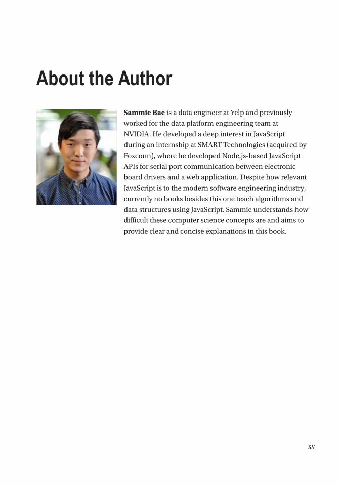
Sammie Bae is a data engineer at Yelp and previously
worked for the data platform engineering team at
NVIDIA. He developed a deep interest in JavaScript
during an internship at SMART Technologies (acquired by
Foxconn), where he developed Node.js-based JavaScript
APIs for serial port communication between electronic
board drivers and a web application. Despite how relevant
JavaScript is to the modern software engineering industry,
currently no books besides this one teach algorithms and
data structures using JavaScript. Sammie understands how
difficult these computer science concepts are and aims to
provide clear and concise explanations in this book.

xvii
About the Technical Reviewer
Phil Nash is a developer evangelist for Twilio, serving
developer communities in London and all over the world.
He is a Ruby, JavaScript, and Swift developer; Google
Developers Expert; blogger; speaker; and occasional brewer.
He can be found hanging out at meetups and conferences,
playing with new technologies and APIs, or writing open
source code.

xix
Acknowledgments
Thank you, Phil Nash, for the valuable feedback that helped me improve the technical
content of this book with clear explanations and concise code.
Special thanks to the Apress team. This includes James Markham, Nancy Chen, Jade
Scard, and Chris Nelson. Finally, I want to thank Steve Anglin for reaching out to me to
publish with Apress.

xxi
Introduction
The motivation for writing this book was the lack of resources available about data
structures and algorithms written in JavaScript. This was strange to me because
today many of the job opportunities for software development require knowledge of
JavaScript; it is the only language that can be used to write the entire stack, including the
front-end, mobile (native and hybrid) platforms, and back-end. It is crucial for JavaScript
developers to understand how data structures work and how to design algorithms to
build applications.
Therefore, this book aims to teach data structure and algorithm concepts from
computer science for JavaScript rather than for the more typical Java or C++. Because
JavaScript follows the prototypal inheritance pattern, unlike Java and C++ (which follow
the inheritance pattern), there are some changes in writing data structures in JavaScript.
The classical inheritance pattern allows inheritance by creating a blueprint- like form
that objects follow during inheritance. However, the prototypal inheritance pattern
means copying the objects and changing their properties.
This book first covers fundamental mathematics for Big-O analysis and then lays out
the basic JavaScript foundations, such as primitive objects and types. Then, this book
covers implementations and algorithms for fundamental data structures such as linked
lists, stacks, trees, heaps, and graphs. Finally, more advanced topics such as efficient
string search algorithms, caching algorithms, and dynamic programming problems are
explored in great detail.

1© Sammie Bae 2019 S. Bae, JavaScript Data Structures and Algorithms, https://doi.org/10.1007/978-1-4842-3988-9_1
CHAPTER 1
Big-O Notation
O(1) is holy.
—Hamid Tizhoosh
Before learning how to implement algorithms, you should understand how to analyze
the effectiveness of them. This chapter will focus on the concept of Big-O notation for
time and algorithmic space complexity analysis. By the end of this chapter, you will
understand how to analyze an implementation of an algorithm with respect to both time
(execution time) and space (memory consumed).
Big-O Notation PrimerThe Big-O notation measures the worst-case complexity of an algorithm. In Big-O
notation, n represents the number of inputs. The question asked with Big-O is the
following: “What will happen as n approaches infinity?”
When you implement an algorithm, Big-O notation is important because it tells you
how efficient the algorithm is. Figure 1-1 shows some common Big-O notations.

2
The following sections illustrate these common time complexities with some simple
examples.
Common ExamplesO(1) does not change with respect to input space. Hence, O(1) is referred to as being
constant time. An example of an O(1) algorithm is accessing an item in the array by its
index. O(n) is linear time and applies to algorithms that must do n operations in the
worst-case scenario.
An example of an O(n) algorithm is printing numbers from 0 to n-1, as shown here:
1 function exampleLinear(n) {
2 for (var i = 0 ; i < n; i++ ) {
Figure 1-1. Common Big-O complexities
Chapter 1 Big-O NOtatiON

3
3 console.log(i);
4 }
5 }
Similarly, O(n2) is quadratic time, and O(n3) is cubic time. Examples of these
complexities are shown here:
1 function exampleQuadratic(n) {
2 for (var i = 0 ; i < n; i++ ) {
3 console.log(i);
4 for (var j = i; j < n; j++ ) {
5 console.log(j);
6 }
7 }
8 }
1 function exampleCubic(n) {
2 for (var i = 0 ; i < n; i++ ) {
3 console.log(i);
4 for (var j = i; j < n; j++ ) {
5 console.log(j);
6 for (var k = j;
j < n; j++ ) {
7 console.log(k);
8 }
9 }
10 }
11 }
Finally, an example algorithm of logarithmic time complexity is printing elements
that are a power of 2 between 2 and n. For example, exampleLogarithmic(10) will print
the following:
2,4,8,16,32,64
Chapter 1 Big-O NOtatiON

4
The efficiency of logarithmic time complexities is apparent with large inputs such
as a million items. Although n is a million, exampleLogarithmic will print only 19
items because log2(1,000,000) = 19.9315686. The code that implements this logarithmic
behavior is as follows:
1 function exampleLogarithmic(n) {
2 for (var i = 2 ; i <= n; i= i*2 ) {
3 console.log(i);
4 }
5 }
Rules of Big-O NotationLet’s represent an algorithm’s complexity as f(n). n represents the number of inputs,
f(n)time represents the time needed, and f(n)space represents the space (additional
memory) needed for the algorithm. The goal of algorithm analysis is to understand the
algorithm’s efficiency by calculating f(n). However, it can be challenging to calculate f(n).
Big-O notation provides some fundamental rules that help developers compute for f(n).
• Coefficient rule: If f(n) is O(g(n)), then kf(n) is O(g(n)), for any
constant k > 0. The first rule is the coefficient rule, which eliminates
coefficients not related to the input size, n. This is because as n
approaches infinity, the other coefficient becomes negligible.
• Sum rule: If f(n) is O(h(n)) and g(n) is O(p(n)), then f(n)+g(n) is
O(h(n)+p(n)). The sum rule simply states that if a resultant time
complexity is a sum of two different time complexities, the resultant
Big-O notation is also the sum of two different Big-O notations.
• Product rule: If f(n) is O(h(n)) and g(n) is O(p(n)), then f(n)g(n) is
O(h(n)p(n)). Similarly, the product rule states that Big-O is multiplied
when the time complexities are multiplied.
• Transitive rule: If f(n) is O(g(n)) and g(n) is O(h(n)), then f(n) is
O(h(n)). The transitive rule is a simple way to state that the same time
complexity has the same Big-O.
Chapter 1 Big-O NOtatiON

5
• Polynomial rule: If f(n) is a polynomial of degree k, then f(n) is
O(nk). Intuitively, the polynomial rule states that polynomial time
complexities have Big-O of the same polynomial degree.
• Log of a power rule: log(nk) is O(log(n)) for any constant k > 0. With
the log of a power rule, constants within a log function are also
ignored in Big-O notation.
Special attention should be paid to the first three rules and the polynomial rule
because they are the most commonly used. I’ll discuss each of those rules in the
following sections.
Coefficient Rule: “Get Rid of Constants”Let’s first review the coefficient rule. This rule is the easiest rule to understand. It simply
requires you to ignore any non-input-size-related constants. Coefficients in Big-O are
negligible with large input sizes. Therefore, this is the most important rule of Big-O
notations.
If f(n) is O(g(n)), then kf(n) is O(g(n)), for any constant k > 0.
This means that both 5f(n) and f(n) have the same Big-O notation of O(f(n)).
Here is an example of a code block with a time complexity of O(n):
1 function a(n){
2 var count =0;
3 for (var i=0;i<n;i++){
4 count+=1;
5 }
6 return count;
7 }
This block of code has f(n) = n. This is because it adds to count n times. Therefore,
this function is O(n) in time complexity:
1 function a(n){
2 var count =0;
3 for (var i=0;i<5*n;i++){
Chapter 1 Big-O NOtatiON

6
4 count+=1;
5 }
6 return count;
7 }
This block has f(n) = 5n. This is because it runs from 0 to 5n. However, the first two
examples both have a Big-O notation of O(n). Simply put, this is because if n is close to
infinity or another large number, those four additional operations are meaningless. It is
going to perform it n times. Any constants are negligible in Big-O notation.
The following code block demonstrates another function with a linear time
complexity but with an additional operation on line 6:
1 function a(n){
2 var count =0;
3 for (var i=0;i<n;i++){
4 count+=1;
5 }
6 count+=3;
7 return count;
8 }
Lastly, this block of code has f(n) = n+1. There is +1 from the last operation
(count+=3). This still has a Big-O notation of O(n). This is because that 1 operation is not
dependent on the input n. As n approaches infinity, it will become negligible.
Sum Rule: “Add Big-Os Up”The sum rule is intuitive to understand; time complexities can be added. Imagine a
master algorithm that involves two other algorithms. The Big-O notation of that master
algorithm is simply the sum of the other two Big-O notations.
If f(n) is O(h(n)) and g(n) is O(p(n)), then f(n)+g(n) is O(h(n)+p(n)).
It is important to remember to apply the coefficient rule after applying this rule.
Chapter 1 Big-O NOtatiON

7
The following code block demonstrates a function with two main loops whose time
complexities must be considered independently and then summed:
1 function a(n){
2 var count =0;
3 for (var i=0;i<n;i++){
4 count+=1;
5 }
6 for (var i=0;i<5*n;i++){
7 count+=1;
8 }
9 return count;
10 }
In this example, line 4 has f(n) = n, and line 7 has f(n) = 5n. This results in 6n.
However, when applying the coefficient rule, the final result is O(n) = n.
Product Rule: “Multiply Big-Os”The product rule simply states how Big-Os can be multiplied.
If f(n) is O(h(n)) and g(n) is O(p(n)), then f(n)g(n) is O(h(n)p(n)).
The following code block demonstrates a function with two nested for loops for
which the product rule is applied:
1 function (n){
2 var count =0;
3 for (var i=0;i<n;i++){
4 count+=1;
5 for (var i=0;i<5*n;i++){
6 count+=1;
7 }
8 }
9 return count;
10 }
Chapter 1 Big-O NOtatiON

8
In this example, f(n) = 5n*n because line 7 runs 5n times for a total of n iterations.
Therefore, this results in a total of 5n2 operations. Applying the coefficient rule, the result
is that O(n)=n2.
Polynomial Rule: “Big-O to the Power of k”The polynomial rule states that polynomial time complexities have a Big-O notation of
the same polynomial degree.
Mathematically, it’s as follows:
If f(n) is a polynomial of degree k, then f(n) is O(nk).
The following code block has only one for loop with quadratic time complexity:
1 function a(n){
2 var count =0;
3 for (var i=0;i<n*n;i++){
4 count+=1;
5 }
6 return count;
7 }
In this example, f(n) = nˆ2 because line 4 runs n*n iterations.
This was a quick overview of the Big-O notation. There is more to come as you
progress through the book.
SummaryBig-O is important for analyzing and comparing the efficiencies of algorithms.
The analysis of Big-O starts by looking at the code and applying the rules to simplify
the Big-O notation. The following are the most often used rules:
• Eliminating coefficients/constants (coefficient rule)
• Adding up Big-Os (sum rule)
• Multiplying Big-Os (product rule)
• Determining the polynomial of the Big-O notation by looking at loops
(polynomial rule)
Chapter 1 Big-O NOtatiON
9
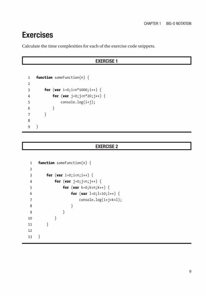
ExercisesCalculate the time complexities for each of the exercise code snippets.
EXERCISE 1
1 function someFunction(n) {
2
3 for (var i=0;i<n*1000;i++) {
4 for (var j=0;j<n*20;j++) {
5 console.log(i+j);
6 }
7 }
8
9 }
EXERCISE 2
1 function someFunction(n) {
2
3 for (var i=0;i<n;i++) {
4 for (var j=0;j<n;j++) {
5 for (var k=0;k<n;k++) {
6 for (var l=0;l<10;l++) {
7 console.log(i+j+k+l);
8 }
9 }
10 }
11 }
12
13 }
Chapter 1 Big-O NOtatiON

10
EXERCISE 3
1 function someFunction(n) {
2
3 for (var i=0;i<1000;i++) {
4 console.log("hi");
5 }
6
7 }
EXERCISE 4
1 function someFunction(n) {
2
3 for (var i=0;i<n*10;i++) {
4 console.log(n);
5 }
6
7 }
EXERCISE 5
1 function someFunction(n) {
2
3 for (var i=0;i<n;i*2) {
4 console.log(n);
5 }
6
7 }
Chapter 1 Big-O NOtatiON

11
EXERCISE 6
1 function someFunction(n) {
2
3 while (true){
4 console.log(n);
5 }
6 }
Answers
1. O(n2)
There are two nested loops. Ignore the constants in front of n.
2. O(n3)
There are four nested loops, but the last loop runs only until 10.
3. O(1)
Constant complexity. The function runs from 0 to 1000. This does
not depend on n.
4. O(n)
Linear complexity. The function runs from 0 to 10n. Constants are
ignored in Big-O.
5. O(log2n)
Logarithmic complexity. For a given n, this will operate only log2n
times because i is incremented by multiplying by 2 rather than
adding 1 as in the other examples.
6. O(∞)
Infinite loop. This function will not end.
Chapter 1 Big-O NOtatiON
13© Sammie Bae 2019 S. Bae, JavaScript Data Structures and Algorithms, https://doi.org/10.1007/978-1-4842-3988-9_2
CHAPTER 2
JavaScript: Unique PartsThis chapter will briefly discuss some exceptions and cases of JavaScript’s syntax and
behavior. As a dynamic and interpreted programming language, its syntax is different
from that of traditional object-oriented programming languages. These concepts are
fundamental to JavaScript and will help you to develop a better understanding of the
process of designing algorithms in JavaScript.
JavaScript ScopeThe scope is what defines the access to JavaScript variables. In JavaScript, variables
can belong to the global scope or to the local scope. Global variables are variables that
belong in the global scope and are accessible from anywhere in the program.
Global Declaration: Global ScopeIn JavaScript, variables can be declared without using any operators. Here’s an example:
1 test = "sss";
2 console.log(test); // prints "sss"
However, this creates a global variable, and this is one of the worst practices in
JavaScript. Avoid doing this at all costs. Always use var or let to declare variables.
Finally, when declaring variables that won’t be modified, use const.
Declaration with var: Functional ScopeIn JavaScript, var is one keyword used to declare variables. These variable declarations
“float” all the way to the top. This is known as variable hoisting. Variables declared at the
bottom of the script will not be the last thing executed in a JavaScript program during
runtime.

14
Here’s an example:
1 function scope1(){
2 var top = "top";
3 bottom = "bottom";
4 console.log(bottom);
5
6 var bottom;
7 }
8 scope1(); // prints "bottom" - no error
How does this work? The previous is the same as writing the following:
1 function scope1(){
2 var top = "top";
3 var bottom;
4 bottom = "bottom"
5 console.log(bottom);
6 }
7 scope1(); // prints "bottom" - no error
The bottom variable declaration, which was at the last line in the function, is floated
to the top, and logging the variable works.
The key thing to note about the var keyword is that the scope of the variable is the
closest function scope. What does this mean?
In the following code, the scope2 function is the function scope closest to the print
variable:
1 function scope2(print){
2 if(print){
3 var insideIf = '12';
4 }
5 console.log(insideIf);
6 }
7 scope2(true); // prints '12' - no error
Chapter 2 JavaSCript: UniqUe partS
15
To illustrate, the preceding function is equivalent to the following:
1 function scope2(print){
2 var insideIf;
3
4 if(print){
5 insideIf = '12';
6 }
7 console.log(insideIf);
8 }
9 scope2(true); // prints '12' - no error
In Java, this syntax would have thrown an error because the insideIf variable is
generally available only in that if statement block and not outside it.
Here’s another example:
1 var a = 1;
2 function four() {
3 if (true) {
4 var a = 4;
5 }
6
7 console.log(a); // prints '4'
8 }
4 was printed, not the global value of 1, because it was redeclared and available in
that scope.
Declaration with let: Block ScopeAnother keyword that can be used to declare a variable is let. Any variables declared
this way are in the closest block scope (meaning within the {} they were declared in).
1 function scope3(print){
2 if(print){
3 let insideIf = '12';
4 }
Chapter 2 JavaSCript: UniqUe partS

16
5 console.log(insideIf);
6 }
7 scope3(true); // prints ''
In this example, nothing is logged to the console because the insideIf variable is
available only inside the if statement block.
Equality and TypesJavaScript has different data types than in traditional languages such as Java. Let’s
explore how this impacts things such as equality comparison.
Variable TypesIn JavaScript, there are seven primitive data types: boolean, number, string, undefined,
object, function, and symbol (symbol won’t be discussed). One thing that stands out
here is that undefined is a primitive value that is assigned to a variable that has just been
declared. typeof is the primitive operator used to return the type of a variable.
1 var is20 = false; // boolean
2 typeof is20; // boolean
3
4 var age = 19;
5 typeof age; // number
6
7 var lastName = "Bae";
8 typeof lastName; // string
9
10 var fruits = ["Apple", "Banana", "Kiwi"];
11 typeof fruits; // object
12
13 var me = {firstName:"Sammie", lastName:"Bae"};
14 typeof me; // object
15
16 var nullVar = null;
17 typeof nullVar; // object
18
Chapter 2 JavaSCript: UniqUe partS
17
19 var function1 = function(){
20 console.log(1);
21 }
22 typeof function1 // function
23
24 var blank;
25 typeof blank; // undefined
Truthy/Falsey CheckTrue/false checking is used in if statements. In many languages, the parameter inside
the if() function must be a boolean type. However, JavaScript (and other dynamically
typed languages) is more flexible with this. Here’s an example:
1 if(node){
2 ...
3 }
Here, node is some variable. If that variable is empty, null, or undefined, it will be
evaluated as false.
Here are commonly used expressions that evaluate to false:
• false
• 0
• Empty strings ('' and "")
• NaN
• undefined
• null
Here are commonly used expressions that evaluate to true:
• true
• Any number other than 0
• Non-empty strings
• Non-empty object
Chapter 2 JavaSCript: UniqUe partS

18
Here’s an example:
1 var printIfTrue = ";
2
3 if (printIfTrue) {
4 console.log('truthy');
5 } else {
6 console.log('falsey'); // prints 'falsey'
7 }
=== vs ==JavaScript is a scripting language, and variables are not assigned a type during
declaration. Instead, types are interpreted as the code runs.
Hence, === is used to check equality more strictly than ==. === checks for both the
type and the value, while == checks only for the value.
1 "5" == 5 // returns true
2 "5" === 5 // returns false
"5" == 5 returns true because "5" is coerced to a number before the comparison.
On the other hand, "5" === 5 returns false because the type of "5" is a string, while 5 is
a number.
ObjectsMost strongly typed languages such as Java use isEquals() to check whether two objects
are the same. You may be tempted to simply use the == operator to check whether two
objects are the same in JavaScript.
However, this will not evaluate to true.
1 var o1 = {};
2 var o2 = {};
3
4 o1 == o2 // returns false
5 o1 === o2 // returns false
Chapter 2 JavaSCript: UniqUe partS

19
Although these objects are equivalent (same properties and values), they are not
equal. Namely, the variables have different addresses in memory.
This is why most JavaScript applications use utility libraries such as lodash1 or
underscore,2 which have the isEqual(object1, object2) function to check two objects
or values strictly. This occurs via implementation of some property-based equality
checking where each property of the object is compared.
In this example, each property is compared to achieve an accurate object equality result.
1 function isEquivalent(a, b) {
2 // arrays of property names
3 var aProps = Object.getOwnPropertyNames(a);
4 var bProps = Object.getOwnPropertyNames(b);
5
6 // If their property lengths are different, they're different objects
7 if (aProps.length != bProps.length) {
8 return false;
9 }
10
11 for (var i = 0; i < aProps.length; i++) {
12 var propName = aProps[i];
13
14 // If the values of the property are different, not equal
15 if (a[propName] !== b[propName]) {
16 return false;
17 }
18 }
19
20 // If everything matched, correct
21 return true;
22 }
23 isEquivalent({'hi':12},{'hi':12}); // returns true
1 https://lodash.com/2 http://underscorejs.org/
Chapter 2 JavaSCript: UniqUe partS
20
However, this would still work for objects that have only a string or a number as the
property.
1 var obj1 = {'prop1': 'test','prop2': function (){} };
2 var obj2 = {'prop1': 'test','prop2': function (){} };
3
4 isEquivalent(obj1,obj2); // returns false
This is because functions and arrays cannot simply use the == operator to check for
equality.
1 var function1 = function(){console.log(2)};
2 var function2 = function(){console.log(2)};
3 console.log(function1 == function2); // prints 'false'
Although the two functions perform the same operation, the functions have
different addresses in memory, and therefore the equality operator returns false.
The primitive equality check operators, == and ===, can be used only for strings and
numbers. To implement an equivalence check for objects, each property in the object
needs to be checked.
SummaryJavaScript has a different variable declaration technique than most programming
languages. var declares the variable within the function scope, let declares the variable
in the block scope, and variables can be declared without any operator in the global
scope; however, global scope should be avoided at all times. For type checking, typeof
should be used to validate the expected type. Finally, for equality checks, use == to check
the value, and use === to check for the type as well as the value. However, use these only
on non-object types such as numbers, strings, and booleans.
Chapter 2 JavaSCript: UniqUe partS
21© Sammie Bae 2019 S. Bae, JavaScript Data Structures and Algorithms, https://doi.org/10.1007/978-1-4842-3988-9_3
CHAPTER 3
JavaScript NumbersThis chapter will focus on JavaScript number operations, number representation, Number
objects, common number algorithms, and random number generation. By the end of
this chapter, you will understand how to work with numbers in JavaScript as well as how
to implement prime factorization, which is fundamental for encryption.
Number operations of a programming language allow you to compute numerical
values. Here are the number operators in JavaScript:
+ : addition
- : subtraction
/ : division
* : multiplication
% : modulus
These operators are universally used in other programming languages and are not
specific to JavaScript.
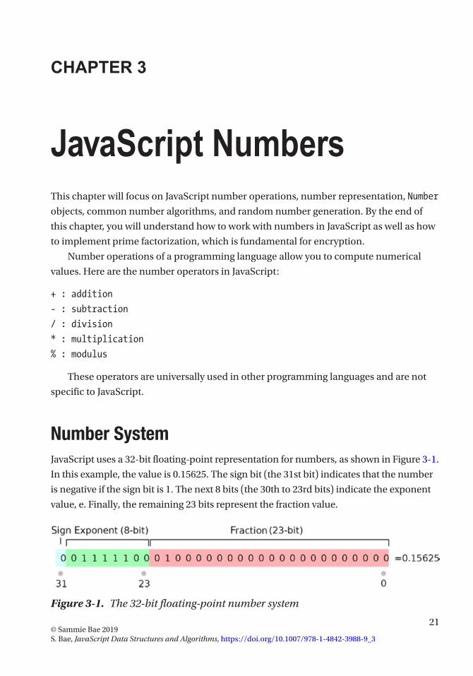
Number SystemJavaScript uses a 32-bit floating-point representation for numbers, as shown in Figure 3- 1.
In this example, the value is 0.15625. The sign bit (the 31st bit) indicates that the number
is negative if the sign bit is 1. The next 8 bits (the 30th to 23rd bits) indicate the exponent
value, e. Finally, the remaining 23 bits represent the fraction value.
Figure 3-1. The 32-bit floating-point number system

22
With the 32 bits, the value is computed by this esoteric formula:
value
sign e= -( ) ´ ´ +æ
èç
ö
ø÷
-
=-
-å1 2 1 2127
1
23
23t
ttb
Figure 3-1 shows the following break down of the 32 bits:
sign = 0
e = (0111100)2 = 124 (in base 10)
1 2 1 0 0 25 0
1
23
23+ = + + +=
--å
ii
ib .
This results in the following:
value = 1 x 2124-127 x 1.25 = 1 x 2-3 x 1.25 = 0.15625
With decimal fractions, this floating-point number system causes some rounding
errors in JavaScript. For example, 0.1 and 0.2 cannot be represented precisely.
Hence, 0.1 + 0.2 === 0.3 yields false.
1 0.1 + 0.2 === 0.3; // prints 'false'
To really understand why 0.1 cannot be represented properly as a 32-bit floating-
point number, you must understand binary. Representing many decimals in binary
requires an infinite number of digits. This because binary numbers are represented by 2n
where n is an integer.
While trying to calculate 0.1, long division will go on forever. As shown in Figure 3- 2,
1010 represents 10 in binary. Trying to calculate 0.1 (1/10) results in an indefinite
number of decimal points.
Chapter 3 JavaSCript NumberS

23
JavaScript Number ObjectLuckily, there are some built-in properties of the Number object in JavaScript that help
work around this.
Integer RoundingSince JavaScript uses floating point to represent all numbers, integer division does not work.
Integer division in programming languages like Java simply evaluates division
expressions to their quotient.
For example, 5/4 is 1 in Java because the quotient is 1 (although there is a remainder
of 1 left). However, in JavaScript, it is a floating point.
1 5/4; // 1.25
Figure 3-2. Long division for 0.1
Chapter 3 JavaSCript NumberS

24
This is because Java requires you to explicitly type the integer as an integer.
Hence, the result cannot be a floating point. However, if JavaScript developers want to
implement integer division, they can do one of the following:
Math.floor - rounds down to nearest integer
Math.round - rounds to nearest integer
Math.ceil - rounds up to nearest integer
Math.floor(0.9); // 0
Math.floor(1.1); // 1
Math.round(0.49); // 0
Math.round(0.5); // 1
Math.round(2.9); // 3
Math.ceil(0.1); // 1 Math.ceil(0.9); // 1 Math.ceil(21);
// 21 Math.ceil(21.01); // 22
Number.EPSILONNumber.EPSILON returns the smallest interval between two representable numbers.
This is useful for the problem with floating-point approximation.
1 function numberEquals(x, y) {
2 return Math.abs(x - y) < Number.EPSILON;
3 }
4
5 numberEquals(0.1 + 0.2, 0.3); // true
This function works by checking whether the difference between the two numbers
are smaller than Number.EPSILON. Remember that Number.EPSILON is the smallest
difference between two representable numbers. The difference between 0.1+0.2 and 0.3
will be smaller than Number.EPSILON.
MaximumsNumber.MAX_SAFE_INTEGER returns the largest integer.
1 Number.MAX_SAFE_INTEGER + 1 === Number.MAX_SAFE_INTEGER + 2; // true
Chapter 3 JavaSCript NumberS

25
This returns true because it cannot go any higher. However, it does not work for
floating-point decimals.
1 Number.MAX_SAFE_INTEGER + 1.111 === Number.MAX_SAFE_INTEGER + 2.022;
// false
Number.MAX_VALUE returns the largest floating-point number possible.
Number.MAX_VALUE is equal to 1.7976931348623157e+308.
1 Number.MAX_VALUE + 1 === Number.MAX_VALUE + 2; // true
Unlike like Number.MAX_SAFE_INTEGER, this uses double-precision floating-point
representation and works for floating points as well.
1 Number.MAX_VALUE + 1.111 === Number.MAX_VALUE + 2.022; // true
MinimumsNumber.MIN_SAFE_INTEGER returns the smallest integer.
Number.MIN_SAFE_INTEGER is equal to -9007199254740991.
1 Number.MIN_SAFE_INTEGER - 1 === Number.MIN_SAFE_INTEGER - 2; // true
This returns true because it cannot get any smaller. However, it does not work for
floating-point decimals.
1 Number.MIN_SAFE_INTEGER - 1.111 === Number.MIN_SAFE_INTEGER - 2.022;
// false
Number.MIN_VALUE returns the smallest floating-point number possible.
Number.MIN_VALUE is equal to 5e-324. This is not a negative number since it is the
smallest floating-point number possible and means that Number.MIN_VALUE is actually
bigger than Number.MIN_- SAFE_INTEGER.
Number.MIN_VALUE is also the closest floating point to zero.
1 Number.MIN_VALUE - 1 == -1; // true
This is because this is similar to writing 0 - 1 == -1.
Chapter 3 JavaSCript NumberS

26
Infinity
The only thing greater than Number.MAX_VALUE is Infinity, and the only thing smaller
than Number.MAX_SAFE_INTEGER is -Infinity.
1 Infinity > Number.MAX_SAFE_INTEGER; // true
2 -Infinity < Number.MAX_SAFE_INTEGER // true;
3 -Infinity -32323323 == -Infinity -1; // true
This evaluates to true because nothing can go smaller than -Infinity.
Size SummaryThis inequality summarizes the size of JavaScript numbers from smallest (left) to
largest (right):
-Infinity < Number.MIN_SAFE_INTEGER < Number.MIN_VALUE < 0 < Number.MAX_
SAFE_IN- TEGER < Number.MAX_VALUE < Infinity
Number AlgorithmsOne of the most discussed algorithms involving numbers is for testing whether a number
is a prime number. Let’s review this now.
Primality Test
A primality test can be done by iterating from 2 to n, checking whether modulus division
(remainder) is equal to zero.
1 function isPrime(n){
2 if (n <= 1) {
3 return false;
4 }
5
6 // check from 2 to n-1
7 for (var i=2; i<n; i++) {
8 if (n%i == 0) {
9 return false;
10 }
Chapter 3 JavaSCript NumberS

27
11 }
12
13 return true;
14 }
Time Complexity: O(n)
The time complexity is O(n) because this algorithm checks all numbers from 0 to n.
This is an example of an algorithm that can be easily improved. Think about how this
method iterates through 2 to n. Is it possible to find a pattern and make the algorithm
faster? First, any multiple of 2s can be ignored, but there is more optimization possible.
Let’s list some prime numbers.
2,3,5,7,11,13,17,19,23,29,31,37,41,43,47,53,59,61,67,71,73,79,83,89,97
This is difficult to notice, but all primes are of the form 6k ± 1, with the exception of
2 and 3 where k is some integer. Here’s an example:
5 = (6-1) , 7 = ((1*6) + 1), 13 = ((2*6) + 1) etc
Also realize that for testing the prime number n, the loop only has to test until the
square root of n. This is because if the square root of n is not a prime number, n is not a
prime number by mathematical definition.
1 function isPrime(n){
2 if (n <= 1) return false;
3 if (n <= 3) return true;
4
5 // This is checked so that we can skip
6 // middle five numbers in below loop
7 if (n%2 == 0 || n%3 == 0) return false;
8
9 for (var i=5; i*i<=n; i=i+6){
10 if (n%i == 0 || n%(i+2) == 0)
11 return false;
12 }
13
14 return true;
15 }
Chapter 3 JavaSCript NumberS
28
Time Complexity: O(sqrt(n))
This improved solution cuts the time complexity down significantly.
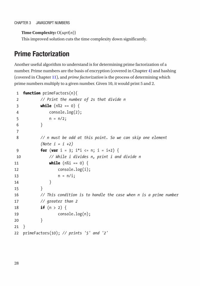
Prime FactorizationAnother useful algorithm to understand is for determining prime factorization of a
number. Prime numbers are the basis of encryption (covered in Chapter 4) and hashing
(covered in Chapter 11), and prime factorization is the process of determining which
prime numbers multiply to a given number. Given 10, it would print 5 and 2.
1 function primeFactors(n){
2 // Print the number of 2s that divide n
3 while (n%2 == 0) {
4 console.log(2);
5 n = n/2;
6 }
7
8 // n must be odd at this point. So we can skip one element
(Note i = i +2)
9 for (var i = 3; i*i <= n; i = i+2) {
10 // While i divides n, print i and divide n
11 while (n%i == 0) {
12 console.log(i);
13 n = n/i;
14 }
15 }
16 // This condition is to handle the case when n is a prime number
17 // greater than 2
18 if (n > 2) {
19 console.log(n);
20 }
21 }
22 primeFactors(10); // prints '5' and '2'
Chapter 3 JavaSCript NumberS

29
Time Complexity: O(sqrt(n))
This algorithm works by printing any number that is divisible by i without a
remainder. In the case that a prime number is passed into this function, it would be
handled by printing whether n is greater than 2.
Random Number GeneratorRandom number generation is important to simulate conditions. JavaScript has a built- in
function for generating numbers: Math.random().
Math.random() returns a float between 0 and 1.
You may wonder how you get random integers or numbers greater than 1.
To get floating points higher than 1, simply multiply Math.random() by the range.
Add or subtract from it to set the base.
Math.random() * 100; // floats between 0 and 100
Math.random() * 25 + 5; // floats between 5 and 30
Math.random() * 10 - 100; // floats between -100 and -90
To get random integers, simply use Math.floor(), Math.round(), or Math.ceil() to
round to an integer.
Math.floor(Math.random() * 100); // integer between 0 and 99
Math.round(Math.random() * 25) + 5; // integer between 5 and 30
Math.ceil(Math.random() * 10) - 100; // integer between -100 and -90
Exercises
1. Given three numbers x, y, and p, compute (xˆy) % p. (This is
modular exponentiation.)
Here, x is the base, y is exponent, and p is the modulus.
Modular exponentiation is a type of exponentiation performed
over a modulus, which is useful in computer science and used in
the field of public-key encryption algorithms.
At first, this problem seems simple. Calculating this is a one-line
solution, as shown here:
Chapter 3 JavaSCript NumberS

30
1 function modularExponentiation ( base, exponent, modulus ) {
2 return Math.pow(base,exponent) % modulus;
3 }
This does exactly what the question asks. However, it cannot
handle large exponents.
Remember that this is implemented with encryption algorithms.
In strong cryptography, the base is often at least 256 bit (78 digits).
Consider this case, for example:
Base: 6x1077, Exponent: 27, Modulus: 497
In this case, (6x1077)27 is a very large number and cannot be stored
in a 32-bit floating point.
There is another approach, which involves some math. One must
observe the following mathematical property:
For arbitrary a and b,
c % m = (a b) % m
c % m = [(a % m) (b % m)] % m
Using this mathematical property, you can iterate 1 to the
exponent, recalculating each time by multiplying the current
modulus value with the last.
Here is the pseudocode:
1 Set value = 1, current exponent = 0.
2 Increment current exponent by 1.
3 Set value = (base value) mod modulus until current
exponent is reached exponent
Example: Base: 4, Exponent: 3, Modulus: 5
4ˆ3 % 5 = 64 % 5 = 4
value = (lastValue x base ) % modulus:
value = (1 x 4) % 5 = 4 % 5 = 4
Chapter 3 JavaSCript NumberS

31
value = (4 x 4) % 5 = 16 % 5 = 1
value = (1 x 4) % 5 = 4 % 5 = 4
Finally, here is the code:
1 function modularExponentiation ( base, exponent, modulus ) {
2 if (modulus == 1) return 0;
3
4 var value = 1;
5
6 for ( var i=0; i<exponent; i++ ){
7 value = (value * base) % modulus;
8 }
9 return value;
10 }
Time Complexity: O(n)
The time complexity is O(n) where n is equal to the exponent value.
2. Print all primes less than n.
To do this, use the isPrime function covered in this chapter.
Simply iterate from 0 to n and print any prime numbers where
isPrime() evaluates to true.
1 function allPrimesLessThanN(n){
2 for (var i=0; i<n; i++) {
3 if (isPrime(i)){
4 console.log(i);
5 }
6 }
7 }
8
9 function isPrime(n){
10 if (n <= 1) return false;
11 if (n <= 3) return true;
12
Chapter 3 JavaSCript NumberS
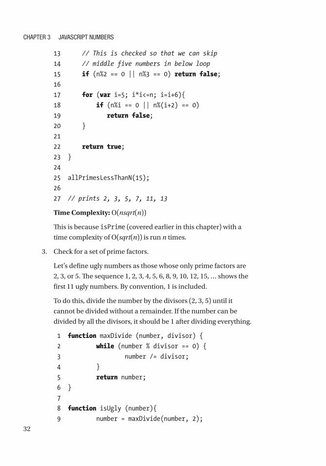
32
13 // This is checked so that we can skip
14 // middle five numbers in below loop
15 if (n%2 == 0 || n%3 == 0) return false;
16
17 for (var i=5; i*i<=n; i=i+6){
18 if (n%i == 0 || n%(i+2) == 0)
19 return false;
20 }
21
22 return true;
23 }
24
25 allPrimesLessThanN(15);
26
27 // prints 2, 3, 5, 7, 11, 13
Time Complexity: O(nsqrt(n))
This is because isPrime (covered earlier in this chapter) with a
time complexity of O(sqrt(n)) is run n times.
3. Check for a set of prime factors.
Let’s define ugly numbers as those whose only prime factors are
2, 3, or 5. The sequence 1, 2, 3, 4, 5, 6, 8, 9, 10, 12, 15, … shows the
first 11 ugly numbers. By convention, 1 is included.
To do this, divide the number by the divisors (2, 3, 5) until it
cannot be divided without a remainder. If the number can be
divided by all the divisors, it should be 1 after dividing everything.
1 function maxDivide (number, divisor) {
2 while (number % divisor == 0) {
3 number /= divisor;
4 }
5 return number;
6 }
7
8 function isUgly (number){
9 number = maxDivide(number, 2);
Chapter 3 JavaSCript NumberS

33
10 number = maxDivide(number, 3);
11 number = maxDivide(number, 5);
12 return number === 1;
13 }
Iterate this over n, and now the list of ugly numbers can be
returned.
1 function arrayNUglyNumbers (n) {
2 var counter = 0, currentNumber = 1,
uglyNumbers = [];
3
4 while ( counter != n ) {
5
6 if ( isUgly(currentNumber) ) {
7 counter++;
8 uglyNumbers.push(currentNumber);
9 }
10
11 currentNumber++;
12 }
13
14 return uglyNumbers;
15 }
Time Complexity for maxDivide(number, divisor):
O(logdivisor(number))
The time complexity of maxDivide is a logarithmic function which
depends on divisor and the number. When testing primes of 2,
3, and 5, the logarithmic of 2 (log2 (n)) yields the highest time
complexity.
Time Complexity for isUgly: O(log2(n))
Time Complexity for arrayNUglyNumbers: O(n(log2(n)))
The isUgly function is limited by the time complexity of maxDivide(number, 2).
Hence, arrayNUglyNumbers has n times that time complexity.
Chapter 3 JavaSCript NumberS

34
SummaryRecall that all numbers in JavaScript are in 32-bit floating point format. To get the
smallest possible floating point increment, you should use Number.EPILSON. The
maximum and minimum numbers of JavaScript can be summarized by the following
inequality:
-Infinity < Number.MIN_SAFE_INTEGER < Number.MIN_VALUE < 0
< Number.MAX_SAFE_INTEGER < Number.MAX_VALUE < Infinity
Prime number validation and prime factorization are concepts used in various
computer science applications such as encryption, as covered in Chapter 4. Finally,
random number generation in JavaScript works via Math.random().
Chapter 3 JavaSCript NumberS
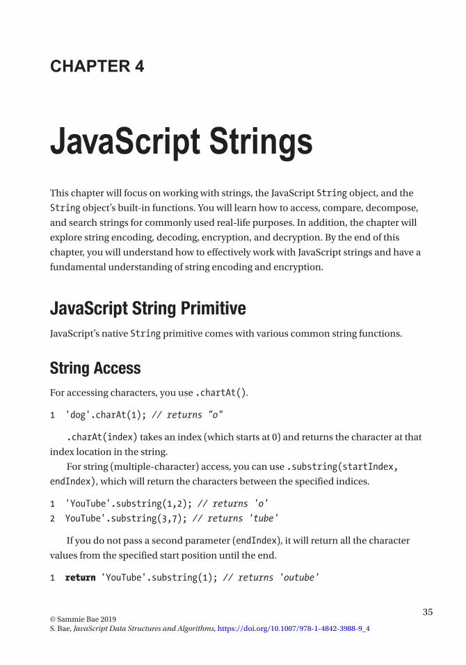
35© Sammie Bae 2019 S. Bae, JavaScript Data Structures and Algorithms, https://doi.org/10.1007/978-1-4842-3988-9_4
CHAPTER 4
JavaScript StringsThis chapter will focus on working with strings, the JavaScript String object, and the
String object’s built-in functions. You will learn how to access, compare, decompose,
and search strings for commonly used real-life purposes. In addition, the chapter will
explore string encoding, decoding, encryption, and decryption. By the end of this
chapter, you will understand how to effectively work with JavaScript strings and have a
fundamental understanding of string encoding and encryption.
JavaScript String PrimitiveJavaScript’s native String primitive comes with various common string functions.
String AccessFor accessing characters, you use .chartAt().
1 'dog'.charAt(1); // returns "o"
.charAt(index) takes an index (which starts at 0) and returns the character at that
index location in the string.
For string (multiple-character) access, you can use .substring(startIndex,
endIndex), which will return the characters between the specified indices.
1 'YouTube'.substring(1,2); // returns 'o'
2 YouTube'.substring(3,7); // returns 'tube'
If you do not pass a second parameter (endIndex), it will return all the character
values from the specified start position until the end.
1 return 'YouTube'.substring(1); // returns 'outube'

36
String ComparisonMost programming languages have a function that allows you to compare strings. In
JavaScript, this can be done simply by using less-than and greater-than operators.
1 var a = 'a';
2 var b = 'b';
3 console.log(a < b); // prints 'true'
This can be really useful for comparing strings when sorting algorithms, which is
covered later in the book.
However, if you are comparing two strings of different lengths, it starts comparing
from the start of the string until the length of the smaller string.
1 var a = 'add';
2 var b = 'b';
3
4 console.log(a < b); // prints 'true'
In this example, a and b are compared. Since a is smaller than b, a < b evaluates to
true.
1 var a = 'add';
2 var b = 'ab';
3 console.log(a < b); // prints 'false'
In this example, after 'a' and 'b' are compared, 'd' and 'b' are compared.
Processing cannot continue because everything in 'ab' has been looked at. This is the
same as comparing 'ad' with 'ab'.
1 console.log('add'<'ab' == 'ad'<'ab'); // prints 'true'
String SearchTo find a specific string within a string, you can use .indexOf(searchValue[,
fromIndex]). This takes a parameter that is the string to be searched as well as an
optional parameter for the starting index for the search. It returns the position of the
matching string, but if nothing is found, then -1 is returned. Note that this function is
case sensitive.
Chapter 4 JavaSCript StringS

37
1 'Red Dragon'.indexOf('Red'); // returns 0
2 'Red Dragon'.indexOf('RedScale'); // returns -1
3 'Red Dragon'.indexOf('Dragon', 0); // returns 4
4 'Red Dragon'.indexOf('Dragon', 4); // returns 4
5 'Red Dragon'.indexOf(", 9); // returns 9
To check for the occurrence of a search string inside a larger string, simply check
whether -1 was returned from .indexOf.
1 function existsInString (stringValue, search) {
2 return stringValue.indexOf(search) !== -1;
3 }
4 console.log(existsInString('red','r')); // prints 'true';
5 console.log(existsInString('red','b')); // prints 'false';
You can use an additional parameter to search after a certain index in a string.
An example is counting occurrences of certain letters . In the following example, the
occurrences of the character 'a' will be counted:
1 var str = "He's my king from this day until his last day";
2 var count = 0;
3 var pos = str.indexOf('a');
4 while (pos !== -1) {
5 count++;
6 pos = str.indexOf('a', pos + 1);
7 }
8 console.log(count); // prints '3'
Finally, startsWith returns true (boolean) if the string starts with the specified input,
and endsWith checks whether the string ends with the specified input.
1 'Red Dragon'.startsWith('Red'); // returns true
2 'Red Dragon'.endsWith('Dragon'); // returns true
3 'Red Dragon'.startsWith('Dragon'); // returns false
4 'Red Dragon'.endsWith('Red'); // returns false
Chapter 4 JavaSCript StringS

38
String DecompositionFor decomposing a string into parts, you can use .split(separator), which is a great
utility function. It takes one parameter (the separator) and creates an array of substrings.
1 var test1 = 'chicken,noodle,soup,broth';
2 test1.split(","); // ["chicken", "noodle", "soup", "broth"]
Passing an empty separator will create an array of all the characters.
1 var test1 = 'chicken';
2 test1.split(""); // ["c", "h", "i", "c", "k", "e", "n"]
This is useful for when there are items listed in a string. The string can be turned into
an array to easily iterate through them.
String Replace.replace(string, replaceString) replaces a specified string within a string variable
with another string.
1 "Wizard of Oz".replace("Wizard","Witch"); // "Witch of Oz"
Regular ExpressionsRegular expressions (regexes) are a set of characters that define a search pattern.
Learning how to use regexes is a massive task of its own, but as a JavaScript developer, it
is important you know the basics of regexes.
JavaScript also comes with the native object RegExp, which is used for regular
expressions.
The constructor for the RegExp object takes two parameters: the regular expression
and the optional match settings, as shown here:
i Perform case-insensitive matching
g Perform a global match (find all matches rather than stopping after
first match)
m Perform multiline matching
Chapter 4 JavaSCript StringS

39
RegExp has the following two functions:
• search(): Tests for matches in a string. This returns the index of the
match.
• match(): Tests for matches. This returns all the matches.
The JavaScript String object also has the following two regex-related functions that
accept the RegExp object as an argument:
• exec(): Tests for matches in a string. This returns the first match.
• test(): Tests for matches in a string. This returns true or false.
Basic RegexHere are the basic regex rules:
^: Indicates the start of a string/line
\d: Finds any digit
[abc]: Finds any character between the brackets
[^abc]: Finds any character not between the brackets
[0-9]: Finds any digit between the brackets
[^0-9]: Finds any digit not between the brackets
(x|y): Finds any of the alternatives specified
The following returns index 11, which is the index of the character D, which is the first
character of the matched regex:
1 var str = "JavaScript DataStructures";
2 var n = str.search(/DataStructures/);
3 console.log(n); // prints '11'
Commonly Used RegexesRegexes are immensely helpful for checking the validity of user input in JavaScript. One
common type of input check is to validate whether it has any numeric characters.
The following are five regexes that developers often use.
Chapter 4 JavaSCript StringS
40
Any Numeric Characters
/\d+/
1 var reg = /\d+/;
2 reg.test("123"); // true
3 reg.test("33asd"); // true
4 reg.test("5asdasd"); // true
5 reg.test("asdasd"); // false
Only Numeric Characters
/^\d+$/
1 var reg = /^\d+$/;
2 reg.test("123"); // true
3 reg.test("123a"); // false
4 reg.test("a"); // false
Floating Numeric Characters
/^[0-9]*.[0-9]*[1-9]+$/
1 var reg = /^[0-9]*.[0-9]*[1-9]+$/;
2 reg.test("12"); // false
3 reg.test("12.2"); // true
Only Alphanumeric Characters
/[a-zA-Z0-9] /
1 var reg = /[a-zA-Z0-9]/;
2 reg.test("somethingELSE"); // true
3 reg.test("hello"); // true
4 reg.test("112a"); // true
5 reg.test("112"); // true
6 reg.test("^"); // false
Chapter 4 JavaSCript StringS
41
Query String
/([^?=&]+)(=([^&]*))/
In web applications, web URLs often pass in parameters in the URL for routing or
database query purposes.
For example, for the URL http://your.domain/product.aspx?category=4&
product_id=2140&query=lcd+tv, the URL might respond to a back-end SQL query like
the following:
1 SELECT LCD, TV FROM database WHERE Category = 4 AND Product_id=2140;
To parse these parameters, regexes can be useful.
1 var uri = 'http://your.domain/product.aspx?category=4&product_id=2140&
query=lcd+tv' ;
2 var queryString = {};
3 uri.replace(
4 new RegExp ("([^?=&]+)(=([^&]*))?" , "g" ),
5 function ($0, $1, $2, $3) { queryString[$1] = $3; }
6 );
7 console.log('ID: ' + queryString['product_id' ]); // ID: 2140
8 console.log('Name: ' + queryString['product_name' ]); // Name: undefined
9 console.log('Category: ' + queryString['category' ]); // Category: 4
EncodingEncoding is a general concept in computer science that represents characters in a
specialized format for efficient transmission or storage.
All computer file types are encoded in specific structures.
For example, when you upload a PDF, the encoding may look like this:
1 JVBERi0xLjMKMSAwIG9iago8PCAvVHlwZSAvQ2F0YWxvZwovT3V0bGluZXMgMiAwIFIKL1Bh
Z2VzIDMgMCBS\
2 ID4+CmVuZG9iagoyIDAgb2JqCjw8IC9UeXBlIC9PdXRsaW5lcyAvQ291bnQgMCA+PgplbmR
vYmoKMyAwIG9i\
3 ago8PCAvVHlwZSAvUGFnZXMKL0tpZHMgWzYgMCBSCl0KL0NvdW50IDEKL1Jlc291cmNlcyA8
PAovUHJvY1Nl\
Chapter 4 JavaSCript StringS
42
4 dCA0IDAgUgovRm9udCA8PCAKL0YxIDggMCBSCj4+Cj4+Ci9NZWRpYUJveCBbMC4wMDAgMC4w
MDAgNjEyLjAw\
5 MCA3OTIuMDAwXQogPj4KZW5kb2JqCjQgMCBvYmoKWy9QREYgL1RleHQgXQplbmRvYmoKNSAw
IG9iago8PAov\
6 Q3JlYXRvciAoRE9NUERGKQovQ3JlYXRpb25EYXRlIChEOjIwMTUwNzIwMTMzMzIzKzAyJzAw
JykKL01vZERh\
7 dGUgKEQ6MjAxNTA3MjAxMzMzMjMrMDInMDAnKQo+PgplbmRvYmoKNiAwIG9iago8PCAvVHlw
ZSAvUGFnZQov\
8 UGFyZW50IDMgMCBSCi9Db250ZW50cyA3IDAgUgo+PgplbmRvYmoKNyAwIG9iago8PCAvRmls
dGVyIC9GbGF0\
9 ZURlY29kZQovTGVuZ3RoIDY2ID4+CnN0cmVhbQp4nOMy0DMwMFBAJovSuZxCFIxN9AwMzRTM
DS31DCxNFUJS\
10 FPTdDBWMgKIKIWkKCtEaIanFJZqxCiFeCq4hAO4PD0MKZW5kc3RyZWFtCmVuZG9iago4IDA
gb2JqCjw8IC9U\
11 eXBlIC9Gb250Ci9TdWJ0eXBlIC9UeXBlMQovTmFtZSAvRjEKL0Jhc2VGb250IC9UaW1lcy1
Cb2xkCi9FbmNv\
12 ZGluZyAvV2luQW5zaUVuY29kaW5nCj4+CmVuZG9iagp4cmVmCjAgOQowMDAwMDAwMDAwIDY
1NTM1IGYgCjAw\
13 MDAwMDAwMDggMDAwMDAgbiAKMDAwMDAwMDA3MyAwMDAwMCBuIAowMDAwMDAwMTE5IDAwMDA
wIG4gCjAwMDAw\
14 MDAyNzMgMDAwMDAgbiAKMDAwMDAwMDMwMiAwMDAwMCBuIAowMDAwMDAwNDE2IDAwMDAwIG4
gCjAwMDAwMDA0\
15 NzkgMDAwMDAgbiAKMDAwMDAwMDYxNiAwMDAwMCBuIAp0cmFpbGVyCjw8Ci9TaXplIDkKL1J
vb3QgMSAwIFIK\
16 L0luZm8gNSAwIFIKPj4Kc3RhcnR4cmVmCjcyNQolJUVPRgo=.....
This is a Base64-encoded PDF string. Data like this is often passed to the server when
a PDF file is uploaded.
Base64 EncodingThe btoa() function creates a Base64-encoded ASCII string from a string. Each character
in the string is treated as a byte (8 bits: eight 0 and 1s).
The .atob() function decodes a string of data that has been encoded using Base64
encoding. For example, the string “hello I love learning to computer program” in a
Base64-encoded string looks like this: aGVsbG8gSSBsb3ZlIGxlYXJuaW5nIHRvIGNvbXB
1dGVyIHByb2dyYW0.
Chapter 4 JavaSCript StringS

43
1 btoa('hello I love learning to computer program');
2 // aGVsbG8gSSBsb3ZlIGxlYXJuaW5nIHRvIGNvbXB1dGVyIHByb2dyYW0
1 atob('aGVsbG8gSSBsb3ZlIGxlYXJuaW5nIHRvIGNvbXB1dGVyIHByb2dyYW0');
2 // hello I love learning to computer program
Learn more about Base64 at https://en.wikipedia.org/wiki/Base64.
String ShorteningHave you ever wondered how URL-shortening sites such as Bit.ly work? A simplified URL
compression algorithm follows a certain structure, as shown here for www.google.com:
1. The database creates a unique integer-based ID for the URL.
In Figure 4-1, www.google.com has the entry 11231230 in the
database.
2. The integer ID is shortened into a string. When shortened with
Base62 encoding, 11231230 will be VhU2.
Relational Database
Id
O www.youtube.com
www.google.com
url
... ....
11231230
Figure 4-1. Database entries
Relational Database
Id url Shortened Id
awww.youtube.com
www.google.com VhU2
O
... .... ....
11231230
Figure 4-2. Database entries after shortening
Chapter 4 JavaSCript StringS

44
For the shortening part, the following algorithm can be used. There are 62 possible
letters and numbers, consisting of 26 lowercase letters, 26 uppercase letters, and 10
numbers (0 to 9).
1 var DICTIONARY = "abcdefghijklmnopqrstuvwxyzABCDEFGHIJKLMNOPQRSTUVWXYZ
0123456789" .split(");
2
3 function encodeId(num) {
4 var base = DICTIONARY.length;
5 var encoded = " ;
6
7 if (num === 0 ) {
8 return DICTIONARY[0 ];
9 }
10
11 while (num > 0 ) {
12 encoded += DICTIONARY[(num % base)];
13 num = Math .floor(num / base);
14 }
15
16 return reverseWord(encoded);
17 }
18
19 function reverseWord(str) {
20 var reversed = "" ;
21 for (var i = str.length - 1 ; i >= 0 ; i-- ) {
22 reversed += str.charAt(i);
23 }
24 return reversed;
25 }
26
27 function decodeId(id) {
28 var base = DICTIONARY.length;
29 var decoded = 0 ;
30
Chapter 4 JavaSCript StringS
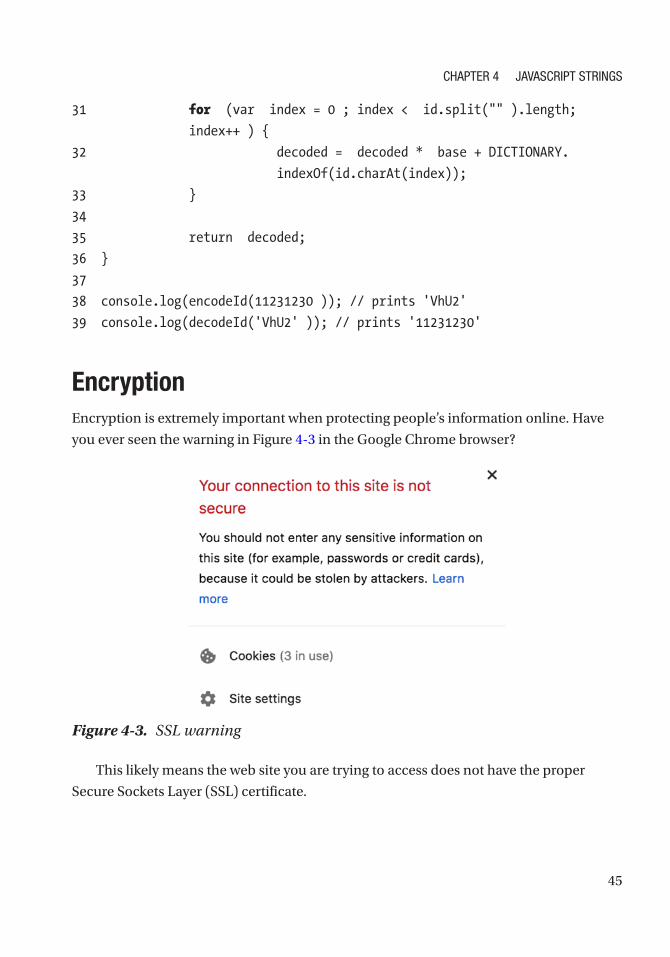
45
31 for (var index = 0 ; index < id.split("" ).length;
index++ ) {
32 decoded = decoded * base + DICTIONARY.
indexOf(id.charAt(index));
33 }
34
35 return decoded;
36 }
37
38 console.log(encodeId(11231230 )); // prints 'VhU2'
39 console.log(decodeId('VhU2' )); // prints '11231230'
EncryptionEncryption is extremely important when protecting people’s information online. Have
you ever seen the warning in Figure 4-3 in the Google Chrome browser?
This likely means the web site you are trying to access does not have the proper
Secure Sockets Layer (SSL) certificate.
Figure 4-3. SSL warning
Chapter 4 JavaSCript StringS

46
TSL is a standard security technology for establishing an encrypted link between
the server and the client (browser). The following are the simplified steps of the TSL
process. In this process, asymmetric encryption is used for different keys for encryption
and decryption by the server. The browser only uses symmetric encryption, which uses a
single key to both encrypt and decrypt the data.
1. The server sends its asymmetric public key to the browser.
2. The browser creates a symmetric key for the current session,
which is encrypted by the server’s asymmetric public key.
3. The server decrypts the browser’s session via its private key and
retrieves the session key.
4. Both systems have the session key and will use this to transmit
data securely.
This is secure because only the browser and the server know the session key. If the
browser was to connect to the same server the next day, a new session key would be created.
The SSL warning message is a sign that the browser and server may not be
encrypting the data on that connection.
The most commonly used public-key encryption algorithm is the RSA algorithm.
RSA EncryptionRSA is an encryption algorithm based on the difficulty of factoring large integers. In
RSA, two large prime numbers and a supplementary value are generated as the public
key. Anyone can use the public key to encrypt a message, but only those with the prime
factors can decode the message.
There are three phases in the process: key generation, encryption, and decryption.
Key generation: The public key (shared) and private key (kept
secret) are generated. The construction method of the keys
generated should be also secret.
1
32Browser Web Server
Figure 4-4. TSL process
Chapter 4 JavaSCript StringS

47
Encryption: The secret message can be encrypted via the public key.
Decryption: Only the private key can be used to decrypt the
message.
Here’s an overview of the algorithm:
1. Select two (usually large) prime numbers, p and q.
a. The product of p and q is denoted as n.
b. The product of (p-1) and (q-1) is denoted as phi.
2. Choose two exponents, e and d.
a. e is typically 3. Other values greater than 2 can be used.
b. d is a value such that (e × d) % phi = 1.
Encryption process is as shown:
m - message:
m^e % n = c
c - encrypted message
Decryption process is as shown:
c^d % n = m
This is the implementation of calculating d:
1 function modInverse(e, phi) {
2 var m0 = phi, t, q;
3 var x0 = 0, x1 = 1;
4
5 if (phi == 1)
6 return 0;
7
8 while (e > 1) {
9 // q is quotient
10 q = Math.floor(e / phi);
11
12 t = phi;
13
Chapter 4 JavaSCript StringS
48
14 // phi is remainder now, process same as
15 // Euclid's algo
16 phi = e % phi, e = t;
17
18 t = x0;
19
20 x0 = x1 - q * x0;
21
22 x1 = t;
23 }
24
25 // Make x1 positive
26 if (x1 < 0)
27 x1 += m0;
28
29 return x1;
30 }
31 modInverse(7,40); // 23
Key pairs of a public key and a private key also need to be generated.
1 function RSAKeyPair(p, q) {
2 // Need to check that they are primes
3 if (! (isPrime(p) && isPrime(q)))
4 return;
5
6 // Need to check that they're not the same
7 if (p==q)
8 return;
9
10 var n = p * q,
11 phi = (p-1)*(q-1),
12 e = 3,
13 d = modInverse(e,phi);
14
Chapter 4 JavaSCript StringS

49
15 // Public key: [e,n], Private key: [d,n]
16 return [[e,n], [d,n]]
17 }
Let’s pick 5 and 11 as the primes and see an example where message is 50.
1 RSAKeyPair(5,11); //Public key: [3,55], Private key: [27,55]
p = 5, 11
n = p x q = 55
phi = (5-1) x (11-1) = 4 x 10 = 40
e = 3
(e x d) % phi = 1 (3 x d) % 40 = 1
(81) % 40 = 1. 81 = 3 x d = 3 x 27
d = 27
Encryption:
m - message: 50
m^e % n = c
50^3 % 55 = 40
Encrypted message.,c:
40
Decryption:
c^d % n = m
40^27 % 55 = 50
This fully encrypts 50, and the receiver can decrypt that back to 50. Typically the
prime numbers chosen are very large for the RSA algorithm. This is because the prime
factorization of large numbers takes a long time to compute. Today’s standard is to
use a 4,096-bit prime product. Computing its prime factors would take years even for
advanced computers to compute. Figure 4-5 shows the largest possible value for a
4,096-bit number.
Chapter 4 JavaSCript StringS

50
SummaryVarious natively implemented string functions were covered in this chapter and are
summarized in Table 4-1.
Figure 4-5. 24096
Chapter 4 JavaSCript StringS

51
In addition, a JavaScript native Regex object can be used for commonly used string
validation. Table 4-2 provides a summary.
Table 4-1. String Function Summary
Function Usage
charAt(index) accesses a single character at index
substring(startIndex,
endIndex)
accesses part of string from startIndex to endIndex
str1 > str2 returns true if str1 is lexicographically bigger than str2
indexOf(str, startIndex) index of the desired str starting at startIndex
str.split(delimiter) Breaks a string into an array with the specified delimiter
str.replace(original,new) replaces original with new
Table 4-2. Regex Summary
Regex Pattern Usage
/\d+/ any numeric characters
/^\d+$/ Only numeric characters
/^[0-9]*.[0-9]*[1-9]+$/ Float numeric characters
/[a-zA-Z0-9] / Only alphanumeric characters
Chapter 4 JavaSCript StringS

53© Sammie Bae 2019 S. Bae, JavaScript Data Structures and Algorithms, https://doi.org/10.1007/978-1-4842-3988-9_5
CHAPTER 5
JavaScript ArraysThis chapter will focus on working with JavaScript arrays. As a JavaScript developer, you
will use the array often; it is the most commonly used data structure. Arrays in JavaScript
come with a lot of built-in methods. In fact, there are various ways to do the same type of
array operations for each use case. By the end of this chapter, you will understand how to
work with arrays and be able to choose the right method for the situation.
Introducing ArraysArrays are one of the most fundamental data structures. If you have ever programmed
before, you’ve most likely used an array.
1 var array1 = [1,2,3,4];
For any data structure, developers are interested in time and space complexity
associated with the four fundamental operations: access, insertion, deletion, and search.
(For a review of Big-O notations, please refer to Chapter 1.)
InsertionInsertion means adding a new element inside a data structure. JavaScript implements
array insertion with the .push(element) method. This method adds a new element at
the end of the array.
1 var array1 = [1,2,3,4];
2 array1.push(5); //array1 = [1,2,3,4,5]
3 array1.push(7); //array1 = [1,2,3,4,5,7]
4 array1.push(2); //array1 = [1,2,3,4,5,7,2]

54
The time complexity of this operation is O(1) in theory. It should be noted that,
practically, this depends on the JavaScript engine that runs the code. This applies to all
natively supported JavaScript objects.
DeletionJavaScript implements array deletion with the .pop() method. This method removes the
last-added element of the array. This also returns the removed element.
1 var array1 = [1,2,3,4];
2 array1.pop(); //returns 4, array1 = [1,2,3]
3 array1.pop(); //returns 3, array1 = [1,2]
The time complexity of .pop is O(1) similarly to .push.
Another way to remove an element from an array is with the .shift() method. This
method will remove the first element and return it.
1 array1 = [1,2,3,4];
2 array1.shift(); //returns 1, array1 = [2,3,4]
3 array1.shift(); //returns 2, array1 = [3,4]
AccessAccessing an array at a specified index only takes O(1) because this process uses that
index to get the value directly from the address in memory. It is done by specifying the
index (remember that indexing starts at 0).
1 var array1 = [1,2,3,4];
2 array1[0]; //returns 1
3 array1[1]; //returns 2
IterationIteration is the process of accessing each of the items contained within a data structure.
There are multiple ways to iterate through an array in JavaScript. They all have a time
complexity of O(n) since the iteration is visiting n number of elements.
Chapter 5 JavaSCript arrayS

55
for (Variables; Condition; Modification)for is the most common method of iteration. It is most often used in this form:
1 for ( var i=0, len=array1.length; i<len; i++ ) {
2 console.log(array1[i]);
3 }
The previous code simply means initialize the variable i, check whether the
condition is false before executing the body (i<len), and then modify (i++) until the
condition is false. Similarly, you can use a while loop. However, the counter will have to
be set outside.
1 var counter=0;
2 while(counter<array1.length){
3 // insert code here
4 counter++;
5 }
You can implement an infinite loop using a while loop, as shown here:
1 while(true){
2 if (breakCondition) {
3 break;
4 }
5 }
Similarly, a for loop can implement an infinite loop by not setting a condition, as
shown here:
1 for ( ; ;) {
2 if (breakCondition) {
3 break
4 }
5 }
Chapter 5 JavaSCript arrayS

56
for ( in )Another way to iterate a JavaScript array is to call the indices one by one. The variable
specified before in is the index of the array, as follows:
1 var array1 = ['all','cows','are','big'];
2
3 for (var index in array1) {
4 console.log(index);
5 }
This prints the following: 0,1,2,3.
To print the content, use this:
1 for (var index in array1) {
2 console.log(array1[index]);
3 }
This prints all, cows, are, and big.
for ( of )The variable specified before of is the element (the value) of the array, as follows:
1 for (var element of array1) {
2 console.log(element);
3 }
This prints out all, cows, are, and big.
forEach( )The big difference between forEach and other methods of iteration is that forEach
cannot break out of the iteration or skip certain elements in the array. forEach is more
expressive and explicit by going through each element.
Chapter 5 JavaSCript arrayS

57
1 var array1 = ['all','cows','are','big'];
2
3 array1.forEach( function (element, index){
4 console.log(element);
5 });
6
7 array1.forEach( function (element, index){
8 console.log(array1[index]);
9 });
Both print all, cows, are, and big.
Helper FunctionsThe following sections discuss other commonly used helper functions for processing.
In addition, working with arrays will be covered.
.slice(begin,end)This helper function returns a portion of an existing array without modifying the array.
.slice() takes two parameters: the beginning index and the ending index of the array.
1 var array1 = [1,2,3,4];
2 array1.slice(1,2); //returns [2], array1 = [1,2,3,4]
3 array1.slice(2,4); //returns [3,4], array1 = [1,2,3,4]
If only the beginning index is passed, the ending will be assumed to be the maximum
index.
1 array1.slice(1); //returns [2,3,4], array1 = [1,2,3,4]
2 array1.slice(1,4); //returns [2,3,4], array1 = [1,2,3,4]
If nothing is passed, this function simply returns a copy of the array. It should be
noted that array1.slice() === array1 evaluates to false. This is because although the
contents of the arrays are the same, the memory addresses at which those arrays reside
are different.
1 array1.slice(); //returns [1,2,3,4], array1 = [1,2,3,4]
Chapter 5 JavaSCript arrayS

58
This is useful for copying an array in JavaScript. Remember that arrays in JavaScript
are reference-based, meaning that if you assign a new variable to an array, changes to
that variable apply to the original array.
1 var array1 = [1,2,3,4],
2 array2 = array1;
3
4 array1 // [1,2,3,4]
5 array2 // [1,2,3,4]
6
7 array2[0] = 5;
8
9 array1 // [5,2,3,4]
10 array2 // [5,2,3,4]
The changing element of array2 changed the original array by accident because it is
a reference to the original array. To create a new array, you can use .from().
1 var array1 = [1,2,3,4];
2 var array2 = Array.from(array1);
3
4 array1 // [1,2,3,4]
5 array2 // [1,2,3,4]
6
7 array2[0] = 5;
8
9 array1 // [1,2,3,4]
10 array2 // [5,2,3,4]
.from() takes O(n), where n is the size of the array. This is intuitive because copying
the array requires copying all n elements of the array.
.splice(begin,size,element1,element2…)This helper function returns and changes the contents of an array by removing existing
elements and/or adding new elements.
Chapter 5 JavaSCript arrayS

59
.splice() takes three parameters: the beginning index, the size of things to be
removed, and the new elements to add. New elements are added at the position
specified by the first parameter. It returns the removed elements.
1 var array1 = [1,2,3,4];
2 array1.splice(); //returns [], array1 = [1,2,3,4]
3 array1.splice(1,2); //returns [2,3], array1 = [1,4]
This example demonstrates removal. [2,3] was returned because it selected two
items starting from an index of 1.
1 var array1 = [1,2,3,4];
2 array1.splice(); //returns [], array1 = [1,2,3,4]
3 array1.splice(1,2,5,6,7); //returns [2,3],array1 = [1,5,6,7,4]
Anything (any object type) can be added to the array. This is the beauty (and odd
part) of JavaScript.
1 var array1 = [1,2,3,4];
2 array1.splice(1,2,[5,6,7]); //returns [2,3], array1 = [1,[5,6,7],4]
3 array1 = [1,2,3,4];
4 array1.splice(1,2,{'ss':1}); //returns [2,3], array1 = [1,{'ss':1},4]
.splice() is, worst case, O(n). Similarly to copying, if the range specified is the
whole array, each n item has to be removed.
.concat()This adds new elements to the array at the end of the array and returns the array.
1 var array1 = [1,2,3,4];
2 array1.concat(); //returns [1,2,3,4], array1 = [1,2,3,4]
3 array1.concat([2,3,4]); //returns [1,2,3,4,2,3,4],array1 = [1,2,3,4]
.length PropertyThe .length property returns the size of the array. Changing this property to a lower size
can delete elements from the array.
Chapter 5 JavaSCript arrayS
60
1 var array1 = [1,2,3,4];
2 console.log(array1.length); //prints 4
3 array1.length = 3; // array1 = [1,2,3]
Spread OperatorThe spread operator, denoted by three periods (...), is used to expand arguments where
zero arguments are expected.
1 function addFourNums(a, b, c, d) {
2 return a + b + c + d;
3 }
4 var numbers = [1, 2, 3, 4];
5 console.log(addFourNums(...numbers)); // 10
Both the Math.max and Math.min functions take an unlimited number of parameters,
so you can use the spread operator for the following operations.
To find the maximum in an array, use this:
1 var array1 = [1,2,3,4,5];
2 Math.max(array1); // 5
To find the minimum in an array, use this:
1 var array2 = [3,2,-123,2132,12];
2 Math.min(array2); // -123
ExercisesAll the code for the exercises can be found on GitHub.1
FIND TWO ARRAY ELEMENTS IN AN ARRAY THAT ADD UP TO A NUMBER
problem: Given the array arr, find and return two indices of the array that add up to weight
or return -1 if there is no combination that adds up to weight.
1 https://github.com/Apress/js-data-structures-and-algorithms
Chapter 5 JavaSCript arrayS

61
For example, in an array like [1,2,3,4,5], what numbers add up to 9?
the answers are 4 and 5, of course.
the simple solution is to try every combination by having two for loops, as shown here:
1 function findSum(arr, weight) {
2 for (var i=0,arrLength=arr.length; i<arrLength; i++){
3 for (var j=i+1; j<arrLength; j++) {
4 if (arr[i]+arr[j]==weight){
5 return [i,j];
6 }
7 }
8 }
9 return -1;
10 }
this solution iterates through an array looking to see whether a matching pair exists.
two for loops over n elements of the array yields a high time complexity. however, no extra
memory was created. Similar to how time complexity describes the time required relative to
input size, n, to finish the algorithm, the space complexity describes the additional memory
needed for implementation. the space complexity, O(1), is constant.
Time Complexity: O(n2)
Space Complexity: O(1)
Let’s think about how to do this in linear time of O(n).
What if any previously seen array elements were stored and could be checked easily?
here’s the input:
1 var arr = [1,2,3,4,5];
2 var weight = 9;
here, 4 and 5 are the combination, and their indices are [3,4]. how could it be determined
that a solution exists when 5 is visited?
if the current value is at 5 and the weight is 9, the remaining required weight is just 4 (9-5=4).
Since 4 is shown before 5 in the array, this solution can work in O(n). Finally, to store the seen
elements, use a JavaScript object as a hash table. the implementation and use of a hash table
will be discussed in later chapters. Storing into and retrieving a JavaScript object property is
O(1) in time.
Chapter 5 JavaSCript arrayS

62
1 function findSumBetter(arr, weight) {
2 var hashtable = {};
3
4 for (var i=0, arrLength=arr.length; i<arrLength; i++) {
5 var currentElement = arr[i],
6 difference = weight - currentElement;
7
8 // check the right one already exists
9 if (hashtable[currentElement] != undefined) {
10 return [i, hashtable[weight-currentElement]];
11 } else {
12 // store index
13 hashtable[difference] = i;
14 }
15 }
16 return -1;
17 }
Time Complexity: O(n)
Space Complexity: O(n)
Storing into a hash table and looking an item up from a hash table is only O(1). Space
complexity has increased to O(n) to store the visited array indices inside the hash table.
IMPLEMENT THE ARRAY.SLICE() FUNCTION FROM SCRATCH
Let’s review what the .slice() function does.
.slice() takes two parameters: the beginning index and the last ending index of the array.
it returns a portion of an existing array without modifying the array function arraySlice
(array, beginIndex, endIndex).
1 function arraySlice(array, beginIndex, endIndex) {
2 // If no parameters passed, return the array
3 if (! beginIndex && ! endIndex) {
4 return array;
5 }
6
Chapter 5 JavaSCript arrayS

63
7 // If only beginning index is found, set endIndex to size
8 endIndex = array.length;
9
10 var partArray = [];
11
12 // If both begin and end index specified return the part of the array
13 for (var i = beginIndex; i < endIndex; i++ ) {
14 partArray.push(array[i]);
15 }
16
17 return partArray;
18 }
19 arraySlice([1 , 2 , 3 , 4 ], 1 , 2 ); // [2]
20 arraySlice([1 , 2 , 3 , 4 ], 2 , 4 ); // [3,4]
Time Complexity: O(n)
Space Complexity: O(n)
the time complexity is O(n) because all n items in the array must be accessed. Space
complexity is also O(n) to hold all n items when copying the array.
FIND THE MEDIAN OF TWO SORTED ARRAYS OF THE SAME SIZE
recall that median in an even number of a set is the average of the two middle numbers.
if the array is sorted, this is simple.
here’s an example:
[1,2,3,4] has the median of (2+3)/2 = 2.5.
1 function medianOfArray(array) {
2 var length = array.length;
3 // Odd
4 if (length % 2 == 1) {
5 return array[Math.floor(length/2)];
6 } else {
7 // Even
8 return (array[length/2]+array[length/2 - 1])/2;
Chapter 5 JavaSCript arrayS

64
9 }
10 }
Now, you can iterate through both of the arrays and compare which is bigger to track the
median. if the two arrays are the same size, the total size will be an even number.
this is because both two even numbers and two odd numbers add up to an even number.
please refer to Chapter 8 for more background.
Since both of the arrays are sorted, this function can be recursively called. each time, it checks
which median is greater.
if the second array’s median is greater, the first array is cut in half, and only the higher half is
passed recursively.
if the first array’s median is greater, the second array is cut in half, and only the higher half
is passed in as the first array for the next function call because the array2 parameter in
the function must always be bigger than the array1 parameter. Finally, the size of the array
represented as pos is required to check whether the size of the array is even or odd.
here’s another example:
array1 = [1,2,3] and array2 = [4, 5, 6]
here, the median of array1 is 2, and the median of array2 is 5. So, the median must be
present within [2,3] and [4,5]. Since there are only four elements left, the median can be
computed as follows:
max(arr1[0], arr2[0]) + min(arr1[1], arr2[1]) / 2;
1 function medianOfArray(array) {
2 var length = array.length;
3 // Odd
4 if (length % 2 == 1 ) {
5 return array[Math .floor(length / 2 )];
6 } else {
7 // Even
8 return (array[length / 2 ] + array[length / 2 - 1 ]) / 2 ;
9 }
10 }
11 // arr2 is the bigger array
12 function medianOfTwoSortedArray(arr1, arr2, pos) {
Chapter 5 JavaSCript arrayS
65
13 if (pos <= 0 ) {
14 return -1 ;
15 }
16 if (pos == 1 ) {
17 return (arr1[0] + arr2[0]) / 2 ;
18 }
19 if (pos == 2 ) {
20 return (Math .max(arr1[0], arr2[0]) + Math .min(arr1[1],
arr2[1])) / 2 ;
21 }
22
23 var median1 = medianOfArray(arr1),
24 median2 = medianOfArray(arr2);
25
26 if (median1 == median2) {
27 return median1;
28 }
29
30 var evenOffset = pos % 2 == 0 ? 1 : 0 ,
31 offsetMinus = Math .floor(pos / 2 ) - evenOffset,
32 offsetPlus = Math .floor(pos / 2 ) + evenOffset;
33
34
35 if (median1 < median2) {
36 return medianOfTwoSortedArray(arr1.slice(offsetMinus), arr2.
slice(offsetMinus), offsetPlus);
37 } else {
38 return medianOfTwoSortedArray(arr2.slice(offsetMinus), arr1.
slice(offsetMinus), offsetPlus);
39 }
40 }
41
42 medianOfTwoSortedArray([1 , 2 , 3 ], [4 , 5 , 6 ], 3 ); // 3.5
43 medianOfTwoSortedArray([11 , 23 , 24 ], [32 , 33 , 450 ], 3 ); // 28
44 medianOfTwoSortedArray([1 , 2 , 3 ], [2 , 3 , 5 ], 3 ); // 2.5
Time Complexity: O(log2(n))
By cutting the array size by half each time, logarithmic time complexity is achieved.
Chapter 5 JavaSCript arrayS

66
FIND COMMON ELEMENTS IN K-SORTED ARRAYS
1 var arr1 = [1, 5, 5, 10];
2 var arr2 = [3, 4, 5, 5, 10];
3 var arr3 = [5, 5, 10, 20];
4 var output = [5 ,10];
in this example with three arrays, k=3.
to do this, simply iterate over each array and count instances of every element. however, do not
track repeated ones (5 and 5.5 should be counted once in one array iteration). to do this, check
whether the last element is the same before incrementing. this will work only if it is sorted.
after all three arrays have been iterated, iterate through the hash table’s properties. if the
value matches 3, it means that the number showed up in all three arrays. this can be
generalized to k number of arrays by putting the k-loop check into another for loop.
1 function commonElements(kArray) {
2 var hashmap = {},
3 last, answer = [];
4
5 for (var i = 0 , kArrayLength = kArray.length; i < kArrayLength;
i++ ) {
6 var currentArray = kArray[i];
7 last = null ;
8 for (var j = 0 , currentArrayLen = currentArray.length;
9 j < currentArrayLen; j++ ) {
10 var currentElement = currentArray[j];
11 if (last != currentElement) {
12 if (! hashmap[currentElement]) {
13 hashmap[currentElement] = 1 ;
14 } else {
15 hashmap[currentElement]++ ;
16 }
17 }
18 last = currentElement;
19 }
20 }
21
Chapter 5 JavaSCript arrayS

67
22 // Iterate through hashmap
23 for (var prop in hashmap) {
24 if (hashmap[prop] == kArray.length) {
25 answer.push(parseInt (prop));
26 }
27 }
28 return answer;
29 }
30
31 commonElements([[1 ,2 ,3 ],[1 ,2 ,3 ,4 ],[1 ,2 ]]); // [ 1, 2 ]
Time Complexity: O(kn)
Space Complexity: O(n)
here, n is longest array length, and k is the number of arrays.
JavaScript Functional Array MethodsSome parts of JavaScript can be written just like a functional programming language.
Unlike imperative programming, JavaScript does not focus on the state of the program.
It does not use loops, only function (method) calls. You can learn more about functional
programming in JavaScript from Beginning Functional JavaScript by Anto Aravinth
(Apress, 2017).
In this section, only three functional array methods in JavaScript will be explored:
map, filter, and reduce. These methods do not change the original array contents.
MapThe map function applies passed function transformation to every element in the array
and returns a new array with those transformations applied.
For example, you can multiply every element by 10, as shown here:
1 [1,2,3,4,5,6,7].map(function (value){
2 return value*10;
3 });
4 // [10, 20, 30, 40, 50, 60, 70]
Chapter 5 JavaSCript arrayS

68
FilterThe filter function returns only those elements of the array that meet a passed
condition parameter. Again, this does not change the original array.
For example, this filters elements greater than 100:
1 [100,2003,10,203,333,12].filter(function (value){
2 return value > 100;
3 });
4 // [2003, 203, 333]
ReduceThe reduce function combines all the elements in the array into one value using a
passed transformation function parameter.
For example, this adds all the elements:
1 var sum = [0,1,2,3,4].reduce( function (prevVal, currentVal, index,
array) {
2 return prevVal + currentVal;
3 });
4 console.log(sum); // prints 10
This function also can take initialValue as its second argument, which initializes
the reduce value. For example, providing an initialValue of 1 in the previous example
will yield 11, as shown here:
1 var sum = [0,1,2,3,4].reduce( function (prevVal, currentVal, index,
array) {
2 return prevVal + currentVal;
3 }, 1);
4 console.log(sum); // prints 11
Multidimensional ArraysUnlike Java and C++, JavaScript does not have multidimensional arrays (see Figure 5-1).
Chapter 5 JavaSCript arrayS

69
Instead, there are “jagged” arrays. A jagged array is an array whose elements are
arrays. The elements of a jagged array can be of different dimensions and sizes (see
Figure 5-2).
Here is a helper function to create a jagged array like the one in Figure 5-3:
1 function Matrix(rows, columns) {
2 var jaggedarray = new Array(rows);
3 for (var i=0; i < columns; i +=1) {
4 jaggedarray[i]=new Array(rows);
5 }
6 return jaggedarray;
7 }
8 console.log(Matrix(3,3));
Figure 5-1. Multidimensional array
Figure 5-2. Jagged array
Chapter 5 JavaSCript arrayS

70
To access elements in a jagged array, specify a row and a column (see Figure 5-4).
1 var matrix3by3 = [[1,2,3],[4,5,6],[7,8,9]];
2 matrix3by3[0]; // [1,2,3]
3 matrix3by3[1]; // [4,5,6]
4 matrix3by3[1]; // [7,8,9]
5
6 matrix3by3[0][0]; // 1
7 matrix3by3[0][1]; // 2
8 matrix3by3[0][2]; // 3
9
10 matrix3by3[1][0]; // 4
11 matrix3by3[1][1]; // 5
Figure 5-3. Three-by-three matrix
Figure 5-4. Three-by-three matrix of numbers
Chapter 5 JavaSCript arrayS
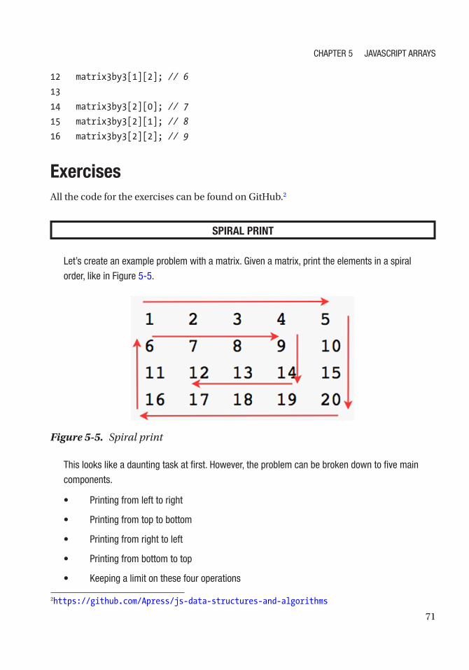
71
12 matrix3by3[1][2]; // 6
13
14 matrix3by3[2][0]; // 7
15 matrix3by3[2][1]; // 8
16 matrix3by3[2][2]; // 9
ExercisesAll the code for the exercises can be found on GitHub.2
SPIRAL PRINT
Let’s create an example problem with a matrix. Given a matrix, print the elements in a spiral
order, like in Figure 5-5.
this looks like a daunting task at first. however, the problem can be broken down to five main
components.
• printing from left to right
• printing from top to bottom
• printing from right to left
• printing from bottom to top
• Keeping a limit on these four operations
Figure 5-5. Spiral print
2 https://github.com/Apress/js-data-structures-and-algorithms
Chapter 5 JavaSCript arrayS

72
in other words, keep four key variables that indicate the following:
• top row
• Bottom row
• Left column
• right column
each time one of the four print functions is successfully executed, simply increment one of
the four variables. For example, after printing the top row, increment it by 1.
1 var M = [
2 [1, 2, 3, 4, 5],
3 [6, 7, 8, 9, 10],
4 [11, 12, 13, 14, 15],
5 [16, 17, 18, 19, 20]
6 ];
7 function spiralPrint(M) {
8 var topRow = 0,
9 leftCol = 0,
10 btmRow = M.length - 1,
11 rightCol = M[0].length - 1;
12
13 while (topRow < btmRow && leftCol < rightCol) {
14 for (var col = 0; col <= rightCol; col++) {
15 console.log(M[topRow][col]);
16 }
17 topRow++;
18 for (var row = topRow; row <= btmRow; row++) {
19 console.log(M[row][rightCol]);
20 }
21 rightCol--;
22 if (topRow <= btmRow) {
23 for (var col = rightCol; col >= 0; col--) {
24 console.log(M[btmRow][col]);
25 }
26 btmRow--;
27 }
28 if (leftCol <= rightCol) {
Chapter 5 JavaSCript arrayS
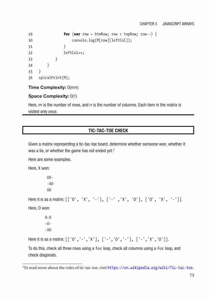
73
29 for (var row = btmRow; row > topRow; row--) {
30 console.log(M[row][leftCol]);
31 }
32 leftCol++;
33 }
34 }
35 }
36 spiralPrint(M);
Time Complexity: O(mn)
Space Complexity: O(1)
here, m is the number of rows, and n is the number of columns. each item in the matrix is
visited only once.
TIC-TAC-TOE CHECK
Given a matrix representing a tic-tac-toe board, determine whether someone won, whether it
was a tie, or whether the game has not ended yet.3
here are some examples.
here, X won:
OX-
-XO
OX
here it is as a matrix: [['O', 'X', '-'], ['-' ,'X', 'O'], ['O', 'X', '-']].
here, O won:
O-X
-O-
-XO
here it is as a matrix: [['O','-','X'], ['-','O','-'], ['-','X','O']].
to do this, check all three rows using a for loop, check all columns using a for loop, and
check diagonals.
3 To read more about the rules of tic-tac-toe, visit https://en.wikipedia.org/wiki/Tic-tac-toe.
Chapter 5 JavaSCript arrayS

74
1 function checkRow ( rowArr, letter ) {
2 for ( var i=0; i < 3; i++) {
3 if (rowArr[i]!=letter) {
4 return false;
5 }
6 }
7 return true;
8 }
9
10 function checkColumn ( gameBoardMatrix, columnIndex, letter ) {
11 for ( var i=0; i < 3; i++) {
12 if (gameBoardMatrix[i][columnIndex]!=letter) {
13 return false;
14 }
15 }
16 return true;
17 }
18
19 function ticTacToeWinner ( gameBoardMatrix, letter) {
20
21 // Check rows
22 var rowWin = checkRow(gameBoardMatrix[0], letter)
23 || checkRow(gameBoardMatrix[1], letter)
24 || checkRow(gameBoardMatrix[2], letter);
25
26 var colWin = checkColumn(gameBoardMatrix, 0, letter)
27 || checkColumn(gameBoardMatrix, 1, letter)
28 || checkColumn(gameBoardMatrix, 2, letter);
29
30 var diagonalWinLeftToRight = (gameBoardMatrix[0][0]==letter &&
gameBoardMatrix[1][1]==letter && gameBoardMatrix[2][2]==letter);
31 var diagonalWinRightToLeft = (gameBoardMatrix[0][2]==letter &&
gameBoardMatr ix[1][1]==letter && gameBoardMatrix[2][0]==letter);
32
33 return rowWin || colWin || diagonalWinLeftToRight ||
diagonalWinRightToLeft;
34 }
35
Chapter 5 JavaSCript arrayS
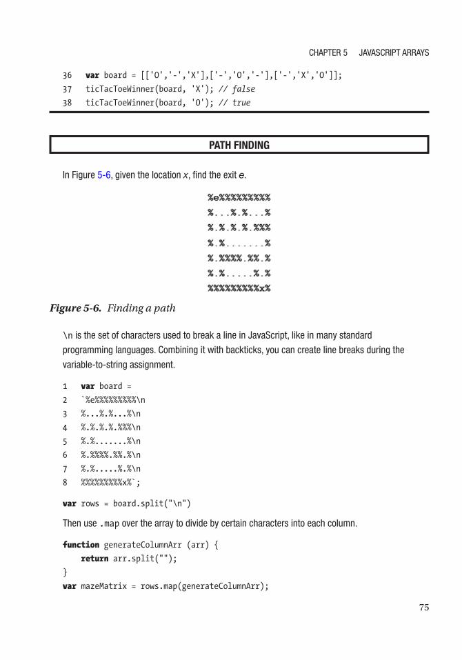
75
36 var board = [['O','-','X'],['-','O','-'],['-','X','O']];
37 ticTacToeWinner(board, 'X'); // false
38 ticTacToeWinner(board, 'O'); // true
PATH FINDING
in Figure 5-6, given the location x, find the exit e.
\n is the set of characters used to break a line in JavaScript, like in many standard
programming languages. Combining it with backticks, you can create line breaks during the
variable-to-string assignment.
1 var board =
2 `%e%%%%%%%%%\n
3 %...%.%...%\n
4 %.%.%.%.%%%\n
5 %.%.......%\n
6 %.%%%%.%%.%\n
7 %.%.....%.%\n
8 %%%%%%%%%x%`;
var rows = board.split("\n")
then use .map over the array to divide by certain characters into each column.
function generateColumnArr (arr) {
return arr.split("");
}
var mazeMatrix = rows.map(generateColumnArr);
Figure 5-6. Finding a path
Chapter 5 JavaSCript arrayS

76
this will generate the proper matrix where each row is an array of the characters and the
board is the array of those rows.
Now, first find the entrance, e, and exit, x. this function will return the row position, i, and the
column position, j, of the character to be searched for:
1 function findChar(char , mazeMatrix) {
2 var row = mazeMatrix.length,
3 column = mazeMatrix[0 ].length;
4
5 for (var i = 0 ; i < row; i++ ) {
6 for (var j = 0 ; j < column; j++ ) {
7 if (mazeMatrix[i][j] ==
char ) {
8 return [i, j];
9 }
10 }
11 }
12 }
Of course, there also needs to be a function to print the matrix nicely as a string, as shown
here:
1 function printMatrix(matrix) {
2 var mazePrintStr = "" ,
3 row = matrix.length,
4 column = matrix[0 ].length;
5
6 for (var i = 0 ; i < row; i++ ) {
7
8 for (var j = 0 ; j < column; j++ ) {
9 mazePrintStr += mazeMatrix[i][j];
10 }
11
12 mazePrintStr += "\n" ;
13
14 }
15 console.log(mazePrintStr);
16 }
Chapter 5 JavaSCript arrayS

77
Finally, define a function called path. this recursively checks up, right, down, and left.
Up: path(x+1,y)
Right: path(x,y+1)
Down: path(x-1,y)
Left: path(x,y-1)
function mazePathFinder(mazeMatrix) {
var row = mazeMatrix.length,
column = mazeMatrix[0].length,
startPos = findChar('e', mazeMatrix),
endPos = findChar('x', mazeMatrix);
path(startPos[0], startPos[1]);
function path(x, y) {
if (x > row - 1 || y > column - 1 || x < 0 || y < 0) {
return false;
}
// Found
if (x == endPos[0] && y == endPos[1]) {
return true;
}
if (mazeMatrix[x][y] == '%' || mazeMatrix[x][y] == '+') {
return false;
}
// Mark the current spot
mazeMatrix[x][y] = '+';
printMatrix(mazeMatrix);
if (path(x, y - 1) || path(x + 1, y) || path(x, y + 1) || path(x - 1, y)) {
return true;
}
mazeMatrix[x][y] = '.';
return false;
}
}
Figure 5-7 shows the console output.
Chapter 5 JavaSCript arrayS

78
Figure 5-7. Console output
Chapter 5 JavaSCript arrayS
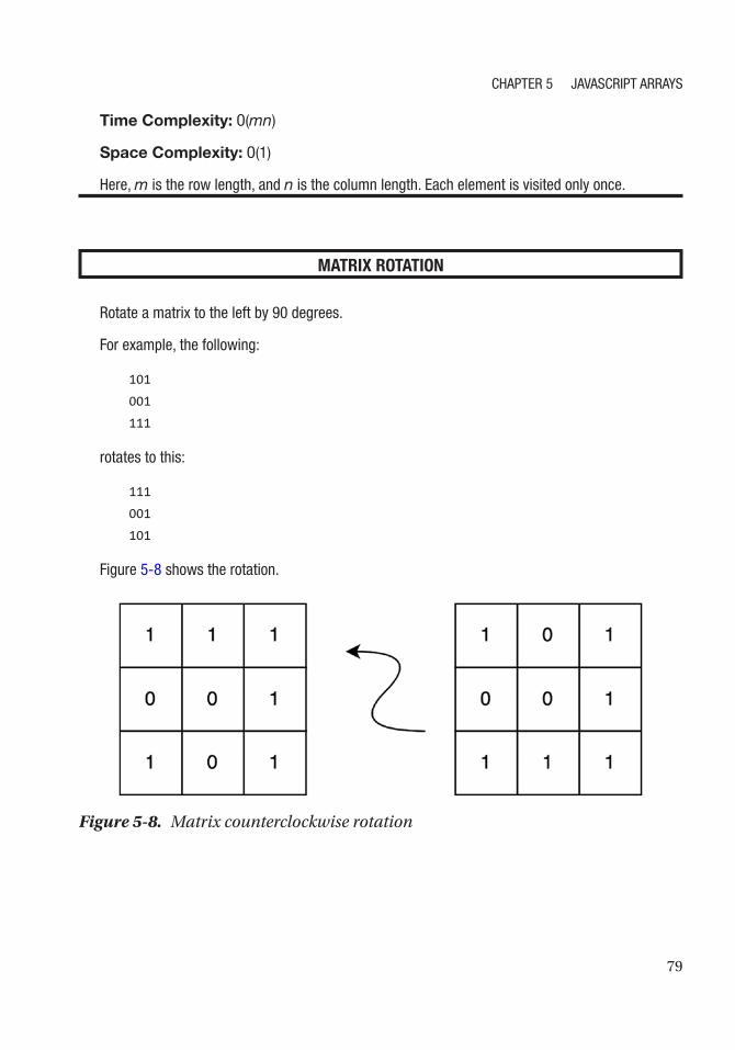
79
Time Complexity: O(mn)
Space Complexity: O(1)
here, m is the row length, and n is the column length. each element is visited only once.
MATRIX ROTATION
rotate a matrix to the left by 90 degrees.
For example, the following:
101
001
111
rotates to this:
111
001
101
Figure 5-8 shows the rotation.
Figure 5-8. Matrix counterclockwise rotation
Chapter 5 JavaSCript arrayS

80
as shown in Figure 5-8, when rotated 90 degrees left, the following happens:
1. the third column of the matrix becomes the first row of the result.
2. the second column of the matrix becomes the second row of the result.
3. the first column of the matrix becomes the third row of the result.
the following rotation turns the third column of the original:
1 var matrix = [[1,0,1],[0,0,1],[1,1,1]];
2
3
4 function rotateMatrix90Left (mat){
5 var N = mat.length;
6
7 // Consider all squares one by one
8 for (var x = 0; x < N / 2; x++) {
9 // Consider elements in group of 4 in
10 // current square
11 for (var y = x; y < N-x-1; y++) {
12 // store current cell in temp variable
13 var temp = mat[x][y];
14
15 // move values from right to top
16 mat[x][y] = mat[y][N-1-x];
17
18 // move values from bottom to right
19 mat[y][N-1-x] = mat[N-1-x][N-1-y];
20
21 // move values from left to bottom
22 mat[N-1-x][N-1-y] = mat[N-1-y][x];
23
24 // assign temp to left
25 mat[N-1-y][x] = temp;
26 }
27 }
28 }
29 rotateMatrix90Left(matrix);
30 console.log(matrix); // [[1,1,1],[0,0,1],[1,0,1]]
Chapter 5 JavaSCript arrayS

81
Time Complexity: O(mn)
Space Complexity: O(1)
here, m is the row length, and n is the column length. each element is visited only once.
the space complexity is O(1) because the original array is modified instead of creating a
new array.
SummaryVarious natively implemented array functions were covered in this chapter and are
summarized in Table 5-1.
In addition to the standard while and for loop mechanisms, an iteration of array
elements can use the alternative loop mechanisms shown in Table 5-2.
Table 5-1. Array Function Summary
Function Usage
push(element) adds an element to the end of the array
pop() removes the last element of the array
shift() removes the first element of the array
slice(beginIndex, endIndex) returns a part of the array from beginIndex to endIndex
splice(beginIndex, endIndex) returns a part of the array from beginIndex to endIndex
and modifies the original array by removing those elements
concat(arr) adds new elements (from arr) into the array at the end
of array
Chapter 5 JavaSCript arrayS

82
Finally, recall that JavaScript utilizes jagged arrays, an array of arrays, to get
multidimensional array behavior. With two-dimensional arrays, two-dimensional
surfaces such as a tic-tac-toe board and maze can easily be represented.
Table 5-2. Iteration Summary
Function Usage
for (var prop in arr) iterates by the index of the array element
for (var elem of arr) iterates by the value of the array element
arr.forEach(fnc) applies the fnc value on each element
Chapter 5 JavaSCript arrayS

83© Sammie Bae 2019 S. Bae, JavaScript Data Structures and Algorithms, https://doi.org/10.1007/978-1-4842-3988-9_6
CHAPTER 6
JavaScript ObjectsJavaScript objects are what makes the JavaScript programming language so versatile.
Before diving into data structures and algorithms, let’s review how JavaScript objects
work. This chapter will focus on what JavaScript objects are, how they are declared, and
how their properties can be changed. In addition, this chapter will cover how JavaScript
classes are implemented using prototypal inheritance.
JavaScript Object PropertyJavaScript objects can be created via the object literal {} or via the syntax new
Object();. Additional properties can be added or accessed in one of two ways: object.
propertyName or object['propertyName'].
1 var javaScriptObject = {};
2 var testArray = [1,2,3,4];
3
4 javaScriptObject.array = testArray;
5 console.log(javaScriptObject); // {array: [1,2,3,4]}
6
7 javaScriptObject.title = 'Algorithms';
8 console.log(javaScriptObject); // {array: [1,2,3,4],
title:'Algorithms'}
As shown in the previous code, the title property was dynamically added in line 7
to the JavaScript object. Similarly, functions in JavaScript classes are added this way by
dynamically adding them to the object.

84
Prototypal InheritanceIn most strongly typed languages such as Java, the methods of a class are defined at
the same time as the class. However, in JavaScript, the function has to be added as a
JavaScript Object property of that class.
Here is an example of a class in JavaScript using this.functionName = function(){}:
1 function ExampleClass(){
2 this.name = "JavaScript";
3 this.sayName = function(){
4 console.log(this.name);
5 }
6 }
7
8 //new object
9 var example1 = new ExampleClass();
10 example1.sayName(); //"JavaScript"
This class dynamically adds the sayName function in the constructor. This pattern is
known as prototypal inheritance.
Prototypal inheritance is the only method of inheritance in JavaScript. To add
functions of a class, simply use the .prototype property and specify the name of
function.
When you use the .prototype property, you are essentially dynamically extending
the JavaScript Object property of the object. This is the standard because JavaScript is
dynamic and classes can add new function members as needed later. This isn’t possible
for compiled languages such as Java because they will throw an error on compilation.
This unique property of JavaScript lets developers take advantage of the prototypical
inheritance.
Here’s an example of using .prototype:
1 function ExampleClass(){
2 this.array = [1,2,3,4,5];
3 this.name = "JavaScript";
4 }
5
Chapter 6 JavaSCript ObJeCtS

85
6 //new object
7 var example1 = new ExampleClass();
8
9 ExampleClass.prototype.sayName = function() {
10 console.log(this.name);
11 }
12
13 example1.sayName(); //"JavaScript"
To reiterate, adding functions to a class dynamically is how JavaScript implements
prototypical inheritance. Functions of a class are added either in the constructor or via
.prototype.
Constructor and VariablesBecause variables of a class in JavaScript are properties of that class object, any
properties declared with this.propertyName will be available publicly. This means that
the object’s properties can be directly accessed in other scopes.
1 function ExampleClass(name, size){
2 this.name = name;
3 this.size = size;
4 }
5
6 var example = new ExampleClass("Public",5);
7 console.log(example); // {name:"Public", size: 5}
8
9 // accessing public variables
10 console.log(example.name); // "Public"
11 console.log(example.size); // 5
To mimic a private variable, instead of using this.propertyName, you can declare
a local variable and have getter/setters that allow access to that variable. This way, the
variable is available only to the constructor’s scope. Notably, however, these mimicked
private variables are now accessible only through the defined interfacing functions
(getter getName and setter setName). These getters and setters cannot be added outside
of the constructor.
Chapter 6 JavaSCript ObJeCtS

86
1 function ExampleClass(name, size) {
2 var privateName = name;
3 var privateSize = size;
4
5 this.getName = function() {return privateName;}
6 this.setName = function(name) {privateName = name;}
7
8 this.getSize = function() {return privateSize;}
9 this.setSize = function(size) {privateSize = size;}
10 }
11
12 var example = new ExampleClass("Sammie",3);
13 example.setSize(12);
14 console.log(example.privateName); // undefined
15 console.log(example.getName()); // "Sammie"
16 console.log(example.size); // undefined
17 console.log(example.getSize()); // 3
SummaryIn JavaScript, unlike other object-oriented programming languages, prototypical
inheritance is the preferred method of inheritance. Prototypical inheritance works by
adding new functions to a JavaScript class via .prototype. Private variables are explicitly
declared in Java and C++. However, a private variable is not supported in JavaScript,
and to mimic the functionality of a private variable, you need to create a variable that
is scoped to the constructor function. Declaring a variable as part of that object in the
constructor via this.variableName automatically makes that property public.
Chapter 6 JavaSCript ObJeCtS
87
Exercises
ADDING A PROPERTY TO AN OBJECT
add an exampleKey property to an empty JavaScript object in two different ways and set it to
exampleValue.
as discussed earlier in this chapter, a property can be added to an object in two ways. there is
no performance advantage or disadvantage of using one way over the other; the choice comes
down to style.
1 var emptyJSObj = {};
2 emptyJSObj['exampleKey'] = 'exampleValue';
3 emptyJSObj.exampleKey = 'exampleValue';
DEFINING CLASSES
Create two classes: Animal and Dog. the Animal class should take two parameters in the
constructor (name and animalType). Set them as its public properties.
in addition, the Animal class should have two functions: sayName and sayAnimalType.
sayName prints name, and sayAnimalType prints animalType initialized in the constructor.
Finally, the Dog class inherits from the Animal class.
1. Let’s first define the Animal class and the specified required functions.
1 function Animal(name, animalType) {
2 this.name = name;
3 this.animalType = animalType;
4 }
5 Animal.prototype.sayName = function () {
6 console.log(this.name);
7 }
8 Animal.prototype.sayAnimalType = function () {
9 console.log(this.animalType);
10 }
Chapter 6 JavaSCript ObJeCtS

88
2. For the Dog class to inherit this, define the Dog class and then copy its
prototype, as shown in the following code block:
1 function Dog(name) {
2 Animal.call(this, name, "Dog");
3 }
4 // copy over the methods
5 Dog.prototype = Object.create(Animal.prototype);
6 var myAnimal = new Animal("ditto", "pokemon");
7 myAnimal.sayName(); // "ditto"
8 myAnimal.sayAnimalType(); // "pokemon"
9 var myDog = new Dog("candy", "dog");
10 myDog.sayName(); // "candy"
11 myDog.sayAnimalType(); // "dog"
Chapter 6 JavaSCript ObJeCtS

89© Sammie Bae 2019 S. Bae, JavaScript Data Structures and Algorithms, https://doi.org/10.1007/978-1-4842-3988-9_7
CHAPTER 7
JavaScript Memory ManagementIn any program, a variable takes up some memory. In low-level programming languages
such as C, the programmer must allocate and deallocate memory manually. In contrast,
the V8 JavaScript engine and other modern JavaScript engines have garbage collectors
that delete unused variables for the programmer. Despite this memory management
done by the JavaScript engine, however, there are common pitfalls that developers
can fall into. This chapter will show some basic examples of these pitfalls and present
techniques to help the garbage collector minimize the key JavaScript memory problems.
Memory LeaksA memory leak is a failure in a program to release discarded memory, causing impaired
performance and sometimes even failure. Memory leaks can happen when JavaScript
engines’ garbage collectors do not free memory properly.
Follow the key principles outlined in this chapter to avoid memory leaks during
JavaScript development.
Reference to an ObjectIf there is a reference to an object, it is in memory. In this example, say that the memory()
function returns some array with 5KB of data.
1 var foo = {
2 bar1: memory(), // 5kb
3 bar2: memory() // 5kb
4 }
5

90
6 function clickEvent(){
7 alert(foo.bar1[0]);
8 }
You might expect the clickEvent() function to use 5KB of memory since it is only
referencing bar1 from the foo object. However, the truth is that it is using 10KB of
memory since it has to load the whole foo object into the function’s into scope to access
the bar1 property.
Leaking DOMIf a variable pointing to a DOM element is declared outside of an event callback, then it
is in memory and leaks DOM if the element is deleted.
In this example, there are two DOM elements selected by document.
getElementByID.
1 <div id="one">One</div>
2 <div id="two">Two</div>
The following JavaScript code demonstrates the DOM memory leak. When one is
clicked, it removes two. When one is clicked again, it still tries to reference the removed
two.
1 var one = document.getElementById("one");
2 var two = document.getElementById("two");
3 one.addEventListener('click', function(){
4 two.remove();
5 console.log(two); // will print the html even after deletion
6 });
The event listener on the one element will cause the two to disappear from the web
page when clicked. However, even if the DOM is deleted in the HTML, reference to it will
remain if used in an event callback. When the two element is no longer in use, this is a
memory leak and should be avoided.
Chapter 7 JavaSCript MeMory ManageMent

91
This can easily be fixed so that it won’t cause a memory leak, as shown here:
1 var one = document.getElementById("one");
2
3 one.addEventListener('click', function(){
4 var two = document.getElementById("two");
5 two.remove();
6 });
Another way to address this is by unregistering the click handler once it has been
used, as shown here:
1 var one = document.getElementById("one");
2 function callBackExample() {
3 var two = document.getElementById("two");
4 two.remove();
5 one.removeEventListener("click",callBackExample);
6 }
7 one.addEventListener("click",callBackExample);
8 });
Global window ObjectIf an object is on the global window object, it is in memory. The window object is a
global object in a browser and comes with various built-in methods such as alert()
and setTimeout(). Any additional objects declared as a property of window will not be
cleared because window is a required object for the browser to run. Remember that any
global variable declared will be set as a property of the window object.
In this example, there are two global variables declared.
1 var a = "apples"; //global with var
2 b = "oranges"; //global without var
3
4 console.log(window.a); // prints "apples"
5 console.log(window.b); // prints "oranges"
It is good to avoid global variables whenever possible. This will help save memory.
Chapter 7 JavaSCript MeMory ManageMent

92
Limiting Object ReferencesAn object is cleared when all references are cleared. Always remember to limit the
amount of scope the function pulls and pass the property of an object only into functions
instead of the entire object. This is because the object’s memory footprint can be very
large (e.g., an array of 100,000 integers for data visualization project); if only one of the
object’s properties is needed, you should avoid using the entire object as a parameter.
For example, do not do this:
1 var test = {
2 prop1: 'test'
3 }
4
5 function printProp1(test){
6 console.log(test.prop1);
7 }
8
9 printProp1(test); //'test'
Instead, pass the property like this:
1 var test = {
2 prop1: 'test'
3 }
4
5 function printProp1(prop1){
6 console.log(prop1);
7 }
8
9 printProp1(test.prop1); //'test'
The delete OperatorAlways remember that the delete operator can be used to delete an unwanted object
property (though it does not work on nonobjects).
1 var test = {
2 prop1: 'test'
Chapter 7 JavaSCript MeMory ManageMent

93
3 }
4 console.log(test.prop1); // 'test'
5 delete test.prop1;
6 console.log(test.prop1); // _undefined_
SummaryAlthough memory in JavaScript is not allocated by the programmer, there are still
numerous ways to mitigate memory leaks where applicable. If the object is in reference,
it is in memory. Similarly, HTML DOM elements should not be referenced once deleted.
Finally, only reference objects in a function that are needed. In many cases, it is more
applicable to pass in a property of the object rather than the object itself. Also, be
extremely mindful when declaring a global variable.
ExercisesIn this chapter, exercises are about identifying memory inefficiencies and optimizing a
given piece of code.
ANALYZING AND OPTIMIZING A PROPERTY CALL
analyze and optimize the call for printProperty.
1 function someLargeArray() {
2 return new Array(1000000);
3 }
4 var exampleObject = {
5 'prop1': someLargeArray(),
6 'prop2': someLargeArray()
7 }
8 function printProperty(obj){
9 console.log(obj['prop1']);
10 }
11 printProperty(exampleObject);
Chapter 7 JavaSCript MeMory ManageMent

94
Problem: an excessive amount of memory is used in printProperty because the entire
object is brought into the printProperty function. to fix this, only the property being printed
should be brought in as a parameter of the function.
Answer:
1 function someLargeArray() {
2 return new Array(1000000);
3 }
4 var exampleObject = {
5 'prop1': someLargeArray(),
6 'prop2': someLargeArray()
7 }
8 function printProperty(prop){
9 console.log(prop);
10 }
11 printProperty(exampleObject['prop1']);
ANALYZING AND OPTIMIZING SCOPE
analyze and optimize the global scope for the following code block:
1 var RED = 0,
2 GREEN = 1,
3 BLUE = 2;
4
5 function redGreenBlueCount(arr) {
6 var counter = new Array(3) .fill(0);
7 for (var i=0; i < arr.length; i++) {
8 var curr = arr[i];
9 if (curr == RED) {
10 counter[RED]++;
11 } else if (curr == GREEN) {
12 counter[GREEN]++;
13 } else if (curr == BLUE) {
14 counter[BLUE]++;
15 }
Chapter 7 JavaSCript MeMory ManageMent
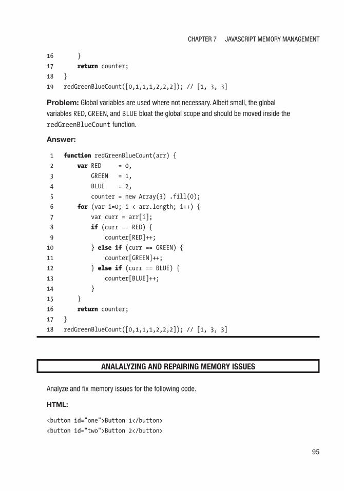
95
16 }
17 return counter;
18 }
19 redGreenBlueCount([0,1,1,1,2,2,2]); // [1, 3, 3]
Problem: global variables are used where not necessary. albeit small, the global
variables RED, GREEN, and BLUE bloat the global scope and should be moved inside the
redGreenBlueCount function.
Answer:
1 function redGreenBlueCount(arr) {
2 var RED = 0,
3 GREEN = 1,
4 BLUE = 2,
5 counter = new Array(3) .fill(0);
6 for (var i=0; i < arr.length; i++) {
7 var curr = arr[i];
8 if (curr == RED) {
9 counter[RED]++;
10 } else if (curr == GREEN) {
11 counter[GREEN]++;
12 } else if (curr == BLUE) {
13 counter[BLUE]++;
14 }
15 }
16 return counter;
17 }
18 redGreenBlueCount([0,1,1,1,2,2,2]); // [1, 3, 3]
ANALALYZING AND REPAIRING MEMORY ISSUES
analyze and fix memory issues for the following code.
HTML:
<button id="one">Button 1</button>
<button id="two">Button 2</button>
Chapter 7 JavaSCript MeMory ManageMent
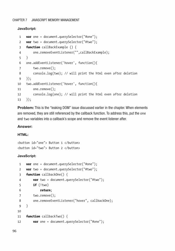
96
JavaScript:
1 var one = document.querySelector("#one");
2 var two = document.querySelector("#two");
3 function callBackExample () {
4 one.removeEventListener("",callBackExample);
5 }
6 one.addEventListener('hover', function(){
7 two.remove();
8 console.log(two); // will print the html even after deletion
9 });
10 two.addEventListener('hover', function(){
11 one.remove();
12 console.log(one); // will print the html even after deletion
13 });
Problem: this is the “leaking DoM” issue discussed earlier in the chapter. When elements
are removed, they are still referenced by the callback function. to address this, put the one
and two variables into a callback’s scope and remove the event listener after.
Answer:
HTML:
<button id="one"> Button 1 </button>
<button id="two"> Button 2 </button>
JavaScript:
1 var one = document.querySelector("#one");
2 var two = document.querySelector("#two");
3 function callbackOne() {
4 var two = document.querySelector("#two");
5 if (!two)
6 return;
7 two.remove();
8 one.removeEventListener("hover", callbackOne);
9 }
10
11 function callbackTwo() {
12 var one = document.querySelector("#one");
Chapter 7 JavaSCript MeMory ManageMent

97
13 if (!one)
14 return;
15 one.remove();
16 two.removeEventListener("hover", callbackTwo);
17 }
18 one.addEventListener("click", callbackOne);
19 two.addEventListener("click", callbackTwo);
Chapter 7 JavaSCript MeMory ManageMent
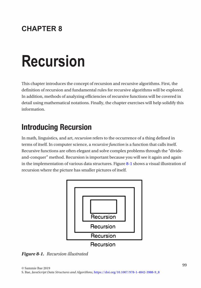
99© Sammie Bae 2019 S. Bae, JavaScript Data Structures and Algorithms, https://doi.org/10.1007/978-1-4842-3988-9_8
CHAPTER 8
RecursionThis chapter introduces the concept of recursion and recursive algorithms. First, the
definition of recursion and fundamental rules for recursive algorithms will be explored.
In addition, methods of analyzing efficiencies of recursive functions will be covered in
detail using mathematical notations. Finally, the chapter exercises will help solidify this
information.
Introducing RecursionIn math, linguistics, and art, recursion refers to the occurrence of a thing defined in
terms of itself. In computer science, a recursive function is a function that calls itself.
Recursive functions are often elegant and solve complex problems through the “divide-
and- conquer” method. Recursion is important because you will see it again and again
in the implementation of various data structures. Figure 8-1 shows a visual illustration of
recursion where the picture has smaller pictures of itself.
Figure 8-1. Recursion illustrated

100
Rules of RecursionWhen recursive functions are implemented incorrectly, it causes fatal issues because the
program will get stuck and not terminate. Infinite recursive calls result in stack overflow.
Stack overflow is when the maximum number of call stacks of the program exceeds the
limited amount of address space (memory).
For recursive functions to be implemented correctly, they must follow certain rules
so that stack overflow is avoided. These rules are covered next.
Base CaseIn recursion, there must be a base case (also referred to as terminating case). Because
recursive methods call themselves, they will never stop unless this base case is reached.
Stack overflow from recursion is most likely the result of not having a proper base case.
In the base case, there are no recursive function calls.
Let’s examine the following function, which prints numbers counting down from n to
0 as an example:
1 function countDownToZero(n) {
2 // base case. Stop at 0
3 if (n < 0) {
4 return; // stop the function
5 } else {
6 console.log(n);
7 countDownToZero(n - 1); // count down 1
8 }
9 }
10 countDownToZero(12);
The base case for this function is when n is smaller or equal to 0. This is because the
desired outcome was to stop counting at 0. If a negative number is given as the input,
it will not print that number because of the base case. In addition to a base case, this
recursive function also exhibits the divide-and-conquer method.
Chapter 8 reCursion

101
Divide-and-Conquer MethodIn computer science, the divide-and-conquer method is when a problem is solved by
solving all of its smaller components. With the countdown example, counting down from
2 can be solved by printing 2 and then counting down from 1. Here, counting down from 1
is the part solved by “dividing and conquering.” It is necessary to make the problem
smaller to reach the base case. Otherwise, if the recursive call does not converge to a
base case, a stack overflow occurs.
Let’s now examine a more complex recursive function known as the Fibonacci
sequence.
Classic Example: Fibonacci SequenceThe Fibonacci sequence is a list of infinite numbers, each of which is the sum of the past
two terms (starting with 1).
1, 1, 2, 3, 5, 8, 13, 21 …
How might you program something to print the Nth term of the Fibonacci sequence?
Iterative Solution: Fibonacci Sequence
An iterative solution using a for loop may look something like this:
1 function getNthFibo(n) {
2 if ( n <= 1) return n;
3 var sum = 0,
4 last = 1,
5 lastlast = 0;
6
7 for (var i = 1; i < n; i++) {
8 sum = lastlast + last;
9 lastlast = last;
10 last = sum;
11 }
12 return sum;
13 }
Chapter 8 reCursion

102
A for loop can be used to keep track of the last two elements of the Fibonacci
sequence, and its sum yields the Fibonacci number.
Now, how might this be done recursively?
Recursive Solution: Fibonacci
The following shows the recursive solution:
1 function getNthFibo(n) {
2 if (n <= 1) {
3 return n;
4 } else {
5 return getNthFibo(n - 1) + getNthFibo(n - 2);
6 }
7 }
Base case: The base case for the Fibonacci sequence is that the first element is 1.
Divide and conquer: By definition of the Fibonacci sequence, the Nth Fibonacci
number is the sum of the (n-1)th and (n-2)th Fibonacci numbers. However, this
implementation has a time complexity of O(2n), which is discussed in detail later in this
chapter. We will explore a more efficient recursive algorithm for the Fibonacci sequence
using tail recursion in the next section.
Fibonacci Sequence: Tail RecursionA tail recursive function is a recursive function in which the recursive call is the last
executed thing in the function. First let’s look at the iterative solution:
1 function getNthFibo(n) {
2 if ( n <= 1) return n;
3 var sum = 0,
4 last = 1,
5 lastlast = 0;
6
7 for (var i = 1; i < n; i++) {
8 sum = lastlast + last;
9 lastlast = last;
Chapter 8 reCursion

103
10 last = sum;
11 }
12 return sum;
13 }
At each iteration, the following update happens: (lastlast, last) = (last,
lastlast+last). With this structure, the following recursive function can be formed:
1 function getNthFiboBetter(n, lastlast, last) {
2 if (n == 0) {
3 return lastlast;
4 }
5 if (n == 1) {
6 return last;
7 }
8 return getNthFiboBetter(n-1, last, lastlast + last);
9 }
Time Complexity: O(n)
At most, this function executes n times because it’s decremented by n-1 each time
with only single recursive call.
Space Complexity: O(n)
The space complexity is also O(n) because of the stack call used for this function.
This will be further explained in the “Recursive Call Stack Memory” section later in this
chapter.
To conclude the rules of recursion, let’s examine another example, which is more
complex.
Pascal’s TriangleIn this example, a function for calculating a term of Pascal’s triangle will be explored.
Pascal’s triangle is a triangle whose element value is the summation of its top two (left
and right) values, as shown in Figure 8-2.
Chapter 8 reCursion

104
Base case: The base case for Pascal’s triangle is that the top element (row=1, col=1)
is 1. Everything else is derived from this fact alone. Hence, when the column is 1, return 1,
and when the row is 0, return 0.
Divide and conquer: By the mathematical definition of Pascal’s triangle, a term of
Pascal’s triangle is defined as the sum of its upper terms. Therefore, this can be expressed as
the following: pascalTriangle(row - 1, col) + pascalTriangle(row - 1, col - 1).
1 function pascalTriangle(row, col) {
2 if (col == 0) {
3 return 1;
4 } else if (row == 0) {
5 return 0;
6 } else {
7 return pascalTriangle(row - 1, col) + pascalTriangle(row - 1,
col - 1);
8 }
Figure 8-2. Pascal’s triangle
Chapter 8 reCursion

105
9 }
10 pascalTriangle(5, 2); // 10
This is the beauty of recursion! Look next at how short and elegant this code is.
Big-O for RecursionIn Chapter 1, Big-O analysis of recursive algorithms was not covered. This was because
recursive algorithms are much harder to analyze. To perform Big-O analysis for recursive
algorithms, its recurrence relations must be analyzed.
Recurrence RelationsIn algorithms implemented iteratively, Big-O analysis is much simpler because loops
clearly define when to stop and how much to increment in each iteration. For analyzing
recursive algorithms, recurrence relations are used. Recurrence relations consist of two-
part analysis: Big-O for base case and Big-O for recursive case.
Let’s revisit the naive Fibonacci sequence example:
function getNthFibo(n) {
if (n <= 1) {
return n;
} else {
return getNthFibo(n - 1) + getNthFibo(n - 2);
}
}
getNthFibo(3);
The base case has a time complexity of O(1). The recursive case calls itself twice.
Let’s represent this as T (n) = T (n − 1) + T (n − 2) + O(1).
• Base case: T (n) = O(1)
• Recursive case: T (n) = T (n − 1) + T (n − 2) + O(1)
Now, this relation means that since T (n) = T (n − 1) + T (n − 2) + O(1), then (by
replacing n with n−1), T (n − 1) = T (n − 2) + T (n − 3) + O(1). Replacing n−1 with n−2
yields T (n − 2) = T (n − 3) + T (n − 4) + O(1). Therefore, you can see that for every call,
there are two more calls for each call. In other words, this has a time complexity of O(2n).
Chapter 8 reCursion

106
It helps to visualize it as such:
F(6) * <-- only once
F(5) *
F(4) **
F(3) ****
F(2) ********
F(1) **************** <-- 16
F(0) ******************************** <-- 32
Calculating Big-O this way is difficult and prone to error. Thankfully, there is a
concept known as the master theorem to help. The master theorem helps programmers
easily analyze the time and space complexities of recursive algorithms.
Master TheoremThe master theorem states the following:
Given a recurrence relation of the form T (n) = aT (n/b) + O(nc)
where a >= 1 and b >=1, there are three cases.
a is the coefficient that is multiplied by the recursive call. b is the “logarithmic” term,
which is the term that divides the n during the recursive call. Finally, c is the polynomial
term on the nonrecursive component of the equation.
The first case is when the polynomial term on the nonrecursive component O(nc) is
smaller than logb(a).
Case 1: c < logb(a) then T (n) = O(n(logb(a))).
For example, T (n) = 8T (n/2) + 1000n2
Identify a, b, c: a = 8, b = 2, c = 2
Evaluate: log2(8) = 3. c < 3 is satisfied.
Result: T (n) = O(n3)
The second case is when c is equal to logb(a).
Case 2: c = logb(a) then T (n) = O(nclog(n)).
For example, T (n) = 2T (n/2) + 10n.
Chapter 8 reCursion

107
Identify a, b, c: a = 2, b = 2, c = 1
Evaluate: log2(2) = 1. c = 1 is satisfied.
Result: T (n) = O(nclog(n)) = T (n) = O(n1log(n)) = T (n) = O(nlog(n))
The third and final case is when c is greater than logb(a).
Case 3: c > logb(a) then T (n) = O(f (n)).
For example, T (n) = 2T (n/2) + n2.
Identify a,b,c: a = 2, b = 2, c = 2
Evaluate: log2(2) = 1. c > 1 is satisfied.
Result: T (n) = f (n) = O(n2)
This section covered a lot about analyzing the time complexity of recursive
algorithms. Space complexity analysis is just as important. The memory used by
recursive function calls should also be noted and analyzed for space complexity
analysis.
Recursive Call Stack MemoryWhen a recursive function calls itself, that takes up memory, and this is really important
in Big-O space complexity analysis.
For example, this simple function for printing from n to 1 recursively takes O(n) in
space:
1 function printNRecursive(n) {
2 console.log(n);
3 if (n > 1){
4 printNRecursive(n-1);
5 }
6 }
7 printNRecursive(10);
A developer can run this on a browser or any JavaScript engine and will see the result
shown in Figure 8-3 in the call stack.
Chapter 8 reCursion
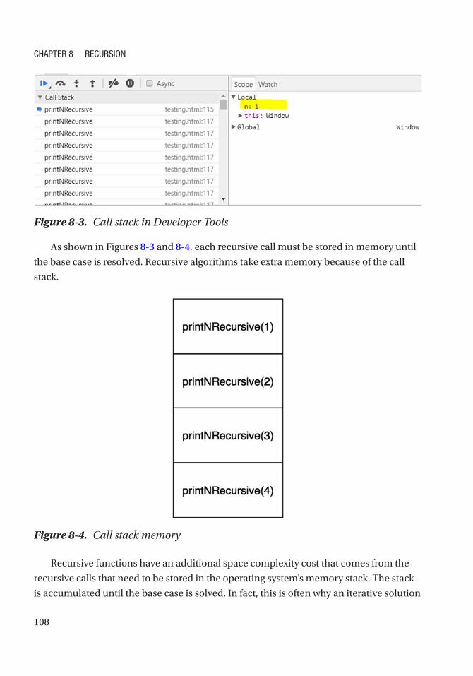
108
As shown in Figures 8-3 and 8-4, each recursive call must be stored in memory until
the base case is resolved. Recursive algorithms take extra memory because of the call
stack.
Recursive functions have an additional space complexity cost that comes from the
recursive calls that need to be stored in the operating system’s memory stack. The stack
is accumulated until the base case is solved. In fact, this is often why an iterative solution
Figure 8-3. Call stack in Developer Tools
Figure 8-4. Call stack memory
Chapter 8 reCursion

109
may be preferred over the recursive solution. In the worst case, if the base case is
implemented incorrectly, the recursive function will cause the program to crash because
of a stack overflow error that occurs when there are more than the allowed number of
elements in the memory stack.
SummaryRecursion is a powerful tool to implement complex algorithms. Recall that all recursive
functions consist of two parts: the base case and the divide-and-conquer method
(solving subproblems).
Analyzing the Big-O of these recursive algorithms can be done empirically (not
recommended) or by using the master theorem. Recall that the master theorem needs
the recurrence relation in the following form: T (n) = aT (n/b) +O(nc). When using the
master theorem, identify a, b, and c to determine which of the three cases of the master
theorem it belongs to.
Finally, when implementing and analyzing recursive algorithms, consider the
additional memory caused by the call stack of the recursive function calls. Each recursive
call requires a place in the call stack at runtime; when the call stack accumulate n calls,
then the space complexity of the function is O(n).
ExercisesThese exercises on recursion cover varying problems to help solidify the knowledge
gained from this chapter. The focus should be to identify the correct base case first before
solving the entire problem. You will find all the code for the exercises on GitHub.1
CONVERT DECIMAL (BASE 10) TO BINARY NUMBER
to do this, keep dividing the number by 2 and each time calculate the modulus (remainder)
and division.
Base case: the base case for this problem is when the n is less than 2. When it is less
than 2, it can be only 0 or 1.
1 https://github.com/Apress/js-data-structures-and-algorithms
Chapter 8 reCursion
110
1 function base10ToString(n) {
2 var binaryString = "";
3
4 function base10ToStringHelper(n) {
5 if (n < 2) {
6 binaryString += n;
7 return;
8 } else {
9 base10ToStringHelper(Math.floor(n / 2));
10 base10ToStringHelper(n % 2);
11 }
12 }
13 base10ToStringHelper(n);
14
15 return binaryString;
16 }
17
18 console.log(base10ToString(232)); // 11101000
Time Complexity: O(log2(n))
time complexity is logarithmic because the recursive call divides the n by 2, which makes the
algorithm fast. For example, for n = 8, it executes only three times. For n=1024, it executes
10 times.
Space Complexity: O(log2(n))
PRINT ALL PERMUTATIONS OF AN ARRAY
this is a classical recursion problem and one that is pretty hard to solve. the premise of the
problem is to swap elements of the array in every possible position.
First, let’s draw the recursion tree for this problem (see Figure 8-5).
Chapter 8 reCursion

111
Base case: beginIndex is equal to endIndex.
When this occurs, the function should print the current permutation.
Permutations: We will need a function to swap elements:
1 function swap(strArr, index1, index2) {
2 var temp = strArr[index1];
3 strArr[index1] = strArr[index2];
4 strArr[index2] = temp;
5 }
1 function permute(strArr, begin, end) {
2 if (begin == end) {
3 console.log(strArr);
4 } else {
5 for (var i = begin; i < end + 1; i++) {
6 swap(strArr, begin, i);
7 permute(strArr, begin + 1, end);
8 swap(strArr, begin, i);
9 }
Figure 8-5. Permutation of array recursion tree
Chapter 8 reCursion
112
10 }
11 }
12
13 function permuteArray(strArr) {
14 permute(strArr, 0, strArr.length - 1);
15 }
16
17 permuteArray(["A", "C", "D"]);
18 // ["A", "C", "D"]
19 // ["A", "D", "C"]
20 // ["C", "A", "D"]
21 // ["C", "D", "A"]
22 // ["D", "C", "A"]
23 // ["D", "A", "C"]
Time Complexity: O(n!)
Space Complexity: O(n!)
there are n! permutations, and it creates n! call stacks.
FLATTEN AN OBJECT
Given a Javascript array like this:
1 var dictionary = {
2 'Key1': '1',
3 'Key2': {
4 'a' : '2',
5 'b' : '3',
6 'c' : {
7 'd' : '3',
8 'e' : '1'
9 }
10 }
11 }
Chapter 8 reCursion

113
flatten it into {'Key1': '1', 'Key2.a': '2','Key2.b' : '3', 'Key2.c.d' : '3',
'Key2.c.e' : '1'}, where the child is denoted by . between the parent and child (see
Figure 8-6).
to do this, iterate over any property and recursively check it for child properties, passing in the
concatenated string name.
Base case: the base case for this problem is when input is not an object.
1 function flattenDictionary(dictionary) {
2 var flattenedDictionary = {};
3
4 function flattenDitionaryHelper(dictionary, propName) {
5 if (typeof dictionary != 'object') {
6 flattenedDictionary[propName] = dictionary;
7 return;
8 }
9 for (var prop in dictionary) {
10 if (propName == "){
11 flattenDitionaryHelper(dictionary[prop], propName+prop);
12 } else {
Figure 8-6. Flatten a dictionary recursion tree
Chapter 8 reCursion
114
13 flattenDitionaryHelper(dictionary[prop],
propName+'.'+prop);
14 }
15 }
16 }
17
18 flattenDitionaryHelper(dictionary, ");
19 return flattenedDictionary;
20 }
Time Complexity: O(n)
Space Complexity: O(n)
each property is visited only once and stored once per n properties.
WRITE A PROGRAM THAT RECURSIVELY DETERMINES IF A STRING IS A PALINDROME
a palindrome is a word spelled the same backward and forward such as deified,
racecar, testset, and aibohphobia (the fear of palindromes).
1 function isPalindromeRecursive(word) {
2 return isPalindromeHelper(word, 0, word.length-1);
3 }
4
5 function isPalindromeHelper(word, beginPos, endPos) {
6 if (beginPos >= endPos) {
7 return true;
8 }
9 if (word.charAt(beginPos) != word.charAt(endPos)) {
10 return false;
11 } else {
12 return isPalindromeHelper(word, beginPos + 1, endPos - 1);
13 }
14 }
15
16 isPalindromeRecursive('hi'); // false
17 isPalindromeRecursive('iii'); // true
Chapter 8 reCursion

115
18 isPalindromeRecursive('ii'); // true
19 isPalindromeRecursive('aibohphobia'); // true
20 isPalindromeRecursive('racecar'); // true
the idea behind this one is that with two indexes (one in front and one in back) you check at
each step until the front and back meet.
Time Complexity: O(n)
Space Complexity: O(n)
space complexity here is still o(n) because of the recursive call stack. remember that the call
stack remains part of memory even if it is not declaring a variable or being stored inside a data
structure.
Chapter 8 reCursion

117© Sammie Bae 2019 S. Bae, JavaScript Data Structures and Algorithms, https://doi.org/10.1007/978-1-4842-3988-9_9
CHAPTER 9
SetsThis chapter focuses on working with sets. The concepts of sets from both a
mathematical definition and on the implementation level are described and explored.
Common set operations, as well as their implementations, are covered in great detail.
By end of this chapter, you will understand how to use JavaScript’s native Set object to
utilize set operations.
Introducing SetsSets are one of the most fundamental data structures. The idea of a set is simple: it is a
group of definite, distinct objects. In layman’s terms, in programming, a set is a group of
unordered unique (no duplicate) elements. For example, a set of integers may be {1, 2, 3, 4}.
Within this, its subsets are {}, {1}, {2}, {3}, {4}, {1, 2}, {1, 3}, {1, 4}, {2, 3}, {2, 4}, {3, 4}, {1, 2, 3},
{1, 2, 4}, {1, 3, 4}, and {2, 3, 4}. Sets are important for checking and adding a unique element
in O(1) constant time. The reason that sets have constant time operations is that the
implementations are based on that of hash tables (covered in Chapter 11).
Set is natively supported in JavaScript as follows:
1 var exampleSet = new Set();
The native Set object has only one property: size (integer). This property is the
current number of elements within the set.
Set OperationsThe set is a powerful data structure for performing uniqueness checks. This section will
cover the following key operations: insertion, deletion, and contains.

118
InsertionSet has one primary function: to check for uniqueness. Set can add items, but duplicates
are not allowed.
1 var exampleSet = new Set();
2 exampleSet.add(1); // exampleSet: Set {1}
3 exampleSet.add(1); // exampleSet: Set {1}
4 exampleSet.add(2); // exampleSet: Set {1, 2}
Notice that adding the duplicate element does not work for a set. As discussed in the
introduction, insertion into a set occurs in constant time.
Time Complexity: O(1)
DeletionSet can also delete items from the set. Set.delete returns a boolean (true if that element
exists and was deleted, false otherwise).
1 var exampleSet = new Set();
2 exampleSet.add(1); // exampleSet: Set {1}
3 exampleSet.delete(1); // true
4 exampleSet.add(2); // exampleSet: Set {2}
This is useful for being able to delete items in constant time in contrast to arrays
where it would take O(n) time to delete an item.
Time Complexity: O(1)
ContainsSet.has does a quick O(1) lookup to check whether the element exists within the set.
1 var exampleSet = new Set();
2 exampleSet.add(1); // exampleSet: Set {1}
3 exampleSet.has(1); // true
4 exampleSet.has(2); // false
5 exampleSet.add(2); // exampleSet: Set {1, 2}
6 exampleSet.has(2); // true
Time Complexity: O(1)
Chapter 9 SetS

119
Other Utility FunctionsIn addition to the natively supported set functions, other essential operations are
available; they are explored in this section.
IntersectionFirst, the intersection of two sets consists of the common elements between those two
sets. This function returns a set with common elements between two sets:
1 function intersectSets (setA, setB) {
2 var intersection = new Set();
3 for (var elem of setB) {
4 if (setA.has(elem)) {
5 intersection.add(elem);
6 }
7 }
8 return intersection;
9 }
10 var setA = new Set([1, 2, 3, 4]),
11 setB = new Set([2, 3]);
12 intersectSets(setA,setB); // Set {2, 3}
isSuperSetSecond, a set is a “superset” of another set if it contains all the elements of the other set.
This function checks whether a set is a superset of another. This is implemented simply
by checking whether the other set contains all the elements of the reference set.
1 function isSuperset(setA, subset) {
2 for (var elem of subset) {
3 if (!setA.has(elem)) {
4 return false;
5 }
6 }
7 return true;
8 }
Chapter 9 SetS

120
9 var setA = new Set([1, 2, 3, 4]),
10 setB = new Set([2, 3]),
11 setC = new Set([5]);
12 isSuperset(setA, setB); // true
13 // because setA has all elements that setB does
14 isSuperset(setA, setC); // false
15 // because setA does not contain 5 which setC contains
UnionThird, the union of two sets combines the elements from both sets. This function returns
a new set with both elements without duplicates.
1 function unionSet(setA, setB) {
2 var union = new Set(setA);
3 for (var elem of setB) {
4 union.add(elem);
5 }
6 return union;
7 }
8 var setA = new Set([1, 2, 3, 4]),
9 setB = new Set([2, 3]),
10 setC = new Set([5]);
11 unionSet(setA,setB); // Set {1, 2, 3, 4}
12 unionSet(setA,setC); // Set {1, 2, 3, 4, 5}
DifferenceFinally, the difference of set A from set B is all of the elements in set A that are not in set B.
This function implements the difference operation by making use of the native delete
method.
1 function differenceSet(setA, setB) {
2 var difference = new Set(setA);
3 for (var elem of setB) {
4 difference.delete(elem);
Chapter 9 SetS
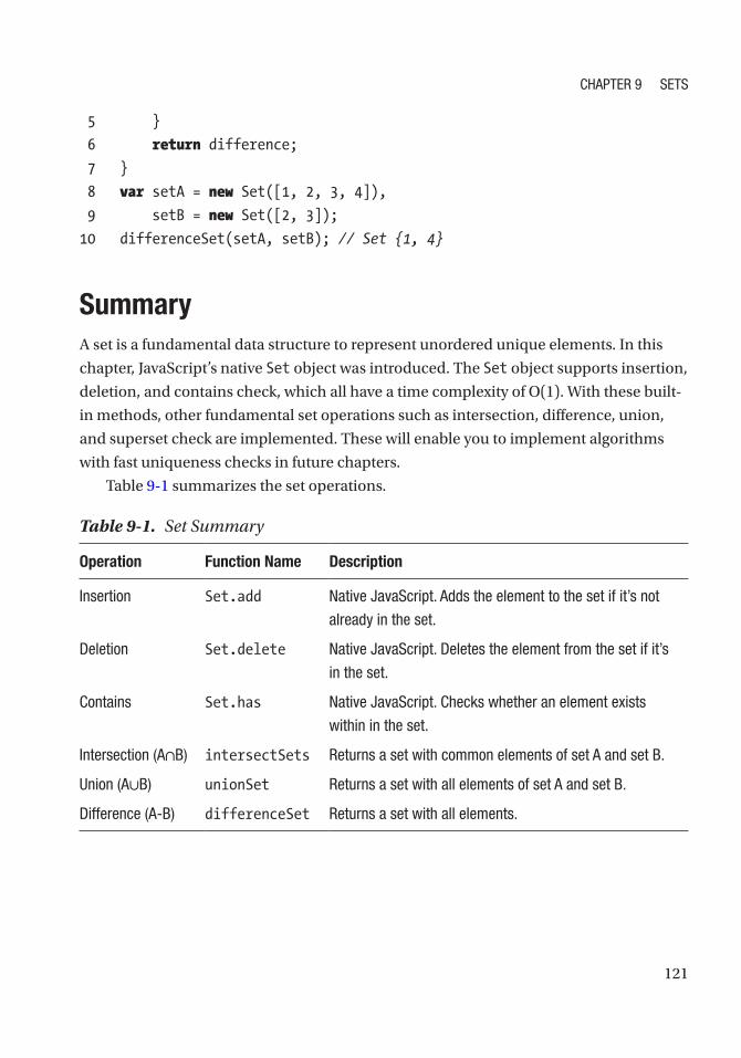
121
5 }
6 return difference;
7 }
8 var setA = new Set([1, 2, 3, 4]),
9 setB = new Set([2, 3]);
10 differenceSet(setA, setB); // Set {1, 4}
SummaryA set is a fundamental data structure to represent unordered unique elements. In this
chapter, JavaScript’s native Set object was introduced. The Set object supports insertion,
deletion, and contains check, which all have a time complexity of O(1). With these built-
in methods, other fundamental set operations such as intersection, difference, union,
and superset check are implemented. These will enable you to implement algorithms
with fast uniqueness checks in future chapters.
Table 9-1 summarizes the set operations.
Table 9-1. Set Summary
Operation Function Name Description
Insertion Set.add Native JavaScript. adds the element to the set if it’s not
already in the set.
Deletion Set.delete Native JavaScript. Deletes the element from the set if it’s
in the set.
Contains Set.has Native JavaScript. Checks whether an element exists
within in the set.
Intersection (a∩B) intersectSets returns a set with common elements of set a and set B.
Union (a∪B) unionSet returns a set with all elements of set a and set B.
Difference (a-B) differenceSet returns a set with all elements.
Chapter 9 SetS
122
Exercises
USING SETS TO CHECK FOR DUPLICATES IN AN ARRAY
Check whether there are any duplicates in an array of integers using sets. By converting the
array into a set, the size of the set can be compared with the length of the array to check for
duplicates easily.
1 function checkDuplicates(arr) {
2 var mySet = new Set(arr);
3 return mySet.size < arr.length;
4 }
5 checkDuplicates([1,2,3,4,5]); // false
6 checkDuplicates([1,1,2,3,4,5]); // true
Time Complexity: O(n)
Space Complexity: O(n)
In an array of length n, this function has to iterate through the entire array in the worst case
and also store all those elements in the set.
RETURNING ALL UNIQUE VALUES FROM SEPARATE ARRAYS
Given two integer arrays with some of the same values, return one array that has all the
unique elements from both of the original arrays.
Using sets, unique elements can be stored easily. By concatenating two arrays and converting
them to a set, only unique items are stored. Converting the set to an array results in an array
with unique items only.
1 function uniqueList(arr1, arr2) {
2 var mySet = new Set(arr1.concat(arr2));
3 return Array.from(mySet);
4 }
5
Chapter 9 SetS

123
6 uniqueList([1,1,2,2],[2,3,4,5]); // [1,2,3,4,5]
7 uniqueList([1,2],[3,4,5]); // [1,2,3,4,5]
8 uniqueList([],[2,2,3,4,5]); // [2,3,4,5]
Time Complexity: O(n + m )
Space Complexity: O(n + m)
the time and space complexity for this algorithm is O(n + m) where n is the length of arr1
and m is the length of arr2. this is because all elements inside both arrays need to be
iterated through.
Chapter 9 SetS
125© Sammie Bae 2019 S. Bae, JavaScript Data Structures and Algorithms, https://doi.org/10.1007/978-1-4842-3988-9_10
CHAPTER 10
Searching and SortingSearching data and sorting through data are fundamental algorithms. Searching refers to
iterating over the data structure’s elements to retrieve some data. Sorting refers to putting
the data structure’s elements in order. The searching and sorting algorithms are different
for every data structure. This chapter focuses on searching and sorting for arrays. By
the end of this chapter, you will understand how to use common sorting and searching
algorithms for arrays.
SearchingAs mentioned, searching is the task of looking for a specific element inside a data
structure. When searching in an array, there are two main techniques depending
on whether the array is sorted. In this section, you’ll learn about linear and binary
searching. Linear searches are especially flexible because they can be used with both
sorted and unsorted data. Binary searches are specifically used with sorted data.
However, a linear search has a higher time complexity than a binary search.
Linear SearchA linear search works by going through each element of the array one index after another
sequentially. The following code example is an implementation of a linear search that
iterates through the entire array of numbers to find out whether 4 and 5 exist within the
array.
1 //iterate through the array and find
2 function linearSearch(array,n){
3 for(var i=0; i<array.length; i++) {
4 if (array[i]==n) {
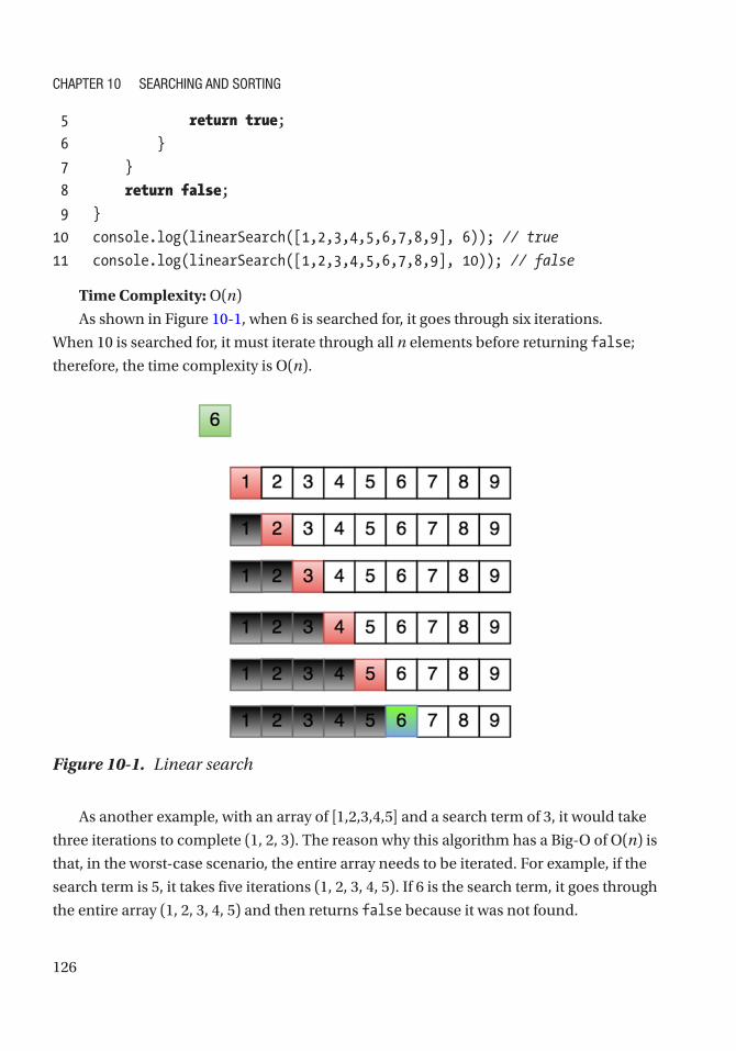
126
5 return true;
6 }
7 }
8 return false;
9 }
10 console.log(linearSearch([1,2,3,4,5,6,7,8,9], 6)); // true
11 console.log(linearSearch([1,2,3,4,5,6,7,8,9], 10)); // false
Time Complexity: O(n)
As shown in Figure 10-1, when 6 is searched for, it goes through six iterations.
When 10 is searched for, it must iterate through all n elements before returning false;
therefore, the time complexity is O(n).
Figure 10-1. Linear search
As another example, with an array of [1,2,3,4,5] and a search term of 3, it would take
three iterations to complete (1, 2, 3). The reason why this algorithm has a Big-O of O(n) is
that, in the worst-case scenario, the entire array needs to be iterated. For example, if the
search term is 5, it takes five iterations (1, 2, 3, 4, 5). If 6 is the search term, it goes through
the entire array (1, 2, 3, 4, 5) and then returns false because it was not found.
Chapter 10 SearChing and Sorting

127
As noted previously, a linear search algorithm like this is great because it works
whether or not the array is sorted. In a linear search algorithm, every element of the
array is checked. So, you should use a linear search when the array is not sorted. If the
array is sorted, you can do the search faster via a binary search.
Binary SearchBinary search is a searching algorithm that works on sorted data. Unlike the linear search
algorithm, in which every element of the array is checked, binary searches can check the
middle value to see whether the desired value is greater or smaller than it. If the desired
value is smaller, this algorithm can search through the smaller parts, or it can search
through the bigger parts if the desired value is bigger.
Figure 10-2 illustrates the process of a binary search. First, the search range is 1 to 9. Since
the middle element, 5, is bigger than 3, the search range is restricted to 1 to 4. Finally, 3 is found
as the middle element. Figure 10-3 illustrates searching for an item in the right half of the array.
Figure 10-2. Binary search in the left half of the array
Figure 10-3. Binary search in the right half of the array
Chapter 10 SearChing and Sorting

128
The following code implements the binary search algorithm described:
1 function binarySearch(array,n){
2 var lowIndex = 0, highIndex = array1.length-1;
3
4 while(lowIndex<=highIndex){
5 var midIndex = Math.floor((highIndex+lowIndex) /2);
6 if (array[midIndex]==n) {
7 return midIndex;
8 } else if (n>array[midIndex]) {
9 lowIndex = midIndex;
10 } else {
11 highIndex = midIndex;
12 }
13 }
14 return -1;
15 }
16 console.log(binarySearch([1,2,3,4], 4)); // true
17 console.log(binarySearch([1,2,3,4], 5)); // -1
The binary search algorithm is fast but can be done only if the array is sorted. It
checks the middle element if that is the element that is being searched for. If the search
element is bigger than the middle element, the lower bound is set to the middle element
plus one. If the search element is less than the middle element, the higher bound is set to
the middle element minus one.
This way, the algorithm is continuously dividing the array into two sections: the
lower half and the upper half. If the element is smaller than the middle element, it
should look for it in the lower half; if the element is bigger than the middle element, it
should look for it in the upper half.
Binary searches are used by humans without them even knowing. An example is a
phone directory that is arranged from A to Z by last name.
If you are given the task of finding someone with the last name of Lezer, one would
first go to the L section and open it halfway through. Lizar is on that page; this means
that the lower section contains L + [a to i] and the upper section contains L + [i to z] last
names. You would then check the middle of the lower section. Laar appears, so you
would now check the upper section. This process repeats until Lezer is found.
Chapter 10 SearChing and Sorting
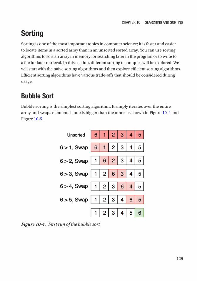
129
SortingSorting is one of the most important topics in computer science; it is faster and easier
to locate items in a sorted array than in an unsorted sorted array. You can use sorting
algorithms to sort an array in memory for searching later in the program or to write to
a file for later retrieval. In this section, different sorting techniques will be explored. We
will start with the naive sorting algorithms and then explore efficient sorting algorithms.
Efficient sorting algorithms have various trade-offs that should be considered during
usage.
Bubble SortBubble sorting is the simplest sorting algorithm. It simply iterates over the entire
array and swaps elements if one is bigger than the other, as shown in Figure 10-4 and
Figure 10-5.
Figure 10-4. First run of the bubble sort
Chapter 10 SearChing and Sorting
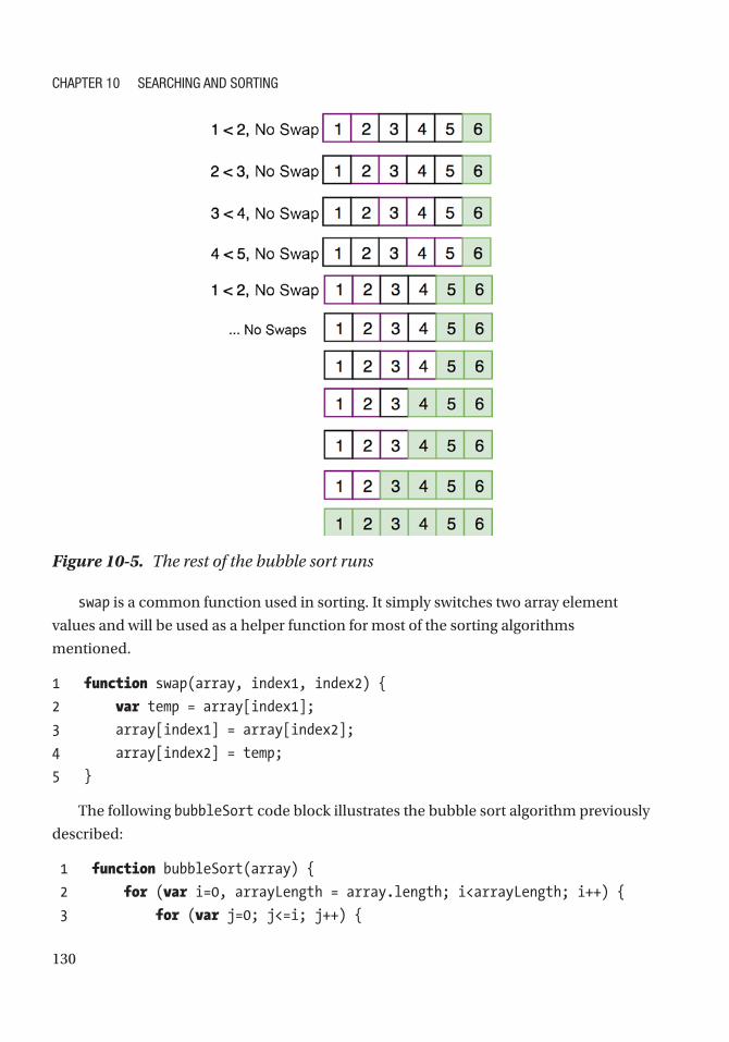
130
swap is a common function used in sorting. It simply switches two array element
values and will be used as a helper function for most of the sorting algorithms
mentioned.
1 function swap(array, index1, index2) {
2 var temp = array[index1];
3 array[index1] = array[index2];
4 array[index2] = temp;
5 }
The following bubbleSort code block illustrates the bubble sort algorithm previously
described:
1 function bubbleSort(array) {
2 for (var i=0, arrayLength = array.length; i<arrayLength; i++) {
3 for (var j=0; j<=i; j++) {
Figure 10-5. The rest of the bubble sort runs
Chapter 10 SearChing and Sorting

131
4 if (array[i] < array[j]) {
5 swap(array, i, j);
6 }
7 }
8 }
9 return array;
10 }
11 bubbleSort([6,1,2,3,4,5]); // [1,2,3,4,5,6]
Time Complexity: O(n2)
Space Complexity: O(1)
Bubble sort is the worst type of sort because it compares every pair possible, whereas
other sorting algorithms take advantage of the presorted parts of the array. Because
bubble sort uses nested loops, it has a time complexity of O(n2).
Selection SortSelection sorting works by scanning the elements for the smallest element and inserting
it into the current position of the array. This algorithm is marginally better than bubble
sort. Figure 10-6 shows this minimum selection process.
Figure 10-6. Selection sort
Chapter 10 SearChing and Sorting

132
The following code implements the selection sort. In the code, there is one for loop to
iterate through the array and one nested for loop to scan to get the minimum element.
1 function selectionSort(items) {
2 var len = items.length,
3 min;
4
5 for (var i=0; i < len; i++){
6 // set minimum to this position
7 min = i;
8 //check the rest of the array to see if anything is smaller
9 for (j=i+1; j < len; j++){
10 if (items[j] < items[min]){
11 min = j;
12 }
13 }
14 //if the minimum isn't in the position, swap it
15 if (i != min){
16 swap(items, i, min);
17 }
18 }
19
20 return items;
21 }
22 selectionSort([6,1,23,4,2,3]); // [1, 2, 3, 4, 6, 23]
Time Complexity: O(n2)
Space Complexity: O(1)
The time complexity for selection sort is still O(n2) because of the nested for loop.
Insertion SortInsertion sort works similarly to selection sort by searching the array sequentially and
moving the unsorted items into a sorted sublist on the left side of the array. Figure 10-7
shows this process in detail.
Chapter 10 SearChing and Sorting

133
The following code implements the insertion sort algorithm. The outer for loop
iterates over the array indices, and the inner for loop moves the unsorted items into the
sorted sublist on the left side of the array.
1 function insertionSort(items) {
2 var len = items.length, // number of items in the array
3 value, // the value currently being compared
4 i, // index into unsorted section
5 j; // index into sorted section
6
7 for (i=0; i < len; i++) {
8 // store the current value because it may shift later
9 value = items[i];
10
11 // Whenever the value in the sorted section is greater than the value
12 // in the unsorted section, shift all items in the sorted section
13 // over by one. This creates space in which to insert the value.
14
Figure 10-7. Insertion sort
Chapter 10 SearChing and Sorting

134
15 for (j=i-1; j > -1 && items[j] > value; j--) {
16 items[j+1] = items[j];
17 }
18 items[j+1] = value;
19 }
20 return items;
21 }
22 insertionSort([6,1,23,4,2,3]); // [1, 2, 3, 4, 6, 23]
Time Complexity: O(n2)
Space Complexity: O(1)
Again, this sorting algorithm has a quadratic time complexity of O(n2) like bubble
and insertion sort because of the nested for loop.
QuicksortQuicksort works by obtaining a pivot and partitioning the array around it (bigger
elements on one side and smaller elements on the other side) until everything is
sorted. The ideal pivot is the median of the array since it will partition the array
evenly but getting the median of an unsorted array linear time to compute. Hence,
a pivot is typically obtained by taking the median value of the first, middle, and last
elements in the partition. This sort is a recursive one and uses the divide-and-conquer
methodology to break the quadratic complexity barrier and get the time complexity
down to O(nlog2(n)). However, with a pivot that partitions everything on one side, the
time complexity is worse case: O(n2).
Figure 10-8 shows the quicksort process’s partitioning steps in great detail.
Chapter 10 SearChing and Sorting

135
The following code shows an implementation of the quicksort algorithm:
1 function quickSort(items) {
2 return quickSortHelper(items, 0, items.length-1);
3 }
4
5 function quickSortHelper(items, left, right) {
6 var index;
7 if (items.length > 1) {
8 index = partition(items, left, right);
9
10 if (left < index - 1) {
Figure 10-8. Quicksort
Chapter 10 SearChing and Sorting

136
11 quickSortHelper(items, left, index - 1);
12 }
13
14 if (index < right) {
15 quickSortHelper(items, index, right);
16 }
17 }
18 return items;
19 }
20
21 function partition(array, left, right) {
22 var pivot = array[Math.floor((right + left) / 2)];
23 while (left <= right) {
24 while (pivot > array[left]) {
25 left++;
26 }
27 while (pivot < array[right]) {
28 right--;
29 }
30 if (left <= right) {
31 var temp = array[left];
32 array[left] = array[right];
33 array[right]= temp;
34 left++;
35 right--;
36 }
37 }
38 return left;
39 }
40
41 quickSort([6,1,23,4,2,3]); // [1, 2, 3, 4, 6, 23]
Time Complexity: O(nlog2(n)) on average, O(n2) for worst case
Space Complexity: O(log2(n))
Chapter 10 SearChing and Sorting

137
One downside about a quicksort algorithm is that it could potentially be O(n2) if a
bad pivot is always picked. A bad pivot is one that it does not partition the array evenly.
The ideal pivot is the median element of the array. In addition, a quicksort algorithm
takes a bigger space complexity of O(log2(n)) compared to other sorting algorithms
because of the call stack in recursion.
Use a quicksort algorithm when the average performance should be optimal. This
has to do with the fact that quicksort works better for the RAM cache.
QuickselectQuickselect is a selection algorithm to find the kth smallest element in an unordered list.
Quickselect uses the same approach as a quicksort algorithm. A pivot is chosen, and the
array is partitioned. Instead of recursing both sides like quicksort, however, it recurses
only the side for the element. This reduces the complexity from O(nlog2(n)) to O(n).
Quickselect is implemented in the following code:
1 var array = [1,3,3,-2,3,14,7,8,1,2,2];
2 // sorted form: [-2, 1, 1, 2, 2, 3, 3, 3, 7, 8, 14]
3
4 function quickSelectInPlace(A, l, h, k){
5 var p = partition(A, l, h);
6 if(p==(k-1)) {
7 return A[p];
8 } else if(p>(k-1)) {
9 return quickSelectInPlace(A, l, p - 1,k);
10 } else {
11 return quickSelectInPlace(A, p + 1, h,k);
12 }
13 }
14
15 function medianQuickselect(array) {
16 return quickSelectInPlace(array,0,array.length-1, Math.
floor(array.length/2));
17 }
18
19 quickSelectInPlace(array,0,array.length-1,5); // 2
Chapter 10 SearChing and Sorting

138
20 // 2 - because it's the fifth smallest element
21 quickSelectInPlace(array,0,array.length-1,10); // 7
22 // 7 - because it's the tenth smallest element
Time Complexity: O(n)
MergesortMergesort works by dividing the array into subarrays until each array has one element.
Then, each subarray is concatenated (merged) in a sorted order (see Figure 10-9).
Figure 10-9. Mergesort
The merge function should add all the elements from both arrays in sorted order in a
“result array.” To do this, the index of each array can be created to keep track of elements
already compared. Once one array exhausts all its elements, the rest can be appended to
the result array.
1 function merge(leftA, rightA){
2 var results= [], leftIndex= 0, rightIndex= 0;
3
Chapter 10 SearChing and Sorting

139
4 while (leftIndex < leftA.length && rightIndex < rightA.length) {
5 if( leftA[leftIndex]<rightA[rightIndex] ){
6 results.push(leftA[leftIndex++]);
7 } else {
8 results.push(rightA[rightIndex++]);
9 }
10 }
11 var leftRemains = leftA.slice(leftIndex),
12 rightRemains = rightA.slice(rightIndex);
13
14 // add remaining to resultant array
15 return results.concat(leftRemains).concat(rightRemains);
16 }
The merging function works by taking the two arrays (left and right) and merging
them into one resultant array. The elements need to be compared as they get merged to
preserve order.
Now, the mergeSort function has to partition the bigger array into two separate
arrays and recursively call merge.
1 function mergeSort(array) {
2
3 if(array.length<2){
4 return array; // Base case: array is now sorted since it's
just 1 element
5 }
6
7 var midpoint = Math.floor((array.length)/2),
8 leftArray = array.slice(0, midpoint),
9 rightArray = array.slice(midpoint);
10
11 return merge(mergeSort(leftArray), mergeSort(rightArray));
12 }
13 mergeSort([6,1,23,4,2,3]); // [1, 2, 3, 4, 6, 23]
Time Complexity: O(nlog2(n))
Space Complexity: O(n)
Chapter 10 SearChing and Sorting

140
Mergesort has a large space complexity of O(n) because of the need to create n number
of arrays to be merged later. Use mergesort when a stable sort is needed. A stable sort is
one that’s guaranteed not to reorder elements with identical keys. Mergesort is guaranteed
to be O(nlog2(n)). A disadvantage of mergesort is that it uses O(n) in space.
Count SortCount sort can be done in O(k+n) because it does not compare values. It works only for
numbers and given a certain range. Instead of sorting by swapping elements, this count
works by counting occurrences of each element in the array. Once occurrences of each
element are counted, the new array can be created using those occurrences. This sorts
the data without having to swap elements, as shown in Figure 10-10.
Figure 10-10. Count sort
Here’s an implementation using a JavaScript object:
1 function countSort(array) {
2 var hash = {}, countArr= [];
3 for(var i=0;i<array.length;i++){
4 if(!hash[array[i]]){
5 hash[array[i]] = 1;
6 }else{
7 hash[array[i]]++;
8 }
9 }
10
Chapter 10 SearChing and Sorting

141
11 for(var key in hash){
12 // for any number of _ element, add it to array
13 for(var i=0;i<hash[key];i++) {
14 countArr.push(parseInt(key));
15 }
16 }
17
18 return countArr;
19 }
20 countSort([6,1,23,2,3,2,1,2,2,3,3,1,123,123,4,2,3]); // [1, 2, 3, 4, 6, 23]
Time Complexity: O(k+n)
Space Complexity: O(k)
Use count sort when you’re sorting integers with a limited range. This will be the
fastest sort for this case.
JavaScript’s Built-in SortJavaScript has a built-in sort() method for an array object, which sorts elements
by ascending order. To use it, there is an optional parameter that you can pass in a
comparator function.
However, the default comparator function sorts alphabetically, so it will not work for
numbers.
1 var array1 = [12,3,4,2,1,34,23];
2 array1.sort(); // array1: [1, 12, 2, 23, 3, 34, 4]
In the previous example, notice that numbers starting with 1 came first (1, 12), then
numbers starting with 2, and so forth. This is because no comparator function was passed
and JavaScript converted the elements into a string and sorted it according to the alphabet.
To sort numbers correctly, use this:
1 var array1 = [12,3,4,2,1,34,23];
2
3 function comparatorNumber(a,b) {
4 return a-b;
5 }
6
Chapter 10 SearChing and Sorting
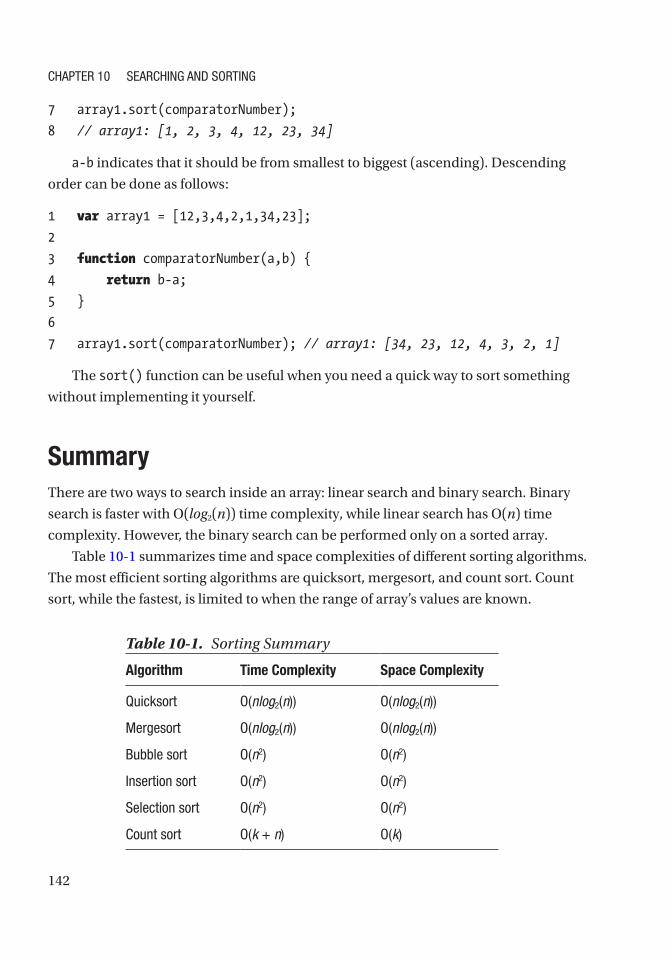
142
7 array1.sort(comparatorNumber);
8 // array1: [1, 2, 3, 4, 12, 23, 34]
a-b indicates that it should be from smallest to biggest (ascending). Descending
order can be done as follows:
1 var array1 = [12,3,4,2,1,34,23];
2
3 function comparatorNumber(a,b) {
4 return b-a;
5 }
6
7 array1.sort(comparatorNumber); // array1: [34, 23, 12, 4, 3, 2, 1]
The sort() function can be useful when you need a quick way to sort something
without implementing it yourself.
SummaryThere are two ways to search inside an array: linear search and binary search. Binary
search is faster with O(log2(n)) time complexity, while linear search has O(n) time
complexity. However, the binary search can be performed only on a sorted array.
Table 10-1 summarizes time and space complexities of different sorting algorithms.
The most efficient sorting algorithms are quicksort, mergesort, and count sort. Count
sort, while the fastest, is limited to when the range of array’s values are known.
Table 10-1. Sorting Summary
Algorithm Time Complexity Space Complexity
Quicksort o(nlog2(n)) o(nlog2(n))
Mergesort o(nlog2(n)) o(nlog2(n))
Bubble sort o(n2) o(n2)
insertion sort o(n2) o(n2)
Selection sort o(n2) o(n2)
Count sort o(k + n) o(k)
Chapter 10 SearChing and Sorting

143
Exercises
USE THE IMPLEMENT SQUARE ROOT FUNCTION FOR AN INTEGER WITHOUT USING ANY MATH LIBRARIES
the first solution that may come to mind is trying every possibility from 1 to the number, as
follows:
1 function sqrtIntNaive(number){
2 if(number == 0 || number == 1)
3 return number;
4
5 var index = 1, square = 1;
6
7 while(square < number){
8 if (square == number){
9 return square;
10 }
11
12 index++;
13 square = index*index;
14 }
15 return index;
16 }
17 sqrtIntNaive(9);
Time Complexity: o(n)
this is essentially a linear search since it has to linearly check one by one the value for the
square root.
the binary search algorithm can be applied to this problem. instead of going up 1 by 1,
partition the range into upper half and lower half between 1 and the given number as follows:
1 function sqrtInt(number) {
2 if(number == 0 || number == 1) return number;
3
4 var start = 1, end = number, ans;
5
Chapter 10 SearChing and Sorting

144
6 while(start <= end) {
7 let mid = parseInt((start+end)/2);
8
9 if (mid*mid == number)
10 return mid;
11
12 if(mid*mid<number){
13 start = mid+1; // use the upper section
14 ans = mid;
15 }else{
16 end = mid-1; // use the lower section
17 }
18 }
19 return ans;
20 }
21 sqrtInt(9);
Time Complexity: o(log2(n))
Bonus: Find a Square Root of a Float
For this exercise, the only difference is using a threshold value to calculate accuracy to because
the square root of a double will have decimals. hence, the time complexity also stays the same.
1 function sqrtDouble(number) {
2 var threshold = 0.1;
3 //9 try middle,
4 var upper = number;
5 var lower = 0;
6 var middle;
7 while(upper-lower>threshold){
8 middle = (upper+lower)/2;
9 if(middle*middle>number){
10 upper = middle;
11 }else{
12 lower = middle;
13 }
14 }
15 return middle
16 }
17 sqrtDouble(9); // 3.0234375
Chapter 10 SearChing and Sorting

145
FIND IF TWO ELEMENTS OF AN ARRAY ADD UP TO A GIVEN NUMBER
the simple approach to this problem is to check every other element for each element in the array.
1 function findTwoSum(array, sum) {
2
3 for(var i=0, arrayLength = array.length; i<arrayLength;i++){
4 for(var j=i+1;j<arrayLength;j++){
5 if(array[j]+array[i] == sum){
6 return true;
7 }
8 }
9 }
10 return false;
11 }
Time Complexity: o(n2)
Space Complexity: o(1)
there is a lot of checking, and hence it takes quadratic time.
a better approach is to store the already visited numbers and check against them. this way, it
can be done in linear time.
1 function findTwoSum(array, sum){
2 var store = {};
3
4 for(var i=0, arrayLength = array.length; i<arrayLength;i++){
5 if(store[array[i]]){
6 return true;
7 }else{
8 store[sum-array[i]] = array[i];
9 }
10 }
11 return false;
12 }
Chapter 10 SearChing and Sorting
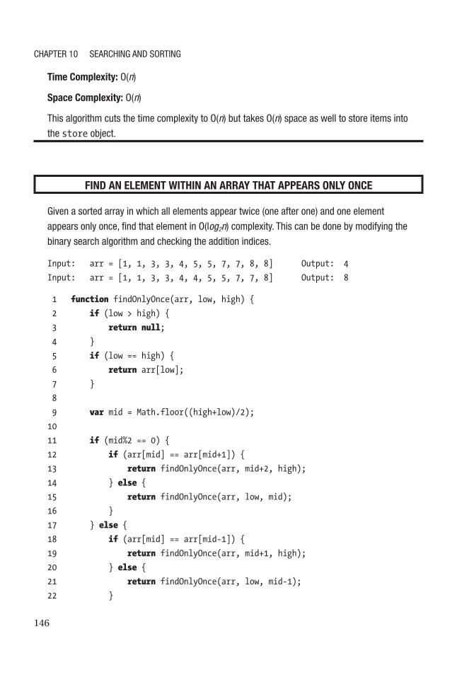
146
Time Complexity: o(n)
Space Complexity: o(n)
this algorithm cuts the time complexity to o(n) but takes o(n) space as well to store items into
the store object.
FIND AN ELEMENT WITHIN AN ARRAY THAT APPEARS ONLY ONCE
given a sorted array in which all elements appear twice (one after one) and one element
appears only once, find that element in o(log2n) complexity. this can be done by modifying the
binary search algorithm and checking the addition indices.
Input: arr = [1, 1, 3, 3, 4, 5, 5, 7, 7, 8, 8] Output: 4
Input: arr = [1, 1, 3, 3, 4, 4, 5, 5, 7, 7, 8] Output: 8
1 function findOnlyOnce(arr, low, high) {
2 if (low > high) {
3 return null;
4 }
5 if (low == high) {
6 return arr[low];
7 }
8
9 var mid = Math.floor((high+low)/2);
10
11 if (mid%2 == 0) {
12 if (arr[mid] == arr[mid+1]) {
13 return findOnlyOnce(arr, mid+2, high);
14 } else {
15 return findOnlyOnce(arr, low, mid);
16 }
17 } else {
18 if (arr[mid] == arr[mid-1]) {
19 return findOnlyOnce(arr, mid+1, high);
20 } else {
21 return findOnlyOnce(arr, low, mid-1);
22 }
Chapter 10 SearChing and Sorting

147
23 }
24 }
25 function findOnlyOnceHelper(arr) {
26 return findOnlyOnce(arr, 0, arr.length);
27 }
28 findOnlyOnceHelper([ 1, 1, 2, 4, 4, 5, 5, 6, 6 ]);
Time Complexity: o(log2n)
Space Complexity: o(1)
CREATE A JAVASCRIPT SORT COMPARATOR FUNCTION THAT WOULD SORT STRING BY LENGTH
this is fairly simple. if it is an array of strings, strings all have a property of length, which can
be used to sort the array.
1 var mythical = ['dragon', 'slayer','magic','wizard of oz', 'ned stark'];
2
3 function sortComparator(a,b){
4 return a.length - b.length;
5 }
6 mythical.sort(sortComparator);
7 // ["magic", "dragon", "slayer", "ned stark", "wizard of of"]
Examples
Sort string elements, putting strings with a first, as shown here:
1 var mythical = ['dragon', 'slayer','magic','wizard of oz', 'ned tark'];
2
3 function sortComparator(a,b){
4 return a.indexOf("a") - b.indexOf("a");
5 }
6
7 mythical.sort(sortComparator);
8 // ["magic", "dragon", "slayer", "wizard of oz", "ned stark"]
Chapter 10 SearChing and Sorting

148
Sort object elements by the number of properties, as shown here:
1 var mythical=[{prop1:", prop2:"},{prop1:", prop2:", prop3:"},{prop1:",
prop2:"}];
2
3 function sortComparator(a,b){
4 return Object.keys(a).length - Object.keys(b).length;
5 }
6
7 mythical.sort(sortComparator);
// [{prop1:", prop2:"},{prop1:", prop2:"},{prop1:", prop2:", prop3:"}]
as shown, there’s a lot of flexibility with these comparators, and they can be used for sorting
without needing to implement a sort yourself.
IMPLEMENT A WORD COUNTER LIST
Create a function that generates an object of words (as keys) and the number of times the
words occur in a string ordered by highest to lowest occurrences.
here’s some example input: practice makes perfect. get perfect by practice. just practice.
here’s the example output: { practice: 3, perfect: 2, makes: 1, get: 1, by: 1,
just: 1 }.
1 function wordCount(sentence) {
2 // period with nothing so it doesn't count as word
3 var wordsArray = sentence.replace(/[.]/g,"").split(" "),
4 occurenceList = {}, answerList = {};
5
6 for (var i=0, wordsLength=wordsArray.length; i<wordsLength; i++) {
7 var currentWord = wordsArray[i];
8 // doesn't exist, set as 1st occurrence
9 if (!occurenceList[currentWord]) {
10 occurenceList[currentWord] = 1;
Chapter 10 SearChing and Sorting

149
11 } else {
12 occurenceList[currentWord]++; // add occurrences
13 }
14 }
15
16 var arrayTemp = [];
17 // push the value and key as fixed array
18 for (var prop in occurenceList) {
19 arrayTemp.push([occurenceList[prop], prop]);
20 }
21
22 function sortcomp(a, b) {
23 return b[0] - a[0]; // compare the first element of the array
24 }
25
26 arrayTemp.sort(sortcomp); //sort
27
28 for (var i = 0, arrlength = arrayTemp.length; i < arrlength; i++) {
29 var current = arrayTemp[i];
30 answerList[current[1]] = current[0]; // key value pairs
31 }
32 return answerList;
33 }
34 wordCount("practice makes perfect. get perfect by practice. just practice");
Time Complexity: o(nlog2(n))
Space Complexity: o(n)
time complexity is limited by the sorting algorithm that the JavaScript engine uses. Most use
either mergesort or quicksort, which are both o(nlog2(n)).
Chapter 10 SearChing and Sorting
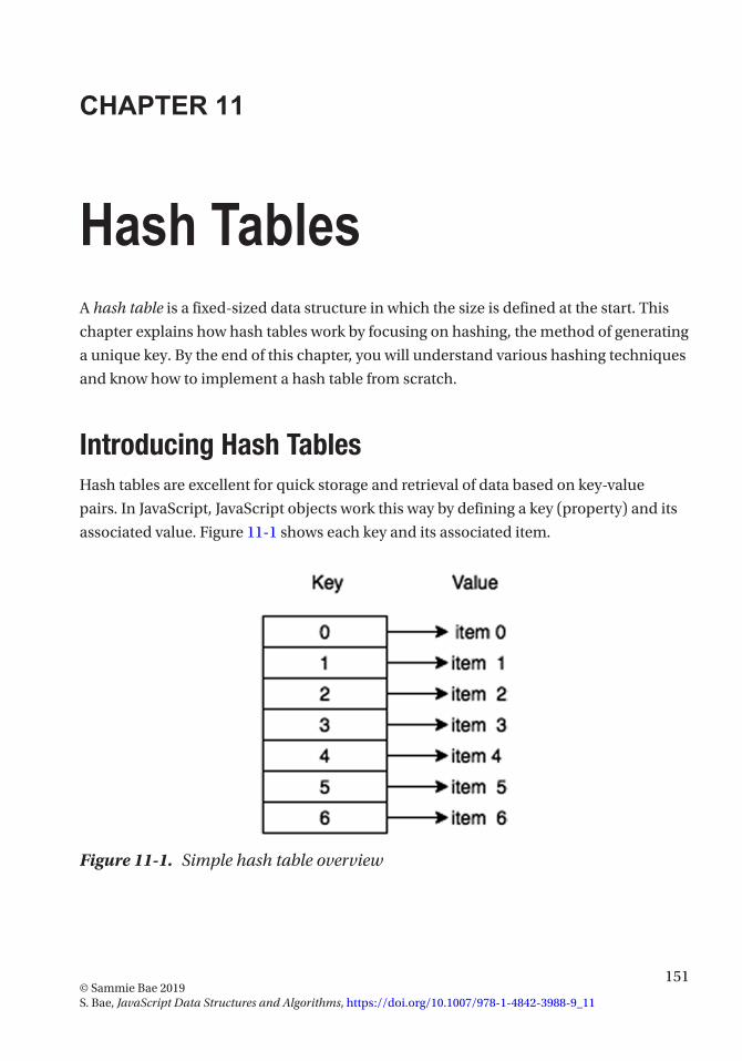
151© Sammie Bae 2019 S. Bae, JavaScript Data Structures and Algorithms, https://doi.org/10.1007/978-1-4842-3988-9_11
CHAPTER 11
Hash TablesA hash table is a fixed-sized data structure in which the size is defined at the start. This
chapter explains how hash tables work by focusing on hashing, the method of generating
a unique key. By the end of this chapter, you will understand various hashing techniques
and know how to implement a hash table from scratch.
Introducing Hash TablesHash tables are excellent for quick storage and retrieval of data based on key-value
pairs. In JavaScript, JavaScript objects work this way by defining a key (property) and its
associated value. Figure 11-1 shows each key and its associated item.
Figure 11-1. Simple hash table overview

152
A hash table contains two main functions: put() and get(). put() is used for storing
data into the hash table, while get() is used for retrieving data from the hash table. Both
of these functions have a time complexity of O(1).
In a nutshell, a hash table is analogous to an array whose index is calculated with a
hashing function to identify a space in memory uniquely.
localStorage is an example of a data structure based on a hash table. It is a native
JavaScript object supported by all major browsers. It lets developers persist data inside
the browser, meaning it can be accessed after a session.
1 localStorage.setItem("testKey","testValue");
2 location = location; // refreshes the page
3
4 //-----------------------------------
5 localStorage.getItem("testKey"); // prints "testValue"
Hashing TechniquesThe most important part of a hash table is the hash function. The hash function converts
a specified key into an index for an array that stores all of the data. The three primary
requirements for a good hash function are as follows:
• Deterministic: Equal keys produce equal hash values.
• Efficiency: It should be O(1) in time.
• Uniform distribution: It makes the most use of the array.
The first technique for hashing is to use prime numbers. By using the modulus
operator with prime numbers, a uniform distribution of the index can be guaranteed.
Prime Number HashingPrime numbers in hashing are important. This is because modulus division using prime
numbers yields an array index in a distributed manner.
Modulus number: 11
4 % 11 = 4
7 % 11 = 7
9 % 11 = 9
15 % 11 = 4
Chapter 11 hash tables

153
Collisions can be seen with 15 and 4 yielding the same key; handling this collision is
discussed later in this chapter. What is important here is that modulus by prime numbers
guarantees the best distribution for a fixed size. Modulus by a small nonprime number
such as 4 guarantees only a range from 0 to 3 and leads to a large number of collisions.
Modulus number: 4
6 % 4 = 2
10 % 4 = 2
This is the first hashing technique that will be observed. Take a look at Figure 11-2,
which is a hash table with two arrays of size 11, and each of the 11 elements is empty.
One array is for the keys, and the other is for values.
Figure 11-2. Hash table of size 11, with all empty elements
In this example, keys are integers, and strings are being stored as keys. Let’s hash the
following key-value pairs:
{key:7, value: "hi"}
{key:24, value: "hello"}
{key:42, value: "sunny"}
{key:34, value: "weather"}
Prime number: 11
7 % 11 = 7
24 % 11 = 2
42 % 11 = 9
34 % 11 = 1
After all the key-value pairs have been inserted, the resulting hash table is shown in
Figure 11-3.
Chapter 11 hash tables
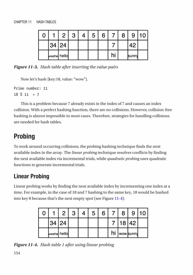
154
Figure 11-3. Hash table after inserting the value pairs
Now let’s hash {key:18, value: “wow”}.
Prime number: 11
18 % 11 = 7
This is a problem because 7 already exists in the index of 7 and causes an index
collision. With a perfect hashing function, there are no collisions. However, collision-free
hashing is almost impossible in most cases. Therefore, strategies for handling collisions
are needed for hash tables.
ProbingTo work around occurring collisions, the probing hashing technique finds the next
available index in the array. The linear probing technique resolves conflicts by finding
the next available index via incremental trials, while quadratic probing uses quadratic
functions to generate incremental trials.
Linear Probing
Linear probing works by finding the next available index by incrementing one index at a
time. For example, in the case of 18 and 7 hashing to the same key, 18 would be hashed
into key 8 because that’s the next empty spot (see Figure 11-4).
Figure 11-4. Hash table 1 after using linear probing
Chapter 11 hash tables

155
However, now when the get(key) function is used, it has to start at the original hash
result (7) and then iterate until 18 is found.
The main disadvantage of linear probing is it easily creates clusters, which are bad
because they create more data to iterate through.
Quadratic Probing
Quadratic probing is a good technique for addressing the cluster issue. Quadratic
probing uses perfect squares instead of incrementing by 1 each time, and this helps to
evenly distribute across the available indices, as shown in Figure 11-5.
h + (1)^2, h + (2)^2, h + (3)^2, h + (4)^2
h + 1, h + 4, h + 9, h + 16
Figure 11-5. Linear probing (on top) and quadratic probing (on bottom)
Rehashing/Double-HashingAnother great way to uniformly distribute the keys is by having a second hashing
function that hashes the result from the original. These are the three primary
requirements for a good second hash function:
• Different: It needs to be different to distribute it better.
• Efficiency: It should still be O(1) in time.
• Nonzero: It should never evaluate to zero. Zero gives the initial
hash value.
A commonly used second hashing function is as follows:
hash2(x) = R − (x % R)
Chapter 11 hash tables

156
Here, x is the result from hashing the first time, and R is less than the size of the
hash table. Each hash collision is resolved by the following, where i is the iteration trial
number:
i * hash2(x)
Hash Table ImplementationNow that hash tables have been explained, let’s implement one from scratch. In this
section, you will apply three different techniques to the same example. The following are
the example key-value pairs that will be used:
7, “hi”
20, “hello”
33, “sunny”
46, “weather”
59, “wow”
72, “forty”
85, “happy”
98, “sad”
Using Linear ProbingLet’s start the example with simple linear probing.
1 function HashTable(size) {
2 this.size = size;
3 this.keys = this.initArray(size);
4 this.values = this.initArray(size);
5 this.limit = 0;
6 }
7
8 HashTable.prototype.put = function(key, value) {
9 if (this.limit >= this.size) throw 'hash table is full'
10
Chapter 11 hash tables

157
11 var hashedIndex = this.hash(key);
12
13 // Linear probing
14 while (this.keys[hashedIndex] != null) {
15 hashedIndex++;
16
17 hashedIndex = hashedIndex % this.size;
18
19 }
20
21 this.keys[hashedIndex] = key;
22 this.values[hashedIndex] = value;
23 this.limit++;
24 }
25
26 HashTable.prototype.get = function(key) {
27 var hashedIndex = this.hash(key);
28
29 while (this.keys[hashedIndex] != key) {
30 hashedIndex++;
31
32 hashedIndex = hashedIndex % this.size;
33
34 }
35 return this.values[hashedIndex];
36 }
37
38 HashTable.prototype.hash = function(key) {
39 // Check if int
40 if (!Number.isInteger(key)) throw 'must be int';
41 return key % this.size;
42 }
43
44 HashTable.prototype.initArray = function(size) {
45 var array = [];
Chapter 11 hash tables

158
46 for (var i = 0; i < size; i++) {
47 array.push(null);
48 }
49 return array;
50 }
51
52 var exampletable = new HashTable(13);
53 exampletable.put(7, "hi");
54 exampletable.put(20, "hello");
55 exampletable.put(33, "sunny");
56 exampletable.put(46, "weather");
57 exampletable.put(59, "wow");
58 exampletable.put(72, "forty");
59 exampletable.put(85, "happy");
60 exampletable.put(98, "sad");
Here is the result:
Keys:
[ 85, 98, null, null, null, null, null, 7, 20, 33, 46, 59, 72 ]
Values:
[ 'happy', 'sad', null, null, null, null, null, 'hi', 'hello',
'sunny', 'weather', 'wow', 'forty' ]
Using Quadratic ProbingNow, let’s change the put() and get() methods to use quadratic probing.
1 HashTable.prototype.put = function (key, value) {
2 if (this.limit >= this.size) throw 'hash table is full'
3
4 var hashedIndex = this.hash(key), squareIndex = 1;
5
6 // quadratic probing
7 while (this.keys[hashedIndex] != null) {
8 hashedIndex += Math.pow(squareIndex,2);
9
Chapter 11 hash tables

159
10 hashedIndex
11 squareIndex++;
12 }
13
14 this.keys[hashedIndex] = key;
15 this.values[hashedIndex] = value;
16 this.limit++;
17 }
18
19 HashTable.prototype.get = function (key) {
20 var hashedIndex = this.hash(key), squareIndex = 1;
21
22 while ( this.keys[hashedIndex] != key ) {
23 hashedIndex += Math.pow(squareIndex, 2);
24
25 hashedIndex = hashedIndex % this.size;
26 squareIndex++;
27 }
28
29 return this.values[hashedIndex];
30 }
Here is the result:
Keys:
[ null, null, null, 85, 72, null, 98, 7, 20, null, 59, 46, 33 ]
Values:
[ null, null, null, 'happy', 'forty', null, 'sad', 'hi', 'hello',
null, 'wow', 'weather', 'sunny' ]
This result is more uniformly distributed than the result from linear probing. It would
be easier to see with a bigger array size and more elements.
Chapter 11 hash tables

160
Using Double-Hashing with Linear ProbingFinally, let’s combine double-hashing and linear probing. Recall the common second
hash function, hash2(x) = R − (x % R), where x is the result from hashing the first time,
and R is less than the size of the hash table.
1 HashTable.prototype.put = function(key, value) {
2 if (this.limit >= this.size) throw 'hash table is full'
3
4 var hashedIndex = this.hash(key);
5
6 while (this.keys[hashedIndex] != null) {
7 hashedIndex++;
8
9 hashedIndex = hashedIndex % this.size;
10
11 }
12 this.keys[hashedIndex] = key;
13 this.values[hashedIndex] = value;
14 this.limit++;
15 }
16
17 HashTable.prototype.get = function(key) {
18 var hashedIndex = this.hash(key);
19
20 while (this.keys[hashedIndex] != key) {
21 hashedIndex++;
22
23 hashedIndex = hashedIndex % this.size;
24
25 }
26 return this.values[hashedIndex];
27 }
28
29 HashTable.prototype.hash = function(key) {
30 if (!Number.isInteger(key)) throw 'must be int'; // check if int
Chapter 11 hash tables

161
31 return this.secondHash(key % this.size);
32 }
33
34 HashTable.prototype.secondHash = function(hashedKey) {
35 var R = this.size - 2;
36 return R - hashedKey % R;
37 }
Here is the result:
Keys:
[ null, 59, 20, 85, 98, 72, null, 7, null, 46, null, 33, null ]
Values:
[ null, 'wow', 'hello', 'happy', 'sad', 'forty', null, 'hi', null,
'weather', null, 'sunny', null ]
Again, double-hashing results in a more uniformly distributed array than the result
from linear probing. Both quadratic probing and double-hashing are great techniques to
reduce the number of collisions in a hash table. There are collision resolution algorithms
far more advanced than these techniques, but they are beyond the scope of this book.
SummaryA hash table is a fixed-sized data structure in which the size is defined at the start.
Hash tables are implemented using a hash function to generate an index for the array.
A good hash function is deterministic, efficient, and uniformly distributive. Hash collisions
should be minimized with a good uniformly distributive hash function, but having some
collisions is unavoidable. Hash collision-handling techniques include but are not limited
to linear probing (incrementing the index by 1), quadratic probing (using a quadratic
function to increment the index), and double-hashing (using multiple hash functions).
The next chapter explores stacks and queues, which are dynamically sized data
structures.
Chapter 11 hash tables

163© Sammie Bae 2019 S. Bae, JavaScript Data Structures and Algorithms, https://doi.org/10.1007/978-1-4842-3988-9_12
CHAPTER 12
Stacks and QueuesThis chapter covers stacks and queues; both are versatile data structures commonly used
in the implementation of other, more complex data structures. You will learn what stacks
and queues are, how and when they are used, and how to implement them. Finally, the
exercises will help you to understand these concepts as well as when to apply stacks and
queues to an algorithmic problem.
StacksA stack is a data structure in which only the last inserted element can be removed
and accessed (see Figure 12-1). Think about stacking plates on a table. To get to the
bottom one, you must remove all the other ones on the top. This is a principle known
as last in, first out (LIFO). A stack is great because it is fast. Since it is known that the
last element is to be removed, the lookup and insertion happen in a constant time of
O(1). Stacks should be used over arrays when you need to work with data in the LIFO
form where the algorithm needs to access only the last-added element. The limitation
of stacks is that they cannot access the non-last-added element directly like arrays can;
in addition, accessing deeper elements requires you to remove the elements from the
data structure.

164
In JavaScript, arrays have methods that define the stack class: pop and push (as
discussed in Chapter 5). With this, a stack can be easily implemented.
Here is some skeleton code to start. You can find the code on GitHub.1
1 function Stack(array){
2 this.array = [];
3 if(array) this.array = array;
4 }
5
6 Stack.prototype.getBuffer = function(){
7 return this.array.slice();
8 }
9
10 Stack.prototype.isEmpty = function(){
11 return this.array.length == 0;
12 }
13
Figure 12-1. Stack, LIFO
1 https://github.com/Apress/js-data-structures-and-algorithms
Chapter 12 StaCkS and QueueS
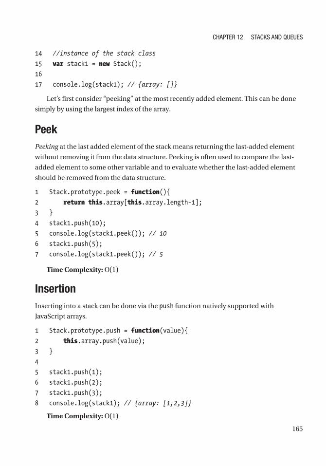
165
14 //instance of the stack class
15 var stack1 = new Stack();
16
17 console.log(stack1); // {array: []}
Let’s first consider “peeking” at the most recently added element. This can be done
simply by using the largest index of the array.
PeekPeeking at the last added element of the stack means returning the last-added element
without removing it from the data structure. Peeking is often used to compare the last-
added element to some other variable and to evaluate whether the last-added element
should be removed from the data structure.
1 Stack.prototype.peek = function(){
2 return this.array[this.array.length-1];
3 }
4 stack1.push(10);
5 console.log(stack1.peek()); // 10
6 stack1.push(5);
7 console.log(stack1.peek()); // 5
Time Complexity: O(1)
InsertionInserting into a stack can be done via the push function natively supported with
JavaScript arrays.
1 Stack.prototype.push = function(value){
2 this.array.push(value);
3 }
4
5 stack1.push(1);
6 stack1.push(2);
7 stack1.push(3);
8 console.log(stack1); // {array: [1,2,3]}
Time Complexity: O(1)
Chapter 12 StaCkS and QueueS

166
DeletionDeletion can also be implemented using a native JavaScript array method, called pop.
1 Stack.prototype.pop = function() {
2 return this.array.pop();
3 };
4
5 stack1.pop(1);
6 stack1.pop(2);
7 stack1.pop(3);
8
9 console.log(stack1); // {array: []}
Time Complexity: O(1)
AccessAccessing specific elements in a data structure is important. Here, let’s take a look at how
to access an element based on order.
To access the nth node from the top, you need to call pop n number of times.
1 function stackAccessNthTopNode(stack, n){
2 var bufferArray = stack.getBuffer();
3 if(n<=0) throw 'error'
4
5 var bufferStack = new Stack(bufferArray);
6
7 while(--n!==0){
8 bufferStack.pop();
9 }
10 return bufferStack.pop();
11 }
12
13 var stack2 = new Stack();
14 stack2.push(1);
Chapter 12 StaCkS and QueueS

167
15 stack2.push(2);
16 stack2.push(3);
17 stackAccessNthTopNode(stack2,2); // 2
Time Complexity: O(n)
Search will be implemented in a similar way.
SearchSearching the stack data structure for a specific element is a critical operation. To do this,
you must first create a buffer stack so that pop can be called on that buffer stack. This
way, the original stack is not mutated, and nothing is removed from it.
1 function stackSearch(stack, element) {
2 var bufferArray = stack.getBuffer();
3
4 var bufferStack = new Stack(bufferArray); // copy into buffer
5
6 while(!bufferStack.isEmpty()){
7 if(bufferStack.pop()==element){
8 return true;
9 }
10 }
11 return false;
12 }
Time Complexity: O(n)
QueuesA queue is also a data structure, but you can remove only the first added element (see
Figure 12-2). This is a principle known as first in, first out (FIFO). A queue is also great
because of the constant time in its operations. Similar to a stack, it has limitations
because only one item can be accessed at a time. Queues should be used over arrays
when you need to work with data in the FIFO form where the algorithm only needs to
access the first added element.
Chapter 12 StaCkS and QueueS

168
In JavaScript, arrays have methods that define the queue class: shift() and push()
(as discussed in Chapter 5). Recall that the shift() method on an array in JavaScript
removes and returns the first element of the array. Adding to a queue is commonly
known as enqueuing, and removing from a queue is known as dequeuing. shift() can be
used for the dequeue, and .push() can be used for the enqueue.
Here is some skeleton code to start. You can find the code on GitHub.2
1 function Queue(array){
2 this.array = [];
3 if(array) this.array = array;
4 }
5
6 Queue.prototype.getBuffer = function(){
7 return this.array.slice();
8 }
9
10 Queue.prototype.isEmpty = function(){
Figure 12-2. Queue, FIFO
2 https://github.com/Apress/js-data-structures-and-algorithms
Chapter 12 StaCkS and QueueS

169
11 return this.array.length == 0;
12 }
13
14 //instance of the queue class
15 var queue1 = new Queue();
16
17 console.log(queue1); // { array: [] }
PeekThe peek function looks at the first item without popping it from the queue. In the stack
implementation, the last element in the array was returned, but a queue returns the first
element in the array because of FIFO.
1 Queue.prototype.peek = function(){
2 return this.array[0];
3 }
InsertionAs mentioned, insertion for a queue is known as enqueue. Since an array is used to hold
the stack data, the push() method can be used to implement enqueue.
1 Queue.prototype.enqueue = function(value){
2 return this.array.push(value);
3 }
Time Complexity: O(1)
DeletionAs mentioned, deletion for a queue also is known as dequeue. Since an array is used
to hold the stack data, the shift() method can be used to remove and return the first
element in the queue.
1 Queue.prototype.dequeue = function() {
2 return this.array.shift();
Chapter 12 StaCkS and QueueS
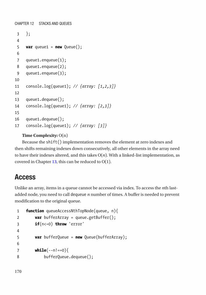
170
3 };
4
5 var queue1 = new Queue();
6
7 queue1.enqueue(1);
8 queue1.enqueue(2);
9 queue1.enqueue(3);
10
11 console.log(queue1); // {array: [1,2,3]}
12
13 queue1.dequeue();
14 console.log(queue1); // {array: [2,3]}
15
16 queue1.dequeue();
17 console.log(queue1); // {array: [3]}
Time Complexity: O(n)
Because the shift() implementation removes the element at zero indexes and
then shifts remaining indexes down consecutively, all other elements in the array need
to have their indexes altered, and this takes O(n). With a linked-list implementation, as
covered in Chapter 13, this can be reduced to O(1).
AccessUnlike an array, items in a queue cannot be accessed via index. To access the nth last-
added node, you need to call dequeue n number of times. A buffer is needed to prevent
modification to the original queue.
1 function queueAccessNthTopNode(queue, n){
2 var bufferArray = queue.getBuffer();
3 if(n<=0) throw 'error'
4
5 var bufferQueue = new Queue(bufferArray);
6
7 while(--n!==0){
8 bufferQueue.dequeue();
Chapter 12 StaCkS and QueueS

171
9 }
10 return bufferQueue.dequeue();
11 }
Time Complexity: O(n)
SearchYou might need to search a queue to check whether an element exists within a queue.
Again, this involves creating a buffer queue first to avoid modifications to the original
queue.
1 function queueSearch(queue, element){
2 var bufferArray = queue.getBuffer();
3
4 var bufferQueue = new Queue(bufferArray);
5
6 while(!bufferQueue.isEmpty()){
7 if(bufferQueue.dequeue()==element){
8 return true;
9 }
10 }
11 return false;
12 }
Time Complexity: O(n)
SummaryBoth stacks and queues support peek, insertion, and deletion in O(1). The most
important distinction between a stack and a queue is that a stack is LIFO and a queue is
FIFO. Table 12-1 summarizes the time complexity.
Chapter 12 StaCkS and QueueS

172
ExercisesAll the code for the exercises can be found on GitHub.4
DESIGN A STACK USING ONLY QUEUES AND THEN DESIGN A QUEUE USING ONLY STACKS
Stack Using Queues
a queue can be made with two stacks. a queue is a data structure that returns the first-added
element with the dequeue() method. a stack is a data structure that returns the last-added
element via pop. In other words, a queue removes elements in the reverse direction of a stack.
For example, examine a stack array with [1,2,3,4,5].
to reverse the order, all of the elements could be pushed onto a second stack and pop that
second stack. So, the second stack array will look like this: [5,4,3,2,1].
When this is popped off, the last element is removed, which is 1. So, 1 is originally the first
element. hence, a queue was implemented using only two stacks.
1 function TwoStackQueue(){
2 this.inbox = new Stack();
3 this.outbox= new Stack();
4 }
5
6 TwoStackQueue.prototype.enqueue = function(val) {
7 this.inbox.push(val);
Table 12-1. Queue and Stack Time Complexity Summary
Access Search Peek Insertion Deletion
Queue O(n) O(n) O(1) O(1) O(n)3
Stack O(n) O(n) O(1) O(1) O(1)
3 This could be improved to O(1) with a linked-list implementation.4 https://github.com/Apress/js-data-structures-and-algorithms
Chapter 12 StaCkS and QueueS

173
8 }
9
10 TwoStackQueue.prototype.dequeue = function() {
11 if(this.outbox.isEmpty()){
12 while(!this.inbox.isEmpty()){
13 this.outbox.push(this.inbox.pop());
14 }
15 }
16 return this.outbox.pop();
17 };
18 var queue = new TwoStackQueue();
19 queue.enqueue(1);
20 queue.enqueue(2);
21 queue.enqueue(3);
22 queue.dequeue(); // 1
23 queue.dequeue(); // 2
24 queue.dequeue(); // 3
Queue Using Stacks
a stack can be made with two queues. a stack is a data structure that returns the last
element. to implement this using a queue, simply enqueue all the elements inside the main
queue except for the last element. then return that last element.
1 function QueueStack(){
2 this.inbox = new Queue(); // first stack
3 }
4
5 QueueStack.prototype.push = function(val) {
6 this.inbox.enqueue(val);
7 };
8
9 QueueStack.prototype.pop = function() {
10 var size = this.inbox.array.length-1;
11 var counter =0;
12 var bufferQueue = new Queue();
13
14 while(++counter<=size){
15 bufferQueue.enqueue(this.inbox.dequeue());
Chapter 12 StaCkS and QueueS

174
16 }
17 var popped = this.inbox.dequeue();
18 this.inbox = bufferQueue;
19 return popped
20 };
21
22 var stack = new QueueStack();
23
24 stack.push(1);
25 stack.push(2);
26 stack.push(3);
27 stack.push(4);
28 stack.push(5);
29
30 console.log(stack.pop()); // 5
31 console.log(stack.pop()); // 4
32 console.log(stack.pop()); // 3
33 console.log(stack.pop()); // 2
34 console.log(stack.pop()); // 1
DESIGN A CASHIER CLASS THAT TAKES IN A CUSTOMER OBJECT AND HANDLES FOOD ORDERING ON A FIRST-COME, FIRST-SERVED BASIS
here are the requirements:
1. the cashier requires a customer name and order item for the order.
2. the customer who was served first is processed first.
here are the required implementations:
• addOrder(customer): enqueues a customer object to be processed by
deliverOrder()
• deliverOrder(): prints the name and order for the next customer to be
processed
Chapter 12 StaCkS and QueueS

175
For this exercise, the Cashier class should enqueue customer class objects with a queue and
dequeue them when finished.
1 function Customer(name, order){
2 this.name = name;
3 this.order = order;
4 }
5
6 function Cashier(){
7 this.customers = new Queue();
8 }
9
10 Cashier.prototype.addOrder = function (customer){
11 this.customers.enqueue(customer);
12 }
13
14 Cashier.prototype.deliverOrder = function(){
15 var finishedCustomer = this.customers.dequeue();
16
17 console.log(finishedCustomer.name+", your "+finishedCustomer.order+"
is ready!");
18 }
19
20 var cashier = new Cashier();
21 var customer1 = new Customer('Jim',"Fries");
22 var customer2 = new Customer('Sammie',"Burger");
23 var customer3 = new Customer('Peter',"Drink");
24
25 cashier.addOrder(customer1);
26 cashier.addOrder(customer2);
27 cashier.addOrder(customer3);
28
29 cashier.deliverOrder(); // Jim, your Fries is ready!
30 cashier.deliverOrder(); // Sammie, your Burger is ready!
31 cashier.deliverOrder(); // Peter, your Drink is ready!
Chapter 12 StaCkS and QueueS
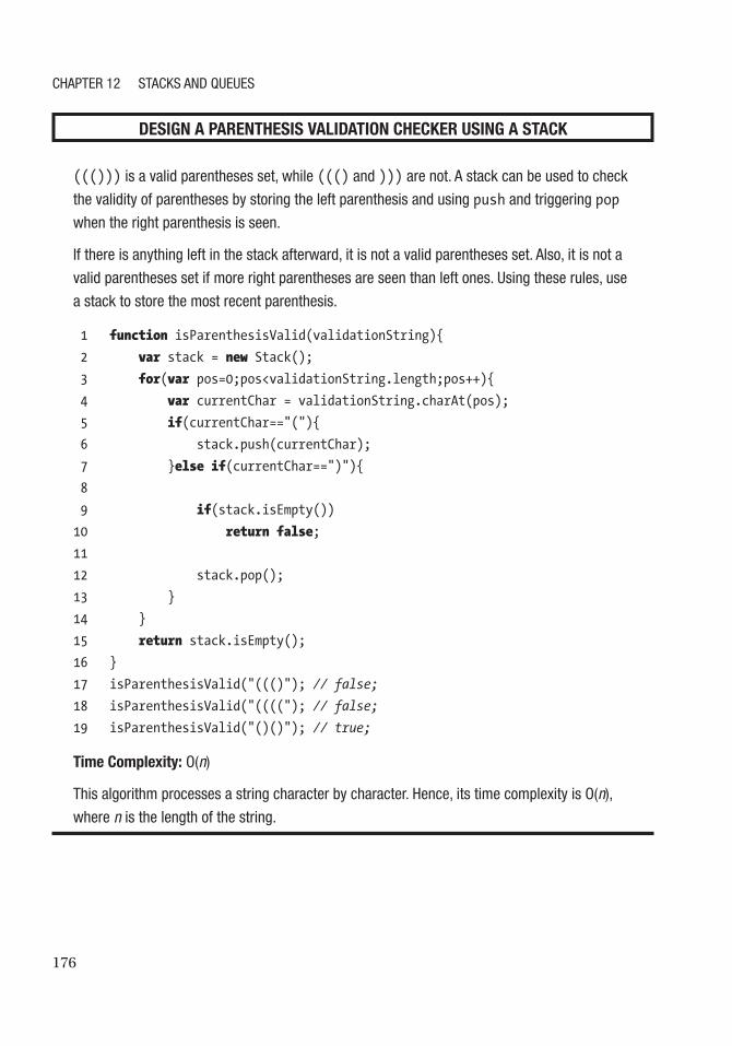
176
DESIGN A PARENTHESIS VALIDATION CHECKER USING A STACK
((())) is a valid parentheses set, while ((() and ))) are not. a stack can be used to check
the validity of parentheses by storing the left parenthesis and using push and triggering pop
when the right parenthesis is seen.
If there is anything left in the stack afterward, it is not a valid parentheses set. also, it is not a
valid parentheses set if more right parentheses are seen than left ones. using these rules, use
a stack to store the most recent parenthesis.
1 function isParenthesisValid(validationString){
2 var stack = new Stack();
3 for(var pos=0;pos<validationString.length;pos++){
4 var currentChar = validationString.charAt(pos);
5 if(currentChar=="("){
6 stack.push(currentChar);
7 }else if(currentChar==")"){
8
9 if(stack.isEmpty())
10 return false;
11
12 stack.pop();
13 }
14 }
15 return stack.isEmpty();
16 }
17 isParenthesisValid("((()"); // false;
18 isParenthesisValid("(((("); // false;
19 isParenthesisValid("()()"); // true;
Time Complexity: O(n)
this algorithm processes a string character by character. hence, its time complexity is O(n),
where n is the length of the string.
Chapter 12 StaCkS and QueueS

177
DESIGN A SORTABLE STACK
the idea is to have two stacks, one that is sorted and one that is nonsorted. When sorting,
pop from the unsorted stack, and when any number smaller (if descending order) or bigger (if
ascending order) on the sorted stack is on top, that sorted stack element should move back to
unsorted because it is out of order. run a loop until the stack is all sorted.
1 function sortableStack(size){
2 this.size = size;
3
4 this.mainStack = new Stack();
5 this.sortedStack = new Stack();
6
7 // let's initialize it with some random ints
8 for(var i=0;i<this.size;i++){
9 this.mainStack.push(Math.floor(Math.random()*11));
10 }
11 }
12
13 sortableStack.prototype.sortStackDescending = function(){
14 while(!this.mainStack.isEmpty()){
15 var temp = this.mainStack.pop();
16 while(!this.sortedStack.isEmpty() && this.sortedStack.peek()< temp){
17 this.mainStack.push(this.sortedStack.pop());
18 }
19 this.sortedStack.push(temp);
20 }
21 }
22
23 var ss = new sortableStack(10);
24 console.log(ss); // [ 8, 3, 4, 4, 1, 2, 0, 9, 7, 8 ]
25 ss.sortStackDescending();
26 console.log(ss.sortedStack); // [ 9, 8, 8, 7, 4, 4, 3, 2, 1, 0 ]
Time Complexity: O(n 2)
this algorithm involves a reshuffling of the elements between two stacks, which in the worst
possible case takes O(n2), where n is the number of elements to be sorted.
Chapter 12 StaCkS and QueueS

179© Sammie Bae 2019 S. Bae, JavaScript Data Structures and Algorithms, https://doi.org/10.1007/978-1-4842-3988-9_13
CHAPTER 13
Linked ListsThis chapter will cover linked lists. A linked list is a data structure in which each node
points to another node. Unlike arrays, which have a fixed size, a linked list is a dynamic
data structure that can allocate and deallocate memory at runtime. By the end of this
chapter, you will understand how to implement and work with linked lists.
There are two types of linked lists discussed in this chapter: singly and doubly linked
lists. Let’s examine the singly linked list first.
Singly Linked ListsThe linked list data structure is one where each node (element) has reference to the next
node (see Figure 13-1).
Figure 13-1. Singly linked list
A node in a singly linked list has the following properties: data and next. data
is the value for the linked list node, and next is a pointer to another instance of
SinglyLinkedListNode.
1 function SinglyLinkedListNode(data) {
2 this.data = data;
3 this.next = null;
4 }

180
The following code is the base for the singly linked list example. You can find the
code on GitHub.1 The code block has a helper function to check whether the singly
linked list is empty.
1 function SinglyLinkedList(){
2 this.head = null;
3 this.size = 0;
4 }
5
6 SinglyLinkedList.prototype.isEmpty = function(){
7 return this.size == 0;
8 }
The start of the linked list is referred to as the head. This property defaults to null
before inserting any element into the linked list.
InsertionThe following code block shows how to insert into a singly linked list. If the head of the
linked list is empty, the head is set to the new node. Otherwise, the old heap is saved in
temp, and the new head becomes the newly added node. Finally, the new head’s next
points to the temp (the old head).
1 SinglyLinkedList.prototype.insert = function(value) {
2 if (this.head === null) { //If first node
3 this.head = new SinglyLinkedListNode(value);
4 } else {
5 var temp = this.head;
6 this.head = new SinglyLinkedListNode(value);
7 this.head.next = temp;
8 }
9 this.size++;
10 }
11 var sll1 = new SinglyLinkedList();
12 sll1.insert(1); // linked list is now: 1 -> null
1 https://github.com/Apress/js-data-structures-and-algorithms
Chapter 13 Linked Lists

181
13 sll1.insert(12); // linked list is now: 12 -> 1 -> null
14 sll1.insert(20); // linked list is now: 20 -> 12 -> 1 -> null
Time Complexity: O(1)
This is a constant time operation; no loops or traversal is required.
Deletion by ValueThe deletion of a node in a singly linked list is implemented by removing the reference of
that node. If the node is in the “middle” of the linked list, this is achieved by having the
node with the next pointer to that node point to that node’s own next node instead, as
shown in Figure 13-2.
Figure 13-2. Interior node removal from a singly linked list
If the node is at the end of the linked list, then the second-to-last element can
dereference the node by setting its next to null.
1 SinglyLinkedList.prototype.remove = function(value) {
2 var currentHead = this.head;
3 if (currentHead.data == value) {
4 // just shift the head over. Head is now this new value
5 this.head = currentHead.next;
6 this.size--;
7 } else {
8 var prev = currentHead;
9 while (currentHead.next) {
10 if (currentHead.data == value) {
Chapter 13 Linked Lists

182
11 // remove by skipping
12 prev.next = currentHead.next;
13 prev = currentHead;
14 currentHead = currentHead.next;
15 break; // break out of the loop
16 }
17 prev = currentHead;
18 currentHead = currentHead.next;
19 }
20 //if wasn't found in the middle or head, must be tail
21 if (currentHead.data == value) {
22 prev.next = null;
23 }
24 this.size--;
25 }
26 }
27 var sll1 = new SinglyLinkedList();
28 sll1.insert(1); // linked list is now: 1 -> null
29 sll1.insert(12); // linked list is now: 12 -> 1 -> null
30 sll1.insert(20); // linked list is now: 20 -> 12 -> 1 -> null
31 sll1.remove(12); // linked list is now: 20 -> 1 -> null
32 sll1.remove(20); // linked list is now: 1 -> null
Time Complexity: O(n)
In the worst case, the entire linked list must be traversed.
Deletion at the HeadDeleting an element at the head of the linked list is possible in O(1). When a node is
deleted from the head, no traversal is required. The implementation of this deletion is
shown in the following code block. This allows the linked list to implement a stack. The
last-added item (to the head) can be removed in O(1).
1 DoublyLinkedList.prototype.deleteAtHead = function() {
2 var toReturn = null;
3
4 if (this.head !== null) {
Chapter 13 Linked Lists
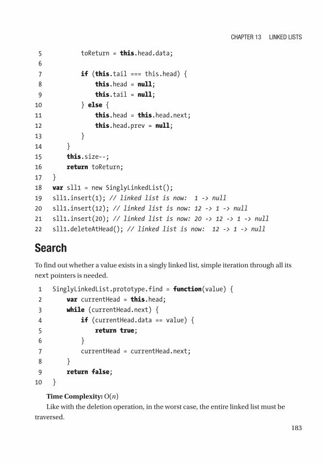
183
5 toReturn = this.head.data;
6
7 if (this.tail === this.head) {
8 this.head = null;
9 this.tail = null;
10 } else {
11 this.head = this.head.next;
12 this.head.prev = null;
13 }
14 }
15 this.size--;
16 return toReturn;
17 }
18 var sll1 = new SinglyLinkedList();
19 sll1.insert(1); // linked list is now: 1 -> null
20 sll1.insert(12); // linked list is now: 12 -> 1 -> null
21 sll1.insert(20); // linked list is now: 20 -> 12 -> 1 -> null
22 sll1.deleteAtHead(); // linked list is now: 12 -> 1 -> null
SearchTo find out whether a value exists in a singly linked list, simple iteration through all its
next pointers is needed.
1 SinglyLinkedList.prototype.find = function(value) {
2 var currentHead = this.head;
3 while (currentHead.next) {
4 if (currentHead.data == value) {
5 return true;
6 }
7 currentHead = currentHead.next;
8 }
9 return false;
10 }
Time Complexity: O(n)
Like with the deletion operation, in the worst case, the entire linked list must be
traversed.
Chapter 13 Linked Lists

184
Doubly Linked ListsA doubly linked list can be thought of as a bidirectional singly linked list. Each node in
the doubly linked list has both a next pointer and a prev pointer. The following code
block implements the doubly linked list node:
1 function DoublyLinkedListNode(data) {
2 this.data = data;
3 this.next = null;
4 this.prev = null;
5 }
In addition, a doubly linked list has a head pointer as well as a tail pointer. The
head refers to the beginning of the doubly linked list, and the tail refers to the end of
the doubly linked list. This is implemented in the following code along with a helper
function to check whether the doubly linked list is empty:
1 function DoublyLinkedList (){
2 this.head = null;
3 this.tail = null;
4 this.size = 0;
5 }
6 DoublyLinkedList.prototype.isEmpty = function(){
7 return this.size == 0;
8 }
Each node in a doubly linked list has next and prev properties. Deletion, insertion,
and search implementations in a doubly linked list are similar to that of the singly linked
list. However, for both insertion and deletion, both next and prev properties must be
updated. Figure 13-3 shows an example of a doubly linked list.
Figure 13-3. Doubly linked list example with five nodes
Chapter 13 Linked Lists

185
Insertion at the HeadInserting into the head of the doubly linked list is the same as the insertion for the singly
linked list except that it has to update the prev pointer as well. The following code block
shows how to insert into the doubly linked list. If the head of the linked list is empty, the
head and the tail are set to the new node. This is because when there is only one element,
that element is both the head and the tail. Otherwise, the temp variable is used to store the
new node. The new node’s next points to the current head, and then the current head’s
prev points to the new node. Finally, the head pointer is updated to the new node.
1 DoublyLinkedList.prototype.addAtFront = function(value) {
2 if (this.head === null) { //If first node
3 this.head = new DoublyLinkedListNode(value);
4 this.tail = this.head;
5 } else {
7 var temp = new DoublyLinkedListNode(value);
8 temp.next = this.head;
9 this.head.prev = temp;
10 this.head = temp;
11 }
12 this.size++;
13 }
14 var dll1 = new DoublyLinkedList();
15 dll1.insertAtHead(10); // ddl1's structure: tail: 10 head: 10
16 dll1.insertAtHead(12); // ddl1's structure: tail: 10 head: 12
17 dll1.insertAtHead(20); // ddl1's structure: tail: 10 head: 20
Time Complexity: O(1)
Insertion at the TailSimilarly, a new node can be added to the tail of a doubly linked list, as implemented in
the following code block:
1 DoublyLinkedList.prototype.insertAtTail = function(value) {
2 if (this.tail === null) { //If first node
3 this.tail = new DoublyLinkedListNode(value);
Chapter 13 Linked Lists

186
4 this.head = this.tail;
5 } else {
6 var temp = new DoublyLinkedListNode(value);
7 temp.prev = this.tail;
8 this.tail.next = temp;
9 this.tail = temp;
10 }
11 this.size++;
12 }
13
14 var dll1 = new DoublyLinkedList();
15 dll1.insertAtHead(10); // ddl1's structure: tail: 10 head: 10
16 dll1.insertAtHead(12); // ddl1's structure: tail: 10 head: 12
17 dll1.insertAtHead(20); // ddl1's structure: tail: 10 head: 20
18 dll1.insertAtTail(30); // ddl1's structure: tail: 30 head: 20
Time Complexity: O(1)
Deletion at the HeadRemoving a node at the head from a doubly linked list can be done in O(1) time. If there
is only one item in the case that the head and the tail are the same, both the head and the
tail are set to null. Otherwise, the head is set to the head’s next pointer. Finally, the new
head’s prev is set to null to remove the reference of the old head. This is implemented
in the following code block. This is great because it can be used like a dequeue function
from the queue data structure.
1 DoublyLinkedList.prototype.deleteAtHead = function() {
2 var toReturn = null;
3
4 if (this.head !== null) {
5 toReturn = this.head.data;
6
7 if (this.tail === this.head) {
8 this.head = null;
9 this.tail = null;
10 } else {
Chapter 13 Linked Lists
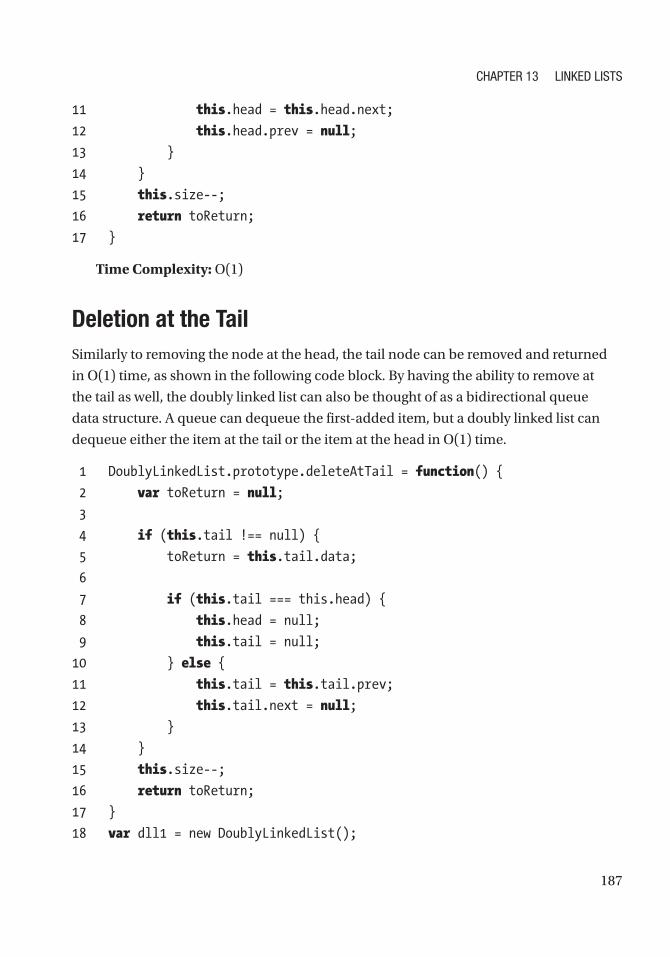
187
11 this.head = this.head.next;
12 this.head.prev = null;
13 }
14 }
15 this.size--;
16 return toReturn;
17 }
Time Complexity: O(1)
Deletion at the TailSimilarly to removing the node at the head, the tail node can be removed and returned
in O(1) time, as shown in the following code block. By having the ability to remove at
the tail as well, the doubly linked list can also be thought of as a bidirectional queue
data structure. A queue can dequeue the first-added item, but a doubly linked list can
dequeue either the item at the tail or the item at the head in O(1) time.
1 DoublyLinkedList.prototype.deleteAtTail = function() {
2 var toReturn = null;
3
4 if (this.tail !== null) {
5 toReturn = this.tail.data;
6
7 if (this.tail === this.head) {
8 this.head = null;
9 this.tail = null;
10 } else {
11 this.tail = this.tail.prev;
12 this.tail.next = null;
13 }
14 }
15 this.size--;
16 return toReturn;
17 }
18 var dll1 = new DoublyLinkedList();
Chapter 13 Linked Lists

188
19 dll1.insertAtHead(10); // ddl1's structure: tail: 10 head: 10
20 dll1.insertAtHead(12); // ddl1's structure: tail: 10 head: 12
21 dll1.insertAtHead(20); // ddl1's structure: tail: 10 head: 20
22 dll1.insertAtTail(30); // ddl1's structure: tail: 30 head: 20
23 dll1.deleteAtTail();
24 // ddl1's structure: tail: 10 head: 20
Time Complexity: O(1)
SearchTo find out whether a value exists in a doubly linked list, you can start at the head and
use the next pointer or start at the tail and use the prev pointer. The following code
block is the same implementation as the singly linked list search implementation, which
starts at the head and looks for the item:
1 DoublyLinkedList.prototype.findStartingHead = function(value) {
2 var currentHead = this.head;
3 while(currentHead.next){
4 if(currentHead.data == value){
5 return true;
6 }
7 currentHead = currentHead.next;
8 }
9 return false;
10 }
11 var dll1 = new DoublyLinkedList();
12 dll1.insertAtHead(10); // ddl1's structure: tail: 10 head: 10
13 dll1.insertAtHead(12); // ddl1's structure: tail: 10 head: 12
14 dll1.insertAtHead(20); // ddl1's structure: tail: 10 head: 20
15 dll1.insertAtTail(30); // ddl1's structure: tail: 30 head: 20
16 dll1.findStartingHead(10); // true
17 dll1.findStartingHead(100); // false
Time Complexity: O(n)
Chapter 13 Linked Lists

189
The following code traverses the doubly linked list starting with the tail using prev
pointers:
1 DoublyLinkedList.prototype.findStartingTail = function(value) {
2 var currentTail = this.tail;
3 while (currentTail.prev){
4 if(currentTail.data == value){
5 return true;
6 }
7 currentTail = currentTail.prev;
8 }
9 return false;
10 }
11
12 var dll1 = new DoublyLinkedList();
13 dll1.insertAtHead(10); // ddl1's structure: tail: 10 head: 10
14 dll1.insertAtHead(12); // ddl1's structure: tail: 10 head: 12
15 dll1.insertAtHead(20); // ddl1's structure: tail: 10 head: 20
16 dll1.insertAtTail(30); // ddl1's structure: tail: 30 head: 20
17 dll1.findStartingTail(10); // true
18 dll1.findStartingTail(100); // false
Time Complexity: O(n)
Although the time complexity for search is the same as the singly linked list’s search,
only the doubly linked list can search bidirectionally (using prev or next). This means
that if given a reference to a doubly linked list node, doubly linked lists can perform a full
search, but a singly linked list is limited to only its next pointers.
SummaryThe linked list data structure works by each node having a next pointer (and previous, or
prev, pointer if doubly linked) to a different node. Insertion for both singly and doubly
linked lists has a constant time complexity of O(1). The time complexity of deleting
from the head of the singly and doubly linked lists is O(1) as well. However, searching
for an item in both singly and doubly linked list takes O(n) time. Doubly linked lists
should be used over singly linked lists when bidirectional traversal/search is required.
Furthermore, doubly linked lists allow you to pop from either the tail or the head of the
linked list for a flexible and fast O(1) operation.
Chapter 13 Linked Lists
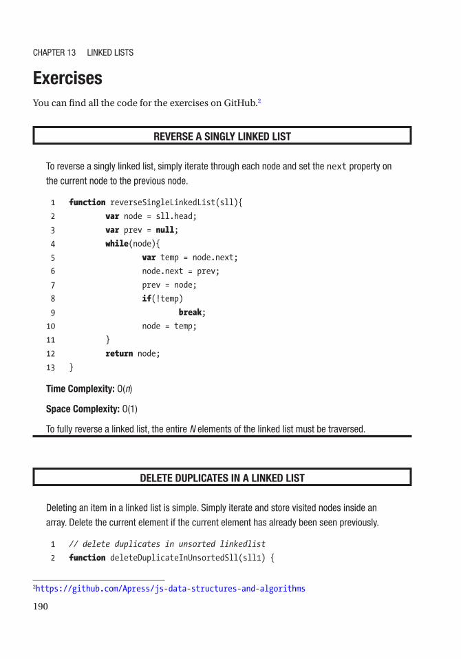
190
ExercisesYou can find all the code for the exercises on GitHub.2
REVERSE A SINGLY LINKED LIST
to reverse a singly linked list, simply iterate through each node and set the next property on
the current node to the previous node.
1 function reverseSingleLinkedList(sll){
2 var node = sll.head;
3 var prev = null;
4 while(node){
5 var temp = node.next;
6 node.next = prev;
7 prev = node;
8 if(!temp)
9 break;
10 node = temp;
11 }
12 return node;
13 }
Time Complexity: O(n)
Space Complexity: O(1)
to fully reverse a linked list, the entire N elements of the linked list must be traversed.
DELETE DUPLICATES IN A LINKED LIST
deleting an item in a linked list is simple. simply iterate and store visited nodes inside an
array. delete the current element if the current element has already been seen previously.
1 // delete duplicates in unsorted linkedlist
2 function deleteDuplicateInUnsortedSll(sll1) {
2 https://github.com/Apress/js-data-structures-and-algorithms
Chapter 13 Linked Lists

191
3 var track = [];
4
5 var temp = sll1.head;
6 var prev = null;
7 while (temp) {
8 if (track.indexOf(temp.data) >= 0) {
9 prev.next = temp.next;
10 sll1.size--;
11 } else {
12 track.push(temp.data);
13 prev = temp;
14 }
15 temp = temp.next;
16 }
17 console.log(temp);
18 }
Time Complexity: O(n2)
Space Complexity: O(n)
however, this algorithm must iterate over the array with the .indexOf() method, which is
O(n) as well as iterating n times. hence, it is O(n2) in time complexity. in addition, the track
array grows to size of N, and this causes the space complexity to be O(n). Let’s cut the time
complexity down to O(n).
1 //delete duplicates in unsorted linkedlist
2 function deleteDuplicateInUnsortedSllBest(sll1) {
3 var track = {};
4
5 var temp = sll1.head;
6 var prev = null;
7 while (temp) {
8 if (track[temp.data]) {
9 prev.next = temp.next;
10 sll1.size--;
11 } else {
12 track[temp.data] = true;
13 prev = temp;
14 }
Chapter 13 Linked Lists

192
15 temp = temp.next;
16 }
17 console.log(temp);
18 }
Time Complexity: O(n)
Space Complexity: O(n)
Use of the Javascript Object as a hash table to store and check for seen elements cuts it
down to O(n) but O(n) in space as extra memory is required for the hash table.
Chapter 13 Linked Lists
193© Sammie Bae 2019 S. Bae, JavaScript Data Structures and Algorithms, https://doi.org/10.1007/978-1-4842-3988-9_14
CHAPTER 14
CachingCaching is the process of storing data into temporary memory so that it can be easily
retrieved for later use if it is required again. As an example, a database system keeps data
cached to avoid rereading the hard drive, and a web browser caches web pages (images
and assets) to avoid redownloading the contents. Put simply, in caching, the goal is to
maximize hits (an item is in the cache when requested) and minimize misses (an item is
not in the cache when requested).
In this chapter, two caching techniques will be discussed: least frequently used (LFU)
and least recently used (LRU) caching.
Note The concept of caching comes from the world of operating systems. You can read more about it in a lecture presentation1 by Jeff Zarnett from the University of Waterloo.
Understanding CachingCache design generally considers these two factors:
• Temporal locality: A memory location that has been recently
accessed is likely to be accessed again.
• Spatial locality: A memory location near one that has recently been
accessed is likely to be accessed again.
1 https://github.com/jzarnett/ece254/blob/master/lectures/L21-slides-Memory_Segmentation_Paging.pdf
194
The optimal caching algorithm would be able to replace the part of the cache that
will be used most distantly in the future with the new element to be inserted. This
will require, for each item, calculating how many time in the future that item will be
accessed. It should be obvious to you that this is impossible to implement because it
requires looking into the future.
Least Frequently Used CachingLeast frequently used (LFU) caching is a caching algorithm used by the operating
system to manage memory. The system tracks the number of times a block is
referenced in memory. By design, when the cache exceeds its limit, the system
deletes the item with the lowest reference frequency. The easiest implementation
of the LFU cache is assigning a counter to every block loaded into the cache and
incrementing a counter every time a reference is made to that block. When the cache
exceeds its limit, the system searches for the block with the lowest counter and
removes it from the cache.
Although LFU caching seems like an intuitive approach, it is not ideal when an item
in memory is referenced repeatedly for a short amount of time and not accessed again.
The frequency for that block is high because of its repeated reference, but this forces the
system to delete other blocks that may be used more frequently outside the short block
of time. In addition, new items in the system are susceptible to being deleted quickly
because of their lower frequency of being accessed. Because of these issues, LFU is
uncommon, but some hybrid systems utilize the core LFU concept. Examples of a such
system are mobile keyboard apps. Suggested words appear on the keyboard apps, and
it makes sense to implement this using LFU caching since the user likely uses the same
words often. The frequency of a word would a great metric to see whether the word
should exist in the cache.
The LFU cache uses a doubly linked list to remove elements in O(1) time. The doubly
linked node in LFUs also has the freqCount property, which represents how frequently it
has been accessed/set after being inserted for the first time.
1 function LFUNode(key, value) {
2 this.prev = null;
3 this.next = null;
4 this.key = key;
ChapTer 14 CaChing

195
5 this.data = value;
6 this.freqCount = 1;
7 }
The LFU cache has two hash tables: keys and freq. freq has keys of frequency
(1 to n, where n is the top frequency for element access), and each item is an instance of
a doubly linked list class. keys stores each doubly linked list node for O(1) retrieval. The
classes for a doubly linked list and the LFU cache are defined here:
1 function LFUDoublyLinkedList(){
2 this.head = new LFUNode('buffer head',null);
3 this.tail = new LFUNode('buffer tail',null);
4 this.head.next = this.tail;
5 this.tail.prev = this.head;
6 this.size = 0;
7 }
8
9 function LFUCache(capacity){
10 this.keys = {}; // stores LFUNode
11 this.freq = {}; // stores LFUDoublyLinkedList
12 this.capacity = capacity;
13 this.minFreq = 0;
14 this.size =0;
15 }
The LFUDoublyLinkedList class also requires the doubly linked list implementation
for insertion and removal. However, only the insertion at the head and the removal at the
tail is needed. This implementation is the same as the implementation from the doubly
linked list class shown in Chapter 13 (Linked Lists).
1 LFUDoublyLinkedList.prototype.insertAtHead = function(node) {
2 node.next = this.head.next;
3 this.head.next.prev = node;
4 this.head.next = node;
5 node.prev = this.head;
6 this.size++;
7 }
8
ChapTer 14 CaChing

196
9 LFUDoublyLinkedList.prototype.removeAtTail = function() {
10 var oldTail = this.tail.prev;
11 var prev = this.tail.prev;
12 prev.prev.next = this.tail;
13 this.tail.prev = prev.prev;
14 this.size--;
15 return oldTail;
16 }
17
18 LFUDoublyLinkedList.prototype.removeNode = function(node) {
19 node.prev.next = node.next
20 node.next.prev = node.prev
21 this.size--;
22 }
Implementing set for the LFU has a few steps. There are two cases: insert the new
item and replace an old item. When inserting a new item, a new node is created. If the
cache is not full, it can be inserted into the freq’s doubly linked list of frequency 1. If the
capacity is full, the tail item in the doubly linked list of frequency is deleted, and then the
new node is inserted.
If the element already exists and needs to be replaced, the node is brought to the
head of its corresponding frequency doubly linked list. Finally, the minimum frequency
variable, minFreq, is incremented accordingly to compute which item should be evicted
in the future.
1 LFUCache.prototype.set = function(key, value) {
2 var node = this.keys[key];
3
4 if (node == undefined) {
5 node = new LFUNode(key, value);
6
7 this.keys[key] = node;
8
9 if (this.size != this.capacity) {
10 // insert without deleting
11 if (this.freq[1] === undefined){
ChapTer 14 CaChing
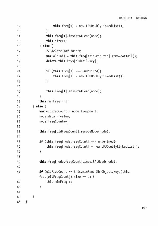
197
12 this.freq[1] = new LFUDoublyLinkedList();
13 }
14 this.freq[1].insertAtHead(node);
15 this.size++;
16 } else {
17 // delete and insert
18 var oldTail = this.freq[this.minFreq].removeAtTail();
19 delete this.keys[oldTail.key];
20
21 if (this.freq[1] === undefined){
22 this.freq[1] = new LFUDoublyLinkedList();
23 }
24
25 this.freq[1].insertAtHead(node);
26 }
27 this.minFreq = 1;
28 } else {
29 var oldFreqCount = node.freqCount;
30 node.data = value;
31 node.freqCount++;
32
33 this.freq[oldFreqCount].removeNode(node);
34
35 if (this.freq[node.freqCount] === undefined){
36 this.freq[node.freqCount] = new LFUDoublyLinkedList();
37 }
38
39 this.freq[node.freqCount].insertAtHead(node);
40
41 if (oldFreqCount == this.minFreq && Object.keys(this.
freq[oldFreqCount]).size == 0) {
42 this.minFreq++;
43 }
44
45 }
46 }
ChapTer 14 CaChing

198
To implement get, the cache needs to return existing nodes in O(1) time and
increment the counter for accessing. If the element does not exist in the cache, it is
forced to return a null element. Otherwise, the frequency for the element is increased,
the item is brought to the head of the doubly linked list, and the minimum frequency
variable, minFreq, is adjusted accordingly.
1 LFUCache.prototype.get = function(key) {
2 var node = this.keys[key];
3
4 if (node == undefined) {
5 return null;
6 } else {
7
8 var oldFreqCount = node.freqCount;
9 node.freqCount++;
10
11 this.freq[oldFreqCount].removeNode(node);
12
13 if (this.freq[node.freqCount] === undefined){
14 this.freq[node.freqCount] = new LFUDoublyLinkedList();
15 }
16
17 this.freq[node.freqCount].insertAtHead(node);
18
19 if (oldFreqCount == this.minFreq && Object.keys(this.
freq[oldFreqCount]).length == 0) {
20 this.minFreq++;
21 }
22 return node.data;
23 }
24 }
ChapTer 14 CaChing

199
With all the functions defined, the following code shows an example of this LFU
usage:
1 var myLFU = new LFUCache(5);
2 myLFU.set(1, 1); // state of myLFU.freq: {1: 1}
3 myLFU.set(2, 2); // state of myLFU.freq: {1: 2<->1}
4 myLFU.set(3, 3); // state of myLFU.freq: {1: 3<->2<->1}
5 myLFU.set(4, 4); // state of myLFU.freq: {1: 4<->3<->2<->1}
6 myLFU.set(5, 5); // state of myLFU.freq: {1: 5<->4<->3<->2<->1}
7 myLFU.get(1); // returns 1, state of myLFU.freq: {1: 5<->4<->3<->2, 2: 1}
8 myLFU.get(1); // returns 1, state of myLFU.freq: {1: 5<->4<->3<->2, 3: 1}
9 myLFU.get(1); // returns 1, state of myLFU.freq: {1: 5<->4<->3<->2, 4: 1}
10 myLFU.set(6, 6); // state of myLFU.freq: {1: 6<->5<->4<->3, 4: 1}
11 myLFU.get(6); // state of myLFU.freq: {1: 5<->4<->3, 4: 1, 2: 6}
Least Recently Used CachingLeast recently used (LRU) caching is a caching algorithm that removes the oldest (least
recently used) items first, so the item replaced is the oldest accessed item. When an item
in the cache is accessed, that item moves to the back (newest in the order) of the list.
When a page not found in the cache is accessed, the front item (or oldest in the order) is
removed, and the new item is put at the back (newest in the order) of the list.
The implementation of this algorithm requires keeping track of which node was used
when. To accomplish this, the LRU cache is implemented using a doubly linked list and
hash table.
A doubly linked list is needed to keep track of the head (the oldest data). A doubly
linked list is required because of the most recently used requirement. Each time new
data is inserted, the head moves up until the size is exceeded. Then the oldest data is
evicted.
Figure 14-1 shows a diagram of an LRU cache with a size of 5.
ChapTer 14 CaChing

200
To implement the LRU cache, the node is defined similarly to the doubly linked list
node in Chapter 13. This node also has a key property, and its implementation is shown
in the following code block:
1 function DLLNode(key, data) {
2 this.key = key;
3 this.data = data;
4 this.next = null;
5 this.prev = null;
6 }
The LRU cache can be initialized by passing the capacity parameter. capacity
defines how many nodes are allowed to be in the cache.
1 function LRUCache(capacity) {
2 this.keys = {};
3 this.capacity = capacity;
4 this.head = new DLLNode(", null);
5 this.tail = new DLLNode(", null);
6 this.head.next = this.tail;
7 this.tail.prev = this.head;
8 }
Figure 14-1. LRU cache
ChapTer 14 CaChing

201
Since the LRU cache uses a doubly linked list, two functions for removing a node and
adding a node to the tail will be defined here:
1 LRUCache.prototype.removeNode = function(node) {
2 var prev = node.prev,
3 next = node.next;
4 prev.next = next;
5 next.prev = prev;
6 }
7
8 LRUCache.prototype.addNode = function(node) {
9 var realTail = this.tail.prev;
10 realTail.next = node;
11
12 this.tail.prev = node;
13 node.prev = realTail;
14 node.next = this.tail;
15 }
Two more functions need to be defined: get and set. Whenever get is called, the
LRU caching scheme brings that node to the head of the doubly linked list since it was
the most recently used node. This is the same as deleting and adding the node. For
setting nodes via set, the keys property on the LRU cache is used to store the node to
keep retrieval in O(1) time in get. However, if the cache is at full capacity, it evicts the
farthest node from the tail.
1 LRUCache.prototype.get = function(key) {
2 var node = this.keys[key];
3 if (node == undefined) {
4 return null;
5 } else {
6 this.removeNode(node);
7 this.addNode(node);
8 return node.data;
9 }
10 }
11
ChapTer 14 CaChing

202
12 LRUCache.prototype.set = function(key, value) {
13 var node = this.keys[key];
14 if (node) {
15 this.removeNode(node);
16 }
17
18 var newNode = new DLLNode(key, value);
19
20 this.addNode(newNode);
21 this.keys[key] = newNode;
22
23 // evict a node
24 if (Object.keys(this.keys).length > this.capacity) {
25 var realHead = this.head.next;
26 this.removeNode(realHead);
27 delete this.keys[realHead.key];
28 }
29 }
Finally, the following is an example of an LRU cache of size 5:
1 var myLRU = new LRUCache(5);
2
3 myLRU.set(1, 1); // 1
4 myLRU.set(2, 2); // 1 <-> 2
5 myLRU.set(3, 3); // 1 <-> 2 <-> 3
6 myLRU.set(4, 4); // 1 <-> 2 <-> 3 <-> 4
7 myLRU.set(5, 5); // 1 <-> 2 <-> 3 <-> 4 <-> 5
8
9
10 myLRU.get(1); // 2 <-> 3 <-> 4 <-> 5 <-> 1
11 myLRU.get(2); // 3 <-> 4 <-> 5 <-> 1 <-> 2
12
13 myLRU.set(6, 6);// 4 <-> 5 <-> 1 <-> 2 <-> 6
14 myLRU.set(7, 7);// 5 <-> 1 <-> 2 <-> 6 <-> 7
15 myLRU.set(8, 8);// 1 <-> 2 <-> 6 <-> 7 <-> 8
ChapTer 14 CaChing

203
SummaryThis chapter covered two main caching ideas: least frequently used and least recently
used. The chapter talked about the concept of an optimal caching algorithm, which is
impossible to implement but provides an idea of what you would want to approximate.
LFU caching sounds great because it uses frequency to determine what node should
be evicted, but LFU is inferior to the LRU in most cases because it does not account for
temporal locality. There are other caching algorithms, but most of those algorithms are
worse in general cases, such as the not recently used and first in, first out algorithms.
Finally, it should be noted that given the many known data of real-life system behavior
workloads, LRU is the most effective algorithm in most cases. Table 14-1 summarizes the
caching algorithms.
Table 14-1. Caching Summary
Algorithm Comment
Optimal impossible to implement
Least frequently used Bad for temporal locality
Least recently used Uses doubly-linked + hashmap
ChapTer 14 CaChing
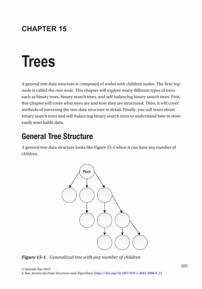
205© Sammie Bae 2019 S. Bae, JavaScript Data Structures and Algorithms, https://doi.org/10.1007/978-1-4842-3988-9_15
CHAPTER 15
TreesA general tree data structure is composed of nodes with children nodes. The first/top
node is called the root node. This chapter will explore many different types of trees
such as binary trees, binary search trees, and self-balancing binary search trees. First,
this chapter will cover what trees are and how they are structured. Then, it will cover
methods of traversing the tree data structure in detail. Finally, you will learn about
binary search trees and self-balancing binary search trees to understand how to store
easily searchable data.
General Tree StructureA general tree data structure looks like Figure 15-1 when it can have any number of
children.
Figure 15-1. Generalized tree with any number of children

206
The code block for the node in the Figure 15-1 tree is as follows:
1 function TreeNode(value){
2 this.value = value;
3 this.children = [];
4 }
Binary TreesA binary tree is a type of tree that has only two children nodes: left and right. See the
following code and Figure 15-2:
1 function BinaryTreeNode(value) {
2 this.value = value;
3 this.left = null;
4 this.right = null;
5 }
Figure 15-2. Binary tree
A binary tree always has a root node (the node at the top), which is initialized to null
before any element is inserted.
1 function BinaryTree(){
2 this._root = null;
3 }
Chapter 15 trees

207
Tree TraversalTraversal through an array is simple: you access the tree using the index and increment
the index until the index reaches the size limit. With trees, the left and right pointers have
to be followed in order to go through every element in the tree. There are various ways to
do this, of course; the most popular traversal techniques are pre-order traversal, post-
order traversal, in-order traversal, and level-order traversal.
All the code for tree traversals is available on GitHub.1
Pre-order TraversalPre-order traversal visits nodes in the following order: root (the current node), left,
right. In Figure 15-3, you can see that 42 is the root, so it’s visited first. Then it goes
left; at this point, the left of the parent (41) is now considered the new root. This new
root (41) is printed; then it goes left again to 10. So, 10 is set to the new root but cannot
continue without a child. Then 40 is visited because that is the right of the previous
parent (41). This process continues, and the whole order is denoted by the gray
squares in Figure 15- 3.
1 https://github.com/Apress/js-data-structures-and-algorithms
Figure 15-3. Pre-order traversal
Chapter 15 trees

208
Recursively, this is implemented easily. The base case terminates when the node is
null. Otherwise, it prints the node value and then calls the recursive function on its left
child and then its right child.
1 BinaryTree.prototype.traversePreOrder = function() {
2 traversePreOrderHelper(this._root);
3
4 function traversePreOrderHelper(node) {
5 if (!node)
6 return;
7 console.log(node.value);
8 traversePreOrderHelper(node.left);
9 traversePreOrderHelper(node.right);
10 }
11 }
This can also be done iteratively, but it is harder to implement.
1 BinaryTree.prototype.traversePreOrderIterative = function() {
2 //create an empty stack and push root to it
3 var nodeStack = [];
4 nodeStack.push(this._root);
5
6 // Pop all items one by one. Do following for every popped item
7 // a) print it
8 // b) push its right child
9 // c) push its left child
10 // Note that right child is pushed first so that left
11 // is processed first */
12 while (nodeStack.length) {
13 //# Pop the top item from stack and print it
14 var node = nodeStack.pop();
15 console.log(node.value);
16
17 //# Push right and left children of the popped node to stack
Chapter 15 trees
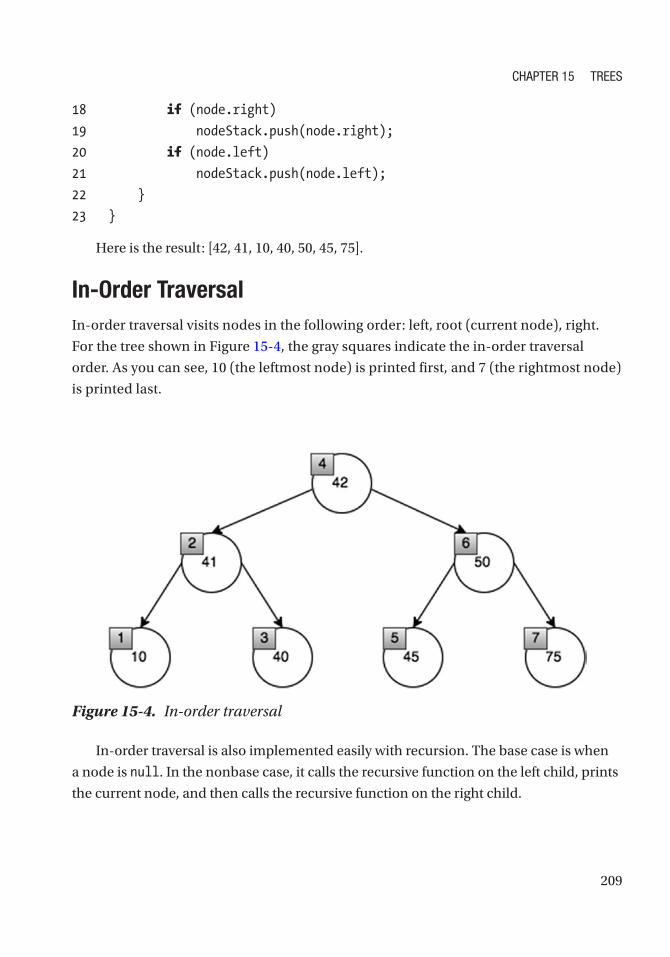
209
18 if (node.right)
19 nodeStack.push(node.right);
20 if (node.left)
21 nodeStack.push(node.left);
22 }
23 }
Here is the result: [42, 41, 10, 40, 50, 45, 75].
In-Order TraversalIn-order traversal visits nodes in the following order: left, root (current node), right.
For the tree shown in Figure 15-4, the gray squares indicate the in-order traversal
order. As you can see, 10 (the leftmost node) is printed first, and 7 (the rightmost node)
is printed last.
Figure 15-4. In-order traversal
In-order traversal is also implemented easily with recursion. The base case is when
a node is null. In the nonbase case, it calls the recursive function on the left child, prints
the current node, and then calls the recursive function on the right child.
Chapter 15 trees
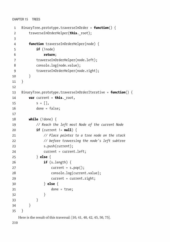
210
1 BinaryTree.prototype.traverseInOrder = function() {
2 traverseInOrderHelper(this._root);
3
4 function traverseInOrderHelper(node) {
5 if (!node)
6 return;
7 traverseInOrderHelper(node.left);
8 console.log(node.value);
9 traverseInOrderHelper(node.right);
10 }
11 }
12
13 BinaryTree.prototype.traverseInOrderIterative = function() {
14 var current = this._root,
15 s = [],
16 done = false;
17
18 while (!done) {
19 // Reach the left most Node of the current Node
20 if (current != null) {
21 // Place pointer to a tree node on the stack
22 // before traversing the node's left subtree
23 s.push(current);
24 current = current.left;
25 } else {
26 if (s.length) {
27 current = s.pop();
28 console.log(current.value);
29 current = current.right;
30 } else {
31 done = true;
32 }
33 }
34 }
35 }
Here is the result of this traversal: [10, 41, 40, 42, 45, 50, 75].
Chapter 15 trees

211
Post-order TraversalPost-order traversal visits nodes in the following order: left, right, root (the current
node). For the tree shown in Figure 15-5, the gray squares indicate the in-order
traversal order. As you can see, 10 (the leftmost node) is printed first, and 42 (the root
node) is printed last.
Figure 15-5. Post-order traversal
Here’s the code:
1 BinaryTree.prototype.traversePostOrder = function() {
2 traversePostOrderHelper(this._root);
3
4 function traversePostOrderHelper(node) {
5 if (node.left)
6 traversePostOrderHelper(node.left);
7 if (node.right)
8 traversePostOrderHelper(node.right);
9 console.log(node.value);
10 }
11 }
12
Chapter 15 trees

212
13 BinaryTree.prototype.traversePostOrderIterative = function() {
14 // Create two stacks
15 var s1 = [],
16 s2 = [];
17
18 // Push root to first stack
19 s1.push(this._root);
20
21 //# Run while first stack is not empty
22 while (s1.length) {
23 // Pop an item from s1 and append it to s2
24 var node = s1.pop();
25 s2.push(node);
26
27 // Push left and right children of removed item to s1
28 if (node.left)
29 s1.push(node.left);
30 if (node.right)
31 s1.push(node.right);
32 }
33 // Print all elements of second stack
34 while (s2.length) {
35 var node = s2.pop();
36 console.log(node.value);
37 }
38 }
Here is the result: [10, 40, 41, 45, 75, 50, 42].
Level-Order TraversalLevel-order traversal, illustrated in Figure 15-6, is also known as breadth first search (BFS).
Chapter 15 trees

213
Figure 15-6. Level-order traversal
More of this will be covered in Chapter 17, but this method essentially visits each
node level by level instead of going deep into the left or right.
1 BinaryTree.prototype.traverseLevelOrder = function() {
2 // Breath first search
3 var root = this._root,
4 queue = [];
5
6 if (!root)
7 return;
8 queue.push(root);
9
10 while (queue.length) {
11 var temp = queue.shift();
12 console.log(temp.value);
13 if (temp.left)
14 queue.push(temp.left);
15 if (temp.right)
16 queue.push(temp.right);
17 }
18 }
Here is the result: [42, 41, 50, 10, 40, 45, 75].
Chapter 15 trees

214
Tree Traversal SummaryIf you know you need to explore the roots before inspecting any leaves, choose pre-order
traversal because you will encounter all the roots before all of the leaves.
If you know you need to explore all the leaves before any nodes, choose post-order
traversal because you don’t waste any time inspecting roots when searching for leaves.
If you know that the tree has an inherent sequence in the nodes and you want to
flatten the tree into its original sequence, then you should use an in-order traversal.
The tree would be flattened in the same way it was created. A pre-order or post-order
traversal might not unwind the tree back into the sequence that was used to create it.
Time Complexity: O(n)
The time complexity of any of these traversals is the same because each traversal
requires that all nodes are visited.
Binary Search TreesBinary search trees (BSTs) also have two children, left and right. However, in a binary
search tree, the left child is smaller than the parent, and the right child is bigger than the
parent. BSTs have this structure because this property enables for searching, inserting,
and removing specific values with O(log2(n)) time complexity.
Figure 15-7 shows the BST property. 1 is smaller than 2, so it is the left child of 2, and
since 3 is bigger than 3, it is the right child of 2.
Figure 15-7. Binary search tree
Chapter 15 trees

215
Binary search trees have a root node (the topmost node), which is originally
initialized null (before any item is inserted).
1 function BinarySearchTree(){
2 this._root = null;
3 }
Figure 15-7 also shows a balanced binary search tree where the height is minimized
by having children on both the left and right sides. However, Figure 15-8 shows an
unbalanced tree where children are only to the right of the parent. This has significant
impact on the data structure and increases the time complexity of insertion, deletion,
and search from O(log2(n)) to O(n). The height of a perfect balanced tree is log2(n), while
an unbalanced tree can be n in the worst case.
Chapter 15 trees

216
InsertionInserting into the BST requires a couple of steps. First, if the root is empty, the root
becomes the new node. Otherwise, a while loop is used to traverse the BST until the
right condition is met. At each loop iteration, it is checked whether the new node is
greater or smaller than the currentRoot.
Figure 15-8. Unbalanced binary search tree
Chapter 15 trees
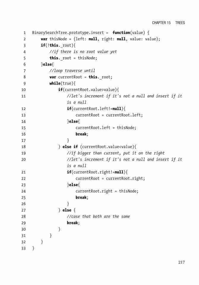
217
1 BinarySearchTree.prototype.insert = function(value) {
2 var thisNode = {left: null, right: null, value: value};
3 if(!this._root){
4 //if there is no root value yet
5 this._root = thisNode;
6 }else{
7 //loop traverse until
8 var currentRoot = this._root;
9 while(true){
10 if(currentRoot.value>value){
11 //let's increment if it's not a null and insert if it
is a null
12 if(currentRoot.left!=null){
13 currentRoot = currentRoot.left;
14 }else{
15 currentRoot.left = thisNode;
16 break;
17 }
18 } else if (currentRoot.value<value){
19 //if bigger than current, put it on the right
20 //let's increment if it's not a null and insert if it
is a null
21 if(currentRoot.right!=null){
22 currentRoot = currentRoot.right;
23 }else{
24 currentRoot.right = thisNode;
25 break;
26 }
27 } else {
28 //case that both are the same
29 break;
30 }
31 }
32 }
33 }
Chapter 15 trees

218
Time Complexity (for balanced trees): O(log2(n))
Time Complexity (for unbalanced trees): O(n)
Time complexity is dependent on the height of the binary search tree.
DeletionThis algorithm works by first traversing down the tree looking specifically for the node
with the specified value. When the node is found, there are three possible cases:
• Case 1: The node has no children.
This is the simplest case. If the node has no child, return null.
That node has been deleted now.
• Case 2: The node has one child.
If the node has one child, simply return the existing child. That
child has now bubbled up and replaced the parent.
• Case 3: The node has two children.
If the node has two children, either find the maximum of the left
subtree or find the minimum of the right subtree to replace that
node.
The following code implements the described three cases. First, it traverses
recursively until one of those cases is met, and then the node is removed.
1 BinarySearchTree.prototype.remove = function(value) {
2
3 return deleteRecursively(this._root, value);
4
5 function deleteRecursively(root, value) {
6 if (!root) {
7 return null;
8 } else if (value < root.value) {
9 root.left = deleteRecursively(root.left, value);
10 } else if (value > root.value) {
11 root.right = deleteRecursively(root.right, value);
Chapter 15 trees

219
12 } else {
13 //no child
14 if (!root.left && !root.right) {
15 return null; // case 1
16 } else if (!root.left) { // case 2
17 root = root.right;
18 return root;
19 } else if (!root.right) { // case 2
20 root = root.left;
21 return root;
22 } else {
23 var temp = findMin(root.right); // case 3
24 root.value = temp.value;
25 root.right = deleteRecursively(root.right, temp.
value);
26 return root;
27 }
28 }
29 return root;
30 }
31
32 function findMin(root) {
33 while (root.left) {
34 root = root.left;
35 }
36 return root;
37 }
38 }
Time Complexity (for balanced tree): O(log2(n))
Time Complexity (for unbalanced trees): O(n)
Time complexity for deletion is also O(log2(n)) because at most that’s the height that
will need to be traversed to find and delete the desired node.
Chapter 15 trees

220
SearchSearch can be performed using the property that BST node’s left child is always
smaller than its parent and that BST node’s right child is always greater than its parent.
Traversing the tree can be done by checking whether currentRoot is smaller or greater
than the value to be searched. If currentRoot is smaller, the right child is visited. If
currentRoot is bigger, the left child is visited.
1 BinarySearchTree.prototype.findNode = function(value) {
2 var currentRoot = this._root,
3 found = false;
4 while (currentRoot) {
5 if (currentRoot.value > value) {
6 currentRoot = currentRoot.left;
7 } else if (currentRoot.value < value) {
8 currentRoot = currentRoot.right;
9 } else {
10 //we've found the node
11 found = true;
12 break;
13 }
14 }
15 return found;
16 }
17 var bst1 = new BinarySearchTree();
18 bst1.insert(1);
19 bst1.insert(3);
20 bst1.insert(2);
21 bst1.findNode(3); // true
22 bst1.findNode(5); // false
Time Complexity (for balanced tree): O(log2(n))
Time Complexity (for unbalanced trees): O(n)
Note that all of the operations’ time complexities are equal to the height of the binary
tree search. With unbalanced binary search trees, the time complexity is high. To address
this, there are families of binary search trees that ensure the height is balanced. One
example of such self-balancing trees is an AVL tree.
Chapter 15 trees
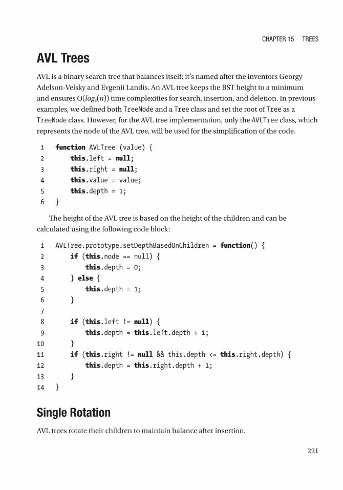
221
AVL TreesAVL is a binary search tree that balances itself; it’s named after the inventors Georgy
Adelson-Velsky and Evgenii Landis. An AVL tree keeps the BST height to a minimum
and ensures O(log2(n)) time complexities for search, insertion, and deletion. In previous
examples, we defined both TreeNode and a Tree class and set the root of Tree as a
TreeNode class. However, for the AVL tree implementation, only the AVLTree class, which
represents the node of the AVL tree, will be used for the simplification of the code.
1 function AVLTree (value) {
2 this.left = null;
3 this.right = null;
4 this.value = value;
5 this.depth = 1;
6 }
The height of the AVL tree is based on the height of the children and can be
calculated using the following code block:
1 AVLTree.prototype.setDepthBasedOnChildren = function() {
2 if (this.node == null) {
3 this.depth = 0;
4 } else {
5 this.depth = 1;
6 }
7
8 if (this.left != null) {
9 this.depth = this.left.depth + 1;
10 }
11 if (this.right != null && this.depth <= this.right.depth) {
12 this.depth = this.right.depth + 1;
13 }
14 }
Single RotationAVL trees rotate their children to maintain balance after insertion.
Chapter 15 trees
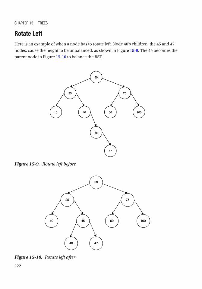
222
Rotate Left
Here is an example of when a node has to rotate left. Node 40’s children, the 45 and 47
nodes, cause the height to be unbalanced, as shown in Figure 15-9. The 45 becomes the
parent node in Figure 15-10 to balance the BST.
Figure 15-10. Rotate left after
Figure 15-9. Rotate left before
Chapter 15 trees

223
To perform a left rotation, first get the left child and store it. This is the “original” left
child. The original left child is to be the parent of the node now. Set the node’s left child
to be the original left child’s left child. Finally, set the right child of the original left child
to be the node.
1 AVLTree.prototype.rotateLL = function() {
2
3 var valueBefore = this.value;
4 var rightBefore = this.right;
5 this.value = this.left.value;
6
7 this.right = this.left;
8 this.left = this.left.left;
9 this.right.left = this.right.right;
10 this.right.right = rightBefore;
11 this.right.value = valueBefore;
12
13 this.right.getDepthFromChildren();
14 this.getDepthFromChildren();
15 };
Rotate Right
Here is an example of when a node has to rotate right. 60’s children, the 55 and 52 nodes,
cause the height to be unbalanced, as shown in Figure 15-11. The 55 node becomes the
parent in Figure 15-12 to balance the BST.
Chapter 15 trees

224
Figure 15-12. Rotate right after
Figure 15-11. Rotate right before
Chapter 15 trees

225
To implement this previously described algorithm, first get the left child and store it.
This the original left child. The original left child is to be the parent of the node now. Set
the node’s left child to be the original left child’s left child. Finally, set the right child of
the original left child to be the node.
1 AVLTree.prototype.rotateRR = function() {
2 // the right side is too long => rotate from the right
(_not_ rightwards)
3 var valueBefore = this.value;
4 var leftBefore = this.left;
5 this.value = this.right.value;
6
7 this.left = this.right;
8 this.right = this.right.right;
9 this.left.right = this.left.left;
10 this.left.left = leftBefore;
11 this.left.value = valueBefore;
12
13 this.left.updateInNewLocation();
14 this.updateInNewLocation();
15 }
Double RotationIf an AVL tree is still unbalanced after one rotation, it has to rotate twice for full balance.
Rotate Right Left (Right Then Left)
In this example, Figure 15-13 shows a BST where the height is 3. By rotating right and
then left, as shown in Figure 15-14 and Figure 15-15, balance is achieved.
Chapter 15 trees

226
Figure 15-14. Rotate right first
Figure 15-15. Rotate left after
Figure 15-13. A situation where rotating right and then rotating left is appropriate
Chapter 15 trees
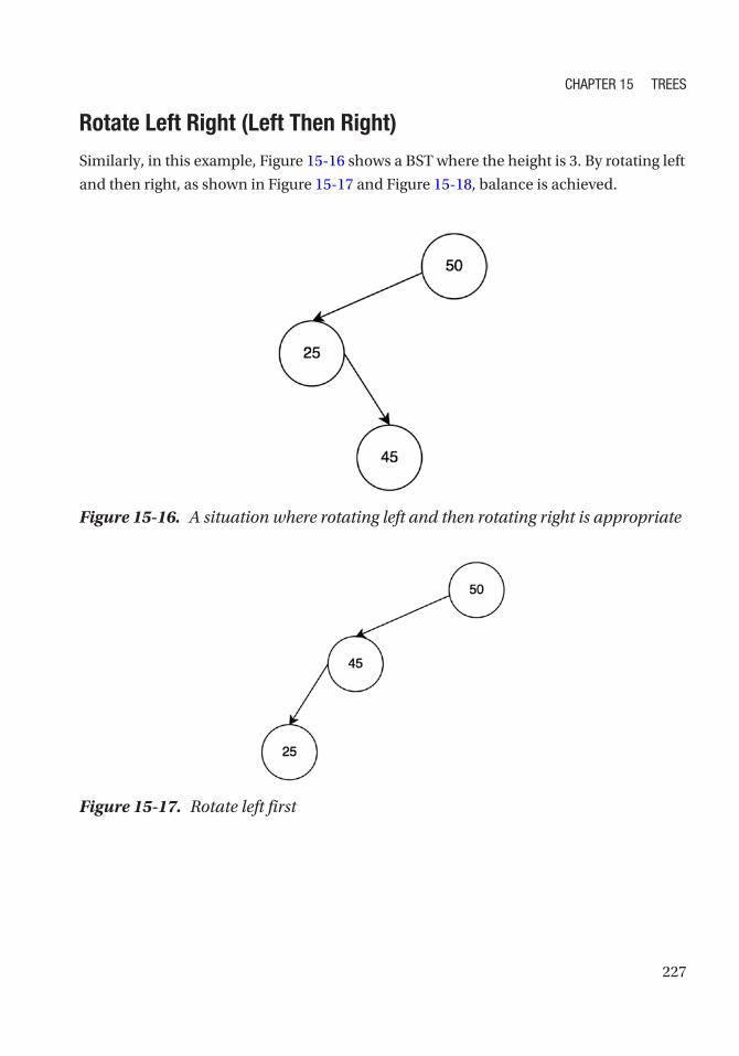
227
Rotate Left Right (Left Then Right)
Similarly, in this example, Figure 15-16 shows a BST where the height is 3. By rotating left
and then right, as shown in Figure 15-17 and Figure 15-18, balance is achieved.
Figure 15-16. A situation where rotating left and then rotating right is appropriate
Figure 15-17. Rotate left first
Chapter 15 trees

228
Balancing the TreeTo check for balance of the AVL tree, it is a simple comparison of the left and right
children’s heights. If the heights are not balanced, rotations are needed. When left is
bigger than right, left rotation is done. When right is bigger than left, right rotation is
done.
1 AVLTree.prototype.balance = function() {
2 var ldepth = this.left == null ? 0 : this.left.depth;
3 var rdepth = this.right == null ? 0 : this.right.depth;
4
5 if (ldepth > rdepth + 1) {
6 // LR or LL rotation
7 var lldepth = this.left.left == null ? 0 : this.left.left.depth;
8 var lrdepth = this.left.right == null ? 0 : this.left.right.depth;
9
10 if (lldepth < lrdepth) {
11 // LR rotation consists of a RR rotation of the left child
12 this.left.rotateRR();
13 // plus a LL rotation of this node, which happens anyway
14 }
15 this.rotateLL();
16 } else if (ldepth + 1 < rdepth) {
17 // RR or RL rorarion
18 var rrdepth = this.right.right == null ? 0 : this.right.right.depth;
19 var rldepth = this.right.left == null ? 0 : this.right.left.depth;
20
Figure 15-18. Rotate right after
Chapter 15 trees

229
21 if (rldepth > rrdepth) {
22 // RR rotation consists of a LL rotation of the right child
23 this.right.rotateLL();
24 // plus a RR rotation of this node, which happens anyway
25 }
26 this.rotateRR();
27 }
28 }
InsertionInsertion in AVL BST is the same as the insertion in normal BST except that, once
inserted, the parent must balance its children and set the right depth.
1 AVLTree.prototype.insert = function(value) {
2 var childInserted = false;
3 if (value == this.value) {
4 return false; // should be all unique
5 } else if (value < this.value) {
6 if (this.left == null) {
7 this.left = new AVLTree(value);
8 childInserted = true;
9 } else {
10 childInserted = this.left.insert(value);
11 if (childInserted == true) this.balance();
12 }
13 } else if (value > this.value) {
14 if (this.right == null) {
15 this.right = new AVLTree(value);
16 childInserted = true;
17 } else {
18 childInserted = this.right.insert(value);
19
20 if (childInserted == true) this.balance();
21 }
22 }
Chapter 15 trees
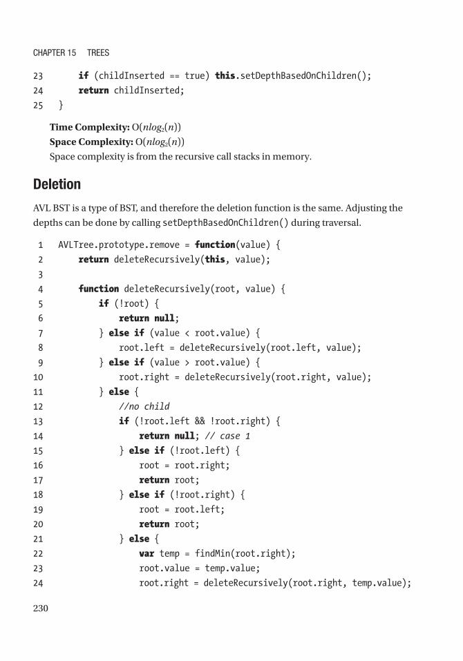
230
23 if (childInserted == true) this.setDepthBasedOnChildren();
24 return childInserted;
25 }
Time Complexity: O(nlog2(n))
Space Complexity: O(nlog2(n))
Space complexity is from the recursive call stacks in memory.
Deletion
AVL BST is a type of BST, and therefore the deletion function is the same. Adjusting the
depths can be done by calling setDepthBasedOnChildren() during traversal.
1 AVLTree.prototype.remove = function(value) {
2 return deleteRecursively(this, value);
3
4 function deleteRecursively(root, value) {
5 if (!root) {
6 return null;
7 } else if (value < root.value) {
8 root.left = deleteRecursively(root.left, value);
9 } else if (value > root.value) {
10 root.right = deleteRecursively(root.right, value);
11 } else {
12 //no child
13 if (!root.left && !root.right) {
14 return null; // case 1
15 } else if (!root.left) {
16 root = root.right;
17 return root;
18 } else if (!root.right) {
19 root = root.left;
20 return root;
21 } else {
22 var temp = findMin(root.right);
23 root.value = temp.value;
24 root.right = deleteRecursively(root.right, temp.value);
Chapter 15 trees
231
25 return root;
26 }
27 }
28 root.updateInNewLocation(); // ONLY DIFFERENCE from the BST one
29 return root;
30 }
31 function findMin(root) {
32 while (root.left) root = root.left;
33 return root;
34 }
35 }
The time complexity and space complexity are both O(nlog2(n)) because AVL trees
are balanced. The space complexity is from the recursive call stacks in memory.
Putting It All Together: AVL Tree ExampleWith the AVL tree class implemented, Figure 15-19 shows an example of an AVL tree
produced by the following code block:
1 var avlTest = new AVLTree(1,");
2 avlTest.insert(2);
3 avlTest.insert(3);
4 avlTest.insert(4);
5 avlTest.insert(5);
6 avlTest.insert(123);
7 avlTest.insert(203);
8 avlTest.insert(2222);
9 console.log(avlTest);
Chapter 15 trees

232
If a plain binary search tree were used instead, Figure 15-20 shows what it would
look like for the same order of insertion.
Figure 15-19. AVL result
Chapter 15 trees

233
Figure 15-20. BST result
Clearly, this is a skewed binary search tree that is completely unbalanced. At
this point, it looks like a linked list. Once the tree becomes completely unbalanced
like this, it has a linear time complexity for deletion, insertion, and search instead of
logarithmic time.
Chapter 15 trees
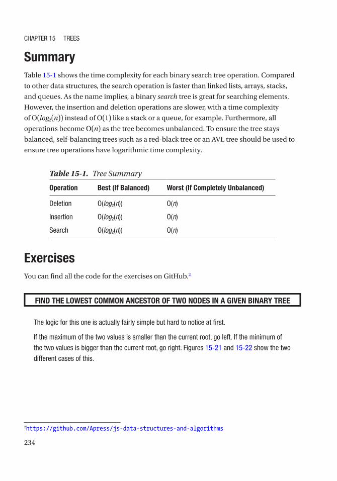
234
SummaryTable 15-1 shows the time complexity for each binary search tree operation. Compared
to other data structures, the search operation is faster than linked lists, arrays, stacks,
and queues. As the name implies, a binary search tree is great for searching elements.
However, the insertion and deletion operations are slower, with a time complexity
of O(log2(n)) instead of O(1) like a stack or a queue, for example. Furthermore, all
operations become O(n) as the tree becomes unbalanced. To ensure the tree stays
balanced, self-balancing trees such as a red-black tree or an AVL tree should be used to
ensure tree operations have logarithmic time complexity.
Table 15-1. Tree Summary
Operation Best (If Balanced) Worst (If Completely Unbalanced)
Deletion O(log2(n)) O(n)
Insertion O(log2(n)) O(n)
search O(log2(n)) O(n)
ExercisesYou can find all the code for the exercises on GitHub.2
FIND THE LOWEST COMMON ANCESTOR OF TWO NODES IN A GIVEN BINARY TREE
the logic for this one is actually fairly simple but hard to notice at first.
If the maximum of the two values is smaller than the current root, go left. If the minimum of
the two values is bigger than the current root, go right. Figures 15-21 and 15-22 show the two
different cases of this.
2 https://github.com/Apress/js-data-structures-and-algorithms
Chapter 15 trees
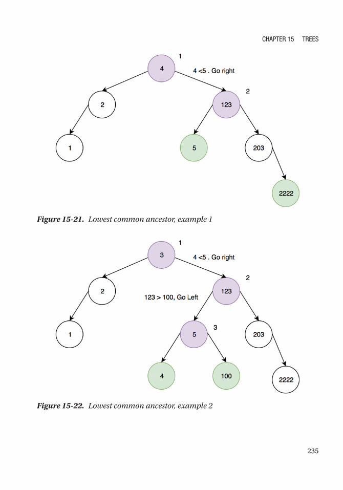
235
Figure 15-21. Lowest common ancestor, example 1
Figure 15-22. Lowest common ancestor, example 2
Chapter 15 trees

236
1 function findLowestCommonAncestor(root, value1, value2) {
2 function findLowestCommonAncestorHelper(root, value1, value2) {
3 if (!root)
4 return;
5 if (Math.max(value1, value2) < root.value)
6 return findLowestCommonAncestorHelper(root.left, value1, value2);
7 if (Math.min(value1, value2) > root.value)
8 return findLowestCommonAncestorHelper(root.right, value1, value2);
9 return root.value
10 }
11 return findLowestCommonAncestorHelper(root, value1, value2);
12 }
13 var node1 = {
14 value: 1,
15 left: {
16 value: 0
17 },
18 right: {
19 value: 2
20 }
21 }
22
23 var node2 = {
24 value: 1,
25 left: {
26 value: 0,
27 left: {
28 value: -1
29 },
30 right: {
31 value: 0.5
32 }
33 },
34 right: {
35 value: 2
36 }
37 }
Chapter 15 trees

237
38 console.log(findLowestCommonAncestor(node1, 0, 2)); // 1
39 console.log(findLowestCommonAncestor(node2, 0, 2)); // 1
40 console.log(findLowestCommonAncestor(node1, 0.5, -1)); // 0
Time Complexity: O(log2(n))
PRINT NODES NTH DISTANCE FROM THE ROOT
For this question, traverse the Bst in any way (level order was used in this example) and
check the height for each Bst node to see whether it should be printed.
1 function printKthLevels(root, k) {
2 var arrayKth = [];
3 queue = [];
4
5 if (!root) return;
6
7 // Breath first search for tree
8 queue.push([root, 0]);
9
10 while (queue.length) {
11 var tuple = queue.shift(),
12 temp = tuple[0],
13 height= tuple[1];
14
15 if (height == k) {
16 arrayKth.push(temp.value);
17 }
18 if (temp.left) {
19 queue.push([temp.left, height+1]);
20 }
21 if (temp.right) {
22 queue.push([temp.right,height+1]);
23 }
24 }
25 console.log(arrayKth);
26 }
Chapter 15 trees
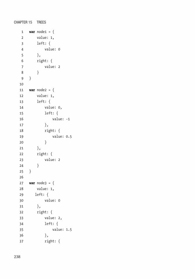
238
1 var node1 = {
2 value: 1,
3 left: {
4 value: 0
5 },
6 right: {
7 value: 2
8 }
9 }
10
11 var node2 = {
12 value: 1,
13 left: {
14 value: 0,
15 left: {
16 value: -1
17 },
18 right: {
19 value: 0.5
20 }
21 },
22 right: {
23 value: 2
24 }
25 }
26
27 var node3 = {
28 value: 1,
29 left: {
30 value: 0
31 },
32 right: {
33 value: 2,
34 left: {
35 value: 1.5
36 },
37 right: {
Chapter 15 trees

239
38 value: 3,
39 left: {
40 value: 3.25
41 }
42 }
43 }
44 }
45
46 printKthLevels(node1, 1); // 1
47 printKthLevels(node1, 2); // [0,2]
CHECK WHETHER A BINARY TREE IS A SUBTREE OF ANOTHER TREE
to do this, traverse the binary tree in any way (I’m choosing to do level order) and check
whether the one that it is currently on is the same as the subtree.
1 function isSameTree(root1, root2) {
2 if (root1 == null && root2 == null) {
3 return true;
4 }
5 if (root1 == null || root2 == null) {
6 return false;
7 }
8
9 return root1.value == root2.value &&
10 isSameTree(root1.left, root2.left) &&
11 isSameTree(root1.right, root2.right)
12 }
13
14 function checkIfSubTree(root, subtree) {
15 // Breath first search
16 var queue = [],
17 counter = 0;
18
19 // sanity check for root
20 if (!root) {
21 return;
Chapter 15 trees

240
22 }
23
24 queue.push(root);
25
26 while (queue.length) {
27 var temp = queue.shift();
28
29 if (temp.data == subtree.data == isSameTree(temp, subtree)) {
30 return true;
31 }
32
33 if (temp.left) {
34 queue.push(temp.left);
35 }
36 if (temp.right) {
37 queue.push(temp.right);
38 }
39 }
40 return false;
41 }
42
43 var node1 = {
44 value: 5,
45 left: {
46 value: 3,
47 left: {
48 value: 1
49 },
50 right: {
51 value: 2
52 }
53 },
54 right: {
55 value: 7
56 }
57 }
58
Chapter 15 trees

241
59 var node2 = {
60 value: 3,
61 left: {
62 value: 1
63 },
64 right: {
65 value: 2
66 }
67 }
68
69
70 var node3 = {
71 value: 3,
72 left: {
73 value: 1
74 }
75 }
76
77 console.log(checkIfSubTree(node1, node2)); // true
78 console.log(checkIfSubTree(node1, node3)); // false
79 console.log(checkIfSubTree(node2, node3)); // false
CHECK WHETHER A TREE IS A MIRROR OF ANOTHER TREE
Figure 15-23 shows an example.
Figure 15-23. Mirror trees
Chapter 15 trees

242
here are three possible cases:
• their root node’s key must be the same.
• the left subtree of root of a and the right subtree root of b are mirrors.
• the right subtree of a and the left subtree of b are mirrors.
1 function isMirrorTrees(tree1, tree2) {
2 // Base case, both empty
3 if (!tree1 && !tree2) {
4 return true;
5 }
6
7 // One of them is empty, since only one is empty, not mirrored
8 if (!tree1 || !tree2) {
9 return false;
10 }
11
12 // Both non-empty, compare them recursively.
13 // Pass left of one and right of the other
14
15 var checkLeftwithRight = isMirrorTrees(tree1.left, tree2.right),
16 checkRightwithLeft = isMirrorTrees(tree2.right, tree1.left);
17
18 return tree1.value == tree2.value && checkLeftwithRight &&
checkRightwithLeft;
19 }
20
21 var node1 = {
22 value: 3,
23 left: {
24 value: 1
25 },
26 right: {
27 value: 2
28 }
29 }
30
Chapter 15 trees
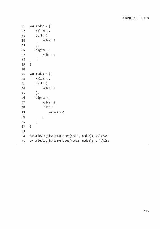
243
31 var node2 = {
32 value: 3,
33 left: {
34 value: 2
35 },
36 right: {
37 value: 1
38 }
39 }
40
41 var node3 = {
42 value: 3,
43 left: {
44 value: 1
45 },
46 right: {
47 value: 2,
48 left: {
49 value: 2.5
50 }
51 }
52 }
53
54 console.log(isMirrorTrees(node1, node2)); // true
55 console.log(isMirrorTrees(node2, node3)); // false
Chapter 15 trees

245© Sammie Bae 2019 S. Bae, JavaScript Data Structures and Algorithms, https://doi.org/10.1007/978-1-4842-3988-9_16
CHAPTER 16
HeapsThis chapter will introduce heaps. A heap is an important data structure that returns the
highest or lowest element in O(1) time. This chapter will focus on explaining how heaps
are implemented as well as how to work with them. One example is heap sort, which is a
sorting algorithm based on heaps.
Understanding HeapsA heap is a type of tree-like data structure in which the parent is bigger than its children
(if max-heap) or smaller than its children (if min-heap). This property of the heap makes
it useful for sorting data.
Heaps, unlike other tree data structures, use an array to store data instead of
having pointers to their children. A heap node’s children’s positions (indices) in the
array can be calculated easily. This is because the parent-child relationship is easily
defined with a heap.
There are many types of heaps that have different numbers of children. In this
chapter, only binary heaps will be considered. Since a heap uses an array to store the
data, the indices of the array define the order/height of each element. A binary heap can
be built by placing the first array element as the root and then filling each left and right
element in order.
For example, for the heap shown in Figure 16-1, the array would look like this:
[2, 4, 23, 12, 13].

246
There are two types of binary heaps: max-heap and min-heap. In max-heap, the
root node has the highest value, and each node’s value is greater than its children. In
min-heap, the root node has the lowest value, and each node’s value is smaller than its
children.
Heaps can store any values of any type: strings, integer, and even custom classes. As
covered in Chapters 3 and 4, strings and integer value comparisons are handled natively
by JavaScript (e.g., 9 is greater than 1, z is greater than a). However, for custom classes,
the developer needs to implement a way to compare two classes. This chapter will look
at heaps that store integer values only.
Max-HeapA max-heap is a heap where the parent is always greater than any of its children
(see Figure 16-2).
Figure 16-1. Heap indices
Chapter 16 heaps

247
Here is the array for the max-heap shown in Figure 16-2: [100, 19, 36, 17, 3, 25, 1, 2, 7].
Min-HeapA min-heap is a heap where the parent is always smaller than any of its children
(see Figure 16-3).
Figure 16-2. Max-heap
Figure 16-3. Min-heap
Chapter 16 heaps

248
Here is the array for the max-heap shown in Figure 16-3: [1, 2, 3, 17, 19, 36, 7, 25, 100].
Binary Heap Array Index StructureFor a binary heap, an array is used to represent the heap by using the following indices,
where N is the index of the node:
Node Index
(itself) N
Parent (N-1) / 2
Left Child (N*2) + 1
Right Child (N*2) + 2
Figure 16-4 illustrates this familial relationship using indices.
Figure 16-4. Heap relationship
Chapter 16 heaps

249
Let’s first define a generic Heap class. An array will be used to store all the values
using the index structure described earlier. The following heap class implements helper
functions that retrieve the parent node, the left child, and the right child. The following
code block has a peek function that returns the maximum value for a max-heap and the
minimum value for a min-heap.
1 function Heap() {
2 this.items = [];
3 }
4
5 Heap.prototype.swap = function(index1, index2) {
6 var temp = this.items[index1];
7 this.items[index1] = this.items[index2];
8 this.items[index2] = temp;
9 }
10
11 Heap.prototype.parentIndex = function(index) {
12 return Math.floor((index - 1) / 2);
13 }
14
15 Heap.prototype.leftChildIndex = function(index) {
16 return index * 2 + 1;
17 }
18
19 Heap.prototype.rightChildrenIndex = function(index) {
20 return index * 2 + 2;
21 }
22
23 Heap.prototype.parent = function(index) {
24 return this.items[this.parentIndex(index)];
25 }
26
27 Heap.prototype.leftChild = function(index) {
28 return this.items[this.leftChildIndex(index)];
29 }
30
Chapter 16 heaps
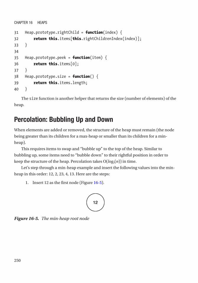
250
31 Heap.prototype.rightChild = function(index) {
32 return this.items[this.rightChildrenIndex(index)];
33 }
34
35 Heap.prototype.peek = function(item) {
36 return this.items[0];
37 }
38 Heap.prototype.size = function() {
39 return this.items.length;
40 }
The size function is another helper that returns the size (number of elements) of the
heap.
Percolation: Bubbling Up and DownWhen elements are added or removed, the structure of the heap must remain (the node
being greater than its children for a max-heap or smaller than its children for a min-
heap).
This requires items to swap and “bubble up” to the top of the heap. Similar to
bubbling up, some items need to “bubble down” to their rightful position in order to
keep the structure of the heap. Percolation takes O(log2(n)) in time.
Let’s step through a min-heap example and insert the following values into the min-
heap in this order: 12, 2, 23, 4, 13. Here are the steps:
1. Insert 12 as the first node (Figure 16-5).
Figure 16-5. The min-heap root node
Chapter 16 heaps

251
2. Insert a new 2 node (Figure 16-6).
Figure 16-6. The newest node is smaller than the parent
3. The 2 node bubbles up because it is smaller than 12 and hence
should be on the top of the min-heap (Figure 16-7).
Figure 16-7. The smaller node has bubbled up to the parent position
4. Insert a new 23 node in the second child position (Figure 16-8).
Figure 16-8. The larger 23 node remains in place in the min-heap structure
Chapter 16 heaps

252
5. Insert 4 in the heap, as in Figure 16-9.
Figure 16-9. The new node in the min-heap is smaller than the one above it
6. 12 is swapped with 4 to maintain the min-heap structure (Figure 16-10).
Figure 16-10. The smaller 4 node has bubbled up to maintain the min-heap structure
Chapter 16 heaps

253
7. Insert 13, as in Figure 16-11.
Figure 16-11. The newest and larger 13 node remains in place
Here is the array content for this heap: [2, 4, 23, 12, 13].
Implementing PercolationTo implement the “bubbling up and down” of percolation, swap until the min-heap
structure is formed with the minimum element on the top. For bubbling down, swap the
top element (first in the array) with one of its children if that child is smaller. Likewise,
for bubbling up, swap the new element with its parent if the parent is greater than the
new element.
1 function MinHeap() {
2 this.items = [];
3 }
4 MinHeap.prototype = Object.create(Heap.prototype);
// inherit helpers from heap by copying prototype
5 MinHeap.prototype.bubbleDown = function() {
6 var index = 0;
Chapter 16 heaps

254
7 while (this.leftChild(index) && this.leftChild(index) < this.
items[index]) {
8 var smallerIndex = this.leftChildIndex(index);
9 if (this.rightChild(index)
10 && this.rightChild(index) < this.items[smallerIndex]) {
11 // if right is smaller, right swaps
12 smallerIndex = this.rightChildrenIndex(index);
13 }
14 this.swap(smallerIndex, index);
15 index = smallerIndex;
16 }
17 }
18
19 MinHeap.prototype.bubbleUp = function() {
20 var index = this.items.length - 1;
21 while (this.parent(index) && this.parent(index) > this.items[index]) {
22 this.swap(this.parentIndex(index), index);
23 index = this.parentIndex(index);
24 }
25 }
A max-heap implementation differs only in the comparators. For bubbling down, the
max-heap node swaps with one of its children if the child is greater. Likewise, for bubbling
up, the newest node swaps with its parent if its parent is smaller than the new node.
Max-Heap ExampleLet’s build a max-heap now with the same values as the one used in the previous min-
heap example by inserting the following values in the order: 12, 2, 23, 4, 13.
1. Insert the first node, which is 12 (Figure 16-12).
Figure 16-12. The first max-heap node
Chapter 16 heaps

255
2. Insert a new 2 node (Figure 16-13).
3. Insert 23, as in Figure 16-14.
4. The 23 node “bubbles” to the top to maintain max-heap structure
(Figure 16-15).
Figure 16-13. The new smaller node remains in place in the max-heap structure
Figure 16-14. The new child node is larger than the parent
Figure 16-15. The new larger node is swapped with the smaller 12
Chapter 16 heaps

256
5. Insert 4, as in Figure 16-16.
6. To maintain the max-heap structure, 4 bubbles up, and 2 bubbles
down (Figure 16- 17).
Figure 16-16. The new node is larger than the one above it
Figure 16-17. The 4 and 2 nodes swap places
Chapter 16 heaps

257
7. Insert 13, as in Figure 16-18.
8. Because of the max-heap structure, 13 and 4 swap positions
(Figure 16-19).
Here is the array content for this heap: [23, 13, 12, 2, 4].
Figure 16-18. The new node is larger than the one above it
Figure 16-19. Percolation restores the max-heap structure
Chapter 16 heaps

258
Min-Heap Complete ImplementationPutting all the functions defined together and inheriting Heap’s functions, the complete
implementation and example of min-heap is shown next. The add and poll functions
were added. add simply adds a new element to the heap, but bubbleUp ensures that this
element in the min-heap satisfies the order. poll removes the minimum element (the
root) from the heap and calls bubbleDown to keep the min-heap order.
1 function MinHeap() {
2 this.items = [];
3 }
4 MinHeap.prototype = Object.create(Heap.prototype); // inherit helpers
from heap by copying prototype
5 MinHeap.prototype.add = function(item) {
6 this.items[this.items.length] = item;
7 this.bubbleUp();
8 }
9
10 MinHeap.prototype.poll = function() {
11 var item = this.items[0];
12 this.items[0] = this.items[this.items.length - 1];
13 this.items.pop();
14 this.bubbleDown();
15 return item;
16 }
17
18 MinHeap.prototype.bubbleDown = function() {
19 var index = 0;
20 while (this.leftChild(index) && (this.leftChild(index) < this.
items[index] || this.rightChild(index) < this.items[index]) ) {
21 var smallerIndex = this.leftChildIndex(index);
22 if (this.rightChild(index) && this.rightChild(index) < this.
items[smallerIndex]) {
23 smallerIndex = this.rightChildrenIndex(index);
24 }
25 this.swap(smallerIndex, index);
Chapter 16 heaps

259
26 index = smallerIndex;
27 }
28 }
29
30 MinHeap.prototype.bubbleUp = function() {
31 var index = this.items.length - 1;
32 while (this.parent(index) && this.parent(index) > this.
items[index]) {
33 this.swap(this.parentIndex(index), index);
34 index = this.parentIndex(index);
35 }
36 }
37
38 var mh1 = new MinHeap();
39 mh1.add(1);
40 mh1.add(10);
41 mh1.add(5);
42 mh1.add(100);
43 mh1.add(8);
44
45 console.log(mh1.poll()); // 1
46 console.log(mh1.poll()); // 5
47 console.log(mh1.poll()); // 8
48 console.log(mh1.poll()); // 10
49 console.log(mh1.poll()); // 100
Max-Heap Complete ImplementationAs previously discussed, the only difference between the min-heap and max-heap
implementations is the comparator in bubbleDown and bubbleUp. With the same
elements added as the previous example, meaning (1, 10, 5, 100, 8), the max-heap
returns the highest elements when poll is called.
1 function MaxHeap() {
2 this.items = [];
3 }
Chapter 16 heaps

260
4 MaxHeap.prototype = Object.create(Heap.prototype);
// inherit helpers from heap by copying prototype
5 MaxHeap.prototype.poll = function() {
6 var item = this.items[0];
7 this.items[0] = this.items[this.items.length - 1];
8 this.items.pop();
9 this.bubbleDown();
10 return item;
11 }
12
13 MaxHeap.prototype.bubbleDown = function() {
14 var index = 0;
15 while (this.leftChild(index) && (this.leftChild(index) > this.
items[index] || this.rightChild(index) > this.items[index] ) ) {
16 var biggerIndex = this.leftChildIndex(index);
17 if (this.rightChild(index) && this.rightChild(index) > this.
items[bigger\Index])
18 {
19 biggerIndex = this.rightChildrenIndex(index);
20 }
21 this.swap(biggerIndex, index);
22 index = biggerIndex;
23 }
24 }
25
26 MaxHeap.prototype.bubbleUp = function() {
27 var index = this.items.length - 1;
28 while (this.parent(index) && this.parent(index) < this.
items[index]) {
29 this.swap(this.parentIndex(index), index);
30 index = this.parentIndex(index);
31 }
32 }
33
Chapter 16 heaps

261
34 var mh2 = new MaxHeap();
35 mh2.add(1);
36 mh2.add(10);
37 mh2.add(5);
38 mh2.add(100);
39 mh2.add(8);
40
41 console.log(mh2.poll()); // 100
42 console.log(mh2.poll()); // 10
43 console.log(mh2.poll()); // 8
44 console.log(mh2.poll()); // 5
45 console.log(mh2.poll()); // 1
Heap SortNow that heap classes have been created, sorting with a heap is fairly straightforward.
To get a sorted array, simply call .pop() on the heap until it is empty and store the stored
popped objects. This is as known as a heap sort. Since percolation takes O(log2(n)),
and sorting must pop n number of elements, the time complexity for a heap sort is
O(nlog2(n)), like quicksort and mergesort.
In this section, we will first do an ascending sort implemented using a min-heap and
then a descending sort implemented using a max-heap.
Ascending-Order Sort (Min-Heap)Figure 16-20 shows the min-heap when all the items have been added to the min-heap,
and Figures 16-21 to 16-23 show the heap restructuring as items are popped. Finally,
when it is empty, the sort is complete.
Chapter 16 heaps

262
1 var minHeapExample = new MinHeap();
2 minHeapExample.add(12);
3 minHeapExample.add(2);
4 minHeapExample.add(23);
5 minHeapExample.add(4);
6 minHeapExample.add(13);
7 minHeapExample.items; // [2, 4, 23, 12, 13]
8
9 console.log(minHeapExample.poll()); // 2
10 console.log(minHeapExample.poll()); // 4
11 console.log(minHeapExample.poll()); // 12
12 console.log(minHeapExample.poll()); // 13
13 console.log(minHeapExample.poll()); // 23
The last node (where 13 used to be) is removed, and then 13 is placed on the top.
Through the percolation process, 13 moves down to after the left child of 12 since it’s
bigger than both 4 and 13.
Figure 16-20. Min-heap sort after all items added
Chapter 16 heaps
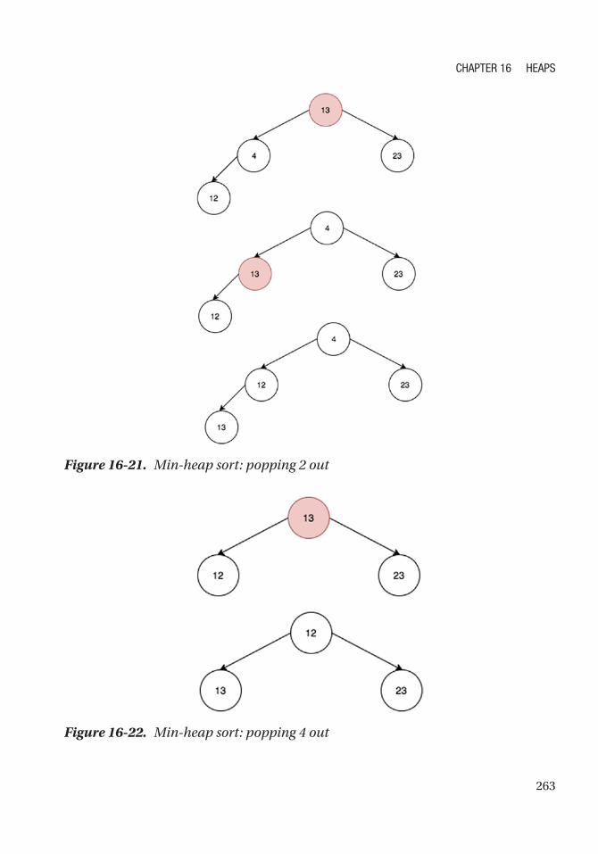
263
Figure 16-21. Min-heap sort: popping 2 out
Figure 16-22. Min-heap sort: popping 4 out
Chapter 16 heaps

264
Descending-Order Sort (Max-Heap)Figure 16-24 shows the max-heap when all the items have been added to the min-heap,
and Figures 16-25 through 16-27 show the max-heap restructuring as items are popped.
Finally, when it is empty, the sort is complete.
Figure 16-24. Max-heap sort after all items are added
Figure 16-23. Min-heap sort: popping 12 out
1 var maxHeapExample = new MaxHeap();
2 maxHeapExample.add(12);
3 maxHeapExample.add(2);
4 maxHeapExample.add(23);
5 maxHeapExample.add(4);
6 maxHeapExample.add(13);
Chapter 16 heaps

265
7 maxHeapExample.items; // [23, 13, 12, 2, 4]
8
9 console.log(maxHeapExample.poll()); // 23
10 console.log(maxHeapExample.poll()); // 13
11 console.log(maxHeapExample.poll()); // 12
12 console.log(maxHeapExample.poll()); // 2
13 console.log(maxHeapExample.poll()); // 4
Figure 16-25. Max sort: popping 23 out
Chapter 16 heaps

266
Figure 16-27. Max sort: popping 12 out
Figure 16-26. Max sort: popping 13 out
Chapter 16 heaps

267
Heaps maintain their structure via percolation; when a node is inserted, it “bubbles
up” by repeatedly swapping with elements until the proper heap structure is achieved.
For a min-heap, this means the lowest-valued node at the root. For a max-heap, this
means the highest-valued node at the root. Heaps work fundamentally by percolation,
which allows deletion and insertion in O(log2(n)) time, as summarized in Table 16-2.
SummaryA heap is a tree-like data structure represented using arrays. To get the parent, left child,
and right child of a tree’s node, you can use the index formula in Table 16-1.
Table 16-1. Heap Node Index Summary
Node Index
(self) N
parent (N-1) / 2
Left child (N*2) + 1
right child (N*2) + 2
Table 16-2. Heap Operations Summary
Operation Time Complexity
Deletion (leads to “bubble down”) O(log2(n))
Insertion (leads to “bubble up”) O(log2(n))
heap sort O(n log2(n))
Chapter 16 heaps

268
ExercisesYou can find all the code for the exercises on GitHub.1
KEEP TRACK OF MEDIAN IN STREAM OF NUMBERS
since this question is in this chapter, that’s already a big hint for approaching it. In theory,
the solution is fairly simple. have one min-heap and one max-heap, and then retrieving the
median takes only O(1).
For example, let’s have a stream of the following integers: 12, 2, 23, 4, 13.
Median, when 12 is inserted, is 12 since that’s the only element. When 2 is inserted, there is
an even number of items: 2 and 12. hence, the median is its arithmetic mean, 7 ((12+2)/2).
When 23 is inserted, the median is 12. Finally, when 13 is inserted, the median is 12.5, the
average of two middle terms (12 and 13).
1 medianH.push(12);
2 console.log(medianH.median()); // 12
3 medianH.push(2);
4 console.log(medianH.median()); // 7 ( because 12 + 2 = 14; 14/2 = 7)
5 medianH.push(23);
6 console.log(medianH.median()); // 12
7 medianH.push(13);
8 console.log(medianH.median()); // 12.5
1 function MedianHeap() {
2 this.minHeap = new MinHeap();
3 this.maxHeap = new MaxHeap();
4 }
5
6 MedianHeap.prototype.push = function (value) {
7 if (value > this.median()) {
8 this.minHeap.add(value);
9 } else {
10 this.maxHeap.add(value);
11 }
1 https://github.com/Apress/js-data-structures-and-algorithms
Chapter 16 heaps

269
12
13 // Re balancing
14 if (this.minHeap.size() - this.maxHeap.size() > 1) {
15 this.maxHeap.push(this.minHeap.poll());
16 }
17
18 if (this.maxHeap.size() - this.minHeap.size() > 1){
19 this.minHeap.push(this.maxHeap.poll());
20 }
21 }
22
23 MedianHeap.prototype.median = function () {
24 if (this.minHeap.size() == 0 && this.maxHeap.size() == 0){
25 return Number.NEGATIVE_INFINITY;
26 } else if (this.minHeap.size() == this.maxHeap.size()) {
27 return (this.minHeap.peek() + this.maxHeap.peek()) / 2;
28 } else if (this.minHeap.size() > this.maxHeap.size()) {
29 return this.minHeap.peek();
30 } else {
31 return this.maxHeap.peek();
32 }
33 }
34
35 var medianH = new MedianHeap();
36
37 medianH.push(12);
38 console.log(medianH.median()); // 12
39 medianH.push(2);
40 console.log(medianH.median()); // 7 ( because 12 + 2 = 14; 14/2 = 7)
41 medianH.push(23);
42 console.log(medianH.median()); // 12
43 medianH.push(13);
44 console.log(medianH.median()); // 12.5
Chapter 16 heaps

270
FIND THE K TH SMALLEST VALUE IN AN ARRAY
this problem has been explored before in Chapter 10 using quicksort’s helper function.
another way to do it is to use a heap. simply add the elements into a heap and pop it kth
times. By definition of min-heaps, this returns the kth smallest value in the array.
1 var array1 = [12, 3, 13, 4, 2, 40, 23]
2
3 function getKthSmallestElement(array, k) {
4 var minH = new MinHeap();
5 for (var i = 0, arrayLength = array.length; i < arrayLength; i++) {
6 minH.add(array[i]);
7 }
8 for (var i = 1; i < k; i++) {
9 minH.poll();
10 }
11 return minH.poll();
12 }
13 getKthSmallestElement(array1, 2); // 3
14 getKthSmallestElement(array1, 1); // 2
15 getKthSmallestElement(array1, 7); // 40
FIND THE KTH LARGEST VALUE IN AN ARRAY
this is the same idea from before just with max-heap.
1 var array1 = [12,3,13,4,2,40,23];
2
3 function getKthBiggestElement(array, k) {
4 var maxH = new MaxHeap();
5 for (var i=0, arrayLength = array.length; i<arrayLength; i++) {
6 maxH.push(array[i]);
7 }
8 for (var i=1; i<k; i++) {
9 maxH.pop();
10 }
Chapter 16 heaps

271
11 return maxH.pop();
12 }
13 getKthBiggestElement(array1,2); // 23
14 getKthBiggestElement(array1,1); // 40
15 getKthBiggestElement(array1,7); // 2
Time Complexity: O(klog2(n))
here, n is the size of the array since each .pop costs O(log2(n)), which has to be done k times.
Space Complexity: O(n)
O(n) in memory is needed to store the heap array.
Chapter 16 heaps

273© Sammie Bae 2019 S. Bae, JavaScript Data Structures and Algorithms, https://doi.org/10.1007/978-1-4842-3988-9_17
CHAPTER 17
GraphsThis chapter covers graphs. Graphs are a versatile way of representing connections
between objects. In this chapter, you will learn graph basics, including fundamental
terminology and graph types. The chapter will also cover working with these different
graph types and methods of representing graphs in data structures that have already
been explored. Finally, algorithms for traversing, searching, and sorting graphs are
explored to solve problems such as finding the shortest path between two graph nodes.
Graph BasicsAs mentioned in the introduction, graphs are visual representations of the connections
between objects. Such representations can be of many things and have different
applications; Table 17-1 shows some examples.
Table 17-1. Examples of Graph Applications
Application Item Connection
Web site Web page Links
Map Intersection Road
Circuit Component Wiring
Social media Person “Friendship”/connection
Telephone Phone number Landline

274
Figure 17-1 shows two examples of simple graphs.
Figure 17-1. Two examples of graphs
Before we delve into graphs too deeply, it is useful to introduce some basic
terminology and concepts.
• Vertex: A vertex is the node from which graphs are formed. In this
chapter, a node will be noted as V for Big-O analysis. A vertex is
represented using a circle, as shown in Figure 17-2.
• Edge: An edge is the connection between nodes in a graph.
Graphically, it is the “line” between the vertices. It will be noted as E
for Big-O analysis. An edge is represented using a line, as shown in
Figure 17-2.
ChaPTeR 17 GRaPhS

275
• Degree of vertex: The degree of a vertex refers to the number of edges
on that vertex (node).
• Sparse graph: A graph is considered sparse when only a small fraction
of possible connections exist between vertices (see Figure 17-3).
Figure 17-2. Vertices and edges
Figure 17-3. Sparse graph
ChaPTeR 17 GRaPhS
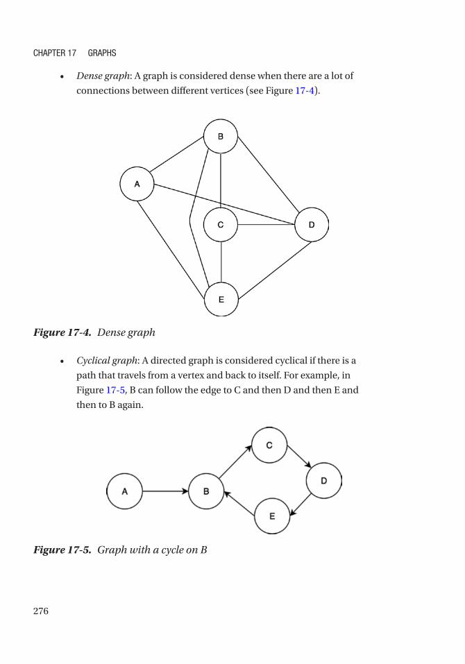
276
• Dense graph: A graph is considered dense when there are a lot of
connections between different vertices (see Figure 17-4).
Figure 17-4. Dense graph
• Cyclical graph: A directed graph is considered cyclical if there is a
path that travels from a vertex and back to itself. For example, in
Figure 17-5, B can follow the edge to C and then D and then E and
then to B again.
Figure 17-5. Graph with a cycle on B
ChaPTeR 17 GRaPhS
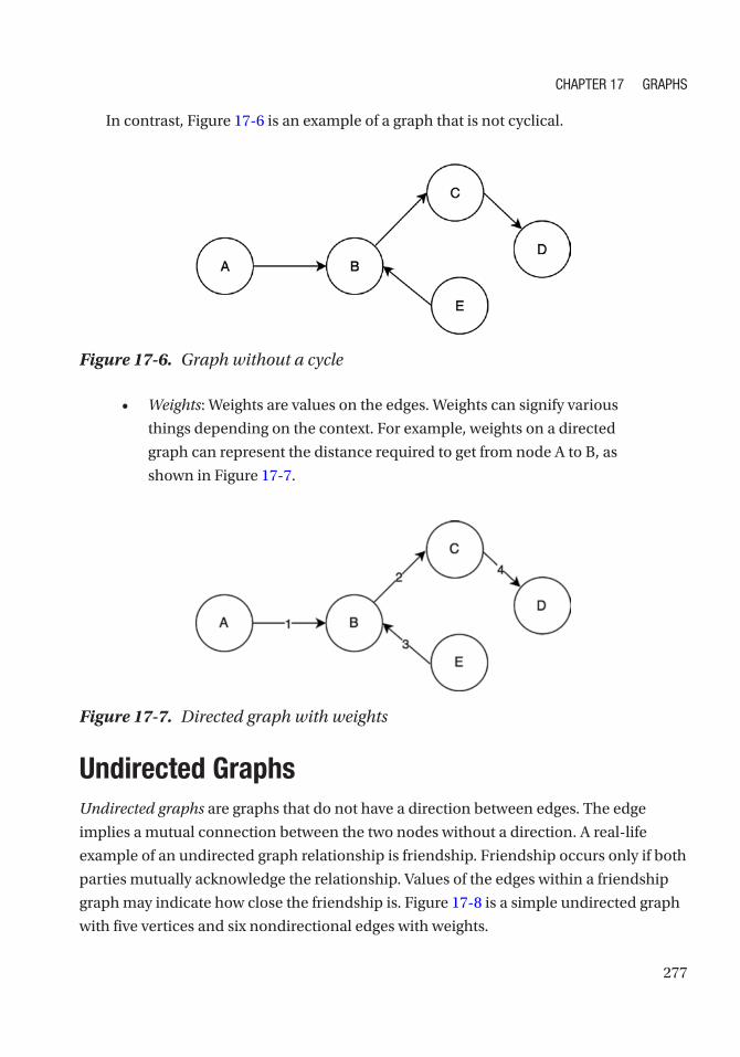
277
In contrast, Figure 17-6 is an example of a graph that is not cyclical.
Figure 17-6. Graph without a cycle
• Weights: Weights are values on the edges. Weights can signify various
things depending on the context. For example, weights on a directed
graph can represent the distance required to get from node A to B, as
shown in Figure 17-7.
Figure 17-7. Directed graph with weights
Undirected GraphsUndirected graphs are graphs that do not have a direction between edges. The edge
implies a mutual connection between the two nodes without a direction. A real-life
example of an undirected graph relationship is friendship. Friendship occurs only if both
parties mutually acknowledge the relationship. Values of the edges within a friendship
graph may indicate how close the friendship is. Figure 17-8 is a simple undirected graph
with five vertices and six nondirectional edges with weights.
ChaPTeR 17 GRaPhS

278
There are various ways to represent undirected graphs as a data structure class.
Two of the most common ways to do this are by using an adjacency matrix or an
adjacency list. The adjacency list uses a vertex as the key for nodes with its neighbors
stored into a list, whereas an adjacency matrix is a V by V matrix with each element
of the matrix indicating a connection between two vertices. Figure 17-9 illustrates the
difference between an adjacency list and an adjacency matrix (This book covers only
adjacency lists).
Figure 17-8. Undirected graph with weights
Figure 17-9. Graph (left), adjacency list (middle), and adjacency matrix (right)
ChaPTeR 17 GRaPhS
279
So far, the concepts and definitions of graphs have been discussed. Now, let’s
actually start implementing these ideas into code and learn how to add and remove
edges and vertices.
Adding Edges and VerticesIn this example, we create a weighted undirected graph and add vertices and edges. First,
we’ll create a new class for an undirected graph. The undirected graph should have an
object to store the edges. This is implemented as shown in the following code block:
1 function UndirectedGraph() {
2 this.edges = {};
3 }
To add edges, vertices (nodes) must be added first. This implementation will take
the adjacency list approach by having vertices as objects inside the this.edges object in
which edge values are stored.
1 UndirectedGraph.prototype.addVertex = function(vertex) {
2 this.edges[vertex] = {};
3 }
To add weighted edges into the undirected graph, both vertices in the this.edges
objects are used to set the weight.
1 UndirectedGraph.prototype.addEdge = function(vertex1,vertex2, weight)
{
2 if (weight == undefined) {
3 weight = 0;
4 }
5 this.edges[vertex1][vertex2] = weight;
6 this.edges[vertex2][vertex1] = weight;
7 }
With this, let’s add some vertices and edges with the following code:
1 var graph1 = new UndirectedGraph();
2 graph1.addVertex(1);
3 graph1.addVertex(2);
ChaPTeR 17 GRaPhS
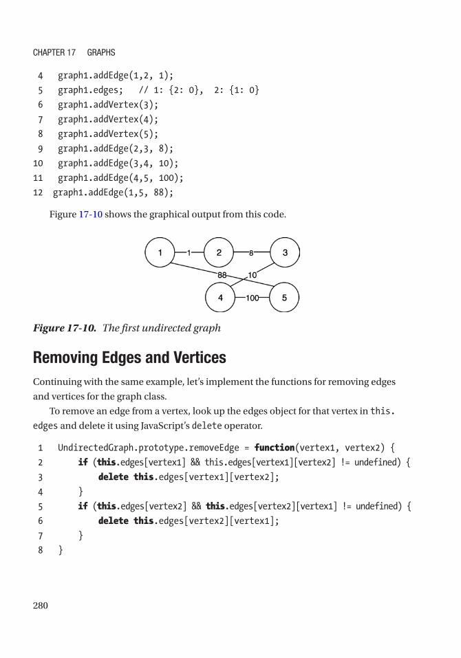
280
4 graph1.addEdge(1,2, 1);
5 graph1.edges; // 1: {2: 0}, 2: {1: 0}
6 graph1.addVertex(3);
7 graph1.addVertex(4);
8 graph1.addVertex(5);
9 graph1.addEdge(2,3, 8);
10 graph1.addEdge(3,4, 10);
11 graph1.addEdge(4,5, 100);
12 graph1.addEdge(1,5, 88);
Figure 17-10 shows the graphical output from this code.
Figure 17-10. The first undirected graph
Removing Edges and VerticesContinuing with the same example, let’s implement the functions for removing edges
and vertices for the graph class.
To remove an edge from a vertex, look up the edges object for that vertex in this.
edges and delete it using JavaScript’s delete operator.
1 UndirectedGraph.prototype.removeEdge = function(vertex1, vertex2) {
2 if (this.edges[vertex1] && this.edges[vertex1][vertex2] != undefined) {
3 delete this.edges[vertex1][vertex2];
4 }
5 if (this.edges[vertex2] && this.edges[vertex2][vertex1] != undefined) {
6 delete this.edges[vertex2][vertex1];
7 }
8 }
ChaPTeR 17 GRaPhS

281
Next, let’s delete an entire vertex. One important point to remember is that any
time a vertex is removed, all edges connected to it also must be removed. This can be
accomplished using a loop, as shown in the following implementation:
1 UndirectedGraph.prototype.removeVertex = function(vertex) {
2 for (var adjacentVertex in this.edges[vertex]) {
3 this.removeEdge(adjacentVertex, vertex);
4 }
5 delete this.edges[vertex];
6 }
With removal now implemented, let’s create another undirected graph object similar
to the first example but delete some vertices and edges. Vertex 5 is removed first, and
the result is shown in Figure 17-11. Vertex 1 is also removed, as shown in Figure 17-12.
Finally, Figure 17-13 shows the result when the edge between 2 and 3 is removed.
1 var graph2 = new UndirectedGraph();
2 graph2.addVertex(1);
3 graph2.addVertex(2);
4 graph2.addEdge(1,2, 1);
5 graph2.edges; // 1: {2: 0}, 2: {1: 0}
6 graph2.addVertex(3);
7 graph2.addVertex(4);
8 graph2.addVertex(5);
9 graph2.addEdge(2,3, 8);
10 graph2.addEdge(3,4, 10);
11 graph2.addEdge(4,5, 100);
12 graph2.addEdge(1,5, 88);
13 graph2.removeVertex(5);
14 graph2.removeVertex(1);
15 graph2.removeEdge(2,3);
ChaPTeR 17 GRaPhS

282
Directed GraphsDirected graphs are graphs that do have a direction between vertices. Each edge in a
directed graph goes from one vertex to another, as shown in Figure 17-14.
Figure 17-11. Vertex 5 removed
Figure 17-12. Vertex 1 removed
Figure 17-13. Edge between 2 and 3 removed
ChaPTeR 17 GRaPhS

283
In this example, the E node can “travel” to the D node, and the D node can travel
only to the C node.
Now let’s implement a weighted directed graph class. The similar adjacency
list approach used in the undirected graph implementation will be used. First, the
DirectedGraph class is defined with the edges property as shown, and the method of
adding the vertex is the same as the implementation from the undirected graph class.
1 function DirectedGraph() {
2 this.edges = {};
3 }
4 DirectedGraph.prototype.addVertex = function (vertex) {
5 this.edges[vertex] = {};
6 }
Given an edge that starts at the origin vertex and ends at the destination vertex, to
add edges into the directed graph, the weight should be set only on the origin vertex, as
shown here:
1 DirectedGraph.prototype.addEdge = function(origVertex, destVertex, weight) {
2 if (weight === undefined) {
3 weight = 0;
Figure 17-14. Directed graph
ChaPTeR 17 GRaPhS
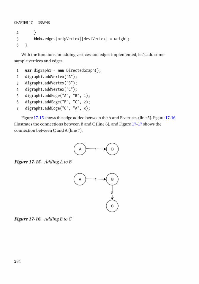
284
4 }
5 this.edges[origVertex][destVertex] = weight;
6 }
With the functions for adding vertices and edges implemented, let’s add some
sample vertices and edges.
1 var digraph1 = new DirectedGraph();
2 digraph1.addVertex("A");
3 digraph1.addVertex("B");
4 digraph1.addVertex("C");
5 digraph1.addEdge("A", "B", 1);
6 digraph1.addEdge("B", "C", 2);
7 digraph1.addEdge("C", "A", 3);
Figure 17-15 shows the edge added between the A and B vertices (line 5). Figure 17- 16
illustrates the connections between B and C (line 6), and Figure 17-17 shows the
connection between C and A (line 7).
Figure 17-15. Adding A to B
Figure 17-16. Adding B to C
ChaPTeR 17 GRaPhS

285
The implementation for removing a vertex and removing an edge for a directed
graph is the same as the implementation seen in the undirected graph except that only
the origin vertex in the edges object have to be deleted, as shown here:
1 DirectedGraph.prototype.removeEdge = function(origVertex, destVertex) {
2 if (this.edges[origVertex] && this.edges[origVertex][destVertex]
!= undefined) {
3 delete this.edges[origVertex][destVertex];
4 }
5 }
6
7 DirectedGraph.prototype.removeVertex = function(vertex) {
8 for (var adjacentVertex in this.edges[vertex]) {
9 this.removeEdge(adjacentVertex, vertex);
10 }
11 delete this.edges[vertex];
12 }
Graph TraversalA graph can be traversed in multiple ways. The two most common approaches are
breadth-first search and depth-first search. Similarly to how different tree traversal
techniques were explored, this section will focus on these two traversal techniques and
when to use each of them.
Figure 17-17. Adding C to A
ChaPTeR 17 GRaPhS
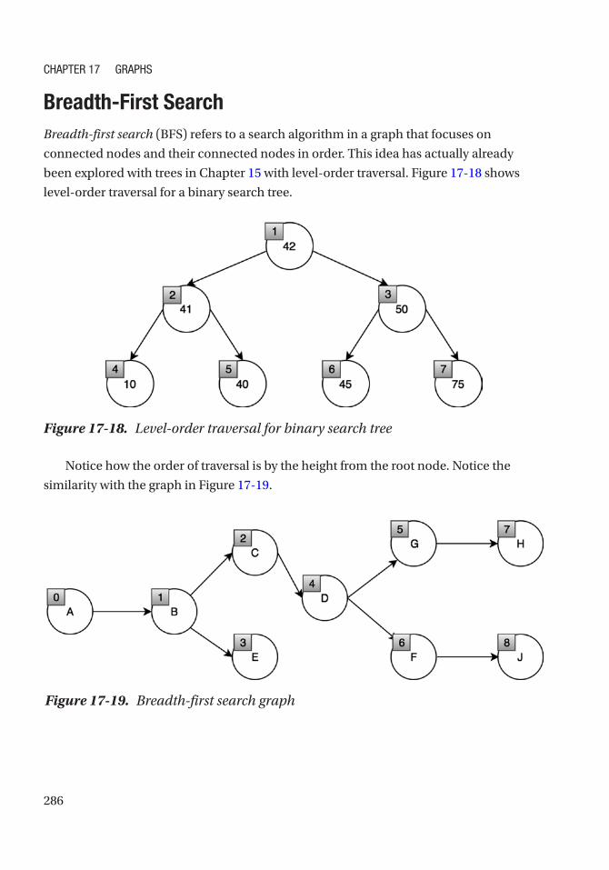
286
Breadth-First SearchBreadth-first search (BFS) refers to a search algorithm in a graph that focuses on
connected nodes and their connected nodes in order. This idea has actually already
been explored with trees in Chapter 15 with level-order traversal. Figure 17-18 shows
level-order traversal for a binary search tree.
Figure 17-18. Level-order traversal for binary search tree
Notice how the order of traversal is by the height from the root node. Notice the
similarity with the graph in Figure 17-19.
Figure 17-19. Breadth-first search graph
ChaPTeR 17 GRaPhS
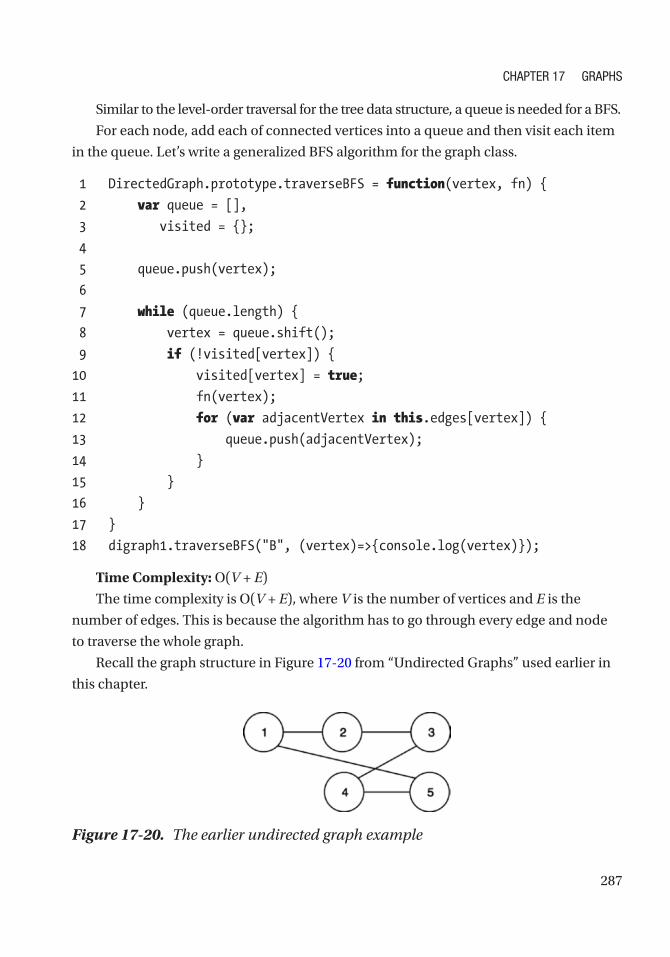
287
Similar to the level-order traversal for the tree data structure, a queue is needed for a BFS.
For each node, add each of connected vertices into a queue and then visit each item
in the queue. Let’s write a generalized BFS algorithm for the graph class.
1 DirectedGraph.prototype.traverseBFS = function(vertex, fn) {
2 var queue = [],
3 visited = {};
4
5 queue.push(vertex);
6
7 while (queue.length) {
8 vertex = queue.shift();
9 if (!visited[vertex]) {
10 visited[vertex] = true;
11 fn(vertex);
12 for (var adjacentVertex in this.edges[vertex]) {
13 queue.push(adjacentVertex);
14 }
15 }
16 }
17 }
18 digraph1.traverseBFS("B", (vertex)=>{console.log(vertex)});
Time Complexity: O(V + E)
The time complexity is O(V + E), where V is the number of vertices and E is the
number of edges. This is because the algorithm has to go through every edge and node
to traverse the whole graph.
Recall the graph structure in Figure 17-20 from “Undirected Graphs” used earlier in
this chapter.
Figure 17-20. The earlier undirected graph example
ChaPTeR 17 GRaPhS

288
Applying the BFS to the graph, the following is printed: 1, 2, 5, 3, 4.
In Figures 17-21 and 17-22, the lightly shaded node represents the node being
currently visited, while the dark node represents that the node has already been visited.
Figure 17-21. Breadth-first search, part 1
In Figure 17-21, the breadth-first search starts at the 1 node. Because it has two
neighbors, 2 and 5, those are added to the queue. Then, 2 is visited, and its neighbor
3 is added to the queue. 5 is then dequeued, and its neighbor 4 is added to the queue.
Finally, 3 and 4 are visited, and the search ends, as shown in Figure 17-22.
ChaPTeR 17 GRaPhS

289
Depth-First SearchDepth-first search (DFS) refers to a search algorithm in a graph that focuses on traversing
deep into one connection before visiting the other connections.
This idea has been explored in Chapter 15 with in-order, post-order, and pre-order
traversals in trees. For example, a post-order tree traversal visits the bottom children
node before visiting the top root nodes (see Figure 17-23).
Figure 17-22. Breadth-first search, part 2
ChaPTeR 17 GRaPhS
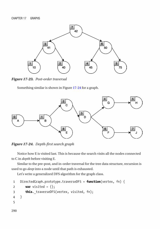
290
Something similar is shown in Figure 17-24 for a graph.
Figure 17-23. Post-order traversal
Figure 17-24. Depth-first search graph
Notice how E is visited last. This is because the search visits all the nodes connected
to C in depth before visiting E.
Similar to the pre-post, and in-order traversal for the tree data structure, recursion is
used to go deep into a node until that path is exhausted.
Let’s write a generalized DFS algorithm for the graph class.
1 DirectedGraph.prototype.traverseDFS = function(vertex, fn) {
2 var visited = {};
3 this._traverseDFS(vertex, visited, fn);
4 }
5
ChaPTeR 17 GRaPhS

291
6 DirectedGraph.prototype._traverseDFS = function(vertex, visited, fn) {
7 visited[vertex] = true;
8 fn(vertex);
9 for (var adjacentVertex in this.edges[vertex]) {
10 if (!visited[adjacentVertex]) {
11 this._traverseDFS(adjacentVertex, visited, fn);
12 }
13 }
14 }
Time Complexity: O(V + E)
The time complexity is O(V + E) where V is the number of vertices and E is the
number of edges. This is because the algorithm has to go through every edge and node
to traverse the whole graph. This is the same time complexity as the BFS algorithm.
Again, let’s use the graph structure from earlier in the chapter (see Figure 17-25).
Figure 17-25. The earlier graph example from Figure 17-20
Applying the DFS to the graph, the following is printed: 1, 2, 3, 4, 5.
In Figures 17-26 and 17-27, the lightly shaded node represents the node being
currently visited, while the dark node represents that the node has already been visited.
ChaPTeR 17 GRaPhS

292
In Figure 17-26, the depth-first search starts at the 1 node. Its first neighbor, 2,
is visited. Then, 2’s first neighbor, 3, is visited. After 3 is visited, 4 will be visited next
because it is 3’s first neighbor. Finally, 4 is visited followed by 5, as shown in Figure 17-27.
Depth-first search always visits the first neighbor recursively.
Figure 17-26. Depth-first search, part 1
ChaPTeR 17 GRaPhS

293
Weighted Graphs and Shortest PathNow that we have covered the basics of graphs and how to traverse them, we can discuss
weighted edges and Dijkstra’s algorithm, which employs shortest path searches.
Graphs with Weighted EdgesRecall that edges in a graph represent a connection between the vertices. If edges
establish a connection, weight can be assigned to that connection. For example, for a
graph that represents a map, the weights on the edges are distances.
It is important to note that the graphical length of an edge means nothing with
regard to the edge’s weight. It is purely there for visual purposes. In the implementation
and the code, the visual representation is not required. In Figure 17-28, the weights tell
us the distances between the cities in a graph representation of five cities. For example,
graphically, the distance from City 1 and City 2 is shorter than the distance from City 2
and City 3. However, the edges indicate that the distance from City 1 to City 2 is 50 km,
and the distance from City 2 to City 3 is 10 km, which is five times larger.
Figure 17-27. Depth-first search, part 2
ChaPTeR 17 GRaPhS

294
Figure 17-28. Graph representation of five cities
The most important question for weighted edge graphs is, what is the shortest path
from one node to another? There are series of shortest path algorithms for graphs. The
one we discuss is Dijkstra’s algorithm.
Dijkstra’s Algorithm: Shortest PathDijkstra’s algorithm works by taking the shortest path at each level to get to a destination.
At first, the distance is marked as infinity because some nodes may not be reachable (see
Figure 17-29). Then at each traversal iteration, the shortest distance is chosen for each
node (see Figures 17-30 and 17-31).
Figure 17-29. Dijkstra stage 1: everything marked as infinity
ChaPTeR 17 GRaPhS

295
Figure 17-30. Dijkstra stage 2: B and C processed
Figure 17-31. Dijkstra stage 3: all nodes now processed
_extractMin is implemented to compute the neighboring node with the smallest
distance for a given vertex. Using the breadth-first search outline to enqueue the
neighboring nodes for each vertex as the graph is traversed from the origin to the
destination node, the distances are updated and computed.
1 function _isEmpty(obj) {
2 return Object.keys(obj).length === 0;
3 }
4
5 function _extractMin(Q, dist) {
6 var minimumDistance = Infinity,
7 nodeWithMinimumDistance = null;
8 for (var node in Q) {
9 if (dist[node] <= minimumDistance) {
10 minimumDistance = dist[node];
ChaPTeR 17 GRaPhS

296
11 nodeWithMinimumDistance = node;
12 }
13 }
14 return nodeWithMinimumDistance;
15 }
16
17 DirectedGraph.prototype.Dijkstra = function(source) {
18 // create vertex set Q
19 var Q = {}, dist = {};
20 for (var vertex in this.edges) {
21 // unknown distances set to Infinity
22 dist[vertex] = Infinity;
23 // add v to Q
24 Q[vertex] = this.edges[vertex];
25 }
26 // Distance from source to source init to 0
27 dist[source] = 0;
28
29 while (!_isEmpty(Q)) {
30 var u = _extractMin(Q, dist); // get the min distance
31
32 // remove u from Q
33 delete Q[u];
34
35 // for each neighbor, v, of u:
36 // where v is still in Q.
37 for (var neighbor in this.edges[u]) {
38 // current distance
39 var alt = dist[u] + this.edges[u][neighbor];
40 // a shorter path has been found
41 if (alt < dist[neighbor]) {
42 dist[neighbor] = alt;
43 }
44 }
45 }
ChaPTeR 17 GRaPhS

297
46 return dist;
47 }
48
49 var digraph1 = new DirectedGraph();
50 digraph1.addVertex("A");
51 digraph1.addVertex("B");
52 digraph1.addVertex("C");
53 digraph1.addVertex("D");
54 digraph1.addEdge("A", "B", 1);
55 digraph1.addEdge("B", "C", 1);
56 digraph1.addEdge("C", "A", 1);
57 digraph1.addEdge("A", "D", 1);
58 console.log(digraph1);
59 // DirectedGraph {
60 // V: 4,
61 // E: 4,
62 // edges: { A: { B: 1, D: 1 }, B: { C: 1 }, C: { A: 1 }, D: {} }}
63 digraph1.Dijkstra("A"); // { A: 0, B: 1, C: 2, D: 1 }
Time Complexity: O(V 2 + E)
The algorithm here is similar to the BFS algorithm but requires the _extractMin
method, which is O(n) in time complexity. Because of this, the time complexity is
O(V 2 + E) because all neighbor vertices of the node currently being traversed have to
be checked during the _extractMin method. This algorithm can be improved using a
priority queue for the extract min, which would yield O(log2(V )) _extractMin and hence
yield an overall time complexity of O(E + V) * O(log2(V)) = O(E log2(V)). This can be
even more optimized by using a Fibonacci heap, which has constant time to compute
_extractMin. However, for simplicity, neither a Fibonacci heap nor a priority queue was
used for this demonstration.
ChaPTeR 17 GRaPhS

298
Topological SortFor a directed graph, it can be important to know which node should be processed first
for various applications. An example of this is a task scheduler where one task depends
on a previous task being done. Another example is a JavaScript library dependency
manager where it has to figure out which libraries to import before others. The
topological sorting algorithm implements this. It is a modified DFS that uses a stack to
record the order.
Put simply, it works by performing DFS from a node until its connected nodes are
recursively exhausted and by adding it to the stack until the connected nodes are all
visited (see Figure 17-32).
Figure 17-32. Topological sort
ChaPTeR 17 GRaPhS

299
Topological sorting has a visited set to ensure that the recursive call does not result in
an infinite loop. For a given node, that node is added to the visited set, and its neighbors
that have not been visited are visited in the next recursive call. At the end of the recursive
call, unshift is used to add the current node’s value to the stack. This ensures that the
order is chronological.
1 DirectedGraph.prototype.topologicalSortUtil = function(v, visited, stack) {
2 visited.add(v);
3
4 for (var item in this.edges[v]) {
5 if (visited.has(item) == false) {
6 this.topologicalSortUtil(item, visited, stack)
7 }
8 }
9 stack.unshift(v);
10 };
11
12 DirectedGraph.prototype.topologicalSort = function() {
13 var visited = {},
14 stack = [];
15
16
17 for (var item in this.edges) {
18 if (visited.has(item) == false) {
19 this.topologicalSortUtil(item, visited, stack);
20 }
21 }
22 return stack;
23 };
24
25 var g = new DirectedGraph();
26 g.addVertex('A');
27 g.addVertex('B');
28 g.addVertex('C');
29 g.addVertex('D');
30 g.addVertex('E');
ChaPTeR 17 GRaPhS

300
31 g.addVertex('F');
32
33 g.addEdge('B', 'A');
34 g.addEdge('D', 'C');
35 g.addEdge('D', 'B');
36 g.addEdge('B', 'A');
37 g.addEdge('A', 'F');
38 g.addEdge('E', 'C');
39 var topologicalOrder = g.topologicalSort();
40 console.log(g);
41 // DirectedGraph {
42 // V: 6,
43 // E: 6,
44 // edges:
45 // { A: { F: 0 },
46 // B: { A: 0 },
47 // C: {},
48 // D: { C: 0, B: 0 },
49 // E: { C: 0 },
50 // F: {} } }
51 console.log(topologicalOrder); // [ 'E', 'D', 'C', 'B', 'A', 'F' ]
Time Complexity: O(V + E)
Space Complexity: O(V)
The topological sort algorithm is simply DFS with an extra stack. Therefore, the time
complexity is the same as DFS. Topological sorting requires O(V) in space because it
needs to store all the vertices in the stack. This algorithm is powerful for scheduling jobs
from given dependencies.
SummaryThis chapter discussed different types of graphs, their properties, and how to search
and sort them. A graph, composed of vertices and connected via edges, can be
represented as a data structure in many different ways. In this chapter, an adjacency list
was used to represent the graph. If the graph is dense, it is better to use a matrix-based
ChaPTeR 17 GRaPhS
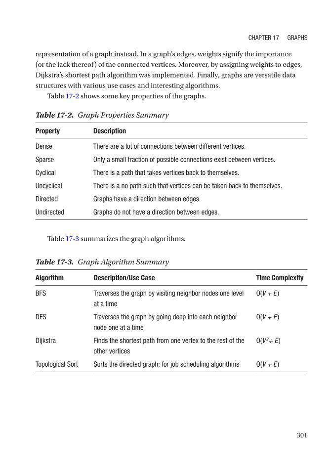
301
representation of a graph instead. In a graph’s edges, weights signify the importance
(or the lack thereof) of the connected vertices. Moreover, by assigning weights to edges,
Dijkstra’s shortest path algorithm was implemented. Finally, graphs are versatile data
structures with various use cases and interesting algorithms.
Table 17-2 shows some key properties of the graphs.
Table 17-3. Graph Algorithm Summary
Algorithm Description/Use Case Time Complexity
BFS Traverses the graph by visiting neighbor nodes one level
at a time
O(V + E )
DFS Traverses the graph by going deep into each neighbor
node one at a time
O(V + E )
Dijkstra Finds the shortest path from one vertex to the rest of the
other vertices
O(V 2+ E )
Topological Sort Sorts the directed graph; for job scheduling algorithms O(V + E )
Table 17-2. Graph Properties Summary
Property Description
Dense There are a lot of connections between different vertices.
Sparse Only a small fraction of possible connections exist between vertices.
Cyclical There is a path that takes vertices back to themselves.
Uncyclical There is a no path such that vertices can be taken back to themselves.
Directed Graphs have a direction between edges.
Undirected Graphs do not have a direction between edges.
Table 17-3 summarizes the graph algorithms.
ChaPTeR 17 GRaPhS

303© Sammie Bae 2019 S. Bae, JavaScript Data Structures and Algorithms, https://doi.org/10.1007/978-1-4842-3988-9_18
CHAPTER 18
Advanced StringsThis chapter will cover more advanced string algorithms than the previous chapters have
discussed. They should be easier to understand now that you have learned about some
other data structures. Specifically, this chapter will focus on string searching algorithms.
Trie (Prefix Tree)A trie is special type of tree used commonly for searching strings and matching on
stored strings. At each level, nodes can branch off to form complete words. For example,
Figure 18-1 shows a trie of the words: Sammie, Simran, Sia, Sam. Each ending node has
a boolean flag: isCompleted. This indicates that the word ends in this path. For example,
m in Sam has endOfWord set to true. Nodes with endOfWord set to true are shaded in
Figure 18-1.

304
A trie is implemented using a nested object where each level has its direct children
as keys. A trie node can be formed by using an object to store the children. The trie
has a root node that is instantiated in the constructor of the Trie class, as shown in the
following code block:
1 function TrieNode() {
2 this.children = {}; // table
3 this.endOfWord = false;
4 }
5
6 function Trie() {
7 this.root = new TrieNode();
8 }
Figure 18-1. Trie of Sammie, Simran, Sia, Sam
Chapter 18 advanCed StringS
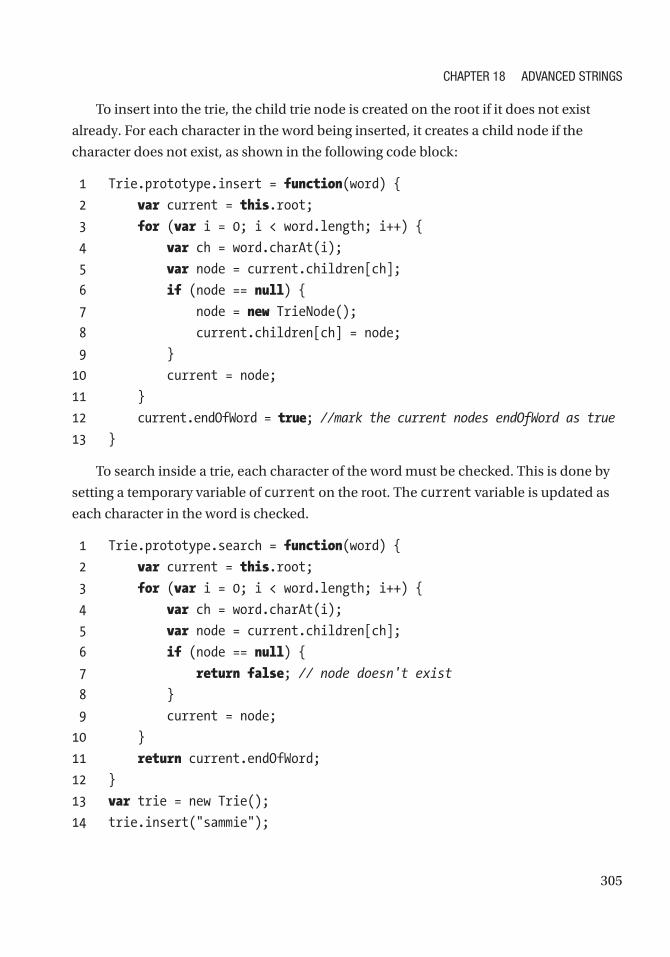
305
To insert into the trie, the child trie node is created on the root if it does not exist
already. For each character in the word being inserted, it creates a child node if the
character does not exist, as shown in the following code block:
1 Trie.prototype.insert = function(word) {
2 var current = this.root;
3 for (var i = 0; i < word.length; i++) {
4 var ch = word.charAt(i);
5 var node = current.children[ch];
6 if (node == null) {
7 node = new TrieNode();
8 current.children[ch] = node;
9 }
10 current = node;
11 }
12 current.endOfWord = true; //mark the current nodes endOfWord as true
13 }
To search inside a trie, each character of the word must be checked. This is done by
setting a temporary variable of current on the root. The current variable is updated as
each character in the word is checked.
1 Trie.prototype.search = function(word) {
2 var current = this.root;
3 for (var i = 0; i < word.length; i++) {
4 var ch = word.charAt(i);
5 var node = current.children[ch];
6 if (node == null) {
7 return false; // node doesn't exist
8 }
9 current = node;
10 }
11 return current.endOfWord;
12 }
13 var trie = new Trie();
14 trie.insert("sammie");
Chapter 18 advanCed StringS

306
15 trie.insert("simran");
16 trie.search("simran"); // true
17 trie.search("fake") // false
18 trie.search("sam") // false
To delete an element from a trie, the algorithm should traverse the root node until it
reaches the last character of the word. Then, for each node that does not have any other
children, the node should be deleted. For example, in a trie with sam and sim, when
sim is deleted, the s node in the root stays intact, but i and m are removed. The recursive
implementation in the following code block implements this algorithm:
1 Trie.prototype.delete = function(word) {
2 this.deleteRecursively(this.root, word, 0);
3 }
4
5 Trie.prototype.deleteRecursively = function(current, word, index) {
6 if (index == word.length) {
7 //when end of word is reached only delete if currrent.end Of
Word is true.
8 if (!current.endOfWord) {
9 return false;
10 }
11 current.endOfWord = false;
12 //if current has no other mapping then return true
13 return Object.keys(current.children).length == 0;
14 }
15 var ch = word.charAt(index),
16 node = current.children[ch];
17 if (node == null) {
18 return false;
19 }
20 var shouldDeleteCurrentNode = this.deleteRecursively(node, word,
index + 1);
21
22 // if true is returned then
23 // delete the mapping of character and trienode reference from map.
Chapter 18 advanCed StringS
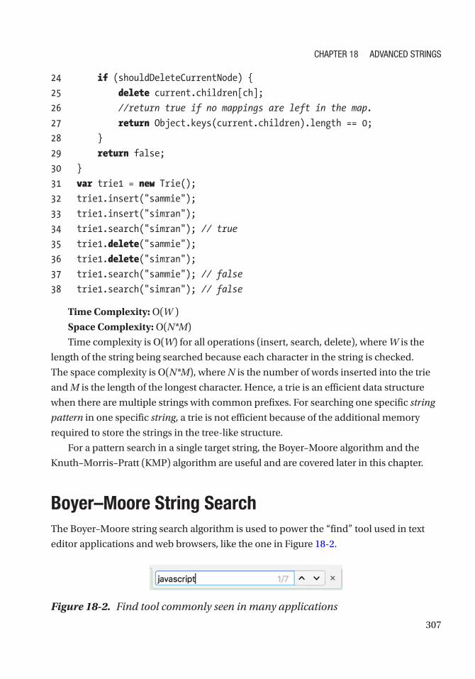
307
24 if (shouldDeleteCurrentNode) {
25 delete current.children[ch];
26 //return true if no mappings are left in the map.
27 return Object.keys(current.children).length == 0;
28 }
29 return false;
30 }
31 var trie1 = new Trie();
32 trie1.insert("sammie");
33 trie1.insert("simran");
34 trie1.search("simran"); // true
35 trie1.delete("sammie");
36 trie1.delete("simran");
37 trie1.search("sammie"); // false
38 trie1.search("simran"); // false
Time Complexity: O(W )
Space Complexity: O(N*M)
Time complexity is O(W) for all operations (insert, search, delete), where W is the
length of the string being searched because each character in the string is checked.
The space complexity is O(N*M), where N is the number of words inserted into the trie
and M is the length of the longest character. Hence, a trie is an efficient data structure
when there are multiple strings with common prefixes. For searching one specific string
pattern in one specific string, a trie is not efficient because of the additional memory
required to store the strings in the tree-like structure.
For a pattern search in a single target string, the Boyer–Moore algorithm and the
Knuth–Morris–Pratt (KMP) algorithm are useful and are covered later in this chapter.
Boyer–Moore String SearchThe Boyer–Moore string search algorithm is used to power the “find” tool used in text
editor applications and web browsers, like the one in Figure 18-2.
Figure 18-2. Find tool commonly seen in many applications
Chapter 18 advanCed StringS
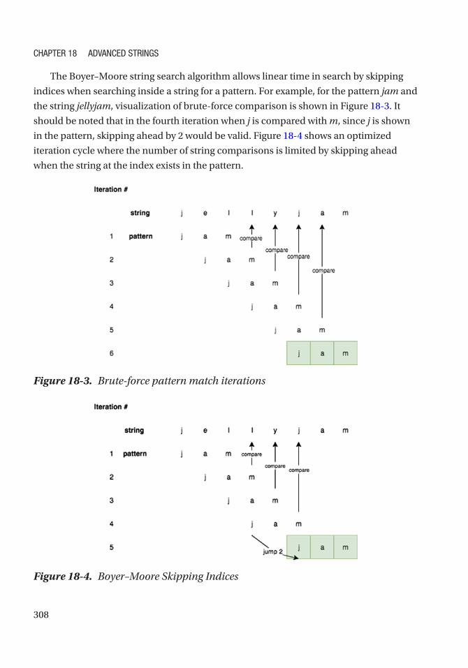
308
The Boyer–Moore string search algorithm allows linear time in search by skipping
indices when searching inside a string for a pattern. For example, for the pattern jam and
the string jellyjam, visualization of brute-force comparison is shown in Figure 18-3. It
should be noted that in the fourth iteration when j is compared with m, since j is shown
in the pattern, skipping ahead by 2 would be valid. Figure 18-4 shows an optimized
iteration cycle where the number of string comparisons is limited by skipping ahead
when the string at the index exists in the pattern.
Figure 18-3. Brute-force pattern match iterations
Figure 18-4. Boyer–Moore Skipping Indices
Chapter 18 advanCed StringS

309
To implement this skip rule, you can build a “bad match table” structure. The
bad match table indicates how much to skip for a given character of a pattern. Some
examples of various patterns and its corresponding bad match table are shown here:
Pattern Bad Match Table
jam {j: 2, a: 1, m: 3}
data {d: 3, a: 2, t: 1}
struct {s: 5, t: 4, r: 3, u: 2, c: 1}
roi {r: 2, o: 1, i: 3}
For the roi example, r:2 indicates that if r is not found in the string, the index should
skip by 2. This bad match table can be implemented with the following code block:
function buildBadMatchTable(str) {
var tableObj = {},
strLength = str.length;
for (var i = 0; i < strLength - 1; i++) {
tableObj[str[i]] = strLength - 1 - i;
}
if (tableObj[str[strLength-1]] == undefined) {
tableObj[str[strLength-1]] = strLength;
}
return tableObj;
}
buildBadMatchTable('data'); // {d: 3, a: 2, t: 1}
buildBadMatchTable('struct'); // {s: 5, t: 4, r: 3, u: 2, c: 1}
buildBadMatchTable('roi'); // {r: 2, o: 1, i: 3}
buildBadMatchTable('jam'); // {j: 2, a: 1, m: 3}
Using this bad match table, the Boyer–Moore string search algorithm can be
implemented. When scanning the input string for the pattern, if the current string
being looked at exists in the bad match table, it skips over by the bad match table value
associated with the current string. Otherwise, it is incremented by 1. This continues until
Chapter 18 advanCed StringS
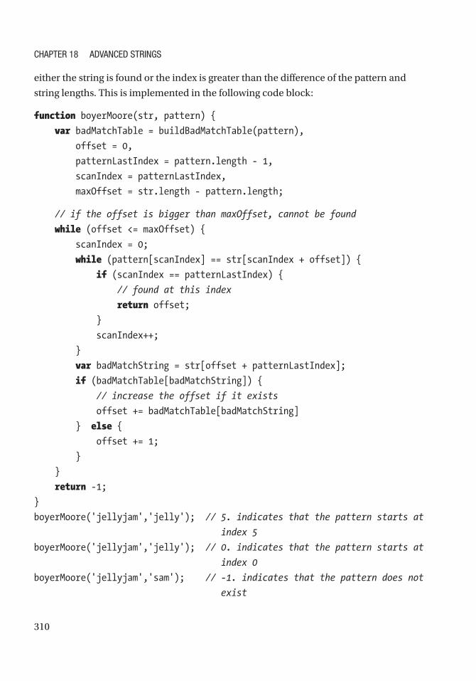
310
either the string is found or the index is greater than the difference of the pattern and
string lengths. This is implemented in the following code block:
function boyerMoore(str, pattern) {
var badMatchTable = buildBadMatchTable(pattern),
offset = 0,
patternLastIndex = pattern.length - 1,
scanIndex = patternLastIndex,
maxOffset = str.length - pattern.length;
// if the offset is bigger than maxOffset, cannot be found
while (offset <= maxOffset) {
scanIndex = 0;
while (pattern[scanIndex] == str[scanIndex + offset]) {
if (scanIndex == patternLastIndex) {
// found at this index
return offset;
}
scanIndex++;
}
var badMatchString = str[offset + patternLastIndex];
if (badMatchTable[badMatchString]) {
// increase the offset if it exists
offset += badMatchTable[badMatchString]
} else {
offset += 1;
}
}
return -1;
}
boyerMoore('jellyjam','jelly'); // 5. indicates that the pattern starts at
index 5
boyerMoore('jellyjam','jelly'); // 0. indicates that the pattern starts at
index 0
boyerMoore('jellyjam','sam'); // -1. indicates that the pattern does not
exist
Chapter 18 advanCed StringS
311
Best Case:In the best case, all the characters in the pattern are the same, and this consistently
produces shifts by T, where T is the length of the pattern. Hence, O(W/T) is the best
time complexity where W is the string where the pattern is being searched. The space
complexity is O(1) since only 1 value is stored into the bad match table.
Time Complexity: O(T/W)
Space Complexity: O(1)
Worst Case:In the worst case, the string has the pattern at the end of the string, and the
preceding part is all unique characters. An example of this is a string of abcdefgxyz and
pattern of xyz. In this case, T*W string comparisons are done.
Time Complexity: O(T*W)
Space Complexity: O(T)
All the characters in the pattern and the string are the same. An example of such a
case is the string bbbbbb and the pattern bbb. This case cannot use the skip mechanism
to its fullest because the index will always be incremented by 1. Space complexity in this
case is T because the pattern could have all unique characters.
Knuth–Morris–Pratt String SearchChapter 4 discussed the native String.prototype.indexOf function. A naive
implementation of the String.prototype.indexOf function was included as an exercise
for that chapter. A better (faster) implementation uses the Knuth–Morris–Pratt (KMP)
string search algorithm. The following implementation of the KMP algorithm returns all
indices where the pattern is present.
The KMP string searching algorithm searches for occurrences of the “word” W
within an input “text,” which is T, by utilizing the observation that the occurrence of a
mismatch contains sufficient information about where the next match could begin. This
helps to skip re-examination of previously matched characters. A prefix array has to be
Chapter 18 advanCed StringS

312
built to indicate how many indices it has to backtrack to get the same prefix. For the
string ababaca, the prefix building looks like the following:
At current index 0, there is no string to compare to, and the prefix array value is
initialized to 0.
array index 0 1 2 3 4 5 6
character a b a b a c a
prefix array 0
At current index 1:
• The character is b.
• The previous prefix array value, prefix[0], is 0.
Compare index 0 to the current index: a (at index = 0) and b (at index = 1) mismatch.
prefix[1] is set to 0:
Array index 0 1 2 3 4 5 6
Character a b a b a c a
Prefix array 0 0
At current index 2:
• The character is a.
• The previous prefix array value, prefix[1], is 0.
Compare the index and to the current index: a (at index = 0) and a (at index = 2)
match.
prefix[2] is set to 1 (incremented from prefix[1]):
Array index 0 1 2 3 4 5 6
Character a b a b a c a
Prefix array 0 0 1
At current index 3:
• The character is b.
• The previous prefix array value, prefix[2], is 1.
Chapter 18 advanCed StringS
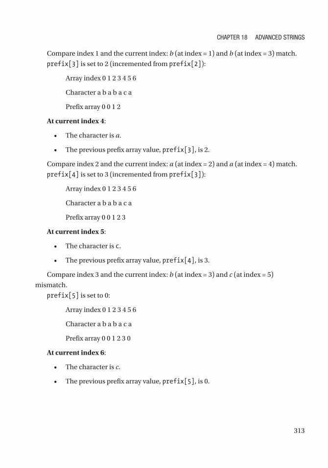
313
Compare index 1 and the current index: b (at index = 1) and b (at index = 3) match.
prefix[3] is set to 2 (incremented from prefix[2]):
Array index 0 1 2 3 4 5 6
Character a b a b a c a
Prefix array 0 0 1 2
At current index 4:
• The character is a.
• The previous prefix array value, prefix[3], is 2.
Compare index 2 and the current index: a (at index = 2) and a (at index = 4) match.
prefix[4] is set to 3 (incremented from prefix[3]):
Array index 0 1 2 3 4 5 6
Character a b a b a c a
Prefix array 0 0 1 2 3
At current index 5:
• The character is c.
• The previous prefix array value, prefix[4], is 3.
Compare index 3 and the current index: b (at index = 3) and c (at index = 5)
mismatch.
prefix[5] is set to 0:
Array index 0 1 2 3 4 5 6
Character a b a b a c a
Prefix array 0 0 1 2 3 0
At current index 6:
• The character is c.
• The previous prefix array value, prefix[5], is 0.
Chapter 18 advanCed StringS

314
Compare from index 0 and current index: a (at index = 0) and a (at index = 5) match.
prefix[6] is set to 1 (incremented from prefix[5]):
Array index 0 1 2 3 4 5 6
Character a b a b a c a
Prefix array 0 0 1 2 3 0 1
The function in the following code block illustrates this algorithm to build a prefix
table:
function longestPrefix(str) {
// prefix array is created
var prefix = new Array(str.length);
var maxPrefix = 0;
// start the prefix at 0
prefix[0] = 0;
for (var i = 1; i < str.length; i++) {
// decrement the prefix value as long as there are mismatches
while (str.charAt(i) !== str.charAt(maxPrefix) && maxPrefix > 0) {
maxPrefix = prefix[maxPrefix - 1];
}
// strings match, can update it
if (str.charAt(maxPrefix) === str.charAt(i)) {
maxPrefix++;
}
// set the prefix
prefix[i] = maxPrefix;
}
return prefix;
}
console.log(longestPrefix('ababaca')); // [0, 0, 1, 2, 3, 0, 1]
With this prefix table now, KMP can be implemented. KMP search iterates
through the string and the pattern to be searched for index by index. Whenever there
is a mismatch, it can use the prefix table to compute a new index to try.
Chapter 18 advanCed StringS

315
When the pattern’s index reaches the length of the pattern, the string is found. This is
implemented in detail in the following code block:
function KMP(str, pattern) {
// build the prefix table
var prefixTable = longestPrefix(pattern),
patternIndex = 0,
strIndex = 0;
while (strIndex < str.length) {
if (str.charAt(strIndex) != pattern.charAt(patternIndex)) {
// Case 1: the characters are different
if (patternIndex != 0) {
// use the prefix table if possible
patternIndex = prefixTable[patternIndex - 1];
} else {
// increment the str index to next character
strIndex++;
}
} else if (str.charAt(strIndex) == pattern.charAt(patternIndex)) {
// Case 2: the characters are same
strIndex++;
patternIndex++;
}
// found the pattern
if (patternIndex == pattern.length) {
return true
}
}
return false;
}
KMP('ababacaababacaababacaababaca', 'ababaca'); // true
KMP('sammiebae', 'bae'); // true
KMP('sammiebae', 'sammie'); // true
KMP('sammiebae', 'sammiebaee'); // false
Chapter 18 advanCed StringS

316
Time Complexity: O(W)
Space Complexity: O(W )
Preprocessing a word of length W requires both O(W) time and space complexity.
Time Complexity: O(W + T )
Here, W is the “word” in the T (the main string being searched).
Rabin–Karp SearchThe Rabin–Karp algorithm is based on hashing to find the specified pattern in text.
While KMP is optimized to skip redundant checks during the search, Rabin–Karp seeks
to speed up the equality of the pattern of the substring via a hash function. To do this
efficiently, the hash function must be O(1). Specifically for the Rabin-Karp search, the
Rabin fingerprint hashing technique is used.
The Rabin FingerprintThe Rabin fingerprint is calculated via the following equation: f(x) = m0 + m1x + … + mn-1
xn-1 where n is the number of characters being hashed and x is some prime number.
This is a simple implementation, as shown in the following code block. An arbitrary
prime number of 101 was set for this example. Any high prime number should work well
in this case. However, be aware that if the x is too high, it could cause integer overflow
because xn-1 grows quickly. The endLength argument indicates to what string index the
hash should be calculated. It should be defaulted to the length of str if the argument is
not passed.
1 function RabinKarpSearch() {
2 this.prime = 101;
3 }
4 RabinKarpSearch.prototype.rabinkarpFingerprintHash = function (str,
endLength) {
5 if (endLength == null) endLength = str.length;
6 var hashInt = 0;
7 for (var i=0; i < endLength; i++) {
8 hashInt += str.charCodeAt(i) * Math.pow(this.prime, i);
9 }
10 return hashInt;
Chapter 18 advanCed StringS

317
11 }
12 var rks = new RabinKarpSearch();
13 rks.rabinkarpFingerprintHash("sammie"); // 1072559917336
14 rks.rabinkarpFingerprintHash("zammie"); // 1072559917343
As shown in the previous code block result, the hashes from sammie and zammie are
unique because they are two different strings. The hash value allows you to quickly, in
constant time, check whether two strings are the same. As an example, let’s look for am
inside same. Since am is only two characters long, when you scan the text, sa, am, and
me are formed from same and compute the hash as shown here:
1 rks.rabinkarpFingerprintHash("sa"); // 9912
2 rks.rabinkarpFingerprintHash("am"); // 11106
3 rks.rabinkarpFingerprintHash("me"); // 10310
This is a sliding hash calculation. How can this be done efficiently? Let’s analyze it
mathematically. Recall that for this example the x is 101. In addition, the character code
for s, a, m, and e are 115, 97, 109, and 101, respectively.
sa: f(x) = m0 + m1x = 115 + (97)*(101) = 9912
am: f(x) = m0 + m1x = 97 + (109)*(101) = 11106
me: f(x) = m0 + m1x = 109 + (101)*(101) = 10310
To get the hash value from sa to am, you must subtract the first term, divide the
remaining by the prime number, and then add the new term. This recalculation
algorithm is implemented in the following code block:
1 RabinKarpSearch.prototype.recalculateHash = function (str, oldIndex,
newIndex, oldHash, patternLength) {
2 if (patternLength == null) patternLength = str.length;
3 var newHash = oldHash - str.charCodeAt(oldIndex);
4 newHash = Math.floor(newHash/this.prime);
5 newHash += str.charCodeAt(newIndex) * Math.pow(this.prime,
patternLength - 1);
6 return newHash;
7 }
8 var oldHash = rks.rabinkarpFingerprintHash("sa"); // 9912
9 rks.recalculateHash("same", 0, 2, oldHash, "sa".length); // 11106
Chapter 18 advanCed StringS

318
Lastly, two different strings can still have the same hash value although it’s unlikely.
Therefore, there needs to be a function to check that two strings are equal given the start
index and end index for both strings. This is implemented in the following code block:
1 RabinKarpSearch.prototype.strEquals = function ( str1, startIndex1,
endIndex1,
2 str2, startIndex2,
endIndex2) {
3 if (endIndex1 - startIndex1 != endIndex2 - startIndex2) {
4 return false;
5 }
6 while ( startIndex1 <= endIndex1
7 && startIndex2 <= endIndex2) {
8 if (str1[startIndex1] != str2[startIndex2]) {
9 return false;
10 }
11 startIndex1++;
12 startIndex2++;
13 }
14 return true;
15 }
Then, the main Rabin–Karp search function is implemented by calculating the
starting hash and then recalculating the hashes in a sliding manner until the pattern is
found or the end of the string is reached.
1 RabinKarpSearch.prototype.rabinkarpSearch = function (str, pattern) {
2 var T = str.length,
3 W = pattern.length,
4 patternHash = this.rabinkarpFingerprintHash(pattern, W),
5 textHash = this.rabinkarpFingerprintHash(str, W);
6
7 for (var i = 1; i <= T - W + 1; i++) {
8 if (patternHash == textHash &&
9 this.strEquals(str, i - 1, i + W - 2, pattern, 0, W - 1)) {
10 return i - 1;
11 }
Chapter 18 advanCed StringS

319
12 if (i < T - W + 1) {
13 textHash = this.recalculateHash(str, i - 1, i + W - 1,
textHash, W);
14 }
15 }
16
17 return -1;
18 }
19
20 var rks = new RabinKarpSearch();
21 rks.rabinkarpSearch("SammieBae", "as"); // -1
22 rks.rabinkarpSearch("SammieBae", "Bae"); // 6
23 rks.rabinkarpSearch("SammieBae", "Sam"); // 0
Preprocessing Time Complexity: O(W )
The preprocessing time complexity W is the length of the “word.”
Matching Time Complexity: O(W + T )
At most, this algorithm iterates through the sum of length T and length W, where T is
the string being searched for.
Applications in Real LifeThe Rabin–Karp algorithm can be used for detecting plagiarism. With a source material,
this algorithm can search through a paper submission for instances of phrases and
sentences from the source material (and ignoring grammar details like punctuation
by omitting punctuation characters during the preprocessing phase). This problem
is impractical for single-search algorithms because of the large set of sought (input)
phrases and sentences. The Rabin–Karp algorithm is also used in other string matching
applications such as looking for a specific sequence in large DNA data.
Chapter 18 advanCed StringS

320
SummaryThis chapter returned to the topic of strings and looked at more advanced examples and
searching on string patterns. The chapter discussed several different types.
• Trie is great for multiple searches and prefix pattern matching.
• Boyer–Moore, with assumption that the absence of a match at the
end means no need to match the beginning, tries to match the last
character of the pattern instead of the first; this allows large “jumps”
(spaces between indexes) and works better when the text is larger.
• The KMP algorithm searches for occurrences of the pattern in a
string by observing that when a mismatch occurs, the pattern itself
has sufficient information to determine the index in the string where
the next match could begin. Hence, the KMP algorithm is better for
small sets.
Table 18-1 summarizes the different search algorithms.
Table 18-1. Single String Search Summary
Algorithm Preprocessing Time Complexity
Matching Time Complexity
Space Complexity
naive none O(W ∗ T ) none
Boyer–Moore O(W + T ) O(T /W ) best case
O(W ∗ T ) worst case
O(1)
KMp O(W ) O(T ) O(W )
rabin–Karp O(W ) O(W + T ) O(1)
Chapter 18 advanCed StringS

321© Sammie Bae 2019 S. Bae, JavaScript Data Structures and Algorithms, https://doi.org/10.1007/978-1-4842-3988-9_19
CHAPTER 19
Dynamic ProgrammingDynamic programming involves breaking down problems into their subproblems.
By solving for the optimal subproblems and saving those results into memory to access
them whenever a repeated problem needs to be solved, the algorithmic complexity
decreases significantly. Implementing dynamic programming algorithms requires
higher-level thinking about the problem’s patterns. To explain dynamic programming,
let’s re-examine the Fibonacci sequence that was discussed in Chapter 8. Then the
chapter will cover the rules of dynamic programming and walk you through some
examples to make the concepts more concrete.
Motivations for Dynamic ProgrammingThe code for the Fibonacci sequence has already been determined to be the following:
function getNthFibo(n) {
if (n <= 1) {
return n;
} else {
return getNthFibo(n - 1) + getNthFibo(n - 2);
}
}
getNthFibo(3);
Recall that the recursive implementation of this algorithm is O(2n). This is an
exponential runtime, which is impractical for real-world applications. Upon closer
examination, you will notice that much of the same computation is repeated. As shown
in Figure 19-1, when getNthFibo for 6 is called, the calculation for 4, 3, 2, and 1 are
repeated multiple times. Knowing this, how can you make this algorithm more efficient?

322
Using a hash table, once the Fibonacci number has been computed, it can be stored
like the following implementation:
1 var cache={};
2 function fiboBest(n){
3 if(n<=1)return n;
4 if(cache[n])return cache[n];
5 return (cache[n]=fiboBest(n-1)+fiboBest(n-2));
6 }
7 fiboBest(10); // 55
This is known as overlapping subproblems. Calculating the Fibonacci sequence for 6
requires calculating the Fibonacci sequence for 4 and 5. Hence, the Fibonacci sequence
for 5 overlaps with the fourth Fibonacci sequence calculation. This problem also has an
optimal substructure, which refers to the fact that the optimal solution to the problem
contains optimal solutions to its subproblems.
With this, let’s now formalize what dynamic programming is.
Figure 19-1. Recursion tree for Fibonacci numbers
Chapter 19 DynamiC programming

323
Rules of Dynamic ProgrammingDynamic programming (DP) is the method of storing values that were already calculated
and using those values to avoid any recalculations (typically in a recursive algorithm).
This method can be applied only to those problems with overlapping subproblems and
optimal substructure.
Overlapping SubproblemsSimilar to divide and conquer in recursion, DP combines solutions on subproblems.
DP is used when solutions for subproblems are needed multiple times. It stores
subproblem solutions typically in a hash table, an array, or a matrix, and this is referred
to as memoization. DP is useful for solving problems in which there are many repeated
subproblems.
An example of this can be seen with the Fibonacci sequence recursive method. It can
be observed that some numbers such as 3 will be recalculated many times.
A hash table can be used to store results to avoid any recalculations. Doing this
reduces the time complexity from O(2n) to just O(n), which is an immense change.
Calculating O(2n) with a realistically large enough n can take literally years to compute.
Optimal SubstructureAn optimal substructure is when the optimal solution of a problem can be found by
using the optimal solutions of its subproblems.
For example, the shortest path finding algorithms have optimal substructures.
Consider finding the shortest path for traveling between cities by car. If the shortest route
from Los Angeles to Vancouver passes through San Francisco and then Seattle, then the
shortest route from San Francisco to Vancouver must pass through Seattle as well.
Example: Ways to Cover StepsGiven a distance, n, count the total number of ways to cover n number of steps with one, two,
and three steps. For example, when n=3, there are four combinations (ways), shown here:
1. 1 step, 1 step, 1 step, 1 step
2. 1 step, 1 step, 2 steps
Chapter 19 DynamiC programming

324
3. 1 step, 3 steps
4. 2 steps, 2 steps
Here’s the function for achieving the count:
1 function waysToCoverSteps(step){
2 if (step<0) return 0;
3 if (step==0) return 1;
4
5 return waysToCoverSteps(step-1)+waysToCoverSteps(step- 2)+
waysToCoverSteps(step-3 );
6 }
7 waysToCoverSteps(12);
Time Complexity: O(3n)
This recursive method has a large time complexity. To optimize the time complexity,
simply cache the result and use it instead of recalculating the values.
1 function waysToCoverStepsDP(step) {
2 var cache = {};
3 if (step<0) return 0;
4 if (step==0) return 1;
5
6 // check if exists in cache
7 if (cache[step]) {
8 return cache[step];
9 } else {
10 cache[step] = waysToCoverStepsDP(step- 1)+waysToCoverStepsDP
(step-2)+waysToCoverStepsDP(step-3);
11 return cache[step];
12 }
13 }
14 waysToCoverStepsDP(12);
Time Complexity: O(n)
This shows the power of dynamic programing. It improves time complexity
immensely.
Chapter 19 DynamiC programming
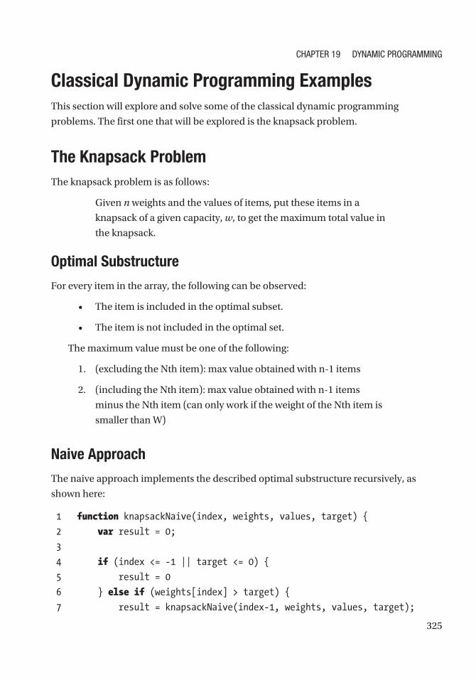
325
Classical Dynamic Programming ExamplesThis section will explore and solve some of the classical dynamic programming
problems. The first one that will be explored is the knapsack problem.
The Knapsack ProblemThe knapsack problem is as follows:
Given n weights and the values of items, put these items in a
knapsack of a given capacity, w, to get the maximum total value in
the knapsack.
Optimal Substructure
For every item in the array, the following can be observed:
• The item is included in the optimal subset.
• The item is not included in the optimal set.
The maximum value must be one of the following:
1. (excluding the Nth item): max value obtained with n-1 items
2. (including the Nth item): max value obtained with n-1 items
minus the Nth item (can only work if the weight of the Nth item is
smaller than W)
Naive Approach
The naive approach implements the described optimal substructure recursively, as
shown here:
1 function knapsackNaive(index, weights, values, target) {
2 var result = 0;
3
4 if (index <= -1 || target <= 0) {
5 result = 0
6 } else if (weights[index] > target) {
7 result = knapsackNaive(index-1, weights, values, target);
Chapter 19 DynamiC programming

326
8 } else {
9 // Case 1:
10 var current = knapsackNaive(index-1, weights, values, target)
11 // Case 2:
12 var currentPlusOther = values[index] +
13 knapsackNaive(index-1, weights, values,
target - weights[index]);
14
15 result = Math.max(current, currentPlusOther);
16 }
17 return result;
18 }
19 var weights = [1,2,4,2,5],
20 values = [5,3,5,3,2],
21 target = 10;
22 knapsackNaive(4,weights, values, target);
Time Complexity: O(2n)
Figure 19-2 shows the recursion tree for a knapsack capacity of 2 units and 3 items
of 1 unit weight. As the figure shows, the function computes the same subproblems
repeatedly and has an exponential time complexity. To optimize this, you can have the
results based on the item (reference via index) and target (weight: w).
Figure 19-2. Recursion tree for knapsack
Chapter 19 DynamiC programming
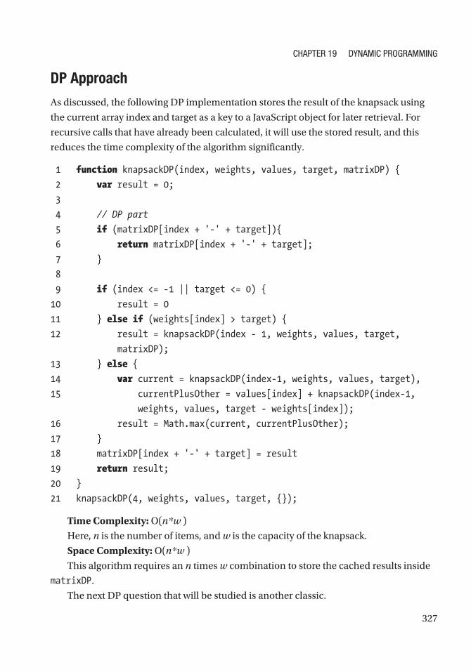
327
DP Approach
As discussed, the following DP implementation stores the result of the knapsack using
the current array index and target as a key to a JavaScript object for later retrieval. For
recursive calls that have already been calculated, it will use the stored result, and this
reduces the time complexity of the algorithm significantly.
1 function knapsackDP(index, weights, values, target, matrixDP) {
2 var result = 0;
3
4 // DP part
5 if (matrixDP[index + '-' + target]){
6 return matrixDP[index + '-' + target];
7 }
8
9 if (index <= -1 || target <= 0) {
10 result = 0
11 } else if (weights[index] > target) {
12 result = knapsackDP(index - 1, weights, values, target,
matrixDP);
13 } else {
14 var current = knapsackDP(index-1, weights, values, target),
15 currentPlusOther = values[index] + knapsackDP(index-1,
weights, values, target - weights[index]);
16 result = Math.max(current, currentPlusOther);
17 }
18 matrixDP[index + '-' + target] = result
19 return result;
20 }
21 knapsackDP(4, weights, values, target, {});
Time Complexity: O(n*w )
Here, n is the number of items, and w is the capacity of the knapsack.
Space Complexity: O(n*w )
This algorithm requires an n times w combination to store the cached results inside
matrixDP.
The next DP question that will be studied is another classic.
Chapter 19 DynamiC programming
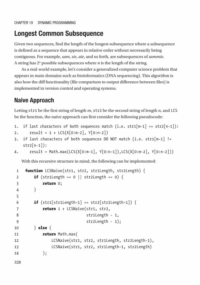
328
Longest Common SubsequenceGiven two sequences, find the length of the longest subsequence where a subsequence
is defined as a sequence that appears in relative order without necessarily being
contiguous. For example, sam, sie, aie, and so forth, are subsequences of sammie.
A string has 2n possible subsequences where n is the length of the string.
As a real-world example, let’s consider a generalized computer science problem that
appears in main domains such as bioinformatics (DNA sequencing). This algorithm is
also how the diff functionality (file comparison to output difference between files) is
implemented in version control and operating systems.
Naive Approach
Letting str1 be the first string of length m, str2 be the second string of length n, and LCS
be the function, the naive approach can first consider the following pseudocode:
1. if last characters of both sequences match (i.e. str1[m-1] == str2[n-1]):
2. result = 1 + LCS(X[0:m-2], Y[0:n-2])
3. if last characters of both sequences DO NOT match (i.e. str1[m-1] !=
str2[n-1]):
4. result = Math.max(LCS(X[0:m-1], Y[0:n-1]),LCS(X[0:m-2], Y[0:n-2]))
With this recursive structure in mind, the following can be implemented:
1 function LCSNaive(str1, str2, str1Length, str2Length) {
2 if (str1Length == 0 || str2Length == 0) {
3 return 0;
4 }
5
6 if (str1[str1Length-1] == str2[str2Length-1]) {
7 return 1 + LCSNaive(str1, str2,
8 str1Length - 1,
9 str2Length - 1);
10 } else {
11 return Math.max(
12 LCSNaive(str1, str2, str1Length, str2Length-1),
13 LCSNaive(str1, str2, str1Length-1, str2Length)
14 );
Chapter 19 DynamiC programming

329
15 }
16 }
17
18 function LCSNaiveWrapper(str1, str2) {
19 return LCSNaive(str1, str2, str1.length, str2.length);
20 }
21 LCSNaiveWrapper('AGGTAB', 'GXTXAYB'); // 4
Time Complexity: O(2n)
Figure 19-3 shows the recursion tree for SAM and BAE (visually cut off at a height
of 3). As you can see, ('SA', 'BAE') is repeated.
DP Approach
The recursive structure described can be translated into a table/cache where the rows
each represent a character in str1 and the columns each represent a character in str2.
Each item in a matrix at a row, i, and a column, j, represents LCS(str1[0:i], str2[0:j]).
1 function longestCommonSequenceLength(str1, str2) {
2 var matrix = Array(str1.length + 1).fill(Array(str2.length +
1).fill(0)),
3 rowLength = str1.length + 1,
4 colLength = str2.length + 1,
5 max = 0;
6
Figure 19-3. Recursion tree for longest common string length
Chapter 19 DynamiC programming

330
7 for (var row = 1; row < rowLength; row++) {
8 for (var col = 1; col < colLength; col++) {
9 var str1Char = str1.charAt(row - 1),
10 str2Char = str2.charAt(col - 1);
11
12 if (str1Char == str2Char) {
13 matrix[row][col] = matrix[row - 1][col - 1] + 1;
14 max = Math.max(matrix[row][col], max);
15 }
16 }
17 }
18 return max;
19 }
20 longestCommonSequenceLength('abcd', 'bc');
Time Complexity: O(m * n)
Space Complexity: O(m * n)
Here, m is the length of str1, and n is the length of str2.
Coin ChangeGiven a value/money n and an unlimited supply of each coin of different values, S = {S1,
S2, .. Sm}, of size M, how many ways can the change be made without considering the
order of the coins?
Given N=4, M=3, and S = {1,2,3}, the answer is 4.
1. 1,1,1,1,
2. 1,1,2
3. 2,2
4. 1,3
Optimal Substructure
You can observe the following about the number of coin changes:
1) Solutions without Mth coin
2) Solutions with (at least) one Mth coin
Chapter 19 DynamiC programming

331
Given that coinChange(S, M, N) is a function to count the number of coin changes,
mathematically it can be rewritten as follows by using the two observations from earlier:
coinChange(S, M, N) = coinChange(S, M-1, N) + coinChange(S, M, N-Sm)
Naive Approach
The naive approach can implement the described algorithm using recursion, as shown
here:
1 // Returns the count of ways we can sum coinArr which have
2 // index like: [0,...,numCoins]
3 function countCoinWays(coinArr, numCoins, coinValue){
4 if (coinValue == 0) {
5 // if the value reached zero, then only solution is
6 // to not include any coin
7 return 1;
8 }
9 if (coinValue < 0 || (numCoins<=0 && coinValue >= 1)) {
10 // value is less than 0 means no solution
11 // no coins left but coinValue left also means no solution
12 return 0;
13 }
14 //
15 return countCoinWays(coinArr,numCoins-1, coinValue) +
16 countCoinWays(coinArr,numCoins, coinValue- coinArr[numCoins-1]);
17 }
18 function countCoinWaysWrapper(coinArr, coinValue) {
19 return countCoinWays(coinArr, coinArr.length, coinValue);
20 }
21 countCoinWaysWrapper([1,2,3],4);
Time Complexity: O(nm)
Space Complexity: O(n)
Here, m is the number of available types of coins, and n is the desired currency to
convert into change.
Chapter 19 DynamiC programming

332
Overlapping Subproblems
You can see from the recursion tree in Figure 19-4 that there are lots of overlapping
subproblems.
To account solve for this, a table (matrix) can be used to store already computed
results.
DP Approach
The matrix for the DP approach has the coinValue number of rows and the numCoins
number of columns. Any matrix at i and j represent the number of ways given a
coinValue of i and a numCoins of j.
1 function countCoinWaysDP(coinArr, numCoins, coinValue) {
2 // creating the matrix
3 var dpMatrix = [];
4
5 for (var i=0; i <= coinValue; i++) {
6 dpMatrix[i] = [];
Figure 19-4. Recursion tree for longest coin change
Chapter 19 DynamiC programming

333
7 for(var j=0; j< numCoins; j++) {
8 dpMatrix[i][j] = undefined;
9 }
10 }
11
12 for (var i=0; i < numCoins; i++) {
13 dpMatrix[0][i] = 1;
14 }
15
16 for (var i=1; i < coinValue + 1; i++) {
17 for (var j=0; j < numCoins; j++) {
18 var temp1 = 0,
19 temp2 = 0;
20
21 if (i - coinArr[j] >= 0) {
22 // solutions including coinArr[j]
23 temp1 = dpMatrix[i - coinArr[j]][j];
24 }
25
26 if (j >= 1) {
27 // solutions excluding coinArr[j]
28 temp2 = dpMatrix[i][j-1];
29 }
30
31 dpMatrix[i][j] = temp1 + temp2;
32 }
33 }
34 return dpMatrix[coinValue][numCoins-1];
35 }
36
37 function countCoinWaysDPWrapper(coinArr, coinValue) {
38 return countCoinWaysDP(coinArr, coinArr.length, coinValue);
39 }
40 countCoinWaysDPWrapper([1,2,3],4);
Chapter 19 DynamiC programming

334
Time Complexity: O(m * n)
Space Complexity: O(m * n)
Here, m is the number of available types of coins, and n is the desired currency to
convert into change.
Edit (Levenshtein) DistanceThe edit distance problem considers the following:
Given a string (str1) of length m and another string (str2) of
length n, what is the minimum number of edits to convert str1
into str2?
The valid operations are the following:
1. Insert
2. Remove
3. Replace
Optimal Substructure
If each character is processed one by one from each str1 and str2, the following is
possible:
1. the characters are the same:
do nothing
2. the characters are different:
consider the cases recursively:
Insert: for m and n-1
Remove: for m-1 and n
Replace: for m-1 and n-1
Naive Approach
The naive approach can implement the described substructure recursively, as shown here:
1 function editDistanceRecursive(str1, str2, length1, length2) {
2 // str1 is empty. only option is insert all of str2
3 if (length1 == 0) {
Chapter 19 DynamiC programming

335
4 return length2;
5 }
6 // str2 is empty. only option is insert all of str1
7 if (length2 == 0) {
8 return length1;
9 }
10
11 // last chars are same,
12 // ignore last chars and count remaining
13 if (str1[length1-1] == str2[length2-1]) {
14 return editDistanceRecursive(str1, str2,
15 length1-1, length2-1);
16 }
17
18 // last char is not the same
19 // there are three operations: insert, remove, replace
20 return 1 + Math.min (
21 // insert
22 editDistanceRecursive(str1, str2, length1, length2-1),
23 // remove
24 editDistanceRecursive(str1, str2, length1-1, length2),
25 // replace
26 editDistanceRecursive(str1, str2, length1-1, length2-1)
27 );
28 }
29
30 function editDistanceRecursiveWrapper(str1, str2) {
31 return editDistanceRecursive(str1, str2, str1.length, str2.length);
32 }
33
34 editDistanceRecursiveWrapper('sammie','bae');
Time Complexity: O(3m)
The time complexity of the naive solution is exponential, and the worst case is when
no characters in the two strings match. This makes sense because each call has three
calls (insert, remove, replace).
Chapter 19 DynamiC programming

336
Again, you can see that the same problems are solved over and over again (see
Figure 19-5). This can be optimized by constructing a matrix that stores the already-
computed results of subproblems.
DP Approach
The dynamic programming approach will construct a matrix with the dimensions str1
and str2. The base case is when i or j is equal to 0. In other cases, it is 1 + min(insert,
remove, replace) just like the recursive approach.
1 function editDistanceDP(str1, str2, length1, length2) {
2 // creating the matrix
3 var dpMatrix = [];
4 for(var i=0; i<length1+1; i++) {
5 dpMatrix[i] = [];
6 for(var j=0; j<length2+1; j++) {
7 dpMatrix[i][j] = undefined;
8 }
9 }
10
11 for (var i=0; i < length1 + 1; i++) {
12 for (var j=0; j < length2 + 1; j++) {
13 // if first str1 is empty,
Figure 19-5. Recursion tree for edit distance
Chapter 19 DynamiC programming

337
14 // have to insert all the chars of str2
15 if (i == 0) {
16 dpMatrix[i][j] = j;
17 } else if (j == 0) {
18 dpMatrix[i][j] = i;
19 } else if (str1[i-1] == str2[j-1]) {
20 // if the same, no additional cost
21 dpMatrix[i][j] = dpMatrix[i-1][j-1];
22 } else {
23 var insertCost = dpMatrix[i][j-1],
24 removeCost = dpMatrix[i-1][j],
25 replaceCost= dpMatrix[i-1][j-1];
26
27 dpMatrix[i][j] = 1 + Math.min(insertCost,removeCost,
replaceCost);
28 }
29 }
30 }
31 return dpMatrix[length1][length2];
32 }
33
34 function editDistanceDPWrapper(str1, str2) {
35 return editDistanceDP(str1, str2, str1.length, str2.length);
36 }
37
38 editDistanceDPWrapper('sammie','bae');
Time Complexity: O(m * n)
Space Complexity: O(m * n)
Here, m is the length of str1, and n is the length of str2.
Chapter 19 DynamiC programming

338
SummaryDynamic programming can be utilized to optimize an algorithm if the following
conditions are satisfied:
• Optimal substructure: The optimal solution to the problem contains
optimal solutions to its subproblems.
• Overlapping subproblems: The solutions for subproblems are needed
multiple times.
To store the already computed solutions to a subproblem, a matrix or a hash
table is typically used; this is because both provide O(1) lookup time. Doing this,
the time complexity can be improved from exponential (e.g., O(2n )) to polynomial
time (e.g., O(n 2)).
Chapter 19 DynamiC programming

339© Sammie Bae 2019 S. Bae, JavaScript Data Structures and Algorithms, https://doi.org/10.1007/978-1-4842-3988-9_20
CHAPTER 20
Bit ManipulationBit manipulation is an advanced topic that JavaScript developers typically do not need
to know. Low-level programming languages such as C take advantage of these operators.
However, you should learn a bit about bit manipulation if you want to implement high-
performance server-side code.
Understanding bit manipulation requires some knowledge of digital logic. Any
introductory course in discrete math or circuits would be helpful to understand these
concepts.
Bitwise OperatorsHere are the bitwise operators in JavaScript:
• & : AND
• | : OR
• ~ : NOT
• ^ : XOR
• <<: Left shift
• >>: Right shift
• >>>: Zero-fill right shift
Note Recall from Chapter 3 that all numbers are represented with 32 bits (meaning there are 32 1s and 0s). When converting from decimal numbers (base 10) to binary (base 2), it is important to keep this in mind.
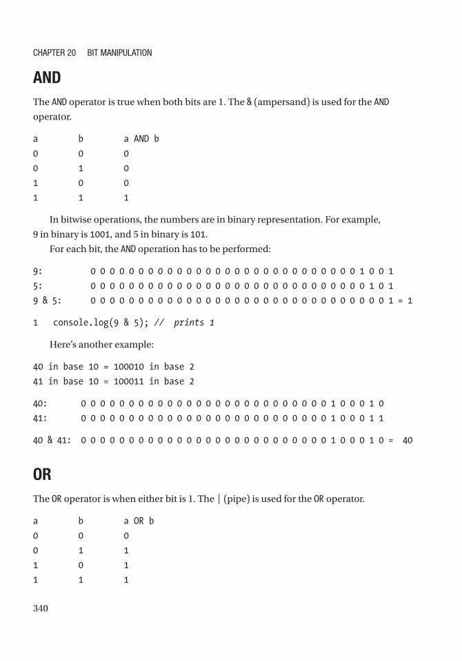
340
ANDThe AND operator is true when both bits are 1. The & (ampersand) is used for the AND
operator.
a b a AND b
0 0 0
0 1 0
1 0 0
1 1 1
In bitwise operations, the numbers are in binary representation. For example,
9 in binary is 1001, and 5 in binary is 101.
For each bit, the AND operation has to be performed:
9: 0 0 0 0 0 0 0 0 0 0 0 0 0 0 0 0 0 0 0 0 0 0 0 0 0 0 0 0 1 0 0 1
5: 0 0 0 0 0 0 0 0 0 0 0 0 0 0 0 0 0 0 0 0 0 0 0 0 0 0 0 0 0 1 0 1
9 & 5: 0 0 0 0 0 0 0 0 0 0 0 0 0 0 0 0 0 0 0 0 0 0 0 0 0 0 0 0 0 0 0 1 = 1
1 console.log(9 & 5); // prints 1
Here’s another example:
40 in base 10 = 100010 in base 2
41 in base 10 = 100011 in base 2
40: 0 0 0 0 0 0 0 0 0 0 0 0 0 0 0 0 0 0 0 0 0 0 0 0 0 0 1 0 0 0 1 0
41: 0 0 0 0 0 0 0 0 0 0 0 0 0 0 0 0 0 0 0 0 0 0 0 0 0 0 1 0 0 0 1 1
40 & 41: 0 0 0 0 0 0 0 0 0 0 0 0 0 0 0 0 0 0 0 0 0 0 0 0 0 0 1 0 0 0 1 0 = 40
ORThe OR operator is when either bit is 1. The | (pipe) is used for the OR operator.
a b a OR b
0 0 0
0 1 1
1 0 1
1 1 1
ChapteR 20 Bit Manipulation
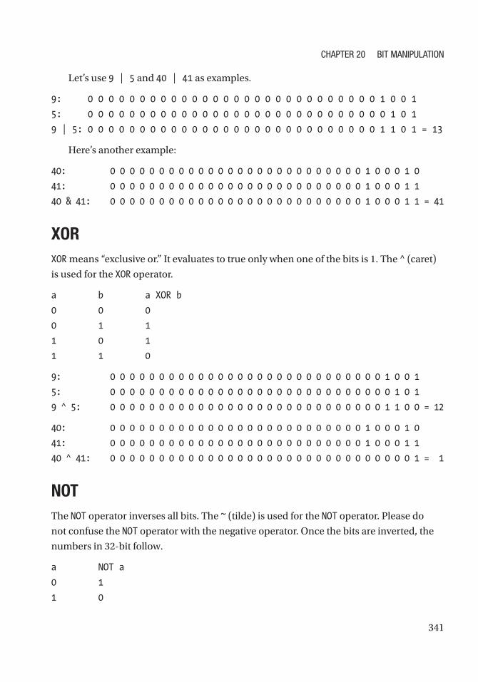
341
Let’s use 9 | 5 and 40 | 41 as examples.
9: 0 0 0 0 0 0 0 0 0 0 0 0 0 0 0 0 0 0 0 0 0 0 0 0 0 0 0 0 1 0 0 1
5: 0 0 0 0 0 0 0 0 0 0 0 0 0 0 0 0 0 0 0 0 0 0 0 0 0 0 0 0 0 1 0 1
9 | 5: 0 0 0 0 0 0 0 0 0 0 0 0 0 0 0 0 0 0 0 0 0 0 0 0 0 0 0 0 1 1 0 1 = 13
Here’s another example:
40: 0 0 0 0 0 0 0 0 0 0 0 0 0 0 0 0 0 0 0 0 0 0 0 0 0 0 1 0 0 0 1 0
41: 0 0 0 0 0 0 0 0 0 0 0 0 0 0 0 0 0 0 0 0 0 0 0 0 0 0 1 0 0 0 1 1
40 & 41: 0 0 0 0 0 0 0 0 0 0 0 0 0 0 0 0 0 0 0 0 0 0 0 0 0 0 1 0 0 0 1 1 = 41
XORXOR means “exclusive or.” It evaluates to true only when one of the bits is 1. The ^ (caret)
is used for the XOR operator.
a b a XOR b
0 0 0
0 1 1
1 0 1
1 1 0
9: 0 0 0 0 0 0 0 0 0 0 0 0 0 0 0 0 0 0 0 0 0 0 0 0 0 0 0 0 1 0 0 1
5: 0 0 0 0 0 0 0 0 0 0 0 0 0 0 0 0 0 0 0 0 0 0 0 0 0 0 0 0 0 1 0 1
9 ^ 5: 0 0 0 0 0 0 0 0 0 0 0 0 0 0 0 0 0 0 0 0 0 0 0 0 0 0 0 0 1 1 0 0 = 12
40: 0 0 0 0 0 0 0 0 0 0 0 0 0 0 0 0 0 0 0 0 0 0 0 0 0 0 1 0 0 0 1 0
41: 0 0 0 0 0 0 0 0 0 0 0 0 0 0 0 0 0 0 0 0 0 0 0 0 0 0 1 0 0 0 1 1
40 ^ 41: 0 0 0 0 0 0 0 0 0 0 0 0 0 0 0 0 0 0 0 0 0 0 0 0 0 0 0 0 0 0 0 1 = 1
NOTThe NOT operator inverses all bits. The ~ (tilde) is used for the NOT operator. Please do
not confuse the NOT operator with the negative operator. Once the bits are inverted, the
numbers in 32-bit follow.
a NOT a
0 1
1 0
ChapteR 20 Bit Manipulation

342
Let’s take 9 and 5 as an example:
9: 0 0 0 0 0 0 0 0 0 0 0 0 0 0 0 0 0 0 0 0 0 0 0 0 0 0 0 0 1 0 0 1
~9: 1 1 1 1 1 1 1 1 1 1 1 1 1 1 1 1 1 1 1 1 1 1 1 1 1 1 1 1 0 1 1 0 = -10
5: 0 0 0 0 0 0 0 0 0 0 0 0 0 0 0 0 0 0 0 0 0 0 0 0 0 0 0 0 0 1 0 1
~5: 1 1 1 1 1 1 1 1 1 1 1 1 1 1 1 1 1 1 1 1 1 1 1 1 1 1 1 1 1 0 1 0 = -6
Left ShiftIn left shift, all the bits are shifted to the left, and any excess bits shifted off to the left are
discarded. The << (double left-angle brackets) is the operator of left shift.
9: 0 0 0 0 0 0 0 0 0 0 0 0 0 0 0 0 0 0 0 0 0 0 0 0 0 0 0 0 1 0 0 1
9 << 1: 0 0 0 0 0 0 0 0 0 0 0 0 0 0 0 0 0 0 0 0 0 0 0 0 0 0 0 1 0 0 1 0 = 18
9 << 2: 0 0 0 0 0 0 0 0 0 0 0 0 0 0 0 0 0 0 0 0 0 0 0 0 0 0 1 0 0 1 0 0 = 36
Left shift often multiplies elements by 2 for each shift. This is because binary is a
base 2 system, implying a left shift is equal to multiplying all the digits by 2. However,
the shift can cause the bit to overflow and reduce the value.
1073741833: 0 1 0 0 0 0 0 0 0 0 0 0 0 0 0 0 0 0 0 0 0 0 0 0 0 0 0 0 1
0 0 1
1073741833 << 2: 0 0 0 0 0 0 0 0 0 0 0 0 0 0 0 0 0 0 0 0 0 0 0 0 0 0 1 0 0
1 0 0 = 36
Right ShiftIn right shift, all the bits are shifted to the right, and any excess bits shifted off to the right
are discarded. The >> (double right angle brackets) is the operator for right shift.
9: 0 0 0 0 0 0 0 0 0 0 0 0 0 0 0 0 0 0 0 0 0 0 0 0 0 0 0 0 1 0 0 1
9 >> 1: 0 0 0 0 0 0 0 0 0 0 0 0 0 0 0 0 0 0 0 0 0 0 0 0 0 0 0 0 0 1 0 0 = 4
-9: 1 1 1 1 1 1 1 1 1 1 1 1 1 1 1 1 1 1 1 1 1 1 1 1 1 1 1 1 0 1 1 1
-9 >> 2: 1 1 1 1 1 1 1 1 1 1 1 1 1 1 1 1 1 1 1 1 1 1 1 1 1 1 1 1 1 1 0 1 = -3
ChapteR 20 Bit Manipulation

343
In this example, shifting divided the 9 by 2 (integer division). This is because, again,
binary is a base 2 system.
Zero-Fill Right ShiftIn zero-fill right shift, all the bits are shifted to the right, and any excess bits shifted off
to the right are discarded. However, the sign bit (the leftmost bit) becomes a 0 before
the shift, and this results in a non-negative number. The >>> (triple right brackets) is the
operator for the zero-fill right shift.
-9: 1 1 1 1 1 1 1 1 1 1 1 1 1 1 1 1 1 1 1 1 1 1 1 1 1 1 1 1 0 1 1 1
-9 >>> 1: 0 1 1 1 1 1 1 1 1 1 1 1 1 1 1 1 1 1 1 1 1 1 1 1 1 1 1 1 1 0 1 1 =
2147483643
In this example, shifting divided the 9 by 2 (integer division). This is because, again,
binary is a base 2 system.
To have a better understanding of why these operations work, it is recommended to
take an introductory digital logic course in school or online. In the end, everything consists
of 1s and 0s because a transistor in a computer can have only two states: on and off.
Number OperationsThis section will cover how to perform addition, subtraction, multiplication, division,
and modulus using bitwise operators.
AdditionAdding binary numbers is no different from adding decimal numbers. The rule that
children learn in the second grade is the same: add up two numbers and carry 1 to next
digit if it exceeds 10.
The function that implements this is as follows. You can find all the code on GitHub.1
1 function BitwiseAdd(a, b){
2 while (b != 0) {
3 var carry = (a & b);
1 https://github.com/Apress/js-data-structures-and-algorithms
ChapteR 20 Bit Manipulation

344
4 a = a ^ b;
5 b = carry << 1;
6 }
7 return a;
8 }
9
10 console.log(BitwiseAdd(4,5)); // 9
Here are two examples in detail:
bitwiseAdd(4, 5);
4: 0 0 0 0 0 0 0 0 0 0 0 0 0 0 0 0 0 0 0 0 0 0 0 0 0 0 0 0 0 1 0 0
5: 0 0 0 0 0 0 0 0 0 0 0 0 0 0 0 0 0 0 0 0 0 0 0 0 0 0 0 0 0 1 0 1
sum = 4 ^ 5 = 0 0 0 0 0 0 0 0 0 0 0 0 0 0 0 0 0 0 0 0 0 0 0 0 0 0 0 0 0 0 0 1
= 1 (base 10)
carry = (a & b) << 1
a & b = 0 0 0 0 0 0 0 0 0 0 0 0 0 0 0 0 0 0 0 0 0 0 0 0 0 0 0 0 0 1 0 0
(a & b) << 1 = 0 0 0 0 0 0 0 0 0 0 0 0 0 0 0 0 0 0 0 0 0 0 0 0 0 0 0 0 1 0 0 0
= 8 (base 10)
bitwiseAdd(1, 8);
1: 0 0 0 0 0 0 0 0 0 0 0 0 0 0 0 0 0 0 0 0 0 0 0 0 0 0 0 0 0 0 0 1
8: 0 0 0 0 0 0 0 0 0 0 0 0 0 0 0 0 0 0 0 0 0 0 0 0 0 0 0 0 1 0 0 0
sum = 1 ^ 8 = 0 0 0 0 0 0 0 0 0 0 0 0 0 0 0 0 0 0 0 0 0 0 0 0 0 0 0 0 1 0 0 1
= 9 (base 10)
carry = (a & b) << 1
a & b = 0 0 0 0 0 0 0 0 0 0 0 0 0 0 0 0 0 0 0 0 0 0 0 0 0 0 0 0 0 0 0 0
-> return 9 (a)
SubtractionSubtraction is the difference of two numbers. However, you can also think of it as adding
a negative number. Here’s an example: 5 - 4 = 5 + (-4).
Therefore, first create a negate function using the NOT operator. In binary, subtracting
a negative binary number from a positive one is obtained by inverting all the bits and
adding 1. This is implemented in the following code block:
ChapteR 20 Bit Manipulation
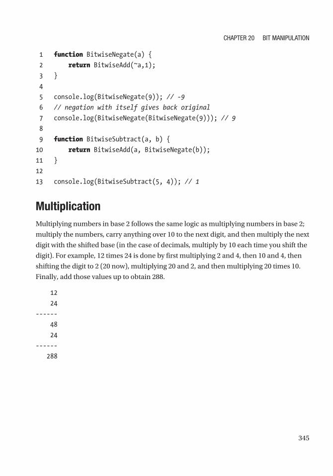
345
1 function BitwiseNegate(a) {
2 return BitwiseAdd(~a,1);
3 }
4
5 console.log(BitwiseNegate(9)); // -9
6 // negation with itself gives back original
7 console.log(BitwiseNegate(BitwiseNegate(9))); // 9
8
9 function BitwiseSubtract(a, b) {
10 return BitwiseAdd(a, BitwiseNegate(b));
11 }
12
13 console.log(BitwiseSubtract(5, 4)); // 1
MultiplicationMultiplying numbers in base 2 follows the same logic as multiplying numbers in base 2;
multiply the numbers, carry anything over 10 to the next digit, and then multiply the next
digit with the shifted base (in the case of decimals, multiply by 10 each time you shift the
digit). For example, 12 times 24 is done by first multiplying 2 and 4, then 10 and 4, then
shifting the digit to 2 (20 now), multiplying 20 and 2, and then multiplying 20 times 10.
Finally, add those values up to obtain 288.
12
24
------
48
24
------
288
ChapteR 20 Bit Manipulation

346
In binary:
0 1 1 0 0
1 1 0 0 0
-----------------
0 0 0 0 0
0 0 0 0 0
0 0 0 0 0
0 1 1 0 0
0 1 1 0 0
-------------
1 0 0 1 0 0 0 0 0
The following code block illustrates this implementation, and it also handles
negative numbers:
1 function BitwiseMultiply(a, b) {
2 var m = 1,
3 c = 0;
4
5 if (a < 0) {
6 a = BitwiseNegate(a);
7 b = BitwiseNegate(b);
8 }
9 while (a >= m && b) {
10 if (a & m) {
11 c = BitwiseAdd(b, c);
12 }
13 b = b << 1;
14 m = m << 1;
15 }
16 return c;
17 }
18 console.log(BitwiseMultiply(4, 5)); // 20
ChapteR 20 Bit Manipulation

347
DivisionDivision can be thought of as the number of times you can subtract b from a, given a/b.
For example, 4/2 = 2 because 4-2-2 = 0. Using this property, bitwise division can be
implemented as follows:
1 function BitwiseDividePositive(a, b) {
2 var c = 0;
3
4 if (b != 0) {
5 while (a >= b) {
6 a = BitwiseSubtract(a, b);
7 c++;
8 }
9 }
10 return c;
11 }
12 console.log(BitwiseDividePositive(10, 2)); // 5
This is relatively simple for positive numbers. The while loop can keep subtracting,
and a counter variable can store how many times b subtracted a. However, what about
for negative numbers? -10 /2 = -5, but we cannot subtract 2 from -10 because the while
loop would go on forever. To avoid this, convert both the numbers into positive numbers.
Doing this, we have to keep track of the sign.
a b a * b
+ + +
+ - -
- + -
- - +
If negative is represented as 1 and positive as 0, this is the same table as an XOR table:
a b a * b
0 0 0
0 1 1
1 0 1
1 1 0
ChapteR 20 Bit Manipulation

348
The division algorithm is shown next. This function subtracts b from a until it is zero.
Again, negative numbers have to be handled appropriately at the end with a negation
helper function.
1 function BitwiseDivide(a, b) {
2 var c = 0,
3 isNegative = 0;
4
5 if (a < 0) {
6 a = BitwiseNegate(a); // convert to positive
7 isNegative = !isNegative;
8 }
9
10 if (b < 0) {
11 b = BitwiseNegate(b); // convert to positive
12 isNegative = !isNegative;
13 }
14
15 if (b != 0) {
16 while (a >= b) {
17 a = BitwiseSubtract(a, b);
18 c++;
19 }
20 }
21
22 if (isNegative) {
23 c = BitwiseNegate(c);
24 }
25
26 return c;
27 }
28
29 console.log(BitwiseDivide(10, 2)); // 5
30 console.log(BitwiseDivide(-10, 2)); // -5
31 console.log(BitwiseDivide(-200, 4)); // -50
ChapteR 20 Bit Manipulation

349
SummaryThis chapter covered the basics of bit manipulation in JavaScript. Bit manipulation
is used for high-performance numerical operations. Using bitwise operators is much
faster than using the native methods in the Math class. With JavaScript advancing into
server-side programming with Node.js, more efficient code is needed. To consolidate the
concepts from this chapter, Table 20-1 summarizes bitwise operators and their usage.
Table 20-1. Bit Manipulation Summary
Operator Operation Use Case
& AND 1 when both bits are 1
| OR 1 when either bit is 1
∼ NOT inverts all the bits
^ XOR 1 when only one of the bits is 1
<< left shift Shifts to the left, and any excess bits are shifted off
>> Right shift Shifts to the right, and any excess bits are shifted off
>>> Zero-fill right shift Shifts to the right, and any excess bits are shifted off and the
sign bit comes 0
ChapteR 20 Bit Manipulation

351© Sammie Bae 2019 S. Bae, JavaScript Data Structures and Algorithms, https://doi.org/10.1007/978-1-4842-3988-9
Index
AAccess queue, 170–171Access stacks, 166–167Algorithm
Boyer–Moore string search, 307KMP string search, 311Rabin–Karp search, 316
AND operator, 340Arrays
access, 54deletion, 54exercises
matrix rotation, 79–81path finding, 75–79spiral print, 71–73tic-tac-toe check, 73–74
functional array methods, 67helper functions, 57insertion, 53–54iteration, 54K-sorted arrays, 66–67largest value, 270median of two sorted
arrays, 63–65multidimensional arrays, 68.slice() function, 62–63smallest value, 270
Ascending-Order sort, 261–264.atob() function, 42
AVL treesdeletion, 230–231double rotation
rotate left right, 227rotate right left, 225–226
insertion, 229–230result, 231–232single rotation
rotate left, 222–223rotate right, 223, 225
tree balancing, 228
BBase64 encoding, 42–43Big-O notation
coefficient rule, 5–6complexities, 2–3fundamental rules, 4master theorem, 106–107O(n) algorithm, 2polynomial rule, 8product rule, 7–8recurrence relations, 105–106sum rule, 6
Binary heapmax-heap, 254–257percolation
bubble up/down, 250implementation, 253–254

352
max-heap structure, 255–257min-heap structure, 251–252
Binary search algorithm, 127–128, 143Binary search trees (BSTs), 214
deletion, 218–219insertion, 216, 218nth distance, root, 237–238result, 233search, 220
Binary tree, 206, 234–237, 239–241Bioinformatics, 328Bit manipulation, 339Bitwise operators
AND, 340left shift, 342NOT, 341OR, 340–341right shift, 342XOR, 341zero-fill right shift, 343
Bottom variable declaration, 14Boyer–Moore string
search, 307–311Breadth-first search (BFS), 212
end node, 288–289graph, 286–287level-order traversal, 286search algorithm, 286start node, 288undirected graph, 287
btoa() function, 42Bubble sorting, 129, 131
CCaching
LFU (see Least frequently used (LFU) caching)
LRU (see Least recently used (LRU) caching)
spatial locality, 193temporal locality, 193
Coefficient rule, 5–6Coin change, 330–334Constructor, 85–86Count sort, 140Cyclical graph, 276–277
DDeletion, queue, 169–170Deletion stacks, 166Dense graph, 276Depth-first search (DFS)
graph, 290post-order tree traversal, 289time complexity, 291
dequeuing, 168Descending-Order sort, 264–266Dijkstra’s algorithm
_extractMin method, 295, 297fibonacci heap, 297shortest path, 294stage 1, 294stage 2, 295
Directed graphsadding vertex, 284edges property, 283origin vertex, 283removing vertex, 285
Divide-and-conquer method, 101
Doubly linked listdeletion, head, 186–187deletion, tail, 187–188insertion, head, 185insertion, tail, 185–186
Binary heap (cont.)
Index

353
nodes, 184search, 188–189
Dynamic programming (DP), 323coin change, 330–332, 334edit (Levenshtein)
distance, 334–337Knapsack problem, 325–327longest common
subsequence, 328–330motivations, 321–322rules, 323–324
EEdit (Levenshtein)
distance, 334–337Encoding, 41–42Encryption, 45–46enqueuing, 168
FFibonacci sequence, 101, 321–322First in, first
out (FIFO), 167Functional array methods
filter, 68map, 67reduce, 68
GGraphs
applications, 273cyclical, 276–277definition, 273degree of vertex, 275dense, 276edge, 274
sparse, 275vertex, 274weighted edges, 293
Graph traversalBFS, 286DFS, 289techniques, 285
HHashtables
get() function, 152implementation
double-hashing, 160–161linear probing, 156–158quadratic probing, 158–159
localStorage, 152put() function, 152technique
prime numbers, 152–154probing, 154rehashing/double-hashing, 155
Heapsbinary heap (see Binary heap)indices, 246max-heap, 246–247
complete implementation, 259, 261sorting, 264–266
min-heap, 247complete
implementation, 258–259sorting, 261–264
node index summary, 267operations summary, 267relationship, 248sorting
ascending-order, 261–264descending-order, 264–266
Heap sort, 261
Index

354
Helper functions.concat(), 59.length property, 59.slice(begin,end), 57–58.splice(begin,size,element1,
element2…), 58–59spread operator, 60
IIn-order traversal, 209–210Insertion
queue, 169sort, 132, 134stacks, 165
insideIf variable, 15isSuperSet function, 119Iteration
forEach(), 56for ( in ), 56for ( of ), 56for (variables, condition,
modification), 55
JJagged array, 69JavaScript
block scope, 15–16functional scope, 13, 15global scope, 13infinity, 26integer division, 23–24maximums, 24minimums, 25Number.EPSILON, 24object property, 83objects, 18–20
primality test, 26–27true/false checking, 17=== vs == type, 18
KKnapsack problem, 325–327Knuth–Morris–Pratt string
search, 311–316
LLast in, first out (LIFO), 163Least frequently used (LFU)
caching, 193–194doubly linked list, 194–195get implementation, 198hash tables, 195hybrid systems, 194set implementation, 196usage, 199
Least recently used (LRU) caching, 193, 199
doubly linked list, 199–201get implementation, 201set implementation, 202
.length property, 59Level-order traversal, 212–213Linear probing, 154Linear search, 125–126Linked list, 179Longest common
subsequence, 328–330
MMatrix rotation, 79–81Max-Heap, 254–257
Index

355
Memoization, 323Memory leaks, 89–90
delete operator, 92DOM elements, 90–91global window object, 91–92
Mergesort, 138–140Min-Heap
root node, 250structure, 251–252
Mirror trees, 241–243Multidimensional arrays, 68–70
NNOT operator, 341Number operations
addition, 343–344division, 347–348multiplication, 345–346subtraction, 344–345
Number system, 21–23
OOptimal substructure, 323OR operator, 340–341
PPascal’s triangle, 103–104Path finding, 75–79Peek queue, 169Peek stacks, 165Polynomial rule, 8.pop() method, 54Post-order traversal, 211–212Pre-order traversal, 207–208Primality test, 26–27
Prime factorization, 28Prime number hashing, 152–154Probing hashing
technique, 154–155Product rule, 7–8Prototypal inheritance, 84–85Public-key encryption, 29, 46.push(element) method, 53
QQuadratic probing, 155Queue
access, 170–171deletion, 169–170FIFO, 168insertion, 169peek, 169search, 171
Quickselect, 137–138Quicksort, 134–137
RRabin–Karp search, 316
application, 319fingerprint, 316–319
Random number generation, 29Recursion
base case, 100divide-and-conquer
method, 101exercises
decimal to binary conversion, 109–110
flatten an object, 112–114palindrome, 114–115permutations, array, 110–112
Index

356
fibonacci sequenceiterative solution, 101recursive solution, 102tail recursion, 102–103
Pascal’s triangle, 103–104Recursive call stack memory, 107–109Recursive functions, 99Regular expressions
regexesany numeric characters, 40floating numeric characters, 40only alphanumeric characters, 40only numeric characters, 40query string, 41
.replace(string, replaceString), 38Root node, 205RSA encryption, 46–50
SSearching
binary, 127–128linear, 125–126stacks, 167
Search queue, 171Secure sockets layer (SSL), 45Selection sorting, 131–132Set
definition, 117operation, 118utility functions, 119–120
.shift() method, 54Singly linked list
deletion, head, 182–183deletion, value, 181–182head, 180insertion, 180–181node removal, 181
reverse, 190search, 183
.slice() function, 62Sortable stack, 177Sorting
bubble, 129–131count, 140insertion, 132–134mergesort, 138–140quickselect, 137–138quicksort, 134–137selection, 131–132built-in sort() method, 141–142
Sparse graph, 275Spatial locality, 193Spiral print, 71–73Stack overflow, 100Stacks
access, 166–167deletion, 166insertion, 165LIFO, 164peek, 165search, 167
String primitiveaccess, 35comparison, 36decomposition, 38replace, 38search, 36–37
String shortening, 43–45Sum rule, 6
TTail recursive function, 102–103Temporal locality, 193Tic-tac-toe check, 73–74Topological sort, 298–300
Recursion (cont.)
Index

357
Tree traversalin-order, 209–210level-order, 212–213post-order, 211–212pre-order, 207–208
Trie (prefix Tree), 303–307
UUnbalanced binary
search tree, 215–216Undirected graphs
adjacency list, 278adjacency matrix, 278
edges and verticesadding, 279–280removing, 280–282
nondirectional edges, 277
V, WVariable, 85
types, 16Variable hoisting, 13
X, Y, ZXOR operator, 341
Index