jacket
DESCRIPTION
jacket designTRANSCRIPT

Structural Modeling - 1
Part 1 - Structural modeling
In windows file explorer, Create “Training Project” directory, and create “Structural Modeling” subdirectory. In SACS executive, use “Settings” > “SACS System Configuration”, make sure default units set to “Metric KN Force”. Set current working directory to “Structural Modeling” and launch Precede program and using following data, Creating Jacket, Select “Create New Model” and input “TEST MODEL WITH WEIGHT CAPABILITIES” for title. Select “Jacket” in Structure Wizard and check “Generate Seastate hydrodynamic overrides”. 4 Leg 4 Pile (ungrouted) jacket platform Water depth 79.5 m Working point elevation: 4.0 m Pile connecting elev: 3.0 m Mudline elevation and pile stub elevation: -79.5m Other intermediate elevations: -50.0, -21.0, 2.0, 15.3, 23.0 m Conductors: None Skirt Piles: None Working point spacing: X1=15 m, Y1=10 m Pile/Leg Batter: Row 1 (leg 1 and leg 5, left two legs) X=0, Y=10 Row 2 (leg 3 and leg 7, right two legs) X=10, Y=10 Save model to SACINP.DAT file. Define member properties; Member Group LG1, LG2, LG3, Segment 1: D = 107 cm, T = 3.5 cm, Fy = 34.50 kN/cm2, Segment Length = 1.0 m Segment 2: D = 105 cm, T = 2.5 cm, Fy = 24.80 kN/cm2 Segment 3: D = 107 cm, T = 3.5 cm, Fy = 34.50 kN/cm2, Segment Length = 1.0 m
Structural Modeling - 2
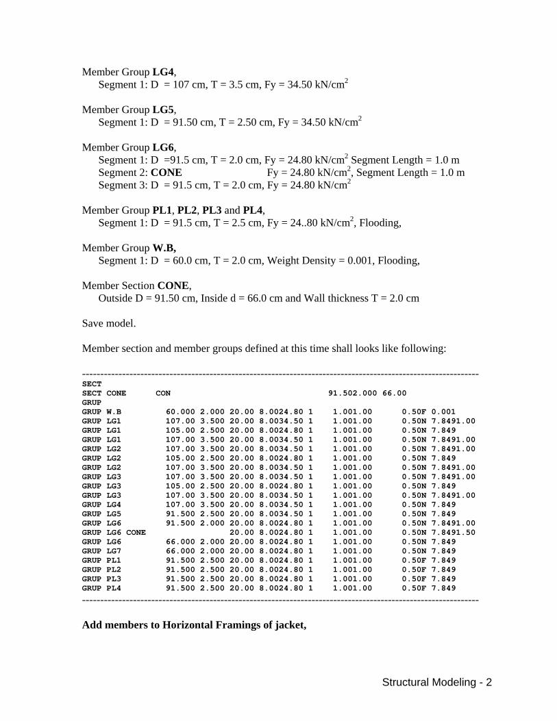
Member Group LG4, Segment 1: D = 107 cm, T = 3.5 cm, Fy = 34.50 kN/cm2 Member Group LG5, Segment 1: D = 91.50 cm, T = 2.50 cm, Fy = 34.50 kN/cm2 Member Group LG6, Segment 1: D =91.5 cm, T = 2.0 cm, Fy = 24.80 kN/cm2 Segment Length = 1.0 m Segment 2: CONE Fy = 24.80 kN/cm2, Segment Length = 1.0 m Segment 3: D = 91.5 cm, T = 2.0 cm, Fy = 24.80 kN/cm2 Member Group PL1, PL2, PL3 and PL4, Segment 1: D = 91.5 cm, T = 2.5 cm, Fy = 24..80 kN/cm2, Flooding, Member Group W.B, Segment 1: D = 60.0 cm, T = 2.0 cm, Weight Density = 0.001, Flooding, Member Section CONE, Outside D = 91.50 cm, Inside d = 66.0 cm and Wall thickness T = 2.0 cm Save model. Member section and member groups defined at this time shall looks like following: ------------------------------------------------------------------------------------------------------------- SECT SECT CONE CON 91.502.000 66.00 GRUP GRUP W.B 60.000 2.000 20.00 8.0024.80 1 1.001.00 0.50F 0.001 GRUP LG1 107.00 3.500 20.00 8.0034.50 1 1.001.00 0.50N 7.8491.00 GRUP LG1 105.00 2.500 20.00 8.0024.80 1 1.001.00 0.50N 7.849 GRUP LG1 107.00 3.500 20.00 8.0034.50 1 1.001.00 0.50N 7.8491.00 GRUP LG2 107.00 3.500 20.00 8.0034.50 1 1.001.00 0.50N 7.8491.00 GRUP LG2 105.00 2.500 20.00 8.0024.80 1 1.001.00 0.50N 7.849 GRUP LG2 107.00 3.500 20.00 8.0034.50 1 1.001.00 0.50N 7.8491.00 GRUP LG3 107.00 3.500 20.00 8.0034.50 1 1.001.00 0.50N 7.8491.00 GRUP LG3 105.00 2.500 20.00 8.0024.80 1 1.001.00 0.50N 7.849 GRUP LG3 107.00 3.500 20.00 8.0034.50 1 1.001.00 0.50N 7.8491.00 GRUP LG4 107.00 3.500 20.00 8.0034.50 1 1.001.00 0.50N 7.849 GRUP LG5 91.500 2.500 20.00 8.0034.50 1 1.001.00 0.50N 7.849 GRUP LG6 91.500 2.000 20.00 8.0024.80 1 1.001.00 0.50N 7.8491.00 GRUP LG6 CONE 20.00 8.0024.80 1 1.001.00 0.50N 7.8491.50 GRUP LG6 66.000 2.000 20.00 8.0024.80 1 1.001.00 0.50N 7.849 GRUP LG7 66.000 2.000 20.00 8.0024.80 1 1.001.00 0.50N 7.849 GRUP PL1 91.500 2.500 20.00 8.0024.80 1 1.001.00 0.50F 7.849 GRUP PL2 91.500 2.500 20.00 8.0024.80 1 1.001.00 0.50F 7.849 GRUP PL3 91.500 2.500 20.00 8.0024.80 1 1.001.00 0.50F 7.849 GRUP PL4 91.500 2.500 20.00 8.0024.80 1 1.001.00 0.50F 7.849
------------------------------------------------------------------------------------------------------------- Add members to Horizontal Framings of jacket,

Structural Modeling - 3
Plane XY for Z=-79.50 Add 4 horizontals H11 and breaking them in equal part, make joint name start from 1000. Add 4 diamond shape diagonals H12. Plane XY for Z=-50.00 Add 4 horizontals H21 and breaking them in equal part, make joint name start from 2000. Add 4 diamond shape diagonals H22. Plane XY for Z=-21.00 Add 4 horizontals H31. Add X-brace support, input Center Joint = 3000 and group label H32 and follow joint orders. Plane XY for Z=2.00 Add 4 horizontals H41. Add X-brace support, input Center Joint =4000 and group label H42 and follow joint orders. Save model. Define horizontal member properties; Member Group H11, Segment 1: D = 66.0 cm, T = 2.5 cm Member Group H12, Segment 1: D = 62.0 cm, T = 2.0 cm Member Group H21, Segment 1: D = 50.75 cm, T = 2.0 cm Member Group H22, H31 and H32, Segment 1: D = 40.75 cm, T = 1.5 cm Member Group H41 and H42, Segment 1: D = 30.375 cm, T = 1.25 cm Horizontal member groups defined at this time shall looks like following: ------------------------------------------------------------------------------------------------------------- GRUP H11 66.000 2.500 20.00 8.0024.80 1 1.001.00 0.50N 7.849 GRUP H12 62.000 2.000 20.00 8.0024.80 1 1.001.00 0.50N 7.849 GRUP H21 50.750 2.000 20.00 8.0024.80 1 1.001.00 0.50N 7.849 GRUP H22 40.750 1.500 20.00 8.0024.80 1 1.001.00 0.50N 7.849 GRUP H31 40.750 1.500 20.00 8.0024.80 1 1.001.00 0.50N 7.849 GRUP H32 40.750 1.500 20.00 8.0024.80 1 1.001.00 0.50N 7.849 GRUP H41 32.375 1.250 20.00 8.0024.80 1 1.001.00 0.50N 7.849 GRUP H42 32.375 1.250 20.00 8.0024.80 1 1.001.00 0.50N 7.849
------------------------------------------------------------------------------------------------------------- Add diagonal members to jacket rows,
Structural Modeling - 4
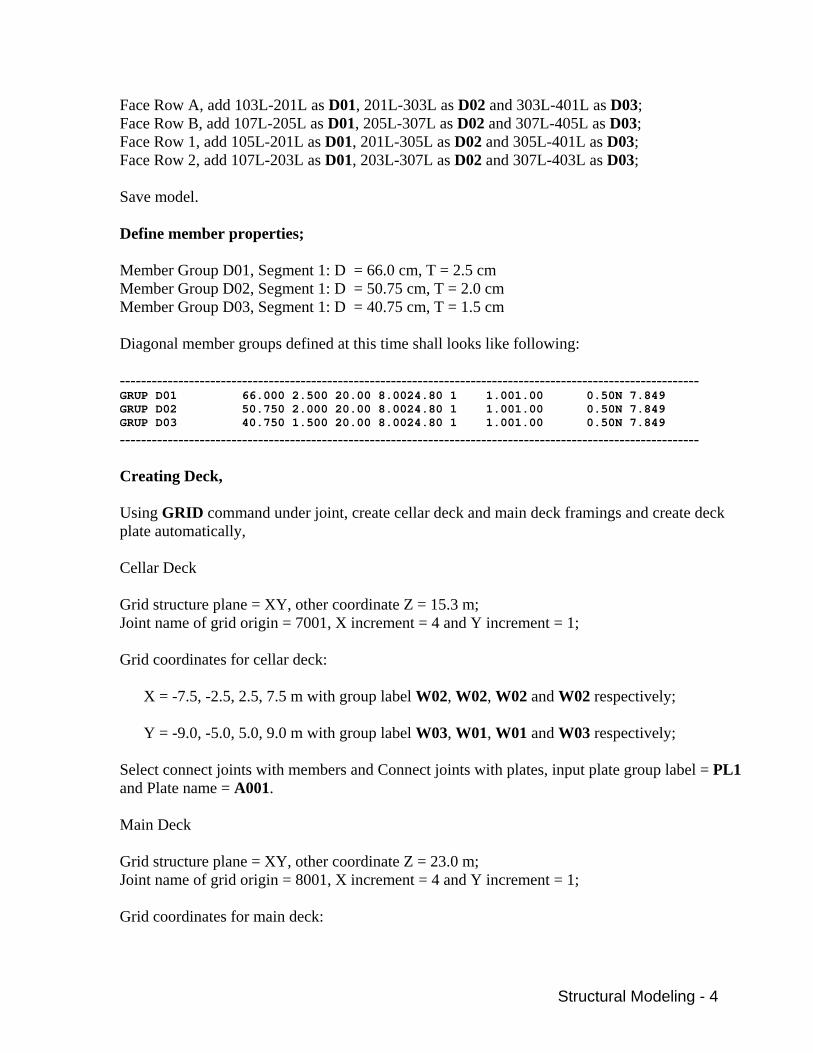
Face Row A, add 103L-201L as D01, 201L-303L as D02 and 303L-401L as D03; Face Row B, add 107L-205L as D01, 205L-307L as D02 and 307L-405L as D03; Face Row 1, add 105L-201L as D01, 201L-305L as D02 and 305L-401L as D03; Face Row 2, add 107L-203L as D01, 203L-307L as D02 and 307L-403L as D03; Save model. Define member properties; Member Group D01, Segment 1: D = 66.0 cm, T = 2.5 cm Member Group D02, Segment 1: D = 50.75 cm, T = 2.0 cm Member Group D03, Segment 1: D = 40.75 cm, T = 1.5 cm Diagonal member groups defined at this time shall looks like following: ------------------------------------------------------------------------------------------------------------- GRUP D01 66.000 2.500 20.00 8.0024.80 1 1.001.00 0.50N 7.849 GRUP D02 50.750 2.000 20.00 8.0024.80 1 1.001.00 0.50N 7.849 GRUP D03 40.750 1.500 20.00 8.0024.80 1 1.001.00 0.50N 7.849
------------------------------------------------------------------------------------------------------------- Creating Deck, Using GRID command under joint, create cellar deck and main deck framings and create deck plate automatically, Cellar Deck Grid structure plane = XY, other coordinate Z = 15.3 m; Joint name of grid origin = 7001, X increment = 4 and Y increment = 1; Grid coordinates for cellar deck: X = -7.5, -2.5, 2.5, 7.5 m with group label W02, W02, W02 and W02 respectively;
Y = -9.0, -5.0, 5.0, 9.0 m with group label W03, W01, W01 and W03 respectively;
Select connect joints with members and Connect joints with plates, input plate group label = PL1 and Plate name = A001.
Main Deck Grid structure plane = XY, other coordinate Z = 23.0 m; Joint name of grid origin = 8001, X increment = 4 and Y increment = 1; Grid coordinates for main deck:

Structural Modeling - 5
X = -7.5, -2.5, 2.5, 7.5, 12.5 m with group label W02, W02, W02, W02 and W02 respectively;
Y = -9.0, -5.0 5.0 9.0 m with group label W03, W01, W01 and W03 respectively;
Select connect joints with members and Connect joints with plates, accept all other default vales. Save Model. Define deck member properties; Member Group W01, Segment 1: W24X162 from AISC, Member Group W02 and W03, Segment 1: W24X131 from AISC, Deck member groups defined at this time shall looks like following: ------------------------------------------------------------------------------------------------------------- GRUP W01 W24X162 20.00 8.0024.80 1 1.001.00 0.50 7.849 GRUP W02 W24X131 20.00 8.0024.80 1 1.001.00 0.50 7.849 GRUP W03 W24X131 20.00 8.0024.80 1 1.001.00 0.50 7.849
------------------------------------------------------------------------------------------------------------- Define deck plate properties; Plate Group PL1, Plate thickness = 0.8 cm with passions ratio 0.3 Plate group defined shall looks like following: ------------------------------------------------------------------------------------------------------------- PGRUP PGRUP PL1 0.8000 20.000 0.30024.800 7.849
------------------------------------------------------------------------------------------------------------- Design joints for offsets Using “Joint” > “Connection” > “Automatic Design”, choose “Offset braces to outside of chord”, use “Move Brace” for “Gapping option”, “Along Chord” for “Brace Move”, set Gap = 5 cm and Gap size option to “Minimum only”, select “Use existing offsets if gap criteria is met” In joint Can options, select “Update segmented groups can lengths” and set “Can length option” = “API minimum reqts”, and select “Increase joint can lengths only” Check the generated joint offsets and modified joint can lengths.

Structural Modeling - 6
The final updated Can length for legs shall looks like following: ------------------------------------------------------------------------------------------------------------- GRUP LG1 107.00 3.500 20.00 8.0034.50 1 1.001.00 0.50N 7.8491.95 GRUP LG1 105.00 2.500 20.00 8.0024.80 1 1.001.00 0.50N 7.849 GRUP LG1 107.00 3.500 20.00 8.0034.50 1 1.001.00 0.50N 7.8491.66 GRUP LG2 107.00 3.500 20.00 8.0034.50 1 1.001.00 0.50N 7.8491.98 GRUP LG2 105.00 2.500 20.00 8.0024.80 1 1.001.00 0.50N 7.849 GRUP LG2 107.00 3.500 20.00 8.0034.50 1 1.001.00 0.50N 7.8491.44 GRUP LG3 107.00 3.500 20.00 8.0034.50 1 1.001.00 0.50N 7.8492.07 GRUP LG3 105.00 2.500 20.00 8.0024.80 1 1.001.00 0.50N 7.849 GRUP LG3 107.00 3.500 20.00 8.0034.50 1 1.001.00 0.50N 7.8491.44 GRUP LG4 107.00 3.500 20.00 8.0034.50 1 1.001.00 0.50N 7.849 GRUP LG5 91.500 2.500 20.00 8.0034.50 1 1.001.00 0.50N 7.849 GRUP LG6 91.500 2.000 20.00 8.0024.80 1 1.001.00 0.50N 7.8491.00 GRUP LG6 CONE 20.00 8.0024.80 1 1.001.00 0.50N 7.8491.50 GRUP LG6 66.000 2.000 20.00 8.0024.80 1 1.001.00 0.50N 7.849 GRUP LG7 66.000 2.000 20.00 8.0024.80 1 1.001.00 0.50N 7.849
------------------------------------------------------------------------------------------------------------- Add deck member offsets; All W01 members got global Z offset -31.75 cm; Use “Top of Steel” for offsets, All W02 and W03 members got global Z offset -31.09 cm. Use “Top of Steel” for offsets. Define Ky/Ly for horizontal framings; Using “Property” > “K Factor” > “Ky” to modify Ky factor for H11 members in XY plane Z=-79.50 m and H21 members in XY plane Z=-50.0 m; Using “Property” > “Effective Length” > “Ly” to modify Ly factor for H32 members in XY plane Z=-21.0 m and H42 members in XY plane Z=2.0 m; 1. Deck Weights Add cellar deck surface weight ID ( CELLWT1) , Using “Seastate” > “Global Parameters” > “Weight” > “Define Surface ID”, input “CELLWT1” for Surface ID, pick joint 7001. 7013 and 7004 for local coordinate joints, input 0.5 for Tolerance, and pick 7001, 7013, 7016 and 7004 by holding CTRL key for Boundary joints, select load direction = “Local Y” to add this surface ID definition. Add main deck surface weight ID (MAINWT1) for deck, Using “Seastate” > “Global Parameters” > “Weight” > “Define Surface ID”, input “MAINWT1” for Surface ID, pick joint 8001. 8017 and 8004 for local coordinate joints, input 0.5 for Tolerance, and pick 8001, 8017, 8020 and 8004 by holding CTRL key for Boundary joints, select load direction = “Local Y” to add this surface ID definition.

Structural Modeling - 7
Add weight group AREA by adding surface weight for deck, Using “Seastate” > “Global Parameters” > “Weight” > “Surface Weight”, input AREA to Weight Group and AREAWT to Weight ID, input weight pressure 0.5 kN/m2 for cellar deck and select CELLWT1 for “Selected” Surface IDs”. Using “Seastate” > “Global Parameters” > “Weight” > “Surface Weight”, select AREA to Weight Group and AREAWT to Weight ID, input weight pressure 0.75 kN/m2 for main deck and select MAINWT1 for “Selected Surface IDs”. Add weight group LIVE by adding surface weight, Add weight group LIVE, using surface weight line, main deck weight pressure = 5.0 kN/m2 MAINLIVE and cellar deck weight pressure = 2.5 kN/m2 CELLLIVE. The added surface IDs and surface weights shall looks like following: ------------------------------------------------------------------------------------------------------------- SURFID CELLWT1 LY 7001 7013 7004 0.500 SURFDR 7001 7013 7016 7004 SURFID MAINWT1 LY 8001 8017 8004 0.500 SURFDR 8001 8017 8020 8004 SURFWTAREA 0.500AREAWT 1.001.001.00CELLWT1 SURFWTAREA 0.750AREAWT 1.001.001.00MAINWT1 SURFWTLIVE 2.500CELLLIVE 1.001.001.00CELLWT1 SURFWTLIVE 5.000MAINLIVE 1.001.001.00MAINWT1
------------------------------------------------------------------------------------------------- Add weight group EQPT for footprint weights for deck Using “Seastate” > “Global Parameters” > “Weight” > “Footprint Weight”, Main deck, 3 skids,
SKID1: Weight = 1112.05 kN Footprint center (5.0, 2.0, 23.0) Relative weight center (0, 0, 3.0) Skid Length = 6 m Skid Width = 3 m 2 skid beams in X direction
SKID2: Weight = 667.23 kN Footprint center (-5.0, -5.0, 23.0) Relative weight center (0, 0, 2.5) Skid Length = 6 m Skid Width = 2.5 m 2 skid beams in X direction
SKID4: Weight = 155.587 kN

Structural Modeling - 8
Footprint center (10.0, 6.0, 23.0) Relative weight center (0, 0, 4.0) Skid Length = 6 m Skid Width = 3 m 3 skid beams in X direction Cellar deck, 1 skid,
SKID3: Weight = 444.82 kN Footprint center (-5.0, 0.0, 15.3) Relative weight center (0, 0, 2.0) Skid Length = 6 m Skid Width = 2.5 m 2 skid beams in X direction The added EQPT footprint weights shall looks like following: ------------------------------------------------------------------------------------------------------------- WGTFP EQPT1112.05SKID1 5.000 2.00023.000R 3.000 6.00 3.00 2 0 WGTFP2 1.001.001.000.50L WGTFP EQPT667.230SKID2 -5.000-5.00023.000R 2.500 6.00 2.50 2 0 WGTFP2 1.001.001.000.50L WGTFP EQPT155.587SKID4 10.000 6.00023.000R 4.000 6.00 3.00 3 0 WGTFP2 1.001.001.000.50L WGTFP EQPT444.820SKID3 -5.000 15.300R 2.000 6.00 2.50 2 0 WGTFP2 1.001.001.000.50L
------------------------------------------------------------------------------------------------------------- Add MISC weight group for deck, WALKWAY weight added to the right most members of both decks, member distributed weight = 2.773 kN/m. Crane weight added as joint weight = 88.964 kN, add to 807L as CRANEWT. Cellar deck FIREWALL weight added as member concentrated weights to 3 upper left Y direction members (705L-7004, 7007-7008, 7011-7012), weight value for each member is 15 kN and distance to beginning joints are 1.5 m.
The MISC weights shall looks like following: ------------------------------------------------------------------------------------------------------------- WGTMEMMISC80178018 2.773 2.7731.001.001.00GLOBUNIF WALKWAY WGTMEMMISC80188019 2.773 2.7731.001.001.00GLOBUNIF WALKWAY WGTMEMMISC80198020 2.773 2.7731.001.001.00GLOBUNIF WALKWAY WGTMEMMISC7013703L 2.773 2.7731.001.001.00GLOBUNIF WALKWAY WGTMEMMISC703L707L 2.773 2.7731.001.001.00GLOBUNIF WALKWAY WGTMEMMISC707L7016 2.773 2.7731.001.001.00GLOBUNIF WALKWAY WGTJT MISC 88.964CRANEWT 807L 1.0001.0001.000 WGTMEMMISC705L7004 1.500 15.000 1.001.001.00GLOBCONC FIREWALL WGTMEMMISC70077008 1.500 15.000 1.001.001.00GLOBCONC FIREWALL

Structural Modeling - 9
WGTMEMMISC70117012 1.500 15.000 1.001.001.00GLOBCONC FIREWALL
------------------------------------------------------------------------------------------------------------- 2. Jacket Weights
Add joint weight 2.0 kN with density 7.85 MT/m3 to joint 501L, 503L, 505L and 507L as lifting padeye weights, this weight will be used for pre-service analysis. Weight group label LPAD and weight ID PADEYE. Add member distributed weight 1.50 kN/m with density 1.50 MT/m3 to member 405L-407L, 401L-405L, 401L-403L and 403L-407L as jacket walkways and handrails. Weight group label WKWY and weight ID WALKWAY. Using “Seastate” > “Global Parameters” > “Weight” > “Anode Weight”, anode of 2.5 kN with 2 anodes per member will be added to the whole jacket except members on top framing and above. Material weight density = 2.723 MT/m3, weight group label ANOD and weight ID ANODE.
Part of jacket weights shall looks like following: ------------------------------------------------------------------------------------------------------------- WGTMEMANOD103L201L 11.862 2.500 1.001.001.00GLOBCONC 2.723ANODE WGTMEMANOD103L201L 23.724 2.500 1.001.001.00GLOBCONC 2.723ANODE WGTMEMANOD105L1002 3.713 2.500 1.001.001.00GLOBCONC 2.723ANODE … … … WGTMEMANOD305L401L 7.991 2.500 1.001.001.00GLOBCONC 2.723ANODE WGTMEMANOD305L401L 15.982 2.500 1.001.001.00GLOBCONC 2.723ANODE WGTMEMANOD305L405L 7.705 2.500 1.001.001.00GLOBCONC 2.723ANODE WGTMEMANOD305L405L 15.410 2.500 1.001.001.00GLOBCONC 2.723ANODE WGTJT LPAD 2.000PADEYE 501L 7.850 1.0001.0001.000 WGTJT LPAD 2.000PADEYE 503L 7.850 1.0001.0001.000 WGTJT LPAD 2.000PADEYE 505L 7.850 1.0001.0001.000 WGTJT LPAD 2.000PADEYE 507L 7.850 1.0001.0001.000 WGTMEMWKWY401L405L 1.500 1.5001.001.001.00GLOBUNIF 1.500WALKWAY WGTMEMWKWY403L407L 1.500 1.5001.001.001.00GLOBUNIF 1.500WALKWAY WGTMEMWKWY405L407L 1.500 1.5001.001.001.00GLOBUNIF 1.500WALKWAY WGTMEMWKWY401L403L 1.500 1.5001.001.001.00GLOBUNIF 1.500WALKWAY
------------------------------------------------------------------------------------------------------------- 3. Loads Inertia loads from various weights defined on deck structure, using 1.0 G acceleration in Z direction. A CENTER line defining Center ID CEN1 shall be added right after joint definitions to define roll center for inertia load generations. Load condition AREA, EQPT, LIVE, and MISC will be created. Each load condition will contain a weight selection (INCWGT) line and acceleration line (ACCEL).

Structural Modeling - 10
Weights defined on jacket will be added to the environmental load conditions for accounting of possible buoyancy and possible wave loads.
The added inertia load cases shall looks like following: ------------------------------------------------------------------------------------------------------------- LOADCNAREA INCWGT AREA ACCEL 1.00000 N CEN1 LOADCNEQPT INCWGT EQPT ACCEL 1.00000 N CEN1 LOADCNLIVE INCWGT LIVE ACCEL 1.00000 N CEN1 LOADCNMISC INCWGT MISC ACCEL 1.00000 N CEN1
------------------------------------------------------------------------------------------------------------- 4. Environmental Loading Before adding environmental loading, following items shall be added first, Cd and Cm for wave force calculation using CDM line, Cd and Cm, for tubular member diameter from 2.5 cm to 250 cm, Cd=0.6 and Cm=1.2 for
both clean and fouled members.
The added drag and inertia coefficient lines shall looks like following: ------------------------------------------------------------------------------------------------------------- CDM CDM 2.50 0.600 1.200 0.600 1.200 CDM 250.00 0.600 1.200 0.600 1.200
------------------------------------------------------------------------------------------------------------- Marine growth shall be overrided using MGROV line,
Marine growth: From 0.0 to 60 m, thickness 2.5 cm and from 60 to 79.5 m, thickness 5.0 cm with dry weight 1.4 t/m3.
The added marine growth override lines shall looks like following: ------------------------------------------------------------------------------------------------------------- MGROV MGROV 0.000 60.000 2.500 1.400 MGROV 60.000 79.500 5.000 1.400
------------------------------------------------------------------------------------------------------------- Jacket leg members shall be override for flooding. Leg groups from LG1 to LG4 shall be
override as flooding members

Structural Modeling - 11
The added Member group override lines shall looks like following: ------------------------------------------------------------------------------------------------------------- GRPOV GRPOV LG1 F GRPOV LG1 F GRPOV LG1 F GRPOV LG2 F GRPOV LG2 F GRPOV LG2 F GRPOV LG3 F GRPOV LG3 F GRPOV LG3 F GRPOV LG4 F GRPOV W.BNF 0.001 0.001 0.001 0.001 0.001 GRPOV PL1NN 0.001 0.001 0.001 GRPOV PL2NN 0.001 0.001 0.001 GRPOV PL3NN 0.001 0.001 0.001 GRPOV PL4NN 0.001 0.001 0.001
------------------------------------------------------------------------------------------------------------- Operating Storm (three directions considered: 0.00, 45.00, 90.00), load case P000, P045, P090, Jacket weight groups ANOD and WKWY will be selected using INCWGT line to account
for weight, buoyancy and wave/current loads. Wind: 25.72 m/sec, AP08 profile;
Current: 0.514 m/sec @ 0.00 m (Mudline), automatic blocking factor will be calculated at -5.0 m; linear current stretch will be selected and apparent wave period will be determined.
Current: 1.029 m/sec @ 79.5 m (surface) Wave: 6.1 m @ 12.00 sec, stream function 7th order for 18 steps, critical position =
Maximum Base Shear. Dead load and buoyancy accounted using DEAD line.
The 3 operating storm load case lines shall looks like following: ------------------------------------------------------------------------------------------------------------- LOADCNP000 INCWGT ANODWKWY WIND WIND 25.72 0.0 AP08 CURR CURR 0.000 0.514 0.000 -5.000BC LN AWP CURR 79.500 1.029 0.000 WAVE WAVE STRE 6.10 12.00 0.00 D 0.00 20.00 18MS10 1 0 7 DEAD DEAD -Z M LOADCNP045 INCWGT ANODWKWY WIND WIND 25.72 45.00 AP08 CURR CURR 0.000 0.514 45.000 -5.000BC LN AWP CURR 79.500 1.029 45.000 WAVE

Structural Modeling - 12
WAVE STRE 6.10 12.00 45.00 D 0.00 20.00 18MS10 1 0 7 DEAD DEAD -Z M LOADCNP090 INCWGT ANODWKWY WIND WIND 25.72 90.00 AP08 CURR CURR 0.000 0.514 90.000 -5.000BC LN AWP CURR 79.500 1.029 90.000 WAVE WAVE STRE 6.10 12.00 90.00 D 0.00 20.00 18MS10 1 0 7 DEAD DEAD -Z M
------------------------------------------------------------------------------------------------------------- Extreme Storm (three directions considered: 0.00, 45.00, 90.00), load case S000, S045, S090, Jacket weight groups ANOD and WKWY will be selected using INCWGT line to account
for weight, buoyancy and wave/current loads. Water depth needs corrected to 81.00 m
Wind: 45.17 m/sec, AP08 profile Current: 0.514 m/sec @ 0.00 m (mudline) , automatic blocking factor will be calculated at -
5.0 m; linear current stretch will be selected and apparent wave period will be determined. Current: 1.801 m/sec @ 81.0 m (surface) Wave: 12.19 m @ 15.00 sec, stream function 7th order for 18 steps, critical position = Maximum Base Shear. Dead load and buoyancy accounted using DEAD line.
The 3 extreme storm load case lines shall looks like following: ------------------------------------------------------------------------------------------------------------- LOADCNS000 INCWGT ANODWKWY WIND WIND 45.17 0.0 81.00AP08 CURR CURR 0.000 0.514 0.000 -5.000BC LN AWP CURR 81.000 1.801 0.000 WAVE WAVE STRE 12.19 81.00 15.00 0.00 D 0.00 20.00 18MS10 1 0 7 DEAD DEAD -Z M LOADCNS045 INCWGT ANODWKWY WIND WIND 45.17 40.00 81.00AP08 CURR CURR 0.000 0.514 45.000 -5.000BC LN AWP CURR 81.000 1.801 45.000 WAVE WAVE STRE 12.19 81.00 15.00 45.00 D 0.00 20.00 18MS10 1 0 7 DEAD DEAD -Z M LOADCNS090 INCWGT ANODWKWY WIND

Structural Modeling - 13
WIND 45.17 90.00 81.00AP08 CURR CURR 0.000 0.514 90.000 -5.000BC LN AWP CURR 81.000 1.801 90.000 WAVE WAVE STRE 12.19 81.00 15.00 90.00 D 0.00 20.00 18MS10 1 0 7 DEAD DEAD -Z M
------------------------------------------------------------------------------------------------------------- Modify LDOPT for water depth = 79.50 m and mudline elevation = -79.50 m Modify OPTIONS line to include code check options and report selections.
The option lines including title line shall looks like following: ------------------------------------------------------------------------------------------------------------- LDOPT NF+Z 1.025 7.85 -79.50 79.50 MN NPNP K TEST MODEL WITH WEIGHT CAPABILITIES OPTIONS MN SDUC 2 1 PTPT PTPT
------------------------------------------------------------------------------------------------------------- Note: For surface weight and footprint, check the weight summary for contact member reports is very important, otherwise, the weight may not convert to member loads as expected. 5. Load combinations Six load combinations OPR1, OPR2, OPR3, STM1, STM2 and STM3 will be added to the model, three corresponding to operating storm and three corresponding to extreme storm, load factors for environmental loads of 1.1 will be used. Live load will be factored to 0.75 in extreme storm load combinations.
The load combination lines shall looks like following: ------------------------------------------------------------------------------------------------------------- LCOMB LCOMB OPR1 AREA 1.000EQPT 1.000LIVE 1.000MISC 1.000P000 1.100 LCOMB OPR2 AREA 1.000EQPT 1.000LIVE 1.000MISC 1.000P045 1.100 LCOMB OPR3 AREA 1.000EQPT 1.000LIVE 1.000MISC 1.000P090 1.100 LCOMB STM1 AREA 1.000EQPT 1.000LIVE0.7500MISC 1.000S000 1.100 LCOMB STM2 AREA 1.000EQPT 1.000LIVE0.7500MISC 1.000S045 1.100 LCOMB STM3 AREA 1.000EQPT 1.000LIVE0.7500MISC 1.000S090 1.100
------------------------------------------------------------------------------------------------------------- Load case selection for reporting shall be added (LCSEL) to selected six load combinations; Material strength modifier for 3 extreme storm load combinations will be added (AMOD =1.333) Add unity check partition line (UCPART).

Structural Modeling - 14
The LCSEL, UCPART and AMOD lines shall looks like following: ------------------------------------------------------------------------------------------------------------- LCSEL OPR1 OPR2 OPR3 STM1 STM2 STM3 UCPART 0.00 0.50 0.50 1.00 1.00300.0 AMOD AMOD STM1 1.333STM2 1.333STM3 1.333
------------------------------------------------------------------------------------------------------------- Run SEASTATE to see if any errors occurred during load generation; The expected Seastate results are shown in next page.

Structural Modeling - 15
The weight group summary report: ------------------------------------------------------------------------------------------------- ********************* ADDITIONAL WEIGHT SUMMARY ********************* WEIGHT GROUP TOTAL *** CENTER OF GRAVITY *** ***** DIRECTIONAL WEIGHTS ***** NO. ID WEIGHT X Y Z X Y Z KN M M M KN KN KN 1 AREA 405.00 1.67 0.00 20.43 405.00 405.00 405.00 2 EQPT 2379.69 0.65 -0.08 24.30 2379.69 2379.69 2379.69 3 LIVE 2474.99 1.82 0.00 20.90 2474.99 2474.99 2474.99 4 MISC 233.79 6.64 3.15 19.68 233.79 233.79 233.79 5 ANOD 280.00 2.54 0.04 -46.41 280.00 280.00 280.00 6 LPAD 8.00 0.05 0.00 3.00 8.00 8.00 8.00 7 WKWY 70.36 0.10 0.00 2.00 70.36 70.36 70.36 ------------------------------------------------------------------------------------------------- The Seastate basic load case summary report: ------------------------------------------------------------------------------------------------------------------------------ ****** SEASTATE BASIC LOAD CASE SUMMARY ****** RELATIVE TO MUDLINE ELEVATION LOAD LOAD FX FY FZ MX MY MZ DEAD LOAD BUOYANCY CASE LABEL (KN) (KN) (KN) (KN-M) (KN-M) (KN-M) (KN) (KN) 1 AREA 0.000 0.000 -404.997 -0.009 661.497 0.000 0.000 0.000 2 EQPT 0.000 0.000 -2379.693 178.529 1555.874 0.000 0.000 0.000 3 LIVE 0.000 0.000 -2474.985 -0.055 4409.977 0.000 0.000 0.000 4 MISC 0.000 0.000 -233.792 -737.322 1553.012 0.000 0.000 0.000 5 P000 630.253 -0.535 -5473.817 -37.560 48470.852 -15.500 8601.126 3095.674 6 P045 446.812 462.073 -5469.212 -27742.807 37496.418 623.830 8601.126 3095.384 7 P090 -3.920 666.770 -5489.886 -40396.246 10633.024 908.579 8601.125 3097.122 8 S000 2035.183 0.708 -5303.599 -179.060 130797.672 -55.730 8601.125 3149.045 9 S045 1461.540 1461.805 -5290.319 -86087.164 97586.531 1993.007 8601.125 3149.389 10 S090 2.011 2129.499 -5358.792 -126743.961 11017.533 3029.251 8601.125 3149.436 --------------------------------------------------------------------------------------------------------------------------------- The Seastate combined load case summary report: ------------------------------------------------------------------------------------------------------------------------------ ***** SEASTATE COMBINED LOAD CASE SUMMARY ***** RELATIVE TO MUDLINE ELEVATION LOAD LOAD FX FY FZ MX MY MZ CASE LABEL (KN) (KN) (KN) (KN-M) (KN-M) (KN-M) 11 OPR1 693.279 -0.589 -11514.667 -600.173 61498.297 -17.050 12 OPR2 491.493 508.280 -11509.602 -31075.945 49426.418 686.213 13 OPR3 -4.312 733.447 -11532.343 -44994.727 19876.686 999.437 14 STM1 2238.702 0.779 -10708.681 -755.809 150955.297 -61.303 15 STM2 1607.694 1607.985 -10694.073 -95254.727 114423.047 2192.308 16 STM3 2.212 2342.448 -10769.394 -139977.203 19197.150 3332.176 ---------------------------------------------------------------------------------------------------------------------------------

Linear Static Analysis - 1
Part 2 - Linear Static Analysis
1) Under “Training Project”, create “Static” subdirectory, 2) Modifying model file for linear static Analysis
From “Structural Modeling” directory copy file SACINP.DAT to “Static” directory, rename this file to SACINP.STA. Open file with PRECEDE. Using “Joint” > “Add” > “Relative to a line” > “Length” and 6 times pile diameter length add joints 1, 3. 5. 7 and adding pile member 1-101P, 3-103P, 5-105P and 7-107P. Member group use PL0. Define PL0 in precede. Segment 1: D = 91.5 cm, T = 2.5 cm, Fy = 24..80 kN/cm2, Flooding, Member group PL0 defined shall looks like following: ------------------------------------------------------------------------------------------------------------- GRUP PL0 91.500 2.500 20.00 8.0024.80 1 1.001.00 0.50F 7.849
------------------------------------------------------------------------------------------------------------- Resetting joint fixities to joint 101P, 103P, 105P and 107P. Change joints 1, 3, 5, 7 fixities to 1111111. Save modified model. 3) Create Run file and run analysis 4) Browsing for results and using POSTVUE for graphics results presentation. Portion of post
unity check summary report for static analysis attached.

Linear Static Analysis - 2
The member group unity check summary report: ----------------------------------------------------------------------------------------------------------------------- * * * M E M B E R G R O U P S U M M A R Y * * * API RP2A 21ST/AISC 9TH MAX. DIST EFFECTIVE CM GRUP CRITICAL LOAD UNITY FROM * APPLIED STRESSES * *** ALLOWABLE STRESSES *** CRIT LENGTHS * VALUES * ID MEMBER COND CHECK END AXIAL BEND-Y BEND-Z AXIAL EULER BEND-Y BEND-Z COND KLY KLZ Y Z M N/MM2 N/MM2 N/MM2 N/MM2 N/MM2 N/MM2 N/MM2 M M D01 105L-201L STM3 0.46 35.8 -21.99 6.79 6.07 53.99 53.99 247.94 247.94 C>.15A 35.8 35.8 0.85 0.85 D02 205L-307L OPR3 0.54 0.0 -13.16 -6.01 9.97 29.82 29.82 186.00 186.00 C>.15A 32.1 32.1 0.85 0.85 D03 305L-401L STM3 101.38 24.0 -52.48 58.99 9.01 46.06 46.06 247.94 247.94 EULER 24.0 24.0 0.85 0.85 H11 1002-107L STM1 0.10 11.1 5.79 -17.74 4.46 198.35 156.41 247.94 247.94 TN+BN 21.0 11.1 0.85 0.85 H12 1002-1001 STM2 0.02 0.0 0.68 -2.83 3.05 198.35 225.36 247.94 247.94 TN+BN 16.6 16.6 0.85 0.85 H21 2003-205L STM3 0.11 9.9 2.02 -20.48 14.32 198.35 116.34 247.94 247.94 TN+BN 18.7 9.9 0.85 0.85 H22 2003-2000 STM2 0.07 0.0 -4.31 -1.42 9.44 120.26 139.73 247.94 247.94 C<.15 13.8 13.8 0.85 0.85 H31 303L-307L STM3 0.22 13.9 -10.66 -10.13 -31.78 118.92 136.54 247.94 247.94 C<.15 13.9 13.9 0.85 0.85 H32 307L-3000 STM2 0.26 0.0 -9.63 -16.39 3.37 50.05 50.05 247.94 247.94 C>.15A 23.0 11.0 0.85 0.85 H41 405L-407L STM3 0.62 14.1 -14.55 19.06 106.71 83.43 83.43 247.94 247.94 C>.15A 14.1 14.1 0.85 0.85 H42 407L-4000 OPR3 0.30 8.7 -9.49 0.62 -9.00 36.90 36.90 186.00 186.00 C>.15A 18.4 8.7 0.85 0.85 LG1 103L-203L STM2 0.10 28.1 9.75 -7.21 -9.29 198.35 204.39 247.73 247.73 TN+BN 29.8 29.8 0.85 0.85 LG2 201L-301L STM2 0.19 27.7 -20.55 -7.38 -6.65 140.88 213.60 247.73 247.73 C<.15 29.1 29.1 0.85 0.85 LG3 305L-405L STM3 0.27 21.7 48.12 5.38 -4.01 198.35 339.71 247.73 247.73 TN+BN 23.1 23.1 0.85 0.85 LG4 405L-505L STM3 0.18 0.0 37.68 13.28 -4.08 275.93******* 344.10 344.10 TN+BN 1.0 1.0 0.85 0.85 LG5 507L-607L OPR2 0.25 1.0 -33.54 21.01 2.42 207.00******* 251.90 251.90 C>.15B 1.0 1.0 0.85 0.85 LG6 607L-707L OPR1 0.66 11.3 -57.27 0.55 -40.34 126.94 426.09 186.00 186.00 C>.15A 11.3 11.3 0.85 0.85 LG7 703L-803L OPR1 0.96 7.7 -32.32 2.48-138.79 148.80 890.22 186.00 186.00 C>.15B 7.7 7.7 0.85 0.85 PL1 105P-205P STM3 0.74 0.0 -84.52 -9.23 2.41 125.87 154.77 247.94 247.94 C>.15A 29.6 29.6 0.85 0.85 PL2 207P-307P STM2 0.70 0.0 -84.44 -5.10 -0.25 127.15 158.58 247.94 247.94 C>.15A 29.3 29.3 0.85 0.85 PL3 307P-407P STM2 0.58 0.0 -81.94 -3.74 -0.28 147.26 252.11 247.94 247.94 C>.15A 23.2 23.2 0.85 0.85 PL4 407P-507L STM2 0.42 1.0 -79.96 4.02 1.90 198.35******* 247.94 247.94 C>.15B 1.0 1.0 0.85 0.85 W01 8011-807L OPR1 1.87 5.0 -13.30-250.73 9.48 117.00 246.83 148.80 186.00 C<.15 5.0 5.0 0.85 0.85 W02 803L-807L OPR2 1.60 10.0 -2.13-162.87 -4.29 58.68 58.68 105.94 186.00 C<.15 10.0 10.0 0.85 0.85 W03 8001-8005 OPR3 0.59 5.0 8.02 67.14 12.39 148.80 234.71 148.80 186.00 TN+BN 5.0 5.0 0.85 0.85 PL0 5-105P STM3 0.81 0.0 -84.98 92.51 -23.98 198.354513.39 247.94 247.94 C>.15B 5.5 5.5 0.85 0.85 -----------------------------------------------------------------------------------------------------------------------

Static PSI - 1
Part 3 -Static PSI Analysis
1) Under “Training Project”, create “Static PSI” subdirectory 2) Modifying model file for static PSI Analysis
From “Structural Modeling” directory copy file SACINP.DAT to “Static PSI” directory. Separating model file from Seastate file for the convenience of future analysis. Copy SACINP.dat to SEAINP.dat; Using Precede program open SACINP.STA, save as “Model Only” file; delete all blank load cases; Using Precede program open SEAINP.STA, save as “Seastate Only” file, select “Use loads in Seastate Only”;
3) Create PSI soil data file PSIINP.DAT. PSI options: “MN” unit will be used with number of pile segments = 100. Soil plot requested using PLTRQ line PSI options line and plot line shall looks like following: ------------------------------------------------------------------------------------------------------------- PSIOPT +ZMN SM 100 0.5 7.849 PLTRQ SD DAE DTE UCE LG XH
------------------------------------------------------------------------------------------------------------- Two pile groups will be defined for pile length 39 m each. Pile diameter = 91.5 cm, with 2.5 cm thickness for first 10 m segment and 1.5 cm for second 29.0 segment. End bearing area 0.656 m2 used for both pile groups. Pile groups defined shall looks like following: ------------------------------------------------------------------------------------------------------------- PLGRUP PLGRUP PL1 91.50 2.500 20.00 8.00 34.50 10.00 PLGRUP PL1 91.50 1.500 20.00 8.00 24.80 29.0 0.656 PLGRUP PL2 91.50 2.500 20.00 8.00 34.50 10.00 PLGRUP PL2 91.50 1.500 20.00 8.00 24.80 29.0 0.656
------------------------------------------------------------------------------------------------------------- Piles will be defined using PILE lines for pile head joint, pile group label, batter information and soil data relation.

Static PSI - 2
Piles defined shall looks like following: ------------------------------------------------------------------------------------------------------------- PILE PILE 101P201P PL1 SOL1 PILE 103P203P PL2 SOL1 PILE 105P205P PL1 SOL1 PILE 107P207P PL2 SOL1
-------------------------------------------------------------------------------------------------------------
Soil table ID SOL1 will be defined as following. Soil T-Z data defined by 8 soil stratums with Z factor = 2.54. Soil T-Z data defined shall looks like following: ------------------------------------------------------------------------------------------------------------- SOIL SOIL TZAXIAL HEAD 8 5 2.54 SOL1 SOIL SLOCSM 5 0.00 0.0124 SOIL T-Z 0.00.00000.20200.1181 .4040.2362 .6730.3937 .6730.5906 SOIL SLOCSM 5 5.420 0.0627 SOIL T-Z 0.00.00000.26800.1181 .5360.2362 .8940.3937 .8940.5906 SOIL SLOCSM 5 11.00 0.0627 SOIL T-Z 0.00.00000.22500.1181 .4500.2362 .7500.3937 .7500.5906 SOIL SLOCSM 5 16.40 0.0627 SOIL T-Z 0.00.00000.20200.1181 .4040.2362 .6730.3937 .6730.5906 SOIL SLOCSM 5 18.09 0.0627 SOIL T-Z 0.00.00000.35900.1181 .7180.2362 1.1970.3937 1.1970.5906 SOIL SLOCSM 5 21.82 0.0627 SOIL T-Z 0.00.00000.07200.1181 .1440.2362 .2390.3937 .2390.5906 SOIL SLOCSM 5 22.27 0.0627 SOIL T-Z 0.00.00000.20200.1181 .4040.2362 .6730.3937 .6730.5906 SOIL SLOCSM 5 48.50 0.0627 SOIL T-Z 0.00.00000.20200.1181 .4040.2362 .6730.3937 .6730.5906
------------------------------------------------------------------------------------------------------------- Soil T-Z axial bearing data will be defined by 2 soil stratums with Z factor = 2.54. Soil T-Z axial bearing data defined shall looks like following: ------------------------------------------------------------------------------------------------------------- SOIL BEARING HEAD 2 2 2.54 SOL1 SOIL SLOCSM 2 22.50 .00015 SOIL T-Z 0.00.0000 1.00 39.37 SOIL SLOCSM 2 48.50 .00015 SOIL T-Z 0.00.0000 1.25 39.37
------------------------------------------------------------------------------------------------------------- Soil torsional stiffness will be defined using linear torsional spring of 5000.0 kN/m. Soil torsional linear spring defined shall looks like following:

Static PSI - 3
------------------------------------------------------------------------------------------------------------- SOIL TORSION HEAD 5000.00SOL1
------------------------------------------------------------------------------------------------------------- Lateral soil data will be described using 10 soil stratums with Y factor = 2.54. P-Y curve scaling option chosen for a reference pile diameter = 50 cm. Soil P-Y data defined shall looks like following: ------------------------------------------------------------------------------------------------------------- SOIL LATERAL HEAD 10 YEXP 50.0 2.54 SOL1 SOIL SLOCSM 5 0.0 .020 0.0 SOIL P-Y 0.00 0.00 5.02 0.334 5.02 0.701 5.02 0.740 5.02 2.16 SOIL SLOCSM 5 5.47 .020 0.0 SOIL P-Y 0.00 0.00 16.76 0.631 16.76 0.796 16.76 0.894 16.76 2.160 SOIL SLOCSM 6 9.22 .020 0.0 SOIL P-Y 0.00 0.00 16.76 0.331 17.0 0.496 17.33 0.594 17.57 0.709 SOIL P-Y 17.57 2.16 SOIL SLOCSM 6 11.04 .020 0.0 SOIL P-Y 0.00 0.00 12.57 0.331 12.57 0.496 12.57 0.594 12.57 0.709 SOIL P-Y 12.67 2.16 SOIL SLOCSM 6 16.00 .020 0.0 SOIL P-Y 0.00 0.00 12.57 0.331 12.57 0.496 12.57 0.594 12.57 0.709 SOIL P-Y 12.57 2.16 SOIL SLOCSM 6 16.40 .020 0.0 SOIL P-Y 0.00 0.00 18.27 0.323 18.27 0.484 18.27 0.583 18.27 0.709 SOIL P-Y 18.27 2.16 SOIL SLOCSM 5 19.14 .020 0.0 SOIL P-Y 0.00 0.00 10.27 0.323 20.26 0.583 20.70 0.709 20.86 2.16 SOIL SLOCSM 5 21.87 .020 0.0 SOIL P-Y 0.00 0.00 25.15 0.331 25.15 0.496 25.15 0.594 25.15 2.16 SOIL SLOCSM 5 22.27 .020 0.0 SOIL P-Y 0.00 0.00 23.27 0.673 23.27 1.012 23.27 1.213 23.27 2.16 SOIL SLOCSM 5 48.50 .020 0.0 SOIL P-Y 0.00 0.00 26.27 0.673 26.27 1.012 26.27 1.213 26.27 2.16
------------------------------------------------------------------------------------------------------------- 4) Using utilities ICONs to plot soil data, pile capacity and pile axial load deflection. 5) Create Linear static analysis with pile soil interaction Run file and run analysis.
6) Browsing for results and using POSTVUE for graphics results presentation.
Static PSI - 4
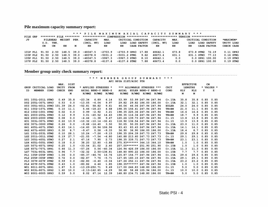
Pile maximum capacity summary report: ----------------------------------------------------------------------------------------------------------------------------------- * * * P I L E M A X I M U M A X I A L C A P A C I T Y S U M M A R Y * * * PILE GRP ********* PILE ********* ************** COMPRESSION ************* **************** TENSION *************** JT PILEHEAD WEIGHT PEN. CAPACITY MAX. CRITICAL CONDITION CAPACITY MAX. CRITICAL CONDITION *MAXIMUM* O.D. THK. (INCL. WT) LOAD LOAD LOAD SAFETY (INCL. WT) LOAD LOAD LOAD SAFETY UNITY LOAD CM CM KN M KN KN KN CASE FACTOR KN KN KN CASE FACTOR CHECK CASE 101P PL1 91.50 2.50 148.5 39.0 -48347.5 -2703.9 -2703.9 OPR3 17.88 48642.1 673.8 673.8 STM2 72.19 0.11 OPR3 103P PL2 91.50 2.50 148.5 39.0 -48378.8 -5031.2 -5031.2 STM1 9.62 48673.4 631.1 631.1 STM3 77.13 0.16 STM1 105P PL1 91.50 2.50 148.5 39.0 -48347.5 -5967.3 -5967.3 STM3 8.10 48642.1 0.0 0.0 OPR1 100.00 0.19 STM3 107P PL2 91.50 2.50 148.5 39.0 -48378.8 -6137.6 -6137.6 STM2 7.88 48673.4 0.0 0.0 OPR1 100.00 0.19 STM2 -------------------------------------------------------------------------------------------------------------------------------------
Member group unity check summary report: ----------------------------------------------------------------------------------------------------------------------------------- * * * M E M B E R G R O U P S U M M A R Y * * * API RP2A 21ST/AISC 9TH MAX. DIST EFFECTIVE CM GRUP CRITICAL LOAD UNITY FROM * APPLIED STRESSES * *** ALLOWABLE STRESSES *** CRIT LENGTHS * VALUES * ID MEMBER COND CHECK END AXIAL BEND-Y BEND-Z AXIAL EULER BEND-Y BEND-Z COND KLY KLZ Y Z M N/MM2 N/MM2 N/MM2 N/MM2 N/MM2 N/MM2 N/MM2 M M D01 105L-201L STM3 0.49 35.8 -23.34 6.89 6.14 53.99 53.99 247.94 247.94 C>.15A 35.8 35.8 0.85 0.85 D02 205L-307L OPR3 0.53 0.0 -13.05 -6.04 9.97 29.82 29.82 186.00 186.00 C>.15A 32.1 32.1 0.85 0.85 D03 305L-401L STM3 101.39 24.0 -52.81 58.82 9.61 46.06 46.06 247.94 247.94 EULER 24.0 24.0 0.85 0.85 H11 1002-107L STM1 0.10 11.1 5.46 -18.23 4.68 198.35 156.41 247.94 247.94 TN+BN 21.0 11.1 0.85 0.85 H12 1002-1001 STM2 0.02 0.0 0.99 -2.92 3.21 198.35 225.36 247.94 247.94 TN+BN 16.6 16.6 0.85 0.85 H21 2003-205L STM3 0.12 9.9 3.01 -20.52 14.43 198.35 116.34 247.94 247.94 TN+BN 18.7 9.9 0.85 0.85 H22 2003-2000 STM2 0.08 0.0 -4.44 -1.38 9.47 120.26 139.73 247.94 247.94 C<.15 13.8 13.8 0.85 0.85 H31 303L-307L STM3 0.22 13.9 -10.32 -10.14 -32.41 118.92 136.54 247.94 247.94 C<.15 13.9 13.9 0.85 0.85 H32 307L-3000 STM2 0.26 0.0 -9.68 -16.40 3.50 50.05 50.05 247.94 247.94 C>.15A 23.0 11.0 0.85 0.85 H41 405L-407L STM3 0.63 14.1 -14.60 18.94 106.96 83.43 83.43 247.94 247.94 C>.15A 14.1 14.1 0.85 0.85 H42 407L-4000 OPR3 0.30 8.7 -9.47 0.58 -9.33 36.90 36.90 186.00 186.00 C>.15A 18.4 8.7 0.85 0.85 LG1 103L-203L STM2 0.10 28.1 10.24 -7.26 -9.15 198.35 204.39 247.73 247.73 TN+BN 29.8 29.8 0.85 0.85 LG2 201L-301L STM2 0.19 27.7 -21.05 -7.54 -6.80 140.88 213.60 247.73 247.73 C<.15 29.1 29.1 0.85 0.85 LG3 305L-405L STM3 0.27 2.1 47.16 7.90 2.73 198.35 339.71 247.73 247.73 TN+BN 23.1 23.1 0.85 0.85 LG4 405L-505L STM3 0.18 0.0 38.20 12.80 -3.88 275.93******* 344.10 344.10 TN+BN 1.0 1.0 0.85 0.85 LG5 507L-607L OPR2 0.25 1.0 -33.54 21.02 2.40 207.00******* 251.90 251.90 C>.15B 1.0 1.0 0.85 0.85 LG6 607L-707L OPR1 0.66 11.3 -57.26 0.56 -40.34 126.94 426.09 186.00 186.00 C>.15A 11.3 11.3 0.85 0.85 LG7 703L-803L OPR1 0.96 7.7 -32.32 2.50-138.81 148.80 890.22 186.00 186.00 C>.15B 7.7 7.7 0.85 0.85 PL1 105P-205P STM3 1.06 0.0 -85.37 -46.76 16.76 125.87 154.77 247.94 247.94 C>.15A 29.6 29.6 0.85 0.85 PL2 205P-305P STM3 0.72 0.0 -82.87 7.76 -5.71 127.65 160.15 247.94 247.94 C>.15A 29.1 29.1 0.85 0.85 PL3 307P-407P STM2 0.59 0.0 -82.80 -6.40 -0.04 147.26 252.11 247.94 247.94 C>.15A 23.2 23.2 0.85 0.85 PL4 407P-507L STM2 0.43 1.0 -80.82 4.46 1.85 198.35******* 247.94 247.94 C>.15B 1.0 1.0 0.85 0.85 W01 8011-807L OPR1 1.87 5.0 -13.29-250.71 9.49 117.00 246.83 148.80 186.00 C<.15 5.0 5.0 0.85 0.85 W02 803L-807L OPR2 1.60 10.0 -2.13-162.85 -4.29 58.68 58.68 105.94 186.00 C<.15 10.0 10.0 0.85 0.85 W03 8001-8005 OPR3 0.59 5.0 8.02 67.14 12.39 148.80 234.71 148.80 186.00 TN+BN 5.0 5.0 0.85 0.85 -------------------------------------------------------------------------------------------------------------------------------------

Spectral Fatigue - 1
Part 8 -Spectral Fatigue Preparation
1) Under “Training Project”, create “Spectral Fatigue” subdirectory 2) Under “Spectral Fatigue”, Create “Foundation SE”, “Modes” and “Fatigue”
subdirectories. 3) Copy SACINP.STA model file, SEAINP.STA Seastate file and PSIINP.DAT soil data
from “\Spectral Earthquake\Static SE” directory to “Foundation SE” directory. 4) Copy SEAINP.DYN from “\Spectral Earthquake\Modes” directory to “Modes” directory
Creating foundation superelement under “Foundation SE” directory,
1) Modifying Model file SACINP.STA for creating foundation superelement suitable for wave response analysis
Live weight factor in weight combination MASS shall be modified from 0.75 to 1.0.
2) Modifying Seastate file SEAINP.STA for create foundation superelement suitable for
wave response analysis
Delete load conditions GRVX and GRVY; Add two new load conditions named as X000 and Y090, wave loads will be generated for 1.5 m wave height at 4.42 sec wave period for both 000 and 090 directions respectively. Stream function will be used for calculating wave force in 18 steps, maximum base shear will be selected for critical position. Weight selection lines INCWGT used to select weight groups ANOD and WKWY for possible wave forces. Delete load combination EQKS. Combine load combinations SUPX and SUPY with X000 and Y090 correspondingly. Modify LCSEL line to only include SUPX and SUPY load combinations.
Part of Seastate input file defined shall looks like following: ------------------------------------------------------------------------------------------------------------- LDOPT NF+Z 1.025 7.85 -79.50 79.50 MN NPNP K LCSEL SUPX SUPY … LOAD LOADCNDEAD INCWGT ANODWKWY DEAD DEAD -Z M LOADCNMASS INCWGT MASS ACCEL 1.0 N CEN1 LOADCNX000 INCWGT ANODWKWY
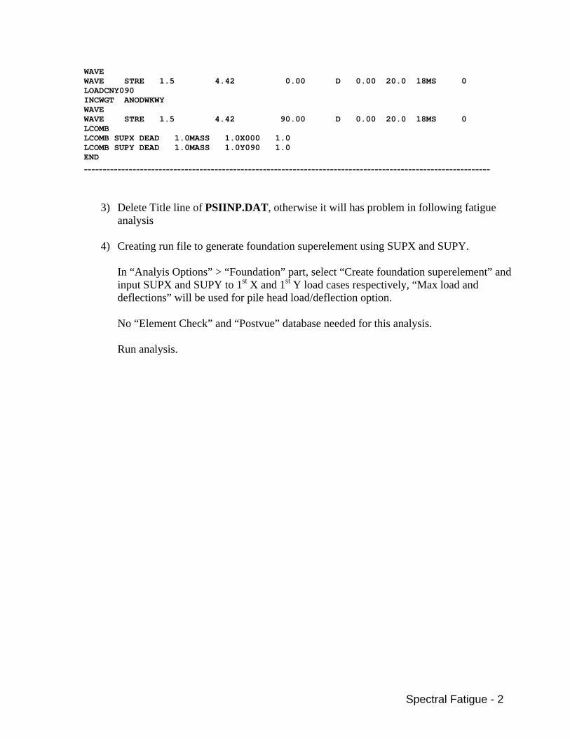
Spectral Fatigue - 2
WAVE WAVE STRE 1.5 4.42 0.00 D 0.00 20.0 18MS 0 LOADCNY090 INCWGT ANODWKWY WAVE WAVE STRE 1.5 4.42 90.00 D 0.00 20.0 18MS 0 LCOMB LCOMB SUPX DEAD 1.0MASS 1.0X000 1.0 LCOMB SUPY DEAD 1.0MASS 1.0Y090 1.0 END
-------------------------------------------------------------------------------------------------------------
3) Delete Title line of PSIINP.DAT, otherwise it will has problem in following fatigue analysis
4) Creating run file to generate foundation superelement using SUPX and SUPY.
In “Analyis Options” > “Foundation” part, select “Create foundation superelement” and input SUPX and SUPY to 1st X and 1st Y load cases respectively, “Max load and deflections” will be used for pile head load/deflection option. No “Element Check” and “Postvue” database needed for this analysis. Run analysis.

Spectral Fatigue - 3
Seastate basic load case summary report for spectral fatigue: ----------------------------------------------------------------------------------------------------------------------------------- ****** SEASTATE BASIC LOAD CASE SUMMARY ****** RELATIVE TO MUDLINE ELEVATION LOAD LOAD FX FY FZ MX MY MZ DEAD LOAD BUOYANCY CASE LABEL (KN) (KN) (KN) (KN-M) (KN-M) (KN-M) (KN) (KN) 1 DEAD 0.000 0.000 -5732.595 -30.701 10816.892 0.000 8601.126 2868.558 2 MASS 0.000 0.000 -5493.467 -558.857 8180.357 0.000 0.000 0.000 3 X000 5.435 -0.047 0.984 4.054 445.994 7.828 0.000 0.000 4 Y090 -0.538 25.079 1.352 -1862.846 -43.587 -20.975 0.000 0.000 -------------------------------------------------------------------------------------------------------------------------------------
Seastate combined load case summary report for spectral fatigue: ----------------------------------------------------------------------------------------------------------------------------------- ***** SEASTATE COMBINED LOAD CASE SUMMARY ***** RELATIVE TO MUDLINE ELEVATION LOAD LOAD FX FY FZ MX MY MZ CASE LABEL (KN) (KN) (KN) (KN-M) (KN-M) (KN-M) 5 SUPX 5.435 -0.047 -11225.078 -585.504 19443.244 7.828 6 SUPY -0.538 25.079 -11224.711 -2452.404 18953.664 -20.975 -------------------------------------------------------------------------------------------------------------------------------------
Pile head superelement created for joint 101P for spectral fatigue: ----------------------------------------------------------------------------------------------------------------------------------- *** PILEHEAD STIFFNESS FOR JOINT 101P *** FOR SUPERELEMENT NO. 1 RX RY RZ DX DY DZ RX 0.352555E+10 0.402477E+05 -0.402477E+04 0.329971E+02 0.122928E+08 -0.122928E+07 RY 0.402477E+05 0.349139E+10 -0.344714E+09 -0.122925E+08 -0.326704E+02 0.326704E+01 RZ -0.402477E+04 -0.344714E+09 0.787252E+08 0.122925E+07 0.326704E+01 -0.326704E+00 DX 0.329971E+02 -0.122925E+08 0.122925E+07 0.756676E+05 -0.864001E+00 0.864001E-01 DY 0.122928E+08 -0.326704E+02 0.326704E+01 -0.864001E+00 0.140090E+06 0.644293E+06 DZ -0.122928E+07 0.326704E+01 -0.326704E+00 0.864001E-01 0.644293E+06 0.651859E+07-------------------------------------------------------------------------------------------------------------------------------------

Spectral Fatigue - 4
Mode extraction under “Modes” directory,
Create Dynapac run file “Extract Mode Shapes”
Under “Analysis Options” > “Super Element”, select “Import Superelement” and browse in “Foundation SE” directory for DYNSEF.STA file. Under “Analysis Options” > “Mode Shape”, choose “Use Modal Extraction Options”; input 50 to “Number of Modes” and select “Create added mass of beams”. Choose “Seastate” options and create “Postvue” database. Browse in “Foundation SE” directory for SACINP.STA when prompted for “Model Data file”. Run Analysis.
Spectral Fatigue - 5
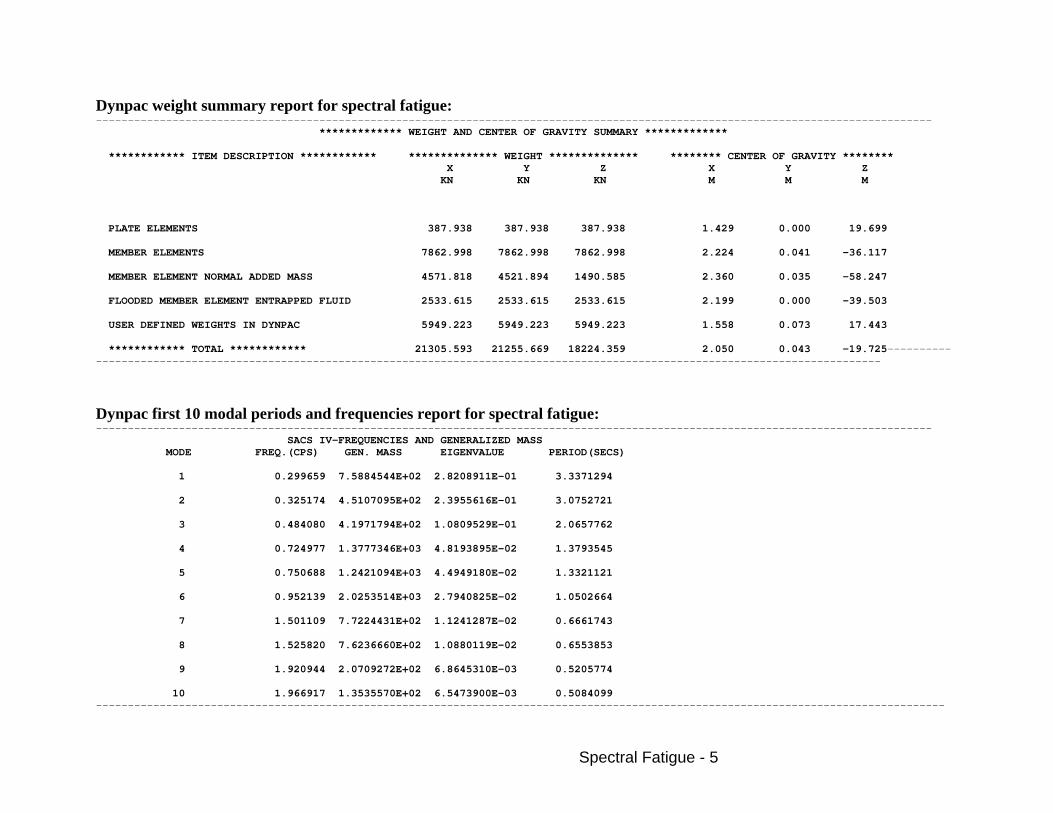
Dynpac weight summary report for spectral fatigue: ----------------------------------------------------------------------------------------------------------------------------------- ************* WEIGHT AND CENTER OF GRAVITY SUMMARY ************* ************ ITEM DESCRIPTION ************ ************** WEIGHT ************** ******** CENTER OF GRAVITY ******** X Y Z X Y Z KN KN KN M M M PLATE ELEMENTS 387.938 387.938 387.938 1.429 0.000 19.699 MEMBER ELEMENTS 7862.998 7862.998 7862.998 2.224 0.041 -36.117 MEMBER ELEMENT NORMAL ADDED MASS 4571.818 4521.894 1490.585 2.360 0.035 -58.247 FLOODED MEMBER ELEMENT ENTRAPPED FLUID 2533.615 2533.615 2533.615 2.199 0.000 -39.503 USER DEFINED WEIGHTS IN DYNPAC 5949.223 5949.223 5949.223 1.558 0.073 17.443 ************ TOTAL ************ 21305.593 21255.669 18224.359 2.050 0.043 -19.725-------------------------------------------------------------------------------------------------------------------------------------
Dynpac first 10 modal periods and frequencies report for spectral fatigue: ----------------------------------------------------------------------------------------------------------------------------------- SACS IV-FREQUENCIES AND GENERALIZED MASS MODE FREQ.(CPS) GEN. MASS EIGENVALUE PERIOD(SECS) 1 0.299659 7.5884544E+02 2.8208911E-01 3.3371294 2 0.325174 4.5107095E+02 2.3955616E-01 3.0752721 3 0.484080 4.1971794E+02 1.0809529E-01 2.0657762 4 0.724977 1.3777346E+03 4.8193895E-02 1.3793545 5 0.750688 1.2421094E+03 4.4949180E-02 1.3321121 6 0.952139 2.0253514E+03 2.7940825E-02 1.0502664 7 1.501109 7.7224431E+02 1.1241287E-02 0.6661743 8 1.525820 7.6236660E+02 1.0880119E-02 0.6553853 9 1.920944 2.0709272E+02 6.8645310E-03 0.5205774 10 1.966917 1.3535570E+02 6.5473900E-03 0.5084099 -------------------------------------------------------------------------------------------------------------------------------------

Spectral Fatigue - 6
Wave Response analysis under “Fatigue” directory,
1) Create Seastate input file SEAINP.000, SEAINP.045 and SEAINP.090 for Transfer function generation
Copy SEAINP.DYN Seastate file from “Modes” directory and rename to SEAINP.000. Input DYN analysis option in col.56-58 for generating loading and hydrodynamic modeling for dynamics. Input title line as “000 DIRECTION TRANSFER FUNCTION”. Four load cases 1 through 4 will be added, each load case contain one line of GNTRF transfer function generation line. For fist load case in 000 direction: 6 waves in 18 steps will be generated using wave steepness 0.05; beginning wave period 10 seconds and period step size 1.00 seconds; transfer function loading will be generated for each wave position and AIRY wave theory will be selected. Base shear and overturning moment will be plotted
For second load case in 000 direction, 6 waves with starting period = 4.75 secs and period step size = 0.25 secs. For third load case in 000 direction, 11 waves with starting period = 3.40 secs and period step size = 0.10 secs. For fourth load case in 000 direction, 2 waves with starting period = 2.25 secs and period step size = 0.25 secs. Copy SEAINP.000 Seastate file to SEAINP.045 and SEAINP.090. Modify GNTRF directions to 45.00 for SEAINP.045 and to 90.00 for SEAINP.090.
Part of Seastate input file defined for 000 direction shall looks like following: ------------------------------------------------------------------------------------------------------------- LDOPT NF+Z 1.025 7.85 -79.50 79.50 MN DYN NPNP K 000 DIRECTION TRANSFER FUNCTION FILE S … LOAD LOADCN 1 GNTRF AL 6 0.05 10.00 1.00 0.00 18AIRYPF LOADCN 2 GNTRF AL 6 0.05 4.75 0.25 0.00 18AIRYPF LOADCN 3 GNTRF AL 11 0.05 3.40 0.10 0.00 18AIRYPF LOADCN 4 GNTRF AL 2 0.05 2.25 0.25 0.00 18AIRYPF END
-------------------------------------------------------------------------------------------------------------

Spectral Fatigue - 7
2) Create wave response input file WVRINP.PLT for transfer function plot
For Wave Response Options, select “ALL” to Load case selection, choose “Generate Plots”, maximum allowable iterations = -1. Use Transfer function plot line PLTTF to request Overturning moment and Base shear plot for both period and frequency. 1 to 25 load case selected for transfer function load case TFLCAS. Damping ratio for spectral fatigue use 2% for all modes.
Wave response plot input file defined shall looks like following: ------------------------------------------------------------------------------------------------------------- WROPT MNPSL ALL -1 PLTTF OM BS PFS TFLCAS 1 25 DAMP 2.0 END
-------------------------------------------------------------------------------------------------------------
3) Create wave response run file and creating transfer function plot for 000 direction Under “Analysis Options” > “Wave Response”, make sure WVRINP.PLT is in Wave Response input file filed. Under “Analysis Options” > “Seastate”, check “Execute Seastate” and “Seastate file not in model file” and browse for SEAINP.000. Browse to “Foundation SE” directory for model data file SACINP.STA, and browse to “Modes” directory for mode and mass file. Run the analysis and study the generated plots.
4) Creating wave response input file WVRINP.EQS for equivalent loads generation
Copy WVRINP.PLT to WVRINP.EQS, in wave options line, select “ES – Equivalent Static Loads”.
Wave response input file for equivalent loads defined shall looks like following: ------------------------------------------------------------------------------------------------------------- WROPT MNPSL ALL ES -1 PLTTF OM BS PFS TFLCAS 1 25 DAMP 2.0 END
-------------------------------------------------------------------------------------------------------------
Spectral Fatigue - 8
5) Creating and solving equivalent loads for 000 direction
Under “Analysis Options” > “Wave Response”, browse for “WVRINP.EQS”. Under “Analysis Options” > “Seastate”, select “Execute Seastate” and check “Seastate input not in model file”, make sure SEAINP.000 appears in the Seastate input file window. Start Wizard begin generating wave response run file. When “Analysis Options” reappears, under “Wave Response” window, select “Solving equivalent static loads automatically”. Then under “Foundation”, check “Use non-linear foundation” and browse to “Foundation SE” directory for PSIINP.DAT file. Choose “Create pile fatigue solution file” for Pile Fatigue Solution File Option. Browse to “Foundation SE” for model data file SACINP.STA. Browse to “Modes” for mode and mass file. Run Analysis.
6) Use the same procedure as 5) and solving equivalent loads for 045 and 090 directions. 7) Create fatigue input file FTGINP.FTG for spectral fatigue analysis
For fatigue options, Number of Additional Postfiles = 2 Design life = 20 yrs Fatigue Time Period = 1.0 yrs
Check “Skip Non-Tubular Elements”, “Use Load Case Dependent SCF’s”, “Prescribe Max SCF” and “Prescribe MIN SCF” Choose API X prime curve for S-N Curve and Efthymiou method EFT for SCF calculation
For fatigue option 2 line, check “Member Summ. Rep. (Life Order)” and “SCF Validity Range Check”. Using joint override lines JNTOVR to define that joints 401L, 403L, 405L and 407L will be checked using API X curve rather than X prime curve. Using group selection line GRPSEL to remove member groups PL1, PL2, PL3, PL4 and W.B from fatigue calculation. Using joint selection JSLC line to define only joints 201L, 203L, 205L, 207L, 301L, 303L, 305L, 307L, 401L, 403L, 405L and 407L will be included for fatigue damage evaluations.
Spectral Fatigue - 9
Using SCF limits line SCFLM to define max. SCF = 6.0 and min. SCF = 1.5. SCF Selection line SCFSEL can be used to define for X type joints, Marshall method MSH will be used for SCF calculation. Add a RELIEF to force the program to evaluate the member hot spot stress at the surface of chord. SEAS line will be used to signal the program to read the Seastate input data file to determine the SACS load case to wave period and direction correlation. Input first fatigue load case corresponding to direction 000
Using Spectral Wave Fatigue Case FTLOAD to input Fraction of Design Life = 0.47 for 000 direction; input “SPC” into column 32-34 for spectral fatigue case. Using Scatter Diagram Header SCATD to select Pierson-Moskowitz Spectrum as type of wave spectrum. Using Scatter Diagram Wave height SCWAV to input sea states wave heights and using Scatter Diagram Freq. of Occurrence SCPER line to input Frequency of Occurrence per wave period. Percent occurrence for various wave heights and wave periods for 000 direction:
Significant Wave Height (M) Dominant Period (SECS)
0.0 - 0.6 0.6 – 1.4 1.4 – 2.6
1.0 – 2.0 0.15 0.10 0.10
2.0 – 4.0 0.10 0.19 0.11
4.0 – 6.0 0.05 0.08 0.05
6.0 – 10.0 0.02 0.03 0.02
Input second fatigue load case corresponding to direction 045
Using Spectral Wave Fatigue Case FTLOAD to input Fraction of Design Life = 0.2 for 045 direction; input “SPC” into column 32-34 for spectral fatigue case. Percent occurrence for various wave heights and wave periods for 045 direction:

Spectral Fatigue - 10
Significant Wave Height (M) Dominant Period (SECS)
0.0 - 0.6 0.6 – 1.4 1.4 – 2.6
1.0 – 2.0 0.10 0.13 0.08
2.0 – 4.0 0.15 0.13 0.10
4.0 – 6.0 0.08 0.08 0.07
6.0 – 10.0 0.03 0.02 0.03
Input third fatigue load case corresponding to direction 090
Using Spectral Wave Fatigue Case FTLOAD to input Fraction of Design Life = 0.33 for 090 direction; input “SPC” into column 32-34 for spectral fatigue case. Percent occurrence for various wave heights and wave periods for 090 direction:
Significant Wave Height (M) Dominant Period (SECS)
0.0 - 0.6 0.6 – 1.4 1.4 – 2.6
1.0 – 2.0 0.13 0.10 0.08
2.0 – 4.0 0.13 0.15 0.10
4.0 – 6.0 0.06 0.09 0.08
6.0 – 10.0 0.03 0.03 0.02
Using Joint Extraction Head EXTRAC line to extract all joints with damage level greater than 0.5 for Interactive Fatigue review.
Fatigue input file defined shall looks like following: ------------------------------------------------------------------------------------------------------------- FATGIUE INPUT FTOPT 2 20. 1.0 2. SMAPP MXMNSK LPEFT FTOPT2 PTVC JNTOVR 401L API JNTOVR 403L API

Spectral Fatigue - 11
JNTOVR 405L API JNTOVR 407L API GRPSEL RM PL1 PL2 PL3 PL4 W.B JSLC 201L203L205L207L301L303L305L307L401L403L405L407L SCFLM 6.0 1.5 SCFSEL MSH RELIEF SEAS FTLOAD 1 .47 1.0 SPC SCATD D 1.0 1.0 PM SCWAV 0.30 1.0 2.0 SCPER 1.5 .15 .1 .1 SCPER 3.0 .1 .19 .11 SCPER 5.0 .05 .08 .05 SCPER 8.0 .02 .03 .02 FTLOAD 2 .20 1.0 SPC SCATD D 1.0 1.0 PM SCWAV 0.30 1.0 2.0 SCPER 1.5 .10 .13 .08 SCPER 3.0 .15 .13 .10 SCPER 5.0 .08 .08 .07 SCPER 8.0 .03 .02 .03 FTLOAD 3 .33 1.0 SPC SCATD D 1.0 1.0 PM SCWAV 0.30 1.0 2.0 SCPER 1.5 .13 .10 .08 SCPER 3.0 .13 .15 .10 SCPER 5.0 .06 .09 .08 SCPER 8.0 .03 .03 .02 EXTRAC HEAD AE 0.5 END
-------------------------------------------------------------------------------------------------------------
8) Create fatigue run file and run the analysis. Browse for results and using interactive fatigue to review critical joints.

Spectral Fatigue - 12
Portion of spectral fatigue analysis report for joint 407L and 403L: ----------------------------------------------------------------------------------------------------------------------------------- * * * M E M B E R F A T I G U E R E P O R T * * * (DAMAGE ORDER) ORIGINAL CHORD REQUIRED JOINT MEMBER GRUP TYPE OD WT JNT MEM LEN. GAP * STRESS CONC. FACTORS * FATIGUE RESULTS OD WT ID ID (CM) (CM) TYP TYP (M ) (CM) AX-CR AX-SD IN-PL OU-PL DAMAGE LOC SVC LIFE (CM) (CM) 407L 403L-407L H41 TUB 32.38 1.250 Y BRC 12.12 0.00 3.00 6.00 2.35 3.53 5.271789 BL 3.793778 407L 407L-507L LG4 TUB 107.00 3.500 Y CHD 12.12 2.53 4.74 1.59 2.74 1.382290 BL 14.46874 407L 405L-407L H41 TUB 32.38 1.250 Y BRC 12.12 0.00 3.00 6.00 2.35 3.53 1.882799 BR 10.62249 407L 407L-507L LG4 TUB 107.00 3.500 Y CHD 12.12 2.53 4.74 1.59 2.74 .4480346 BR 44.63941 407L 407L-4000 H42 TUB 32.38 1.250 Y BRC 12.12 0.00 3.00 6.00 2.35 3.51 .5309010 BR 37.67181 407L 407L-507L LG4 TUB 107.00 3.500 Y CHD 12.12 2.53 4.71 1.58 2.72 .1215998 BR 164.4740 ---------------------------------------------------------------------------------------------------------------------------------- 403L 307L-403L D03 TUB 40.75 1.500 K BRC 12.12 30.96 2.68 2.62 2.78 2.09 .3926162 T 50.94033 403L 303L-403L LG3 TUB 107.00 3.500 K CHD 12.12 2.69 2.74 1.50 1.86 .1846078 TL 108.3378 403L 401L-403L H41 TUB 32.38 1.250 Y BRC 12.12 0.00 3.00 6.00 2.35 3.53 1.836187 BL 10.89213 403L 403L-503L LG4 TUB 107.00 3.500 Y CHD 12.12 2.53 4.74 1.59 2.74 .4494944 BL 44.49443 403L 403L-407L H41 TUB 32.38 1.250 K BRC 12.12 30.96 3.93 5.25 2.35 3.57 5.087764 TL 3.931000 403L 403L-503L LG4 TUB 107.00 3.500 K CHD 12.12 3.33 4.29 1.59 2.77 1.428185 TL 14.00379 403L 403L-4000 H42 TUB 32.38 1.250 Y BRC 12.12 0.00 3.00 6.00 2.35 3.51 .1326569 BL 150.7648 403L 403L-503L LG4 TUB 107.00 3.500 Y CHD 12.12 2.53 4.71 1.58 2.72 .0221272 BL 903.8660 -------------------------------------------------------------------------------------------------------------------------------------

Spectral Fatigue - 13
9) Foundation pile fatigue analysis
Copy FTGINP.FTG to FTGINP.PIL, delete unrelated lines for pile fatigue analysis. JNTOVR, GRPSEL, JSLC, SCFSEL, RELIEF and EXTRAC line(s) will be deleted. Modify fatigue option line 2 and check “Tubular Inline Check”, chose American Welding Society S-N curve AWS for pile fatigue analysis. Modifying SCF limits line, Max. SCF =1.5 and Min. SCF = 1.0.
Pile Fatigue input file defined shall looks like following: ------------------------------------------------------------------------------------------------------------- FOUNDATION PILE FATIGUE INPUT FTOPT 2 20. 1.0 2. SMAPP MXMNSK LPEFT FTOPT2 PTVC AWS TI2 SCFLM 1.5 1.0 SEAS FTLOAD 1 .47 1.0 SPC SCATD D 1.0 1.0 PM SCWAV 0.30 1.0 2.0 SCPER 1.5 .15 .1 .1 SCPER 3.0 .1 .19 .11 SCPER 5.0 .05 .08 .05 SCPER 8.0 .02 .03 .02 FTLOAD 2 .20 1.0 SPC SCATD D 1.0 1.0 PM SCWAV 0.30 1.0 2.0 SCPER 1.5 .10 .13 .08 SCPER 3.0 .15 .13 .10 SCPER 5.0 .08 .08 .07 SCPER 8.0 .03 .02 .03 FTLOAD 3 .33 1.0 SPC SCATD D 1.0 1.0 PM SCWAV 0.30 1.0 2.0 SCPER 1.5 .13 .10 .08 SCPER 3.0 .13 .15 .10 SCPER 5.0 .06 .09 .08 SCPER 8.0 .03 .03 .02 END
------------------------------------------------------------------------------------------------------------- Create fatigue run file and run the analysis. Browse for results.
Spectral Fatigue - 14
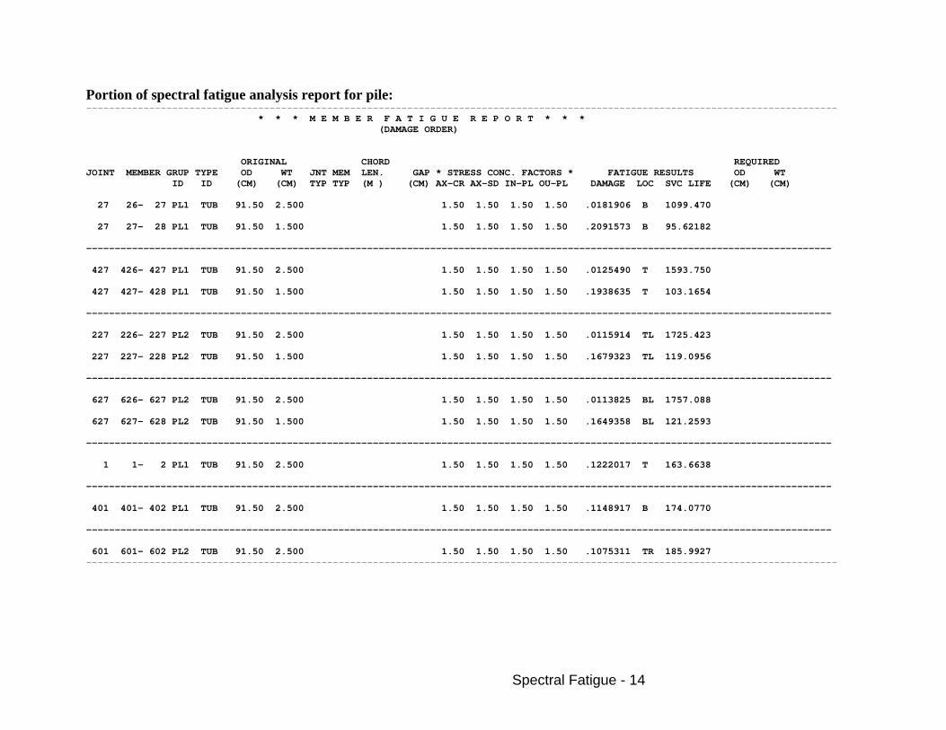
Portion of spectral fatigue analysis report for pile: ----------------------------------------------------------------------------------------------------------------------------------- * * * M E M B E R F A T I G U E R E P O R T * * * (DAMAGE ORDER) ORIGINAL CHORD REQUIRED JOINT MEMBER GRUP TYPE OD WT JNT MEM LEN. GAP * STRESS CONC. FACTORS * FATIGUE RESULTS OD WT ID ID (CM) (CM) TYP TYP (M ) (CM) AX-CR AX-SD IN-PL OU-PL DAMAGE LOC SVC LIFE (CM) (CM) 27 26- 27 PL1 TUB 91.50 2.500 1.50 1.50 1.50 1.50 .0181906 B 1099.470 27 27- 28 PL1 TUB 91.50 1.500 1.50 1.50 1.50 1.50 .2091573 B 95.62182 ---------------------------------------------------------------------------------------------------------------------------------- 427 426- 427 PL1 TUB 91.50 2.500 1.50 1.50 1.50 1.50 .0125490 T 1593.750 427 427- 428 PL1 TUB 91.50 1.500 1.50 1.50 1.50 1.50 .1938635 T 103.1654 ---------------------------------------------------------------------------------------------------------------------------------- 227 226- 227 PL2 TUB 91.50 2.500 1.50 1.50 1.50 1.50 .0115914 TL 1725.423 227 227- 228 PL2 TUB 91.50 1.500 1.50 1.50 1.50 1.50 .1679323 TL 119.0956 ---------------------------------------------------------------------------------------------------------------------------------- 627 626- 627 PL2 TUB 91.50 2.500 1.50 1.50 1.50 1.50 .0113825 BL 1757.088 627 627- 628 PL2 TUB 91.50 1.500 1.50 1.50 1.50 1.50 .1649358 BL 121.2593 ---------------------------------------------------------------------------------------------------------------------------------- 1 1- 2 PL1 TUB 91.50 2.500 1.50 1.50 1.50 1.50 .1222017 T 163.6638 ---------------------------------------------------------------------------------------------------------------------------------- 401 401- 402 PL1 TUB 91.50 2.500 1.50 1.50 1.50 1.50 .1148917 B 174.0770 ---------------------------------------------------------------------------------------------------------------------------------- 601 601- 602 PL2 TUB 91.50 2.500 1.50 1.50 1.50 1.50 .1075311 TR 185.9927 -----------------------------------------------------------------------------------------------------------------------------------

Extreme Wave - 1
Part 10 -Extreme Wave Preparation
1) Under “Training Project”, create “Extreme Wave” subdirectory 2) Under “Extreme Wave”, Create “Foundation SE”, “Modes” and “Dynamic Wave”
subdirectories. 3) Copy SACINP.STA model file, SEAINP.STA and PSIINP.DAT soil data from “\Spectral
Earthquake\Static SE” directory to “Foundation SE” directory.
Creating foundation superelement under “Foundation SE” directory,
1) Modifying Seastate file SEAINP.STA
Delete EQKS from LCSEL and load combinations. Delete load conditions GRVX and GRVY, add two new load conditions named as X000 and Y090, wave loads will be generated for 5.5 m wave height at 8.00 sec wave period for both 000 and 090 directions respectively. Stream function will be used for calculating wave force in 18 steps, maximum base shear will be selected for critical position. Still water depth override 80 m will be used for wave load generation. Associated current will be added to each of these load cases. Current velocity used 0.207 m/s at bottom and 0.900 m/s at surface; Linear stretch will be used and apparent wave period will be calculated; Automatic blocking factor will be used at elevation -5.0 m. Weight group selection INCWGT line for ANOD and WKWY will be added to each of these two wave cases for possible environmental loadings. In load combinations SUPX and SUPY using X000 to replace GRVX and Y090 to replace GRVY. Portion of modified Seastate input shall looks like following, ------------------------------------------------------------------------------------------------------------- LDOPT NF+Z 1.025 7.85 -79.50 79.50 MN NPNP K LCSEL SUPX SUPY … LOAD LOADCNDEAD INCWGT ANODWKWY DEAD DEAD -Z M LOADCNMASS INCWGT MASS ACCEL 1.0 N CEN1 LOADCNX000 INCWGT ANODWKWY CURR CURR 0.00 0.207 0.00 -5.0BC LN AWP CURR 79.50 0.900 0.00

Extreme Wave - 2
WAVE WAVE STRE 5.50 80.0 8.00 0.00 D 0.00 20.0 18MS 0 LOADCNY090 INCWGT ANODWKWY CURR CURR 0.00 0.207 90.00 -5.0BC LN AWP CURR 79.50 0.900 90.00 WAVE WAVE STRE 5.50 80.0 8.00 90.00 D 0.00 20.0 18MS 0 LCOMB LCOMB SUPX DEAD 1.0MASS 1.0X000 1.0 LCOMB SUPY DEAD 1.0MASS 1.0Y090 1.0 END
------------------------------------------------------------------------------------------------------------- 2) Creating run file to generate foundation superelement using SUPX and SUPY.
In “Analyis Options” > “Foundation” part, select “Create foundation superelement” and input SUPX and SUPY to 1st X and 1st Y load cases respectively, “Max load and deflections” will be used for pile head load/deflection option. No “Element Check” and “Postvue” database needed for this analysis. Run analysis.
Mode extraction under “Modes” directory,
1) Copy Seastate SEAINP.DYN file from “\Spectral Earthquake\Modes” directory to “Modes” directory.
2) Create Dynapac run file “Extract Mode Shapes”
Under “Analysis Options” > “Super Element”, select “Import Superelement” and browse in “Foundation SE” directory for DYNSEF.STA file. Under “Analysis Options” > “Mode Shape”, choose “Use Modal Extraction Options”; input 50 to “Number of Modes” and select “Create added mass of beams”. Choose “Seastate” options and create “Postvue” database. Browse in “Foundation SE” directory for SACINP.STA when prompted for “Model Data file”. Run Analysis.
Extreme Wave Response analysis under “Dynamic Wave” directory,
1) Create Seastate SEAINP.EXW to define environmental load cases

Extreme Wave - 3
Copy SEAINP.STA from “Foundation SE” to “Dynamic Wave” directory and rename to SEAINP.EXW. Rename load conditions X000 to E000, Y090 to E090. Change wave from 5.5 m @ 8.0 sec to 3.5 m @ 5.0 sec. Wind load will be added for 45.17 m/s, water depth override = 80.0 m and AP08 will be used for wind profile. Make copy of load case E000 to E045, change corresponding directions as necessary. Change load combinations SUPX and SUPY to CMB1 and CMB3 corresponding to E000 and E090. Add load combination CMB2 corresponding to E045. Chang load case selection to select CMB1, CMB2 and CMB3. Create loading and hydrodynamic modeling for dynamics option “DYN” on load options line will be defined at col. 56-58. Portion of modified Seastate input shall looks like following, ------------------------------------------------------------------------------------------------------------- LDOPT NF+Z 1.025 7.85 -79.50 79.50 MN DYN NPNP K LCSEL CMB1 CMB2 CMB3 … LOAD LOADCNDEAD INCWGT ANODWKWY DEAD DEAD -Z M LOADCNMASS INCWGT MASS ACCEL 1.0 N CEN1 LOADCNE000 INCWGT ANODWKWY WIND WIND 45.17 0.00 80.0AP08 CURR CURR 0.00 0.207 0.00 -5.0BC LN AWP CURR 79.50 0.900 0.00 WAVE WAVE STRE 3.50 80.0 5.00 0.00 D 0.00 20.0 18MS 0 LOADCNE045 INCWGT ANODWKWY WIND WIND 45.17 45.00 80.0AP08 CURR CURR 0.00 0.207 45.00 -5.0BC LN AWP CURR 79.50 0.900 45.00 WAVE WAVE STRE 3.50 80.0 5.00 45.00 D 0.00 20.0 18MS 0 LOADCNE090 INCWGT ANODWKWY WIND WIND 45.17 90.00 80.0AP08

Extreme Wave - 4
CURR CURR 0.00 0.207 90.00 -5.0BC LN AWP CURR 79.50 0.900 90.00 WAVE WAVE STRE 3.50 80.0 5.00 90.00 D 0.00 20.0 18MS 0 LCOMB LCOMB CMB1 DEAD 1.0MASS 1.0E000 1.0 LCOMB CMB2 DEAD 1.0MASS 1.0E045 1.0 LCOMB CMB3 DEAD 1.0MASS 1.0E090 1.0 END
------------------------------------------------------------------------------------------------------------- 2) Create dynamic response input file DYRINP.EXW for this extreme wave analysis
Wave response options: MN unit will be used with Extreme wave equivalent static load generation corresponding to maximum base shear. Number of modes used = 50 and Maximum number of iterations = 10. Plot selection PSEL line will be used to select plots for Joint Displacement, Member force, Overturning moment and base shear. Joint plot selection PSJO is used to plot joint displacement, velocity and acceleration for joint 401L in X and Y directions. Member force plot selection PSMF is used to plot member axial force at member end B for member 303L-401L and 307L-403L. Structural damping 2%. Wave response input for extreme wave shall looks like following, ------------------------------------------------------------------------------------------------------------- WROPT MNPSL MAXSEX 50 10 PSEL JO MF OM BS PSJO 401LDX401LDY401LVX401LVY401LAX401LAY PSMF 303L401LFXB307L403LFXB DAMP 2.0 END
------------------------------------------------------------------------------------------------------------- 3) Run wave response analysis and solve the generated loads with non-linear foundations.
Browse in “Modes” directory for mode and mass file, browse in “Foundation SE” directory for model data file and soil data file. Run analysis. 4) Create post input file PSTINP.EXW for element code check
Using SACS options, select load case CMB1, CMB2 and CMB3 for element analysis; define AMOD = 1.333 for the selected load cases; a UCPART line may added. Post code check input file shall looks like following,

Extreme Wave - 5
------------------------------------------------------------------------------------------------------------- OPTION MN SDUC 2 1 PTPTPT PTPTPT LCSEL IN CMB1 CMB2 CMB3 UCPART 0.5 0.5 1.0 1.0300.0 AMOD CMB1 1.333CMB2 1.333CMB3 1.333 END
------------------------------------------------------------------------------------------------------------- Create post run file and run the analysis. Browse for results.
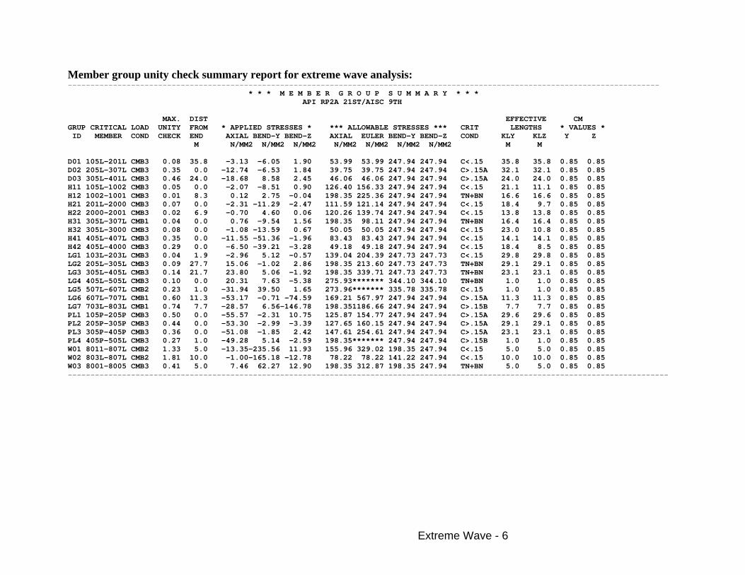
Extreme Wave - 6
Member group unity check summary report for extreme wave analysis: ----------------------------------------------------------------------------------------------------------------------------------- * * * M E M B E R G R O U P S U M M A R Y * * * API RP2A 21ST/AISC 9TH MAX. DIST EFFECTIVE CM GRUP CRITICAL LOAD UNITY FROM * APPLIED STRESSES * *** ALLOWABLE STRESSES *** CRIT LENGTHS * VALUES * ID MEMBER COND CHECK END AXIAL BEND-Y BEND-Z AXIAL EULER BEND-Y BEND-Z COND KLY KLZ Y Z M N/MM2 N/MM2 N/MM2 N/MM2 N/MM2 N/MM2 N/MM2 M M D01 105L-201L CMB3 0.08 35.8 -3.13 -6.05 1.90 53.99 53.99 247.94 247.94 C<.15 35.8 35.8 0.85 0.85 D02 205L-307L CMB3 0.35 0.0 -12.74 -6.53 1.84 39.75 39.75 247.94 247.94 C>.15A 32.1 32.1 0.85 0.85 D03 305L-401L CMB3 0.46 24.0 -18.68 8.58 2.45 46.06 46.06 247.94 247.94 C>.15A 24.0 24.0 0.85 0.85 H11 105L-1002 CMB3 0.05 0.0 -2.07 -8.51 0.90 126.40 156.33 247.94 247.94 C<.15 21.1 11.1 0.85 0.85 H12 1002-1001 CMB3 0.01 8.3 0.12 2.75 -0.04 198.35 225.36 247.94 247.94 TN+BN 16.6 16.6 0.85 0.85 H21 201L-2000 CMB3 0.07 0.0 -2.31 -11.29 -2.47 111.59 121.14 247.94 247.94 C<.15 18.4 9.7 0.85 0.85 H22 2000-2001 CMB3 0.02 6.9 -0.70 4.60 0.06 120.26 139.74 247.94 247.94 C<.15 13.8 13.8 0.85 0.85 H31 305L-307L CMB1 0.04 0.0 0.76 -9.54 1.56 198.35 98.11 247.94 247.94 TN+BN 16.4 16.4 0.85 0.85 H32 305L-3000 CMB3 0.08 0.0 -1.08 -13.59 0.67 50.05 50.05 247.94 247.94 C<.15 23.0 10.8 0.85 0.85 H41 405L-407L CMB3 0.35 0.0 -11.55 -51.36 -1.96 83.43 83.43 247.94 247.94 C<.15 14.1 14.1 0.85 0.85 H42 405L-4000 CMB3 0.29 0.0 -6.50 -39.21 -3.28 49.18 49.18 247.94 247.94 C<.15 18.4 8.5 0.85 0.85 LG1 103L-203L CMB3 0.04 1.9 -2.96 5.12 -0.57 139.04 204.39 247.73 247.73 C<.15 29.8 29.8 0.85 0.85 LG2 205L-305L CMB3 0.09 27.7 15.06 -1.02 2.86 198.35 213.60 247.73 247.73 TN+BN 29.1 29.1 0.85 0.85 LG3 305L-405L CMB3 0.14 21.7 23.80 5.06 -1.92 198.35 339.71 247.73 247.73 TN+BN 23.1 23.1 0.85 0.85 LG4 405L-505L CMB3 0.10 0.0 20.31 7.63 -5.38 275.93******* 344.10 344.10 TN+BN 1.0 1.0 0.85 0.85 LG5 507L-607L CMB2 0.23 1.0 -31.94 39.50 1.65 273.96******* 335.78 335.78 C<.15 1.0 1.0 0.85 0.85 LG6 607L-707L CMB1 0.60 11.3 -53.17 -0.71 -74.59 169.21 567.97 247.94 247.94 C>.15A 11.3 11.3 0.85 0.85 LG7 703L-803L CMB1 0.74 7.7 -28.57 6.56-146.78 198.351186.66 247.94 247.94 C>.15B 7.7 7.7 0.85 0.85 PL1 105P-205P CMB3 0.50 0.0 -55.57 -2.31 10.75 125.87 154.77 247.94 247.94 C>.15A 29.6 29.6 0.85 0.85 PL2 205P-305P CMB3 0.44 0.0 -53.30 -2.99 -3.39 127.65 160.15 247.94 247.94 C>.15A 29.1 29.1 0.85 0.85 PL3 305P-405P CMB3 0.36 0.0 -51.08 -1.85 2.42 147.61 254.61 247.94 247.94 C>.15A 23.1 23.1 0.85 0.85 PL4 405P-505L CMB3 0.27 1.0 -49.28 5.14 -2.59 198.35******* 247.94 247.94 C>.15B 1.0 1.0 0.85 0.85 W01 8011-807L CMB2 1.33 5.0 -13.35-235.56 11.93 155.96 329.02 198.35 247.94 C<.15 5.0 5.0 0.85 0.85 W02 803L-807L CMB2 1.81 10.0 -1.00-165.18 -12.78 78.22 78.22 141.22 247.94 C<.15 10.0 10.0 0.85 0.85 W03 8001-8005 CMB3 0.41 5.0 7.46 62.27 12.90 198.35 312.87 198.35 247.94 TN+BN 5.0 5.0 0.85 0.85 -------------------------------------------------------------------------------------------------------------------------------------

Gap Loadout - 1
Part 13 - Load out with no load gap elements Preparation
1) Under “Training Project”, create “Gap Loadout” subdirectory 2) Copy SACINP.DAT model file from “Static PSI” directory to “Gap Loadout” directory.
Modifying model to only include jacket for load out
Delete all weight definitions for deck structure. In Precede, delete deck structures, plates and plate groups, all piles and wishbones. Using “Display” > “Zoom Box” > “Translate/Rotate” > “General”, select the whole structure, pick rotation angle about Y, input rotation angle -90.0, input Z translation = 11.0 m to rotate and move the structure. Using “Display” > “Zoom Box” > “Translate/Rotate” > “General” again, select the whole structure, pick rotation angle about Z, input rotation angle 180.0. rotate the structure to final fabrication position.
Delete all Ky and Ly definitions. Add Kz and Lz definitions for jacket horizontal framings.
Add joints 1101, 1105, 1201, 1205, 1301, 1305, 1401 and 1405 relative to 101L, 105L, 201L, 205L, 301L, 305L, 401L and 405L correspondingly with dZ = -1.75;
Add joints 2101, 2105, 2201, 2205, 2301, 2305, 2401 and 2405 relative to 1101, 1105, 1201, 1205, 1301, 1305, 1401 and 1405 correspondingly with dZ = -1.75; Connecting these joints vertically with members using member group label set to CAN. Modifying members 2101-1101, 2105-1105, 2201-1201, 2205-1205, 2301-1301, 2305-1305, 2401-1401 and 2405-1405 to compression only members. Modifying members 1101-101L, 1105-105L, 1201-201L, 1205-205L, 1301-301L, 1305-305L, 1401-401L and 1405-405L to set joint B Z direction offsets -53.50 cm. Set joint fixity 001000 to joints 2101, 2105, 2201, 2205, 2301, 2305, 2401 and 2405. Set joint fixity 110000 to joints 1101, 1105, 1201, 1205, 1301, 1305, 1401 and 1405. Add member properties for CAN: Member group CAN, Diameter = 76.20 cm, Wall Thickness = 2.54 cm

Gap Loadout - 2
The added member group CAN, members and joints shall looks like following: ------------------------------------------------------------------------------------------------------------- GRUP CAN 76.200 2.540 20.00 8.0024.80 1 1.001.00 0.50N 7.849 … MEMBER11101101L CAN MEMBER OFFSETS -53.50 MEMBER11105105L CAN MEMBER OFFSETS -53.50 MEMBER11201201L CAN MEMBER OFFSETS -53.50 MEMBER11205205L CAN MEMBER OFFSETS -53.50 MEMBER11301301L CAN MEMBER OFFSETS -53.50 MEMBER11305305L CAN MEMBER OFFSETS -53.50 MEMBER11401401L CAN MEMBER OFFSETS -53.50 MEMBER11405405L CAN MEMBER OFFSETS -53.50 MEMBER 21011101 CAN C MEMBER 21051105 CAN C MEMBER 22011201 CAN C MEMBER 22051205 CAN C MEMBER 23011301 CAN C MEMBER 23051305 CAN C MEMBER 24011401 CAN C MEMBER 24051405 CAN C … JOINT 1101 -79.500 13.350 1.750 110000 JOINT 1105 -79.500-13.350 1.750 110000 JOINT 1201 -50.000 10.400 1.750 110000 JOINT 1205 -50.000-10.400 1.750 110000 JOINT 1301 -21.000 7.500 1.750 110000 JOINT 1305 -21.000 -7.500 1.750 110000 JOINT 1401 2.000 5.200 1.750 110000 JOINT 1405 2.000 -5.200 1.750 110000 … JOINT 2101 -79.500 13.350 0.000 001000 JOINT 2105 -79.500-13.350 0.000 001000 JOINT 2201 -50.000 10.400 0.000 001000 JOINT 2205 -50.000-10.400 0.000 001000 JOINT 2301 -21.000 7.500 0.000 001000 JOINT 2305 -21.000 -7.500 0.000 001000 JOINT 2401 2.000 5.200 0.000 001000 JOINT 2405 2.000 -5.200 0.000 001000
-------------------------------------------------------------------------------------------------------------
Add load cases and load combinations for jacket load out Add a load options LDOPT line to define unit in “MN” Add load case DEAD to include only structural selfweight; Add load case ANOD to create inertia gravity loads from weight group ANOD; Add load case LPAD to create inertia gravity loads from weight group LPAD;

Gap Loadout - 3
Add load case WKWY to create inertia gravity loads from weight group WKWY; Add 5 load combinations named as ALLS, LOS1, LOS2, LOS3 and LOS4 to combine DEAD, ANOD, LPAD and WKWY, and representing all supports effective and 2 out of 8 supports lost for each following load combination. Add gap load case selection LCSEL line to include ALLS, LOS1, LOS2, LOS3 and LOS4 for gap analysis. The added load lines shall looks like following: ------------------------------------------------------------------------------------------------------------- LDOPT MN … LCSEL GP ALLS LOS1 LOS2 LOS3 LOS4 … LOAD LOADCNDEAD DEAD DEAD -Z M LOADCNANOD INCWGT ANOD ACCEL 1.0 N CEN1 LOADCNLPAD INCWGT LPAD ACCEL 1.0 N CEN1 LOADCNWKWY INCWGT WKWY ACCEL 1.0 N CEN1 LCOMB LCOMB ALLS DEAD 1.0ANOD 1.0LPAD 1.0WKWY 1.0 LCOMB LOS1 DEAD 1.0ANOD 1.0LPAD 1.0WKWY 1.0 LCOMB LOS2 DEAD 1.0ANOD 1.0LPAD 1.0WKWY 1.0 LCOMB LOS3 DEAD 1.0ANOD 1.0LPAD 1.0WKWY 1.0 LCOMB LOS4 DEAD 1.0ANOD 1.0LPAD 1.0WKWY 1.0 END
-------------------------------------------------------------------------------------------------------------
Create Gap input file GAPINP.DAT to define no load gap elements For Gap options, All gap elements defined in the model = Yes; Units = MN; Add Gap type override by member LCGAP line to define, No load member 2101-1101 and 2105-1105 for load case LOS1; No load member 2201-1201 and 2205-1205 for load case LOS2; No load member 2301-1301 and 2305-1305 for load case LOS3; No load member 2401-1401 and 2405-1405 for load case LOS4; The gap input file generated shall looks like following: ------------------------------------------------------------------------------------------------------------- GAPOPT 0 MN 600 0.00001 M

Gap Loadout - 4
LCGAP LOS1 INC NL MEM 21011101 21051105 LCGAP LOS2 INC NL MEM 22011201 22051205 LCGAP LOS3 INC NL MEM 23011301 23051305 LCGAP LOS4 INC NL MEM 24011401 24051405 END
------------------------------------------------------------------------------------------------------------- Create gap run file and run the analysis. Review results.
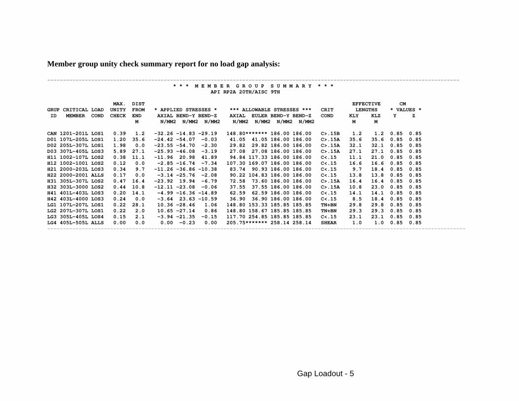
Gap Loadout - 5
Member group unity check summary report for no load gap analysis: ----------------------------------------------------------------------------------------------------------------------------------- * * * M E M B E R G R O U P S U M M A R Y * * * API RP2A 20TH/AISC 9TH MAX. DIST EFFECTIVE CM GRUP CRITICAL LOAD UNITY FROM * APPLIED STRESSES * *** ALLOWABLE STRESSES *** CRIT LENGTHS * VALUES * ID MEMBER COND CHECK END AXIAL BEND-Y BEND-Z AXIAL EULER BEND-Y BEND-Z COND KLY KLZ Y Z M N/MM2 N/MM2 N/MM2 N/MM2 N/MM2 N/MM2 N/MM2 M M CAN 1201-201L LOS1 0.39 1.2 -32.26 -14.83 -29.19 148.80******* 186.00 186.00 C>.15B 1.2 1.2 0.85 0.85 D01 107L-205L LOS1 1.20 35.6 -24.42 -54.07 -0.03 41.05 41.05 186.00 186.00 C>.15A 35.6 35.6 0.85 0.85 D02 205L-307L LOS1 1.98 0.0 -23.55 -54.70 -2.30 29.82 29.82 186.00 186.00 C>.15A 32.1 32.1 0.85 0.85 D03 307L-405L LOS3 5.89 27.1 -25.93 -46.08 -3.19 27.08 27.08 186.00 186.00 C>.15A 27.1 27.1 0.85 0.85 H11 1002-107L LOS2 0.38 11.1 -11.96 20.98 41.89 94.84 117.33 186.00 186.00 C<.15 11.1 21.0 0.85 0.85 H12 1002-1001 LOS2 0.12 0.0 -2.85 -16.74 -7.34 107.30 169.07 186.00 186.00 C<.15 16.6 16.6 0.85 0.85 H21 2000-203L LOS3 0.34 9.7 -11.26 -36.86 -10.38 83.74 90.93 186.00 186.00 C<.15 9.7 18.4 0.85 0.85 H22 2000-2001 ALLS 0.17 0.0 -3.14 -25.76 -2.08 90.22 104.83 186.00 186.00 C<.15 13.8 13.8 0.85 0.85 H31 305L-307L LOS2 0.47 16.4 -23.92 19.94 -6.79 72.58 73.60 186.00 186.00 C>.15A 16.4 16.4 0.85 0.85 H32 303L-3000 LOS2 0.44 10.8 -12.11 -23.08 -0.06 37.55 37.55 186.00 186.00 C>.15A 10.8 23.0 0.85 0.85 H41 401L-403L LOS3 0.20 14.1 -4.99 -16.36 -14.89 62.59 62.59 186.00 186.00 C<.15 14.1 14.1 0.85 0.85 H42 403L-4000 LOS3 0.24 0.0 -3.64 23.63 -10.59 36.90 36.90 186.00 186.00 C<.15 8.5 18.4 0.85 0.85 LG1 107L-207L LOS1 0.22 28.1 10.36 -28.46 1.06 148.80 153.33 185.85 185.85 TN+BN 29.8 29.8 0.85 0.85 LG2 207L-307L LOS1 0.22 2.0 10.65 -27.14 0.86 148.80 158.67 185.85 185.85 TN+BN 29.3 29.3 0.85 0.85 LG3 305L-405L LOS4 0.15 2.1 -3.94 -21.35 -0.15 117.70 254.85 185.85 185.85 C<.15 23.1 23.1 0.85 0.85 LG4 405L-505L ALLS 0.00 0.0 0.00 -0.23 0.00 205.75******* 258.14 258.14 SHEAR 1.0 1.0 0.85 0.85 -------------------------------------------------------------------------------------------------------------------------------------

Structural Modeling Seminar Page - 1
Part 14 - Inertia Loading 1. Tow Inertia Loading Preparation
1) Under “Training Project”, create “Tow” subdirectory 2) Under “Tow” subdirectory, create “Tow Inertia” directory 3) Copy SACINP.DAT model file from “Gap Loadout” directory to “Tow Inertia” directory.
Modifying model for tow inertia load generation
Delete load options LDOPT line, load case selection LCSEL line and all load cases and load combinations. Modifying center of roll CENTER line using coordinate X = -35 m, Y = 0.25 m and Z = -3.5 m
Create tow input file TOWINP.DAT
Tow options need to be set to MN units and center of motion, Coordinate X = -35 m, Y = 0.25 m and Z = -3.5 m Weight group ANOD, LPAD and WKWY are selected using INCWGT line for inertia load generation. Tow input create for 20 degree roll @ 10 seconds period, 10 degree pitch @ 10 seconds period, heave acceleration use 0.2 G. Totally 8 load cases created using MOTION line (or new MOTN line) using “Include effects of Gravity” and “Include Structural Weight” options. +R+H: + Roll + Heave -R+H: - Roll + Heave +R-H: + Roll - Heave -R-H: - Roll - Heave +P+H: + Pitch + Heave -P+H: - Pitch + Heave +P-H: + Pitch - Heave -P-H: - Pitch – Heave The tow input file generated shall looks like following: ------------------------------------------------------------------------------------------------------------- TOWOPT MNEC OR -35.0 0.25 -3.5XYZ INCWGT ANODLPADWKWY MOTION+R+H 12.5 10.0 0.2 G MOTION-R+H-12.5 10.0 0.2 G

Structural Modeling Seminar Page - 2
MOTION+R-H 12.5 10.0 -0.2 G MOTION-R-H-12.5 10.0 -0.2 G MOTION+P+H 10.0 15.0 0.2 G MOTION-P+H -10.0 15.0 0.2 G MOTION+P-H 10.0 15.0 -0.2 G MOTION-P-H -10.0 15.0 -0.2 G *MOTN 1 12.5 10.0 0.2G CEN *MOTN 2 -12.5 10.0 0.2G CEN *MOTN 3 12.5 10.0 -0.2G CEN *MOTN 4 -12.5 10.0 -0.2G CEN *MOTN 5 10.0 15.0 0.2G CEN *MOTN 6 -10.0 15.0 0.2G CEN *MOTN 7 10.0 15.0 -0.2G CEN *MOTN 8 -10.0 15.0 -0.2G CEN END
-------------------------------------------------------------------------------------------------------------
Create tow analysis run file and execute the tow analysis Create run file, run the analysis and browse for results. Compare results generated from MOTION and MOTN.

Structural Modeling Seminar Page - 3
Tow inertia loading summary report: ----------------------------------------------------------------------------------------------------------------------------------- * * * D Y N A M I C L O A D I N G S U M M A T I O N * * * (MOMENTS ABOUT SACS ORIGIN) * JACKET POSITION * ** ANGULAR ACCEL ** *** TRANS ACCEL *** **** FORCE SUMMATION **** ***** MOMENT SUMMATION ***** LOAD ROLL PITCH YAW ROLL PITCH YAW SURGE SWAY HEAVE SURGE SWAY HEAVE ROLL PITCH YAW CASE X Y Z X Y Z X Y Z X Y Z X Y Z ------ (DEG) ------ --- (DEG/SEC**2) --- ------- (G) ------- -------- (KN ) -------- -------- (KN-M ) --------- +R+H 0.0 0.0 0.0 -4.9 0.0 0.0 0.000 0.216 1.176 0.0 -1702.1 -5527.5 29370.4 -245296.3 77044.5 -R+H 0.0 0.0 0.0 4.9 0.0 0.0 0.000 -0.216 1.176 0.0 1702.1 -5502.3 -28757.9 -243875.7 -77044.5 +R-H 0.0 0.0 0.0 -4.9 0.0 0.0 0.000 0.216 0.776 0.0 -1702.1 -3652.1 29266.2 -162124.7 77044.5 -R-H 0.0 0.0 0.0 4.9 0.0 0.0 0.000 -0.216 0.776 0.0 1702.1 -3627.0 -28862.0 -160704.2 -77044.5 +P+H 0.0 0.0 0.0 0.0 -1.8 0.0 -0.174 0.000 1.185 1058.5 0.0 -5417.9 246.7 -215071.3 61.7 -P+H 0.0 0.0 0.0 0.0 1.8 0.0 0.174 0.000 1.185 -1058.5 0.0 -5691.7 370.2 -277640.2 -61.7 +P-H 0.0 0.0 0.0 0.0 -1.8 0.0 -0.174 0.000 0.785 1058.5 0.0 -3542.6 142.5 -131899.7 61.7 -P-H 0.0 0.0 0.0 0.0 1.8 0.0 0.174 0.000 0.785 -1058.5 0.0 -3816.3 266.1 -194468.8 -61.7 -------------------------------------------------------------------------------------------------------------------------------------
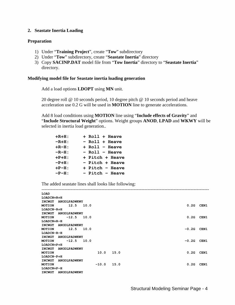
Structural Modeling Seminar Page - 4
2. Seastate Inertia Loading Preparation
1) Under “Training Project”, create “Tow” subdirectory 2) Under “Tow” subdirectory, create “Seastate Inertia” directory 3) Copy SACINP.DAT model file from “Tow Inertia” directory to “Seastate Inertia”
directory.
Modifying model file for Seastate inertia loading generation Add a load options LDOPT using MN unit.
20 degree roll @ 10 seconds period, 10 degree pitch @ 10 seconds period and heave acceleration use 0.2 G will be used in MOTION line to generate accelerations. Add 8 load conditions using MOTION line using “Include effects of Gravity” and “Include Structural Weight” options. Weight groups ANOD, LPAD and WKWY will be selected in inertia load generation.. +R+H: + Roll + Heave -R+H: - Roll + Heave +R-H: + Roll - Heave -R-H: - Roll - Heave +P+H: + Pitch + Heave -P+H: - Pitch + Heave +P-H: + Pitch - Heave -P-H: - Pitch – Heave The added seastate lines shall looks like following: ------------------------------------------------------------------------------------------------------------- LOAD LOADCN+R+H INCWGT ANODLPADWKWY MOTION 12.5 10.0 0.2G CEN1 LOADCN-R+H INCWGT ANODLPADWKWY MOTION -12.5 10.0 0.2G CEN1 LOADCN+R-H INCWGT ANODLPADWKWY MOTION 12.5 10.0 -0.2G CEN1 LOADCN-R-H INCWGT ANODLPADWKWY MOTION -12.5 10.0 -0.2G CEN1 LOADCN+P+H INCWGT ANODLPADWKWY MOTION 10.0 15.0 0.2G CEN1 LOADCN-P+H INCWGT ANODLPADWKWY MOTION -10.0 15.0 0.2G CEN1 LOADCN+P-H INCWGT ANODLPADWKWY
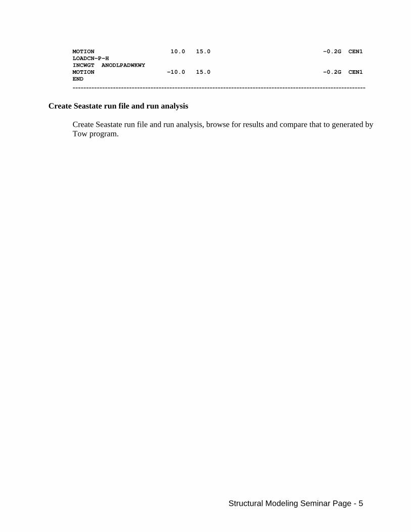
Structural Modeling Seminar Page - 5
MOTION 10.0 15.0 -0.2G CEN1 LOADCN-P-H INCWGT ANODLPADWKWY MOTION -10.0 15.0 -0.2G CEN1 END
-------------------------------------------------------------------------------------------------------------
Create Seastate run file and run analysis Create Seastate run file and run analysis, browse for results and compare that to generated by Tow program.

Structural Modeling Seminar Page - 6
Seastate inertia loading summary report: ----------------------------------------------------------------------------------------------------------------------------------- ****** SEASTATE BASIC LOAD CASE SUMMARY ****** RELATIVE TO MUDLINE ELEVATION LOAD LOAD FX FY FZ MX MY MZ DEAD LOAD BUOYANCY CASE LABEL (KN) (KN) (KN) (KN-M) (KN-M) (KN-M) (KN) (KN) 1 +R+H 0.000 -1702.287 -5528.177 29362.523 -245305.469 77047.141 0.000 0.000 2 -R+H 0.000 1702.287 -5503.011 -28750.020 -243884.656 -77047.141 0.000 0.000 3 +R-H 0.000 -1702.287 -3652.597 29258.354 -162130.672 77047.141 0.000 0.000 4 -R-H 0.000 1702.287 -3627.434 -28854.174 -160710.062 -77047.141 0.000 0.000 5 +P+H 1058.641 0.000 -5418.664 246.689 -215084.109 61.657 0.000 0.000 6 -P+H -1058.641 0.000 -5692.363 370.243 -277645.719 -61.656 0.000 0.000 7 +P-H 1058.641 0.000 -3543.078 142.549 -131909.766 61.657 0.000 0.000 8 -P-H -1058.641 0.000 -3816.773 266.102 -194470.703 -61.656 0.000 0.000 -------------------------------------------------------------------------------------------------------------------------------------

Tow Fatigue - 1
Part 15 - Tow Fatigue Preparation
1) Under “Training Project”, create “Tow” subdirectory 2) Under “Tow” subdirectory, create “Tow Fatigue” directory 3) Copy SACINP.DAT model file from “Tow Inertia” directory to “Tow Fatigue” directory.
Modifying Model file to include Response Amplitude Operator values
Delete the CENTER line from model. Eight (8) direction RAOs will be input at center of motion X = -35.00 m, Y = 0.25 m and Z = -3.50 m. There RAOs are corresponding to direction 000, 045, 090, 135, 180, 225, 270 and 315. Part of the added RAO lines shall looks like following: ------------------------------------------------------------------------------------------------------------- RAO HEAD -35.0000 0.2500 -3.5000R000 DP RAO DP40.000 0.798-90.5 0.008-1.60 0.3206.420 0.0130.020 0.367-84.6 0.03398.70 RAO DP39.000 0.796-90.4 0.006-2.40 0.3186.580 0.013-1.07 0.348-85.4 0.03397.80 … RAO DP 6.000 0.025-68.1 -70.0 -56.1 -71.5 0.016-65.9 0.003113.0 RAO DP 5.000 0.007-7.08 -7.90 175.0 -9.95 0.007-6.25 173.0 RAO HEAD 45.000 -35.0000 0.2500 -3.5000R045 DP RAO DP40.000 0.564-90.5 0.574-89.0 0.3206.860 0.24391.70 0.262-84.2 0.020102.0 RAO DP39.000 0.564-90.4 0.572-89.0 0.3187.020 0.23091.30 0.243-85.0 0.020100.0 … RAO DP 6.000 0.018-68.1 0.018-68.0 -50.4 0.013114.0 0.013-65.8 112.0 RAO DP 5.000 0.004-7.08 0.004-7.00 -0.70 174.0 -6.22 173.0 RAO HEAD 90.000 -35.0000 0.2500 -3.5000R090 DP RAO DP40.000 63.10 0.812-89.0 0.3206.580 0.34191.90 129.0 -110. RAO DP39.000 65.50 0.810-89.0 0.3186.730 0.32291.40 137.0 -110. … RAO DP 6.000 -74.4 0.024-68.0 -51.1 0.013114.0 -69.4 106.0 RAO DP 5.000 -12.2 0.006-7.00 -1.03 174.0 -11.7 168.0 RAO HEAD135.000 -35.0000 0.2500 -3.5000R135 DP RAO DP40.000 0.56489.50 0.574-89.0 0.3207.100 0.24391.70 0.26295.90 0.026-84.9 RAO DP39.000 0.56489.60 0.572-89.0 0.3187.260 0.23091.20 0.24395.10 0.026-85.3 … RAO DP 6.000 0.018112.0 0.018-68.0 -50.3 0.013114.0 0.013114.0 -67.0 RAO DP 5.000 0.004173.0 0.004-7.00 -0.57 174.0 174.0 -6.37 RAO HEAD180.000 -35.0000 0.2500 -3.5000R180 DP RAO DP40.000 0.79889.50 0.008-1.30 0.3206.580 0.0130.140 0.36795.40 0.026-82.3 RAO DP39.000 0.79889.60 0.006-2.10 0.3186.740 0.013-0.94 0.34894.70 0.033-83.1 … RAO DP 6.000 0.024112.0 108.0 -56.3 109.0 0.013114.0 -67.4 RAO DP 5.000 0.006173.0 170.0 175.0 169.0 174.0 -6.58 RAO HEAD225.000 -35.0000 0.2500 -3.5000R225 DP RAO DP40.000 0.56489.40 0.57488.90 0.3226.990 0.243-81.2 0.26296.30 0.020-79.3 RAO DP39.000 0.56489.50 0.57289.00 0.3187.170 0.230-82.0 0.24395.50 0.020-80.6 … RAO DP 6.000 0.018112.0 0.018112.0 130.0 0.013-65.9 0.013114.0 -67.7 RAO DP 5.000 0.004173.0 0.004173.0 179.0 -6.25 174.0 -6.74 RAO HEAD270.000 -35.0000 0.2500 -3.5000R270 DP

Tow Fatigue - 2
RAO DP40.000 -99.3 0.81289.10 0.3206.320 0.341-82.6 -82.4 79.40 RAO DP39.000 -102. 0.81089.20 0.3186.490 0.322-83.3 -46.5 79.30 … RAO DP 6.000 106.0 0.024112.0 130.0 0.013-65.9 111.0 -74.2 RAO DP 5.000 168.0 0.006173.0 179.0 -6.27 167.0 -11.5 RAO HEAD315.000 -35.0000 0.2500 -3.5000R315 DP RAO DP40.000 0.564-90.6 0.57488.90 0.3206.810 0.243-81.2 0.262-83.8 0.02696.90 RAO DP39.000 0.564-90.5 0.57289.00 0.3186.980 0.230-82.0 0.243-84.6 0.02696.40 … RAO DP 6.000 0.018-68.1 0.018112.0 130.0 0.013-65.9 0.013-65.8 113.0 RAO DP 5.000 0.004-7.08 0.004173.0 179.0 -6.25 -6.23 174.0
-------------------------------------------------------------------------------------------------------------
Create Tow input file TOWINP.TOWFTG to generate and solve tow inertia loads, Tow options line to define MN unit will be used; An INCRAO line is added to use RAOs from model file. A weight selection INCWGT line will be used to include weight group ANOD, LPAD and WKWY for inertia load generation. Inertia loads will be created using WAVDEF line for unit wave heights in wave period for 25.0, 18.0, 11.0, 10.0, 9.0 and 5.0 seconds for 8 wave directions, that is 000, 045, 090, 135, 180, 225, 270 and 315. Number of load conditions per wave will be four (4). Load case numbers can be left blank or shall be carefully counted for avoid problems. The tow input file generated for tow fatigue shall looks like following: ------------------------------------------------------------------------------------------------------------- TOW INPUT FOR JACKET TOW FATIGUE ANALYSIS TOWOPT MNEC WPOR XYZ INCRAO INCWGT ANODLPADWKWY WAVDEF 1 4 1.00 25.0 0.0 WAVDEF 5 4 1.00 18.0 0.0 WAVDEF 9 4 1.00 11.0 0.0 WAVDEF 13 4 1.00 10.0 0.0 WAVDEF 17 4 1.00 9.00 0.0 WAVDEF 21 4 1.00 5.00 0.0 WAVDEF 25 4 1.00 25.0 45.0 WAVDEF 29 4 1.00 18.0 45.0 WAVDEF 33 4 1.00 11.0 45.0 WAVDEF 37 4 1.00 10.0 45.0 WAVDEF 41 4 1.00 9.00 45.0 WAVDEF 45 4 1.00 5.00 45.0 WAVDEF 49 4 1.00 25.0 90.0 WAVDEF 53 4 1.00 18.0 90.0 WAVDEF 57 4 1.00 11.0 90.0 WAVDEF 61 4 1.00 10.0 90.0 WAVDEF 65 4 1.00 9.00 90.0 WAVDEF 69 4 1.00 5.00 90.0 WAVDEF 73 4 1.00 25.0 135.0 WAVDEF 77 4 1.00 18.0 135.0 WAVDEF 81 4 1.00 11.0 135.0 WAVDEF 85 4 1.00 10.0 135.0 WAVDEF 89 4 1.00 9.00 135.0 WAVDEF 93 4 1.00 5.00 135.0
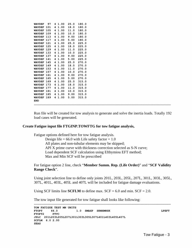
Tow Fatigue - 3
WAVDEF 97 4 1.00 25.0 180.0 WAVDEF 101 4 1.00 18.0 180.0 WAVDEF 105 4 1.00 11.0 180.0 WAVDEF 109 4 1.00 10.0 180.0 WAVDEF 113 4 1.00 9.00 180.0 WAVDEF 117 4 1.00 5.00 180.0 WAVDEF 121 4 1.00 25.0 225.0 WAVDEF 125 4 1.00 18.0 225.0 WAVDEF 129 4 1.00 11.0 225.0 WAVDEF 133 4 1.00 10.0 225.0 WAVDEF 137 4 1.00 9.00 225.0 WAVDEF 141 4 1.00 5.00 225.0 WAVDEF 145 4 1.00 25.0 270.0 WAVDEF 149 4 1.00 18.0 270.0 WAVDEF 153 4 1.00 11.0 270.0 WAVDEF 157 4 1.00 10.0 270.0 WAVDEF 161 4 1.00 9.00 270.0 WAVDEF 165 4 1.00 5.00 270.0 WAVDEF 169 4 1.00 25.0 315.0 WAVDEF 173 4 1.00 18.0 315.0 WAVDEF 177 4 1.00 11.0 315.0 WAVDEF 181 4 1.00 10.0 315.0 WAVDEF 185 4 1.00 9.00 315.0 WAVDEF 189 4 1.00 5.00 315.0 END
------------------------------------------------------------------------------------------------------------- Run file will be created for tow analysis to generate and solve the inertia loads. Totally 192 load cases will be generated.
Create Fatigue input file FTGINP.TOWFTG for tow fatigue analysis,
Fatigue options defined here for tow fatigue analysis. Design life = 66.0 with Life safety factor = 1.0 All plates and non-tubular elements may be skipped; API X prime curve with thickness correction selected as S-N curve;
Load dependent SCF calculation using Efthymiou EFT method; Max and Min SCF will be prescribed
For fatigue option 2 line, check “Member Summ. Rep. (Life Order)” and “SCF Validity Range Check”.
Using joint selection line to define only joints 201L, 203L, 205L, 207L, 301L, 303L, 305L, 307L, 401L, 403L, 405L and 407L will be included for fatigue damage evaluations. Using SCF limits line SCFLM to define max. SCF = 6.0 and min. SCF = 2.0. The tow input file generated for tow fatigue shall looks like following: ------------------------------------------------------------------------------------------------------------- TOW FATIGUE TEST MN UNITS FTOPT 66.0 1.0 SMAXP SKMXMNSK LPEFT FTOPT2 PTVC JSLC 201L203L205L207L301L303L305L307L401L403L405L407L SCFLM 6.0 2.00 SEAS

Tow Fatigue - 4
* (SACS DIR - DIRECTIONAL SECTOR) * 0 DEGREES - FROM NORTHWEST FTLOAD 1 0.01 1.0 SPC WSPEC 1 PM 7.50 12.500 .00013 WSPEC 1 PM 7.00 11.500 .00025 … WSPEC 1 PM 0.50 4.500 .31507 WSPEC 1 PM 0.50 6.500 .11644 * 45 DEGREES - FROM WEST SECTOR FTLOAD 2 0.01 1.0 SPC WSPEC 2 PM 7.50 10.500 .00013 WSPEC 2 PM 6.50 11.500 .00013 … WSPEC 2 PM 0.50 5.500 .00685 WSPEC 2 PM 0.50 6.500 .10274 * 90 DEGREES - FROM SOUTHWEST SECTOR FTLOAD 3 0.01 1.0 SPC WSPEC 3 PM 7.00 9.500 .00025 WSPEC 3 PM 6.50 9.500 .00013 … WSPEC 3 PM 0.50 4.500 .32192 WSPEC 3 PM 0.50 6.500 .10959 * 135 DEGREES - FROM SOUTH SECTOR FTLOAD 4 0.01 1.0 SPC WSPEC 4 PM 11.00 12.500 .00013 WSPEC 4 PM 10.50 11.500 .00025 … WSPEC 4 PM 0.50 5.500 .02740 WSPEC 4 PM 0.50 6.500 .15068 * 180 DEGREES - FROM SOUTHEAST SECTOR FTLOAD 5 0.01 1.0 SPC WSPEC 5 PM 11.50 12.500 .00050 WSPEC 5 PM 11.00 12.500 .00038 … WSPEC 5 PM 0.50 6.500 .19178 WSPEC 5 PM 0.50 8.500 .00685 * 225 DEGREES - FROM EAST SECTOR FTLOAD 6 0.01 1.0 SPC WSPEC 6 PM 12.00 13.500 .00025 WSPEC 6 PM 11.00 12.500 .00013 … WSPEC 6 PM 0.50 5.500 .02740 WSPEC 6 PM 0.50 6.500 .11644 * 270 DEGREES - FROM NORTHEAST SECTOR FTLOAD 7 0.01 1.0 SPC WSPEC 7 PM 11.00 13.500 .00013 WSPEC 7 PM 10.50 13.500 .00025 … WSPEC 7 PM 0.50 5.500 .03425 WSPEC 7 PM 0.50 6.500 .10274 * 315 DEGREES - FROM NORTH SECTOR FTLOAD 8 0.01 1.0 SPC WSPEC 8 PM 9.00 13.500 .00013 WSPEC 8 PM 8.50 13.500 .00013 … WSPEC 8 PM 0.50 4.500 .27397 WSPEC 8 PM 0.50 6.500 .09589 EXTRAC HEAD AE.50 END
-------------------------------------------------------------------------------------------------------------

Tow Fatigue - 5
Create fatigue run file and run analysis, browse for results.

Tow Fatigue - 6
Portion of tow fatigue analysis report for joint 407L and 403L: ----------------------------------------------------------------------------------------------------------------------------------- * * * M E M B E R F A T I G U E R E P O R T * * * (DAMAGE ORDER) ORIGINAL CHORD REQUIRED JOINT MEMBER GRUP TYPE OD WT JNT MEM LEN. GAP * STRESS CONC. FACTORS * FATIGUE RESULTS OD WT ID ID (CM) (CM) TYP TYP (M ) (CM) AX-CR AX-SD IN-PL OU-PL DAMAGE LOC SVC LIFE (CM) (CM) 407L 403L-407L H41 TUB 32.38 1.250 Y BRC 12.12 0.00 3.00 6.00 2.35 3.53 .23587-7 L 27981.+5 407L 407L-507L LG4 TUB 107.00 3.500 Y CHD 12.12 2.53 4.74 2.00 2.74 .0000000 T INFINITE 407L 405L-407L H41 TUB 32.38 1.250 Y BRC 12.12 0.00 3.00 6.00 2.35 3.53 .32978-4 R 2001334. 407L 407L-507L LG4 TUB 107.00 3.500 Y CHD 12.12 2.53 4.74 2.00 2.74 .35694-5 R 18491.+3 407L 407L-4000 H42 TUB 32.38 1.250 Y BRC 12.12 0.00 3.00 6.00 2.35 3.51 .31723-5 R 20805.+3 407L 407L-507L LG4 TUB 107.00 3.500 Y CHD 12.12 2.53 4.71 2.00 2.72 .19701-6 R 33501.+4 ---------------------------------------------------------------------------------------------------------------------------------- 403L 307L-403L D03 TUB 40.75 1.500 K BRC 12.12 30.96 2.70 2.63 2.78 2.14 .0000000 T INFINITE 403L 303L-403L LG3 TUB 107.00 3.500 K CHD 12.12 2.69 2.75 2.00 2.03 .0000000 T INFINITE 403L 401L-403L H41 TUB 32.38 1.250 Y BRC 12.12 0.00 3.00 6.00 2.35 3.53 .32891-4 L 2006652. 403L 403L-503L LG4 TUB 107.00 3.500 Y CHD 12.12 2.53 4.74 2.00 2.74 .35799-5 L 18436.+3 403L 403L-407L H41 TUB 32.38 1.250 K BRC 12.12 30.96 4.06 5.14 2.35 3.57 .37433-8 L 17631.+6 403L 403L-503L LG4 TUB 107.00 3.500 K CHD 12.12 3.44 4.23 2.00 2.77 .0000000 T INFINITE 403L 403L-4000 H42 TUB 32.38 1.250 Y BRC 12.12 0.00 3.00 6.00 2.35 3.51 .51932-5 L 12709.+3 403L 403L-503L LG4 TUB 107.00 3.500 Y CHD 12.12 2.53 4.71 2.00 2.72 .36860-6 L 17906.+4 -------------------------------------------------------------------------------------------------------------------------------------

Launch and Post Launch - 1
Part 16 - Launch and Post Launch Preparation
1) Under “Training Project”, create “Launch” subdirectory 2) Copy SACINP.DAT model file from “\Tow\Tow Inertia” directory to “Launch”
directory. Create Launch input file LNHINP.DAT for jacket launch analysis
For Launch options, use MN unit for both input and output; Set “Accel Velocity Disp Plot Type” as NPF for neutral picture file. Input water depth 79.50 m and seawater density as 1.025 MT/m^3. A launch time control TIME line is need. Set stop time to 625.0 seconds, set output time intervals to 10.0, 5.0, 1.0, 1.0 and 5.0 corresponding to phase 1 to 5. Minimum launch time step = 1.0E-8 second and error control parameter =1.0. Jacket Orientation JACKET line will be added to define jacket position relative to barge. Joint 401L, 405L and 101L will be input as 1st, 2nd and 3rd joints. Distance from barge front to 1st joint = 84.0 m; Length of Launch Framing = 82.0 m; Density of construction material and added load = 7.85 MT/m^3 Barge description will be input on BARGE1 line: Height of barge = 7.50 m; Width of barge = 18.50 m; Bottom Length of barge = 75.0 m; Forward Extension = 5.0 m; Aft Extension =7.50 m; Forward initial draft = 2.25 m; Aft initial draft = 4.50 m; Number of side and bottom increments = 20 Additional Barge description will be input on BARGE2 line: Skid height = 1.50 m; Rocker Pin Location = 84.0 m; Rocker arm depth = 2.75 m; Winch speed = 0.1 m/sec; Both drag and added mass coefficients = 1.0 Weight groups ANOD, LPAD and WKWY will be selected using INCWGT line. Friction coefficients will be input using FRICT line to define: Static friction coefficient = 0.1 Dynamic friction coefficient = 0.05 for speed from 0.0 t 10.0 m/sec

Launch and Post Launch - 2
Member group CAN will be deleted from launch analysis using GRPDEL line. A geometry plot PLTGM line added to select “Plot Type” = Full and using STEP for plot intervals. Initial jacket on barge will be plotted. The launch input file generated shall looks like following: ------------------------------------------------------------------------------------------------------------- LAUNCH EXAMPLE LAUNCH MNMN PT PF 79.50 1.025 TIME 625.00 10.0 5.0 1.0 1.0 5.0 1.0E-8 1.0 JACKET 401L405L101L 84.0 82.0+Z 7.85 7.85 BARGE BARGE1 7.50 18.50 75.00 5.0 7.50 2.25 4.50 20.0 20.0 BARGE2 1.50 84.0 2.75 0.10 1.0 1.0 INCWGT ANODLPADWKWY FRICT FRICT 0.1 0.00 0.05 10.00 0.05 GRPDEL CAN PLTGM FLJB 1 END
-------------------------------------------------------------------------------------------------------------
Create Launch run file and run the analysis Create launch run file and run the launch analysis, browse for results.
Create Post Launch input file PLNINP.DAT for jacket post launch analysis Copy launch input file LNHINP.DAT to post launch input file PLNINP.DAT. Rename launch options header from LAUNCH to PSTLNH; Remove time control TIME line and geometry plot PLTGM line. Add launch load definition LLODA line to select various kinds of points for load case generation. Two time points 100 seconds and 475 seconds will be selected to create load case L100 and L475. The post launch input file generated shall looks like following: ------------------------------------------------------------------------------------------------------------- LAUNCH EXAMPLE PSTLNH MNMN PT -79.50 1.025 JACKET 401L405L101L 84.0 82.0+Z 7.85 7.85 BARGE BARGE1 7.50 18.50 75.00 5.0 7.50 2.25 4.50 20.0 20.0 BARGE2 1.50 84.0 2.75 0.10 1.0 1.0 INCWGT ANODLPADWKWY FRICT

Launch and Post Launch - 3
FRICT 0.1 0.00 0.05 10.00 0.05 GRPDEL CAN LLODA LLODA L100TME 100.0L475TME 475.0 END
------------------------------------------------------------------------------------------------------------- Create post launch run file, run the analysis and browse for results.
Flotation and Upending - 1
Part 17 - Flotation and Upending
Preparation
1) Under “Training Project”, create “Flotation” subdirectory 2) Copy SACINP.DAT model file from “Launch” directory to “Flotation” directory.
Modifying model for flotation analysis
Launch model can be directly used for flotation analysis without modification.
Creating flotation input FLTINP.DAT for flotation analysis Flotation options:
MN units will be selected for both input and output; Water depth = 79.50 m with water weight density = 1.025 MT/m^3; Maximum number of iterations = 500 with weight iteration tolerance = 0.001 and moment iteration tolerance = 0.01; Upending type = SHJF for single hook with jacket initially floating.
A jacket orientation line JCKO is required for locate the initial position of jacket: Material weight density = 7.849 MT/m^3 with 1.0 weight contingency factor;
Joint 103L, 107L and 503L will be input to Jacket Orientation joint #1 to #3 to determine jacket initial flotation position; Added load density = 7.849 MT/m^3.
Plot neutral picture file parameters PLOTH line needed for plotting, Plot destination = FILE only; All steps will be plotted for pitch views; A summary report line PLTRQ needed to request various kinds of reports, Hook loads, Sling loads and Mudline clearances will be reported.
Member group CAN will be deleted from flotation analysis using GRPDEL line. Weight groups ANOD, LPAD and WKWY will be selected using INCWGT line. Leg definition line LEGDEF will be used to define 101L-501L as LEG1, 103L-503L as LEG3, 105L-505L as LEG5, and 07L-507L as LEG7. Crane hook definition line HOOK added to define hook label as MAIN; Four SLING lines added to define attach joints and parameters of lifting slings, SLING1 will be attached to joint 401L with sling length =21.50 m; SLING3 will be attached to joint 403L with sling length =20.00 m;

Flotation and Upending - 2
SLING5 will be attached to joint 405L with sling length =21.50 m; SLING7 will be attached to joint 407L with sling length =20.00 m; Sling diameter = 10 cm and elastic modulus = 7 MN/cm^2; Sling weight for 21.5 m sling = 1.6 MT and 1.5 MT for 20 m. A BEGIN line needed to signal program starting the flotation sequence analysis; Step 1: Hook elevation to 3.5 m in 2 increment using hook elevation HOOKEL line; Step 2: Hook elevation to 4.50 in 2 increments using hook elevation HOOKEL line; Step 3: Hook elevation to 7.50 in 5 increments using hook elevation HOOKEL line; Step 4: Hook elevation to 11.00 in 5 increments using hook elevation HOOKEL line; Step 5: Hook elevation to 13.75 in 5 increments using hook elevation HOOKEL line; Step 6: Hook elevation to 17.00 in 5 increments using hook elevation HOOKEL line; Step 7: Hook elevation to 25.00 in 15 increments using hook elevation HOOKEL line; Step 8: LEG1 and LEG5 will be flooded in 20 increments using flood element definition line FLLEG; Step 9: LEG3 and LEG7 will be flooded in 20 increments using flood element definition line FLLEG; Step 10: Hook elevation to 22.00 in 4 increments using hook elevation HOOKEL line; The flotation input file generated shall looks like following: ------------------------------------------------------------------------------------------------------------- FLOTATION ANALYSIS EXAMPLE FLTOPT MN 79.50 1.025 500 SHJF 0.001 0.05 JCKO +Z 7.849103L107L503L 1.0 7.849 PLOTH ALPV MT 27.9421.59.2159 PLTRQ HL MC SL GRPDEL CAN INCWGT ANODLPADWKWY LEGDEF 101L501LLEG1 103L503LLEG3 105L505LLEG5 107L507LLEG7 HOOK MAIN 0.0 SLING J401L 21.5 10.0 7.00 SLING1 1.60 SLING J403L 20.0 10.0 7.00 SLING3 1.50 SLING J405L 21.5 10.0 7.00 SLING5 1.60 SLING J407L 20.0 10.0 7.00 SLING7 1.50 BEGIN STEP 2 HOOKEL MAIN 3.50 STEP 2 HOOKEL MAIN 4.50 STEP 5 HOOKEL MAIN 7.50 STEP 5 HOOKEL MAIN 11.00 STEP 5 HOOKEL MAIN 13.75 STEP 5 HOOKEL MAIN 17.00 STEP 15 HOOKEL MAIN 25.00 STEP 20 FLLEG 1.0LEG1 LEG5 STEP 20 FLLEG 1.0LEG3 LEG7 STEP 4

Flotation and Upending - 3
HOOKEL MAIN 22.00 END
-------------------------------------------------------------------------------------------------------------
Creating flotation run file and run the analysis Create flotation run file and run the analysis. Browse for results.

1
Tutorial Problem 1. Model description: The frame is 10’ x 20’, the upright columns are 10” x 10” x ¼” box sections and the horizontal beam is an AISC W18x40 wide flange. Three load cases will be considered, Load case 1 is a uniform dead load of -1.0 kips/ft along the horizontal beam; Load case 2 is a 16 kips concentrated wind load; Load case 3 is a load combination of load case 1 and 2, each at 100% and factored at 133%. 2. Create Project and major task “Structural Modeling”: Launch SACS Executive; Under Project/Task menu select Add project Type in Name “Tutorial” Type in Location “C:\...\Tutorial” Type in Description “Demonstration Problem” Type in Worksheet file “Tutorial” then click OK Accept and create the new directory (Refer to following “Add New Project” figure)
Under Project/Task menu select Add major task Type in Name Structural Modeling Type in description Create Model File Type in File Identifier dat Then click OK (Refer to following “Add New Task” figure)
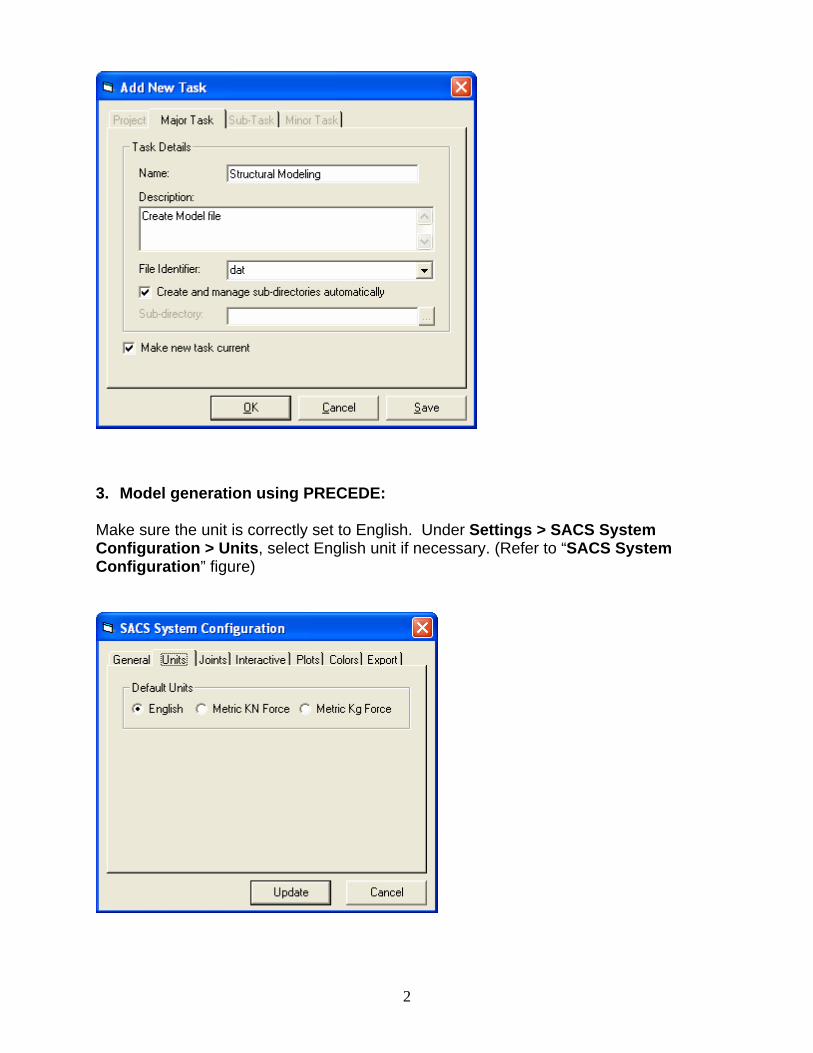
2
3. Model generation using PRECEDE: Make sure the unit is correctly set to English. Under Settings > SACS System Configuration > Units, select English unit if necessary. (Refer to “SACS System Configuration” figure)

3
a) Launch PRECEDE
Click Modeling > Precede Select “Created new model” then OK (Refer to “PRECEDE” Figure)
For new structure select “None”; Type in Title “Tutorial Frame” Deselect “Use alphanumeric jacket joint names with tags” Then click OK (Refer to “New Structure” Figure) PRECEDE program will be launched (Refer to “PrecedePro” figure)
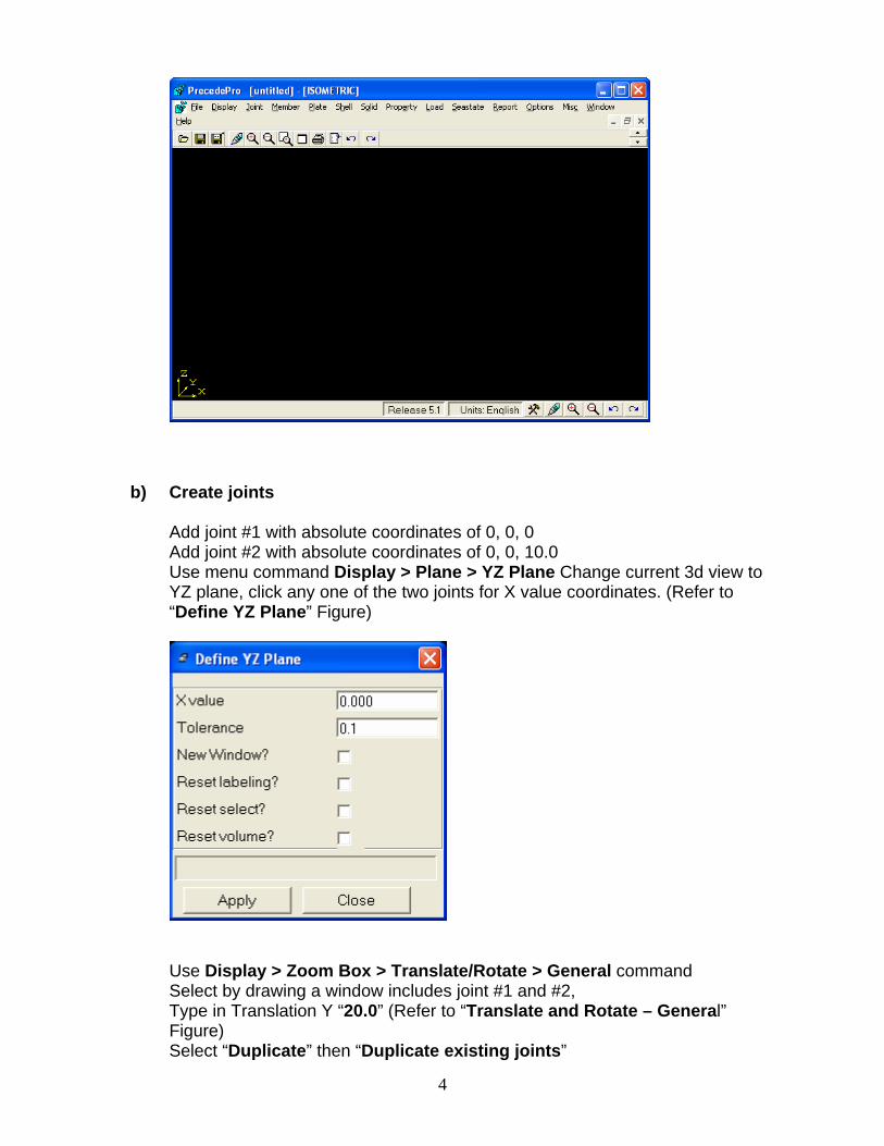
4
b) Create joints
Add joint #1 with absolute coordinates of 0, 0, 0 Add joint #2 with absolute coordinates of 0, 0, 10.0 Use menu command Display > Plane > YZ Plane Change current 3d view to YZ plane, click any one of the two joints for X value coordinates. (Refer to “Define YZ Plane” Figure)
Use Display > Zoom Box > Translate/Rotate > General command Select by drawing a window includes joint #1 and #2, Type in Translation Y “20.0” (Refer to “Translate and Rotate – General” Figure) Select “Duplicate” then “Duplicate existing joints”

5
Type in Number of duplications “1” (Refer to “Translate and Rotate – Duplicate” Figure) Click OK and created joints #3 and #4
Use Display > Labeling > Joint to display joint names. We have created four corner joints of the frame. (Refer to “PrecedePro [untitled]” Figure)
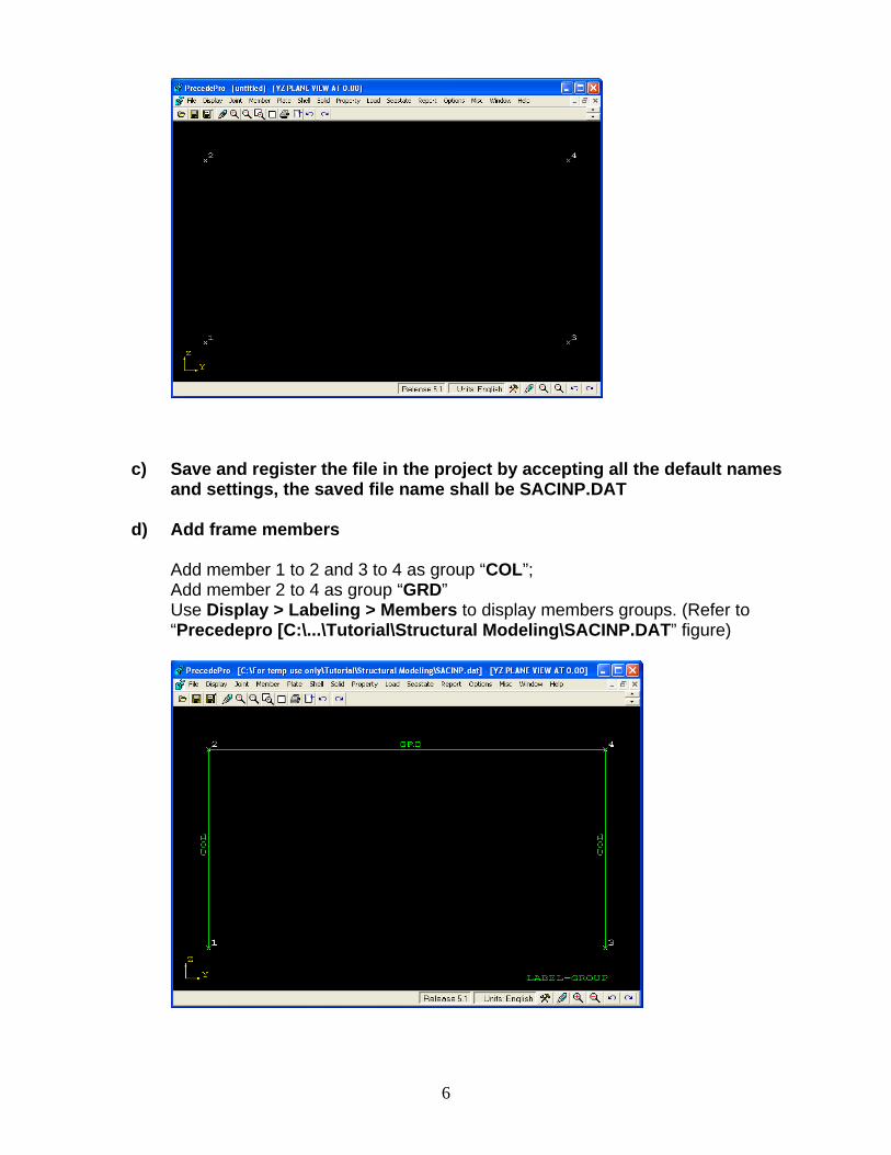
6
c) Save and register the file in the project by accepting all the default names and settings, the saved file name shall be SACINP.DAT
d) Add frame members
Add member 1 to 2 and 3 to 4 as group “COL”; Add member 2 to 4 as group “GRD” Use Display > Labeling > Members to display members groups. (Refer to “Precedepro [C:\...\Tutorial\Structural Modeling\SACINP.DAT” figure)

7
e) Define member properties
Select Property > Member Group and Choose “COL” then “Define” Select Group type as “General” Type in Section label “Box10” (Refer to “Define Member Group COL” Figure)
Choose “GRD” then “Define” Select Group type as “General” Browse in section label to find “W18X40” (Refer to “Define Member Group GRD” Figure)

8
Select “Close” to quit member group definition window
f) Define member sections
Select Property > Member Section Choose “Box10” Select Section Type as “Box” Then “Define” (Refer to “Member Section” Figure)
Type in Side depth “10.0” Type in Side wall thickness “0.25” Type in Width “10.0” Type in Top wall Thickness “0.25” (Refer to “Define Section BOX10” Figure)
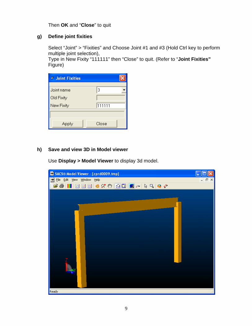
9
Then OK and “Close” to quit
g) Define joint fixities
Select “Joint” > “Fixities” and Choose Joint #1 and #3 (Hold Ctrl key to perform multiple joint selection), Type in New Fixity “111111” then “Close” to quit. (Refer to “Joint Fixities” Figure)
h) Save and view 3D in Model viewer
Use Display > Model Viewer to display 3d model.

10
i) Add load case #1
Select Load > Members then Choose member 2-4 and click “Apply” Type in Load Condition “1” Type in Load ID “Dead” Select Load type as “Distributed” then Click “Add” (Refer to “Member Loads” Figure)
Type in Initial load value “-1.0” Type in final load value “-1.0” then click OK (Refer to “Member Distributed” Figure)
Review the force summary report and Click “Save”, the load will display in the graphics window also. (Refer to “Sum of Forces Report” Figure)

11
j) Add load case #2
Select Load > Joints then Choose joint #2 and click “Apply” Type in Load Condition “2” Type in Load ID “WIND” then “Add” (Refer to “Joint Loads” Figure)
Type in Fy “16.0” then OK (Refer to “Joint Loads LC2” Figure)
Review force summary report and “Save”, note the force also shown in the graphics window. (Refer to “Sum of Forces Report” Figure)
k) Add load case #3

12
Select Load > Combine Load Conditions Type in LC combination label “3” then “Define” Choose Load case 1 and 2 then “OK” and “Close” to quit (Refer to “LC Combination Data for LC 3” Figure)
l) Save
m) Define allowable stress modifier
Select Options > Allowable Stress/Mat Factor Choose load case 3 and type in factor as “1.333” then “Update” to quit (Refer to “Allowable Stress/Material Factor” Figure)
Save, Exit PRECEDE program.
4. Use Datagen to make modifications to model file SACINP.DAT:
Choose Modeling > DataGen, select Edit existing data file and select SACINP.DAT. Change options line: Double click the OPTIONS line, make necessary changes as

13
- General Window: select APUC for code check option – Tubular API 21st
edition and others AISC 9th edition; (Refer to “SACS Options – General” Figure)
- Report Window: Choose appropriate print options as desired (Refer to “SACS
Options – Report” Figure)

14
Double Click AMOD line and Change allowable stress modifier from 1.333 to 1.33 (Refer to “Allowable Stress Modifier” Figure)
Save file and exit from DataGen program, the model file now is ready to run.
5. Create Major Task “Static Analysis”:
Use Project/Task > Add major task again Type in Name “Static Analysis” Type in description “Run Static Analysis” Type in File Identifier “sta” Then click OK (Refer to “Add New Task” Figure)
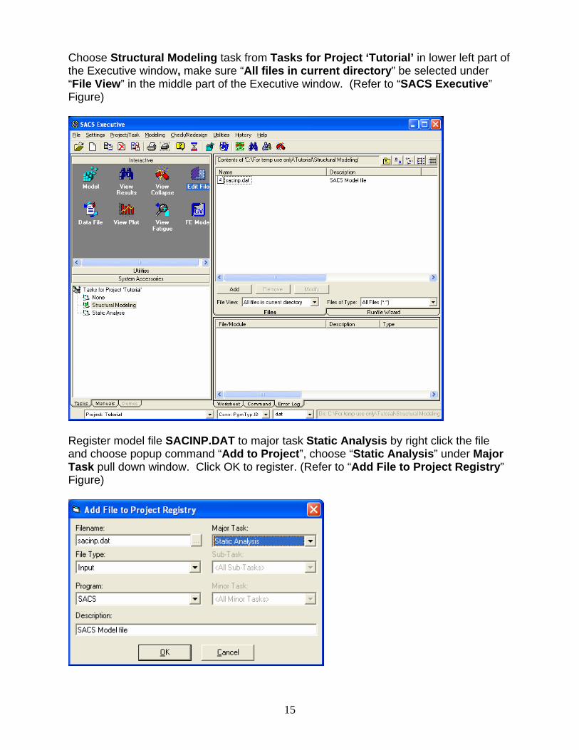
15
Choose Structural Modeling task from Tasks for Project ‘Tutorial’ in lower left part of the Executive window, make sure “All files in current directory” be selected under “File View” in the middle part of the Executive window. (Refer to “SACS Executive” Figure)
Register model file SACINP.DAT to major task Static Analysis by right click the file and choose popup command “Add to Project”, choose “Static Analysis” under Major Task pull down window. Click OK to register. (Refer to “Add File to Project Registry” Figure)
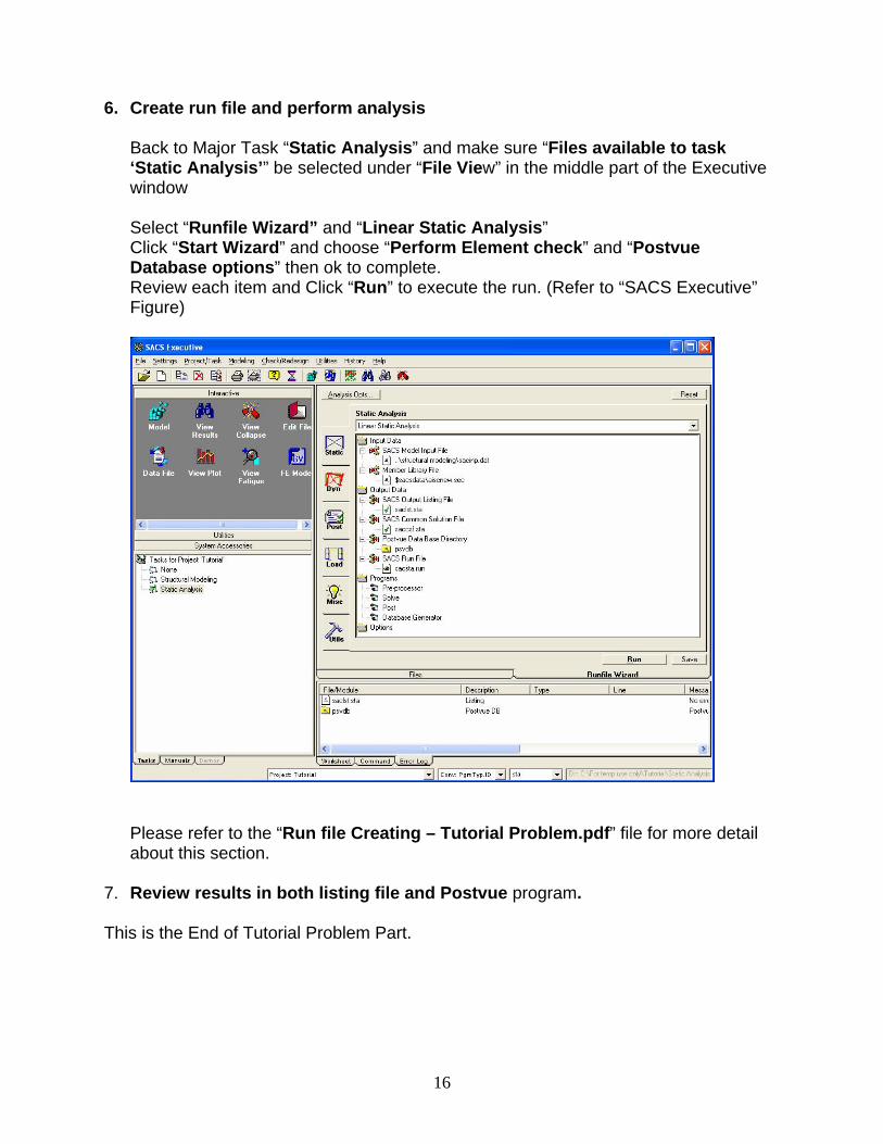
16
6. Create run file and perform analysis
Back to Major Task “Static Analysis” and make sure “Files available to task ‘Static Analysis’” be selected under “File View” in the middle part of the Executive window Select “Runfile Wizard” and “Linear Static Analysis” Click “Start Wizard” and choose “Perform Element check” and “Postvue Database options” then ok to complete. Review each item and Click “Run” to execute the run. (Refer to “SACS Executive” Figure)
Please refer to the “Run file Creating – Tutorial Problem.pdf” file for more detail about this section.
7. Review results in both listing file and Postvue program. This is the End of Tutorial Problem Part.

17
Appendix – SACS input file data deck for SACINP.DAT 12345678901234567890123456789012345678901234567890123456789012345678901245678 Tutorial Frame OPTIONS EN SDUC 2 1 C PTPT PTPT AMOD AMOD 3 1.33 SECT SECT BOX10 BOX 10.000.250 10.000.250 GRUP GRUP COL BOX10 29.0011.6036.00 1 1.001.00 N490.00 GRUP GRD W18X40 29.0011.6036.00 1 1.001.00 N490.00 MEMBER MEMBER 1 2 COL MEMBER 3 4 COL MEMBER 2 4 GRD JOINT JOINT 1 0. 0. 0. 111111 JOINT 2 0. 0. 10. JOINT 3 0. 20. 0. 111111 JOINT 4 0. 20. 10. LOAD LOADCN 1 LOAD Z 2 4 -1.0000 -1.0000 GLOB UNIF DEAD LOADCN 2 LOAD 2 16.0000 GLOB JOIN WIND LCOMB LCOMB 3 1 1.000 2 1.000 END ***SPMB** 1 2 1 2 3 4 3 4 2 4 2 4 END 12345678901234567890123456789012345678901234567890123456789012345678901245678