ja indu in mao review
TRANSCRIPT

7/27/2019 Ja Indu in Mao Review
http://slidepdf.com/reader/full/ja-indu-in-mao-review 1/34
Statistical Pattern Recognition: A ReviewAnil K. Jain, Fellow , IEEE , Robert P.W. Duin, and Jianchang Mao, Senior Member , IEEE
AbstractÐThe primary goal of pattern recognition is supervised or unsupervised classification. Among the various frameworks in
which pattern recognition has been traditionally formulated, the statistical approach has been most intensively studied and used inpractice. More recently, neural network techniques and methods imported from statistical learning theory have been receiving
increasing attention. The design of a recognition system requires careful attention to the following issues: definition of pattern classes,
sensing environment, pattern representation, feature extraction and selection, cluster analysis, classifier design and learning, selection
of training and test samples, and performance evaluation. In spite of almost 50 years of research and development in this field, the
general problem of recognizing complex patterns with arbitrary orientation, location, and scale remains unsolved. New and emerging
applications, such as data mining, web searching, retrieval of multimedia data, face recognition, and cursive handwriting recognition,
require robust and efficient pattern recognition techniques. The objective of this review paper is to summarize and compare some of
the well-known methods used in various stages of a pattern recognition system and identify research topics and applications which are
at the forefront of this exciting and challenging field.
Index TermsÐStatistical pattern recognition, classification, clustering, feature extraction, feature selection, error estimation, classifier
combination, neural networks.
æ
1 INTRODUCTION
BY the time they are five years old, most children canrecognize digits and letters. Small characters, large
characters, handwritten, machine printed, or rotatedÐallare easily recognized by the young. The characters may bewritten on a cluttered background, on crumpled paper ormay even be partially occluded. We take this ability forgranted until we face the task of teaching a machine how todo the same. Pattern recognition is the study of howmachines can observe the environment, learn to distinguishpatterns of interest from their background, and make sound
and reasonable decisions about the categories of thepatterns. In spite of almost 50 years of research, design of a general purpose machine pattern recognizer remains anelusive goal.
The best pattern recognizers in most instances are
humans, yet we do not understand how humans recognize
patterns. Ross [140] emphasizes the work of Nobel Laureate
Herbert Simon whose central finding was that pattern
recognition is critical in most human decision making tasks:
ªThe more relevant patterns at your disposal, the better
your decisions will be. This is hopeful news to proponents
of artificial intelligence, since computers can surely be
taught to recognize patterns. Indeed, successful computer
programs that help banks score credit applicants, helpdoctors diagnose disease and help pilots land airplanes
depend in some way on pattern recognition... We need topay much more explicit attention to teaching patternrecognition.º Our goal here is to introduce pattern recogni-tion as the best possible way of utilizing available sensors,processors, and domain knowledge to make decisionsautomatically.
1.1 What is Pattern Recognition?
Automatic (machine) recognition, description, classifica-tion, and grouping of patterns are important problems in a
variety of engineering and scientific disciplines such as biology, psychology, medicine, marketing, computer vision,artificial intelligence, and remote sensing. But what is apattern? Watanabe [163] defines a pattern ªas opposite of achaos; it is an entity, vaguely defined, that could be given aname.º For example, a pattern could be a fingerprint image,a handwritten cursive word, a human face, or a speechsignal. Given a pattern, its recognition/classification mayconsist of one of the following two tasks [163]: 1) supervisedclassification (e.g., discriminant analysis) in which the inputpattern is identified as a member of a predefined class,2) unsupervised classification (e.g., clustering) in which thepattern is assigned to a hitherto unknown class. Note that
the recognition problem here is being posed as a classifica-tion or categorization task, where the classes are eitherdefined by the system designer (in supervised classifica-tion) or are learned based on the similarity of patterns (inunsupervised classification).
Interest in the area of pattern recognition has beenrenewed recently due to emerging applications which arenot only challenging but also computationally moredemanding (see Table 1). These applications include datamining (identifying a ªpattern,º e.g., correlation, or anoutlier in millions of multidimensional patterns), documentclassification (efficiently searching text documents), finan-cial forecasting, organization and retrieval of multimedia
databases, and biometrics (personal identification based on
4 IEEE TRANSACTIONS ON PATTERN ANALYSIS AND MACHINE INTELLIGENCE, VOL. 22, NO. 1, JANUARY 2000
. A.K. Jain is with the Department of Computer Science and Engineering, Michigan State University, East Lansing, MI 48824.E-mail: [email protected].
. R.P.W. Duin is with the Department of Applied Physics, Delft Universityof Technology, 2600 GA Delft, the Netherlands.E-mail: [email protected].
. J. Mao is with the IBM Almaden Research Center, 650 Harry Road, San Jose, CA 95120. E-mail: [email protected].
Manuscript received 23 July 1999; accepted 12 Oct. 1999.Recommended for acceptance by K. Bowyer.For information on obtaining reprints of this article, please send e-mail to:
[email protected], and reference IEEECS Log Number 110296.0162-8828/00/$10.00 ß 2000 IEEE

7/27/2019 Ja Indu in Mao Review
http://slidepdf.com/reader/full/ja-indu-in-mao-review 2/34
various physical attributes such as face and fingerprints).Picard [125] has identified a novel application of patternrecognition, called affective computing which will give acomputer the ability to recognize and express emotions, torespond intelligently to human emotion, and to employmechanisms of emotion that contribute to rational decisionmaking. A common characteristic of a number of theseapplications is that the available features (typically, in thethousands) are not usually suggested by domain experts, but must be extracted and optimized by data-drivenprocedures.
The rapidly growing and available computing power,while enabling faster processing of huge data sets, has alsofacilitated the use of elaborate and diverse methods for dataanalysis and classification. At the same time, demands onautomatic pattern recognition systems are rising enor-mously due to the availability of large databases andstringent performance requirements (speed, accuracy, andcost). In many of the emerging applications, it is clear thatno single approach for classification is ªoptimalº and thatmultiple methods and approaches have to be used.Consequently, combining several sensing modalities andclassifiers is now a commonly used practice in patternrecognition.
The design of a pattern recognition system essentiallyinvolves the following three aspects: 1) data acquisition andpreprocessing, 2) data representation, and 3) decisionmaking. The problem domain dictates the choice of sensor(s), preprocessing technique, representation scheme,
and the decision making model. It is generally agreed that a
well-defined and sufficiently constrained recognition pro- blem (small intraclass variations and large interclassvariations) will lead to a compact pattern representationand a simple decision making strategy. Learning from a setof examples (training set) is an important and desiredattribute of most pattern recognition systems. The four bestknown approaches for pattern recognition are: 1) templatematching, 2) statistical classification, 3) syntactic or struc-tural matching, and 4) neural networks. These models arenot necessarily independent and sometimes the samepattern recognition method exists with different interpreta-tions. Attempts have been made to design hybrid systemsinvolving multiple models [57]. A brief description andcomparison of these approaches is given below andsummarized in Table 2.
1.2 Template Matching
One of the simplest and earliest approaches to patternrecognition is based on template matching. Matching is ageneric operation in pattern recognition which is used todetermine the similarity between two entities (points,curves, or shapes) of the same type. In template matching,a template (typically, a Ph shape) or a prototype of thepattern to be recognized is available. The pattern to berecognized is matched against the stored template whiletaking into account all allowable pose (translation androtation) and scale changes. The similarity measure, often acorrelation, may be optimized based on the availabletraining set. Often, the template itself is learned from thetraining set. Template matching is computationally de-
manding, but the availability of faster processors has now
JAIN ET AL.: STATISTICAL PATTERN RECOGNITION: A REVIEW 5
TABLE 1Examples of Pattern Recognition Applications

7/27/2019 Ja Indu in Mao Review
http://slidepdf.com/reader/full/ja-indu-in-mao-review 3/34
made this approach more feasible. The rigid template
matching mentioned above, while effective in some
application domains, has a number of disadvantages. Forinstance, it would fail if the patterns are distorted due to the
imaging process, viewpoint change, or large intraclass
variations among the patterns. Deformable template models
[69] or rubber sheet deformations [9] can be used to match
patterns when the deformation cannot be easily explained
or modeled directly.
1.3 Statistical Approach
In the statistical approach, each pattern is represented in
terms of d features or measurements and is viewed as a
point in a d -dimensional space. The goal is to choose those
features that allow pattern vectors belonging to different
categories to occupy compact and disjoint regions in ad -dimensional feature space. The effectiveness of the
representation space (feature set) is determined by how
well patterns from different classes can be separated. Given
a set of training patterns from each class, the objective is to
establish decision boundaries in the feature space which
separate patterns belonging to different classes. In the
statistical decision theoretic approach, the decision bound-
aries are determined by the probability distributions of the
patterns belonging to each class, which must either be
specified or learned [41], [44].One can also take a discriminant analysis-based ap-
proach to classification: First a parametric form of thedecision boundary (e.g., linear or quadratic) is specified;
then the ªbestº decision boundary of the specified form is
found based on the classification of training patterns. Such
boundaries can be constructed using, for example, a mean
squared error criterion. The direct boundary construction
approaches are supported by Vapnik's philosophy [162]: ªIf
you possess a restricted amount of information for solving
some problem, try to solve the problem directly and never
solve a more general problem as an intermediate step. It is
possible that the available information is sufficient for a
direct solution but is insufficient for solving a more general
intermediate problem.º
1.4 Syntactic Approach
In many recognition problems involving complex patterns,
it is more appropriate to adopt a hierarchical perspectivewhere a pattern is viewed as being composed of simplesubpatterns which are themselves built from yet simplersubpatterns [56], [121]. The simplest/elementary subpat-terns to be recognized are called primitives and the givencomplex pattern is represented in terms of the interrelation-ships between these primitives. In syntactic pattern recog-nition, a formal analogy is drawn between the structure of patterns and the syntax of a language. The patterns areviewed as sentences belonging to a language, primitives areviewed as the alphabet of the language, and the sentencesare generated according to a grammar. Thus, a largecollection of complex patterns can be described by a smallnumber of primitives and grammatical rules. The grammarfor each pattern class must be inferred from the availabletraining samples.
Structural pattern recognition is intuitively appealing because, in addition to classification, this approach alsoprovides a description of how the given pattern isconstructed from the primitives. This paradigm has beenused in situations where the patterns have a definitestructure which can be captured in terms of a set of rules,such as EKG waveforms, textured images, and shapeanalysis of contours [56]. The implementation of a syntacticapproach, however, leads to many difficulties whichprimarily have to do with the segmentation of noisypatterns (to detect the primitives) and the inference of the
grammar from training data. Fu [56] introduced the notionof attributed grammars which unifies syntactic and statis-tical pattern recognition. The syntactic approach may yielda combinatorial explosion of possibilities to be investigated,demanding large training sets and very large computationalefforts [122].
1.5 Neural Networks
Neural networks can be viewed as massively parallelcomputing systems consisting of an extremely largenumber of simple processors with many interconnections.Neural network models attempt to use some organiza-tional principles (such as learning, generalization, adap-
tivity, fault tolerance and distributed representation, and
6 IEEE TRANSACTIONS ON PATTERN ANALYSIS AND MACHINE INTELLIGENCE, VOL. 22, NO. 1, JANUARY 2000
TABLE 2Pattern Recognition Models
7/27/2019 Ja Indu in Mao Review
http://slidepdf.com/reader/full/ja-indu-in-mao-review 4/34
computation) in a network of weighted directed graphsin which the nodes are artificial neurons and directededges (with weights) are connections between neuronoutputs and neuron inputs. The main characteristics of neural networks are that they have the ability to learncomplex nonlinear input-output relationships, use se-quential training procedures, and adapt themselves to
the data.The most commonly used family of neural networks for
pattern classification tasks [83] is the feed-forward network,which includes multilayer perceptron and Radial-BasisFunction (RBF) networks. These networks are organizedinto layers and have unidirectional connections between thelayers. Another popular network is the Self-OrganizingMap (SOM), or Kohonen-Network [92], which is mainlyused for data clustering and feature mapping. The learningprocess involves updating network architecture and con-nection weights so that a network can efficiently perform aspecific classification/clustering task. The increasing popu-larity of neural network models to solve pattern recognition
problems has been primarily due to their seemingly lowdependence on domain-specific knowledge (relative tomodel-based and rule-based approaches) and due to theavailability of efficient learning algorithms for practitionersto use.
Neural networks provide a new suite of nonlinearalgorithms for feature extraction (using hidden layers)and classification (e.g., multilayer perceptrons). In addition,existing feature extraction and classification algorithms canalso be mapped on neural network architectures forefficient (hardware) implementation. In spite of the see-mingly different underlying principles, most of the well-known neural network models are implicitly equivalent or
similar to classical statistical pattern recognition methods(see Table 3). Ripley [136] and Anderson et al. [5] alsodiscuss this relationship between neural networks andstatistical pattern recognition. Anderson et al. point out thatªneural networks are statistics for amateurs... Most NNsconceal the statistics from the user.º Despite these simila-rities, neural networks do offer several advantages such as,unified approaches for feature extraction and classificationand flexible procedures for finding good, moderatelynonlinear solutions.
1.6 Scope and Organization
In the remainder of this paper we will primarily review
statistical methods for pattern representation and classifica-tion, emphasizing recent developments. Whenever appro-priate, we will also discuss closely related algorithms fromthe neural networks literature. We omit the whole body of literature on fuzzy classification and fuzzy clustering whichare in our opinion beyond the scope of this paper.Interested readers can refer to the well-written books onfuzzy pattern recognition by Bezdek [15] and [16]. In mostof the sections, the various approaches and methods aresummarized in tables as an easy and quick reference for thereader. Due to space constraints, we are not able to providemany details and we have to omit some of the approachesand the associated references. Our goal is to emphasize
those approaches which have been extensively evaluated
and demonstrated to be useful in practical applications,along with the new trends and ideas.
The literature on pattern recognition is vast andscattered in numerous journals in several disciplines(e.g., applied statistics, machine learning, neural net-works, and signal and image processing). A quick scan of the table of contents of all the issues of the IEEE
Transactions on Pattern Analysis and Machine Intelligence,since its first publication in January 1979, reveals thatapproximately 350 papers deal with pattern recognition.Approximately 300 of these papers covered the statisticalapproach and can be broadly categorized into thefollowing subtopics: curse of dimensionality (15), dimen-sionality reduction (50), classifier design (175), classifiercombination (10), error estimation (25) and unsupervisedclassification (50). In addition to the excellent textbooks by Duda and Hart [44],1 Fukunaga [58], Devijver andKittler [39], Devroye et al. [41], Bishop [18], Ripley [137],Schurmann [147], and McLachlan [105], we should alsopoint out two excellent survey papers written by Nagy
[111] in 1968 and by Kanal [89] in 1974. Nagy describedthe early roots of pattern recognition, which at that timewas shared with researchers in artificial intelligence andperception. A large part of Nagy's paper introduced anumber of potential applications of pattern recognitionand the interplay between feature definition and theapplication domain knowledge. He also emphasized thelinear classification methods; nonlinear techniques were based on polynomial discriminant functions as well as onpotential functions (similar to what are now called thekernel functions). By the time Kanal wrote his surveypaper, more than 500 papers and about half a dozen books on pattern recognition were already published.
Kanal placed less emphasis on applications, but more onmodeling and design of pattern recognition systems. Thediscussion on automatic feature extraction in [89] was based on various distance measures between class-conditional probability density functions and the result-ing error bounds. Kanal's review also contained a largesection on structural methods and pattern grammars.
In comparison to the state of the pattern recognition fieldas described by Nagy and Kanal in the 1960s and 1970s,today a number of commercial pattern recognition systemsare available which even individuals can buy for personaluse (e.g., machine printed character recognition andisolated spoken word recognition). This has been made
possible by various technological developments resulting inthe availability of inexpensive sensors and powerful desk-top computers. The field of pattern recognition has becomeso large that in this review we had to skip detaileddescriptions of various applications, as well as almost allthe procedures which model domain-specific knowledge(e.g., structural pattern recognition, and rule-based sys-tems). The starting point of our review (Section 2) is the basic elements of statistical methods for pattern recognition.It should be apparent that a feature vector is a representa-tion of real world objects; the choice of the representationstrongly influences the classification results.
JAIN ET AL.: STATISTICAL PATTERN RECOGNITION: A REVIEW 7
1. Its second edition by Duda, Hart, and Stork [45] is in press.

7/27/2019 Ja Indu in Mao Review
http://slidepdf.com/reader/full/ja-indu-in-mao-review 5/34
The topic of probabilistic distance measures is cur-rently not as important as 20 years ago, since it is verydifficult to estimate density functions in high dimensionalfeature spaces. Instead, the complexity of classificationprocedures and the resulting accuracy have gained alarge interest. The curse of dimensionality (Section 3) aswell as the danger of overtraining are some of the
consequences of a complex classifier. It is now under-stood that these problems can, to some extent, becircumvented using regularization, or can even becompletely resolved by a proper design of classificationprocedures. The study of support vector machines(SVMs), discussed in Section 5, has largely contributedto this understanding. In many real world problems,patterns are scattered in high-dimensional (often) non-linear subspaces. As a consequence, nonlinear proceduresand subspace approaches have become popular, both fordimensionality reduction (Section 4) and for buildingclassifiers (Section 5). Neural networks offer powerfultools for these purposes. It is now widely accepted thatno single procedure will completely solve a complex
classification problem. There are many admissible ap-proaches, each capable of discriminating patterns incertain portions of the feature space. The combination of classifiers has, therefore, become a heavily studied topic(Section 6). Various approaches to estimating the errorrate of a classifier are presented in Section 7. The topic of unsupervised classification or clustering is covered inSection 8. Finally, Section 9 identifies the frontiers of pattern recognition.
It is our goal that most parts of the paper can beappreciated by a newcomer to the field of pattern
recognition. To this purpose, we have included a number
of examples to illustrate the performance of various
algorithms. Nevertheless, we realize that, due to spacelimitations, we have not been able to introduce all the
concepts completely. At these places, we have to rely onthe background knowledge which may be available only
to the more experienced readers.
2 STATISTICAL PATTERN RECOGNITION
Statistical pattern recognition has been used successfully todesign a number of commercial recognition systems. In
statistical pattern recognition, a pattern is represented by aset of d features, or attributes, viewed as a d -dimensional
feature vector. Well-known concepts from statisticaldecision theory are utilized to establish decision boundaries
between pattern classes. The recognition system is operated
in two modes: training (learning) and classification (testing)(see Fig. 1). The role of the preprocessing module is to
segment the pattern of interest from the background,
remove noise, normalize the pattern, and any otheroperation which will contribute in defining a compact
representation of the pattern. In the training mode, thefeature extraction/selection module finds the appropriate
features for representing the input patterns and theclassifier is trained to partition the feature space. The
feedback path allows a designer to optimize the preproces-sing and feature extraction/selection strategies. In the
classification mode, the trained classifier assigns the input
pattern to one of the pattern classes under consideration based on the measured features.
8 IEEE TRANSACTIONS ON PATTERN ANALYSIS AND MACHINE INTELLIGENCE, VOL. 22, NO. 1, JANUARY 2000
TABLE 3Links Between Statistical and Neural Network Methods
Fig. 1. Model for statistical pattern recognition.

7/27/2019 Ja Indu in Mao Review
http://slidepdf.com/reader/full/ja-indu-in-mao-review 6/34
The decision making process in statistical patternrecognition can be summarized as follows: A given patternis to be assigned to one of categories 3IY 3PY Á Á Á Y 3 basedon a vector of d feature values IY PY Á Á Á Y d . Thefeatures are assumed to have a probability density or mass(depending on whether the features are continuous ordiscrete) function conditioned on the pattern class. Thus, a
pattern vector belonging to class 3 is viewed as anobservation drawn randomly from the class-conditionalprobability function j3. A number of well-knowndecision rules, including the Bayes decision rule, themaximum likelihood rule (which can be viewed as aparticular case of the Bayes rule), and the Neyman-Pearsonrule are available to define the decision boundary. Theªoptimalº Bayes decision rule for minimizing the risk(expected value of the loss function) can be stated asfollows: Assign input pattern to class 3 for which theconditional risk
3
j
jI
v3
Y 3
j Á
3
jj
I
is minimum, where v3Y 3 j is the loss incurred in deciding3 when the true class is 3 j and 3 jj is the posteriorprobability [44]. In the case of the 0/1 loss function, asdefined in (2), the conditional risk becomes the conditionalprobability of misclassification.
v3Y 3 j HY jIY T j
X
&P
For this choice of loss function, the Bayes decision rule can be simplified as follows (also called the maximum aposteriori (MAP) rule): Assign input pattern to class 3 if
3j b 3 jj for ll j T X QVarious strategies are utilized to design a classifier instatistical pattern recognition, depending on the kind of information available about the class-conditional densities.If all of the class-conditional densities are completelyspecified, then the optimal Bayes decision rule can beused to design a classifier. However, the class-conditionaldensities are usually not known in practice and must belearned from the available training patterns. If the form of the class-conditional densities is known (e.g., multivariateGaussian), but some of the parameters of the densities(e.g., mean vectors and covariance matrices) are un-known, then we have a parametric decision problem. Acommon strategy for this kind of problem is to replacethe unknown parameters in the density functions by theirestimated values, resulting in the so-called Bayes plug-inclassifier. The optimal Bayesian strategy in this situationrequires additional information in the form of a priordistribution on the unknown parameters. If the form of the class-conditional densities is not known, then weoperate in a nonparametric mode. In this case, we musteither estimate the density function (e.g., Parzen windowapproach) or directly construct the decision boundary based on the training data (e.g., k-nearest neighbor rule).
In fact, the multilayer perceptron can also be viewed as a
supervised nonparametric method which constructs adecision boundary.
Another dichotomy in statistical pattern recognition isthat of supervised learning (labeled training samples)versus unsupervised learning (unlabeled training sam-ples). The label of a training pattern represents thecategory to which that pattern belongs. In an unsuper-
vised learning problem, sometimes the number of classesmust be learned along with the structure of each class.The various dichotomies that appear in statistical patternrecognition are shown in the tree structure of Fig. 2. Aswe traverse the tree from top to bottom and left to right,less information is available to the system designer and asa result, the difficulty of classification problems increases.In some sense, most of the approaches in statisticalpattern recognition (leaf nodes in the tree of Fig. 2) areattempting to implement the Bayes decision rule. Thefield of cluster analysis essentially deals with decisionmaking problems in the nonparametric and unsupervisedlearning mode [81]. Further, in cluster analysis the
number of categories or clusters may not even bespecified; the task is to discover a reasonable categoriza-tion of the data (if one exists). Cluster analysis algorithmsalong with various techniques for visualizing and project-ing multidimensional data are also referred to asexploratory data analysis methods.
Yet another dichotomy in statistical pattern recognitioncan be based on whether the decision boundaries areobtained directly (geometric approach) or indirectly(probabilistic density-based approach) as shown in Fig. 2.The probabilistic approach requires to estimate densityfunctions first, and then construct the discriminantfunctions which specify the decision boundaries. On theother hand, the geometric approach often constructs thedecision boundaries directly from optimizing certain costfunctions. We should point out that under certainassumptions on the density functions, the two approachesare equivalent. We will see examples of each category inSection 5.
No matter which classification or decision rule is used, itmust be trained using the available training samples. As aresult, the performance of a classifier depends on both thenumber of available training samples as well as the specificvalues of the samples. At the same time, the goal of designing a recognition system is to classify future testsamples which are likely to be different from the trainingsamples. Therefore, optimizing a classifier to maximize itsperformance on the training set may not always result in thedesired performance on a test set. The generalization abilityof a classifier refers to its performance in classifying testpatterns which were not used during the training stage. Apoor generalization ability of a classifier can be attributed toany one of the following factors: 1) the number of features istoo large relative to the number of training samples (curseof dimensionality [80]), 2) the number of unknownparameters associated with the classifier is large(e.g., polynomial classifiers or a large neural network),and 3) a classifier is too intensively optimized on the
training set (overtrained); this is analogous to the
JAIN ET AL.: STATISTICAL PATTERN RECOGNITION: A REVIEW 9

7/27/2019 Ja Indu in Mao Review
http://slidepdf.com/reader/full/ja-indu-in-mao-review 7/34
phenomenon of overfitting in regression when there are toomany free parameters.
Overtraining has been investigated theoretically for
classifiers that minimize the apparent error rate (the erroron the training set). The classical studies by Cover [33] andVapnik [162] on classifier capacity and complexity providea good understanding of the mechanisms behindovertraining. Complex classifiers (e.g., those having manyindependent parameters) may have a large capacity, i.e.,they are able to represent many dichotomies for a givendataset. A frequently used measure for the capacity is theVapnik-Chervonenkis (VC) dimensionality [162]. Theseresults can also be used to prove some interesting proper-ties, for example, the consistency of certain classifiers (see,Devroye et al. [40], [41]). The practical use of the results onclassifier complexity was initially limited because the
proposed bounds on the required number of (training)samples were too conservative. In the recent developmentof support vector machines [162], however, these resultshave proved to be quite useful. The pitfalls of over-adaptation of estimators to the given training set areobserved in several stages of a pattern recognition system,such as dimensionality reduction, density estimation, andclassifier design. A sound solution is to always use anindependent dataset (test set) for evaluation. In order toavoid the necessity of having several independent test sets,estimators are often based on rotated subsets of the data,preserving different parts of the data for optimization andevaluation [166]. Examples are the optimization of the
covariance estimates for the Parzen kernel [76] and
discriminant analysis [61], and the use of bootstrapping
for designing classifiers [48], and for error estimation [82].Throughout the paper, some of the classification meth-
ods will be illustrated by simple experiments on thefollowing three data sets:
Dataset 1: An artificial dataset consisting of two classes
with bivariate Gaussian density with the following para-
meters:
mImI IY IY mPmP PY HY ÆIÆI I H
H HXPS
!nd ÆPÆP HXV H
H I
!X
The intrinsic overlap between these two densities is
12.5 percent.Dataset 2: Iris dataset consists of 150 four-dimensional
patterns in three classes (50 patterns each): Iris Setosa, Iris
Versicolor, and Iris Virginica.Dataset 3: The digit dataset consists of handwritten
numerals (ª0º-ª9º) extracted from a collection of Dutch
utility maps. Two hundred patterns per class (for a total of
2,000 patterns) are available in the form of QH Â RV binary
images. These characters are represented in terms of the
following six feature sets:
1. 76 Fourier coefficients of the character shapes;2. 216 profile correlations;3. 64 Karhunen-LoeÁve coefficients;4. 240 pixel averages in P Â Q windows;5. 47 Zernike moments;6. 6 morphological features.
10 IEEE TRANSACTIONS ON PATTERN ANALYSIS AND MACHINE INTELLIGENCE, VOL. 22, NO. 1, JANUARY 2000
Fig. 2. Various approaches in statistical pattern recognition.
7/27/2019 Ja Indu in Mao Review
http://slidepdf.com/reader/full/ja-indu-in-mao-review 8/34
Details of this dataset are available in [160]. In ourexperiments we always used the same subset of 1,000patterns for testing and various subsets of the remaining1,000 patterns for training.2 Throughout this paper, whenwe refer to ªthe digit dataset,º just the Karhunen-Loevefeatures (in item 3) are meant, unless stated otherwise.
3 THE CURSE OF DIMENSIONALITY AND PEAKING
PHENOMENA
The performance of a classifier depends on the interrela-tionship between sample sizes, number of features, andclassifier complexity. A naive table-lookup technique(partitioning the feature space into cells and associating aclass label with each cell) requires the number of trainingdata points to be an exponential function of the featuredimension [18]. This phenomenon is termed as ªcurse of dimensionality,º which leads to the ªpeaking phenomenonº(see discussion below) in classifier design. It is well-knownthat the probability of misclassification of a decision rule
does not increase as the number of features increases, aslong as the class-conditional densities are completelyknown (or, equivalently, the number of training samplesis arbitrarily large and representative of the underlyingdensities). However, it has been often observed in practicethat the added features may actually degrade the perfor-mance of a classifier if the number of training samples thatare used to design the classifier is small relative to thenumber of features. This paradoxical behavior is referred toas the peaking phenomenon3 [80], [131], [132]. A simpleexplanation for this phenomenon is as follows: The mostcommonly used parametric classifiers estimate the un-known parameters and plug them in for the true parameters
in the class-conditional densities. For a fixed sample size, asthe number of features is increased (with a correspondingincrease in the number of unknown parameters), thereliability of the parameter estimates decreases. Conse-quently, the performance of the resulting plug-in classifiers,for a fixed sample size, may degrade with an increase in thenumber of features.
Trunk [157] provided a simple example to illustrate thecurse of dimensionality which we reproduce below.Consider the two-class classification problem with equalprior probabilities, and a d -dimensional multivariate Gaus-sian distribution with the identity covariance matrix foreach class. The mean vectors for the two classes have the
following components
mImI IYI
Pp Y
I Q
p Y Á Á Á YI
d p nd
mPmP ÀIY À I P
p Y À I Q
p Y Á Á Á Y À I d
p X
Note that the features are statistically independent and thediscriminating power of the successive features decreasesmonotonically with the first feature providing the max-
imum discrimination between the two classes. The onlyp a ra m et er i n t h e d en s it i es i s t he m e an v e ct or ,mm mImI ÀmPmP.
Trunk considered the following two cases:
1. The mean vector mm is known. In this situation, wecan use the optimal Bayes decision rule (with a 0/1
loss function) to construct the decision boundary.The probability of error as a function of d can beexpressed as:
ed I d
II
q
I P%
p Á eÀIPz P dzX R
It is easy to verify that limd 3I ed H. In otherwords, we can perfectly discriminate the two classes by arbitrarily increasing the number of features, d .
2. The mean vector mm is unknown and n labeledtraining samples are available. Trunk found themaximum likelihood estimate mm of mm and used theplug-in decision rule (substitute mm for mm in the
optimal Bayes decision rule). Now the probability of error which is a function of both n and d can bewritten as:
enY d I
d
I P%
p Á eÀIPz P dzY where S
d d
II
I Ind
II d
n
q X T
Trunk showed that limd 3I enY d IP
, which impliesthat the probability of error approaches the maximum
possible value of 0.5 for this two-class problem. Thisdemonstrates that, unlike case 1) we cannot arbitrarilyincrease the number of features when the parameters of class-conditional densities are estimated from a finitenumber of training samples. The practical implication of the curse of dimensionality is that a system designer shouldtry to select only a small number of salient features whenconfronted with a limited training set.
All of the commonly used classifiers, including multi-layer feed-forward networks, can suffer from the curse of dimensionality. While an exact relationship between theprobability of misclassification, the number of trainingsamples, the number of features and the true parameters of
the class-conditional densities is very difficult to establish,some guidelines have been suggested regarding the ratio of the sample size to dimensionality. It is generally acceptedthat using at least ten times as many training samples perclass as the number of features (nad b IH) is a good practiceto follow in classifier design [80]. The more complex theclassifier, the larger should the ratio of sample size todimensionality be to avoid the curse of dimensionality.
4 DIMENSIONALITY REDUCTION
There are two main reasons to keep the dimensionality of the pattern representation (i.e., the number of features) as
small as possible: measurement cost and classification
JAIN ET AL.: STATISTICAL PATTERN RECOGNITION: A REVIEW 11
2. The dataset is available through the University of California, IrvineMachine Learning Repository (www.ics.uci.edu/~mlearn/MLRepositor-y.html)
3. In the rest of this paper, we do not make distinction between the curse
of dimensionality and the peaking phenomenon.

7/27/2019 Ja Indu in Mao Review
http://slidepdf.com/reader/full/ja-indu-in-mao-review 9/34
accuracy. A limited yet salient feature set simplifies both thepattern representation and the classifiers that are built onthe selected representation. Consequently, the resultingclassifier will be faster and will use less memory. Moreover,as stated earlier, a small number of features can alleviate thecurse of dimensionality when the number of trainingsamples is limited. On the other hand, a reduction in the
number of features may lead to a loss in the discriminationpower and thereby lower the accuracy of the resultingrecognition system. Watanabe's ugly duckling theorem [163]also supports the need for a careful choice of the features,since it is possible to make two arbitrary patterns similar byencoding them with a sufficiently large number of redundant features.
It is important to make a distinction between featureselection and feature extraction. The term feature selectionrefers to algorithms that select the (hopefully) best subset of the input feature set. Methods that create new features based on transformations or combinations of the originalfeature set are called feature extraction algorithms. How-
ever, the terms feature selection and feature extraction areused interchangeably in the literature. Note that oftenfeature extraction precedes feature selection; first, featuresare extracted from the sensed data (e.g., using principalcomponent or discriminant analysis) and then some of theextracted features with low discrimination ability arediscarded. The choice between feature selection and featureextraction depends on the application domain and thespecific training data which is available. Feature selectionleads to savings in measurement cost (since some of thefeatures are discarded) and the selected features retain theiroriginal physical interpretation. In addition, the retainedfeatures may be important for understanding the physical
process that generates the patterns. On the other hand,transformed features generated by feature extraction mayprovide a better discriminative ability than the best subsetof given features, but these new features (a linear or anonlinear combination of given features) may not have aclear physical meaning.
In many situations, it is useful to obtain a two- or three-dimensional projection of the given multivariate data (n  d pattern matrix) to permit a visual examination of the data.Several graphical techniques also exist for visually obser-ving multivariate data, in which the objective is to exactlydepict each pattern as a picture with d degrees of freedom,where d is the given number of features. For example,
Chernoff [29] represents each pattern as a cartoon facewhose facial characteristics, such as nose length, mouthcurvature, and eye size, are made to correspond toindividual features. Fig. 3 shows three faces correspondingto the mean vectors of Iris Setosa, Iris Versicolor, and IrisVirginica classes in the Iris data (150 four-dimensionalpatterns; 50 patterns per class). Note that the face associatedwith Iris Setosa looks quite different from the other twofaces which implies that the Setosa category can be wellseparated from the remaining two categories in the four-dimensional feature space (This is also evident in the two-dimensional plots of this data in Fig. 5).
The main issue in dimensionality reduction is the choice
of a criterion function. A commonly used criterion is the
classification error of a feature subset. But the classificationerror itself cannot be reliably estimated when the ratio of sample size to the number of features is small. In addition tothe choice of a criterion function, we also need to determinethe appropriate dimensionality of the reduced featurespace. The answer to this question is embedded in thenotion of the intrinsic dimensionality of data. Intrinsic
dimensionality essentially determines whether the givend -dimensional patterns can be described adequately in asubspace of dimensionality less than d . For example,d -dimensional patterns along a reasonably smooth curvehave an intrinsic dimensionality of one, irrespective of thevalue of d . Note that the intrinsic dimensionality is not thesame as the linear dimensionality which is a global propertyof the data involving the number of significant eigenvaluesof the covariance matrix of the data. While severalalgorithms are available to estimate the intrinsic dimension-ality [81], they do not indicate how a subspace of theidentified dimensionality can be easily identified.
We now briefly discuss some of the commonly used
methods for feature extraction and feature selection.
4.1 Feature Extraction
Feature extraction methods determine an appropriate sub-space of dimensionality m (either in a linear or a nonlinearway) in the original feature space of dimensionality d (m d ). Linear transforms, such as principal componentanalysis, factor analysis, linear discriminant analysis, andprojection pursuit have been widely used in patternrecognition for feature extraction and dimensionalityreduction. The best known linear feature extractor is theprincipal component analysis (PCA) or Karhunen-LoeÁveexpansion, that computes the m largest eigenvectors of the
d  d covariance matrix of the n d -dimensional patterns. Thelinear transformation is defined as
rY Uwhere is the given n  d pattern matrix, is the derivedn  m pattern matrix, and H is the d  m matrix of lineartransformation whose columns are the eigenvectors. SincePCA uses the most expressive features (eigenvectors withthe largest eigenvalues), it effectively approximates the data by a linear subspace using the mean squared error criterion.O t he r me thods, l ike pr oje ct ion pursuit [53] andindependent component analysis (ICA) [31], [11], [24], [96]are more appropriate for non-Gaussian distributions since
they do not rely on the second-order property of the data.ICA has been successfully used for blind-source separation[78]; extracting linear feature combinations that defineindependent sources. This demixing is possible if at mostone of the sources has a Gaussian distribution.
Whereas PCA is an unsupervised linear feature extrac-tion method, discriminant analysis uses the categoryinformation associated with each pattern for (linearly)extracting the most discriminatory features. In discriminantanalysis, interclass separation is emphasized by replacingthe total covariance matrix in PCA by a general separabilitymeasure like the Fisher criterion, which results in findingthe eigenvectors of ÀI
w (the product of the inverse of the
within-class scatter matrix, w, and the between-class
12 IEEE TRANSACTIONS ON PATTERN ANALYSIS AND MACHINE INTELLIGENCE, VOL. 22, NO. 1, JANUARY 2000

7/27/2019 Ja Indu in Mao Review
http://slidepdf.com/reader/full/ja-indu-in-mao-review 10/34
scatter matrix, ) [58]. Another supervised criterion fornon-Gaussian class-conditional densities is based on thePatrick-Fisher distance using Parzen density estimates [41].
There are several ways to define nonlinear feature
extraction techniques. One such method which is directlyrelated to PCA is called the Kernel PCA [73], [145]. The basic idea of kernel PCA is to first map input data into somenew feature space p typically via a nonlinear function È
(e.g., polynomial of degree ) and then perform a linearPCA in the mapped space. However, the p space often hasa very high dimension. To avoid computing the mapping È
explicitly, kernel PCA employs only Mercer kernels whichcan be decomposed into a dot product,
u Y y È Á ÈyX
As a result, the kernel space has a well-defined metric.Examples of Mercer kernels include th-order polynomial
À y and Gaussian kernel
eÀkÀykP
X
Let be the normalized n  d pattern matrix with zeromean, and È be the pattern matrix in the p space.The linear PCA in the p space solves the eigenvectors of thecorrelation matrix È È , which is also called thekernel matrix u Y . In kernel PCA, the first meigenvectors of u Y are obtained to define a transfor-mation matrix, i . (i has size n  m, where m represents thedesired number of features, m d ). New patterns aremapped by u Y i , which are now represented relative
to the training set and not by their measured feature values.Note that for a complete representation, up to m eigenvec-tors in i may be needed (depending on the kernel function) by kernel PCA, while in linear PCA a set of d eigenvectorsrepresents the original feature space. How the kernelfunction should be chosen for a given application is stillan open issue.
Multidimensional scaling (MDS) is another nonlinearfeature extraction technique. It aims to represent a multi-dimensional dataset in two or three dimensions such thatthe distance matrix in the original d -dimensional featurespace is preserved as faithfully as possible in the projectedspace. Various stress functions are used for measuring the
performance of this mapping [20]; the most popular
criterion is the stress function introduced by Sammon[141] and Niemann [114]. A problem with MDS is that itdoes not give an explicit mapping function, so it is notpossible to place a new pattern in a map which has been
computed for a given training set without repeating themapping. Several techniques have been investigated toaddress this deficiency which range from linear interpola-tion to training a neural network [38]. It is also possible toredefine the MDS algorithm so that it directly produces amap that may be used for new test patterns [165].
A feed-forward neural network offers an integratedprocedure for feature extraction and classification; theoutput of each hidden layer may be interpreted as a set of new, often nonlinear, features presented to the output layerfor classification. In this sense, multilayer networks serve asfeature extractors [100]. For example, the networks used byFukushima [62] et al. and Le Cun et al. [95] have the so
called shared weight layers that are in fact filters forextracting features in two-dimensional images. Duringtraining, the filters are tuned to the data, so as to maximizethe classification performance.
Neural networks can also be used directly for featureextraction in an unsupervised mode. Fig. 4a shows thearchitecture of a network which is able to find the PCAsubspace [117]. Instead of sigmoids, the neurons have lineartransfer functions. This network has d inputs and d outputs,where d is the given number of features. The inputs are alsoused as targets, forcing the output layer to reconstruct theinput space using only one hidden layer. The three nodes inthe hidden layer capture the first three principal compo-
nents [18]. If two nonlinear layers with sigmoidal hiddenunits are also included (see Fig. 4b), then a nonlinearsubspace is found in the middle layer (also called the bottleneck layer). The nonlinearity is limited by the size of these additional layers. These so-called autoassociative, ornonlinear PCA networks offer a powerful tool to train anddescribe nonlinear subspaces [98]. Oja [118] shows howautoassociative networks can be used for ICA.
The Self-Organizing Map (SOM), or Kohonen Map [92],can also be used for nonlinear feature extraction. In SOM,neurons are arranged in an m-dimensional grid, where m isusually 1, 2, or 3. Each neuron is connected to all the d inputunits. The weights on the connections for each neuron form
a d -dimensional weight vector. During training, patterns are
JAIN ET AL.: STATISTICAL PATTERN RECOGNITION: A REVIEW 13
Fig. 3. Chernoff Faces corresponding to the mean vectors of Iris Setosa, Iris Versicolor, and Iris Virginica.

7/27/2019 Ja Indu in Mao Review
http://slidepdf.com/reader/full/ja-indu-in-mao-review 11/34
presented to the network in a random order. At eachpresentation, the winner whose weight vector is the closestto the input vector is first identified. Then, all the neurons inthe neighborhood (defined on the grid) of the winner areupdated such that their weight vectors move towards theinput vector. Consequently, after training is done, theweight vectors of neighboring neurons in the grid are likelyto represent input patterns which are close in the originalfeature space. Thus, a ªtopology-preservingº map is
formed. When the grid is plotted in the original space, thegrid connections are more or less stressed according to thedensity of the training data. Thus, SOM offers anm-dimensional map with a spatial connectivity, which can be interpreted as feature extraction. SOM is different fromlearning vector quantization (LVQ) because no neighbor-hood is defined in LVQ.
Table 4 summarizes the feature extraction and projectionmethods discussed above. Note that the adjective nonlinearmay be used both for the mapping (being a nonlinearfunction of the original features) as well as for the criterionfunction (for non-Gaussian data). Fig. 5 shows an exampleof four different two-dimensional projections of the four-
dimensional Iris dataset. Fig. 5a and Fig. 5b show two linearmappings, while Fig. 5c and Fig. 5d depict two nonlinearmappings. Only the Fisher mapping (Fig. 5b) makes use of the category information, this being the main reason whythis mapping exhibits the best separation between the threecategories.
4.2 Feature Selection
The problem of feature selection is defined as follows: givena set of d features, select a subset of size m that leads to thesmallest classification error. There has been a resurgence of interest in applying feature selection methods due to thelarge number of features encountered in the following
situations: 1) multisensor fusion: features, computed from
different sensor modalities, are concatenated to form afeature vector with a large number of components;2) integration of multiple data models: sensor data can bemodeled using different approaches, where the modelparameters serve as features, and the parameters fromdifferent models can be pooled to yield a high-dimensionalfeature vector.
Let be the given set of features, with cardinality d andlet m represent the desired number of features in the
selected subset Y . Let the feature selection criterionfunction for the set be represented by t . Let usassume that a higher value of t indicates a better featuresubset; a natural choice for the criterion function ist I À e, where e denotes the classification error. Theuse of e in the criterion function makes feature selectionprocedures dependent on the specific classifier that is usedand the sizes of the training and test sets. The moststraightforward approach to the feature selection problemwould require 1) examining all d
m
À Ápossible subsets of size
m, and 2) selecting the subset with the largest value of t Á.However, the number of possible subsets grows combina-torially, making this exhaustive search impractical for even
moderate values of m and d . Cover and Van Campenhout[35] showed that no nonexhaustive sequential featureselection procedure can be guaranteed to produce theoptimal subset. They further showed that any ordering of the classification errors of each of the Pd feature subsets ispossible. Therefore, in order to guarantee the optimality of,say, a 12-dimensional feature subset out of 24 availablefeatures, approximately 2.7 million possible subsets must beevaluated. The only ªoptimalº (in terms of a class of monotonic criterion functions) feature selection methodwhich avoids the exhaustive search is based on the branchand bound algorithm. This procedure avoids an exhaustivesearch by using intermediate results for obtaining bounds
on the final criterion value. The key to this algorithm is the
14 IEEE TRANSACTIONS ON PATTERN ANALYSIS AND MACHINE INTELLIGENCE, VOL. 22, NO. 1, JANUARY 2000
Fig. 4. Autoassociative networks for finding a three-dimensional subspace. (a) Linear and (b) nonlinear (not all the connections are shown).

7/27/2019 Ja Indu in Mao Review
http://slidepdf.com/reader/full/ja-indu-in-mao-review 12/34
monotonicity property of the criterion function t Á; giventwo features subsets I and P, if I & P, t he nt I ` t P. In other words, the performance of afeature subset should improve whenever a feature is addedto it. Most commonly used criterion functions do not satisfythis monotonicity property.
It has been argued that since feature selection is typicallydone in an off-line manner, the execution time of aparticular algorithm is not as critical as the optimality of
the feature subset it generates. While this is true for featuresets of moderate size, several recent applications, particu-larly those in data mining and document classification,involve thousands of features. In such cases, the computa-tional requirement of a feature selection algorithm isextremely important. As the number of feature subsetevaluations may easily become prohibitive for large featuresizes, a number of suboptimal selection techniques have been proposed which essentially tradeoff the optimality of the selected subset for computational efficiency.
Table 5 lists most of the well-known feature selectionmethods which have been proposed in the literature [85].Only the first two methods in this table guarantee an
optimal subset. All other strategies are suboptimal due to
the fact that the best pair of features need not contain the best single feature [34]. In general: good, larger feature setsdo not necessarily include the good, small sets. As a result,the simple method of selecting just the best individualfeatures may fail dramatically. It might still be useful,however, as a first step to select some individually goodfeatures in decreasing very large feature sets (e.g., hundredsof features). Further selection has to be done by moreadvanced methods that take feature dependencies into
account. These operate either by evaluating growing featuresets (forward selection) or by evaluating shrinking featuresets (backward selection). A simple sequential method likeSFS (SBS) adds (deletes) one feature at a time. Moresophisticated techniques are the ªPlus l - take away rºstrategy and the Sequential Floating Search methods, SFFSand SBFS [126]. These methods backtrack as long as theyfind improvements compared to previous feature sets of thesame size. In almost any large feature selection problem,these methods perform better than the straight sequentialsearches, SFS and SBS. SFFS and SBFS methods findªnestedº sets of features that remain hidden otherwise, but the number of feature set evaluations, however, may
easily increase by a factor of 2 to 10.
JAIN ET AL.: STATISTICAL PATTERN RECOGNITION: A REVIEW 15
Fig. 5. Two-dimensional mappings of the Iris dataset (+: Iris Setosa; *: Iris Versicolor; o: Iris Virginica). (a) PCA, (b) Fisher Mapping, (c) Sammon
Mapping, and (d) Kernel PCA with second order polynomial kernel.

7/27/2019 Ja Indu in Mao Review
http://slidepdf.com/reader/full/ja-indu-in-mao-review 13/34
In addition to the search strategy, the user needs to select
an appropriate evaluation criterion, t Á and specify the
value of m. Most feature selection methods use the
classification error of a feature subset to evaluate its
effectiveness. This could be done, for example, by a k-NN
classifier using the leave-one-out method of error estima-
tion. However, use of a different classifier and a different
method for estimating the error rate could lead to a
different feature subset being selected. Ferri et al. [50] and
Jain and Zongker [85] have compared several of the feature
16 IEEE TRANSACTIONS ON PATTERN ANALYSIS AND MACHINE INTELLIGENCE, VOL. 22, NO. 1, JANUARY 2000
TABLE 4Feature Extraction and Projection Methods
TABLE 5
Feature Selection Methods

7/27/2019 Ja Indu in Mao Review
http://slidepdf.com/reader/full/ja-indu-in-mao-review 14/34
selection algorithms in terms of classification error and runtime. The general conclusion is that the sequential forwardfloating search (SFFS) method performs almost as well asthe branch-and-bound algorithm and demands lowercomputational resources. Somol et al. [154] have proposedan adaptive version of the SFFS algorithm which has beenshown to have superior performance.
The feature selection methods in Table 5 can be usedwith any of the well-known classifiers. But, if a multilayerfeed forward network is used for pattern classification, thenthe node-pruning method simultaneously determines boththe optimal feature subset and the optimal networkclassifier [26], [103]. First train a network and then removethe least salient node (in input or hidden layers). Thereduced network is trained again, followed by a removal of yet another least salient node. This procedure is repeateduntil the desired trade-off between classification error andsize of the network is achieved. The pruning of an inputnode is equivalent to removing the corresponding feature.
How reliable are the feature selection results when the
ratio of the available number of training samples to thenumber of features is small? Suppose the Mahalanobisdistance [58] is used as the feature selection criterion. Itdepends on the inverse of the average class covariancematrix. The imprecision in its estimate in small sample sizesituations can result in an optimal feature subset which isquite different from the optimal subset that would beobtained when the covariance matrix is known. Jain andZongker [85] illustrate this phenomenon for a two-classclassification problem involving 20-dimensional Gaussianclass-conditional densities (the same data was also used byTrunk [157] to demonstrate the curse of dimensionalityphenomenon). As expected, the quality of the selectedfeature subset for small training sets is poor, but improvesas the training set size increases. For example, with 20patterns in the training set, the branch-and-bound algo-rithm selected a subset of 10 features which included onlyfive features in common with the ideal subset of 10 features(when densities were known). With 2,500 patterns in thetraining set, the branch-and-bound procedure selected a 10-feature subset with only one wrong feature.
Fig. 6 shows an example of the feature selectionprocedure using the floating search technique on the PCAfeatures in the digit dataset for two different training setsizes. The test set size is fixed at 1,000 patterns. In each of the selected feature spaces with dimensionalities rangingfrom 1 to 64, the Bayes plug-in classifier is designed
assuming Gaussian densities with equal covariancematrices and evaluated on the test set. The feature selectioncriterion is the minimum pairwise Mahalanobis distance. Inthe small sample size case (total of 100 training patterns),the curse of dimensionality phenomenon can be clearlyobserved. In this case, the optimal number of features isabout 20 which equals naS n IHH, where n is the numberof training patterns. The rule-of-thumb of having less thannaIH features is on the safe side in general.
5 CLASSIFIERS
Once a feature selection or classification procedure finds a
proper representation, a classifier can be designed using a
number of possible approaches. In practice, the choice of aclassifier is a difficult problem and it is often based onwhich classifier(s) happen to be available, or best known, tothe user.
We identify three different approaches to designing aclassifier. The simplest and the most intuitive approach toclassifier design is based on the concept of similarity:patterns that are similar should be assigned to the sameclass. So, once a good metric has been established to definesimilarity, patterns can be classified by template matchingor the minimum distance classifier using a few prototypesper class. The choice of the metric and the prototypes iscrucial to the success of this approach. In the nearest mean
classifier, selecting prototypes is very simple and robust;each pattern class is represented by a single prototypewhich is the mean vector of all the training patterns in thatclass. More advanced techniques for computing prototypesare vector quantization [115], [171] and learning vectorquantization [92], and the data reduction methods asso-ciated with the one-nearest neighbor decision rule (1-NN),s uc h a s e di ti ng a nd c on de ns in g [ 39 ]. T he m os tstraightforward 1-NN rule can be conveniently used as a benchmark for all the other classifiers since it appears toalways provide a reasonable classification performance inmost applications. Further, as the 1-NN classifier does notrequire any user-specified parameters (except perhaps the
distance metric used to find the nearest neighbor, butEuclidean distance is commonly used), its classificationresults are implementation independent.
In many classification problems, the classifier isexpected to have some desired invariant properties. Anexample is the shift invariance of characters in characterrecognition; a change in a character's location should notaffect its classification. If the preprocessing or therepresentation scheme does not normalize the inputpattern for this invariance, then the same character may be represented at multiple positions in the feature space.These positions define a one-dimensional subspace. Asmore invariants are considered, the dimensionality of this
subspace correspondingly increases. Template matching
JAIN ET AL.: STATISTICAL PATTERN RECOGNITION: A REVIEW 17
Fig. 6. Classification error vs. the number of features using the floating
search feature selection technique (see text).

7/27/2019 Ja Indu in Mao Review
http://slidepdf.com/reader/full/ja-indu-in-mao-review 15/34
or the nearest mean classifier can be viewed as findingthe nearest subspace [116].
The second main concept used for designing patternclassifiers is based on the probabilistic approach. Theoptimal Bayes decision rule (with the 0/1 loss function)assigns a pattern to the class with the maximum posteriorprobability. This rule can be modified to take into account
costs associated with different types of misclassifications.For known class conditional densities, the Bayes decisionrule gives the optimum classifier, in the sense that, forgiven prior probabilities, loss function and class-condi-tional densities, no other decision rule will have a lowerrisk (i.e., expected value of the loss function, for example,probability of error). If the prior class probabilities areequal and a 0/1 loss function is adopted, the Bayesdecision rule and the maximum likelihood decision ruleexactly coincide. In practice, the empirical Bayes decisionrule, or ªplug-inº rule, is used: the estimates of thedensities are used in place of the true densities. Thesedensity estimates are either parametric or nonparametric.
Commonly used parametric models are multivariateGaussian distributions [58] for continuous features, bi no mi al di st ri bu ti on s fo r bi na ry fe at ur es , an dmultinormal distributions for integer-valued (and catego-rical) features. A critical issue for Gaussian distributionsis the assumption made about the covariance matrices. If the covariance matrices for different classes are assumedto be identical, then the Bayes plug-in rule, called Bayes-normal-linear, provides a linear decision boundary. Onthe other hand, if the covariance matrices are assumed to be different, the resulting Bayes plug-in rule, which wecall Bayes-normal-quadratic, provides a quadraticdecision boundary. In addition to the commonly used
maximum likelihood estimator of the covariance matrix,various regularization techniques [54] are available toobtain a robust estimate in small sample size situationsand t he leave -one -out e st imat or is availab le forminimizing the bias [76].
A logistic classifier [4], which is based on the maximumlikelihood approach, is well suited for mixed data types. Fora two-class problem, the classifier maximizes:
mx
I P 3I
q IIY
P P 3P
q PPY
V̀X
WaYY V
where q jY is the posterior probability of class 3 j, given
, denotes the set of unknown parameters, and jdenotes the th training sample from class 3 j, j IY P. Givenany discriminant function hY , where is the parametervector, the posterior probabilities can be derived as
q IY I eÀhY ÀIY
q PY I ehY ÀIYW
which are called logistic functions. For linear discriminants,hY , (8) can be easily optimized. Equations (8) and (9)may also be used for estimating the class conditionalposterior probabilities by optimizing hY over thetraining set. The relationship between the discriminant
function hY and the posterior probabilities can be
derived as follows: We know that the log-discriminantfunction for the Bayes decision rule, given the posteriorprobabilities q IY and q PY , is logq IY aq PY .Assume that hY can be optimized to approximate theBayes decision boundary, i.e.,
hY logq IY aq PY X IHWe also have
q IY q PY IX IISolving (10) and (11) for q IY and q PY results in (9).
The two well-known nonparametric decision rules, thek-nearest neighbor (k-NN) rule and the Parzen classifier(the class-conditional densities are replaced by theirestimates using the Parzen window approach), whilesimilar in nature, give different results in practice. They both have essentially one free parameter each, the numberof neighbors k, or the smoothing parameter of the Parzenkernel, both of which can be optimized by a leave-one-outestimate of the error rate. Further, both these classifiersrequire the computation of the distances between a testpattern and all the patterns in the training set. The mostconvenient way to avoid these large numbers of computa-tions is by a systematic reduction of the training set, e.g., byvector quantization techniques possibly combined with anoptimized metric or kernel [60], [61]. Other possibilities liketable-look-up and branch-and-bound methods [42] are lessefficient for large dimensionalities.
The third category of classifiers is to construct decision boundaries (geometric approach in Fig. 2) directly byoptimizing certain error criterion. While this approachdepends on the chosen metric, sometimes classifiers of thistype may approximate the Bayes classifier asymptotically.The driving force of the training procedure is, however, theminimization of a criterion such as the apparent classifica-tion error or the mean squared error (MSE) between theclassifier output and some preset target value. A classicalexample of this type of classifier is Fisher's lineardiscriminant that minimizes the MSE between the classifieroutput and the desired labels. Another example is thesingle-layer perceptron, where the separating hyperplane isiteratively updated as a function of the distances of themisclassified patterns from the hyperplane. If the sigmoidfunction is used in combination with the MSE criterion, asin feed-forward neural nets (also called multilayer percep-
trons), the perceptron may show a behavior which is similarto other linear classifiers [133]. It is important to note thatneural networks themselves can lead to many differentclassifiers depending on how they are trained. While thehidden layers in multilayer perceptrons allow nonlineardecision boundaries, they also increase the danger of overtraining the classifier since the number of networkparameters increases as more layers and more neurons perlayer are added. Therefore, the regularization of neuralnetworks may be necessary. Many regularization mechan-isms are already built in, such as slow training incombination with early stopping. Other regularizationmethods include the addition of noise and weight decay
[18], [28], [137], and also Bayesian learning [113].
18 IEEE TRANSACTIONS ON PATTERN ANALYSIS AND MACHINE INTELLIGENCE, VOL. 22, NO. 1, JANUARY 2000

7/27/2019 Ja Indu in Mao Review
http://slidepdf.com/reader/full/ja-indu-in-mao-review 16/34
One of the interesting characteristics of multilayerperceptrons is that in addition to classifying an inputpattern, they also provide a confidence in the classification,which is an approximation of the posterior probabilities.These confidence values may be used for rejecting a testpattern in case of doubt. The radial basis function (about aGaussian kernel) is better suited than the sigmoid transfer
function for handling outliers. A radial basis network,however, is usually trained differently than a multilayerperceptron. Instead of a gradient search on the weights,hidden neurons are added until some preset performance isreached. The classification result is comparable to situationswhere each class conditional density is represented by aweighted sum of Gaussians (a so-called Gaussian mixture;see Section 8.2).
A special type of classifier is the decision tree [22], [30],[129], which is trained by an iterative selection of individualfeatures that are most salient at each node of the tree. Thecriteria for feature selection and tree generation include theinformation content, the node purity, or Fisher's criterion.During classification, just those features are under con-sideration that are needed for the test pattern underconsideration, so feature selection is implicitly built-in.The most commonly used decision tree classifiers are binaryin nature and use a single feature at each node, resulting indecision boundaries that are parallel to the feature axes[149]. Consequently, such decision trees are intrinsicallysuboptimal for most applications. However, the mainadvantage of the tree classifier, besides its speed, is thepossibility to interpret the decision rule in terms of individual features. This makes decision trees attractivefor interactive use by experts. Like neural networks,decision trees can be easily overtrained, which can beavoided by using a pruning stage [63], [106], [128]. Decisiontree classification systems such as CART [22] and C4.5 [129]are available in the public domain4 and therefore, oftenused as a benchmark.
One of the most interesting recent developments inclassifier design is the introduction of the support vectorclassifier by Vapnik [162] which has also been studied byother authors [23], [144], [146]. It is primarily a two-classclassifier. The optimization criterion here is the width of themargin between the classes, i.e., the empty area around thedecision boundary defined by the distance to the nearesttraining patterns. These patterns, called support vectors,
finally define the classification function. Their number isminimized by maximizing the margin.The decision function for a two-class problem derived by
the support vector classifier can be written as follows usinga kernel function u Y ) of a new pattern (to beclassified) and a training pattern .
h
VP
!u Y Y HY IP
where is the support vector set (a subset of the trainingset), and ! ÆI the label of object . The parameters
! H are optimized during training by
min Ãu à g
j
4 j IQ
constrained by ! jh j ! I À 4 jY V j in the training set. Ã isa diagonal matrix containing the labels ! j and the matrix u stores the values of the kernel function u Y for all pairsof training patterns. The set of slack variables 4 j allow forclass overlap, controlled by the penalty weight g b H. For
g I, no overlap is allowed. Equation (13) is the dualform of maximizing the margin (plus the penalty term).During optimization, the values of all become 0, exceptfor the support vectors. So the support vectors are the onlyones that are finally needed. The ad hoc character of thepenalty term (error penalty) and the computational com-plexity of the training procedure (a quadratic minimizationproblem) are the drawbacks of this method. Varioustraining algorithms have been proposed in the literature[23], including chunking [161], Osuna's decompositionmethod [119], and sequential minimal optimization [124].An appropriate kernel function u (as in kernel PCA, Section4.1) needs to be selected. In its most simple form, it is just a
dot product between the input pattern and a member of the support set: u Y Á , resulting in a linearclassifier. Nonlinear kernels, such as
u Y Y Á Á I Y
result in a th-order polynomial classifier. Gaussian radial basis functions can also be used. The important advantageof the support vector classifier is that it offers a possibility totrain generalizable, nonlinear classifiers in high-dimen-sional spaces using a small training set. Moreover, for largetraining sets, it typically selects a small support set which isnecessary for designing the classifier, thereby minimizingthe computational requirements during testing.
The support vector classifier can also be understood interms of the traditional template matching techniques. Thesupport vectors replace the prototypes with the maindifference being that they characterize the classes by adecision boundary. Moreover, this decision boundary is not just defined by the minimum distance function, but by a moregeneral, possibly nonlinear, combination of these distances.
We summarize the most commonly used classifiers inTable 6. Many of them represent, in fact, an entire family of classifiers and allow the user to modify several associatedparameters and criterion functions. All (or almost all) of these classifiers are admissible, in the sense that there existsome classification problems for which they are the best
choice. An extensive comparison of a large set of classifiersover many different problems is the StatLog project [109]which showed a large variability over their relativeperformances, illustrating that there is no such thing as anoverall optimal classification rule.
The differences between the decision boundariesobtained by different classifiers are illustrated in Fig. 7 using dataset 1(2-dimensional, two-class problem with Gaussian densities).Note the two small isolated areas for I in Fig. 7c for the1-NN rule. The neural network classifier in Fig. 7d evenshows a ªghostº region that seemingly has nothing to dowith the data. Such regions are less probable for a smallnumber of hidden layers at the cost of poorer class
separation.
JAIN ET AL.: STATISTICAL PATTERN RECOGNITION: A REVIEW 19
4. http://www.gmd.de/ml-archive/

7/27/2019 Ja Indu in Mao Review
http://slidepdf.com/reader/full/ja-indu-in-mao-review 17/34
A larger hidden layer may result in overtraining. This is
illustrated in Fig. 8 for a network with 10 neurons in the
hidden layer. During training, the test set error and the
training set error are initially almost equal, but after a
certain point (three epochs5) the test set error starts to
increase while the training error keeps on decreasing. The
final classifier after 50 epochs has clearly adapted to the
noise in the dataset: it tries to separate isolated patterns in a
way that does not contribute to its generalization ability.
6 CLASSIFIER COMBINATION
There are several reasons for combining multiple classifiersto solve a given classification problem. Some of them arelisted below:
1. A designer may have access to a number of differentclassifiers, each developed in a different context and
for an entirely different representation/descriptionof the same problem. An example is the identifica-tion of persons by their voice, face, as well ashandwriting.
2. Sometimes more than a single training set is
available, each collected at a different time or in adifferent environment. These training sets may evenuse different features.
3. Different classifiers trained on the same data maynot only differ in their global performances, but theyalso may show strong local differences. Eachclassifier may have its own region in the featurespace where it performs the best.
4. Some classifiers such as neural networks showdifferent results with different initializations due tothe randomness inherent in the training procedure.Instead of selecting the best network and discarding
the others, one can combine various networks,
20 IEEE TRANSACTIONS ON PATTERN ANALYSIS AND MACHINE INTELLIGENCE, VOL. 22, NO. 1, JANUARY 2000
TABLE 6Classification Methods
5. One epoch means going through the entire training data once.

7/27/2019 Ja Indu in Mao Review
http://slidepdf.com/reader/full/ja-indu-in-mao-review 18/34
thereby taking advantage of all the attempts to learnfrom the data.
In summary, we may have different feature sets,different training sets, different classification methods or
different training sessions, all resulting in a set of classifiers
whose outputs may be combined, with the hope of
improving the overall classification accuracy. If this set of
classifiers is fixed, the problem focuses on the combination
function. It is also possible to use a fixed combiner andoptimize the set of input classifiers, see Section 6.1.
A large number of combination schemes have been
proposed in the literature [172]. A typical combination
scheme consists of a set of individual classifiers and a
combiner which combines the results of the individual
classifiers to make the final decision. When the individual
classifiers should be invoked or how they should interact
with each other is determined by the architecture of the
combination scheme. Thus, various combination schemes
may differ from each other in their architectures, the
characteristics of the combiner, and selection of the
individual classifiers.
Various schemes for combining multiple classifiers can be grouped into three main categories according to theirarchitecture: 1) parallel, 2) cascading (or serial combina-tion), and 3) hierarchical (tree-like). In the parallel archi-tecture, all the individual classifiers are invokedindependently, and their results are then combined by acombiner. Most combination schemes in the literature belong to this category. In the gated parallel variant, theoutputs of individual classifiers are selected or weighted bya gating device before they are combined. In the cascadingarchitecture, individual classifiers are invoked in a linearsequence. The number of possible classes for a given patternis gradually reduced as more classifiers in the sequencehave been invoked. For the sake of efficiency, inaccurate butcheap classifiers (low computational and measurementdemands) are considered first, followed by more accurateand expensive classifiers. In the hierarchical architecture,individual classifiers are combined into a structure, whichis similar to that of a decision tree classifier. The tree nodes,however, may now be associated with complex classifiersdemanding a large number of features. The advantage of
this architecture is the high efficiency and flexibility in
JAIN ET AL.: STATISTICAL PATTERN RECOGNITION: A REVIEW 21
Fig. 7. Decision boundaries for two bivariate Gaussian distributed classes, using 30 patterns per class. The following classifiers are used: (a) Bayes-
normal-quadratic, (b) Bayes-normal-linear, (c) 1-NN, and (d) ANN-5 (a feed-forward neural network with one hidden layer containing 5 neurons). The
regions I and P for classes 3I and 3P, respectively, are found by classifying all the points in the two-dimensional feature space.

7/27/2019 Ja Indu in Mao Review
http://slidepdf.com/reader/full/ja-indu-in-mao-review 19/34
exploiting the discriminant power of different types of features. Using these three basic architectures, we can buildeven more complicated classifier combination systems.
6.1 Selection and Training of Individual Classifiers
A classifier combination is especially useful if the indivi-dual classifiers are largely independent. If this is not alreadyguaranteed by the use of different training sets, variousresampling techniques like rotation and bootstrapping may be used to artificially create such differences. Examples arestacking [168], bagging [21], and boosting (or ARCing)[142]. In stacking, the outputs of the individual classifiersare used to train the ªstackedº classifier. The final decisionis made based on the outputs of the stacked classifier inconjunction with the outputs of individual classifiers.
In bagging, different datasets are created by boot-strapped versions of the original dataset and combinedusing a fixed rule like averaging. Boosting [52] is anotherresampling technique for generating a sequence of trainingdata sets. The distribution of a particular training set in thesequence is overrepresented by patterns which weremisclassified by the earlier classifiers in the sequence. In boosting, the individual classifiers are trained hierarchicallyto learn to discriminate more complex regions in the featurespace. The original algorithm was proposed by Schapire
[142], who showed that, in principle, it is possible for acombination of weak classifiers (whose performances areonly slightly better than random guessing) to achieve anerror rate which is arbitrarily small on the training data.
Sometimes cluster analysis may be used to separate theindividual classes in the training set into subclasses.Consequently, simpler classifiers (e.g., linear) may be usedand combined later to generate, for instance, a piecewiselinear result [120].
Instead of building different classifiers on different setsof training patterns, different feature sets may be used. Thiseven more explicitly forces the individual classifiers tocontain independent information. An example is the
random subspace method [75].
6.2 Combiner
After individual classifiers have been selected, they need to be combined together by a module, called the combiner.Various combiners can be distinguished from each other intheir trainability, adaptivity, and requirement on the outputof individual classifiers. Combiners, such as voting, aver-aging (or sum), and Borda count [74] are static, with no
training required, while others are trainable. The trainablecombiners may lead to a better improvement than staticcombiners at the cost of additional training as well as therequirement of additional training data.
Some combination schemes are adaptive in the sense thatthe combiner evaluates (or weighs) the decisions of individual classifiers depending on the input pattern. Incontrast, nonadaptive combiners treat all the input patternsthe same. Adaptive combination schemes can furtherexploit the detailed error characteristics and expertise of individual classifiers. Examples of adaptive combinersinclude adaptive weighting [156], associative switch,mixture of local experts (MLE) [79], and hierarchical
MLE [87].Different combiners expect different types of outputfrom individual classifiers. Xu et al. [172] grouped theseexpectations into three levels: 1) measurement (or con-fidence), 2) rank, and 3) abstract. At the confidence level, aclassifier outputs a numerical value for each class indicatingthe belief or probability that the given input pattern belongsto that class. At the rank level, a classifier assigns a rank toeach class with the highest rank being the first choice. Rankvalue cannot be used in isolation because the highest rankdoes not necessarily mean a high confidence in theclassification. At the abstract level, a classifier only outputsa unique class label or several class labels (in which case,the classes are equally good). The confidence level conveysthe richest information, while the abstract level contains theleast amount of information about the decision being made.
Table 7 lists a number of representative combinationschemes and their characteristics. This is by no means anexhaustive list.
6.3 Theoretical Analysis of Combination Schemes
A large number of experimental studies have shown thatclassifier combination can improve the recognitionaccuracy. However, there exist only a few theoreticalexplanations for these experimental results. Moreover, mostexplanations apply to only the simplest combinationschemes under rather restrictive assumptions. One of the
most rigorous theories on classifier combination ispresented by Kleinberg [91].
A popular analysis of combination schemes is based onthe well-known bias-variance dilemma [64], [93]. Regres-sion or classification error can be decomposed into a biasterm and a variance term. Unstable classifiers or classifierswith a high complexity (or capacity), such as decision trees,nearest neighbor classifiers, and large-size neural networks,can have universally low bias, but a large variance. On theother hand, stable classifiers or classifiers with a lowcapacity can have a low variance but a large bias.
Tumer and Ghosh [158] provided a quantitative analysisof the improvements in classification accuracy by combin-
ing multiple neural networks. They showed that combining
22 IEEE TRANSACTIONS ON PATTERN ANALYSIS AND MACHINE INTELLIGENCE, VOL. 22, NO. 1, JANUARY 2000
Fig. 8. Classification error of a neural network classifier using 10 hiddenunits trained by the Levenberg-Marquardt rule for 50 epochs from twoclasses with 30 patterns each (Dataset 1). Test set error is based on an
independent set of 1,000 patterns.
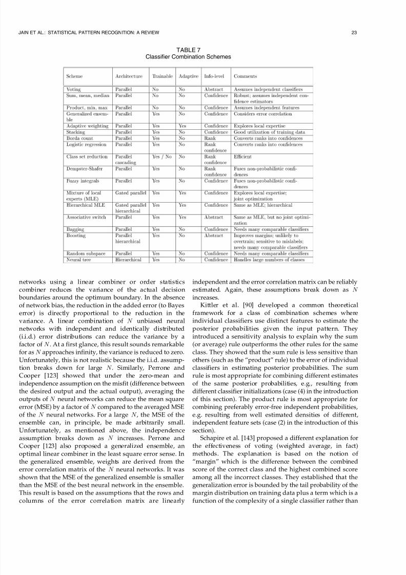
7/27/2019 Ja Indu in Mao Review
http://slidepdf.com/reader/full/ja-indu-in-mao-review 20/34
networks using a linear combiner or order statisticscombiner reduces the variance of the actual decision boundaries around the optimum boundary. In the absenceof network bias, the reduction in the added error (to Bayeserror) is directly proportional to the reduction in thevariance. A linear combination of x unbiased neuralnetworks with independent and identically distributed(i.i.d.) error distributions can reduce the variance by afactor of x . At a first glance, this result sounds remarkablefor as x approaches infinity, the variance is reduced to zero.Unfortunately, this is not realistic because the i.i.d. assump-tion breaks down for large x . Similarly, Perrone andCooper [123] showed that under the zero-mean andindependence assumption on the misfit (difference betweenthe desired output and the actual output), averaging theoutputs of x neural networks can reduce the mean squareerror (MSE) by a factor of x compared to the averaged MSEof the x neural networks. For a large x , the MSE of theensemble can, in principle, be made arbitrarily small.Unfortunately, as mentioned above, the independenceassumption breaks down as x increases. Perrone andCooper [123] also proposed a generalized ensemble, anoptimal linear combiner in the least square error sense. Inthe generalized ensemble, weights are derived from theerror correlation matrix of the x neural networks. It wasshown that the MSE of the generalized ensemble is smallerthan the MSE of the best neural network in the ensemble.This result is based on the assumptions that the rows and
columns of the error correlation matrix are linearly
independent and the error correlation matrix can be reliablyestimated. Again, these assumptions break down as x increases.
Kittler et al. [90] developed a common theoreticalframework for a class of combination schemes whereindividual classifiers use distinct features to estimate theposterior probabilities given the input pattern. Theyintroduced a sensitivity analysis to explain why the sum(or average) rule outperforms the other rules for the sameclass. They showed that the sum rule is less sensitive thanothers (such as the ªproductº rule) to the error of individualclassifiers in estimating posterior probabilities. The sumrule is most appropriate for combining different estimatesof the same posterior probabilities, e.g., resulting fromdifferent classifier initializations (case (4) in the introductionof this section). The product rule is most appropriate forcombining preferably error-free independent probabilities,e.g. resulting from well estimated densities of different,independent feature sets (case (2) in the introduction of thissection).
Schapire et al. [143] proposed a different explanation forthe effectiveness of voting (weighted average, in fact)methods. The explanation is based on the notion of ªmarginº which is the difference between the combinedscore of the correct class and the highest combined scoreamong all the incorrect classes. They established that thegeneralization error is bounded by the tail probability of themargin distribution on training data plus a term which is a
function of the complexity of a single classifier rather than
JAIN ET AL.: STATISTICAL PATTERN RECOGNITION: A REVIEW 23
TABLE 7Classifier Combination Schemes
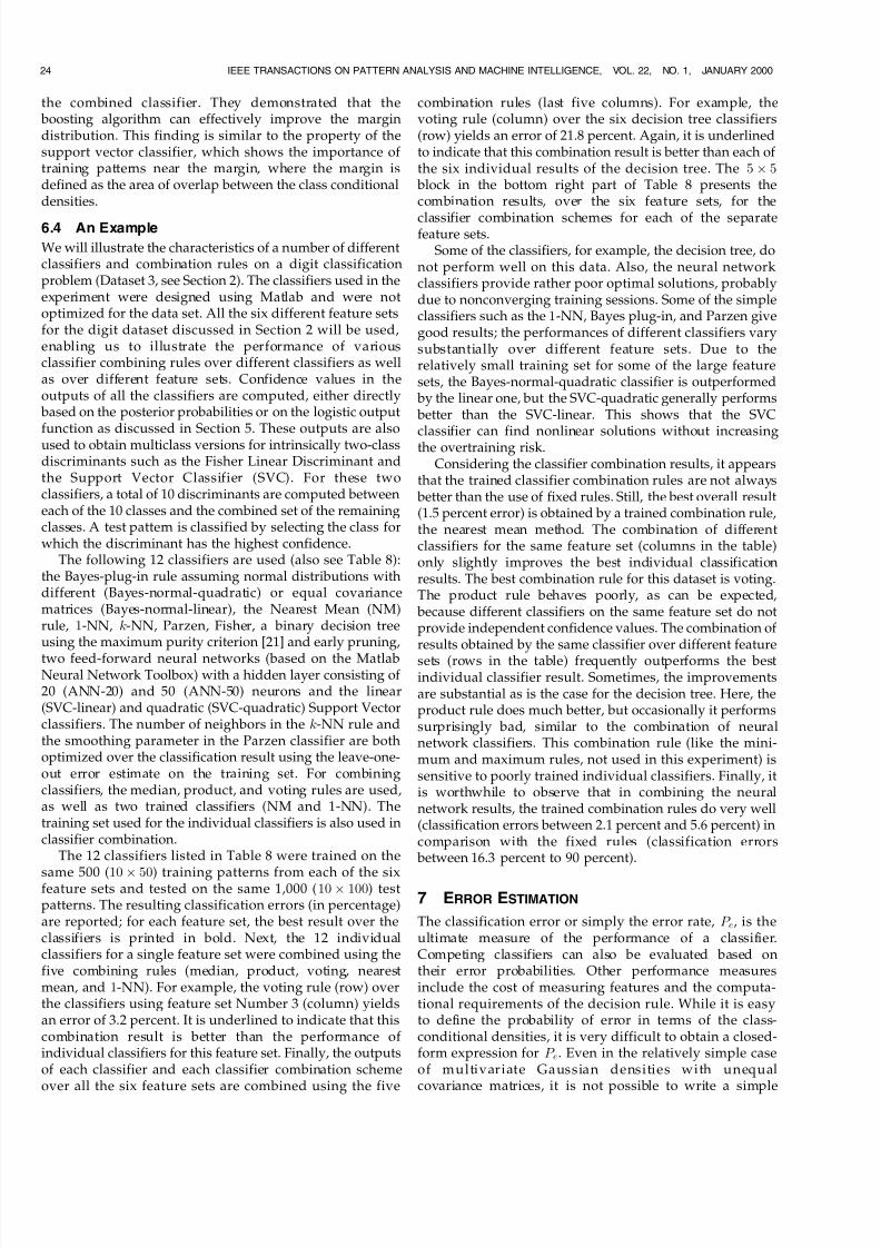
7/27/2019 Ja Indu in Mao Review
http://slidepdf.com/reader/full/ja-indu-in-mao-review 21/34
the combined classifier. They demonstrated that the boosting algorithm can effectively improve the margindistribution. This finding is similar to the property of thesupport vector classifier, which shows the importance of training patterns near the margin, where the margin isdefined as the area of overlap between the class conditionaldensities.
6.4 An Example
We will illustrate the characteristics of a number of differentclassifiers and combination rules on a digit classificationproblem (Dataset 3, see Section 2). The classifiers used in theexperiment were designed using Matlab and were notoptimized for the data set. All the six different feature setsfor the digit dataset discussed in Section 2 will be used,enabling us to illustrate the performance of variousclassifier combining rules over different classifiers as wellas over different feature sets. Confidence values in theoutputs of all the classifiers are computed, either directly based on the posterior probabilities or on the logistic outputfunction as discussed in Section 5. These outputs are alsoused to obtain multiclass versions for intrinsically two-classdiscriminants such as the Fisher Linear Discriminant andthe Support Vector Classifier (SVC). For these twoclassifiers, a total of 10 discriminants are computed betweeneach of the 10 classes and the combined set of the remainingclasses. A test pattern is classified by selecting the class forwhich the discriminant has the highest confidence.
The following 12 classifiers are used (also see Table 8):the Bayes-plug-in rule assuming normal distributions withdifferent (Bayes-normal-quadratic) or equal covariancematrices (Bayes-normal-linear), the Nearest Mean (NM)rule, I-NN, k-NN, Parzen, Fisher, a binary decision treeusing the maximum purity criterion [21] and early pruning,
two feed-forward neural networks (based on the MatlabNeural Network Toolbox) with a hidden layer consisting of 20 (ANN-20) and 50 (ANN-50) neurons and the linear(SVC-linear) and quadratic (SVC-quadratic) Support Vectorclassifiers. The number of neighbors in the k-NN rule andthe smoothing parameter in the Parzen classifier are bothoptimized over the classification result using the leave-one-out error estimate on the training set. For combiningclassifiers, the median, product, and voting rules are used,as well as two trained classifiers (NM and 1-NN). Thetraining set used for the individual classifiers is also used inclassifier combination.
The 12 classifiers listed in Table 8 were trained on the
same 500 (IH Â SH) training patterns from each of the sixfeature sets and tested on the same 1,000 (IH Â IHH) testpatterns. The resulting classification errors (in percentage)are reported; for each feature set, the best result over theclassifiers is printed in bold. Next, the 12 individualclassifiers for a single feature set were combined using thefive combining rules (median, product, voting, nearestmean, and I-NN). For example, the voting rule (row) overthe classifiers using feature set Number 3 (column) yieldsan error of 3.2 percent. It is underlined to indicate that thiscombination result is better than the performance of individual classifiers for this feature set. Finally, the outputsof each classifier and each classifier combination scheme
over all the six feature sets are combined using the five
combination rules (last five columns). For example, thevoting rule (column) over the six decision tree classifiers(row) yields an error of 21.8 percent. Again, it is underlinedto indicate that this combination result is better than each of the six individual results of the decision tree. The S Â S
block in the bottom right part of Table 8 presents thecombination results, over the six feature sets, for the
classifier combination schemes for each of the separatefeature sets.
Some of the classifiers, for example, the decision tree, donot perform well on this data. Also, the neural networkclassifiers provide rather poor optimal solutions, probablydue to nonconverging training sessions. Some of the simpleclassifiers such as the I-NN, Bayes plug-in, and Parzen givegood results; the performances of different classifiers varysubstantially over different feature sets. Due to therelatively small training set for some of the large featuresets, the Bayes-normal-quadratic classifier is outperformed by the linear one, but the SVC-quadratic generally performs better than the SVC-linear. This shows that the SVC
classifier can find nonlinear solutions without increasingthe overtraining risk.Considering the classifier combination results, it appears
that the trained classifier combination rules are not always better than the use of fixed rules. Still, the best overall result(1.5 percent error) is obtained by a trained combination rule,the nearest mean method. The combination of differentclassifiers for the same feature set (columns in the table)only slightly improves the best individual classificationresults. The best combination rule for this dataset is voting.The product rule behaves poorly, as can be expected, because different classifiers on the same feature set do notprovide independent confidence values. The combination of results obtained by the same classifier over different featuresets (rows in the table) frequently outperforms the bestindividual classifier result. Sometimes, the improvementsare substantial as is the case for the decision tree. Here, theproduct rule does much better, but occasionally it performssurprisingly bad, similar to the combination of neuralnetwork classifiers. This combination rule (like the mini-mum and maximum rules, not used in this experiment) issensitive to poorly trained individual classifiers. Finally, itis worthwhile to observe that in combining the neuralnetwork results, the trained combination rules do very well(classification errors between 2.1 percent and 5.6 percent) incomparison with the fixed rules (classification errors between 16.3 percent to 90 percent).
7 ERROR ESTIMATION
The classification error or simply the error rate, e, is theultimate measure of the performance of a classifier.Competing classifiers can also be evaluated based ontheir error probabilities. Other performance measuresinclude the cost of measuring features and the computa-tional requirements of the decision rule. While it is easyto define the probability of error in terms of the class-conditional densities, it is very difficult to obtain a closed-form expression for e. Even in the relatively simple caseof multivariate Gaussian densities with unequal
covariance matrices, it is not possible to write a simple
24 IEEE TRANSACTIONS ON PATTERN ANALYSIS AND MACHINE INTELLIGENCE, VOL. 22, NO. 1, JANUARY 2000

7/27/2019 Ja Indu in Mao Review
http://slidepdf.com/reader/full/ja-indu-in-mao-review 22/34
analytical expression for the error rate. If an analyticalexpression for the error rate was available, it could beused, for a given decision rule, to study the behavior of e as a function of the number of features, true parametervalues of the densities, number of training samples, andprior class probabilities. For consistent training rules thevalue of e approaches the Bayes error for increasingsample sizes. For some families of distributions tight bounds for the Bayes error may be obtained [7]. For finite
sample sizes and unknown distributions, however, such bounds are impossible [6], [41].
In practice, the error rate of a recognition system must beestimated from all the available samples which are split intotraining and test sets [70]. The classifier is first designedusing training samples, and then it is evaluated based on itsclassification performance on the test samples. The percen-tage of misclassified test samples is taken as an estimate of the error rate. In order for this error estimate to be reliablein predicting future classification performance, not onlyshould the training set and the test set be sufficiently large, but the training samples and the test samples must beindependent. This requirement of independent training and
test samples is still often overlooked in practice.An important point to keep in mind is that the error
estimate of a classifier, being a function of the specifictraining and test sets used, is a random variable. Given aclassifier, suppose ( is the number of test samples (out of a total of n) that are misclassified. It can be shown that theprobability density function of ( has a binomial distribu-tion. The maximum-likelihood estimate, e, of e is given by e (an, with i e e and e eI À ean.Thus, e is an unbiased and consistent estimator. Because e is a random variable, a confidence interval is associated
with it. Suppose n PSH and ( SH then e HXP and a95 percent confidence interval of e is HXISY HXPS. The
confidence interval, which shrinks as the number n of test
samples increases, plays an important role in comparingtwo competing classifiers, g I and g P. Suppose a total of 100 test samples are available and g I and g P misclassify 10and 13, respectively, of these samples. Is classifier g I betterthan g P? The 95 percent confidence intervals for the trueerror probabilities of these classifiers are HXHRY HXIT andHXHTY HXPH, respectively. Since these confidence intervalsoverlap, we cannot say that the performance of g I willalways be superior to that of g P. This analysis is somewhatpessimistic due to positively correlated error estimates based on the same test set [137].
How should the available samples be split to formtraining and test sets? If the training set is small, then theresulting classifier will not be very robust and will have alow generalization ability. On the other hand, if the test setis small, then the confidence in the estimated error rate will be low. Various methods that are commonly used toestimate the error rate are summarized in Table 9. Thesemethods differ in how they utilize the available samples astraining and test sets. If the number of available samples isextremely large (say, 1 million), then all these methods arelikely to lead to the same estimate of the error rate. Forexample, while it is well known that the resubstitutionmethod provides an optimistically biased estimate of theerror rate, the bias becomes smaller and smaller as the ratioof the number of training samples per class to thedimensionality of the feature vector gets larger and larger.There are no good guidelines available on how to divide theavailable samples into training and test sets; Fukunaga [58]provides arguments in favor of using more samples fortesting the classifier than for designing the classifier. Nomatter how the data is split into training and test sets, itshould be clear that different random splits (with thespecified size of training and test sets) will result in
different error estimates.
JAIN ET AL.: STATISTICAL PATTERN RECOGNITION: A REVIEW 25
TABLE 8Error Rates (in Percentage) of Different Classifiers and Classifier Combination Schemes

7/27/2019 Ja Indu in Mao Review
http://slidepdf.com/reader/full/ja-indu-in-mao-review 23/34
Fig. 9 shows the classification error of the Bayes plug-inlinear classifier on the digit dataset as a function of thenumber of training patterns. The test set error graduallyapproaches the training set error (resubstitution error) asthe number of training samples increases. The relativelylarge difference between these two error rates for 100training patterns per class indicates that the bias in thesetwo error estimates can be further reduced by enlarging thetraining set. Both the curves in this figure represent theaverage of 50 experiments in which training sets of thegiven size are randomly drawn; the test set of 1,000 patternsis fixed.
The holdout, leave-one-out, and rotation methods areversions of the cross-validation approach. One of themain disadvantages of cross-validation methods, espe-cially for small sample size situations, is that not all theavailable n samples are used for training the classifier.Further, the two extreme cases of cross validation, holdout method and leave-one-out method, suffer from eitherlarge bias or large variance, respectively. To overcomethis limitation, the bootstrap method [48] has beenproposed to estimate the error rate. The bootstrap methodresamples the available patterns with replacement togenerate a number of ªfakeº data sets (typically, severalhundred) of the same size as the given training set. Thesenew training sets can be used not only to estimate the bias of the resubstitution estimate, but also to defineother, so called bootstrap estimates of the error rate.Experimental results have shown that the bootstrapestimates can outperform the cross validation estimates
and the resubstitution estimates of the error rate [82].
In many pattern recognition applications, it is notadequate to characterize the performance of a classifier bya single number, e, which measures the overall error rateof a system. Consider the problem of evaluating afingerprint matching system, where two different yetrelated error rates are of interest. The False AcceptanceRate (FAR) is the ratio of the number of pairs of differentfingerprints that are incorrectly matched by a given systemto the total number of match attempts. The False Reject Rate(FRR) is the ratio of the number of pairs of the samefingerprint that are not matched by a given system to thetotal number of match attempts. A fingerprint matchingsystem can be tuned (by setting an appropriate threshold onthe matching score) to operate at a desired value of FAR.However, if we try to decrease the FAR of the system, thenit would increase the FRR and vice versa. The ReceiverOperating Characteristic (ROC) Curve [107] is a plot of FARversus FRR which permits the system designer to assess theperformance of the recognition system at various operatingpoints (thresholds in the decision rule). In this sense, ROCprovides a more comprehensive performance measure than,say, the equal error rate of the system (where FRR = FAR).Fig. 10 shows the ROC curve for the digit dataset where theBayes plug-in linear classifier is trained on 100 patterns perclass. Examples of the use of ROC analysis are combiningclassifiers [170] and feature selection [99].
In addition to the error rate, another useful perfor-
mance measure of a classifier is its reject rate. Suppose a
test pattern falls near the decision boundary between the
two classes. While the decision rule may be able to
correctly classify such a pattern, this classification will be
26 IEEE TRANSACTIONS ON PATTERN ANALYSIS AND MACHINE INTELLIGENCE, VOL. 22, NO. 1, JANUARY 2000
TABLE 9Error Estimation Methods

7/27/2019 Ja Indu in Mao Review
http://slidepdf.com/reader/full/ja-indu-in-mao-review 24/34
made with a low confidence. A better alternative would
be to reject these doubtful patterns instead of assigning
them to one of the categories under consideration. How
do we decide when to reject a test pattern? For the Bayes
decision rule, a well-known reject option is to reject a
pattern if its maximum a posteriori probability is below a
threshold; the larger the threshold, the higher the reject
rate. Invoking the reject option reduces the error rate; the
larger the reject rate, the smaller the error rate. This
relationship is represented as an error-reject trade-off
curve which can be used to set the desired operating
point of the classifier. Fig. 11 shows the error-reject curve
for the digit dataset when a Bayes plug-in linear classifier
is used. This curve is monotonically non-increasing, since
rejecting more patterns either reduces the error rate or
keeps it the same. A good choice for the reject rate is
based on the costs associated with reject and incorrect
decisions (See [66] for an applied example of the use of
error-reject curves).
8 UNSUPERVISED CLASSIFICATION
In many applications of pattern recognition, it is extremelydifficult or expensive, or even impossible, to reliably label a
training sample with its true category. Consider, forexample, the application of land-use classification in remotesensing. In order to obtain the ªground truthº information(category for each pixel) in the image, either the specific siteassociated with the pixel should be visited or its categoryshould be extracted from a Geographical InformationSystem, if one is available. Unsupervised classificationrefers to situations where the objective is to constructdecision boundaries based on unlabeled training data.Unsupervised classification is also known as data clusteringwhich is a generic label for a variety of procedures designedto find natural groupings, or clusters, in multidimensionaldata, based on measured or perceived similarities among
the patterns [81]. Category labels and other information
about the source of the data influence the interpretation of the clustering, not the formation of the clusters.
Unsupervised classification or clustering is a verydifficult problem because data can reveal clusters withdifferent shapes and sizes (see Fig. 12). To compound theproblem further, the number of clusters in the data oftendepends on the resolution (fine vs. coarse) with which weview the data. One example of clustering is the detectionand delineation of a region containing a high density of patterns compared to the background. A number of functional definitions of a cluster have been proposedwhich include: 1) patterns within a cluster are more similarto each other than are patterns belonging to different
clusters and 2) a cluster consists of a relatively high densityof points separated from other clusters by a relatively lowdensity of points. Even with these functional definitions of acluster, it is not easy to come up with an operationaldefinition of clusters. One of the challenges is to select anappropriate measure of similarity to define clusters which,in general, is both data (cluster shape) and contextdependent.
Cluster analysis is a very important and useful techni-que. The speed, reliability, and consistency with which aclustering algorithm can organize large amounts of dataconstitute overwhelming reasons to use it in applicationssuch as data mining [88], information retrieval [17], [25],
image segmentation [55], signal compression and coding[1], and machine learning [25]. As a consequence, hundredsof clustering algorithms have been proposed in theliterature and new clustering algorithms continue toappear. However, most of these algorithms are based onthe following two popular clustering techniques: iterativesquare-error partitional clustering and agglomerative hier-archical clustering. Hierarchical techniques organize data ina nested sequence of groups which can be displayed in theform of a dendrogram or a tree. Square-error partitionalalgorithms attempt to obtain that partition which minimizesthe within-cluster scatter or maximizes the between-clusterscatter. To guarantee that an optimum solution has been
obtained, one has to examine all possible partitions of the n
JAIN ET AL.: STATISTICAL PATTERN RECOGNITION: A REVIEW 27
Fig. 10. The ROC curve of the Bayes plug-in linear classifier for the digit
dataset.
Fig. 9. Classification error of the Bayes plug-in linear classifier (equal
covariance matrices) as a function of the number of training samples
(learning curve) for the test set and the training set on the digit dataset.

7/27/2019 Ja Indu in Mao Review
http://slidepdf.com/reader/full/ja-indu-in-mao-review 25/34
d -dimensional patterns into u clusters (for a given u ),which is not computationally feasible. So, various heuristicsare used to reduce the search, but then there is no guaranteeof optimality.
Partitional clustering techniques are used more fre-quently than hierarchical techniques in pattern recognitionapplications, so we will restrict our coverage to partitionalmethods. Recent studies in cluster analysis suggest that auser of a clustering algorithm should keep the followingissues in mind: 1) every clustering algorithm will findclusters in a given dataset whether they exist or not; thedata should, therefore, be subjected to tests for clusteringtendency before applying a clustering algorithm, followed
by a validation of the clusters generated by the algorithm; 2)there is no ªbestº clustering algorithm. Therefore, a user isadvised to try several clustering algorithms on agiven dataset. Further, issues of data collection, datarepresentation, normalization, and cluster validity are asimportant as the choice of clustering strategy.
The problem of partitional clustering can be formallystated as follows: Given n patterns in a d -dimensionalmetric space, determine a partition of the patterns into u clusters, such that the patterns in a cluster are more similarto each other than to patterns in different clusters [81]. Thevalue of u may or may not be specified. A clusteringcriterion, either global or local, must be adopted. A global
criterion, such as square-error, represents each cluster by aprototype and assigns the patterns to clusters according tothe most similar prototypes. A local criterion forms clusters by utilizing local structure in the data. For example, clusterscan be formed by identifying high-density regions in thepattern space or by assigning a pattern and its k nearestneighbors to the same cluster.
Most of the partitional clustering techniques implicitlyassume continuous-valued feature vectors so that thepatterns can be viewed as being embedded in a metricspace. If the features are on a nominal or ordinal scale,Euclidean distances and cluster centers are not verymeaningful, so hierarchical clustering methods are nor-
mally applied. Wong and Wang [169] proposed a clustering
algorithm for discrete-valued data. The technique of conceptual clustering or learning from examples [108] can be used with patterns represented by nonnumeric orsymbolic descriptors. The objective here is to group patternsinto conceptually simple classes. Concepts are defined interms of attributes and patterns are arranged into a
hierarchy of classes described by concepts.In the following subsections, we briefly summarize the
two most popular approaches to partitional clustering:square-error clustering and mixture decomposition. Asquare-error clustering method can be viewed as aparticular case of mixture decomposition. We should alsopoint out the difference between a clustering criterion and aclustering algorithm. A clustering algorithm is a particularimplementation of a clustering criterion. In this sense, thereare a large number of square-error clustering algorithms,each minimizing the square-error criterion and differingfrom the others in the choice of the algorithmic parameters.Some of the well-known clustering algorithms are listed in
Table 10 [81].
8.1 Square-Error Clustering
The most commonly used partitional clustering strategy is based on the square-error criterion. The general objectiveis to obtain that partition which, for a fixed number of clusters, minimizes the square-error. Suppose that thegiven set of n patterns in d dimensions has somehow been partitioned into u clusters fg IY g PY Á Á Á Y g k such thatcluster g k has nk patterns and each pattern is in exactlyone cluster, so that
u kI nk n.
The mean vector, or center, of cluster g k is defined as thecentroid of the cluster, or
mmk I
nk
nk
I
k Y IR
where k is the th pattern belonging to cluster g k. The
square-error for cluster g k is the sum of the squaredEuclidean distances between each pattern in g k and itscluster center mmk. This square-error is also called thewithin-cluster variation
ePk
nk
I
k À mmk
k À mmk
X IS
The square-error for the entire clustering containing u
clusters is the sum of the within-cluster variations:
28 IEEE TRANSACTIONS ON PATTERN ANALYSIS AND MACHINE INTELLIGENCE, VOL. 22, NO. 1, JANUARY 2000
Fig. 11. Error-reject curve of the Bayes plug-in linear classifier for the
digit dataset.
Fig. 12. Clusters with different shapes and sizes.

7/27/2019 Ja Indu in Mao Review
http://slidepdf.com/reader/full/ja-indu-in-mao-review 26/34
i Pu u
kI
ePkX IT
The objective of a square-error clustering method is to find a
partition containing u clusters that minimizes i Pu for a
fixed u . The resulting partition has also been referred to as
the minimum variance partition. A general algorithm for
the iterative partitional clustering method is given below.Agorithm for iterative partitional clustering:
Step 1. Select an initial partition with K clusters. Repeatsteps 2 through 5 until the cluster membership stabilizes.
Step 2. Generate a new partition by assigning each patternto its closest cluster center.
Step 3. Compute new cluster centers as the centroids of theclusters.
Step 4. Repeat steps 2 and 3 until an optimum value of thecriterion function is found.
Step 5. Adjust the number of clusters by merging andsplitting existing clusters or by removing small, oroutlier, clusters.
The above algorithm, without step 5, is also known as theu -means algorithm. The details of the steps in this algorithmmust either be supplied by the user as parameters or beimplicitly hidden in the computer program. However, thesedetails are crucial to the success of the program. A bigfrustration in using clustering programs is the lack of guidelinesavailableforchoosingu ,initialpartition,updatingthe partition, adjusting the number of clusters, and thestopping criterion [8].
The simple u -means partitional clustering algorithmdescribed above is computationally efficient and gives
surprisingly good results if the clusters are compact,hyperspherical in shape and well-separated in the featurespace. If the Mahalanobis distance is used in defining thesquared error in (16), then the algorithm is even able todetect hyperellipsoidal shaped clusters. Numerousattempts have been made to improve the performance of the basic u -means algorithm by 1) incorporating a fuzzycriterion function [15], resulting in a fuzzy u -means (or
-means) algorithm, 2) using genetic algorithms, simulated
annealing, deterministic annealing, and tabu search to
JAIN ET AL.: STATISTICAL PATTERN RECOGNITION: A REVIEW 29
TABLE 10Clustering Algorithms

7/27/2019 Ja Indu in Mao Review
http://slidepdf.com/reader/full/ja-indu-in-mao-review 27/34
optimize the resulting partition [110], [139], and 3) mappingit onto a neural network [103] for possibly efficientimplementation. However, many of these so-calledenhancements to the u -means algorithm are computation-ally demanding and require additional user-specifiedparameters for which no general guidelines are available. Judd et al. [88] show that a combination of algorithmic
enhancements to a square-error clustering algorithm anddistribution of the computations over a network of workstations can be used to cluster hundreds of thousandsof multidimensional patterns in just a few minutes.
It is interesting to note how seemingly different conceptsfor partitional clustering can lead to essentially the samealgorithm. It is easy to verify that the generalized Lloydvector quantization algorithm used in the communicationand compression domain is equivalent to the u -meansalgorithm. A vector quantizer (VQ) is described as acombination of an encoder and a decoder. A d -dimensionalVQ consists of two mappings: an encoder which maps theinput alphabet e to the channel symbol set w, and a
decoder which maps the channel symbol set w to theoutput alphabet e, i.e., yy X e 3w and v X w3 e.A distortion measure hyyY yy specifies the cost associatedwith quantization, where yy yy. Usually, an optimalquantizer minimizes the average distortion under a sizeconstraint on w. Thus, the problem of vector quantizationcan be posed as a clustering problem, where the number of clusters u is now the size of the output alphabet,e X fyyY IY F F F Y u , and the goal is to find a quantization(referred to as a partition in the u -means algorithm) of thed -dimensional feature space which minimizes the averagedistortion (mean square error) of the input patterns. Vectorquantization has been widely used in a number of compression and coding applications, such as speechwaveform coding, image coding, etc., where only thesymbols for the output alphabet or the cluster centers aretransmitted instead of the entire signal [67], [32]. Vectorquantization also provides an efficient tool for densityestimation [68]. A kernel-based approach (e.g., a mixture of Gaussian kernels, where each kernel is placed at a clustercenter) can be used to estimate the probability density of thetraining samples. A major issue in VQ is the selection of theoutput alphabet size. A number of techniques, such as theminimum description length (MDL) principle [138], can beused to select this parameter (see Section 8.2). Thesupervised version of VQ is called learning vector quantiza-tion (LVQ) [92].
8.2 Mixture Decomposition
Finite mixtures are a flexible and powerful probabilisticmodeling tool. In statistical pattern recognition, the mainuse of mixtures is in defining formal (i.e., model-based)approaches to unsupervised classification [81]. The reason behind this is that mixtures adequately model situationswhere each pattern has been produced by one of a set of alternative (probabilistically modeled) sources [155]. Never-theless, it should be kept in mind that strict adherence tothis interpretation is not required: mixtures can also be seenas a class of models that are able to represent arbitrarilycomplex probability density functions. This makes mixtures
also well suited for representing complex class-conditional
densities in supervised learning scenarios (see [137] andreferences therein). Finite mixtures can also be used as afeature selection tool [127].
8.2.1 Basic Definitions
Consider the following scheme for generating randomsamples. There are u random sources, each characterized
by a probability (mass or density) function myjm,parameterized by m, for m IYXXXYu . Each time a sampleis to be generated, we randomly choose one of thesesources, with probabilities fIYXXXYu , and then samplefrom the chosen source. The random variable defined bythis (two-stage) compound generating mechanism is char-acterized by a finite mixture distribution; formally, itsprobability function is
yjÂu u
mI
m myjmY IU
where each myjm is called a component, and
Âu fIY XXXY u Y IYXXXYu ÀI. It is usually assumed thatall the components have the same functional form; forexample, they are all multivariate Gaussian. Fitting amixture model to a set of observations y fyIY XXXYynconsists of estimating the set of mixture parameters that best describe this data. Although mixtures can be built frommany different types of components, the majority of theliterature focuses on Gaussian mixtures [155].
The two fundamental issues arising in mixture fittingare: 1) how to estimate the parameters defining the mixturemodel and 2) how to estimate the number of components[159]. For the first question, the standard answer is theexpectation-maximization (EM) algorithm (which, under mild
conditions, converges to the maximum likelihood (ML)estimate of the mixture parameters); several authors havealso advocated the (computationally demanding) Markovchain Monte-Carlo (MCMC) method [135]. The secondquestion is more difficult; several techniques have beenproposed which are summarized in Section 8.2.3. Note thatthe output of the mixture decomposition is as good as thevalidity of the assumed component distributions.
8.2.2 EM Algorithm
The expectation-maximization algorithm interprets thegiven observations y as incomplete data, with the missingpart being a set of labels associated with yY
z fzIY XXXYzu X
Missing variable z z I YXXXYz
u indicates which of the u
components generated yy; if it was the mth component,then z
m I and z H, for T m [155]. In the presence of
both y and z, the (complete) log-likelihood can be written as
v Âu YyY zÀ Á
n
jI
u
mI
z jm log m my jjmh i
Yu
I
IX
IVThe EM algorithm proceeds by alternatively applying thefollowing two steps:
30 IEEE TRANSACTIONS ON PATTERN ANALYSIS AND MACHINE INTELLIGENCE, VOL. 22, NO. 1, JANUARY 2000

7/27/2019 Ja Indu in Mao Review
http://slidepdf.com/reader/full/ja-indu-in-mao-review 28/34
. E-step: Compute the conditional expectation of thecomplete log-likelihood (given y and the currentparameter estimate, Â
u ). Since (18) is linear in themissing variables, the E-step for mixtures reduces tothe computation of the conditional expectation of themissing variables: wY
m i z m j Â
u Yy.. M-step: Update the parameter estimates:
ÂIu rg mxÂu Âu Y Â
u For the mixing probabilities, this becomes
Im I
n
n
I
wYm Y m IY PY Á Á Á Y u À IX IW
In the Gaussian case, each m consists of a meanvector and a covariance matrix which are updatedusing weighted versions (with weights I
m ) of thestandard ML estimates [155].
The main difficulties in using EM for mixture modelfitting, which are current research topics, are: its localnature, which makes it critically dependent on initialization;the possibility of convergence to a point on the boundary of the parameter space with unbounded likelihood (i.e., one of the m approaches zero with the corresponding covariance becoming arbitrarily close to singular).
8.2.3 Estimating the Number of Components
The ML criterion can not be used to estimate the number of mixture components because the maximized likelihood is anondecreasing function of u , thereby making it useless as amodel selection criterion (selecting a value for u in thiscase). This is a particular instance of the identifiabilityproblem where the classical (1P-based) hypothesis testing
cannot be used because the necessary regularity conditionsare not met [155]. Several alternative approaches that have been proposed are summarized below.
EM-based approaches use the (fixed u ) EM algorithm toobtain a sequence of parameter estimates for a range of values of u , f Âu Y u u minYXXXYu mx; the estimate of u is then defined as the minimizer of some cost function,
u rg minu g Âu Y u
Y u u minYXXXYu mx
n oX PH
Most often, this cost function includes the maximized log-likelihood function plus an additional term whose role is topenalize large values of u . An obvious choice in this class is
to use the minimum description length (MDL) criterion [10][138], but several other model selection criteria have beenproposed: Schwarz's Bayesian inference criterion (BIC), theminimum message length (MML) criterion, and Akaike'sinformation criterion (AIC) [2], [148], [167].
Resampling-based schemes and cross-validation-typeapproaches have also been suggested; these techniques are(computationally) much closer to stochastic algorithms thanto the methods in the previous paragraph. Stochasticapproaches generally involve Markov chain Monte Carlo(MCMC) [135] sampling and are far more computationallyintensive than EM. MCMC has been used in two differentways: to implement model selection criteria to actually
estimate u ; and, with a more ªfully Bayesian flavorº, to
sample from the full a posteriori distribution where u isincluded as an unknown. Despite their formal appeal, wethink that MCMC-based techniques are still far too compu-tationally demanding to be useful in pattern recognitionapplications.
Fig. 13 shows an example of mixture decomposition,where u is selected using a modified MDL criterion [51].
The data consists of 800 two-dimensional patterns distrib-uted over three Gaussian components; two of the compo-nents have the same mean vector but different covariancematrices and that is why one dense cloud of points is insideanother cloud of rather sparse points. The level curvecontours (of constant Mahalanobis distance) for the trueunderlying mixture and the estimated mixture are super-imposed on the data. For details, see [51]. Note that aclustering algorithm such as u -means will not be able toidentify these three components, due to the substantialoverlap of two of these components.
9 DISCUSSION
In its early stage of development, statistical pattern recogni-tion focused mainly on the core of the discipline: TheBayesian decision rule and its various derivatives (such aslinear and quadratic discriminant functions), density estima-tion, the curse of dimensionality problem, and errorestimation. Due to the limited computing power availablein the 1960s and 1970s, statistical pattern recognitionemployed relatively simple techniques which were appliedto small-scale problems.
Since the early 1980s, statistical pattern recognition hasexperienced a rapid growth. Its frontiers have beenexpanding in many directions simultaneously. This rapid
expansion is largely driven by the following forces.1. Increasing interaction and collaboration among
different disciplines, including neural networks,machine learning, statistics, mathematics, computerscience, and biology. These multidisciplinary effortshave fostered new ideas, methodologies, and tech-niques which enrich the traditional statistical patternrecognition paradigm.
2. The prevalence of fast processors, the Internet, largeand inexpensive memory and storage. The advancedcomputer technology has made it possible toimplement complex learning, searching and optimi-zation algorithms which was not feasible a few
decades ago. It also allows us to tackle large-scalereal world pattern recognition problems which mayinvolve millions of samples in high dimensionalspaces (thousands of features).
3. Emerging applications, such as data mining anddocument taxonomy creation and maintenance.These emerging applications have brought newchallenges that foster a renewed interest in statisticalpattern recognition research.
4. Last, but not the least, the need for a principled,rather than ad hoc approach for successfully solvingpattern recognition problems in a predictable way.For example, many concepts in neural networks,
which were inspired by biological neural networks,
JAIN ET AL.: STATISTICAL PATTERN RECOGNITION: A REVIEW 31

7/27/2019 Ja Indu in Mao Review
http://slidepdf.com/reader/full/ja-indu-in-mao-review 29/34
can be directly treated in a principled way instatistical pattern recognition.
9.1 Frontiers of Pattern Recognition
Table 11 summarizes several topics which, in our opinion,are at the frontiers of pattern recognition. As we can seefrom Table 11, many fundamental research problems instatistical pattern recognition remain at the forefront even
as the field continues to grow. One such example, modelselection (which is an important issue in avoiding the curseof dimensionality), has been a topic of continued researchinterest. A common practice in model selection relies oncross-validation (rotation method), where the best model isselected based on the performance on the validation set.Since the validation set is not used in training, this method
does not fully utilize the precious data for training which isespecially undesirable when the training data set is small.To avoid this problem, a number of model selectionschemes [71] have been proposed, including Bayesianmethods [14], minimum description length (MDL) [138],Akaike information criterion (AIC) [2] and marginalizedlikelihood [101], [159]. Various other regularization schemeswhich incorporate prior knowledge about model structureand parameters have also been proposed. Structural riskminimization based on the notion of VC dimension has also been used for model selection where the best model is theone with the best worst-case performance (upper bound onthe generalization error) [162]. However, these methods donot reduce the complexity of the search for the best model.Typically, the complexity measure has to be evaluated forevery possible model or in a set of prespecified models.Certain assumptions (e.g., parameter independence) areoften made in order to simplify the complexity evaluation.Model selection based on stochastic complexity has beenapplied to feature selection in both supervised learning andunsupervised learning [159] and pruning in decision
32 IEEE TRANSACTIONS ON PATTERN ANALYSIS AND MACHINE INTELLIGENCE, VOL. 22, NO. 1, JANUARY 2000
Fig.13. Mixture Decomposition Example.
TABLE 11Frontiers of Pattern Recognition

7/27/2019 Ja Indu in Mao Review
http://slidepdf.com/reader/full/ja-indu-in-mao-review 30/34
trees [106]. In the latter case, the best number of clusters isalso automatically determined.
Another example is mixture modeling using EM algo-rithm (see Section 8.2), which was proposed in 1977 [36],and which is now a very popular approach for densityestimation and clustering [159], due to the computingpower available today.
Over the recent years, a number of new concepts andtechniques have also been introduced. For example, themaximum margin objective was introduced in the contextof support vector machines [23] based on structural riskminimization theory [162]. A classifier with a large marginseparating two classes has a small VC dimension, whichyields a good generalization performance. Many successfulapplications of SVMs have demonstrated the superiority of this objective function over others [72]. It is found that the boosting algorithm [143] also improves the margin dis-tribution. The maximum margin objective can be consid-ered as a special regularized cost function, where theregularizer is the inverse of the margin between the two
classes. Other regularized cost functions, such as weightdecay and weight elimination, have also been used in thecontext of neural networks.
Due to the introduction of SVMs, linear and quadraticprogramming optimization techniques are once again beingextensively studied for pattern classification. Quadraticprogramming is credited for leading to the nice propertythat the decision boundary is fully specified by boundarypatterns, while linear programming with the vI norm or theinverse of the margin yields a small set of features when theoptimal solution is obtained.
The topic of local decision boundary learning has alsoreceived a lot of attention. Its primary emphasis is on usingpatterns near the boundary of different classes to construct
or modify the decision boundary. One such an example isthe boosting algorithm and its variation (AdaBoost) wheremisclassified patterns, mostly near the decision boundary,are subsampled with higher probabilities than correctlyclassified patterns to form a new training set for trainingsubsequent classifiers. Combination of local experts is alsorelated to this concept, since local experts can learn localdecision boundaries more accurately than global methods.In general, classifier combination could refine decision boundary such that its variance with respect to Bayesdecision boundary is reduced, leading to improvedrecognition accuracy [158].
Sequential data arise in many real world problems, such
as speech and on-line handwriting. Sequential patternrecognition has, therefore, become a very important topicin pattern recognition. Hidden Markov Models (HMM),have been a popular statistical tool for modeling andrecognizing sequential data, in particular, speech data[130], [86]. A large number of variations and enhancementsof HMMs have been proposed in the literature [12],including hybrids of HMMs and neural networks, input-output HMMs, weighted transducers, variable-durationHMMs, Markov switching models, and switching state-space models.
The growth in sensor technology and computingpower has enriched the availability of data in several
ways. Real world objects can now be represented by
many more measurements and sampled at high rates. Asphysical objects have a finite complexity, these measure-ments are generally highly correlated. This explains whymodels using spatial and spectral correlation in images,or the Markov structure in speech, or subspace ap-proaches in general, have become so important; theycompress the data to what is physically meaningful,
thereby improving the classification accuracy simulta-neously.
Supervised learning requires that every training sample be labeled with its true category. Collecting a large amountof labeled data can sometimes be very expensive. Inpractice, we often have a small amount of labeled dataand a large amount of unlabeled data. How to make use of unlabeled data for training a classifier is an importantproblem. SVM has been extended to perform semisuper-vised learning [13].
Invariant pattern recognition is desirable in manyapplications, such as character and face recognition. Earlyresearch in statistical pattern recognition did emphasize
extraction of invariant features which turns out to be a verydifficult task. Recently, there has been some activity indesigning invariant recognition methods which do notrequire invariant features. Examples are the nearestneighbor classifier using tangent distance [152] anddeformable template matching [84]. These approaches onlyachieve invariance to small amounts of linear transforma-tions and nonlinear deformations. Besides, they arecomputationally very intensive. Simard et al. [153] pro-posed an algorithm named Tangent-Prop to minimize thederivative of the classifier outputs with respect to distortionparameters, i.e., to improve the invariance property of theclassifier to the selected distortion. This makes the trainedclassifier computationally very efficient.
It is well-known that the human recognition processrelies heavily on context, knowledge, and experience. Theeffectiveness of using contextual information in resolvingambiguity and recognizing difficult patterns in the majordifferentiator between recognition abilities of human beingsand machines. Contextual information has been success-fully used in speech recognition, OCR, and remote sensing[173]. It is commonly used as a postprocessing step tocorrect mistakes in the initial recognition, but there is arecent trend to bring contextual information in the earlierstages (e.g., word segmentation) of a recognition system[174]. Context information is often incorporated through theuse of compound decision theory derived from Bayes
theory or Markovian models [175]. One recent, successfulapplication is the hypertext classifier [176] where therecognition of a hypertext document (e.g., a web page)can be dramatically improved by iteratively incorporatingthe category information of other documents that point to orare pointed by this document.
9.2 Concluding Remarks
Watanabe [164] wrote in the preface of the 1972 book heedited, entitled Frontiers of Pattern Recognition, that ªPatternrecognition is a fast-moving and proliferating discipline. Itis not easy to form a well-balanced and well-informedsummary view of the newest developments in this field. It
is still harder to have a vision of its future progress.º
JAIN ET AL.: STATISTICAL PATTERN RECOGNITION: A REVIEW 33

7/27/2019 Ja Indu in Mao Review
http://slidepdf.com/reader/full/ja-indu-in-mao-review 31/34
ACKNOWLEDGMENTS
The authors would like to thank the anonymous reviewers,
and Drs. Roz Picard, Tin Ho, and Mario Figueiredo for their
critical and constructive comments and suggestions. The
authors are indebted to Dr. Kevin Bowyer for his careful
review and to his students for their valuable feedback. The
authors are also indebted to following colleagues for theirvaluable assistance in preparing this manuscript: Elzbieta
Pekalska, Dick de Ridder, David Tax, Scott Connell, Aditya
Vailaya, Vincent Hsu, Dr. Pavel Pudil, and Dr. Patrick Flynn.
REFERENCES
[1] H.M. Abbas and M.M. Fahmy, ªNeural Networks for MaximumLikelihood Clustering,º Signal Processing, vol. 36, no. 1, pp. 111-126, 1994.
[2] H. Akaike, ªA New Look at Statistical Model Identification,º IEEETrans. Automatic Control, vol. 19, pp. 716-723, 1974.
[3] S. Amari, T.P. Chen, and A. Cichocki, ªStability Analysis of Learning Algorithms for Blind Source Separation,º Neural Net-works, vol. 10, no. 8, pp. 1,345-1,351, 1997.
[4] J.A. Anderson, ªLogistic Discrimination,º Handbook of Statistics. P.R. Krishnaiah and L.N. Kanal, eds., vol. 2, pp. 169-191,Amsterdam: North Holland, 1982.
[5] J. Anderson, A. Pellionisz, and E. Rosenfeld, Neurocomputing 2:Directions for Research. Cambridge Mass.: MIT Press, 1990.
[6] A. Antos, L. Devroye, and L. Gyorfi, ªLower Bounds for BayesError Estimation,º IEEE Trans. Pattern Analysis and MachineIntelligence, vol. 21, no. 7, pp. 643-645, July 1999.
[7] H. Avi-Itzhak and T. Diep, ªArbitrarily Tight Upper and LowerBounds on the Bayesian Probability of Error,º IEEE Trans. Pattern
Analysis and Machine Intelligence, vol. 18, no. 1, pp. 89-91, Jan. 1996.[8] E. Backer, Computer-Assisted Reasoning in Cluster Analysis. Prentice
Hall, 1995.[9] R. Bajcsy and S. Kovacic, ªMultiresolution Elastic Matching,º
Computer Vision Graphics Image Processing, vol. 46, pp. 1-21, 1989.[10] A. Barron, J. Rissanen, and B. Yu, ªThe Minimum Description
Length Principle in Coding and Modeling,º IEEE Trans. Informa-
tion Theory, vol. 44, no. 6, pp. 2,743-2,760, Oct. 1998.[11] A. Bell and T. Sejnowski, ªAn Information-Maximization Ap-proach to Blind Separation,º Neural Computation, vol. 7, pp. 1,004-1,034, 1995.
[12] Y. Bengio, ªMarkovian Models for Sequential Data,º NeuralComputing Surveys, vol. 2, pp. 129-162, 1999. http://www.icsi.
berkeley.edu/~jagota/NCS.[13] K.P. Bennett, ªSemi-Supervised Support Vector Machines,º Proc.
Neural Information Processing Systems, Denver, 1998.[14] J. Bernardo and A. Smith, Bayesian Theory. John Wiley & Sons,
1994.[15] J.C. Bezdek, Pattern Recognition with Fuzzy Objective Function
Algorithms. New York: Plenum Press, 1981.[16] Fuzzy Models for Pattern Recognition: Methods that Search for
Structures in Data. J.C. Bezdek and S.K. Pal, eds., IEEE CS Press,1992.
[17] S.K. Bhatia and J.S. Deogun, ªConceptual Clustering in Informa-
tion Retrieval,º IEEE Trans. Systems, Man, and Cybernetics, vol. 28,no. 3, pp. 427-436, 1998.[18] C.M. Bishop, Neural Networks for Pattern Recognition. Oxford:
Clarendon Press, 1995.[19] A.L. Blum and P. Langley, ªSelection of Relevant Features and
Examples in Machine Learning,º Artificial Intelligence, vol. 97,nos. 1-2, pp. 245-271, 1997.
[20] I. Borg and P. Groenen, Modern Multidimensional Scaling, Berlin:Springer-Verlag, 1997.
[21] L. Breiman, ªBagging Predictors,º Machine Learning, vol. 24, no. 2,pp. 123-140, 1996.
[22] L. Breiman, J.H. Friedman, R.A. Olshen, and C.J. Stone, Classifica-tion and Regression Trees. Wadsworth, Calif., 1984.
[23] C.J.C. Burges, ªA Tutorial on Support Vector Machines for PatternRecognition,º Data Mining and Knowledge Discovery, vol. 2, no. 2,pp. 121-167, 1998.
[24] J. Cardoso, ªBlind Signal Separation: Statistical Principles,º Proc.
IEEE, vol. 86, pp. 2,009-2,025, 1998.
[25] C. Carpineto and G. Romano, ªA Lattice Conceptual ClusteringSystem and Its Application to Browsing Retrieval,º MachineLearning, vol. 24, no. 2, pp. 95-122, 1996.
[26] G. Castellano, A.M. Fanelli, and M. Pelillo, ªAn Iterative PruningAlgorithm for Feedforward Neural Networks,º IEEE Trans. NeuralNetworks, vol. 8, no. 3, pp. 519-531, 1997.
[27] C. Chatterjee and V.P. Roychowdhury, ªOn Self-OrganizingAlgorithms and Networks for Class-Separability Features,º IEEETrans. Neural Networks, vol. 8, no. 3, pp. 663-678, 1997.
[28] B. Cheng and D.M. Titterington, ªNeural Networks: A Reviewfrom Statistical Perspective,º Statistical Science, vol. 9, no. 1, pp. 2-54, 1994.
[29] H. Chernoff, ªThe Use of Faces to Represent Points ink-Dimensional Space Graphically,º J. Am. Statistical Assoc.,vol. 68, pp. 361-368, June 1973.
[30] P.A. Chou, ªOptimal Partitioning for Classification and Regres-sion Trees,º IEEE Trans. Pattern Analysis and Machine Intelligence,vol. 13, no. 4, pp. 340-354, Apr. 1991.
[31] P. Comon, ªIndependent Component Analysis, a New Concept?,ºSignal Processing, vol. 36, no. 3, pp. 287-314, 1994.
[32] P.C. Cosman, K.L. Oehler, E.A. Riskin, and R.M. Gray, ªUsingVector Quantization for Image Processing,º Proc. IEEE, vol. 81,pp. 1,326-1,341, Sept. 1993.
[33] T.M. Cover, ªGeometrical and Statistical Properties of Systems of Linear Inequalities with Applications in Pattern Recognition,º
IEEE Trans. Electronic Computers, vol. 14, pp. 326-334, June 1965.[34] T.M. Cover, ªThe Best Two Independent Measurements are notthe Two Best,º IEEE Trans. Systems, Man, and Cybernetics, vol. 4,pp. 116-117, 1974.
[35] T.M. Cover and J.M. Van Campenhout, ªOn the PossibleOrderings in the Measurement Selection Problem,º IEEE Trans.Systems, Man, and Cybernetics, vol. 7, no. 9, pp. 657-661, Sept. 1977.
[36] A. Dempster, N. Laird, and D. Rubin, ªMaximum Likelihood fromIncomplete Data via the (EM) Algorithm,º J. Royal Statistical Soc.,vol. 39, pp. 1-38, 1977.
[37] H. Demuth and H.M. Beale, Neural Network Toolbox for Use with Matlab. version 3, Mathworks, Natick, Mass., 1998.
[38] D. De Ridder and R.P.W. Duin, ªSammon's Mapping UsingNeural Networks: Comparison,º Pattern Recognition Letters, vol. 18,no. 11-13, pp. 1,307-1,316, 1997.
[39] P.A. Devijver and J. Kittler, Pattern Recognition: A Statistical Approach. London: Prentice Hall, 1982.
[40] L. Devroye, ªAutomatic Pattern Recognition: A Study of theProbability of Error,º IEEE Trans. Pattern Analysis and MachineIntelligence, vol. 10, no. 4, pp. 530-543, 1988.
[41] L. Devroye, L. Gyorfi, and G. Lugosi, A Probabilistic Theory of Pattern Recognition. Berlin: Springer-Verlag, 1996.
[42] A. Djouadi and E. Bouktache, ªA Fast Algorithm for the Nearest-Neighbor Classifier,º IEEE Trans. Pattern Analysis and MachineIntelligence, vol. 19, no. 3, pp. 277-282, 1997.
[43] H. Drucker, C. Cortes, L.D. Jackel, Y. Lecun, and V. Vapnik,ªBoosting and Other Ensemble Methods,º Neural Computation,vol. 6, no. 6, pp. 1,289-1,301, 1994.
[44] R.O. Duda and P.E. Hart, Pattern Classification and Scene Analysis,New York: John Wiley & Sons, 1973.
[45] R.O. Duda, P.E. Hart, and D.G. Stork, Pattern Classification andScene Analysis. second ed., New York: John Wiley & Sons, 2000.
[46] R.P.W. Duin, ªA Note on Comparing Classifiers,º Pattern
Recognition Letters, vol. 17, no. 5, pp. 529-536, 1996.[47] R.P.W. Duin, D. De Ridder, and D.M.J. Tax, ªExperiments with a
Featureless Approach to Pattern Recognition,º Pattern RecognitionLetters, vol. 18, nos. 11-13, pp. 1,159-1,166, 1997.
[48] B. Efron, The Jackknife, the Bootstrap and Other Resampling Plans.Philadelphia: SIAM, 1982.
[49] U. Fayyad, G. Piatetsky-Shapiro, and P. Smyth, ªKnowledgeDiscovery and Data Mining: Towards a Unifying Framework,ºProc. Second Int'l Conf. Knowledge Discovery and Data Mining, Aug.1999.
[50] F. Ferri, P. Pudil, M. Hatef, and J. Kittler, ªComparative Study of Techniques for Large Scale Feature Selection,º Pattern Recognitionin Practice IV, E. Gelsema and L. Kanal, eds., pp. 403-413, 1994.
[51] M. Figueiredo, J. Leitao, and A.K. Jain, ªOn Fitting MixtureModels,º Energy Minimization Methods in Computer Vision andPattern Recognition. E. Hancock and M. Pellillo, eds., Springer-
Verlag, 1999.
34 IEEE TRANSACTIONS ON PATTERN ANALYSIS AND MACHINE INTELLIGENCE, VOL. 22, NO. 1, JANUARY 2000

7/27/2019 Ja Indu in Mao Review
http://slidepdf.com/reader/full/ja-indu-in-mao-review 32/34
[52] Y. Freund and R. Schapire, ªExperiments with a New BoostingAlgorithm,º Proc. 13th Int'l Conf. Machine Learning, pp. 148-156,1996.
[53] J.H. Friedman, ªExploratory Projection Pursuit,º J. Am. Statistical Assoc., vol. 82, pp. 249-266, 1987.
[54] J.H. Friedman, ªRegularized Discriminant Analysis,º J. Am.Statistical Assoc., vol. 84, pp. 165-175, 1989.
[55] H. Frigui and R. Krishnapuram, ªA Robust CompetitiveClustering Algorithm with Applications in Computer Vision,º
IEEE Trans. Pattern Analysis and Machine Intelligence, vol. 21,no. 5, pp. 450-465, 1999.
[56] K.S. Fu, Syntactic Pattern Recognition and Applications. EnglewoodCliffs, N.J.: Prentice-Hall, 1982.
[57] K.S. Fu, ªA Step Towards Unification of Syntactic and StatisticalPattern Recognition,º IEEE Trans. Pattern Analysis and MachineIntelligence, vol. 5, no. 2, pp. 200-205, Mar. 1983.
[58] K. Fukunaga, Introduction to Statistical Pattern Recognition. seconded., New York: Academic Press, 1990.
[59] K. Fukunaga and R.R. Hayes, ªEffects of Sample Size inClassifier Design,º IEEE Trans. Pattern Analysis and MachineIntelligence, vol. 11, no. 8, pp. 873-885, Aug. 1989.
[60] K. Fukunaga and R.R. Hayes, ªThe Reduced Parzen Classifier,ºIEEE Trans. Pattern Analysis and Machine Intelligence, vol. 11, no. 4,pp. 423-425, Apr. 1989.
[61] K. Fukunaga and D.M. Hummels, ªLeave-One-Out Procedures forNonparametric Error Estimates,º IEEE Trans. Pattern Analysis and
Machine Intelligence, vol. 11, no. 4, pp. 421-423, Apr. 1989.[62] K. Fukushima, S. Miyake, and T. Ito, ªNeocognitron: A Neural
Network Model for a Mechanism of Visual Pattern Recognition,ºIEEE Trans. Systems, Man, and Cybernetics, vol. 13, pp. 826-834,1983.
[63] S.B. Gelfand, C.S. Ravishankar, and E.J. Delp, ªAn IterativeGrowing and Pruning Algorithm for Classification Tree Design,ºIEEE Trans. Pattern Analysis and Machine Intelligence, vol. 13, no. 2,pp. 163-174, Feb. 1991.
[64] S. Geman, E. Bienenstock, and R. Doursat, ªNeural Networks andthe Bias/Variance Dilemma,º Neural Computation, vol. 4, no. 1, pp.1-58, 1992.
[65] C. Glymour, D. Madigan, D. Pregibon, and P. Smyth, ªStatisticalThemes and Lessons for Data Mining,º Data Mining and KnowledgeDiscovery, vol. 1, no. 1, pp. 11-28, 1997.
[66] M. Golfarelli, D. Maio, and D. Maltoni, ªOn the Error-RejectTrade-Off in Biometric Verification System,º IEEE Trans. Pattern
Analysis and Machine Intelligence, vol. 19, no. 7, pp. 786-796, July1997.
[67] R.M. Gray, ªVector Quantization,º IEEE ASSP, vol. 1, pp. 4-29,Apr. 1984.
[68] R.M. Gray and R.A. Olshen, ªVector Quantization and DensityEstimation,º Proc. Int'l Conf. Compression and Complexity of Sequences, 1997. http://www-isl.stanford.edu/~gray/compression.html.
[69] U. Grenander, General Pattern Theory. Oxford Univ. Press, 1993.[70] D.J. Hand, ªRecent Advances in Error Rate Estimation,º Pattern
Recognition Letters, vol. 4, no. 5, pp. 335-346, 1986.[71] M.H. Hansen and B. Yu, ªModel Selection and the Principle of
Minimum Description Length,º technical report, Lucent Bell Lab,Murray Hill, N.J., 1998.
[72] M.A. Hearst, ªSupport Vector Machines,º IEEE Intelligent Systems,pp. 18-28, July/Aug. 1998.
[73] S. Haykin, Neural Networks, A Comprehensive Foundation. seconded., Englewood Cliffs, N.J.: Prentice Hall, 1999.
[74] T. K. Ho, J.J. Hull, and S.N. Srihari, ªDecision Combination inMultiple Classifier Systems,º IEEE Trans. Pattern Analysis and
Machine Intelligence, vol. 16, no. 1, pp. 66-75, 1994.[75] T.K. Ho, ªThe Random Subspace Method for Constructing
Decision Forests,º IEEE Trans. Pattern Analysis and MachineIntelligence, vol. 20, no. 8, pp. 832-844, Aug. 1998.
[76] J.P. Hoffbeck and D.A. Landgrebe, ªCovariance Matrix Estimationand Classification with Limited Training Data,º IEEE Trans.Pattern Analysis and Machine Intelligence, vol. 18, no. 7, pp. 763-767,
July 1996.[77] A. Hyvarinen, ªSurvey on Independent Component Analysis,º
Neural Computing Surveys, vol. 2, pp. 94-128, 1999. http://www.icsi.berkeley.edu/~jagota/NCS.
[78] A. Hyvarinen and E. Oja, ªA Fast Fixed-Point Algorithm forIndependent Component Analysis,º Neural Computation, vol. 9,
no. 7, pp. 1,483-1,492, Oct. 1997.
[79] R.A. Jacobs, M.I. Jordan, S.J. Nowlan, and G.E. Hinton, ªAdaptiveMixtures of Local Experts,º Neural Computation, vol. 3, pp. 79-87,1991.
[80] A.K. Jain and B. Chandrasekaran, ªDimensionality and SampleSize Considerations in Pattern Recognition Practice,º Handbook of Statistics. P.R. Krishnaiah and L.N. Kanal, eds., vol. 2, pp. 835-855,Amsterdam: North-Holland, 1982.
[81] A.K. Jain and R.C. Dubes, Algorithms for Clustering Data. Engle-wood Cliffs, N.J.: Prentice Hall, 1988.
[82] A.K. Jain, R.C. Dubes, and C.-C. Chen, ªBootstrap Techniques forError Estimation,º IEEE Trans. Pattern Analysis and MachineIntelligence, vol. 9, no. 5, pp. 628-633, May 1987.
[83] A.K. Jain, J. Mao, and K.M. Mohiuddin, ªArtificial NeuralNetworks: A Tutorial,º Computer, pp. 31-44, Mar. 1996.
[84] A. Jain, Y. Zhong, and S. Lakshmanan, ªObject Matching UsingDeformable Templates,º IEEE Trans. Pattern Analysis and MachineIntelligence, vol. 18, no. 3, Mar. 1996.
[85] A.K. Jain and D. Zongker, ªFeature Selection: Evaluation,Application, and Small Sample Performance,º IEEE Trans. Pattern
Analysis and Machine Intelligence, vol. 19, no. 2, pp. 153-158, Feb.1997.
[86] F. Jelinek, Statistical Methods for Speech Recognition. MIT Press,1998.
[87] M.I. Jordan and R.A. Jacobs, ªHierarchical Mixtures of Expertsand the EM Algorithm,º Neural Computation, vol. 6, pp. 181-214,1994.
[88] D. Judd, P. Mckinley, and A.K. Jain, ªLarge-Scale Parallel DataClustering,º IEEE Trans. Pattern Analysis and Machine Intelligence,vol. 20, no. 8, pp. 871-876, Aug. 1998.
[89] L.N. Kanal, ªPatterns in Pattern Recognition: 1968-1974,º IEEETrans. Information Theory, vol. 20, no. 6, pp. 697-722, 1974.
[90] J. Kittler, M. Hatef, R.P.W. Duin, and J. Matas, ªOn CombiningClassifiers,º IEEE Trans. Pattern Analysis and Machine Intelligence,vol. 20, no. 3, pp. 226-239, 1998.
[91] R.M. Kleinberg, ªStochastic Discrimination,º Annals of Math. and Artificial Intelligence, vol. 1, pp. 207-239, 1990.
[92] T. Kohonen, Self-Organizing Maps. Springer Series in InformationSciences, vol. 30, Berlin, 1995.
[93] A. Krogh and J. Vedelsby, ªNeural Network Ensembles, CrossValidation, and Active Learning,º Advances in Neural InformationProcessing Systems, G. Tesauro, D. Touretsky, and T. Leen, eds.,vol. 7, Cambridge, Mass.: MIT Press, 1995.
[94] L. Lam and C.Y. Suen, ªOptimal Combinations of Pattern
Classifiers,º Pattern Recognition Letters, vol. 16, no. 9, pp. 945-954,1995.
[95] Y. Le Cun, B. Boser, J.S. Denker, D. Henderson, R.E. Howard,W. Hubbard, and L.D. Jackel, ªBackpropagation Applied toHandwritten Zip Code Recognition,º Neural Computation, vol. 1,pp. 541-551, 1989.
[96] T.W. Lee, Independent Component Analysis. Dordrech: KluwerAcademic Publishers, 1998.
[97] C. Lee and D.A. Landgrebe, ªFeature Extraction Based onDecision Boundaries,º IEEE Trans. Pattern Analysis and MachineIntelligence, vol. 15, no. 4, pp. 388-400, 1993.
[98] B. Lerner, H. Guterman, M. Aladjem, and I. Dinstein, ªAComparative Study of Neural Network Based Feature ExtractionParadigms,º Pattern Recognition Letters vol. 20, no. 1, pp. 7-14, 1999
[99] D.R. Lovell, C.R. Dance, M. Niranjan, R.W. Prager, K.J. Dalton,and R. Derom, ªFeature Selection Using Expected AttainableDiscrimination,º Pattern Recognition Letters, vol. 19, nos. 5-6,pp. 393-402, 1998.
[100] D. Lowe and A.R. Webb, ªOptimized Feature Extraction and theBayes Decision in Feed-Forward Classifier Networks,º IEEE Trans.Pattern Analysis and Machine Intelligence, vol. 13, no. 4, pp. 355-264,Apr. 1991.
[101] D.J.C. MacKay, ªThe Evidence Framework Applied to Classifica-tion Networks,º Neural Computation, vol. 4, no. 5, pp. 720-736,1992.
[102] J.C. Mao and A.K. Jain, ªArtificial Neural Networks for FeatureExtraction and Multivariate Data Projection,º IEEE Trans. NeuralNetworks, vol. 6, no. 2, pp. 296-317, 1995.
[103] J. Mao, K. Mohiuddin, and A.K. Jain, ªParsimonious NetworkDesign and Feature Selection through Node Pruning,º Proc. 12thInt'l Conf. Pattern on Recognition, pp. 622-624, Oct. 1994.
[104] J.C. Mao and K.M. Mohiuddin, ªImproving OCR PerformanceUsing Character Degradation Models and Boosting Algorithm,º
Pattern Recognition Letters, vol. 18, no. 11-13, pp. 1,415-1,419, 1997.
JAIN ET AL.: STATISTICAL PATTERN RECOGNITION: A REVIEW 35
7/27/2019 Ja Indu in Mao Review
http://slidepdf.com/reader/full/ja-indu-in-mao-review 33/34
[105] G. McLachlan, Discriminant Analysis and Statistical Pattern Recogni-tion. New York: John Wiley & Sons, 1992.
[106] M. Mehta, J. Rissanen, and R. Agrawal, ªMDL-Based DecisionTree Pruning,º Proc. First Int'l Conf. Knowledge Discovery inDatabases and Data Mining, Montreal, Canada Aug. 1995
[107] C.E. Metz, ªBasic Principles of ROC Analysis,º Seminars in Nuclear Medicine, vol. VIII, no. 4, pp. 283-298, 1978.
[108] R.S. Michalski and R.E. Stepp, ªAutomated Construction of Classifications: Conceptual Clustering versus Numerical Taxon-
omy,º IEEE Trans. Pattern Analysis and Machine Intelligence, vol. 5,pp. 396-410, 1983.
[109] D. Michie, D.J. Spiegelhalter, and C.C. Taylor, Machine Learning,Neural and Statistical Classification. New York: Ellis Horwood, 1994.
[110] S.K. Mishra and V.V. Raghavan, ªAn Empirical Study of thePerformance of Heuristic Methods for Clustering,º PatternRecognition in Practice. E.S. Gelsema and L.N. Kanal, eds., North-Holland, pp. 425-436, 1994.
[111] G. Nagy, ªState of the Art in Pattern Recognition,º Proc. IEEE, vol.56, pp. 836-862, 1968.
[112] G. Nagy, ªCandide's Practical Principles of Experimental PatternRecognition,º IEEE Trans. Pattern Analysis and Machine Intelligence,vol. 5, no. 2, pp. 199-200, 1983.
[113] R. Neal, Bayesian Learning for Neural Networks. New York: SpringVerlag, 1996.
[114] H. Niemann, ªLinear and Nonlinear Mappings of Patterns,ºPattern Recognition, vol. 12, pp. 83-87, 1980.
[115] K.L. Oehler and R.M. Gray, ªCombining Image Compression andClassification Using Vector Quantization,º IEEE Trans. Pattern
Analysis and Machine Intelligence, vol. 17, no. 5, pp. 461-473, 1995.[116] E. Oja, Subspace Methods of Pattern Recognition, Letchworth,
Hertfordshire, England: Research Studies Press, 1983.[117] E. Oja, ªPrincipal Components, Minor Components, and Linear
Neural Networks,º Neural Networks, vol. 5, no. 6, pp. 927-936.1992.
[118] E. Oja, ªThe Nonlinear PCA Learning Rule in IndependentComponent Analysis,º Neurocomputing, vol. 17, no.1, pp. 25-45,1997.
[119] E. Osuna, R. Freund, and F. Girosi, ªAn Improved TrainingAlgorithm for Support Vector Machines,º Proc. IEEE WorkshopNeural Networks for Signal Processing. J. Principe, L. Gile, N.Morgan, and E. Wilson, eds., New York: IEEE CS Press, 1997.
[120] Y. Park and J. Sklanski, ªAutomated Design of Linear Tree
Classifiers,º Pattern Recognition, vol. 23, no. 12, pp. 1,393-1,412,1990.[121] T. Pavlidis, Structural Pattern Recognition. New York: Springer-
Verlag, 1977.[122] L.I. Perlovsky, ªConundrum of Combinatorial Complexity,º
IEEE Trans. Pattern Analysis and Machine Intelligence, vol. 20,no. 6, pp. 666-670, 1998.
[123] M.P. Perrone and L.N. Cooper, ªWhen Networks Disagree:Ensemble Methods for Hybrid Neural Networks,º Neural Net-works for Speech and Image Processing. R.J. Mammone, ed.,Chapman-Hall, 1993.
[124] J. Platt, ªFast Training of Support Vector Machines UsingSequential Minimal Optimization,º Advances in Kernel MethodsÐ-Support Vector Learning. B. Scholkopf, C.J. C. Burges, and A.J.Smola, eds., Cambridge, Mass.: MIT Press, 1999.
[125] R. Picard, Affective Computing. MIT Press, 1997.[126] P. Pudil, J. Novovicova, and J. Kittler, ªFloating Search Methods
in Feature Selection,º Pattern Recognition Letters, vol. 15, no. 11,pp. 1,119-1,125, 1994.
[127] P. Pudil, J. Novovicova, and J. Kittler, ªFeature Selection Based onthe Approximation of Class Densities by Finite Mixtures of theSpecial Type,º Pattern Recognition, vol. 28, no. 9, pp. 1,389-1,398,1995.
[128] J.R. Quinlan, ªSimplifying Decision Trees,º Int'l J. Man-MachineStudies, vol. 27, pp. 221-234, 1987.
[129] J.R. Quinlan, C4.5: Programs for Machine Learning. San Mateo,Calif.: Morgan Kaufmann, 1993.
[130] L.R. Rabiner, ªA Tutorial on Hidden Markov Models andSelected Applications in Speech Recognition,º Proc. IEEE,vol. 77, pp. 257-286, Feb. 1989.
[131] S.J. Raudys and V. Pikelis, ªOn Dimensionality, Sample Size,Classification Error, and Complexity of Classification Algorithmsin Pattern Recognition,º IEEE Trans. Pattern Analysis and Machine
Intelligence, vol. 2, pp. 243-251, 1980.
[132] S.J. Raudys and A.K. Jain, ªSmall Sample Size Effects inStatistical Pattern Recognition: Recommendations for Practi-tioners,º IEEE Trans. Pattern Analysis and Machine Intelligence,vol. 13, no. 3, pp. 252-264, 1991.
[133] S. Raudys, ªEvolution and Generalization of a Single Neuron;Single-Layer Perceptron as Seven Statistical Classifiers,º NeuralNetworks, vol. 11, no. 2, pp. 283-296, 1998.
[134] S. Raudys and R.P.W. Duin, ªExpected Classification Error of theFisher Linear Classifier with Pseudoinverse Covariance Matrix,º
Pattern Recognition Letters, vol. 19, nos. 5-6, pp. 385-392, 1998.[135] S. Richardson and P. Green, ªOn Bayesian Analysis of Mixtures
with Unknown Number of Components,º J. Royal Statistical Soc.(B), vol. 59, pp. 731-792, 1997.
[136] B. Ripley, ªStatistical Aspects of Neural Networks,º Networks onChaos: Statistical and Probabilistic Aspects. U. Bornndorff-Nielsen, J.
Jensen, and W. Kendal, eds., Chapman and Hall, 1993.[137] B. Ripley, Pattern Recognition and Neural Networks. Cambridge,
Mass.: Cambridge Univ. Press, 1996.[138] J. Rissanen, Stochastic Complexity in Statistical Inquiry, Singapore:
World Scientific, 1989.
[139] K. Rose, ªDeterministic Annealing for Clustering, Compression,Classification, Regression and Related Optimization Problems,ºProc. IEEE, vol. 86, pp. 2,210-2,239, 1998.
[140] P.E. Ross, ªFlash of Genius,º Forbes, pp. 98-104, Nov. 1998.
[141] J.W. Sammon Jr., ªA Nonlinear Mapping for Data Structure
Analysis,º IEEE Trans. Computer, vol. l8, pp. 401-409, 1969.[142] R.E. Schapire, ªThe Strength of Weak Learnability,º Machine
Learning, vol. 5, pp. 197-227, 1990.
[143] R.E. Schapire, Y. Freund, P. Bartlett, and W.S. Lee, ªBoosting theMargin: A New Explanation for the Effectiveness of VotingMethods,º Annals of Statistics, 1999.
[144] B. SchoÈ lkopf, ªSupport Vector Learning,º Ph.D. thesis, TechnischeUniversitaÈt, Berlin, 1997.
[145] B. SchoÈ lkopf, A. Smola, and K.R. Muller, ªNonlinear Compo-nent Analysis as a Kernel Eigenvalue Problem,º NeuralComputation, vol. 10, no. 5, pp. 1,299-1,319, 1998.
[146] B. SchoÈ lkopf, K.-K. Sung, C.J.C. Burges, F. Girosi, P. Niyogi, T.Poggio, and V. Vapnik, ªComparing Support Vector Machineswith Gaussian Kernels to Radial Basis Function Classifiers,º IEEETrans. Signal Processing, vol. 45, no. 11, pp. 2,758-2,765, 1997.
[147] J. Schurmann, Pattern Classification: A Unified View of Statistical andNeural Approaches. New York: John Wiley & Sons, 1996.
[148] S. Sclove, ªApplication of the Conditional Population MixtureModel to Image Segmentation,º IEEE Trans. Pattern Recognitionand Machine Intelligence, vol. 5, pp. 428-433, 1983.
[149] I.K. Sethi and G.P.R. Sarvarayudu, ªHierarchical Classifier DesignUsing Mutual Information,º IEEE Trans. Pattern Recognition and
Machine Intelligence, vol. 1, pp. 194-201, Apr. 1979.[150] R. Setiono and H. Liu, ªNeural-Network Feature Selector,º IEEE
Trans. Neural Networks, vol. 8, no. 3, pp. 654-662, 1997.[151] W. Siedlecki and J. Sklansky, ªA Note on Genetic Algorithms for
Large-Scale Feature Selection,º Pattern Recognition Letters, vol. 10,pp. 335-347, 1989.
[152] P. Simard, Y. LeCun, and J. Denker, ªEfficient Pattern RecognitionUsing a New Transformation Distance,º Advances in NeuralInformation Processing Systems, 5, S.J. Hanson, J.D. Cowan, andC.L. Giles, eds., California: Morgan Kaufmann, 1993.
[153] P. Simard, B. Victorri, Y. LeCun, and J. Denker, ªTangent PropÐA
Formalism for Specifying Selected Invariances in an AdaptiveNetwork,º Advances in Neural Information Processing Systems, 4, J.E.Moody, S.J. Hanson, and R.P. Lippmann, eds., pp. 651-655,California: Morgan Kaufmann, 1992.
[154] P. Somol, P. Pudil, J. Novovicova, and P. Paclik, ªAdaptiveFloating Search Methods in Feature Selection,º Pattern RecognitionLetters, vol. 20, nos. 11, 12, 13, pp. 1,157-1,163, 1999.
[155] D. Titterington, A. Smith, and U. Makov, Statistical Analysis of Finite Mixture Distributions. Chichester, U.K.: John Wiley & Sons,1985.
[156] V. Tresp and M. Taniguchi, ªCombining Estimators Using Non-Constant Weighting Functions,º Advances in Neural InformationProcessing Systems, G. Tesauro, D.S. Touretzky, and T.K. Leen,eds., vol. 7, Cambridge, Mass.: MIT Press, 1995.
[157] G.V. Trunk, ªA Problem of Dimensionality: A Simple Example,ºIEEE Trans. Pattern Analysis and Machine Intelligence, vol. 1, no. 3,
pp. 306-307, July 1979.
36 IEEE TRANSACTIONS ON PATTERN ANALYSIS AND MACHINE INTELLIGENCE, VOL. 22, NO. 1, JANUARY 2000

7/27/2019 Ja Indu in Mao Review
http://slidepdf.com/reader/full/ja-indu-in-mao-review 34/34
[158] K. Tumer and J. Ghosh, ªAnalysis of Decision Boundaries inLinearly Combined Neural Classifiers,º Pattern Recognition, vol. 29,pp. 341-348, 1996.
[159] S. Vaithyanathan and B. Dom, ªModel Selection in UnsupervisedLearning with Applications to Document Clustering,º Proc. SixthInt'l Conf. Machine Learning, pp. 433-443, June 1999.
[160] M. van Breukelen, R.P.W. Duin, D.M.J. Tax, and J.E. den Hartog,ªHandwritten Digit Recognition by Combined Classifiers,ºKybernetika, vol. 34, no. 4, pp. 381-386, 1998.
[161] V.N. Vapnik, Estimation of Dependences Based on Empirical Data,Berlin: Springer-Verlag, 1982.[162] V.N. Vapnik, Statistical Learning Theory. New York: John Wiley &
Sons, 1998.[163] S. Watanabe, Pattern Recognition: Human and Mechanical. New
York: Wiley, 1985.[164] Frontiers of Pattern Recognition. S. Watanabe, ed., New York:
Academic Press, 1972.[165] A.R. Webb, ªMultidimensional Scaling by Iterative Majorization
Using Radial Basis Functions,º Pattern Recognition, vol. 28, no. 5,pp. 753-759, 1995.
[166] S.M. Weiss and C.A. Kulikowski, Computer Systems that Learn.California: Morgan Kaufmann Publishers, 1991.
[167] M. Whindham and A. Cutler, ªInformation Ratios for ValidatingMixture Analysis,º J. Am. Statistical Assoc., vol. 87, pp. 1,188-1,192,1992.
[168] D. Wolpert, ªStacked Generalization,º Neural Networks, vol. 5, pp.
241-259, 1992.[169] A.K.C. Wong and D.C.C. Wang, ªDECA: A Discrete-Valued DataClustering Algorithm,º IEEE Trans. Pattern Analysis and MachineIntelligence, vol. 1, pp. 342-349, 1979.
[170] K. Woods, W.P. Kegelmeyer Jr., and K. Bowyer, ªCombination of Multiple Classifiers Using Local Accuracy Estimates,º IEEE Trans.Pattern Analysis and Machine Intelligence, vol. 19, no. 4, pp. 405-410,Apr. 1997.
[171] Q.B. Xie, C.A. Laszlo, and R.K. Ward, ªVector QuantizationTechnique for Nonparametric Classifier Design,º IEEE Trans.Pattern Analysis and Machine Intelligence, vol. 15, no. 12, pp. 1,326-1,330, 1993.
[172] L. Xu, A. Krzyzak, and C.Y. Suen, ªMethods for CombiningMultiple Classifiers and Their Applications in HandwrittenCharacter Recognition,º IEEE Trans. Systems, Man, and Cybernetics,vol. 22, pp. 418-435, 1992.
[173] G.T. Toussaint, ªThe Use of Context in Pattern Recognition,º
Pattern Recognition, vol, 10, no. 3, pp. 189-204, 1978.[174] K. Mohiuddin and J. Mao, ªOptical Character Recognition,º WileyEncyclopedia of Electrical and Electronic Engineering. J.G. Webster,ed., vol. 15, pp. 226-236, John Wiley and Sons, Inc., 1999.
[175] R.M. Haralick, ªDecision Making in Context,º IEEE Trans.Pattern Analysis and Machine Intelligence, vol. 5, no. 4, pp. 417-418, Mar. 1983.
[176] S. Chakrabarti, B. Dom, and P. Idyk, ªEnhanced HypertextCategorization Using Hyperlinks,º ACM SIGMOD, Seattle, 1998.
Anil K. Jain is a university distinguishedprofessor in the Department of ComputerScience and Engineering at Michigan StateUniversity. His research interests include statis-tical pattern recognition, Markov random fields,texture analysis, neural networks, documentimage analysis, fingerprint matching and 3D
object recognition. He received best paperawards in 1987 and 1991 and certificates foroutstanding contributions in 1976, 1979, 1992,
and 1997 from the Pattern Recognition Society. He also received the1996 IEEE Transactions on Neural Networks Outstanding Paper Award.He was the editor-in-chief of the IEEE Transaction on Pattern Analysis and Machine Intelligence (1990-1994). He is the co-author of Algorithms for Clustering Data, has edited the book Real-Time Object Measurement and Classification, and co-edited the books, Analysis and Interpretation of Range Images, Markov Random Fields, Artificial Neural Networks and Pattern Recognition, 3D Object Recognition, and BIOMETRICS: Personal Identification in Networked Society. He received a Fulbright
Robert P.W. Duin studied applied physics atDelft University of Technology in the Nether-lands. In 1978, he received the PhD degree for athesis on the accuracy of statistical patternrecognizers. In his research, he included variousaspects of the automatic interpretation of mea-surements, learning systems, and classifiers.Between 1980 and 1990, he studied and devel-oped hardware architectures and software con-
figurations for interactive image analysis. Atpresent, he is an associate professor of the faculty of applied sciencesof Delft University of Technology. His present research interest is in thedesign and evaluation of learning algorithms for pattern recognitionapplications. This includes, in particular, neural network classifiers,support vector classifiers, and classifier combining strategies. Recently,he began studying the possibilities of relational methods for patternrecognition.
Jianchang Mao received the PhD degree incomputer science from Michigan State Univer-sity, East Lansing, in 1994. He is currently aresearch staff member at the IBM AlmadenResearch Center in San Jose, California. Hisresearch interests include pattern recognition,machine learning, neural networks, informationretrieval, web mining, document image analysis,
OCR and handwriting recognition, image proces-sing, and computer vision. He received thehonorable mention award from the Pattern Recognition Society in1993, and the 1996 IEEE Transactions on Neural Networks outstanding paper award. He also received two IBM Researchdivision awards in 1996 and 1998, and an IBM outstandingtechnical achievement award in 1997. He was a guest co-editorof a special issue of IEEE Transactions on Nueral Networks. Hehas served as an associate editor of IEEE Transactions on Neural Networks, and as an editorial board member for Pattern Analysisand Applications. He also served as a program committee memberfor several international conferences. He is a senior member of theIEEE.
JAIN ET AL.: STATISTICAL PATTERN RECOGNITION: A REVIEW 37