j. wang, s. huang, w. zuo, d. vrabie 2021. “occupant
TRANSCRIPT

1
J. Wang, S. Huang, W. Zuo, D. Vrabie 2021. “Occupant Preference-Aware Load 1
Scheduling for Resilient Communities.” Energy and Buildings, 252, pp. 111399. 2
https://doi.org/10.1016/j.enbuild.2021.111399 3
4
5
Occupant Preference-Aware Load Scheduling for Resilient Communities 6
Jing Wanga, Sen Huangb, Wangda Zuoa,c,*, Draguna Vrabieb 7
a University of Colorado Boulder, Department of Civil, Environmental and Architectural 8
Engineering, Boulder, CO 80309, United States 9
b Pacific Northwest National Laboratory, 902 Battelle Blvd, Richland, WA 99354, United States 10
c National Renewable Energy Laboratory, 15013 Denver West Parkway, Golden, CO 80401, 11
United States 12
13
14
Abstract 15
The load scheduling of resilient communities in the islanded mode is subject to many uncertainties 16
such as weather forecast errors and occupant behavior stochasticity. To date, it remains unclear 17
how occupant preferences affect the effectiveness of the load scheduling of resilient communities. 18
This paper proposes an occupant preference-aware load scheduler for resilient communities 19
operating in the islanded mode. The load scheduling framework is formulated as a model 20
predictive control problem. Based on this framework, a deterministic load scheduler is adopted as 21
the baseline. Then, a chance-constrained scheduler is proposed to address the occupant-induced 22
uncertainty in room temperature setpoints. Key resilience indicators are selected to quantify the 23
impacts of the uncertainties on community load scheduling. Finally, the proposed preference-24
aware scheduler is compared with the deterministic scheduler on a virtual testbed based on a real-25
world net-zero energy community in Florida, USA. Results show that the proposed scheduler 26
performs better in terms of serving the occupants’ thermal preference and reducing the required 27
* Corresponding author.
Email address: [email protected].
2
battery size, given the presence of the assumed stochastic occupant behavior. This work indicates 28
that it is necessary to consider the stochasticity of occupant behavior when designing optimal load 29
schedulers for resilient communities. 30
Keywords: Microgrid; Optimal load scheduling; Uncertainty; Occupant behavior; Resilient 31
community; Model predictive control. 32
Nomenclature 33
Parameters 𝐸𝑏𝑎𝑡𝑡 battery energy
𝑎 intercept coefficient for the logistic
regression model 𝑃𝑐ℎ
𝑡 battery charging power
𝑏 slope coefficient for the logistic regression
model 𝑃𝑐𝑟𝑖𝑡,𝑗
𝑡 scheduled critical loads
𝐸𝑏𝑎𝑡 upper limit of battery energy 𝑃𝑐𝑢𝑟𝑡𝑡 curtailed PV power
𝑒 mathematical constant 𝑃𝑑𝑖𝑠𝑡 battery discharging power
H MPC prediction horizon 𝑃ℎ𝑣𝑎𝑐𝑡 HVAC system (heat pump) total power
N simulation horizon 𝑃𝑙𝑜𝑎𝑑𝑡 total scheduled loads
𝑁𝑐𝑟𝑖𝑡 number of critical loads in each building 𝑃𝑚𝑜𝑑𝑢,𝑗𝑡 scheduled modulatable loads
𝑁𝑚𝑜𝑑𝑢 number of modulatable loads in each
building 𝑃𝑠ℎ𝑒𝑑,𝑗
𝑡 scheduled sheddable loads
𝑁𝑠ℎ𝑒𝑑 number of sheddable loads in each building 𝑃𝑠ℎ𝑖𝑓,𝑗𝑡 scheduled shiftable loads
𝑁𝑠ℎ𝑖𝑓 number of shiftable loads in each building 𝑃𝑝𝑣𝑡 PV power
𝑛𝑠ℎ𝑖𝑓,𝑗 average cycle time of each shiftable load 𝑟ℎ𝑣𝑎𝑐𝑡 speed ratio of the heat pump
𝑃𝑏𝑎𝑡 upper limit of battery power 𝑇𝑟𝑜𝑜𝑚 indoor air temperature
�̂�𝑐𝑟𝑖𝑡,𝑗𝑡 critical load data 𝑡𝑠ℎ𝑖𝑓,𝑗,𝑠 starting operation time of shiftable loads
𝑃ℎ𝑣𝑎𝑐,𝑛𝑜𝑚 HVAC system (heat pump) nominal power 𝑄𝑔𝑎𝑖𝑛𝑡 internal heat gain
𝑃𝑙𝑜𝑎𝑑
𝑡 predicted loads upper bound Binary Variables
�̂�𝑚𝑜𝑑𝑢,𝑗𝑡 modulatable load data 𝑢𝑠ℎ𝑒𝑑,𝑗
𝑡 binary decision variable for sheddable load
on/off status
�̂�𝑠ℎ𝑒𝑑,𝑗𝑡 sheddable load data 𝑣𝑠ℎ𝑖𝑓,𝑗
𝑡 binary variable for shiftable load starting
time
3
𝑃𝑠ℎ𝑖𝑓,𝑗,𝑎𝑣𝑔 average nominal power of each shiftable
load Abbreviations
𝑝 probability of setpoint-changing actions BAL building agent layer
𝑺𝑠ℎ𝑖𝑓,𝑗 scheduling matrix for each shiftable load CDF cumulative distribution function
𝑇𝑎𝑚𝑏𝑡 ambient outdoor temperature COL community operator layer
𝑇𝑟𝑜𝑜𝑚 lower room temperature bound DER distributed energy resource
𝑇𝑟𝑜𝑜𝑚 upper room temperature bound DR demand response
𝑄𝑠𝑜𝑙𝑡 solar irradiance HVAC heating, ventilation, and air-conditioning
𝛾 penalty coefficients KRI key resilience indicator
∆𝑡 timestep MPC model predictive control
𝜖, 𝜖𝑇 maximum constraint violation probability RC resistance-capacitance
𝜂𝑐ℎ battery charging efficiency RMSE Root Mean Square Error
𝜂𝑑𝑖𝑠 battery discharging efficiency SOC state of charge
𝜇𝑇𝑡 mean of room temperature error distribution PDF probability density function
𝜎𝑇𝑡
standard deviation of room temperature
error distribution PID proportional integral derivative
Continuous Variables PV photovoltaics
34
1 Introduction 35
Due to the increasing frequency of extreme weather events such as the 2021 Texas Power Crisis 36
[1], there is an emerging need for community resilience studies. Resilient communities refer to 37
those that can sustain disruptions and adapt to them quickly by continuing to operate without 38
sacrificing the occupants’ essential needs [2, 3]. Enabling technologies for resilient communities 39
often involve distributed energy resources (DERs) such as photovoltaics (PV) and electrical energy 40
storage (EES) systems. When disconnected from the main grid, the adoption of advanced control 41
techniques can help enhance community resilience. 42
As an advanced control technique, optimal load scheduling determines the operation schedules of 43
controllable devices in the community to achieve optimization objectives. For a resilient 44
community, typical controllable assets include the EES, PV, and thermostatically controllable 45
4
devices in buildings such as the heating, ventilation, and air-conditioning (HVAC) system. 46
Building plug loads that are sheddable, shiftable, or modulatable can also be considered flexible 47
loads in islanded circumstances [4]. The objectives of the load scheduling for resilient 48
communities often involve maximizing the self-consumption rate of locally generated PV energy, 49
minimizing PV curtailment, and minimizing the unserved ratio to critical loads. 50
It is important to account for uncertainties when designing a load scheduler for resilient 51
communities. Moreover, due to the limited amount of available PV generation during off-grid 52
scenarios, the uncertainties need to be more carefully dealt with to ensure a satisfying control 53
performance. Sources of uncertainties for a community load scheduling problem mainly lie in two 54
aspects: power generation and consumption. For renewable energy generation, weather forecast 55
errors play a prominent role in the cause of uncertainty. Whereas, for energy consumption, 56
occupant behavior stochasticity is a major source of uncertainty. 57
Much of existing load scheduling research has considered the uncertainty of weather forecasts [5–58
13]. Kou [5] proposed a comprehensive scheduling framework for residential building demand 59
response (DR) considering both day-ahead and real-time electricity markets. The results 60
demonstrated the effectiveness of the proposed approach for large-scale residential DR 61
applications under weather and consumer uncertainties. Garifi [13] adopted stochastic 62
optimization in a model predictive control (MPC)-based home energy management system. The 63
indoor thermal comfort is ensured at a high probability with uncertainty in the outdoor temperature 64
and solar irradiance forecasts. Faraji [6] proposed a hybrid learning-based method using an 65
artificial neural network to precisely predict the weather data, which eliminated the impact of 66
weather forecast uncertainties on the scheduling of microgrids. Similarly, in the authors’ previous 67
publication [7], normally distributed outdoor temperature and solar irradiance forecast errors were 68
introduced into the community control framework, which accounted for the uncertainties in the 69
weather forecasts. 70
However, the uncertainties from the power consumption perspective, especially the occupant 71
behavior uncertainty, is rarely accounted for in load scheduling research [14–18]. Some efforts to 72
integrate occupant behavior modeling can be found in studies of building optimal control [19–22]. 73
Aftab [19] used video-processing and machine-learning techniques to enable real-time building 74
occupancy recognition and prediction. This further facilitated the HVAC system operation control 75
5
to achieve building energy savings. Lim [20] solved a joint occupancy scheduling and occupancy-76
based HVAC control problem for the optimal room-booking (i.e., meeting scheduling) in 77
commercial and educational buildings. Both the occupancy status of each meeting room and the 78
HVAC control variables were decision variables. Mixed-integer linear programming was adopted 79
to optimally solve the optimization problem. 80
Notably, all of the preceding control work considered the stochasticity of building occupancy 81
schedules, but the integration of other types of occupant behavior into building optimal control is 82
not well studied in existing literature. Some researchers integrate the occupant thermal sensation 83
feedback into the MPC for buildings [23, 24]. For instance, Chen [23] integrated a dynamic thermal 84
sensation model into the MPC to help achieve energy savings using the HVAC control. For the 85
occupant sensation model, the predictive performance of certainty-equivalence MPC and chance-86
constrained MPC were compared. 87
To summarize, the literature review shows that current research mainly focuses on the load 88
scheduling of single buildings under grid-connected scenarios. There is a lack of research on the 89
optimal load scheduling of resilient communities informed by occupant behavior uncertainties in 90
the islanded mode. Given this gap, this paper proposes an occupant preference-aware load 91
scheduling framework for resilient communities in the islanded mode. The occupants’ thermal 92
preference for indoor air temperature will be reflected in the integration of thermostat adjustment 93
probabilistic models. The optimal load scheduling is formulated as an MPC problem, so the 94
stochastic thermostat-changing behavior will be regarded as the uncertainty in the MPC problem. 95
Different methods, such as the offset-free method and robust method, can be used to handle the 96
uncertainties in MPC problems [25]. The chance-constraint method, also known as the stochastic 97
MPC, was selected to deal with the uncertainty in occupant preference in our study. It allows the 98
violation of certain constraints at a predetermined probability. It thus enables a systematic trade-99
off between the control performance and the constraint violations [26]. The advantage of 100
addressing occupant preference uncertainty by using the chance-constraint method lies in the a 101
priori handling of the uncertainty, which does not require the extra error-prediction models needed 102
by other methods (i.e., offset free method), and thus simplifies the control problem [27]. Therefore, 103
less computational effort is required after the control design phase. Though it requires the 104

6
controller to know the estimated uncertainty distribution beforehand, the development of occupant 105
behavior probabilistic modeling will make knowing this less challenging. 106
In this work, we consider the load scheduling of a resilient community in islanded mode during 107
power outages. The goal is to study the impact of occupants’ thermal preference on the operation 108
of an islanded community. The load scheduling problem of the community will be solved using 109
an optimization-based hierarchical control framework. Occupant thermal preference will be 110
integrated through thermostat changing behavioral models to inform the development of the load 111
scheduler. The major contributions of this work include (1) a proposed new preference-aware load 112
scheduler for resilient communities, which assures better control performance related to satisfying 113
occupants’ thermal preferences and reducing the battery size; (2) the quantification of the impact 114
of occupant thermostat-changing behavior on resilient community optimal scheduling using 115
selected key resilience indicators (KRIs); and (3) the testing of the proposed scheduler on a high-116
fidelity virtual testbed for resilient communities. 117
The remainder of this paper is organized as follows: Section 2 details the research methodology. 118
Section 3 describes the controllable device models used in this work involving the building HVAC 119
models, load models, and battery models. Section 4 then discusses the deterministic versus 120
stochastic scheduler formulations and proposes a chance-constrained controller for preference-121
aware load scheduling of resilient communities. Section 5 applies the theoretical work to a case 122
study community and quantifies the impact of occupant preference uncertainty. Simulation results 123
and discussions are presented in this section. Finally, Section 6 concludes the paper by identifying 124
future work. 125
2 Methodology 126
In this section, we first introduce a hierarchical optimal control structure for resilient community 127
load scheduling. Based on the structure, a deterministic scheduler will be implemented as the 128
baseline. Further, we propose a research workflow to implement a stochastic preference-aware 129
scheduler for addressing uncertainties in occupant thermostat-changing behavior. KRIs are 130
proposed at the end of this section. 131

7
2.1 Hierarchical Optimal Control for Resilient Communities 132
In this study, we assume that the only energy resource accessible to the islanded community is on-133
site PV generation and the batteries for an extended period of more than 24 hours. In this problem 134
setting, in order to make full use of the limited amount of PV generation and satisfy the occupants’ 135
essential needs, the building loads need to be shifted or modulated. The battery works as a temporal 136
arbitrage for meeting the demand at night. In addition, the occupant thermal preference will affect 137
the energy consumption of the HVAC system through the stochastic thermostat-changing behavior. 138
To optimally control such a community, considering the above factors, we adopted a hierarchical 139
control structure. 140
As illustrated in Figure 1, two layers of control are formulated: a community operator layer (COL) 141
and a building agent layer (BAL). The COL optimally allocates the limited amount of the on-site 142
PV generation based on the load flexibility provided by each building. The calculated allowable 143
load for each building is then passed down to the BAL, where each building optimally schedules 144
its controllable devices (i.e., HVAC, battery, and controllable loads) to achieve its local 145
optimization goals. Both layers are formulated as MPC-based optimization problems. 146
147
Figure 1 The hierarchical optimal control structure for community operation. 148
The input of the hierarchical control involves the predicted PV generation data, outdoor air dry-149
bulb temperature, and solar irradiance. The PV generation data are used by the COL to determine 150
the optimal allocation among buildings. The temperature and irradiance data are used by the 151
HVAC models for updating the indoor room temperature predictions. The occupant behavior 152

8
affects the two layers differently. The COL uses building occupancy schedules to decide the 153
weights of different buildings during the PV allocation (details can be found in [7]). The BAL 154
considers occupant thermal preference to be the uncertainty in the indoor room temperature 155
prediction. 156
2.2 Proposed Workflow 157
Figure 2 depicts the workflow of this paper. A deterministic optimal load scheduler without the 158
occupant thermal preference uncertainty is implemented in the hierarchical control structure. 159
Further, to account for the uncertainties, we propose a chance-constrained controller. It is 160
developed based on the deterministic controller and involves an alteration of the room temperature 161
constraints, which accounts for the uncertainties in room temperature prediction errors caused by 162
the occupants’ thermostat-changing behavior. The Monte Carlo simulation method was adopted 163
to cover a wide range of simulation results. 164
165
Figure 2 Diagram of the proposed workflow. 166
Further, to reflect various styles of occupant behavior, three types of occupant thermostat-changing 167
models were adopted: low, medium, and high, which represent three levels of frequencies of the 168
thermostat-changing activities. Here, we assume that when the occupant decides to change the 169
indoor air temperature setpoint according to their preference, the predetermined optimal HVAC 170
equipment control setting at the current timestep will be overridden. Instead, a new control setting 171
will be calculated to achieve the occupants’ setpoint at the current timestep. At the next timestep, 172
the predetermined optimal setting will still be used if the occupant is not changing the setpoint 173
consecutively. 174

9
Finally, the optimal schedules determined by the chance-constrained controller and the 175
deterministic controller are tested on a high-fidelity virtual testbed [28] with respect to their 176
individual performances. KRIs such as the unserved load ratio, the required battery size, and the 177
unmet thermal preference hours were adopted to quantify the results. 178
The unserved load ratio in this paper is defined as the relative discrepancy between the served 179
load 𝑃𝑙𝑜𝑎𝑑𝑡 and the originally predicted load 𝑃𝑙𝑜𝑎𝑑
𝑡: 180
𝑈𝑛𝑠𝑒𝑟𝑣𝑒𝑑 𝑙𝑜𝑎𝑑 𝑟𝑎𝑡𝑖𝑜 =∑ (𝑃𝑙𝑜𝑎𝑑
𝑡− 𝑃𝑙𝑜𝑎𝑑
𝑡 )𝑁𝑡=1
∑ 𝑃𝑙𝑜𝑎𝑑
𝑡𝑁𝑡=1
, (1)
where 𝑁 is the MPC simulation horizon of 48 hours. The required battery size is obtained by 181
subtracting the minimum battery SOC from the maximum SOC. This gives us a sense of how much 182
of the battery capacity has been used under different scenarios. Finally, we define the unmet 183
thermal preference hours metric for the cumulative absolute difference between the actual and the 184
preferred room temperature over the optimization horizon: 185
𝑈𝑛𝑚𝑒𝑡 𝑡ℎ𝑒𝑟𝑚𝑎𝑙 𝑝𝑟𝑒𝑓𝑒𝑟𝑒𝑛𝑐𝑒 ℎ𝑜𝑢𝑟𝑠 = ∑ |𝑇𝑟𝑜𝑜𝑚𝑡 − 𝑇𝑝𝑟𝑒𝑓𝑒𝑟
𝑡 |∆𝑡.𝑁
𝑡=1 (2)
It quantifies how well the controller performs to satisfy the occupants’ thermal preference and has 186
the unit of ºC·h (degree hours). 187
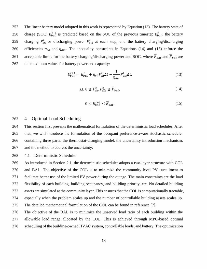
3 Models for Controllable Devices 188
3.1 HVAC Models 189
This study assumes that heating and cooling is provided by heat pumps and the heat pump energy 190
consumption represents the HVAC system energy consumption. We adopted linear regression 191
models for the HVAC system to predict room temperatures at each timestep. To precisely model 192
the building thermal reactions, two types of parameters that contribute to the heat gain of the 193
building space are considered. The first type is environmental parameters such as the outdoor air 194
dry-bulb temperature and solar irradiance. The second type represents the internal heat gain due to 195
the presence of the occupants and the operation of appliances. We assumed that the simulated 196
buildings are well sealed and thus the interference from the infiltration can be omitted. Therefore, 197
the HVAC model updates the indoor room temperature based on the room temperature at the last 198
10
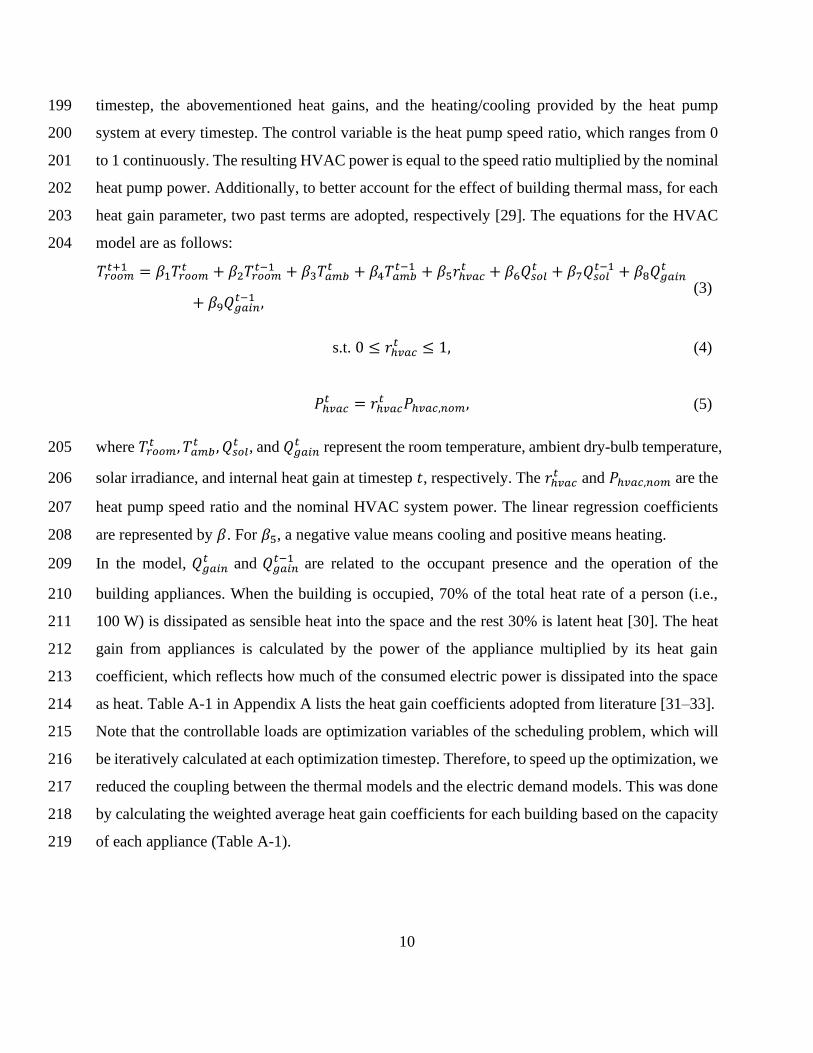
timestep, the abovementioned heat gains, and the heating/cooling provided by the heat pump 199
system at every timestep. The control variable is the heat pump speed ratio, which ranges from 0 200
to 1 continuously. The resulting HVAC power is equal to the speed ratio multiplied by the nominal 201
heat pump power. Additionally, to better account for the effect of building thermal mass, for each 202
heat gain parameter, two past terms are adopted, respectively [29]. The equations for the HVAC 203
model are as follows: 204
𝑇𝑟𝑜𝑜𝑚𝑡+1 = 𝛽1𝑇𝑟𝑜𝑜𝑚
𝑡 + 𝛽2𝑇𝑟𝑜𝑜𝑚𝑡−1 + 𝛽3𝑇𝑎𝑚𝑏
𝑡 + 𝛽4𝑇𝑎𝑚𝑏𝑡−1 + 𝛽5𝑟ℎ𝑣𝑎𝑐
𝑡 + 𝛽6𝑄𝑠𝑜𝑙𝑡 + 𝛽7𝑄𝑠𝑜𝑙
𝑡−1 + 𝛽8𝑄𝑔𝑎𝑖𝑛𝑡
+ 𝛽9𝑄𝑔𝑎𝑖𝑛𝑡−1 ,
(3)
s.t. 0 ≤ 𝑟ℎ𝑣𝑎𝑐𝑡 ≤ 1, (4)
𝑃ℎ𝑣𝑎𝑐𝑡 = 𝑟ℎ𝑣𝑎𝑐
𝑡 𝑃ℎ𝑣𝑎𝑐,𝑛𝑜𝑚, (5)
where 𝑇𝑟𝑜𝑜𝑚𝑡 , 𝑇𝑎𝑚𝑏
𝑡 , 𝑄𝑠𝑜𝑙𝑡 , and 𝑄𝑔𝑎𝑖𝑛
𝑡 represent the room temperature, ambient dry-bulb temperature, 205
solar irradiance, and internal heat gain at timestep 𝑡, respectively. The 𝑟ℎ𝑣𝑎𝑐𝑡 and 𝑃ℎ𝑣𝑎𝑐,𝑛𝑜𝑚 are the 206
heat pump speed ratio and the nominal HVAC system power. The linear regression coefficients 207
are represented by 𝛽. For 𝛽5, a negative value means cooling and positive means heating. 208
In the model, 𝑄𝑔𝑎𝑖𝑛𝑡 and 𝑄𝑔𝑎𝑖𝑛
𝑡−1 are related to the occupant presence and the operation of the 209
building appliances. When the building is occupied, 70% of the total heat rate of a person (i.e., 210
100 W) is dissipated as sensible heat into the space and the rest 30% is latent heat [30]. The heat 211
gain from appliances is calculated by the power of the appliance multiplied by its heat gain 212
coefficient, which reflects how much of the consumed electric power is dissipated into the space 213
as heat. Table A-1 in Appendix A lists the heat gain coefficients adopted from literature [31–33]. 214
Note that the controllable loads are optimization variables of the scheduling problem, which will 215
be iteratively calculated at each optimization timestep. Therefore, to speed up the optimization, we 216
reduced the coupling between the thermal models and the electric demand models. This was done 217
by calculating the weighted average heat gain coefficients for each building based on the capacity 218
of each appliance (Table A-1). 219

11
3.2 Load and Battery Models 220
The building load models in this work are categorized into four types according to their power 221
flexibility characteristics: sheddable, modulatable, shiftable, and critical (Figure 3). We did the 222
categorization from the perspective of the building owners during power outages. The sheddable 223
loads are those that can be disconnected without affecting the occupants’ essential needs. For 224
instance, the microwave in a bakery is categorized as sheddable during an outage. The modulatable 225
loads are the systems that have varying power shapes such as an HVAC system with a variable 226
frequency drive. The shiftable loads are the appliances that have flexible operation schedules such 227
as washers and dryers. Lastly, the critical loads refer to appliances and systems related to the 228
occupants’ essential needs. In this work, we consider only loads used for lighting and food 229
preservation as critical loads, which aligns with the two bottom levels of Maslow’s Hierarchy of 230
Needs (i.e., physiological and safety needs) [34]. The critical loads account for about 20% to 90% 231
of the total building loads depending on building type and time of day. 232
233
Figure 3 Power flexibility characteristics of the four load types [35]. 234
The mathematical formulation of the sheddable load is shown in Equation (6): 235
𝑃𝑠ℎ𝑒𝑑,𝑗𝑡 = 𝑢𝑠ℎ𝑒𝑑,𝑗
𝑡 �̂�𝑠ℎ𝑒𝑑,𝑗𝑡 , 𝑗 ∈ {1, … , 𝑁𝑠ℎ𝑒𝑑}, (6)
where 𝑢𝑠ℎ𝑒𝑑,𝑗𝑡 is a binary optimization variable, �̂�𝑠ℎ𝑒𝑑,𝑗
𝑡 is the original sheddable load time series 236
data, and 𝑁𝑠ℎ𝑒𝑑 is the number of sheddable loads in the building. The actual sheddable load after 237
optimization 𝑃𝑠ℎ𝑒𝑑,𝑗𝑡 is determined by the ON/OFF status represented by the binary variable. The 238
modulatable load 𝑃𝑚𝑜𝑑𝑢,𝑗𝑡 is formulated as a continuous optimization variable, which ranges 239
between zero and its original power demand �̂�𝑚𝑜𝑑𝑢,𝑗𝑡 . Equation (7) sets the lower and upper bound 240
of the modulatable load. 241
0 ≤ 𝑃𝑚𝑜𝑑𝑢,𝑗𝑡 ≤ �̂�𝑚𝑜𝑑𝑢,𝑗
𝑡 , 𝑗 ∈ {1, … , 𝑁𝑚𝑜𝑑𝑢}. (7)

12
The shiftable loads are scheduled through scheduling matrices [36]. First, using the power data 242
[37], we extracted the average cycle time 𝑛𝑠ℎ𝑖𝑓,𝑗 and the average power demand 𝑃𝑠ℎ𝑖𝑓,𝑗,𝑎𝑣𝑔 of each 243
shiftable load. The starting operation timestep 𝑡𝑠ℎ𝑖𝑓,𝑗,𝑠 of each shiftable load is optimized over the 244
MPC horizon. At the scheduled starting timestep, the binary variable 𝑣𝑠ℎ𝑒𝑑,𝑗𝑡 equals 1 and is 0 245
otherwise: 246
𝑣𝑠ℎ𝑖𝑓,𝑗𝑡 = {
1, 𝑡 = 𝑡𝑠ℎ𝑖𝑓,𝑗,𝑠,
0, 𝑡 ≠ 𝑡𝑠ℎ𝑖𝑓,𝑗,𝑠,
∀𝑡 ∈ {1, … , 𝐻 − 𝑛𝑠ℎ𝑖𝑓,𝑗 + 1}, 𝑗 ∈ {1, … , 𝑁𝑠ℎ𝑖𝑓}.
(8)
𝐻 is the MPC prediction horizon. Once the starting time of a shiftable load is selected, the power 247
demand of the load is then fixed at its average power until it finishes its cycle. The appliance must 248
finish its cycle before the horizon ends (𝑡 ∈ {1, … , 𝐻 − 𝑛𝑠ℎ𝑖𝑓,𝑗 + 1}). Here, we assume that each 249
shiftable load operates once and only once during each horizon, which is enforced by: 250
∑ 𝑣𝑠ℎ𝑖𝑓,𝑗𝑡
𝐻−𝑛𝑠ℎ𝑖𝑓,𝑗+1
𝑡=1
= 1. (9)
Next, a scheduling matrix 𝑺𝑠ℎ𝑖𝑓,𝑗 of shape 𝐻 × (𝐻 − 𝑛𝑠ℎ𝑖𝑓,𝑗 + 1) is generated for each shiftable 251
load. The actual power shape of the load, denoted 𝑃𝑠ℎ𝑖𝑓,𝑗𝑡 , is thus calculated by: 252
𝑃𝑠ℎ𝑖𝑓,𝑗𝑡 = 𝑺𝑠ℎ𝑖𝑓,𝑗 × [
𝑣𝑠ℎ𝑖𝑓,𝑗1
⋮
𝑣𝑠ℎ𝑖𝑓,𝑗
𝐻−𝑛𝑠ℎ𝑖𝑓,𝑗+1] × 𝑃𝑠ℎ𝑖𝑓,𝑗,𝑎𝑣𝑔. (10)
Finally, the actual critical load 𝑃𝑐𝑟𝑖𝑡,𝑗𝑡 must be exactly equal to the critical power demand �̂�𝑐𝑟𝑖𝑡,𝑗
𝑡 , 253
as enforced by: 254
𝑃𝑐𝑟𝑖𝑡,𝑗𝑡 = �̂�𝑐𝑟𝑖𝑡,𝑗
𝑡 , 𝑗 ∈ {1, … , 𝑁𝑐𝑟𝑖𝑡}. (11)
Summing up the four types of loads in each building, we obtain the optimization variable 𝑃𝑙𝑜𝑎𝑑𝑡 as 255
follows: 256
𝑃𝑙𝑜𝑎𝑑𝑡 = ∑ 𝑃𝑠ℎ𝑒𝑑,𝑗
𝑡
𝑁𝑠ℎ𝑒𝑑
𝑗=1
+ ∑ 𝑃𝑚𝑜𝑑𝑢,𝑗𝑡
𝑁𝑚𝑜𝑑𝑢
𝑗=1
+ ∑ 𝑃𝑠ℎ𝑖𝑓,𝑗𝑡
𝑁𝑠ℎ𝑖𝑓
𝑗=1
+ ∑ 𝑃𝑐𝑟𝑖𝑡,𝑗𝑡
𝑁𝑐𝑟𝑖𝑡
𝑗=1
. (12)
13
The linear battery model adopted in this work is represented by Equation (13). The battery state of 257
charge (SOC) 𝐸𝑏𝑎𝑡𝑡+1 is predicted based on the SOC of the previous timestep 𝐸𝑏𝑎𝑡
𝑡 , the battery 258
charging 𝑃𝑐ℎ𝑡 or discharging power 𝑃𝑑𝑖𝑠
𝑡 at each step, and the battery charging/discharging 259
efficiencies 𝜂𝑐ℎ and 𝜂𝑑𝑖𝑠 . The inequality constraints in Equations (14) and (15) enforce the 260
acceptable limits for the battery charging/discharging power and SOC, where 𝑃𝑏𝑎𝑡 and 𝐸𝑏𝑎𝑡 are 261
the maximum values for battery power and capacity: 262
𝐸𝑏𝑎𝑡𝑡+1 = 𝐸𝑏𝑎𝑡
𝑡 + 𝜂𝑐ℎ𝑃𝑐ℎ𝑡 ∆𝑡 −
1
𝜂𝑑𝑖𝑠𝑃𝑑𝑖𝑠
𝑡 ∆𝑡, (13)
s.t. 0 ≤ 𝑃𝑐ℎ𝑡 , 𝑃𝑑𝑖𝑠
𝑡 ≤ 𝑃𝑏𝑎𝑡, (14)
0 ≤ 𝐸𝑏𝑎𝑡𝑡+1 ≤ 𝐸𝑏𝑎𝑡. (15)
4 Optimal Load Scheduling 263
This section first presents the mathematical formulation of the deterministic load scheduler. After 264
that, we will introduce the formulation of the occupant preference-aware stochastic scheduler 265
containing three parts: the thermostat-changing model, the uncertainty introduction mechanism, 266
and the method to address the uncertainty. 267
4.1 Deterministic Scheduler 268
As introduced in Section 2.1, the deterministic scheduler adopts a two-layer structure with COL 269
and BAL. The objective of the COL is to minimize the community-level PV curtailment to 270
facilitate better use of the limited PV power during the outage. The main constraints are the load 271
flexibility of each building, building occupancy, and building priority, etc. No detailed building 272
assets are simulated at the community layer. This ensures that the COL is computationally tractable, 273
especially when the problem scales up and the number of controllable building assets scales up. 274
The detailed mathematical formulation of the COL can be found in reference [7]. 275
The objective of the BAL is to minimize the unserved load ratio of each building within the 276
allowable load range allocated by the COL. This is achieved through MPC-based optimal 277
scheduling of the building-owned HVAC system, controllable loads, and battery. The optimization 278

14
is a mixed-integer linear programming problem, because the sheddable and shiftable load models 279
contain binary variables. Next, the mathematical formulation of the optimization problem is 280
presented. Note that the formulation applies for every individual building in the community. 281
The cost function to minimize the unserved load ratio is formulated as: 282
𝑓𝑐𝑜𝑠𝑡(𝑡, {𝑥𝑡}𝑡=1𝐻 ) = ∑ (𝑃𝑙𝑜𝑎𝑑
𝑡− 𝑃𝑙𝑜𝑎𝑑
𝑡 )
𝐻
𝑡=1
+ ∑ 𝛾𝑃𝑐ℎ𝑡
𝐻
𝑡=1
+ ∑ 𝛾′𝑃𝑐𝑢𝑟𝑡𝑡
𝐻
𝑡=1
, (16)
𝑚𝑖𝑛{𝑥𝑡}𝑡=1
𝐻𝑓𝑐𝑜𝑠𝑡(𝑡, {𝑥𝑡}𝑡=1
𝐻 ) , (17)
where 𝑃𝑙𝑜𝑎𝑑
𝑡 is the predicted load upper bound from data. The difference between this upper bound 283
and the actual operated loads 𝑃𝑙𝑜𝑎𝑑𝑡 is minimized to achieve a maximum served load to the building. 284
To avoid simultaneous battery charging and discharging as well as PV curtailment, the objective 285
function also includes small penalizations of charging 𝛾𝑃𝑐ℎ𝑡 and curtailment 𝛾′𝑃𝑐𝑢𝑟𝑡
𝑡 [38], where 𝛾 286
and 𝛾′ are the penalization coefficients. The power balance of each building that must be satisfied 287
at each timestep is given by: 288
𝑃𝑝𝑣𝑡 − 𝑃𝑐𝑢𝑟𝑡
𝑡 = 𝑃𝑐ℎ𝑡 − 𝑃𝑑𝑖𝑠
𝑡 + 𝑃𝑙𝑜𝑎𝑑𝑡 + 𝑃ℎ𝑣𝑎𝑐
𝑡 , (18)
where PV curtailment 𝑃𝑐𝑢𝑟𝑡𝑡 is limited by how much PV generation 𝑃𝑝𝑣
𝑡 is available: 289
0 ≤ 𝑃𝑐𝑢𝑟𝑡𝑡 ≤ 𝑃𝑝𝑣
𝑡 . (19)
The left-hand side of Equation (18) represents power generation, whereas the right-hand side 290
represents consumption. The 𝑃𝑐ℎ𝑡 and 𝑃𝑑𝑖𝑠
𝑡 stand for the battery charging and discharging power as 291
in Equation (13). The 𝑃𝑙𝑜𝑎𝑑𝑡 and 𝑃ℎ𝑣𝑎𝑐
𝑡 are the total building loads and the HVAC power calculated 292
in Equations (12) and (5), respectively. To assure thermal comfort of the indoor environment, a 293
temperature constraint is given by: 294
𝑇𝑟𝑜𝑜𝑚 ≤ 𝑇𝑟𝑜𝑜𝑚𝑡 ≤ 𝑇𝑟𝑜𝑜𝑚, (20)
where 𝑇𝑟𝑜𝑜𝑚 and 𝑇𝑟𝑜𝑜𝑚 are the lower and upper room temperature bounds implemented as hard 295
constraints. The optimization variables in each building agent are collected in vector 𝑥𝑡: 296

15
𝑥𝑡 = [{𝑃𝑐𝑢𝑟𝑡
𝑡 }𝑡=1𝐻 , {𝑃𝑐ℎ
𝑡 }𝑡=1𝐻 , {𝑃𝑑𝑖𝑠
𝑡 }𝑡=1𝐻 , {𝑟ℎ𝑣𝑎𝑐
𝑡 }𝑡=1𝐻 , {𝑢𝑠ℎ𝑒𝑑,𝑗
𝑡 }𝑡=1
𝐻,
{𝑃𝑚𝑜𝑑𝑢,𝑗𝑡 }
𝑡=1
𝐻, {𝑣𝑠ℎ𝑖𝑓,𝑗
𝑡 }𝑡=1
𝐻−𝑛𝑠ℎ𝑖𝑓,𝑗+1, {𝑇𝑟𝑜𝑜𝑚
𝑡 }𝑡=1𝐻 , {𝐸𝑏𝑎𝑡
𝑡 } 𝑡=1𝐻
]. (21)
4.2 Stochastic Preference-aware Scheduler 297
To address the uncertainties of occupant thermal preference in the scheduling problem of resilient 298
communities, this section introduces the stochastic preference-aware scheduler. First, we discuss 299
the modeling of the occupant behavior uncertainties as a probability function. Then we show the 300
mechanism by which this uncertainty might affect the optimal control of the HVAC system. After 301
that, we propose using the chance-constraint method to address the uncertainty. 302
4.2.1 Stochastic Thermostat-Changing Model 303
The stochastic occupant thermostat-changing model adopted in this paper was proposed by Gunay 304
et al. [39]. Through continuous observation of the occupants’ thermostat keypress actions in 305
private office spaces, the relationship between the thermostat-changing behavior and the 306
concurrent occupancy, temperature, and relative humidity was analyzed. It was noted that the 307
frequency of thermostat interactions (i.e., increasing or decreasing) can be approximated as a 308
univariate logistic regression model with the indoor temperature as the independent predictor 309
variable. Though the original data set was obtained from two office buildings, Gunay et al. 310
generalized the study to understand occupants’ thermostat user behavior and temperature 311
preferences. Given the universality of their work, we have adapted their models based on our use 312
cases. Note that occupants might have varied (e.g., higher) tolerance of indoor temperature during 313
an emergency situation. The exact thresholds need further experimental study and validation, 314
which is out of the scope of this work. 315
The thermostat-changing behavior models determine whether the occupants will change the 316
setpoint temperature based on the concurrent indoor air temperature. The probability of increasing 317
and decreasing the temperature setpoint is predicted with a logistic regression model: 318
𝑝 =1
1 + 𝑒−(𝑎+𝑏𝑇𝑟𝑜𝑜𝑚), (22)
where 𝑝 is the probability of the changing action, 𝑇𝑟𝑜𝑜𝑚 is the indoor room temperature, and 𝑎 and 319
𝑏 are coefficients. To investigate different uncertainty levels, we proposed three different active 320

16
levels by revising the coefficients of the model in Equation (22). As shown in Table 1, the low 321
active level adopts the original coefficients in [39]. Then, we proposed the medium and high active 322
levels to represent various occupant thermal preference styles. The standard errors and p-values of 323
the low active level coefficients are also provided in the table. As for the medium and high levels, 324
we do not have measurement data for the statistical analysis since we adapted the coefficients from 325
the original reference [39]. 326
Table 1 Coefficients in different active levels of the occupant thermostat-changing behavior 327
model. 328
Active Level
Coefficients
Increasing Decreasing
a b a b
Low [39] -0.179 -0.285 -17.467 0.496
Medium 7.821 -0.485 -20.667 0.696
High 15.821 -0.685 -23.867 0.896
Standard Error 1.047 0.048 0.684 0.028
p-value 0.864 0.000 0.000 0.000
329
Note that the adaptation of the original logistic regression models was made under the following 330
assumptions to ensure the adapted models remained realistic. For the setpoint increasing scenario, 331
the slope coefficient of 𝑏 is varied linearly to reflect a higher frequency of the changing behavior. 332
The intercept coefficient 𝑎 is then calculated to make sure that all active levels have the same value 333
of probability at the temperature of 40ºC. For the setpoint decreasing scenario, a similar approach 334
is taken to make sure the same value of probability at 16ºC is shared by all active levels. At each 335
thermostat interaction, we assume that 1ºC of setpoint change would take place. Figure 4 depicts 336
the probabilities of the three active levels. Note that this figure contains a wider temperature range 337
than 16ºC ~ 40ºC to show a more comprehensive performance of the behavior models. 338
339

17
340
Figure 4 Probability of different thermostat-changing behavior. 341
Once the probability of the thermostat-changing behavior is determined using the above models, 342
the increasing or decreasing action is determined by comparing the probabilities with a randomly 343
generated number. At each optimization timestep, a random number between 0 and 1 is generated. 344
If the number is larger than 1 − Pr (𝑖𝑛𝑐𝑟𝑒𝑎𝑠𝑒), the action will be to increase. On the contrary, if 345
it is smaller than Pr (𝑑𝑒𝑐𝑟𝑒𝑎𝑠𝑒), the action will be to decrease. Because the sum of the increase 346
and decrease probabilities is smaller than 1 in our case, this algorithm assures at most one action 347
will be taken at each timestep. 348
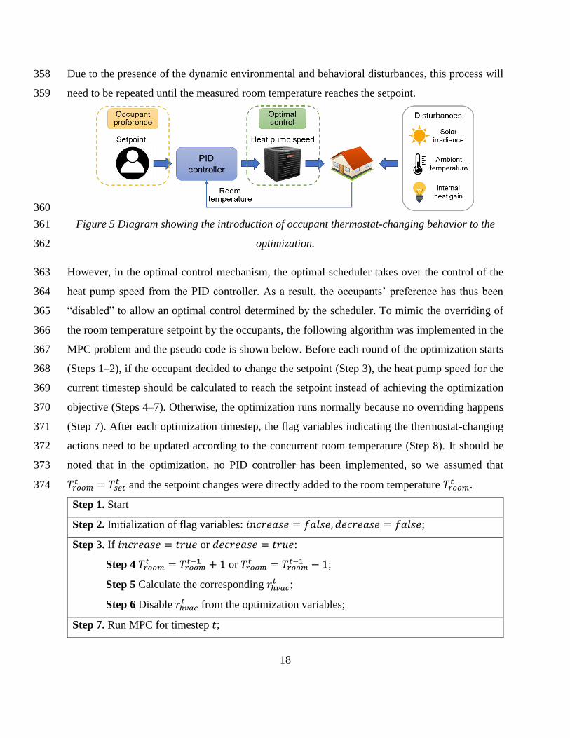
4.2.2 Introducing Occupant Behavior Uncertainties in Scheduling 349
To introduce the occupant thermostat-changing uncertainties to the load scheduling problem, a 350
stochastic simulation model representing the behavior needs to be incorporated into the 351
optimization. Figure 5 shows the control signal flow for the typical indoor air temperature control, 352
which affects the HVAC system operational status and its power consumption. The occupant sets 353
the temperature setpoint according to his/her preference through the thermostat. Behind the 354
thermostat, a proportional integral derivative (PID) controller decides the next heat pump speed to 355
offset the difference between the measured room temperature and the setpoint. This heat pump 356
speed signal is then fed into the heat pump system to provide cooling for the conditioned space. 357
18
Due to the presence of the dynamic environmental and behavioral disturbances, this process will 358
need to be repeated until the measured room temperature reaches the setpoint. 359
360
Figure 5 Diagram showing the introduction of occupant thermostat-changing behavior to the 361
optimization. 362
However, in the optimal control mechanism, the optimal scheduler takes over the control of the 363
heat pump speed from the PID controller. As a result, the occupants’ preference has thus been 364
“disabled” to allow an optimal control determined by the scheduler. To mimic the overriding of 365
the room temperature setpoint by the occupants, the following algorithm was implemented in the 366
MPC problem and the pseudo code is shown below. Before each round of the optimization starts 367
(Steps 1–2), if the occupant decided to change the setpoint (Step 3), the heat pump speed for the 368
current timestep should be calculated to reach the setpoint instead of achieving the optimization 369
objective (Steps 4–7). Otherwise, the optimization runs normally because no overriding happens 370
(Step 7). After each optimization timestep, the flag variables indicating the thermostat-changing 371
actions need to be updated according to the concurrent room temperature (Step 8). It should be 372
noted that in the optimization, no PID controller has been implemented, so we assumed that 373
𝑇𝑟𝑜𝑜𝑚𝑡 = 𝑇𝑠𝑒𝑡
𝑡 and the setpoint changes were directly added to the room temperature 𝑇𝑟𝑜𝑜𝑚𝑡 . 374
Step 1. Start
Step 2. Initialization of flag variables: 𝑖𝑛𝑐𝑟𝑒𝑎𝑠𝑒 = 𝑓𝑎𝑙𝑠𝑒, 𝑑𝑒𝑐𝑟𝑒𝑎𝑠𝑒 = 𝑓𝑎𝑙𝑠𝑒;
Step 3. If 𝑖𝑛𝑐𝑟𝑒𝑎𝑠𝑒 = 𝑡𝑟𝑢𝑒 or 𝑑𝑒𝑐𝑟𝑒𝑎𝑠𝑒 = 𝑡𝑟𝑢𝑒:
Step 4 𝑇𝑟𝑜𝑜𝑚𝑡 = 𝑇𝑟𝑜𝑜𝑚
𝑡−1 + 1 or 𝑇𝑟𝑜𝑜𝑚𝑡 = 𝑇𝑟𝑜𝑜𝑚
𝑡−1 − 1;
Step 5 Calculate the corresponding 𝑟ℎ𝑣𝑎𝑐𝑡 ;
Step 6 Disable 𝑟ℎ𝑣𝑎𝑐𝑡 from the optimization variables;
Step 7. Run MPC for timestep 𝑡;

19
Step 8. Update flag variables (i.e., 𝑖𝑛𝑐𝑟𝑒𝑎𝑠𝑒 and 𝑑𝑒𝑐𝑟𝑒𝑎𝑠𝑒) according to 𝑇𝑟𝑜𝑜𝑚𝑡 ;
Step 9. Repeat Steps 3–8 until the end of the MPC horizon of 48 hours;
Step 10. End
4.2.3 Chance-Constraint Method 375
As mentioned in Section 4.2.1, the uncertainties in the occupants’ thermostat-changing behavior 376
are a probability function. In the scheduling optimization problem, the constraint directly affected 377
by the occupants’ thermostat-changing behavior is the room temperature bounds. The uncertainties 378
related to the occupants’ adjusting the thermostat could lead to the violation of the temperature 379
bounds during the implementation of the developed control strategies. Furthermore, this could lead 380
to other control-related performances being affected, including higher building load unserved ratio 381
and larger required battery size. To address this, we adopted the chance-constraint method. 382
By definition, the chance constraint allows the violation of a certain constraint with a small 383
probability, which thus presents a systematic trade-off between control performance and 384
probability of constraint violations [40]. It can be expressed in general by the following equation: 385
𝑃𝑟(𝑔(𝑥, 𝜉) ≤ 0) ≥ 1 − 𝜖, (23)
where 𝑔(𝑥, 𝜉) ≤ 0 is the inequivalent constraint and 𝜖 is the maximum violation probability. 386
Given the uncertainties in the occupants’ thermostat-changing behavior, we assume that the 387
temperature bounds can be satisfied with a probability of (1 − 𝜖𝑇). For the lower temperature 388
bounds, the chance constraint can thus be written as: 389
𝑃𝑟(𝑇𝑟𝑜𝑜𝑚 ≤ 𝑇𝑟𝑜𝑜𝑚𝑡+1 ) ≥ 1 − 𝜖𝑇 . (24)
Then, we rewrite it as: 390
𝑃𝑟(𝜒𝑇𝑡+1 ≤ 0) ≥ 1 − 𝜖𝑇 , (25)
where 𝜒𝑇𝑡+1 = 𝑇𝑟𝑜𝑜𝑚 − 𝑇𝑟𝑜𝑜𝑚
𝑡+1 . Let the indoor temperature be rewritten in terms of the prediction 391
error: 𝑇𝑟𝑜𝑜𝑚𝑡 = 𝑇𝑟𝑜𝑜𝑚,𝑓
𝑡 + 𝑇𝑟𝑜𝑜𝑚,𝑒𝑡 where 𝑇𝑟𝑜𝑜𝑚,𝑓
𝑡 is the predicted indoor room temperature and 392
𝑇𝑟𝑜𝑜𝑚,𝑒𝑡 is the error caused by uncertainties. Similarly, 𝑇𝑟𝑜𝑜𝑚
𝑡−1 = 𝑇𝑟𝑜𝑜𝑚,𝑓𝑡−1 + 𝑇𝑟𝑜𝑜𝑚,𝑒
𝑡−1 . For both 393
timesteps, the room temperature distribution error follows the same distribution. The hypothetical 394
20
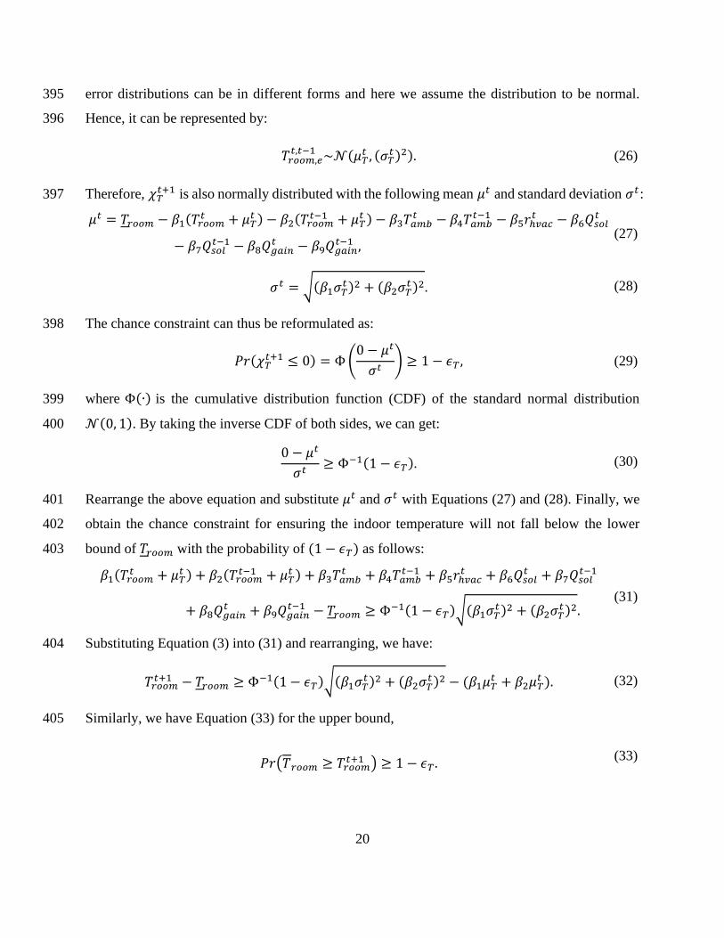
error distributions can be in different forms and here we assume the distribution to be normal. 395
Hence, it can be represented by: 396
𝑇𝑟𝑜𝑜𝑚,𝑒𝑡,𝑡−1 ~𝒩(𝜇𝑇
𝑡 , (𝜎𝑇𝑡 )2). (26)
Therefore, 𝜒𝑇𝑡+1 is also normally distributed with the following mean 𝜇𝑡 and standard deviation 𝜎𝑡: 397
𝜇𝑡 = 𝑇𝑟𝑜𝑜𝑚 − 𝛽1(𝑇𝑟𝑜𝑜𝑚𝑡 + 𝜇𝑇
𝑡 ) − 𝛽2(𝑇𝑟𝑜𝑜𝑚𝑡−1 + 𝜇𝑇
𝑡 ) − 𝛽3𝑇𝑎𝑚𝑏𝑡 − 𝛽4𝑇𝑎𝑚𝑏
𝑡−1 − 𝛽5𝑟ℎ𝑣𝑎𝑐𝑡 − 𝛽6𝑄𝑠𝑜𝑙
𝑡
− 𝛽7𝑄𝑠𝑜𝑙𝑡−1 − 𝛽8𝑄𝑔𝑎𝑖𝑛
𝑡 − 𝛽9𝑄𝑔𝑎𝑖𝑛𝑡−1 ,
(27)
𝜎𝑡 = √(𝛽1𝜎𝑇𝑡 )2 + (𝛽2𝜎𝑇
𝑡 )2. (28)
The chance constraint can thus be reformulated as: 398
𝑃𝑟(𝜒𝑇𝑡+1 ≤ 0) = Φ (
0 − 𝜇𝑡
𝜎𝑡) ≥ 1 − 𝜖𝑇 , (29)
where Φ(∙) is the cumulative distribution function (CDF) of the standard normal distribution 399
𝒩(0, 1). By taking the inverse CDF of both sides, we can get: 400
0 − 𝜇𝑡
𝜎𝑡≥ Φ−1(1 − 𝜖𝑇). (30)
Rearrange the above equation and substitute 𝜇𝑡 and 𝜎𝑡 with Equations (27) and (28). Finally, we 401
obtain the chance constraint for ensuring the indoor temperature will not fall below the lower 402
bound of 𝑇𝑟𝑜𝑜𝑚 with the probability of (1 − 𝜖𝑇) as follows: 403
𝛽1(𝑇𝑟𝑜𝑜𝑚𝑡 + 𝜇𝑇
𝑡 ) + 𝛽2(𝑇𝑟𝑜𝑜𝑚𝑡−1 + 𝜇𝑇
𝑡 ) + 𝛽3𝑇𝑎𝑚𝑏𝑡 + 𝛽4𝑇𝑎𝑚𝑏
𝑡−1 + 𝛽5𝑟ℎ𝑣𝑎𝑐𝑡 + 𝛽6𝑄𝑠𝑜𝑙
𝑡 + 𝛽7𝑄𝑠𝑜𝑙𝑡−1
+ 𝛽8𝑄𝑔𝑎𝑖𝑛𝑡 + 𝛽9𝑄𝑔𝑎𝑖𝑛
𝑡−1 − 𝑇𝑟𝑜𝑜𝑚 ≥ Φ−1(1 − 𝜖𝑇)√(𝛽1𝜎𝑇𝑡 )2 + (𝛽2𝜎𝑇
𝑡 )2. (31)
Substituting Equation (3) into (31) and rearranging, we have: 404
𝑇𝑟𝑜𝑜𝑚𝑡+1 − 𝑇𝑟𝑜𝑜𝑚 ≥ Φ−1(1 − 𝜖𝑇)√(𝛽1𝜎𝑇
𝑡 )2 + (𝛽2𝜎𝑇𝑡 )2 − (𝛽1𝜇𝑇
𝑡 + 𝛽2𝜇𝑇𝑡 ). (32)
Similarly, we have Equation (33) for the upper bound, 405
𝑃𝑟(𝑇𝑟𝑜𝑜𝑚 ≥ 𝑇𝑟𝑜𝑜𝑚𝑡+1 ) ≥ 1 − 𝜖𝑇 .
(33)

21
Taking a similar derivation process as that in Equations (24) to (32), we can obtain the chance 406
constraint for the temperature upper bound: 407
𝑇𝑟𝑜𝑜𝑚 − 𝑇𝑟𝑜𝑜𝑚𝑡+1 ≥ Φ−1(1 − 𝜖𝑇)√(𝛽1𝜎𝑇
𝑡 )2 + (𝛽2𝜎𝑇𝑡 )2 + (𝛽1𝜇𝑇
𝑡 + 𝛽2𝜇𝑇𝑡 ). (34)
The updated inequivalent constraints indicate that the temperature bounds for the optimization 408
should be narrower than the original temperature bounds to account for the setpoint behavioral 409
uncertainty, which is consistent with the expectations. Note that because the uncertainty-dealing 410
method is focused on the temperature constraints, one possible limitation is that the above method 411
might have limited effect on the controller design for buildings that have larger thermal masses, 412
because the building temperature is insensitive to temperature constraints. More discussion of this 413
point follows in Section 5.3.1. 414
5 Case Study 415
5.1 Studied Community 416
The case study community is a net-zero energy community located in Anna Maria Island, Florida, 417
USA, which is a cooling dominated region. The community buildings are installed with both roof-418
top PV panels and solar carports, which harvest about 85 MWh annually for the whole community. 419
A centralized ground source heat pump system provides the HVAC needs of the whole community 420
with high efficiency. Other sustainable features include well-insulated building envelopes, solar 421
thermal water heating, and rainwater recycling. This community achieved net-zero energy in the 422
year of 2014. In the community, there are various building types such as residential, small office, 423
gift shop, etc. We would like to cover both residential and commercial buildings in the case study. 424
So, we selected one residential and two small commercial buildings based on the measurement 425
data quality. More specifically, the selected three buildings consist of a residential building (area: 426
93.8 m2), an ice cream shop (area: 160.5 m2), and a bakery (area: 410 m2). The building layout of 427
the community can be found in reference [28]. 428
For the given community, a virtual testbed based on the object-oriented modeling language 429
Modelica [41] was built and validated [42]. In the testbed, the Typical Meteorological Year 3 data 430
for a nearby city, Tampa, was adopted for this case study. The building thermal models are 431
resistance-capacitance (RC) network models. For the optimal control in this work, the HVAC 432

22
models were trained using one month (i.e., August) of the simulation data exported from the 433
testbed. Table 2 lists the coefficients for the linear regression HVAC models, the Root Mean 434
Square Error (RMSE) of the models, as well as the corresponding nominal heat pump power. The 435
N/A in the table represents a coefficient that is too small and thus has been neglected in the model. 436
Three effective decimal places are provided. 437
Table 2 Coefficients and nominal power of the HVAC models. 438
Residential Ice Cream
Shop Bakery
Coefficients
𝑇𝑟𝑜𝑜𝑚𝑡 1.429 0.502 0.977
𝑇𝑟𝑜𝑜𝑚𝑡−1 -0.432 0.498 0.0213
𝑇𝑎𝑚𝑏𝑡 0.0263 0.000295 0.00405
𝑇𝑎𝑚𝑏𝑡−1 -0.0232 -0.000193 -0.00196
𝑟ℎ𝑣𝑎𝑐𝑡 -0.210 -0.0114 -0.178
𝑄𝑠𝑜𝑙𝑡 0.0151 0.0000345 0.0107
𝑄𝑠𝑜𝑙𝑡−1 -0.00302 0.000181 -0.00621
𝑄𝑔𝑎𝑖𝑛𝑡 0.00852 N/A N/A
𝑄𝑔𝑎𝑖𝑛𝑡−1 N/A N/A 0.0140
RMSE [℃] 0.160 0.0205 0.114
Nominal Power [kW] 2.140 2.830 3.770
439
Additionally, Table 3 lists the load categorization for the studied buildings following the principles 440
proposed in Section 3.2. A complete list of the building load capacities and their heat gains can be 441
found in Appendix A. 442
Table 3 Building loads categorized into four types. 443
Residential Ice Cream Shop Bakery
Sheddable Computer
Coffee maker, soda
dispenser, outdoor
ice storage
Microwave
Modulatable HVAC HVAC Mixer, unspecific room
plug loads, HVAC
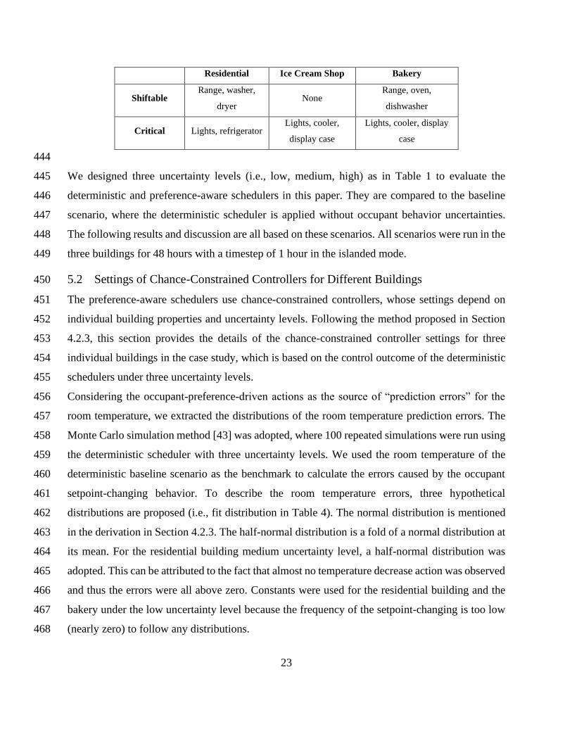
23
Residential Ice Cream Shop Bakery
Shiftable Range, washer,
dryer None
Range, oven,
dishwasher
Critical Lights, refrigerator Lights, cooler,
display case
Lights, cooler, display
case
444
We designed three uncertainty levels (i.e., low, medium, high) as in Table 1 to evaluate the 445
deterministic and preference-aware schedulers in this paper. They are compared to the baseline 446
scenario, where the deterministic scheduler is applied without occupant behavior uncertainties. 447
The following results and discussion are all based on these scenarios. All scenarios were run in the 448
three buildings for 48 hours with a timestep of 1 hour in the islanded mode. 449
5.2 Settings of Chance-Constrained Controllers for Different Buildings 450
The preference-aware schedulers use chance-constrained controllers, whose settings depend on 451
individual building properties and uncertainty levels. Following the method proposed in Section 452
4.2.3, this section provides the details of the chance-constrained controller settings for three 453
individual buildings in the case study, which is based on the control outcome of the deterministic 454
schedulers under three uncertainty levels. 455
Considering the occupant-preference-driven actions as the source of “prediction errors” for the 456
room temperature, we extracted the distributions of the room temperature prediction errors. The 457
Monte Carlo simulation method [43] was adopted, where 100 repeated simulations were run using 458
the deterministic scheduler with three uncertainty levels. We used the room temperature of the 459
deterministic baseline scenario as the benchmark to calculate the errors caused by the occupant 460
setpoint-changing behavior. To describe the room temperature errors, three hypothetical 461
distributions are proposed (i.e., fit distribution in Table 4). The normal distribution is mentioned 462
in the derivation in Section 4.2.3. The half-normal distribution is a fold of a normal distribution at 463
its mean. For the residential building medium uncertainty level, a half-normal distribution was 464
adopted. This can be attributed to the fact that almost no temperature decrease action was observed 465
and thus the errors were all above zero. Constants were used for the residential building and the 466
bakery under the low uncertainty level because the frequency of the setpoint-changing is too low 467
(nearly zero) to follow any distributions. 468

24
Chi-square goodness of fit tests [44] at a rejection level of 1% were conducted to evaluate whether 469
the proposed hypothetical distributions fit well. The types of fitting distributions, p-values of the 470
tests, and the distribution parameters are reported in Table 4. In the table, µ is the mean and σ is 471
the standard deviation of the normal/half-normal distribution. The null hypothesis here is that the 472
room temperature prediction error follows the hypothetical distribution. The p-value is the 473
evidence against this null hypothesis. Since all p-values are greater than 99%, all error distributions 474
failed to reject the hypothesis at the level of 1%. This means they all follow the corresponding 475
hypothetical distribution. 476
Table 4 Chi-square goodness of fit test p-values and normal distribution parameters. 477
Building Uncertainty Fit Distribution p-value µ [ºC] σ [ºC]
Residential
Low Constant 1.0 -6.45E-05 N/A
Medium Half-normal 0.999 -3.57E-01 4.35E-01
High Normal 0.999 1.56E+00 8.17E-01
Ice Cream Shop
Low Normal 0.999 -3.48E-03 7.86E-03
Medium Normal 0.999 -4.45E-03 8.59E-03
High Normal 0.999 1.60E-02 1.59E-02
Bakery
Low Constant 1.0 -3.42E-03 N/A
Medium Normal 0.999 3.01E-02 1.05E-01
High Normal 0.999 5.33E-01 4.65E-01
The frequency histogram and probability density functions (PDFs) of each building under various 478
uncertainty levels are plotted in Figure 6. In the figure, it can be seen that the higher the uncertainty, 479
the wider the room temperature range. This is because in scenarios with a higher uncertainty, 480
occupants change the thermostat more frequently, which expands the possible temperature ranges. 481
We also noticed that the temperature range in the ice cream shop is relatively concentrated 482
compared to the other two buildings. This can be attributed to the large thermal mass of the 483
building. 484

25
485
Figure 6 Room temperature prediction error PDFs obtained from the Monte Carlo simulations. 486
For the scenario where the temperature prediction error follows the half-normal distribution, we 487
applied the chance constraint only to the upper bound because only increasing actions happen in 488
this scenario. For the two scenarios where the room temperature error is estimated to be a constant, 489
we adopted the original temperature bounds of [20ºC, 25ºC] because the estimated errors in both 490
scenarios are smaller than 0.01ºC. We choose the 𝜖𝑇 = 1% to ensure a 99% probability of 491
abidance of the temperature constraints (Equation (24)). Table 5 lists the updated room 492
temperature lower and upper bounds for each building under different scenarios. 493
Table 5 Room temperature bounds for chance-constrained optimizations. 494
Building Uncertainty 𝑻𝒓𝒐𝒐𝒎 [ºC] 𝑻𝒓𝒐𝒐𝒎 [ºC]
Residential
Low 20.000 25.000
Medium 20.000 24.236
High 20.547 21.343
Ice Cream
Shop
Low 20.024 24.983
Medium 20.027 24.982
High 20.025 24.943
Bakery
Low 20.000 25.000
Medium 20.240 24.700
High 20.664 23.273
495

26
5.3 Results and Discussions 496
This section first quantifies the impact of introducing occupant behavior uncertainties to the 497
optimal scheduling problem. Then, the deterministic and chance-constrained controllers are tested 498
on the community virtual testbed. Their control performance in terms of the unserved load ratio, 499
the required battery size, and the unmet thermal preference hours are then compared. 500
5.3.1 Impact of Uncertainty 501
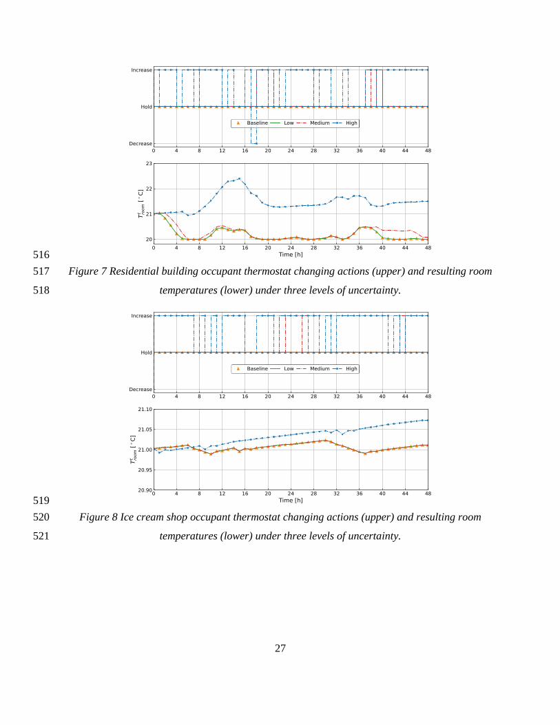
Figures 7 to 9 depict the occupant thermal preference and the corresponding room temperatures. 502
In the figures, the upper plots show the simulated stochastic thermostat-changing actions at 503
different uncertainty levels, where increase means a setpoint increase action, and vice versa. The 504
lower plots show the resulting room temperatures with dashed lines. 505
The results of the low uncertainty scenario overlap with that of the baseline scenario (i.e., the 506
deterministic scheduler without uncertainty) mainly due to the low probability of setpoint-507
changing actions in this scenario. With the increase in the probability, we see more frequent 508
setpoint-changing actions in all three buildings. Further, the increase action happens more 509
frequently than the decrease action. This is because between the temperature range of 20ºC and 510
24ºC, the probability of increase is much higher than that of decrease (see Figure 4). This also 511
implies that the occupants’ temperature preference is closer to 24ºC than 20ºC. Additionally, for 512
the residential building and the bakery, the temperature difference between scenarios is more 513
noticeable than for the ice cream shop; this is attributable to the different building thermal masses 514
of the three buildings. 515
27
516
Figure 7 Residential building occupant thermostat changing actions (upper) and resulting room 517
temperatures (lower) under three levels of uncertainty. 518
519
Figure 8 Ice cream shop occupant thermostat changing actions (upper) and resulting room 520
temperatures (lower) under three levels of uncertainty. 521

28
522
Figure 9 Bakery occupant thermostat changing actions (upper) and resulting room temperatures 523
(lower) under three levels of uncertainty. 524
Table 6 lists the values of the KRIs in correspondence with Figures 7 to 9. The HVAC energy and 525
average room temperature over the optimization horizon are also provided to facilitate the analysis 526
of the results. 527
Table 6 Key resilience indicators for studied buildings under different uncertainty levels. 528
Building Scenario Unserved Load Ratio Battery Size [kWh] HVAC Energy
[kWh]
Mean Room
Temperature [ºC]
Residential
Baseline 0.0744 47.686 32.139 20.185
Low 0.0744 47.686 32.139 20.185
Medium 0.0744 47.168 32.099 20.271
High 0.0744 38.541 21.400 21.468
Ice Cream Shop
Baseline 0.0215 99.139 32.703 21.006
Low 0.0215 99.139 32.703 21.006
Medium 0.0215 99.139 32.703 21.006
High 0.0215 93.166 10.063 21.033
Bakery
Baseline 0.0247 80.007 35.144 21.579
Low 0.0247 80.007 35.144 21.579
Medium 0.0247 73.496 27.604 21.766
High 0.0247 76.801 11.310 21.973
529

29
From the table, we see that the unserved load ratio remains the same across all scenarios for each 530
building. This can be attributed to the fact that in the controller design phase, the optimization 531
objective is set to minimize the unserved load ratio. Hence, the unserved load ratios for each 532
building are already minimal and are not affected by the occupants’ thermostat-overriding 533
behavior uncertainties. Instead, the battery-charging/discharging behavior is affected, as reflected 534
by the different required battery sizes in the table. Note that the unserved load ratios are minimal, 535
but not zero, because of our assumption that each shiftable load operates once and only once per 536
day. 537
For the rest of the metrics, note that the battery size, HVAC energy, and the average room 538
temperature remain the same for the baseline and low uncertainty scenarios in all buildings. This 539
is because no setpoint-changing actions happened due to the relatively low probabilities, as shown 540
in the figures above. As for the medium uncertainty scenarios, both the residential building and 541
the bakery show higher room temperatures and lower HVAC energy while the ice cream shop still 542
has the same results as the baseline, given its large thermal mass. 543
In terms of the high uncertainty scenarios, due to the prominent increase in room temperatures, we 544
noticed more HVAC energy savings in all buildings. Note that though the average room 545
temperature increase is insignificant, the HVAC energy savings is large due to the cumulative 546
effect over the many hours of setpoint increase. Overall, we see a positive correlation between the 547
HVAC energy and the required battery size. When the PV generation and the other building loads 548
remain the same, the more HVAC energy, the larger required battery size. However, one opposite 549
case was noted in the bakery high uncertainty scenario where the required battery size is slightly 550
larger in the high uncertainty scenario than in the medium uncertainty scenario. This was caused 551
by a setpoint decrease action at hour 28, which resulted in a battery discharging during the night 552
and thus a smaller minimum SOC of the battery. 553
To summarize, occupant thermostat-changing behavior uncertainty needs to be considered when 554
designing optimal schedulers for resilient buildings because it affects the indoor room temperature, 555
the HVAC power, and thus the sizing of batteries. For the whole community, when considering 556
the highest occupant behavior uncertainty, the consumed HVAC energy can be 57.2% less and the 557
battery 8.08% smaller. Whereas the aforementioned impact depends on the uncertainty level (i.e., 558
how frequently the occupants change the setpoint), heating or cooling season, and the occupants’ 559

30
actual preference for the indoor room temperature compared to the room temperature designed by 560
the scheduler. In our case, a preferred higher indoor room temperature saves HVAC energy. 561
During the heating season, the observations could be the reversed. 562
5.3.2 Controller Performance 563
To further evaluate the performance of the chance-constrained controller in comparison with the 564
deterministic controller, tests were run on the virtual testbed [28] in a stochastic manner. In each 565
of the studied buildings, both the deterministic controller and the chance-constrained controller 566
were tested for two days (i.e., August 4 and 5) with the three levels of uncertainties. The testing 567
method is similar to the method proposed in Section 4.2.2. Additionally, the precalculated optimal 568
battery charging/discharging, as well as the optimized loads, are also implemented in the testbed. 569
One hundred repeated Monte Carlo simulations were run for each scenario to better observe the 570
controller performance. The KRIs of the unserved load ratio, the required battery size, and the 571
unmet thermal preference hours are adopted for the performance evaluation. 572
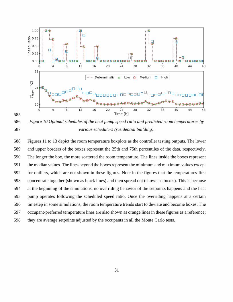
The upper plot of Figure 10 depicts the predetermined optimal schedules of the heat pump speed 573
ratio as the inputs of the test. The lower plot then shows the corresponding room temperatures 574
predicted by the linear regression models in the optimization. The data for the residential building 575
is adopted here for the analysis. The plots for the ice cream shop and the bakery can be found in 576
Appendix A. From the figure, we see that the scheduled speed ratios in the low and medium 577
uncertainty scenarios overlap with that of the deterministic scheduler. Whereas the high 578
uncertainty scenario tends to have lower speed ratios over the whole optimization horizon. This 579
can be attributed to the controller settings shown in Table 5, where the temperature bounds set in 580
the low and medium uncertainty scenarios are closer to the original bounds of [20ºC–25ºC]. Hence, 581
the temperature constraints are not binding in these two scenarios. However, in the high 582
uncertainty scenario, the temperature constraint is binding, which leads to the speed ratio 583
reductions. As a result, a higher room temperature can be seen in the high uncertainty scenario. 584
31
585
Figure 10 Optimal schedules of the heat pump speed ratio and predicted room temperatures by 586
various schedulers (residential building). 587
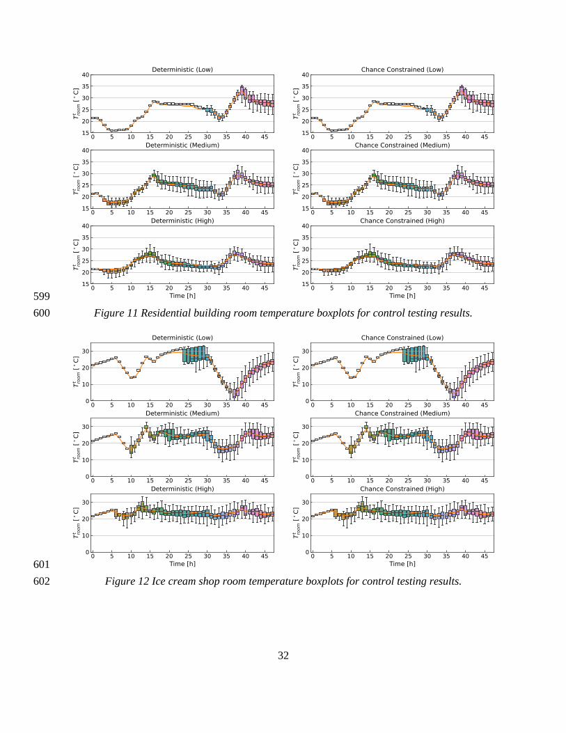
Figures 11 to 13 depict the room temperature boxplots as the controller testing outputs. The lower 588
and upper borders of the boxes represent the 25th and 75th percentiles of the data, respectively. 589
The longer the box, the more scattered the room temperature. The lines inside the boxes represent 590
the median values. The lines beyond the boxes represent the minimum and maximum values except 591
for outliers, which are not shown in these figures. Note in the figures that the temperatures first 592
concentrate together (shown as black lines) and then spread out (shown as boxes). This is because 593
at the beginning of the simulations, no overriding behavior of the setpoints happens and the heat 594
pump operates following the scheduled speed ratio. Once the overriding happens at a certain 595
timestep in some simulations, the room temperature trends start to deviate and become boxes. The 596
occupant-preferred temperature lines are also shown as orange lines in these figures as a reference; 597
they are average setpoints adjusted by the occupants in all the Monte Carlo tests. 598
32
599
Figure 11 Residential building room temperature boxplots for control testing results. 600
601
Figure 12 Ice cream shop room temperature boxplots for control testing results. 602

33
603
Figure 13 Bakery room temperature boxplots for control testing results. 604
In the figures, we see a general trend of narrower room temperature ranges from the low 605
uncertainty scenarios to high uncertainty scenarios. This is due to the introduction of the occupant 606
setpoint-overriding mechanism, which tends to moderate the extreme room temperatures. Also, 607
there is a plant-model mismatch, which describes the parametric uncertainty of modeling that 608
originates from neglected dynamics of the plant [25]. In our case, the mismatch exists as the 609
simulated room temperatures in the testbed are slightly higher than those predicted by the reduced-610
order linear HVAC models. This is understandable because the physics-based testbed has a much 611
higher fidelity and simulates the non-linearity of the real mechanical systems. 612
Because the difference in the room temperature between the two controllers is not depicted in these 613
figures, Table 7 and Table 8 provide further quantitative evaluations of the room temperatures 614
along with other controller performance. Additionally, note that the optimal schedules of some 615
scenarios remain the same because of the unbinding temperature constraints, which led to the same 616
testing outputs. Here we only discuss the scenarios that have different inputs and outputs. A full 617
list of all testing results is available in Table A-2. 618
Table 7 Comparison of controller performance in the residential building high uncertainty 619
scenario. 620

34
Controller
Unmet Thermal
Preference Hours
[ºC·h]
Mean Room
Temperature [ºC]
Unserved
Load Ratio
Required
Battery Size
[kWh]
Deterministic 48.91 23.75 0.074 47.69
Chance-
constrained 46.42 23.87 0.074 44.12
621
In Table 7, we see a larger value of unmet thermal preference hours in the deterministic controller 622
than the chance-constrained one. This can be attributed to the higher room temperatures regulated 623
by the chance constraints to better satisfy the occupants’ thermal preferences. Again, the same 624
unserved load ratio is observed in both controllers because it is already minimal, which is enforced 625
by the objective function. In terms of the battery size, the chance-constrained controller shows a 626
smaller required battery size than the deterministic controller. This results from the fact that a 627
higher room temperature has led to less consumed HVAC energy in the chance-constrained 628
scenario. Thus, less discharging from the battery was happening, which led to a smaller required 629
battery size. For the bakery results shown in Table 8, the same trends for the battery size and the 630
unserved load ratio as the residential building can be observed under each uncertainty level. 631
Namely, smaller batteries and the same unserved load ratios. 632
Table 8 Comparison of controller performances in the bakery medium and high uncertainty 633
scenarios. 634
Uncertainty Controller
Unmet Thermal
Preference
Hours [ºC·h]
Mean Room
Temperature
[ºC]
Unserved
Load Ratio
Required
Battery Size
[kWh]
Medium
Deterministic 88.80 24.27 0.025 80.01
Chance-
constrained 91.28 24.50 0.025 76.89
High
Deterministic 102.81 23.65 0.025 80.01
Chance-
constrained 101.61 23.89 0.025 76.89
635

35
As for the unmet thermal preference hours, different trends are witnessed in the medium and high 636
uncertainty levels. In the medium level, the deterministic controller shows fewer unmet preference 637
hours than the chance-constrained controller. Whereas in the high uncertainty level, an opposite 638
trend is seen. This is reasonable as we see a generally higher mean room temperature regulated by 639
the chance-constrained controller under different uncertainty levels. However, in the medium 640
scenario, a lower preference temperature line was obtained from the Monte Carlo testing, which is 641
closer to the actual room temperatures of the deterministic controller. When the preference 642
temperature rises in the high uncertainty scenario, the chance-constrained controller outperforms 643
the deterministic controller with a higher actual room temperature and thus smaller unmet thermal 644
preference hours. 645
When we compare different uncertainty levels in the bakery, we see that the mean room 646
temperature decreases with the increase in uncertainty. This is because the lower temperature 647
upper bounds shown in Table 5 have regulated the room temperature to sink when the uncertainty 648
gets higher. Additionally, as seen in Figure 4, in the temperature range of 20ºC to 24ºC, the 649
probability of increasing the temperature setpoint is much higher than that of decreasing it While 650
above 24ºC, the probability to increase and to decrease is almost the same. This has caused the 651
room temperatures to end up around 24ºC in the high uncertainty scenarios for all buildings (Table 652
A-2). This reveals that with the increase in the occupant thermostat-changing uncertainties, the 653
room temperatures tend to get closer to the occupants’ preferred room temperature. 654
Though some improvement was noticed in the chance-constrained controller compared to the 655
deterministic controller, the overall improvement was less than expected. This could be attributed 656
to the following three factors. First, the impact of the uncertainty level on the controller 657
performance improvement is prominent as we observe higher performance improvement in high 658
uncertainty scenarios. Second, the thermal property, especially thermal mass, of the building itself 659
also affects the results. Thermal mass serves as a thermal buffer to filter the impact of various 660
HVAC supply temperatures. Hence, buildings with a larger thermal mass tend to experience less 661
impact from the occupant thermal preference uncertainty. This can be demonstrated by the results 662
of the ice cream shop, where the two controllers perform the same. Third, the plant-model 663
mismatch also plays a significant role in the transition from the optimal scheduler design to its 664
implementation. In the design phase, a series of control-oriented linear regression building models 665

36
was used. However, the testing took place on a high-fidelity physics-based testbed, where the 666
complex system dynamics of the whole buildings and HVAC systems were modeled with shorter 667
simulation timesteps. This is a common source of uncertainty to be addressed for MPC design and 668
implementation. 669
In our opinion, joint effort from building scientists, modelers, and engineers is needed to facilitate 670
implementing stochasticity in the building domain and ultimately better serve the occupants. For 671
example, an open-source database focused on building performance related stochasticity such as 672
the occupant behavior and weather forecast needs to be established. Further, readily available 673
stochastic simulation tools need to be developed (e.g., Occupancy Simulator [45]). Finally, 674
stochasticity needs to be incorporated into the whole process of building modeling and design in 675
the form of boundary conditions or internal components. 676
6 Conclusion 677
In this paper, we proposed a preference-aware scheduler for resilient communities. Stochastic 678
occupant thermostat-changing behavior models were introduced into a deterministic load 679
scheduling framework as a source of uncertainty. The impact of occupant behavior uncertainty on 680
community optimal scheduling strategies was discussed. KRIs such as the unserved load ratio, the 681
required battery size, and the unmet thermal preference hours were adopted to quantify the impacts 682
of uncertainties. Generally, the proposed controller performs better in terms of the unmet thermal 683
preference hours and the battery sizes compared to the deterministic controller. Though only tested 684
on three buildings of the studied community, the methodology of introducing occupant behavior 685
uncertainty into load scheduling and testing can be generalized and applied to other building and 686
behavior types. 687
More specifically, we determined that occupant thermostat-changing behavior uncertainty should 688
be considered when designing optimal schedulers for resilient communities. For the whole 689
community, when considering the highest occupant behavior uncertainty, the consumed HVAC 690
energy can be 57.2% less and the battery 8.08% smaller. During the controller testing phase, the 691
proposed chance-constrained controller proves its advantage over the deterministic controller by 692
better serving the occupants’ thermal needs and demonstrating a savings of 6.7 kWh of battery 693
capacity for the whole community. Additionally, we noticed that with the presence of occupant 694

37
thermostat-changing uncertainties, the room temperatures tend to get closer to the occupants’ 695
preferred room temperature. 696
During the simulation experiments, we noticed some limitations of the proposed work. Because 697
the proposed uncertainty method mainly deals with the uncertainty through the temperature 698
constraints, it can be less effective for buildings of larger thermal mass due to the insensitivity to 699
temperature constraints. Also, plant-model mismatch was noticed in the controller testing phase, 700
which is a common parametric uncertainty that originates from neglected dynamics of the 701
plant [25]. Finally, we used the thermostat changing models developed based on data from private 702
office spaces in different building types, which can be debatable. Future work for this research 703
includes extending the scope to heating scenarios to further generalize the findings. Additionally, 704
real-time MPC control techniques could be integrated into the framework to overcome the lack of 705
flexibility in a priori designed controllers. 706
Acknowledgements 707
This research is partially supported by the National Science Foundation under Awards No. IIS-708
1802017. It is also partially supported by the U.S. Department of Energy, Energy Efficiency and 709
Renewable Energy, Building Technologies Office, under Contract No. DE-AC05-76RL01830. 710
This work also emerged from the IBPSA Project 1, an internationally collaborative project 711
conducted under the umbrella of the International Building Performance Simulation Association 712
(IBPSA). Project 1 aims to develop and demonstrate a BIM/GIS and Modelica Framework for 713
building and community energy system design and operation. 714
Appendix A 715
Table A-1 Complete list of building loads and heat gain coefficients [31–33]. 716
Building No. Load Capacity
[W]
Heat Gain
Coefficient
Heat Gain
[W]
Weighted Average
Coefficient
Residential
1 Lights 293 0.8 234.4
0.31 2 Refrigerator 494 0.4 197.6
3 Computer 18 0.15 2.7
4 Range 1775 0.34 603.5

38
Building No. Load Capacity
[W]
Heat Gain
Coefficient
Heat Gain
[W]
Weighted Average
Coefficient
5 Washer 438 0.8 350.4
6 Dryer 2795 0.15 419.25
Ice Cream
Shop
1 Lights 135 0.8 108
0.35
2 Coolers 7394 0.4 2957.6
3 Display case 280 0.4 112
4 Coffee maker 2721 0.3 816.3
5 Soda dispenser 201 0.5 100.5
6 Outdoor ice
storage 1127 0 0
Bakery
1 Lights 1859 0.8 1487.2
0.38
2 Coolers 4161 0.4 1664.4
3 Display case 1011 0.4 404.4
4 Range 4065 0.15 609.75
5 Mixer 521 0.31 161.51
6 Gas oven 761 0.2 152.2
7 Room plugs 377 0.5 188.5
8 Microwave 1664 0.67 1114.88
9 Dishwasher 1552 0.15 232.8
717
718
Figure A-1 Optimal schedules of the heat pump speed ratio and predicted room temperatures by 719
various schedulers (ice cream shop). 720
39
721
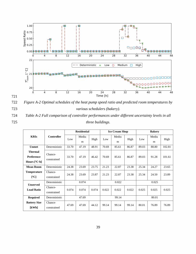
Figure A-2 Optimal schedules of the heat pump speed ratio and predicted room temperatures by 722
various schedulers (bakery). 723
Table A-2 Full comparison of controller performances under different uncertainty levels in all 724
three buildings. 725
KRIs Controller
Residential Ice Cream Shop Bakery
Low Mediu
m High Low
Mediu
m High Low
Mediu
m High
Unmet
Thermal
Preference
Hours [ºC·h]
Deterministic 33.70 47.19 48.91 70.69 85.61 86.87 89.03 88.80 102.81
Chance-
constrained 33.70 47.19 46.42 70.69 85.61 86.87 89.03 91.28 101.61
Mean Room
Temperature
[ºC]
Deterministic 24.38 23.69 23.75 21.23 22.87 23.38 25.34 24.27 23.65
Chance-
constrained 24.38 23.69 23.87 21.23 22.87 23.38 25.34 24.50 23.89
Unserved
Load Ratio
Deterministic 0.074 0.022 0.025
Chance-
constrained 0.074 0.074 0.074 0.022 0.022 0.022 0.025 0.025 0.025
Required
Battery Size
[kWh]
Deterministic 47.69 99.14 80.01
Chance-
constrained 47.69 47.69 44.12 99.14 99.14 99.14 80.01 76.89 76.89

40
References 726
[1] The Texas Tribune. Winter Storm 2021. https://www.texastribune.org/series/winter-storm-727
power-outage/ (accessed Apr 1, 2021). 728
[2] Wang, J.; Garifi, K.; Baker, K.; Zuo, W.; Zhang, Y. Optimal Operation for Resilient 729
Communities through a Hierarchical Load Scheduling Framework. In Proceedings of 2020 730
Building Performance Analysis Conference & SimBuild; Virtual Conference, 2020. 731
[3] Wang, J.; Zuo, W.; Rhode-Barbarigos, L.; Lu, X.; Wang, J.; Lin, Y. Literature Review on 732
Modeling and Simulation of Energy Infrastructures from a Resilience Perspective. Reliab. 733
Eng. Syst. Saf., 2019, 183, 360–373. https://doi.org/10.1016/j.ress.2018.11.029. 734
[4] Tang, H.; Wang, S.; Li, H. Flexibility Categorization, Sources, Capabilities and 735
Technologies for Energy-Flexible and Grid-Responsive Buildings: State-of-The-Art and 736
Future Perspective. Energy, 2020, 119598. https://doi.org/10.1016/j.energy.2020.119598. 737
[5] Kou, X.; Li, F.; Dong, J.; Olama, M.; Starke, M.; Chen, Y.; Zandi, H. A Comprehensive 738
Scheduling Framework Using SP-ADMM for Residential Demand Response with Weather 739
and Consumer Uncertainties. IEEE Trans. Power Syst., 2020. 740
https://doi.org/10.1109/TPWRS.2020.3029272. 741
[6] Faraji, J.; Ketabi, A.; Hashemi-Dezaki, H.; Shafie-Khah, M.; Catalão, J. P. S. Optimal Day-742
Ahead Self-Scheduling and Operation of Prosumer Microgrids Using Hybrid Machine 743
Learning-Based Weather and Load Forecasting. IEEE Access, 2020, 8, 157284–157305. 744
https://doi.org/10.1109/ACCESS.2020.3019562. 745
[7] Wang, J.; Garifi, K.; Baker, K.; Zuo, W.; Zhang, Y.; Huang, S.; Vrabie, D. Optimal 746
Renewable Resource Allocation and Load Scheduling of Resilient Communities. Energies. 747
2020. https://doi.org/10.3390/en13215683. 748
[8] Yu, M. G.; Pavlak, G. S. Assessing the Performance of Uncertainty-Aware Transactive 749
Controls for Building Thermal Energy Storage Systems. Appl. Energy, 2021, 282, 116103. 750

41
https://doi.org/10.1016/j.apenergy.2020.116103. 751
[9] Liang, Z.; Huang, C.; Su, W.; Duan, N.; Donde, V.; Wang, B.; Zhao, X. Safe Reinforcement 752
Learning-Based Resilient Proactive Scheduling for a Commercial Building Considering 753
Correlated Demand Response. IEEE Open Access J. Power Energy, 2021, 8, 85–96. 754
https://doi.org/10.1109/oajpe.2021.3064319. 755
[10] Ahmad, A.; Khan, J. Y. Real-Time Load Scheduling, Energy Storage Control and Comfort 756
Management for Grid-Connected Solar Integrated Smart Buildings. Appl. Energy, 2020, 757
259, 114208. https://doi.org/10.1016/j.apenergy.2019.114208. 758
[11] E Silva, D. P.; Salles, J. L. F.; Fardin, J. F.; Pereira, M. M. R. Management of an Island and 759
Grid-Connected Microgrid Using Hybrid Economic Model Predictive Control with 760
Weather Data. Appl. Energy, 2020, 278, 115581. 761
https://doi.org/10.1016/j.apenergy.2020.115581. 762
[12] Yundra, E.; Surabaya, U. N.; Kartini, U.; Wardani, L.; Ardianto, D.; Surabaya, U. N.; 763
Surabaya, U. N.; Surabaya, U. N. Hybrid Model Combined Fuzzy Multi-Objective Decision 764
Making with Feed Forward Neural Network (F-MODMFFNN) For Very Short-Term Load 765
Forecasting Based on Weather Data. Int. J. Intell. Eng. Syst., 2020, 13 (4), 182–195. 766
https://doi.org/10.22266/IJIES2020.0831.16. 767
[13] Garifi, K.; Baker, K.; Christensen, D.; Touri, B. Stochastic Home Energy Management 768
Systems with Varying Controllable Resources. In 2019 IEEE Power & Energy Society 769
General Meeting (PESGM); IEEE: Atlanta, GA, USA, 2019; pp 1–5. 770
[14] Lu, M.; Abedinia, O.; Bagheri, M.; Ghadimi, N.; Shafie‐khah, M.; Catalão, J. P. S. Smart 771
Load Scheduling Strategy Utilising Optimal Charging of Electric Vehicles in Power Grids 772
Based on an Optimisation Algorithm. IET Smart Grid, 2020, 3 (6), 914–923. 773
https://doi.org/10.1049/iet-stg.2019.0334. 774
[15] Khalid, Z.; Abbas, G.; Awais, M.; Alquthami, T.; Rasheed, M. B. A Novel Load Scheduling 775
Mechanism Using Artificial Neural Network Based Customer Profiles in Smart Grid. 776

42
Energies, 2020, 13 (5), 1062. https://doi.org/10.3390/en13051062. 777
[16] Kerboua, A.; Boukli-Hacene, F.; Mourad, K. A. Particle Swarm Optimization for Micro-778
Grid Power Management and Load Scheduling. Int. J. Energy Econ. Policy, 2020, 10 (2), 779
71. https://doi.org/10.32479/ijeep.8568. 780
[17] Kaur, R.; Schaye, C.; Thompson, K.; Yee, D. C.; Zilz, R.; Sreenivas, R. S.; Sowers, R. B. 781
Machine Learning and Price-Based Load Scheduling for an Optimal IoT Control in the 782
Smart and Frugal Home. Energy AI, 2021, 3, 100042. 783
https://doi.org/10.1016/j.egyai.2020.100042. 784
[18] Chung, H.-M.; Maharjan, S.; Zhang, Y.; Eliassen, F. Distributed Deep Reinforcement 785
Learning for Intelligent Load Scheduling in Residential Smart Grids. IEEE Trans. Ind. 786
Informatics, 2020, 17 (4), 2752–2763. https://doi.org/10.1109/TII.2020.3007167. 787
[19] Aftab, M.; Chen, C.; Chau, C.-K.; Rahwan, T. Automatic HVAC Control with Real-Time 788
Occupancy Recognition and Simulation-Guided Model Predictive Control in Low-Cost 789
Embedded System. Energy Build., 2017, 154, 141–156. 790
https://doi.org/10.1016/j.enbuild.2017.07.077. 791
[20] Lim, B.; Van Den Briel, M.; Thiébaux, S.; Backhaus, S.; Bent, R. HVAC-Aware Occupancy 792
Scheduling. In Proceedings of the AAAI Conference on Artificial Intelligence; 2015; Vol. 793
29. 794
[21] Jin, Y.; Yan, D.; Zhang, X.; An, J.; Han, M. A Data-Driven Model Predictive Control for 795
Lighting System Based on Historical Occupancy in an Office Building: Methodology 796
Development. In Building Simulation; Springer, 2020; pp 1–17. 797
https://doi.org/10.1007/s12273-020-0638-x. 798
[22] Wang, J.; Zuo, W.; Huang, S.; Vrabie, D. Data-Driven Prediction of Occupant Presence and 799
Lighting Power: A Case Study for Small Commercial Buildings. In American Modelica 800
Conference; 2020. 801

43
[23] Chen, X.; Wang, Q.; Srebric, J. Model Predictive Control for Indoor Thermal Comfort and 802
Energy Optimization Using Occupant Feedback. Energy Build., 2015, 102, 357–369. 803
https://doi.org/10.1016/j.enbuild.2015.06.002. 804
[24] West, S. R.; Ward, J. K.; Wall, J. Trial Results from a Model Predictive Control and 805
Optimisation System for Commercial Building HVAC. Energy Build., 2014, 72, 271–279. 806
https://doi.org/10.1016/j.enbuild.2013.12.037. 807
[25] Drgoňa, J.; Arroyo, J.; Figueroa, I. C.; Blum, D.; Arendt, K.; Kim, D.; Ollé, E. P.; Oravec, 808
J.; Wetter, M.; Vrabie, D. L. All You Need to Know about Model Predictive Control for 809
Buildings. Annu. Rev. Control, 2020. https://doi.org/10.1016/j.arcontrol.2020.09.001. 810
[26] Garifi, K.; Baker, K.; Touri, B.; Christensen, D. Stochastic Model Predictive Control for 811
Demand Response in a Home Energy Management System. In 2018 IEEE Power & Energy 812
Society General Meeting (PESGM); Portland, OR, USA, 2018; pp 1–5. 813
[27] Zhang, X.; Schildbach, G.; Sturzenegger, D.; Morari, M. Scenario-Based MPC for Energy-814
Efficient Building Climate Control under Weather and Occupancy Uncertainty. In 2013 815
European Control Conference (ECC); IEEE, 2013; pp 1029–1034. 816
[28] He, D.; Huang, S.; Zuo, W.; Kaiser, R. Towards to the Development of Virtual Testbed for 817
Net Zero Energy Communities. In SimBuild 2016: Building Performance Modeling 818
Conference; Salt Lake City, UT, USA, 2016; Vol. 6. 819
[29] Zakula, T.; Armstrong, P. R.; Norford, L. Modeling Environment for Model Predictive 820
Control of Buildings. Energy Build., 2014, 85, 549–559. 821
https://doi.org/10.1016/j.enbuild.2014.09.039. 822
[30] The Engineering ToolBox. Metabolic Heat Gain from Persons. 823
https://www.engineeringtoolbox.com/metabolic-heat-persons-d_706.html (accessed Feb 824
19, 2021). 825
[31] Hosni, M. H.; Beck, B. T. Updated Experimental Results for Heat Gain from Office 826

44
Equipment in Buildings. ASHRAE Trans., 2011, 117 (2). 827
[32] ASHRAE. ASHRAE Handbook — Fundamentals 2017; 2017. 828
[33] Lawrence Berkeley National Laboratory. Home Energy Saver & Score: Engineering 829
Documentation - Internal Gains. http://hes-documentation.lbl.gov/calculation-830
methodology/calculation-of-energy-consumption/heating-and-cooling-831
calculation/internal-gains (accessed Feb 16, 2021). 832
[34] Maslow, A. H. Motivation and Personality; Harper & Brothers: New York City, USA, 1954. 833
[35] Roth, A.; Reyna, J.; Christensen, J.; Vrabie, D.; Adetola, V. GEB Technical Report Webinar 834
Series: Whole-Building Control, Sensing, Modeling & Analytics 835
https://www.energy.gov/sites/default/files/2020/05/f74/bto-geb-webinar-CSMA-836
051920.pdf. 837
[36] Zhao, Z.; Lee, W. C.; Shin, Y.; Song, K.-B. An Optimal Power Scheduling Method for 838
Demand Response in Home Energy Management System. IEEE Trans. Smart Grid, 2013, 839
4 (3), 1391–1400. https://doi.org/10.1109/TSG.2013.2251018. 840
[37] SiteSage. Historic Green Village Submetering Data. 841
https://sitesage.net/home/management/index.php (accessed Oct 7, 2020). 842
[38] Garifi, K.; Baker, K.; Christensen, D.; Touri, B. Control of home energy management 843
systems with energy storage: Nonsimultaneous charging and discharging guarantees 844
https://arxiv.org/pdf/1805.00100.pdf. 845
[39] Gunay, H. B.; O’Brien, W.; Beausoleil-Morrison, I.; Bursill, J. Development and 846
Implementation of a Thermostat Learning Algorithm. Sci. Technol. Built Environ., 2018, 847
24 (1), 43–56. https://doi.org/10.1080/23744731.2017.1328956. 848
[40] Heirung, T. A. N.; Paulson, J. A.; O’Leary, J.; Mesbah, A. Stochastic Model Predictive 849
Control—How Does It Work? Comput. Chem. Eng., 2018, 114, 158–170. 850
https://doi.org/10.1016/j.compchemeng.2017.10.026. 851

45
[41] The Modelica Association. Modelica. 2019. 852
[42] Huang, S.; Wang, J.; Fu, Y.; Zuo, W.; Hinkelman, K.; Kaiser, M. R.; He, D.; Vrabie, D. An 853
Open-Source Virtual Testbed for a Real Net-Zero Energy Community; 2021. 854
[43] Mooney, C. Z. Monte Carlo Simulation; Sage, 1997. 855
[44] Statistics Solutions. Chi-Square Goodness of Fit Test. 856
https://www.statisticssolutions.com/chi-square-goodness-of-fit-test/ (accessed Feb 25, 857
2021). 858
[45] Chen, Y.; Hong, T.; Luo, X. An Agent-Based Stochastic Occupancy Simulator. In Building 859
Simulation; Springer, 2018; Vol. 11, pp 37–49. 860
861