j tseng october 22, 2019 - university of oxfordtseng/teaching/b2/b2-lectures-2018.pdf · b2:...
TRANSCRIPT

B2: Symmetry and Relativity
J Tseng
October 22, 2019

Contents
1 Introduction 2
1.1 Books . . . . . . . . . . . . . . . . . . . . . . . . . . . . . . . . . . . . . . . 2
1.2 Postulates . . . . . . . . . . . . . . . . . . . . . . . . . . . . . . . . . . . . . 2
1.3 *Vector transformation . . . . . . . . . . . . . . . . . . . . . . . . . . . . . . 3
1.4 Symmetry and relativity . . . . . . . . . . . . . . . . . . . . . . . . . . . . . 4
1.5 Units . . . . . . . . . . . . . . . . . . . . . . . . . . . . . . . . . . . . . . . . 5
1.5.1 Other conventions . . . . . . . . . . . . . . . . . . . . . . . . . . . . . 5
1.6 4-vector basics . . . . . . . . . . . . . . . . . . . . . . . . . . . . . . . . . . . 5
1.7 *Invariants . . . . . . . . . . . . . . . . . . . . . . . . . . . . . . . . . . . . . 7
1.8 Spacetime diagrams . . . . . . . . . . . . . . . . . . . . . . . . . . . . . . . . 8
1.8.1 *Proper time . . . . . . . . . . . . . . . . . . . . . . . . . . . . . . . 8
1.9 Basic 4-vectors . . . . . . . . . . . . . . . . . . . . . . . . . . . . . . . . . . 9
1.9.1 Position . . . . . . . . . . . . . . . . . . . . . . . . . . . . . . . . . . 9
1.9.2 Velocity . . . . . . . . . . . . . . . . . . . . . . . . . . . . . . . . . . 9
1.9.3 Acceleration . . . . . . . . . . . . . . . . . . . . . . . . . . . . . . . . 10
1.9.4 Momentum . . . . . . . . . . . . . . . . . . . . . . . . . . . . . . . . 10
1.9.5 Force . . . . . . . . . . . . . . . . . . . . . . . . . . . . . . . . . . . . 11
2 Applications of 4-momentum 12
2.1 *Conservation of energy-momentum . . . . . . . . . . . . . . . . . . . . . . . 12
2.2 *Annihilation, decay, and formation . . . . . . . . . . . . . . . . . . . . . . . 12
2.2.1 *Center of momentum frame . . . . . . . . . . . . . . . . . . . . . . . 12
2.2.2 Decay at rest . . . . . . . . . . . . . . . . . . . . . . . . . . . . . . . 13
2.2.3 In-flight decay . . . . . . . . . . . . . . . . . . . . . . . . . . . . . . . 14
2.3 *Collisions . . . . . . . . . . . . . . . . . . . . . . . . . . . . . . . . . . . . . 15
1

B2: Symmetry and Relativity J Tseng
2.3.1 Absorption . . . . . . . . . . . . . . . . . . . . . . . . . . . . . . . . 15
2.3.2 Particle formation . . . . . . . . . . . . . . . . . . . . . . . . . . . . . 16
2.3.3 *Compton scattering . . . . . . . . . . . . . . . . . . . . . . . . . . . 18
3 Force 20
3.1 Pure force . . . . . . . . . . . . . . . . . . . . . . . . . . . . . . . . . . . . . 20
3.2 Transformation of force . . . . . . . . . . . . . . . . . . . . . . . . . . . . . . 21
3.3 *Force and simple motion problems . . . . . . . . . . . . . . . . . . . . . . . 22
3.3.1 Motion under pure force . . . . . . . . . . . . . . . . . . . . . . . . . 22
3.3.2 Linear motion . . . . . . . . . . . . . . . . . . . . . . . . . . . . . . . 23
3.3.3 Hyperbolic motion . . . . . . . . . . . . . . . . . . . . . . . . . . . . 24
3.3.4 Constant external force . . . . . . . . . . . . . . . . . . . . . . . . . . 25
3.3.5 Circular motion . . . . . . . . . . . . . . . . . . . . . . . . . . . . . . 26
4 Lagrangians 28
4.1 *Equations of particle motion from the Lagrangian . . . . . . . . . . . . . . 28
4.1.1 Central force problem . . . . . . . . . . . . . . . . . . . . . . . . . . . 31
5 Further kinematics 34
5.1 *Doppler effect . . . . . . . . . . . . . . . . . . . . . . . . . . . . . . . . . . 34
5.2 *Aberration . . . . . . . . . . . . . . . . . . . . . . . . . . . . . . . . . . . . 36
5.3 Headlight effect . . . . . . . . . . . . . . . . . . . . . . . . . . . . . . . . . . 36
5.4 Generators . . . . . . . . . . . . . . . . . . . . . . . . . . . . . . . . . . . . . 37
5.5 Thomas precession . . . . . . . . . . . . . . . . . . . . . . . . . . . . . . . . 40
6 Scalars, Vectors, and Tensors 43
6.1 Generalized Lorentz transformation . . . . . . . . . . . . . . . . . . . . . . . 43
6.1.1 Index notation . . . . . . . . . . . . . . . . . . . . . . . . . . . . . . 43
6.1.2 Summation convention . . . . . . . . . . . . . . . . . . . . . . . . . . 45
6.1.3 Metric . . . . . . . . . . . . . . . . . . . . . . . . . . . . . . . . . . . 45
6.2 Lorentz transformation matrices . . . . . . . . . . . . . . . . . . . . . . . . . 46
6.3 Tensors . . . . . . . . . . . . . . . . . . . . . . . . . . . . . . . . . . . . . . 48
6.4 *4-gradient . . . . . . . . . . . . . . . . . . . . . . . . . . . . . . . . . . . . 49
2

B2: Symmetry and Relativity J Tseng
7 Groups 51
7.1 Example: permutation group . . . . . . . . . . . . . . . . . . . . . . . . . . 52
7.2 Rotations . . . . . . . . . . . . . . . . . . . . . . . . . . . . . . . . . . . . . 53
7.3 Representations . . . . . . . . . . . . . . . . . . . . . . . . . . . . . . . . . . 54
7.3.1 Orthogonal matrices . . . . . . . . . . . . . . . . . . . . . . . . . . . 54
7.3.2 Spinor representation . . . . . . . . . . . . . . . . . . . . . . . . . . . 59
7.3.3 Spinor representation space . . . . . . . . . . . . . . . . . . . . . . . 60
7.3.4 Spinor representation with matrices . . . . . . . . . . . . . . . . . . . 62
7.3.5 Higher-spin representations . . . . . . . . . . . . . . . . . . . . . . . 63
8 Lorentz group 65
8.1 Commutators . . . . . . . . . . . . . . . . . . . . . . . . . . . . . . . . . . . 66
8.2 Fundamental representations . . . . . . . . . . . . . . . . . . . . . . . . . . . 67
8.2.1 Direct product representations . . . . . . . . . . . . . . . . . . . . . . 72
8.3 Space inversion . . . . . . . . . . . . . . . . . . . . . . . . . . . . . . . . . . 73
9 Poincare group 75
9.1 Casimir operators . . . . . . . . . . . . . . . . . . . . . . . . . . . . . . . . . 77
9.2 Representation space of the Poincare group . . . . . . . . . . . . . . . . . . . 78
9.2.1 Supersymmetry and spacetime . . . . . . . . . . . . . . . . . . . . . . 79
9.3 Physics tensors . . . . . . . . . . . . . . . . . . . . . . . . . . . . . . . . . . 80
9.3.1 3D tensors . . . . . . . . . . . . . . . . . . . . . . . . . . . . . . . . . 80
9.3.2 *Transformation of electromagnetic fields . . . . . . . . . . . . . . . . 80
9.3.3 *The Maxwell field tensor . . . . . . . . . . . . . . . . . . . . . . . . 82
10 Classical fields 84
10.1 The field viewpoint . . . . . . . . . . . . . . . . . . . . . . . . . . . . . . . . 84
10.2 Continuous systems . . . . . . . . . . . . . . . . . . . . . . . . . . . . . . . . 85
10.3 Lagrangian density . . . . . . . . . . . . . . . . . . . . . . . . . . . . . . . . 86
11 Relativistic field equations 90
11.1 *Classical Klein-Gordon equation . . . . . . . . . . . . . . . . . . . . . . . . 90
11.1.1 Complex-valued fields . . . . . . . . . . . . . . . . . . . . . . . . . . 92
11.2 Dirac equation . . . . . . . . . . . . . . . . . . . . . . . . . . . . . . . . . . 93
3

B2: Symmetry and Relativity J Tseng
11.3 Weyl equation . . . . . . . . . . . . . . . . . . . . . . . . . . . . . . . . . . . 96
12 Electromagnetism 97
12.1 Revision: Maxwell’s equations and potentials . . . . . . . . . . . . . . . . . . 97
12.2 *Electromagnetic potential as a 4-vector . . . . . . . . . . . . . . . . . . . . 97
12.3 *Gauge invariance . . . . . . . . . . . . . . . . . . . . . . . . . . . . . . . . . 100
12.4 Lagrangian for em fields, equations of motion . . . . . . . . . . . . . . . . . 101
12.4.1 Use of invariants . . . . . . . . . . . . . . . . . . . . . . . . . . . . . 102
12.4.2 Motion in an electromagnetic field . . . . . . . . . . . . . . . . . . . . 104
13 Radiation 106
13.1 Conservation of energy . . . . . . . . . . . . . . . . . . . . . . . . . . . . . . 106
13.2 Plane waves in vacuum . . . . . . . . . . . . . . . . . . . . . . . . . . . . . . 107
14 Fields with sources 110
14.1 *Fields of a uniformly moving charge . . . . . . . . . . . . . . . . . . . . . . 110
14.2 *Retarded potentials . . . . . . . . . . . . . . . . . . . . . . . . . . . . . . . 111
14.3 Arbitrarily moving charge . . . . . . . . . . . . . . . . . . . . . . . . . . . . 115
15 Accelerated charge 118
15.1 Slowly oscillating dipole . . . . . . . . . . . . . . . . . . . . . . . . . . . . . 118
15.2 *Field of an accelerated charge (details) . . . . . . . . . . . . . . . . . . . . 120
15.3 *Half-wave electric dipole antenna . . . . . . . . . . . . . . . . . . . . . . . . 123
15.3.1 *Radiated power . . . . . . . . . . . . . . . . . . . . . . . . . . . . . 124
15.3.2 Energy loss in accelerators . . . . . . . . . . . . . . . . . . . . . . . . 127
16 Energy-momentum tensor 128
16.1 Fluid examples . . . . . . . . . . . . . . . . . . . . . . . . . . . . . . . . . . 129
16.2 *Energy-momentum tensor of the EM field . . . . . . . . . . . . . . . . . . . 130
16.3 *Applications with simple geometries . . . . . . . . . . . . . . . . . . . . . . 131
16.3.1 *Parallel-plate capacitor . . . . . . . . . . . . . . . . . . . . . . . . . 131
16.3.2 *Long straight solenoid . . . . . . . . . . . . . . . . . . . . . . . . . . 131
16.3.3 *Plane waves . . . . . . . . . . . . . . . . . . . . . . . . . . . . . . . 132
17 Noether’s theorem 133
4

B2: Symmetry and Relativity J Tseng
17.1 Discrete systems . . . . . . . . . . . . . . . . . . . . . . . . . . . . . . . . . 133
17.1.1 Action invariance . . . . . . . . . . . . . . . . . . . . . . . . . . . . . 134
17.1.2 On-shell variation . . . . . . . . . . . . . . . . . . . . . . . . . . . . . 134
17.1.3 Noether’s Theorem . . . . . . . . . . . . . . . . . . . . . . . . . . . . 135
17.1.4 Examples . . . . . . . . . . . . . . . . . . . . . . . . . . . . . . . . . 136
17.2 Noether’s Theorem for classical fields . . . . . . . . . . . . . . . . . . . . . . 140
17.2.1 Translations . . . . . . . . . . . . . . . . . . . . . . . . . . . . . . . . 141
17.2.2 Complex fields . . . . . . . . . . . . . . . . . . . . . . . . . . . . . . 142
17.2.3 Maxwell’s equations . . . . . . . . . . . . . . . . . . . . . . . . . . . 144
17.3 Local gauge invariance . . . . . . . . . . . . . . . . . . . . . . . . . . . . . . 146
5
Chapter 1
Introduction
These notes are in the process of construction. Comments, clarifications, and especiallycorrections, are welcome by the author.
1.1 Books
The main text for the course is AM Steane, Relativity Made Relatively Easy, Oxford Uni-versity Press, 2012.
However, I’ve also drawn on quite a few other sources, including
• JD Jackson, Classical Electrodynamics, Wiley, 1975.
• H Goldstein, Classical Mechanics, Addison Wesley, 1980.
• WK Tung, Group Theory in Physics, World Scientific, 1985.
• lots of Oxford lecture notes, especially from AM Steane, CWP Palmer, S Balbus, andJ Binney.
In some cases, there are more recent editions of these textbooks.
1.2 Postulates
Postulates:
1. Principle of RelativityThe motions of bodies included in a given space are the same among themselves,whether that space is at rest or moves uniformly (forward) in a straight line.
• The laws of physics take the same mathematical form in all inertial frames ofreference.
6

B2: Symmetry and Relativity J Tseng
2. Light speed postulateThere is a finite maximum speed for signals.
• There is an inertial frame in which the speed of light in vacuum is independentof the motion of the source.
Additional postulates (or assumptions):
1. Flat space, sometimes called “Euclidean”.
2. Internal interactions in an isolated system cannot change the system’s total momentum.
• or translational symmetry, for reasons which will be developed later.
1.3 *Vector transformation
(Newtonian and relativistic)
We’ll use “frame” in the sense of a coordinate system in space and time. Since we usually talkof “points” as having spatial coordinates, we’ll call events with space and time coordinates“events”. I will omit discussion of these concepts in terms of light signals and bouncing offmirrors, as these discussions can obscure the essential simplicity of coordinate systems.
We also draw a distinction between events and when they’re observed: it may take time foryou to observe an event (in other words, observe its consequences), but once you do, you maybe able to deduce the event’s spacetime coordinates. So, for instance, we lost contact with theCassini mission as it plunged into Saturn’s atmosphere at 4.55am PDT on 15 September, butwe knew that the last signal which could reach us was actually transmitted around 3.32amPDT. By the time we received its last transmission, it had already been vaporized for almost1.5 hours.
Standard configuration: we have two frames, S and S ′, with all spatial axes parallel. S ′ thenmoves with a constant speed in the x direction with respect to S.
Galilean (Newtonian) transformation between inertial frames in standard configuration:
t′ = t (1.1)
x′ = x− vt (1.2)
y′ = y (1.3)
z′ = z (1.4)
where v is the constant speed.
Lorentz transformation for standard configuration:
t′ = γ(t− vx
c2
)(1.5)
x′ = γ(x− vt) (1.6)
y′ = y (1.7)
z′ = z (1.8)
7

B2: Symmetry and Relativity J Tseng
where γ = (1− β2)−1/2.
There are a number of derivations of the Lorentz transformation, and you can find some inbasic texts in Special Relativity or your CP1 notes. The physics hasn’t changed.
1.4 Symmetry and relativity
The idea of symmetry: transformations which do not change the physics. This is basically thefirst postulate of Special Relativity: equations of motion remain unchanged by the Lorentztransformation.
Consider first one of the first equations of motion in physics, the Newtonian equation for afree particle:
0 = f = md2x
dt2(1.9)
If we plug in the Galilean transformation,
md2x′
dt′2= m
d2
dt2(x− vt) = m
d
dt
(dx
dt− v)
= md2x
dt2= 0 (1.10)
so we see the equation of motion is unchanged by the transformation.
This isn’t the only symmetry of Newtonian physics. For instance, consider a rotation in thexy plane:
t′ = t (1.11)
x′ = x cos θ − y sin θ (1.12)
y′ = x sin θ + y cos θ (1.13)
z′ = z (1.14)
(1.15)
This also leaves Newton’s law invariant, at least in vector form. It also does somethingmore: it leaves the lengths of all displacements the same. So we can rotate the world (orthe experiment), and all equations which involve vector displacements are left unchanged.(Note that the same can’t be said of Galilean transformations.)
The Lorentz transformation, however, does change the form of the Newton equation of mo-tion. Since we are led to believe that the Lorentz transformation is the proper transformationof space and time coordinates, then it must be that Newton’s Law is the one which must bemodified: it must be a low-velocity approximation of a better equation of motion.
In this course, one of the things we’ll be doing is exploring the implications of the requirementthat physics is unchanged by the Lorentz transformation. On the one hand, we require thatall physics, ultimately, be invariant under a Lorentz transformation. On the other hand, wealso want to find out everything which is invariant under such transformations, to see if wecan then observe them in Nature. This may also apply to other possible symmetries.
In other words, and more generally, we’ll look for what physics tells us about symmetry, andwhat symmetry tells us about physics.
8
B2: Symmetry and Relativity J Tseng
1.5 Units
First, let’s rephrase the Lorentz transformation by moving our c’s around:
ct′ = γ(ct− βx) (1.16)
x′ = γ(x− βct) (1.17)
y′ = y (1.18)
z′ = z (1.19)
This makes the equations look more alike, if you take ct as the time-like coordinate. And ofcourse ct now has units of length, as the others already do.
1.5.1 Other conventions
Different textbooks will take different approaches to making these equations look symmetric,so it’s worth a word of warning.
• Natural units: just assign c = 1. This basically says that length and time are reallythe same unit, which in a sense is true. And indeed this is how most particle physicists(for instance) work, even to the extent that we’ll talk about the “lifetime” of a bottomquark meson to be “about 450 microns”. And indeed you can also assign ~ = 1.If you’ve followed all your units through correctly, you can just reintroduce howevermany c’s and ~’s as you need to the final result to get the units you need, and itworks perfectly. But it can be confusing to students, so for the lectures I’ll try to avoidit. However, if I lapse into it (because it’s how I normally work), well, apologies inadvance.
• Many older textbooks also make the time component imaginary. This makes thecoordinates really symmetric: the Lorentz boost now really looks like a Euclideanrotation. Most modern textbooks consider this a step too far, because it still remainsthat time is special—whatever units you use for it. We’ll use another way to pick outthe special behavior of time. Importantly, it’s the way which will extend naturally togeneral relativity.
1.6 4-vector basics
Now let’s return to the Lorentz transformation itself. The form looks remarkably like arotation: the component being transformed is always multipled by the same factor γ, whilethe component being mixed in multiplied by another factor −βγ. To see this more clearly,let’s reformulate the transformations in terms of vectors and matrices. I believe you willhave run into this in CP1, even though it only gets on the syllabus for this paper.
We construct a 4-dimensional vector using the following convention:
X = (ct,x) (1.20)
9

B2: Symmetry and Relativity J Tseng
where you can see that we tend to list the time component first (the “zeroth” component—this makes it more natural for programming in most modern programming languages, bythe way). Since you are probably also used to thinking of vectors as single-width columnmatrices,
X =
ctxyz
(1.21)
A spatial rotation then looks as follows:
X′ =
ct′
x′
y′
z′
=
1 0 0 00 cos θ − sin θ 00 sin θ cos θ 00 0 0 1
ctxyz
= RX (1.22)
and a Lorentz transformation
X′ =
ct′
x′
y′
z′
=
γ −βγ 0 0−βγ γ 0 0
0 0 1 00 0 0 1
ctxyz
= LX (1.23)
which can be written in a more suggestive form:
X′ =
ct′
x′
y′
z′
=
cosh η − sinh η 0 0− sinh η cosh η 0 0
0 0 1 00 0 0 1
ctxyz
= LX (1.24)
You can confirm that the trigonometric identities for cosh η and sinh η reproduce that ofγ and βγ. Now this looks a lot more like a rotation, but instead of mixing two spacecoordinates, it mixes time and a space coordinate. In fact, it’s like a rotation through animaginary angle, which reflects that time still has a special place different from space.
The parameter η is called “rapidity”, and it has another nice property, which is that additionof parallel velocities is easy. There are two ways to see this. First, you can multiply out twoLorentz transformations for two rapidities η and η′. (I’ll do this with 2 × 2 matrices, sinceit leaves the other components unchanged.)(
cosh η′ − sinh η′
− sinh η′ cosh η′
)(cosh η − sinh η− sinh η cosh η
)(1.25)
=
(cosh η′ cosh η + sinh η′ sinh η − cosh η′ sinh η − sinh η′ cosh η− cosh η′ sinh η − sinh η′ cosh η cosh η′ cosh η + sinh η′ sinh η
)(1.26)
=
(cosh(η′ + η) − sinh(η′ + η)− sinh(η′ + η) cosh(η′ + η)
)(1.27)
The other way is simpler: notice that β = tanh η. The addition formula is then just thehyperbolic tangent addition formula:
tanh η′′ = tanh(η + η′) =tanh η + tanh η′
1 + tanh η tanh η′(1.28)
10

B2: Symmetry and Relativity J Tseng
1.7 *Invariants
The dot product between the two 4-vectors is defined with a slight wrinkle which handlesthe special behavior of time:
A · B = ATgB (1.29)
where
g =
−1 0 0 00 1 0 00 0 1 00 0 0 1
(1.30)
so the norm or “length” of a 4-vector is
X · X = −(ct)2 + x · x (1.31)
which should be familiar to you as the invariant separation between space-time events. Thematrix g is called the “metric”.
But to see whether this is true, let’s do an explicit calculation of the dot product, justconcentrating on the 2×2 again. Remember, though, we need to apply the Lorentz transformΛ to both vectors, since we want to put the whole system into another frame, not just onepart.
(ΛA) · (ΛB) = (ATΛT )g(ΛB) = AT (ΛTgΛ)B (1.32)
The parenthesis is then
ΛTgΛ =
(cosh η − sinh η− sinh η cosh η
)(−1 00 1
)(cosh η − sinh η− sinh η cosh η
)(1.33)
=
(− cosh η − sinh ηsinh η cosh η
)(cosh η − sinh η− sinh η cosh η
)(1.34)
=
(− cosh2 η + sinh2 η 0
0 − sinh2 η + cosh2 η
)(1.35)
=
(−1 00 1
)(1.36)
which is simply g again, so we come to
(ΛA) · (ΛB) = (ATΛT )g(ΛB) = ATgB (1.37)
Thus the dot product is invariant. A corollary is that the norm of the interval is invariant,as we expected.
The example we’ve worked with is fairly specific to the standard configuration, but it’sstraightforward to generalize once we have it in matrix form. In fact, we can define theLorentz transformation generically in terms of the metric, in that it’s any matrix Λ whichsatisfies the equation
ΛTgΛ = g (1.38)
It then becomes a pre-requisite that any equation which purports to be consistent withSpecial Relativity (“covariant”, but perhaps more accurately “form-invariant” or simply“invariant”) can be written in terms of quantities that transform using such a Λ.
11

B2: Symmetry and Relativity J Tseng
1.8 Spacetime diagrams
A spacetime diagram shows time as another axis. Since four dimensions can be hard tovisualize, we often make illustrations with just x and t.
First, let’s look at the features related to the interval s2 = −c2∆t2 + ∆x2, relative to theorigin:
• the null intervals: s2 = 0. This is how light travels.
• time-like intervals: s2 < 0, so the time difference is larger than the space distance.These intervals can be causally connected, in the sense that there’s enough time forthe past end to affect the future end.
• space-like intervals: s2 > 0. These intervals cannot be causally connected; there’s notenough time for a signal to reach one from the other.
Lines of simultaneity are parallel to the x axis (think of measuring the length of rod: it’sa difference on the x axis, where the two measuring events have to be at the same t in theframe). Their intersection with the t axis determines their ordering in time.
A worldline is a trajectory of a physical body. Each segment on the worldline is causallyconnected with the previous segment.
A Lorentz transformation (“boost”) pushes the x and t axes closer to the null line. Thisshouldn’t be surprising, since the ultimate boost to light speed should put you on the nullline. We can see that the time-like, space-like, and null categories are invariants, i.e., atime-like interval stays time-like in any frame.
1.8.1 *Proper time
Lines of simultaneity remain parallel to the transformed x′ axis. This means that the orderof causally connected events is also an invariant.
This enables us to parameterize the worldline in terms of some monotonically increasingfunction. The most convenient is the proper time, which is the time experienced by thebody in its own rest frame.
Another way of looking at it is that proper time measures a body’s path along its ownworldline, since a body at rest has ∆τ 2 = −s2 = ∆t2. The negative sign is an artefact of themetric we’ve chosen.
The relationship between proper time and that of any frame can be found by consideringthe Lorentz transformation, starting from the rest frame:
ct = γ(cτ − βx) (1.39)
resulting in (choosing x = 0 for the body in its own rest frame)
dt
dτ= γ (1.40)
12

B2: Symmetry and Relativity J Tseng
This is actually the familiar time dilation. When written as
dt = γdτ (1.41)
we see, for instance, why we see cosmic ray muons live (and travel) much longer than theone microsecond they should live in their own rest frame.
1.9 Basic 4-vectors
Let’s look at a few basic 4-vectors.
1.9.1 Position
Position and displacement:X = (ct,x) (1.42)
The invariant is the usual invariant interval (possibly with a minus sign), which is also thebody’s proper time
X · X = −c2t2 + x · x = −c2τ 2 (1.43)
The easiest way to see this is to evaluate the dot product in the body’s rest frame.
1.9.2 Velocity
Velocity:
U =dX
dτ=
(cdt
dτ,dx
dt
dt
dτ
)= γ(c,u) (1.44)
The invariant is the same for all 4-velocities:
U · U = γ2(−c2 + u · u) (1.45)
= −c2γ2(1− β2) (1.46)
= −c2 (1.47)
One should note, of course, that adding two 4-velocities doesn’t give you another 4-velocity.The first clue is that the invariant of the sum is no longer −c2. On the other hand, thereis a useful formula for velocity addition which comes from considering the inner product oftwo 4-velocities:
U · V = γuγv(−c2 + u · v) (1.48)
This is true in any given frame. In the rest frame of one of the bodies, however, the 4-velocityis simply (c, 0), in which case the invariant is simply −γwc2, where γw is related to the speedof the other body. So, if a body is moving with a Lorentz factor of γu in a frame which ismoving with Lorentz factor of γv in the “lab” frame, then its Lorentz factor in the lab frameis
γw = γuγv(1−u · vc2
) (1.49)
13

B2: Symmetry and Relativity J Tseng
1.9.3 Acceleration
Acceleration:
A =dU
dτ= γ
dU
dt(1.50)
= γ(γc, γu + γa) (1.51)
where the dot signifies a full derivative with respect to t (not τ , the proper time).
The invariant is found by evaluating the dot product in the body’s rest frame. This is easierto see using the definition in terms of proper time:
A =
(dc
dτ,du
dτ
)(1.52)
= (0, a0) (1.53)
where a0 is the “proper acceleration”, i.e., the acceleration as experienced by the body inits (instantaneous) rest frame. So the invariant is
A · A = a20 (1.54)
1.9.4 Momentum
Momentum:P = mU = (γmc, γmu) = (E/c,p) (1.55)
You will have seen the transformation of energy and momentum from CP1.
E ′/c = γ(E/c− βpx) (1.56)
p′x = γ(px − βE/c) (1.57)
p′y = py (1.58)
p′z = pz (1.59)
In this case, the norm is
P · P = −(E/c)2 + p · p = −(mc)2 (1.60)
which is proportional to the square of the invariant (rest) mass of the system.
These relationships encapsulate a lot of the formulas you picked up in CP1 relating energy,momentum, mass, and the factors γ and β. Indeed, when you tried working out collisionproblems without 4-vectors, you probably had the experience of throwing a lot of theseformulas at the problem and coming out with really enlightening equations which amountedto 1 = 1. This is because all those equations were really just different aspects of therelationships given here.
14

B2: Symmetry and Relativity J Tseng
1.9.5 Force
Force:
F =dP
dτ=
(1
c
dE
dτ,dp
dτ
)=
(γ
c
dE
dt, γf
)(1.61)
where
f =dp
dt(1.62)
is the familiar 3-force.
We’ll look at this more closely later.
15

Chapter 2
Applications of 4-momentum
Now, what can we do with 4-vectors?
This chapter should seem a bit like revision, since you’ll have covered conservation of mo-mentum and collisions back in CP1. But we’ll do them with 4-momentum in order to gainfamiliarity and demonstrate some of usual techniques and questions.
2.1 *Conservation of energy-momentum
Energy and 3-momentum form a 4-vector:
P = (E/c,p) (2.1)
In elastic collisions, the 4-vector is a conserved quantity.
By this I mean that each component is conserved separately, but one should start thinkingof 4-vectors themselves as quantities. (As we’ll see later on, the 4-vectors are some of thebuilding blocks of theories which are valid from the point of view of Special Relativity.Numbers are only valid building blocks if they’re scalars, not components or parts of otherobjects like vectors.)
Fundamentally, collisions are always elastic; they are inelastic when we choose to ignore someforms of energy in the final state.
2.2 *Annihilation, decay, and formation
Here we’ll consider some examples of using 4-vectors to look at particle interactions.
2.2.1 *Center of momentum frame
A typical pattern in these problems is that you’ll select an invariant, and then attempt toevaluate it in some frame. One of the most convenient, of course, is the center of momentum
16

B2: Symmetry and Relativity J Tseng
frame, in which the total 3-momentum of the system is zero. It is also this frame whichexperiences the passage of proper time.
2.2.2 Decay at rest
Consider the decay of a single particle with 4-momentum P to two particles which 4-momentaP1 and P2. The parent particle has mass M , and the daughters m1 and m2.
4-momentum conservation gives usP = P1 + P2 (2.2)
First, I’ll do this using a method I don’t usually recommend, but is good enough in this case:choose a convenient frame, then write out the components. It’s good enough here becausein the rest frame,
P = (Mc, 0) (2.3)
which means that the other two 4-momenta must be
P1 = (E1/c,p) (2.4)
P2 = (E2/c,−p) (2.5)
with
E21/c
2 = m21c
2 + p2 (2.6)
E22/c
2 = m22c
2 + p2 (2.7)
where p = |p|. So just considering the 0th (energy) component, we can solve for E1
Mc = E1/c+ E2/c (2.8)
Mc− E1/c = E2/c (2.9)
M2c2 +m21c
2 + p2 − 2ME1 = m22c
2 + p2 (2.10)
E1 =M2c4 +m2
1c4 −m2
2c4
2Mc2(2.11)
where I’ve reintroduced a common factor of c2 in order to put all the terms in units of energy,since most elementary particle masses are quoted in units of energy such as MeV. You canalso see why it’s a lot less tedious just to drop the c’s by setting c = 1.
In this connection it’s worth looking at the difference between an atom and its constituents.A hydrogen atom at rest has 4-momentum (Mc, 0). But it also consists of a proton (massmp) and an electron (mass me). If the two particles are infinitely far from one another, thenthe 4-vectors in the rest frame are simply
(mpc, 0) + (mec, 0) = ((mp +me)c, 0) (2.12)
In other words, the mass of the total separated system is mp +me.
To get from one system to the other, one must do some work to move the electron amdproton far apart. The amount of work amounts to R∞ = 13.6 eV. So even though it’s not
17

B2: Symmetry and Relativity J Tseng
a huge effect—the mass of a proton is about 938 MeV and the electron is 0.511 MeV—itcan still be said that the hydrogen atom has 13.6 eV less mass than a proton and electrontogether. The binding energy is a mass deficit. This becomes a lot more noticeable in nuclearphysics, when the binding energies are on the order of MeV.
2.2.3 In-flight decay
The more general circumstance is a decay in flight. Here we go back to the 4-momentumconservation again, but in some generic lab frame where the parent particle is not at rest.
P = P1 + P2 (2.13)
This is true in any frame. But remember that the 4-momenta are part of a linear space, sowe can perform most of the usual “arithmetic” on them. In this case we isolate P2 on oneside:
P− P1 = P2 (2.14)
and then we square(P− P1) · (P− P1) = P2 · P2 (2.15)
The right hand side is just the invariant of the 4-momentum, which is simply −m22c
2. Thisis true in any frame.
The left hand side, in the meantime, becomes
(P− P1) · (P− P1) = P · P + P1 · P1 − 2P · P1 (2.16)
= −M2c2 −m21c
2 − 2P · P1 (2.17)
so combined we have
P · P1 = −1
2(M2c2 +m2
1c2 −m2
2c2) (2.18)
This equation is still true in any frame: it involves invariants.
We can recover the decay at rest formula by choosing the rest frame of the parent particleand plugging in:
P · P1 = −ME1 (2.19)
because the parent’s 3-momentum is zero in the rest frame, and the formula comes outdirectly.
The other usual circumstance is that we actually don’t know the mass of the parent particle.The usual excuse is that we haven’t discovered the particle yet. Instead, we observe themomenta of the daughter particles, which presumably have been discovered before. Let’ssay the parent decays into a number of daughters:
P =∑i
Pi (2.20)
If we square both sides, we get
M2c2 = −
(∑i
Pi
)2
(2.21)
18

B2: Symmetry and Relativity J Tseng
The left side is an invariant, while the right side can be evaluated by observations in the labframe.
(One could note here that the new particle would show up as a resonance peak, the shapeof which may be familiar from time-dependent perturbation theory.)
A further consequence of 4-momentum conservation is that it doesn’t matter if the decayhappens all at once, or through several stages with intermediate particles. This is becausethe 4-momentum of each intermediate particle is simply the sum of their daughters, so inthe end you still end up with the sum of observed 4-momenta. However, the intermediatestates do leave their trace: some of the 4-momenta will sum up such that their invariantmasses are close to that of the intermediate particle (this is quantum mechanics, after all).This can be used to reduce backgrounds in searching for new particles, if we are expectingthose intermediate states.
2.3 *Collisions
Now let’s look at particles hitting one another.
2.3.1 Absorption
The first type of experiment, which was the easier one to set up, was to send a beam ofparticles into a target, and then pick up what came out the other side. We’ll start, however,with just exciting the target.
The 4-momentum conservation equation is
Pi + P = Pf (2.22)
Since there is non-zero linear momentum in this setup, we can’t have the final particle withmass Mf at rest. Some of the initial energy therefore has to go into keeping it moving along.The question is then, how much initial energy is needed to start from a target with M andget a final particle of mass Mf?
We pretty much follow the same logic as for the decay in flight: we start from a 4-momentumconservation equation and square both sides. In this case, we get
(Pi + P)2 = P2f = −M2
f c2 (2.23)
while the left side can also be written as
(Pi + P)2 = P2i + P2 + 2Pi · P = −m2
i c2 −M2c2 − 2(EiM − pi · p) (2.24)
so solving for the initial beam energy Ei,
Ei =M2
f c4 −M2c4 −m2
i c4
2Mc2(2.25)
19

B2: Symmetry and Relativity J Tseng
Now let’s compare this with our decay at rest formula. Think of the question of whether anatom in an excited state can decay and emit a photon which excites a neighboring identicalatom. Let’s say the excited atom has mass M∗, and the ground state M . The photon (γ)has zero mass. On the emission side, we use the decay at rest formula:
Eγ =M∗2c4 +m2
γc4 −M2c4
2M∗c2=M∗2c4 −M2c4
2M∗c2(2.26)
To excite the neighboring atom, which is initially at rest, we need a photon with energy
Ei =M∗2c4 −M2c4 −m2
γc4
2Mc2=M∗2c4 −M2c4
2Mc2(2.27)
Since M < M∗, we see that Ei > Eγ. The emitted photon has lost a little bit of energy tothe recoil of the initial atom, and it needs even a bit more energy to enable the recoil of thetarget atom. So in general one excited atom can’t transmit its excitation to another.
One should note, however, that there is another way, which is called the “Mossbauer effect”,or sometimes “recoil-less” emission and absorption. It isn’t found among isolated particles.The reason is that the recoil is taken up by the environment, such as a crystal lattice inwhich the atom is embedded. Since the macroscopic material is much more massive thanan individual atom, the actual recoil experienced by the individual atom in that case istechnically non-zero, but negligible.
2.3.2 Particle formation
In the more general case, the final state consists of a number of known particles which wetry to observe. Since this final state is specified, and presumably consists of particles withknown properties, we can ask the question, how much energy will it take to create this finalstate?
We know from the absorption case that some energy will be “lost” to recoil. At the same time,we know that there’s one frame in which it’s easy to identify the lowest-energy configurationof the final state: it’s the frame in which all the produced particles are at rest. This isbecause, in a final state in some frame, the total energy is
E =∑i
(m2i c
4 + p2c2)1/2 (2.28)
so we can see that if any particle moves even just a little bit, it only adds to the total energyof the system. Therefore, the lowest energy configuration is when they’re all the rest. Theinvariant is then easy to calculate, since all the particles are at rest. It’s just the sum of themasses of the final state particles:(∑
j
Pj
)2
= −
(∑j
mj
)2
(2.29)
20

B2: Symmetry and Relativity J Tseng
The 4-momentum equation is
Pin + P =∑j
Pj (2.30)
(Pin + P)2 =
(∑j
Pj
)2
(2.31)
M2c2 +m2c2 + 2(EinM) =
(∑j
mjc
)2
(2.32)
Ein =1
2Mc2
(∑j
mjc2
)2
−M2c4 −m2c4
(2.33)
Note that the required energy increases as the intended mass squared. So for a Higgs withmass 125.09±0.24 GeV (PDG 2017) to be created from the collision of a proton (938.27 MeV)hitting another proton—and this is assuming that the protons are entirely consumed, whichactually can’t happen because of other symmetries in particle physics—you would need tohave a proton beam with energy 8.3375 TeV. (Even at design energy, the LHC beams are7 TeV.)
On the other hand, if you can accelerate both protons, you get a very different relationship.
Pa + Pb =∑j
Pj (2.34)
(Pa + Pb)2 =
(∑j
mjc
)2
(2.35)
In this case, the 4-momenta of the initial states in the lab frame are
Pa = (E,p) (2.36)
Pb = (E,−p) (2.37)
and thus
4E2 =
(∑j
mjc2
)2
(2.38)
E =1
2
(∑j
mjc2
)(2.39)
This is a lot less energy. Each beam just needs half the mass of the Higgs, so it’s about62.5 GeV.
By comparison, the LHC beam energy was 4 TeV when the Higgs was discovered, and is nowabout 7 TeV. It’s still less than would have been needed in a fixed target experiment, thoughof course it’s a lot harder to guide two high-energy beams into eachother. You can ask
21

B2: Symmetry and Relativity J Tseng
your B4 lecturer or your tutors why all the additional energy is needed. Also why it wasn’tdone with an electron-positron collider, in spite of the fact that electrons and positrons arefundamental particles and thus would have been completely consumed in the collision.
But that’s really another course.
2.3.3 *Compton scattering
If we specialize back to a 2→ 2 process, and just have the initial particles “bounce” off oneanother, we have
P′1 + P′2 = P1 + P2 (2.40)
P′2 = P1 + P2 − P′1 (2.41)
(P′2)2 = (P1 + P2 − P′1)2 (2.42)
−m22c
4 = −m21c
4 −m22c
4 −m21c
4 + 2P1 · P2 − 2P1 · P′1 − 2P2 · P′1 (2.43)
where we’ve used the “isolate and square” trick again to ignore the second (target) mass’sfinal trajectory. We can always solve for it later if we want to.
We now choose a convenient frame. The lab frame, with a stationary target, has a nice zerofor the initial momentum. This means
2P1 · P2 = 2E1m2 (2.44)
2P2 · P′1 = 2E ′1m2 (2.45)
2P1 · P′1 = 2(p1 · p′1 − E1E′1) (2.46)
= 2(p1p′1 cos θ − E1E
′1) (2.47)
where θ is the angle between the initial and final trajectories of the incoming particle.Combining it all, we get
0 = m21c
4 + (E1 − E ′1)m2c2 − (E1E
′1 − c2p1p
′1 cos θ) (2.48)
A special case is Compton scattering, in which the incoming particle is a photon, and thetarget is an atomic electron, which is considered to be more or less at rest. Since the photonhas zero mass,
m1c2 = 0 (2.49)
m2c2 = mec
2 (2.50)
E1 = |p1|c = hc/λ (2.51)
E ′1 = |p′1|c = hc/λ′ (2.52)
where we’ve also used the relationship between the photon energy and its wavelength. Weplug these things in and get
0 = (E1 − E ′1)mec2 − E1E
′1(1− cos θ) (2.53)
E1 − E ′1E1E ′1
=1− cos θ
mec2(2.54)
22

B2: Symmetry and Relativity J Tseng
But sinceE1 − E ′1E1E ′1
=λλ′
hc
(1
λ− 1
λ′
)=λλ′
hc
(λ′ − λλλ′
)=λ′ − λhc
(2.55)
we have the usual formula
λ′ − λ =h
mec(1− cos θ) (2.56)
23

Chapter 3
Force
A reminder of the 4-force:
F =dP
dτ=
(1
c
dE
dτ,dp
dτ
)=
(γ
c
dE
dt, γf
)(3.1)
where
f =dp
dt(3.2)
is the familiar 3-force.
3.1 Pure force
Consider a particle with 4-vector velocity U = γ(c,u) subject to 4-force F. We form thescalar product
U · F = γ2
(u · f − dE
dt
)(3.3)
which is invariant. Since it is, we can calculate the value in a convenient frame, which inthis case is the rest frame of the particle. In this case, u = 0, γ = 1, dt = dτ , p = 0 andE = mc2, so
U · F = −c2dm
dt(3.4)
where m is the rest mass.
If the force doesn’t change the rest mass, then all the work is done changing kinetic energies,and we have
0 = U · F = γ2
(u · f − dE
dt
)(3.5)
dE
dt= u · f (3.6)
which is the usual classical result.
24

B2: Symmetry and Relativity J Tseng
3.2 Transformation of force
(Steane 4)
Again, consider a particle with 4-vector velocity U = γ(c,u) in frame S, and subject to4-force F. Let S ′ be a frame moving with velocity v with respect to S.
We apply the Lorentz transformation on the force 4-vector, for which we split the spatialpart into f‖ parallel to v, and f⊥ perpendicular to it:
F′0 = γv(F0 − βvF‖) (3.7)
= γv
(γuc
dE
dt− v
cγuf‖
)(3.8)
γ′uc
dE ′
dt′= γvγu
(1
c
dE
dt− βvf‖
)(3.9)
γ′uf′‖ = γv
(γuf‖ − βv
γuc
dE
dt
)(3.10)
= γvγu
(f‖ −
βvc
dE
dt
)(3.11)
γ′uf′⊥ = γuf⊥ (3.12)
To change the left sides into more convenient expressions, we use the following expressionfrom the addition of velocities:
γw = γuγv(1− u · v/c2) (3.13)
which gives us the transformed forces themselves:
f ′⊥ =f⊥
γv(1− u · v/c2)(3.14)
f ′‖ =f‖ −
(vc2dEdt
)1− u · v/c2
(3.15)
The last equation, in the special case of a pure force, simplifies to
f ′‖ =f‖ − v(f · u)/c2
1− u · v/c2(3.16)
We make the following observations:
• f is not invariant between frames.
• f which is independent of its subject’s velocity in one frame is actually dependent onit in another.
We can also see that for u = 0, f is the force acting in the rest frame. In another frame,however, the transverse force is
f ′⊥ = f⊥/γv (3.17)
which is reduced. This means that there are internal tensions, and so, for instance, thebreaking strength of extended objects is smaller when they move (cf. Trenton-Noble exper-iment).
25

B2: Symmetry and Relativity J Tseng
3.3 *Force and simple motion problems
3.3.1 Motion under pure force
(Steane 4.2)
Let’s investigate the motion of a particle under a given force. We still have
f =dp
dt(3.18)
but p now has to be the relativistic version,
p = γumu (3.19)
For a pure force, we have
dm
dt= 0 (3.20)
f =d
dt(γumu) (3.21)
= γuma +mdγudt
u (3.22)
= γuma +m
(1
mc2f · u
)u (3.23)
= γuma +1
c2(f · u)u (3.24)
where u is the velocity of the particle. The first term is as we’d expect. The second term isnot so intuitive, since it means the change in the velocity isn’t necessarily in the direction ofthe force. In fact, it’s only the case in two special cases:
1. if the speed doesn’t change (dγ/dt = 0), such as we might see in circular motion; and
2. if the force is along the direction of motion u.
Since we often apply f to a particle with a known u, it’s convenient to resolve the motion
26
B2: Symmetry and Relativity J Tseng
into components parallel and perpendicular to u.
f‖ = γma‖ +1
c2f‖u
2 (3.25)
f‖
(1− u2
c2
)= γma‖ (3.26)
f‖ = γ3ma‖ (3.27)
f⊥ = f − f‖u (3.28)
= γma +1
c2(f‖u)u− f‖u (3.29)
= γma +u2
c2f‖u− f‖u (3.30)
= γma−f‖γ2
u (3.31)
= γm(a− a‖u) (3.32)
= γma⊥ (3.33)
Note that since γ ≥ 1, we need more f‖ to increase a‖ than in the perpendicular case. Sothere is greater resistance to inertial changes in u direction than transverse to it.
3.3.2 Linear motion
We examine the motion of a particle under some acceleration as observed by the particleitself. This is the case where the force is parallel to the motion of the particle.
For this, we have to think of a sequence of “instantaneous rest frames” A which happento have the same velocity as the particle at a given time t in the laboratory frame. Weneed to label the frames A by some function which increases monotonically in t; we take theparticle’s proper time τ as this parameter.
In each frame, the particle is initially at rest, but then picks up velocity dv = a0dτ .
Now, we have two frames we want to relate: the instantaneous rest frame, and the laboratoryframe. So let’s choose an invariant (of course!).
A · A = a20 (3.34)
is a pretty convenient relationship between the acceleration in some instantaneous rest frame,and whatever other frame we choose to use. Note that a0 could be a function of a parametersuch as proper time.
Let’s evaluate A · A in the laboratory frame:
A = γ(γc, γu + γa) (3.35)
A · A = γ2[−γ2c2 + γ2u2 + γ2a2 + 2γγua] (3.36)
= −γ2c2 + γ2[γ2a2 + 2γγua] (3.37)
27

B2: Symmetry and Relativity J Tseng
where we’ve used the fact that u and a are parallel in this case. At this point, it’s convenientto change to rapidities:
γ = cosh η (3.38)
γ = η sinh η (3.39)
βγ = sinh η (3.40)
β = tanh η (3.41)
β =1
cosh2 ηη (3.42)
So the acceleration now becomes
A · A = −c2η2 sinh2 η + (3.43)
cosh2 η
[c2 cosh2 η
(η
cosh2 η
)2
+ 2c2 cosh η(η sinh η) tanh ηη
cosh2 η
](3.44)
= −c2η2 sinh2 η + c2η2 + 2c2η2 sinh2 η (3.45)
= c2(η2 + η2 sinh2 η) (3.46)
a20
c2= η2 cosh2 η (3.47)
a0
c= η cosh η (3.48)
=d
dtsinh η (3.49)
sinh η =1
c
∫a0(t)dt+ C (3.50)
3.3.3 Hyperbolic motion
Let’s take the special case of a constant acceleration in the particle’s rest frame (such as inthe case of a rocket). This means a0 is constant, and we’ll take the rocket to start from restin the lab frame. We then have
βγ = sinh η =a0t
c(3.51)
β√1− β2
=a0t
c(3.52)
β2 =
(a0t
c
)2
(1− β2) (3.53)
β2
(1 +
(a0t
c
)2)
=
(a0t
c
)2
(3.54)
β =a0t/c
[1 + (a0t/c)2]1/2(3.55)
u(t) =a0t
(1 + a20t
2/c2)1/2(3.56)
28

B2: Symmetry and Relativity J Tseng
At large t, note that
u(t)→ a0t
a0t/c= c (3.57)
in other words, the speed approaches (and doesn’t exceed) c, as we’d expect.
To calculate the distance travelled,
dx
dt= βc = c tanh η (3.58)
dx = c tanh ηdt (3.59)
but we also know thatsinh η = a0t/c
sodt =
c
a0
cosh ηdη (3.60)
Then we get to integrate
dx =c2
a0
tanh η cosh ηdη (3.61)
=c2
a0
sinh ηdη (3.62)
x =c2
a0
∫sinh ηdη (3.63)
=c2
a0
cosh η + b (3.64)
x− b =c2
a0
cosh η =c2
a0
(1 + sinh2 η)1/2 =c2
a0
(1 +
(a0t
c
)2)1/2
(3.65)
(x− b)2 =c4
a20
(1 +
a20t
2
c2
)=c2
a20
(c2 + a20t
2) (3.66)
(x− b)2 − c2t2 =
(c2
a0
)2
(3.67)
which is a hyperbola. This is in contrast with the Newtonian case, where a constant accel-eration (such as uniform gravity on the surface of the Earth) gives a parabola.
3.3.4 Constant external force
Another meaning of “constant force” is a force f which is constant in time and space in agiven frame S. An example would be the force of a uniform electric field E on a charge.
In this casedp
dt= f (3.68)
results inp(t) = p0 + ft (3.69)
29

B2: Symmetry and Relativity J Tseng
If we take p0 = 0, then we have linear motion with p parallel to f at all times. Then wehave
p = γmu = ft =mu
(1− u2/c2)1/2(3.70)
(1− u2/c2)f 2t2 = m2u2 (3.71)
f 2t2 =
(m2 +
f 2t2
c2
)u2 (3.72)
u(t) =ft
(m2 + f 2t2/c2)1/2(3.73)
which also approaches c as t→∞.
In fact, this is rather like hyperbolic motion: at any instantaneous rest frame, the force isthe same as in the first frame at the start. At rest, γ = 1, so f = ma0. All the conclusionsand observations from hyperbolic motion then apply.
3.3.5 Circular motion
In this case, we have a force from a constant magnetic field
f = qu ∧B (3.74)
The general equation of motion is then
f = γma +mdγ
dtu = γma +
f · uc2
u (3.75)
The second term is zero, since the force is already a cross product of u and B. Then wehave a simple acceleration which for u ⊥ B,
f = γma (3.76)
and the magnitude f = quB.
Remember that for a circle, it’s still true (this is just normal 3D geometry)
a =u2
r(3.77)
so
r =u2
a=u2γm
f=γmu2
quB=γmu
qB=
p
qB(3.78)
This is a simple relationship between the radius of a circular path and the momentum of theparticle.
However, let’s look at the period:
T =2πr
u= 2π
γm
qB(3.79)
30
B2: Symmetry and Relativity J Tseng
which introduces a dependence of the period on the speed, in contrast with the Newtonianresult, which is independent of speed. This complicates trying to accelerate particles with asynchronized electric field in a synchrotron.
The circular motion result generalizes to helical motion, i.e., linear in one direction, butcircular in the transverse plane. For instance, consider a solenoidal magnetic field B = Bz.
Since f = qu ∧B, it’s still true that f · u = 0, so
f = γma = qu ∧B = qB(u ∧ z) = qB(uyx− uxy) (3.80)
so the acceleration remains only in the plane transverse to the B field. This is a typicalsituation in a modern particle physics collider detector: you have a solenoidal magneticfield. Particles with some momentum in the z direction travel with a constant speed in thatdirection, while the curvature of the track is related simply with the transverse part of itsmomentum. In this way we can reconstruct the total 3-momentum of the particle emergingfrom the collision.
Unfortunately, this isn’t perfect: this only works for charged particles which leave bits ofenergy in the detectors. And then to get the total 4-momentum, we need to add at leastone more piece of information: this could be energy from a calorimeter (though this usuallydoesn’t have very good resolution when compared with tracking detectors), speed from thetime of flight going through the tracking volume, or mass-dependent energy loss in thedetector. The latter two methods only work for relatively small momentum ranges, though.Instead, we often just “guess” the particle identity; what we depend on is that we can get somuch data that the additional correlation that comes from real resonances peeks up abovea smooth background level of random combinations.
31

Chapter 4
Lagrangians
You first ran into Lagrangians in CP1 as a way to come up with equations of motion.The non-relativistic Lagrangian is simply the difference between the kinetic and potentialenergies:
L(qi, qi, t) = T − V (4.1)
where T and V are evaluated for the different generalized coordinates qi and their timederivatives qi. We then used Hamilton’s Principle, which is that the classical path is the onefor which the action integral
S[q(t)] =
∫ t2
t1
L(qi, qi, t)dt (4.2)
is stationary with respect to changes in the path. This resulted in equations of motion ofthe form
0 =d
dt
(∂L
∂qi
)− ∂L
∂qi(4.3)
Note that action isn’t a property of a particle. Instead, it’s a functional (function of functions)with a specific job, which is to be stationary for classical paths. So there’s nothing wrongwith the idea of an action integral in Special Relativity, nor with finding a stationary path.
The question is whether we can write a Lagrangian which is consistent with Special Relativity.T −V is not manifestly form-invariant: energy is a component of a vector, and so is a frame-dependent quantitiy. The Lagrangian also gives a special place to time (though S thenintegrates it out).
4.1 *Equations of particle motion from the Lagrangian
(Following Jackson 12.1)
We want an action which is invariant, so that the results derived from it will be invariant.Let’s also change the integral above to use an invariant differential element, the proper timeτ :
S[q(t)] =
∫Ldt =
∫Lγdτ (4.4)
32

B2: Symmetry and Relativity J Tseng
We see then that Lγ must be invariant. For a free-particle Lagrangian, the only invariantswe have available are scalars and U · U = −c2. So we have as one possible Lagrangian
L = −mc2/γ = −mc2
(1− x2
c2
)1/2
(4.5)
so that the action is
S[x(t)] = −mc2
∫ (1− x2
c2
)1/2
dt (4.6)
And indeed one does get the relativistic equations of motion. The momentum is
∂L
∂x= −1
2mc2
(1− x2
c2
)−1/2(−2x
c2
)= γmx = p (4.7)
which is the usual relativistic form, which because there is no dependence on x itself,
d
dt(γmv) = 0 (4.8)
The Lagrangian isn’t manifestly “form-invariant” however. To do this, we need to replace itwith things which transform properly. One possible replacement
L = −mc(−U · U)1/2 (4.9)
with the action
S[X(τ)] = −mc∫
(−U · U)1/2dτ (4.10)
which is now a function only of Lorentz scalars and proper invariant intervals. (Note thatthis is a different action, not the old one transformed, so we’re letting the γ of the old actiondrop out.) Along the classical path this is just the same as before, since U · U = −c2. So wehave to vary U along the path, keeping in mind that in the end the constraint holds.
There’s some subtlety to the limits in the integral, because simultaneity is lost over space-likedistances; different paths may have different proper lengths, and therefore proper time. Butwe can define a function s(τ) which increases monotonically along with τ and does beginand end at the same value. Along this path,(
−dXds· dXds
)1/2
ds =
(−dXdτ· dXdτ
)1/2
dτ = (−U · U)1/2dτ (4.11)
But, as I said, it’s a subtle point: in the end, for the classical path, you get the right properlength.
First, rewrite the action integral in terms of s:
S[X(s)] = −mc∫ s2
s1
(−dXds· dXds
)1/2
ds = −mc∫ s2
s1
(−X · X)1/2ds (4.12)
33

B2: Symmetry and Relativity J Tseng
where the dot indicates a derivative with respect to s. The Lagrangian is
L = −mc(−X · X)1/2 = −mc(c2t2 − x2 − y2 − z2)1/2 (4.13)
We can now do the usual variation. We evaluate the derivative with respect to one of thespace components:
∂L
∂Xj= mc(−X · X)−1/2Xj (4.14)
(I’ve anticipated some notational conventions on components we’ll employ later.) This yieldsthe equation of motion for a space component
0 =d
ds
(mcXj
(−X · X)1/2
)(4.15)
To change from ds back to dτ , we need to evaluate X
dXj
ds=
dτ
ds
dXj
dτ(4.16)
=(−X · X)1/2
(−U · U)1/2
dXj
dτ(4.17)
=1
c(−X · X)1/2dX
j
dτ(4.18)
Substituting this into the equation of motion, we get
0 =d
ds
(mdXj
dτ
)(4.19)
=(−X · X)1/2
c
d
dτ
(mdXj
dτ
)(4.20)
=(−X · X)1/2
cmd2Xj
dτ 2(4.21)
In general, (−X · X) is not zero, so this simplifies to the usual equation of motion.
0 = md2Xj
dτ 2(4.22)
There are other possible Lagrangian forms, such as
L =1
2mU · U (4.23)
which looks surprisingly like the old non-relativistic form, though U is quite a different entityfrom u. Indeed, one can use
L = mf(U · U) (4.24)
where f(y) is any function such that
∂f
∂y
∣∣∣∣y=−c2
=1
2(4.25)
34

B2: Symmetry and Relativity J Tseng
4.1.1 Central force problem
Consider a conservative central force,
f(r) = f(r)r (4.26)
which can therefore be written in the form of a potential V (r), depending only on the radiusr2 = x2 + y2 + z2. This is obviously not a purely relativistic problem, since we essentiallyhave the instantaneous transmission of any changes from the source to the body. But we canstill consider it as an approximation, and ask whether even at that level Special Relativityaffects the system in a noticeable way. For instance, the solar system is clearly dominated bythe Sun (which we can consider stationary), and the speeds of planets are not particularlyrelativistic, but there may still be effects.
One way to write the Lagrangian would be
L = −mc2
√1− r2
c2− V (r) (4.27)
(I am switching font to distinguish from an L we’ll define later.) In polar coordinates,
r2 = x2 + y2 = r2 + r2φ2 (4.28)
so we have for the Lagrangian
L = −mc2[1− 1
c2(r2 + r2φ2)]1/2 − V (r) (4.29)
pr =∂L∂r
= −mc2 1
2γ(− 2
c2r) = γmr (4.30)
∂L∂r
= −mc2 1
2γ(−2r
c2φ2)− ∂V
∂r= γmrφ2 − ∂V
∂r(4.31)
L =∂L∂φ
= −mc2 1
2γ(− 2
c2r2φ) = γmr2φ (4.32)
∂L∂φ
= 0 (4.33)
Since it’s clear that even with the relativistic modification, φ is cyclic, and L is conserved.This is rather like angular momentum, but with a γ factor.
The Hamiltonian is
H = prr + Lφ− L (4.34)
= γmr2 + γmr2φ2 +mc2/γ + V (4.35)
= γmr2 +mc2/γ + V (4.36)
= γm
(r2 + c2(1− r2
c2)
)+ V (4.37)
= γmc2 + V (4.38)
which is pretty much the energy we expect. And since we know that L doesn’t dependexplicitly on time, we have H conserved.
35

B2: Symmetry and Relativity J Tseng
All this looks rather like the non-relativistic case, but with a few γ’s thrown in. Thisintroduces a new speed dependence which can complicate matters. But let’s see how far wecan push this by making it look as much as possible like a 1D non-relativistic problem inradius r (as you did before in CP1), with “radial” kinetic energy and an effective potential.
Eeff =1
2m
(dr
dτ
)2
+ Veff (4.39)
We change to proper time: this is just to get rid of stray factors, rather than because wewant to look at it in a particular frame. (In fact, with this kind of analysis, we’re lookingfor things which will be true regardless of frame.)
dr
dτ=
dr
dt
dt
dτ= rγ =
prm
(4.40)
E − V =p2r
γm+
L2
γmr2+mc2
γ(4.41)
=1
γm
(mdr
dτ
)2
+L2
γmr2+mc2
γ(4.42)
γ(E − V ) = m
(dr
dτ
)2
+L2
mr2+mc2 (4.43)
1
2m
(dr
dτ
)2
=γ
2(E − V )− L2
2mr2− 1
2mc2 (4.44)
=(E − V )2
2mc2− L2
2mr2− m2c4
2mc2(4.45)
=E2 − 2EV + V 2 −m2c4
2mc2− L2
2mr2(4.46)
=E2 −m2c4
2mc2− V (2E − V )
2mc2− L2
2mr2(4.47)
= Eeff − Veff (4.48)
where
Eeff =E2 −m2c4
2mc2(4.49)
Veff =V (2E − V )
2mc2+
L2
2mr2(4.50)
For a Coulomb-like potential,
f(r) = − αr2
r (4.51)
V (r) = −αr
(4.52)
which plugs into the effective potential
Veff =1
2mc2
(−αr
(2E +α
r))
+L2
2mr2=
1
2mc2
(L2c2 − α2
r2− 2αE
r
)(4.53)
36

B2: Symmetry and Relativity J Tseng
The r−1 term dominates at large r, and the r−2 term at small r.
There’s clearly a critical value of the angular momentum at Lc = α/c. For small L < Lc,even when nonzero, Veff < 0 for all r, with no inner turning point, so the particle is suckedinto the center (some of our approximations will break down as one approaches the center,of course).
For larger angular momentum, L > Lc, there are regions of r for which the first term in Veff
will be positive and compete against the second term to provide a centrifugal barrier whichwill prevent the particle from reaching the center.
If Eeff > 0, the motion is unbound.
If Eeff < 0, then the particle will be in an orbit of some kind. However, it won’t be the tidyellipse of a straight Coulomb-like force. Instead, there will be a small orbit precession, albeitsmaller than the one predicted by General Relativity.
37

Chapter 5
Further kinematics
In this section, we’ll look at a few relativistic effects which arise when boosts aren’t conve-niently lined up parallel to one another.
5.1 *Doppler effect
Another useful 4-vector is that of the frequency and wavenumber of a wave
K = (ω/c,k) (5.1)
The fact that frequency and wavenumber form a 4-vector shouldn’t be a surprise. For aphoton in free space, for instance, you’ve seen that
E = ~ω (5.2)
p = ~k (5.3)
ω = |k|c (5.4)
which fits naturally into this scheme. Also recall a typical plane wave solution
cos(k · x− ωt) (5.5)
for which the argument looks remarkably like a dot product of some 4-vector with X.
If we take this as a 4-vector, then one immediate consequence is the effect of the Lorentztransformation on the frequency, if the photon is coming towards you:
ω′ = γ(ω − βck‖) = γ(ω − βω) = ωγ(1− β) (5.6)
which gives the simplest form of the Doppler shift formula
ω′
ω=
√1− β1 + β
(5.7)
38

B2: Symmetry and Relativity J Tseng
Looking at the momentum (or wavenumber) transformation, you get another interesting butsimple consequence. If you consider the Lorentz transformations along the photon direction,you find that
p′ = γ(p− βE/c) = γ(p− βp) = γp(1− β) (5.8)
which means that if a photon is going in some direction, there is no boost parallel to thatdirection which can make it appear to be going backwards. This is not the case for particleswith mass, since in that case E/c > p.
If you aren’t in the path of the wave, you have to do the Lorentz transformation itself. Let’sput the source in the moving S0 frame. In that frame, it emits some light at an angle θ0
relative to the x0 axis. The 4-wave vector is
K = (ω0/c, k0 cos θ0, k0 sin θ0, 0) (5.9)
The lab frame is S, with the corresponding axes aligned (“standard configuration”). Thesource moves with speed v along the x axis. The transformation from S0 to S is then
ω/c = γ(ω0/c+ βk0 cos θ0) (5.10)
kx = γ(k0 cos θ0 + βω0/c) (5.11)
ky = k0 sin θ0 (5.12)
The observed frequency is thus
ω = γω0(1 + βc(k0/ω0) cos θ0) (5.13)
and the observed angle
tan θ =kykx
=sin θ0
γ(cos θ0 + βω0/k0c)(5.14)
If we want to get the Doppler effect only in terms of lab-frame observables, consider K · U,where U is the 4-velocity of the source. In the source (S0) frame, this is simply
(ω0/c,k0) · (c, 0) = −ω0 (5.15)
This is a scalar, so we’ve lost the angular information within the source’s frame. In the labframe, the scalar is
(ω/c,k) · (γc, γu) = −ωγ + γk · u = γω(1− ku
ωcos θ) (5.16)
and thereforeω
ω0
=1
γ(1− (u/vp) cos θ)(5.17)
where vp = ω/k is the phase velocity.
39

B2: Symmetry and Relativity J Tseng
5.2 *Aberration
One should note that the angles of emission and observation are different. We’ve alreadyseen the relationship above; a simpler calculation can just use the E/c and px equations ofthe Lorentz transformation:
ω = γ(ω0 + βω0 cos θ0) (5.18)
ω cos θ = γ(ω0 cos θ0 + βω0) (5.19)
cos θ =cos θ0 + β
1 + β cos θ0
(5.20)
A typical situation is the observation of a star which is far away from the Sun, so we canconsider it “at rest” in the Sun’s frame. Does the difference between emission and observedangles affect our observations of the star from the Earth, which has a speed v c? Wewant to see the change in angle as a function of the observing angle, so we need to switchthe previous equation around.
cos θ0 =cos θ − β
1− β cos θ(5.21)
= (cos θ − β)(1 + β cos θ +O(β2)) (5.22)
= cos θ − β(1− cos2 θ) +O(β2) (5.23)
' cos θ − β sin2 θ (5.24)
The largest difference in angle comes when sin θ = ±1, or when the Earth’s velocity isperpendicular to the line from the Earth to the star. As a result, a star directly aboveappears to move in a circle, while at another angle, a star moves in an ellipse.
The size of the effect is small, ≈ 2β ≈ 0.0002 radians, or 0.01. But this kind of precisionwas achieved in 1727, with James Bradley’s observation.
5.3 Headlight effect
The fact that the emission and observed angles differ should also get you asking about theobserved angular distribution.
The starting point for figuring this out is to consider how an element of solid angle transforms.The element of solid angle is
dΩ = sin θdθdφ = d cos θdφ (5.25)
Let’s orient the axes such that the boost is along the θ = 0 direction. Then φ is a transverseangle, unaffected by the boost, and we just have to consider
dΩ
dΩ0
=d cos θ
d cos θ0
(5.26)
40

B2: Symmetry and Relativity J Tseng
The easiest way of dealing with this is to consider cos θ as a function, so f = cos θ andf0 = cos θ0.
f =f0 + β
1 + βf0
(5.27)
df
df0
=1
1 + βf0
− f0 + β
(1 + βf0)2β (5.28)
=1 + βf0 − β(f0 + β)
(1 + βf0)2(5.29)
=1
γ2(1 + βf0)2(5.30)
dΩ
dΩ0
=d cos θ
d cos θ0
=1
γ2(1 + β cos θ0)2(5.31)
But recall also that for lightω = γω0(1 + β cos θ0) (5.32)
so thatdΩ
dΩ0
=(ω0
ω
)2
(5.33)
The number of photons observed entering an element of solid angle is therefore
dN
dΩ=dN
dΩ0
dΩ0
dΩ=dN
dΩ0
(ω
ω0
)2
(5.34)
where dN/dΩ0 is the angular distribution in the source’s rest frame.
If we want to find the energy flux into a solid angle element, we need to keep in mind thatthis isn’t simply proportional to the number of photons. In fact, we get
dP
dΩ=
(ω
ω0
)4dP
dΩ0
(5.35)
which is a very strong beaming effect.
5.4 Generators
We saw earlier that rotations and Lorentz transformations look rather similar.
Before we get onto our next topic, we should look at infinitesimal transformations. For arotation through a small angle θ around an axis,
R(θ) = 1− iθJ +O(θ2) (5.36)
where J is called the “generator” of the rotation. (Some texts aren’t very strict about thisdefinition, so you have to be careful when reading about them, but we’ll try to use the above
41

B2: Symmetry and Relativity J Tseng
as the definition of a generator.) It’s easy to verify that the generators for rotations aroundthe axes are
J1 =
0 0 0 00 0 0 00 0 0 −i0 0 i 0
(5.37)
J2 =
0 0 0 00 0 0 i0 0 0 00 −i 0 0
(5.38)
J3 =
0 0 0 00 0 −i 00 i 0 00 0 0 0
(5.39)
As you might remember from quantum mechanics last year, there’s nothing special aboutthe axes, so we can generalize this using a dot product. A finite rotation can then be writtenas
R = e−iθ·J (5.40)
where the dot product is taken to mean
θ · J = θ1J1 + θ2J2 + θ3J3 (5.41)
You can verify this easily along one axis (say the z axis) for a finite angle by plugging in:
R3(θ) = e−iθJ3 = I − iθJ3 −θ2
2!J2
3 + · · · (5.42)
We also note that
J23 =
0 0 0 00 1 0 00 0 1 00 0 0 0
(5.43)
so the series ends up as
R3(θ) =
1 0 0 00 cos θ − sin θ 00 sin θ cos θ 00 0 0 1
(5.44)
as expected.
42

B2: Symmetry and Relativity J Tseng
For Lorentz transformations, the generators mix time and space coordinates.
K1 =
0 −i 0 0−i 0 0 00 0 0 00 0 0 0
(5.45)
K2 =
0 0 −i 00 0 0 0−i 0 0 00 0 0 0
(5.46)
K3 =
0 0 0 −i0 0 0 00 0 0 0−i 0 0 0
(5.47)
A finite boost is thenL = e−iη·K (5.48)
A full Lorentz transformation or rotation is a 4 × 4 matrix which is antisymmetric in thespace-space part, and symmetric in the time-space part. So there are 16 elements, but 10constraints. This leaves 6 free parameters, which is what we’d expect given that we need 3rotations and 3 boosts.
If you’re worried that these infinitesimal generators don’t really result in finite rotations orboosts, consider applying the infinitesimal generator (to first order) n times:
n∏k=1
(1− iθJ) =n∑k=0
(nk
)(−iθJ)k (5.49)
=n∑k=0
n!
k!(n− k)!(−iθJ)k (5.50)
= 1− inθJ− n(n− 1)
2!θ2J2 + i
n(n− 1)(n− 2)
3!θ3J3 · · · (5.51)
= 1− inθJ− n
n− 1
(nθ)2
2!J2 + i
n
n− 1
n
n− 2
(nθ)3
3!J3 · · · (5.52)
As you take n→∞ while keeping Θ = nθ a finite constant, the fractional coefficients tendto 1, and you’re left with the exponential.
Besides being useful for calculations, the generators also express the fact that rotations andLorentz transformations are continuous symmetries: with the generators, you connect onesystem to a physical equivalent system by a series of infinitesimal steps. This becomesimportant later on.
It’s interesting to note that the boost generators only involve the top row and the leftmost
43

B2: Symmetry and Relativity J Tseng
column. Try multiplying two infinitesimal boosts together:
(1− iθK1)(1− iφK2) =
1 −θ 0 0−θ 1 0 00 0 1 00 0 0 1
1 0 −φ 00 1 0 0−φ 0 1 00 0 0 1
(5.53)
=
1 −θ −φ 0−θ 1 θφ 0−φ 0 1 00 0 0 1
(5.54)
and we see a non-zero element pop up in spatial rotation part of the matrix. So we can seethat the boosts in 3D don’t form a closed set under multiplication. We’ll look at the physicalimplication of this next.
5.5 Thomas precession
This section contains a direct derivation which depends heavily on the classic derivation ofJackson (Sec 11.8). For a more physical discussion, see Steane (Sec 6.7).
Consider an electron moving with velocity v(t) with respect to a lab frame S. We alsoconsider the electron’s instantaneous rest frames S ′. Since we know the electron motion, wesimply define the velocity of the electron frame with respect to S as v(t). So the transfor-mation from S to S ′ is
X′ = A(β)X (5.55)
We then define frame S ′′ to be the instantaneous rest frame at the next instant of time,t+ δt. We write the velocity at that time as
v(t+ δt) = v(t) + δv (5.56)
The boost from S to S ′′ is thenX′′ = A(β + δβ)X (5.57)
We want to find the relationship between S ′ and S ′′, i.e.,
X′′ = ATX (5.58)
From the above relations, we see that
AT = A(β + δβ)A−1(β) = A(β + δβ)A(−β) (5.59)
Let’s choose a convenient coordinate system, with the first boost along x, and the second inthe xy plane. This gives
A(−β) =
γ βγ 0 0βγ γ 0 00 0 1 00 0 0 1
(5.60)
44

B2: Symmetry and Relativity J Tseng
To get the next boost in the xy plane, we start from the general Lorentz transformation,which can be written as
A(β) =
γ −γβx −γβy −γβz−γβx 1 + αβ2
x αβxβy αβxβz−γβy αβxβy 1 + αβ2
y αβyβz−γβz αβxβz αβyβz 1 + αβ2
z
(5.61)
where α = γ2/(γ + 1). The boost in β + δβ can be calculated to first order as follows:
βx → β + δβx (5.62)
βy → δβy (5.63)
γ → γ +∂γ
∂βxδβx = γ + γ3βδβx (5.64)
We also note that
αβ2 =γ2
γ + 1β2 =
γ2
γ + 1
γ2 − 1
γ2= γ − 1 (5.65)
The result is
A(β + δβ) =
γ + γ3βδβx −(γβ + γ3δβx) −γδβy 0
−(γβ + γ3δβx) γ + γ3βδβx
(γ−1β
)δβy 0
−γδβy(γ−1β
)δβy 1 0
0 0 0 1
(5.66)
Multiplying the two together,
AT =
1 −γ2δβx −γδβy 0
−γ2δβx 1(γ−1β
)δβy 0
−γδβy −(γ−1β
)δβy 1 0
0 0 0 1
(5.67)
In terms of infinitesimal generators
AT = I + i
(γ − 1
β2
)(β ∧ δβ) · J + i(γ2δβ‖ + γδβ⊥) ·K (5.68)
We can separate this expression, to first order, into a product of a rotation and a boost.
AT = R(∆Ω)A(∆β) (5.69)
R(∆Ω) = I + i∆Ω · J (5.70)
A(∆β) = I + i∆β ·K (5.71)
where the new angles and rapidities are
∆Ω =
(γ − 1
β2
)(β ∧ δβ) =
γ2
γ + 1(β ∧ δβ) (5.72)
∆β = γ2∆β‖ + γ∆β⊥ (5.73)
45

B2: Symmetry and Relativity J Tseng
We defined S, S ′, and S ′′ to have parallel axes. But since the two boosts have resulted in arotation, it’s natural to interpret the end result as one boost, but with a rotated coordinatesystem. So let’s define S ′′′, which only has that boost A(∆β):
X′′′ = A(∆β)X′ (5.74)
Since we saw thatAT = A(β + δβ)A(−β) = R(∆Ω)A(∆β) (5.75)
we can isolate the boost part
A(∆β) = R(−∆Ω)A(β + δβ)A(−β) (5.76)
We then have the transformation
X′′′ = R(−∆Ω)A(β + δβ)A(−β)X′ (5.77)
= R(−∆Ω)A(β + δβ)X (5.78)
= R(−∆Ω)X′′ (5.79)
So we see that the S ′′′ axes are rotated by ∆Ω relative to S ′′.
What happens to a physical vector, such as a spin, then? The angular frequency is definedas
ωT = limδt→0
−∆Ω
δt= − lim
δt→0
γ2
γ + 1(β ∧ δβ
δt) (5.80)
where the velocities and accelerations are measured in the lab frame. Taking the limit,
ωT =γ2
γ + 1
a ∧ v
c2(5.81)
For a physical vector G, (dG
dt
)non−rot
=
(dG
dt
)rest
+ ωT ∧G (5.82)
which is the Thomas precession. This is a purely kinematic effect which occurs whenever anacceleration has a component perpendicular to the velocity. It’s independent of other effects,such as the precession of a magnetic moment in a magnetic field.
The original problem was an early one in atomic physics, explaining the anomalous Zee-man effect without messing up how fine structure was understood. The original hypothesis(Uhlenbeck-Goudsmit) only considered the rest frame behavior of the electron spin, whichresulted in an interaction potential
U = − ge
2mcs ·B +
g
2m2c2(s · L)
1
r
dV
dr(5.83)
The problem was that g = 2 explained the anomalous Zeeman splitting, but applying g = 2to the spin-orbit coupling gave splittings twice as large as observed. Thomas realized thatthere was a missing step the effect of which was to reduce g in the spin-orbit term to g − 1.The reduced factor thus restored the explanation of the spin-orbit coupling along with theanomalous Zeeman effect.
46

Chapter 6
Scalars, Vectors, and Tensors
Now that we’ve reviewed specifics of Special Relativity, let’s look at the general structure.
We’ll start by looking at things which have well-defined transformation properties under achange of frame.
6.1 Generalized Lorentz transformation
It was mentioned earlier that one can define a generalized transformation as one whichpreserves the norm of a 4-vector
s2 = −(c∆t)2 + (∆x)2 + (∆y)2 + (∆z)2 (6.1)
We did this by defining the “dot product” in a matrix form
A · B = ATgB (6.2)
where
g =
−1 0 0 00 1 0 00 0 1 00 0 0 1
(6.3)
This length is obviously related to, but is not identical to, the Euclidean norm. In fact, it’snot positive-definite, so it can’t really be one of those. Technically, it’s a “bilinear” form,which is just a term used for a linear in both inputs, but doesn’t have to be positive-definite.
Before, we just defined the dot product in this way, and you had to remember that you needto insert the matrix in that way. Let’s generalize in such a way that this looks less ad hoc.A further advantage is that this structure can be taken directly into General Relativity.
6.1.1 Index notation
We’ll restrict ourselves for now to a flat space with Cartesian coordinates. Of course onecan also deal with different coordinate systems, such as cylindrical and spherical systems,
47

B2: Symmetry and Relativity J Tseng
but curvilinear systems are perhaps most naturally discussed in a further course. Cartesiancoordinates will best illustrate what we need at this point.
We designate 4-vectors with a superscripted symbol
X→ xµ (6.4)
where µ runs from 0 through 3. The components have the values
xµ = (x0, x1, x2, x3) = (ct, x, y, z) (6.5)
When we use index notation, we’ll define the components such that they all have the sameunits, in this case length.
If we need powers of such components, we usually put the superscripted symbol in paren-theses. For instance, the norm of the vector above is
X · X = −(x0)2 + (x1)2 + (x2)2 + (x3)2 (6.6)
With the explicit mention of components, this may actually seem like a step backwards:we’ve been trying to get you to think in terms of the abstract concepts, but suddenly thecomponents have re-appeared. The main reason we use the indices, however, is not to writecomponents explicitly, but to keep track of how the objects transform.
The “rank” of an object is the total number of indices the object has. So 4-vectors have arank of 1, and scalars have a rank of 0. Objects with higher rank we usually call “tensors”.
Notationally, if we’re using indices, it will be obvious whether we’re talking about a scalar,a vector, or a tensor, so we often drop any typographical conventions on the object itself,but we sometimes keep them if some additional clarity is needed.
Now for some things which the indices will tell us:
• the range:
– Latin letters will indicate 3-space indices, ranging from 1 to 3, unless otherwisenoted.
– Greek letters will indicate 4-space indices, ranging from 0 to 3. The 0 componentwill be the time-like component (so x0 = ct to keep them all of them in the sameunits), and 1 to 3 will be the space-like components.
• the transformation style: this is indicated by whether the index is a superscript (“con-travariant”) or a subscript (“covariant”).
– Contravariant components transform in the way you’d normally expect: if thetransformation is
xµ → x′µ = x′µ(xν) (6.7)
(meaning that the transformed component x′µ is a function of the set of untrans-formed components xν), then the components of a vector A transform as
A′µ =3∑
ν=0
∂x′µ
∂xνAν (6.8)
48

B2: Symmetry and Relativity J Tseng
– Covariant components transform using the inverse transformation:
A′µ =3∑
ν=0
∂xν
∂x′µAν (6.9)
6.1.2 Summation convention
We will also introduce a “summation convention”, by which we sum over indices whichappear in both superscript and subscript. Since we don’t usually perform operations onindividual components, it’s convenient to omit the redundant summation signs. So we canwrite
P · Q = P µQµ = PµQµ (6.10)
which we sometimes call “contracting” over the index. The last equality is useful in its ownright; you can always swap upper and lower indices in this way.
We can recognize from this inner product that vectors with covariant components form adual space with vectors with contravariant components. Note that this doesn’t completelymap into matrix form: there, the transpose vectors can be seen as the dual space, while theinner product explicitly includes the g matrix.
For space-only quantities, the upper and lower indices don’t matter (for Special Relativity),so we can be relaxed and still sum over any repeated indices, whether super or subscript.
p · q = piqi (6.11)
In general, if you’re not supposed to sum over indices, we’ll try to mention it.
6.1.3 Metric
We write the metric as gµν , with the components as in the matrix. The form of the metricwe’re using is said to have a “signature” (−1, 1, 1, 1), obviously given by the values of thediagonal elements.
It should be mentioned that other metrics are possible. For instance, the metric commonlyused in particle physics has the opposite signature, (1,−1,−1,−1). It’s just a convention,but slightly more annoying than most, because it introduces different signs. If you arereading a book on Special or General Relativity, this is one of the first things you have tocheck in order to interpret any equations.
One of the important uses of the metric is to raise and lower indices:
xµ = gµνxν (6.12)
(Remember the sum over ν.) By only summing over upper and lower indices, the summationconvention provides a handy device to remember when you need to introduce a metric. If youhave one vector with contravariant and another with covariant components, taking an inner
49
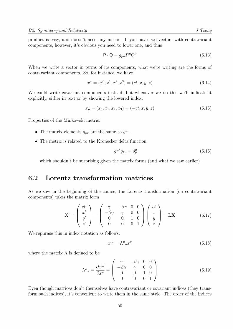
B2: Symmetry and Relativity J Tseng
product is easy, and doesn’t need any metric. If you have two vectors with contravariantcomponents, however, it’s obvious you need to lower one, and thus
P · Q = gµνPµQν (6.13)
When we write a vector in terms of its components, what we’re writing are the forms ofcontravariant components. So, for instance, we have
xµ = (x0, x1, x2, x3) = (ct, x, y, z) (6.14)
We could write covariant components instead, but whenever we do this we’ll indicate itexplicitly, either in text or by showing the lowered index:
xµ = (x0, x1, x2, x3) = (−ct, x, y, z) (6.15)
Properties of the Minkowski metric:
• The matrix elements gµν are the same as gµν .
• The metric is related to the Kronecker delta function
gµλgλν = δµν (6.16)
which shouldn’t be surprising given the matrix forms (and what we saw earlier).
6.2 Lorentz transformation matrices
As we saw in the beginning of the course, the Lorentz transformation (on contravariantcomponents) takes the matrix form
X′ =
ct′
x′
y′
z′
=
γ −βγ 0 0−βγ γ 0 0
0 0 1 00 0 0 1
ctxyz
= LX (6.17)
We rephrase this in index notation as follows:
x′µ = Λµνx
ν (6.18)
where the matrix Λ is defined to be
Λµν =
∂x′µ
∂xν=
γ −βγ 0 0−βγ γ 0 0
0 0 1 00 0 0 1
(6.19)
Even though matrices don’t themselves have contravariant or covariant indices (they trans-form such indices), it’s convenient to write them in the same style. The order of the indices
50

B2: Symmetry and Relativity J Tseng
follows the usual convention, of the row being listed first, whether as an upper or lower index,followed by the column. Indices can be raised and lowered using the metric as with vectors(and tensors).
The covariant transformation must have the form
x′µ = xν(Λ−1)νµ (6.20)
The order of the factors is simply to make the matrix-like multiplication explicit; the factorsthemselves commute, since they just involve numbers. The index order also makes explicitthat
Λµν(Λ
−1)νκ =∂x′µ
∂xν∂xν
∂x′κ= I (6.21)
We can find more about the form of (Λ−1)νκ by combining the two transforms:
x′µ = gµλx′λ (6.22)
= gµλΛλκx
κ (6.23)
= gµλΛλκg
κνxν (6.24)
which leads to the identification
(Λ−1)νµ = gµλΛλκg
κν (6.25)
Indeed, since the g’s raise and lower indices,
(Λ−1)νµ = Λµν (6.26)
This should not be mistaken for a transpose: it is better to consider it a mnemonic remindingyou that you need to use the metric to raise and lower indices to get back to the familiarΛν
µ, with the upper and lower indices in the right order.
In order to see how Λ−1 appears as a matrix, we go back to the more explicit formula
(Λ−1)νκ = gνµgκλΛλµ (6.27)
= gνµ(gκλΛλµ) (6.28)
= gνµ(gΛ)κµ (6.29)
= gνµ(gΛ)Tµκ (6.30)
= (g(gΛ)T )νκ (6.31)
(We have slipped in a matrix transpose, which is safe in this case since the two indices areof one kind.) We then have as a matrix formula
Λ−1 = gΛTg (6.32)
which also implies, since gg = I,ΛT = gΛ−1g (6.33)
Let’s look at the invariance rule again, now in index notation.
gµνAµBν = gµνA
′µB′ν = gµν(ΛµκA
κ)(ΛνλB
λ) = Aκ(ΛµκgµνΛ
νλ)B
λ (6.34)
51

B2: Symmetry and Relativity J Tseng
If we match the components we sum over on the far left and far right sides (µ and ν on theleft, and κ and λ on the right), then we have an equation which looks like a transformationof the metric:
gµν = ΛκµΛλ
νgκλ (6.35)
However, in this case it’s actually a more general way to define the Lorentz transformationΛ, as one which leaves the metric (and therefore any intervals) invariant.
In matrix form, one rewrites the relationship in the form
gµν = ΛκµgκλΛ
λν (6.36)
in order to make the index order match that of matrix multiplication. The first multiplica-tion, however, combines two row indices (the κ index), which implies a multiplication by atransposed matrix:
g = ΛTgΛ (6.37)
which is the familiar result in matrix form.
6.3 Tensors
As we mentioned earlier, scalars are 0-rank tensors, and vectors 1-rank tensors. Scalars areleft unchanged by Lorentz tranformations, while vectors are transformed (contravariantlyor covariantly) by the application of one Λ. Higher rank objects are defined by similartransformation properties. A rank-2 tensor with contravariant components Mµν transformsunder the Lorentz transformation Λ as
M ′µν = ΛµκΛ
νλM
κλ (6.38)
With covariant components,
M ′µν = (Λ−1)κµ(Λ−1)λνMκλ (6.39)
There are also tensors with mixed components:
M ′µν = Λµ
κ(Λ−1)λνM
κλ (6.40)
The order of indices can therefore be important. Individual indices can be raised and loweredusing the metric as with vectors.
Mµν = gνκM
µκ (6.41)
Higher rank tensors can be made from lower-rank objects by taking an “outer” or “tensor”product. For instance, if you have tensors Aµ and Bν , you can form
Cµν = AµBµ (6.42)
This obviously transforms as a rank-2 tensor.
Tensors with rank greater than 2 transform as you’d expect, by piling on more Λ’s in theobvious way. The rank of the tensor is equal to the total number of indices.
52

B2: Symmetry and Relativity J Tseng
The way to reduce the rank of tensors is to contract covariant and contravariant indices.So for instance, if you had a rank-3 tensor Mµν
κ, you can obtain rank-1 tensors Mκνκ and
Mµκκ.
Let’s look again at the invariance of the metric, but this time distinguishing that originalmetric g with one “transformed” along with several vectors.
gµνAµBν = g′µνA
′µB′ν = g′µν(ΛµκA
κ)(ΛνλB
λ) = Aκ(Λµκg′µνΛ
νλ)B
λ (6.43)
To isolate g′µν , we match the elements which multiply particular components of Aµ and Bν ,and then multiply by Λ−1’s (note that the left-multiplication is of the matrix transpose):
Λκµg′κλΛ
λν = gµν (6.44)
Λκµ(Λ−1)µαg
′κλΛ
λν(Λ
−1)νβ = (Λ−1)µαgµν(Λ−1)νβ (6.45)
The multiplication order on the left side looks odd, but remember that we are multiplyingby numbers and the summing over the index µ. We do it in this way in order to reduce thatpart to an identity matrix.
δκαg′κλδ
λβ = (Λ−1)µαgµν(Λ
−1)νβ (6.46)
g′αβ = (Λ−1)µα(Λ−1)νβgµν (6.47)
So we notice that gµν has the transformation rule of two vectors with covariant components(though we know in the end that it’s invariant). In this sense it is properly a rank-2 tensorwith covariant components.
It should be mentioned that the tensors we’ll be using in this course are exclusively Cartesiantensors, with Cartesian coordinates.
It is also worth noting that while we can represent rank-2 tensors with matrices, not allmatrices are rank-2 tensors—even though they look very similar when we write them down,and we use the same index notation and summation convention on both. But they are ratherdifferent objects:
• Matrices such as Λµν represent linear operators, and the principal way to combine
linear operators is to multiply them (though they do form linear spaces in their ownright).
• Tensors represent elements of a linear space. As such, the way to combine tensors isto make linear combinations of them, i.e., with addition and multiplication by scalars.
6.4 *4-gradient
We will see our tensors in differential equations and Euler-Lagrange equations, which meanswe’ll need to take their derivatives. It turns out we can form a vector out of the differentialoperator. Consider the chain rule in light of a coordinate transformation:
∂f
∂x′µ=∂xν
∂x′µ∂f
∂xν(6.48)
53

B2: Symmetry and Relativity J Tseng
When we compare this to the tensor transformation rules, we find that the derivative withrespect to contravariant components acts like a covariant vector. We denote the derivativeas ∂µf .
Similarly, derivatives with respect to covariant components act like a contravariant compo-nent:
∂µ ≡ ∂
∂xµ(6.49)
For convenience, we will still assume non-indexed components are contravariant. So in termsof those usual components,
∂µ ≡∂
∂xµ=
(1
c
∂
∂t,∂
∂x,∂
∂y,∂
∂z
)(6.50)
∂µ ≡ ∂
∂xµ= gµν
∂
∂xν=
(−1
c
∂
∂t,∂
∂x,∂
∂y,∂
∂z
)(6.51)
(6.52)
The d’Alembertian operator is a 4-vector analogue of the ∇2 operator:
22 ≡ ∇2 − 1
c2
∂2
∂t2= ∂µ∂
µ (6.53)
(In some textbooks, and in recent A2 notes, the d’Alembertian is simply 2, but I prefer topreserve the indication of its nature as a second-derivative operator.)
54

Chapter 7
Groups
The reason we’ve gone into all this about tensors is that we want to write down actionswhich respect Lorentz symmetries. This implies that our actions (and Lagrangians) need tobe scalars, i.e., rank-0 tensors.
The main symmetry we’ve looked at is invariance with respect to Lorentz transformations, sothe physics is the same in all inertial frames. Implied in Lorentz invariance is also invariancewith respect to purely spatial rotations. We don’t usually call rotations Lorentz transfor-mations, but as we’ve seen with the Thomas precession, they play a role among Lorentztransformations.
Another symmetry is that of translational invariance, which we’ll touch on later.
In order to understand these symmetries, we’ll draw upon results from a branch of mathe-matics called “group theory”.
A group is a set G and an operator (·) such that
1. Closure: for all a, b ∈ G, then a · b ∈ G as well.
2. Associative property: for all a, b, c ∈ G,
(a · b) · c = a · (b · c)
3. Identity element: there is an element e ∈ G such that a · e = a for all a ∈ G.
4. Inverse element: for each element a ∈ G, there is an element a−1 ∈ G such thata · a−1 = e.
Since this will take a little effort, we’ll start off by spoiling the punchline: a symmetrymeans there are equivalent configurations in a system, and groups allow us mathematicallyto “traverse” this space of equivalent configurations. One of the objectives is to find out whatkinds of physical objects—such as scalars, vectors, and tensors—possess the symmetry, andtherefore can be used to formulate physical laws. In the process, we’ll find that there aremore objects with such symmetry. Some of these are realized in Nature, while others arenot—or, perhaps, just not yet. Symmetry thus becomes one of the guiding principles in theexploration of physics.
55

B2: Symmetry and Relativity J Tseng
7.1 Example: permutation group
Let’s look at a simple example to illustrate how we will use this construct. Consider a systemof three identical bodies placed at the vertices of an equilaterial triangle. Label the bodiesa, b, and c. It is obvious that there are 6 equivalent configurations: abc, bca, cab, acb, cba,and bac.
The configurations themselves don’t form a group. After all, what would be the operation?
Instead, consider the transformations which get you from one configuration to another equiv-alent configuration. Now label the positions 1, 2, and 3. An explicit way to write a trans-formation is, for example, (
1 2 32 3 1
)(7.1)
which means that you take whatever body is in position 1 and move it to position 2, atthe same time moving the body in position 2 to position 3, and the body in position 3 toposition 1. This is, by the way, called a “cyclic permutation”, and the group of operationscalled the “permutation group of degree 3”.
The order of the first row is obviously arbitrary, so we’ll have a conventional order 123.Then we can identify the group elements by the bottom row: 123 (which happens to bethe identity e), 231, 312, 213, 132, and 321. Of course this looks like the configurationsthemselves, because we’ve (arbitrary) chosen one starting point and enumerated the ways toget to all the others.
You can form a multiplication table with these elements, with the first operation on the left,and the second operation listed on the top:
e 231 312 213 132 321e e 231 312 213 132 321
231 231 312 e 321 213 132312 312 e 231 132 321 213213 213 132 321 e 231 312132 132 321 213 312 e 231321 321 213 132 231 312 e
We can see that the group is closed, and that every element has an inverse. It is obviouslynot commutative. (The term for a group with commutative multiplication is “Abelian”; thepermutation group is “non-Abelian”.)
It is also evident that the multiplication results are not randomly scattered everywhere. Forinstance, the elements e, 231, and 312 all multiply amongst themselves; they form a subsetwhich we call a “subgroup”. In fact, they are the cyclic permutations.
Also notice that the other quadrants are also self-contained. This reflects the fact that213, 132, and 321 involve a single swap rather than a cyclic permutation; further cyclicpermutations keep you within the quadrant.
Finally, it is evident you don’t need all the elements in order to traverse the entire groupfrom a single starting point. In fact, all you need is a cyclic permutation p and a swap s.
56

B2: Symmetry and Relativity J Tseng
Then the elements can be written as e, p, pp, s, sp, and spp. Expressions such as ppp andss get you back to e, so pp is clearly the inverse of p, and s is its own inverse.
These sorts of discrete groups are important in physics, and even more so in chemistry whereyou have crystals with these sorts of symmetries. It’s really a couse in itself.
7.2 Rotations
In this course, however, we want to look at systems with continuous symmetries. For in-stance, think of the rotations in 3D of a rigid body like a block of wood with unequal sides.By analogy with the permutation group, choose a starting orientation, and assign to everyorientation a group element which takes you from the starting to final orientation. Thereare clearly an infinite number of group elements, parameterized by continuous parameters.Such a group is commonly called a “Lie group”. In this case there are 3 real parameters.And in fact we’ve seen the infinitesimal rotations already with the generators Ji:
Ri(δθ) = 1− iδθJi (7.2)
From any starting orientation, you can use the three generators to get to any orientation ofthe body itself.
However, as in the case of the permutation group, there is a whole set of configurationswhich cannot be reached. These are the ones which are related to the original orientationby a parity transformation (or spatial inversion, or reflection)
(x, y, z)→ (−x,−y,−z) (7.3)
With an odd number of spatial dimensions, there is no way to get there via infinitesimalrotations.
(In fact it may help to think of a set of vectors, or an extended body, rather than just onevector. The reason is that you can always make a single vector look as if it has gone througha reflection. For instance, you can rotate the vector (1, 1, 1) to get (−1,−1,−1) by rotatingby an angle π around the axis pointing in the (1, 1,−1) direction away from the origin. Whatwon’t be preserved is its relative orientation with respect to another vector.)
At the same time, the reflection clearly leaves all the internal distances within the body thesame. This is an example of a discrete symmetry. So we could include all the orientationsin the group, which we designate O(3), the group of orthogonal transformations in 3D. Atthe same time, it’s clear that if we omit the reflection operation, the remaining operationsform their own group; we call this the “special” subgroup SO(3).
There is a further caveat for 3D rotations: the generators encapsulate how to get from theidentity element to its near neighbors. They don’t necessarily capture global features of thegroup. For instance, there is a redundancy in the rotations, in that a rotation by π around anaxis n is equivalent to a rotation by π around the opposite axis −n. The group is consideredconnected, but not simply connected. In fact, it’s doubly connected: one can visualize theissue by considering three parameters, the direction of n being specified by angles θ ∈ [0, π]
57

B2: Symmetry and Relativity J Tseng
and φ ∈ [0, 2π], and the rotation angle by ψ ∈ [0, 2π]. The space of rotations can be thoughtof as a solid sphere with radius π, with n the direction relative to the origin, and ψ thedistance from the origin. The non-simple connection arises from the fact that points on thesurface of the sphere are equivalent to opposite points on the surface.
Again, as in the case of the permutation group, we need to keep in mind that the group isthat of rotations, not of configurations. This is implied in the use of generators: you rotatea little bit from orientation A to B, and then a little more from B to C. If you started fromanother orientation, you could go through the same set of rotations, but it would take youthrough a different series of orientations.
7.3 Representations
A group is an abstract concept, and don’t have to refer to any specific physical entities.On the other hand, to handle group elements, and especially to do any calculations, weoften need to play with concrete mathematical objects which must therefore have the sameproperties as the group.
For instance, the group of rotations can be represented by a group of rotation matrices whichoperate on 3-vectors. The two groups have exactly the same behavior, in that the matrixwhich is the product of two rotation matrices itself represents the resulting rotation. Thisis an example of an isomorphism, in which the elements of two groups G and H have aone-to-one correspondence, and that g1g2 = g3 in for elements in G is true if and only ifh1h2 = h3 for the corresponding elements in H.
A homomorphism is a slightly looser construction: it preserves the multiplication rule, butloses the requirement that there be a one-to-one correspondence. Representations of groupsare often homomorphic (rather than isomorphic) to the original group.
Physicists often don’t make strong distinctions between abstract groups and their represen-tations. Unfortunately, we also sometimes forget the distinction between the group repre-sentations (i.e., the operators) and the objects on which they operate. Within the group,the rotation operators act not on vectors (which aren’t members of the group, after all) buton other rotation operators. And indeed the rotations may not work on vectors, but otherobjects, which we’ll explore in a little while. We’ll try to refer to the space of objects asthe “representation space” of the representation. The group analysis is independent of thoseconcrete objects which lie outside the group.
7.3.1 Orthogonal matrices
To return to the rotation example, we can associate members of the 3D rotation group withthe set of 3× 3 orthogonal matrices, which have the property that
RTR = I (7.4)
A possible representation space is then the linear space of 3D vectors.
58

B2: Symmetry and Relativity J Tseng
This also enables us to appreciate the relationship between rotations and spatial inversion.If we take the determinant of both sides of the above equation, we find that
(det R)2 = 1 (7.5)
det R = ±1 (7.6)
A normal rotation has det R = +1, but a reflection has det R = −1. Since all the infinites-imal rotations also have det R = +1, and the determinant of a product of two matrices issimply the product of the two determinants, it’s obvious you can’t get to a transformationwith det R = −1.
Now let’s look at the generators. You’ve already seen something very much like them inquantum mechanics when dealing with angular momentum. In particular, they do notcommute, and the relations are familiar:
[Ja,Jb] ≡ JaJb − JbJa = iεabcJc (7.7)
This is sometimes called the “Lie algebra”, and it determines the local behavior of thegroup—in other words, if you have one element, what is the relationship between the nearbyelements? Since the continuous symmetries are based on infinitesimal transformations, itshouldn’t be surprising that the Lie algebra determines most of the most important propertiesof the group.
We can derive representations of the SO(3) group by considering its Lie algebra. We definethe operators
J2 = J21 + J2
2 + J23 (7.8)
J± = J1 ± iJ2 (7.9)
The algebra is familiar from quantum mechanics: these are just linear operators, so it’s allthe same as before, but we recap here. The key observation, however, is that all this followsfrom the Lie algebra, the knowledge that the generators are Hermitian (which is true forrotations, but not for boosts), and that there is a finite basis set.
The first operator commutes with all the Ja. For instance, consider its commutator with J1:
[J2,J1] = [J22,J1] + [J2
3,J1] (7.10)
= J2[J2,J1] + [J2,J1]J2 + J3[J3,J1] + [J3,J1]J3 (7.11)
= −iJ2J3 − iJ3J2 + iJ2J3 + iJ3J2 (7.12)
= 0 (7.13)
We call such operators “Casimir operators”.
The other two operators are raising and lowering operators. By making them out of J1 andJ2, we’ve chosen to use the eigenvectors of J3 as the basis. Therefore
J3|m〉 = m|m〉 (7.14)
59

B2: Symmetry and Relativity J Tseng
We calculate the following commutators:
[J3,J±] = [J3,J1]± i[J3,J2] (7.15)
= iJ2 ∓ i2J1 (7.16)
= iJ2 ± J1 (7.17)
= ±J± (7.18)
This allows us to see the effect of the operators on the eigenvectors:
J3J+|m〉 − J+J3|m〉 = [J3,J+]|m〉 = J+|m〉 (7.19)
J3J+|m〉 = (m+ 1)J+|m〉 (7.20)
J3J−|m〉 − J−J3|m〉 = [J3,J−]|m〉 = −J−|m〉 (7.21)
J3J−|m〉 = (m− 1)J−|m〉 (7.22)
So we find thatJ±|m〉 ∝ |m± 1〉 (7.23)
Since the basis is finite, there must be both a maximum and minimum m value. Themaximum mmax is defined with
J3|mmax〉 = mmax|mmax〉 (7.24)
J+|mmax〉 = 0 (7.25)
To evaluate the J2 eigenvalue, we first note that
J+J− = (J1 + iJ2)(J1 − iJ2) (7.26)
= J21 + J2
2 + i[J2,J1] (7.27)
= J2 − J23 + J3 (7.28)
and similarlyJ−J+ = J2 − J2
3 − J3 (7.29)
Then we have
J2|mmax〉 = (J23 + J3 + J−J+)|mmax〉 (7.30)
= (m2max +mmax + 0)|mmax〉 (7.31)
= mmax(mmax + 1)|mmax〉 (7.32)
From this maximum m, we traverse backwards using successive applications of J−, steppingby −1 each time. We can show that the J2 eigenvalue applies to all the other eigenvectors,since J2 commutes with all the Ja, and therefore all powers of J−:
J2Jn−|mmax〉 = Jn−J2|mmax〉 (7.33)
= mmax(mmax + 1)Jn−|mmax〉 (7.34)
Since we’ve now shown the role of mmax, we can revert to the familiar terminology and callit j.
60

B2: Symmetry and Relativity J Tseng
If we take all the |m〉 to be properly normalized, then we can find the coefficients left by theJ± operators:
〈m|J†+J+|m〉 = 〈m|J−J+|m〉 = 〈m|(J2 − J23 − J3)|m〉 = j(j + 1)−m(m+ 1) (7.35)
〈m|J†−J−|m〉 = 〈m|J+J−|m〉 = 〈m|(J2 − J23 + J3)|m〉 = j(j + 1)−m(m− 1) (7.36)
and therefore, summarizing,
J±|m〉 = [j(j + 1)−m(m± 1)]1/2|m± 1〉 (7.37)
At the minimum m value, we have
J3|mmin〉 = mmin|mmin〉 (7.38)
J−|mmin〉 = 0 (7.39)
0 = 〈mmin|J†−J−|mmin〉 (7.40)
= 〈mmin|J+J−|mmin〉 (7.41)
= 〈mmin|(J2 − J23 + J3)|mmin〉 (7.42)
= j(j + 1)−mmin(mmin − 1) (7.43)
If we take all the |m〉 to be properly normalized, then we find that mmin = −j. For the seriesto be finite, j must be either an integer or half-integer.
So we get a set of eigenvectors (members of the representation space) with the eigenvalues jand m where
J2|jm〉 = j(j + 1)|jm〉 (7.44)
J3|jm〉 = m|jm〉 (7.45)
J± |jm〉 =√j(j + 1)−m(m± 1)|j,m± 1〉 (7.46)
j = 0,1
2, 1,
3
2, 2, · · · (7.47)
m = −j,−j + 1, · · · , j − 1, j (7.48)
This looks like quantum mechanics, but we’re still dealing with classical physics. The im-portant thing to remember here is that whatever happens to your physical intuition withquantum mechanics, it doesn’t modify mathematics. (Another way of saying this is that theorigin of this algebra is not quantum mechanical, but geometrical.)
The representations are characterized by the eigenvalue j, with the corresponding 2j + 1eigenvectors spanning the representation space. Obviously most of these representations arehomomorphic to the rotation group, rather than isomorphic. The simplest (trivial) exampleis j = 0, which maps all the rotations onto the identity element. The generators in this case(and in this representation basis, not the Cartesian basis we started with) are Jk = 0 for allk, so they trivially satisfy the Lie algebra. Only the j = 1 representation is isomorphic tothe rotation group itself.
We can check that the j = 1 representation behaves as we expect. To do so, we should beexplicit about bases, because we’ve actually given the generators in two.
61

B2: Symmetry and Relativity J Tseng
First, we used the Cartesian basis, which is convenient for its geometric roots. In this basis,
J3 =
0 −i 0i 0 00 0 0
(7.49)
and the rotation matrix is
R3(α) = e−iαJ3 =
cosα − sinα 0sinα cosα 0
0 0 1
(7.50)
In the “canonical” basis of the j = 1 representation, the corresponding generator is
J3 =
1 0 00 0 00 0 −1
(7.51)
so for a finite rotation this becomes
R3 = e−iαJ3 = 1− i sinαJ3 + (cosα− 1)J23 (7.52)
Since we can see that J23 is “almost” an identity,
J23 =
1 0 00 0 00 0 1
(7.53)
we can write down the rotation matrix directly:
R3 =
1− i sinα + cosα− 1 0 00 1 00 0 1 + i sinα + cosα− 1
=
e−iα 0 00 1 00 0 eiα
(7.54)
Is this really a rotation matrix around the z axis? Let’s examine how the matrix affects anappropriate representation space, such as the l = 1 spherical harmonics.
Y ′11(θ, φ) = Y1
1(θ, φ)eiα =1
2
√3
2πsin θe−i(φ−α) (7.55)
Y ′10(θ, φ) = Y1
0(θ, φ) =1
2
√3
πcos θ (7.56)
Y ′1−1
(θ, φ) = Y1−1(θ, φ)e−iα = −1
2
√3
2πsin θei(φ−α) (7.57)
(7.58)
Since the xy dependence in these spherical harmonics is in the φ exponential, it appears therotation matrix has rotated the basis functions by a consistent angle α.
62

B2: Symmetry and Relativity J Tseng
7.3.2 Spinor representation
What of the j = 1/2 representation? This has 2 basis vectors with m = ±1/2, which wedesignate |+〉 and |−〉. Following the same procedure as before, we make J3 out of theeigenvalues:
J3 =1
2
(1 00 −1
)(7.59)
The action of the raising and lower operators is
J+|−〉 = |+〉 (7.60)
J−|+〉 = |−〉 (7.61)
so the operators are
J+ =
(0 10 0
)(7.62)
J− =
(0 01 0
)(7.63)
(7.64)
which allow us to write down J1 and J2:
J1 =1
2(J+ + J−) =
1
2
(0 11 0
)(7.65)
J2 = − i2
(J+ − J−) =1
2
(0 −ii 0
)(7.66)
In short,
Ji =σi2
(7.67)
where σi are the Pauli matrices.
A finite rotation around the z axis is
eiθJ3 = 1− iθJ3 −θ2
2!J2
3 + iθ3
3!J3
3 + · · · (7.68)
= 1− iθ2σ3 −
θ2
222!σ2
3 + iθ3
233!σ3
3 + · · · (7.69)
= cosθ
2− iσ3 sin
θ
2(7.70)
taking advantage of the fact that σ2j = I. In this case, we see that it takes a rotation through
4π to get back to the identity. A full rotation through 2π, on the other hand, gets you to−1.
It is worth pausing to consider what these results mean. The Pauli matrices are themselves abasis set for traceless, Hermitian 2× 2 matrices, and the exponential of these matrices yield2 × 2 unitary matrices. In fact, they yield a subset of unitary matrices we denote SU(2):
63

B2: Symmetry and Relativity J Tseng
the group of unitary matrices with determinant 1. This group has the same Lie algebra asSO(3); after all, that’s how we got it in the first place. This means that the local behaviorof moving from one element of its representation space to another is identical to that of 3Drotations.
Moreover, SU(2) is simply connected, unlike SO(3). The easiest way to see this is to considera general element of SU(2) in the form
U =
(a− ib −c− id−c+ id a+ ib
)(7.71)
where a, b, c, and d are real parameters. One can verify that it’s unitary
U†U =
(a+ ib c+ id−c+ id a− ib
)(a− ib −c− id−c+ id a+ ib
)(7.72)
=
(a2 + b2 + c2 + d2 0
0 a2 + b2 + c2 + d2
)(7.73)
=
(1 00 1
)(7.74)
with the constraint thatdet U = a2 + b2 + c2 + d2 = 1 (7.75)
The group manifold is therefore a unit (Euclidean) 4-sphere, with no equivalent points.Because SU(2) is simply connected, any element can be written uniquely as an exponentialof generators. It is actually a “covering group” of SO(3), with identical local behavior but“unrolling” the latter’s double connection into the double cover.
7.3.3 Spinor representation space
(Based on Steane’s chapter on spinors)
Now, we might ask, what is the representation space of the j = 1/2 representation? In thiscase, we only have a representation in the canonical basis, whereas for j = 1 we had bothcanonical and and convenient Cartesian bases, the latter of which provided a more readyintuition as to what was going on.
On the other hand, we should have some sense of a rotation, so we expect that there canbe some relationship with Cartesian components. Indeed, since we expect the 2-dimensionalrepresentation space to have complex coefficients, we certainly have enough degrees of free-dom to represent a 3-vector—and more.
We can write the spinors in terms of 4 real parameters r, θ, φ, and α. The first 3 parametersdefine a usual 3-vector in polar coordinates. The last parameter then encodes an additionalorientation, like a little flag flying from a 3-vector flagpole. The actual definition of theorientation doesn’t mean much at this point, because the rotations of SO(3) don’t affect it.
The 2-component spinor is then
s =
(ab
)= se−iα/2
(cos θ
2e−iφ/2
sin θ2eiφ/2
)(7.76)
64
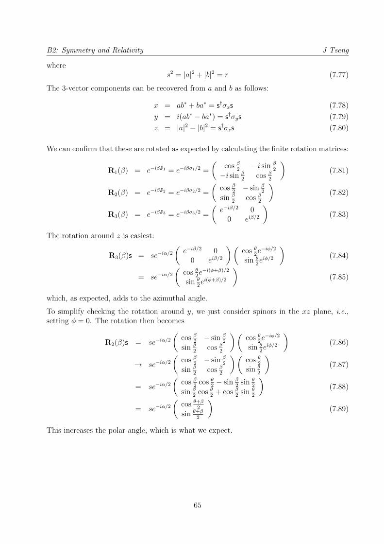
B2: Symmetry and Relativity J Tseng
wheres2 = |a|2 + |b|2 = r (7.77)
The 3-vector components can be recovered from a and b as follows:
x = ab∗ + ba∗ = s†σxs (7.78)
y = i(ab∗ − ba∗) = s†σys (7.79)
z = |a|2 − |b|2 = s†σzs (7.80)
We can confirm that these are rotated as expected by calculating the finite rotation matrices:
R1(β) = e−iβJ1 = e−iβσ1/2 =
(cos β
2−i sin β
2
−i sin β2
cos β2
)(7.81)
R2(β) = e−iβJ2 = e−iβσ2/2 =
(cos β
2− sin β
2
sin β2
cos β2
)(7.82)
R3(β) = e−iβJ3 = e−iβσ3/2 =
(e−iβ/2 0
0 eiβ/2
)(7.83)
The rotation around z is easiest:
R3(β)s = se−iα/2(e−iβ/2 0
0 eiβ/2
)(cos θ
2e−iφ/2
sin θ2eiφ/2
)(7.84)
= se−iα/2(
cos θ2e−i(φ+β)/2
sin θ2ei(φ+β)/2
)(7.85)
which, as expected, adds to the azimuthal angle.
To simplify checking the rotation around y, we just consider spinors in the xz plane, i.e.,setting φ = 0. The rotation then becomes
R2(β)s = se−iα/2(
cos β2− sin β
2
sin β2
cos β2
)(cos θ
2e−iφ/2
sin θ2eiφ/2
)(7.86)
→ se−iα/2(
cos β2− sin β
2
sin β2
cos β2
)(cos θ
2
sin θ2
)(7.87)
= se−iα/2(
cos β2
cos θ2− sin β
2sin θ
2
sin β2
cos θ2
+ cos β2
sin θ2
)(7.88)
= se−iα/2(
cos θ+β2
sin θ+β2
)(7.89)
This increases the polar angle, which is what we expect.
65

B2: Symmetry and Relativity J Tseng
For rotating around x, we check at φ = π/2, i.e., in the yz plane.
R1(β)s = se−iα/2(
cos β2−i sin β
2
−i sin β2
cos β2
)(cos θ
2e−iφ/2
sin θ2eiφ/2
)(7.90)
→ se−iα/2√2
(cos β
2−i sin β
2
−i sin β2
cos β2
)((1− i) cos θ
2
(1 + i) sin θ2
)(7.91)
=se−iα/2√
2
((1− i) cos β
2cos θ
2− (1 + i)i sin β
2sin θ
2
−i(1− i) sin β2
cos θ2
+ (1 + i) cos β2
sin θ2
)(7.92)
=se−iα/2√
2
((cos β
2cos θ
2+ sin β
2sin θ
2) + i(− cos β
2cos θ
2− sin β
2sin θ
2)
(− sin β2
cos θ2
+ cos β2
sin θ2) + i(− sin β
2cos θ
2+ cos β
2sin θ
2)
)(7.93)
=se−iα/2√
2
((1− i) cos θ−β
2
(1 + i) sin θ−β2
)(7.94)
= se−iα/2(e−iπ/4 cos θ−β
2
eiπ/4 sin θ−β2
)(7.95)
In this case, the rotation is in the opposite sense of increasing the polar angle, so β issubtracted from θ.
7.3.4 Spinor representation with matrices
There is actually no particular reason the representation space has go be built out of columnvectors. The requirement is that the space has to be linear, and that one can obtain a scalar(the norm) out of it.
In fact, it’s (arguably) easier to represent spinors with 2×2 matrices. Associate each 3-vectorx with a 2× 2 unitary matrix as follows:
X = xiσi =
(z x− iy
x+ iy −z
)(7.96)
The norm of the object is
|X| = − det X = −z2 − (x+ iy)(x− iy) = −x2 − y2 − z2 (7.97)
Now, with each transformation U, associate the similarity transformation:
X′ = UXU† (7.98)
Since U ∈ SU(2), the determinant of U is +1. We then have the relationship
det X′ = det X (7.99)
so the norm is clearly preserved by the transformation.
As a side note (which is actually rather important from other perspectives), we also see Uand −U results in the same transformation. This is another manifestation of the doublecover of SU(2) over SO(3).
66

B2: Symmetry and Relativity J Tseng
Let’s try out a rotation:
R3(β)XR†3(β) =
(e−iβ/2 0
0 eiβ/2
)(z x− iy
x+ iy −z
)(eiβ/2 0
0 e−iβ/2
)(7.100)
=
(ze−iβ/2 (x− iy)e−iβ/2
(x+ iy)eiβ/2 −zeiβ/2)(
eiβ/2 00 e−iβ/2
)(7.101)
=
(z (x− iy)e−iβ
(x+ iy)eiβ −z
)(7.102)
so we can see that z is unaffected, and the angle of (x + iy) has been increased by β. Onecan test the other rotations as well.
Is there a relationship between these two spaces? We can form a 2 × 2 matrix from thecolumn spinors by taking the outer product:
2ss† = 2s2
(cos θ
2e−iφ/2
sin θ2eiφ/2
)(cos θ
2eiφ/2 sin θ
2e−iφ/2
)(7.103)
= 2r
(cos2 θ
2sin θ
2cos θ
2e−iφ
sin θ2
cos θ2eiφ sin2 θ
2
)(7.104)
= r
(1 + cos θ sin θe−iφ
sin θeiφ 1− cos θ
)(7.105)
from which we see thatX = 2ss† − r1 (7.106)
The transformation then follows:
X′ = UXU† (7.107)
= 2Uss†U† − rUU† (7.108)
= 2s′s′† − r1 (7.109)
We can then see that the transformation of X is closely related to the transformation of s.
7.3.5 Higher-spin representations
Representations with higher j values can be obtained through the same algebra, but theycan also be obtained by combining lower-j representations. You’re already familiar with theprocedure from quantum mechanics, where it was called “addition of angular momenta.”
As an example, you can take a direct product of two j = 1/2 representations. Elements ofthe direct product representation space have the form of the tensor product
ξaζb (7.110)
where a and b are indices taking on values 1 or 2. The space is designated 12⊗ 1
2.
The direct product space can be broken up into subspaces with different j values (in groupterminology, we are reducing the space into its irreducible representations, which are the
67

B2: Symmetry and Relativity J Tseng
representations with a well-defined j). As expected, you get a j = 0 space and a j = 1 space.The j = 0 space transforms as a scalar, while the j = 1 space, with its 3 basis elements,transforms as a 3-vector. The matrix operators in the new basis are then block diagonal,with operators for the different j subspaces in each block. This combined representation iscalled a direct sum representation, and in this case is written 0⊕1. In fact, you have alreadyseen something like this in action, in the relationship between the two spinor representationspaces; some authors make the analogy that a spinor is a sort of “square root” of a vector.
68
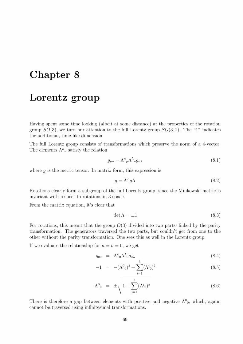
Chapter 8
Lorentz group
Having spent some time looking (albeit at some distance) at the properties of the rotationgroup SO(3), we turn our attention to the full Lorentz group SO(3, 1). The “1” indicatesthe additional, time-like dimension.
The full Lorentz group consists of transformations which preserve the norm of a 4-vector.The elements Λµ
ν satisfy the relation
gµν = ΛκµΛλ
νgκλ (8.1)
where g is the metric tensor. In matrix form, this expression is
g = ΛTgΛ (8.2)
Rotations clearly form a subgroup of the full Lorentz group, since the Minkowski metric isinvariant with respect to rotations in 3-space.
From the matrix equation, it’s clear that
det Λ = ±1 (8.3)
For rotations, this meant that the group O(3) divided into two parts, linked by the paritytransformation. The generators traversed the two parts, but couldn’t get from one to theother without the parity transformation. One sees this as well in the Lorentz group.
If we evaluate the relationship for µ = ν = 0, we get
g00 = Λκ0Λλ
0gκλ (8.4)
−1 = −(Λ00)2 +
3∑i=1
(Λi0)2 (8.5)
Λ00 = ±
√√√√1 +3∑i=1
(Λi0)2 (8.6)
There is therefore a gap between elements with positive and negative Λ00, which, again,
cannot be traversed using infinitesimal transformations.
69

B2: Symmetry and Relativity J Tseng
There are therefore 4 divisions of the full Lorentz group. Of these, we’ll be concerned withthe division which forms a subgroup, i.e., contains the identity element. This is called the“orthochronous” (preserving the normal time direction) Lorentz group:
det Λ = +1 (8.7)
Λ00 ≥ 1 (8.8)
The subgroup is denoted SO(3, 1)↑+, where the superscript indicates it’s the orthochronousdivision, and the subscript the parity. Since we’ll pretty much just talk about this subgroup,we’ll drop the decorations and call it SO(3, 1) by default; if we need another division, we’llmention it specifically.
8.1 Commutators
As with SO(3), we start by looking at the Lie algebra, which tells us about the local behaviorof the group’s transformations. The commutators are
[Ja,Jb] = iεabcJc (8.9)
[Ka,Jb] = iεabcKc (8.10)
[Ka,Kb] = −iεabcJc (8.11)
The first commutator is simply the one for rotations. The third commutator shows that thedifference in the order of two non-aligned Lorentz boosts is a rotation. We’ve already seenthe physical effect of this non-zero commutator. (It’s worth noting that since two non-alignedboosts aren’t in general equivalent to a single boost, but a boost and a rotation, boosts don’tby themselves form a group.)
The Lie algebra is already suggestive of rotations. It can be made even more suggestive bycombining the operators:
Ma = (Ja + iKa)/2 (8.12)
Na = (Ja − iKa)/2 (8.13)
The commutators then become
[Ma,Mb] = iεabcMc (8.14)
[Na,Nb] = iεabcNc (8.15)
[Ma,Nb] = 0 (8.16)
So we now have two, disjoint SU(2) algebras. We can think of this as the direct productSU(2)× SU(2).
We saw before that SU(2) was the cover group for SO(3), in that it preserved the localrelationships between the infinitesimal transformations, but had better global properties inthat its group manifold was simply connected. Similarly, there is a (double) cover group forthe Lorentz group, the “special linear group” SL(2,C) of 2 × 2 matrices with determinant
70

B2: Symmetry and Relativity J Tseng
+1. The group SU(2) is obviously a subgroup of SL(2,C), and indeed SL(2,C) is the“complexified” direct product SU(2) × SU(2). And as with SU(2) compared with SO(3),it has the same local behavior but also better global behavior, i.e., it is simply connected,unlike SO(3, 1).
The direct product structure allows us to enumerate the representations. Two Casimiroperators immediately suggest themselves: M2, with eigenvalues m(m + 1), and N2, witheigenvalues n(n + 1). Both m and n are nonnegative integers or half-integers. So we writedown the pair (m,n).
8.2 Fundamental representations
The structure SU(2)×SU(2) suggests looking at spin-1/2 representations. Let’s start as wehad with the rotation group, with one addition:
X = xµσµ =
(ct+ z x− iyx+ iy ct− z
)(8.17)
The components can be extracted using the trace
xµ =1
2tr(Xσµ) (8.18)
The Lorentz transformation then takes the form
X′ = AXA† (8.19)
where A ∈ SL(2,C) is the matrix corresponding to the Lorentz transformation of xµ. Anelegant way of summarizing this is that
A(xµσµ)A† = (Λxµ)σµ (8.20)
We’d like to write the vector as a direct product of spinors, X = ξξ†. This tells us that theappropriate Lorentz transformation matrix is A, since
X′ = AXA† = Aξξ†A† = (Aξ)(Aξ)† = ξ′ξ′† (8.21)
So a Lorentz transform Λ on a vector corresponds with the matrix A on a spinor.
This seems simple enough, but if you look in different texts on the subject, you’ll see differentconventions at work. The main difference is which transformation is taken as a starting pointfor deriving all the other transformation rules. We’ll use a convention which has become fairlyconventional in the larger physics community. Toward that end, we define
ψa → ψ′a = Aabψb (8.22)
ψa → ψ′a
= ψb(A−1)ba
(8.23)
Notice that in this convention, it is the covariant spinor which transforms with the matrix A,and the contravariant spinor with its inverse. In the end, all these differences reflect manip-ulations of some initial matrix; once the initial matrix is defined for a given transformation,the other forms follow.
71

B2: Symmetry and Relativity J Tseng
First, let’s find an invariant tensor that performs as a metric. It turns out that we can usethe asymmetric tensor εab:
εab =
(0 1−1 0
)(8.24)
The tensor ε plays a similar role to the metric g, though there are some subtleties abouthow it raises and lowers indices because it is, unlike g, antisymmetric:
εab = −εab (8.25)
and as result,εabψb 6= ψbε
ba (8.26)
A common convention is that ε raises/lowers from the left:
ψa = εabψb (8.27)
ψa = εabψb (8.28)
For matrix indices,εabAb
cεcd = Aad (8.29)
So if you write down matrix elements in one form, with indices in one configuration (such asAb
c), but then need to use the matrix with indices in another configuration (such as Abc),you will need to use ε’s to raise and lower to get the form you need.
In that spirit, the elements of the matrix form of εcd are defined by
εabεbc = εac = δac (8.30)
as appropriate for a metric-like tensor, so
εab =
(0 −11 0
)(8.31)
The two tensors clearly act as inverses of one another.
We now have two ways of writing the transformation of ψa. The first is the definition itself,in terms of A−1. The second is to use ε to relate it to the covariant transformation:
ψ′a
= εabψ′b (8.32)
= εabAbcψc (8.33)
= εabAbcεcdψ
d (8.34)
Comparison with the contravariant transformation rules yields
(A−1)ba
= εacAcdεdb (8.35)
Since this is in the form of a similarity transformation SAS−1, it is clear the covariant andcontravariant spinor representations are equivalent.
72

B2: Symmetry and Relativity J Tseng
Now let’s see what happens when we take the complex conjugate of these transformations.We define
χa = (χa)∗ (8.36)
χa = (χa)∗ (8.37)
where we’ve dotted the indices to anticipate that we’ll need to account for them separatelyfrom undotted ones. The transformation of the conjugate contravariant spinor follows:
χ′a
= (χ′a)∗ (8.38)
= (χb(A−1)ba)∗ (8.39)
= (χb)∗((A−1)ba)∗ (8.40)
In order to simplify the matrix part, we start from equivalence we found above:
(A−1)ba
= εacAcdεdb = Aab (8.41)
((A−1)ba)∗ = (Aad)
∗ = (A∗)ab (8.42)
So we can now write the conjugate contravariant spinor transformation as
χ′a
= (A∗)abχb (8.43)
We then transform the conjugate covariant spinor:
χ′a = (χ′a)∗ (8.44)
= (Aabχb)
∗ (8.45)
= (Aab)∗χb (8.46)
To find the matrix elements, we use the equivalence again:
(A−1)ba
= εacAcdεdb (8.47)
((A−1)ba)∗ = εac(Ac
d)∗εdb (8.48)
εma(A∗−1)b
aεbn = εmaε
ac(Acd)∗εdbε
bn (8.49)
εnb(A∗−1)baεma = (A∗)m
n (8.50)
(A∗−1)nm = (A∗)mn (8.51)
We have used the matrix form of ε liberally to evaluate its transpose and complex conjugate.The last relationship can be written in matrix notation as
A∗−1 = A† (8.52)
and the conjugate covariant spinor transformation is
χ′a = χb(A∗−1)ba (8.53)
73

B2: Symmetry and Relativity J Tseng
In summary,
ψa → ψ′a = Aabψb (8.54)
ψa → ψ′a
= ψb(A−1)ba
(8.55)
χa → (A∗)abχb (8.56)
χa → χb(A∗−1)ba (8.57)
As we saw earlier, the first two of these transformation rules are equivalent, as are the lasttwo. But it turns out that the first two are not equivalent with the latter two.
To see that, let’s write down expressions for A. We use the same rotation generators asbefore:
Ja =1
2σa (8.58)
For boosts, we can write down
Ka =i
2σa (8.59)
It is straightforward to verify that this works for boosts in the z direction.
A = eησ3/2 = coshη
2+ σ3 sinh
η
2=
(eη/2 0
0 e−η/2
)(8.60)
Then we have A† = A, and
X′ = AXA† (8.61)
=
(eη/2 0
0 e−η/2
)(ct+ z x− iyx+ iy ct− z
)(eη/2 0
0 e−η/2
)(8.62)
=
((ct+ z)eη/2 (x− iy)eη/2
(x+ iy)e−η/2 (ct− z)e−η/2
)(eη/2 0
0 e−η/2
)(8.63)
=
((ct+ z)eη x− iyx+ iy (ct− z)e−η
)(8.64)
(8.65)
The transformed coordinates can be evaluated using the trace:
ct′ =1
2trX′ =
1
2(ct(eη + e−η) + z(eη − e−η)) = ct cosh η + z sinh η (8.66)
z′ =1
2tr(X′σ3) =
1
2(ct(eη − e−η) + z(eη + e−η)) = ct sinh η + z cosh η (8.67)
It is straightforward but tedious to verify this in boosts in the other directions. With thesegenerators, a general transformation matrix can be written in the form
Aab = e−i(θkJk+ηkK) (8.68)
= e−i2
(θkσk+iηkσk) (8.69)
= e−12
(iθk−ηk)σk (8.70)
74

B2: Symmetry and Relativity J Tseng
Now let’s take the complex conjugate.
(A∗)ab = εac(A∗)cdεdb (8.71)
where we’ve used the ε matrices to put the indices in the right place so we can use theexpression we found for the Aa
b matrix elements.
(A∗)cd = e−
12
(−iθk−ηk)σ∗k (8.72)
When we evaluate the exponential, we can insert ε−1ε in between all the σ∗k matrices. Wecan evaluate these quickly:
εσ∗1ε−1 =
(0 1−1 0
)(0 11 0
)(0 −11 0
)(8.73)
=
(1 00 −1
)(0 −11 0
)(8.74)
=
(0 −1−1 0
)= −σ1 (8.75)
εσ∗2ε−1 =
(0 1−1 0
)(0 i−i 0
)(0 −11 0
)(8.76)
=
(−i 00 −i
)(0 −11 0
)(8.77)
=
(0 i−i 0
)= −σ2 (8.78)
εσ∗3ε−1 =
(0 1−1 0
)(1 00 −1
)(0 −11 0
)(8.79)
=
(0 −1−1 0
)(0 −11 0
)(8.80)
=
(−1 00 1
)= −σ3 (8.81)
so in generalεσ∗kε
−1 = −σk (8.82)
and we find(A∗)ab = εac(A∗)c
dεdb = e−12
(iθk+ηk)σ∗k (8.83)
We see then that using ε to transform A acts in different ways on rotations on boosts, asseen in the different signs in the exponent. This is an indication of the inequivalency betweenthese two representations.
Since the sign of the boost is the difference, we can simply flip its sign for the conjugaterepresentation:
Ka = − i2σa (8.84)
75
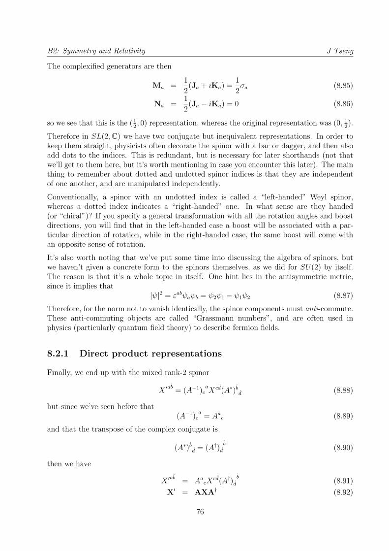
B2: Symmetry and Relativity J Tseng
The complexified generators are then
Ma =1
2(Ja + iKa) =
1
2σa (8.85)
Na =1
2(Ja − iKa) = 0 (8.86)
so we see that this is the (12, 0) representation, whereas the original representation was (0, 1
2).
Therefore in SL(2,C) we have two conjugate but inequivalent representations. In order tokeep them straight, physicists often decorate the spinor with a bar or dagger, and then alsoadd dots to the indices. This is redundant, but is necessary for later shorthands (not thatwe’ll get to them here, but it’s worth mentioning in case you encounter this later). The mainthing to remember about dotted and undotted spinor indices is that they are independentof one another, and are manipulated independently.
Conventionally, a spinor with an undotted index is called a “left-handed” Weyl spinor,whereas a dotted index indicates a “right-handed” one. In what sense are they handed(or “chiral”)? If you specify a general transformation with all the rotation angles and boostdirections, you will find that in the left-handed case a boost will be associated with a par-ticular direction of rotation, while in the right-handed case, the same boost will come withan opposite sense of rotation.
It’s also worth noting that we’ve put some time into discussing the algebra of spinors, butwe haven’t given a concrete form to the spinors themselves, as we did for SU(2) by itself.The reason is that it’s a whole topic in itself. One hint lies in the antisymmetric metric,since it implies that
|ψ|2 = εabψaψb = ψ2ψ1 − ψ1ψ2 (8.87)
Therefore, for the norm not to vanish identically, the spinor components must anti-commute.These anti-commuting objects are called “Grassmann numbers”, and are often used inphysics (particularly quantum field theory) to describe fermion fields.
8.2.1 Direct product representations
Finally, we end up with the mixed rank-2 spinor
X ′ab
= (A−1)caXcd(A∗)bd (8.88)
but since we’ve seen before that(A−1)c
a= Aac (8.89)
and that the transpose of the complex conjugate is
(A∗)bd = (A†)db
(8.90)
then we have
X ′ab
= AacXcd(A†)d
b(8.91)
X′ = AXA† (8.92)
76

B2: Symmetry and Relativity J Tseng
which is what we started with. Xab is a member of the (12, 1
2) representation. Since the pair
of numbers expresses a direct product, we expect that, for instance, (12, 1
2) can be reduced to
a direct sum in the usual way1
2⊗ 1
2= 0⊕ 1 (8.93)
In fact, we can get all the other (m,n) representations by taking direct products of (0, 12)
and (12, 0).
8.3 Space inversion
Earlier, we talked of the parity transformation (or spatial inversion) as inaccessible to ro-tations in three dimensions. However, we know that most physics is invariant even underthis transformation, so we’d like to enlarge our group to include this transformation as well.This would mean adding SO(3, 1)↑− to the SO(3, 1)↑+ we’ve been considering so far. We’lljust denote this in the utterly expected way, as SO(3, 1)↑.
That said, we know that some physics actually does look different on spatial inversion. Thisphenomenon is called “parity violation”, and is associated in paricular with the electroweakinteraction in particle physics. For now, however, we’ll take parity as a further symmetry.
The parity operator can be written in matrix form
P =
1 0 0 00 −1 0 00 0 −1 00 0 0 −1
(8.94)
It is easy to see that this operator commutes with spatial rotations:
PRP−1 = R (8.95)
which can be checked in matrix form, or by visualizing it.
For Lorentz transformations, we see, for example,
PL1P−1 =
1 0 0 00 −1 0 00 0 −1 00 0 0 −1
cosh η sinh η 0 0sinh η cosh η 0 0
0 0 1 00 0 0 1
1 0 0 00 −1 0 00 0 −1 00 0 0 −1
(8.96)
=
cosh η − sinh η 0 0− sinh η cosh η 0 0
0 0 1 00 0 0 1
(8.97)
In general,PL(η)P−1 = L(−η) = L−1(η) (8.98)
which makes sense, that 3-vectors should flip sign under spatial inversion.
77

B2: Symmetry and Relativity J Tseng
In terms of generators,
PJiP−1 = Ji (8.99)
PKiP−1 = −Ki (8.100)
We can follow these into the complexified generators:
PMjP−1 = P
(Jj + iKj
2
)P−1 =
Jj − iKj
2= Nj (8.101)
PNjP−1 = P
(Jj − iKj
2
)P−1 =
Jj + iKj
2= Mj (8.102)
and thus, for the Casimir operators,
PM2P−1 = N2 (8.103)
PN2P−1 = M2 (8.104)
What this means is that the two parts of the direct product SU(2) × SU(2) are no longercompletely factorized when considering spatial inversion as well. P connects them. As aresult, a representation (u, v) becomes (v, u) under spatial inversion.
Since we expect physical objects to be in some representation space of SO(3, 1)↑ (except forthose cases where experiment has demonstrated otherwise!), we expect them to come in twoclasses: a direct sum of two representations (u, v)⊕ (v, u), with u 6= v; and a self-conjugaterepresentation, with u = v.
In the latter case, spatial inversion acts on the basis vectors (labelled by the eigenvalues mu
and mv)P |mumv〉 = η|mvmu〉 (8.105)
If we also demand that P 2 = 1, then we find that η = ±1. (In fact, with spinors it’s alsopossible to use P 2 = −1, analogous to a rotation R(2π) = −1.)
Scalars belong to the (0, 0) representation space. If η = 1, then we have the normal scalarswhich are invariant under Lorentz transformations as well as spatial inversion. If η = −1,then it’s still invariant under Lorentz transformations, but changes sign under spatial inver-sion; this is called a “pseudo-scalar”.
4-vectors belong to the (12, 1
2) space, as we saw earlier. Here again we have two cases: η = 1,
which in this case means the sign changes under spatial inversion (“polar vectors”); andη = −1, in which case the sign doesn’t change (“axial vectors”). Spacetime displacements,momentum, and vector potentials are polar vectors. We’ll see examples of axial vectors later,though it’s worth noting that a 3D version of an axial vector is the magnetic field.
78

Chapter 9
Poincare group
So far, we’ve focused on rotations and boosts, but of course spacetime has translationalsymmetry, in that translations also keep the relativistic interval invariant. When we extendthe symmetry group to include translations, we get the Poincare group, which is sometimescalled the “inhomogeneous Lorentz group”.
We won’t work out all the details, because what we’re really aiming to do is to describe therepresentations.
A translation can be writtenxµ → x′
µ= xµ + aµ (9.1)
If we have a function of the spacetime event, we expand it to find the effect of an infinitesimaltranslation aµ as follows:
f(x′µ) = f(xµ) +
∂f
∂xµaµ (9.2)
We compare this with the generator definition
T (aµ) = 1 + iaµPµ (9.3)
which gives us the generatorsPµ = −i∂µ (9.4)
These obviously commute amongst themselves. They’re often designated the linear momen-tum operators.
Similarly, the angular momentum operators generate rotations; in Minkowski space, we alsotake in boosts. The spatial part of angular momentum can be written in differential form:
Lµν ≡ xµPν − xνPµ = −i(xµ∂ν − xν∂µ) (9.5)
79

B2: Symmetry and Relativity J Tseng
The commutator with the linear momentum operator is
[Lµν , Pρ] = [−i(xµ∂ν − xν∂µ),−i∂ρ] (9.6)
= −[xµ∂ν , ∂ρ] + [xν∂µ, ∂ρ] (9.7)
= −xµ∂ν∂ρ + ∂ρ(xµ∂ν) + xν∂µ∂ρ − ∂ρ(xν∂µ) (9.8)
= (∂ρgµλxλ)∂ν − (∂ρgνλx
λ)∂µ (9.9)
= gµλδλρ∂ν − gνλδλρ∂µ (9.10)
= gµρ∂ν − gνρ∂µ (9.11)
= i(gµρ(−i∂ν)− gνρ(−i∂µ)) (9.12)
= i(gµρPν − gνρPµ) (9.13)
Similarly, one can evaluate the commutators amongst the L’s. The commutators are then
[Pµ, Pν ] = 0 (9.14)
[Lµν , Pρ] = i(gµρPν − gνρPµ) (9.15)
[Lµν , Lκλ] = i(Lµλgνκ + Lνκgµλ − Lµκgνλ − Lνλgµκ) (9.16)
Now, L is not the most general form of an angular momentum operator you can write. Youcan also add a term
Jµν = Lµν + Sµν (9.17)
as long as the Sµν commutes with the Lµν , and has all the same commutation relations—in other words, acts just like another angular momentum. We can then summarize thecommutation relations with this generalized angular momentum instead:
[Pµ, Pν ] = 0 (9.18)
[Jµν , Pρ] = i(gµρPν − gνρPµ) (9.19)
[Jµν , Jκλ] = i(Jµλgνκ + Jνκgµλ − Jµκgνλ − Jνλgµκ) (9.20)
In matrix form, the Jµν operators can be written in a fairly easy-to-remember antisymmetricform
(Jµν)ρσ = i(δρµδ
σν − δσµδρν) (9.21)
Note, however, that the matrix indices are both raised. To get this into the form with whichwe do matrix multiplication, we take
(Jµν)ρσ = gσλ(Jµν)
ρλ (9.22)
= igσλ(δρµδ
λν − δλµδρν) (9.23)
= i(δρµgσν − δρνgσµ) (9.24)
The familiar generators are then
Ji =1
2εijkJjk (9.25)
Ki = J0i (9.26)
One can confirm this results in the usual matrix generators.
80

B2: Symmetry and Relativity J Tseng
9.1 Casimir operators
There are two Casimir operators. The most obvious is PµPµ. Since the eigenvalues of P µ
are the momenta components pµ, the eigenvalues of PµPµ are pµp
µ.
The second Casimir operator is a generalization of angular momentum, but now folded inwith momentum. Its role is played by what is called the “Pauli-Lubanski” vector
W µ ≡ 1
2εµνκλPνJκλ (9.27)
where εµνκλ is the 4-index Levi-Civita symbol. We’ve written this with the generalizedangular momentum, but it is useful to break this up into orbital and internal (spin) angularmomentum parts. The orbital angular momentum has the form
Lκλ = xκPλ − xλPκ (9.28)
so the orbital part of the Pauli-Lubanski vector is
W µ =1
2εµνκλPν(xκPλ − xλPκ) (9.29)
=1
2εµνκλ(xκPνPλ − xλPνPκ) (9.30)
= −1
2εµκνλ(xκPνPλ − xλPνPκ) (9.31)
(the last step is simply to put the ν index next to κ and λ so it’s only one index swap away).Since the P ’s commute, but ε is completely antisymmetric, each term sums to zero.
The same argument doesn’t apply to the spin angular momentum. Instead, it is useful toevaluate the vector by component. First, we remind ourselves that we can get the spacecomponents of the spin vector from the definitions we used before:
Si =1
2εijkSjk (9.32)
and S0 = 0. The Pauli-Lubanski components are then
W 0 =1
2ε0ijkPiSjk (9.33)
= PiSi (9.34)
= p · s (9.35)
W i =1
2εiνκλPνSκλ (9.36)
=1
2εi0κλP0Sκλ (9.37)
= −1
2ε0ijkP0Sjk (9.38)
= −P0Si (9.39)
= (E/c)s (9.40)
81

B2: Symmetry and Relativity J Tseng
(keeping in mind that P0 is the covariant component of the usual 4-momentum). In summary,the orbital angular momentum parts have dropped out and we are left with
W = (p · s, (E/c)s) (9.41)
The properties of W µ are as follows:
W µPµ = 0 (9.42)
[W µ, P µ] = 0 (9.43)
[W λ, Jµν ] = i(W νgλµ −W µgνλ) (9.44)
[W µ,W ν ] = iεµνκλWκPλ (9.45)
The Casimir operator is W µWµ.
9.2 Representation space of the Poincare group
The representation space of the Poincare group now brings us back to physical particles, theinhabitants of the representation space of the symmetry groups we’ve been discussing.
The representations of the Poincare group can be used to classify particles and fields (V Bargman,EP Wigner, Proc Natl Ac Sci, 34:5, 211 (1946)). The unitary representations are as follows:
1. P µPµ = −m2 where m is a real number. These are finite-mass particles, with spinvalues s = 0, 1
2, 1, 3
2, etc. The eigenvalue of W µWµ is m2s(s + 1). States are labelled
by the spin z-component s3 and the (continuous) 3-momentum p.
2. P µPµ = 0 and W µWµ = 0. We can write these 4-vectors as
P = (|p|,p) (9.46)
W = (w0,w) (9.47)
with the 0th component of W
(w0)2 = w ·w (9.48)
w0 = ±√|w| (9.49)
However, we also have
0 = P ·W (9.50)
= −w0|p|+ p ·w (9.51)
w0|p| = |p||w| cos θ (9.52)
where θ is the angle between w and p. Clearly cos θ = ±1, so w and p are eitherparallel or anti-parallel.
82

B2: Symmetry and Relativity J Tseng
The constant of proportionality between these vectors is the “helicity”
λ =w0
p0=
s · p|p|
= ±s (9.53)
since s is proportional to w, which is parallel or anti-parallel to p. Therefore masslessparticles with non-zero spin have two helicities: photons with s = ±1, gravitons withs = ±2, and (in the massless approximation) neutrinos with s = ±1
2.
3. P µPµ = 0 but W µWµ > 0. These are massless particles but with continuous spin.Particles of this type have not been found.
4. P µPµ > 0. Particles in this category would be tachyons. Only found in two circum-stances: science fiction, or virtual contributions to (non-fiction) scattering amplitudes.
9.2.1 Supersymmetry and spacetime
The Poincare algebra is complete in itself: its generators all commute among one anotherand to no other generators.
The Coleman-Mandula theorem states that one cannot introduce any further generators intothis algebra. In other words, if there are further symmetries, they can only be internal sym-metries, and their Lie algebra will not involve non-trivial commutators with the generatorsof translations, rotations, and boosts. The linear space over which the generators operate isadded to spacetime as a direct product.
The essence of proof is (apparently) fairly simple: in a hypothetical scattering experimentin which the input 4-momenta of 2 particles are known, the final state is known up to thescattering angle—in classical mechanics, this scattering angle is determined by the impactparameter, which of course is not specified among the 4-momenta. On the other hand, ifthere are further symmetries, then the final state would lose this degree of freedom, andwould either be completely determined or overconstrained. (If you want to look it up, itmay be worth reading later versions of the proof, for instance by Witten or Weinberg, ratherthan the original.)
However, there is a loophole in the theorem: it only applies to vectorial degrees of freedom.Spinors are not similarly constrained. As a result, spinorial operators can be added to thePoincare algebra. This extension is called “supersymmetry”. In quantum field theory, thisresults in certain famous results, among them the idea that for every fundamental fermionthere must be a bosonic “superpartner”. In a sense, supersymmetry is an extension ofspacetime symmetries, and it’s such a compelling idea that twenty years ago, some seniortheoretical physicists expressed concern that there might be theory postgraduates out therewho didn’t realize it was an unproven idea.
Twenty years later, it remains unproven, so the role it might play in physics is so far undeter-mined. Its relevant energy scale is so far anywhere between whatever current experimentalbounds exist, and the unification of gravity with all the other forces. Experimentally, themost obvious manifestation of supersymmetry is the flagrant overuse of the prefix “super”.
83

B2: Symmetry and Relativity J Tseng
9.3 Physics tensors
Let’s continue to look at members of the representation space of our symmetry groups. Thereare not just particles, but also fields which transform as tensors.
9.3.1 3D tensors
We have already seen one rank-2 tensor, albeit as an operator: (spacetime) angular momen-tum.
Lµν = xµpν − xνpµ (9.54)
It’s worth taking a moment to look at 3D tensors in connection with angular momentum.There is the angular momentum tensor itself
Lij = xipj − xjpi (9.55)
as well as the momentum of inertia tensor.
Iij =
∫V
dm(r2δij − rirj) (9.56)
Since we’re dealing with the spatial dimensions, the symmetry group we’re talking about isSO(3) of rotations. Therefore the rotation takes the form
L′ij = RimRjnLmn (9.57)
in which we recognize the matrix equation
L′ = RLRT (9.58)
Moreover, since R is orthogonal, RT = R−1, so the transformation is the same as a similaritytransform. In other words, you may have seen this rotation as a basis change for a matrix.Equivalently (for 3D), it’s a legitimate tensor transformation.
9.3.2 *Transformation of electromagnetic fields
Now let’s take a peek at electromagnetism. We have two fields, E and B. How do theytransform between frames?
One approach is to look at how the force transforms. After all, it’s the force, rather thefields, which you “see” by their effect on other particles. We will see that the fields don’tlook like Lorentz 4-vectors.
The force per unit charge isf = q(E + v ∧B) (9.59)
Notice that for f to be a normal polar vector which changes sign under spatial inversion, weneed E to also be a polar vector. The cross product then means that B has to be an axialvector which doesn’t change sign under spatial inversion.
84

B2: Symmetry and Relativity J Tseng
The first scenario to consider: a single test charge q in a constant electric field E but withB = 0. The test charge has a velocity u in frame S. The force in the test charge is thus
f = qE (9.60)
Now let’s transform into the frame S ′ which travels with velocity v in S. We know that theforce should transform as follows:
f ′‖ =f‖ −
(vc2
)dEdt
1− u·vc2
(9.61)
f ′⊥ =f⊥
γv(1− u·v
c2
) (9.62)
For a pure force (when the rest mass stays constant, so the force goes into the kinetic energyof the particle), we have
0 = U · F = (γuc, γuu) ·(γuc
dE
dt, γuf
)= γ2
u
(−dEdt
+ u · f)
(9.63)
so we see thatdE
dt= f · u (9.64)
Plugging this into the formula for f‖, we get
f ′‖ =f‖ − v(f · u)/c2
1− u · v/c2(9.65)
If we choose v = u such that the test particle is at rest in S ′, we have
f‖ = qE‖ (9.66)
f · u = qE · u (9.67)
f ′‖ =q(E‖ − v(E · u)/c2)
1− u · v/c2(9.68)
=q(E‖ − E‖β
2)
1− β2(9.69)
= qE‖ (9.70)
f ′⊥ =qE⊥
γ(1− β2)(9.71)
= γqE⊥ (9.72)
from which we infer that
E′‖ = E‖ (9.73)
E′⊥ = γE⊥ (9.74)
It is clear that E‖ doesn’t transform at all like a 4-vector, which would boost the longitudinalcomponent, and leave the transverse part alone.
85

B2: Symmetry and Relativity J Tseng
And indeed there is also a magnetic field in S ′, though for the v = u case, the resulting forceis zero, since the test charge is at rest. To see some effect, keep v parallel to u, but nowv 6= u. The velocity of the test charge in S ′ is now u′, which must still be parallel to v. Butsince the force in S ′ must be of the form
f ′ = q(E′ + u′ ∧B′) (9.75)
we will only pick out the component of B′ which is perpendicular to v.
Using the transformation formula for the transverse force,
f ′⊥ =f⊥
γv(1− u · v/c2)(9.76)
=qE⊥
γv(1− u · v/c2)(9.77)
We’d like to write this in terms of quantities in S ′. The denominator can be changed byconsidering the velocity addition formula:
u′‖ =u‖ − v
1− u · v/c2(9.78)
u′‖ · v =u‖ · v − v2
1− u · v/c2(9.79)
1 + u′‖ · v/c2 =1− u · v/c2 + u · v/c2 − v2/c2
1− u · v/c2(9.80)
=1− v2/c2
1− u · v/c2(9.81)
γ2v(1 + u′‖ · v/c2) =
1
1− u · v/c2(9.82)
so plugging in,f ′⊥ = qE⊥γv(1 + u′‖ · v/c2) (9.83)
Comparing this with the force equation, we see that
u′ ∧B′ = E⊥γvu′v/c2 (9.84)
This is consistent with a perpendicular magnetic field component
B′⊥ = −γ(v ∧ E)/c2 (9.85)
In any case, it’s clear that the Lorentz transformation is mixing up electric and magneticfields.
9.3.3 *The Maxwell field tensor
What is happening? It turns out that E and B aren’t parts of independent 4-vectors, butrather of a single tensor, which we can write
F µν ≡
0 Ex/c Ey/c Ez/c
−Ex/c 0 Bz −By
−Ey/c −Bz 0 Bx
−Ez/c By −Bx 0
(9.86)
86

B2: Symmetry and Relativity J Tseng
This is the “Maxwell field tensor”. In terms of Lorentz group representation, it belongs to(0, 1)⊕ (1, 0), which brings out the involvement of two types of 3-vectors.
A Lorentz transformation takes the form
F ′µν
= ΛµκΛ
νλF
κλ (9.87)
or in matrix form (suppressing c for now)
F′ = ΛFΛT (9.88)
=
γ −βγ 0 0−βγ γ 0 0
0 0 1 00 0 0 1
0 Ex Ey Ez−Ex 0 Bz −By
−Ey −Bz 0 Bx
−Ez By −Bx 0
γ −βγ 0 0−βγ γ 0 0
0 0 1 00 0 0 1
(9.89)
=
γ −βγ 0 0−βγ γ 0 0
0 0 1 00 0 0 1
−βγEx γEx Ey Ez−γEx βγEx Bz −By
−γEy + βγBz βγEy − γBz 0 Bx
−γEz − βγBy βγEz + γBy −Bx 0
(9.90)
=
0 γ2Ex − β2γ2Ex γEy − βγBz γEz + βγBy
β2γ2Ex − γ2Ex 0 −βγEy + γBz −βγEz − γBy
−γEy + βγBz βγEy − γBz 0 Bx
−γEz − βγBy βγEz + γBy −Bx 0
(9.91)
which results in the following transformed fields:
E ′x = Ex (9.92)
E ′y = γ(Ey − βBz) (9.93)
E ′z = γ(Ez + βBy) (9.94)
B′x = Bx (9.95)
B′y = γ(By + βEz) (9.96)
B′z = γ(Bz − βEy) (9.97)
If we rotate our transformation to another axis, we get the following more general forms:
E‖ → E‖ (9.98)
E⊥ → γ(E⊥ + v ∧B) (9.99)
B‖ → B‖ (9.100)
B⊥ → γ(B⊥ − v ∧ E) (9.101)
(9.102)
87

Chapter 10
Classical fields
We’ve now looked at what kinds of objects transform, and how they transform. In theprocess we found that there are some additional objects which obey the transformation, i.e.,are consistent with Special Relativity. Now we’ll look at how we join these things togetherin equations of motion.
The main lesson: Lagrangians are functionals which can be made to result in a scalar. Theyhave to be scalars in order for the search for an extremal path to have a meaning; if theyweren’t, there would be no ordering and therefore no extreme value. And because the scalaris invariant with respect to Lorentz transformations, we’ll find that the extremal path is alsoinvariant.
This isn’t quite as possible with Hamiltonians, since in many cases Hamiltonians are acomponent of a 4-vector.
We have taken the symmetries of Special Relativity as the focus of our study, but it’snot the only possible set of symmetries. In fact, an important avenue for research is tounderstand other symmetries we observe, sometimes only indirectly, and sometimes only inapproximation. In order to incorporate them, however, we need to find an action which hasboth old and new symmetries. So finding “new physics” is a matter of elucidating the formof the action. Symmetries guide and constrain the form of such actions.
10.1 The field viewpoint
In previous lectures, we’ve seen how a Lagrangian can be written to yield results consis-tent with Special Relativity. Those Lagrangians were limited to the behavior of individualparticles in some external potential which was not itself form-invariant. This is of some-what limited applicability. What we’d like to do is write Lagrangians which are entirelyform-invariant, including all the interactions.
The interactions present a particular problem, since in Special Relativity the interactionsthemselves have a propagation speed. But there is a way to do this, by folding those interac-tions into a continous field. The interactions then propagate as field changes: an interactioncan start in one location, find its way to another, and then cause its effect.
88

B2: Symmetry and Relativity J Tseng
This then raises the other main motivation for a field viewpoint: locality. With the fieldviewpoint, we have been able to phrase all known laws of Nature as local interactions, i.e.,interactions happen where things overlap in spacetime. We have thus been able to eliminatenotions of action at a distance, which was a rather unsatisfactory model even as Newtonproposed it for gravity.
10.2 Continuous systems
(Based on Goldstein chapter 12)
Let’s take an example of a discrete system from which we can extract a continuous limit: aline of coupled uniform harmonic oscillators.
The non-relativistic Lagrangian:
T =1
2
∑i
mη2i (10.1)
V =1
2
∑i
k(ηi+1 − ηi)2 (10.2)
L = T − V (10.3)
=1
2
∑i
(mη2i − k(ηi+1 − ηi)2) (10.4)
where ηi are the displacements of the ith particles from their equilibrium positions.
Introduce the parameter a, the equilibrium separation between masses:
L =1
2
∑i
a
(m
aηi − ka
(ηi+1 − ηi
a
)2)
=∑i
aLi (10.5)
So in the limit of infinitesimal a, we have m/a → µ, the mass density, and ka → Y , theYoung’s modulus (extension per unit length of an elastic rod, which is proportional to theforce exerted on the rod). Then we take the sum into an integral
L =1
2
∫ (µ
(∂η
∂t
)2
− Y(∂η
∂x
)2)dx (10.6)
where now η ≡ η(x, t). Note that now that η is a function of both x and t, we need to useexplicit partial derivatives.
The most important point here is that the position coordinate x is no longer one of thegeneralized coordinates of a path. Instead, it serves as a label: it replaces the label i. So xbecomes like t in its status in the Lagrangian. Likewise, the generalized coordinates are nowη and its derivatives with respect to x and t.
89

B2: Symmetry and Relativity J Tseng
10.3 Lagrangian density
Now let’s look at this more generically.
The Lagrangian we want would integrate the field over all the space “labels”:
L =
∫d3xL(η, ∂µη, x
µ) (10.7)
where
∂µη ≡∂η
∂xµ(10.8)
is a shorthand for a particular kind of partial derivative where you differentiate with re-spect to one “label” coordinate (such as x or t) while holding the other “label” coordinatesconstants. This isn’t much of an issue for a field η, which here is only a function of thoselabel-type coordinates. However, L is a function of the fields, the field derivatives, and thecoordinates. So
∂µL =∂
∂xµL(η(xν), ∂µη(xν), xν) (10.9)
will be interpreted as the partial derivative of L considering it as a function of the “label”coordinates. In other words, it differentiates through the fields via the chain rule. This hasrather clumsily been called a “total partial derivative”.
The action to minimize is then
I[η(xµ)] =
∫Ldt =
∫∫V
d4xL(η, ∂µη, xµ) (10.10)
L is technically the “Lagrangian density”, but it’s often called the “Lagrangian” anyway,the distinction usually being clear in context. The spacetime volume V is such that the fieldvalues of η are fixed on its boundaries.
As we noted before, the action isn’t a property of a particle or a field: its only job is to givethe equations of motion via the Euler-Lagrange equations. There are therefore any numberof possible actions to describe some given physics. On the other hand, experience has givenus some guidelines as to some reasonable constraints (Ramond, p 24):
1. the fields in the Lagrangian depend only on one spacetime point, i.e., we consideronly “local” field theories. Indeed, we use local field theories to describe non-localphenomena as well.
2. the action I is real-valued. Complex-valued actions—specifically, potentials—tend toresult in matter disappearing, which isn’t very satisfying classical physics (at least).
3. the Lagrangian depends on no higher than second derivatives. Higher-order differentialequations tend to lead to non-causal solutions. The implication is that Lagrangianstend to have products of first derivatives, which result in second-order derivatives inthe equations of motion.
90

B2: Symmetry and Relativity J Tseng
4. the action reflects other symmetries. For instance, most of the actions and Lagrangianswe’ll see in this course are relativistically invariant, i.e., they are scalars. But theremay be further symmetries with respect to other degrees of freedom, such as electriccharge. In quantum field theories, there will be further internal degrees of freedom,such as the phase of the quantum field at a given spacetime point.
Let’s illustrate evaluating the stationary field configuration for one field η(x, t) in x and t.
L ≡ L(η, ∂xη, ∂tη, x, t) (10.11)
The variation is then
0 = δI = δ
∫dxdtL (10.12)
It should be noted that the variation changes the field and its derivative, not x and t, whichare just labels for the field values. In a sense, the extension of classical field theory tospecial relativity is actually rather simple, since the Lorentz transformation only affects thelabels. As long as the quantities which make up L transform appropriately, you can get awaywithout worrying too much about Special Relativity itself—except for a subtle point aboutintegration limits.
Since we know the fields at the x and t boundary, we take the variation to be zero at theboundary. Let
η(x, t;α) = η(x, t; 0) + αζ(x, t) (10.13)
where η(x, t; 0) is the correct function which satisfies Hamilton’s Principle, and ζ(x, t) is anywell-behaved (continuous) function which vanishes at the boundary.
Take the derivative of the integral
0 =dI
dα=
∫dxdt
dLdα
(10.14)
=
∫dxdt
(∂L∂η
∂η
∂α+
∂L∂(∂tη)
∂(∂tη)
∂α+
∂L∂(∂xη)
∂(∂xη)
∂α
)(10.15)
=
∫dxdt
(∂L∂η
ζ +∂L
∂(∂tη)
∂ζ
∂t+
∂L∂(∂xη)
∂ζ
∂x
)(10.16)
At this point most texts refer blithely to “integrating by parts”, but let’s be a bit moreexplicit here because it’ll help us understand the nature of derivatives we take.
In multivariable calculus, integrating by parts is essentially an application of Stokes’ Theo-rem (or its specialization or generalization, depending on the number of dimensions you’reworking in). In this case we’re specializing to two dimensions, so we’ll use Stokes’ Theoremin x and y (to keep our minds on the geometric nature of this integral):∫
S
∇∧ F · da =
∮C
F · ds (10.17)
we get for a field F = (P,Q, 0), where P and Q are both functions of x and y,∫S
(∂Q
∂x− ∂P
∂y
)dxdy =
∮C
(Pdx+Qdy) (10.18)
91

B2: Symmetry and Relativity J Tseng
Now let’s go back into x−−t space by changing y to t, and then substituting
P = − ∂L∂(∂tη)
ζ (10.19)
Q =∂L
∂(∂xη)ζ (10.20)
Now we need to careful with derivatives here. As far as Stokes’ Theorem is concerned, Pand Q are functions only of x and t (or y), but L is a function of η and its derivatives aswell. So when we take the derivative of Q with respect to x, we actually need to carry thederivative through η and its derivatives (like a full derivative), while keeping t constant (likea partial derivative). In other words, the derivative we need is the “total partial derivative”we described earlier.
∂Q
∂x→ ∂xQ =
∂Q
∂x+∂Q
∂η
∂η
∂x+
∂Q
∂(∂xη)
∂(∂xη)
∂x+
∂Q
∂(∂tη)
∂(∂tη)
∂x(10.21)
So we end up with∫S
(∂xQ− ∂tP )dxdt =
∫S
(∂x
(∂L
∂(∂xη)
)ζ +
∂L∂(∂xη)
∂ζ
∂x+ ∂t
(∂L
∂(∂tη)
)ζ +
∂L∂(∂tη)
∂ζ
∂t
)dxdt
(10.22)and ∮
C
(Pdx+Qdt) =
∮C
ζ
(− ∂L∂(∂tη)
dx+∂L
∂(∂xη)dt
)(10.23)
which is zero because ζ = 0 on the boundary.
Thus we end up with
0 =
∫dxdt
[∂L∂η− ∂t
(∂L
∂(∂tη)
)− ∂x
(∂L
∂(∂xη)
)]ζ (10.24)
In this case it doesn’t help to “choose” ζ to be zero anywhere, because the integral isthroughout the spacetime volume of paths.
But since the path variation ζ is arbitrary, the square bracketed part must vanish.
So in general, for each field φk,
0 = ∂µ
(∂L
∂(∂µφk)
)− ∂L∂φk
(10.25)
These are the Euler-Lagrange equations for fields.
It is also worth reminding oneself that the derivative with respect to a contravariant co-ordinate/label xµ is covariant, and the derivative of L with respect to the (covariant) fieldderivative is contravariant. Thus the sum in the first term is a simple sum—no metric needed.
In summary, the Lagrangian approach for fields is very similar to those for particles, butwith coordinates qi and qi replaced with an infinite number of values indexed by space-time
92

B2: Symmetry and Relativity J Tseng
position.
i → xµ, k (10.26)
qi → φk(x) (10.27)
qi → ∂µφk(x) (10.28)
L =∑i
Li(qi, qi) →∫L(φk, ∂µφk)d
3x (10.29)
Finally, in order to guarantee Lorentz form-invariance, L has to be a scalar: it has to beconstructed from elements of the representation space for the Poincare symmetry group.
93

Chapter 11
Relativistic field equations
Now we’ll take a look at some relativistic field equations.
11.1 *Classical Klein-Gordon equation
The simplest field should be that of the (0, 0) representation, which is just a scalar fieldφ(xµ). We can also form vectors out of the derivatives ∂µφ, though these would have to becontracted to give a scalar in the Lagrangian.
If we also want to have a linear equation of motion, we can only involve up to quadraticterms in φ and ∂µφ. So this suggests a Lagrangian
L = −1
2(∂µφ)(∂µφ)− 1
2m2φ2 (11.1)
where the signs and factors anticipate later interpretation. Note that the mass-like factor mhere has units of L−1, but we keep it this way for simplicity; in normal units (reintroducingc and ~, the factor would be mc/~.
Since we know how to differentiate ∂µφ, rather than the contravariant version, we rewritethe Lagrangian with the metric
L = −1
2gµν(∂µφ)(∂νφ)− 1
2m2φ2 (11.2)
The derivatives are then
∂L∂φ
= −m2φ (11.3)
∂L∂(∂µφ)
= −gµν∂νφ (11.4)
The “total partial derivatives” will be simple, since the second formula above only involves∂φ/∂xµ. So the total partial derivative is the same as the partial derivative with respect tospacetime labels. The Euler-Lagrange equation is then
0 = −∂µ∂µφ+m2φ (11.5)
94

B2: Symmetry and Relativity J Tseng
This is the Klein-Gordon equation for a single scalar field.
There are two ways to look at interpreting this equation. On the one hand, we can compareit with the Lagrangian density of the coupled harmonic oscillators,
L =1
2µ(∂tφ)2 − 1
2Y (∂xφ)2 (11.6)
in which we see something like the derivative term. The speed of a propagating wave mustbe something like Y/µ.
For the second term of the Klein-Gordon equation, an interpretation is suggested when wereplace the partial derivatives with momentum operators
0 = (−i∂µ)(−i∂µ)φ+m2φ = (PµPµ +m2)φ (11.7)
which looks like the “on-shell” condition of a particle with mass m. This is even more explicitwhen we plug in “free particle” solutions
φ = Ae−ikµxµ
(11.8)
which results in the equation0 = kµk
µ +m2 (11.9)
Classically, this is a travelling wave with an effective mass, i.e., a certain resistance to changesin inertia.
Another type of solution can be found by postulating a spherical solution, such as one mighthave for emissions from a point source. It’s instructive to look at the time-independent case:
∇2φ(x) = m2φ(x) (11.10)
which we turn into a radial equation
1
r
∂2
∂r2(rφ(r)) = m2φ(r) (11.11)
∂2
∂r2(rφ(r)) = m2(rφ(r)) (11.12)
(11.13)
We postulate the form of the solution to be
rφ(r) = Ae−mr +Bemr (11.14)
Since we are interested in the source solution, we take B = 0, and we end up with
φ(r) = Ae−mr
r(11.15)
If this was a photon with m = 0, this looks like the Coulomb field. And indeed, if you wantto add a Coulomb interaction to a Lagrangian, you add to it the product of the two fields:the field (or particle), and the Coulomb field.
95

B2: Symmetry and Relativity J Tseng
If m 6= 0, then we have a field which is exponentially suppressed, with length scale m−1: it’sas if the non-zero mass limits the range of the interaction. This idea lies behind the Yukawaexplanation of the short-range forces which keep the nucleus together. Since the nuclearlength scale is on the order of 10−15 m, we get a mass on the order of a hundred or so MeV.
The pion, which was discovered soon afterwards, has a mass a little under 140 MeV. However,a cautionary tale: it wasn’t the first. The muon (mass 105 MeV) was discovered first, andwas hailed as the Yukawa meson. The problem was that it had none of the properties ofa force-carrying particle: it was a fermion, and, worse yet, it didn’t interact much withnucleons. In some older textbooks (not just those published before the π was discovered),the muon is still referred to as a µ-meson. The lesson is that one really has to check theproperties of new particles, not just their masses. There is still a lot of work to do, forinstance, in measuring the properties of the Higgs boson.
11.1.1 Complex-valued fields
If the field is complex-valued, we can describe two fields in a single Lagrangian.
L = −1
2(∂µφ
∗)(∂µφ)− 1
2m2φ∗φ (11.16)
It turns out that we can treat a field and its complex conjugate as two independent fields.But how should we differentiate with respect to φ and φ∗? One way to see how to do this isto separate the two into independent real components:
φ = u+ iv (11.17)
Then if we have a function f(φ, φ∗) to extremize,
0 = δf =∂f
∂φ(δu+ iδv) +
∂f
∂φ∗(δu− iδv) (11.18)
from which we conclude (since δu and δv are arbitrary),
0 =∂f
∂φ+
∂f
∂φ∗
0 =∂f
∂φ− ∂f
∂φ∗
or, equivalently,
0 =∂f
∂φ
0 =∂f
∂φ∗
96

B2: Symmetry and Relativity J Tseng
Therefore we can proceed to differentiate with respect to φ and φ∗ as if they were independent.The derivatives are then
∂L∂φ
= −1
2m2φ∗ (11.19)
∂L∂(∂µφ)
= −1
2gµν∂νφ
∗ (11.20)
∂L∂φ∗
= −1
2m2φ (11.21)
∂L∂(∂µφ∗)
= −1
2gµν∂νφ (11.22)
and the Euler-Lagrange equations
0 = ∂µ
(∂L
∂(∂µφ)
)− ∂L∂φ
(11.23)
0 = −1
2gµν∂µ∂νφ
∗ +1
2m2φ∗ (11.24)
0 = −∂µ∂µφ∗ +m2φ∗ (11.25)
Similarly,0 = −∂µ∂µφ+m2φ (11.26)
Thus we have two independent fields satisfying the same equation of motion and with thesame mass.
11.2 Dirac equation
The next “simplest” (or at least next most fundamental) field should involve the members ofthe (1
2, 0)⊕ (0, 1
2) representation. Their equation of motion is known as the Dirac equaiton.
What will be done here is in all likelihood profoundly unhistorical: Dirac was trying to figureout how to get rid of the second derivative in time implied by the Klein-Gordon equation,and when he found that he couldn’t solve his new equation with single-valued functions, hepostulated multi-valued functions—often written as 4-component column matrices—whichwere found to correspond to spin-1/2 particles.
Approaching from group theoretical considerations, one immediately “sees” a 4-componentrepresentation, because we have the direct sum of two 2-component spinors from the conju-gate (and inequivalent) representations. In the Weyl (chiral) basis, we write a Dirac spinoras
ψ =
(ψLψR
)=
(φχ
)=
φ1
φ2
χ1
χ2
(11.27)
where we need to keep in mind that the φ, χ, ψL, and ψR are 2-component spinors. In the firstversion, we broke up ψ into left-handed and right-handed components. These correspond tothe undotted and dotted spinors we see on the right side.
97

B2: Symmetry and Relativity J Tseng
Then it’s a matter of coming up with a suitable equation of motion which is first-order intime. We have the vector ∂µφ, but contracting it with itself will result in a second-orderequation. Instead, we need to look at how to construct invariants with Dirac spinors. Ifwe only had rotations to deal with, then a spinor η† · η would be fine, but it would not beinvariant with respect to the parity transformation. Instead, we form the linear combination
(χ)† · φ+ χ · φ† (11.28)
or, to make the left and right-handed explicit,
ψ†L · ψR + ψ·Lψ†R (11.29)
To write this in matrix form with the Dirac spinor itself, we define the matrix
γ0 =
(0 II 0
)(11.30)
and thus the invariant scalar is
ψ†γ0ψ = ψ†L · ψR + ψ†R · ψL (11.31)
This will work for the mass term in the Lagrangian.
Notational caution: the adjoint of the Dirac spinor is also often designated with a bar
ψ ≡ ψ†γ0 (11.32)
The reason it’s useful here is that when we take derivatives of the Lagrangian, we’ll takederivatives with respect to ψ and its (Dirac) adjoint ψ. For this course, we’ll just have toput up with this a short while.
For the kinetic term (which we want to keep linear in ∂t), we form a scalar using the otherDirac matrices in the Weyl basis: ψγµ∂µψ, where
γk =
(0 σk
−σk 0
)(11.33)
so the Dirac Lagrangian is
L = iψγµ∂µψ −mψψ (11.34)
= ψ(iγµ∂µ −m)ψ (11.35)
The derivatives are then
∂L∂ψ
= iγµ∂µψ −mψ (11.36)
∂L∂ψ
= −mψ (11.37)
∂L∂(∂µψ)
= iψγµ (11.38)
98

B2: Symmetry and Relativity J Tseng
The first derivative gives0 = iγµ∂µψ −mψ (11.39)
directly. This is the Dirac equation, the equation of motion for spin-1/2 particles. The otherderivatives give
0 = ∂µ(iψγµ) +mψ (11.40)
= i∂µ(ψ†γ0γµ) +mψ†γ0 (11.41)
which results in the Dirac equation for the adjoint field
0 = i∂µψγµ +mψ (11.42)
We can confirm that solutions to the Dirac equation also satisfy the “on-shell” conditionimplicit in the Klein-Gordon equation by operating on the left of the Dirac equation by(−iγν∂ν −m):
0 = (−iγν∂ν −m)(iγµ∂µ −m)ψ (11.43)
= (γνγµ∂ν∂µ +m2)ψ (11.44)
Since the sum takes in both γνγµ∂ν∂µ and γµγν∂µ∂ν , we calculate the “anti-commutator”
γµ, γν = γµγν + γνγµ (11.45)
We can find by direct calculation that the anticommutator is zero when µ 6= ν, and for theothers
γ0, γ0 = 2
(I 00 I
)= 2I (11.46)
γi, γi = −2
(−(σi)2 0
0 −(σi)2
)= −2I (11.47)
which we summarize as
γµ, γν = −2gµν (11.48)
(In fact, Dirac actually used this anti-commutation relation to define his matrices, ratherthan calculating them after the fact.) The left-multiplied Dirac equation is then
0 = (1
2γµ, γν∂µ∂ν +m2)ψ (11.49)
= (−gµν∂µ∂ν +m2)ψ (11.50)
= (−∂µ∂µ +m2)ψ (11.51)
thus satisfying the Klein-Gordon equation.
99
B2: Symmetry and Relativity J Tseng
11.3 Weyl equation
We can write the Dirac equation in terms of its 2-component parts:
0 = (iγµ∂µ −m)ψ =
(−m i(∂0 + σ · ∇)
i(∂0 − σ · ∇) −m
)(ψLψR
)(11.52)
We can see that with m 6= 0, the left and right-handed parts of the Dirac spinor get mixedup. However, in the massless limit, the equations decouple, and we get
0 = i(∂0 − σ · ∇)ψL (11.53)
0 = i(∂0 + σ · ∇)ψR (11.54)
which are the Weyl equations for massless chiral fermions. If we change these into operators,
0 = (E/c+ s · p)ψL (11.55)
0 = (E/c− s · p)ψR (11.56)
which be rephrased as eigenvalue equations:
s · pψL = −(E/c)ψL (11.57)
s · pψR = +(E/c)ψR (11.58)
Since we’re dealing with m = 0, then E is simply the magnitude of the momentum. We havehere again the helicity
λ =s · p|p|
(11.59)
The sign should (finally) make clear why we called one spinor “left-handed” and the other“right-handed”.
100

Chapter 12
Electromagnetism
The equations of electromagnetism were the original relativistic field equations. As men-tioned earlier, the electric and magnetic fields are part of the Maxwell field tensor F µν ,which comes from the (0, 1) ⊕ (1, 0) representation. To see how the field equations arise,however, it is useful to reintroduce the vector potential.
12.1 Revision: Maxwell’s equations and potentials
Maxwell’s equations without matter are as follows:
∇ · E =ρ
ε0
(12.1)
∇ ·B = 0 (12.2)
∇∧ E = −∂B
∂t(12.3)
∇∧B = µ0j + µ0ε0∂E
∂t(12.4)
The Lorentz force isf = q(E + v ∧B) (12.5)
A note on units: it’s true that MKS units are probably the most useful for engineers. Onthe other hand, we’re not engineers. We’re trying to understand the structure of the theoryin order to see if there are further insights. We’ll try to keep with MKS units, but also tokeep this all in perspective. As one senior Oxford physicist has said, “All systems of unitsare absurd”.
12.2 *Electromagnetic potential as a 4-vector
The equation ∇ ·B = 0 indicates that B can be written in terms of a 3-vector potential
B = ∇∧A (12.6)
101

B2: Symmetry and Relativity J Tseng
We can plug this into the equation for the electric field
∇∧ E = −∂B
∂t(12.7)
= − ∂
∂t(∇∧A) (12.8)
= −∇ ∧(∂A
∂t
)(12.9)
0 = ∇∧(
E +∂A
∂t
)(12.10)
The last equation then indicates that we can introduce another potential function
E +∂A
∂t= −∇φ (12.11)
E = −∇φ− ∂A
∂t(12.12)
With two equations automatically satisfied, we can write the ∇ · E equation in the form
ρ
ε0= ∇ · E (12.13)
= ∇ ·(−∇φ− ∂A
∂t
)(12.14)
− ρε0
= ∇2φ+∂
∂t(∇ ·A) (12.15)
The last Maxwell equation is then
∇∧B = µ0j + µ0ε0∂E
∂t(12.16)
∇∧ (∇∧A) = µ0j +1
c2
∂
∂t
(−∇φ− ∂A
∂t
)(12.17)
∇(∇ ·A)−∇2A = µ0j−1
c2
∂
∂t∇φ− 1
c2
∂2A
∂t2(12.18)
−µ0j = ∇2A− 1
c2
∂2A
∂t2−∇
(∇ ·A +
1
c2
∂φ
∂t
)(12.19)
These equations still seem rather complicated, though we can make them look more similarby adding/subtracting a derivative of φ to the earlier equation:
− ρ
ε0= ∇2φ− 1
c2
∂2φ
∂t2+∂
∂t
(∇ ·A +
1
c2
∂φ
∂t
)(12.20)
We can decouple the equations by taking advantage of an ambiguity in the definitions of thepotentials: we can modify them by a “gauge transformation”
A → A +∇χ (12.21)
φ → φ− ∂χ
∂t(12.22)
102

B2: Symmetry and Relativity J Tseng
where χ is a single-valued function of position and time. We start by writing
∇ ·A +1
c2
∂φ
∂t= f(xµ) (12.23)
We then apply the gauge transformation above, which gives us
∇ ·A +1
c2
∂φ
∂t+∇2χ− 1
c2
∂2χ
∂t2= f(xµ) (12.24)
so if we choose χ such that
∇2χ− 1
c2
∂2χ
∂t2= f(xµ) (12.25)
(which can always be done), then we have transformed the potentials such that they satisfythe “Lorenz gauge condition”:
∇ ·A +1
c2
∂φ
∂t= 0 (12.26)
This decouples the remaining two Maxwell equations to give
∇2φ− 1
c2
∂2φ
∂t2= − ρ
ε0
(12.27)
∇2A− 1
c2
∂2A
∂t2= −µ0j (12.28)
These are the wave equations for electromagnetic radiation due to a source.
The structure of these equations suggest something else: we have two more 4-vectors repre-senting the potential and the current
Aµ = (φ/c,A) (12.29)
Jµ = (ρc, j) (12.30)
Current conservation can be written
0 = ∇ · j− ∂ρ
∂t= ∂µJ
µ (12.31)
The Lorenz gauge condition can be written
∂µAµ = 0 (12.32)
which is actually more natural since one doesn’t transform either A or φ, but both simulta-neously. The gauge transformation itself can be written in 4-vector form
Aµ → Aµ + ∂µχ (12.33)
(recall that ∂0 = −∂t). The equations of motion can be written
∂µ∂µAν = −µ0J
ν (12.34)
To get the Maxwell field tensor in terms of the potential, we write
F µν = ∂µAν − ∂νAµ (12.35)
103

B2: Symmetry and Relativity J Tseng
It is not difficult to confirm that this gives the E and B we saw earlier. The equation ofmotion in terms of F µν is then
∂µFµν = ∂µ(∂µAν − ∂νAµ) = ∂µ∂
µAν − ∂ν(∂µAµ) = −µ0Jν (12.36)
The parenthesis near the last equality disappears in the Lorenz gauge, and one gets the waveequations back.
12.3 *Gauge invariance
“Gauge invariance” refers to the fact that the choice of gauge shouldn’t affect any physics.For the purpose of problem solving, this gives us a good excuse to choose whatever gaugeis simplest for the problem. Choosing the Lorenz gauge condition to decouple the waveequations is one example.
Besides the Lorenz gauge, another gauge condition has historically been very useful:
∇ ·A = 0 (12.37)
This is sometimes called the “Coulomb gauge”, and normally it would be frame-dependent.However, it also doesn’t fix the gauge entirely, and one can then add the condition that φ isindependent of time. This would then satisfy both the Coulomb and Lorenz gauge conditionssimultaneously.
Another aspect of invariance, which shouldn’t surprise you by now, is that there are restric-tions on what can be physical, i.e., not everything we can write down in mathematical formis valid for physics. For instance, one might add a “mass” term (analogous to m2φ2 in theKlein-Gordon equation) to a Lagrangian along the lines of
m2AµAµ (12.38)
but a gauge transformation would leave additional terms
AµAµ → A′µA
′µ = (Aµ + ∂µχ)(Aµ + ∂µχ) (12.39)
= AµAµ + 2Aµ∂
µχ+ (∂µχ)(∂µχ) (12.40)
which would enter into the equations of motion. On the other hand,
F µν → F ′µν
= ∂µA′ν − ∂νA′µ (12.41)
= ∂µAν + ∂µ∂νχ− ∂νAµ − ∂ν∂µχ (12.42)
= F µν (12.43)
so a Lagrangian could be made from F µν , as long as one could make a scalar out of it.
104

B2: Symmetry and Relativity J Tseng
12.4 Lagrangian for em fields, equations of motion
The only proper scalar which can be obtained from the Maxwell field tensor is FµνFµν .
F µν ≡
0 Ex/c Ey/c Ez/c
−Ex/c 0 Bz −By
−Ey/c −Bz 0 Bx
−Ez/c By −Bx 0
(12.44)
Fµν = gµκgνλFκλ =
0 −Ex/c −Ey/c −Ez/c
Ex/c 0 Bz −By
Ey/c −Bz 0 Bx
Ez/c By −Bx 0
(12.45)
(12.46)
The scalar contraction amounts to the sum of the product of every element with its corre-sponding element in the other matrix.
1
2FµνF
µν = B2 − E2
c2(12.47)
There is also a pseudo-scalar which we can obtain using the “dual” Maxwell tensor:
F µν ≡ 1
2εµνκλFκλ =
0 Bx By Bz
−Bx 0 −Ez/c Ey/c−By Ez/c 0 −Ex/c−Bz −Ey/c Ex/c 0
(12.48)
The dual tensor swaps E→ B and B→ −E. The pseudo-scalar is then
FµνFµν = −4E ·B
c(12.49)
We expect that the Lagrangian can be quadratic in ∂µAν . Gauge invariance implies that it
can only include such derivatives in the combinations contained in F µν . So we write downthe only proper scalar
L = − 1
4µ0
FµνFµν (12.50)
= − 1
4µ0
(∂µAν − ∂νAµ)(∂µAν − ∂νAµ) (12.51)
= − 1
4µ0
(∂µAν − ∂νAµ)gµκgνλ(∂κAλ − ∂λAκ) (12.52)
(12.53)
105
B2: Symmetry and Relativity J Tseng
The derivatives are then
∂L∂(∂βAα)
= − 1
4µ0
gµκgνλ(δβµδαν − δβν δαµ)(∂κAλ − ∂λAκ) (12.54)
− 1
4µ0
(∂µAν − ∂νAµ)gµκgνλ(δβκδαλ − δ
βλδ
ακ ) (12.55)
= − 1
4µ0
(gβκgαλ − gακgβλ)Fκλ −1
4µ0
Fµν(gµβgνα − gµαgνβ) (12.56)
= − 1
4µ0
(F βα − Fαβ)− 1
4µ0
(F βα − Fαβ) (12.57)
= − 1
2µ0
(F βα − Fαβ) (12.58)
=1
µ0
Fαβ (12.59)
and the Euler-Lagrange equations
0 = ∂β
(∂L
∂(∂βAα)
)=
1
µ0
∂βFαβ (12.60)
for a source-free field.
To introduces sources, we need to add a term to the Lagrangian which contracts Jµ withthe vector field Aµ:
L = − 1
4µ0
FµνFµν + JµAµ (12.61)
This Lagrangian is not itself gauge invariant, but we can plow ahead assuming we can fixit up later. (Goldstein, following Dirac, calls this a “weak” condition, and in a sense is likevarying U · U even while knowing that in the end it should end up as −c2.) The additionalderivative is then
∂L∂Aα
= Jα (12.62)
resulting in∂βF
αβ = µ0Jα (12.63)
which is “fixed up” as far as gauge invariance is concerned.
It’s also easy to verify for µ, ν, and λ all different,
∂λFµν + ∂νFλµ + ∂µFνλ = 0 (12.64)
since the derivative operators commute. This gives the Maxwell equations such as ∇·B = 0which have been automatically satisfied by introducing the potential.
12.4.1 Use of invariants
As before, invariants E2/c2−B2 and E ·B allow us to make some frame-independent obser-vations.
106

B2: Symmetry and Relativity J Tseng
• If the E and B are perpendicular in some frame (E · B = 0), they are perpendicularin all frames. This is particularly relevant for electromagnetic radiation.
• If the magnitudes of the fields are the same in one frame, i.e., E2/c2 − B2 = 0, theyare the same in all frames.
• If E2/c2 −B2 6= 0, it is possible to choose a frame in which one of them is zero.
Let’s examine the case where the fields are perpendicular. How do we choose a frame inwhich one field disappears?
If E2/c2 −B2 > 0, we’d like to choose a frame with B = 0. Since
B′‖ = B‖ (12.65)
we need to choose a frame in which B‖ = 0, i.e., the component parallel to v is zero. This iseasy: just choose v to be perpendicular to B. Then we have for the perpendicular component
B′⊥ = γ
(B⊥ −
v ∧ E
c2
)(12.66)
To make this zero, we want
B =v ∧ E
c2(12.67)
We already have v perpendicular to B, and E also perpendicular to B. We can choose v tobe perpendicular to E as well. Therefore v must be proportional to E ∧B:
v = k(E ∧B) (12.68)
B =v ∧ E
c2=
k
c2(E ∧B) ∧ E (12.69)
=k
c2(εijkEjBk)εaibEb (12.70)
= − kc2
(εijkεiab)EjBkEb (12.71)
= − kc2
(δjaδkb − δjbδka)EjBkEb (12.72)
= − kc2
(E(B · E)− (E · E)B) (12.73)
=k
c2E2B (12.74)
v =c2
E2(E ∧B) (12.75)
Then we want to calculate the new electric fields. We have
E′‖ = E‖ = 0 (12.76)
because we chose v ⊥ E. The perpendicular component is then the whole electric field E:
E′ = γ(E + v ∧B) (12.77)
107

B2: Symmetry and Relativity J Tseng
To calculate the cross product, we note that because the three vectors are mutually perpen-dicular, E must be proportional to v ∧B.
λE = v ∧B (12.78)
λE · E = E · (v ∧B) (12.79)
λE2 = v · (B ∧ E) (12.80)
= −v · (E ∧B) (12.81)
λ = −v · E ∧B
E2= −v · v
c2= −β2 (12.82)
ThereforeE′ = γ(E + λE) = γE(1− β2) = E/γ (12.83)
Similarly, if E2/c2 −B2 < 0, then we choose a frame moving with velocity
v =E ∧B
B2(12.84)
in which case the transformed fields are
E′ = 0 (12.85)
B′ = B/γ (12.86)
12.4.2 Motion in an electromagnetic field
The Lagrangian for a free single particle can be written as
L = −mc(−UµUµ)1/2 (12.87)
How do we add interactions with the field?
We can start from the Lagrangian density we wrote down earlier
L = − 1
4µ0
FµνFµν + JµAµ (12.88)
and insert for the current density a moving point charge
ρ(r) = qδ(r− s) (12.89)
j(r) = qδ(r− s)v(r) (12.90)
The Lagrangian (not the density this time) is
L =
∫d3x
(− 1
4µ0
FµνFµν − ρφ+ j ·A
)(12.91)
=
∫d3x
(− 1
4µ0
FµνFµν
)− qφ+ qv ·A (12.92)
=
∫d3x
(− 1
4µ0
FµνFµν
)+ qUµA
µ (12.93)
108

B2: Symmetry and Relativity J Tseng
This suggests that for a single particle in an electromagnetic field,
L = −mc(−UµUµ)1/2 + qUµAµ +
∫d3x
(− 1
4µ0
FµνFµν
)(12.94)
which combines both discrete and continuous systems in one common Lagrangian.
If we concentrate on the single-particle coordinates, we have for the derivatives
L = −mc(−gµν xµxν)1/2 + qxµAµ (12.95)
∂L
∂xα= mc(−gµν xµxν)−1/2gαβx
β + qAα (12.96)
∂L
∂xα= qxµ
∂Aµ∂xα
(12.97)
where we’ve used the dot to indicate a full derivative with respect to proper time τ . Combined(and taking the full derivative of Aµ(xν)), we get
0 =d
dτ
(mdxµdτ
+ qAµ
)− qdx
ν
dτ
∂Aν∂xµ
(12.98)
= md2xµdτ 2
+ qdxν
dτ
∂Aµ∂xν− qdx
ν
dτ
∂Aν∂xµ
(12.99)
= md2xµdτ 2
+ qUν(∂νAµ − ∂µAν) (12.100)
mdUµdτ
= qUνFµν (12.101)
We extract the spatial part:
γmdujdt
= q(γcFj0 + γukFjk) (12.102)
mdujdt
= q(cFj0 + ukFjk) (12.103)
Checking j = 1 for the x part,
fx = q(Ex + vyF12 + vzF13) = q(Ex + vyBz − vzBy) (12.104)
which is one part of the familiar vector equation
f = q(E + v ∧B) (12.105)
And thus we see that all the electromagnetic relations are aspects of a properly Lorentz-invariant theory.
109

Chapter 13
Radiation
In this section, we’ll look at some results concerning the fields themselves.
13.1 Conservation of energy
One can derive a continuity equation on the fields directly from the Maxwell equations. Westart with the curl equations:
0 = ∇∧ E +∂B
∂t(13.1)
0 = ∇∧B− 1
c2
∂E
∂t− µ0j (13.2)
We take dot products of these two equations and subtract them to obtain
0 = B · (∇∧ E) + B · ∂B
∂t− E · (∇∧B) +
1
c2E · ∂E
∂t+ µ0E · j (13.3)
To simplify this, we note that
∇ · (E ∧B) = ∂iεijkEjBk (13.4)
= εijk∂i(EjBk) (13.5)
= εijk(Ej∂iBk +Bk∂iEj) (13.6)
= −εijkEj∂iBk + εkijBk∂iEj (13.7)
= −E · (∇∧B) + B · (∇∧ E) (13.8)
We can also simplify the time derivatives
∂B2
∂t=
∂
∂tB ·B = 2B · ∂B
∂t(13.9)
and similarly for E. Using these, we obtain the equation
0 = ∇ · (E ∧B) +1
2
∂B2
∂t2+
1
2c2
∂E2
∂t2+ µ0j · E (13.10)
−j · E = ∇ ·(
1
µ0
E ∧B
)+∂
∂t
(1
2µ0
(B2 +E2
c2)
)(13.11)
110

B2: Symmetry and Relativity J Tseng
The quantity
u ≡ 1
2µ0
(B2 +
E2
c2
)(13.12)
is the energy density of the electromagnetic field. The vector
N ≡ 1
µ0
E ∧B (13.13)
is known as Poynting’s vector, and represents energy flow carried by the field. The continuityequation is then
∂u
∂t+∇ ·N = −j · E (13.14)
which says that the energy lost in the fields is due to the work done by the electric field onsources. In the absence of sources, energy is conserved, flowing in and out of a volume likea fluid.
13.2 Plane waves in vacuum
This suggests that the absence of sources doesn’t imply a trivial solution to the Maxwellequations. There could be propagating waves which carry energy and momentum.
For convenience, we’ll use complex forms for the planes waves in vacuum:
E = E0eiK·X = E0e
i(k·r−ωt) (13.15)
B = B0eiK·X = B0e
i(k·r−ωt) (13.16)
To get the physical fields, we take the real parts of the field components.
If E0 and B0 are both real, we have linearly polarized light. If E0 and B0 are themselvescomplex, we could form any polarization, subject to the Maxwell equations.
To find out how the fields are related, we plug into the vacuum equations:
ik · E0 = 0 (13.17)
ik ·B0 = 0 (13.18)
ik ∧ E0 = iωB0 (13.19)
ik ∧B0 = −iωE0/c2 (13.20)
The first two equations tell us that E and B are orthogonal to the wave direction k, i.e., ifthe plane waves are to satisfy the Maxwell equations, they have to be orthogonal. Moreover,the third equation tells us that E and B are also mutually orthogonal.
We also haveE0 = cB0 (13.21)
as long as ω = kc, which is fine for vacuum.
Let’s now look at this in terms of the 4-potential. We saw earlier that each componentsatisfies a wave equation
∂µ∂µAν = 0 (13.22)
111

B2: Symmetry and Relativity J Tseng
We can write the solutionAµ = aεµeikνx
ν
(13.23)
where a is a constant, and εµ is the polarization vector. This appears to have 4 degrees offreedom, but we expect only two. What are the other constraints?
One comes from the Lorenz gauge condition itself.
0 = ∂µAµ = aεµikµe
ikνxν (13.24)
which implies thatkµε
µ = 0 (13.25)
Since kµ is a given vector, this fixes one of the εµ components in terms of the others.
We can make one more choice under the Lorenz condition. In particular, we can alwayschoose
φ/c = A0 = 0 (13.26)
The way we do this is to set
χ =
∫φdt (13.27)
and use this to modify a potential which already satisfies the Lorenz condition. The gaugetransformation is
Aµ → Aµ + ∂µχ (13.28)
which when separated (remember this is ∂µ, not ∂µ, so there’s a sign change) is
φ → φ′ = φ− ∂χ
∂t(13.29)
A → A′ = A +∇χ (13.30)
Let’s plug in to see if still satisfies the condition:
∂µA′µ =
1
c2
∂φ′
∂t+∇ ·A′ (13.31)
=1
c2
∂
∂t
(φ− ∂
∂t
∫φdt
)+∇ ·
(A +∇
∫φdt
)(13.32)
=
(1
c2
∂φ
∂t+∇ ·A
)+
∫dt
(− 1
c2
∂2φ
∂t2+∇2φ
)(13.33)
The first parenthesis is just the Lorenz condition on the original potential, and the secondjust the wave equation, which φ already satisfied. So both are zero, and thus the transformedpotential still satisfies the gauge condition.
This means we can always fix ε0 = 0 (since we have set A0 = 0 via the second constraint).Combined with the first constraint, we obtain
0 = kµεµ = k · ε (13.34)
which implies that the 3-polarization is always transverse to k, i.e., the field is alwayspolarized transverse to the direction of travel.
112

B2: Symmetry and Relativity J Tseng
In terms of the 4-potential, the magnetic field is
B = ∇∧A = ik ∧A (13.35)
which implies that B is perpendicular to A as well as k. (Note that the elements of A canbe complex, so the i indicates the phase relationship.) The electric field is
E = −∇φ− ∂A
∂t(13.36)
= −aε0ikeikνxν − aεik0eikνxν (13.37)
Since we can set ε0 = 0, we are left with
E = −iωc
A (13.38)
which means E is parallel to A.
113

Chapter 14
Fields with sources
In this section, we’ll start looking at solutions to the Maxwell equations for a given source.
14.1 *Fields of a uniformly moving charge
We want to obtain the force due to a charge moving with a constant velocity v in frame S.Let’s say it is moving in the positive x direction.
An easy way to start is to consider it in a frame S ′ in which the charge is at rest at theorigin. This field is well known:
E′ =q
4πε0r′3r′ (14.1)
B′ = 0 (14.2)
Then we transform the fields (inverting the Lorentz transform, so the signs are flipped):
Ex = E ′x =q
4πε0
x′
r′3(14.3)
Ey = γ(E ′y − (v ∧B′)y) =γq
4πε0
y′
r′3(14.4)
But we also want the fields in terms of quantities in S:
r′2 = x′2 + y′2 + z′2 = γ2(x− vt)2 + y2 + z2 (14.5)
We can choose to define t = 0 as the time of observation, with the origins in the two framescoinciding, leaving us with
E =γqr
4πε0(γ2x2 + y2 + z2)3/2(14.6)
The magnetic field in S ′ was zero, so we get in S
B‖ = B′‖ = 0 (14.7)
B⊥ = γ(B′⊥ +v ∧ E′
c2) = γ
v ∧ E′⊥c2
=v ∧ E⊥c2
=v ∧ E
c2(14.8)
114

B2: Symmetry and Relativity J Tseng
where the last equality uses the fact that
v ∧ E = v ∧ (E⊥ + E‖) (14.9)
but v ∧ E‖ = 0.
Some observations, just to get a picture of what the fields look like:
• The magnetic fields in S circulates around the charge, as one might have expectedfrom the Biot-Savart law. There is no magnetic field along the direction of motion.
• The electric fields in S are “flattened” transverse to the direction of motion. Thetransverse fields are increased by γ, while they are decreased by γ in the direction ofmotion. The reason for the latter is length contraction along the direction of motion,rather than the fields changing (which doesn’t happen for E‖).
• The electric field lines remain radial, rather than reflecting the position of the chargewhen the field was “emitted”. This reflects uniform motion.
In terms of 4-potentials, we have
φ′ =q
4πε0r′(14.10)
A′ = 0 (14.11)
In frame S, the position of the charge as a function of time is
rp = (vt, 0, 0) (14.12)
So the potentials in S are
r′ = [γ2(x− vt)2 + y2 + z2]1/2 (14.13)
φ = γ(φ′ + βA′x) =γq
4πε0[γ2(x− vt)2 + y2 + z2]1/2(14.14)
Ax = γ(A′x + βφ′) = βφ (14.15)
Ay = Az = 0 (14.16)
which gives us fields as we saw before.
14.2 *Retarded potentials
Consider a system of charges and currents which are varying in time. Since these can alwaysbe analyzed with Fourier transformations, we can restrict our study to sinusoidal variations.The total behavior is then the inverse Fourier transform.
ρ(xµ) = ρ(x)e−iωt (14.17)
J(xµ) = J(x)e−iωt (14.18)
115

B2: Symmetry and Relativity J Tseng
The resulting 4-potential satisfies the equation
∂µ∂µAν = −µ0J
ν (14.19)
Of course, as we saw before, one can also add source-free solutions, but here we’re interestedin the effects of the sources.
To simplify the notation somewhat, we consider just one component of the wave equation inthe form
∇2ψ − 1
c2
∂2ψ
∂t2= −f(t,x) (14.20)
We can write the field and the source in terms of their Fourier components:
ψ(t,x) =1
2π
∫ ∞−∞
ψ(ω,x)e−iωtdω (14.21)
f(t,x) =1
2π
∫ ∞−∞
f(ω,x)e−iωtdω (14.22)
Substituting this into the wave equation,
∇2ψ =1
2π
∫ ∞−∞∇2ψ(ω,x)e−iωtdω (14.23)
− 1
c2
∂2ψ
∂t2=
1
2π
∫ ∞−∞
ψ(ω,x)
(ω2
c2
)e−iωtdω (14.24)
which results in
1
2π
∫ ∞−∞
(∇2 + k2)ψ(ω,x)e−iωtdω = − 1
2π
∫ ∞−∞
f(ω,x)e−iωtdω (14.25)
where k = ω/c. We thus obtain the inhomogeneous Helmholtz equation for each frequencycomponent
(∇2 + k2)ψ(ω,x) = −f(ω,x) (14.26)
By focusing on each of the frequency components, we have removed the time dependence ofthe problem. We can then work on a static solution for each frequency, which we can labeleither by ω or k. We do this using a Green’s function Gk(x,x
′), which is the solution to theequation
(∇2 + k2)Gk(x,x′) = −δ(x− x′) (14.27)
In this equation, x is the observation point (and the subject of the ∇2), while x′ is a sourcepoint. The solution for a given frequency component is then
ψ(ω,x) =1
4π
∫d3x′Gk(x,x
′)f(ω,x′) (14.28)
The integral is over the source volume.
The problem is spherically symmetric, so Gk must have the form
Gk(x,x′) = Gk(|x− x′|) = G(r) (14.29)
116

B2: Symmetry and Relativity J Tseng
where r = x− x′ and r = |r|.
When we use the spherical polar form of ∇2, we get the differential equation
1
r
d2
dr2(rGk) + k2Gk = −δ(r) (14.30)
or, away from the point source (r = 0),
d2
dr2(rGk) + k2(rGk) = 0 (14.31)
so the solutions arerGk(r) = Aeikr +Be−ikr (14.32)
The first term is a diverging spherical wave, while the second term is one which is convergingon the source. To fix the overall normalization of the solution, we note that as r → 0, weknow from electrostatics that
limkr→0
Gk(r) =1
r(14.33)
so we must have A+B = 1. We designate the two solutions for a given frequency component
G(±)k (r) =
e±ikr
r(14.34)
Returning to the time-domain problem, we look for a (new but related) Green’s functionG(t,x; t′,x′) for a point in spacetime. This function is a solution to the equation(
∇2 − 1
c2
∂2
∂t2
)G(t,x; t′,x′) = −δ(x− x′)δ(t− t′) (14.35)
The Fourier transform of the left side is
(∇2 + k2)Gk(x; t′,x′) (14.36)
while for the right side it is
−∫ ∞−∞
δ(x− x′)δ(t− t′)eiωtdt = −δ(x− x′)eiωt′
(14.37)
So the equation in the frequency domain is
(∇2 + k2)Gk(x; t′,x′) = −δ(x− x′)eiωt′
(14.38)
Again, t has been integrated out, and the only dependence on t′ on the left side is in Gk.Therefore we can equate the t′ dependence on both sides, and write Gk in terms of the staticGk:
Gk(x; t′,x′) = Gk(x,x′)eiωt
′(14.39)
117
B2: Symmetry and Relativity J Tseng
Then we go back to the time domain:
G(±)(t,x; t′,x′) =1
2π
∫ ∞−∞
G(±)k (x; t′,x′)e−iωtdω (14.40)
=1
2π
∫ ∞−∞
G(±)k (x,x′)eiωt
′e−iωtdω (14.41)
=1
2π
∫ ∞−∞
e±ik|x−x′|
|x− x′|e−iω(t−t′)dω (14.42)
We can simplify this with the substitutions
r ≡ |x− x′| (14.43)
τ ≡ t− t′ (14.44)
which results in
G(±)(τ, r) =1
2π
∫ ∞−∞
e±ikr
re−iωτdω (14.45)
=1
2π
∫ ∞−∞
1
re±
iωrc−iωτdω (14.46)
=1
2πr
∫ ∞−∞
e−iω(τ∓ rc)dω (14.47)
=1
rδ(τ ∓ r
c) (14.48)
In full form,
G(±)(t,x; t′,x′) =1
|x− x′|δ
(t′ − [t∓ |x− x′|
c]
)(14.49)
G(+) is called the “retarded Green function”, giving behavior after the source event. The“advanced Green function” G(−) describes behavior before the source event, but we’ll restrictourselves to the more common circumstance that there is no incoming wave, and the sourceis active in a finite interval around t′ = 0. Then we have
ψ(t,x) =1
4π
∫d3x′dt′G(+)(t,x; t′,x′)f(t′,x′) (14.50)
=1
4π
∫d3x′
[f(t′,x′)]ret
|x− x′|(14.51)
where [f(t′,x′)]ret indicates that t′ is to be evaluated at the retarded time
t′ = t− |x− x′|c
(14.52)
In other words, the fields ψ at some point x and time t are the result of past source eventswhich can be causally connected to (t,x). More specifically, these source events lie on the“past light cone” of (t,x), since their effects travel at the speed of light.
118

B2: Symmetry and Relativity J Tseng
We can translate the above expressions back into something closer to Steane’s notation
A(t, r) =1
4πε0c2
∫J(t− |r− rs|/c, rs)
|r− rs|drs (14.53)
where the integral is over source points rs. A further definition is common
rsf ≡ |r− rs| (14.54)
in which case the fields are written
A(t, r) =1
4πε0c2
∫J(t− rsf/c, rs)
rsf
drs (14.55)
14.3 Arbitrarily moving charge
We can obtain an expression for the potential of a particle undergoing arbitrary motion. Theexpression obtained above is a good starting point: it is a relationship between the 4-vectorA and another 4-vector J; this implies that the differential element drs/rsf is invariant, topreserve the transformation properties. (Formally, this follows from the Quotient Rule.)
For a point charge, J should incorporate the charge’s 4-velocity U. The denominator alsosuggests a vector
Rsf = R− Rs (14.56)
which is the difference between the source 4-position Rs and the field observation 4-positionR. Since the source 4-position must be on the past light cone of the observation point, Rsf
must be a null vector with
0 = (r− rs)2 − c2(t− ts)2 (14.57)
t = ts +|r− rs|
c(14.58)
Let’s look at some limiting cases. If the charge isn’t moving, we know the potential is
φ(t, r) =q
4πε0[x2 + y2 + z2]1/2(14.59)
In the case of uniform motion with velocity v = vx, we have
φ = γ(φ′ + βA′x) =γq
4πε0[γ2(x− vt)2 + y2 + z2]1/2(14.60)
Ax = γ(A′x + βφ′) = βφ (14.61)
Ay = Az = 0 (14.62)
Again, we see what looks like a 4-velocity in the numerator. The denominator is also modifiedby a γ, which suggests more than an R · R. So instead we propose
A =q
4πε0
U/c
(−Rsf · U)(14.63)
119

B2: Symmetry and Relativity J Tseng
and check that it matches the limiting cases. (In fact, you can also get this by carefulconsideration of how one integrates the delta function describing the source’s position on thepast light cone.)
In the stationary case,
U = (c, 0) (14.64)
Rs = (cts, 0, 0, 0) (14.65)
R = (ct, x, y, z) (14.66)
Rsf = (c(t− ts), x, y, z) (14.67)
Rsf · U = −c2(t− ts) = −c|r− rs| (14.68)
which results in
φ(t, r) =qc
4πε0
c/c
(−Rsf · U)=
q
4πε0
1
|r− rs|(14.69)
the same as before.
In the uniform motion case,
U = γ(c,v) (14.70)
Rs = (cts, rs) = (cts, vts, 0, 0) (14.71)
R = (ct, r) = (ct, x, y, z) (14.72)
Rsf = (rsf , rsf) = (c(t− ts), x− vts, y, z) (14.73)
(14.74)
This takes a little more care: we want to express the result in terms of t, without referenceto the time ts when the radiation was emitted. We can write
Rsf · U = γrsf · v − γrsfc (14.75)
= γ(rsf · v − rsfc) (14.76)
A naive calculation is tedious, but we can simplify things by introducing another positionand its displacement from the observation point
rp = rs + v(t− ts) (14.77)
rpf = r− rp (14.78)
= r− rs − v(t− ts) (14.79)
= rsf − vrsf/c (14.80)
If we draw a triangle illustrating the last relation between rpf , rsf , and v(t− ts), we see that
(y2 + z2)1/2 = rsf sinα = rpf sin θ (14.81)
(x− vt) = rsf cosα− v(t− ts) = rpf cos θ (14.82)
120

B2: Symmetry and Relativity J Tseng
where α is the angle between v and rs, and θ is that between v and rp. Then the dot productis
(rsf · v)2 = r2sfv
2 cos2 α (14.83)
= r2sfv
2(1− sin2 α) (14.84)
= r2sfv
2 − r2pfv
2 sin2 θ (14.85)
−r2
pfv2
c2sin2 θ =
(rsf · vc
)2
− r2sfv
2
c2(14.86)
We then square the expression for rpf
rpf · rpf = rsf · rsf + v · vr2sf
c2− 2
rsf
crsf · v (14.87)
r2pf = r2
sf +r2
sfv2
c2− 2
rsf
crsf · v (14.88)
(14.89)
and add this to the previous expression
r2pf −
r2pfv
2
c2sin2 θ =
(rsf · vc
)2
+ r2sf +−2
rsf
crsf · v (14.90)
r2pf(1− β2 sin2 θ) =
(rsf −
rsf · vc
)2
(14.91)
We can then write
Rsf · U = γ(rsf · v − rsfc) (14.92)
= −γcrpf(1− β2 sin2 θ)1/2 (14.93)
= −γcrpf(cos2 θ + sin2 θ − β2 sin2 θ)1/2 (14.94)
= −γcrpf(cos2 θ + (1− β2) sin2 θ)1/2 (14.95)
= −crpf(γ2 cos2 θ + sin2 θ)1/2 (14.96)
= −c(γ2(x− vt)2 + y2 + z2)1/2 (14.97)
(14.98)
Plugging into the expression for A
A =q
4πε0
U/c
(−Rsf · U)(14.99)
=q
4πε0c
γ(1, β, 0, 0)
(γ2(x− vt)2 + y2 + z2)1/2(14.100)
The expression for A is the Lienard-Weichert potential for an arbitrarily moving point charge.
121

Chapter 15
Accelerated charge
15.1 Slowly oscillating dipole
We now look at the radiation of a charge moving at a speed much less than c. This actuallyaccounts for most of the light we see. Also note that in atomic physics, the selection rulesyou study are dipole rules; higher-order terms are highly suppressed—enough that they’vecome to be called “forbidden”.
Consider a dipole of two charges, −q and q, with −q at the origin and q placed at xq(t) alongthe z axis. x0 is the maximum displacement of q away from −q. The velocity is v = xq.
Start from the Lienard-Weichert potential:
A =q
4πε0
U/c
(−R · U)
∣∣∣∣ret
(15.1)
which is to be evaluated at the retarded time, so
U = γ(c,v) (15.2)
R = (c(t− ts), rsf = x− xq) (15.3)
The R vector is a null vector, i.e., R · R = 0. The vector potential is then (still exact)
A =q
4πε0
(c,v)
c(rsfc− rsf · v)(15.4)
We now make the approximation v c, which implies
d
λ≈ v∆t
c∆t=v
c 1 (15.5)
where the numerator is the characteristic length of the dipole over one oscillation, and λ thewavelength (characteristic length of light over the time of one oscillation). Let
xq(ts) = x0 sinωts = x0 sinω(t− rsf/c) = x0 sin(ωt− krsf) (15.6)
rsf = x− xq(t− rsf/c) (15.7)
v = xq = x0ω cos(ωt− krsf) (15.8)
122

B2: Symmetry and Relativity J Tseng
Note that x is the location where the field is being observed, while xq(t−rsf/c) is the positionof the source when the field was emitted. We also assume that we’re observing from a longdistance away (far field approximation), i.e., r xq, so r ≈ rsf and rsf · v rsfc. Thisleaves us with
A ≈ q
4πε0c2
(c,x0ω cos(ωt− krsf))
rsf
(15.9)
≈ q
4πε0c2
(c,x0ω cos(ωt− kr))r
(15.10)
We can then evaluate the magnetic field, keeping in mind that
∇∧ f z =
(∂f
∂y,−∂f
∂x, 0
)(15.11)
so that
B = ∇∧A (15.12)
=q
4πε0c2∇∧
(x0ω cos(ωt− kr)
r
)(15.13)
Bx =q
4πε0c2
∂
∂y
(ω cos(ωt− kr)
r
)(15.14)
=qω
4πε0c2
(−y cos(ωt− kr)
r3− sin(ωt− kr)
r(−k)
y
r
)(15.15)
=1
4πε0c2
(− y
r3dret −
y
cr2dret
)(15.16)
where we’ve made the following source-related definitions:
d = qx0 sinωts (15.17)
dret = qωx0 cos(ωt− kr) (15.18)
dret = −qω2x0 sin(ωt− kr) (15.19)
dret ∧ r = dret(z ∧ r) = (−y, x, 0) (15.20)
Then by replacing −y → x,
By =1
4πε0c2
( xr3dret +
x
cr2dret
)(15.21)
and combining
B =1
4πε0c2
(1
r3dret ∧ r +
1
cr2dret ∧ r
)(15.22)
The first term is the retarded Biot-Savart law.
The second term can be seen to fall off as r−1, and therefore dominates in the far field region.We take θ to be the angle between z and r, so in the far field
B =1
4πε0c3qω2 sin(ωt− kr)sin θ
r|x0|φ (15.23)
123
B2: Symmetry and Relativity J Tseng
To calculate the electric field of the radiation part, we could go back to the potentials, butone needs higher-order corrections to get it right. Instead, we will assume that the radiationpart behaves as we saw earlier: E will be perpendicular to both B and the direction ofpropagation (in this case r), and the magnitude will be Bc.
E = cB ∧ r
r(15.24)
=(dret ∧ r) ∧ r
4πε0c2r3(15.25)
It is possible to derive the general, exact solution for fields of an accelerated point chargefrom a similar procedure: start with the Lienard-Weichert potential and compute the fields,though in this case it’s easier to work from F µν . One needs to keep in mind that thederivatives in F µν refer to the observation point rather than at the source. The charge’smotion is then evaluated in the source rest frame (i.e., the charge might be moving withina source device). More details can be found in the next section. For the purpose of whatwe’re doing, we’ll just look at the solutions:
E =q
4πε0κ2
(n− v/c
γ2r2+
n ∧ [(n− v/c) ∧ a]
c2r
)(15.26)
B = n ∧ E/c (15.27)
n = r/r (15.28)
κ = 1− vrc
= 1− n · vc
(15.29)
We see again the division into two terms: a first term which falls off as r−2, and a far fieldterm which falls off as r−1.
The first term describes a “non-radiative” or “bound” field which remains connected withthe source. If the source stops accelerating, the field settles to a static solution (though notzero).
The second term describes the “radiative” field. As we will see, because it falls off only asr−1, its energy content does not decrease at large r, unlike the non-radiative term. This“unbound” radiation only occurs when there is an accelerating charge.
It is worth noting that it is the sum of the two fields which is a solution to the Maxwellequations; either one by itself is not, so the two are not completely independent.
15.2 *Field of an accelerated charge (details)
This section fills out some details from Steane’s Appendix D.
Start from the Lienard-Weichert potential:
A =q
4πε0
U/c
(−R · U)
∣∣∣∣ret
(15.30)
124
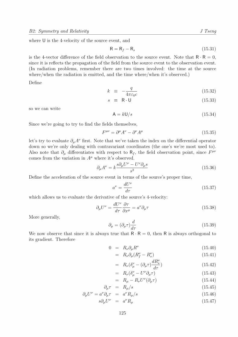
B2: Symmetry and Relativity J Tseng
where U is the 4-velocity of the source event, and
R = Rf − Rs (15.31)
is the 4-vector difference of the field observation to the source event. Note that R · R = 0,since it is reflects the propagation of the field from the source event to the observation event.(In radiation problems, remember there are two times involved: the time at the sourcewhere/when the radiation is emitted, and the time where/when it’s observed.)
Define
k ≡ − q
4πε0c(15.32)
s ≡ R · U (15.33)
so we can writeA = kU/s (15.34)
Since we’re going to try to find the fields themselves,
F µν = ∂µAν − ∂νAµ (15.35)
let’s try to evaluate ∂µAν first. Note that we’ve taken the index on the differential operator
down so we’re only dealing with contravariant coordinates (the one’s we’re most used to).Also note that ∂µ differentiates with respect to Rf , the field observation point, since F µν
comes from the variation in Aµ where it’s observed.
∂µAν = k
s∂µUν − Uν∂µs
s2(15.36)
Define the acceleration of the source event in terms of the source’s proper time,
aν =dU ν
dτ(15.37)
which allows us to evaluate the derivative of the source’s 4-velocity:
∂µUν =
dU ν
dτ
∂τ
∂xµ= aν∂µτ (15.38)
More generally,
∂µ = (∂µτ)d
dτ(15.39)
We now observe that since it is always true that R · R = 0, then R is always orthogonal toits gradient. Therefore
0 = Rν∂µRν (15.40)
= Rν∂µ(Rνf −Rν
s) (15.41)
= Rν(δνµ − (∂µτ)
dRνs
dτ) (15.42)
= Rν(δνµ − Uν∂µτ) (15.43)
= Rµ −RνUν(∂µτ) (15.44)
∂µτ = Rµ/s (15.45)
∂µUν = aν∂µτ = aνRµ/s (15.46)
s∂µUν = aνRµ (15.47)
125

B2: Symmetry and Relativity J Tseng
For the second term, we need
∂µs = ∂µ(RνUν) (15.48)
= (∂µRν)Uν +Rν(∂µU
ν) (15.49)
= (δνµ − Uν∂µτ)Uν +Rν(aν∂µτ) (15.50)
= Uµ − UνUνRµ
s+Rνa
νRµ
s(15.51)
= Uµ +Rµ
s(c2 + R · a) (15.52)
Uν∂µs = UνUµ +Rµ
s(c2 + R · a)Uν (15.53)
Combining,
∂µAν =
k
s2(aνRµ − UνUµ −
Rµ
s(c2 + R · a)Uν) (15.54)
= − ks2UνUµ −
kc2Rµ
s3(− s
c2aν + Uν +
1
c2(R · a)Uν) (15.55)
= − ks2UνUµ −
kc2
s3RµU
ν (15.56)
∂µAν = − ks2UνUµ − kc2
s3RµUν (15.57)
where
Uν ≡ Uν − 1
c2(saν − Uν(R · a)) (15.58)
Combining into F µν , the first term drops out, so
F µν = ∂µAν − ∂νAµ (15.59)
= −kc2
s3(RµUν −RνUµ) (15.60)
=qc
4πε0
RµUν −RνUµ
(R · U)3(15.61)
To evaluate the field itself, we choose a frame in which the source moves (i.e., a frame of adevice in which the charges move):
R = (r, r) (15.62)
U = γ(c,u) (15.63)
s = gµνRµUν = γ(−cr + r · u) = −cγ(r − r · u
c) (15.64)
(Remember that we’re using the metric −+ ++)
We will also need the acceleration. Because we’re evaluating in the device’s frame, the propertime is the same as the time at the source.
aµ =dUµ
dτ=
(dγ
dτc,dγ
dτu + γ
du
dτ
)= γ(γc, γu + γa) (15.65)
126

B2: Symmetry and Relativity J Tseng
The expression for the electric field is
Ei = cF 0i =−kc3
s3(R0U i −RiU0) (15.66)
So we evaluate the modified velocities:
R · a = gµνRµaν = γ(−γrc+ γu · r + γa · r) (15.67)
U0 = U0 − 1
c2(sa0 − U0(R · a)) (15.68)
= γc− 1
c2(γ(r · u)γγc− γcrγγc− γ2c(γa · r + γu · r− γrc)) (15.69)
= γc+ γ3 a · rc
(15.70)
U i = U i − 1
c2(sai − U i(R · a)) (15.71)
= γu− 1
c2(γ(u · u− cr)(γγu− γ2a)− γu(γ2a · r + γγu · r− γγrc)) (15.72)
= γu− 1
c2(γu(γγr · u− γγcr − γ2a · r− γγu · r + γγrc) + γ3a(r · u− cr))(15.73)
= γu +γ3
c2(a · r)u− γ3
c2(r · u− cr)a (15.74)
= γu +γ3
c2(a · r)u +
γ2
c2sa (15.75)
Then after a fair amount of tedious algebra (as if this wasn’t already), and taking advantageof the vector algebra rule
a ∧ (b ∧ c) = (a · c)b− (a · b)c (15.76)
we get the formula
E =q
4πε0(r − r · u/c)3
[r− ur/c
γ2− r ∧ ((r− ur/c) ∧ a)
c2
](15.77)
In summary (Steane),
E =q
4πε0κ2
(n− v/c
γ2r2+
n ∧ [(n− v/c) ∧ a]
c2r
)(15.78)
B = n ∧ E/c (15.79)
n = r/r (15.80)
κ = 1− vrc
= 1− n · vc
(15.81)
15.3 *Half-wave electric dipole antenna
For an antenna, we haveωd0 = ωqL = IL (15.82)
127

B2: Symmetry and Relativity J Tseng
where I is the ac current in a short wire of length L. Then
E = cB =ω2d0
4πε0c2sin(ωt− kr)sin θ
r(15.83)
= − iI
2ε0c
L
λ
sin θ
rei(kr−ωt) (15.84)
where one takes the real part to get the field value. Note that the current goes as d ∼ cosωt,so is 1/4 out of phase.
A half-wave dipole antenna is designed with L = λ/2, so the maximum current oscillationis at the center, and zero at the ends; one feeds in power at the center. This maximizes thepower output for the antenna. The current as a function of position in the antenna is
I = I0 cos kz (15.85)
so that, integrating, ∫Idz = I0
λ
π(15.86)
which leads to fields (replacing IL with the integral)
E = cB ≈ − iI0
2πε0c
sin θ
rei(kr−ωt) (15.87)
15.3.1 *Radiated power
To calculate the power, we work from the radiation field, ignoring the near Coulomb field
Erad =q
4πε0κ3
n ∧ [(n− v/c) ∧ a]
c2r(15.88)
Brad =n ∧ Erad
c(15.89)
n ≡ r/r (15.90)
κ ≡ 1− vr/c = 1− n · v/c (15.91)
For v/c 1,
Erad ≈q
4πε0c2
(n ∧ (n ∧ a)
r
)(15.92)
We also ignore diffraction effects, and the energy required to power the antenna itself.
The Poynting vector is
N ≡ ε0c2E ∧B (15.93)
= ε0cErad ∧ (n ∧ Erad) (15.94)
= ε0c[(Erad · Erad)n− (Erad · n)Erad] (15.95)
128

B2: Symmetry and Relativity J Tseng
We see that the second term is zero because we can define b = n ∧ a and
Erad · n ∝ (n ∧ b) · n (15.96)
= (n ∧ n) · b (15.97)
= 0 (15.98)
ThereforeN = ε0cE
2radn (15.99)
An easy way to evaluate E2rad is
E2rad ∝ (n ∧ b) · (n ∧ b) (15.100)
= n · [b ∧ (n ∧ b)] (15.101)
= n · [b2n− (b · n)b] (15.102)
= b2 − (n · b)2 (15.103)
We know that n · b = n · (n ∧ a) = 0 and b2 = a2 sin2 θ, where θ is the angle between a(parallel to the orientation of the dipole) and the radial direction n.
E2rad =
(q
4πε0c2
)2a2 sin2 θ
r2(15.104)
N = ε0c
(q
4πε0c2
)2a2 sin2 θ
r2n (15.105)
(15.106)
We see that the energy flux is purely radial. The differential power is
dP
dΩ= Nr2 =
q2
4πε0c3
1
4πa2 sin2 θ (15.107)
This is the power flux into an area r2dΩ. The sin2 θ distribution is characteristic of a dipole.
The total power is then
PL =
∫dΩ
dP
dΩ(15.108)
=q2
4πε0c3
1
4πa22π
∫ 1
−1
(1− cos2 θ)d cos θ (15.109)
=q2
4πε0c3
a2
2(2− 2
3) (15.110)
=2
3
q2
4πε0
a2
c3(15.111)
which as we see does not diminish with r. This is the Larmor formula for a non-relativisticaccelerating charge.
For the relativistic case, we note that P must be an invariant, and we’re looking for a formulawhich reduces to PL when β → 0. Previous expressions for E and B indicate that the only
129
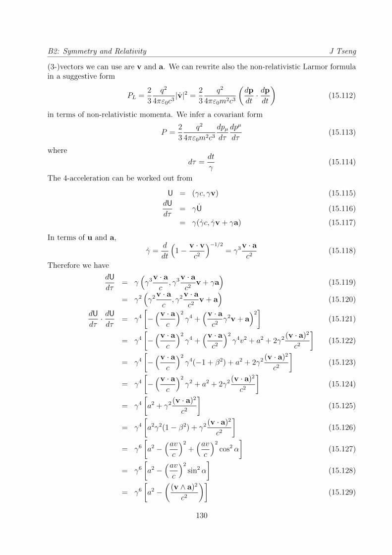
B2: Symmetry and Relativity J Tseng
(3-)vectors we can use are v and a. We can rewrite also the non-relativistic Larmor formulain a suggestive form
PL =2
3
q2
4πε0c3|v|2 =
2
3
q2
4πε0m2c3
(dp
dt· dpdt
)(15.112)
in terms of non-relativistic momenta. We infer a covariant form
P =2
3
q2
4πε0m2c3
dpµdτ
dpµ
dτ(15.113)
where
dτ =dt
γ(15.114)
The 4-acceleration can be worked out from
U = (γc, γv) (15.115)
dU
dτ= γU (15.116)
= γ(γc, γv + γa) (15.117)
In terms of u and a,
γ =d
dt
(1− v · v
c2
)−1/2
= γ3 v · ac2
(15.118)
Therefore we have
dU
dτ= γ
(γ3 v · a
c, γ3 v · a
c2v + γa
)(15.119)
= γ2(γ2 v · a
c, γ2 v · a
c2v + a
)(15.120)
dU
dτ· dUdτ
= γ4
[−(v · a
c
)2
γ4 +(v · ac2
γ2v + a)2]
(15.121)
= γ4
[−(v · a
c
)2
γ4 +(v · ac2
)2
γ4v2 + a2 + 2γ2 (v · a)2
c2
](15.122)
= γ4
[−(v · a
c
)2
γ4(−1 + β2) + a2 + 2γ2 (v · a)2
c2
](15.123)
= γ4
[−(v · a
c
)2
γ2 + a2 + 2γ2 (v · a)2
c2
](15.124)
= γ4
[a2 + γ2 (v · a)2
c2
](15.125)
= γ4
[a2γ2(1− β2) + γ2 (v · a)2
c2
](15.126)
= γ6
[a2 −
(avc
)2
+(avc
)2
cos2 α
](15.127)
= γ6
[a2 −
(avc
)2
sin2 α
](15.128)
= γ6
[a2 −
((v ∧ a)2
c2
)](15.129)
130

B2: Symmetry and Relativity J Tseng
Combining, we obtain the Lienard result
P =2
3
q2
4πε0c3γ6
[a2 − (v ∧ a)2
c2
](15.130)
15.3.2 Energy loss in accelerators
Particle accelerators generally come in two varieties, linear and circular. Linear acceleratorsadd energy to a beam only once as it passes along the machine, so important limitationscome from how long they can be built, and how strong their accelerating elements can bemade.
Circular accelerators have the advantage of being able to add energy to a beam many timesas it recirculates in the machine. The drawback is one then has to bring the beam back (thusthe circle). This means that for most of the distance around the accelerator, one redirectsthe beam without actually adding any energy to it.
The acceleration is
a =v2
ρ=β2c2
ρ(15.131)
where ρ is the orbit radius. The radiated power (loss) from Larmor’s formula is
PL =2
3
q2
4πε0c3γ6 1
γ2
β4c4
ρ2=
2
3
q2c
4πε0ρ2β4γ4 (15.132)
The energy loss per revolution is
∆E =P
f=
2πρ
βcP =
4π
3
q2
4πε0ρβ3γ4 =
4π
3
α~cρβ3
(E
mc2
)4
(15.133)
where α = 1/137 is the fine structure constant, ~c = 197 MeV fm, E is the beam energy,and m is the mass of the beam particle.
In some of the first electron synchrotrons,
ρ ∼ 1 m (15.134)
Emax ∼ 0.3 GeV (15.135)
which ends up around 1 keV per revolution. This is less than the energy gain of a few keVper turn, but not negligible. On the other hand, for LEP this amounted to O(0.1%) energyloss per revolution and was measured in megawatts, so a lot of energy was expended justkeeping the beam at the same energy. (And one more “on the other hand”: this powerloss, in the form of “synchrotron radiation”, is actually useful in other branches of physics,chemistry, and biology because it is a source of high-intensity light—and thus, for example,specially built facilities such as the Diamond Light Source. One field’s annoyance is anotherfield’s opportunity.)
For the LHC, this effect is much suppressed because protons are 2000 times more massivethan electrons. The LHC is the first proton accelerator where the synchrotron radiation iseven noticeable.
131

Chapter 16
Energy-momentum tensor
Earlier, we obtained for the energy density and flux
u =1
2µ0
(B2 +
E2
c2
)(16.1)
N =1
µ0
E ∧B (16.2)
We also had a continuity equation
∂u
∂t+∇ ·N = −j · E (16.3)
One might be tempted to put u and N into a 4-vector N and write the equation in the form
∂µNν =? (16.4)
but j ·E isn’t a proper 4-vector. If anything, it appears to be a time-like component of F0µJµ.
This suggests that u and N are really part of another object. This is the “stress-energy”tensor, which describes momentum flows within a body. It was originally used to describemechanical stresses and how forces change directions, but it applies to any system which canbe described with a field. In the case of the electromagnetic field, it is often divorced fromits mechanical origin and called the “energy-momentum” tensor.
The elements of an arbitrary stress-energy tensor can be interpreted as follows
T 00 energy densityT 0j energy fluxT j0 momentum densityT jj pressureT ij, i 6= j shear stress
The space elements of the tensor represent the momentum flux. There’s not a guaranteethat this tensor is symmetric, but it’s also ambiguous up to a 4-divergence, i.e., one can adda 4-divergence term which will not affect any physics.
132

B2: Symmetry and Relativity J Tseng
The units of the tensor elements are of force per unit area, or pressure.
We would like to assign the energy density to T 00. And since the Poynting vector representsenergy flow, it should find its place in T 0i. But to get a better picture of the tensor, let’slook at some fluid examples first.
(The symmetric rank-2 tensor field is a member of the (1, 1) representation space. It showsup as a spin-2 graviton.)
16.1 Fluid examples
The simplest fluid we can envisage is something like a dust cloud: in its rest frame, there isno stress, and the only energy comes from the rest masses of the particles themselves. So inthe cloud’s rest frame, we have
T µν =
ρ0c
2
00
0
(16.5)
where ρ0 is the mass density.
Now let’s give the cloud an overall motion 4-vector U. If we choose a direction x, then theamount of dust crossing a plane of constant x is clearly proportional to ux. The amount ofmomentum crossing with each dust particle is also proportional to ux. Similarly, the amountof y momentum crossing with each dust particle is proportional to uy.
This leads us to a simple form of the stress-energy tensor:
T µν = ρ0UµUν (16.6)
which we also might have expected from the fact that we only had ρ0 and U out of which tofashion the tensor.
For an ideal fluid, there is no heat conduction, and no viscosity. These conditions imply thatT 0i = T i0 = 0 and T ij = 0 for i 6= j. In its rest frame, there should be an energy densityρ0c
2 and pressure p.
T µν =
ρ0c
2
pp
p
(16.7)
If we build the tensor out of 4-velocities as before, we expect it to have the form
T µν = (ρ0 +p
c2)UµUν + pgµν (16.8)
(If we use a metric with a different signature, the sign of the second term can change.)
133

B2: Symmetry and Relativity J Tseng
16.2 *Energy-momentum tensor of the EM field
Returning to the electromagnetic field, how can we fit the energy density and Poynting vectorinto the tensor and still have T µν constructed out of other tensors? Let’s start with T 0i.Since it is a cross product between E and B, it suggests a contraction within F µν
1
c(E ∧B)i = gµνF
0µF νi (16.9)
We assign this to T 0i. But if we extend this to the time-time component, we get
gµνF0µF ν0 = −E2/c2 (16.10)
so we “fix this up” by adding an invariant term for diagonal terms.
FµνFµν = 2
(B2 − E2
c2
)(16.11)
In the end, we work with the following:
T µν =1
µ0
[−1
4(FαβF
αβ)gµν − F µγF
γν
](16.12)
With any luck, we’ll be able to look at some more methodical derivations in the last fewlectures.
When we look at the components, we find
T µν =
1
2µ0(B2 + E2
c2) Nx/c Ny/c Nz/c
Nx/c P11 P12 P13
Ny/c P21 P22 P23
Nz/c P31 P32 P33
(16.13)
The spatial elements
Pij ≡1
µ0
[1
2δij(B
2 +E2
c2)− (BiBj +
EiEjc2
)
](16.14)
then form the momentum flux tensor.
Now the form-invariant generalization of Poynting’s theorem is
∂αTαβ = 0 (16.15)
It is also worth looking at the angular momentum of the electromagnetic field,
Lfield =
∫x ∧ (E ∧B)d3x (16.16)
The generalization is a rank-3 tensor
Mαβγ = Tαβxγ − Tαγxβ (16.17)
134

B2: Symmetry and Relativity J Tseng
Angular momentum conservation is
∂αMαβγ = ∂αT
αβxγ − ∂αTαγxβ (16.18)
= (∂αTαβ)xγ + T γβ − (∂αT
αγ)xβ − T βγ (16.19)
= T γβ − T βγ (16.20)
= 0 (16.21)
which is zero because of the symmetry of the stress-energy tensor.
16.3 *Applications with simple geometries
16.3.1 *Parallel-plate capacitor
A parallel-plate capacitor with area A oriented with its gap along the x direction has aconstant electric field Ex. The charge on each plate is
Q = Aε0E (16.22)
so the force pulling the plates together is
f =QE
2= ε0A
E2
2(16.23)
The stress tensor is
T µν =ε0E
2
2
1−1
11
(16.24)
The energy density and pressure are as expected, the pressure being negative since the platesare being pulled together. There is also an outward pressure which reflects the tension amongthe field lines.
16.3.2 *Long straight solenoid
This case is similar to the parallel-plate capacitor, with a similar layout of field lines. Thestress tensor is
T µν =ε0c
2B2
2
1−1
11
(16.25)
135

B2: Symmetry and Relativity J Tseng
16.3.3 *Plane waves
Let’s examine a plane wave travelling in the x direction, polarized along the y direction:
E = (0, E, 0) cos(ωt− kx) (16.26)
B = (0, 0, B) cos(ωt− kx) (16.27)
B =E
c=kE
ω(16.28)
The energy density is
B2 +E2
c2=
2E2
c2(16.29)
The Poynting vector is
N =1
µ0
E ∧B =1
µ0
xEB cos2(ωt− kx) (16.30)
= xE2
µ0ccos2(ωt− kx) (16.31)
The plane wave therefore carries energy in the x direction (as expected), and we should seethat it exerts a pressure (momentum flow) in the x direction as well:
P11 =1
2µ0
2E2
c2− 1
µ0
(B2x +
E2x
c2) =
E2
µ0c2(16.32)
P22 =1
2µ0
2E2
c2− 1
µ0
(B2y +
E2y
c2) = 0 (16.33)
P33 =1
2µ0
2E2
c2− 1
µ0
(B2z +
E2z
c2) = 0 (16.34)
The stress tensor is therefore
T µν =E2
µ0c2cos2(ωt− kx)
1 11 1
00
(16.35)
A more general way to write this tensor admits any direction:
T µν =E2 cos2(K · X)
µ0c2ω2KµKν (16.36)
whereK = (ω/c, k, 0, 0) (16.37)
is the 4-wavenumber vector. An interesting side-note on this way of writing the tensor isthat the quotient rule, which states that an object which contracts with a tensor to produceanother tensor must itself be a tensor, implies (E/ω)2 is a (rank-0) tensor, i.e., a scalar.
136

Chapter 17
Noether’s theorem
In this chapter, we’ll develop the connection between a symmetry and a conservation law asshown in Noether’s Theorem.
Emmy Noether actually proved two theorems in her 1918 paper. The first, which links globalsymmetries with conservation laws, is the most widely used and taught. As a result (and asusual for important physics), it has gone through a number of mutations and simplificationsas it has been taught and re-taught. What is presented here is thus not the original form ofNoether’s Theorem, but a simpler “modern” form.
The second theorem has recently gotten some more attention: it shows dependencies betweenequations of motion imposed by “local” symmetries. See KA Barding (Studies in Historyand Philosophy of Modern Physics, 33 (2002) 3-22). It is beyond the scope of this course todiscuss these local symmetries in detail, but we’ll take a peek at one of the most important,that of “local gauge invariance”, a principle embedded deeply into how we understand thephysics of elementary particles. Which is, when you think of it, pretty remarkable for atheorem which was proven in the context of classical, non-quantum physics.
17.1 Discrete systems
(based on Banados and Reyes, arxiv 1601.03616v2)
Noether’s (First) Theorem applies to any system that can be derived from an action andpossesses some continuous (non-gauge) symmetry.
There are two kinds of symmetry at play. First, there’s a loose form of invariance in theform of the action. Second, there’s an invariance in the action with respect to variationsaround the classical path. Noether’s Theorem involves equating the two.
137

B2: Symmetry and Relativity J Tseng
17.1.1 Action invariance
The action is a functional of a path, I[qk(t)], for k generalized coordinates which are afunction of the variable t (which looks like time, but is in reality a dummy variable).
I[qk(t)] =
∫L(qk(t), qk(t))dt (17.1)
The path is now modified by a (small) function fk(t). The change in the action is
δI[qk(t), fk(t)] = I[qk(t) + fk(t)]− I[qk(t)] (17.2)
In its strictest form, fk(t) is a symmetry if δI = 0 for all paths qk(t). We can be a bit looser,however, and let the difference include a “boundary term”:
δI[qk(t), fk(t)] = I[qk(t) + fk(t)]− I[qk(t)] =
∫dtdK
dt(17.3)
This is the same as modifying the L by adding a term dK/dt. It should be emphasized thatfk(t) is a symmetry if this is true for arbitrary paths qk(t).
In the literature (and subsequently in these lectures), fk(t) is usually written as δqk(t),which does remind us that it’s supposed to be small. On the other hand, it tends to makeus think it’s somehow related to the qk(t). It’s not. The functions fk(t) implement thetransformation over which the action is invariant, whereas qk(t) represent any path (amongwhich is the classical path which solves the Euler-Lagrange equations).
17.1.2 On-shell variation
In this case, we start from the classical path qk(t) = qk(t) which already solves the Euler-Lagrange equations.
0 =d
dt
(∂L
∂qk
)− ∂L
∂qk(17.4)
Then we take the variation δqk(t) to be arbitrary but small. (In this sense it’s the oppositeof the previous type of variation.)
The change in action is then
δI[qk, δqk] = I[qk + δqk]− I[qk] (17.5)
=
∫dt
(L(qk, qk) +
∂L
∂qkδqk +
∂L
∂qkδqk − L(qk, qk)
)(17.6)
138

B2: Symmetry and Relativity J Tseng
We use integration by parts∫dtd
dt(a(t)b(t)) =
∫dtda
dtb+
∫dta
db
dt(17.7)∫
dtd
dt
(∂L
∂qkδqk)
=
∫dt∂L
∂qkd
dt(δqk) +
∫dtd
dt
(∂L
∂qk
)δqk (17.8)
=
∫dt∂L
∂qkδqk +
∫dtd
dt
(∂L
∂qk
)δqk (17.9)∫
dt∂L
∂qkδqk =
∫dtd
dt
(∂L
∂qkδqk)−∫dtd
dt
(∂L
∂qk
)δqk (17.10)
to remove the time derivative in δqk
δI[qk, δqk] =
∫dt
[∂L
∂qk− d
dt
(∂L
∂qk
)]δqk +
∫dtd
dt
(∂L
∂qkδqk)
(17.11)
=
∫dtd
dt
(∂L
∂qkδqk)
(17.12)
where we’ve used the fact that qk(t) solves the Euler-Lagrange equations.
17.1.3 Noether’s Theorem
If we denote fk(t) as δsqk(t) to indicate the action symmetry, and qk(t) to denote the classical
path,
δI[qk(t), δsqk(t)] =
∫dtdK
dt(17.13)
δI[qk(t), δqk(t)] =
∫dtd
dt
(∂L
∂qkδqk)
(17.14)
We now relate the form invariance to the on-shell variation by setting qk(t) = qk(t) andδqk(t) = δsq
k(t) in the two formulae and equating the δI’s.
δI[qk(t), δsqk(t)] =
∫dt
(dK
dt
)=
∫dtd
dt
(∂L
∂qkδsq
k
)(17.15)
Setting the two δI’s equal leads to this simplified version of Noether’s First Theorem, thatgiven a symmetry δsq
k(t), there is a quantity
Q = K − ∂L
∂qkδsq
k (17.16)
which is conserved.
In practice, the Q calculated here will not be the conserved current as usually conceived; itwill be a conserved current multipled by infinitesimal parameters of the symmetry. Sincethese are arbitrary parameters, we drop them and extract the conserved current itself. Some
139

B2: Symmetry and Relativity J Tseng
treatments of the theorem (including Noether’s own) carry these parameters (which we callεj for illustration) through by writing
K =∑j
∂K
∂εjεj (17.17)
δqk =∑j
∂(δqk)
∂εjεj (17.18)
up to the point where the two δI’s are equated: at this point, the “arbitrary parameters”argument is invoked to equate each εj term separately and thus cancel the εj’s. Nowadays,it is more common to drop the parameters at the very last stage.
17.1.4 Examples
We’ll use examples from non-relativistic problems with an distance-dependent interactionpotential. The Lagrangian is
L =∑i
1
2miri
2 − 1
2
∑j 6=i
V (|ri − rj|) (17.19)
and its action
I[ri(t)] =
∫dt
(∑i
1
2miri
2 − 1
2
∑j 6=i
V (|ri − rj|)
)(17.20)
The second sum is taken over all pairs of i and j where j 6= i. Since the potential is symmetricwith respect to each pair of bodies, the sum includes two identical terms for each pair, andthus the 1/2 factor in front.
Rotations
First, we note that the Lagrangian and action are invariant with respect to simultaneousrotations of all the ri,
ri(t)→ r′i(t) = Rri(t) (17.21)
where R is an orthogonal matrix. Clearly the potential is invariant with respect to such arotation of all the bodies:
V (|r′i − r′j|) = V (|Rri −Rrj|) (17.22)
= V (|R(ri − rj)|) (17.23)
= V (|ri − rj|) (17.24)
For the kinetic energy part, we need to rephrase the rotation as an infinitesimal change (sincewe’re concerned with continuous symmetries). For small rotations,
Rri = ri +α ∧ ri +O(α2) (17.25)
140

B2: Symmetry and Relativity J Tseng
where α is a small, constant vector. The small change is then
fi(t) = α ∧ ri(t) (17.26)
so that
r′i(t) = ri +α ∧ ri (17.27)
r′2i = r2i + 2ri · (α ∧ ri) +O(α2) (17.28)
= r2i + 2α · (ri ∧ ri) +O(α2) (17.29)
= r2i +O(α2) (17.30)
We see from this that the kinetic energy also remains unchanged to first order. The actionis invariant, with the boundary term K = 0.
Since the boundary term vanishes, the conserved current comes from the on-shell variation,
Q = −∑i,k
∂L
∂rkiδsr
ki (17.31)
= −∑i
miri · (α ∧ ri) (17.32)
=∑i
miα · (ri ∧ ri) (17.33)
= α ·
(∑i
mi(ri ∧ ri)
)(17.34)
Since α is really three arbitrary constants, we find we have three conserved currents
dL
dt=
d
dt
(∑i
miri ∧ ri
)= 0 (17.35)
which is of course total angular momentum conservation for a distance-dependent interactionpotential.
Translations
Using the same action as before, let
ri(t)→ r′i(t) = r(t)− εri(t) (17.36)
fi(t) = −εri(t) (17.37)
with ε a constant.
I[r′i] =
∫dt
(∑i
1
2mi(ri − εri)2 − 1
2
∑j 6=i
V (|ri − εri − rj + εrj|)
)(17.38)
141

B2: Symmetry and Relativity J Tseng
The first sum, to first order, is∫dt∑i
(1
2mir
2i − εmiri · ri) =
∫dt∑i
(1
2mir
2i −
1
2εmi
dridt
) (17.39)
For the second (potential) term, it is useful to think of the potential as a function of r2ij =
(ri − rj)2. For each pair i and j, we have to first order
V ((ri − rj − εri + εrj)2) = V ((rij − εrij)2) (17.40)
= V (r2ij − 2εrij · rij +O(ε2)) (17.41)
= V (r2ij)− 2εrij · rij
(dV
d(r2ij)
)(17.42)
= V (r2ij)−
d(r2ij)
dt
(dV
d(r2ij)
)(17.43)
= V (r2ij)−
dV
dt(17.44)
Combining and taking the difference,
δI[r, f ] = −ε∫dx
d
dt
(∑i
1
2mir
2i −
1
2
∑j 6=i
V (r2ij)
)(17.45)
so this is a symmetry with boundary term
K = −ε
(∑i
1
2mir
2i −
1
2
∑j 6=i
V (r2ij)
)= −εL (17.46)
The physical interpretation of this symmetry can be seen by considering a path which isdisplaced wholesale in time:
q′(t+ ε) = q(t) (17.47)
In order to evaluate δI consistently, we need to find q′ as a function of t, not t+ ε.
q′(t) = q(t− ε) = q(t)− εq(t) +O(ε2) (17.48)
so we see that the f(t) given above is the infinitesimal version of a time translation.
For the on-shell variation, we have for each body i (and implicitly summing over the com-ponents k)
∂L
∂rkiδsr
ki = mir
ki (−εrki ) = −εmir
2i (17.49)
from which follows the conserved current
Q = −ε
(∑i
1
2mir
2i −
1
2
∑j 6=i
V (r2ij)−
∑i
mir2i
)(17.50)
= ε
(∑i
1
2mir
2i +
1
2
∑j 6=i
V (r2ij)
)= εE (17.51)
from which we see that time invariance leads to the conservation of total energy in the centralforce problem.
142

B2: Symmetry and Relativity J Tseng
Translations in Special Relativity
We can write down a relativistic Lagrangian with an interacting potential of the form
L = −∑i
mic(−UµUµ)1/2 −∑j 6=i
V ((xi − xj)µ(xi − xj)µ) (17.52)
The first term is one of the usual “kinetic” terms. The second potential is a function of theinvariant interval between two bodies. For instance, the potential could be a delta functionwhich selects only those pairs which could be causally connected via a null vector. All of ourearlier collision problems would fall in this category.
The translation takes the formx′µi = xµi − εµ (17.53)
where the εµ are four constant displacements. From this, it is easy to see that
U ′i = Ui (17.54)
(x′i − x′j) = (xi − xj) (17.55)
and therefore the Lagrangian is form-invariant, so K = 0.
To evaluate the on-shell variation,
∂(−UµUµ)
∂Uα=
∂
∂Uα(−gµνUµUν) (17.56)
= −gµν(δµαUν + Uµδνα) (17.57)
= −gανUν − gµαUµ (17.58)
= −2gαµUµ (17.59)
so we get for each Ui
∂L
∂(Uα)= −mic(−UµUµ)−1/2 1
2(−2gανU
ν) (17.60)
= migανUν (17.61)
= Pα (17.62)
The conserved current is then
Q = K −∑i
∂L
∂(Uαi )δs(xi)α (17.63)
but since δs(xi)α is simply εα, and (as in the case of the rotation example above) these arearbitrary constants, what we end up with are four conserved currents
Qα =∑i
(Pi)α (17.64)
Thus we see that from translational symmetry we get the 4-momentum conservation wementioned at the very beginning of the course.
143

B2: Symmetry and Relativity J Tseng
17.2 Noether’s Theorem for classical fields
The change from discrete particles to fields is not difficult.
Some discussions of Noether’s Theorem also discuss change of coordinates, but it’s easiestto restrict ourselves to changes in fields. We’ve seen that a change in coordinates canbe implemented as a change in fields, so we’ll restrict ourselves to the latter category ofvariations. This also helps us distinguish from trivial changes which aren’t connected tosymmetries at all, such as changing or substituting for dummy variables in integrals.
A set of symmetries is a set of infinitesimal functions δsφ(x) such that
δI[φ, δsφ] = I[φ(x) + δsφ(x)]− I[φ(x)] =
∫d4x∂µK
µ (17.65)
for all φ(x). The last term corresponds to the “boundary term”. Note that the δsφ(x) don’tinvolve any changes to coordinates (which in fields function as labels).
The on-shell variation starts from the action
I[φ(x)] =
∫d4xL(φ, ∂µφ) (17.66)
and the solution to the Euler-Lagrange equation:
0 = ∂µ
(∂L
∂(∂µφ)
)− ∂L∂φ
(17.67)
We call the solution φ(x), and then consider the arbitrary but small variation δφ(x).
δI[φ, δφ] =
∫d4x
(∂L∂φ
δφ+∂L
∂(∂µφ)δ(∂µφ)
)(17.68)
=
∫d4x
(∂L∂φ
δφ− ∂µ(
∂L∂(∂µφ)
)δφ
)+
∫d4x∂µ
(∂L
∂(∂µφ)δφ
)(17.69)
=
∫d4x∂µ
(∂L
∂(∂µφ)δφ
)(17.70)
where the last step takes advantage of the fact that φ solves the Euler-Lagrange equation.
Equating the δI’s as before, we get
0 =
∫d4x∂µ
(∂L
∂(∂µφ)δsφ−Kµ
)=
∫d4x∂µJ
µ (17.71)
where
Jµ =∂L
∂(∂µφ)δφ(x)−Kµ (17.72)
is the conserved current. The derivative ∂µ is, as before, a “total partial derivative”. Inpractice, since Jµ is usually written as a function of the coordinates only, this equation isoften seen in the form
0 = ∂µJµ (17.73)
144

B2: Symmetry and Relativity J Tseng
In the case that J drops to zero at large distances (one needs to check this, as it isn’t alwaystrue), we can write
0 = ∂µJµ =
∂J0
∂t+∇ · J (17.74)
If we take the spatial volume integral, we have for the first term∫V
d3x∂J0
∂t=
d
dt
∫V
d3xJ0 =dQ
dt(17.75)
In the first equality, the “total partial derivative” has become a full derivative, because we’veintegrated out the other coordinates. For the second term∫
V
d3x∇ · J =
∫S
J · da = 0 (17.76)
so we getdQ
dt= 0 (17.77)
with Q the conserved quantity.
17.2.1 Translations
Let’s look at a scalar field with the Klein-Gordon Lagrangian:
L = −1
2(∂µφ)(∂µφ)− 1
2m2φ2 (17.78)
Consider the translationxµ → xµ + εµ (17.79)
which becomes the field transformation
φ(xµ)→ φ(xµ − εµ) ≈ φ(xµ)− εµ∂µφ(xµ) (17.80)
The change in the Lagrangian density is then
δL = −1
2(∂µ(φ− εν∂νφ))(∂µ(φ− ελ∂λφ))− 1
2m2(φ− εν∂νφ)2 (17.81)
+1
2(∂µφ)(∂µφ) +
1
2m2φ2 (17.82)
= −1
2(∂µφ− εν∂ν∂µφ)(∂µφ− ελ∂λ∂µφ)− 1
2m2(φ− εν∂νφ)2 (17.83)
+1
2(∂µφ)(∂µφ) +
1
2m2φ2 (17.84)
= εν(∂ν∂µφ)(∂µφ) +m2ενφ∂νφ (17.85)
= εν [(∂ν∂µφ)(∂µφ) +m2φ∂νφ] (17.86)
= ∂ν [1
2εν(∂µφ)(∂µφ) +
1
2m2ενφ2] (17.87)
= ∂ν [−ενL] (17.88)
145

B2: Symmetry and Relativity J Tseng
Which gives a boundary termKλ = −ελL (17.89)
and therefore a conserved current
Jλ =∂L
∂(∂λφ)δφ−Kλ = (−∂λφ)(−εµ∂µφ) + ελL = εµT λµ (17.90)
where
T λµ = (∂λφ)(∂µφ) + δλµL (17.91)
T λµ = (∂λφ)(∂µφ) + gλµL (17.92)
which is the “canonical” energy-momentum (stress-energy) tensor. The conservation lawtakes the form
0 = ∂µTµν (17.93)
which is actually four conservation laws (conserved currents) at once.
17.2.2 Complex fields
We saw earlier that the Klein-Gorden equation can be used to describe two independentfields with identical mass. We can look at them from the perspective of Noether’s Theoremto see more of their relationship.
L = −1
2(∂µφ
∗)(∂µφ)− 1
2m2φ∗φ (17.94)
A unitary transformation of the fields gives for the two fields
φ′ = eiλφ (17.95)
φ∗′ = e−iλφ∗ (17.96)
(I happen to be giving priority to the asterisk rather than the ’, since we’re really considerφ∗ as an independent field which we happening to be transforming.)
If we turn these into infinitesimal changes,
δφ = iλφ (17.97)
δφ∗ = −iλφ∗ (17.98)
Pauli called this a “gauge transformation of the first kind”.
The form variation in the Lagrangian density is
δL[φ, φ∗, φ′, φ∗′] = L[φ+ δφ, φ∗ + δφ∗]− L[φ, φ∗] (17.99)
= L[φ+ iλφ, φ∗ − iλφ∗]− L[φ, φ∗] (17.100)
= −1
2(∂µ(φ∗ − iλφ∗))(∂µ(φ+ iλφ)) (17.101)
−1
2m2(φ∗ − iλφ∗)(φ+ iλφ) (17.102)
= L · (1 + λ2) (17.103)
= L+O(λ2) (17.104)
146

B2: Symmetry and Relativity J Tseng
The on-shell variation in the Lagrangian density is
δL =∂L∂φ
δφ+∂L
∂(∂µφ)δ(∂µφ) +
∂L∂φ∗
δφ∗ +∂L
∂(∂µφ∗)δ(∂µφ
∗) (17.105)
We note that
δ
(∂φ
∂xµ
)=∂(δφ)
∂xµ(17.106)
and thus the second term is
∂L∂(∂µφ)
∂(δφ)
∂xµ= ∂µ
(∂L
∂(∂µφ)δφ
)− ∂µ
(∂L
∂(∂µφ)
)δφ (17.107)
and similarly for the fourth term. Assuming then that φ and φ∗ already satisfy the Euler-Lagrange equations,
δL = ∂µ
(∂L
∂(∂µφ)δφ
)+
[∂L∂φ− ∂µ
(∂L
∂(∂µφ)
)]δφ (17.108)
+∂µ
(∂L
∂(∂µφ∗)δφ∗)
+
[∂L∂φ∗− ∂µ
(∂L
∂(∂µφ∗)
)]δφ∗ (17.109)
= ∂µ
(∂L
∂(∂µφ)δφ+
∂L∂(∂µφ∗)
δφ∗)
(17.110)
= − i2λ∂µ[(∂µφ∗)φ− φ∗(∂µφ)] (17.111)
Setting δL = 0 (since we showed form invariance without boundary terms above), we havea conserved 4-current
0 = ∂µsµ (17.112)
sµ = i
(∂φ∗
∂xµφ− φ∗ ∂φ
∂xµ
)(17.113)
We also see that if we swap φ and φ∗, sµ changes sign. So we see that the fields have notonly identical mass but also opposite “charge”, something we’d expect for fields of particlesand anti-particles, and that relativistic field theory readily accommodates them. (Note thatthis argument isn’t limited to electric charge; any conserved internal attribute with complexfield will do. It also only works for complex fields; real-valued fields would have no suchconserved current.)
We can do a similar operation with the Dirac Lagrangian:
L = ψiγµ∂µψ −mψψ (17.114)
The transformation takes the same form
δψ = iλψ (17.115)
δψ = −iλψ (17.116)
147

B2: Symmetry and Relativity J Tseng
The Lagrangian is clearly form-invariant. The on-shell variation follows
δL = ∂µ
(∂L
∂(∂µψ)δψ +
∂L∂(∂µψ)
δψ
)(17.117)
= ∂µ(ψiγµiλψ) (17.118)
= −λ∂µ(ψγµψ) (17.119)
so the conserved current is proportional to
sµ = ψγµψ (17.120)
If in a future course this Dirac current form pops out at you, now you know where it comesfrom.
17.2.3 Maxwell’s equations
We can also obtain energy-momentum tensor of the electromagnetic field by consideringtheir translational symmetry. The Lagrangian density is
L = −1
4FµνF
µν (17.121)
We could then vary the 4-potential field Aµ to find the change in the action directly, andmany traditional derivations do this. But in light of the need to preserve gauge invariance,we calculate the form variation in terms of the field tensor.
As before, we consider the translation of field component values from one spacetime pointto another, displayed by a constant 4-vector εα.
F ′µν(x) = Fµν(x− ε) (17.122)
= ∂µAν(x− ε)− ∂νAµ(x− ε) (17.123)
The (small) variation in Aµ is
A′µ(x) = Aµ(x− ε) = Aµ(x)− εα∂αAµ(x) (17.124)
δAµ(x) = A′µ(x)− Aµ(x) = −εα∂αAµ(x) (17.125)
At this point, we notice the old problem of gauge invariance: since the change in Aµ aboveisn’t invariant, we might be concerned that the conserved current we obtain from it won’tbe, either. Indeed, most textbooks will push ahead to get a “canonical stress-energy tensor”which, among other undesirable qualities, is asymmetric. Then they’ll show that the physicsof the tensor admits the addition of a divergence term (rather like a gauge transform), andthat a symmetric tensor, yielding identical physics, can thus always be derived.
We’ll take a simpler approach by defining an “improved” variation which combines thespacetime translation with a gauge transformation:
δAµ = −εα(∂αAµ) + ∂µ(∂αAα) = Fµαεα (17.126)
148

B2: Symmetry and Relativity J Tseng
This is now gauge invariant. The transformed field tensor is then (taking all fields as evalu-ated at x)
F ′µν = ∂µ(Aν + Fναεα)− ∂ν(Aµ + Fµαε
α) (17.127)
= Fµν + εα(∂µFνα − ∂νFµα) (17.128)
δFµν = εα(∂µFνα − ∂νFµα) (17.129)
= εα(∂µFνα + ∂νFαµ) (17.130)
(17.131)
We can pull in Bianchi’s identity
0 = ∂µFνα + ∂νFαµ + ∂αFµν (17.132)
to get
δFµν = −εα∂αFµν (17.133)
δ(FµνFµν) = 2F µν(δFµν) (17.134)
= −2εαF µν∂αFµν (17.135)
= −εα∂α(F µνFµν) (17.136)
The change in the form of the action is then
δI = −1
4
∫d4xδ(FµνF
µν) (17.137)
=1
4
∫d4x∂α(εαFµνF
µν) (17.138)
The divergence term is then
Kα =1
4εαFµνF
µν = −εαL (17.139)
The on-shell variation is calculated with respect to the stationary configuration of Aµ.
∂L∂(∂αAβ)
= −1
2F µν ∂Fµν
∂(∂αAβ)(17.140)
= −1
2F µν ∂
∂(∂αAβ)(∂µAν − ∂νAµ) (17.141)
= −1
2F µν(δαµδ
βν − δαν δβµ) (17.142)
=1
2(F βα − Fαβ) (17.143)
= F βα (17.144)
The conserved current is therefore
Jα =∂L
∂(∂αAβ)δAβ −Kα (17.145)
= F βαFβγεγ − 1
4εαFµνF
µν (17.146)
149

B2: Symmetry and Relativity J Tseng
where we’ve used the “improved” transformation of Aµ. We then gather the terms of eachindependent variation parameter εγ:
Jα = −FαβFβγεγ − 1
4εγδαγFµνF
µν = Tαγεγ (17.147)
We can recast this in more familiar form as follows:
Tακ = Tαγgγκ (17.148)
= (−FαβFβγ −1
4δαγFµνF
µν)gγκ (17.149)
= −FαβFβκ − 1
4gακFµνF
µν (17.150)
= −FαβF
βκ − 1
4gακFµνF
µν (17.151)
which is the symmetric stress-energy tensor we saw before.
17.3 Local gauge invariance
Finally, to close with one loose end. This is related to Noether’s second theorem. Wedon’t have time to go into it, but here’s an illustration of the role of what we might call an“internal” symmetry.
We saw earlier how, when we added the electromagnetic interaction to the Lagrangian den-sity, we ended up with a density which wasn’t gauge invariant:
L = − 1
4µ0
FµνFµν + JµAµ (17.152)
At the time, we appealed to the idea that gauge invariance was a “weak” condition whichcould be fixed up later. And indeed when we derived the field equations of motion, theproblem disappeared because the field derivative removed the offending Aµ.
∂βFαβ = µ0J
α (17.153)
We aren’t quite so lucky when we try to write down interactions with other fields. When weadded the interaction to the single-particle Lagrangian, we added the term qUµAµ, whichthen entered the equation of motion as a term qAµ added to the momentum. Similarly, ifwe add the electromagnetic interaction to the Dirac equation, we end up with
(iγµ∂µ + qγµAµ −m)ψ = 0 (17.154)
which would appear to change if we apply a gauge transformation
Aµ → A′µ = Aµ + ∂µχ (17.155)
Now let’s take a step into quantum mechanics. Recall that with quantum states (and thisapplies to quantized fields), we can multiply the quantum state by a phase, and it shouldn’taffect the physics.
150

B2: Symmetry and Relativity J Tseng
One may then argue that there’s no particular reason the phase has to be same everywhere.
ψ(x)→ ψ′(x) = eiqα(x)ψ(x) (17.156)
Let’s see how this transformation affects the Dirac equation:
(iγµ∂µ −m)ψ′ = iγµ∂µ(eiqαψ)−meiqαψ (17.157)
= −qγµ(∂µα)eiqαψ + ieiqαγµ(∂µψ)−meiqαψ (17.158)
= eiqα(iγµ∂µ − qγµ(∂µα)−m)ψ (17.159)
The added term looks rather like the term you get with a gauge transformation of Aµ. Let’sadd that interaction back in and transform it at the same time:
(iγµ∂µ + qγµA′µ −m)ψ′ = −qγµ(∂µα)eiqαψ + ieiqαγµ(∂µψ)−meiqαψ (17.160)
+qγµAµeiqαψ + qγµ(∂µχ)eiqαψ (17.161)
= eiqα(iγµ∂µ + qγµAµ −m)ψ (17.162)
+qγµ(∂µχ− ∂µα)eiqαψ (17.163)
So we find that we can absorb the effect of the gauge transformation into the local phase ofthe quantum state if we simply set α(x) to χ(x).
For this reason it is sometimes said that the internal phase symmetry underlies the electro-magnetic field, which is carried by the photon field Aµ. The symmetry group is that of 1× 1unitary “matrices”, U(1), applied to the quantum states. And indeed this seems to worknot just for U(1), but independently for SU(2) and SU(3). The current Standard Model isthus described in terms of the direct product of three Lie groups, U(1)× SU(2)× SU(3).
Some claim that this direct product structure is too complicated, and that there must be acovering group. The smallest such covering group is SU(5). This argument then becomes thebasis of what are called “Grand Unified Theories”. Which is another theory with as yet noexperimental evidence. Nevertheless, it remains a compelling idea, inspired by symmetriesfor which there is ample evidence.
151