j. m. hassan - core · 2013-06-04 · cranfield institute of technology department of fluid...

CRANFIELD INSTITUTE OF TECHNOLOGY

DEPARTMENT OF FLUID ENGINEERING AND INSTRUMENTATION

Ph. D Thesis

Academic Years 1980-1983

J. M. HASSAN

TRANSIENTS CAUSED BY LOAD CHANGES ON A TURBOGENERATOR SET

Supervisor: K. J. Enever

October 1983

TO MY WIFE

ACKNOWLEDGEMENTS

The work in this thesis was carried out under the super- vision of Dr. K. J. Enever. I wish to express my heartfelt thanks to Dr. Enever for suggesting this interesting work and without his constant encouragement and advice throughout, this thesis would not have come to fruition.

I am grateful to the Head of the Fluid Engineering Unit, Professor R. C. Baker for his encouragement and co-operation.

I wish to acknowledge the valuable discussions I have had

with Dr. J. Heritage, Mr. K. Spendel, Miss J. Deacon (FEU) and Mr. D. J. Lewis and Mr. P. S. Collins (SESD).

I would like to thank the staff of BHRA especially Mr. J. Stanton and the Instrumentation Department. Also Mr. P. R. Bull for taking the photographs of the rig.

I express my deepest gratitude to my friend Mr. A. El- Zafrany (SME) for his invaluable help by day as well as by night and, in particular, all he has taught me of computing.

Thanks are also due to John Parker and Dave Wallace who helped me in constructing and doing the heavy jobs on the rig. With-

out their help I would have required superhuman effort to keep the

experiment going.

Finally Mrs. Mary Shields deserves special mention for

converting my handwriting into this neatly typed report.

CONTENTS Paqe

CHAPTER 1 INTRODUCTION I

1.1 General 1 1.2 General Description of Hydroelectric

Plants 1 1.3 Nature of the Transients Problem 2 1.4 The Present Work 2

1.4.1 Objective 2 1.4.2 Layout of this work 3

CHAPTER 2 LITERATURE REVIEW 5

2.1 Computational Methods 5 2.2 Governing Stability 6

CHAPTER 3 THEORETICAL ANALYSIS 9

3.1 Turbine and the Conduit System 9

3.1.1 Representation of the conduit 9 3.1.2 Representation of the turbine 10 3.1.3 Turbine-Generator Torque equation 13

3.2 Derivation of Boundary Conditions 14

3.2.1 Upstream boundary 17 3.2.2 Downstream conditions is

3.3 Proportional-Integral-Derivative Governor 20

3.3.1 General 20 3.3.2 Representation of the governor 20

3.3.2.1 Phase-locked loop 20 3.3.2.2 Analogue multiplier 23. 3.3.2.3 Controller 23 3.3.2.4 Smoothing network 25 3.3.2.5 Actuator 26

3.4 Bivariate Lagrangean Interpolation 28

3.4.1 General 28 3.4.2 Derivation 28 3.4.3 Piecewise Lagrangean Interpolation 30 3.4.4 The advantage of Lagrangean Inter-

polation 30

CHAPTER 4 EXPERIMENTAL PROCEDURE 32

4.1 Description of the Rig 32 4.2 The Control Circuit 33 4.3 Stability of the PID Controller 40 4.4 Instrumentation 45

4.4.1 Inlet pressure measurement 45 4.4.2 Flowrate measurement 49 4.4.3 Speed measurement .

55 4.4.4 Gate opening measurement 59

4.5 Experimental Method 62

Paqe

CHAPTER 5 COMPUTATIONAL PROCEDURE 64

5.1 Introduction 64 5.2 Functions 64

5.2.1 Function FACT(I, J, K, L, PHIO) 64 5.2.2 Function FLAG1(N, X, I, Xo) 65 5.2.3 Function FLAG(I, J, PHIO) 65 5.2.4 Function DLAG(I, J, PHIO) 66 5.2.5 Function D2LAG(I, J, PHIO) 66 5.2.6 Function TAUF(PHIO, QI) 66 5.2.7 Function ZI(TAUI, PHII, Z, ID) 68

5.3 Subroutines 69 5.3.1 Subroutine DATA(IDATA) 69 5.3.2 Subroutine LINEAR(TAUI, PHII, QI,

AO, Al) 69 5.3.3 Subroutine PARABOLIC(TAUI, PHII,

CO9Cl, C2) 70 5.3.4 Subroutine ITER(N, QP, TAUI, PHII,

HN, HP, CP, IC) 70 5.3.5 Subroutine RUNG(PHII, TAOI, HN) 72 5.3.6 Subroutine CHARACTER(IC, Cp) 72

5.4 The Main Programme 73 5.5 Summary; of the Computational Procedure 73 5.6 Flow Charts 75

CHAPTER 6 COMPUTATIONAL AND EXPERIMENTAL RESULTS 93

6.1 Introduction 93 6.2 Full Load Rejection 93 6.3 Partial Load Reduction 95

CHAPTER 7 CONCLUSIONS AND FURTHER WORK 121

7.1 Conclusions 121 7.2 Suggestions for Further Work 122

APPENDIX A DESIGN OF THE CONTROL CIRCUIT 123

A. 1 Phase Lock Loop 123 A. 2 Proportional Element 124 A. 3 Integrator Circuit 125 A. 4 Derivative Circuit 128 A. 5 Smoothing Network 130

APPENDIX B EXPERIMENTAL RESULTS 131

APPENDIX C INITIAL CONDITION DATA AND TURBINE CHARACTERISTIC DATA 136

APPENDIX D DERIVATION OF FIRST AND SECOND ORDER LAGRANGEAN INTERPOLATION EQUATTONT- 140

5 7 Derivation of equation 140 ý : ý Derivation of equation 58 141

Pa ge

APPENDIX'E COMPUTER LISTING 142

REFERENCES 153

FIGURES

Number Page

1.1 A typical Hydro-power unit 4

3.1 Characteristic of Francis turbine Unit Flow vs. Unit Speed 11

3.2 Characteristic of Francis turbine Unit Power vs. Unit Speed 12

3.3 The Turbine and Pipework 15 3.4 Block Diagram of PID Governor 21

4.1 The Control Circuit 34 4.2 Stepping motor drive (Logic Circuit) 37 4.3 Basic Stepping Motor Circuit 38 4.4 Voltage Inverting Threshold Circuit 39 4.5 Bode Magnitude Plot 42 4.6 Bode Phase-angle Plot 43 4.7 Bode Plots resultant 44 4.8 Dual range dead-weight pressure gauge tester 46 4.9 The Calibration Circuit of Pressure Transducer 47 4.10 Calibration curve of the Pressure Transducer 48 4.11 The orifice plate arrangement 50 4.12 Calibration Circuit of Differential Pressure

Transducer 53 4.13 Calibration Curve of Differential Pressure

Transducer 54 4.14 Variable Reluctance Tachometer 56 4.15 Calibration Curve of the Turbine speed (rpm) 58 4.16 Schematic and Block Diagram of the Potentiometer 59 4.17 Calibration Curve of the Gate opening (%) 61

6.1 Speed against Time Comparison of Experiment and Theory 100% load rejection 97

6.2 Flowrate against'Time Comparison of Experiment and Theory 100% load rejection 98

6.3 Gate Opening against Time Comparison of Experi- ment and Theory 100% load rejection 99

6.4 Head Rise against Time Comparison of Experiment and Theory 100% load rejection 100


6.6 Flowrate against Time Comparison of Experiment and Theory 80% load rejection 102

6.7 Head Rise against Time Comparison of Experi- ment and Theory 80% load rejection 103



6.10 Flowrate against Time Comparison of Experiment and Theory 63% load rejection 106

6.11 Head Rise against Time Comparison of Experiment and Theory 63% load rejection 107


Number Page

6.13 Speed against Time Comparison of Experiment and Theory 31% load rejection ,

109 6.14 Flowrate against Time Comparison of Experiment

and Theory 31% load rejection 110 6.15 Head Rise against Time Comparison of Experi-

ment and Theory 31% load rejection 6.16 Gate Opening against Time Comparison of Experi-

ment and Theory 31% load rejection 112 6.17 Speed against Time Comparison of Experiment

and Theory 10% load rejection 113 6.18 Flowrate against Time Comparison of Experiment

and Theory 10% load rejection 114 6.19 Head Rise against Time Comparison of Experi-

ment and Theory 10% load rejection 115 6.20 Gate Opening against Time Comparison of Experi-

ment and Theory 10% load rejection 116 6.21 Speed against Time Comparison of Experiment

and Theory full/partial load rejection 117 6.22 Flowrate against Time Comparison of Experi-

ment and Theory full/partial load rejection 118 6.23 Head Rise against Time Comparison of Experi-

ment and Theory full/partial load rejection 119 6.24 Gate Opening against Time Comparison of Experi-

ment and Theory full/partial load rejection 120

PLATES

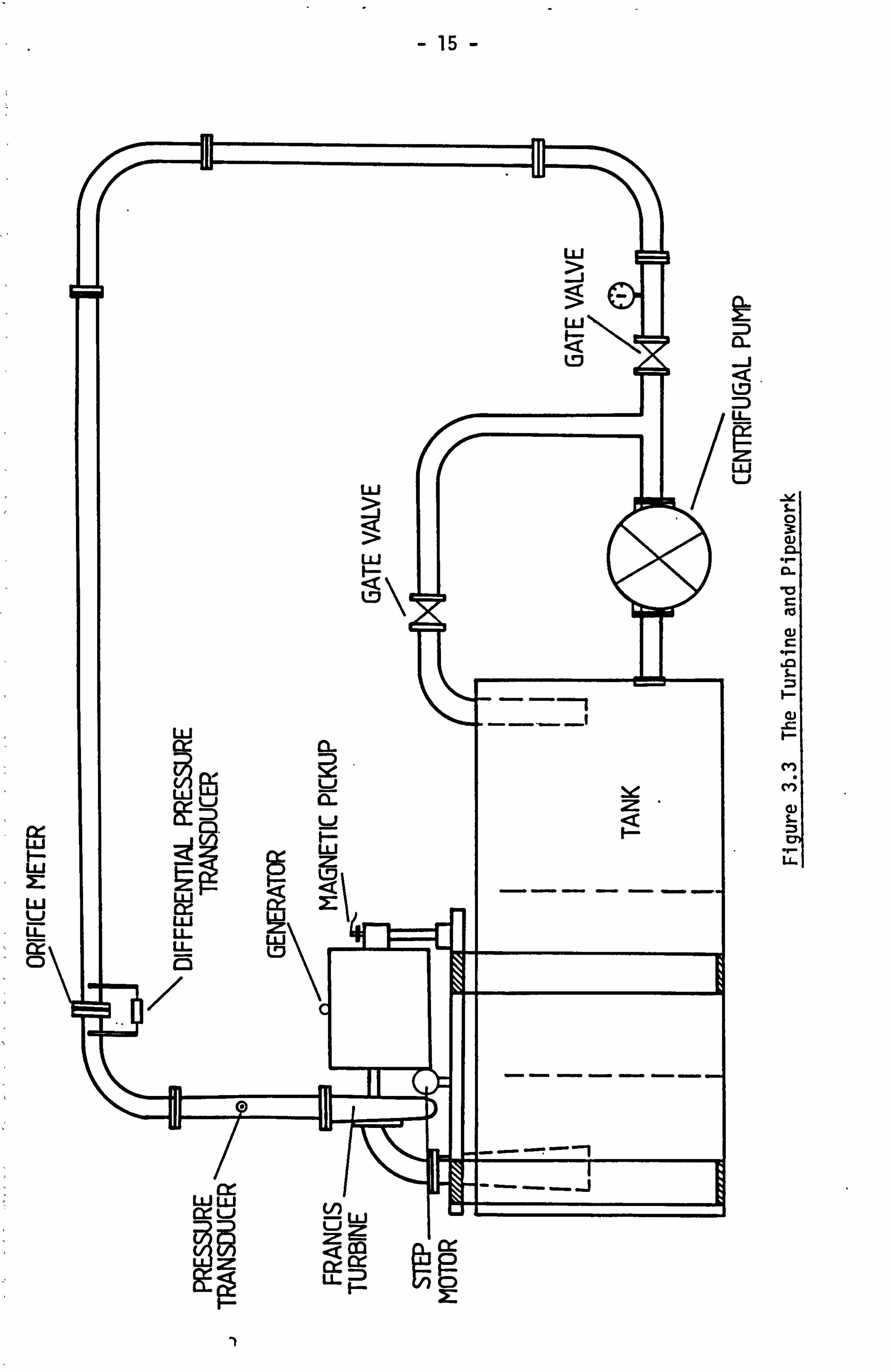
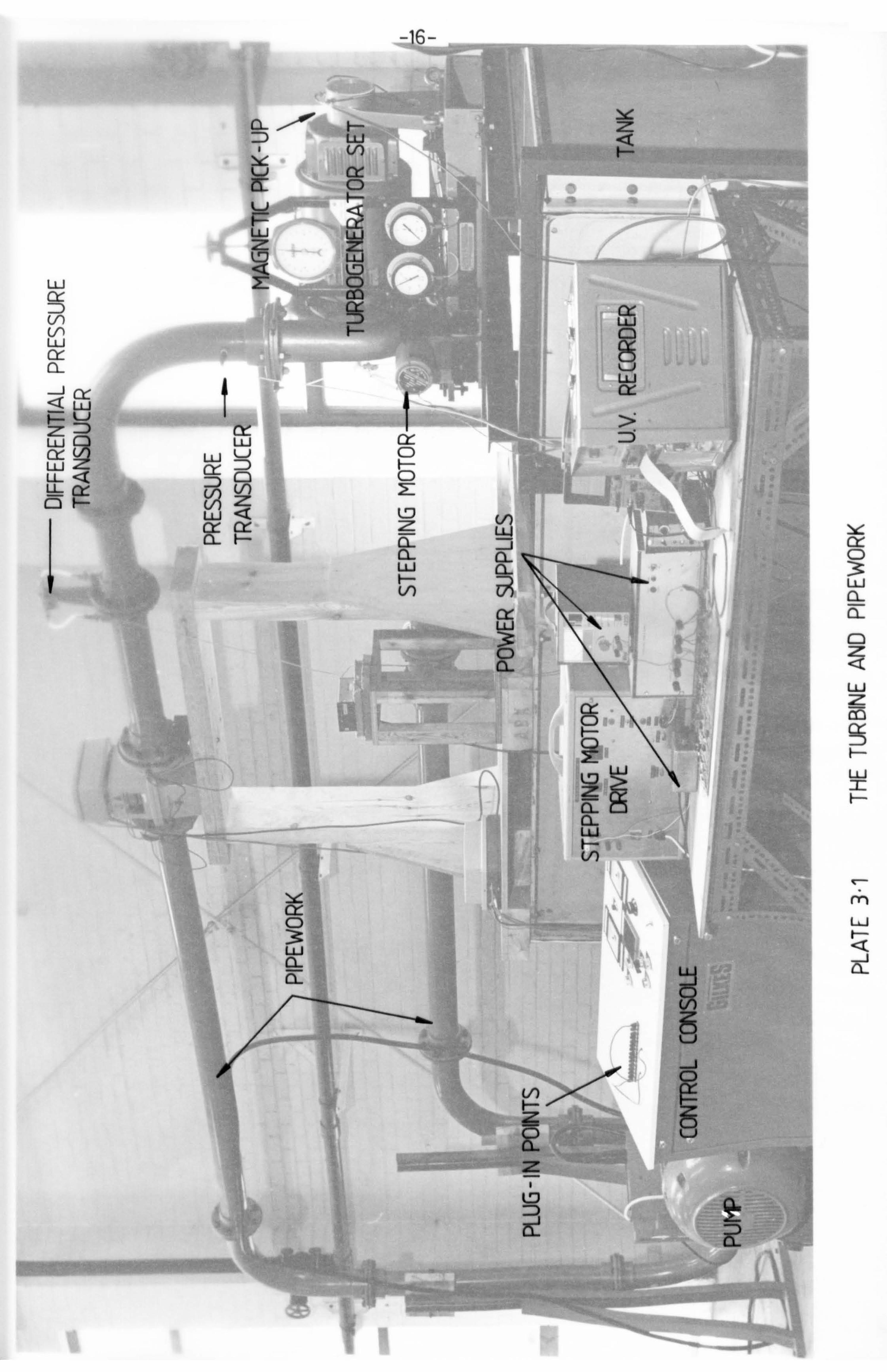
3.1 The Turbine and the Pipework 16

4.1 The Control Circuit 35 4.2 The Tachometer 57 4.3 The Stepping Motor and the Connected gears 60

NOMENCLATURE

a Waterhammer wave velocity (m/s) A Cross-sectional area of pipe (m2) D Pipe diameter (m) DR Turbine runner diameter (m) f Darcy-Weisbach friction factor

9 Acceleration due to gravity (m/S2 HA Piezometric head at beginning of time step at Ax from turbine

(m) Hn Net head (m) Hp Piezometric head at end of time step at turbine inlet (m) Ht Tailwater level above datum (m) I Moment of inertia of rotational parts (Kg m2) KD Gain of derivative element KE Voltage constant of step motor (volts/radian) KI Magnetic null displacement constant of step motor (radians/amp) Km Constant of analogue multiplier Kp Gain of proportional element n N/Nr N Rotational speed (rpm) Nr Rated speed (rpm) P9 Power of generator (KW) Pt Power of turbine (KW)

p Unit power q Unit flow QA Flow at beginning of time step at Ax from turbine (m 2/i)

Qe First estimate of Qp (m3/s) Qp Flow at the end of time step at. turbine inlet (m3/s)

R Resistance of step motor windings S Laplace Dperator TA Smoothing network time constant I'D Time constant of the derivative element T, Time constant

, of the integral element

Ts Time constant of step motor winding TU Unbalanced torque (Nm)

At Time step (s)

VA Smoothing network output

VD Output of derivative element VI Output of integral element VP Output of proportional element AX a At z Input to derivative, integral and proportional elements

ng. "

Generator efficiency

nti Turbine efficiency Permanent speed droop Unit speed

w Rotational speed (rads/s)

Total load moment of inertia referred to motor shaft Vr-T Damping ratio

-I-

CHAPTER 1

INTRODUCTION

1.1 GENERAL

Nearly all prime movers used in hydroelectric power systems are equipped with governors by means of which their speed can be controlled automatically. Recently the control of the proportional- integral-derivative governor for hydroelectric systems has achieved world wide interest because of its faster response, small size and higher accuracy and sensitivity than meclianital governors. In order to place the subject of this study within a somewhat more general frame-

work, the scheme of a hydroelectric power unit must first be explained.

1.2 GENERAL DESCRIPTION OF HYDROELECTRIC PLANTS

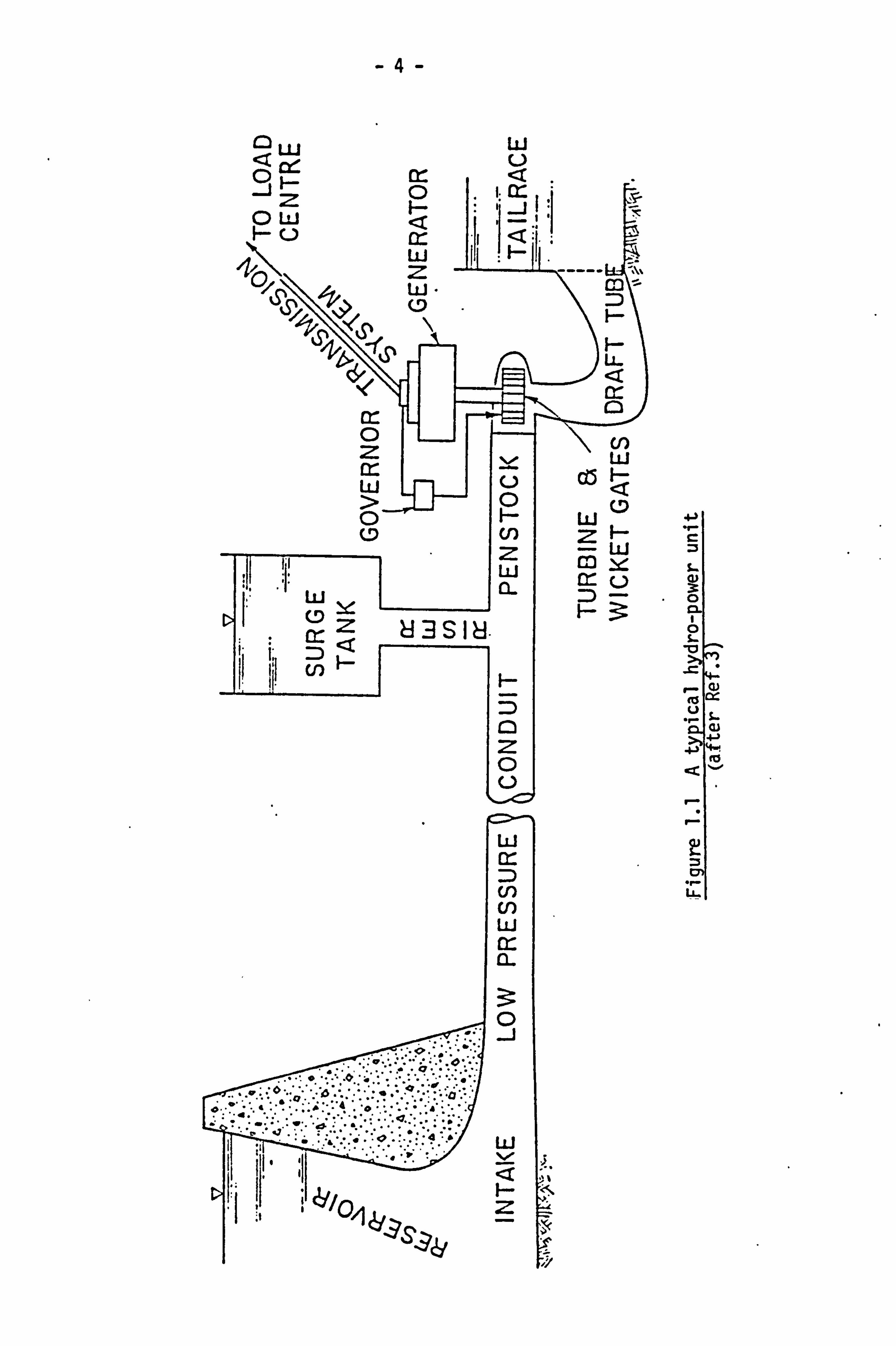
Figure 1.1 shows the interconnection of the principal elements of a typical hydroelectric installation with a simple surge tank.

The supply reservoir stores the water which is finally de- livered to the exhaust reservoir at lower elevation. The water flows from the supply reservoir to the surge tank through a supply line which may be either a free-flowing channel or a concrete aqueduct. The latter is generally called the conduit, while the supply line between

the surge tank and the turbine (which must withstand higher pressure than the conduit and is therefore constructed differently) is called the penstock.

The penstock delivers the flow to the turbine from the surge tank, either as shown in the Figure or, in the case of concentrated fall (no surge tank), installations, directly from the supply reservoir. The wicket qates, or movable vanes, act as structural modulators of the turbine water consumption and thereby determine the generated power. The turbine transduces the fluid power of the supply stream to mechanical power which islin turn transduced to electrical power by the

generator. The water, having spent much of its available energy, is

exhausted through the draft tub into the tailrace.

-2-

1.3 NATURE OF THE TRANSIENTS PROBLEM

Change in the power demand of the load centre served by a hydroelectric power system initiates a period of complex unsteady behaviour the effects of which are transmitted to every part of the

system from the load centre through the transmission system and into the various mechanical and hydraulic components of the power plants. The transients problem may be characterized by the following chain of interrelated events: the load change propagates over the transmission line (Figure 1.1), to the generator resulting in modification of the

electrical resisting torque seen by the generator rotor; this results in an unbalanced torque on the turbine-generator unit which causes a change in the rotational speed of the unit; the speed variation acti- vates the governor which alters the turbine gate opening; the changed gate position alters the amount of discharge through the gate thus initiating unsteady effects in the hydraulic system which appear as level changes in the surge tank and as rapidly propagated pressure fluctuations; these affect the turbine head and discharge thus pro- ducing new speed variatioýs whichs in turn, initiate a new sequence of transient effects throughout the entire system. At all stages of the

process, reflection and dispersion of the propagating quantities and damping (electrical, mechanical and hydraulic), create interactions

and forces which greatly complicate the process but which, in properly designed systems, limit the magnitude of the transient effects and pre- vent an unstable response to the load changes from occurring. It is

the task of the designer to ensure that the magnitudes of these effects are kept within acceptable limits and that unstable response cannot occur under any possible load change conditions. &

1.4 THE PRESENT WORK

1.4.1 Objective

The objective of this work can be summarized in the following

poi nts:

(a) To develop a computer program using an improved interpolation technique to deal with the turbine

-3-

boundary conditions making use of piecewise Lagrangean interpolation.

(b) To design and build a proportional plus in-

tegral plus derivative (PID) governor to

control a small turbine installed in the laboratory.

(c) To study the stability of a MD governor using a Bode plot method.

1.4.2 Layout of this work I

In Chapter I the nature of the transients problem and a scheme of ý hydroelectric power plant has been described.

Chapter 2 contains a reyiew of the works of others which is

of particular releyance to this thesis.

In Chapter 3 the mathematical representation of the system and the derivation of the boundary conditions has been explained. Also a general explanation of Lagrangean interpolation technique and the derivation of the Lagrangean interpolation equations and the

advantages and accuracy of this type of interpolation has been explained.

Chapter 4 explains'the rig and the design of the proportional- integral-derivative governor. Also the stability limit of the governor has been found making use of the Bode plot method. All the instru-

rents used are described together with an estimate of their accuracy.

Chapter 5 contains the description of the computer program and the computational procedure. A flow chart for each part of the

program and the main program has been drawn.

Chapter 6 describes a comparison between the computational and experimental results and presents a plot for each test.

Chapter 7 contains the conclusions of the thesis and some suggestions for further work.

-4-

LLJ < c): f Ld u

01-- z

w 0

< 1. cr-

0 Ld < ir- w

z w- (D

0 z It %. ooo w >

C) 0

U) z w

* LLI

O 0-

Z <

83SI8. M) cn

z 0 0

LLJ

U) LLJ m 12-

tu i I-

I c! //O, i

1--

F- U-

LU

LU

w c3 ir- u

. 4) "1

0

r-

I-

LL

-5-

CHAPTER 2

LITERATURE REVIEW

2.1 COMPUTATIONAL METHODS

Investigation of transients caused by governed hydraulic turbines began with the advent of the turbines and Control Systems. Early methods of computation are well covered by C. Jaeger in his book "Engineering Fluid Mechanics" (Ref. 1).

Swiecicki (Ref. 2), 1961, investigated the regulation characteristics of a hydraulic turbine by using a step-by-step arithmetical integration. Equations weredeveloped to calculate speed and pressure transients of a hydraulic turbine during a load change. A computer program was developed- (Ref. 3), in which the dynamic and continuity equations were solved by an implicit finite-difference method. The turbine characteristics were included in a simplified form and the

governor was represented by a linear third-order ordinary differential

equation having constant coefficients i. e. the saturation of various elements was not included. Wozniak and Fett. (Ref. 4) developed a computer program for closed-loop simulation of the transient behaviour

of a hydroelectric power plant. In this program the governor nonlinearities were included and the conduits were represented by a Mac- laurin series expansion of the closed-form solution of the linearized

partial differential equations. Streeter and Wylie (Ref. 5). presented a mathematical model in which a method of characteristics was used to simulate the conduit. Turbine characteristics were included

and the governor was represented by a second-order ordinary differential equation. Chaudhry (Ref. 6) presented another mathematical model in which turbine characteristics were globally represented. A method of characteristics was used to solve the continuity and dynamic equations representing-transient flow in closed conduits. A temporary-droop governor was represented by five first-

order differential equations and all major nonlinearities of the

governor were included. Two iteration loops were required to solve the equations. In another computer program (Ref. 7), the number of iteration loops were reduced to one by combining the equation of the

-6-

instantaneous speed change with equations of the governor and a solution was obtained by the fourth-order Runge-Kutta method. The finite difference method was used in dealing with turbine characteristics.

2.2 GOVERNING STABILITY

The speed oscillations of a turbogenerator in a hydroelectric

power system are caused by load change. To control these oscillations a temporary droop governor or a PID (Proportional, Integral, Derivative)

governor is usually provided. These oscillations may be either stable or unstable depending on the value of the parameters which are the tem-

porary speed droop and the dashpot time constant in a temporary droop

governor and the proportional, integral and derivative gains in a PID

governor.

Paynter (Ref. 8). presented a stability limit curve and sug- gested optimum values of the governor settings by solving the problem on an analogue computer. Hovey.,, (Ref. 9). derived a similar stability curve theoretically, i. e. the differential equations of the system were derived with the main parameters involved in the speed transient of the turbine following a load change. All non linear relationships were assumed to be linear and he applied his analysis to a practical power system. The work of Paynter and Hovey, which treated the case of a temporary droop govemor, neglected the following factors: -

(1) The steady state speed droop. (2) The net damping torque. (3) The mechanical inertia of the rotating leads.

Chaudhry (Ref. 10) extended the work of Hovey to include

the effects of gate feed-back and self-regulation. His work shows that the stability boundaries are greatly extended when these factors

are included. Hovey and Chaudhry established the stability boundaries by first setting up a third order differential equation in speed and then applying the Routh-Hurwitz criterion.

Thorne and Hill. (Ref. 11) were the first to apply the

state-space approach to the study of PID governors and examined the

-7-

stability boundary as a function of proportional gain, integral gain, system damping and turbine loading. Furthermore, an operating boundary is derived from the time-response requirements of the governor. Thorne and Hill's work was undertaken with the following limiting conditions: -

The unit steady state speed regulation was set at zero.

(2) The remaining equivalent system operated with a blocked governor.

(3) No account was taken of the derivative gain effect on stability.

(4) No effect of interconnection to neighbouring utilities was considered.

Dhaliwal and Wichert (Ref. 121 also used the state-space approach to study PID governors in a multi-machine system in isolated operation. While the effect of governor derivative gain on the stability was considered, no stability boundary was defined. Their work used an ideal simplified relationship between mechanical torque and gate opening and neglected damping torque due to the prime mover and generator. A high derivative gain can cause the system to go unstable.

The works of Hovey and Chaudhry are expanded to show the stability boundaries of a hydraulic turbine generating unit having a PID

governor by Hagihara et al (Ref. 13). They established the stability boundaries by setting up a fourth order differential equation in speed and then applying the Routh-Hurwitz criterion. The effect of de-

rivative gain was studied, not directly but through the intermediary

of a parameter that also implicates the proportional gain and the water start time. Hagihara et al used an ideal simplified model of the hydraulic conduit, i. e. the relationship between mechanical torque and gate.

D. T. Phi et al (Ref. 14) investigated the incident of unstable frequency oscillation that occurred on March, 1977, following a major system disturbance on the New Brunswick power system. Their

-8-

work was extended and complemented by other authors (Refs. 10-13). taking into account more parameters and more varied operating conditions.

-9-

CHAPTER 3

THEORETICAL ANALYSIS

In this Chapter the mathematical representation of the system is based largely on Chaudhry (Refs. 6,7) with the exception of the

method of dealing with the boundary conditions.

3.1 TURBINE AND THE CONDUIT SYSTEM

3.1.1 Representation of the Conduit

The method of characteristics and the boundary conditions presented in the standard manner, (Ref. 6), was used to analyse the pipework system.

In the method of characteristics the partial differential

equations are converted into ordinary differential equations which are then solved by finite-difference technique. A summary of the necessary equations is given below, for details see Ref. 6.

For an intermediate section of a pipework:

QPI = 0.5 (ýp + Cd (3.1)

HP, = 0.5 ( Cp

ca Cn

(3.2)

in which

cp = fAt (3.3) QI-I "' Ca'I-I MT QI-I/QI-I/

cH fAt (3.4) ný QI+l - Ca I+l - 79 QI+1'QI+ll

c gA (3.5) aa

- 10 -

For the upstream end

QPI 7-- Cn + Ca Hp, (3.6)

For the downstream end

QPn+l "- Cp -CaH Pn+l (3.7)

In the above equations, Q is the transient flow, a is the pressure wave speed, At is the time-step chosen for the calculation, A is the cross-sectional area of the pipe, D is its diameter, f is its friction factor, H is the piezometric head, subscript PI indicates conditions at Section I at the end of a time-step and the subscripts I, I-1, I+l denote conditions at these ptpe sections at the beginning of a time-step.

The unknown flowrate and piezometric head at point I are ex- pressed in terms of their known values at points I+l and I-1.

3.1.2 Representation of tKe turbine

The relationship between the net head and discharge has to be

specified to simulate a turbine in a hydraulic transient model. Flow through a turbine depends upon various parameters: for example, the flow through a Francis turbine depends upon the net head, rotational speed of the unit and wicket gate opening. Curves representing the

relationship between these parameters are called turbine characteristics. These curves are obtained from tests conducted on the model of the turbine runner.

The characteristic curves for the turbine used in the laboratory

are shown in Figures 3.1 and 3.2. In these Figures, the abcissae are the unit speed, 0, and the ordinates are the unit flow q, and the unit power, p. Definitions of 0, q and p used are: -

DRN Unit speed ý=. ý-- (3.8)

8 4.4 5 YITN-

- 12 -

- 12 -

Unit flow qp (3.9) D RN

Unit power p= -2 t. 31Z DRN

In these definitions DR is-the turbine runner diameter, N is the rotational speed, HN is the net head, Qp is the flowrate at the turbine, and Pt the power of the turbine.

A grid of points on the characteristic curves for various gate openings was stored in the computer and the unit flow, unit power and unit speed at intermediate gate opening were determined by using Bivariate Lagrangean interpolation.

3.1.3 Turbine-Generator Torque Equation

The speed of the turbogenerator set increased due to unbalanced torque CTu) after load reduction such that: -

Tu =I du rt (3.111

in which I is the moment of inertia of the rotating parts of the turbo-

generator set and w is the rotational speed of the unit in radians/s. Equation (3.11) may be wri'tten as: -

p dw L2 =I" -31 n9c

Hence dn 91.19 (P C3.13) HE 2-t INRn

in which Pg is the final generator load, n- NINR and NR is the synchronous speed.

In equation (3.13) there are two unknowns n, Pt and we need another equation for a unique solution. This equation is provided as fol I ows.

- 14 -

The characteristics for unit power (p) for a particular gate opening (T) may be approximated by a parabola over a small speed range, so

C0+C10+C 20 2

where COXI and C2 can be determined by Lagrangean interpolation.

Using equations (3.8) and (3.10) into equation (3.14)

pt =a7+a8n+a9 n2

where a=CD2H1.5 70RN

CD3NH 184.45 1RRN

CD4N2A Y(84.45) 2 92RRN

i. e. equation (3.13) can be written as:

(3.14)

(3.15)

dn 91.19 2 ! 9)

IN2n (a 7+ an +a9n9

R

Hence equation (3.16) may be integrated by the fourth-order Runge-Kutta method CRef. 15), together with the equations of the goyernor giYen in the following section.

3.2 DERIVATION OF BOUNDARY CONDITIONS

The laboratory set up is shown in Figure 3.3 and Plate 3.1. Special boundary conditions are required to represent the conditions at the upstream and downstream ends of the system.

- 15 -

cr- LLJ

LLI Li Cc cr- C)

if

Q3

Li

. r- CL

M r_ (0

(Y)

c)

-r-

LL-

.Z (2: LL

CCP-2 ,Z

Ii

Qý CD CD

U. j F- V)

Q: LLJ 0 Fsj

L ItI

\o

cy- C) f R

C) LLJ a-

n M Iz LU 'Z

LLJ r,

F-

rT LJ 1-

Zý

i

U tV

1»

0 'd

: ýi

tiff

lt

- 17 -

3.2.1 Upstream_Boundary

The input to the system was supplied by a pump, but a large

pump with a by-pass was used so that a required combination of head and flow could be obtained without haying to match the pump characteristics. As shown below the relation between the pump, the conduit and the by-pass

was derived as follows.

GATE VALVE

PUMP 1234

PIPEWORK

I The relation between the head and the discharge of the

pump can be approximated by the equation

HP =c7- c8Q 2 p

(3.17)

2. The gate opening of the gate valve of the by-pass is constant for a given test so can be approximated by the equation

K Y'17pý s (3.18)

3. The inlet flow to the system is:

Qc = Qpump - Qby-pass

4. Equation for total head at point (1)

Hpump = Hby-pass- H1=Hp C3.20)

- 18 -

From equations (3.171 and C3.18) into equation (3.19) the flowrate at the inlet of the conduit is giyen by

K vffýýs

In the above equation C7 and C8 are the pump constants calculated from the pump characteristics, K the orifice constant for the

valve.

Equation (3.21) and the negative characteristic equation (3.6)

give two equations for two unknowns, i. e. the boundary conditions at the inlet are represented by these equations.

3.2.2 Downstream Conditions

To develop the boundary conditions for the turbine end, one has to solve the positive characteristic equation (3.7) with the relationship between the flow, Qp, and net head, HN, imposed by the boundary. The flow through a Francis turbine depends upon the head, HN, gate opening,

T, and the speed of the unit N. Since the gate is opened or closed under governor control depending upon the turbine speed which is also unknown, equations between these variables have to be solved simultaneously.

As shown in Ref. 6 the relationship between the inlet head of the turbine and the net head HN is:

Q2 HP =HN+RT-

2g A2 (3.22)

where HT Is tailwater level above datum.

The values of the four variables namely Qp, Hp, T, and N are

unknown at the end of each. time-step during load change and rAy be obtained by the following procedure.

- 19 -

The characteristics for unit flow (q) for a particular gate opening (T) can be approximated by a straight line oyer a small in- teryal of speed. The equation of the straight line may be written as:

a0+a 14, (3.23)

where ao and al can be determined by Lagrangean interpolation. Sub-

stituting q and ý from equations (3.8) and (3.9) into equation (3.23)

H, i=Q 2qp-a3 (3.24)

where aaD2 2 ý-- 0R

aN D2 a 184.45 3ýRI

From equations C3.7), (3.22) and (3.24) the flowrate at the inlet to the turbine is given by:

a5 -/a5 - 4a4a6 Qp 2 a4

where a= Ca](2 gA 2)

- Cala 2 42

a 2a C Ja2 53a2

aC-cHCa2 /a 2 6pata32

(3.25)

Using equation (3.25) Qp is found. By substituting into equations (3.24) and (3.22) HN and Hp are found, i. e. the boundary conditions at the inlet of the turbine are known.

As discussed before the boundary conditions at the boundaries

are known so we can find the conditions at time t= At.

To illustrate how to use the previous equations (3.1), C3.2), C3.61 and (3.7) the pipework is divided into n equal reaches and the

- 20 -

steady state conditions at t= to are first obtained. Then, to deter-

mine the conditions at t= to + at, equations (3.1) and (3.2) are used for the interior points and the boundary conditions at the upstream and downstream together with equations C3.61 and C3.7) are used to calculate the conditions at the end of the time-step. Now conditions at t= to+ At are known and the conditions at t- to + 2, &-t are determined by following the same procedure. In this manner, the computations proceed step-by- step until transient conditions for the required time are determined.

3.3 PROPORTIONAL-INTEGRAL-DERIVATIVE GOVERNOR

3.3.1 General

The governor is provided to keep the speed of the turbo-gene-

rator at the synchronous speed.

There are three types of goyernors used for hydraulic units.

(1) Dashpot governor (2) Accelerometric governor (3) Proportional-Integral-Deriyative governor (PID).

The dashpot governor has been more commonly used in North America and the accelerometric in Europe, the PID has been introduced during the last ten years. In the dashpot governor the corrective action of the governor is proportional to the speed deviation, An; in the accelerometric governor it is proportional to dnldt; in the PID it is proportional to An; dn]dt and time integral of An.

3.3.2 Representation of the Governor

As shown in the block diagram, Figure 3.4, the governor components are:

3.3.2.1 Phase-locked loop

A phase-locked loop contains three basic components as shown bel ow:

(L

b 2 a- LU

ir

w

Z

u) + f\+

+

(N w V) > C14

tn 51 C3 + V)

w CL

- 21 -

5 N

CN

IL 0 0

ie

b

S- o

4- 0 P

u 0

cl;

cr . I- Lj-

- 22 -

Cl) A phase detector CPDJ (2) A low-pass filter C3) A voltage-controlled oscillator (YCO) whose frequency

is controlled by an external voltage.

PD

S

The phase detector compares the phase of a periodic input signal against the phase of the VCO; the output of the PD is a measure of the

phase difference between its two inputs. The difference in voltage is then filtered by the loop filter and applied to the VCO. Control

voltage on the VCO changes the frequency in a direction that reduces the

phase difference between the input signal and the local oscillator.

As shown in Figure 3.4 the input signal is

Vin :-A Sin w, t where Vin -n (3.26)

The output signal is:

Vout =A1 Sin w2t where V out "' nref (3.27)

where A is the amplitude of the input signal and proportional to the speed of the shaft.

A, is the output amplitude of the phase-locked loop, it is a constant.

Basic Phase-loc. ked Loop

- 23 -

The aim of PLL

1. To ensure that q and u)2 are in the same phase and are equal.

2. To generate a constant amplitude to represent the

reference speed (bias voltage) at the input of the analogue multiplier while generating an error signal to control the system operation.

3.3.2.2 Analogue multiplier

The main function of the multiplier is to compare the reference voltage which represents the reference speed (nref) and the variable voltage which is proportional to the speed (n).

v out = A, Sin uýt (3.27)

and V in(multiplier) =A Sin w, t (3.28)

Due to the feedback V in(multiplier) ,, n+ aT

But wl ý w2 due to PLL

v in(multiplier) cA1 Sin w2t

v in(multiplier)* v out ýA Al(Sin wt)

2

LAA+A Al Cos 2wt (3.29) ýl z

The output of the multiplier = Km-Vin(multiplier). Vout and

Vin'Vout , nref (n+oT)

Note: If Al A the output signal is negative If Al A the output signal is positive

i. e. the sign (t) dictates the direction of the turbine gate.

3.3.2.3 Controller

(i) Proportional

The proportional mode of control is very widely used by itself and also in conjunction with other modes which are added to obtain

- 24 -

certain performance improvements. The proportional element is as follows:

Let

Then

Kmn ref*

(n+CT) (-3.30)

Vp =

where Z= output of the analogue multiplier Kp = the gain of the proportional element vP= the output of the proportional element.

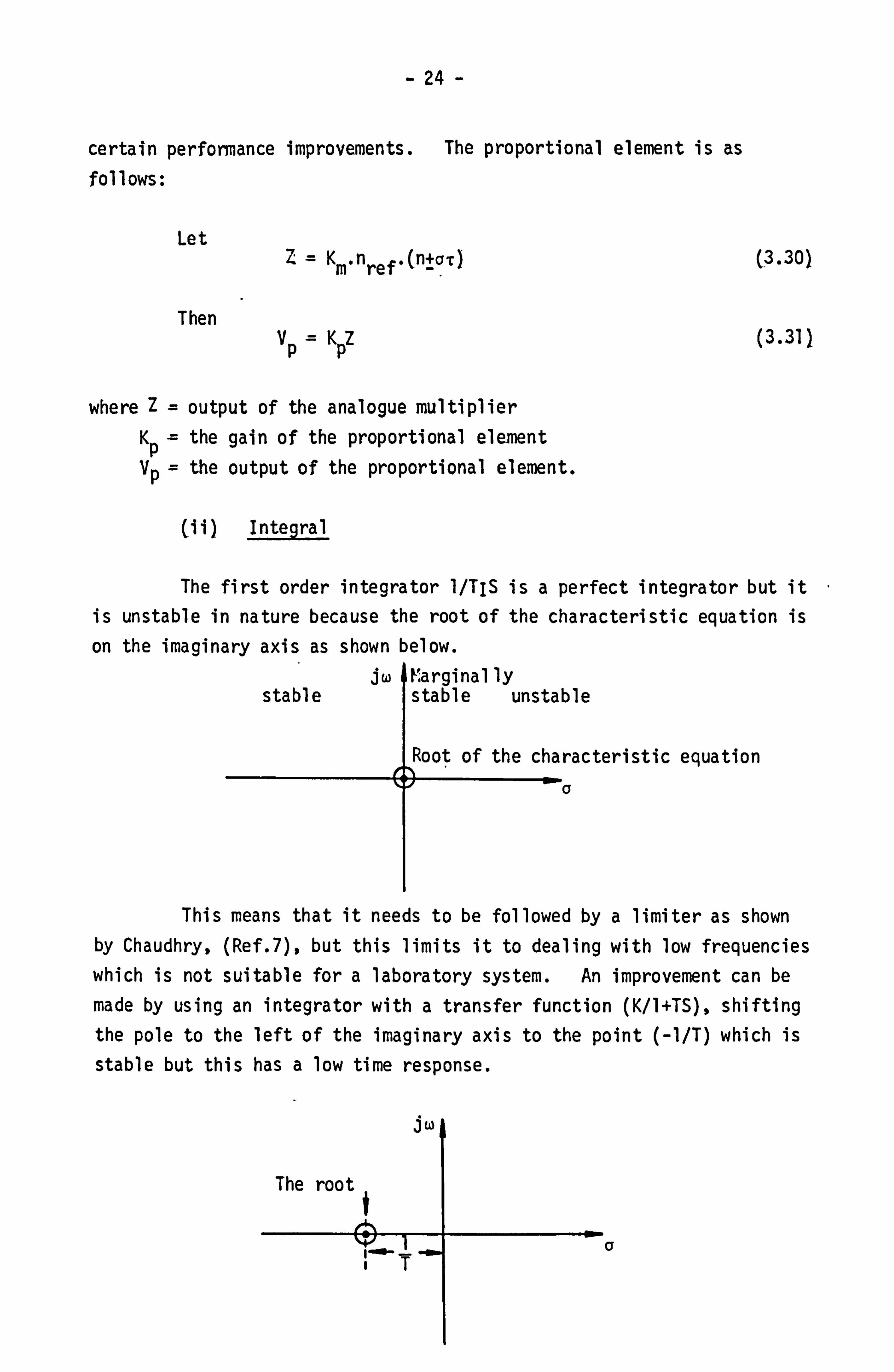
(ii) Integral

(3.31)

The first order integrator I/TJS is a perfect integrator but it is unstable in nature because the root of the characteristic equation is

on the imaginary axis as shown below. jw Marginal ly

stable Istable

unstable

Root of the characteristic equation a

This means that it needs to be followed by a limiter as shown by Chaudhry, (Ref. 7), but this limits it to dealing with low frequencies

which is not suitable for a laboratory system. An improvement can be

made by using an integrator with a transfer function (K/I+TS), shifting the pole to the left of the imaginary axis to the point (-I/T) which is

stable but this has a low time response.

a

- 24(a) -

TQ improve this response o, second order system. can be designed to give faster respQnse with lowest overshoot transilent response as shown below.

step pulse

transient resDonse stea ,. -- 1 lst Order 1

17 is

ksetting

time 1

transient 2nd Order responsel steady state

1+2T S+T2S2

setti ng time

state

Appendix A shows the derivation and design of the second order integrator, i. e. the transfer function becomes:

VI(s) -12Z (3.32) 7-(ýy 1+ 2T IS+TIS

where S= Laplace operator which is equivalent to d/dt if the initial

conditions are zero.

Then d2v lz

-v 2T dV 1 (3.33)

dtT 7 -t A

- 25 -

where VI is the output of the integral element and Tj is its time constant.

(iii) Derivative

The differentiator should be compatible with-the integrator

and hence a second order differentiator was also used. This differentiator can be designed in two forms:

KDs2zz

+TDS+TDs

(b) KDsz7

1+ 2T DS+TDs

It was found that the first had got a limited gain but the

second had unlimited gain which improved the dynamics of the system. The transfer function of the derivative elements may be written.

v D(S) KDs

(3.34) - T, -17z-ý7 ZTIS I+ 2TDS + TBS

Then by substituting S= djdt

d2 VD =

17 IK

D dZ

- 2T D dVD

_ VD (3.35) dtT- - 3t TD

where VD is the output of the derivative element KD is its gain and TD is its time constant.

3.3.2.4 Smoothing network

Practically the output of the controller is DC plus AC (low

frequency). To filter this frequency a smoothing network is introduced

to give approximated DC input to the actuator.

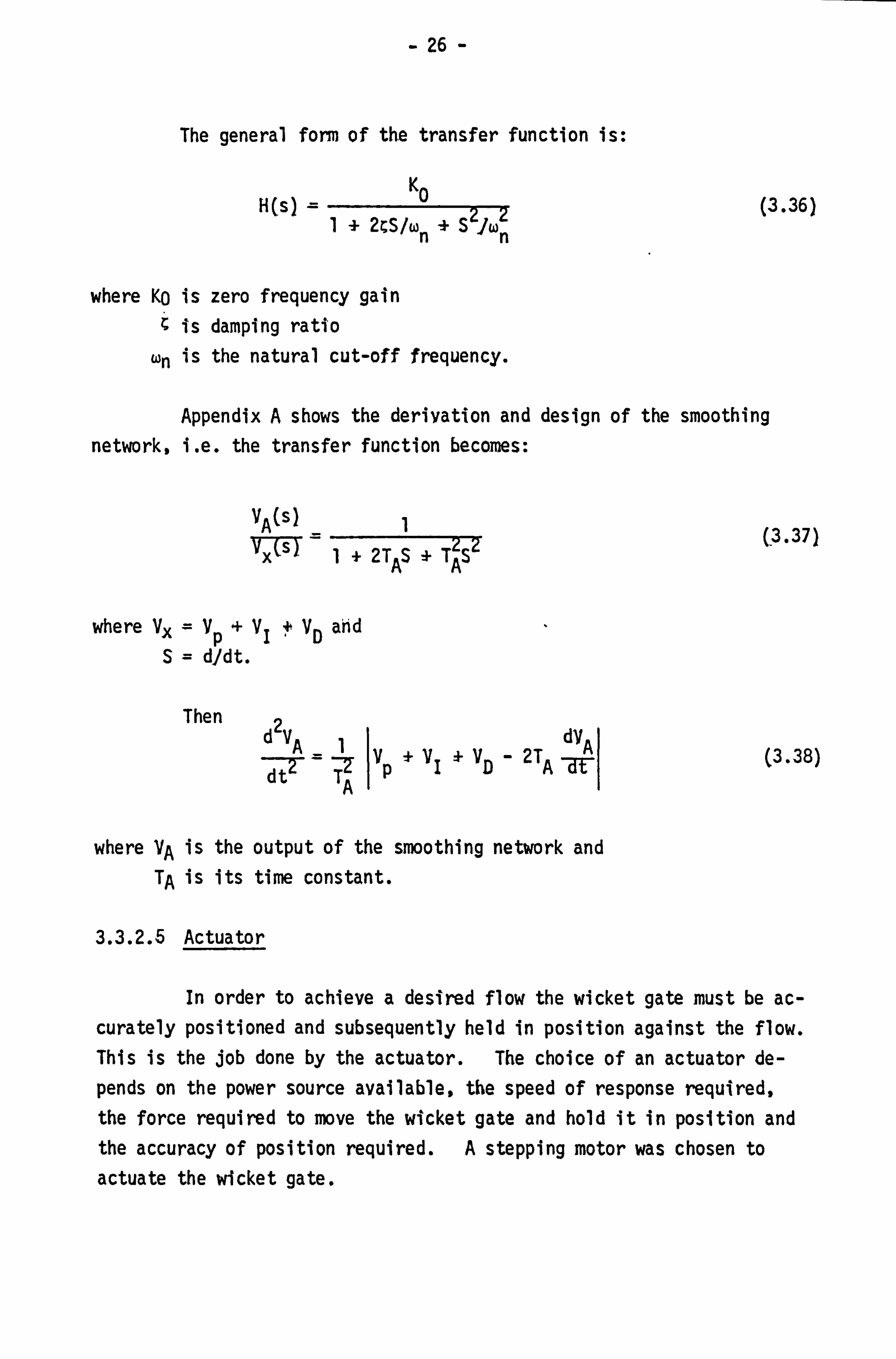
- 26 -

The general form of the transfer function is:

ZIwz I+ M/w n+Sn

where KO is zero frequency gain is damping rati, o

wn is the natural cut-off frequency.

(3.36)

Appendix A shows the derivation and design of the smoothing network, i. e. the transfer function becomes:

VA(sl T 'T X-T sI+ 2TAS +T AS2

where Vx =Vp+vIý VD ahd S= dIdt.

Then d2vA JVP W T7. A

V+v- 2T dV AI

IDA -aY

(ý. 37)

(3.38)

where VA is the output of the smoothing network and TA is its time constant.

3.3.2.5 Actuator

In order to achieve a desired flow the wicket gate must be ac- curately positioned and subsequently held in position against the flow. This is the job done by the actuator. The choice of an actuator de-

pends on the power source available, the speed of response required, the force required to move the wicket gate and hold it in position and the accuracy of position required. A stepping motor was chosen to

actuate the wicket gate.

- 27 -

Step motor

For electric motors to generate the required power economically the rotational speed of the motor is high, the high speed low torque is

converted to low speed high torque by gearing. This had advantages in

an infrequent on/off operation where an impact hammer blow may be required to move the gate off its seat. It is though, a disadvantage in the control loop where the momentum will cause overrun from the desired

position.

One type of electric motor which does not suffer from the problem of overrun is the DC stepping motor. This motor remains static

when energised. Movement is caused by de-energising and then re- energising the stator windings in a different pattern. This sequence is controlled by drive circuitry which changes the pattern following

receipt of an external pulse. The power output of a DC stepping motor is limited. One advantage which the electric motor does possess in

the control loop situation, is high stiffness. That means the movement of the gate under dynamic loading resulting from pressure fluctuations in the flow is small.

Theoretical transfer function

Delgado, (Ref. 16), assumed the self inductances were constant and the inertial torque included the applied torque. He also assumed there was no mutual inductance between stator phase windings. The induced voltage was assumed to be a linear function of speed and the resulting equation was a linear third order system.

T(S) =Nc (3.39) TATST AS3 + BS2 +McS+I

where A=J Ts/Kr B= J/Kr

Mc = Ts +(KE-KI/R) Nc = KI/R Kr = Restoring torque constant (N. B. usually Kr is very high) j= Total load moment of inertia referred to motor shaft.

- 28 -

Practically, A and B were very small so as to simplify the transfer function

Then

-r(s) Nc

(3.40) mc Zo *I

dT =I 'VA - TI a, - y-

IN c c

3.4 BIVARIATE LAGRANGEAN INTERPOLATION

3.4.1 General

Many contributions towards representation of turbine characteristics have been published within the last few years. Wozniak, (Ref. 19), used the least squares nethod. The turbine characteristics were globally represented by Chaudhry, (Ref. 7), who used finite difference interpolation.

The use of Lagrangean polynomials, (Ref. 17) is amongst the simplest and most practical methods of interpolation. The general equations of Lagrangean interpolation which are used in this work are as follows:

nmn (X) 9 (Y) zi, i 11

z 3.4.2 Derivation

V

xi X2 X3 Xi Xm

- 29 -

Along any y line which intersects line x=xi in point z(xi, y) using one dimensional interpolation along x=xi line.

nn z(xi SY) =I -t (Y)

J=j j

Applying the same one dimensional interpolation on y line

mm z(x, y) =i-, (A Z(xi, y) i=I i

Substituting equation (3.421 into equation (3.43) we get:

m

z(x, y) =i n m

x (X) n Z (Y) Z ij

The first and second partial deriyative of equation (3.44)

will giye the following equations:

m la

i (4) Dz 1

ax ZX zi

2m maxnn ZZm,

-i x)

i äxz i=i ul i=l jZ

whe re nm X-x r Z (x) = ii

r=I xi-xr ri i

(3.42)

(3.43)

(3.44)

(3.45)

(. 3.46)

From (Ref. 18) it can be proved that the errorobtained from the following fomula is

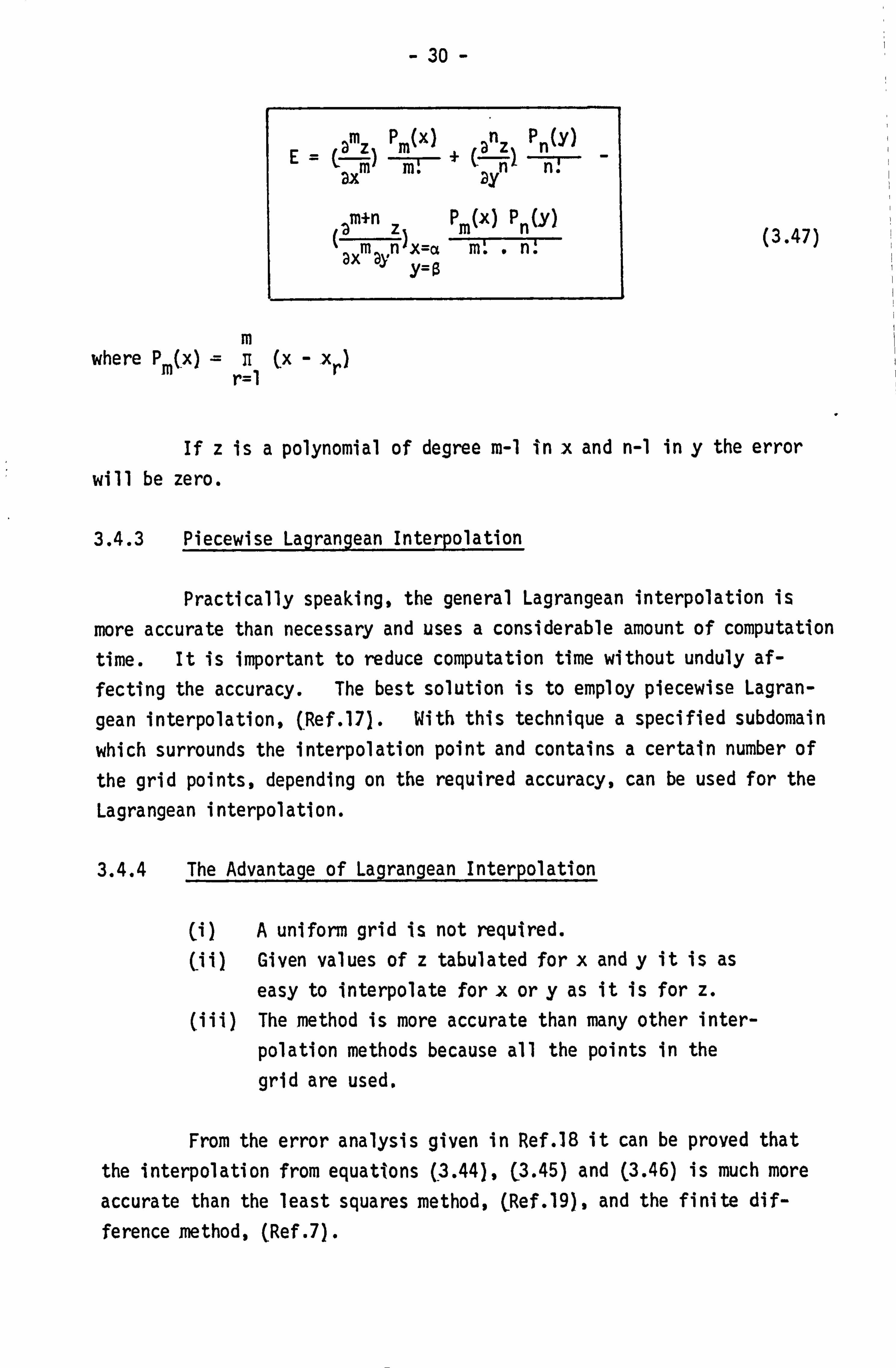
- 30 -

mp m(X) anz Pn(Y) 0 -mz

) -m-m- T. -+ (l- -i1 -n

ax zy

PM (x) Pn (y) (axmayn)x=a

m. . n! Y=ß

where Pm (x)- H (X -x r) r=l

(3.47)

If z is a polynomial of degree m-1 in x and n-1 in y the error

will be zero.

3.4.3 Piecewise Lagrangean Interpolation

Practically speaking, the general Lagrangean interpolation is

more accurate than necessary and uses a considerable amount of computation time. It is important to reduce computation time without unduly affecting the accuracy. The best solution is to employ piecewise Lagran-

gean interpolation, (Ref. 17). With this technique a specified subdomain

which surrounds the interpolation point and contains a certain number of the grid points, depending on the required accuracy, can be used for the Lagrangean interpolation.

3.4.4 The Advantage of Lagrangean Interpolation

(i) A uniform grid is not required. Cii) Given values of z tabulated for x and y it is as

easy to interpolate for x or y as it is for z. (iii) The method is more accurate than many other inter-

polation methods because all the points in the

grid are used.

From the error analysis given in Ref-18 it can be proved that the interpolation from equations (ý. 44), C3.45) and (3.46) is much more accurate than the least squares method, CRef. 19), and the finite difference method, (Ref. 7).

- 31 -

Piecewise Lagra, ngean interpolation has the following

advantages. (a) It saves computer time. (b) It my even improve the accuracy by reducing

rounding off errors, assuming a sufficient number of points has been used.

CC) Using a large number of values of T (gate

openingl will give greater accuracy without affecting the computer time.

- 32 -

CHAPTER 4

EXPERIMENTAL PROCEDURE

4.1 DESCRIPTION OF THE RIG

In order to carry out a series of tests a flow rig was built

in the laboratory using 100 mm ID pipes. These tests were for a range of partial load rejections as well as for full load rejection. A

plastic tube (ABS-durapipe) was used for the construction of the rig whose elements are explained below. A photograph of the rig is shown in Plate 3.1 and a diagram in Figure 3.3.

I. Pump

The input to the system was supplied by a large centrifugal pump, (Head = 29 (m), Q= 50 1/s, N=1,450 rpm, HP = 22 KW). A large

pump with a by-pass was used so that a required combination of head and flow could be obtained without having to match the pump characteristic to the system .

2. Valves

The water was controlled by two manual gate valves (100 mm diameter), one at the input of the conduit and another at the by-pass to obtain the required conditions of head and flowrate.

3. Tank

The tank which was made of plastic material was of about 3.5 m3 capacity. The turbogenerator set was fitted on the tank with a suitable frame, thus the draft tube was immersed in the tank.

4. Turbine and generator

A Gilkes 150 mm Reversible Francis pump/turbine was used. As-'a Francis turbine the machine has a high efficiency (73%) and test results can be repeated without difficulty. The 150 mm pump-turbine is integrally constructed with a dynamometer type motor generator.

ABSTRACT

This work is concerned with transients caused by changes in load on a turbogenerator set governed by a proportional plus integral

plus derivative (PID) governor.

A PID governor was designed and built in the laboratory to

control a small turbine installed in the laboratory. Having the turbine available in the laboratory meqnt that a full set of tests could be carried out for a range of partial load rejections as well as for full load rejection. A computer program was developed using an im-

proved interpolation technique to deal with the turbine boundary conditions making use of piecewise Lagrangean interpolation. The gate opening, turbine speed, pressure rise, and flow rate recorded in the laboratory are presented and compared with theoretical results from the computer analysis.

There is a good measure of agreement between the experiment and computed results, particularly up to the peak of speed and pressure rise.

- 33 -

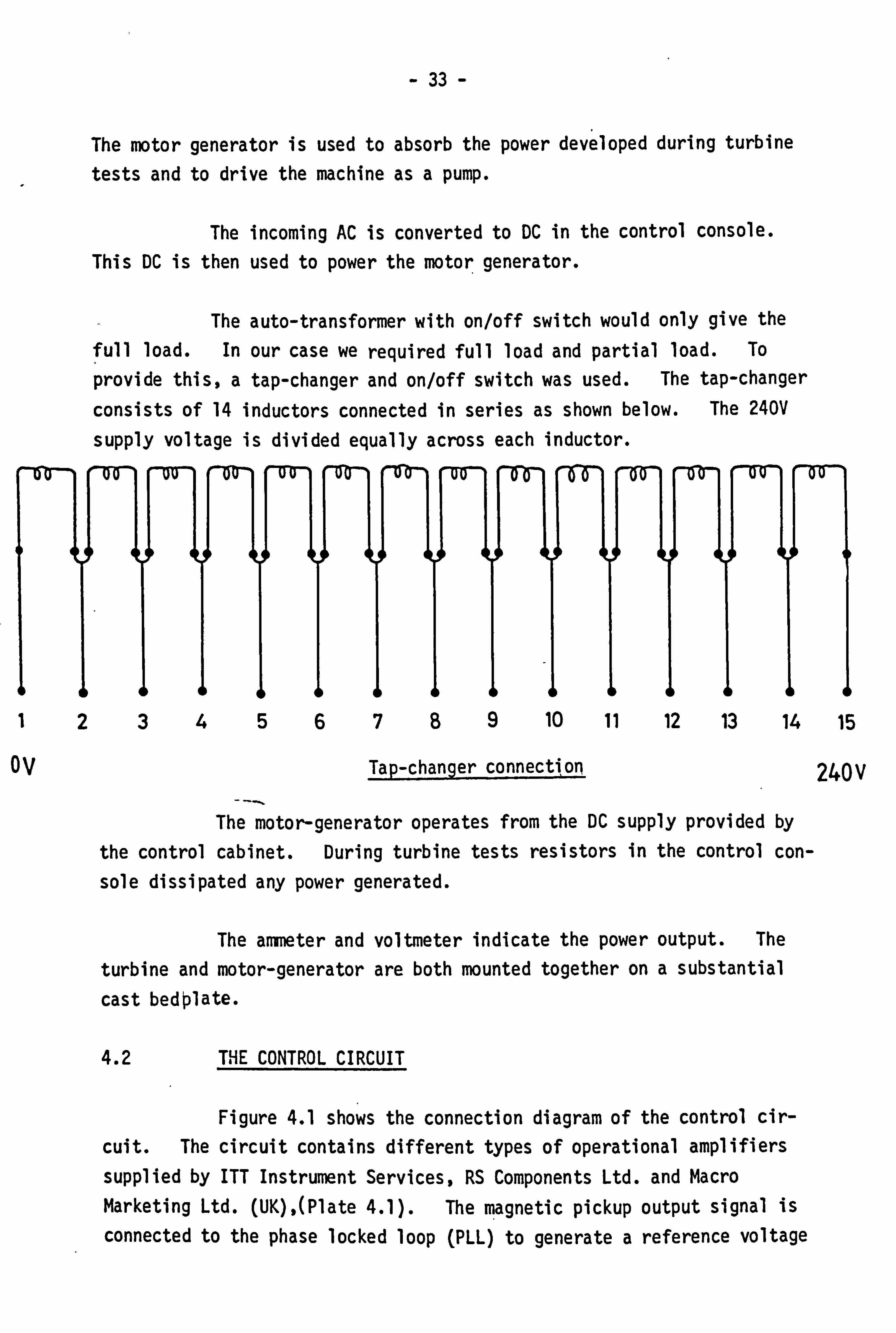
1

The motor generator is used to absorb the power developed during turbine

tests and to drive the machine as a pump.

The incoming AC is converted to DC in the control console. This DC is then used to power the motor generator.

The auto-transformer with on/off switch would only give the full load. In our case we required full load and partial load. To

provide this, a tap-changer and on/off switch was used. The tap-changer

consists of 14 inductors connected in series as shown below. The 240V

supply voltage is divided equally across each inductor.

10 11 12 13 14 15

ov Tap-changer connectlon 240V

The motor-generator operates from the DC supply provided by

the control cabinet. During turbine tests resistors in the control console dissipated any power generated.

The ammeter and voltmeter indicate the power output. The

turbine and motor-generator are both mounted together on a substantial

cast bedolate.

4.2 THE CONTROL CIRCUIT

Figure 4.1 shows the connection diagram of the control circuit. The circuit contains different types of operational amplifiers supplied by ITT Instrument Services, RS Components Ltd. and Macro Marketing Ltd. (UK), (Plate 4.1). The magnetic pickup output signal is

connected to the phase locked loop (PLL) to generate a reference voltage

I

t, )ý 34

12

i RX 15- >

>> cc 8 > cn in 0

co cn _j

co 0: ukI

ix

x ct

co co CP

>>>> LC) >>

Ln tri Ln tn z4 z>

S2 to AM cn S. -

co

C-4 -3 ul CD yj cm c

lilt

u

cr

cc

> Ix

>> Ln ie ! Ic RT CY) M

. x-, m bc c4 >

in* 0V -- %

0

>

C2 j 21

c3

-35-

io

%'M

't R ý,

It

MM

t jI

LX

4416,

uj

Ilk

ui

A

0

ý7

b

IF

I

LU

11 ne

A

\I wq. -

.1

- 36 -

and to the analogue multiplier as discussed in the previous chapter. The output of the control circuit is connected to the stepping motor drive which consists of a power supply and a digicard (logic circuit), Figure 4.2, and droppi. ng resistors (to make the power supply compatible with digicard) of I ohm 50 watts. A basic stepping motor circuit is illustrated in Figure 4.3. As shown in Figure 4.3 two inputs are needed to drive the stepping motor, one is an analogue signal to de-

energise the stator windings and the second is a digital signal to

control the direction of the motor. The derived analogue signal is fed through a smoothing circuit before being connected to the stepping motor drive. The digital signal is obtained by connecting the analogue signal to a voltage comparator (TL71OCN). The comparator compares the instantaneous signal with the reference voltage and produces a digital

one or zero at the output when the input is higher than the reference signal. This dictates the direction of the stepping motor.

When the analogue signal is 10.5 volts the speed of the motor is zero, i. e. the speed of the turbine is equal to the reference speed. When at 0 volts the motor is at a preset speed. When the load changes, the input voltage of the stepping motor drive will change. This is due to the feedback voltage (10.5-0 volts). The motor will de-energise and rotate clockwise (CW), thus closing the gate. Consequently the input flowrate will reduce as will the speed of the turbine. If the speed becomes less than synchronous speed the output signal of the control circuit becomes greater than 10.5 volts. In this case the motor should rotate counter clockwise (CCW), but due to an inherent characteristic of the stepping motor it will not rotate at all. To overcome this problem and cause a CCW rotation it was necessary to design a voltage inverting threshold circuit, Figure 4.4.

The circuit contains a summing and a subtracting amplifier (UA741CP) and an analogue switch (DG300CJ). The analogue switch is

controlled by the comparator discussed earlier. When the comparator signal is logical 'I' the switch is closed (indicating that the input

signal on the comparator is greater than 10.5 volts).

For signals less than 10.5 volts the signal path is: -

e I

I; Llwi is I

- 37 -

to

ir

40 4D

---1. .1 . 11 ..

0. -to r

cc

w ui w 4J D

u

u

C7 0

. in : 7ý

UJ WZ o w4ý

0

LU

C, zQ

Z cj

Q) S_ =3 CY

0 LL. ID I

0

- 38 -

oý CD F- CD

(n x

..... ..... ................

LL) C: ) Li 1-- : : LV Z :< =

er_ CD -: F Z L-i :

CDLJ LU >

ca Cl

Fc., xI o CL

-alp- 5 15 LLJ C21 C: jj) ED

V)

< Qrj LIJ Ctý 5

4-1 . I-

u S-

4-) 0

M:

"1'

�I)

U

U, f0

LL.

- 39 -

> rn Ln T- %- +

Li C, 4

LO

op N

ZI

$A. - 8 C)

> >

Ln Ln T- V- C14 +

C114 ry) clq

Its

%0 014ý q- T-

cr cl:

cr

- co -r7- cy-

> Ln V- +

- 40 - Rf

FROM THE CONTROL CIRUIT R,

R, =R

+ -", vo U! A 74 1ýcý

SUMMING AMPLIFER

and for a signal- greater than 10.5 volts the signal path is

Vi

REFERENCE R M-ýý VOLTAGE

= 10 -5 VOLTS

R1

w W, Rf /2

+

>74

SUBTRACTING R, AMPLIFIER

ANALOGUE SWITCH

Rf

741

SUMMING AMPLIFIER

Appendix A shows the derivation and design of the control circuit which largely depends on Refs. 22-25.

4.3 STABILITY OF THE PID CONTROLLER

There are different methods to investigate the stability of a control system. One of the best and simplest ways is the Bode plot method, (Ref. 24). Bode plots clearly illustrate the stability of a system. In fact, gain and phase margins are often defined in terms of Bode plots. These measures of stability can be determined for a particular system with a minimum of computational effort, especially for those cases where experimental frequency response data is available. The Bode plots consist of two curves, gain and phase, as a function of frequency in logarithmic form.

As shown in Figure 3.4 the transfer function of the Pro-

portional-Integral and Derivative elements is

- 41 -

H (S) Kp+Dzz+-1 -12--T C4.1) I+ 2T DS+TPI+ 2TIS +T is

Hence Kp = 1.2 KD = 0.1 TD = 3.18 x 10-3 sec TI=3.18 x 10-3 sec.

1.2 + O. IS

1+2x3.18 x 10-3 S+ (3.18 x 10-3 )2s2

1+2x3.18 x 10-3 322 S+ (3.18 x 10- )S

H= (S + 20.5)(S + 8849 x 1.2 (4.2) (S) (S + 314)Z

By substituting S= jw (where S= frequency response = jw)

as explained in Ref. 24.

+ jw jw

TO-75) + M-U)

0

Hence 20.5 and 314 are dominant roots with respect to S=

-8849 i. e. the transfer function may be written: -

2.2'(1 H (jw) (4.3)

There are four terms, 2.2, (1 + jw/20.5) and (I/ (I+jw/314))

twice. Figures 4.5,4.6 and 4.7 show how each term can be plotted and added graphically to produce the straightline approximation of the Bode

magnitude curve and the phase curve for this transfer function. From Figure 4.7 the gain margin and the phase margin can be estimated.

- 42 -

w 4-,

�- . cJ

I.,

u CU tn (A

,

4J 4-)

'

": % - ca

-4J r7

cr

7 2 S-

LL - .

.... .... C>

..... ........

.

1111

-. -. --

-7 i q- c711

--3 fo

04

Ln

.... -f ...... C) iz

... ...... ..

CD 4D C) F4 %0 CC)

I P. a

qp Oj4e. A apn; RdwV

- 43 -

1 7 f7

fj_: 1U7- v7

-4J ; -

ZZ

Aj -

IF

- MR RUM

ti

----- -- ---- .. . .......

t. P 7-7 T-7:

r o

j

;-,:, -I - I ___ - .., -.; ;ý; - Z-;. - :

-i k 3 -

=---.

............ -. 7f ý- : :; -: : --- : : 7-' - L. I,,,

-. -... I--.. ý- __ ý : _: _:

I..... ......

.I;. -,. :_.. ýý ..;:; 4'. T -. -; z-, --. -.. f4 .. - __ __ - -... -

.... ......... ...

1-4ý -ýv t i4

-tf

ý_7-7 i7T 7. __= T

w 9.2 GD

3 w- 4aL6W2 asP4d

u Q) (A

1-% 4A r_ AS

"a

u

cr

LL.

Z iz_

. G)

. r- c>

0

LL.

3

2

9 '-

7

4

3

2

II V-

- 44 -

Phase angle, degrees C) co

I- C2% L (A c to

,a

Lo ý111 u r_ 0) :3 cr a) S-

LL.

8

4-) a to

4-)

CA

CA 4-) 0

0 co

Im . r- LL.

....... .......

.-. I. . . .: ý

Ii .::, I --. .`-. 'I : -V4

-. ::. I Iýz- .ý -1 .

-7----7: -- _7: -zz

. ......... .... ..... .......

..... ..........

..........

......... ... .. ........

.1.:, -;.; i":.. . 1m .. ... -; 1 ý; -- .

1 -7

CZ) r4 -it 6a86

qp olZei apn11LdwV

2

9

7

4

3

2

I V-

- 45 -

Gain margin Gm=-

Phase margin On = -850

i. e, the system is stable because it will never reach -1800 for any values of the frequency.

4.4 INSTRUMENTATION

4.4.1 Inlet Pressure Measurement

A pressure transducer type 4043 (Kistler Instruments Ltd. (UK)), was installed to measure the variation of pressure in the conduit upstream of the turbine. An amplifier also from Kistler Instruments Ltd., Type 4601, was used in conjunction with the transducer as its

signal was not strong enough to drive the galvanometer of the UV recorder.

It was not convenient to calibrate the transducer on site, therefore a dual range dead-weight pressure gauge tester was used, Figure 4.8. The transducer was connected to the tester through the

pressure circuit in Figure 4.9. The electrical circuit, also shown on this Figure, consisted of the transducer, an amplifier unit and UV recorder. Prior to calibration it was necessary to ensure the maximum UV

recorder displacement for the range of pressure under consideration.

The strength of the transducer signal could be varied by

adjustment of the amplifier together with a selection of a suitable galvanometer in the UV recorder and the required trace displacement was obtained.

The calibration Procedure was simple. Initially the UV

recorder trace position was noted for the zero signal corresponding to atmospheric pressure. Valve 'B' was closed and 'A' remained open. Using different weights at W equivalent to 0 to 350 KN/m 2 the resulting displaceme nts were measured relative to the zero signal position and corresponding to the weights at W.

CIRCUIT DIAGRAM

RESERVOIR FILLER

OV. 'ý PLUG.

SET LEVEL WITH SP(RiT LEVEL ON THIS CONNECTION

VALVE "A"

VALVE "B"

OIL CUP

SCREW PUMP ADJUSTABLE HANDLE. KNURLED FEET.

4 LEVEL PLATES TO BE SCREWED TO BENCH.

Figure 4.8 Dual range dead-weight pressure gauge tester

46

- 47 -

U. V. RECORDER

WEIGHTS

AMPURER TYPE 4601

/ /

PRESSURE RANSDUCER TYPE 4043

Figure 4.9 The calibration circuit of Pressure Transducer

- 48 -

r- C*4 -zr . co Ln e4 CN

( lu ) OV3H

p

(D CK

--, i E

Co -!

LU

c2- +

E5

LU Cj

>

C) z cn LL

R

(D

- 49 -

The graph of the head (h= P-/Pq ) against the UV recorder trace displacement was drawn for the transducer in Figure 4.10.

The estimated accuracy was to within +0.4% including trans- lation errors, taking into consideration the error due to the calibration procedure.

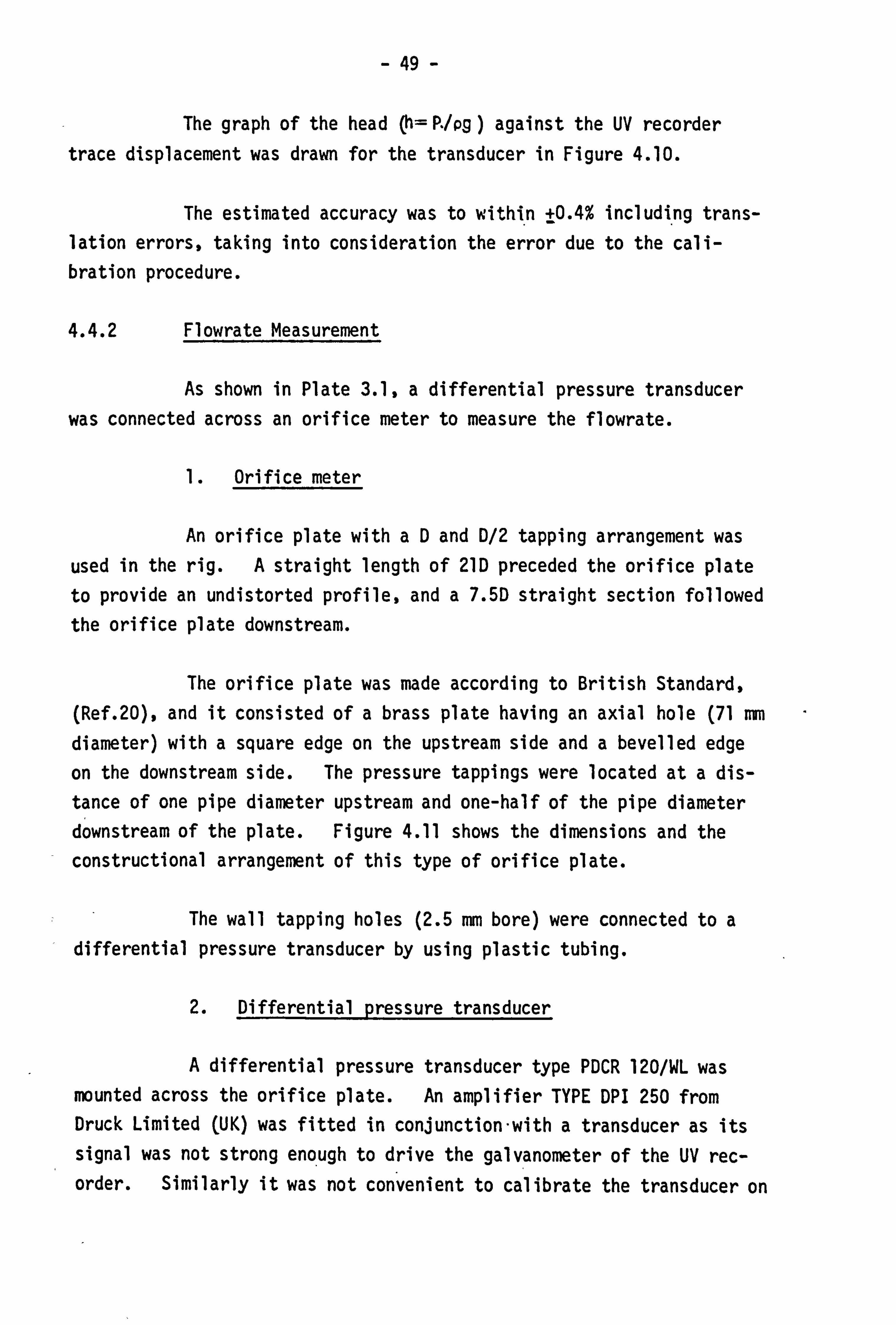
4.4.2 Flowrate Measurement

As shown in Plate 3.1, a differential pressure transducer

was connected across an orifice meter to measure the flowrate.

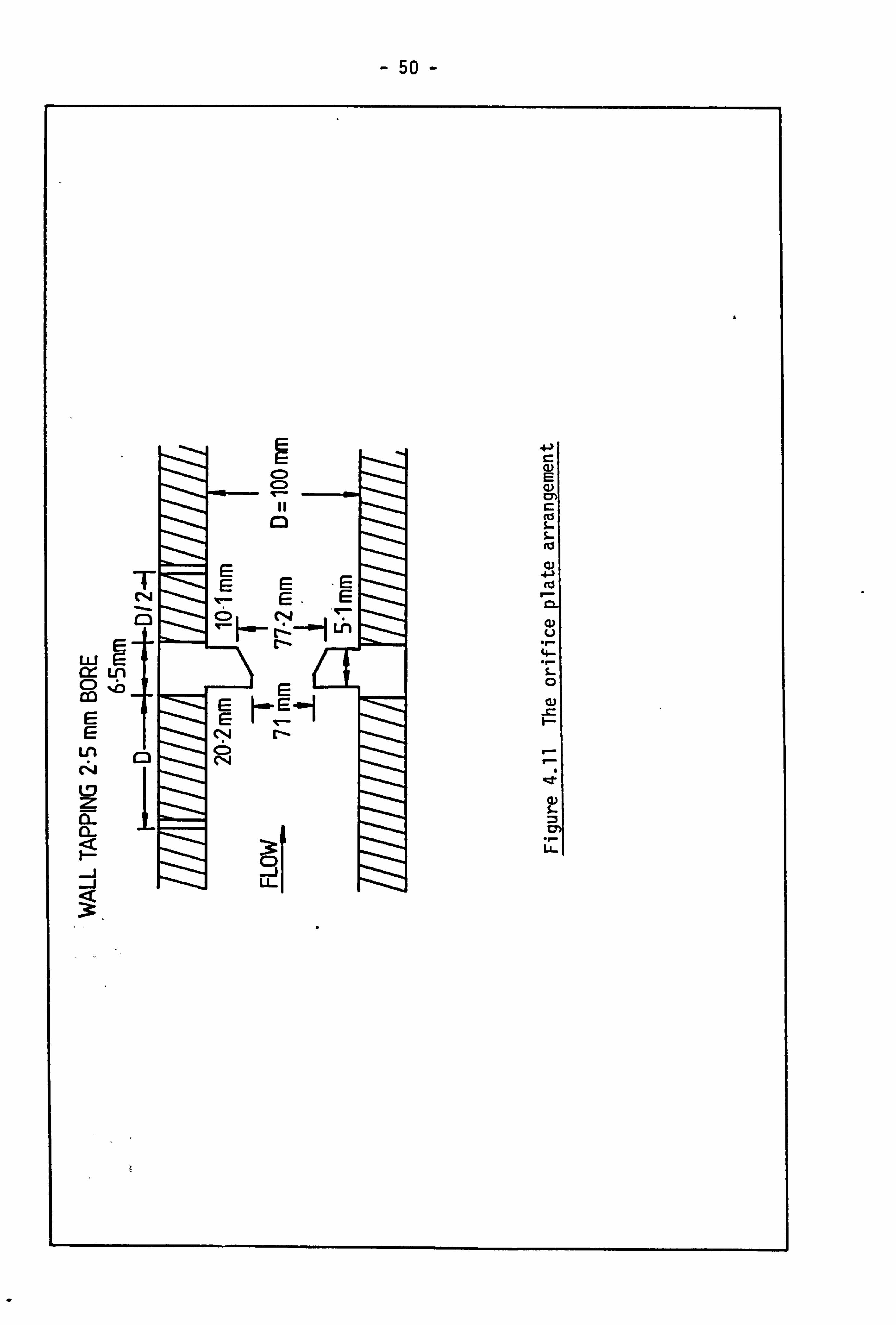
1. Orifice meter

An orifice plate with aD and D/2 tapping arrangement was used in the rig. A straight length of 21D preceded the orifice plate to provide an undistorted profile, and a 7.5D straight section followed the orifice plate downstream.

The orifice plate was made according to British Standard, (Ref. 20), and it consisted of a brass plate having an axial hole (71 mm diameter) with a square edge on the upstream side and a bevelled edge on the downstream side. The pressure tappings were located at a distance of one pipe diameter upstream and one-half of the pipe diameter downstream of the plate. Figure 4.11 shows the dimensions and the constructional arrangement of this type of orifice plate.

The wall tapping holes (2.5 mm bore) were connected to a differential pressure transducer by using plastic tubing.

2. Differential pressure transducer

A differential pressure transducer type PDCR 120/WL was mounted across the orifice plate. An amplifier TYPE DPI 250 from Druck Limited (UK) was fitted in conjunction-with a transducer as its

signal was not strong enough to drive the galvanometer of the UV recorder. Similarly it was not convenient to calibrate the transducer on

- 50 -

E 4-)

E-=

co

E EE

(D 4J

c, j EE CL

Ln E- L) E r. Lu E

4-

IX C) Ln

%b E E

E E E In 0 CN 64 Zz d LV

-j U-

- 51 -

site, therefore a special tester built by the BHRA Instrumentation Dep-

artment was'used. Figure 4.12 shows the pressure circuit. The electrical circuit, also shown on this figure, consisted of the transducer,

an amplifier unit and UV recorder.

The calibration procedure was as follows. Initially the UV recorder trace position was noted for the zero signal corresponding to atmospheric pressure. The damping valve was opened to create a pressure difference in the manometer then closed. The pressure difference in the manometer is equal to the pressure difference across the transducer. By using the adjustment valve, a range of differences

can be obtained.

The resulting trace displacement was measured relative to the zero signal position and the corresponding pressure difference in the manometer was found. The volume flowrate (Q) in the pipe was then

related to the manometer pressure difference readings as follows:

0.01252 KA7p- M3 A (4.4)

where K is the product of several correction factors given in the British Standard, h is the pressure difference in m of water and P is the

water density (kg/CM3). The calibration curve of the flowrate (Q)

against the UV recorder trace displacement is shown in Figure 4.13.

A high natural frequency allows measuring any variation in flowrate. From the natural frequency of the differential transducer it can be estimated that the response time is about Ix 10-5 sec. Also the response of the water in the plastic tubing was 1x 10-5 sec. according to Brown and Nelson's formula, (Ref. 26).

pt = erfc

i To (4.5)

iI -h - -ro

I

where Pt = the desired transducer pressure Pi = the initial pressure

T= dimensionless time = tv/r 2

- 52 -

-ro = dimensionless delay time =T /r 2

v= kinematic fluid viscosity r= pressure tubing radius T= tubing length/acoustic velocity = L/a

erfc = the complimentary error function.

The accuracy of the measurements were subjected to many sources of *systematic and random errors which are explained below.

The major source of error was the manometer reading used in

calibration of the transducer. The estimated accuracy was within 0.5%. The combined errors of the transducer and the amplifier output was ±0.05%.

The total error in flowrate measurements by using the orifice plate in conjunction with a differential pressure transducer was +0.55%.

- 53 -

Ll

-0

ui

ui >

t Li L. U >

i L L

co _ j

4-) C (U L

42 i 4-

15 4- 0

4J

L) S-

C 0

4-)

cli

S-

LLJ

- 54 -

F)

C: )

C>

C)

Co

CD r-

CZ) %0

C> Ln

CD .. t

C> rn

9

CD 92

C)

S.

-v

r-

4- c Q

(A rm r-

14. ui c L. ) <

F5 ;I

c) LJ

C,. I-

.r u

Z(sl I)ZD 31V8 MOIJ

- 55 -

4.4.3 Speed Measurement

A variable reluctance tachometer is often used to measure the speed of a shaft, (Ref. 21). Tachometers, using a toothed rotor made of ferromagnetic material and a transduction coil wound around a permanent magnet are the most common form of pulse output speed transducers Figure 4.14. The magnetic field surrounding the coil is distorted by the passing of a tooth carrying a pulse of output voltage in the coil. The root mean square (rms) value of the output voltage increases with a reduction in the clearance between rotor and pickup with an increase in tooth size and with an increase in rotor speed. The frequency of the output pulses is dependent on the number of teeth and the rotor speed and they are counted to determine the rms value. Usually about 60 teeth are used and clearance is about 0.3 m, (Plate 4.2).

The output voltage is fairly sinusoidal and the peak-to- peak value proportional to the shaft speed ( 11 rev/min).

It is easy to calibrate the tachometer on site. The output of the pickup is connected to the UV recorder. Different speeds are recorded by varying the gate opening and hence the speed of the turbine.

The calibration curve of the speed (N) against the UV recorder trace displacement is shown in Figure 4.15.

- 56 -

LL.

0) c M

-57

Alk-

mm ý

PLATE 4-2 THE TACHOMETER

I 4

'0

I

- 58 -

L.

0

cc r- %0 Ln rn C*4

(OoLx -w-dj) 033dS

ýq!

"

- 1ý e

E ca 4: > -w

14- c

C::

F-

c

4-ý Ln F5

cc S.

>

Lf 9- ml

PR 5 cr . r.

Li-

C: ) C*4

ci q-

ON

- 59 -

4.4.4 Gate Opening Measurement

One of the most common transducers in control systems ap-

plications is the potentiometer which converts mechanical position into

an electrical voltage, (Ref. 21). Figure 4.16 shows a schematic and block diagram of the relation between the input output voltage and the

mechanical position of the shaft.

REFERENCE VOLTAGE R, SOURCE R 21 Vi

SCHEMATIC

SHAFT POSITION INPUT

-0 Vo

VOLTAGE OUTPUT

BLOCK DIAGRAM

v POSITION

POT VOLTAGE

vo i INPUT I

OUTPUT

Figure 4.16 Schematic and Block Diagram of the Potentiometer

The wicket gate opening was recorded as follows.

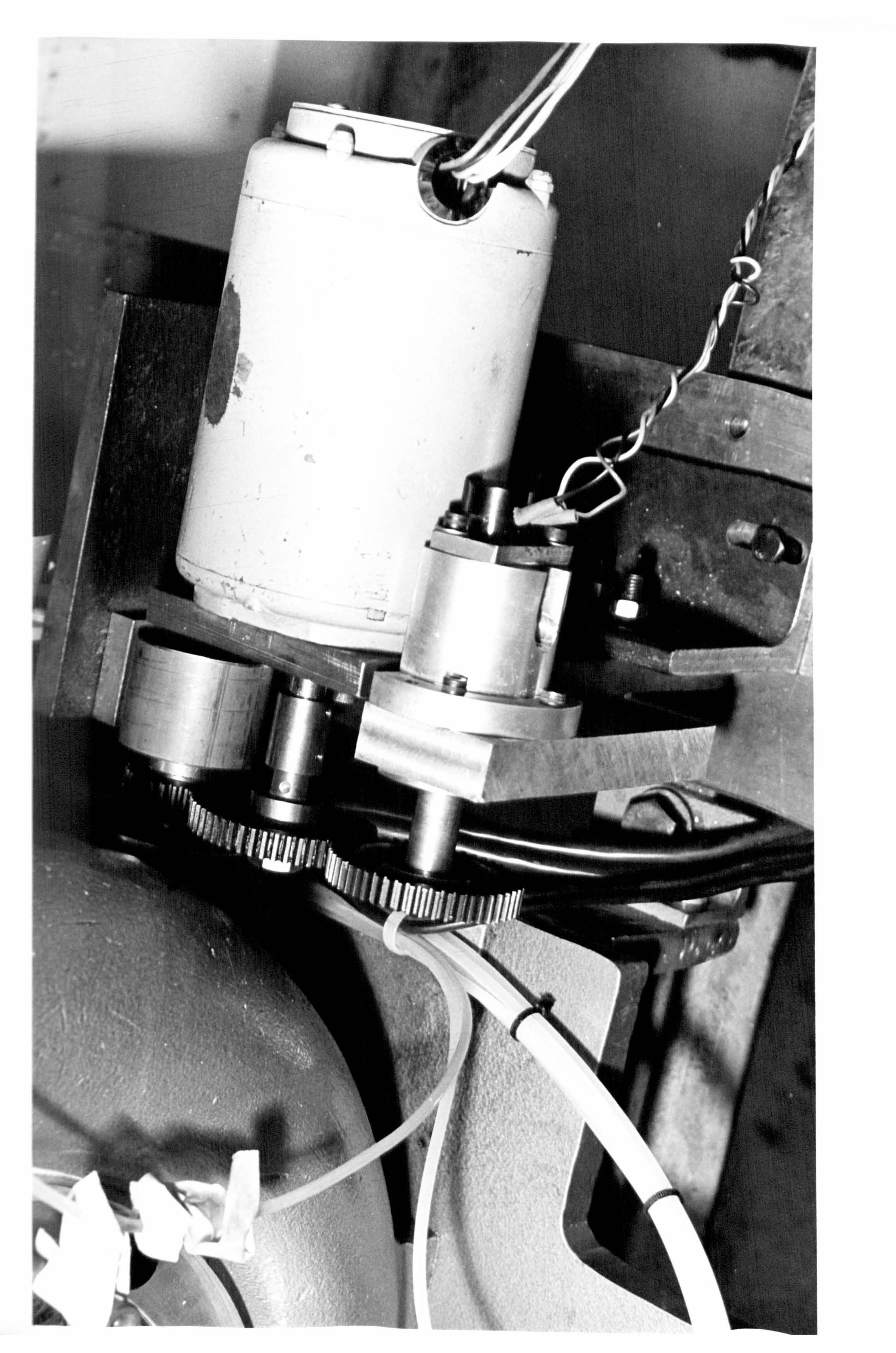
Two gears were used with a1 to 4 ratio, the small one con-

nected to the stepping motor shaft and the large one connected to a potentiometer which converted the mechanical position into an electrical voltage, Plate 4.3. The relation between the mechanical position and the output voltage (VO) is linear because both of them depend on the

potentiometer position (i. e. R2/Rl) which is varied.

The calibration of the gate opening is as follows.

When the gate is fully opened a particular signal is obtained from the potentiometer and recorded on the UV recorder. This signal

ry CD CD . Y-

Q- LLJ

V) cr LU

LU 7- CD

.Z LU

Z:

CD h- CD Z

(D

a- LU

ui T-

- 61 -

B

CD Pli

LLJ

C) LLI cu C74 4-4

to

CL)

Q LLJ 4- co Sý o

Lý

C) Ln C) Ln In e4

M DNIN3dO 31VE)

LL.

2 c**4

- 62 -

represents 100% gate opening. The 0% gate opening is obtained by

closi. ng the gate manually a nd the output signal recorded also. The

calibration curve of the gate opening is shown in Figure 4.17.

4.5 EXPERIMENTAL METHOD

A full set of tests were carried out for a range of partial load rejections as well as for full load rejection. Appendix B tabu- lates all the experimental results.

At the beginning of the experimental work on the rig it was essential to calibrate all of the instruments used for data collection. Normally one test run was carried out during a single day. The amplifiers and the UV recorder needed to be switched on one hour before the test. The experimental procedure is detailed in the following items.

1. The supply pump of the system was switched on and the

required conditions of head and flow were obtained by using the gate

valves.

2. The load imposed on the turbine can be fixed by using the plug in points (1-15), i. e. for full load rejection plug in points I and 15 were used.

3. The output of each part of the controller (PID) was checked to ensure that it was zero in each case.

4. Initially the conditions were determined in terms of the following measurements.

(a) The speed of the turbogenerator set by

recording the control console indicator

on the UV recorder. (b) The flowrate by recording the pressure

difference from the amplifier on the UV recorder.

(c) The inlet pressure recorded on the UV

recorder.

- 63 -

(d) The gate openi. ng by using an avometer for the output of the potentiometer and the UV recorder

(e) The load imposed on the turbine by the

generator from the voltmeter and ammeter of the control console.

5. The UV recorder and the stepping motor supply were switched on and at the same time a load rejection was done by manually switching off.

6. The speed of the turbine increased suddenly then the feedback response actuated the stepping motor to close the gate of the turbine till the speed returned to its initial value. The motor ro- tated clockwiseor counter clockwise when the speed was less than the demanded speed.

7. At the end of the test when the fluctuations were stopped (steady state), the stepping motor supply was switched off as well as the UV recorder.

8. Upon attaining the required steady state conditions the above procedure (Items I to 7) was repeated for different load rejection.

Each test was repeated many times till consistent results were achieved. This was necessary because of the sensitivity of the

electronic system and due to the hysteresis in the mechanical parts.

- 64 -

CHAPTER 5

COMPUTATIONAL PROCEDURE

5.1 INTRODUCTION

The computer program consists of a "MAIN" program and several

subroutines and functions. The main program serves primarily as a device for linking the subroutines together in proper sequence and, in

addition, performs certain bookkeeping and test computations at the be-

ginning and end of each time step. The total program is perhaps most easily described by first discussing the subroutines and functions and then showing how they are combined in the MAIN program.

5.2 FUNCTIONS (see flowcharts on pages 75-82)

5.2.1 Function FACT (1, J, K, L, PHIO)

This function Is used to calculate the Lagrangean interpolation

coefficients li(x). Hence

2 (x-x

0 )(x-x, ) ............ (x-xi-1)(x

(X i -x 01 ýV .. (X i-xJ-l X

n X-x . (x) = I, (r)

rmi xj-xr rýi

By substituting x=0

I NO Ogiven - Or

) 1 (0) ý 11 ("

r=l Oi - Or rii rýk oi

-x i+. l )*0*6 (X-xn) x J-XJ+1).. (X i -Xn

(5.1)

(5.2)

- 65 -

. 4.. -ý whco, k and Z are the subscripts of 0 when the function calculates the first and second derivative of Lagra

, ngean interpolation coefficients

I i(x) and P Number of unit speed tabulated Ogiven The unit speed calculated.

5.2.2 Function FLAGI(N, X, I, Xo)

This function is used when all the points in the grid of the turbine characteristics are used to calculate: -

1. z when the general Lagrangean formula Is used. Hence

NT T given - 'rr) (T) 0 11 (TT (5.3)

r=l I-r Ni

whe re X= 0 T given = The gate opening calculated

NT = Number of gate openings from the turbine characteristics.

2. 'Ei(q) when the gate opening at t=O is calculated, i. e.

Tf (q, ý)

Nq q giyen q i(q)

r=l " qj -qr 04

where X0 =q T given a The unit flow calculated from the initial conditions.

Nq = Number of unit flow from the turbine characteristics.

5.2.3 Function FLAG(I, J, PHIO)

(. 5.4).

. This is used to calculate the Lagrangean interpolation co-

efficients of equation (3.44) and is the equivalent of Function FACT (1, J, O, O, PHIO) with K=L=0.

- 66 -

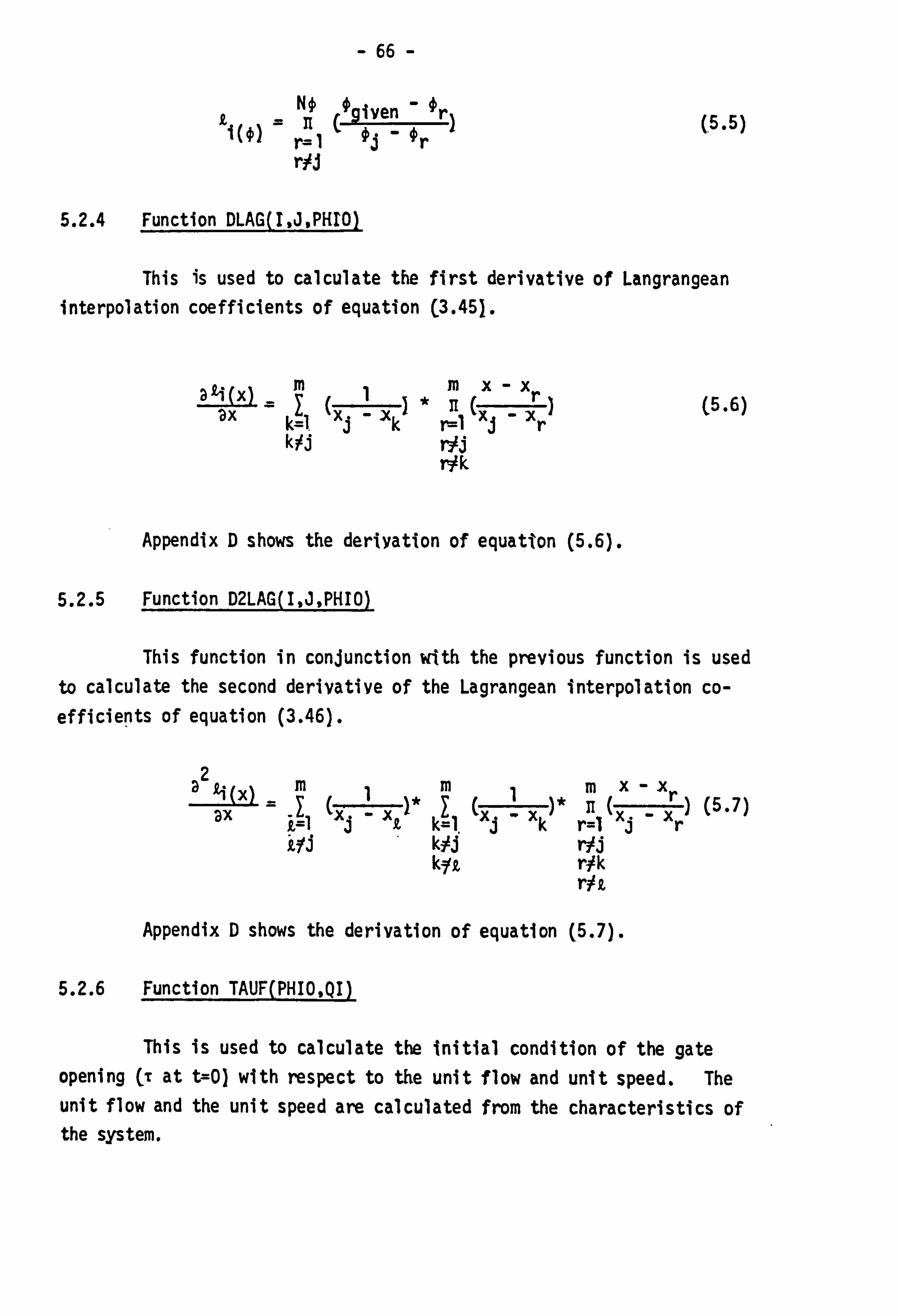
L Ne e iven - n, g. 5) i (e) m =, -, r= 1 ýj - ýr rýi

5.2.4 Function DLAG(I, J, PHrO)

This is used to calculate the first derivative of Langrangean interpolation coefficients of equation (3.451.

3 li (x) -m1mx-x j( -) k 1, (_ r (5.6) i- -Z xkZ, -x )

kil re- 1jr kýj rii

rýk

Appendix D shows the deriyation of equation (5.6).

5.2.5 Function D2LAG(I, J, PRIO)

This function in conjunction with the previous function is used to calculate the second derivative of the Lagrangean interpolation co- efficiepts of equation (3.46).

2mX -X 4 (x) r

ax i ciý) )* n() (5.7)

i=i Z1-xx xk r=l xi r kli kij r1/i

k-I. t rýk rA

Appendix D shows the derivation of equation (5.7).

5.2.6 Function TAUF(PHIO, QI)

This is used to calculate the initial condition of the gate opening (, r at t=O) with respect to the unit flow and unit speed. The unit flow and the unit speed are calculated from the characteristics of the system.

- 67 -

qn q3

q2

91 Y2 93 On Ogiven

The function is worked in two steps.

Irrm

r, 2

1. For a given unit speed (fl where q= f(ý, T), the unit flow can be calculated from equation (3.43).

mm Ogiyen Or qC, i 'or) (5.8)

r-l i rii

The co-ordinates at ý given are:

I, N

where N,, = Number of gate openings.

2. The previous results represent a one dimensional relation between qi and Ti . Then

Nq Nq qq Ir (given - r) T (5.9) initial ý

j=l r=l qj -qri Ni

- 68 -

q

given

5.2.7 Function ZI(7AUI, PHrI, Z, ID)

The previous functions are controlled by this function, where (Z) refers to the two dimensional performance data of the turbine and CID) refers to the functions.

Also the function works in two steps.

1. For 0 given and T given' z i, is calculated from equations

(3.44), (3.45) and (3.46).

z ZV1j4)

ven

,ý For Zi calculated and Ti defined, Z can be calculated.

Z2 - ZI Z= (

T2 - Tl )(Tgiven - TI )+z1 (5.10)

Tinitial T

(: ýgiven

- 69 -

z2

z

zi

5.3 SUBROUTINES (see flowcharts on pages 83-90)

5.3.1 Subroutine DATA(IDATA)

All required data are stored by the subroutine data. It can be divided as follows: -

1. Initial conditions data (Appendix C). 2. The turbine performance data which are stored in a two

dimensional table of values of unit speed vs. unit flow and unit speed vs. unit power for various gate openings (Appendix Q.

5.3.2 Subroutine LINEAR(TAUI, PHII, QI, AOsAl)

The constants a0 and aI of equation (3.23) are calculated as follows. By rewri ti ng equati on (3.231 wi th q and ý known

a0+a, ý (3.23)

Differentiate both sides of the equation with respect to ý.

*= a1 (5.11)

To evaluate Function ZI(TAUI, PHII, Z, ID) for Z Q, the data required are unit flow vs. untt speed for various gate openings and with ID =I which refers to the first derivative of equation (3.44), al my be calculated. Hence

rr Tgiven 2

- 70 -

ao q-y

5.3.3 Subroutine PARABOLIC(TAUI, PHII, C0, CI, C2)

The constants Cos C, and C2 of equation (. 3.14) can be calculated as follows:

I Rewriting equation (3.141

c+C2 0 1ý

Differentiating both sides of the equation twice with respect to ý

dp, C+ 2C (5.13) W12

d2 2 (5.14) C2 dý

To evaluate function ZI(TAUI, PRII, Z, ID) for Z P, the required data are unit flow vs. unit power for various gate openings and ID=0,1,2

which refers to equations (3.441, (3.45) and (3.46). Then

C=0.5 d (5.15) 2 -24 dý

C= dp - 2C (5.16) 1 7aF 2ý

c ": p2 (5.17) 0- Clý - C2ý

5.3.4 Subroutine ITER(N, QP, TAUI, PHII, HN, HP, CP, IC)

The aim of subroutine ITER is first to calculate the gate opening at t=O and secondly to calculate the flowrate (QP), net head (HN) and piezometric head (HP) at the end of each time step as follows:

- 71 -

1. At t=O tile initial conditions of the speed (NJ, flowrate (Q) and net head CHN) are known so unit flow and unit speed can be calculated. The gate opening at t-O may be calculated from Function TAUF in conjunction with Functions FLAG and FLAGI.

2. At t=, &t, the input data are N and T calculated by the Runge-Kutta subroutine and Cp calculated by the subroutine character. To calculate the unit speed at t-=&t, the net head is required but it is

unknown. However by combining equation (3.7) and equation (3.22) and assuming Qpt=o = Qpt+At

HN ý CQp-(S2*. Qp - ')+ Cp)'Sl - HT (5.18)

where SGx AREA A

s1 2= 2CAREA)CAT

and A= water hammer wave velocity (p1s) AREA = cross sectional area of pipe (m 2

Thus, the unit speed is known and the unit flow can be calculated, also the constants AO-A6- Then the flowrate at t=At is

calculated from equation (3.25) and HN, Hp from equations (3.24) and (3.22). However, if IQP -, QPassuml :' 0-0001 then the above procedure should be repeated to refine the solution.

that 3. If t> At, the same procedure of (2) is repeated except

Qpt = Qpt-At

and HN =C(Qp - A3)/A 2) 2

- 72 -

5.3.5 Subroutine RUNGE(PHII, TAUI, HN)

The equations (3.16), (3.33), (3.35), (3.38) and (3.41) are solved simultaneously by the fourth order Runge-Kutta method. The initial conditions of all the variables in the equations are required. N is known,

-r calculated by subroutine ITER and all the governor parameters are set to zero. All the equations are non-dimensionalised by dividing all the

parameters by a reference value.

N ref ý- synchronous speed

Tref = gate opening at t=O

(V p

VISV D' V Alref *ý 1 (because their initial values are zero and hence could not be used).

From Runge-Kutta integration all the parameters are found at t=At.

5.3.6 Subroutine CHARACTERCIC, ýpl

The object of this subroutine is to calculate Cp as well as the pressure and the flowrate in the pipework. The pipework is divi-

ded into 16 reaches. The boundary conditions were derived in Chapter

3. A Newton-Raphson method was used to solve the upstream boundary

condition.

Rewriting equation C3.21)

Q =/ - Xýýs

(3.21) '9.55

assume

From equations (3.21) and (3.6) with Hs = 1.0 and Ca ý- S, we get: -

- 73 - 3 GI + Ry + Eý + Vy +HB=0 (5.20)

where G= (6.2 x SI) 2

R= 12.4 x S, F=- (CN + 115 x SI) V= 2F E=1+RxF+6.219.55

HB= F-F - 114/9.55

Equation (5.20) is solved by using Newton-Raphson method.

Yi 'ý Yi-1 (5.21)

where F'(y)i_l is the differentiation of equation (5.20) with respect to (y).

5.4 THE MAIN PROGRAM

The principal functions performed by the MAIN program are listed below:

The various equations generating subroutines are linked together in proper sequence. The equation-solving iterations are controlled and tested for convergence.

(iii) Incrementing computations are performed. (iv) Input and output are controlled.

5.5 SUMMARY OF THE COMPUTATIONAL PROCEDURE

1. Q, HN and N are known initially so the gate opening (j)

can be found by Lagrangean interpolation (equation (3.44)) at. -r=f(q, ý).

2. The initial conditions of the variables in equations (3.16), (3.31), (3.33), (3.35) and (3.41) are required. N is known, T calculated and all the governor parameters are set to zero.

- 74 -

All the equations are non-dinensionalised by dividing all the

parameters by a reference value.

From Runge-Kutta integration all the parameters are found at t=At.

3. The method of characteristics CRef. 5), is used for cal- culating head and flow throughout the system.

A printout of the computer program is in Appendix E.

- 75 -

Flow chart of the function FACT(I, J, K, L, PHIO). Calculation of the Lagrangean interpolation coefficient.

- 76 -

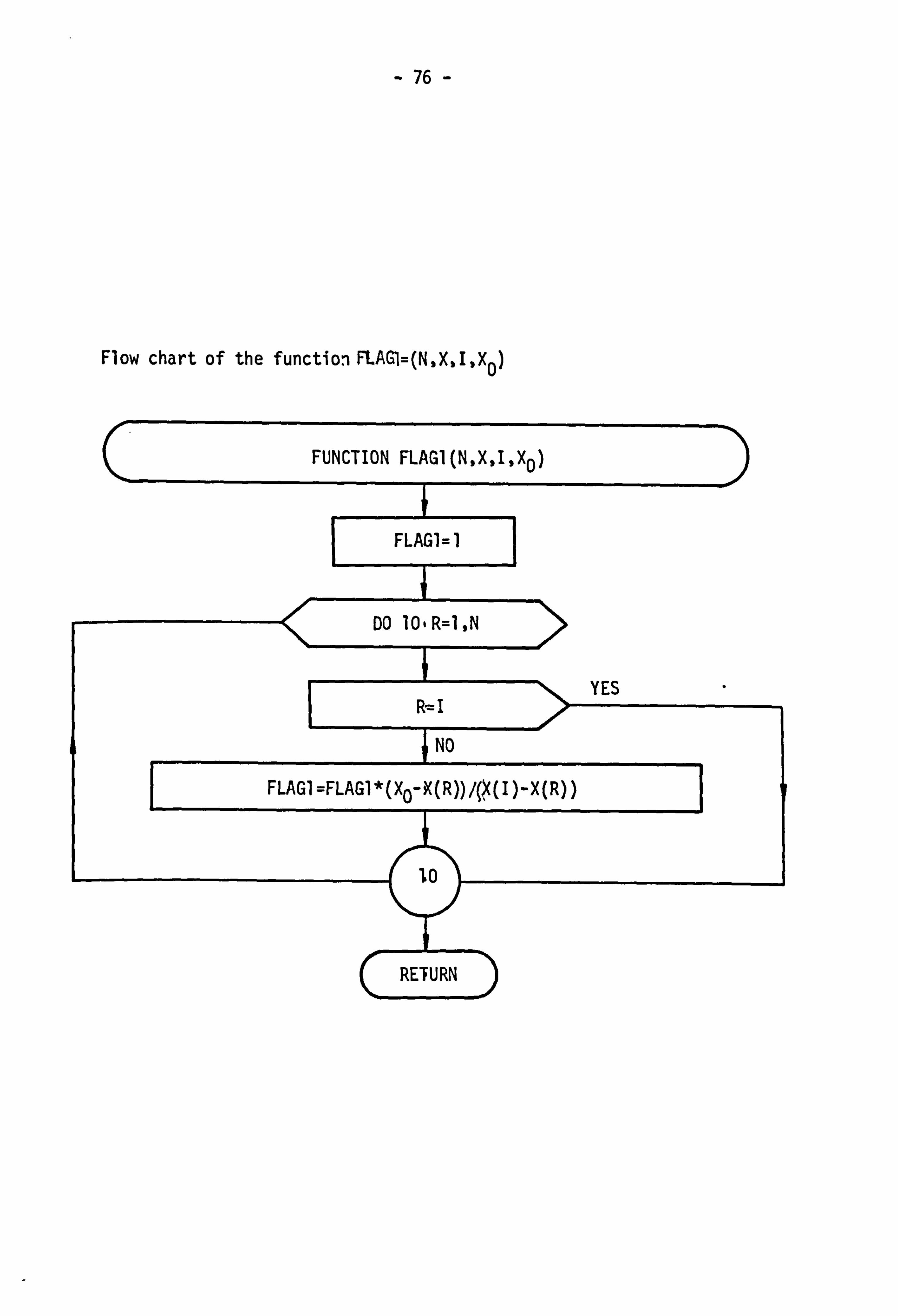
Flow chart of the function FLAGI=(N, X, I, Xo)

- 77 -

Flow chart of the function FLAG(I, J, PHIO) to calculate kI (X)

FUNCTION FLAG(I, J, PHIO)

FLAG=FACT(I, J, O, O, PHIO)

RETVRN

- 78 -

Flow chart of the function DLAG(I, J, PHIO) to calculate ax

- 79 2

.I Flow Chart of the function D2LAG(I, J, PHIO) to calculate - -2-- ý a, X

- 80 -

Flow chart of the function TAUF(PHII, QI). to calculate the initial condition of the gate opening (T).

FUNCTION TAUF(PHII, QI)

DO 50 I=I, NTAU

>=O. 0

DO 50 J=i, NPHI(I)

Y(I)=Y(I)+Q(I, J)*IFLAG(I, J, PHII)

TAUP=O. 0

DO 100 I=I, NTAU

TAUF=TAUF+TAU(I)*FLAGI(NTAU, Y, I, QI)

REURN

- 81 -

Flow Chart of the function ZI(TAUI, PHII, Z, ID)

FUNCTION ZI(TAUI, PHII, Z, ID)

DO 10 I=J, NTAU

[-TAUI<TAU(I) YES...

NO

-0 110

I NI=NTAU-1

1 1-01 30

-0 NI=I-1 I

I

-, f

Nl<l YES

N L=l

30

Ile, DO 50 I=NI, Nl+l %I'- ý-

>

t F-Y

(I)=O. O

-T- ooe- DO 50 J=I, NPHI(I)

ID=O

F=FLAG(I., J, PHII)

r1i)

- 82 -

NO I D--l

YES

ID=2

Y(I)=Y(I)+F*Z(I, J)

F=DLAG(I, tJ, PHII)

F=D2LAG(I, J, PHII)

ZI=Y(NI)+(Y(NI+1)-Y(NI))/(TAU(NI+1)-TAU(NI))*(TAUI-TAU(NI))

RETURN

- 83 - Flow chart of the subroutine DATA(IDATA)

SUBROUTINE DATA(IDATA)

READ, NTAU

READ, (TAU(I), I= I, NTAU)

DO 10 Ir-1, NTAU

oof READ, NPHI, (I)

READ, (PHI(I, J), Q(I, J), J=I, NPHI(I

READ, -NTAU2

NTAU2, NE. NTAU >-M-f STOP

, (TAU(I), I=1, NTAU)

DO 2Q I, =I, NTAU

READ NPHI(I)

L---fREAD(PHI(I, J), P(I, J), J=1, NPH(I))

READ, DR, D, G, A, HT, NR, QA, HA, F, DT READ, II, PG, ETAG, TI, KP, TA, TD, KD READ, NTIM, c-, QIN, PHIIN READ, K, KM, L, R, KI, KE, SEGHA READ, C, HS, NPA, DX

Cal cul ate So ss, S 2' 's7, R, , R21 R 31 rE-0, EIR, AREX, MC, NC

RETURN

- 84 -

Flow chart of the subroutine LINEAR(TAUI, PHII, QI, A0, Al) to calculate a0ga

,V

SUBROUTINE LINEARCTAUI, PHII, QI, A0, Al )

Al=ZI(TAUI, PHII, Q. 1)

AO=QI-AI*PHII

RETURN

- 85 -

Flow chart of the subroutine PARABOLIC(TAUI, PHII, COqCl9C2) to calculate C09C, %C 2'

SUBROUTINE PARABOLIC(TAUI, PHII, CO, Cj IC2)

C2=0.5xZI(TAUI, PHII, P, 2)

Cl=ZI(TAUI, PHII, P, 1)-2*C2, PHII

CO=ZI(TAUI, PHII, P, Q)-PHII*(Cl+C2*-PHII)

RETURN

- 86 - Flow chart of the subroutine ITER(N, Qp, TAUI, PHII, HN, HP, IC, CP, YN) to calculate Qp, Hp, HN-

SUBROUTINE ITER(N, Q p

TAUI, PHII, HN, HP, IC, CP, YN)

CALL CHARACTER(IC, CP)

! NO Ll IC=l

94 ICv-2 Nio MI

To calculate the constant (Cp)

N=NR, Q p =QA

QP=QA HN=(Qp*(S2-kQp-*I)+Cp)/Sl-HT

IT;: O

10

IT=IT+l

PHII=S3*N/YR

Eq, Icpl -NSYES

QI =S4ýqp/ YFN-

I

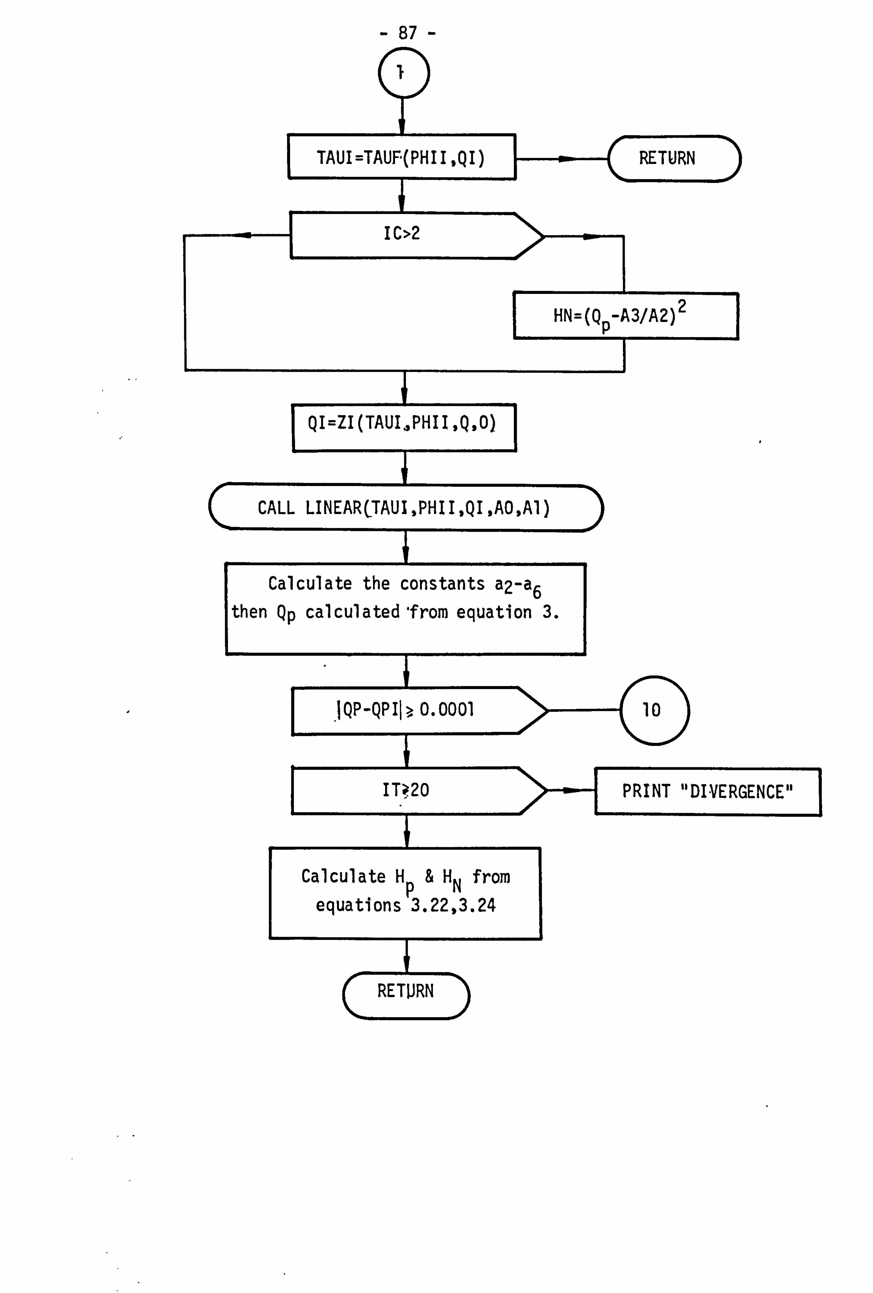
- 87 - I

TAUI=TAUF(PHII, QI) RETURN

I C>2

I HN=(QP-A3/A2) 21

QI=ZI(TAUI., PHII, Q, O)

CALL LINEARCTAUI, PHII, QI, A0, Al)

Calculate the constants a2-a6 then Qp calculatedfrom equation 3.

I IQP-QPII>, 0.0001 >--j 10

ITý20 PRINT "DIVERGENCE"

Calculate HP &HN from

equations 3.22,3.24

RETORN

- 88 -

Flow chart of the subroutine RUNGE (PHI I, TAUI, HN)

SUBROUTINE RUNGE(PHII, TAUI, HN)

CALL PARABOLIC(TAUI, PHII, C09C, 'C2)

Cal cul ate, aPa 8' a9

Equations 3.16,3.33,3.35,3.38 3.41, solved simultaneously to

calculate N, VI, VP, VD, VA, T at the end oT time step'

RETURN

- 89 - Flow chart of the subroutine CHARACTER( I C, CP)

SUBROUTINE CHARACTER(IC, CP)

DO 100 I=1, NPA+l

Q(I)=QA

H(I)=HA-(I-I)*FR

100

RETURN

IC>2

DO 150 1=1, NPA+l

Q(I)=QPA(I)

H(I)=6A(I)

150

DO 201 -I=2, NPA

Calculate QP and HP at the i ntemedi ate

points equation s. 3.11,3.

201

1

- 90

ri

Cp*. calcul. ated from equation 3.3

AI oop for Newton- Raphson iteration

IT=O

19

IT=IT+l

DELYN=FI/F2 where Fl is equation 5.21 171 and F2 its derivative

NO ýDELYPO. 1

-N, ýYE S

DELYN-SING(Q. 1, DELYN)

YN i =YNi,, -DELYN

IYNi-YN- i _., I>o. oooi 'ý>ý 19

IT>, 20 -1

NO PRINT "DI-VERGENCE"

Calculate Hp and Qp(l) from equations

5.21,3.6

RETURN

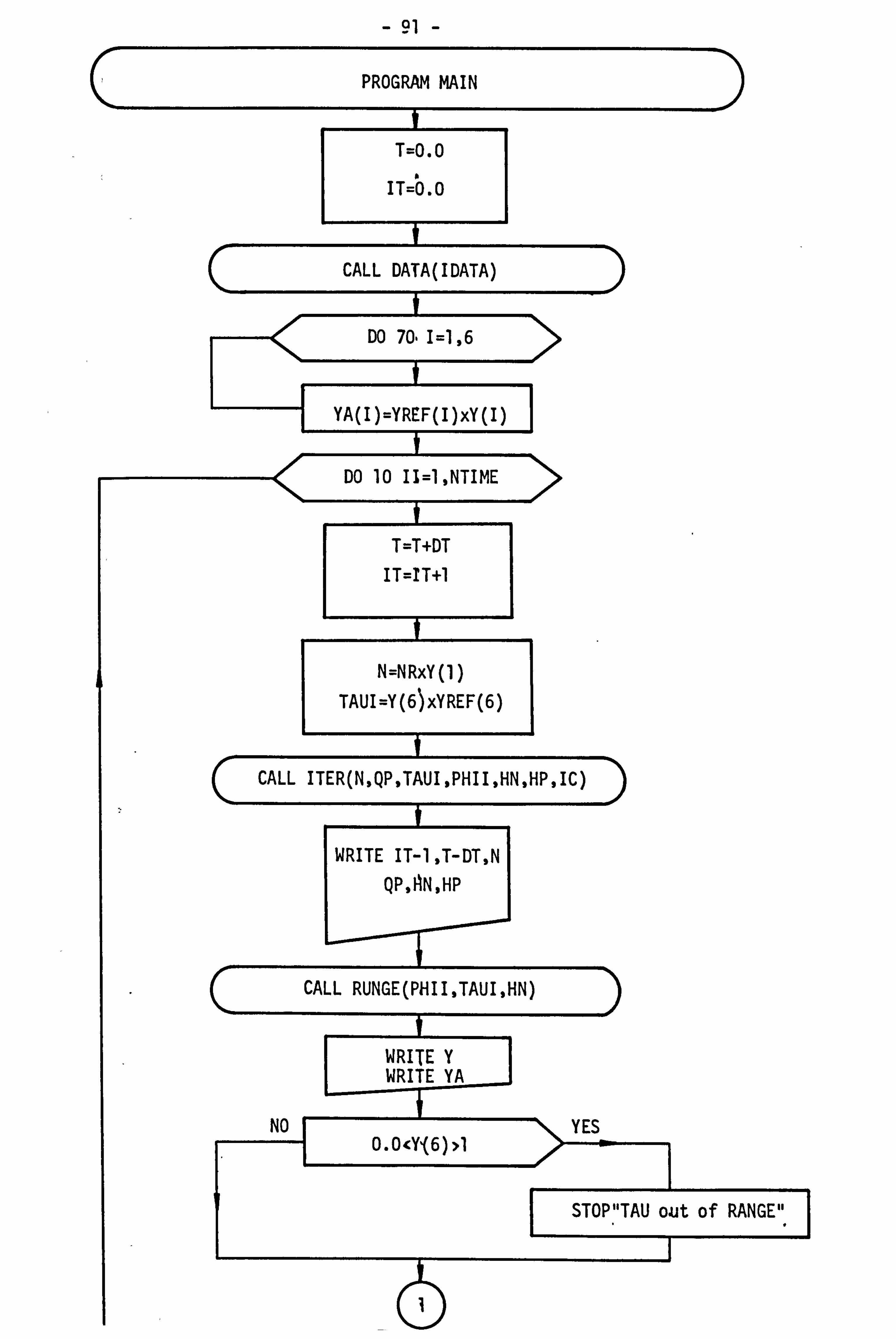
- 91 -

PROGRAM MAIN

T=O. 0

IT=b. o

CALL DATA(IDATA)

DO 70- 1 =1 6

YA(I)=YREF(I)xY(I)

DO 10 Il=l, NTIME

T=T+DT IT=IT+l

N=N RxY (1 ) TAUI=Y(6)xYREF(6)

CALL ITER(N, QP, TAUI, PHII, HN, HP, IC)

WRITE IT-1, T-DT, N QP, AN, HP

CALL RUNGE(PHII, TAUI, HN)

0 Yý

WRIT ,EY WRITE YA

NO -r-- 0.00ý6)>l

STOPTAU out of RANGE"

I

- 93 -

CHAPTER 6

COMPUTATIONAL AND EXPERIMENTAL RESULTS

6.1 INTRODUCTION

The comparisons between the computational and experimental results were made to prove the validity of the equations and assumptions on which the program is based. It was considered particularly im-

portant to verify the Lagrangean interpolation technique and the design

of the proportional, integral and derivative governor. In each case instrumentation was installed for simultaneous and continuous recording of pressure, flowrate, turbine speed and gate position. Also the computed results were printed after every 10 time intervals. The various comparisons are discussed in the following sections.

6.2 FULL LOAD REJECTION

Certainly the most drastic disturbance from the point of view of economic design considerations is the full load rejection. The

governor must close the gate fast enough to limit machine overspeed and yet slowly enough to limit pipework overpressures.

Load was rejected at time t=O. As a result of the load rejection the speed increased and the wicket gates were closed under governor control. Referring to equation (3.16) the incremental values of the speed are positive which mans that the speed will rise, subsequently the speed reduced to speed-no-load condition; as the gate opening decreased towards the speed-no-load value, the total efficiency of the turbine approached zero. On a plot of discharge versus net head the line of zero efficiency represents the locus of steady-state speed- no load conditions. At smaller gate values it is not possible to main- tain synchronous speed without the introduction of an external power source beyond that supplied by the fluid system. Therefore, the corresponding values of total efficiency must become negative, i. e. the incremental values of the speed become negative and the speed will reduce.

- 94 -

InAhe experimental work the frictional resistance and the other losses

alter the speed to reduce it to speed-no-load conditions.

Computed and measured results are plotted in Figures 6.1 to 6.4. As can be seen, the experimental maximum speed is 1% greater than the computed maximum speed Figure 6.1; however, the experimental results show a faster speed reduction than that shown by the computed results. It should be noted that this deviation starts when the wicket gate opening is small. This difference may be due to lack of data for the turbine characteristics at small wicket gate openings. The computed and measured flowrate Figure 6.2, agree closely until t=l. l seconds at which time a rapid divergence( is shown in the experimental results. This difference may be due to error in the differential pressure transducer at very low pressure difference.

Several aspects of the gate time curve shown in Figure 6.3

should be noted. Very soon after rejection of the load, the gate ac- celerated to an almost constant velocity which was maintained until about t=l. l seconds at which time the rate of closure was rapidly reduced. ' As can be seen in the Figure there is a good measure of agreement; however, the experimental results show a faster closure than the

computed results. This difference may be due to the error in the es- timation of the friction losses in the connecting gears and the round-

off error.

The pressure rise curve due to the load rejection is shown in Figure 6.4. The agreement indicated in Figure 6.4 is excellent. The

experimental pressure shows some oscillation occurring at approximately 15 per cent gate opening, at which point the rate of closure is rapidly reduced. The pressure decreases after t=l. l seconds, when the gate variation is very small. According to Ref. 3 and Ref. 7 fluctuation in the pressure/time curves is greater in amplitude and takes a longer time. In our case the fluctuation is smaller and for a short period. A small error in the mathematical representation of the governor could lead to an error in the gate closureltime curve which in turn could lead to a longer error in pressure prediction especially at low gate openings.

- 95 -

The speed and pressure time curves, Figures 6.1 and 6.4-., show that the percentage rises are 26% for the turbine speed and 22% of its

net head.

Krueger, (Ref. 27), in his technical publication "Selecting Hydraulic Reaction Turbines" stated that the speed rise should not ex- ceed 60 per cent and the permissible pressure range is 25% of the design

pressure,., These results are therefore within these limits.

6.3 PARTIAL LOAD REDUCTION

Figures 6.5 to 6.20 show the transient response following different cases of partial load reduction. It is clear from those figures

that there is a good agreement between the computed and the experimental

results.

In the previous case (full load rejection) the reduction of the

speed depended on the negative value of the efficiency because the final

generator power was zero, but in partial load reduction cases the rise and reduction depend on the difference between the turbine power and the final generator power after partial rejection. In most cases it is

noted that the gate openings reduced and then swung until the speed

reached the steady state speed (synchronous speed). Figures 6.16 and 6.20 show that the swinging happens in the computational results and not in the experimental results. This difference may be due to the es- timation of the actuator equation (stepping motor). It appears that the stability of the governor is greater than the estimated near the

steady state conditions.

The speed time curves for all cases are shown in Figures (6.5), (6.9), (6.13) and (6.17). The experimental and the computed results agree closely except for the 31% load reduction. The experimental results show a faster speed reduction than that shown by computational results. This difference may be due to an error in recording and plotting.

- 96 -

The pressure rise curves show mum peak is reduced at 80% load and di to the difference in the gate motion. immediately after the gate reached the

rapidly to its steady state condition, jection, Figures 6.15 and 6.19.

that the fluctuation at the maxi- sappears in the other cases due

The pressure decreased very fast

steady state position returning especially at the lower load re-

Finally Figures 6.20 to 6.24 show a typical comparison between

all the load rejection tests. The closing time of the wicket gate is

proportional to the load percentage reduction.

- 97 -

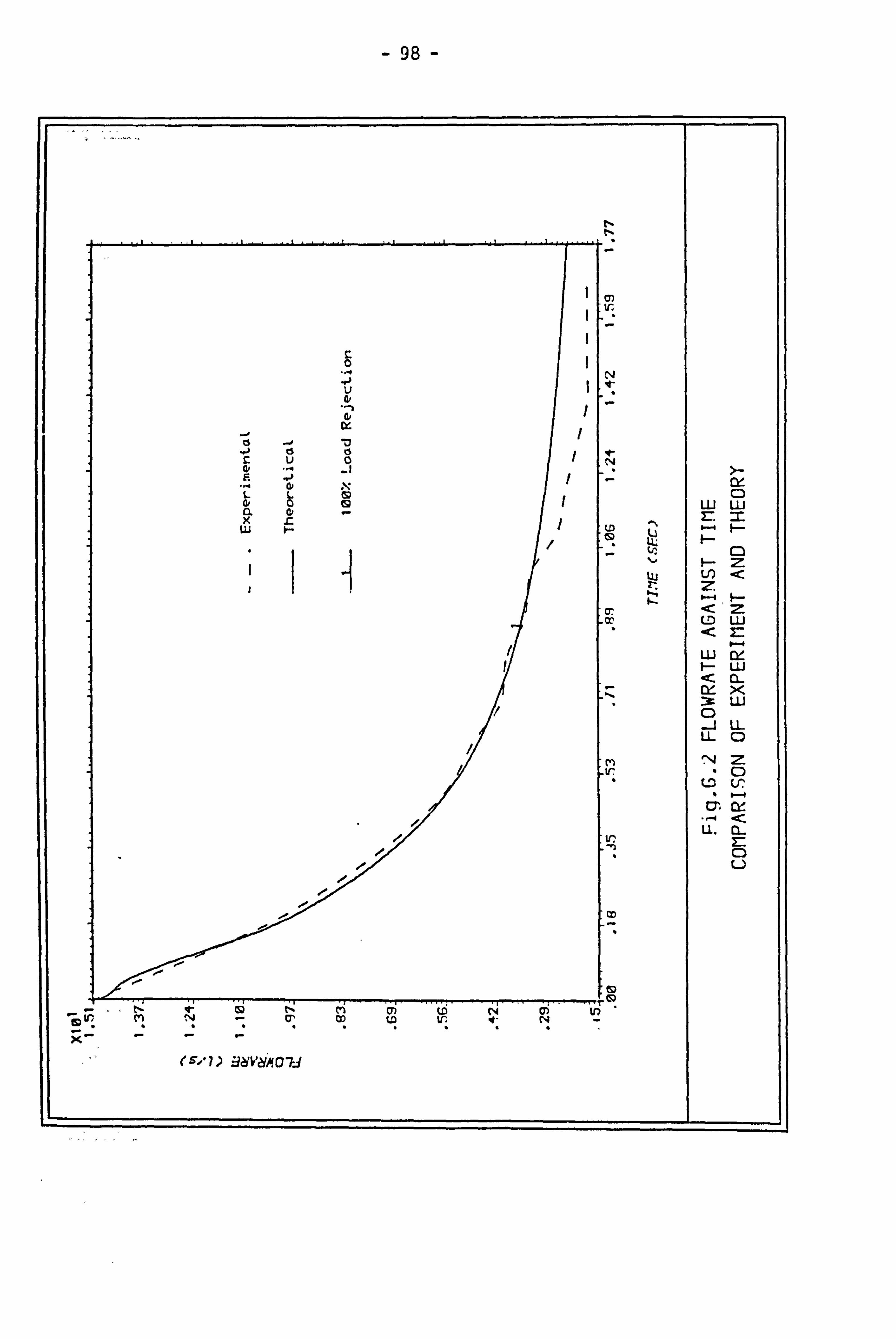
- 98 -

- 99 -

- loo -

- 101 -

- 102 -

I - lU. ) -

- 104 -

ir

u a,

u LU w

1: 7 0 ui

L L. a, c

N, G

(a. x

L;

OD U Lo C2

Z. z

b. ý <

L < U) < z

Lij a, LD

Z

z LLJ LLJ CL

CL X o LU

LU LL 0

0 z

V'. cr, 0 U,

tn w . -cc cm Cl-

tr LL 0

u

tn cp V) ............ ir

cp Ln

Cl) (D In

c Z) VKIIVgciO 01 V-9

- 105 -

- 106 -

- 107 -

- 108 -

Lli

LO z Cl

< <

cl

j -0

cs (7) 1-- LO

z z LIJ =

C. u 0 *--q z

o"

w LLJ Lli L a,

L 0 CI-

0 CL >e a

X. Lli U; f. - LLJ

U- < 0 tD

z N 0

cn - Lr

u CL

Ir LL 0

U

02 co to U7 M

4, :. o') SKIN. 9dC 91 VD

- 109 -

- 110 -

N

0 w w

c 0

u

(Y ts

c ts u

rs 0

U w

Z* a? .., -1 E j

ap LU w L 4p L 0 N LU

>e, --3: LLI 0 --I LL LL C

It- z 0 V.,

<

LL. IL

ir

u

m

Ir LO w (T., ^4 m V)

: 31 V(VA 0 Id

- ill -

a 0 M

10,

N cr in m ED

W)

N 4.

LU 0 z LU

W z z < 1-4 < U z < LL)

1ý r: LIJ 0-4 Lr w

1-4 LU

CY a-

X

ui

ui U-

0

Ln z 0 Ir Lr LO

m < -, -4 a-

LL 3-- 0 u

Co

ý- 112 -

- 113 -

- 114 -

LD N

ts -d 0 LLI

0 LLJ

cu 0 Z7 =- F-

i. N

Lij F- tu

< z LD uj

LU w uj

< IL w A

X LU ir - 0

-1 LL U- 0

C) Lr

LO

co

CL

0

-0 -

u

-1

1ý IS! cn cri cn (P

e ITI, 1 31 VcVA Old

- 115 -

- 116 -

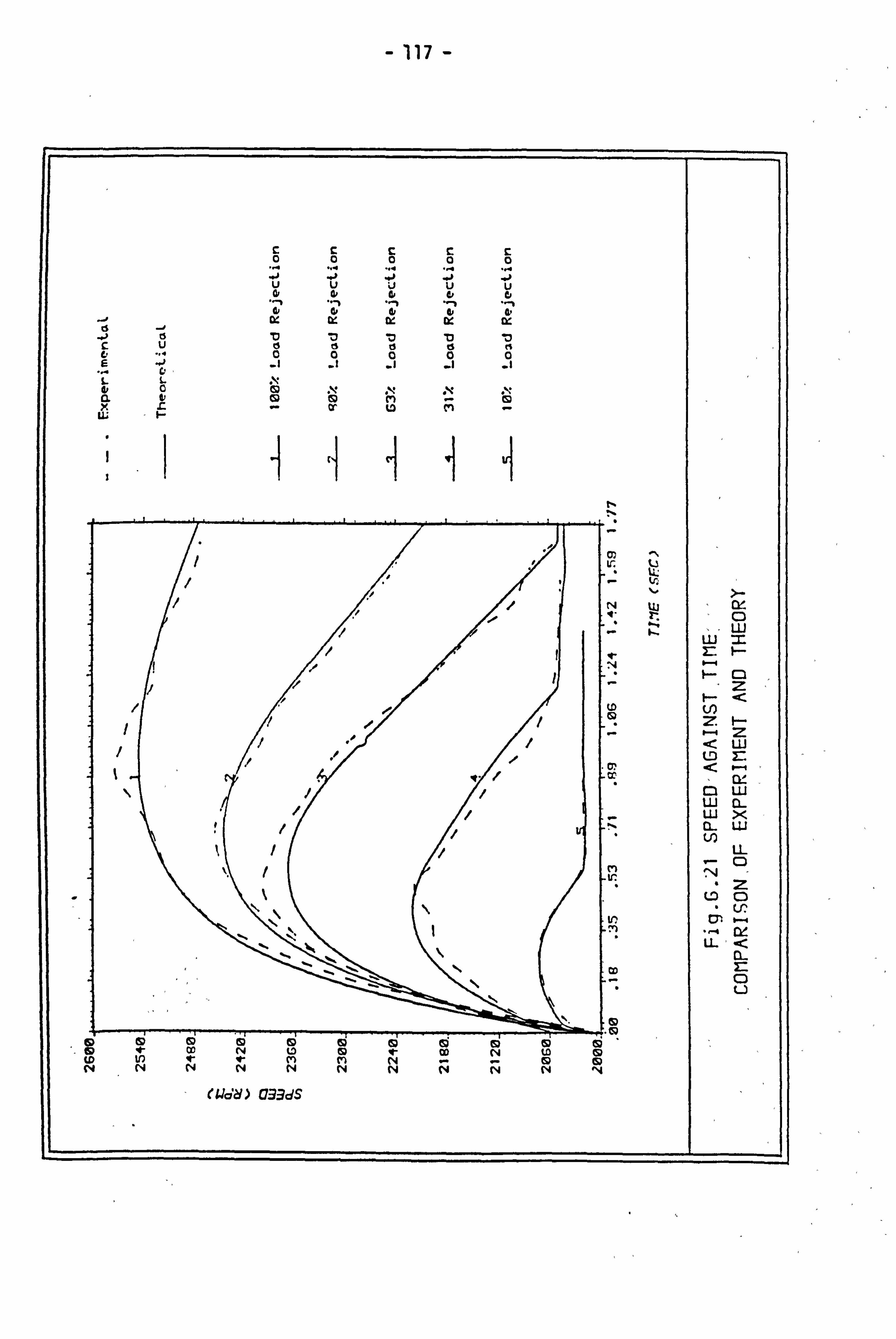
- 117 -

u u u u

-0 ts 1)

N, N N CL x C

CP or

cn Lo cn

CS) LL;

Lr

0

LU r_

Cl z

LLJ

ol LD

Cl LLI LL) LU

CL x

(I- LLI Ln

LL 0-

C-0 0

Cý Uý

LL

OL

X:

0

u

4 co N OD to CD V) NN N

N N

CS)

- 118 -

I

c c c c 0 0 0 0 .j u -1 v -0 u -0 u -0 u 4, 41 41 4p

a: De w D: CK ts .1

ti 15

L 0 ei)

Q. x all co ei) ac (n

Lr tj ,

1 11 N tu LU C)

Z: U-i 6-4

M

(f) z

z <

<

LO z

< Lij

LU

cr < LLJ

_nl: >e C LU

LL LL 0

N z

LO 0 V.,

Lr

U CL . 0

u

eoll) 91 V18A c Id

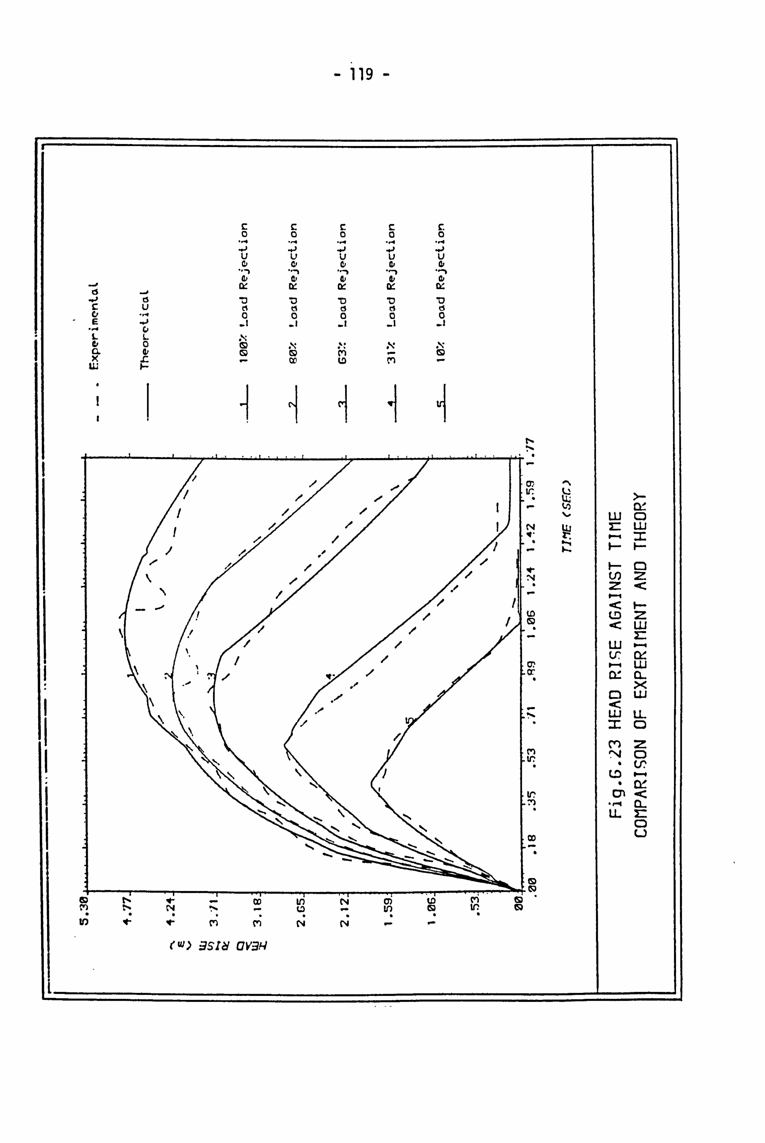
- 119 -

ýj u j

u j

u j u

d, a#

-P C: ts u -j 0 -j 0 "D cs

m (5 c?

E 0 a 0 0

L 0 (S) N

CL x

4ý 0 Q co

(n LD fn

CS) ui

Lij 0 LU

Lo

. 01 z <

LO <

z

LU Lr w

LU q* w CL

X I

Cl ui

;z ui U- C

m z N. 0

Lo

tr 4

m < -4 CL U.

u

I

; CS)

tZ cn ea to ýf- le MM N N - -

CW> : 331cy cvgq

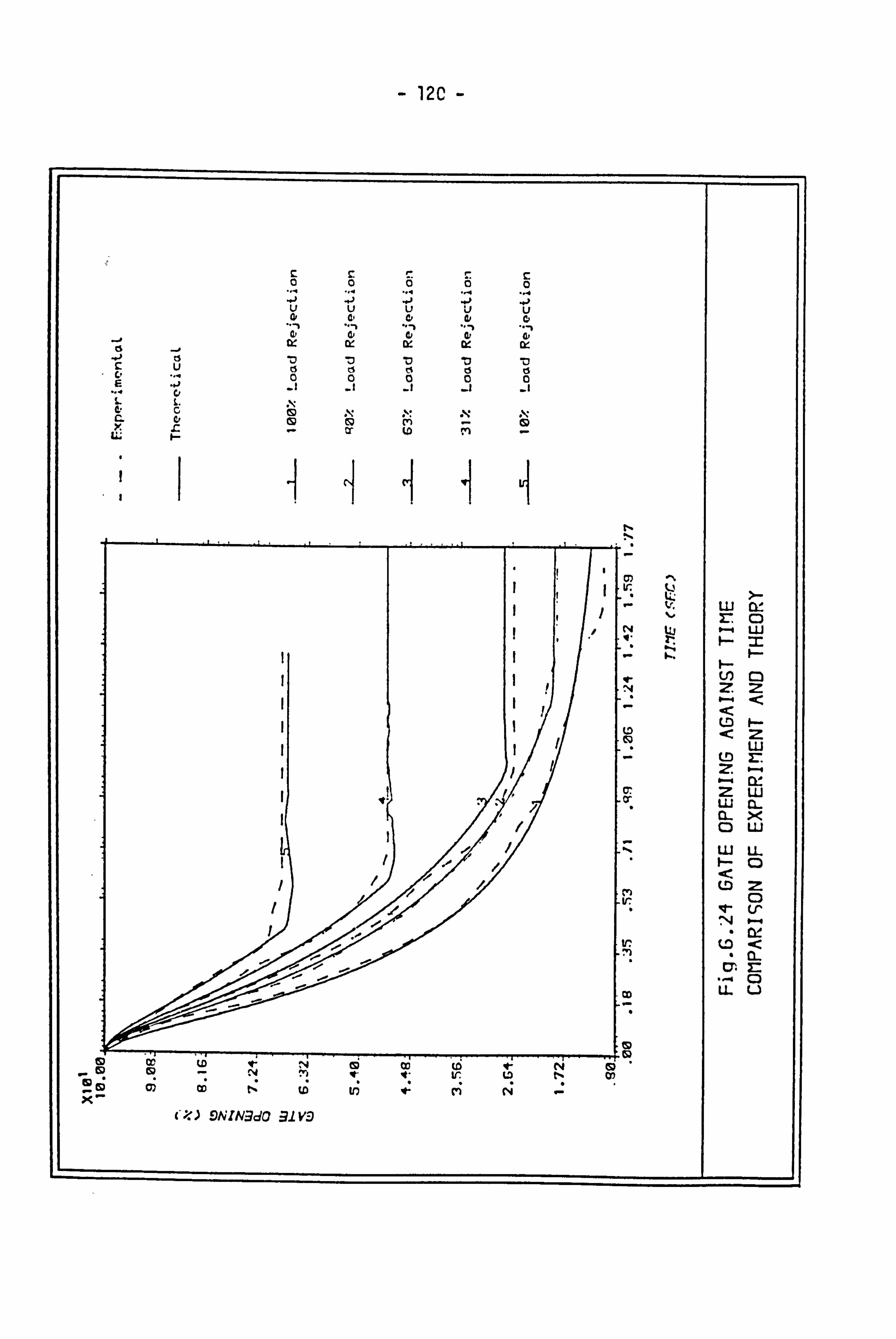
- 120 -

c 0 c 0 c 0 1.7 0

C 0

u u u Li u a- dp

ts 0: w w

0 15 0 d

cn N N

LL cr tD

Lr

LLI w Z. 0

N t1i f--q W

V) M Z. z

< LD < z

uj Lo Z-. Z

z LU uj CL CL X 0 ul Ul LL 1-- 0 U3 z

0 V- Lr ,4

tr Lo < CL

0 LL u

fs) (D co m to ir 0

OD t. 0 in

L L

i)A; rNgdo RIVE)

- 121 -

CHAPTER 7

CONCLUSIONS AND FURTHER WORK

7.1 CONCLUSIONS

In the literature survey in Chapter 2 previous computational work on studying transient problems in a hydraulic power unit governed by different types of governor and the governing stability was reviewed.

The work of this thesis is mainly concerned with developing a computer program using an improved interpolation technique to deal with the turbine boundary conditions making use of piecewise Lagrangean interpolation and designing and building a proportional plus integral

plus derivative (PID) governor to control a small turbine. It was found that the interpolation technique developed is more accurate than the other techniques and has many advantages which are explained in Chapter 3.

A model turbogenerator set was installed in the laboratory and a full range of tests were carried out both under full load and partial load rejection. In designing the PID governor it was found that a governor of the type described by Chaudhry, (Ref. 7), with linear elements was insufficiently stable for laboratory conditions because of the higher frequencies involved when working at the smaller scale. Hence a governor using second order elements was designed. Other points to note which were introduced to give satisfactory operation are:

(i) A phase-locked loop introduced to ensure that n and nref were in phase.

(ii) A smoothing network introduced to give approximated DC input to the step motor actuator.

The stability of the system was clearly illustrated by using the Bode plot method. Figure 4.7 shows that the-phase angle above minus 180 degrees means that the system is stable for all values of the frequency.

- 122 -

The computer program was described in Chapter 5. A flowchart for each part of the program and the main program has been drawn. The

program is flexible and uses all the points in the grid of the turbine characteristic curves (general Lagra

, ngean interpolation) or a specified

subdomain which surrounds the interpolation point and contains a certain number of the grid points (piecewise Lagrangean interpolation) depending

on the required accuracy.

Finally, a comparison between the computational and the experimental results has been described and presented with a plot for each test in Chapter 5. As can be seen there is a good measure of agreement particularly up to the peak of speed and pressure rise. However, the fluctuation in the experimental pressureltime curve, (Figure 6.4), was shorter and of smaller amplitude than those of previous researchers, (Refs. 3,7).

7.2 SUGGESTIONS FOR FURTHER WORK

1. The computer program developed for studying the transients

caused by load changes could be used for studying the transient behaviour when a fluctuating load is imposed on the system. In this case the power of the generator integrated with time would be used instead of the final generator power used when assuming a step change.

2. The PID governor presented in this thesis wa; 9 an. analogue governor. It would be worthwhile to develop a new digital governor, for example an adaptive control governor which changes the governor parameters with relation to the gate opening, and compare its result with the PID governor.

- 123 -

APPENDIX A

A. 1 PHASE LOCK LOOP

A typical connection diagram is shown in Figure A. I.

10 +12V 0'001 -r C2

INPUT V-,

SE/563 4 OUTPUT Vo 4 5h-o.

-

ci 1 ---10 -12 V

Figure A. 1

The voltage controlled oscillator (VCO) free running frequency is given approximately by

1.2 (A. 1)

and should be adjusted to be at the centre of the input signal frequency

range. Cl can be any value but Rl should be within the range of 2000 to 20,000 ohms with an optimum value of the order of 4,000 ohms, i. e.

The reference speed of the system = 2,000 rpm.

fN where P is the number of poles IT

fo = 2000

= 33.3 Hz 0-

Hence RI = 4,000 ohms :. -Cl = 2.2 PF

-ý 124 --

Lock range:

fL t8 fo

TC-C

where VCC -6 volts

:. fL = +44.4 Hz

Capture range:

fc 77-

'L

'r

I -I-

r

P--T

where -r = (3.6 x 10 3)xC2 and C2 - 2.4 UF

:. fc= +16 Hz.

(A. 2) .

Practically it was found that the capture range is = +20 Hz.

A. 2 PROPORTIONAL ELEMENT

R2

VO

Figure A. 2

In Figure A. 2, the circuit inverts the polarity of the applied input signal but the gain of the feedback circuit is determined by the value of the external elements. The following relationships are established.

The current supplied by the-input signal is:

'in . Vin

R- Vf

I

125-

since Yf is virtual earth i. e. Vf -0

in ' Yin 71-

The effective nput resistance of the circuit Is thus Rl. The

output voltage causes If to flow through resistor R2 and

lin+l f=I

since Zin 0`

:. IT=

lf

Vin In f

vo R-i 1Z2

R2 vo In

where R2/Rl = Kp, the gain of the proportional elements.

A. 3 INTEGRATOR CIRCUIT

The basic diagram of the second order system is shown below.

u

vi

Figure A. 3

- 126 -

III = IYIIVI

y 11 Y12 Y13 y 14 Y21 y 22 y 23 y 24 y 31 Y32 y 33 y 34 Y41 y 42 y 43 y 44

1 y

2 -Yi

34 001

-Y I yI +y 2 +y 4 -Y2 -Y 42

0 -Y 2 y2 +y 303 0 -Y4 0y44

The gain of the operational amplifier is very high and the output is limited, i. e. the input voltage = 0.

Column 3 can be added to column 4 and since the output impedance of the operational amplifier is equal to zero row 4 can be can- celled.

The input impedance Z All in a

The output impedance Z A44 0A

i. e. the transfer function is

z0x10 '7- 'Tin

in

A14 x (-1) 1+4 AS-TT

A14 =Y1Y2 (i. e. by deleting row I and column 4)

All = 1(y 1 +Y 2 +Y 4)N'ýY33 - Y2(y2+y4)1

- 127; -

All =y IY2. +y 1ý3-+ y2y3 + y4y3

H-- -1 (S) yy+yyy

+ 1.3 32+43

yl Y2. -

T172

YlY2 should be independent of frequency, i. e. resistors.

Yl -I and Y2.

Y3 = SC 3 Y4 = SC4

H -1 (S) I+ sc 3(R, +R 2) + S; ý(R, R2C3Y

But the general transfer function of second order systems is: -

K0

s+I sz 0 wo

21 wn " RIR2C3E; 4

For simplicity R, =R2=R C3 =C4=C

.. Wn - lw

and 2r. = C3(R, +R21

wn

Rr' = 2RC

wn

:. &=I

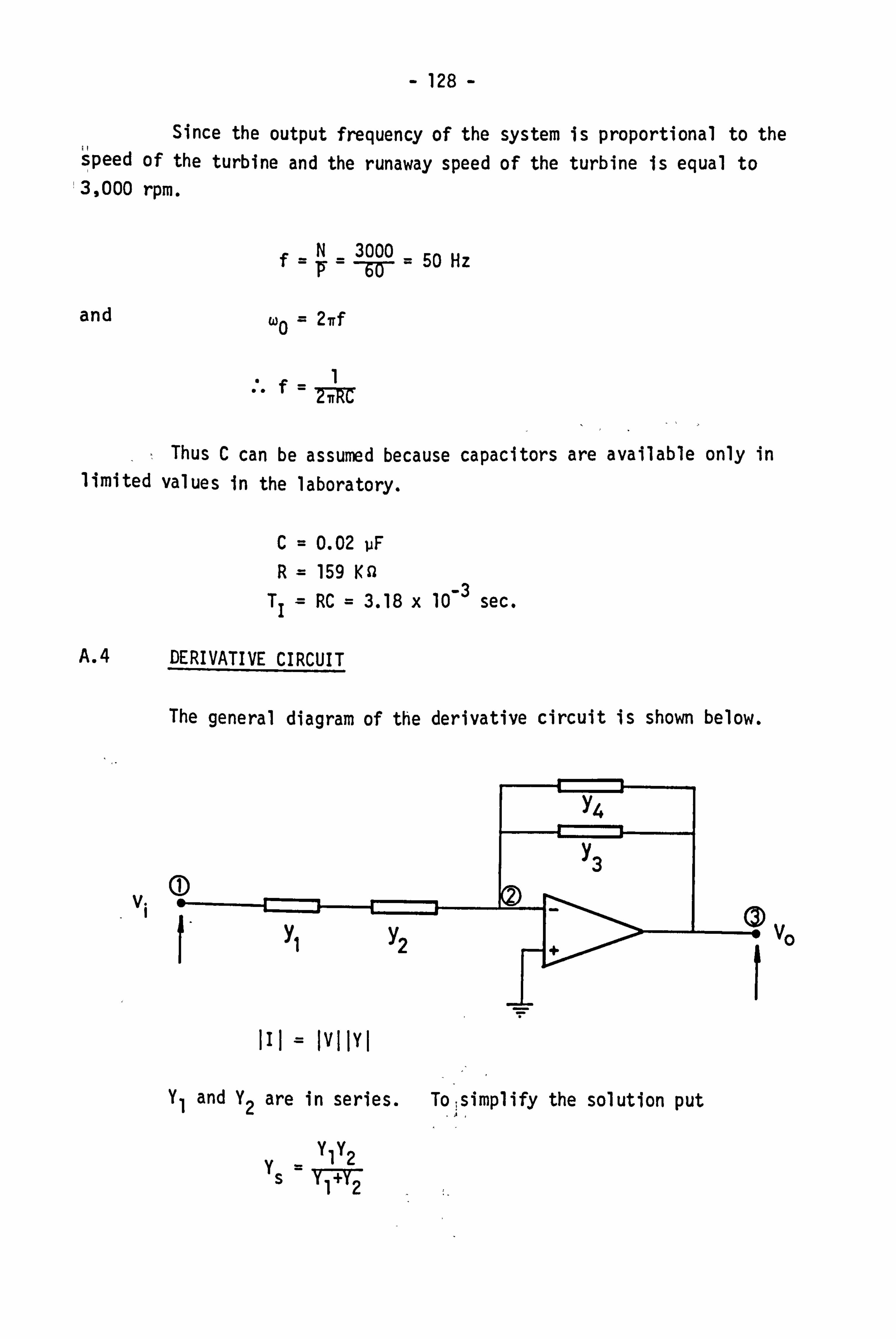
- 128 -

Since the output frequency of the system is proportional to the speed of the turbine and the runaway speed of the turbine is equal to 3,000 rpm.

f -- N 3000

= 50 Hz

and wo = 27rf

ZwRL

,, Thus C can be assumed because capacitors are available only in

limited values in the laboratory.

C=0.02 laF R= 159 Kn

TI= RC = 3.18 x0 -3 sec.

A. 4 DERIVATIVE CIRCUIT

The general diagram of the derivative circuit is shown below.

vi VO

III = IVIIYI

Y, and Y2 are in series. To, simplify the solution put

y YlY2

y7r2

- 129 -

y 11 y 12 Y13

y=y 21 Y22 y 23

. Y31 y 32 Y33

123 ys -Y s01

-Y y +y y (Y5Y )2 ss 3+ 44 o -(y 3 +y 4) y 3+y 43

Since the output impedance of the operational amplifier is

equal to zero, column 2 and row 3 can be deleted.

ys

_YS -(Y 3 +y 4)

Similarly the transfer function is

H A13 1+3 (S) ETT (- 1)

and -Y 1y2 A13 =-Y s=y1 +Y 2

All =-(y 3+y 4)

H (S) - (y +Y YlY2

+7- 1 2) (y3+ 47

where Yy= SCI 9y=I, Y= SC 23 IFý 42 2

HR2cIs (S) 1+I (Rc 1 +R 2c 2)S +(RIR 2CIC2 )ý2

For simplicity take R1C1R2C2=TD

and R 2CI KD

- 130 -

H KDS

Sý 1+ 2TDý. + T DSZ

v D(S) K Ds z (S) I+ 2TD +s S TB

Hence f=1 0 2vR C

if C, = 1.0 PF ýR, = 3.18 Kn TD- 3.18 x 10 -3 sec.

Also

C2' = 32 nF

-R2 = 100 Kn

A. 5' SMOOTHING NETWORK

This is a second order low pass filter.,,, The derivation of a second order system was shown in Section A. 3. It was found that an approximated DC output can be obtained'when'wo = 10 Hz i. e.

Referring to equation

f- WO

f Z7rRG

Similarly C can be assumed e. g. C 0.47 pF.

R=33 Kn

TA = 0.015 sec.

131

APPENDIX (B) 49* ge 49 0q

EXPERIMENTAL RESULTS

C*** FULL LOAD REJECTION 100% *** C*** FINAL isENERATOP LOAD PG=0*0 C49*49 RATED 61EAD HNz2l*O CIO C*** SYNCHRONOUS SPEED NR=2000.0 RPM

TIME USEC)

*V: - **U; c****

0.00000E+00

0.10000E+00

2n. DC05+00

0.30000E+00

0.40000E*00

O. tOOOOE+00

0.70000E+CC

0.60000E+00

0.90000E+CC

CelOOODE+01

00110005+01

Dol? DODE+01

0*13000E+01

0*14000E+01

0*15000E+ol

0*16000E+01

0*17000E+ol

SPECD NCRPM)

3xv a* rA *VC kt 4c

0920000E*04

0*21700E+04

0.23130E+04

0.24000E+04

09'44650E+04

0.25000E+04

0925200E*04

0.25330E+Oý

0.25530E+04

0.25750E+04

0.25650E+04

0*25550E+04

0-2530CE+04

0.25270E*04

0*2blBOE+04

0.24990E+04

0*24800E+04

Do24720E+04

FLOwRATE C(1/5)

O. lzoOb6E+02

0.122955+02

0*985STE+01

0*80960E+01

0.65052E+01

0,54T16E+01

0,48631E*01

0.40903E+01

0*-29487E+01

0.34332E+02

0.33022E+01

0.2: ý747E+01

0.23575E+01

0920743E+01

Ool7910E+01

0*17910E+01

0.17910E+01

0*17910E+01

HEAD RISE PRCM)

O. OOOOOE+00

0011156E+01

0.26396E+01

0.29779E+01

0*35538E+01

0.37271E+01

0.40802E*01

0,43891E+01

Oo4Zo4lbE+D1

0*46939E+01

0, *48158E+Dl

0*49073E+01

0.43282E*01

Oe45720E+01

0*42672E+01

Oo42062E*01

0*41148E+01

0ea9624E+01

GATE OPENINS M

*V1*vc;; vc4c***4c 0*10000E+03

Oo89436E+02

0*69813E+02

0*561276+02

0944625E+02

0.3662. -)E+02

Oo3l938E+02

0*27812E+02

0.252bOE+02

0*21250E*02

0919450E+02

0918220E+02

0*16250E+02

0*15250E+02

0-14550E+02

0*11250E+02

0*10000E+02

0*10250E+02

132 -

Cw 49 49 PARTIAL LOAD REDUCTICN b0% *** C*** FINAL GENEkATUR LOAD PGx0o44 KW Cg; ** RATED HEAD HNz2l*O Cv) C*vc*c SYNCHRONOUS SPEED NR=2000*0

T2 04 E T(SEC)

99 w4c * 39 *4tv 9 *C

DolOODOE+00

0.20000E+Co

0.30000E+CC

0.40000E+00

0.50000E+00

OofODDDE+00

0.70000E+cc

0.60300E+oo

0.90000E+00

0. '20000E+01

0.11000E+01

0.12030E+01

0.13000E+01

0*14000E+01

0*1ý000E+01

0.26000E+01

0.27000E+01

SPEED N(RPM) **gc* *49M 4

0.20000E*04

0*21700E*04

Co22750E+04

0*23500E+04

0*239bOE+04

0.24300E+04

0.24500E+04

0,245c. OE+04

0.24430E+04

0*24230E+04

0*24000E+04

0.23P5CE+04

0.23600E+04

0*23250E*04

0.23000E+04

0*22750E+04

0.22450E+04

0.22300E+04

FLOWRATE Q(I/S) 31C ********

0.15038E+02

0.13310E+02

0,11045E+02

0.90624E+01

0.76464E+01

0.65835E+01

0.600EB'E+01

0'. 4: 7144E+01

0944096E+01

0.39648E*01

0.3 8 0-32 E'+O 1

0.33784E'+01

0.32984 E+O1

0-33084E+01

0932884E+01

0.33484E+01

0933E84E+01

HEAD RISE PR (, M)

O*OOOOOE+00

0.11887E+01

0.22250E+01

0.28224E*01

0.32918E+01

0.35965E+01

0.39319E+01

0.40843E+01

0*42367E+01

0.39319E+01

0*40843E+01

0.39624E+01

0*38710E+01

0.36576E+01

0.33528E+01

0.3017. rE+01

0.27432E+01

0.24384E+01

GATE OPENING M

0.10000003

0.90000002

0.75300E+02

0.62000E+02

0.54000E+02

0*45300E+02

De40000002

0*34000E+02

0*30000E+02

0*26200E+02

0*24000E+02

0*22000E+02

0*21000E+02

0.20000002

0*18500E+02

0.18500E+02

0*18500E+02

Oele5OOE+02

.- 133-

Cw*qc PARTIAL LOAD REJECTION 63% *** (49*c* FINAL GENERATOR LOAD PGuO*9 KW C*4%w RATED HEAD HNz2l. D (m) C**: *- SYNCHRONOUS SPEED NRz2000*0 RPM

TIME, - Tcs; -C)

*xc *it *3x* *

0.00000E*oo

0.10000E+00

0.20000E+DC

. 30000E+00

0*40000E+00

O. -cDOOOE+Co

OobDOOOE+DC

0.70000E+00

0.60000E+00

0.90000E+00

0.10000E+01

0921000E*01

Ool2OOCE+01

0.13000E+ol

D. ls-OOOE+01

0*15000E+01

Ool6OCOE+01

0*27000E+01

SPEED N(RPM)

Oo2O3205+04

0.21850E+C4

DoZ2760E+04

0.23460E+04

0.23800E+04

0.23990E+04

0923890E+04

0.23760E+04

0.23500E+04

0*233COE+04

Oo23000E+04

0.22600E+04

0.22140E+04

0.21780E+04

0,21450E+04

0.21000E+04

0,20860E+04

Co20550E+04

FL: )WRATE QCI/s)

39VE39 * *** 49 **

0.14986! +02

0.13092E+02

0.11359E+02

0*97449E+01

0*86724E+01

0971681E+01

0.63468E+01

Oozi9O76E+01

0.53213E+01

0*50410E+01

0*47861E+01

0*43924E+01

0943301E+01

0,43046E+01

0*43046E+01

Oo43046E+01

0,43046E+01

0*43046E+01

HEAD RISE PR ( -. w)

*** * qt *

0.00000E+00

0.7S029E+00

Oel9507E+01

Oo24689E+01

0*30785E*01

0.32736E+01

0.36119E+01

0.36881E+01

0.38283E+01

0.35357E+01

0.33833E+01

0.3109DE*01

Oo29870E+01

0.26822E+01

0.23774E+01

0.21031E+ol

Ool7678E+01

0.12497E+01

G OATE OPENING

**#3X** ** Ovtvc *t

D. 10000E+03

0.9137b5+02

0978112E*02

0.66250E+02

0.5zo7. j0E+02

094e00DE+0&

0943120E+02

0*36000E+02

0.30125E+02

0.28120E+02

0*26250E+02

Oo26240E+02

0.26260E+02

0.26260E+02

0*262bOE+O&l

0,26260E+02

0*26260E+02

0,26260E+02

- 134 -

CIP** PARTIAL LOAD REJECTION 31% *** Eý** FINAL GENERATOR LUAU PGal.: 5 KW E*Iciw RATED HEAD tiN*21 Cm) [I**

- SYNCHRONCUS SPEED NR=2000*0 RPM

TIME TC S EC)

0. Of' 000 E+00

0o ICIOODE+00

00 20000E+00

. J. 1 -, - 0 0,3 0000E+00

1) 11000'DE+00

00, C1000E+00 0,

0 60000E+00

7110 00 E+ 00

SCIOODE+00

0*90000E+00

0-10000E+01 ill -IIiI 0.11000E+Ol 11 1ý,., 0.12000E+01

Ool3OOOE+01

0.14000E+01

0*15000E+01

SPEED N(PPM)

******vc* 0.2nOODE404

0*21200E+04

0*21600E+04

0*21950E+04

0.22000E+04

0.22200E*04

0.22930E+04

0.21700E*04

0.21450E+04

0.21200E+04

0*20850E+04

0*20680E+04

0.20: 5! )OE+04

Oe20510E+04

0,20480E+04

0920460E+04

FLOwRATF Qcl/s)

0.15083E+02

0.13772E+02

0*12065E+02

0.10643E*02

0*93966E*01

0,64646E+01

0*79296E+01

0977314E+01

0*75898E+01

0.7.3504E+01

0973066E+01

0973066E+01

Oo73066E+01

0.73066E*01

0.73066E+01

0*73066E+01

Ool6OOOE+01 0920460E+04 0.73066E+01

HEAD RISE PRCm)

O. OOOOOE+00

0.67056E+00

0*14021E+01

0.22336E+01

0.23TT4E+01

0*2T432E+01

0928651E+01

0926213E+01

0.22250E+01

0.15240E+01

0.12192E+01

0.91440E+00

0.60960E+00

0.304eDE+00

0.27432E+00

0,27432E+00

GATE OPENING M

0*10000E+03

0.92800E+02

0.60920E+02

0.73180E+02

0*62250E+02

0.55500E+02

0,51100002

0.49000E+02

0*49000E+02

Oo49000E+02

0-49000E+02

0*49000E+02

0*49000E+02

0*49000E+O&

0*49000E+02

0*49000E+02

D*4900DE+02

CV** PARTIAL LOAD REJECTION 10% *** C*lw4c FINAL GE14ERATOR LOAD PGx2el KW C*** RATED HEAD HNz2loD (m) CIF** SYNCHRONOUS SPEED NRz200DeO RPM

TIME T(SEC)

DoOVDDOE+OC

0*10000E+00

0*20000E+00

0.30000E+00

0.40000E+00

OoSnOOOE+00

0.60000E+00

0.70000E+00

0.6000ce+oo

0.90000E+00

OeICOOOE+01

0.12000E+01

0.12000E+01

04,13000E+01

0.14000E+01

SPEED N(RPM)

C. 20200E+04

Oo2D! )ECE+04

0.20730E+04

0.2073DE404

0*20600E+04

0.20! 60E+04

0*20160E+04

Oo2O2OOE+04

0920200E+04

0.20200E+04

0.20200&+04

0.202002+04

0*20200r. -+04

0.2020CE+04

0.20200E+04

FLDWRATE

0*24885E+02

Dol3982E+02

0*1302TE+02

0.11894E+02

0.10895E+02

0*10563E+02

0.10478E+02

0.20337E+02

0.10195=-+02

0.10195E+02

0.10195E+02

0.1019SE+02

0.10195E+02

0.10195E+02

0.10195E+02

HEAD RISE PR(m)

0*00000E+00

0960963E+00

0*97536E+00

0.13411E+01

0.17374E+01

0*16490E+01

0.1! M1E+01

0.13105E+01

0.10058E+01

Do67056E+00

0.30528E+00

0.15336E+00

0*6096DE-01

0.36576E-01

0.365TSE-01

GATE OPENING

0.10000E+03

0.9300CE+02

Do86DDOE+02

0.78000E+02

0.70500E+04'

Oe69500E+02

O. bSOOOE+D2

0*68000E+02

0968000E+02

0.68000E+02

0-68000E+02

0*68000E+02

0*68000E+02

o. o8DDOE+02

Oo6FOOOE+02

136 -

APPENDIX CC)

INITIAL CONDITION DATA

6o 4.32*2 1104*0 0*0 20009 0.531 70*0 OoOlS 0-0015

0*987874319 0*0 0,96 0*00318 1.2 0*015 0.00318

1200 Oo27899999 Oo78O34512

1*0 0.6 0*0023 0.27 OoOI73 0*47 0-02

10 0.0 000 000 1.

1.

9-5 1.0 16 lo6

**** TURBINE CHARACTERISTIC DATA ***

UNIT SPEED VS UNIT FLOW DATA

NU4BER OF GATE OPENING

4

0*2500000 0.5000000 017500000 1.000000

NUMBER OF UNIT SPEED VS UNIT FLOw PONITS

10

UNIT SPEED UNIT FLOW

0.1011900 001080700 0*1762800 0*1080700 0.2529900 0.1080700 0*3525600 0.1070000 0*4765500 9.6439999E-02 0.6855000 9.415999SE-02 0*7932000 8,5599996E-02 0*84870DO e, 0250002E-02 008911boo 7.4900001E-02

m 137 --

0*9466801 6.74100DOE-02

14

8*1615001E-02 0.1819000 001550550 0.1POE300 0.2285100 0*1797600 0.3100: 00 0.17elbjO 0.3917250 0.1765502 0*4b9600 0.1733400 0.5875950 0,1679900 0*7181700 0.1.562200 0*7998000 0.1465900 098846551 0.1348200 099287250 0.1273300 0.9562700 0.1187700 1.002150 0.1223500 10031550 0.1016500

17

8.16150DIE-02 0.2430556 0.1632000 0.2350500 0.3231750 0,4015500 0.4815000 0*5451600 Oo6349500 0*7 018.5 00 0*7704000 0.8586000 0*9060000 0*9630001 0*9956400 10028250 IoO54500 1.0837! iO

092396800 0.2396101 0.2364700 0.2354000 0.2327250 0*2300500 0.2257700 0.2193500 0*2107

* 900

0.1979500 0.1872500 0.2722TOO 0*2626400 0.1524750 0.1433800 0.1316100

17

0.1060950 0.1926000 0.2774745 0*3623505 0*4570200 0*5549505

0*3081600 0*3060200 0.3049500 0.3038800 Oo3006721 092974600

---138-

0.6153427 0*7018500 0*7834050 0*8487480 0.9271500 0-9793260 1*028295 19051140 1.0772be IoO96875 1*1131b5

0.2942500 0.2889000 0.2803400 0*2717800 0*2546600 0.2396800 0.2268400 0.209T200 0#19toso9e 0*1829698 0*1690600

----------------------------------- UNIT SPEED VS UNIT POWER DATA

NU4BER. DF GATE OPENING

6

002500000 0.5000000 0, T500000

4UMBER OF UNIT SPEED VS UNIT POWER PONITS

10

UNIT SPEED UNIT POWER

001011900 OeIT62600 0.2.529900 0*3525600 0*4765500 0*6855000 0*7932000 OeB487000 0.8911600 099466801

14

8.16150DIE-02 0.1550550 0.2285100 0.3100500 0.3917250 0*4896600 Oo5875950

1*2475353E-03 2.4950707E-03 3.7426064E-03 4,9407338E-03 5,6818440E-03 5o4348069E-03 3-952587SE-03 2.7791630E-03 1.7292569E-03 7.7816559E-04

2,0998120E-03 4ol749203E-03 6*2253247E-03 8o2263229E-03 1.0190264E-02 1*2005984E-02 1.2605048E-02

1*000000

-:. 139 -

0*7161700 0,7998000 OeSS46551 0-9287250 ()*96627DO loOD2150 1*031550

17

8.1615001E-02 0.1632000 Oo2350500 0.3232750 0.4015500 0.4815000 0*5451600 Oo6349500 Oo7018500 0*7704000 0.8586000 Oo9360000 Oo9630001 Oo9956400 1.028295 IoO54500 1.083750

17

OoID60950 0*1926000 092774745 0.3523505 0.4570200 0*5549502 0*6153427 0.7018500 0.7834650 0,8487480 0*9271500 0*9793260 1'028295 1: 051140 1*077258 1*096845 1*113165

1*1721891E-02 loOIS3209E-02 7.7816565E-03 5.8794734E-03 4,113161SE-03 2o5938954E-03 lol734243E-03

2.779163DE-03 5.5336226E-03 8.2633775E-03 1.0919022E-02 1*358701SE-02 1*6229147E-02 2*7261691E-02 1*8243661E-02 1*8099729E-02 1.7033182E-02 1*4853082E-02 1.2969427E-02 9*9432273E-03 7.5099203E-03 5*2604099E-03 3*3102920E-03 1.51927ýo7E-03

3*5573286E-03 7oll46232E-03 1*0560819E-02 1.403168SE-02 1*7354328E-02 2.060286IS-02 2.207890SE-02 2.3344969E-02 2.3138694E-02 2ol961564E-02 1.9108290E-02 19660086BE-02 1.3092945E-02 9.68383BIE-03 6*7811576E-03 4o2243279E-03 1*9515899E-03

- 140 -

APPENDIX D

IDA Derivation of equation (5.6).

Let I i(X) , Yr = X-xr

. x. j-xr

and zý YI Y2 Y3*****Yr

X-xk Yk X--x 4k

Then log z= log y, + log Y2 + log Y3 '****" + log Yr

Differentiate both sides of the equation with respect to x.

az i lyl 1 aY2 +1

aY3 +1

ay r ý -x Tl ax

+ Y2 ax Y3 ax ----- Yr ax

Multiply both sides by z and let dy/dx = y'

az a7 yi Y2 Y3 Yr + YI yi Y3 Yr + yl Y2 4 Yr

yl Y2 Y3 '*** Yr,

m Hy X

r=l r

mm ýyk Yd j-x kil

(rýll

rik

But ýk X-xk

Xj-xk

3yk 1 and ýx "xj-xk

m X-X (X) r ax

J1 (7j-xK) r=l

YX r

kýj rA rik

(5.6)

' 141 - D. 2 Derivation of equation (5-7).

By the previous method the second derivative of equation (3.43) can be derived.

Then

a at i (X) mIam X-X

TR % ax )x---C 11 )) I

(T-X, r= xj-'r k= jk

ýx I

kOj rOi rik

Substitute equation (5.6)

a2Li (x) ,1mm x-xr

j Xt) x 2 ax t=l Z ký( xi xk' r=l i Xr

. toi kOi rOi k0 rOk

r09

(5.7)

- 142 -

c*# APPENDIX E C 3gg *4c3gwvc4c; c4c* 0 *v* *****

c

c TRANSIENTS CAUSED BY LOAD CHANGES ON c TURBCGENERATOR SET C, C* C c

PROGRAM MAIN

C. C, NuRCTATIONAL SPEED (RPM) NR=PATED SPEED (RPM) C AREA-CFOSS-SECTIONAL AREA OF PIPE (M**2) C A=WATERHAMMEP WAVE VELOCITY Cm/s) D-PIPE DIAM- C ETEP (m) DP-TURBINE RUNNER DIAMETER Cm) FzDAR- C CY-WEISzACH FRICTION FACTOR GzACCELERATIDN DUE TO C GPAVITY CM/S**2) n=N/NR PHIzUNIT SPEED QI=UNIT FLOW C PxUNIT POWER PG=PDWER DF GENERATOR CKW) ETASaGENERATOR C EFFICIENCY SEGMA=PERMANENT SPEED DRDOP NTAUaNUMdER OF r %, GATE OPENING CURVES FROM TURBINE CHARACTERISTICS C NPHI=NUM8ER OF UNIT SPEED MAzPIEZOMETRIC HEAD AT C BEGIVING DF TIME STEP HN=NET HEAD(m) HP=PIEZOMETRIC C HEAD AT END OF TIME STEP HT=TAILWATER LEVEL ABOVE TmE C DATUM (m) II=MOMENT OF INERTIA DF ROTATION AL PARTS C (KG*M**2) &D=GAIN OF DERIVATIVE ELEMENT KEi-VCLTAGE C CONSTANT DF STEP MOTDR CVLLTS/RADIAN) KlzMAGNETIC NULL C DISPLACEMENT CONSTAN DF STEP MOTOR (RADIANS/AMP) C KM=CDNSTANT OF ANALOGUE MULTIPLIER KP=GAIN OF PRDPOR- C IONAL ELEMENT QAzFL0W AT BEGINNING OF TIME STEP (1/s) C QPcFLDw AT THE END TIME STEP (1/s) C RuRESISTANSE OF STEP MOTOR WINDINGS TAuSMODTHING NET- C WORK TIME CONSTANT TDzTIME CDNSTANT DF THE DERIVATIVE C ELEMENT Tl=TIME CONSTANT DF THE INTEGRAL ELEMENT C, TS=TIME CONSTANT OF STEP MOTDR WINDING VA=SMDOTHING C NETOORK OUTPUT VDwOUTPUT OF DERIVATIVE ELEMENT Vla C DUTPUT OF INTEGRAL ELEMENT VPzOUTPUT OF PRDPDRTIONAL C ELEMENT Z=INPUT TO DERIVATIVE91NTEGRAL AND PRDPORTIONAL C ELEMENTS NPAzNUM5ER OF PARTS INTO WHICH PIPE IS DIVIDED C V*vw; eq*; c 0*

REAL NqNRqYA(6) COMMON /RC/NR/RUNGEC/NTIMEtDTtY(6)tDYC6)/INITIALC/YREFC6) COMMON/ITERC3/LIPAC100)tHPA(100) CHARACTER* 3 CASEoFN*19FILE*7 READ(1v'(A3qIX9Al)') CASEqFN IFCCASE*NE. 'NEW'*ANDeCASE, NE. 'CLD*) STOP 'UNDEFIND CASEI' FILEz'MP'//FN//'*PLOP

- 143 -

IF(CASE. EQ. 'DLD*) THEN OPENCl4tACCESSr-*UIPECT'tRECLu6DtNA4EwFILEPSTATUS*'DLD'g

x FOP A! = OF OR MATT ED) READC149'(15)*qPECýJ) IPEC CALL DATA(l) READC559RECul) T9ITqQPqPHIIqHNqHPqYqDyqCPqYN READC! 5qRECz2)WPA READ 9REC z3)HP A GO TO 80 END IP LPENC149ACCESS='DIRECT09RECL=609NAME=FILEgSTATUS='NEW*g

x FOFMw'FClRMATTED') WP'&TE(149'CSE12*5)'tRECulODD*)O. OgOoOtO. OtD. Ogo. O I P. E 1. =I T=0.0 IT=0 CALL OATA(fWl) 6PITE(2930) W7'LTE(2v. -)0)Y 00 70 1=196

70 Y4(I)=YFEF(I)*Y(Z) 6; -ITE(295C) YA

so 00 10 Il=lvNTI-4F T=T+DT IT=IT+l NzNA-, -tYCl) TAUI=Y(6) VY; EF(6) CALL ý'TEPCNtQPtTAUIPPHIIgHNgHPPITtPRtCPtYN) WkITE(2v60)IT-19T-DTqNvQPqHNq"P

C Wk. 'LTE(2960)IT-19T-DTgNtQPgHNoMP IFCC(IT-2)/1V)ml0. EQ. IT-2) THEN IREC=ýIREC+l WkIT=-Cl49v(5cý12910)'gRECzIREC) T-DTtNPQPtPk*Y(6) END IF END IF CALL RUf. 6ECPflII9TAUIqHN)

WRITEC295O)Y C- WRITE(2950)Y

DC 75 1-196 75 YA(I)=YkEF(I)3v-Y(I)

IF(((IT-1)/10)*10, E%r*IT-1) WRITE(2950) YA c WRlTEC2950)YA

IF(Y(6). LT*C*O*DR*YC6)eGT*I)STOP'TAU OUT OF RANGE' 10 CONTINUE 1 30 FOP4ATC3XP'lTgTtNtQPtHNtHPtN/NRgVIgVAtVDgVPoTAU: '/) so FCRMAT(6Dx96Gll. 4) 60 FOR4AT(lH+qI4q6Gllo4)

WFITE(5., ýqREC=l) TgITtQPgPHIIPHNgHPgYtDYtCPtYN WRITE(559PECuMPA WRITE(5! 9RECu3)HPA

- 144 -

W; ITE(14q'(I5)'qREC=I) IREC STOP'CoKe' END

SUt3RC, UTINE DATP (IDATA) COMMON/INITIALC/YREFC6)tSSGMA REAL NRoNREFgKPolloKtKMgLtKlgKEoMCgNCtKD CC14MON/TAUC/NT4LIoTAU(40)/PHIC/NPHI(40)#PHI(4094C)

1 /ITE; C/HTtSO9S29S29S39S49S59S6/RC/NRgWAtRl9R29P39HAtHAA 3 /DEC/EOtElktKvKMtNREFPTCgTlgTAgKPtMCgNCtKD 4 /RUNGEC/NTIMEgOTtYC6)90YC6)tPOINTS/Q(40940)tP(40940) 5 /ITERC2/S7qNPA9APEA9A9C9HS

READ C 10 9 xc) f; TAU READC10q3%)CTAUCI)qlmlvNTAU) DC 10 Irlot. TAU REAOCjGq*)NPHI(l)

10 RýAD(109*)(PHI(Igj)tg(IgJ)gJclgNPHICI)) PEA X20, kc) NTAUZ IF(NTAU2. NE, NTAU)STCP'CHARTS DATA ERPOR' READ(ZCs*)CTAU(I)qjwjqNTAU) UO 20 1=19NTAU READ( 2C90NOH I( I)

23 kEADC209xc)(PHI(19J)gP(IgJ)gJzlgNPHICI)) IF(IDATA. EC. 1)GO TO 50 OPEN(559ACCESS= 'DIRECT'q STATUS= 'NEW'gRECL=100) WýITE(2922) F0R4AT(/5Xq'DATA PARAMETERS'/SX915(lH-)) READ(19*)DRPDgGgAoHTgNRgQAgHAtFgDT P142ATANI(1,0) AREA=P 14 VcD ve D/ 14 4, Rl=(DR/12*)**Z S0mF3xDT/(2. *AR5Aw0/12. ) S18G*AREA/A S2=0*5/AREA/A S3=DR/1636. S4=Io0/P1 S5xDR*v3/lb38, /144o

G/AREA**2 S6z0*5 IV R2zDR**3*NR/264672. R3w(Rl3ýKR)**2/23460* READ(19*)119PGttc. TAGPT19KPoTAgTDtKD kEAD(19*)NTIME9L; INqPHIIN READ(1qv)KqKM9LpRqKIvKEqSEGMA MC=(L+KE*KI)/R NCxKI/R EOa9l*l9*b'ýKCoO*32*2/II/CNR**Z) ElRxEO*PG/ETAG TAUINzTAUF(PHIINqQIN) NkEFuloO

- 145 -

C INITIAL AND REFERANCE VALUES kEAD(I9*)(YREFCI)9Iz2q6) READ(l949)CVCl)9lzl96) REA3(1q*)CqlSqNPAtDX

YF5F(6)zTAUIN DY(I)MO. 0 DY(5)=O, C 0y(6)c0. C DY(2)=DY(Z)*DT DY(3)=DY(3)*DT DY(4)zDYC4)vDT YAEF(I)aNP WRITE( -)Cg 30 YPEFjSEG2MA WRITE(509*) HT9SOqSlqS2qS39S4qS5qS6qS7 WPITE(. 509*) NF9CAqRl9F2qR3tHAvHAA WRITE(509*) EOgc-lRtKgKMtNREFgTDgTIgTApKPgMCoNC WRITE( 509 30 NTIME90T WPITE(509*) CqHSqNPAqDX PETURN REAO(., 09'X) YREFgSEGMA PEAC(5090 HT#SOtSl9S2tS39S4qS5qS6qS7 REAO(509u) NRqQA#Rl9R29R3#HA9HAA READ(509w) EOgElý-gKgKmpNREFgTDgTlgTAtKPtMCgNC READ(: oOqix) NTIMEtDT READ(50or-) CqhSqNPAqDX P ETURN END

PUNCTION F-ACT(lqJqKqLqPHIQ) COMMON/PHIC/NPHI(40)tPHIC40940) INTEGER P FACT=, ' 00 10 Rzitt., Ptil(l) IF(Ooc-QeJoCR*R*ECoK. OP*R. EQ*L)i^aD TO 10 FACTzFACT*(PtiID-PHI(19R))/CPHI(19J)-PHI(IgR))

10 CONTINUE PETJkN END

FUNCTION FLAG1(NgXgIgXO) DI4ENSICN X(N) INTEGER R FLA'%Vl =1 DO 10 R=19N IF(R. NE*I)FLAGlaFLA. 'I*(XO-X(R))/(X(I)-X(R))

ID CONTINUE RETURN END

- 146 -

FUNCTICIN FLAG(IqJqPHIO) FLAG=FACT(I9JqOjOqPHIQ) A E. - TURN END

FUNCTION VLAG(IqJjP4I0) COMMO? 4/PMIC/NDHI(40)tPHI(40940) DLAW'31=0.0 DE) 10 KzlttiPm'. '(I) IF(K. N--,, J)OLA'o'=DLAG+FACT(IpJtKgDgPHIO)/(PHI(IgJ)-PHI(IgK))

10 CONTINUE END

FUNCTION 02LAG(IqJqPrlIO) COP-MON/PHIC/NPHI(40)tPHI(40940) Dd'LAG=0.0 00 20 Kal, NPHI(l) ll; '(K*"Q*J)GO TC 20 s=000 DO 1C LzlqNPHl(l) lF(L*5'bf. J. Cl? *L. EL, K)GO TO 10 S=S+FACT(IgJgKgLgPHIC)/(PHI(19J)-PHI(19L))

10 CONTINUE L)ZLAG=DZLAG+S/(PHI(Igi)-Ptil(19K))

20 CONTINUE RETUPt., r- N0

FUNCTION TAUF(PHIItUl) CCM40N/TAUC/NTAUtTAU(40)/PHIC/NPHI(40)/PDINTS/C(40940) DIMENSION Y(40) DO 50 1=19RTAU Y(I)vo. 0 DO 50 Jzl*NPHI(l)

50 YCI)=Y(I)+Q(IPJ)3ýFLAG(IgJtPHII) TALIF=C*C 00 100 I=IgkTAU

I'vo TAUF=TAUF+TAU(I)xFLAGlCNTAUtYtltQl) RETUAN END

PUNCTION ZI(TAU19PHIItZPID) 014ENSION J(40940)qY(40) COMMON/TAUC/NTAUgTAU(40)/P41C/NPHIC40)

C*** PIECEWISE LAGRANGEAN INTERPCLATION DO 10 1 =I 9 NTA U IP(TAUI*LT, TAU(I)) GO TO 20

ic CONTINUE hIzNTAU-1 GO TO 30

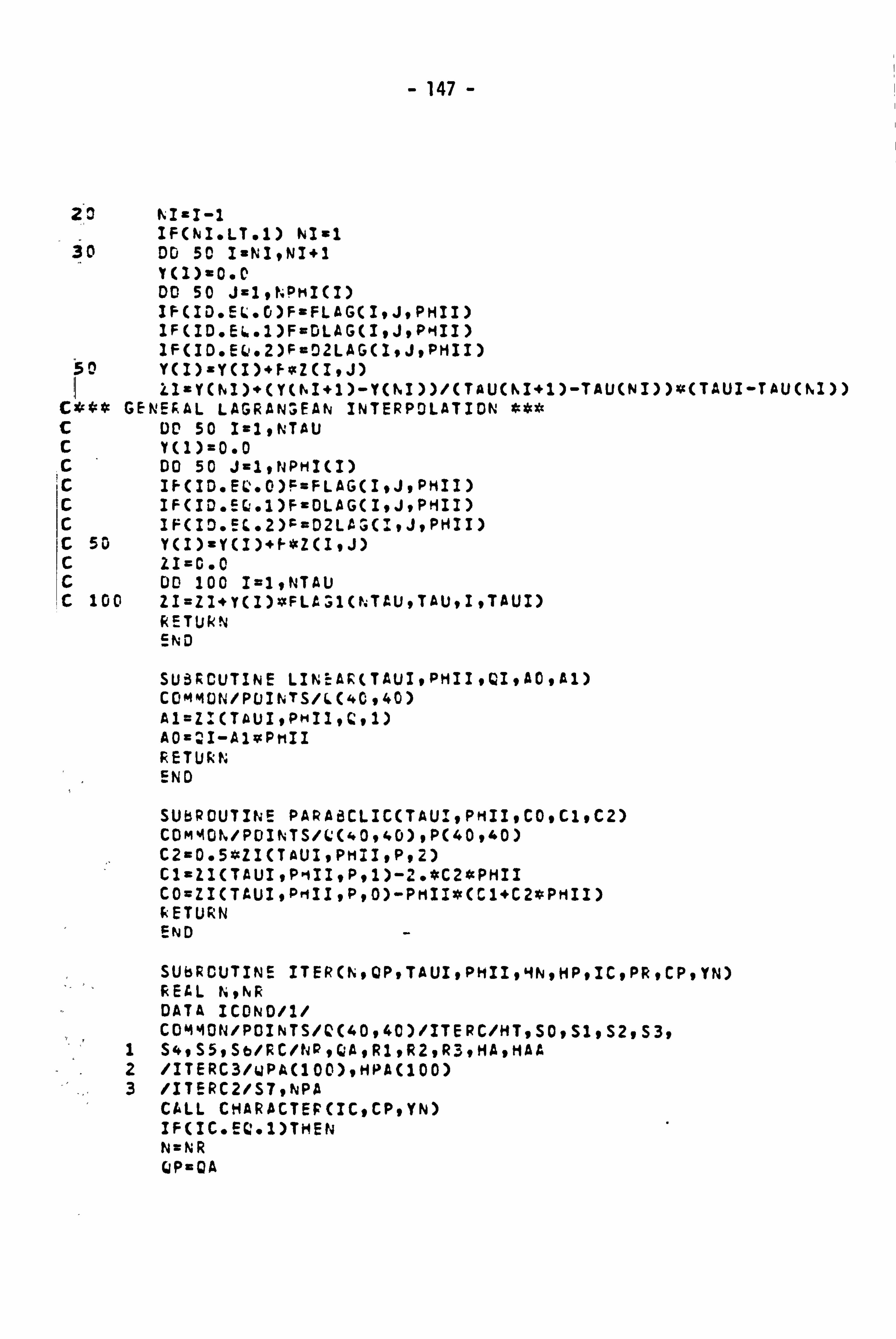
- 147 -

2110 NIZI-1 IF(NI*LT91) NIml

30 00 So IxNIqNI+l

Do 50 izigNPHI(l) IF(ID*EL*0)FzFLAG(I9J9PMII) IF(IO. E6. l)FwDLAG(IqJqPHII) IF(ID*EQ92)FuDZLAG(19JPPHII)

ýn. Y(I)SY(I)*Fqz(Itj) I llayCNI)*(Y(Nj+l)-YCNI))/(TAUCKI+1)-TAU(Nl))xc(TAUI-TAU(Nl))

C*** GFNEAAL LAGRANýEAN INTERPOLATION c DO 50 IvlqNTAU cy(1)z0.0 c DO 50 JzltNPHI(l)

ic IFCID*EQ. G)FxFLAG(ItJ9PHII) c IF(ID. EQ. l)FwDLAG(I9JqPHII) c IF(lO. EL*2)r-uD2LA%G(l9JvPHII) c so Y(I)zY(I)+ý*Z(IqJ) c 21=0.0 c DO 100 1=29NTAU c loo ZI=ZI+Y(I)VCFLAý1(t4TAUgTAU919TAUI)

(<ETUkN END

SUBROUTINE LINiAR(TAUIqPHIIqQIqA0qAl) COMMON/PUINTS/L(40940) Al=Z&'(TAUIqPHIlqQql) A0=21-Al*PmII RETUkN END

SUbPOUTINE PARA8CLIC(TAU&ljPHII9CO9Cl9C2) CDM40N/PDINTS/Q(40q40)qP(40q40) C2wOe5*ZI(TAUjqPHllqPq2) CIUZI(TAUIgPlilltPgl)-2. *C2*PHII CO=ZICTAU19PHIIgPvO)-PMII*(Cl+C2*PHII) IýETURN END

SUbRCUTINE ITER(N#QPPTAUItPH1194N*HPtICVPRtCPgYN) REAL NqNR DATA ICOND/l/ C044ON/PDINTS/C(40940)/ITEPC/HT9SO9Sl9S2gS39

I S49S59Sb/RC/NPtQAtRlPR29R39HAPHAA 2 /ITERC3/WPA(100)qHPACIOO) 3 /ITERC2/STgNPA

C4LL CHARACTEF(lCqCPqYN) IF(IC*EQel)TMEN NzNR QP=QA

- 148 -

HN a4A -0 .7 END IF Ir-(IC. EL. 2)THEN QP=QA tita(QP*(S2XtQP-1)+CP)/Sl-HT END IF IT=O

10 IT=IT+l SQHN=SQRT(4. N) PHIIzS3wN/SQHN IFUC. EL. I)RETURN IF(IC. GT. 2*At., D. IT*GT*5) THEN tiNz((CP-A3)/A2)**2 END IF PHIlaS3*N/SQgT(HN) Q&aZl(TAUIqPHIIqQq0) CALL LINEAR(TAUIqPH: IqQIqA0qAI) A2aAOý: Rl A3zAlmN*SS A4=S2-SI/42/A2 AS=2*; tSI3; cA3/A2/A2-1. AbaCP-Slu(MT+CA3/A2)**2) DDzA5*AS-4. *A4*A6 1F(A4. EL7.0.0)GO TO 200 IF(DDeLT*O. D)GO TO 200 DCPw((-A5-SQPT(OD))/A4/2. -QP) &., Pzwp+DIWP IF(ABS(DQP), LEo0,0C% '11)GO TO 30 IF(IT*GE. 2C)G0 TC 20 GC TO 10 PPINT%cq'xc*%cDIVEPGENCE' WRITE(2950)'AOtAl9A29A39A4tA59A69DQPPQP='t

1 A0#Aj9A2qA3jA4qA5qA5q9QPqCP STOP

30 HN2((QP-A3)/A2)*vcZ HP=HN+HT-S6*QP*QP Pgx, IP-HAA QPA(NPA+J)ZQP tiPA(NPA+l)z4P RETURN

20D, WRITc. (2950)'AC9AltA29A39A49A5, A6,00P, QPz', 1 AO9AltA29A39A49A59A690QPtQP

STOP'ITERATION EPROR' so FORMATCA30/9G12.4/)

END

SUBRCUTINE RUNGF(PHIIqTAUlqHN) DIMENSION ICOND(6) REAL KoKMtNRSFtKPoMCtNltN29N3tN49NCtKD DATA ICOND/6*1/

- 149 -

COMMON/INITIALC/YREF(6)qSEGMA CCMMON/PC/NRtQA9R29R29R3/DEC/EOPEIRtKtKMtNREFoTDgTI

I 9TAgKPgMCgNCgKD/RUNGEC/NT2MEgDTgY(6)gDY(6) c ** 9: * *** **** ******** 3k*** * **** *** * *** **** **** * ******* ** *)X

ONCY)=CEl/Y+E2*E3*Y)Y, &DT OG(VA9%^P)-CNC*VA*(YREF(3)/YREF(b))-G)/MC*DT OZ(DYgDGT)zKM/YPEF(5)*(K*DY+SEG4A*DGT*YREF(S))*NREF 02VO(DZT90VDgVD)=(KD*DZTvt(YREF(5)/YREF(4))-2*OVTDvDVD-VD)/

TD**2#OT2 D2VI(DVITgVIgZ)=(Zvc(YREF(c, )/YREF(2))-VI-2*TI*DVIT)

1 /TI**2*DTZ 02VA(VAqVIoVOgZtDVA)=(Vl*(Y'KEF(2)/YREF(3))+VD*(YREF(4)

1 /YREF(3))+KP9(Z*(YRc-F(S)/YREF(3))-VA-2*TArxDVA)/TA**2*DT2

12 Z F( Y9")g%M / yp E F'CD)*(K*Y+SEGMA*G*YREF(6»*NREF CALL PARABr-iLIC(TAUI9PHII9ColCI9C2) A7mRi*C 0 xcmKxcftl .5 AS=ý2*ClxcHN 492R3*C2*SI,. PTCHN) El zE 099A7-E 1R E2m =O rx AE E3ZEC*Ag DT2=DT*DT/2.

C X. c g; C; C. 7 * N:; c ig N1Zy(1) DN1mDNC>: 1) GIBY(6) VA1cYC3) DGIMDGCVAIPGJ) DZ1wDZ(DNIPDGI) DVDI=DY(4) VOlzYC4) D2VD1mD2vD(Dz190VD19VD1) DvIl=DY(2) VIlmy(2) 02vIlsD2V1CDVIlpvIlvDzi) 11Z1FCN1VG1) OVA1wDY(3) 02VA1z02VA(VAJ9VI19VD19Z1iDVAI)

C**e* ** * *Xt* * *** **3. N2r-YCI)+DNI/2 ÜNZMDN(N2) G2=Y(6)+DGI/2 VA2*Y(3)+DY(3)/2+D2VA1/4 0G2=DGCVA29G2) 0Z2=D&'. CDN2P0G2) DVD2=DY(4)+D2VD1 VO2mY(4)+DY(4)/2+D2VDI/4 D2V02uD2VD(DZ2P0V029VD2) DV12=DY(2)+D2VI1

- 150 -

Vl2zY(2)+DY(2)/2+DZVIl/4 D2Vld2-=D2VI(DVI29VI29DZ2) Z2zZF(h29G29) DVA2cDY(3)+D2VAl 0ZVA2cDZVA(VA29VIZ9VD2qZ2vDVA2)

t. 3=Y (i )+DNd'/Z UN3zDN(N3) G3aY(o)+DG2/2 VA3zY(3)+DY(3)/2+D2VAl/4 DG3=DG(VA39G3) D! 3=DZ(DNZtDG? ) OVD3=DY(4)+D2VO2 VD3=Y(4)+DY(I*)/Z+DZV01/4 02VD3=02VDCDZ39DVD39VD3) DV13zDY(2)+D2VI2 V13zY(2)+DY(2)/2+D2VII/4 02Vl3zD2VI(DV139VI39DZ3) Z3zZPCN39G3) DVA3zDY(3)+DZVA2 01'6VA3=02VA(VA39VI39VD39Z39DVA3)

C99 Vc OVC**

K4=Y(I)+D%? DN4=DN(N4) G4=Y(6)+DG3 VA4=Y(3)+DY(3)*D2VA3 DG4=DG(VA4 9 GO DZ4zDZ(ON49DG4) DV04=DY(4)+2*02VD3 VD4cY(4)+DY(4)+02VD3 D2VO4=02VD(OZ4qDVD4vVD4) DV14=DY(2)+2*02VI3 V! 4zY(2)+DY(2)+02VI3 D2Vl4=D2VI(OVj4qVI4vDZ4) 14=lF(N4qG4) DVA4=DY(3)+2*D2VA3 D2VA4zD2VA(VA4jVj4qVD4qZ4qDVA4)

C *)ý* *

Y(l)zY(I)+(DNI+23ccDN2+2*DN3+DN4)/6*0.92 Y(O)=Y(6)+(DGI+2*DG2+2*DG3+DG4)/6 Y(S)z&'F(Y(I)tY(6))*KP Y(4)=Y(4)+(02VD1+D2VD2+D2VD3)/3 UY(4)=DY(4)+CD2VDI+2vD2VD2+2*D2VD3+D2VD4)/3 Y(2)=YC2)+(D2VII+D2VI2+02VI3)/3 DY(2)=DY(2)+(D2VI1+2*02VI2+2*D2VI3+D2V4)/3 Y(3)=Y(3)+(D2VA1+D2VA2+02VA3)/3 DYC3)=DYC3)+CD2VA1+2*D2VA2+2*D2VA3+D2VA4)/3 IFCY(I)oLY. O. 99999999) NREF-lo IF(Y(I)eGT*1.0CD000j) NREFzl. kETURN

- 151 -

END

SUBROUTINE CHARACTERCICtCP) D416MENSION 00CO)PH(100) COMMON /ITERC/HTtSOlSJ/RC/NPtQA9Rl9R29R39HA/ITERC2/S79

I NPAtAREAtAtCtHS/ITERC3/QPA(100)PHPA(100) Cý*** COMPUTE STEADY-STATE CONDITIONS

IF( IC*Eý*2 )TtIEN FR cS 7gcL- A 3v*2 00 100 I=19NPA+l Q(I)zQA M(I)zHA-(I-l)*FP

100 CON TI NU E RETUkN END IF

ýc4c*vc INITILIZATI'6, N 1F(IC*9T. 2)TfiEN DO 150 1=29NPA+2 Q(l)zQPA(l) H(I)CHPA(l)

I *ý 0 CONTINUE END IF

CV*4 COMPUTE H AND C AT THE INTEPIOR NCDES DO 201 I=2, NPA Cpxg(j-l)+Slwm(1-1)-SD*QCI-1)*ABS(CCI-1))

UPA(I)x0o5*(CP+CN) tlPAcI)mo*5*cCP-CN)/Sl

201 CONTINUE C**4c '%. CMPJTE CP AT A DISTANCE OX FýOM THE INLET C, OF THE TURBINE

CP=I"kl(t. PA)+SlgtH(KPA)-SO*Q(N, PA)*ABS(QCNPA)) C*; C* CCMPJTE H AND Q AT UPSTREAM END ***

CN=L(Z)-SlvH(2)-SD3xQ(2)*ABS(Q(2)) G=(20.3*Sl)**2 9z40.6vcSl Fn-(C%+96oC*Sl) V=2*F E=l. C+R*F+20*3/85.0 H5zF*F-95.0/8590 17=0 IF(YN. EQ. 0.0) YN=1*3549

19 iTurT+l PYNmYN FlcS*PYN**4+R*PYN; t*3+E*PYN*#Z*V*PYN+Hb F2=4**-j*PYN**3+3**P*PYN**2+29*E*PYN+V DELYN=FI/FZ IF(ABS(DELYN), GT, DoCO1)DELYN=SIGN(O. 0019DELYN) YN=PYN-DELYN

- 152 -

21

31

IF(ASSCYN-PYN, ). LE. 0.0001)GO TO 31 IF(IT. GE. 20)GO TO 21 GO TC 29 PcINT*9'; c**DIVERGENCEP STUP MPA(l)z9b. 0-20.34cYN*YN QPACI)aCN+SlvcHOACl) RETURN END

- 153 -

I.

2.

REFERENCES

JAEGER, C. "Engineering Fluid Mechanics". Blackie and Son Ltd. 9 London. 1960.

SWIECICKI, I. "'Regulation of a hydraulic turbine calculated by step-by-step method". Journal of Basic Engineering, September, 1961/445.

PERKINS, F. E. "Hydropower plant transients" TEDROW, A. C. Dept. of Civil Engineering, Hydrodynamics EAGLESON, P. W. Lab., Report No. 71, Part II-III. IPPEN, A. T. Massachusetts Institute of Technology,

September, 1964.

WOZNIAK, L. "Conduit representation in closed loop FETT, G. H. simulation of hydroelectric system".

Journal of Basic Engineering, American Society of Mechanical Engineers, pp. 599-604, September, 1972.

WYLIE, E. B. "Fluid Transients". STREETER, V. L. McGraw-Hill Inc., New York, 1978.

CHAUDHRY, M. H. "Applied Hydraulic Transients". Van Nostrand Reinhold Ltd., Canada, 1977.

CHAUDHRY, M. H. "A non linear mathematical model for analysis of transients caused by a governed Francis turbine". 3rd International Conference on Pressure Surge, Canterbury, England, (Published by BHRA), March 25-27,1980.

"A palimpsest on the electronic analogue act". A. Philbrick Researches Inc., Massachusetts, 1955.

8. PAYNTER, H. M.

9. HOVEY, H. M.

10. CHAUDHRY. M. H.

11.

"Optimum adjustment of governors in Hydro generating stations". Engineering Journal, Engineering Inst. of Canada, pp. 64-71, November, 1960.

"Governing stability of a hydroelectric power plant". Water power, London, pp. 131-136, April, 1970.

THORNE, D. H. "Extension of stability boundaries of HILLs E. F. hydraulic turbine generating unit".

Trans. on Power Apparatus and systems, American Inst. of Electrical and Electronic Engineers, Aps. 94, No. 4, pp. 1401-1409. July/August, 1975.

- 154 -

12. DHALIWAL, N. S. "Analysis of PID governors in Multimachine WICHERT, H. E. system".

IEEE Trans. Vol. PAS-77, March/April, pp. 456-463,1978.

13. HAGIHORA, S. "Stability of hydraulic turbine generating YOKOTA, H. unit controlled by PID Governor". GODA, K. IEE Trans. Vol. PAS-98, No. 6, pp. 2294-2298, ISOBE, K. November/December, 1979.

14. PHI, D. T. "Analysis and application of the stability BOURQUE, E. T. limits of hydro-generating unit". THORNE, D. H. IEEE PES Winter meeting, Atlanta, Georgia, HILL, E. F. February, 1-6,1981.

15. COLLATZ, L. "The numerical treatment of differential equations". 3rd Edition, New York, 1966.

16. DELGADO, N. A. "Mathematical model of a stepping motor". Trans. IEEE, Vol. AC14, August, 1969.

17. PRENTER, P. M. IISýlines and variational methods". Jo n Wiley and Sons, New York, 1975.

18. ODEN, J. T. "An introduction to the mathematical theory REDDY, J. N. of finite elements".

John Wiley and Sons, 1976.

19. WOZNIAK, L. "Representation of pump-turbine character- FEFF, G. H. istics".

ASME paper No. 69-FE-7, June 16,1969.

20. BRITISH STANDARD 1042 "Methods of measurement of fluid flow in closed conduits". Part 1. Pressure differential devices, Section 1.1, BSI, London, 1981.

21. JONES, E. B. "Instrumentation, Measurement and feedback". McGraw-Hill, London. 1977.

22. JONES, M. H. "A practical introduction to electronic circuits". Cambridge University Press, London, 1982.

23. CLAYTON, G. B. "Experiments with operational amplifiers; learning by doing". MacMillan Press Ltd., 1978.

24. DOEBELIN, E. O. "Dynamic analysis and feedback control". McGraw-Hill, London, 1962.

25. RAVEN, F. H. "Automatic control engineering". McGraw-Hill Kogakusha Ltd. London. 1978.

- 155 -

26. BENEDICT, R. P. "Fundamentals of temperature, pressure - and flow measure'ments". John Wiley and Sons, London, 1976.

27. KRUGER, R. E. "Selecting hydraulic reaction turbiTtel'. Engineering Monograph No. 20, United States Department of the Interior, Bureau of Reclamation. 1980.

j. m. hassan - core · 2013-06-04 · cranfield institute of technology department of fluid...

Documents