j: copy

GL-TR-90-0093

AN ASSESSMENT OF THE APPLICATION OF IN SITU ION-DENSITY DATAFROM DMSP TO MODELING OF TRANSIONOSPHEI:IC SCINTILLATION

NDTy James A. Secan

y Lee A. Reinleitner ELECTERobert M. BusseyNorthwest Research Associates, Inc. JUL 3 0 1990P.O. Box 3027

Bellevue, Washington 98009 0 'J '

15 March 1990

Final Report15 September 1989 - 14 March 1990

Approved for public release; distribution unlimited

Prepared for:

GEOPHYSICS LABORATORYAIR FORCE SYSTEMS COMMANDUNITED STATES AIR FORCEHANSCOM AFB, MASSACHUSETIS 01731-5000

"This technical report has been reviewed and is approved for publication"

/Z/.f/

EDWARD J. WEB&f VICKERYContract Manager/Branch Chief

FOR THE COMMANDER

ROBERT A. 4RIVANEKDivision Director

This report has been reviewed by the ESD Public Affairs Office (PA) and isreleasable to the National Technical Information Service (NTIS).

Qualified requestors may obtain additional copies from Defense TechnicalInformation Center. All others should apply to the National TechnicalInformation Service.

If your address han changed, or if you wish to be removed from the mailinglist, or if the addressee is no longer employed by your organization, pleasnotify GL/IMA Hanscom AFB, MA 01731. This will assist us in maintaining acurrent mailing list.

Do not return copies of this report unless contractual obligations or noticon j specific document requires that it be returned.

WSUIT CLASSIFICATION OFTHIS PAGr

REPORT DOCUMENTATION PAGEIa. REPORT SECURITY CLASSIFICATION lb. RESTRICTIVE MARKINGS

Unclassified__________________________2a SECURITY CLASSIFICATION AUTH-ORITY 3. DISTRIBUTION/ AVAILABILITY OF REPORT

Approved for public release.2b. DE CLASSIFICATION I DOWNGRADING SCHEDULE Distribution unlimited.

4. PERFOAMING ORGANIZATION REPORT NUMBER(S) S. MONITORING ORGANIZATION REPORT NUMBER(S)

NWRA-CR-90-R060 ;-1-.oo96a. NAME OF PERFORMING ORGAN:ZATION 16b. OFFICE SYMBOL 7a. NAME OF MONITORING ORGANIZATION

* (if applicable)Northwest Research Assoc. Inc CR Geophysics Laboratory6c. ADDRESS (City, State, and ZIP Codfe) 7b. ADDRESS (City, State, and ZIP Code)P.O. Box 3027 Hanscom AFB3, MA 01731-5000Bellevue, WA 98009

Ba. NAME OF FUNDING ISPO;.SORING 8b. OFFICE SYMBOL 9. PROCUREMENT INSTRUMENT IDENTIFICATION NUMBERORGANIZATION 1 (if applicable)

I ________ 19628-86-C-01958c, ADDRESS (City, State, and ZIP Code) 10. SOURCE OF FUNDING NUMBERS

PROGRAM PROJECT TASK WORK UNITELEMENT NO, NO. NO, ACCESSION NO,62101F 4643 I 09 Al

11. TITLE (include Security Classification)An Assessment of the Application of in situ Ion-density data from DMSP to modeling ofTransionospheric Scintillation12. PERSONAL AUTHOR(S)Secan. Jamres A. . Lee A. Reinleitner, Robert M. Bussey13a, TYPE OF REPORT 13b, TIME COVERED 114. DATE OF REPORT (Yeair, Mnth, ay 15. PAGE COUNTF~inal Report TFROMJ9'_1J TO,2 4 4 199 ac 15 3216. SUPPLEMENTARY NOTATION

17. COSATI CODES 18. SUBJECT TERMS (Continue on reverse if necessaryl and Identify by block number)FIELD GROUP "2 I :.>Ionospheres Tonospheric Scintillation, iuioiowave Scintil.--

20 14 I aion,_.P. efense Meteorology Satellite Program (DMS1')1197% ýSARCT (Continue on reverse if necetsary and identify by blockfi~mboi..r). / i I. 7 (

-L-'Modemn military coinmmunication, navigation, and surveillance systems de~pend on reliable, noise-frce transionosphcric radio-frequency channels. They can be severely impacted by small-scale electron-density irregularities In the ionosphere, which cause bothphase and ampliur~ide scinltillationI BaIsic tools used in planning anti mitigation schemcs arc, climatological in nature and thus maILygretitly over. and under-estimate thec ffects of' scintillalion in a given scenario. This report summarizes the results of a tlirce-yearinvestigation into thc feasibility of using in-situ observations of thc ionosphcre rrom the USAF DMSP satellite to calculate estimatesof irregularity parameters that could be used to update scintillation modols in near real-time, Estimates for the level or intensity andphase scintillation on a transionospheric UHIF radtio link In the early-evening auroral zone were calculated fromt DMSIP ScintillationMeter (SM) data and compared to the levels actually observed. 'The intensity scintillation levels predicted and observed comparedqluite well, but the comparison with the phatse scintillation data was complicated by low-frequency pha~se noise oti the 111WF radio link,

* Results are presented from analysis of1 DMVSP SSIES date collected near Kwajalein Island in conjunction with a propagation-el'kctsexperiment, Preliminary conclusions to the assessment study are (1) the DMSP SM data can be used to make quantitaive estimalttes ofthe level of'scintillation at auroral lutitudes, and (2) it may be possible to use the data a% a qualitative indicator of'scintillation-activity

* levels at equatorial latitudes, .. ((,. '

20. DISTRIBUTION /AVAILABILITY OF ABSTRACT 21. ABSTRACT SECURITY CLASSIFICATIONOUNCLASSIFIEci/UNLIMITEO 0J SAME AS RPT. ODTIC USERS Un' ufied

22s. NAME OF RESPONSIBLE INDIVIDUAL 22b TELEPHONE (include Area Code) 22c. OFFICE SYMBOLEdward WeberI L'lI

DD FORM 1473, 84 MAR 83 APR edition may be used until exhausted, SECUR~ITY CLASSIFICATION OF, Hl$ PAgEAll other editions are obsolete.

Unci I ss i f led

a

a

ii

TABLE OF CONTENTS

PAU

1. Introduction . . . . . . . . . . . . . . . . . . . . . . . . . . . . . . . . . . . . . . . . . . . . . . . I

2, B ackground . . . . . . . . . . . . . . . . . . . . . . . . . . . . . . . . . . . . . . . . . . . . . . .2

3. Analysis of SSIEPS/AIO/EISCAT Campaign Data ........................ 5

4. Sum m ary of Project Results ..................................... 10

4.1 Study of Methods for Calculation of Ck ......................... 10

4.1.1 Procedures for Calculating CkL ......................... 10

4.1.2 Uncertainties in CkL ............................... 124.2 Auroral Region Studies ..................... ... ... ...... . 144,3 Equatorial Region Studies ................................... 17

5. C o nclusion . . . . . . . . . . . . . . . . . . . . . . . . . . . . . . . . . . . . . . . . . . . . . . .2 1

R eferences . . . . . . . . . . . . . . . . . . . . . . . . . . . . . . . . . . . . . . . . . . . . . . .23

Appendix, Topside Electron Density Model .............. ............. 25

(. I' 1A It I,. ,L .'' d [-

1).,tA ll' . .

iii

LIST OF FIGURES

Figure Caption Page

I Total ion density data from the SSIES Scintillation Meter (SSIES/SM) (a) 6and the corresponding electron density profiles generated from theSSIES/SM data for the 8 January 1988 pass. The x-axis labels in (a) arefor the satellite location, those in (b) are for the 300-km field-line"footprint." The x-axis labels are GLAT for geographic latitude, GLON forgeographic longitude, ALT for satellite altitude, APXLAT for modifiedapex latitude, APXLON for apex longitude, and APXLT for ipex localtime.

2 Data from Figure l(a) replotted to the "window" sampled by the EISCAT 8radar. Note the reversal of north and south from Figure 1 (a) to this figure.

3 Data from the 8 January 1988 campaign day: (a) detrended intensity data 16from the A10-AFSAT VHF radio link, (b) detrended phase data from thislink, and (c) total ion density from the SSIES/SM sensor. The plots arealigned to cover roughly the same spatial region.

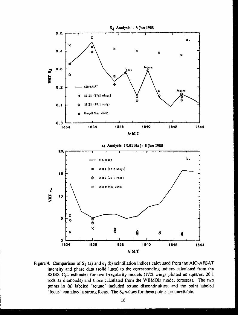
4 Comparison of S4 (a) and a, (b) scintillation indices calculated from the 18AIO-AFSAT intensity and phase data (solid lines) to the correspondingindices calculated from the SSIES CkL estimates for two irregularitymodels (17:2 wings plotted as squares, 20:1 rods as diamonds) and thosecalculated from the WBMOD model (crosses). The two points in (a)labeled "retune" included retune discontinuities, and the point labeled"focus" contained a strong focus. The S4 values for these points are unre-liable.

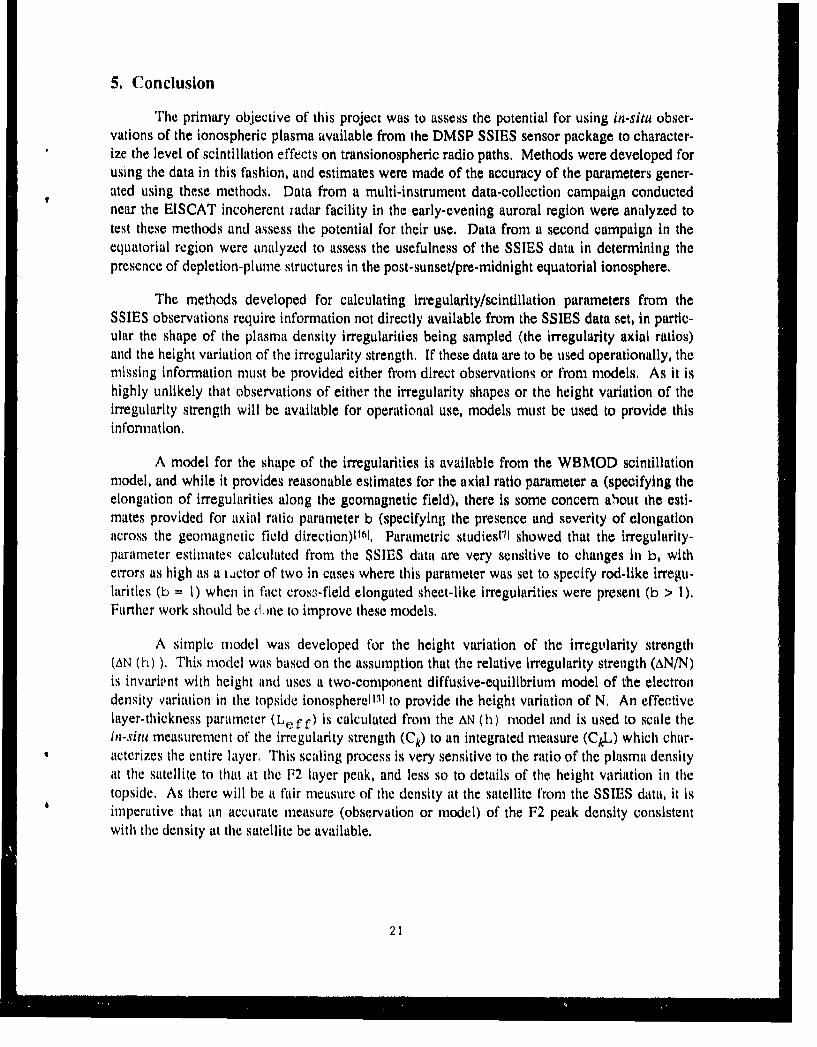
5 Total ion density measured by the SSIES/SM sensor on DMSP F8 near 20Kwajalein on 24 August 1988, The y-axis is ion density, ranging from 0,0to 2,0xi05; and the x-axis labels are GMT for Greenwich Mean Time(1-HIl:MM:SS), ArX'×,AT for mdlified apex latitude, and ^ Xl ,U.N for apexlongitude.

iv

LIST OF TABLES

Table Caption Page

I Parameters for the electron density profiles plotted in Figure 2. 9

V

PREFACE

This report summarizes the work completed during an investigation into the feasibility ofusing in-situ observations of the ionosphere from the DMSP SSIES sensors to calculate parame-ters that characterize ionospheric scintillation effects, This work is part of a larger effort with anoverall objective of providing the USAF Air Weather Service with the capability of observingionospheric scintillations, and the plasma density irregularities that cause the scintillations, innear real-time and updating models of ionospheric scintillation with these observations,

vi

I. Introduction

Many modern military systems used for communications, command aid control, naviga-tion, and surveillance depend on reliable and relatively noise-free transmission of radiowavesignals through the earth's ionosphere. Small-scale irregularities in the ionospheric density cancause severe distortion, known as radiowave scintillation, of both the amplitude and phase ofthese signals, A basic tool used in estimating these effects on systems is a computer program,WBMOD, based on a single-scatter phase-screen propagation model and a number of empiricalmodels of the global morphology of ionospheric density irregularities[1 .21. An inherent weaknessof WBMOD is that the irregularity models provide median estimates for parameters with largedynamic ranges, which can lead to large under- and over-estimation of the effects of the iono-spheric irregularities on a system.

One solution to this problem, tit least for near real-time estimates, is to update theWBMOD irregularity models with observations of the various parameters modeled. Oneproposed source for these observations is from the in-situ plasma density monitor to be flown onthe Defense Meteorology Satellite Program (DMSP) satellites. Previous studiesl31 using in-situmeasurements from the DE-2 satellite have found that there is potential for using the data in thisfashion. This study is designed to assess the applicability of this data set to real-time updates ofthe WBMOD models, There are two primary objectives:

(1) Develop and refine techniques for generating estimates of parameters that char-acterize ionospheric scintillation from in-situ observations of the ionospheric plasma from theDMSP SSIES sensors.

(2) Determine if the parameters calculated from the SSIES data can be used tocompute the scintillation effects on a transionospheric radiowave signal.

This report describes one final aspect of the analysis of data from a campaign conductednear Tromso in January 1988 and summarizes the findings and results of the entire project,

2. Background

The propagation model used in the WBMOD program (based on weak-scatter phase-screen theoryll.2)) characterizes the ionospheric electron density irregularities that cause SCin-tillation via eight independent parametersl 4l:

(1) a: The irregularity axial ratio along the direction of the ambient geomagnetic field,

(2) b: The irregularity axial ratio perpendicular to the direction of the ambient geomagneticfield.

(3) 8: The angle between sheet-like irregularity structures and geomagnetic L shells.

(4) h,: The height of the equivalent phase screen above the earth's surface.

(5) Y: The in-situ irregularity drift velocity,

(6) ao: The outer scale of the irregularity spectrum.

(7) q: The slope of a power-law distribution that describes the one-dimensional power-density spectrum (PDS) of the irregularities.

(8) CkL: The height-integrated strength parameter.The first three parameters (a, b, and 8) and the direction of the ambient geomagnetic field specifythe propagation geometry, while the last three (ao, q, and CkL) specify the spectral characteris-tics of the irregularities.

It may be possible to obtain estimates for the values of three of these parameters from theDMSP SSIES sensors: Yd (from the SSIES Ion Drift Meter (DM)), and q and CAL (from theSSIES Ion Scintillation Meter (SM)). In this study, we will focus on the estimation of CkL fromthis data set and consider q and yd only in terms of the effects of uncertainties in these parame-ters on the estimates of CkL. Of the eight parameters, CkL varies the most as a function of loca-tion and time, and has the most profound effect on the accuracy of estimates of scintillationlevels made by the WBMOD model.

In the phase-screen propagation theory used in WB3MODI 41, the Ckl, parameter is actuallythe product of two parameters: Ck , the three-dimensional spectral "strength" of the electrondensity irregularities at a scale size of I km* (related to the structure constant used in classicalturbulence theory); and L, the thickness of the irregularity layer. The models in WBMOD wereobtained from analysis of phase scintillation data from the WIDE1BAND and HiLat satellites,which will provide estimates of the height-integrated value of CkL rather than independent

* The cited reference develops the theory in terms of an earlier definition of the strength param-

eter, C ,, which is defined at a scale size of 2n meters. It is related to Ck according to the equa-tion CS = (2x/l(XX))q+ 2 Ck.

2

measures of Ck anid l. Because of this, the model was developed for Ckl. rather than for (Ck andL separately.

The calculation of an estimate of the CkI, parameter from topside in-situ ion densityobservations requires two operations. First, an estimate of Ck at the satellite altitude is madefrom a finite-length time series of density measurements. Second, the estimate of Ck isconverted to an estimate of CkL in some fashion which will account for both the thickness of theirregularity layer and the variation of Ck, or <AN, 2>, within the layer.

The data set from which the estimates of these parameters are to be obtained will becollected by three instruments in the DMSP SSIES (Special Sensor for Ions, Electrons, andScintillation) sensor package, This data set will contain the following in-situ observations:

(1) High time-resolution (24 samples/sec) measurements of the ion density andmeasurements of the ion density irregularity PDS at high fluctuation frequencies from the IonScintillation Meter (SM)[. 51,

(2) Measurements of the horizontal and vertical cross-track ion drift velocities from theIon Drift Meter (DM)I.I,

(3) Measurements of the ion and electron temperatures, the densities of 0+ and thedominant light ion (1l+ or He+), and the horizontal ram ion drift velocity from the ion RetardingPotential Analyzer (RPA)[61,

The basic data of this set are the high time-resolution density data from the SM which will beused to generate estimates of the irregularity PDS. The drift-velocity measurements from theDM and RPA will be used in calculating an estimate of Ck from parameters obtained from thePDS, and the other measurements from the RPA will be used in calculating CkL from Ck,

In the first year of this project, techniques for calculating estimates of CkL from theSSIES data set were developed, and parametric studies were conducted to determine the uncer-tainties in the final CkL estimates due to uncertainties in the parameters and procedures used tocalculate the estimates. Since the first SSIES sensor package was not flown until mid-1987,these studies were conducted using simulated SM density data sets and phase scintillation datafrom tile Wideband satellite, The results of these sttdies were reported in Scientific Report I forthis projectl'l (herein referred to as Repoit 1) and will be summarized in Section 4,1 of thisreport.

The second phase of the project, which focuses on how well these techniques work usingdata froml the DMSP F8 and `9 spacecraft, was begun during the second year of the project. Acoordinated, multi-sensor observation campaign was conducted during January 1988 in thevicinity of Tromso, Norway, in order to collect data for this study. The GL Airborne Iono-spheric Observatory (A10) aircraft flew repeated north-south legs along the magnetic meridian attimes when the DMSP F8 satellite was passing overhead. Data collected on the AIO included

3

intensity and phase scintillation observations on a VHF link from an AFSAT satellite, auroralimages from an all-sky photometer, and ionograms from a digisonde. Ionospheric soundings bythe EISCAT incoherent-scatter radar located in Norway also were made aperiodically throughoutthe observation period. Data were collected for DMSP passes on 8, 9, 15, 16, 17, and 18 January1988. The procedures used to process these data and results from the analysis were reported inScientific Reports 2 and 3 for this projectrR. 91 (herein referred to as Reports 2 and 3) and will besummarized in Section 4.2.

During the third year, a complete analysis was made SSIES data collected from bothDMSP F8 and F9 during a multi-sensor campaign conducted by the Defense Nuclear Agency(DNA) near Kwajalein Island were analyzed to determine the usefulness of these data for scin-tillation characterization in the equatorial ionosphere, The results of these studies werepresented in Report 3 and are summarized in Section 4.3 of this report.

A note on coordinate systems: The geomagnetic latitude, longitude, and local time coor-dinate system used throughout this report is modified apex coordinatesll01, a coordinate systemderived from apex coordinates proposed by VanZandt et all'tU. This system, which is used in theWBMOD model, was chosen because it is very similar to both invariant and correctedgeomagnetic coordinates at high latitudes, and modified apex latitude is very similar to dip lati-tude in the equatorial region, becoming identical to dip latitude at the dip equator.

3. Analysis of SSIES/AIO/EISCAT Campaign Data

In Report 3, the results from a detailed analysis of the data collected on 8 January 1988wc.re presented. One aspect of the data analysis which was not presented in detail was a discus-sion of the electron density profiles used to generate the effective layer thickness parameter,

Le f f, which is used in turn to calculate an estimnate of CkL from the Ck value derived from thein-situ Scintillation Meter (SM) ion density measurements. In this section we will describe theway in which these profiles were generated and present examples of the profiles used in the 8January analysis.

The model used to generate the profiles is a two-component diffusive-equilibrium modeldeveloped several years ago for building profiles from SSIES obseivations (see Appendix).Inputs to the model include the critical frequency of the F2 peak and the height of the peak (foF2and 1 rmF2 ), the semi-thickness c..' the topside just above the F2 peak, the electron density (or totalion density) at some height in the topside, and either the height at which the 0+ and H+ numberdensities are equal (i.e., the O+/H+ transition height) or the ratio of 0+ to H+ at some height inthe topside, In addition, the model has several "free" parameters which can be adjusted tochange the shape of the profile. Any of the input parameters can be adjusted within the model tofit the profile to the other inputs, For example, in the present study the foF2 and hmF 2 valueswere adjusted to fit the profile to the total ion density observed by the SM sensor,

The procedures to build the profile used to calculate Leff were as follows:

(1) Calculate the avenage total ion density for the data set used to calculate Ckfrom the density-trend time series removed from the SM density measure-ments in the detrending process.

(2) Trace down the field line passing through the center of the data sample to analtitude of 300 kil.

(3) Calculate estimates of foF2 and h1.F2 using the CCIR coefficients for foF2and M3000 and values for the O+/H+ transition height and the topside semi-thickness at this location.

(4) Iteratively adjust the f0F2 and hmF2 parameters to fit the profile to the aver-age density calculated in step (1),

'T'his profile arid a model for the height variation of the irregularity strength as a function of thebackground plasma density are then used to calculaite 'e f,

Figure 1 shows the SM density record from the 8 January 1988 pass near Tromso (upperplot) and a contour plot of tile corresponding electron density profiles which were generated tocalculate Le f f. The locations and geomagnetic local time (APXLT) along the x-axis of the in-situ density plot are calculated at tile satellite altitude, and those along the x-axis of the profileplot are calculated at the 300kmi "footprint" of the field line passing through the satellite location.

5

1.5- .

-0 1.0 I

I(

0 a .L

UT sc 1c 66990 67030 67110 67170 67230 67290 Utl5EC)SLAT 77.91 75,27 72.32 6T. 19 65.9 U62. 63 CLAYiLQN @40:,04 29,9 12: 51 17.0 13. 312 10. 07 QLOH

ALT 657 56 657,N 859 1 2 958 0.29 659 39 56 *41 ALTAF'XLAT 73 93 71.21 70 03 67.44 64. 59 63. 5: APXXLATAPXLON 1300.12 at 7,1 1 I:7107 10OM6 97,05 90.06 AP LONAPXLT 22.4608 R11.1 21.13 01 0.653 20.493 20,112l APXLT

9. 00 - - '

200 1:::,, ____________

100

S oAT ...4....73 1 7.16 .093.. 94 SLA

SLN40 .900 22 31.03.I .0OO

0~ bCLA 3..6 75.98 WJE.h1 IIIIE1IJL. 9 439 CA

OLON ~ ~ ~ ~ LG( 6 (cm3 )2.4 11 1.1 9"CO

GPLON for gegapi logtue ALT.6 for saelit alitde 43A for9 m XOdiidaelAtie XL XLT fo 1pe logtue0ad.X orae lcl7ie

22.03 1962 2 20i3 0.6 A 6

The slight tilt to the right in the profile plot is due to mapping the profiles constructed along fieldlines, I Notc: The profile plot shows no ionization in the E region because the model used doesnot include an auroral precipitation-produced E region, and there is no solar component as the Eregion is dark throughout the pass. This (toes not affect the results, however, as the model usedto calculate Ckl, assumes that all contributions to the integrated irregularity strength come fromthe F2 region.)

Our initial hope was to use profiles from the EISCAT radart as part of the study, but therehave been difficulties in putting the radar data into useful forn. One figure showing a contourplot of electron density from a roughly north-south meridional scan from the radar with a centertime of 18:34:40 GMT (668(X) seconds past midnight) has been received for comparison with theprofiles used in the Leff calculation, Unfortunately, this figure is in color and could not belegibly reproduced in black and white for this document.

We have, however, replotted a subset of the model profiles in the same format as thecolor figure showing what the radar would have seen if it had sampled our model ionosphere(Figure 2), This figure has the same contour levels as in Figure 1, but the x-axis has beenreversed (north is nov to the right) and is plotted in the corrected geomagnetic (CG) latitude ofthe 3(X) km "footprint" location. The irregular shape of the sampled region corresponds to thatshown in the color plot provided of the EISCAT data, The model parameters used to build theseprofiles and the resulting Lef f values are listed in Table 1.

Quantitatively, the radar data and model "prediction" agree fairly well. Both show an F2-region enhancement at the northern edge of the sampled region, a lesser enhancement at thesouthern edge, a "tongue" of enhanced density reaching from the northern enhancement to thecenter of the sampled region, and a region of low plasma in the topside between CG latitude65,50 and 680, There are some discrepancies in details, The altitudes of the peak in the modelprofiles average about 30-50 km above the estimated peaks in the radar data, and the enhance-ment at the northern end of the region is further from Tromso in the radar data than is shown inthe rnodel profiles, Unfortunately, no quantitative comparison of the density levels was possibleas the color plot of the radar data was of relative rather than absolute density.

7

LOG (N0 ) (cm-

3.6 40 4.4 4.8 5.2

800 L W.I

700

600

.~ .....

300

100

64 65 66 67 68 69 70 71 72

Corrected Gconulnet ic L..nt itUde

Figure 2. Data from Figure I1(a) replotted to the "window" sampled by the EISCAT radar, Notethe reversal of north and South from Figure I (a) to this figure,

T' I M V . GI-AT C;11.N ( IAT CCI.ON Vo"VPv. fuG- hm.i'2 -. hml.'" Yt Itl I I, .I t

6'*055 15. 76 29.39 11 .61 118,88 2.85 3.8"1 32'.95 344.11 84,2"14 1195.13 3 3.151E#0767060 15.53 28,68 11.43 118.10 2.82 3,68 321.62 342.00 83.887 119S.13 3 3.266E",€0767065 15.70 2,.99 11,26 117,32 2.80 3,64 327.28 341.35 83.508 1195.13 3 3.2111-.'107671010 15.01 21,33 '1 .0l 116,56 2.'17 3,64 326.95 341.13 83.14? 119S.13 3 3. 210P.4 OI67015 14.84 26.68 "10.90 115,81 2.75 3.52 326,61 339.37 82.186 1195.13 3 3.3621+01'61080 74.61 26,05 70.72 115.06 2.73 3,27 326.27 335.44 82.440 1195.13 2 3.5491%40760085 74.31 25.44 70.53 114.31 2.10 2,97 325.93 330.61 82,105 1195.13 2 3.7971E+0167090 74.13 24,85 '10.33 113.57 2.68 2.85 325,59 328,58 81.779 1195.13 2 3.897E+0764095 13.90 24.21 710.15 112.88 2.66 3.03 325.25 331.50 81.463 1195.13 2 3.713E+0767100 73.66 23.70 69.96 112.20 2.64 3.38 324.90 336.70 81.158 1195.13 2 3.42411,40767105 73,42 23.16 69.76 111.54 2.61 3.69 324.55 339.86 80.861 1195.13 3 3.255t1+076•110 '13,1'1 22.63 69.55 110.88 2.59 3.81 324.21 340.60 80,5'15 1195.13 3 3,2071F.0761115 U.293 22.11 69,36 110,23 2.57 3,12 323.86 339.52 80.291 1195.13 3 3.24511.+0'67120 12.68 21,60 69,15 109,51 2.55 3.49 323.51 336.94 80.028 1195.13 3 3.355E101'67125 72.44 21,11 68.95 108.93 2.53 3.22 323,16 333.57 79,769 1195.13 2 3.51011#076*1130 '12 19 20.63 68.14 108.29 2.51 3,00 322.81 330.30 19.518 1195.13 2 3,666E+0761135 '1 ,94 20,1"1 68 5:3 1071,66 2.49 ,'19 322.45 327,06 '19.281 1195.13 2 3.829L1O*061140 11,69 19.711 68.31 107.08 2.48 250 322.10 322.49 19.064 1195.13 1 4.0791E40'161145 71.45 19,21 68.11 l06.b3 2.46 2.20 321.15 317.74 78,855 1195.13 2 4.3603E0'161150 ?1.19 18,83 6V.88 105,95 2.44 2.09 321.39 316.10 70,652 1195.13 2 4.,1491E#0767155 '0.94 18,41 67.61 105.3t 2.43 2.10 321.04 317.27 78,457 1195,13 2 4.354E140761160 '10.69 18.00 61.45 104.44 2.41 2.22 320.60 311.85 78.269 1195,13 2 4.300E1.0761165 '10,44 17.60 60.23 104.30 2.40 2,14 320.32 316.46 18,081 1195.13 2 4.3'13E+076/11'10 '10.18 17,20 61.00 103,14 2.38 2.01 319.91 314.44 71.913 1195.13 2 4.492E1.076711b 69.93 16.82 66,18 103.22 2.37 1.95 319.61 313.45 171,745 1195.13 2 4.5432.4076"1180 69.61 16.44 66.55 102,11 2.36 1.94 319.26 313.18 17,584 1195.13 2 4.54631.+0"671181 69.42 16.08 66.3:3 102.23 2.34 1,90 318.90 312.42 '17.430 1195.13 2 4.58413001601190 69.16 15,72 66.10 101, 74 2 33 1,19 318.54 310.8 U '17,211 1 95, 1 1 4.67-11.0U161195 6H.90 1., :3) 65 .81 1)1,.26 2. 32 1,66 :311,19 308,99 711. 142 1195,1:3 3 4. 110 1 El', 167200 68,65 1b.07 65h65 100, 19 2. 31 1.S0 31 1.83 307 16 *11.0 1) 119.5.13 3 4.11|101' 0f161205 68.39 14,69 65.41 100.31 2,30 1,64 3117,41 308.31 '16,881 1195.13 3 4.332531.0'61I10 68,13 14,36 65.19 99,84 2.29 1.0! 317.12 :10.088 16.7160 1195.12 2 4.62431,11'61215 67.81 14,04 64.94 99.38 2.29 2,08 316,16 313.84 16,646 1195.12 2 4.4110+0161220 61.61 13,12 64.70 98.94 2.20 2.21 316.11 315.49 16.530 1195.12 1 4.294tV0761225 6V,35 13.41 64.46 98.49 2.21 2,23 316,05 315.48 16,431 1195.18 1 4.286E1+0761230 61,09 13,11 64.21 98,06 2,21 2,20 315,10 314.75 76.342 1195.26 1 4.3241+01'61235 66.83 12.02 6:3,96 971,63 2.26 2,11 315.35 314,04 76.253 1195.31 1 4.362E+07

Loerind t

TIMF St..ondn ai nlc'. m idn.tqh.t (GMT)GLAT GnotrAphl " ];t. Iltuch.CG 1.0N I riph l C w I 'riI t.uw •CcIAT' Cr r roct.ud (?(i m.'.,tit ! c I at. I t ud.CIII.(N Cur rnot vd vtn•r• .jn.t I c I ontl I t utitf()V2I Iui t. taI] fol",' (IIum UC I I)I (I 2 fol+2 from pro i It, f I t. to in- l I t.u .rnityhml'"2, In It. l, I hml.'2 lt urm CCtI K)hml"2 l, 2 f rom prutio fII IlL Lo in-'slt.U dow-rityYL Topside Iayor thickrinas paramot.orlit (Of/It+ ' rainslt ion huljht.N Number of Lurit ltoti.I for proftl+ fitit t f " uft. Ivo Iyor t.hi uk tri, par.imoter (m)

N!)It. I IEc! i A cAt.wr; have beun traicord down th local f ' ldInrt .uo 300 rrm iI I Ltudo I

"rable I. Parameters for the electron density profiles plotted in Figure 2,

9

4. Summary of Project Results

4.1 Study or Methods for Calculation of (41C

The goal of this study was to develop a method for calculating an estimate of CkL fromdata collected by the SSIES plasma probes and to make a determination of the uncertainties inthese estimates.

4.1.1 Procedures for Calculating CkL

According to phase-screen theoryl2l, if the power-density spectrum (PDS) of the plasmadensity irregularities are assumed to follow a single-regime power-law model, an estimate for thespectral strength parameter, Ck, can be calculated from In-situ measurements of the plasmadensity irregularities from

103>-

Ck - 5.0x10 8 q [1]

where q and T1 are the slope and intercept of a log-linear fit to the PDS calculated from theplasma density data, and Vp is an effective velocity of the satellite with respect to the irregulari-ties. This last parameter is defined in a coordinate system defined by the geometry of the irreg-ularities and is given by

Vp VT C v (21

where v is the vector velocity of the satellite with respect to the irregularities (which includes thesatellite's orbital velocity and the in-situ velocity of the irregularities), and C is a transformattionmatrix derived from a generalized model of the irregularity geometryll21,

The procedure developed for calculating parameters q and T, from the SSIES Scintilla-tion Meter ion density data is as follows:

(1) I)eirend the ion density data by removing a background trend. This trend canbe calculated from either a low-pass filter applied to the entire data set or aquadratic least-squares fit to each data sample (256 or 512 points),

(., Apply a tirrc-domain window to the detrended data sample. The window ofchoice is a 30% split-bell cosine taper.

(3) Use ain FFl of the detrended, windowed data sample to calculate an estimiateof the P1)S (¢N).

10

II I II 1I I I IIII I I

(4) Smooth the PDS estimate, The smoothing function used is a five-point, cen-tered function with binomial weights.

(5) Use a linear least-squares fit to log(PDS) versus log(frequency) over the fre-quency range 0.3 to 5,0 Hz.

The various parameters in this method, such as the severity of the windowing function and thefrequency range for the PDS fit, were determined from a series of parametric studies usingsimulation data generated with known spectral characteristics (see Report 1) and were validatedagainst a sample of data from the SM sensor on DMSP satellite F8 (see Report 2),

The calculation of and estimate of Ckl. from an observation of Ck at the satellite altitude,<, is hased on the following assumptions:

(1) The altitude at which the Ck measurement is made is within the irregularitylayer,

(2) The measured Ck is representative of' conditions throughout the irregularitylayer,

(3) The geometry of the irregularities, and the slope of the irregularity PDS, arerelatively constant throughout the height range of the irregularity layer.

(4) The variation of Ck, or <AN 2 >, with altitude throughout the irregularity layeris known, or can be modeled,

These assumptions lead the following relationship between CkL and Ck:

(kL = Ck Lief [3)

where Le, f f is an effective layer thickness parameter, given by

fhs <AN2> dh

Lb (41< ':AN 2 >

where hb) is the height of the hottom of the irregularity layer and <'AN 2 >, is the density varianceat the satellite altitude,

For this project, we have chosen a ."imple model for the variation of <AN 2 > with altitudewhich assumes that the layer extends from 1/4 of a scale height below the P2-layer peak height

11

to the satellite altitude, and that the ratio of <AN 2 > to the background density is constant

throughout the layer. This changes Equation [41 to

fhs Ne 2 (h) dh

hbLeff - [5]

Ne2 (hs)

where Ne (h) is the height variation of the electron density, We have used a two-component(0+ and H+) model of the topside ionosphere developed specifically for use with the SSIES dataset for Ne (h) 1131, The application of this model to the problem at hand was described in Section3,

In summary, estimates of CkL were calculated from the SSIES SM sensor data using thefollowing steps:

(1) Calculate q and T1 from the SM ion density data records using either 256- or512-point data samples.

(2) Calculate the effective velocity, Vp, from the satellite orbital velocity, obser-vations or model values for the In-situ drift velocity of the irregularities, andmodels for the irregularity geometry taken from the WBMOD scintillationmodell2l,

(3) Calculate Ck using Equation I I,

(4) Fit the Ne (h) model to the average plasma density of the data sample byadjusting the 1-2 peak density and height parameters (see Section 3).

(5) Calculate 1.'e L f using the fitted model and Equation 151.

(6) Calculate Ckl, using Equation 131.

4,1.2 Uncertainties in COl.,

The effects of uncertainties in various parameters used in the calculation of CAl1 on thefinal CkL were investigated and quantified (see Sections 3 and 4 in Report 1), Three sources ofuncertainty studied were errors in the values of q and TI1 , errors in v P and errors in Le f f"

The errors inherent in the calculation of q and T1 from a plasma density sample wereestimated using a set of 192 simulated data samples generated with known spectral characteris-tics, including values for q varying across the nominal expected range of this parameter (1.0 to3,0) (see Appendix A of Report I for the details of this simulated data set). The RMS error in

12

estimating q and 'r 1 from this data set using the procedures outlined earlier were 3,3% and6.7%, respectively, The resulting uncertainty in Ck (and, ultimately, in CkL) due to these RMS"error bars" is a function of the effective velocity (Vp), ranging from 6 to 11% for values of vof l(XX) to 7000 n/s. The average uncertainty due to this source should be on the order of10%,

The effective velocity is a function of the satellite velocity (vs), the in-situ drift velocityof the irregularities (v~d), and the irregularity geometry which includes the orientation of theirregularities and their axial ratios (a and b), The velocity of the satellite due to its orbitalmotion is fairly well determined, as is the orientation of the irregularities (determined to firstorder by the local geomagnetic field direction), so the major sources of uncertainty in thisparameter are in the in-situ drift velocity and the axial ratios of the irregularities, In order toreduce the complexity of the prohlm, the parametric studies conducted were limited to thegeometries expected for a satellitt i n a t orninal DMSP orbit,

The effects of uncertainties in these parameters on CkL are fairly complex, but can besummarized as follows:

(1) Uncertainties in axial ratio a had a minimal effect on Ckl,. A ±50% uncer-tainty in a results in less than a 2% uncertainty in CkL at high latitudes, andrarely in more than 5% at other latitudes,

(2) Uncertainties in axial ratio b, which specifies how elongated the irregularitiesare across the geomagnetic field, had a much larger effect at high latitudes(there is no effect at other latitudes, as sheet-like irregularities occur only inthe aurotral region), A ±50% uncertainty in b can result in a 25- I(X)% uncer-tainty in C41,

(3) If measurements (if the in-situ drift velocity are available from the SSIESDrift Meter and Retarding Potential Analyzer, the expected uncertainties inthese observations will lead to 5-10% uncertanties in CkL. If thesemeasurements arc not available, the average uncertainty in C4L increases to10-20% and may he as high as 30-40%,

As a function of' location, the uncertainties in Cl, due to uncertainties in vP in the equatorialregion should be on the order of 5 to 10% when the in-situ drift velocities are known and 10 to209). when they are nota in the auroral region they should be 5 to 10% when vc, and b are known,15 to 30(t when vY, is not well known (i.e,, not observed), and 25 to >1(0)% when neither arewell known,

The effects of uncertainties in Le f l on Ckl, were studied by varying parameters of thedensity profile model around values nominal for regions which will be sampled by the DMSPsatellites. The results of this study were as follows:

23

(1) The most crucial profile parameter for making accurate estimates of CkL isthe plasma density at the F2 peak. An error of 20% in f0 F2 can result inerrors of 100% in CkL.

(2) The effects of errors in the density at the satellite can be as serious as thosedue to errors in foF2, but this parameter will be measured routinely with anaccuracy of about ±5%, which results in a ±8-.10% uncertainty in CkL.

(3) The uncertainty in CkL is much more sensitive to errors in the ratio of thedensity at the satellite to the peak density than to absolute (correlated) errorsin the two ',alues, It is important that the two densities be consistent with oneanother,

(4) The effects of 20% errors in the other profile parameters, most of whichdescribe the shape of the profile, resulted in less than 10% errors in CkL.

4.2 Auroral Region Studies

In order to assess the limitations of using CkL calculated from the DMSP SSIES data tocharacterize transionospheric scintillation in the auroral zone, a data-collection campaign wasconducted in the vicinity of the EISCAT incoherent radar facility at Tromso, Norway, duringJanuary 1988. The primary objective of the SSIES/AIO/EISCAT campaign was to make near-coincident observations of the state of the Ionosphere and of a radio signal propagating throughthe ionosphere in order to assess the validity of using infornation from the SSIES SM sensor tocharacterize and quantize the effects of scintillation on a transionospheric radio transmission.The concept was to use estimates of the scintillation parameters CkI. and q derived from theSSIES SM density data to calculate estimates of the level of phase and amplitude scintillation tobe expected on a specific transionospheric satellite communications link, and then to comparethese to the scintillation levels actually observed on that link,

The following data were collected during this campaign:

(1) From the DMSP F8 satellite:

(a) In-situ observations of the total ion density (Ni'l at a data rate of 24samples/sec from the SSIFhS SM sensor.

(b) In-situ observations of the horizontal (uh) and vertical (u.) cross-track com-ponents of the ion drift velcxity at a data rate of 6 samples/sec from theSSIE-S DM (Drift Meter) sensor,

(c) In-situ observations of precipitating electrons and ions at a data rate of oneenergy spectrum per second from the SSJ/4 sensor.

14

(2) From the AFGL Airborne Ionospheric Observatory (AIO):

(a) Phase and amplitude records of a 250MHz radio transmission from anAFSAT satellite (#7225).

(b) All-sky photometer images at three wavelengths (4278A, 5577A, and6300A) at a data rate of (at least) one image per wavelength per minutefrom the All-Sky Imaging Photometer (ASIP).

(c) Ionospheric soundings at a data-rate of approximately one sounding everytwo to three minutes from the Digisonde.

(3) From the EISCAT incoherent radar:

(a) Electron density profiles along a near-meridian-plane scan,

(b) Electron and ion temperature profiles along a near-meridian-plane scan,

(c) ion drift velocity profiles along a near-meridian-plane scan,

INote: We had hoped to process data from the SSIES Retarding Potential Analyzer (RPA)sensor to obtain observations of the ion temperature and the ratio of the number density of 0+ions to H+ (or He+) ions, both of which would have been used in the calculation of CAL.Unfortunately, this instrument failed prior to the first campaign perlod.l

One data set was collected during each day of the campaign (8-9 and 15-18 January1988). The DMSP F8 satellite is in a nominal dawn-dusk orbit which, during the two campaigncollection intervals, passed the satellite near the EISCAT facility at around 1830UT, Theobserving plan was to have the AIO fly a north-south pattern configured so that the ionosphericpenetration point of tie AIO-AFSAT radio link passed near the DMSP orbit track, and for theEISCAT facility to conduct north-south meridian scans roughly aligned with the DMSP track atthe time of the overpass. Estimates of Ckl, were calculated for each of the six passes, and theresults were catalogued in Appendix A of Report 2. Due to limited resources and time, the anal-ysis focused on the data collected on 8 January 1988. The details of this analysis can be found inSection 3 of Report 3.

Figure 3 summarizes the basic data used in the analysis. Plots (a) and (b) in this figure-ire the intensity and phase data, respectively, from the AIO-AFSAT VHF beacon link, and Plot(c) is the Scintillation Meter (SM) density data from DMSP satellite F8. The time interval of theSM data plot was chosen so that the geomagnetic latitudes covered by this plot is Identical to thaicovered by the AIO-AFSAT plots. Estimates for CkL and q were generated from the SM datawhich were then used to calculate the scintillation parameters S4 and ,0 using the phase-screenpropagation model in the W13MOD scintillation codell.41 and two models for the irregularityaxial ratios (20:1 roxds and 17:2 wings). The same parameters were calculated (in the timedomain) from the AIO-AFSAT intensity and phase data, respectively.

15

30- - .I I I I

1.0"I I -1 :0 'a71

- ,0- I IS I I ! I }U•ikol 40440 4694b0 47100 71400 07330 41440 IJTlSIOl

$LOT M1,o 1339 7101 11, I3 Is., 11: 43 .t4o

A.? N00o 00 300100 200000 g000 0 N0004 000.00 N.WLA.A it9.9 69.74 #90 ,3 69.3It 69,93 6450 02 6ATADIN4 10.90 1t, 713 106 40 106. 44 lob .9 1ap, 1. 4P1.L0O4

piLT no0, 973 31 0.00 !1.03 1. 047 all 0O 11,090 ,0010.

40-

b.

V11111111 66140 AV¥& @?11f 6710 10 6114 0" 4 40 9V14€G1lIt ?0. A3) I1,1) a,14 aII 21,6 M 416 4kA7

01.01 t 1 . ?7 11.1t 1 ).0w 1 .193 11,141 11. 14 M N.0 4.1 30 .00 300. 00 340. 00 30.00 100.0 0 N0o. 00 A.LPI3LA499 09, 14 6914 691 *93 9. 69. 0 43. ft AP4LAT

A 0 0 10.90 106. 73 10 .0 60 100.44 106.39 106.4, *1 .L41H40316? 30l.7o al, 00 1,43I li.34. 11.010 11,91 AP1il.

1104ts.. I I I I I I ..j. ,.. -

C.0.0- 1I---T -i . .1-V'ISII 417114 67010 W716 64138 01121 01144 VT414•IOLUT 91,3 ,0, 70,9 IN. 09 11t I0 I, 14 It.A.f1,.14 l", ' 1. IOl 10,44 19. 9.,0 mi1.04AL? 314.40 149.41 309.40 39I. 43 39.1144 6009.44 ''.?4.ILAT 0,03 49.19 49.34 06.39 . 9.00 40.60 M'IlLATA"IL40 " 10, 109.10 10,73 101.41 107.34 1ON:0.C M 4.L04400 1?II, 3 11, 303 II. 181 31, 14 a1l,03I 31,041 4M31.

Figure 3. Data from the 8 January 1988 campaign day: (a) detrended intensity data from theAIO-AFSAT VHF radio link, (b) detrended phase data from this link, and (c) totl iondensity from the SSIES/SM sensor, The plots are aligned to cover roughly the samespatial region.

16

Figure 4 shows the results of these calculations. The solid lines in these figures are thein(ices calculated from the beacon data in Figure 3, and the diamonds alnd squares are valuescalculated from the SM CkL and q values, The crosses indicate values generated by theWBMOD models for CkL and q. The agreement between the S4 values generated from theDMSP data and that calculated from the beacon data is quite good, particularly in light of themany assumptions which went into the CkL calculation, The agreement between the 00 values isalmost as bad as the agreement between the S4 values was good. The validity of the phase datahas been called into question, however, by the presence of unexplained high levels of low-frequency power in the phase data which does not appear to be correlated with anythinggeophysical. Attempts were made to remove this low-frequency power by detrending and bycomparing the phase and in-situ power-density spectra, but no clear, supportable results wereobtained.

The final conclusion of this study was that the excellent agreement between the S4 valuespredicted by the SM density data and those observed on the AIO-AFSAT radio link indicate thatthere is potential for using the SM data in the auroral region for characterizing transionosphericscintillation levels, This assessment should be confirmed, however, by a similar analysis of datacollected during a second campaign in the Tromso area during January 1990. In this secondcampaign, AFSAT beacon data were collected both on the AIO aircraft and on a ground receivernear rromsol' 4l,

4.3 Equatorial Region Studies

During the month of August, 1988, the Defense Nuclear Agency (DNA) conducted anextensive multi-sensor data-collection campaign near Kwajalein Island to assess the effects ofionospheric scintillation on radar signal propagation (Propagation Effects Assessment -

Kwajalein, or PEAK), This campaign was used as a target of opportunity to conduct an assess-ment of the potential for using the DMSP SSIES data for characterizing scintillation in theequatorial region, The purpose of the DNA PEAK campaign was to collect data from a numberof ionospheric probes, both remote and in-situ, which could be used to characterize plasmadensity irregularities in the equatorial ionosphere in order to assess the effect of these irregulari-ties on transionospheric radar propagation. The campaign ran during the period 3-31 August1988, with most of the ground-based instruments located on islands in the Kwajalein Atoll(9()24'N, 167 028'E). Of the various data sets collected, the following have been made availablefor this study:

a. SSIES data from both F8 and F9 DMSP satellites for the entire month of August.

b, Intensity scintillation data (S4) from a UHF link from Kwajalein Island to a FLTSATsatellite located over the equator at 172(l E longitude for the period 3-31 August,

17

S4 Analysis - 8 Jan 19880.5. -- - r.. .- ' 1 ' l " -"

a.

0.4 0 x

1* 0.3 F stune

W0

0.2 - ATO-AFSAT

10 $51E5 (1712 wing%) 1

0.1 •) SSIES (20il rods)

X Unmodified WBMOD

0.0 1 1

1834 18315 1838 1840 1842 1844

GMT

eo Analysis (0.01 Hz)- 8 Jan 1988

20.

-- AZO-AFSAT b,

S SSIS (17:2 wingp)

0 SSICS (20:1 rods)

X Unmodiflod WDMOD

10

x

x0 I I* I * I ... . . , I,

1834 15838 1838 18,00 1842 1844

GMT

Figure 4. Comparison of S4 (a) and a# (b) scintillation indices calculated from the AIO-AFSATintensity and phase data (solid lines) to the corresponding indices calculated from theSSIES CkL estimates for two irregularity models (17:2 wings plotted as squares, 20:1rods as diamonds) and those calculated from the WBMOD model (crosses). The twopoints in (a) labeled "retune" included retune discontinuities, and the point labeled"focus" contained a strong focus. The S4 values for these points are unreliable,

18

c, Intensity scintillation data (S4) from UHF and L-band links to the Hiiat and PolarBEAR satellites obtained at Kwajalein Island with the DNA ROVER receiver for the period 1-29August.

In this study, attempts were made to correlate observations of plume structures in the SSIES DMdensity data (such as that shown in Figure 5) with the FLTSAT and HiLat/Polar BEAR scin-tillation observations, and to corroborate a threshold effect observed in DMSP Retarding Poten-tial Analyzer data in an earlier studylsl' (this will be denoted the RPA Study). Details of thestudy can be found in Section 4 of Report 3,

The results of this study were consistent with and, for the most part, confirmed thosereported in the RPA Study, The main results were as follows:

(1) Due to the inclinaticn of the DMSP orbit, the orientation of the equatorialplume structures with the local geomagnetic meridian, and, possibly, thealtitude of the DMSP orbit, there is a significant probability that the satellitemay pass through an equatorial region populated by plume structures and notintersect one. There were several cases in the study period where S4 on theFLTSAT link was saturated for most of the evening yet there were no plume-structure signatures in the DMSP data.

(2) If a plume-structure signature is found in the DMSP data, radio links in thesame longitude sector will experience periods of severe scintillation.

(3) There may be a threshold effect in the background density observationswhich might be used to infer the presence of plume structures even thoughnone were encountered directly by the satellite. Similar effects were seen inboth studies, but the threshold levels found differed by as much as a factor of2, and there may be an unacceptably high false-alarm rate.

The conclusion of this study was that the DMSP data would be of limited use for makingdirect observations of plume structures in the equatorial night region, but that the data might beused in indirect ways to infer the probability of the presence of these strUctures. A more detailedstudy using a multi-year database of DMSP density data and any available equatorial scintilla-tion data should be conducted to develop and test such indirect methods. If there is a density-threshold effect, the results of an expanded study might also provide a basis for using the outputof improved models of the background plasma density as an ilnput to the equatorial CkL model inthe WBIMOD scintillation model.

19

DpSP F9 - 24 Aug 1998 - East Pass

...... ......

08:24:01 08:20:01 08:32:01 08:36:01 08:40:01 09344:01 GMT39.96 25.968 I, 16 -4.16 -20.17 -36.07 APXLAT

267, 00 266. 68 266. 17 265 58 265. 35 265. 86 APXLON

D_1SP F9 - 24 Aug 1998 - Center Pass

I,-I

10:04:01 10108:01 10:12•01 10:16:01 10:20:01 10:24:01 G11T40.74 26.36 11.71 -3. .5 -19, 45 -35,36 APXLAT

244.99 243.20 241.90 240.81 240, 00 239,31 APXLON

DMSP F9 - 24 Aug 1989 - West Pass

........................ ......... _...._..........

11:45:01 11:49:01 11:53:01 11:57:01 12:01:01 12:03:01 GMT40. 01 25. 26 10. 16 -5. 26 -20. 96 -36, 7 APXLAT

224.02 220.15 217.97 21.-50 213.49 211,32 APXLON

Figure 5, Total ion density measured by the SSIES/SM sensor on DMSP F8 near Kwa'jalein on24 August 1988. The y-axis is ion density, ranging from 0.0 to 2IWx05; and the x-axislabels are GMT for Greenwich Mean Time (HH:MM:SS), APXLAT for modified apexlatitude, and APXLON for apex longitude.

20

5. Conclusion

The primary objective of this project was to assess the potential for using in-situ obser-vations of the ionospheric plasma available from the DMSP SSIES sensor package to character-ize the level of scintillation effects on transionospheric radio paths. Methods were developed forusing the data in this fashion, and estimates were made of the accuracy of the parameters gener-ated using these methods. Data from a multi-instrument data-collection campaign conductednear the EISCAT incoherent radar facility in the early-evening auroral region were analyzed totest these methods and assess the potential for their use. Data from a second campaign in theequatorial region were analyzed to assess the usefulness of the SSIES data in determining thepresence of depletion-pl ume structures in the post-sunset/pre-midnight equatorial ionosphere.

The methods developed for calculating irregularity/scintillation parameters from theSSIES observations require information not directly available from the SSIES data set, in partic-ular the shape of the plasma density irregularities being sampled (the irregularity axial ratios)and the height variation of tile irregularity strength, If these data are to be used operationally, themissing information must be provided either from direct observations or from models, As it ishighly unlikely that observations of either the irregularity shapes or the height variation of theirregularity strength will be available for operational use, models must be used to provide thisinfoniation.

A model for the shape of the irregularities is available from the WBMOD scintillationmodel, and while it provides reasonable estimates for the axial ratio parameter a (specifying theelongation of irregularities along the geomagnetic field), there is some concern about the esti-mates provided for axial ratio parameter b (specifying the presence and severity of elongationacross the geomagnetic field direction)Il 61, Parametric studies17I showed that the irregularity-parameter estimate, calculated from the SSIES data are very sensitive to changes in b, witherrors as high as a iactor of two in cases where this parameter was set to specify rod-like irregu-larities (b = 1) when in fact cross-field elongated sheet-like irregularities were present (b > 1).Further work should be d. ne to improve these models.

A simple model was developed for the height variation of the irregularity strength(AN (h) ). This model was based on the assumption that the relative irregularity strength (AN/N)is invarirnt with height and uses a two-component diffusive-equilibrium model of the electrondensity variation in the topside ionospherelill to provide the height variation of N. An effectivelayer-thickness parameter (L(.e f f) is calculated from the AN (h) model and is used to scale thein-situ measurement of the irregularity strength (Ck) to an integrated measure (CkL) which char-acterizes the entire layer, This scaling process is very sensitive to the ratio of the plasma densityat the satellite to that at the 12 layer peak, and less so to details of the height variation in thetopside, As there will be a fair measure of the density at the satellite from the SSIES data, it isimperative that an accurate measure (observation or model) of the F2 peak density consistentwith the density at the satellite be available,

21

The results of the high-latitude assessment campaign were positive, but they were notconclusive due to problems with the phase scintillation observations on the AIO-AFSAT radiolink. Estimates made of the intensity scintillation parameter, S4, from the SSIES observationsmatched the observed S4 derived from the AIO-AFSAT intensity data well, doing bettcr than theWBMOD climatological estimates generated throughout the pass analyzed. These promisingindications that the data may be useful in the auroral region need to be confirmed by similaranalysis of data collected in a repeat campaign conducted in January 1990,

There is less certainty of the usefulness of these data in the nighttime equatorial region,Intense scintillation in this region is dominated by depletion-plume structures, so for the data tobe of operational use these structures must either be directly observed by the satellite passingthrough them or their presence must be inferred at some level of confidence from observations ofthe ambient plasma outside the plumes, A earlier studyll1l showed that the DMSP orbit is ill-suited for direct observation of these plumes due to the inclination of the orbit and the elongationof the plumes along the geomagnetic meridian. Because of this, there is a significant probabilitythat the satellite may pass between plume structures without observing them, The current studyconfirmed this finding and provided some support to an assertion in the previous study that itmay be possible to infer the presence of plumes based on a threshold effect in the absolute levelof the electron density at the satellite altitude, This study was too limited to confirm thisassertion or to establish either the threshold level or the degree of confidence one might have inpredictions made of plume presence based on this threshold, With several years of SSIES data,however, it may be possible to address this issue and resolve it. This is planned for a follow-oneffort.

No attempt was made in this study to asess the accuracy of the SSIES scintillationestimates in locations and local times other than the auroral region in the early evening hours andthe equatorial region at night. Assessments should be made at other latitudes and local times,particularly in the polar cap and at mid-latitudes, as it is planned to use CkL values calculatedfrom the SSIES observations to provide near real-time updates to the WBMOD modell' 71. Possi-ble sources of scintillation data for assessments in other areas include routine and campaignmeasurements made by GL at the Thule geopole station, measurements made by the prototypeTISS (Translonospheric Sounding System) receiver in the Shetland Islands, and the extensiveHiLat/Polar BEAR data sets, It is hoped to include these assessments in the follow-on effort,

In all, the results of this project were generally positive, Methods were developed to usethe SSIES data to characterize transionospheric scintillation effects, methods which appear togive reasonable results in the auroral region. While the results are not so clear in the equatorialregion, there may be ways in which the SSIES data may be used indirectly to infer the presenceof plume structures which cause the highest levels of scintillation encountered anywhere in theworld. Further work is required, but the potential is there for using these data to improve thespecification of worldwide scintillation levels.

22

REFERENCES

III Fremouw, E. J. and Lansinger, J. M., A Computer Model for High-Latitude Phase Scin-tillation Based on WIDEBAND Satellite data From Poker Flat, DNA Report 5685F,Defense Nuclear Agency, Washington, DC, February 198 1.

121 Secan, J. A., E, J. Fremouw, and R. E. Robins, "A review of recent improvements to theWBMOD ionospheric scintillation model," in The Effect of the Ionosphere on Communi-cations, Navigation, and Surveillance Systems, edited by J, Goodman, Naval ResearchLaboratory, Washington, DC, 607-616, 1987.

1.31 Basu, Su,, Basu, S., Weber, E, J,, and W. R. Coleq, "Case study of polar cap scintillationmodeling using DE-2 irregularity measurements at 8(X) kni," in The Effect of the lono-sphere on Communications, Navigation, and Surveillance Systems, edited by J.Goodman, Naval Research Laboratory, Washington, DC, 599-606, 1987,

[41 Rino, C. L.... "A power law phase screen model for ionospheric scintillation, I, Weakscatter," Radio Sci,, 14, 1135-1145, 1979,

151 Holt, B, J., Drift Scintillation Meter, AFGL-TR-84-0103, Air Force Geophysics Labora-tory, Hanscom AFB, MA, March 1984, ADA 142523.

161 Greenspan, M. E., P. B. Anderson, and J, M. Pelagatti, Characteristics of the ThermalPlasma Monitor (SSIES) for the Defense Meteorological Satellite Program (DMSP)Spacecraft S8 Through SIO, AFGL-TR-86-0227, Air Force Geophysics Laboratory,Hanscom AFB, MA, October 1986, ADA 176924.

171 Secan, J, A., An Assessment of the Application of In Situ Ion-Density Data From DMSPto Modeling of Transionospheric Scintillation, S.cientiic Report No. I, AFGL-TR-87-0269, Air Force Geophysics Laboratory, Hanscom AFB, MA, September 1987,ADA188919.

181 Secan, J. A, and R. M. Bussey, An Assessment of the Application of In Situ Ion-DensityData From DMSP to Modeling of Transionospheric Scintillation, Scientific Report No, 2,AFGL.TR-88-0280, Air Force Geophysics Laboratory, Hanscom AFB, MA, September1988, ADA202415.

191 Secan, J. A, and L, A. Reinleitner, An Assessment (f the Application of In Situ Ion-Density Data From DMSP to Modeling of Transionospheric Scintillation, Scien tic.Report No. 3, AFGL-TR-89-0264, Air Force Geophysics Laboratory, Hanscom AFH,MA, September 1989,

I101 Secan, J, A., Use of Apex Coordinate Transformation Tables, NWRA-CR-87-R020,Northwest Research Associates, Inc., Bellevue, WA, 1987.

23

111. VanZandt, T. H., W. L. Clark, and J. M, Warnick, "Magnetic apex coordinates: amagnetic coordinate system for the ionospheric F2 layer," .1, Geophys. Res., 77, 2406-2411, 1972.

[121 Rino, C. L. and E, J. Fremouw, "The angle dependence of singly scattered wavefields," J,Atmosph. Terr, Phys., 39, 859-868, 1977.

1 131 Secan, J. A., Development of Techniques for the Use of DMSP SSIE Data in the AWS 4DIonosphere Model, AFGL-TR-85-0107(l), Air Force Geophysics Laboratory, HanscomAFB, MA, April 1985, ADA176412.

1 141 Weber, E. J., Private communication, 1990.

(151 Young, E. R., W. J, Burke, F, J. Rich, and R. C. Sagalyn, "The distribution of topsidespread F from in-situ measurements by Defense Meteorological Satellite Program: F2and F4," J. Geophys, Res,, 89, 5565-5574, 1984.

[161 Fremouw, E. J., J. A. Secan, and J. M. Lansinger, Anisotropy Effects on and Other Char-acteristics of High-Latitude Scintillation, DNA-TR.88-77, Defense Nuclear Agency,Washington, DC, December 1989.

1171 Secan, J, A., M. P. Baldwin, and L. A. Reinleitner, Real-Time Scintillation AnalysisSystem, Technical Description, NWRA-CR-89-R049, Northwest Research Associates,Inc., January 1990,

1181 Bilitza, D., "The Atmospheric Explorer C ionospheric temperatures, dependences andrepresentation," Report UAG-90, World Data Center for Solar-Terrestrial Physics,Boulder, CO, 114-122, May 1984.

1191 Llewellyn, S. K. and R. Bent, Documentation and Description of BENT lonosphericModel, AFGL-TR-I3-0657, Air Force Geophysics Laboratory, Hanscom AFB, MA,1973, AD772733.

1201 Damon, T. 1), and F1 R. Hartratift, Ionospheric Electron Density Model, Tech, Memo 70-3, Aerospace Environmental Support Center, Ent AFB, CO, July 1970 (available fromthe USAF Air Weather Service Technical Library, Scott AFB, IL, 62225),

1211 Flattery, T, W. and A, C. Ramsay, "Derivation of total electron content for real timeapplications," in Effect of the Ionosphere on Space Systems and Communications, editedby J. Goodman, Naval Research Laboratory, Washington, DC, 336-344, 1975.

24

Appendix. Topside Electron Density Model

The electron density profile model used in this study was developed specifically for usewith the DMSP SSIES sensor packagelitl. The underlying structure of the topside section of themodel is that of a two-component ionosphere (0+ and H+) in diffusive equilibrium, but it hasbeen parameterized to allow the model to be fit to non-equilibrium conditions. Assuming chargeneutrality, the electron density profile will be identical to the height variation of the ionosphericplasma density, which for this model is given by

Neh) (Np(h) c.l. INo)+)e-16aI + No(H+)e-I [A-I)I /(X = (A 0 4- a, (h-400) [A-21

where T is the plsma temperature Tj +Tl'e), 1 is the plasma temperature at a referenceheight (h.), No (0+) and N. i.)- are the number densities of 0+ and H-1+ at the referenceheight; a0i, a1 , and j, arc profile adjustment parameters; and g and I are integral functions givenby

S ( h ) .. .. d h [ A - 3 ]h (

fho kT L /

where m.+ is the mass of II+, and R is defined as the ratio of N(H+) to N(O+). Ion and electrontemperatures are obtained from a recent model based on an analysis of data from the AE-Csatellitel ) l. The density ratio, k, is based on the 0+ to H1+ transition height, hT, defined as theheight at which N(O+) - N(11+). This parameter can be either (1) calculated from observationsof N(O+), N(11+), and 'ir from the SSIES RPA sensor, or (2) obtained from an empirical modclof hI' derived from puhlished analyses of topside profiles from the Alouette satellites and RPAdata from OGO.61131,

The topside nmxlel is fit to the 1`2 peak by means of a parabolic layer taken from the Bent

profile m(ode111l of the form

25

_- (ý-111n2-51Ne(h) NMF 2 _ _(_)f~2 ] Ab

where ml'2 and hmF2 art the density and height of the F2 layer peak, and Yt is the parabolic

semi-thickness. The Yt parameter can be either (1) estimated in the procedure used to fit theprofile to observations, or (2) obtained from the expressions used in the original Bent model.Equations [A-lI and [A-51 are fit together at the height where the plasma scale height calculatedfrom the two representations of NP (h) are equal. This must be calculated iteratively, but rarelyrequires more that four or five iterations. This height is also used as the reference height, ho, forthe parameters in Equation (A-I].

For the sake of providing a complete plasma density profile, the bottomslde section of theAir Weather Service (AWS) RBTEC model is used to describe the height variation below the F2peakt20O21), This model uses three Chapman-function layers to describe the three main iono-

spheric layers (E, Fl, and F2). The choice of models for the bottornside of the profile has littleimpact on the present study, as the irregularity layer is assumed to start either at or just slightlybelow the F2 peak.

26