ixon manual version 3
TRANSCRIPT

Version 3.6
USERS GUIDE
www.andor.com Andor Technology plc 2007

TABLE OF CONTENTS
iXon TABLE OF CONTENTS
Page 2
PAGE
SECTION 1 - ABOUT THE ANDOR IXON 13
1.1 - WORKING WITH THE USERS GUIDE 14
1.2 - HELP 14
1.3 - TECHNICAL SUPPORT 15 Europe 15 USA 15 Japan 15 China 15
1.4 - MAIN COMPONENTS 16 1.4.1 - Camera 17 1.4.2 - Controller Cards & Cables 18 1.4.3 - Power Supply Block 19 1.4.4 - Mounting posts 19 1.4.5 - Optional Extras 19
1.5 - SAFETY PRECAUTIONS 20 1.5.1 - Statement regarding equipment operation 20 1.5.2 - Working with electronics 20
1.5.2.1 - Special note on Controller Card 20 1.5.3 - Care of the Detector Head 21 1.5.4 - Cooling 22
1.5.4.1 - Air cooling 23 1.5.4.2 - Water cooling 24 1.5.4.3 - Dew point 25
TABLE OF CONTENTS
iXon TABLE OF CONTENTS
Page 3
PAGE
SECTION 2 - INSTALLATION 26
2.1 - PC REQUIREMENTS 26
2.2 - INSTALLING THE CONTROLLER CARD 27
2.3 - CONNECTORS 29 2.3.1 - SMB connectors 29 2.3.2 - I
2C connector 29
2.3.3 - Controller Card connector 29 2.3.4 - Cooler Power connector 29
2.4 - WATER PIPE CONNECTORS 30
2.5 - CONNECTING THE SYSTEM 30
2.6 - MOUNTING POSTS 30
2.7 - INSTALLING THE SOFTWARE 31
TABLE OF CONTENTS
iXon TABLE OF CONTENTS
Page 4
PAGE
SECTION 3 - USING THE IXON 32
3.1 - STARTING THE APPLICATION 32
3.2 - MAIN WINDOW 33
3.3 - HOT KEYS 35
TABLE OF CONTENTS
iXon TABLE OF CONTENTS
Page 5
PAGE
SECTION 4 - PRE-ACQUISITION 37
4.1 - SETTING TEMPERATURE 37 4.1.1 - Fan control 39
4.2 - SETUP ACQUISITION 40 4.2.1 - Run Time control 42 4.2.2 - Remote control 44
4.3 - SPOOLING 47 4.3.1 - Virtual Memory 48
4.4 - AUTO-SAVE 49
TABLE OF CONTENTS
iXon TABLE OF CONTENTS
Page 6
PAGE
SECTION 5 - ACQUIRING DATA 50
5.1 - INITIAL ACQUISITION 50
5.2 - DATA TYPE SELECTION 52
5.3 - ACQUISITION TYPES 56 5.3.1 - Take Signal (Autoscale Acquisition Off) 57 5.3.2 - Take Signal (Autoscale Acquisition On) 57 5.3.3 - Take Background 58 5.3.4 - Take Reference 58 5.3.5 - Acquisition errors 58
5.4 - ACQUISITION MODES & TIMINGS 59 5.4.1 - Single 60 5.4.2 - Video 60 5.4.3 - Accumulate 60 5.4.4 - Kinetic Series 61
5.4.4.1 - Frame Rates 61
5.5 - TRIGGERING MODES 62 5.5.1 - Internal 63 5.5.2 - External 63 5.5.3 - Fast External 63 5.5.4 - External Start 63
5.6 - SELECTING TRIGGERING MODE 64
5.7- READOUT MODES 65 5.7.1 – Image mode 66
5.7.1.1 - Sub Image 67 5.7.1.1.1 - Draw 67 5.7.1.1.2 - Superpixels 67
5.7.2 - Video mode 68 5.7.3 - Multi-Track mode 69 5.7.4 - Image orientation 70 5.7.5 - Vertical Pixel Shift 71
5.7.5.1 - Shift Speed 71 5.7.5.2 - Vertical Clock Amplitude Voltage 71
5.7.6 - Horizontal Pixel Shift 72 5.7.6.1- Readout Rate 72 5.7.6.2 - Pre-Amplifier Gain 72 5.7.6.3 - Output Amplifier 72
5.8 - TIMING PARAMETER 73
5.9 - SHUTTER 74 5.9.1 - Shutter Transfer time 77 5.9.2 - Accumulate Cycle Time & No. of Accumulations 78 5.9.3 - Kinetic Series & Kinetic Cycle Lengths 78 5.9.4 - Fast Kinetics 79
5.9.4.1 - Readout Mode & Fast Kinetics 80
5.10 - FILE INFORMATION 81

TABLE OF CONTENTS
iXon TABLE OF CONTENTS
Page 7
PAGE
SECTION 6 - DISPLAYING DATA 82
6.1 - DISPLAY MODES 82
6.2 - DISPLAY PREFERENCES 82
6.3 - AXIS DEFINITIONS 83
6.4 - AXIS SETUP 84
6.5 - ZOOM BOX 85
6.6 - ZOOMING & SCROLLING 86 6.6.1 - Zoom In & Zoom Out 86 6.6.2 - Scrolling 86 6.6.3 - Reset 86
6.7 - 2D DISPLAY MODE 87 6.7.1 - 2D display mode preferences 88
6.7.1.1 - Peak Search 88 6.7.1.1.1 - Peak Search Sensitivity 88
6.7.1.2 - Peak Labeling 88 6.7.1.2.1 - Labels on Peaks or Troughs 88 6.7.1.2.2 - Maximum Number of Labeled Peaks 88 6.7.1.2.3 - Format Labels 88 6.7.1.2.4 - Weighted Peak 88
6.7.1.3 - Pixel Peak 88 6.7.1.3.1 - Label Peaks in all Overlaid Spectra 88
6.7.2 - 2D with Peak Labeling 89 6.7.3 - 2D with Chemical Labels 90 6.7.4 - Overlay 91
6.7.4.1 - Overlay and Keep 94 6.7.4.2 - Scale to Active 95 6.7.4.3 - Remove Overlay 95
6.7.5 - Baseline Correction 96
6.8 - 3D DISPLAY MODE 97 6.8.1 - 3D display mode preferences 98
6.9 - IMAGE DISPLAY MODE 99 6.9.1 - Image display mode preferences 100
6.9.1.1 - Always maintain aspect ratio 100 6.9.1.2 - Show 2D cross sections 101 6.9.1.3 - Show palette bar 101 6.9.1.4 - Large Cursor 101 6.9.1.5 - Palette bar 102 6.9.1.6 - Selecting color/grayscale 103
6.9.2 - Rescale 104 6.9.3 - High & Low contrast overview 106
6.9.3.1 - Increasing & decreasing contrast 107 6.9.4 - Brightness overview 108
6.9.4.1 - Adjusting brightness 109

TABLE OF CONTENTS
iXon TABLE OF CONTENTS
Page 8
PAGE
Section 6 (continued)
6.10 - DATA HISTOGRAM 110
6.11 - REGION OF INTEREST 112 6.11.1 - ROI counter 115 6.11.2 - Hot Spot approximation 115 6.11.3 - Recalculate 115 6.11.4 - Live update 115 6.11.5 - Maximum scans 116 6.11.6 - Plot series 116
6.12 - TIME STAMP 117
6.13 - PLAYBACK 118
TABLE OF CONTENTS
iXon TABLE OF CONTENTS
Page 9
PAGE
SECTION 7 - HANDLING FILES 119
7.1 - MENU OPTIONS 119 7.1.1 - Close 121 7.1.2 - Save 121 7.1.3 - Save As 121
7.2 - EXPORT AS 122 7.2.1 - ASCII 123 7.2.2 - Bitmap 124 7.2.3 - GRAMS 124 7.2.4 - Raw data 125 7.2.5 - TIFF 127 7.2.6 - Configuration Files 128
7.3 - PROGRAM SELECTION 129
TABLE OF CONTENTS
iXon TABLE OF CONTENTS
Page 10
PAGE
SECTION 8 - CALIBRATION 130
8.1 - CALIBRATION OPTIONS 130
8.2 - MANUAL X-CALIBRATION 131 8.2.1 - Supplying calibration details 132 8.2.2 - Applying calibration 134
8.2.2.1 - Calibrate 134 8.2.2.2 - Non-Monotonic data 135 8.2.2.3 - Too few points 137 8.2.2.4 - Undo 137 8.2.2.5 - Close 137
8.3 - X-CALIBRATION BY SPECTROGRAPH 138 8.3.1 - Setup Spectrograph 139
8.3.1.1 - Communications 140 8.3.1.2 - Other spectographs 141 8.3.1.3 - Reverse spectrum 141 8.3.1.4 - X-Axis label & units 141 8.3.1.5 - Center Wavelength / Center of Raman Shift 144
8.3.1.5.1 - Note on Raman Shift 144 8.3.1.6 - Offset 145 8.3.1.7 - Rayleigh Wavelength 145 8.3.1.8 - Micrometer setting 146 8.3.1.9 - Grating 146 8.3.1.10 - Close 146
8.4 - PROCESSING DATA VIA THE COMMAND LINE 147 8.4.1 - Command Line 147 8.4.2 - Calculations & Configure Calculations 147

TABLE OF CONTENTS
iXon TABLE OF CONTENTS
Page 11
PAGE
SECTION 9 - WORKING WITH PROGRAMS 148
9.1 - WORKING WITH ANDOR BASIC PROGRAMS 148 9.1.1 - Command Line 148 9.1.2 - Program Editor Window 148 9.1.3 - Accessing the edit functions 148
9.1.3.1 - Cut, Copy, Paste, Undo 149 9.1.3.2 - Search 149 9.1.3.3 - Replace 150 9.1.3.4 - Run Program 150 9.1.3.5 - Run Program by Filename 151 9.1.3.6 - Entering program input 151
TABLE OF CONTENTS
iXon TABLE OF CONTENTS
Page 12
PAGE
APPENDIX 152
A1 - GLOSSARY 152 A1.1 - EMCCD structure 153
A1.1.1 - Impact Ionisation 154 A1.1.2 - EMCCD readout sequence 155
A1.2 - Accumulation 156 A1.3 - Acquisition 156 A1.4 - A/D Conversion 156 A1.5 - Background 156 A1.6 - Binning 156
A1.6.1 - Vertical Binning 157 A1.6.2 - Horizontal Binning (creating Superpixels) 158
A1.7 - Counts 159 A1.8 - Dark Signal 159 A1.9 - Detection Limit 159 A1.10 - Exposure Time 159 A1.11 - Frame Transfer 160 A1.12 - Gain 161
A1.12.1 - Gain and Dynamic Range 161 A1.12.2 - Gain and noise 161 A1.12.3 - Gain temperature dependence 162
A1.13- Keep Cleans 163 A1.14 - Noise 164
A1.14.1 - Pixel noise 164 A1.14.2 - Fixed Pattern noise 164 A1.14.3 - Readout noise 164
A1.15 - Quantum Efficiency/Spectral Response 165 A1.16 - Readout 165 A1.17 - Saturation 166 A1.18 - Keep Clean scans & Acquired scans 166 A1.19 - Shift Register 166 A1.20 - Shot Noise 166 A1.21 - Signal to Noise Ratio 166 A1.22 - Ultravac™ technology 166
A2 - MECHANICAL DIMENSIONS (860, 885 & 897 models) 167
A3 - MECHANICAL DIMENSIONS (888 models) 168
A4 - TERMS & CONDITIONS 169
A5 - WARRANTIES & LIABILITY 170
ABOUT THE ANDOR iXon
iXon SECTION 1
Page 13
SECTION 1 - ABOUT THE ANDOR iXon Thank you for choosing the Andor iXon. You are now in possession of a revolutionary EMCCD (Electron
Multiplying Charge Coupled Device) detector, designed for the most challenging low-light imaging applications.
Its unique features and design are discussed in more detail within this User Guide. This guide contains
information and advice to ensure you get the optimum performance from your new system.
As well as general advice on installation, handling electronics and some background to the unique EMCCD
technology, the manual provides instructions on operating the iXon software. In the software, all the controls
you need for an operation are grouped and sequenced appropriately in on-screen windows. As far as possible,
the descriptions in this User’s Guide are laid out in sections that mirror the Windows Interface.
You can also make use of the Online Help for advice and instructions on getting the best out of your iXon
camera. Should you have any questions or comments about your iXon, please contact your local
representative/supplier or feel free to contact Andor directly. Contact details can be found on page 15.

ABOUT THE ANDOR iXon
iXon SECTION 1
Page 14
1.1 - WORKING WITH THE USERS GUIDE
As far as possible, the descriptions in this User’s Guide are laid out in sections that mirror the Windows
Interface and use standard Windows terminology to describe the features of the user interface. If you are
unfamiliar with Windows, the documentation supplied with your Windows installation will give you a more
comprehensive overview of the Windows environment.
1.2 - HELP
The Solis software provides On-Line Help typical of Windows applications. When the application is running,
click the button or press F1 on the keyboard and the Andor Solis help dialog will open. Click on the area for
which you require help and you will be provided with information relevant to the part of the application from
which help was called.
In addition to the main On-Line Help, the system provides help that relates specifically to the Andor Basic
programming language. If you are working in a Program Editor Window, context sensitive help is available on
the ‘reserved words’ of the programming language. To activate, with the cursor on or immediately after a
reserved word, press Ctrl+F1.
So, whenever you’re working with a particular window, you’ll find a section in the User’s Guide that sets that
window in context, reminding you how the window is launched, letting you know what it can do, and telling you
what other windows and operations are associated with it. We hope you find use of our product rewarding. If
you have any suggestions as to how our software, hardware and documentation might be improved, please let
us know.

ABOUT THE ANDOR iXon
iXon SECTION 1
Page 15
1.3 - TECHNICAL SUPPORT
If you have any questions regarding the use of this equipment, please contact either your local representative*
or:
Europe USA
Andor Technology
7 Millennium Way
Springvale Business Park
Belfast
BT12 7AL
Northern Ireland
Tel. +44 (0) 28 9023 7126
Fax. +44 (0) 28 9031 0792
e-mail: [email protected]
Andor Technology
425 Sullivan Avenue
Suite # 3
South Windsor
CT 06074
USA
Tel. (860) 290-9211
Fax. (860) 290-9566
e-mail: [email protected]
Japan China
Andor Technology (Japan)
7F Ichibancho Central Building
22-1 Ichiban-Cho,
Chiyoda-Ku
Tokyo 102-0082
Japan
Tel. +81 3 3511 0659
Fax. +81 3 35110662
e-mail: [email protected]
Andor Technology
Room 1116
Zhejiang Building
No. 26
An Zhen Xi Li
Section 3
Chaoyang District
Beijing 100029
China
Tel. +86-10-5129-4977
Fax. +86-10-6445-5401
e-mail: [email protected]
* NOTE: The latest contact details for your local representative can be found on our website.

ABOUT THE ANDOR iXon
iXon SECTION 1
Page 16
1.4 - MAIN COMPONENTS
Andor’s iXon exploits the processing power of today's desktop computers. The system’s hardware components
and the comprehensive Solis software provide speed and versatility for a range of imaging applications and set-
ups. The Andor iXon system is composed of hardware (notably the camera and PCI card), Solis software and
documentation (including on-line help, the User’s Guide to Andor iXon and the Programmer’s Guide to
Andor Basic). This section of the User’s Guide identifies the main components of the system and guides you
through the installation procedure. The main components of an Andor iXon system are as follows:
• Camera
• Plug-In card: PCI format
• Cable: Camera to Controller Card
• Solis software: CD format (if purchased)
• iXon User’s Guide (this document)
• Andor Basic programmer’s guide
• Power Supply Block (PSB) & cable

ABOUT THE ANDOR iXon
iXon SECTION 1
Page 17
1.4.1 - Camera
The camera (sometimes referred to as the Detector Head or Detector) as shown in Figure 1 contains the
following:
• EMCCD sensor with pre-amplifier
• 16-bit analogue to digital converters that digitize data from the analogue controller boards
• Temperature sensor with pre-amplifier
• Thermoelectric cooler & cooling circuitry
• Input & output connectors
The camera can be attached to a microscope or other optical device for acquiring data.
Figure 1: iXon camera
ABOUT THE ANDOR iXon
iXon SECTION 1
Page 18
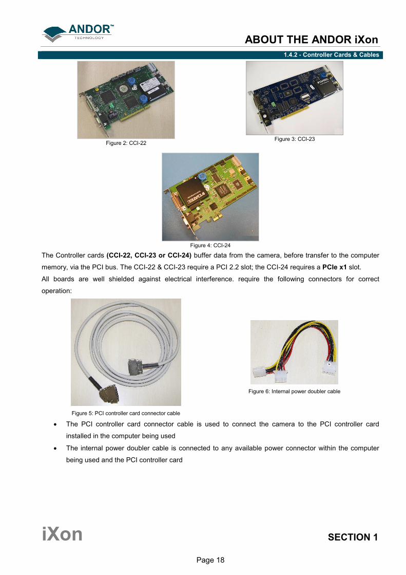
1.4.2 - Controller Cards & Cables
Figure 2: CCI-22
Figure 3: CCI-23
Figure 4: CCI-24
The Controller cards (CCI-22, CCI-23 or CCI-24) buffer data from the camera, before transfer to the computer
memory, via the PCI bus. The CCI-22 & CCI-23 require a PCI 2.2 slot; the CCI-24 requires a PCIe x1 slot.
All boards are well shielded against electrical interference. require the following connectors for correct
operation:
Figure 5: PCI controller card connector cable
Figure 6: Internal power doubler cable
• The PCI controller card connector cable is used to connect the camera to the PCI controller card
installed in the computer being used
• The internal power doubler cable is connected to any available power connector within the computer
being used and the PCI controller card

ABOUT THE ANDOR iXon
iXon SECTION 1
Page 19
1.4.3 - Power Supply Block
The cooler Power Supply Block (PSB) is used to supply power to the Thermoelectric cooler within the camera.
A 2.1 mm Jack connector links the detector head to the PSB.
NOTE: Cooling is only available when the PSB is connected to the camera.
1.4.4 - Mounting posts
A bag containing two Ø1/2" x 80mm long x1/4-20unc posts is included with all kits. These mounting posts can
be fitted on three sides of the camera that can be used to mount the camera if the C-Mount is not used, or to
mount accessories. There are 3 pairs of holes for the mounting posts, each with 2.0" spacing. These are easily
fitted as shown in Figure 7:
Figure 7: Mounting post installation
1.4.5 - Optional Extras
The following items can also be added to the system as necessary:
• C-Mount Lens
• C-Mount Lens Adaptor
• F-Mount Lens
• F-Mount Lens Adaptor
• Mounting Posts

ABOUT THE ANDOR iXon
iXon SECTION 1
Page 20
1.5 - SAFETY PRECAUTIONS
1.5.1 - Statement regarding equipment operation
IF THE EQUIPMENT IS USED IN A MANNER NOT SPECIFIED BY ANDOR TECHNOLOGY plc, THE
PROTECTION PROVIDED BY THE EQUIPMENT MAY BE IMPAIRED.
1.5.2 - Working with electronics
The computer equipment that is to be used to operate the iXon CCD Detector should be fitted with appropriate
surge/EMI/RFI protection on all power lines. Dedicated power lines or line isolation may be required for some
extremely noisy sites. Appropriate static control procedures should be used during the installation of the
system. Attention should be given to grounding. All cables should be fastened securely into place in order to
provide a reliable connection and to prevent accidental disconnection. The power supply to the computer
system should be switched off when changing connections between the computer and the Detector Head. The
computer manufacturer’s safety precautions should be followed when installing the Interface Card into the
computer. The circuits used in the detector head and the interface card are extremely sensitive to static
electricity and radiated electromagnetic fields, and therefore they should not be used, or stored, close to
EMI/RFI generators, electrostatic field generators, electromagnetic or radioactive devices, or other similar
sources of high energy fields. The types of equipment that can cause problems include the following:
• Arc welders
• Plasma sources
• Pulsed discharge optical sources
• Radio frequency generators
• X-ray instruments
If shielding is inadequate, operation of the system close to intense pulsed sources (arc lamps, lasers, xenon
strobes, etc.) may compromise performance.
1.5.2.1 - Special note on Controller Card
WARNING: Pins 11, 12 & 13 are RESERVED and are not available for auxiliary use. Do not make
electrical connections to these pin locations when attaching external devices via the Controller Card
Auxiliary Connector port or damage may occur to the Controller card, the Detector Head or your
external device.

ABOUT THE ANDOR iXon
iXon SECTION 1
Page 21
1.5.3 - Care of the Detector Head
1. YOUR DETECTOR IS A PRECISION SCIENTIFIC INSTRUMENT CONTAINING FRAGILE
COMPONENTS. ALWAYS HANDLE WITH THE CARE ACCORDED TO ANY SUCH INSTRUMENT.
2. THERE ARE NO USER-SERVICEABLE PARTS INSIDE THE DETECTOR HEAD. A NUMBER OF
SCREWS ON THE DETECTOR HEAD HAVE BEEN MARKED WITH RED PAINT TO PREVENT
TAMPERING. IF YOU ADJUST THESE SCREWS YOUR WARRANTY WILL BE VOID.
3. NEVER USE WATER THAT HAS BEEN CHILLED BELOW THE DEW POINT OF THE AMBIENT
ENVIRONMENT TO COOL THE DETECTOR.
You may see condensation on the outside of the detector body if the cooling water is at too low a temperature
or if the water flow is too great. The first signs of condensation will usually be visible around the connectors
where the water tubes are attached. In such circumstances switch off the system, and wipe the detector head
with a soft, dry cloth. It is likely there will already be condensation on the cooling block and cooling fins inside
the detector head. Set the detector head aside to dry for several hours before you attempt reuse. Before reuse
blow dry gas through the cooling slits on the side of the detector head to remove any residual moisture. Use
warmer water or reduce the flow of water when you start using the device again.
NOTE: Please refer to pages 22 - 25 for details of minimum achievable temperatures and important
advice on avoiding overheating.

ABOUT THE ANDOR iXon
iXon SECTION 1
Page 22
1.5.4 - Cooling
The CCD is cooled using a thermoelectric (TE) cooler. TE coolers are small, electrically powered devices with
no moving parts, making them reliable and convenient. A TE cooler is actually a heat pump, i.e.it achieves a
temperature difference by transferring heat from its ‘cold side’ (the CCD-chip) to its ‘hot side’ (the built-in heat
sink). Therefore the minimum absolute operating temperature of the CCD depends on the temperature of the
heat sink. Our vacuum design means that we can achieve a maximum temperature difference of over 110ºC
(DU models with optional PS-25), a performance unrivalled by other systems. The maximum temperature
difference that a TE device can attain is dependent on the following factors:
• Heat load created by the CCD
• Number of cooling stages of the TE cooler
• Operating current.
The heat that builds up on the heat sink must be removed. This can be done in one of two ways:
1. Air cooling: a small built-in fan forces air over the heat sink.
2. Water cooling: external water is circulated through the heat sink using the water connectors on
the top of the head.
All Andor CCD systems support both cooling options. Whichever method is being used, it is not desirable for the
operating temperature of the CCD simply to be dependent on, or vary with the heat sink temperature. Therefore
a temperature sensor on the CCD, combined with a feedback circuit that controls the operating current of the
cooler, allows stabilisation of the CCD to any desired temperature within the cooler operating range. NOTE: In
order to achieve the maximum cooling performance specified for your iXon CCD, you must use the PSB
which has been supplied with your system.
Whichever cooling method you are using, make sure that the detector head does not overheat, as this can
cause system failure. Overheating may occur if:
• The air vents on the sides of the head are accidentally blocked or there is insufficient or no water flow
• You are using air cooling with the optional PS-25 and have selected Deep Cooling. Air cooling may not
be possible if the ambient air temperature is over 20ºC.
To protect the detector from overheating, a thermal switch has been attached to the heat sink. If the
temperature of the heat sink rises above 47ºC, the current supply to the cooler will cut out and a buzzer will
sound. Once the head has cooled, the cut-out will automatically reset. It is not recommended that you operate
in conditions that would cause repeated cut-outs as the thermal switch has a limited number of operations.
NOTE: Never block the air vents on the detector head.

ABOUT THE ANDOR iXon
iXon SECTION 1
Page 23
1.5.4.1 - Air cooling
Air cooling is the most convenient method of cooling, but it will not achieve as low an operating temperature as
water cooling (see below). Even with a fan (see note immediately below), a heat sink typically needs to be 10ºC
hotter than the air (room) temperature to transfer heat efficiently to the surrounding air. Therefore the minimum
CCD temperature that can be achieved will be dependent on the room temperature. Table1 below is a guide to
the minimum CCD operating temperatures for various air temperatures and it should be noted that performance
of individual systems will vary slightly.
NOTE: The fan does not operate until the heat sink temperature has reached between 20ºC and 22ºC. It
is therefore quite normal for the fan not to operate when the system is first switched on. Please also
refer to pages 37 - 39 for information on temperature & fan settings.
Table 1: Evacuated housing - High performance air cooling with power supply block
Air Temperature External PSU box
20ºC -60ºC
25ºC -58ºC
30ºC -56ºC
NOTES:
1. The relationship between the air temperature and the minimum CCD temperature in the table is
not linear. This is because TE coolers become less efficient as they get colder.
2. Systems are specified in terms of the minimum dark current achievable, rather than Absolute
Temperature. For dark current specifications, please refer to the specification sheet for your
camera.
3. Cooling the CCD detector helps you reduce dark signal and its associated shot noise. Cooling
will also affect the Electron Multiplying Gain of the iXon CCD.

ABOUT THE ANDOR iXon
iXon SECTION 1
Page 24
1.5.4.2 - Water cooling
A flow of water through the heat sink removes heat very efficiently, since the heat sink is never more than 1ºC
hotter than the water. With this type of cooling, the minimum temperature of the CCD will be dependent only on
the water temperature and not on the room temperature. Table 2 below is a guide to the minimum CCD
operating temperatures for various water temperatures and it should be noted that performance of individual
systems will vary slightly.
Water cooling, either chilled though a refrigeration process or re-circulated (which is water forced air cooled
then pumped) allows lower minimum operating temperatures than air cooling. However, there is a very
important point relating to water cooling. If the water temperature is lower than the dew point of the room,
condensation will occur on the heat sink, the water taps and other metal parts of the head. This will quickly
destroy the head and must never be allowed to happen. However this is not an issue when using a
Recirculator which eliminates the dew point problem. NOTE: Never use cooling water that is colder than
the dew point of the air in the room. Damage caused in this way is not covered by the warranty.
Table 2: Evacuated housing - High performance water cooling with power supply block
Water Temperature External PSU box
10oC -75°C
15oC -73°C
20oC -71°C
25oC -69°C
ABOUT THE ANDOR iXon
iXon SECTION 1
Page 25
1.5.4.3 - Dew point
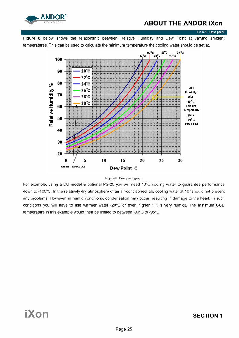
Figure 8 below shows the relationship between Relative Humidity and Dew Point at varying ambient
temperatures. This can be used to calculate the minimum temperature the cooling water should be set at.
Figure 8: Dew point graph
For example, using a DU model & optional PS-25 you will need 10ºC cooling water to guarantee performance
down to -100ºC. In the relatively dry atmosphere of an air-conditioned lab, cooling water at 10º should not present
any problems. However, in humid conditions, condensation may occur, resulting in damage to the head. In such
conditions you will have to use warmer water (20ºC or even higher if it is very humid). The minimum CCD
temperature in this example would then be limited to between -90ºC to -95ºC.
INSTALLATION
iXon SECTION 2
Page 26
SECTION 2 - INSTALLATION 2.1 - PC REQUIREMENTS
The system requires a PCI-compatible computer. The PCI slot you use must have bus master capability. The
minimum recommended specification is:
• 2.4 GHz Pentium Processor (or better)
• 1GB of RAM
• Minimum 10,000 RPM Hard drive (RAID 15,000 RPM preferred for extended Kinetic series)
• 32 MB free Hard Disc space.
• Auxiliary internal power connector available
• Windows 2000 or XP
The PCI Controller Card is installed as you would other slot-in cards such as graphics cards. NOTE: Please
consult the manual supplied with your personal computer to ensure correct installation of the
Controller Card for your particular PC.

INSTALLATION
iXon SECTION 2
Page 27
2.2 - INSTALLING THE CONTROLLER CARD
The PCI Controller Card is installed in the same manner as you would fit most other slot-in cards such as
graphics cards. NOTE: Please consult the manual supplied with your computer to ensure correct
installation of the controller card for your particular model. We recommend you perform the installation
in a similar manner to the following:
1. Power down the computer and any accessories.
2. Unplug the computer and any accessories from the wall outlet(s).
3. Whilst observing appropriate static control procedures, unplug all cables from the rear of the computer.
4. Unscrew any cover mounting screws on the computer and set them aside safely.
5. Carefully remove the cover of the computer, e.g.:
6. Situated inside the computer are a number of Expansion Slots, e.g.:
7. After deciding which slot you are going to use, remove any metal filler bracket(s) that may be covering
the opening for the slot at the back of the computer. Place any retaining screw(s) and/or clip(s) in a safe
container, as you will need them later in the installation procedure.
8. At this point, put on the ESD wrist strap supplied with your camera and attach the crocodile clip
to a suitable earth point on the PC e.g.:
9. IMPORTANT NOTE: The ESD strap must be worn at all times when handling the Controller Card.
10. Remove the Controller Card carefully from its protective packaging

INSTALLATION
iXon SECTION 2
Page 28
11. Firmly press the connector into the chosen expansion slot, e.g.:
12. For maximum cooling, when the supplied PCI card has an Auxiliary Power connector (“flylead”), this
can be connected to a suitable point on the power supply of the PC, e.g.:
NOTE: Should any problems be experienced with this connection, please contact your nearest technical
representative.
13. Making sure that the card’s mounting bracket is flush with any other mounting brackets or filler brackets
to either side of it, secure the Controller Card in place.
14. Replace the cover of the computer and secure it with the mounting screws if applicable.
15. Reconnect any accessories you were using previously.
INSTALLATION
iXon SECTION 2
Page 29
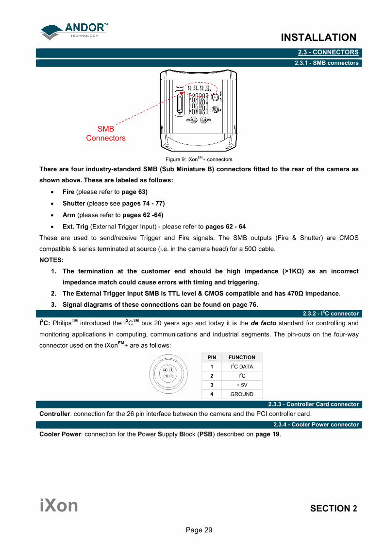
2.3 - CONNECTORS
2.3.1 - SMB connectors
Figure 9: iXonEM
+ connectors
There are four industry-standard SMB (Sub Miniature B) connectors fitted to the rear of the camera as
shown above. These are labeled as follows:
• Fire (please refer to page 63)
• Shutter (please see pages 74 - 77)
• Arm (please refer to pages 62 -64)
• Ext. Trig (External Trigger Input) - please refer to pages 62 - 64
These are used to send/receive Trigger and Fire signals. The SMB outputs (Fire & Shutter) are CMOS
compatible & series terminated at source (i.e. in the camera head) for a 50Ω cable.
NOTES:
1. The termination at the customer end should be high impedance (>1KΩ) as an incorrect
impedance match could cause errors with timing and triggering.
2. The External Trigger Input SMB is TTL level & CMOS compatible and has 470Ω impedance.
3. Signal diagrams of these connections can be found on page 76. 2.3.2 - I
2C connector
I2C: Philips
TM introduced the I
2C
TM bus 20 years ago and today it is the de facto standard for controlling and
monitoring applications in computing, communications and industrial segments. The pin-outs on the four-way
connector used on the iXonEM
+ are as follows:
PIN FUNCTION
1 I2C DATA
2 I2C
3 + 5V
4 GROUND
2.3.3 - Controller Card connector
Controller: connection for the 26 pin interface between the camera and the PCI controller card.
2.3.4 - Cooler Power connector
Cooler Power: connection for the Power Supply Block (PSB) described on page 19.
SMB Connectors
INSTALLATION
iXon SECTION 2
Page 30
2.4 - WATER PIPE CONNECTORS
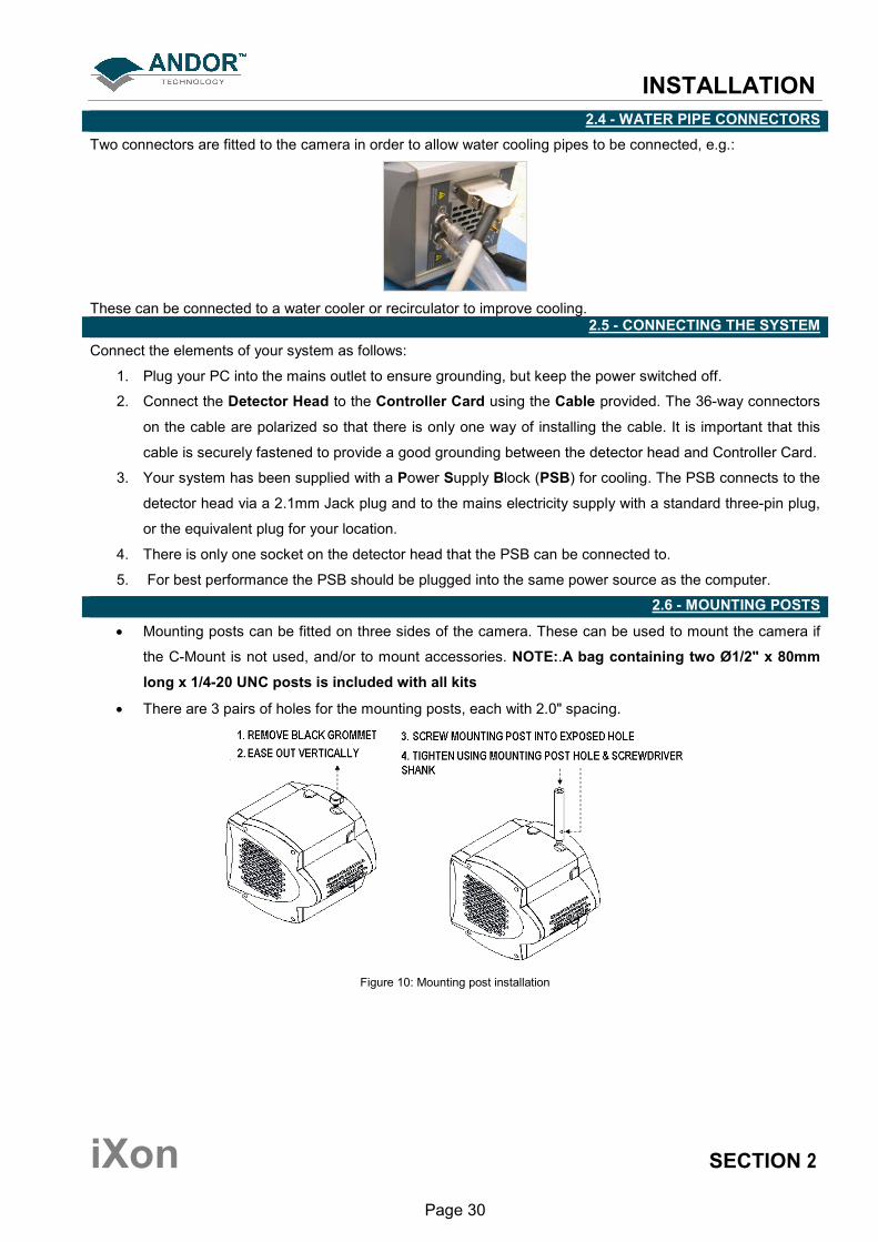
Two connectors are fitted to the camera in order to allow water cooling pipes to be connected, e.g.:
These can be connected to a water cooler or recirculator to improve cooling. 2.5 - CONNECTING THE SYSTEM
Connect the elements of your system as follows:
1. Plug your PC into the mains outlet to ensure grounding, but keep the power switched off.
2. Connect the Detector Head to the Controller Card using the Cable provided. The 36-way connectors
on the cable are polarized so that there is only one way of installing the cable. It is important that this
cable is securely fastened to provide a good grounding between the detector head and Controller Card.
3. Your system has been supplied with a Power Supply Block (PSB) for cooling. The PSB connects to the
detector head via a 2.1mm Jack plug and to the mains electricity supply with a standard three-pin plug,
or the equivalent plug for your location.
4. There is only one socket on the detector head that the PSB can be connected to.
5. For best performance the PSB should be plugged into the same power source as the computer.
2.6 - MOUNTING POSTS
• Mounting posts can be fitted on three sides of the camera. These can be used to mount the camera if
the C-Mount is not used, and/or to mount accessories. NOTE:.A bag containing two Ø1/2" x 80mm
long x 1/4-20 UNC posts is included with all kits
• There are 3 pairs of holes for the mounting posts, each with 2.0" spacing.
Figure 10: Mounting post installation
INSTALLATION
iXon SECTION 2
Page 31
2.7 - INSTALLING THE SOFTWARE
During the start up sequence the operating system will detect the Andor plug-in card and a dialogue box will
prompt you for the location of the device driver.
1. Insert the Andor CD and navigate to the Setup Information File (atsolis.inf). Select the device driver
file then click OK.
2. The ‘installation wizard’ now starts. (If it does not start automatically, run \setup.exe on the CD.) Follow
the on-screen prompts. Remove the CD and then restart the computer to complete the installation.
3. Run the Andor application: from the PC’s desktop select Start…Programs…Andor iXon. …Andor
iXon. .

USING THE iXon
iXon SECTION 3
Page 32
SECTION 3 - USING THE iXon 3.1 - STARTING THE APPLICATION
On the desktop, click on the icon which is installed during the installation process and the Solis Splash
Screen appears briefly:
The Main Window then appears, e.g.:
USING THE iXon
iXon SECTION 3
Page 33
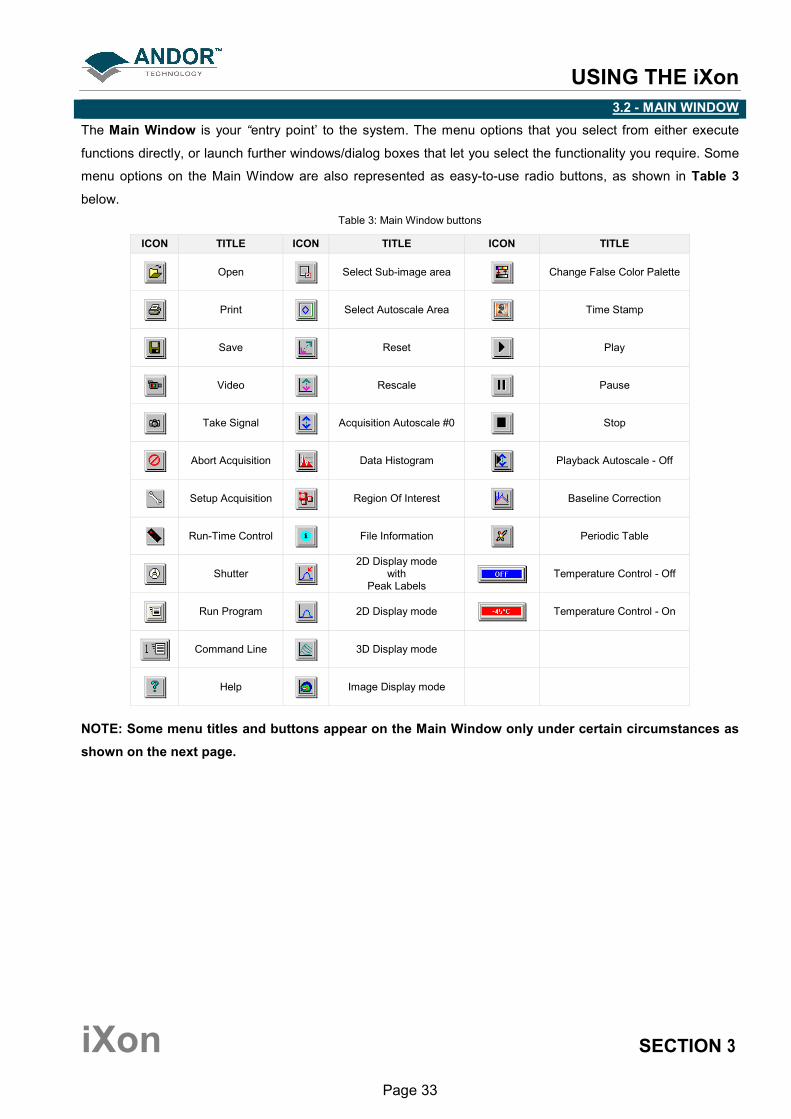
3.2 - MAIN WINDOW
The Main Window is your “entry point’ to the system. The menu options that you select from either execute
functions directly, or launch further windows/dialog boxes that let you select the functionality you require. Some
menu options on the Main Window are also represented as easy-to-use radio buttons, as shown in Table 3
below.
Table 3: Main Window buttons
ICON TITLE ICON TITLE ICON TITLE
Open
Select Sub-image area
Change False Color Palette
Select Autoscale Area
Time Stamp
Save
Reset
Play
Video
Rescale
Pause
Take Signal
Acquisition Autoscale #0
Stop
Abort Acquisition
Data Histogram
Playback Autoscale - Off
Setup Acquisition
Region Of Interest
Baseline Correction
Run-Time Control
File Information
Periodic Table
Shutter
2D Display mode with
Peak Labels Temperature Control - Off
Run Program
2D Display mode Temperature Control - On
Command Line
3D Display mode
Help
Image Display mode
NOTE: Some menu titles and buttons appear on the Main Window only under certain circumstances as
shown on the next page.
USING THE iXon
iXon SECTION 3
Page 34
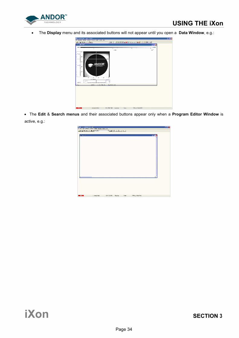
• The Display menu and its associated buttons will not appear until you open a Data Window, e.g.:
• The Edit & Search menus and their associated buttons appear only when a Program Editor Window is
active, e.g.:

USING THE iXon
iXon SECTION 3
Page 35
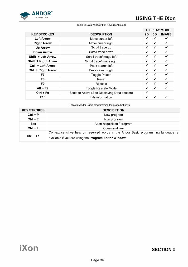
3.3 - HOT KEYS
Hot keys (or shortcuts) as shown in Tables 2, 3 & 4 enable you to work with the system directly from the
keyboard, rather than via the mouse.
Table 4: Data Acquisition Hot Keys
KEY STROKE DESCRIPTION
F5 Take signal
F6 Autoscale Acquisition
Ctrl + B Take background
Ctrl + R Take reference
Esc Abort Acquisition
Table 5: Data Window Hot Keys
DISPLAY MODE
KEY STROKES DESCRIPTION 2D 3D IMAGE
+ Expand (‘Stretch’) data-axis
- Contract (‘Shrink’) data-axis
Ins If maintain aspect ratio off, expand x-axis.
If maintain aspect ratio on, expand x-axis and y-axis
Del If maintain aspect ratio off, contract x-axis.
If maintain aspect ratio on, contract x-axis and y-axis.
/
On image, if maintain aspect ratio off, expand y-axis. On image, if maintain aspect ratio on, expand x-axis and y-axis.
Home Move cursor furthest left
End Move cursor furthest right
PgUp Scroll up through tracks
PgDn Scroll down through tracks
Shift + PgUp Move to next image in series
Shift + PgDn Move to previous image in series
Left Arrow Move cursor left
Right Arrow Move cursor right
Up Arrow Scroll trace up (on image: move cursor up)
Down Arrow Scroll trace down (on image: move cursor down)
Shift + Left Arrow Scroll trace/image left
Shift + Right Arrow Scroll trace/image right
Ctrl + Left Arrow Peak search left
Ctrl + Right Arrow Peak search right
USING THE iXon
iXon SECTION 3
Page 36
Table 5: Data Window Hot Keys (continued)
DISPLAY MODE
KEY STROKES DESCRIPTION 2D 3D IMAGE
Left Arrow Move cursor left
Right Arrow Move cursor right
Up Arrow Scroll trace up (on image: move cursor up)
Down Arrow Scroll trace down (on image: move cursor down)
Shift + Left Arrow Scroll trace/image left
Shift + Right Arrow Scroll trace/image right
Ctrl + Left Arrow Peak search left
Ctrl + Right Arrow Peak search right
F7 Toggle Palette
F8 Reset
F9 Rescale
Alt + F9 Toggle Rescale Mode
Ctrl + F9 Scale to Active (See Displaying Data section)
F10 File information
Table 6: Andor Basic programming language hot keys
KEY STROKES DESCRIPTION
Ctrl + P New program
Ctrl + E Run program
Esc Abort acquisition / program
Ctrl + L Command line
Ctrl + F1 Context sensitive help on reserved words in the Andor Basic programming language is
available if you are using the Program Editor Window.

PRE-ACQUISITION
iXon SECTION 4
Page 37
SECTION 4 - PRE-ACQUISITION 4.1 - SETTING TEMPERATURE
For accurate readings, the CCD should first be cooled, as this will help reduce dark signal and associated shot
noise. To do this, either select the Temperature option from the Hardware drop-down menu on the Main
Window:
or click the button in the bottom-left of the screen.
This will open up the Temperature Control dialog box :
Select On in the Cooler check box.

PRE-ACQUISITION
iXon SECTION 4
Page 38
The Degrees (C) field in the Temperature Setting section will now be highlighted in blue and the Cooler will
be indicated as On, e.g.:
To adjust the temperature, either type in the new figure in the Degrees (C) box or slide the arrowed bar down or
up. Once the desired temperature has been selected, click OK. The dialog box will disappear and the
Temperature Control button in the bottom-left of the screen will show the current temperature highlighted in
red e.g.:
This figure will change as the head cools. Once the head has reached the desired temperature, the highlighted
area changes to blue. You can also select the option to have the Cooler is on as soon as you start the
application. This is selectable in the bottom-left of the Temperature dialog box.
PLEASE REFER TO PAGES 22 - 25 FOR DETAILS OF MINIMUM ACHIEVABLE TEMPERATURES AND
IMPORTANT ADVICE ON AVOIDING OVERHEATING.
PRE-ACQUISITION
iXon SECTION 4
Page 39
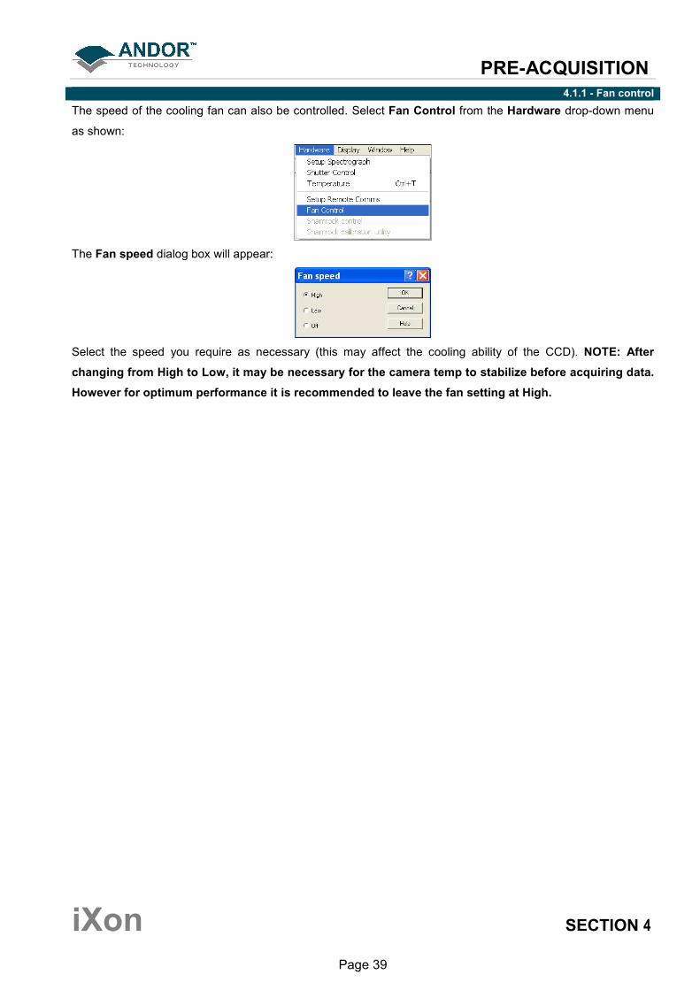
4.1.1 - Fan control
The speed of the cooling fan can also be controlled. Select Fan Control from the Hardware drop-down menu
as shown:
The Fan speed dialog box will appear:
Select the speed you require as necessary (this may affect the cooling ability of the CCD). NOTE: After
changing from High to Low, it may be necessary for the camera temp to stabilize before acquiring data.
However for optimum performance it is recommended to leave the fan setting at High.
PRE-ACQUISITION
iXon SECTION 4
Page 40
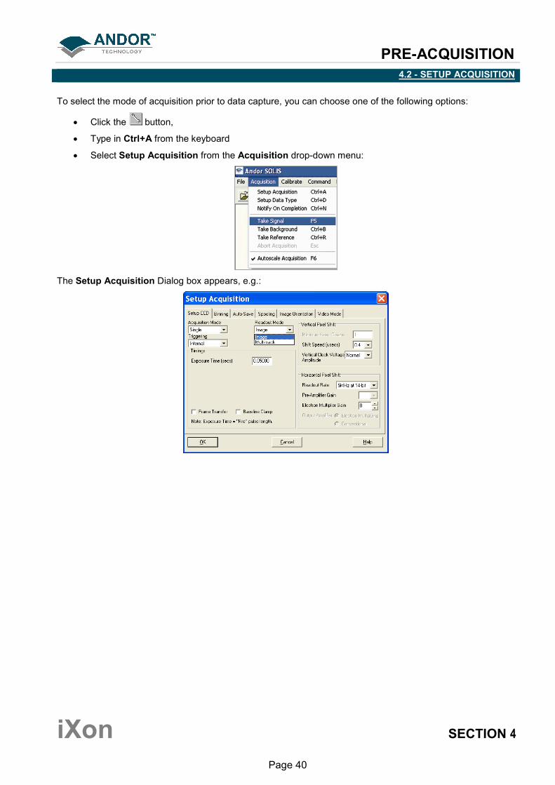
4.2 - SETUP ACQUISITION
To select the mode of acquisition prior to data capture, you can choose one of the following options:
• Click the button,
• Type in Ctrl+A from the keyboard
• Select Setup Acquisition from the Acquisition drop-down menu:
The Setup Acquisition Dialog box appears, e.g.:
PRE-ACQUISITION
iXon SECTION 4
Page 41
As you select an Acquisition Mode you will notice that you are able to enter additional exposure-related
parameters in a column of text boxes. Appropriate text boxes become active as you select each Acquisition
Mode.
The value you enter in one text box may affect the value in another text box. The following matrix lists the
Acquisition Modes and for each mode indicates the parameters for which you may enter a value in the
appropriate text box:
Mode
Exposure Time
Accumulate Cycle Time
No. of
Accumulations
Kinetic Cycle Time
No. in Kinetic Series
Single Scan
Accumulate
Kinetic

PRE-ACQUISITION
iXon SECTION 4
Page 42
4.2.1 - Run Time control
The Run Time Control provides the user with the ability to control the following parameters using slider
controls:
• EM Gain
• Exposure time of the CCD
The controls are activated by clicking on the button on the Main Window. When selected, the dialog box
appears, e.g.:
Each dialog box has sliders that can be moved up and down to control the required parameters and there are
three levels of control:
• Single-Step
• Fine
• Coarse
The controls can also be accessed either by using the relevant buttons on the Remote Control (see page 45)
or by moving the windows pointer with the mouse or the remote control unit (if attached). The gauge that is
active has its name highlighted in green and the actual setting of each gauge is given in the text boxes below
them.
• The EM Gain gauge can be varied from a setting of 0 to 255
• The Exposure gauge can be varied from the minimum exposure setting
Note: The exposure gauge upper limit will auto-range as the setting is increased.

PRE-ACQUISITION
iXon SECTION 4
Page 43
When the Control section is selected for Mouse, the Single-Step, Fine & Coarse selectors are removed and
the slider titles are no longer highlighted in green, e.g.:
While the remote is being used to access the Run Time Control dialog box, the Trigger on the underside of the
Remote Control is used to make or cancel an acquisition. It has the same function as pressing the green Take
Signal button or the red Cancel Take Signal on the toolbar of the main window.
PRE-ACQUISITION
iXon SECTION 4
Page 44
4.2.2 - Remote control
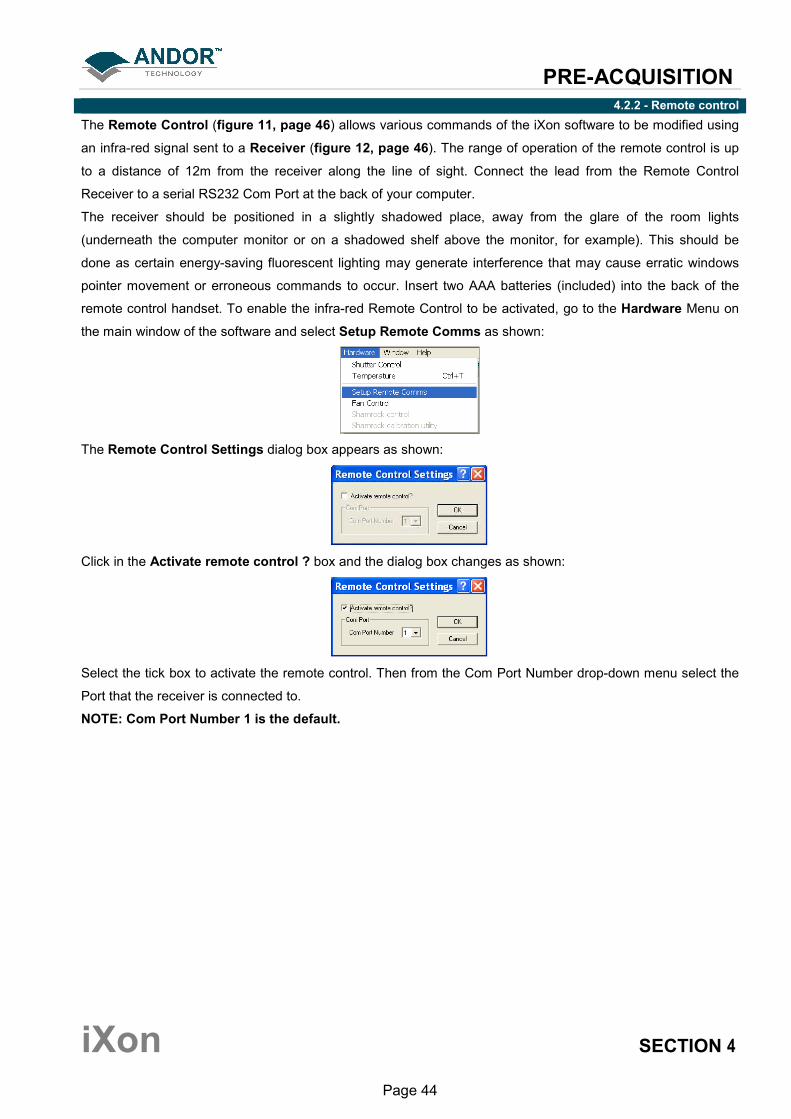
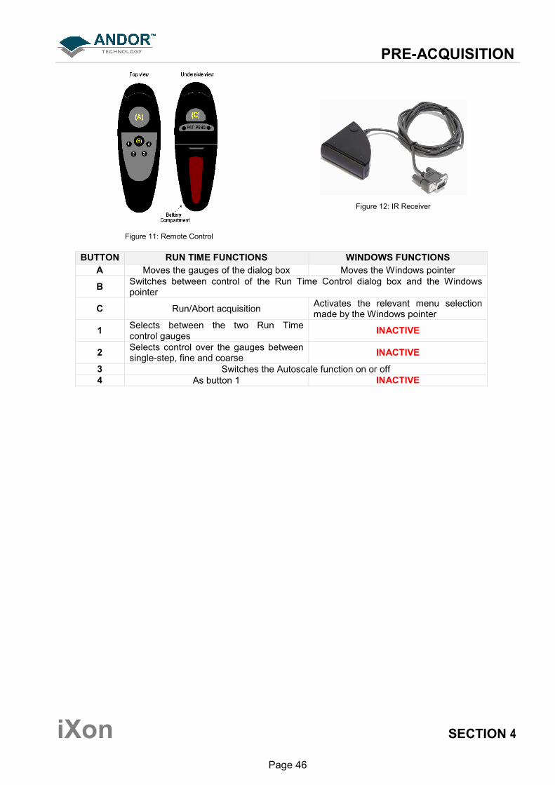
The Remote Control (figure 11, page 46) allows various commands of the iXon software to be modified using
an infra-red signal sent to a Receiver (figure 12, page 46). The range of operation of the remote control is up
to a distance of 12m from the receiver along the line of sight. Connect the lead from the Remote Control
Receiver to a serial RS232 Com Port at the back of your computer.
The receiver should be positioned in a slightly shadowed place, away from the glare of the room lights
(underneath the computer monitor or on a shadowed shelf above the monitor, for example). This should be
done as certain energy-saving fluorescent lighting may generate interference that may cause erratic windows
pointer movement or erroneous commands to occur. Insert two AAA batteries (included) into the back of the
remote control handset. To enable the infra-red Remote Control to be activated, go to the Hardware Menu on
the main window of the software and select Setup Remote Comms as shown:
The Remote Control Settings dialog box appears as shown:
Click in the Activate remote control ? box and the dialog box changes as shown:
Select the tick box to activate the remote control. Then from the Com Port Number drop-down menu select the
Port that the receiver is connected to.
NOTE: Com Port Number 1 is the default.
PRE-ACQUISITION
iXon SECTION 4
Page 45
The remote control has two modes of operation.
1. The first mode provides direct control over the Run Time Control dialog box (see Run-Time control on
pages 42 - 43) where the following parameters may be varied:
Autoscale ON/OFF
EM Gain
Exposure Time
Run/Abort acquisition
Note: Gain and Exposure Time may also be modified using the Setup Acquisition Dialog Box.
2. The second mode of operation allows the remote to be used as a general tool for moving the Windows
pointer around and accessing all the various menus and dialog boxes of both the iXon software and the
general Windows interface.
PRE-ACQUISITION
iXon SECTION 4
Page 46
Figure 11: Remote Control
Figure 12: IR Receiver
BUTTON RUN TIME FUNCTIONS WINDOWS FUNCTIONS
A Moves the gauges of the dialog box Moves the Windows pointer
B Switches between control of the Run Time Control dialog box and the Windows pointer
C Run/Abort acquisition Activates the relevant menu selection made by the Windows pointer
1 Selects between the two Run Time control gauges
INACTIVE
2 Selects control over the gauges between single-step, fine and coarse
INACTIVE
3 Switches the Autoscale function on or off
4 As button 1 INACTIVE

PRE-ACQUISITION
iXon SECTION 4
Page 47
4.3 - SPOOLING
The Andor Solis software has an extensive range of options that allow you to spool acquisition data direct to the
hard disk of your PC. This is particularly useful when acquiring a series of many images. The amount of data
generated by a Kinetic Series of, for example 1000 acquisitions, is huge and more than most PC RAM
can handle.
To select click on the Spooling tab and the Spooling dialog box appears e.g.:
With the spooling function enabled, data is written directly to the hard disk of you PC, as it is being acquired. To
enable the spooling function on your software, tick the Enable Spooling box. You must also enter a
stem name, and also select a location for the for this spooled data file, e.g.:
NOTE: Spooling large amounts of data straight to hard disk for later retrieval requires a hard disk of
sufficient read-write speed. Andor recommends only very high-speed hard disk drives be used for this
type of operation and these need to be dedicated for Spooling.
PRE-ACQUISITION
iXon SECTION 4
Page 48
4.3.1 - Virtual Memory
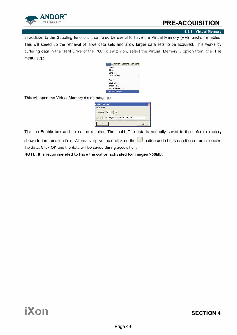
In addition to the Spooling function, it can also be useful to have the Virtual Memory (VM) function enabled.
This will speed up the retrieval of large data sets and allow larger data sets to be acquired. This works by
buffering data in the Hard Drive of the PC. To switch on, select the Virtual Memory… option from the File
menu, e.g.:
This will open the Virtual Memory dialog box,e.g.:
Tick the Enable box and select the required Threshold. The data is normally saved to the default directory
shown in the Location field. Alternatively, you can click on the button and choose a different area to save
the data. Click OK and the data will be saved during acquisition.
NOTE: It is recommended to have the option activated for images >50Mb.

PRE-ACQUISITION
iXon SECTION 4
Page 49
4.4 - AUTO-SAVE
Auto-Save allows you to set parameters and controls for the auto saving of acquisition files thus removing the
worry of lost data and files. To select, click on the Auto-Save tab on the Setup Acquisition dialog box The Auto-
save dialog box appears, e.g.:
Tick the Enable Auto-Save box. If selected, acquisitions will be saved automatically when each one is
completed. Each subsequent auto-saved file will over-write the previously auto-saved one.
There is also an Auto-Increment On/Off tick box. This allows a number to also be appended to the main Stem
Name. This number is automatically incremented each time a file is saved. This time the auto-saved files will
not overwrite any previous auto-saved files. In the Auto-Save dialog box, a Stem Name may be entered. This is
the main root of the name that the acquisition is to be saved as.
The Stem Name can be appended with a number of details as follows:
• Date
• Computer name
• Camera type
• Time
• Operator name (supplied by user)
• Separator
Any combination of these may be selected by activating the relevant tick box.
NOTE: This function will only Auto-Save Single Scan, Kinetic Series, Fast Kinetics or Accumulated
images, not data acquired in Video mode.

ACQUIRING DATA
iXon SECTION 5
Page 50
SECTION 5 - ACQUIRING DATA 5.1 - INITIAL ACQUISITION
To start an initial data acquisition you can either:
• Click the button on the Main Window
• Press F5 on the keyboard
• Select the Take Signal option from the Acquisition drop-down menu, e.g.:
The Data Window opens (labeled #0 Acquisition) and displays the acquired data, according to the parameters
selected on the Setup Acquisition Dialog box. e.g.:
ACQUIRING DATA
iXon SECTION 5
Page 51
When you acquire data, by reading out a scan or a series of scans of the CCD-chip at the heart of the detector,
the data are stored together in a Data Set, which exists in your computer’s Random Access Memory (RAM) or
on its Hard Disk. You can also create a data set via the Andor Basic programming language. #n uniquely
identifies the data set while the data set is being displayed and is temporary. It ceases to be associated with the
data set once you close all data windows bearing the same #n. It is often referred to as an Acquisition
Window.
NOTE: Each Data Window has the same name and #n (which identify the data set), but a unique
number, following the data set name, to identify the window itself. Data can be modified only in a Data
Window labeled with the name and the #n of the data set to which the data belong. If you modify a data
set and attempt to close the data window, you will be prompted to save the data set to file.
If you have selected Accumulate or Kinetic as the Acquisition Mode, new data will continue to be acquired and
displayed until you carry out one of the following actions:
• Select Abort Acquisition from the Acquisition drop-down menu.
• Click the button
• Press the <ESC> key.
This stops any data capture process that may be under way. Information on how to capture & view more
detailed data is contained in the pages that follow.
ACQUIRING DATA
iXon SECTION 5
Page 52
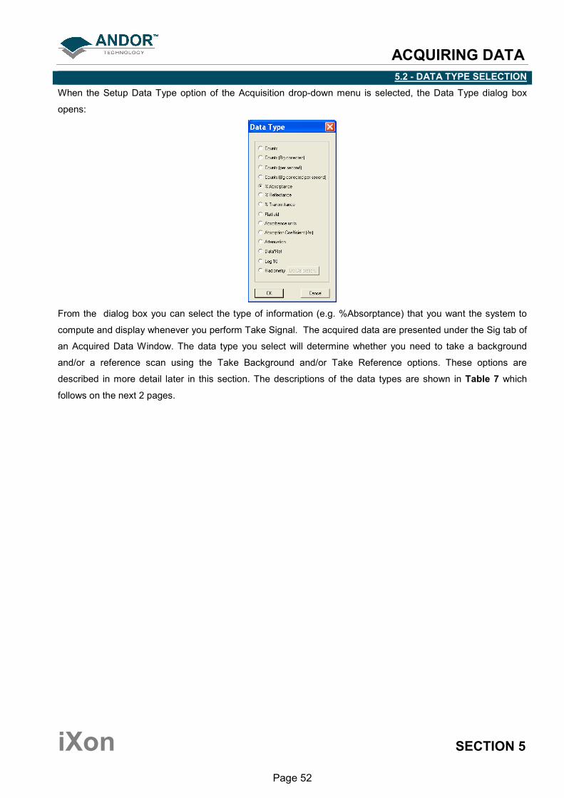
5.2 - DATA TYPE SELECTION
When the Setup Data Type option of the Acquisition drop-down menu is selected, the Data Type dialog box
opens:
From the dialog box you can select the type of information (e.g. %Absorptance) that you want the system to
compute and display whenever you perform Take Signal. The acquired data are presented under the Sig tab of
an Acquired Data Window. The data type you select will determine whether you need to take a background
and/or a reference scan using the Take Background and/or Take Reference options. These options are
described in more detail later in this section. The descriptions of the data types are shown in Table 7 which
follows on the next 2 pages.
ACQUIRING DATA
iXon SECTION 5
Page 53
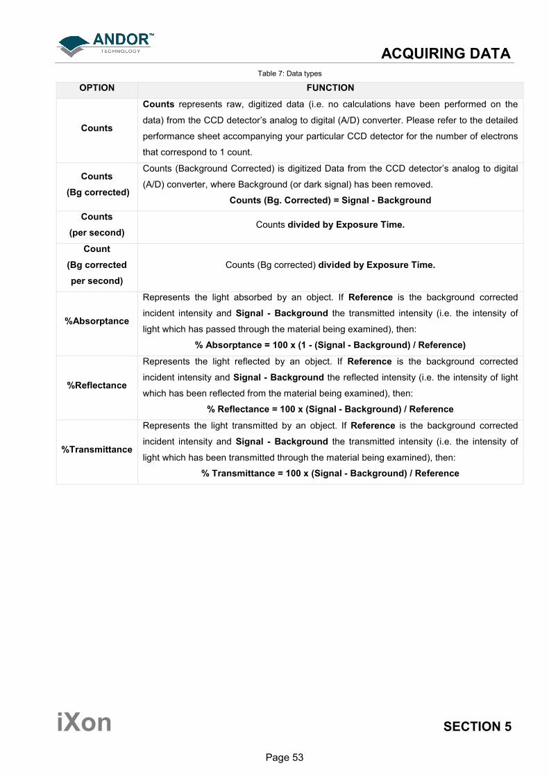
Table 7: Data types
OPTION FUNCTION
Counts
Counts represents raw, digitized data (i.e. no calculations have been performed on the
data) from the CCD detector’s analog to digital (A/D) converter. Please refer to the detailed
performance sheet accompanying your particular CCD detector for the number of electrons
that correspond to 1 count.
Counts
(Bg corrected)
Counts (Background Corrected) is digitized Data from the CCD detector’s analog to digital
(A/D) converter, where Background (or dark signal) has been removed.
Counts (Bg. Corrected) = Signal - Background
Counts
(per second) Counts divided by Exposure Time.
Count
(Bg corrected
per second)
Counts (Bg corrected) divided by Exposure Time.
%Absorptance
Represents the light absorbed by an object. If Reference is the background corrected
incident intensity and Signal - Background the transmitted intensity (i.e. the intensity of
light which has passed through the material being examined), then:
% Absorptance = 100 x (1 - (Signal - Background) / Reference)
%Reflectance
Represents the light reflected by an object. If Reference is the background corrected
incident intensity and Signal - Background the reflected intensity (i.e. the intensity of light
which has been reflected from the material being examined), then:
% Reflectance = 100 x (Signal - Background) / Reference
%Transmittance
Represents the light transmitted by an object. If Reference is the background corrected
incident intensity and Signal - Background the transmitted intensity (i.e. the intensity of
light which has been transmitted through the material being examined), then:
% Transmittance = 100 x (Signal - Background) / Reference

ACQUIRING DATA
iXon SECTION 5
Page 54
Table 7: Data types (continued)
OPTION FUNCTION
Flatfield
Flatfield is used to remove any pixel-to-pixel variations that are inherent in the CCD
sensor. If Reference is the background corrected incident intensity, the Signal is divided
by the Reference so:
Flatfield = M x Signal / Reference
where M is the Mean of Reference.
Absorbance
units
A measure of light absorbed by an object (i.e. they represent the object’s Optical Density -
OD). If Reference is the background corrected incident intensity and Signal -
Background the transmitted intensity (i.e. the intensity of light which has passed through
the material being examined), then Transmission = (Signal - Background) / Reference.
Absorbance Units are defined as Log10 (1 / Transmission).
Absorbance Units = Log10 (Reference / (Signal - Background))
Absorption
Coefficient (/m)
Indicates the internal absorptance of a material per unit distance (m). It is calculated as -
loge t, where t is the unit transmission of the material and loge is the natural logarithm. If
Reference is the background corrected incident intensity, and Signal - Background the
transmitted intensity (i.e. the intensity of light which has passed through the material being
examined), then:
Transmission = (Signal - Background) / Reference
Absorption Coefficient = -loge ((Signal - Background) / Reference)
Attenuation
A measurement, in decibels, of light absorbed due to transmission through a material -
decibels are often used to indicate light loss in fiber optic cables, for instance. If Reference
is the background corrected incident intensity, and Signal - Background the transmitted
intensity (i.e. the intensity of light which has passed through the material being examined),
then:
Attenuation = 10 x log10 ((Signal - Background) / Reference)
Data*Ref
Allows you to ‘custom modify’ the background corrected signal:
Data x Ref = (Signal - Background) x Reference Store Value
Please refer to the Andor Basic programming manual for similar operations.
Log 10 Calculates the logarithm to the base 10 of the background corrected signal counts.
Log Base 10 = log10 (Signal - Background)
Radiometry
(Optional extra)
Allows you to calculate values for radiance or irradiance. The system requires that you
supply calibration details. This option must be ordered separately. This option must be
ordered separately.

ACQUIRING DATA
iXon SECTION 5
Page 55
As an example, the system will compute % Absorptance as:
100 x (1 - (Signal - Background) / Reference).
The illustration below shows a typical use of Background, Reference and Signal for computations such as
%Absorptance or %Transmittance:
The default data type (used when you capture data and have not explicitly made a selection from the Data Type
dialog box) is Counts.
• If you select background corrected counts as your data type - Counts (Bg Corrected) - you will have to
perform Take Background before you perform Take Signal.
• If you select any data type other than Counts or Counts (Bg Corrected) you will have to perform Take
Background and Take Reference (in that order) before performing Take Signal.
The calculations for the various data types assume the following definitions:
Signal: data in uncorrected Counts, acquired via Take Signal.
Background: data in uncorrected Counts, acquired in darkness, via Take Background.
Reference: background corrected data, acquired (usually for the purpose of computing a
material’s reflection, transmission or absorption characteristics) via Take Reference.
Reference data are normally acquired from the light source, without the light having been
reflected from or having passed though the material being studied.
If you require raw or background corrected data pertaining to the light source itself, Signal will be data acquired
directly from the source.
If you intend to compute the reflection, transmission or absorption characteristics of a material, Signal will be
data acquired from light that has passed through or has been reflected from the material being studied.
NOTES:
1. ‘Signal’, as used in the definitions of the calculations, refers to ‘raw’ data from the CCD and
should not be confused with the possibly ‘processed’ data to be found under the Sig tab of the
Data Window.
2. Functionality for displaying and manipulating data is only available if a Data File has been
opened, if data have been newly acquired, or if you are using the Andor Basic programming
language to create a new window in which to display data. In each case data are displayed in a
data window.

ACQUIRING DATA
iXon SECTION 5
Page 56
5.3 - ACQUISITION TYPES
From the Acquisition drop-down menu on the Main Window, you can make the following data acquisition
selections:
• Take Signal
• Take Background
• Take Reference
Provided you do not change the acquisition parameters, the scans you take for background and reference are
automatically used for subsequent data acquisitions whenever you perform Take Signal.

ACQUIRING DATA
iXon SECTION 5
Page 57
5.3.1 - Take Signal (Autoscale Acquisition Off)
Autoscale Acquisition can be selected from the Acquisition drop-down menu as shown (or press F6 on the
keyboard):
With Autoscale Acquisition deselected, the display will remain the same size regardless of brightness settings,
etc. When selected off, the button appears (click this button to switch back on). 5.3.2 - Take Signal (Autoscale Acquisition On)
With Autoscale Acquisition selected, the system will configure the Acquisition Window (if necessary adjusting its
scales in real time) so that all data values are displayed as they are acquired.
The button appears when selected on. The data are displayed in accordance with the selection made on
the Rescale Data Mode on the Display Menu:
You can choose to display values between the following parameters:
• Minimum & maximum (Min..Max)
• Zero & maximum (0..Max)
• Zero & 16383 (0..16383)
• Minimum & 16383 (Min..16383)
• Zero & 65535 (0..65535)
• Minimum & 65535 (Min..65535)
• Custom setting as required
For further information on Rescale, please refer to page 104.
ACQUIRING DATA
iXon SECTION 5
Page 58
5.3.3 - Take Background
The Take Background option of the Acquisition drop-down menu instructs the system to acquire raw
background data. These are as counts of the Acquisition Window. No calculations are performed on these data.
The data type you select via Setup Data Type on the Acquisition Menu may require you to perform Take
Background before you perform Take Signal.
NOTE: You do not necessarily have to take background data prior to each acquisition of signal data. If
the data acquisition parameters remain unchanged since you last performed Take Background, then no
new background data are required.
5.3.4 - Take Reference
The Take Reference option of the Acquisition drop-down menu instructs the system to acquire background
corrected data that will be used subsequently in calculations that require a reference value. Before executing
this function you must therefore perform a Take Background. The data you acquire using Take Reference are
displayed as counts minus background under the Ref tab of the Acquisition Window.
NOTE: The data type you select via Setup Data Type on the Acquisition Menu may require you to
perform Take Reference before you perform Take Signal.
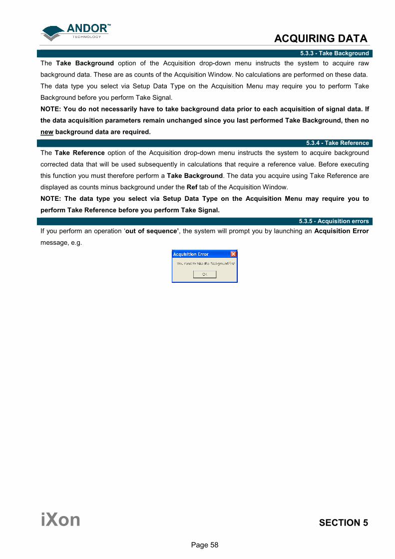
5.3.5 - Acquisition errors
If you perform an operation ‘out of sequence’, the system will prompt you by launching an Acquisition Error
message, e.g.
ACQUIRING DATA
iXon SECTION 5
Page 59
5.4 - ACQUISITION MODES & TIMINGS
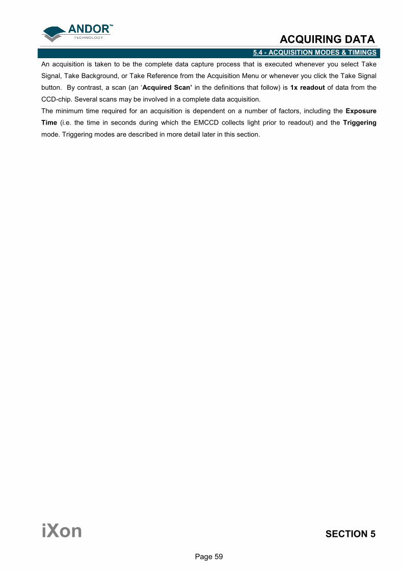
An acquisition is taken to be the complete data capture process that is executed whenever you select Take
Signal, Take Background, or Take Reference from the Acquisition Menu or whenever you click the Take Signal
button. By contrast, a scan (an ‘Acquired Scan’ in the definitions that follow) is 1x readout of data from the
CCD-chip. Several scans may be involved in a complete data acquisition.
The minimum time required for an acquisition is dependent on a number of factors, including the Exposure
Time (i.e. the time in seconds during which the EMCCD collects light prior to readout) and the Triggering
mode. Triggering modes are described in more detail later in this section.
ACQUIRING DATA
iXon SECTION 5
Page 60
5.4.1 - Single
Single scan is the simplest acquisition mode, in which the system performs one scan of the CCD.
NOTE: Should you attempt to enter too low a value, the system will default to a minimum Exposure
Time.
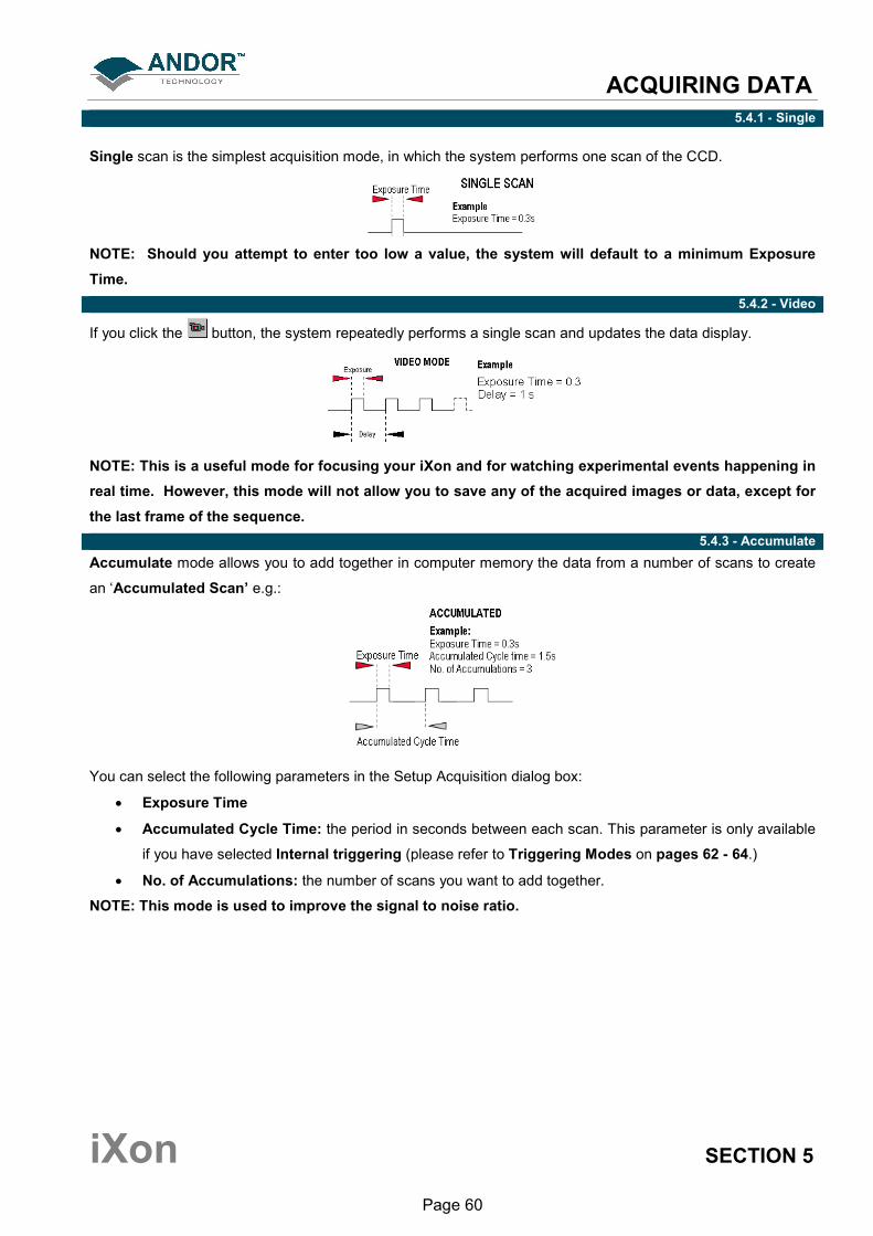
5.4.2 - Video
If you click the button, the system repeatedly performs a single scan and updates the data display.
NOTE: This is a useful mode for focusing your iXon and for watching experimental events happening in
real time. However, this mode will not allow you to save any of the acquired images or data, except for
the last frame of the sequence.
5.4.3 - Accumulate
Accumulate mode allows you to add together in computer memory the data from a number of scans to create
an ‘Accumulated Scan’ e.g.:
You can select the following parameters in the Setup Acquisition dialog box:
• Exposure Time
• Accumulated Cycle Time: the period in seconds between each scan. This parameter is only available
if you have selected Internal triggering (please refer to Triggering Modes on pages 62 - 64.)
• No. of Accumulations: the number of scans you want to add together.
NOTE: This mode is used to improve the signal to noise ratio.

ACQUIRING DATA
iXon SECTION 5
Page 61
5.4.4 - Kinetic Series
In the Setup Acquisition dialog box you can key in the following parameters:
• Exposure Time
• Kinetic Cycle Time: the time between the start and finish of each kinetic scan.
• Number in Kinetic Series: the number of scans taken in the kinetic series.
NOTE: This mode is particularly well suited to recording the temporal evolution of a process.
5.4.4.1 - Frame Rates
The Kinetic Cycle Time can also be act as a useful guide to the Frame Rate your camera is operating at.
Depending on the Acquisition parameters you set, i.e. Vertical Shift Speed, Binning or Sub Image Patterns,
Cycle Time and whether External Trigger is being used, the Kinetic Cycle Dialog box will display a Hz figure.
As a guide 1 Hz equals 1 frame per second.
If External trigger is selected the Kinetic Cycle dialog box will indicate the maximum achievable frame rate.

ACQUIRING DATA
iXon SECTION 5
Page 62
5.5 - TRIGGERING MODES
The Triggering modes are selected from a drop-down list on the Setup Acquisition dialog box:
The modes you can select are as follows:
• Internal
• External
• Fast External
• External Start

ACQUIRING DATA
iXon SECTION 5
Page 63
5.5.1 - Internal
In Internal mode, once you issue a data acquisition command, the system determines when data acquisition
begins. You can use Internal mode when you are able to send a trigger signal or ‘Fire Pulse’ to a short-
duration, pulsed source (e.g. a laser). In this case starting data acquisition also signals the pulsed source to fire.
The Fire Pulse is fed from the Fire SMB connector on the detector.
Internal Trigger Mode is also used with ‘Continuous Wave’ (CW) sources (e.g. an ordinary room light) where
incoming data, for the purposes of your observation, are steady and unbroken. This means that acquisitions
can be taken at will.
IMPORTANT NOTE ON EXTERNAL TRIGGERING MODES: If you have a shutter connected, and are
using External Triggering, you must ensure that the shutter is open before the optical signal you want
to measure occurs.
5.5.2 - External
In External mode once you issue a data acquisition command, data will not be acquired until your system has
received an External Trigger signal generated by an external device (e.g. a laser). The External Triggering
signal is fed to the Ext Trig SMB connector on the rear of the detector.
5.5.3 - Fast External
Normally, when using External Trigger the system will only enable the triggering of the system after a complete
Keep Clean Cycle has been performed. This is to ensure that the CCD is always in the same known state
before it is triggered. This is particularly important when the system is in Accumulation or Kinetics mode.
In cases were repetition rate is paramount, and slight variation in the base background level is less important, it
is possible to remove this restriction by using Fast External triggering.
NOTES:
1. The Keep Clean process is continuous on the iXon and any delay is negligible.
2. If you need Maximum Repetition Rate, have a shutter connected and are using Fast External
triggering, you must again ensure that the shutter is open before the optical signal you want to
measure occurs.
5.5.4 - External Start
With External Start triggering, once you issue a data acquisition command, data will not be acquired until your
system has received an external trigger signal generated by an external device. The system will then continue
to acquire data based on user options set within the Acquisition Dialog. This means that an External Start
Trigger could be used to commence acquisition of a Kinetic series, but with the parameters of that series being
controlled by internal software options. The External Start trigger signal is fed to the camera head via the Ext
Trig SMB on the back of the camera.

ACQUIRING DATA
iXon SECTION 5
Page 64
5.6 - SELECTING TRIGGERING MODE
The flowchart below may help you decide whether you should use Internal, External, External Start or Fast
External triggering.
ACQUIRING DATA
iXon SECTION 5
Page 65
5.7- READOUT MODES
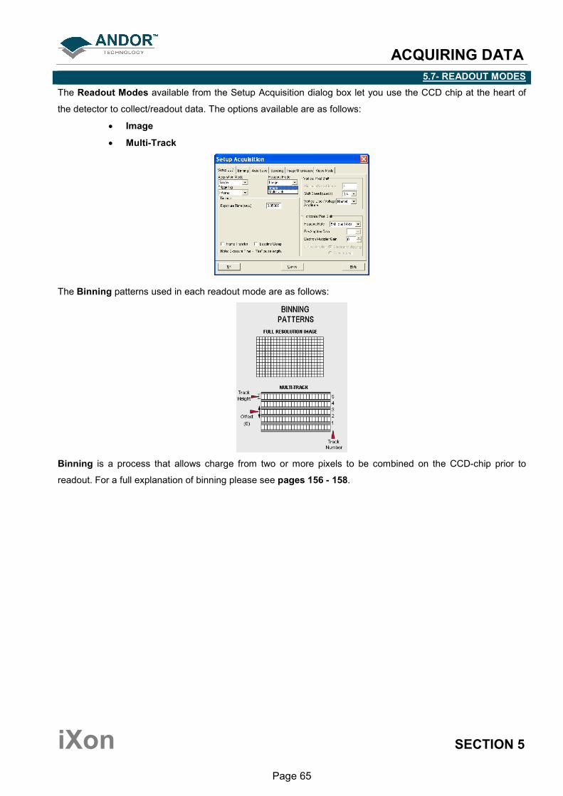
The Readout Modes available from the Setup Acquisition dialog box let you use the CCD chip at the heart of
the detector to collect/readout data. The options available are as follows:
• Image
• Multi-Track
The Binning patterns used in each readout mode are as follows:
Binning is a process that allows charge from two or more pixels to be combined on the CCD-chip prior to
readout. For a full explanation of binning please see pages 156 - 158.
ACQUIRING DATA
iXon SECTION 5
Page 66
5.7.1 – Image mode
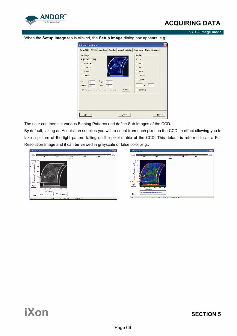
When the Setup Image tab is clicked, the Setup Image dialog box appears, e.g.:
The user can then set various Binning Patterns and define Sub Images of the CCD.
By default, taking an Acquisition supplies you with a count from each pixel on the CCD, in effect allowing you to
take a picture of the light pattern falling on the pixel matrix of the CCD. This default is referred to as a Full
Resolution Image and it can be viewed in grayscale or false color ,e.g.:

ACQUIRING DATA
iXon SECTION 5
Page 67
5.7.1.1 - Sub Image
For the purpose of initial focusing and alignment of the camera, or to increase the readout speed, you may use
the software to select a Sub Image of the chip.
To select Sub Image mode, click on the button. When the iXon is running in Sub Image mode, only data
from the selected pixels will be readout, data from the remaining pixels will be discarded. To read out data from
a selected area (or Sub Image) of the CCD use the radio buttons to select the resolution, which you require,
e.g.:
The software offers a choice of three defined sub images:
• 256 x 256 pixels
• 128 x 128 pixels
• 64 x 64 pixels.
There is also an option for you to define a Custom Sub Image. This function allows you to set the Sub Image to
any size and location on the CCD chip. To define a Custom Sub Image tick the Custom button, then use the
co-ordinate entry dialogue boxes to select the size and location of your sub image.
5.7.1.1.1 - Draw
In addition to the previous methods of defining a Sub Image on the CCD, you can also use the Draw Option to
select the size and location of your Sub Image. In order to use the Draw Option, you must first acquire a full
resolution image. This will be the template on which you will draw your Sub Image.
Click on the button then use the Draw tool to select the size and position of your Sub Image by dragging
rulers form the X and Y-axis. Alternatively, a Sub Image can be drawn on the template by positioning your
cursor on the image, and dragging out the shape of the Sub Image area you require.
5.7.1.1.2 - Superpixels
As well as selecting a Sub Image of the CCD, you can also use a system of pixel charge aggregation, known as
Binning, to create Superpixels. Superpixels consist of two or more individual pixels that are binned and read
out as one large pixel. The CCD, or your selected sub-area, then becomes a matrix of superpixels.
ACQUIRING DATA
iXon SECTION 5
Page 68
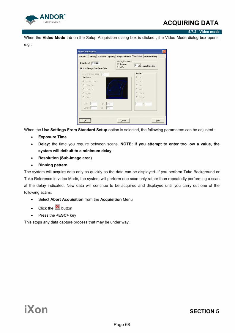
5.7.2 - Video mode
When the Video Mode tab on the Setup Acquisition dialog box is clicked , the Video Mode dialog box opens,
e.g.:
When the Use Settings From Standard Setup option is selected, the following parameters can be adjusted :
• Exposure Time
• Delay: the time you require between scans. NOTE: If you attempt to enter too low a value, the
system will default to a minimum delay.
• Resolution (Sub-image area)
• Binning pattern
The system will acquire data only as quickly as the data can be displayed. If you perform Take Background or
Take Reference in video Mode, the system will perform one scan only rather than repeatedly performing a scan
at the delay indicated. New data will continue to be acquired and displayed until you carry out one of the
following actins:
• Select Abort Acquisition from the Acquisition Menu
• Click the button
• Press the <ESC> key
This stops any data capture process that may be under way.
ACQUIRING DATA
iXon SECTION 5
Page 69
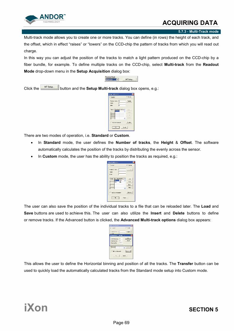
5.7.3 - Multi-Track mode
Multi-track mode allows you to create one or more tracks. You can define (in rows) the height of each track, and
the offset, which in effect “raises” or “lowers” on the CCD-chip the pattern of tracks from which you will read out
charge.
In this way you can adjust the position of the tracks to match a light pattern produced on the CCD-chip by a
fiber bundle, for example. To define multiple tracks on the CCD-chip, select Multi-track from the Readout
Mode drop-down menu in the Setup Acquisition dialog box:
Click the button and the Setup Multi-track dialog box opens, e.g.:
There are two modes of operation, i.e. Standard or Custom.
• In Standard mode, the user defines the Number of tracks, the Height & Offset. The software
automatically calculates the position of the tracks by distributing the evenly across the sensor.
• In Custom mode, the user has the ability to position the tracks as required, e.g.:
The user can also save the position of the individual tracks to a file that can be reloaded later. The Load and
Save buttons are used to achieve this. The user can also utilize the Insert and Delete buttons to define
or remove tracks. If the Advanced button is clicked, the Advanced Multi-track options dialog box appears:
This allows the user to define the Horizontal binning and position of all the tracks. The Transfer button can be
used to quickly load the automatically calculated tracks from the Standard mode setup into Custom mode.
ACQUIRING DATA
iXon SECTION 5
Page 70
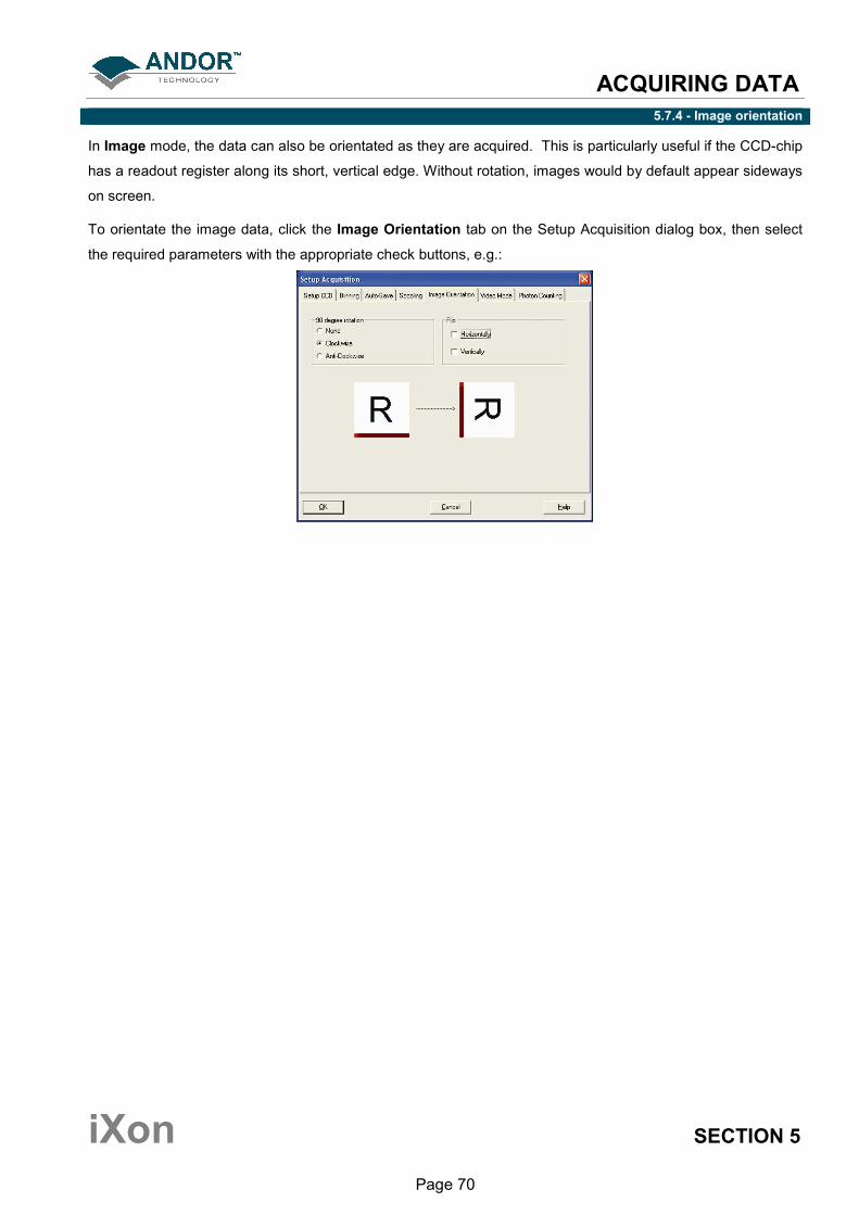
5.7.4 - Image orientation
In Image mode, the data can also be orientated as they are acquired. This is particularly useful if the CCD-chip
has a readout register along its short, vertical edge. Without rotation, images would by default appear sideways
on screen.
To orientate the image data, click the Image Orientation tab on the Setup Acquisition dialog box, then select
the required parameters with the appropriate check buttons, e.g.:
ACQUIRING DATA
iXon SECTION 5
Page 71
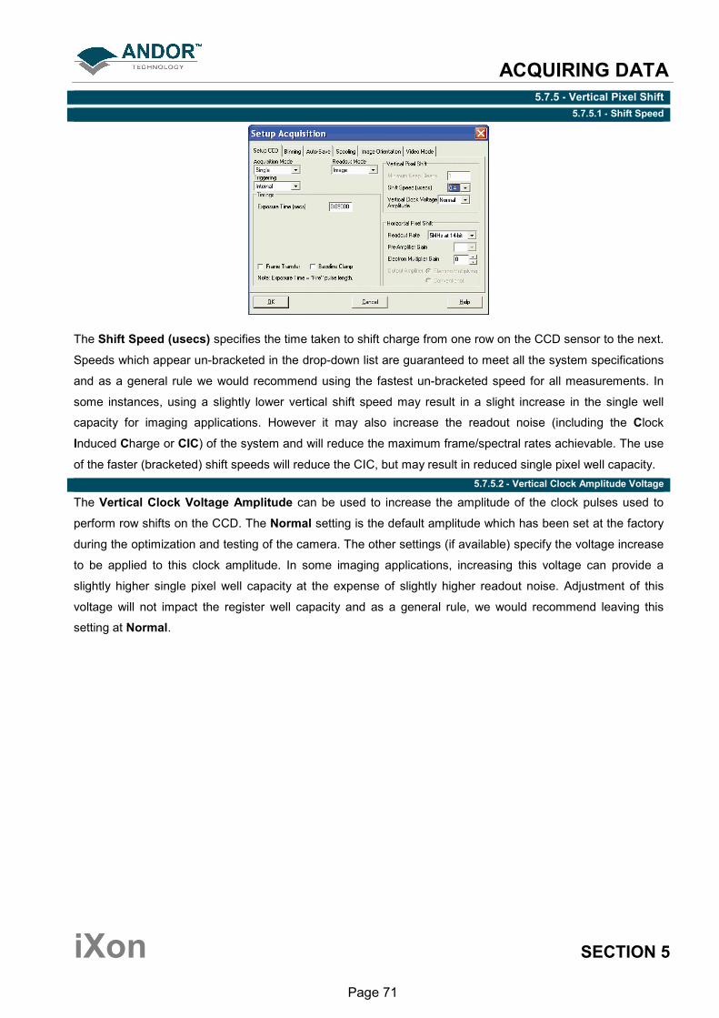
5.7.5 - Vertical Pixel Shift 5.7.5.1 - Shift Speed
The Shift Speed (usecs) specifies the time taken to shift charge from one row on the CCD sensor to the next.
Speeds which appear un-bracketed in the drop-down list are guaranteed to meet all the system specifications
and as a general rule we would recommend using the fastest un-bracketed speed for all measurements. In
some instances, using a slightly lower vertical shift speed may result in a slight increase in the single well
capacity for imaging applications. However it may also increase the readout noise (including the Clock
Induced Charge or CIC) of the system and will reduce the maximum frame/spectral rates achievable. The use
of the faster (bracketed) shift speeds will reduce the CIC, but may result in reduced single pixel well capacity.
5.7.5.2 - Vertical Clock Amplitude Voltage
The Vertical Clock Voltage Amplitude can be used to increase the amplitude of the clock pulses used to
perform row shifts on the CCD. The Normal setting is the default amplitude which has been set at the factory
during the optimization and testing of the camera. The other settings (if available) specify the voltage increase
to be applied to this clock amplitude. In some imaging applications, increasing this voltage can provide a
slightly higher single pixel well capacity at the expense of slightly higher readout noise. Adjustment of this
voltage will not impact the register well capacity and as a general rule, we would recommend leaving this
setting at Normal.

ACQUIRING DATA
iXon SECTION 5
Page 72
5.7.6 - Horizontal Pixel Shift
5.7.6.1- Readout Rate
The Horizontal Pixel Shift Readout Rate defines the rate at which pixels are read from the shift register. The
faster the Horizontal Readout Rate the higher the frame rate that can be achieved. Slower readout rates will
generate less noise in the data as it is read out. The rate can be selected from a drop-down list on the Setup
Acquisition dialog box, e.g.:
5.7.6.2 - Pre-Amplifier Gain
The Pre-Amplifier gain determines the amount of gain applied to the video signal emerging from the CCD and
allows the user to control the sensitivity of the camera system. On all iXon cameras there are three options
available i.e. x1, x2 or x4. These normalized gain settings will correspond to system sensitivities specified on
the performance sheets (in terms of electrons per A/D count) which accompany the system.
Selecting higher pre-amplifier gain values (i.e. x2 or x4) will increase the sensitivity of the camera (i.e. fewer
electrons will be required to produce one A/D count) and provide the lowest readout noise performance.
However this may result in the A/D converter saturating before the single pixel / register capacity of the CCD
sensor is reached.
5.7.6.3 - Output Amplifier
For the DU-888 & DU-897 models, the output amplifier radio button allows the user to select though which on-
chip amplifier the data will emerge through. The various options available (if any) will vary depending on the
CCD sensor type incorporated in the camera system. The user can select either the Electron Multiplying (EM)
or Conventional (non-EM) output amplifier
ACQUIRING DATA
iXon SECTION 5
Page 73
5.8 - TIMING PARAMETER
Depending on which combination of Acquisition, Readout & Triggering modes is selected, various timing
parameters are available as follow:
• Exposure Time (secs)
• No. of Accumulations
• Accumulation Cycle Time (secs)
• Cosmic Ray Removal
• Kinetic Series Length
• Kinetic Cycle Time (secs)

ACQUIRING DATA
iXon SECTION 5
Page 74
5.9 - SHUTTER
A shutter can be used to take a reference or background if Full Vertical Binning is selected. For either Multi-
Track or Image mode, the shutter is required to avoid unnecessary signals/light falling on the CCD during the
readout process; otherwise the image will be smeared. When the Shutter Control option is selected from the
Hardware drop-down-menu, the Shutter Control dialog box opens e.g.:
You can use this to indicate when and how a hardware shutter should be used. With a CCD, the shutter is
used for background shuttering. Certain settings (e.g. Permanently OPEN & Permanently CLOSED) take
effect as soon as you close the Shutter Control dialog box. Other settings will be applied whenever you acquire
data.
ACQUIRING DATA
iXon SECTION 5
Page 75
• Fully Auto is the simplest shutter mode, as it leaves all shuttering decisions to the system. When you
perform Take Signal the shutter opens for the duration of the Exposure Time you have entered in the
Setup Acquisition dialog box. NOTE: This option will automatically provide suitable shuttering for
the majority of data acquisitions. The shutter will be closed for background data acquisitions
and will be opened for all other data acquisitions.
• If CLOSED for background mode is selected, any shutter driven from the Shutter output will be
closed as you perform Take Background. If you want the shutter to be open so that the Take
Background function records genuine optical background data, deselect the option. NOTE:
Usually a background scan is used to subtract the dark signal and the Fixed Pattern Noise
(FPN) of the sensor. For this reason the background scan is usually performed in darkness. A
shutter may be used to stop light entering the spectrograph or other imaging system. Strictly
speaking though, the background acquisition may be regarded as comprising all light with the
single exception of the source. Thus, when you are working with a pulsed or independently
shuttered source, it may be appropriate to have the mode deselected.
• In Permanently OPEN mode, the shutter will be open before, during and after any data acquisition.
• Permanently CLOSED mode can be useful if you want to take a series of acquisitions in darkness and
do not require the shutter to open between acquisitions. You might, for example, wish to capture a
sequence of background values. The shutter remains closed before, during and after any data
acquisition.
The TTL (Transistor-Transistor Logic) buttons, TTL Low & TTL High, let you instruct the system as to how it
should control the opening and closing of the shutter.
If you select TTL Low, the system will cause the output voltage from the iXon to go ‘low’ to open the
shutter.
If you select TTL High, the system will cause the output voltage from the iXon to go ‘high’ to open the
shutter.
The documentation supplied by the shutter manufacturer will show whether your shutter opens at a high or a
low TTL level.
NOTES:
1. The iXon contains a Frame Transfer CCD device, so a shutter may not be required for most
applications. If a shutter is fitted but not required for the experiment, then set it to permanently
open, and Time to 0. This will allow the system to operate at its optimum rate. If a Background is
required then close the shutter using Permanently CLOSED, take the Background and reopen.
2. The shutter pulse is not capable of driving a shutter. It is only a 5V pulse designed to trigger
TTL & CMOS compatible shutter drivers. Also there is no shutter pulse during the Take Signal
and Take Reference data acquisitions.
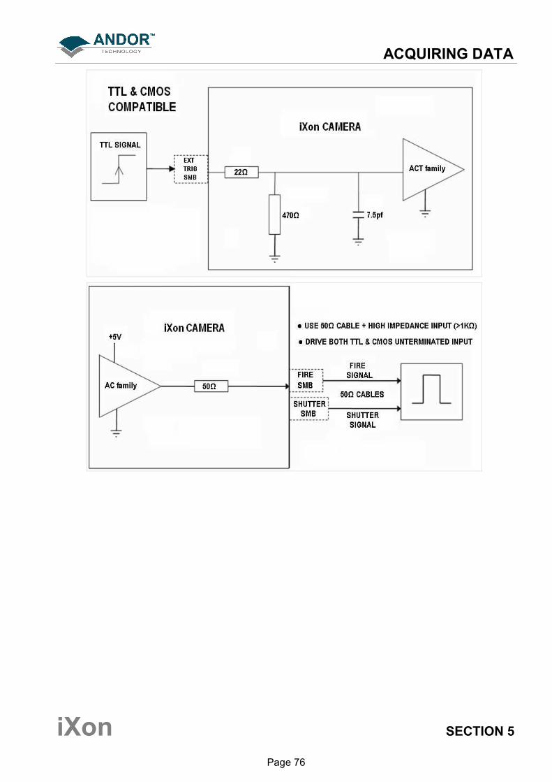
ACQUIRING DATA
iXon SECTION 5
Page 76
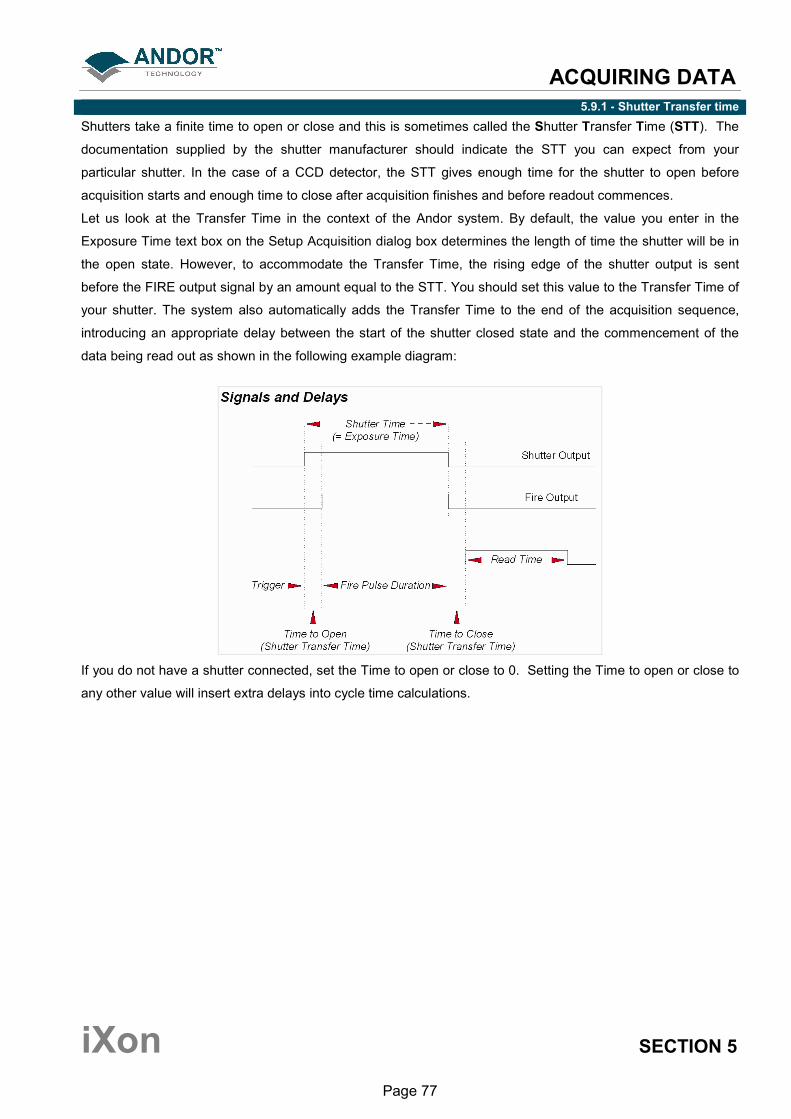
ACQUIRING DATA
iXon SECTION 5
Page 77
5.9.1 - Shutter Transfer time
Shutters take a finite time to open or close and this is sometimes called the Shutter Transfer Time (STT). The
documentation supplied by the shutter manufacturer should indicate the STT you can expect from your
particular shutter. In the case of a CCD detector, the STT gives enough time for the shutter to open before
acquisition starts and enough time to close after acquisition finishes and before readout commences.
Let us look at the Transfer Time in the context of the Andor system. By default, the value you enter in the
Exposure Time text box on the Setup Acquisition dialog box determines the length of time the shutter will be in
the open state. However, to accommodate the Transfer Time, the rising edge of the shutter output is sent
before the FIRE output signal by an amount equal to the STT. You should set this value to the Transfer Time of
your shutter. The system also automatically adds the Transfer Time to the end of the acquisition sequence,
introducing an appropriate delay between the start of the shutter closed state and the commencement of the
data being read out as shown in the following example diagram:
If you do not have a shutter connected, set the Time to open or close to 0. Setting the Time to open or close to
any other value will insert extra delays into cycle time calculations.
ACQUIRING DATA
iXon SECTION 5
Page 78
5.9.2 - Accumulate Cycle Time & No. of Accumulations
If you have selected Accumulate or Kinetic as the acquisition mode, with Internal triggering, you can also
select the Accumulation Cycle Time and No. of Accumulations.
• The Accumulation Cycle Time is the period in seconds between each of a number of scans, whose data
are to be added together in computer memory to form an Accumulated Scan.
• The Number of Accumulations indicates the number of scans you want to add together.
5.9.3 - Kinetic Series & Kinetic Cycle Lengths
When Kinetic is selected as the acquisition mode, with Internal triggering you can also select the Kinetic
Series Length and Kinetic Cycle Length (secs).
• The Kinetic Series Length is the number of scans you require in your series
• The Kinetic Cycle Length is the interval (in seconds) at which each scan (or accumulated scan) in your
series begins.

ACQUIRING DATA
iXon SECTION 5
Page 79
5.9.4 - Fast Kinetics
Fast Kinetics allows exposure times on a microsecond timescale. Use Fast Kinetics when you need an
exposure time that is smaller than the minimum Kinetic Cycle Time in a standard Kinetic Series.
In Fast Kinetics the image to be recorded is imaged across a certain section of the CCD. The non-illuminated
part of the CCD is used for storage of image before readout. You must ensure that light does not fall on this
storage part of the CCD by using, for example, an imaging spectrograph. By way of explanation, take the
example of an illuminated sub-area of height 8 rows. A CW spectrum is imaged along this sub-area and the
resulting image is then shifted down 8 rows into the non-illuminated area, thus sampling the image in time. In
this way the image is temporarily stored on the CCD itself, rather than in the computer. The process is repeated
until the frame of the CCD is filled with time-sampled images or until the number of images you have specified
for your series has been acquired. Next each image is transferred into the shift register in turn, and read out in
the normal way. With a CCD-chip of height 512 pixels and a sub-area height of 8 rows, 63 discrete images can
be stored on the CCD (not 64 images, since the top 8 rows of the CCD constitute the illuminated sub-area,
which cannot be used for storage.) From the Setup Acquisition dialog box, you can change the following
parameters:
• Exposure Time: the Exposure Time also represents the cycle time of the Fast Kinetics series. There is
no separate parameter for a Fast Kinetics cycle time
• Sub Area Height in rows
• Number in Series: the number of time-sampled images you want to acquire
• Binning of the images
• Offset of the active area from the bottom of the detector can also be specified

ACQUIRING DATA
iXon SECTION 5
Page 80
5.9.4.1 - Readout Mode & Fast Kinetics
The data from each of the spectra in the Fast Kinetics series is stored as an image. Select Image from the
Readout Mode drop down list on the Setup Acquisition Window. Fast kinetics is not available in multi-track
mode. With Fast Kinetics you may use the following Trigger Modes: Internal, External, Fast External and
External Start.
• In Internal Trigger mode, the system determines when the acquisition begins, and then uses the
acquisition settings defined by the user. This mode is equivalent to the internal triggering mode for
Single Scan etc.
• In External Trigger mode, a trigger pulse is required to start each scan in the series. The rising edge of
the trigger starts the exposure time. After the exposure time has elapsed, the number of rows, as
specified by the user, are vertically shifted. The system then waits for the next trigger to start the next
scan. As there is no keep clean cycle running while waiting for the external trigger the "real "exposure
time is the time between each trigger. A consequence of this is that if your experiment has a constant
background signal but your trigger period is not fixed you may see different background levels in your
signal.
• In External Start Trigger mode, data will not be acquired until the system receives an initial external
trigger signal from an external device, like a laser. From that point on, the system alone determines
when data are acquired based on the user settings, as in the case of Internal Trigger. As the system
changes from an external trigger mode to internal trigger mode on receipt of the initial trigger signal the
exposure time of the first scan in the series will not be the same as the subsequent scans. The
exposure time is defined as the time between vertical shifts.

ACQUIRING DATA
iXon SECTION 5
Page 81
5.10 - FILE INFORMATION
Details of the Acquisition selection can be viewed by clicking the button on the Main Window which opens
the Information dialog box (you can enter your own notes in the Comments box):
The table below details the type of information contained in the dialog box.
Table 9: Information dialog box
Filename
The filename associated with the active Data Window.
If the data has not yet been saved this will default to
Acquisition Date and time The date & time at which the acquisition was made.
Temperature (C) The temperature to which the detector had been cooled.
Model The model number of the detector.
Data Type Data Type – Counts, % Transmittance, etc.
Acquisition Mode Single, Accumulate or Kinetic
Trigger Mode Internal, External or Fast External
Exposure Time (secs) “Fire” pulse length
Delay (secs) Value in microseconds
Horizontal Binning Always = 1
Vertical Binning Minimum = 1, Maximum = 256
Horizontally flipped True or False
Vertically flipped True or False
Clockwise rotation True or False
Anti-clockwise rotation True or False
Pixel Readout Time (µsecs) Value in microseconds
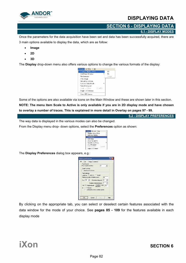
DISPLAYING DATA
iXon SECTION 6
Page 82
SECTION 6 - DISPLAYING DATA 6.1 - DISPLAY MODES
Once the parameters for the data acquisition have been set and data has been successfully acquired, there are
3 main options available to display the data, which are as follow:
• Image
• 2D
• 3D
The Display drop-down menu also offers various options to change the various formats of the display:
Some of the options are also available via icons on the Main Window and these are shown later in this section.
NOTE: The menu item Scale to Active is only available if you are in 2D display mode and have chosen
to overlay a number of traces. This is explained in more detail in Overlay on pages 97 - 99.
6.2 - DISPLAY PREFERENCES
The way data is displayed in the various modes can also be changed.
From the Display menu drop- down options, select the Preferences option as shown:
The Display Preferences dialog box appears, e.g.:
By clicking on the appropriate tab, you can select or deselect certain features associated with the
data window for the mode of your choice. See pages 85 - 109 for the features available in each
display mode
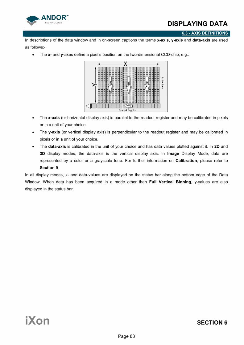
DISPLAYING DATA
iXon SECTION 6
Page 83
6.3 - AXIS DEFINITIONS
In descriptions of the data window and in on-screen captions the terms x-axis, y-axis and data-axis are used
as follows:-
• The x- and y-axes define a pixel’s position on the two-dimensional CCD-chip, e.g.:
• The x-axis (or horizontal display axis) is parallel to the readout register and may be calibrated in pixels
or in a unit of your choice.
• The y-axis (or vertical display axis) is perpendicular to the readout register and may be calibrated in
pixels or in a unit of your choice.
• The data-axis is calibrated in the unit of your choice and has data values plotted against it. In 2D and
3D display modes, the data-axis is the vertical display axis. In Image Display Mode, data are
represented by a color or a grayscale tone. For further information on Calibration, please refer to
Section 9.
In all display modes, x- and data-values are displayed on the status bar along the bottom edge of the Data
Window. When data has been acquired in a mode other than Full Vertical Binning, y-values are also
displayed in the status bar.
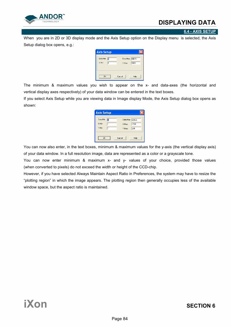
DISPLAYING DATA
iXon SECTION 6
Page 84
6.4 - AXIS SETUP
When you are in 2D or 3D display mode and the Axis Setup option on the Display menu is selected, the Axis
Setup dialog box opens, e.g.:
The minimum & maximum values you wish to appear on the x- and data-axes (the horizontal and
vertical display axes respectively) of your data window can be entered in the text boxes.
If you select Axis Setup while you are viewing data in Image display Mode, the Axis Setup dialog box opens as
shown:
You can now also enter, in the text boxes, minimum & maximum values for the y-axis (the vertical display axis)
of your data window. In a full resolution image, data are represented as a color or a grayscale tone.
You can now enter minimum & maximum x- and y- values of your choice, provided those values
(when converted to pixels) do not exceed the width or height of the CCD-chip.
However, if you have selected Always Maintain Aspect Ratio in Preferences, the system may have to resize the
“plotting region” in which the image appears. The plotting region then generally occupies less of the available
window space, but the aspect ratio is maintained.
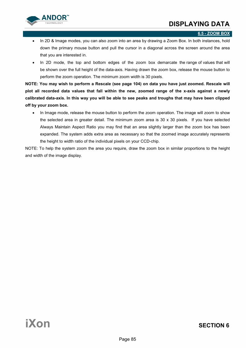
DISPLAYING DATA
iXon SECTION 6
Page 85
6.5 - ZOOM BOX
• In 2D & Image modes, you can also zoom into an area by drawing a Zoom Box. In both instances, hold
down the primary mouse button and pull the cursor in a diagonal across the screen around the area
that you are interested in.
• In 2D mode, the top and bottom edges of the zoom box demarcate the range of values that will
be shown over the full height of the data-axis. Having drawn the zoom box, release the mouse button to
perform the zoom operation. The minimum zoom width is 30 pixels.
NOTE: You may wish to perform a Rescale (see page 104) on data you have just zoomed. Rescale will
plot all recorded data values that fall within the new, zoomed range of the x-axis against a newly
calibrated data-axis. In this way you will be able to see peaks and troughs that may have been clipped
off by your zoom box.
• In Image mode, release the mouse button to perform the zoom operation. The image will zoom to show
the selected area in greater detail. The minimum zoom area is 30 x 30 pixels. If you have selected
Always Maintain Aspect Ratio you may find that an area slightly larger than the zoom box has been
expanded. The system adds extra area as necessary so that the zoomed image accurately represents
the height to width ratio of the individual pixels on your CCD-chip.
NOTE: To help the system zoom the area you require, draw the zoom box in similar proportions to the height
and width of the image display.
DISPLAYING DATA
iXon SECTION 6
Page 86
6.6 - ZOOMING & SCROLLING
The following functions are available in data windows whilst in 2D & 3D Display modes:
• Zoom in
• Zoom out
• Scroll
6.6.1 - Zoom In & Zoom Out
On a data window in 2D or 3D display mode, pairs of Zoom In; and Zoom Out; buttons are
provided on both the x- and data-axes of the trace. These buttons allow you to stretch or shrink the scale (to
cover a smaller or larger range) on either the x- or data-axis, creating the effect of zooming in or zooming out in
either the vertical or horizontal dimension of the display.
6.6.2 - Scrolling
If you have stretched a scale by zooming, you can slide the scale to cover a different range and the display will
scroll in synchronization with the moving scale. Place the cursor arrow over the scale so that it changes to a
finger flanked by arrows. Now depressing the primary mouse button allows you to “slide” the scale up and down
(or left and right) and scroll the display.
If you place the finger cursor at either end of an axis you will notice that a single arrow appears beside
it, indicating the direction in which the scale will slide automatically when you depress the primary mouse button
the display “fast scrolls” accordingly.
6.6.3 - Reset
Clicking the button when a Data Window is open, returns the displayed data to its original configuration,
thus undoing any adjustment to scale that you may have performed in accordance with the descriptions given in
Zooming In, Zooming Out, Scrolling and Rescale (see page 104 for more information on rescaling). Reset is
available for all display modes.
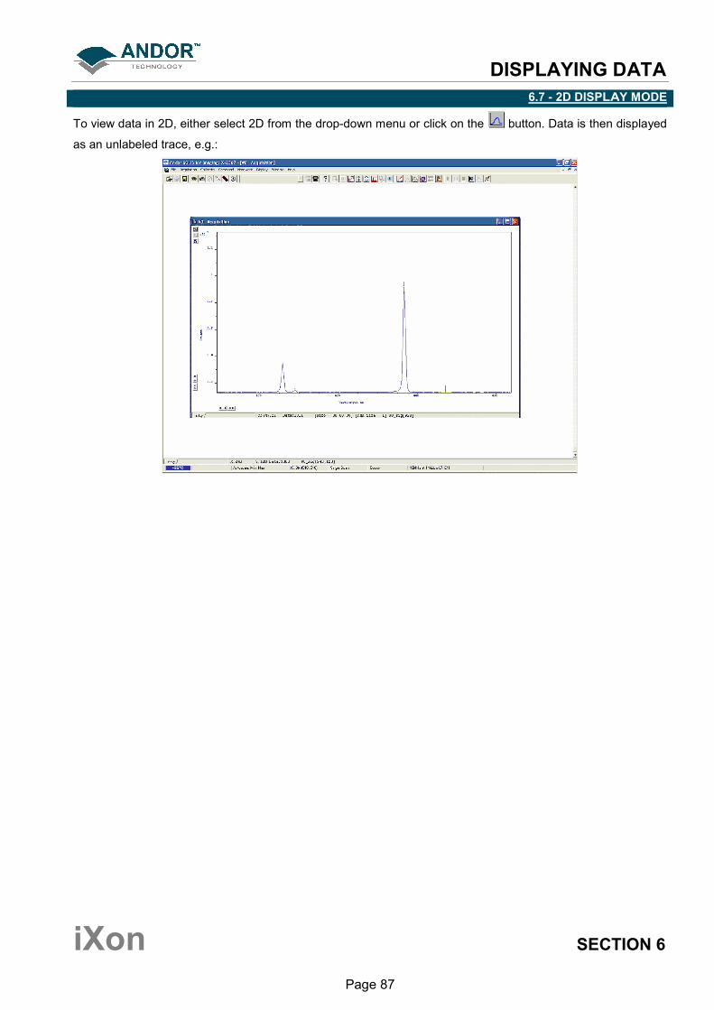
DISPLAYING DATA
iXon SECTION 6
Page 87
6.7 - 2D DISPLAY MODE
To view data in 2D, either select 2D from the drop-down menu or click on the button. Data is then displayed
as an unlabeled trace, e.g.:

DISPLAYING DATA
iXon SECTION 6
Page 88
6.7.1 - 2D display mode preferences
The following options are available to view peaks when in 2D Display mode:
6.7.1.1 - Peak Search
6.7.1.1.1 - Peak Search Sensitivity
The Peak Search Sensitivity option Determines the manner in which the cursor moves between peaks/troughs
when you key in Ctrl + Right Arrow or Ctrl + Left Arrow.
• A low sensitivity (e.g. 1) means the system will find the most prominent peaks or troughs
• A high sensitivity (e.g. 5) means less obvious peaks or troughs will be found
NOTE: This parameter relates only to Peak Search, not to Peak Labeling.
6.7.1.2 - Peak Labeling
6.7.1.2.1 - Labels on Peaks or Troughs
Lets you choose whether to mark the highest points (peaks) or lowest points (troughs) on the trace.
6.7.1.2.2 - Maximum Number of Labeled Peaks
Causes only the highest peaks or lowest troughs, up to the total number of peaks/troughs indicated, to
be labeled automatically.
6.7.1.2.3 - Format Labels
Size, Orientation & Number of Decimal Places lets you format the peak labels
For Orientation, 0° is horizontal; 90° vertical. You can have up to 4 decimal places in the label
6.7.1.2.4 - Weighted Peak
Weighted Peak in combination with a Weighted Range (centered on the highest/lowest positioned pixel) lets the
system calculate and label a weighted mean to represent the peak or trough. NOTE: This feature works best on
peaks or troughs which are symmetrical about the highest/lowest point.
6.7.1.3 - Pixel Peak
The system can label the Pixel Peak (the highest/lowest positioned pixel).
6.7.1.3.1 - Label Peaks in all Overlaid Spectra
You can also choose whether to Label peaks in all overlaid spectra or to have peaks labeled only on the active
trace. See Overlay on pages 90 - 94.
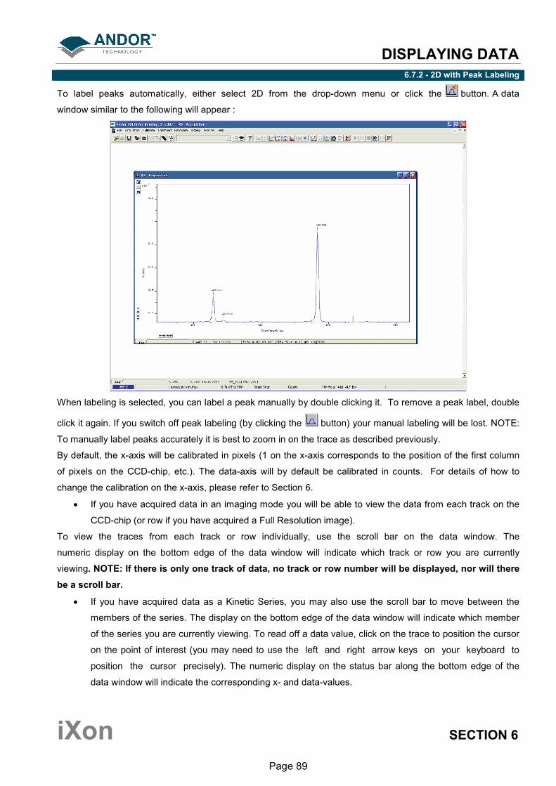
DISPLAYING DATA
iXon SECTION 6
Page 89
6.7.2 - 2D with Peak Labeling
To label peaks automatically, either select 2D from the drop-down menu or click the button. A data
window similar to the following will appear :
When labeling is selected, you can label a peak manually by double clicking it. To remove a peak label, double
click it again. If you switch off peak labeling (by clicking the button) your manual labeling will be lost. NOTE:
To manually label peaks accurately it is best to zoom in on the trace as described previously.
By default, the x-axis will be calibrated in pixels (1 on the x-axis corresponds to the position of the first column
of pixels on the CCD-chip, etc.). The data-axis will by default be calibrated in counts. For details of how to
change the calibration on the x-axis, please refer to Section 6.
• If you have acquired data in an imaging mode you will be able to view the data from each track on the
CCD-chip (or row if you have acquired a Full Resolution image).
To view the traces from each track or row individually, use the scroll bar on the data window. The
numeric display on the bottom edge of the data window will indicate which track or row you are currently
viewing. NOTE: If there is only one track of data, no track or row number will be displayed, nor will there
be a scroll bar.
• If you have acquired data as a Kinetic Series, you may also use the scroll bar to move between the
members of the series. The display on the bottom edge of the data window will indicate which member
of the series you are currently viewing. To read off a data value, click on the trace to position the cursor
on the point of interest (you may need to use the left and right arrow keys on your keyboard to
position the cursor precisely). The numeric display on the status bar along the bottom edge of the
data window will indicate the corresponding x- and data-values.
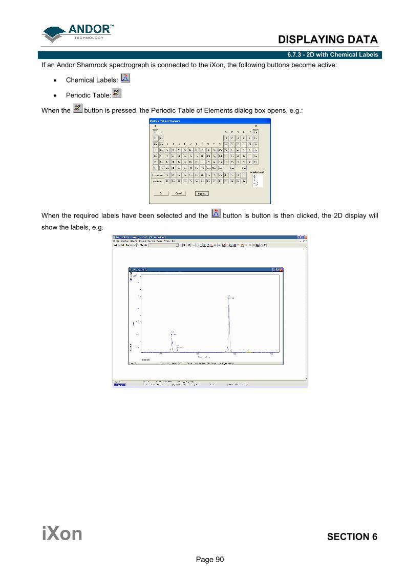
DISPLAYING DATA
iXon SECTION 6
Page 90
6.7.3 - 2D with Chemical Labels
If an Andor Shamrock spectrograph is connected to the iXon, the following buttons become active:
• Chemical Labels:
• Periodic Table:
When the button is pressed, the Periodic Table of Elements dialog box opens, e.g.:
When the required labels have been selected and the button is button is then clicked, the 2D display will
show the labels, e.g.
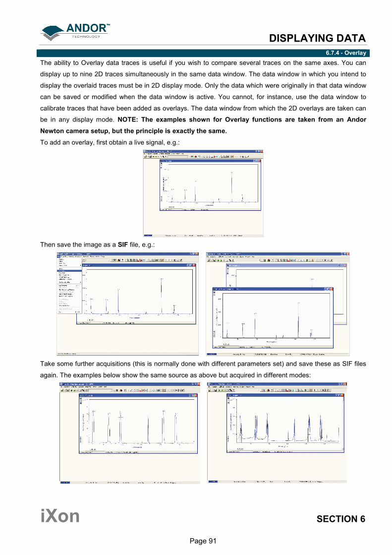
DISPLAYING DATA
iXon SECTION 6
Page 91
6.7.4 - Overlay
The ability to Overlay data traces is useful if you wish to compare several traces on the same axes. You can
display up to nine 2D traces simultaneously in the same data window. The data window in which you intend to
display the overlaid traces must be in 2D display mode. Only the data which were originally in that data window
can be saved or modified when the data window is active. You cannot, for instance, use the data window to
calibrate traces that have been added as overlays. The data window from which the 2D overlays are taken can
be in any display mode. NOTE: The examples shown for Overlay functions are taken from an Andor
Newton camera setup, but the principle is exactly the same.
To add an overlay, first obtain a live signal, e.g.:
Then save the image as a SIF file, e.g.:
Take some further acquisitions (this is normally done with different parameters set) and save these as SIF files
again. The examples below show the same source as above but acquired in different modes:
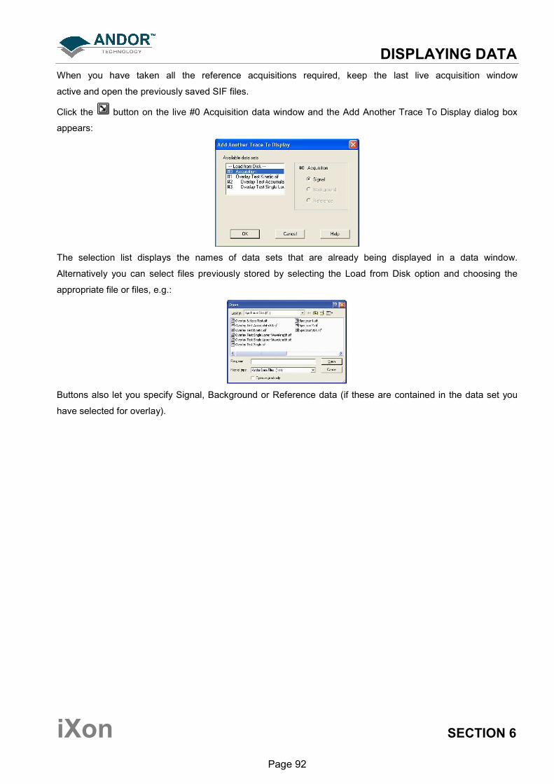
DISPLAYING DATA
iXon SECTION 6
Page 92
When you have taken all the reference acquisitions required, keep the last live acquisition window
active and open the previously saved SIF files.
Click the button on the live #0 Acquisition data window and the Add Another Trace To Display dialog box
appears:
The selection list displays the names of data sets that are already being displayed in a data window.
Alternatively you can select files previously stored by selecting the Load from Disk option and choosing the
appropriate file or files, e.g.:
Buttons also let you specify Signal, Background or Reference data (if these are contained in the data set you
have selected for overlay).
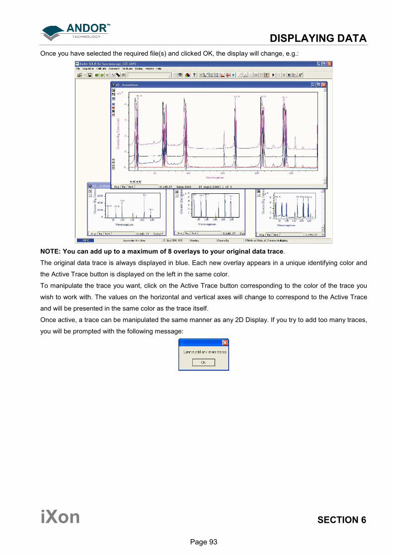
DISPLAYING DATA
iXon SECTION 6
Page 93
Once you have selected the required file(s) and clicked OK, the display will change, e.g.:
NOTE: You can add up to a maximum of 8 overlays to your original data trace.
The original data trace is always displayed in blue. Each new overlay appears in a unique identifying color and
the Active Trace button is displayed on the left in the same color.
To manipulate the trace you want, click on the Active Trace button corresponding to the color of the trace you
wish to work with. The values on the horizontal and vertical axes will change to correspond to the Active Trace
and will be presented in the same color as the trace itself.
Once active, a trace can be manipulated the same manner as any 2D Display. If you try to add too many traces,
you will be prompted with the following message:
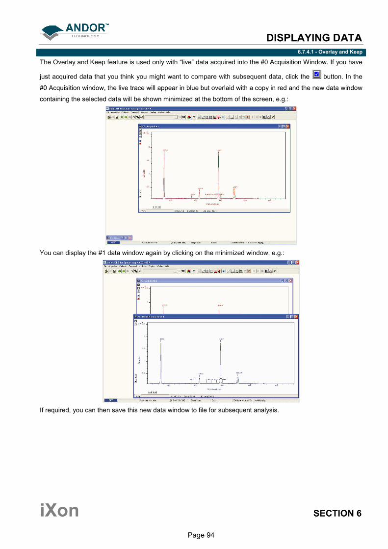
DISPLAYING DATA
iXon SECTION 6
Page 94
6.7.4.1 - Overlay and Keep
The Overlay and Keep feature is used only with “live” data acquired into the #0 Acquisition Window. If you have
just acquired data that you think you might want to compare with subsequent data, click the button. In the
#0 Acquisition window, the live trace will appear in blue but overlaid with a copy in red and the new data window
containing the selected data will be shown minimized at the bottom of the screen, e.g.:
You can display the #1 data window again by clicking on the minimized window, e.g.:
If required, you can then save this new data window to file for subsequent analysis.
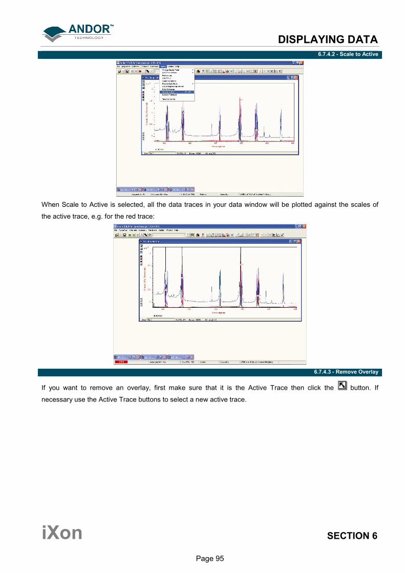
DISPLAYING DATA
iXon SECTION 6
Page 95
6.7.4.2 - Scale to Active
When Scale to Active is selected, all the data traces in your data window will be plotted against the scales of
the active trace, e.g. for the red trace:
6.7.4.3 - Remove Overlay
If you want to remove an overlay, first make sure that it is the Active Trace then click the button. If
necessary use the Active Trace buttons to select a new active trace.

DISPLAYING DATA
iXon SECTION 6
Page 96
6.7.5 - Baseline Correction
With Baseline Correction, a series of points on a signal are selected through which a smooth, continuous
reference is obtained. This reference is subsequently subtracted from the original signal and the resultant
spectrum saved to a new data set.
To select the function, click the button and the Baseline correcting dialog box appears, e.g.:
The user can now enter and define customized baselines. The values to be subtracted are entered against
individual pixel numbers in the dialog box. The user can select whether to fit the data using polynomial or cubic
spline. The user can also select where the Corrected and Baseline data are stored. When the necessary
parameters have been set and the Apply button is clicked, other data windows will be generated as defined by
the user, e.g.:
Window #0 will show the raw data as acquired during the last acquisition, by default window #2 will show the
profile of the customized baseline to be subtracted off the raw data and window #1 will show the baseline
corrected data i.e. #0 - #2). The window number labels of the customized baseline profile and corrected data
can be adjusted by changing the numbers detailed in the Baseline correcting dialog box.

DISPLAYING DATA
iXon SECTION 6
Page 97
6.8 - 3D DISPLAY MODE
If you have acquired data in Imaging mode or as a Kinetic series you can view the traces taken from all the
rows or tracks on one set of axes in a data window. Select the 3D option from the Change Display
Mode option on the Display menu or click the button and a data window will appear e.g.:
Along with the x-axis (calibrated by default to represent pixels across the CCD-chip) and the data-axis
(calibrated by default in counts), you now see a 3rd (or y-axis) calibrated in rows or tracks, depending on the
acquisition mode you have selected.
To read off a data value on a particular trace, use the scroll bar on the data window to move the trace into the
plane delineated by the x- and data-axes, and click on the trace to position the cursor on the point of interest
(you may need to use the left and right arrow keys on your keyboard to position the cursor precisely).
The numeric display on the status bar along the bottom edge of the data window will indicate the series
member on which the cursor is positioned (“Kinetics”), along with the corresponding x- and data-values.
If your data set contains a series of images (each of which may represent data acquired in Kinetics Mode) you
will notice that the data window has two scroll bars, placed end to end. The upper scroll bar allows you to move
between the members of the series, while the lower scroll bar allows you to view the traces that make up the
particular member of the series.
NOTE: The Zooming, Scrolling and Reset functions are the same as 2D mode.

DISPLAYING DATA
iXon SECTION 6
Page 98
6.8.1 - 3D display mode preferences
When 3D display mode is selected, the following options are available from the Display preferences dialog box:
You can display multiple tracks either Overlaid:
or Stacked:
or at 45 degrees:
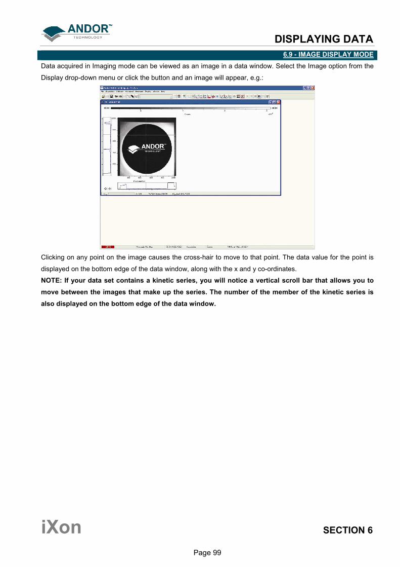
DISPLAYING DATA
iXon SECTION 6
Page 99
6.9 - IMAGE DISPLAY MODE
Data acquired in Imaging mode can be viewed as an image in a data window. Select the Image option from the
Display drop-down menu or click the button and an image will appear, e.g.:
Clicking on any point on the image causes the cross-hair to move to that point. The data value for the point is
displayed on the bottom edge of the data window, along with the x and y co-ordinates.
NOTE: If your data set contains a kinetic series, you will notice a vertical scroll bar that allows you to
move between the images that make up the series. The number of the member of the kinetic series is
also displayed on the bottom edge of the data window.
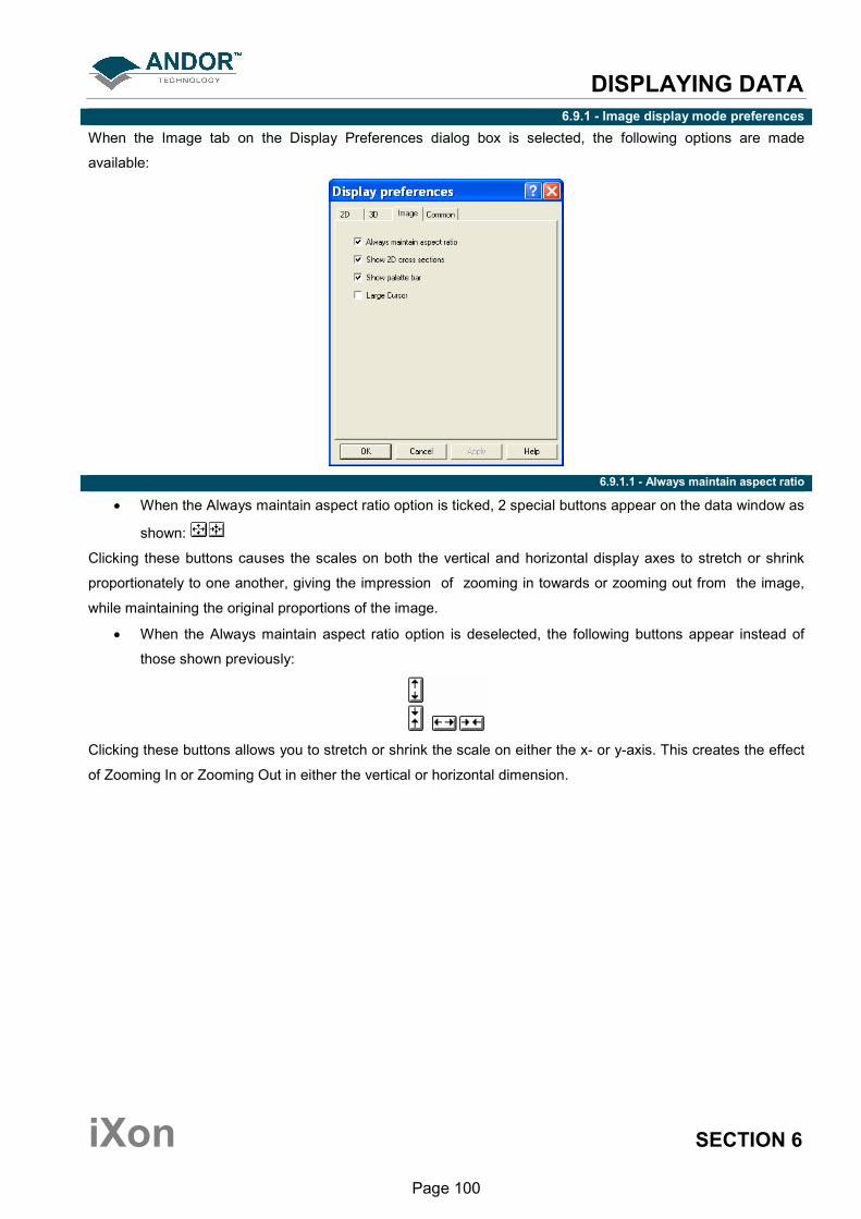
DISPLAYING DATA
iXon SECTION 6
Page 100
6.9.1 - Image display mode preferences
When the Image tab on the Display Preferences dialog box is selected, the following options are made
available:
6.9.1.1 - Always maintain aspect ratio
• When the Always maintain aspect ratio option is ticked, 2 special buttons appear on the data window as
shown:
Clicking these buttons causes the scales on both the vertical and horizontal display axes to stretch or shrink
proportionately to one another, giving the impression of zooming in towards or zooming out from the image,
while maintaining the original proportions of the image.
• When the Always maintain aspect ratio option is deselected, the following buttons appear instead of
those shown previously:
Clicking these buttons allows you to stretch or shrink the scale on either the x- or y-axis. This creates the effect
of Zooming In or Zooming Out in either the vertical or horizontal dimension.
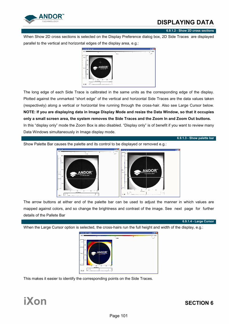
DISPLAYING DATA
iXon SECTION 6
Page 101
6.9.1.2 - Show 2D cross sections
When Show 2D cross sections is selected on the Display Preference dialog box, 2D Side Traces are displayed
parallel to the vertical and horizontal edges of the display area, e.g.:
The long edge of each Side Trace is calibrated in the same units as the corresponding edge of the display.
Plotted against the unmarked “short edge” of the vertical and horizontal Side Traces are the data values taken
(respectively) along a vertical or horizontal line running through the cross-hair. Also see Large Cursor below.
NOTE: If you are displaying data in Image Display Mode and resize the Data Window, so that it occupies
only a small screen area, the system removes the Side Traces and the Zoom In and Zoom Out buttons.
In this “display only” mode the Zoom Box is also disabled. “Display only” is of benefit if you want to review many
Data Windows simultaneously in Image display mode.
6.9.1.3 - Show palette bar
Show Palette Bar causes the palette and its control to be displayed or removed e.g.:
The arrow buttons at either end of the palette bar can be used to adjust the manner in which values are
mapped against colors, and so change the brightness and contrast of the image. See next page for further
details of the Pallete Bar
6.9.1.4 - Large Cursor
When the Large Cursor option is selected, the cross-hairs run the full height and width of the display, e.g.:
This makes it easier to identify the corresponding points on the Side Traces.
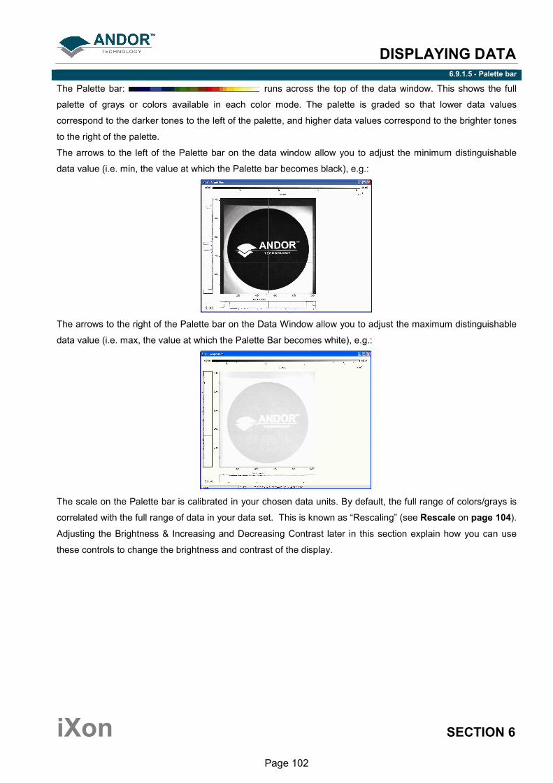
DISPLAYING DATA
iXon SECTION 6
Page 102
6.9.1.5 - Palette bar
The Palette bar: runs across the top of the data window. This shows the full
palette of grays or colors available in each color mode. The palette is graded so that lower data values
correspond to the darker tones to the left of the palette, and higher data values correspond to the brighter tones
to the right of the palette.
The arrows to the left of the Palette bar on the data window allow you to adjust the minimum distinguishable
data value (i.e. min, the value at which the Palette bar becomes black), e.g.:
The arrows to the right of the Palette bar on the Data Window allow you to adjust the maximum distinguishable
data value (i.e. max, the value at which the Palette Bar becomes white), e.g.:
The scale on the Palette bar is calibrated in your chosen data units. By default, the full range of colors/grays is
correlated with the full range of data in your data set. This is known as “Rescaling” (see Rescale on page 104).
Adjusting the Brightness & Increasing and Decreasing Contrast later in this section explain how you can use
these controls to change the brightness and contrast of the display.
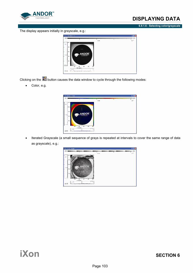
DISPLAYING DATA
iXon SECTION 6
Page 103
6.9.1.6 - Selecting color/grayscale
The display appears initially in grayscale, e.g.:
Clicking on the button causes the data window to cycle through the following modes:
• Color, e.g.
• Iterated Grayscale (a small sequence of grays is repeated at intervals to cover the same range of data
as grayscale), e.g.:
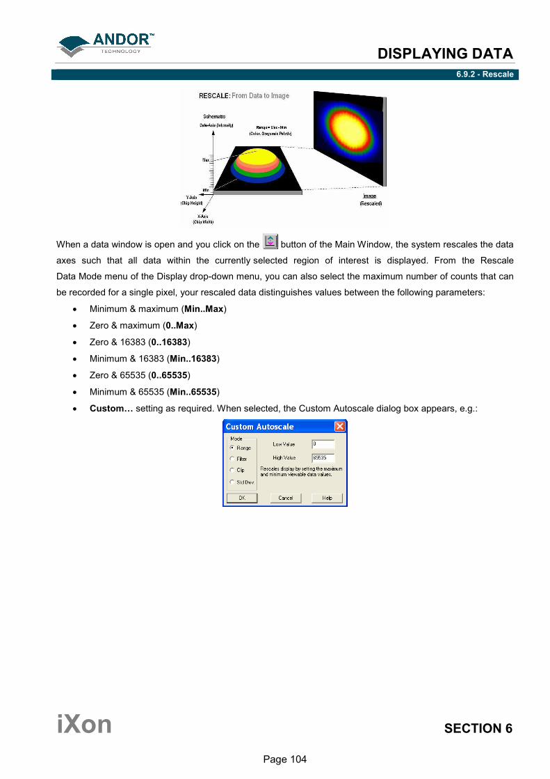
DISPLAYING DATA
iXon SECTION 6
Page 104
6.9.2 - Rescale
When a data window is open and you click on the button of the Main Window, the system rescales the data
axes such that all data within the currently selected region of interest is displayed. From the Rescale
Data Mode menu of the Display drop-down menu, you can also select the maximum number of counts that can
be recorded for a single pixel, your rescaled data distinguishes values between the following parameters:
• Minimum & maximum (Min..Max)
• Zero & maximum (0..Max)
• Zero & 16383 (0..16383)
• Minimum & 16383 (Min..16383)
• Zero & 65535 (0..65535)
• Minimum & 65535 (Min..65535)
• Custom… setting as required. When selected, the Custom Autoscale dialog box appears, e.g.:
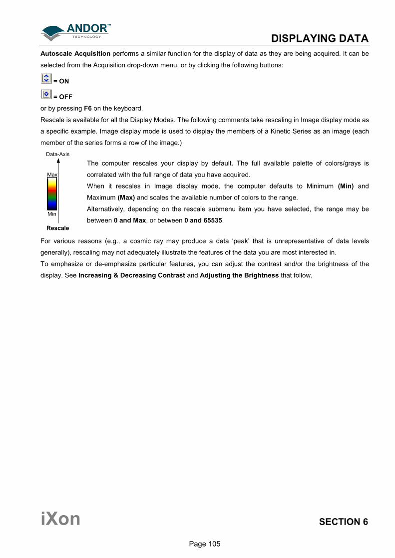
DISPLAYING DATA
iXon SECTION 6
Page 105
Autoscale Acquisition performs a similar function for the display of data as they are being acquired. It can be
selected from the Acquisition drop-down menu, or by clicking the following buttons:
= ON
= OFF
or by pressing F6 on the keyboard.
Rescale is available for all the Display Modes. The following comments take rescaling in Image display mode as
a specific example. Image display mode is used to display the members of a Kinetic Series as an image (each
member of the series forms a row of the image.)
Data-Axis
Rescale
Max
Min
The computer rescales your display by default. The full available palette of colors/grays is
correlated with the full range of data you have acquired.
When it rescales in Image display mode, the computer defaults to Minimum (Min) and
Maximum (Max) and scales the available number of colors to the range.
Alternatively, depending on the rescale submenu item you have selected, the range may be
between 0 and Max, or between 0 and 65535.
For various reasons (e.g., a cosmic ray may produce a data ‘peak’ that is unrepresentative of data levels
generally), rescaling may not adequately illustrate the features of the data you are most interested in.
To emphasize or de-emphasize particular features, you can adjust the contrast and/or the brightness of the
display. See Increasing & Decreasing Contrast and Adjusting the Brightness that follow.

DISPLAYING DATA
iXon SECTION 6
Page 106
6.9.3 - High & Low contrast overview
Data-Axis
High Contrast
Max
Min
Original
Data
Range
Assume your original data are rescaled. To achieve high contrast, the computer scales a
smaller range of data with the same number of colors as it used for rescaling.
Any data value greater than the maximum in the displayed data range is represented by the
brightest color (white). Any data value lower than the minimum in the displayed data range is
represented by the darkest color (black).
Now only a fraction of the original data range is represented by the total number of colors.
Decreasing the displayed data range produces high contrast.
Data-Axis
Low Contrast
Max
Min
Original
Data
Range
To achieve low contrast, the computer scales a larger range of data with the same number of
colors as it used for rescaling. Thus the original data are represented by a smaller range of
colors.
Increasing the displayed data range produces low contrast.

DISPLAYING DATA
iXon SECTION 6
Page 107
6.9.3.1 - Increasing & decreasing contrast
You can use the pairs of left-right arrows at either end of the Palette Bar to increase or decrease the displayed
data range (i.e. ‘shrink’ or ‘stretch’ the scale on the palette) and thereby alter the contrast of the data shown in
Image display mode. You can also use the + and – keys to do the same function.
Increasing the displayed data range (‘shrinking’ the scale).
Increase Displayed
Data Range
Decrease Contrast
Decreasing the displayed data range (‘stretching’ the scale).
Increase Contrast
Decrease Displayed
Data Range
By holding down the left-right arrows at either end of the Palette Bar you can alter the minimum and maximum
values in the displayed data range independently of each other, and so adjust the contrast to the level you require.
As you hold down the arrows (place the cursor over an arrow button and hold down the primary mouse button),
observe carefully how the scale changes and how the displayed data range is affected. If you wish to undo your
changes, use Rescale.
NOTE: When the left-right arrows are held down for a time, you will see the display flash periodically as
the system performs the contrast adjustment. These flashes occur as the system refreshes the color
palette to cover your new displayed data range. Hold the arrows down until you reach your required
contrast level.

DISPLAYING DATA
iXon SECTION 6
Page 108
6.9.4 - Brightness overview
Data-Axis
Brighter
Max
Min
Original
Data
Range
To make the data shown in Image display mode brighter, the computer uses the same
number of colors as it used for rescaling to scale lower data values.
Thus any data originally represented by darker colors are now represented by brighter
colors.
Data-Axis
Darker
Max
Min
Original
Data
Range
To make the data shown in Image Display Mode darker, the computer uses the same
number of colors as it used for rescaling to scale higher data values.
Thus any data originally represented by brighter colors are now represented by darker
colors.
NOTE: If you wish to undo your changes, use Rescale.
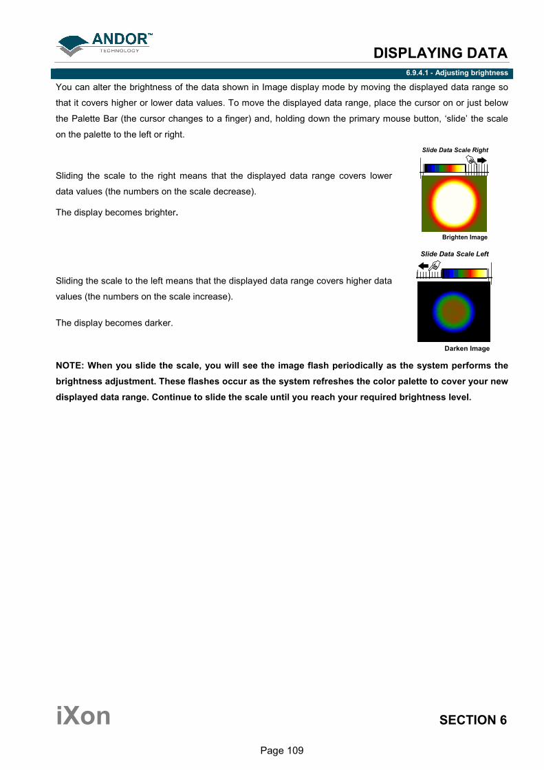
DISPLAYING DATA
iXon SECTION 6
Page 109
6.9.4.1 - Adjusting brightness
You can alter the brightness of the data shown in Image display mode by moving the displayed data range so
that it covers higher or lower data values. To move the displayed data range, place the cursor on or just below
the Palette Bar (the cursor changes to a finger) and, holding down the primary mouse button, ‘slide’ the scale
on the palette to the left or right.
Sliding the scale to the right means that the displayed data range covers lower
data values (the numbers on the scale decrease).
The display becomes brighter.
Slide Data Scale Right
Brighten Image
Sliding the scale to the left means that the displayed data range covers higher data
values (the numbers on the scale increase).
The display becomes darker.
Slide Data Scale Left
Darken Image
NOTE: When you slide the scale, you will see the image flash periodically as the system performs the
brightness adjustment. These flashes occur as the system refreshes the color palette to cover your new
displayed data range. Continue to slide the scale until you reach your required brightness level.

DISPLAYING DATA
iXon SECTION 6
Page 110
6.10 - DATA HISTOGRAM
The Data Histogram dialog Box is launched either by clicking on the icon on the Main Window, or
selecting Data Histogram from the Display drop-down menu. This tool allows you to plot a histogram, or graph,
between the maximum and minimum data points in the displayed range. It also contains a filter drop down
menu, which allows for more accurate analysis and presentation of data values.
By clicking on an open data window, its histogram will be displayed on the Data Histogram dialog. When
plotting the histogram, the focus is transferred to the new data window and the displayed histogram is that of
the plotted histogram. The data from which the histogram is displayed is indicated on the title bar of the Data
Histogram dialog. To return the focus on the original data, click on the original data window. Modes to view
specific areas of spectra can be selected through the drop-down menu:
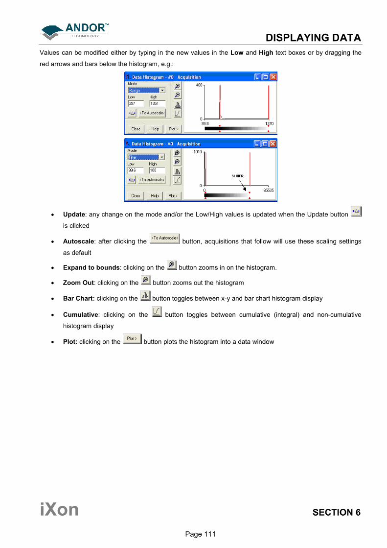
DISPLAYING DATA
iXon SECTION 6
Page 111
Values can be modified either by typing in the new values in the Low and High text boxes or by dragging the
red arrows and bars below the histogram, e.g.:
• Update: any change on the mode and/or the Low/High values is updated when the Update button
is clicked
• Autoscale: after clicking the button, acquisitions that follow will use these scaling settings
as default
• Expand to bounds: clicking on the button zooms in on the histogram.
• Zoom Out: clicking on the button zooms out the histogram
• Bar Chart: clicking on the button toggles between x-y and bar chart histogram display
• Cumulative: clicking on the button toggles between cumulative (integral) and non-cumulative
histogram display
• Plot: clicking on the button plots the histogram into a data window
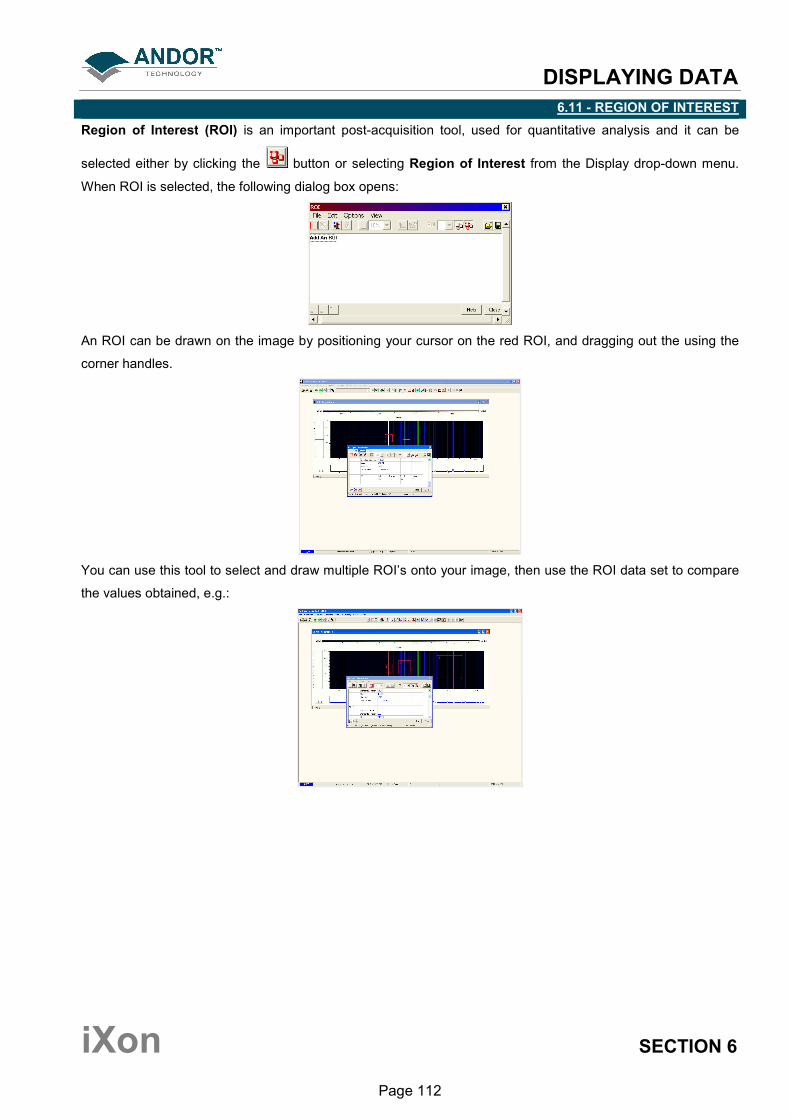
DISPLAYING DATA
iXon SECTION 6
Page 112
6.11 - REGION OF INTEREST
Region of Interest (ROI) is an important post-acquisition tool, used for quantitative analysis and it can be
selected either by clicking the button or selecting Region of Interest from the Display drop-down menu.
When ROI is selected, the following dialog box opens:
An ROI can be drawn on the image by positioning your cursor on the red ROI, and dragging out the using the
corner handles.
You can use this tool to select and draw multiple ROI’s onto your image, then use the ROI data set to compare
the values obtained, e.g.:
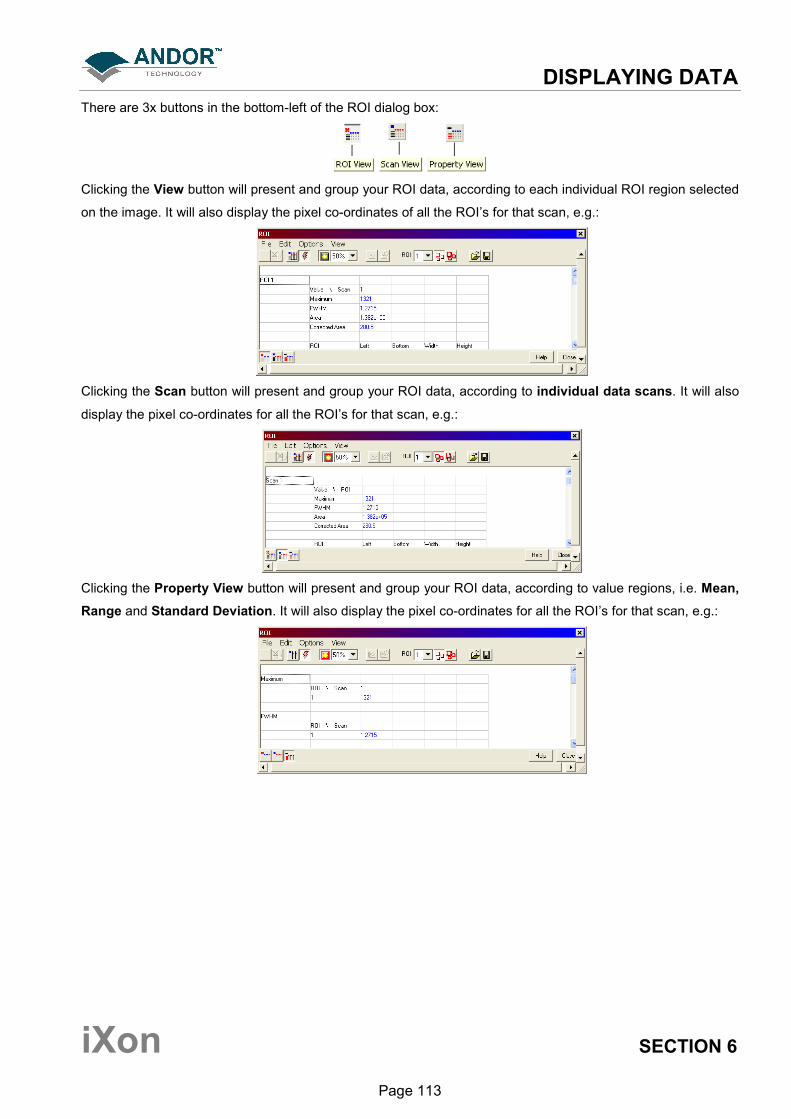
DISPLAYING DATA
iXon SECTION 6
Page 113
There are 3x buttons in the bottom-left of the ROI dialog box:
Clicking the View button will present and group your ROI data, according to each individual ROI region selected
on the image. It will also display the pixel co-ordinates of all the ROI’s for that scan, e.g.:
Clicking the Scan button will present and group your ROI data, according to individual data scans. It will also
display the pixel co-ordinates for all the ROI’s for that scan, e.g.:
Clicking the Property View button will present and group your ROI data, according to value regions, i.e. Mean,
Range and Standard Deviation. It will also display the pixel co-ordinates for all the ROI’s for that scan, e.g.:
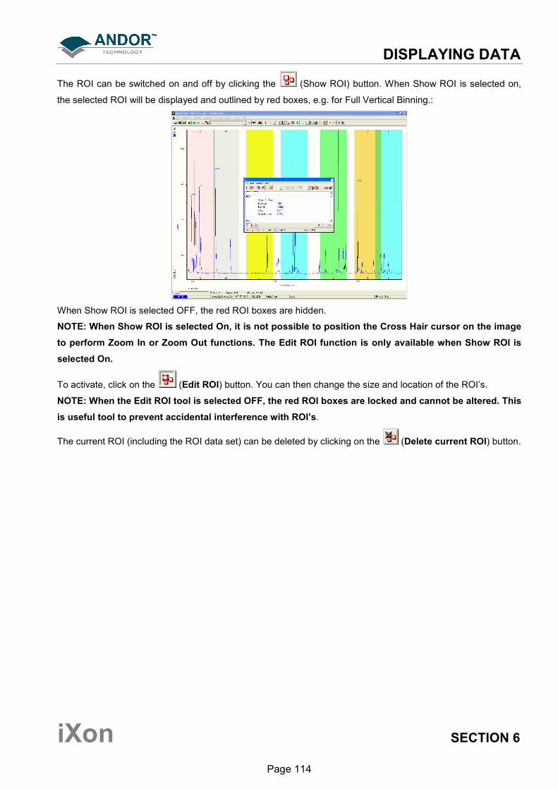
DISPLAYING DATA
iXon SECTION 6
Page 114
The ROI can be switched on and off by clicking the (Show ROI) button. When Show ROI is selected on,
the selected ROI will be displayed and outlined by red boxes, e.g. for Full Vertical Binning.:
When Show ROI is selected OFF, the red ROI boxes are hidden.
NOTE: When Show ROI is selected On, it is not possible to position the Cross Hair cursor on the image
to perform Zoom In or Zoom Out functions. The Edit ROI function is only available when Show ROI is
selected On.
To activate, click on the (Edit ROI) button. You can then change the size and location of the ROI’s.
NOTE: When the Edit ROI tool is selected OFF, the red ROI boxes are locked and cannot be altered. This
is useful tool to prevent accidental interference with ROI’s.
The current ROI (including the ROI data set) can be deleted by clicking on the (Delete current ROI) button.
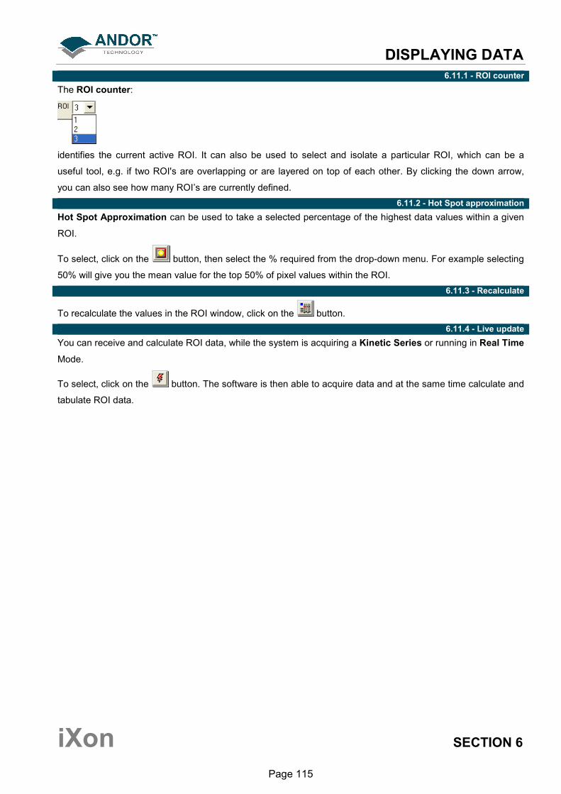
DISPLAYING DATA
iXon SECTION 6
Page 115
6.11.1 - ROI counter
The ROI counter:
identifies the current active ROI. It can also be used to select and isolate a particular ROI, which can be a
useful tool, e.g. if two ROI's are overlapping or are layered on top of each other. By clicking the down arrow,
you can also see how many ROI’s are currently defined.
6.11.2 - Hot Spot approximation
Hot Spot Approximation can be used to take a selected percentage of the highest data values within a given
ROI.
To select, click on the button, then select the % required from the drop-down menu. For example selecting
50% will give you the mean value for the top 50% of pixel values within the ROI.
6.11.3 - Recalculate
To recalculate the values in the ROI window, click on the button.
6.11.4 - Live update
You can receive and calculate ROI data, while the system is acquiring a Kinetic Series or running in Real Time
Mode.
To select, click on the button. The software is then able to acquire data and at the same time calculate and
tabulate ROI data.
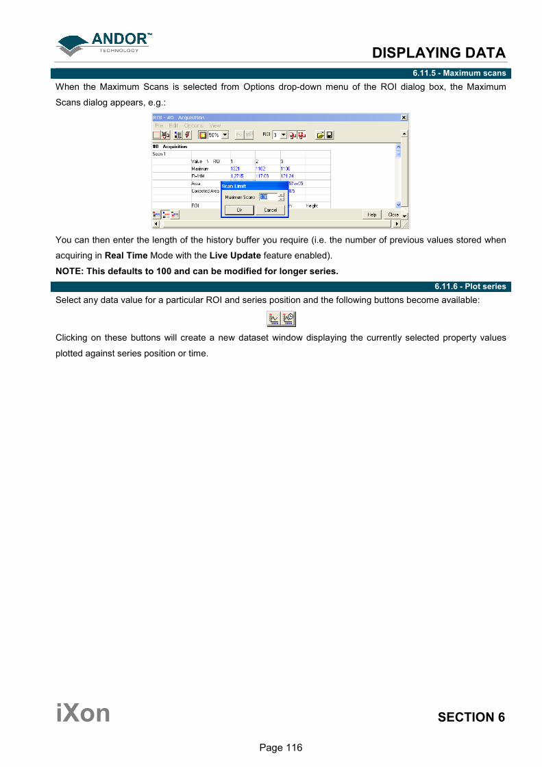
DISPLAYING DATA
iXon SECTION 6
Page 116
6.11.5 - Maximum scans
When the Maximum Scans is selected from Options drop-down menu of the ROI dialog box, the Maximum
Scans dialog appears, e.g.:
You can then enter the length of the history buffer you require (i.e. the number of previous values stored when
acquiring in Real Time Mode with the Live Update feature enabled).
NOTE: This defaults to 100 and can be modified for longer series.
6.11.6 - Plot series
Select any data value for a particular ROI and series position and the following buttons become available:
Clicking on these buttons will create a new dataset window displaying the currently selected property values
plotted against series position or time.

DISPLAYING DATA
iXon SECTION 6
Page 117
6.12 - TIME STAMP
When the button is clicked, the Display Preferences dialog box opens, e.g.:
The Time Stamp feature allows you to add to the display the time at which the acquisition, or each scan in a
kinetic series, occurred., e.g.:
Time & date information, or time relative to the start of the acquisition can be displayed by selecting Enabled,
then selecting the appropriate option in the Style drop down list.
• The position of the time stamp within the display can be set by adjusting the Vertical & Horizontal
Alignment controls.
• The Color of the text can also be changed
• The time can be made to print on a solid background by de-selecting Transparent.
To remove the Time Stamp from the display de-select Enabled.

DISPLAYING DATA
iXon SECTION 6
Page 118
6.13 - PLAYBACK
After a Kinetic series acquisition has been has been taken, it can be played back again for analysis.
• To replay, click the button and the acquisition will display again as taken
• To pause, click the button
• To stop click the button Playback autoscale performs a similar function to Autoscale acquisition and is selected from the button on the
top of the main window ( = ON, = OFF).
The sequence can also be viewed with different parameters set.
Select Sequence options from the Display drop-down menu and the Sequence Setup dialog box appears,
e.g.:
Select the parameters as required, click OK then playback the sequence as normal.
NOTE: This can be exported as an MPEG or other similar file for use in presentations, etc. Please refer
to Section 7 for further details of handling files.
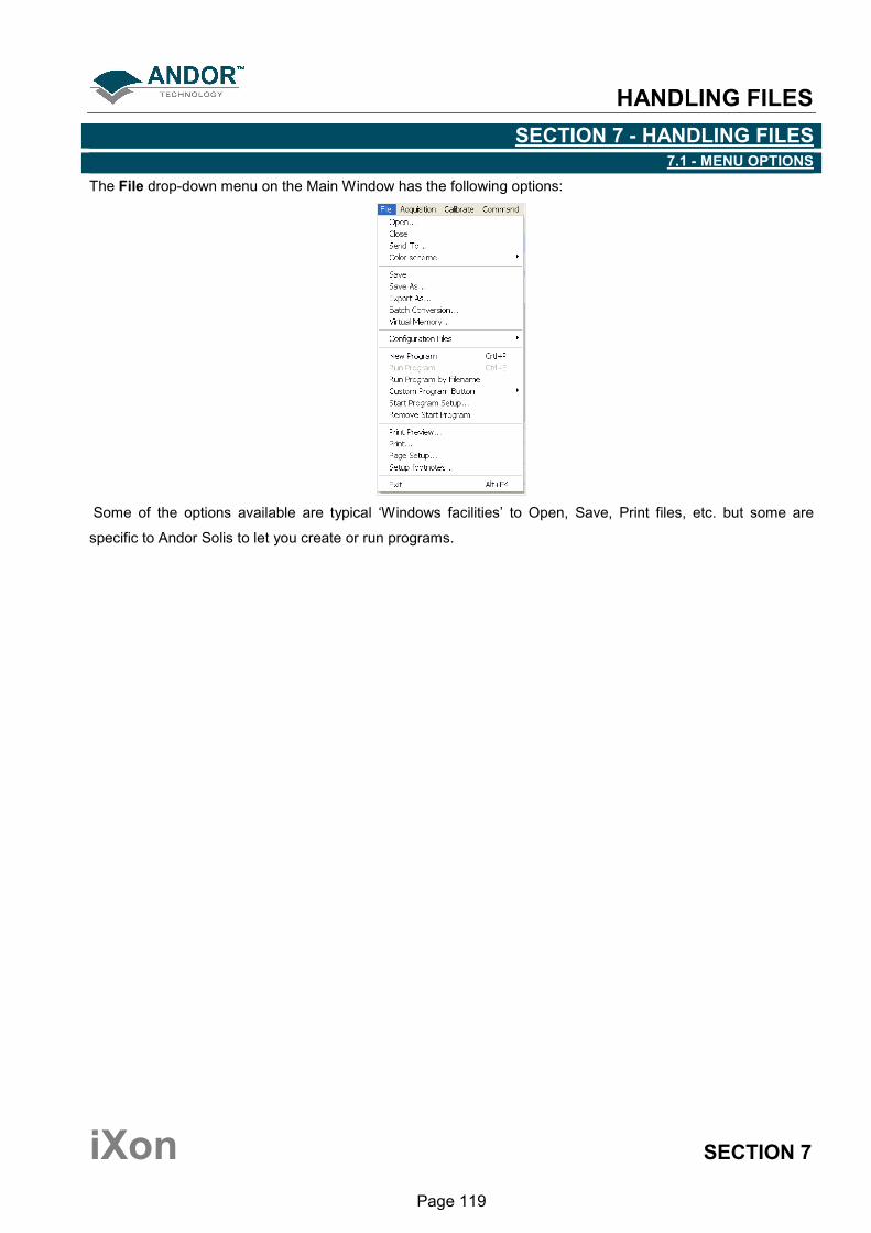
HANDLING FILES
iXon SECTION 7
Page 119
SECTION 7 - HANDLING FILES 7.1 - MENU OPTIONS
The File drop-down menu on the Main Window has the following options:
Some of the options available are typical ‘Windows facilities’ to Open, Save, Print files, etc. but some are
specific to Andor Solis to let you create or run programs.
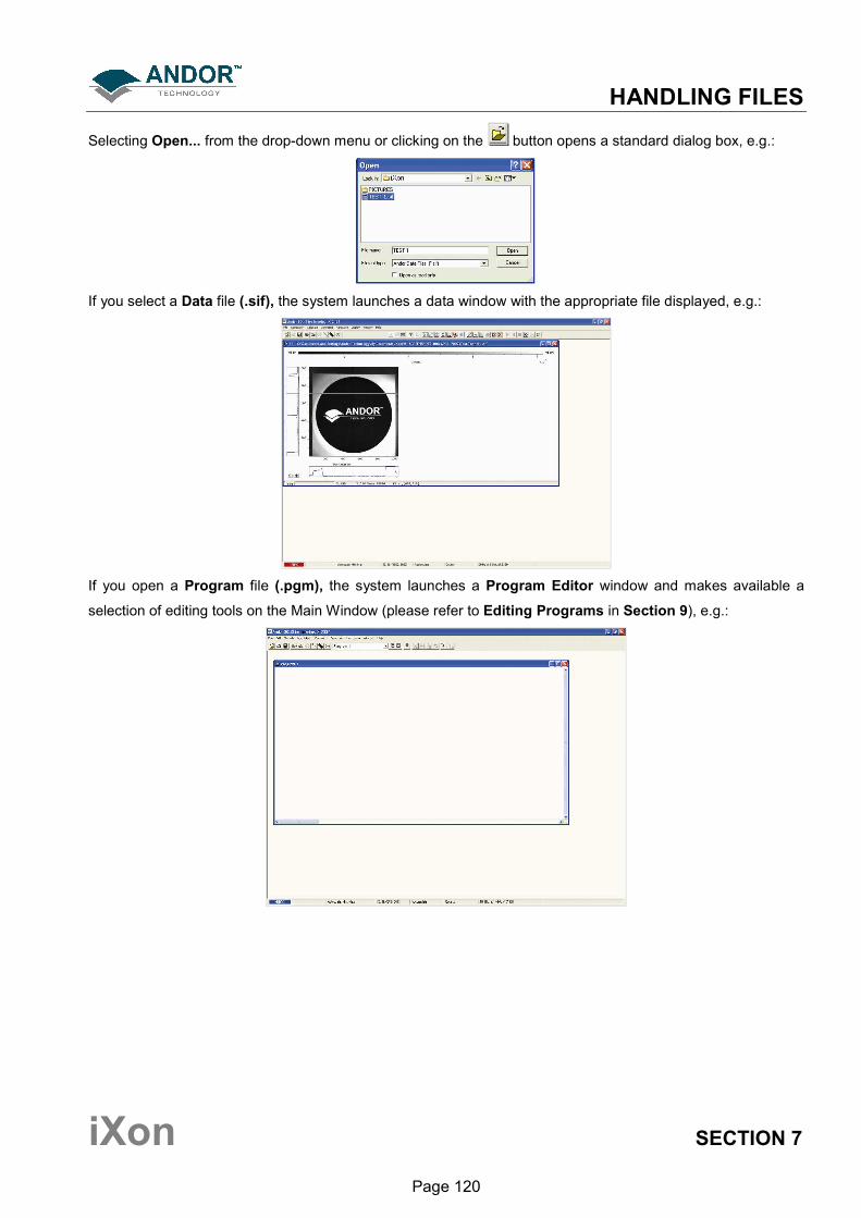
HANDLING FILES
iXon SECTION 7
Page 120
Selecting Open... from the drop-down menu or clicking on the button opens a standard dialog box, e.g.:
If you select a Data file (.sif), the system launches a data window with the appropriate file displayed, e.g.:
If you open a Program file (.pgm), the system launches a Program Editor window and makes available a
selection of editing tools on the Main Window (please refer to Editing Programs in Section 9), e.g.:

HANDLING FILES
iXon SECTION 7
Page 121
7.1.1 - Close
Close removes the active Data Window or Program Editor Window from the Main Window. You will be
prompted to save any unsaved data to an appropriate filename.
7.1.2 - Save
Selecting Save or stores the contents of an active and previously saved Data Window or Program Editor
Window under the current filename.
7.1.3 - Save As
Save as... launches the Save As dialog box, which lets you save the contents of an active Data Window or
Program Editor Window under a filename and in a directory of your choice.
NOTE: If data is saved as a .sif file, the information contained within file information is saved. If the data
is exported to another file type, the information within file information is lost

HANDLING FILES
iXon SECTION 7
Page 122
7.2 - EXPORT AS
Export As… opens the Export As dialog box, e.g.:
Depending on the Display & Readout modes selected, the file can be saved in one or more of the following
formats:
• ASCII (.asc)
• Bitmap (.bmp)
• GRAMS (.spc)
• Raw data (.dat)
• TIFF (.tif)
Table 10 shows a matrix of the actual combinations available:
Table 10: File export combinations
Readout mode Display mode ASCII Bitmap GRAMS Raw data TIFF
Image Image
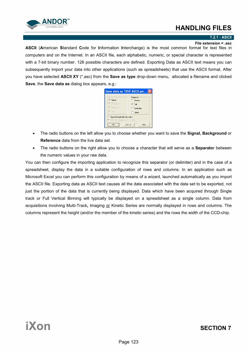
HANDLING FILES
iXon SECTION 7
Page 123
7.2.1 - ASCII
File extension = .asc
ASCII (American Standard Code for Information Interchange) is the most common format for text files in
computers and on the Internet. In an ASCII file, each alphabetic, numeric, or special character is represented
with a 7-bit binary number. 128 possible characters are defined. Exporting Data as ASCII text means you can
subsequently import your data into other applications (such as spreadsheets) that use the ASCII format. After
you have selected ASCII XY (*.asc) from the Save as type drop-down menu, allocated a filename and clicked
Save, the Save data as dialog box appears, e.g.:
• The radio buttons on the left allow you to choose whether you want to save the Signal, Background or
Reference data from the live data set.
• The radio buttons on the right allow you to choose a character that will serve as a Separator between
the numeric values in your raw data.
You can then configure the importing application to recognize this separator (or delimiter) and in the case of a
spreadsheet, display the data in a suitable configuration of rows and columns. In an application such as
Microsoft Excel you can perform this configuration by means of a wizard, launched automatically as you import
the ASCII file. Exporting data as ASCII text causes all the data associated with the data set to be exported, not
just the portion of the data that is currently being displayed. Data which have been acquired through Single
track or Full Vertical Binning will typically be displayed on a spreadsheet as a single column. Data from
acquisitions involving Multi-Track, Imaging or Kinetic Series are normally displayed in rows and columns. The
columns represent the height (and/or the member of the kinetic series) and the rows the width of the CCD-chip.
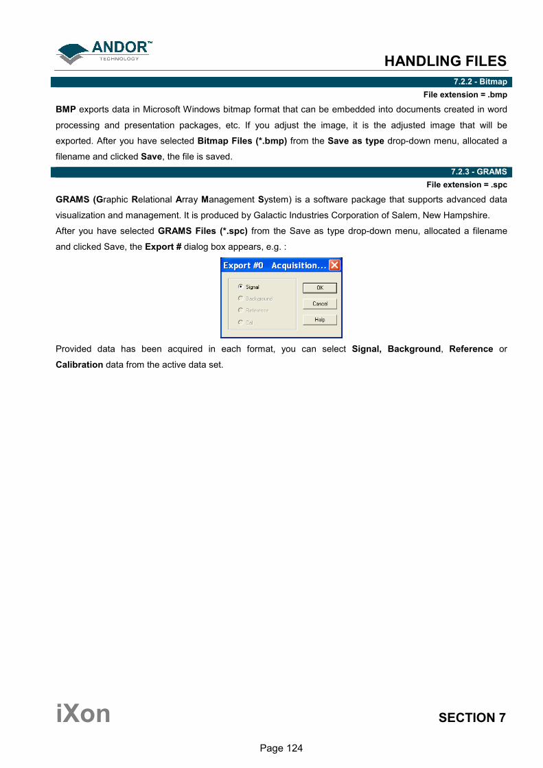
HANDLING FILES
iXon SECTION 7
Page 124
7.2.2 - Bitmap
File extension = .bmp
BMP exports data in Microsoft Windows bitmap format that can be embedded into documents created in word
processing and presentation packages, etc. If you adjust the image, it is the adjusted image that will be
exported. After you have selected Bitmap Files (*.bmp) from the Save as type drop-down menu, allocated a
filename and clicked Save, the file is saved.
7.2.3 - GRAMS
File extension = .spc
GRAMS (Graphic Relational Array Management System) is a software package that supports advanced data
visualization and management. It is produced by Galactic Industries Corporation of Salem, New Hampshire.
After you have selected GRAMS Files (*.spc) from the Save as type drop-down menu, allocated a filename
and clicked Save, the Export # dialog box appears, e.g. :
Provided data has been acquired in each format, you can select Signal, Background, Reference or
Calibration data from the active data set.
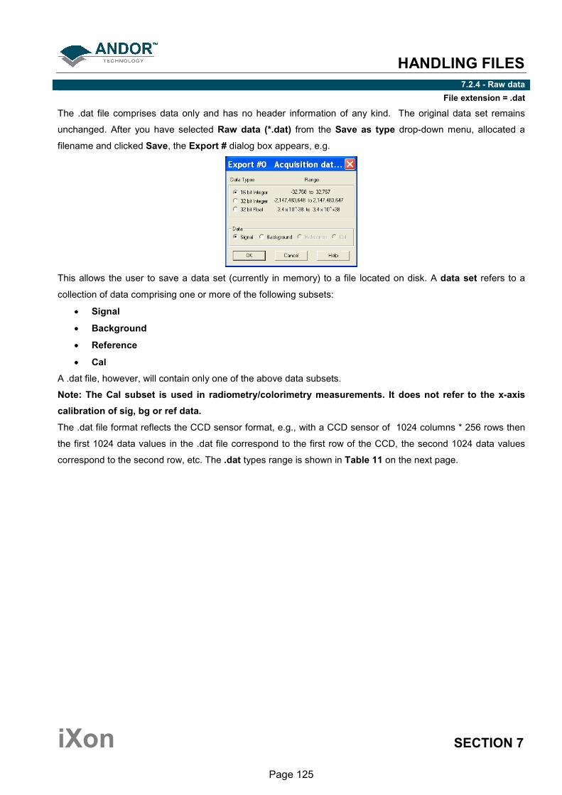
HANDLING FILES
iXon SECTION 7
Page 125
7.2.4 - Raw data
File extension = .dat
The .dat file comprises data only and has no header information of any kind. The original data set remains
unchanged. After you have selected Raw data (*.dat) from the Save as type drop-down menu, allocated a
filename and clicked Save, the Export # dialog box appears, e.g.
This allows the user to save a data set (currently in memory) to a file located on disk. A data set refers to a
collection of data comprising one or more of the following subsets:
• Signal
• Background
• Reference
• Cal
A .dat file, however, will contain only one of the above data subsets.
Note: The Cal subset is used in radiometry/colorimetry measurements. It does not refer to the x-axis
calibration of sig, bg or ref data.
The .dat file format reflects the CCD sensor format, e.g., with a CCD sensor of 1024 columns * 256 rows then
the first 1024 data values in the .dat file correspond to the first row of the CCD, the second 1024 data values
correspond to the second row, etc. The .dat types range is shown in Table 11 on the next page.

HANDLING FILES
iXon SECTION 7
Page 126
Table 11: .dat types
Data type
No. of
bytes Range
(1) 16 bit
integer 2
-32,768 to 32,767
(2) 32 bit
integer 4 -2,147,483,648 to 2,147,483,647
(3) 32 bit float 4 3.4 x 10-38
to 3.4 x 10+38
(1) Saves a data set to a 16 bit integer .dat file. Note: if a data value exceeds the limits of a 16 bit integer (<-
32,768 or > 32,767), that data value is truncated to the corresponding limit (e.g. if a data value is 36,000
units then the value is truncated to 32,767 units).
(2) Saves a data set to a 32 bit integer .dat file. The limits for the 32 bit integer are handled in similar fashion to
the 16 bit integer above.
(3) Saves a data set to a 32 bit floating point .dat file. When using your own software to handle a .dat file, you have to work out how many bytes to read in. Each 32
bit value requires 4 bytes to handle the value. Thus, for example, to read in a 32 bit .dat file consisting of 1024
data values, you would have to read in 4096 bytes in total.
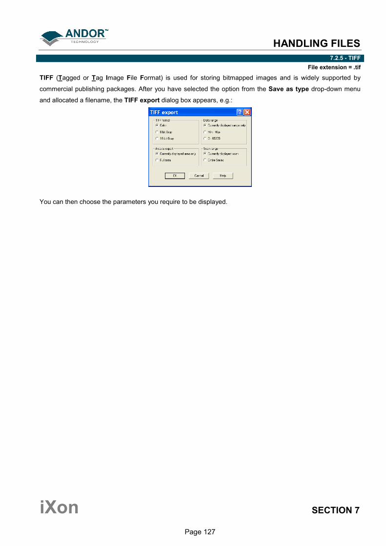
HANDLING FILES
iXon SECTION 7
Page 127
7.2.5 - TIFF
File extension = .tif
TIFF (Tagged or Tag Image File Format) is used for storing bitmapped images and is widely supported by
commercial publishing packages. After you have selected the option from the Save as type drop-down menu
and allocated a filename, the TIFF export dialog box appears, e.g.:
You can then choose the parameters you require to be displayed.
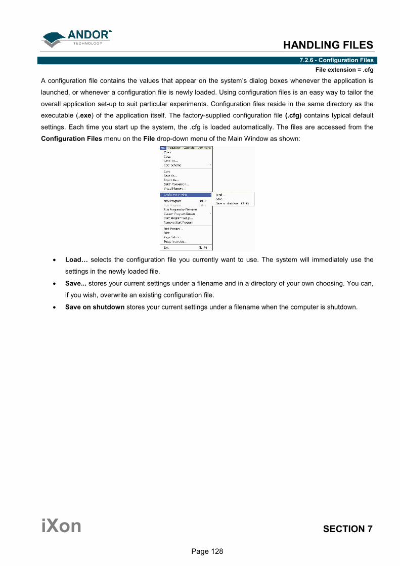
HANDLING FILES
iXon SECTION 7
Page 128
7.2.6 - Configuration Files
File extension = .cfg
A configuration file contains the values that appear on the system’s dialog boxes whenever the application is
launched, or whenever a configuration file is newly loaded. Using configuration files is an easy way to tailor the
overall application set-up to suit particular experiments. Configuration files reside in the same directory as the
executable (.exe) of the application itself. The factory-supplied configuration file (.cfg) contains typical default
settings. Each time you start up the system, the .cfg is loaded automatically. The files are accessed from the
Configuration Files menu on the File drop-down menu of the Main Window as shown:
• Load… selects the configuration file you currently want to use. The system will immediately use the
settings in the newly loaded file.
• Save... stores your current settings under a filename and in a directory of your own choosing. You can,
if you wish, overwrite an existing configuration file.
• Save on shutdown stores your current settings under a filename when the computer is shutdown.
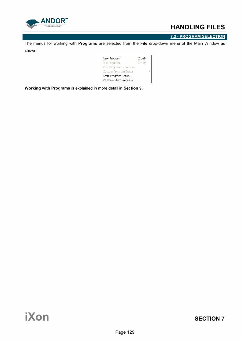
HANDLING FILES
iXon SECTION 7
Page 129
7.3 - PROGRAM SELECTION
The menus for working with Programs are selected from the File drop-down menu of the Main Window as
shown:
Working with Programs is explained in more detail in Section 9.

CALIBRATION
iXon SECTION 8
Page 130
SECTION 8 - CALIBRATION 8.1 - CALIBRATION OPTIONS
The following calibration options for data displays are available from the Calibration Menu on the Main
Window:
• Manual X-Calibration: allows calibration of the x-axis of data displays by manually setting values
(time, pixel number, wavelength, Raman shift or spatial position) against recognizable features of a
particular 2D data trace.
• X-Calibration by Spectrograph: allows calibration of the x-axis of your data displays with reference to
your spectrograph’s specifications. Calibration may be in wavelength or Raman shift.
• Change Units: lets you change the units on the x-axis of a data display (e.g. nm to µm, cm to pixel
number, etc.)
In addition, the option Remove X-Calibration has 2 further options as follows:
1. Current Data returns the data in the active Data Window to its default pixel x-calibration
2. New Acquisitions causes future data to be acquired with the default pixel x-calibration
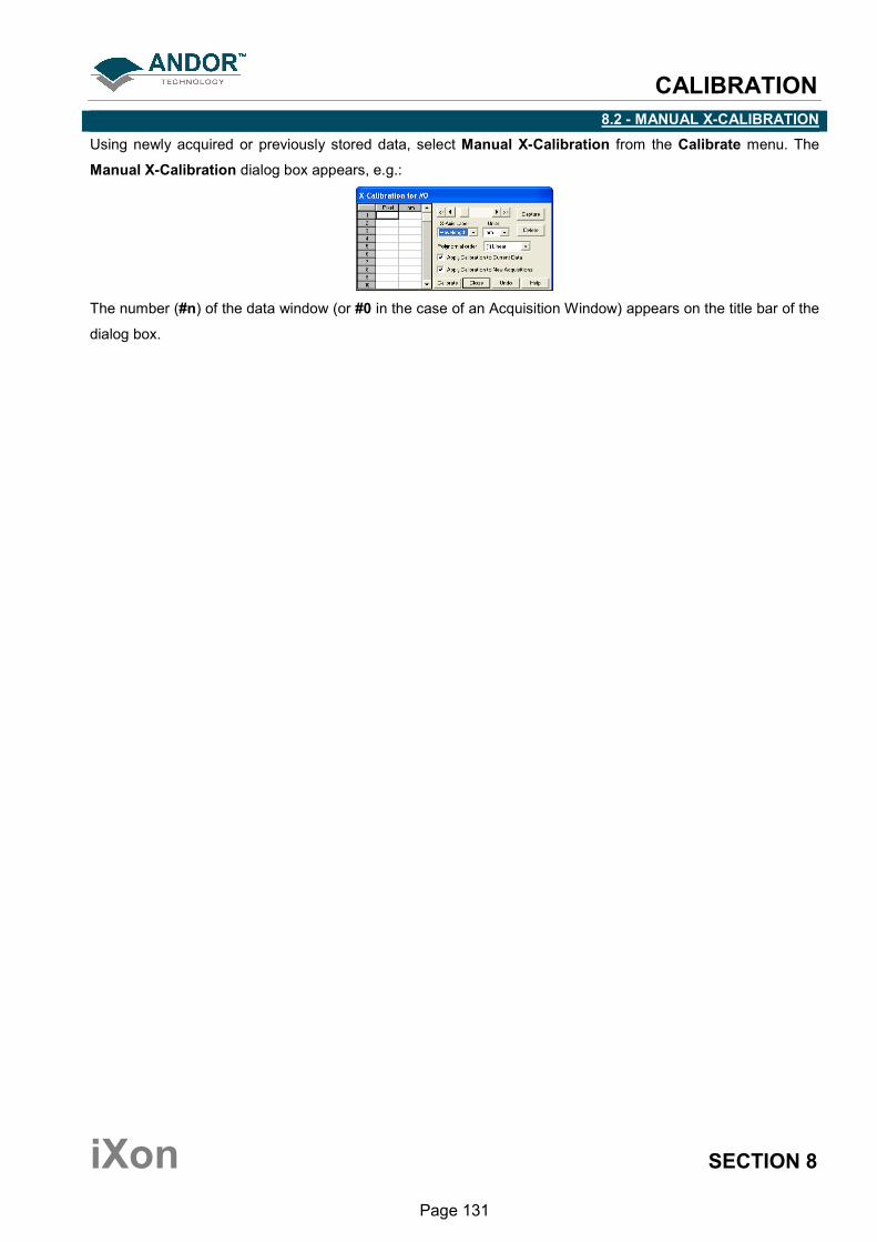
CALIBRATION
iXon SECTION 8
Page 131
8.2 - MANUAL X-CALIBRATION
Using newly acquired or previously stored data, select Manual X-Calibration from the Calibrate menu. The
Manual X-Calibration dialog box appears, e.g.:
The number (#n) of the data window (or #0 in the case of an Acquisition Window) appears on the title bar of the
dialog box.

CALIBRATION
iXon SECTION 8
Page 132
8.2.1 - Supplying calibration details
To manually calibrate a data window, first use the drop-down lists on the Manual X-Calibration dialog box to
choose the label and the units you wish to use for the x-axis. The available labels and units are shown in
Table 12 below. Your chosen unit will appear on the top of the right-hand column of the two columns to the left
of the Manual X-Calibration dialog box.
Table 12: Labels & Units
X-AXIS LABEL UNITS
Wavelength nm, µm, cm-1
, eV
Raman Shift cm-1
Position µm, mm, cm, µi(nches), in(ches)
Time ms, secs
Pixel pixels
Another drop-down list allows you to choose a polynomial order for your calibration. The following polynomial
options are available:
POLYNOMIAL ORDER
DESCRIPTION
Linear The linear fit is best for situations where only 2 or 3 spectral features can be
identified.
Quadratic A quadratic polynomial produces the best calibration fit if the known spectral
features are located near the center of the CCD sensor.
Cubic A cubic polynomial produces the best calibration fit if the known spectral
features are evenly distributed across the CCD sensor.
To perform the calibration:
1. Place the cross-hairs on a feature which you know to have a particular x-axis value and click Capture.
If you wish to remove a point that you had previously selected, click Delete.
2. The pixel number will appear in the left-hand column. Against it, in the right-hand column, enter a value.
3. Repeat steps 1 and 2 for at least one other point. However, to achieve a good quality calibration you
should choose a polynomial order fit commensurate with the spread of known spectral features across
your sensor.
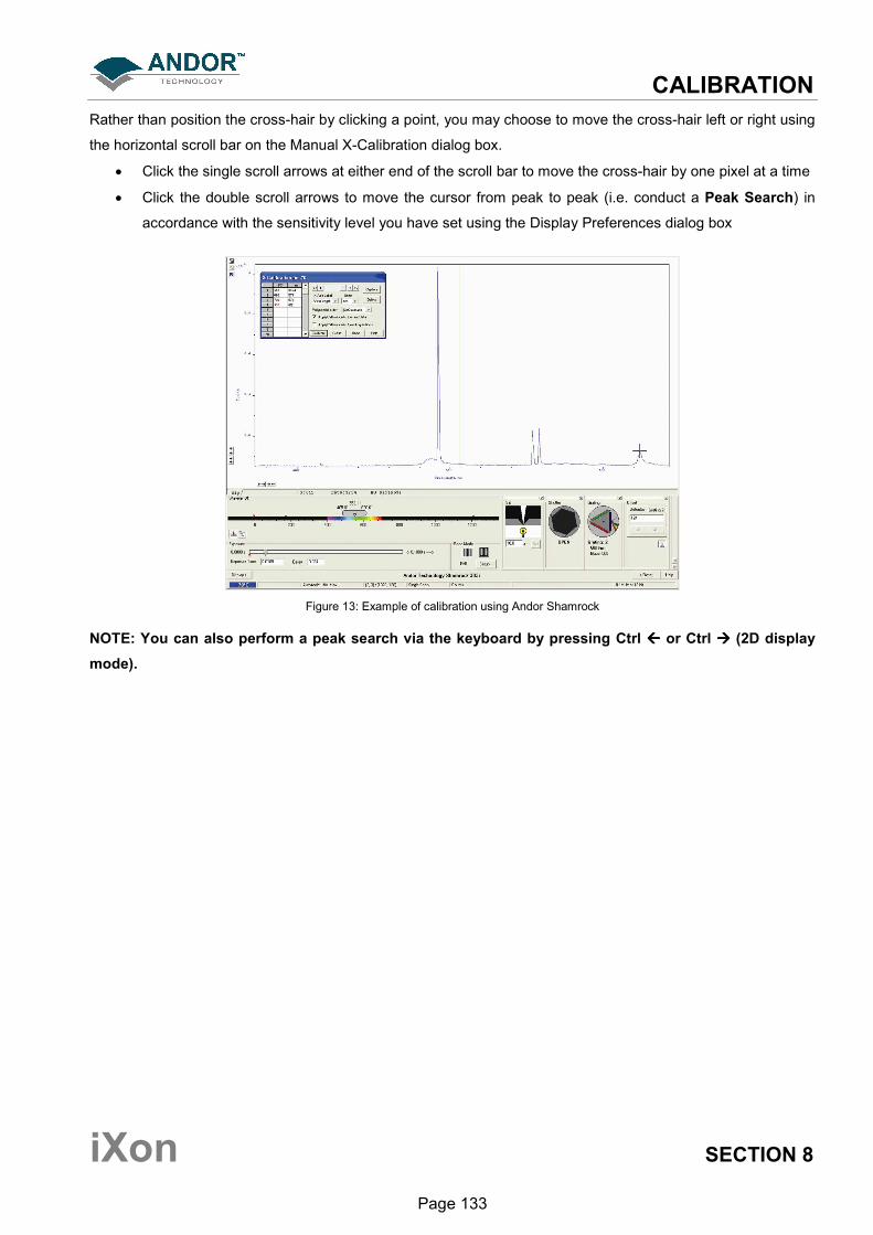
CALIBRATION
iXon SECTION 8
Page 133
Rather than position the cross-hair by clicking a point, you may choose to move the cross-hair left or right using
the horizontal scroll bar on the Manual X-Calibration dialog box.
• Click the single scroll arrows at either end of the scroll bar to move the cross-hair by one pixel at a time
• Click the double scroll arrows to move the cursor from peak to peak (i.e. conduct a Peak Search) in
accordance with the sensitivity level you have set using the Display Preferences dialog box
Figure 13: Example of calibration using Andor Shamrock
NOTE: You can also perform a peak search via the keyboard by pressing Ctrl or Ctrl (2D display
mode).

CALIBRATION
iXon SECTION 8
Page 134
8.2.2 - Applying calibration 8.2.2.1 - Calibrate
Depending on the selections made using the check boxes on the Manual X-Calibration dialog box, clicking the
Calibrate button will apply calibration to the active data window and/or to future data acquisitions.
In the event that Manual X-Calibration fails, it typically does so for one of two reasons:
• Data that you are attempting to calibrate are non-monotonic (for example, a wavelength that should
correspond to a single pixel value has several pixel values)
• You have identified too few points (i.e. 0 or 1) for the system to perform a calibration. The system
displays one or other of the following Error dialog boxes:

CALIBRATION
iXon SECTION 8
Page 135
8.2.2.2 - Non-Monotonic data
Your data may be Non-Monotonic if you have entered an incorrect value for one or more points on your data
trace. An instance of grossly inaccurate manual calibration is shown here:
From Pixel 706 to Pixel 953 the user has indicated a fall in wavelength, despite the preceding rise in pixel 690.
In such a case, an illegal non-monotonic calibration (as shown on the graph below) results.
The squares indicate points entered by a user, pixel values A, B and C illustrate the non-monotonicity of a
sample wavelength of around 570 nm (i.e. three different pixel values for a single wavelength).
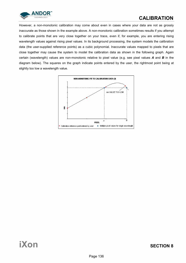
CALIBRATION
iXon SECTION 8
Page 136
However, a non-monotonic calibration may come about even in cases where your data are not as grossly
inaccurate as those shown in the example above. A non-monotonic calibration sometimes results if you attempt
to calibrate points that are very close together on your trace, even if, for example, you are entering rising
wavelength values against rising pixel values. In its background processing, the system models the calibration
data (the user-supplied reference points) as a cubic polynomial. Inaccurate values mapped to pixels that are
close together may cause the system to model the calibration data as shown in the following graph. Again
certain (wavelength) values are non-monotonic relative to pixel value (e.g. see pixel values A and B in the
diagram below). The squares on the graph indicate points entered by the user, the rightmost point being at
slightly too low a wavelength value.
CALIBRATION
iXon SECTION 8
Page 137
8.2.2.3 - Too few points
A calibration error will also occur if you have entered, in the Manual X-Calibration dialog box, no data points,
or only one data point. As general rule to obtain a good quality calibration, use more than five reference points,
at regular intervals, across the full width of the CCD sensor.
8.2.2.4 - Undo
Click the Undo button to exit the Manual X-Calibration dialog box and to undo any calibrations that you have
performed since entering the dialog box.
8.2.2.5 - Close
Click the Close button to exit the Manual X-Calibration dialog box.

CALIBRATION
iXon SECTION 8
Page 138
8.3 - X-CALIBRATION BY SPECTROGRAPH
To calibrate data using the spectrograph, select the X-Calibration by Spectrograph option from the
Calibration Menu. The Spectrograph X-Calibration dialog box will appear e.g.:
NOTE: The dialog box can also be opened by selecting the Setup Spectrograph option from the
Hardware menu on the Main Window.
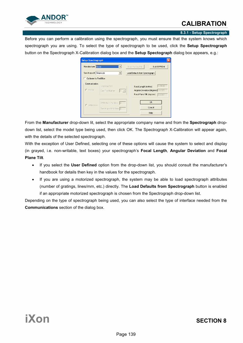
CALIBRATION
iXon SECTION 8
Page 139
8.3.1 - Setup Spectrograph
Before you can perform a calibration using the spectrograph, you must ensure that the system knows which
spectrograph you are using. To select the type of spectrograph to be used, click the Setup Spectrograph
button on the Spectrograph X-Calibration dialog box and the Setup Spectograph dialog box appears, e.g.:
From the Manufacturer drop-down lit, select the appropriate company name and from the Spectrograph drop-
down list, select the model type being used, then click OK. The Spectrograph X-Calibration will appear again,
with the details of the selected spectrograph.
With the exception of User Defined, selecting one of these options will cause the system to select and display
(in grayed, i.e. non-writable, text boxes) your spectrograph’s Focal Length, Angular Deviation and Focal
Plane Tilt.
• If you select the User Defined option from the drop-down list, you should consult the manufacturer’s
handbook for details then key in the values for the spectrograph.
• If you are using a motorized spectrograph, the system may be able to load spectrograph attributes
(number of gratings, lines/mm, etc.) directly. The Load Defaults from Spectrograph button is enabled
if an appropriate motorized spectrograph is chosen from the Spectrograph drop-down list.
Depending on the type of spectrograph being used, you can also select the type of interface needed from the
Communications section of the dialog box.
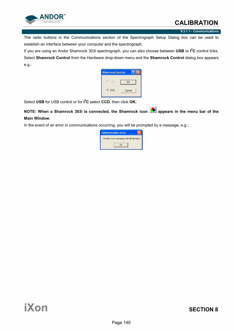
CALIBRATION
iXon SECTION 8
Page 140
8.3.1.1 - Communications
The radio buttons in the Communications section of the Spectrograph Setup Dialog box can be used to
establish an interface between your computer and the spectrograph.
If you are using an Andor Shamrock 303i spectrograph, you can also choose between USB or I2C control links.
Select Shamrock Control from the Hardware drop-down menu and the Shamrock Control dialog box appears
e.g.:
Select USB for USB control or for I2C select CCD, then click OK.
NOTE: When a Shamrock 303i is connected, the Shamrock icon appears in the menu bar of the
Main Window.
In the event of an error in communications occurring, you will be prompted by a message, e.g.:
CALIBRATION
iXon SECTION 8
Page 141
8.3.1.2 - Other spectographs
If you have selected an Oriel MS257 spectrograph for example, you can now Load Factory File. This file
supplies the system with important configuration details of your particular spectrograph. It must be loaded for the
system to control the spectrograph correctly. The Factory File will have been supplied on diskette with your
MS257 spectrograph. Performing Load Factory File lets you save the file contents to the .ini file included with
Andor’s software. The Factory File need not be loaded again.
When you click the Load Factory File button you will see a typical Windows ‘Open File’ dialog box. Select the
directory and the filename of the file you wish to load, and click OK. The Factory File is now loaded.
8.3.1.3 - Reverse spectrum
Some spectrographs produce somewhat ‘atypical’ spectra, where longer wavelengths (red) are to the left (as
viewed from the detector), and shorter wavelengths (blue) are to the right. If you select the MS127 or the FICS
spectrograph from the drop-down list for example, you will notice a tick in a Reverse Spectrum check box.
Because both these spectrographs are of this type, the Reverse Spectrum check box is ticked by default when
these spectrographs are selected. The system then uses software to ‘reverse’ the output of the detector when it
generates a data window, presenting the display in the more usual orientation. You may, if you wish, disable the
Reverse Spectrum function by clicking the check box.
8.3.1.4 - X-Axis label & units
The Spectrograph X-Calibration Dialog box allows you to select, from scrollable drop-down list boxes, an X-Axis
Label for your data window and an appropriate Unit of measurement. The following label & unit combinations
are available:
X-Axis Label Units
Wavelength nm, µm, cm-1
, eV
Raman Shift cm-1
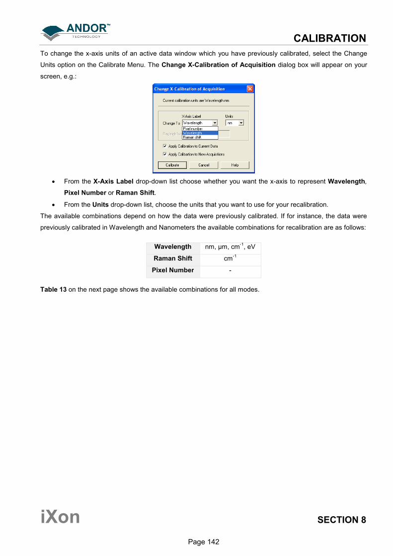
CALIBRATION
iXon SECTION 8
Page 142
To change the x-axis units of an active data window which you have previously calibrated, select the Change
Units option on the Calibrate Menu. The Change X-Calibration of Acquisition dialog box will appear on your
screen, e.g.:
• From the X-Axis Label drop-down list choose whether you want the x-axis to represent Wavelength,
Pixel Number or Raman Shift.
• From the Units drop-down list, choose the units that you want to use for your recalibration.
The available combinations depend on how the data were previously calibrated. If for instance, the data were
previously calibrated in Wavelength and Nanometers the available combinations for recalibration are as follows:
Wavelength nm, µm, cm-1
, eV
Raman Shift cm-1
Pixel Number -
Table 13 on the next page shows the available combinations for all modes.
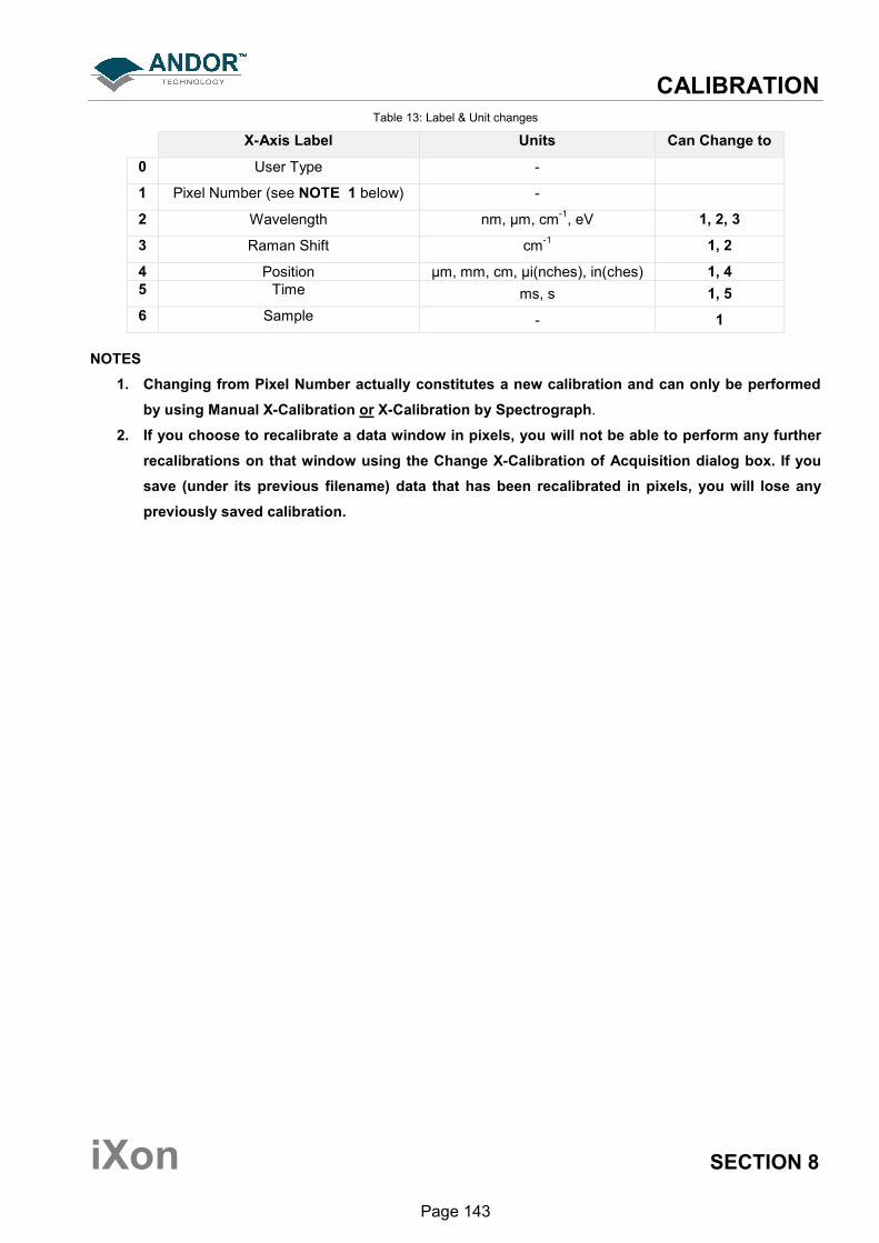
CALIBRATION
iXon SECTION 8
Page 143
Table 13: Label & Unit changes
X-Axis Label Units Can Change to
0 User Type -
1 Pixel Number (see NOTE 1 below) -
2 Wavelength nm, µm, cm-1
, eV 1, 2, 3
3 Raman Shift cm-1
1, 2
4 Position µm, mm, cm, µi(nches), in(ches) 1, 4
5 Time ms, s 1, 5
6 Sample - 1
NOTES
1. Changing from Pixel Number actually constitutes a new calibration and can only be performed
by using Manual X-Calibration or X-Calibration by Spectrograph.
2. If you choose to recalibrate a data window in pixels, you will not be able to perform any further
recalibrations on that window using the Change X-Calibration of Acquisition dialog box. If you
save (under its previous filename) data that has been recalibrated in pixels, you will lose any
previously saved calibration.
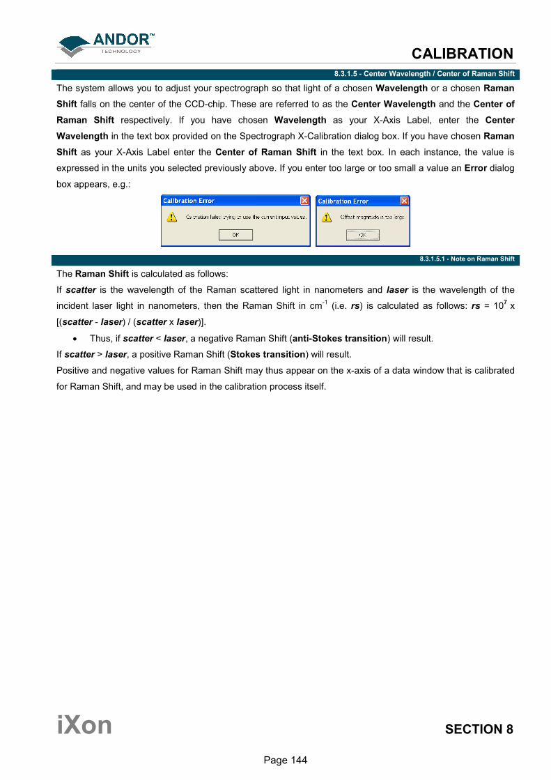
CALIBRATION
iXon SECTION 8
Page 144
8.3.1.5 - Center Wavelength / Center of Raman Shift
The system allows you to adjust your spectrograph so that light of a chosen Wavelength or a chosen Raman
Shift falls on the center of the CCD-chip. These are referred to as the Center Wavelength and the Center of
Raman Shift respectively. If you have chosen Wavelength as your X-Axis Label, enter the Center
Wavelength in the text box provided on the Spectrograph X-Calibration dialog box. If you have chosen Raman
Shift as your X-Axis Label enter the Center of Raman Shift in the text box. In each instance, the value is
expressed in the units you selected previously above. If you enter too large or too small a value an Error dialog
box appears, e.g.:
8.3.1.5.1 - Note on Raman Shift
The Raman Shift is calculated as follows:
If scatter is the wavelength of the Raman scattered light in nanometers and laser is the wavelength of the
incident laser light in nanometers, then the Raman Shift in cm-1
(i.e. rs) is calculated as follows: rs = 107
x
[(scatter - laser) / (scatter x laser)].
• Thus, if scatter < laser, a negative Raman Shift (anti-Stokes transition) will result.
If scatter > laser, a positive Raman Shift (Stokes transition) will result.
Positive and negative values for Raman Shift may thus appear on the x-axis of a data window that is calibrated
for Raman Shift, and may be used in the calibration process itself.

CALIBRATION
iXon SECTION 8
Page 145
8.3.1.6 - Offset
By entering a value in the Offset text box of the Spectrograph X-Calibration dialog box you can compensate for
small misalignments of the detector or the wavelength drive in your spectrograph. A positive value will cause
the x-axis of the data window to move to the right (relative to the trace) by the corresponding number of pixels.
A negative value will cause the x-axis to move to the left.
NOTE: To assess the accuracy of any calibration you have performed, you will need a calibration
spectral line source, such as a helium neon laser or a mercury vapor lamp. Ideally, set the spectrograph
to one of the prominent spectral lines, take a scan, and use the cursor on the data window to determine
any offset (in pixels) of the line from its true wavelength.
8.3.1.7 - Rayleigh Wavelength
If you have selected Raman Shift as your X-Axis Label, you must enter a value in nanometers for the Rayleigh
Wavelength. In Raman Spectroscopy the Rayleigh Wavelength is that element of a spectrum line (in scattered
radiation) whose wavelength is equal to that of the incident radiation (i.e. the laser wavelength) and is a product
of ordinary or Rayleigh scattering.
An error message will appear if you attempt to perform a calibration without having entered a valid Rayleigh
Wavelength, e.g.:

CALIBRATION
iXon SECTION 8
Page 146
8.3.1.8 - Micrometer setting
For certain non-motorized spectrographs, the system will calculate a Micrometer Setting that corresponds to
the Grating and the Center Wavelength / Center of Raman Shift you have chosen. The Micrometer Setting
allows you to manually adjust the angle of the diffraction grating (by means of the micrometer on the
spectrograph housing), so that light of the wavelength / Raman shift of your choice falls on the centre of the
CCD-chip. The Micrometer Setting appears in a text box on the Spectrograph X-Calibration dialog box. You
should use this value to manually set the micrometer on the spectrograph.
NOTE: If you choose to enter a micrometer setting, the system will calculate a value for the Center
Wavelength / Center of Raman Shift and vice versa. You need enter only one of the two values.
Because Raman shift does not correlate linearly with wavelength (or pixel positions), the center column of pixels
on the CCD-chip (e.g. column 800 on a chip of 1600 pixels width) is likely to be represented off-center on the x-
axis of a data window linearly calibrated for Raman shift. Column and where appropriate, row number, are
expressed in the form [x,y] on the status bar along the bottom edge of the data window.
NOTES:
1. If you choose Raman Shift as the X-Axis label, the Center Wavelength text box is relabeled
Center of Raman Shift.
2. In the case of motorized spectrographs, the wavelength drive is under direct software control.
8.3.1.9 - Grating
From the scrollable drop-down list select the specification of the diffraction grating you are currently using.
Grating specifications are shown as a line density followed by (where applicable) a blaze wavelength.
8.3.1.10 - Close
To exit the Spectrograph X-Calibration dialog box, click Close.
NOTE: The details you supply regarding your spectrograph, including any retrieved data will appear by
default whenever you open the Spectrograph X-Calibration dialog box subsequently. You can change
them whenever you choose.

CALIBRATION
iXon SECTION 8
Page 147
8.4 - PROCESSING DATA VIA THE COMMAND LINE
8.4.1 - Command Line
The Command Line allows you to enter one-line commands that are written in the Andor Basic programming
language. These commands are used to manipulate acquired data. Several command lines can be entered and
they are separated by “:”.
The open the Command Line dialog box, either click the button or select the Command Line option from
the Command drop-down menu. The dialog box opens, e.g.:
To run a command, click Execute. For further details of how to use the Andor Basic programming language,
please refer to the User’s Guide to Andor Basic.
8.4.2 - Calculations & Configure Calculations
• The Calculations option lets display the output of colorimetry calculations in a CIE Calculations
Window.
• The Configure Calculations option lets you choose which colorimetry calculations you are going to
perform and which parameters you are going to use.
For further information, please refer to Colorimetry Calculations in the Andor Radiometry Guide.
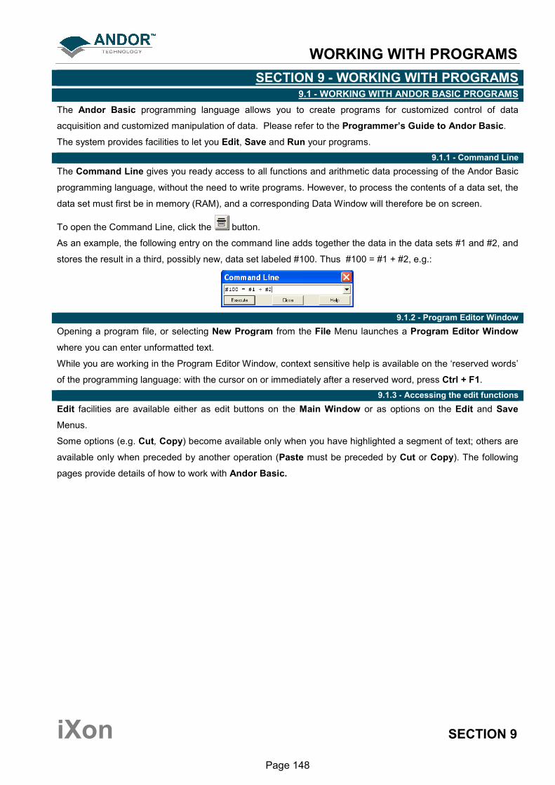
WORKING WITH PROGRAMS
iXon SECTION 9
Page 148
SECTION 9 - WORKING WITH PROGRAMS 9.1 - WORKING WITH ANDOR BASIC PROGRAMS
The Andor Basic programming language allows you to create programs for customized control of data
acquisition and customized manipulation of data. Please refer to the Programmer’s Guide to Andor Basic.
The system provides facilities to let you Edit, Save and Run your programs.
9.1.1 - Command Line
The Command Line gives you ready access to all functions and arithmetic data processing of the Andor Basic
programming language, without the need to write programs. However, to process the contents of a data set, the
data set must first be in memory (RAM), and a corresponding Data Window will therefore be on screen.
To open the Command Line, click the button.
As an example, the following entry on the command line adds together the data in the data sets #1 and #2, and
stores the result in a third, possibly new, data set labeled #100. Thus #100 = #1 + #2, e.g.:
9.1.2 - Program Editor Window
Opening a program file, or selecting New Program from the File Menu launches a Program Editor Window
where you can enter unformatted text.
While you are working in the Program Editor Window, context sensitive help is available on the ‘reserved words’
of the programming language: with the cursor on or immediately after a reserved word, press Ctrl + F1.
9.1.3 - Accessing the edit functions
Edit facilities are available either as edit buttons on the Main Window or as options on the Edit and Save
Menus.
Some options (e.g. Cut, Copy) become available only when you have highlighted a segment of text; others are
available only when preceded by another operation (Paste must be preceded by Cut or Copy). The following
pages provide details of how to work with Andor Basic.
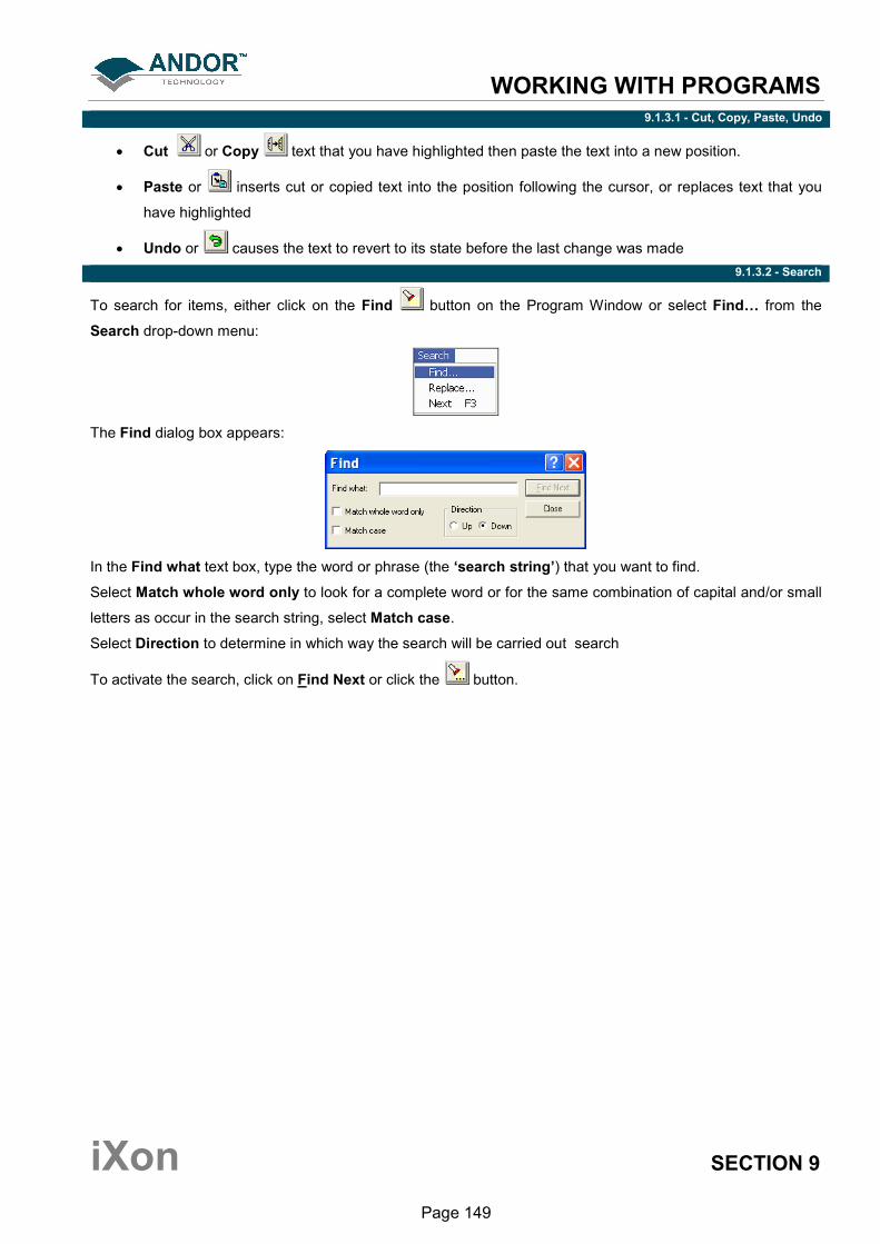
WORKING WITH PROGRAMS
iXon SECTION 9
Page 149
9.1.3.1 - Cut, Copy, Paste, Undo
• Cut or Copy text that you have highlighted then paste the text into a new position.
• Paste or inserts cut or copied text into the position following the cursor, or replaces text that you
have highlighted
• Undo or causes the text to revert to its state before the last change was made
9.1.3.2 - Search
To search for items, either click on the Find button on the Program Window or select Find… from the
Search drop-down menu:
The Find dialog box appears:
In the Find what text box, type the word or phrase (the ‘search string’) that you want to find.
Select Match whole word only to look for a complete word or for the same combination of capital and/or small
letters as occur in the search string, select Match case.
Select Direction to determine in which way the search will be carried out search
To activate the search, click on Find Next or click the button.
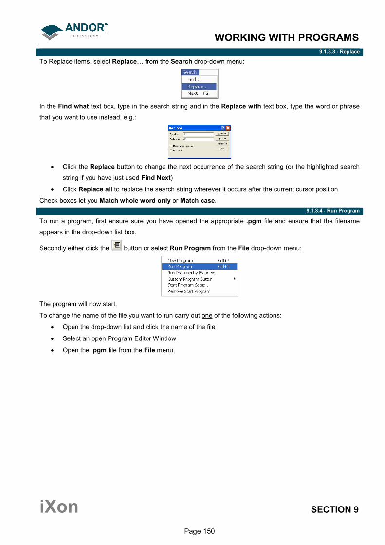
WORKING WITH PROGRAMS
iXon SECTION 9
Page 150
9.1.3.3 - Replace
To Replace items, select Replace… from the Search drop-down menu:
In the Find what text box, type in the search string and in the Replace with text box, type the word or phrase
that you want to use instead, e.g.:
• Click the Replace button to change the next occurrence of the search string (or the highlighted search
string if you have just used Find Next)
• Click Replace all to replace the search string wherever it occurs after the current cursor position
Check boxes let you Match whole word only or Match case.
9.1.3.4 - Run Program
To run a program, first ensure sure you have opened the appropriate .pgm file and ensure that the filename
appears in the drop-down list box.
Secondly either click the button or select Run Program from the File drop-down menu:
The program will now start.
To change the name of the file you want to run carry out one of the following actions:
• Open the drop-down list and click the name of the file
• Select an open Program Editor Window
• Open the .pgm file from the File menu.

WORKING WITH PROGRAMS
iXon SECTION 9
Page 151
9.1.3.5 - Run Program by Filename
You may also run a program by means of the Run Program by Filename option on the File Menu. Select Run
Program by Filename from the File drop-down menu:
A standard Open dialog box appears, from which you may select the file whose contents you want to run. The
file containing the program appears on screen as an iconized Program Editor Window and the program
begins to execute immediately.
9.1.3.6 - Entering program input
Any text-based input required by the program (i.e. in Andor Basic you have indicated that the user must
manually enter a value at a particular point in the program’s execution) is entered via an Input dialog box.

APPENDIX
iXon APPENDIX
Page 152
APPENDIX A1 - GLOSSARY
If this is the first time you have used Andor’s EMCCD, the glossary that follows will help familiarize you with its
design philosophy and some of its key terminology.
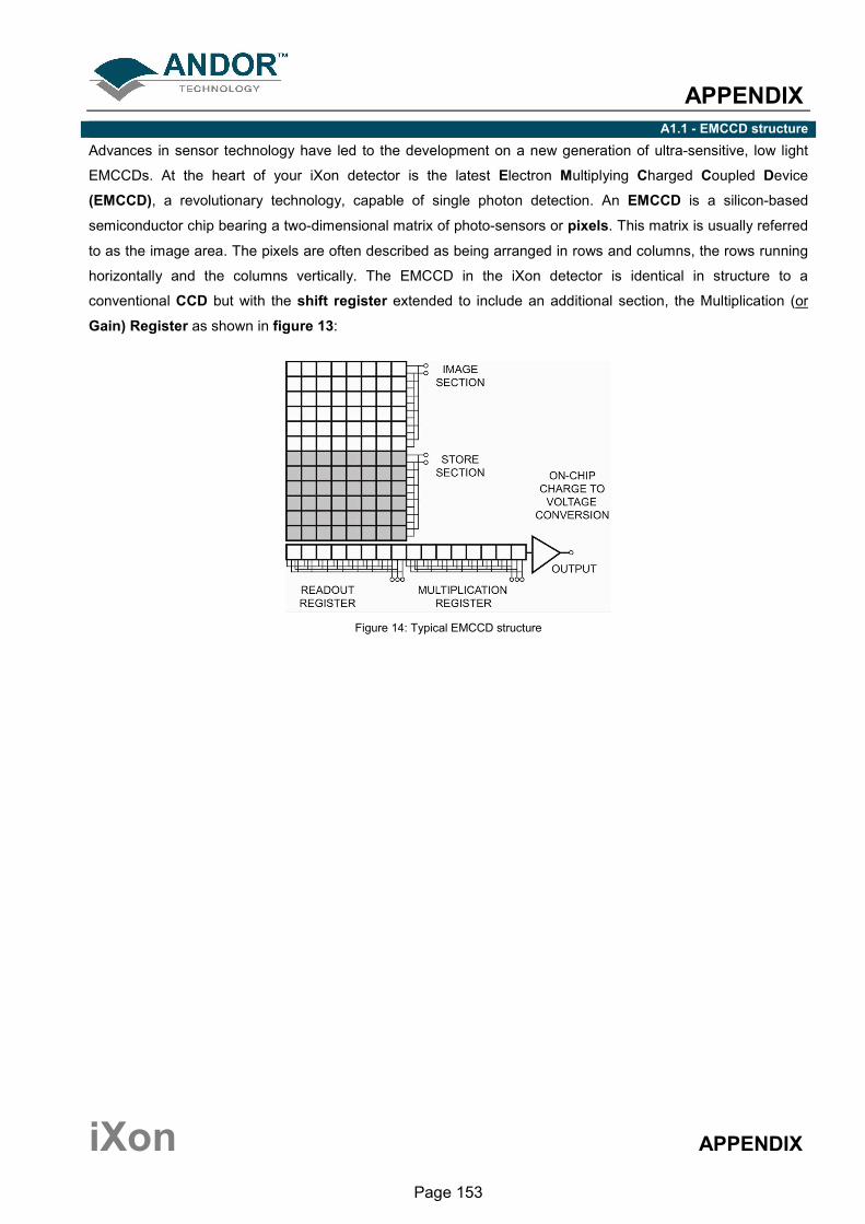
APPENDIX
iXon APPENDIX
Page 153
A1.1 - EMCCD structure
Advances in sensor technology have led to the development on a new generation of ultra-sensitive, low light
EMCCDs. At the heart of your iXon detector is the latest Electron Multiplying Charged Coupled Device
(EMCCD), a revolutionary technology, capable of single photon detection. An EMCCD is a silicon-based
semiconductor chip bearing a two-dimensional matrix of photo-sensors or pixels. This matrix is usually referred
to as the image area. The pixels are often described as being arranged in rows and columns, the rows running
horizontally and the columns vertically. The EMCCD in the iXon detector is identical in structure to a
conventional CCD but with the shift register extended to include an additional section, the Multiplication (or
Gain) Register as shown in figure 13:
Figure 14: Typical EMCCD structure
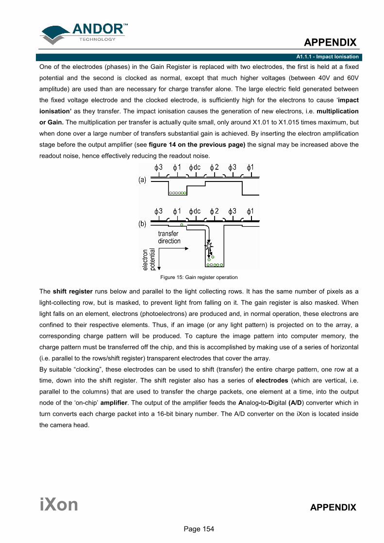
APPENDIX
iXon APPENDIX
Page 154
A1.1.1 - Impact Ionisation
One of the electrodes (phases) in the Gain Register is replaced with two electrodes, the first is held at a fixed
potential and the second is clocked as normal, except that much higher voltages (between 40V and 60V
amplitude) are used than are necessary for charge transfer alone. The large electric field generated between
the fixed voltage electrode and the clocked electrode, is sufficiently high for the electrons to cause ‘impact
ionisation’ as they transfer. The impact ionisation causes the generation of new electrons, i.e. multiplication
or Gain. The multiplication per transfer is actually quite small, only around X1.01 to X1.015 times maximum, but
when done over a large number of transfers substantial gain is achieved. By inserting the electron amplification
stage before the output amplifier (see figure 14 on the previous page) the signal may be increased above the
readout noise, hence effectively reducing the readout noise.
Figure 15: Gain register operation
The shift register runs below and parallel to the light collecting rows. It has the same number of pixels as a
light-collecting row, but is masked, to prevent light from falling on it. The gain register is also masked. When
light falls on an element, electrons (photoelectrons) are produced and, in normal operation, these electrons are
confined to their respective elements. Thus, if an image (or any light pattern) is projected on to the array, a
corresponding charge pattern will be produced. To capture the image pattern into computer memory, the
charge pattern must be transferred off the chip, and this is accomplished by making use of a series of horizontal
(i.e. parallel to the rows/shift register) transparent electrodes that cover the array.
By suitable “clocking”, these electrodes can be used to shift (transfer) the entire charge pattern, one row at a
time, down into the shift register. The shift register also has a series of electrodes (which are vertical, i.e.
parallel to the columns) that are used to transfer the charge packets, one element at a time, into the output
node of the ‘on-chip’ amplifier. The output of the amplifier feeds the Analog-to-Digital (A/D) converter which in
turn converts each charge packet into a 16-bit binary number. The A/D converter on the iXon is located inside
the camera head.

APPENDIX
iXon APPENDIX
Page 155
A1.1.2 - EMCCD readout sequence
In the course of readout, charge is moved vertically into the shift register, and then horizontally from the shift
register into the output node of the amplifier. The simple readout sequence illustrated below (which corresponds
to the default setting of the Full Resolution Image binning pattern) allows data to be recorded for each
individual element on the EMCCD-chip.
Other binning patterns are achieved by summing charge in the shift register and/or the output node prior to
readout. Please see Vertical & Horizontal Binning on pages 157 - 158.
1 Exposure to light causes a pattern of charge (an electronic image) to build up on the frame (or Image
Area) of the EMCCD-chip.
2 Charge in the frame is shifted vertically by one row, so that the bottom row of charge moves into the shift
register.
3 Charge in the shift register is moved horizontally by one pixel, so that charge on the endmost pixel of the
shift register is moved into the Gain register.
4 Charge is shifted into the output node of the amplifier.
5 The charge in the output node of the amplifier is passed to the analog-to-digital converter and is read out.
6 Steps 3 and 4 are repeated until the shift register is emptied of charge.
7 The frame is shifted vertically again, so that the next row of charge moves down into the shift register.
The process is repeated from Step 3 until the whole frame is read out.
APPENDIX
iXon APPENDIX
Page 156
A1.2 - Accumulation
Accumulation is the process by which data that have been acquired from a number of similar scans are added
together in computer memory. This results in improved signal to noise ratio.
A1.3 - Acquisition
An Acquisition is taken to be the complete data capture process.
A1.4 - A/D Conversion
Charge from the CCD is initially read as an analog signal, ranging from zero to the saturation value. A/D
conversion changes the analog signal to a binary number which can then be manipulated by the computer.
A1.5 - Background
Background is a data acquisition made in darkness. It is made up of fixed pattern noise, and any signal due to
dark current.
A1.6 - Binning
Binning is a process that allows charge from two or more pixels to be combined on the EMCCD-chip prior to
readout (please refer to EMCCD Readout Sequence on the previous page.)
Summing charge on the EMCCD and performing a single readout gives better noise performance than reading
out several pixels and then summing them in the computer memory. This is because each act of reading out
contributes to noise. There are two main variants of the binning process as follows:
• Vertical binning
• Horizontal binning
In addition there are several binning patterns that tailor the main binning variants to typical application usage.

APPENDIX
iXon APPENDIX
Page 157
A1.6.1 - Vertical Binning
In Vertical Binning, charge from two or more rows of the EMCCD-chip is moved down into the shift register
before the charge is read out. The number of rows shifted depends on the binning pattern you have selected.
Thus, for each column of the EMCCD-chip, charge from two or more vertical elements is summed into the
corresponding element of the shift register. The charge from each of the pixels in the shift register is then
shifted horizontally to the output node of the amplifier and read out. The figure below illustrates readout of data
from adjacent tracks, each track comprising two binned rows of the EMCCD-chip:
1 Exposure to light causes a pattern of charge (an electronic image) to build up on the frame (or “image
area”) of the EMCCD-chip.
2 Charge in the frame is shifted vertically by one row, so that the bottom row of charge moves down into
the shift register.
3 Charge in the frame is shifted vertically by a further row, so that the next row of charge moves down into
the shift register, which now contains charge from two rows - i.e. the charge is vertically binned.
4 Charge in the shift register is moved horizontally by one pixel, so that charge on the endmost pixel of the
shift register is moved into the Gain Register
5 Charge is shifted into the output node of the amplifier
6 The charge in the output node of the amplifier is passed to the analog-to-digital converter and is read out
Steps 4 and 5 are repeated until the shift register is empty. The process is repeated from Step 2 until the
whole frame is read out

APPENDIX
iXon APPENDIX
Page 158
A1.6.2 - Horizontal Binning (creating Superpixels)
Shifting the charge horizontally from several pixels at a time into the output node is known as Horizontal
Binning. Horizontal binning in combination with Vertical binning allows you to define so-called superpixels
that in Image Display Mode represent as a single picture element charge that has been binned from a group of
pixels. For example, charge that is binned vertically from two rows and horizontally from two pixels before
being read out is displayed as a superpixel of dimensions 2x2 pixels. You can define these superpixels from
the Imaging Dialog Box. On the one hand, superpixels (by comparison with single pixels) result in a more
coarsely defined image when the data are displayed in Image Display Mode. On the other hand, superpixels
offer the advantages of summing data on-chip prior to readout.
In the example below, where each superpixel is of dimensions 2x2 pixels, charge from two rows is first binned
vertically into the shift register. Charge from two pixels of the shift register is then binned horizontally into the
output node of the amplifier. The effect of the combined binning processes is a summed charge equating to a
2x2 “superpixel”. Since this example initially involves binning charge from two rows, the process begins in the
same way as Steps 1 - 4 of Vertical Binning of Two Rows on page 157), then horizontal binning begins.
…4 Charge from two rows has already been vertically binned into the shift register (see Vertical Binning
of Two Rows on the previous page). Now charge in the shift register is moved horizontally by one
pixel, so that charge on the endmost pixel of the shift register is moved into the Gain Register, and
subsequently into the output node of the amplifier.)
5 Charge in the shift register is again moved horizontally, so that the output node of the amplifier now
contains charge from two pixels of the shift register - i.e. the charge has been horizontally binned.
6 The charge in the output node of the amplifier is passed to the analog-to-digital converter and is re see
ad out.
7 Steps 4 to 6 are repeated until the shift register is empty. The process is repeated from Step 2 (again
please see Vertical Binning of Two Rows on the previous page) until the whole frame is read out.
APPENDIX
iXon APPENDIX
Page 159
A1.7 - Counts
Counts refer to the digitization by the A/D conversion and are the basic unit in which data are displayed and
processed. Depending on the particular version of the detection device, one count may, for example, be
equated with a charge of 10 photoelectrons on a pixel of the CCD.
A1.8 - Dark Signal
Dark signal, a charge usually expressed as a number of electrons, is produced by the flow of dark current
during the exposure time. All CCD’s produce a dark current, an actual current that is measurable in (typically
tenths of) milliamps per pixel. The dark signal adds to your measured signal level, and increases the amount of
noise in the measured signal. Since the dark signal varies with temperature, it can cause background values to
increase over time. It also sets a limit on the useful exposure time.
Reducing the temperature of the CCD reduces dark signal (typically, for every 7ºC that temperature falls, dark
signal halves). CCD readout noise is low, and so as not to compromise this by shot noise from the dark signal, it
is important to cool the detector to reduce the dark signal. If you are using an exposure time of less than a few
seconds, cooling the detector below 0ºC will generally remove most of the shot noise caused by dark signal.
A1.9 - Detection Limit
The Detection Limit is a measure of the smallest signal that can be detected in a single readout. The smallest
signal is defined as the signal whose level is equal to the noise accompanying that signal, i.e. a signal to noise
ratio (S/N) of unity. Sources of noise are:
• Shot noise of the signal itself
• Shot noise of any dark signal
• Readout noise
If the signal is small, we can ignore its shot noise.
Furthermore, if a suitably low operating temperature and short exposure time can be achieved, the lowest
detection limit will equal the readout noise.
A1.10 - Exposure Time
The Exposure Time is the period during which the CCD collects light prior to readout.
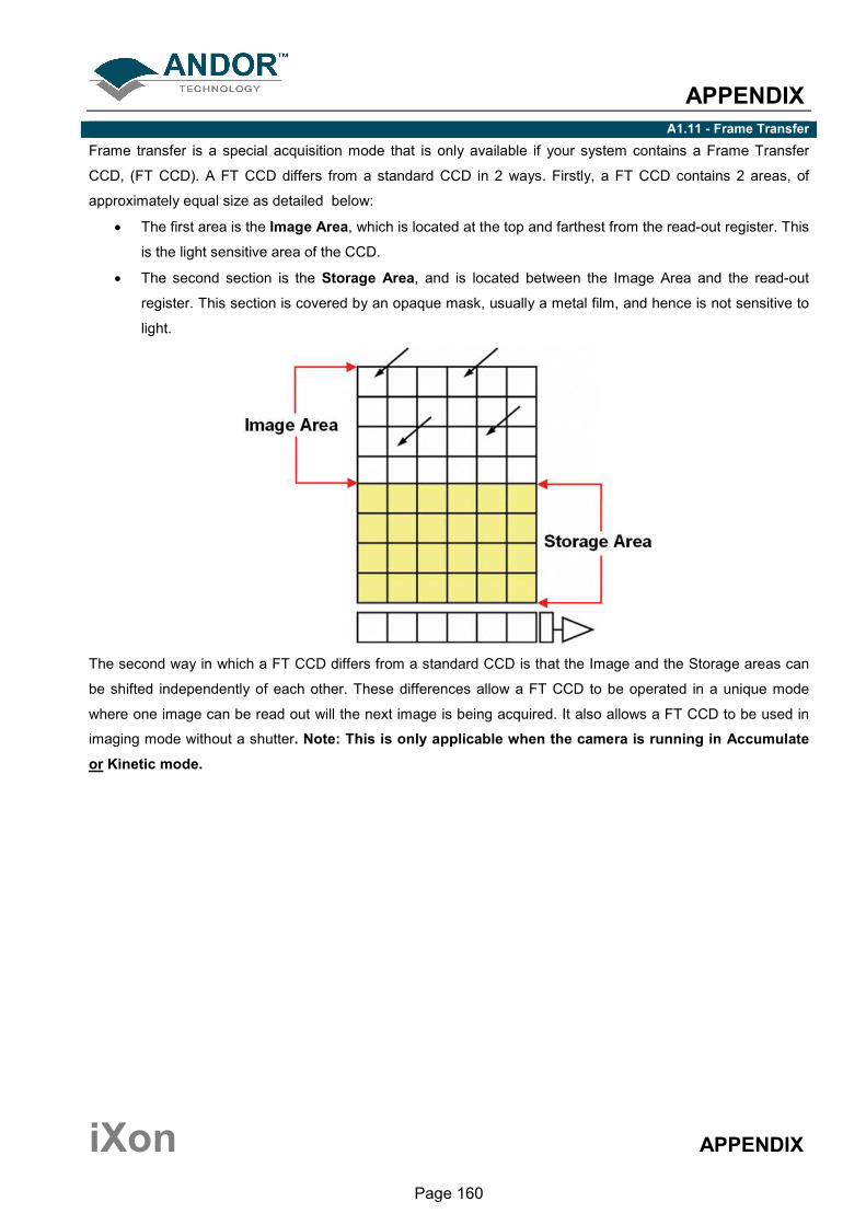
APPENDIX
iXon APPENDIX
Page 160
A1.11 - Frame Transfer Frame transfer is a special acquisition mode that is only available if your system contains a Frame Transfer
CCD, (FT CCD). A FT CCD differs from a standard CCD in 2 ways. Firstly, a FT CCD contains 2 areas, of
approximately equal size as detailed below:
• The first area is the Image Area, which is located at the top and farthest from the read-out register. This
is the light sensitive area of the CCD.
• The second section is the Storage Area, and is located between the Image Area and the read-out
register. This section is covered by an opaque mask, usually a metal film, and hence is not sensitive to
light.
The second way in which a FT CCD differs from a standard CCD is that the Image and the Storage areas can
be shifted independently of each other. These differences allow a FT CCD to be operated in a unique mode
where one image can be read out will the next image is being acquired. It also allows a FT CCD to be used in
imaging mode without a shutter. Note: This is only applicable when the camera is running in Accumulate
or Kinetic mode.
APPENDIX
iXon APPENDIX
Page 161
A1.12 - Gain
A1.12.1 - Gain and Dynamic Range As the gain is increased it will at some point begin to cause a decrease in Dynamic Range. This occurs when
the gain equals the readout noise, in electrons. Therefore at 1MHz readout rates the Dynamic Range will be
maintained at over 20,000:1 for gains up to about 20 times, while at 62.5kHz it will be maintained at over
43,000:1 for gains up to 6 times.
If higher sensitivities (and hence higher gains) are required then, there will have to be a trade off for Dynamic
Range. To maintain as much Dynamic Range as possible it is advisable not to use a higher gain than is
necessary to measure a signal.
A1.12.2 - Gain and noise The output from the gain register is fed into a conventional CCD output amplifier. This amplifier, even in a
scientific CCD, will have a readout noise of a few electrons rms and around 10 or 20 electrons rms at MHz
readout rates. However this noise will effectively be reduced by the multiplication factor of the gain register
which, when high enough, will achieve noise levels below 1 electron rms. So by using the gain you can
effectively reduce the noise to insignificant levels at any readout speed. For example, the iXon 87 has an s
readout noise of a few to tens of electrons, depending on read out speed.
Using gain will itself add some noise to a measured signal due to the statistical nature of the multiplication
process. A similar effect exists in ICCDs and is referred to as the Noise Factor. The amount added is dependent
on the signal level and the gain. If there is no gain, then there is no extra noise. At high gain (tens of times
higher) it is calculated as the square root of N (where N is the signal in electrons). This will add to the shot noise
of the signal to become the square root of 2N. So if the signal is large enough to be above the readout noise
then there is probably no need for gain and it should be reduced or turned off.
Conversely, if the signal is being lost in the readout noise then increasing the gain is the only way to detect it. If
the gain is set high enough, then detection of single electron events will be possible. These events will appear
on an image as a spike several hundred counts high. In Andor EMCCD cameras the gain is limited to a
maximum of 255 times @ -50ºC for standard systems. This is comparable to high end ICCDs.
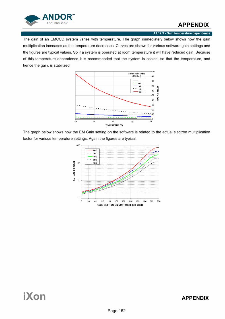
APPENDIX
iXon APPENDIX
Page 162
A1.12.3 - Gain temperature dependence
The gain of an EMCCD system varies with temperature. The graph immediately below shows how the gain
multiplication increases as the temperature decreases. Curves are shown for various software gain settings and
the figures are typical values. So if a system is operated at room temperature it will have reduced gain. Because
of this temperature dependence it is recommended that the system is cooled, so that the temperature, and
hence the gain, is stabilized.
The graph below shows how the EM Gain setting on the software is related to the actual electron multiplication
factor for various temperature settings. Again the figures are typical.

APPENDIX
iXon APPENDIX
Page 163
A1.13- Keep Cleans
The CCD-chip is continually being scanned to prevent its becoming saturated with dark current. Scanning
involves moving charge from the CCD-chip into the shift register and then emptying the shift register. If the scan
is being used simply to clean the CCD-chip (i.e. it is a keep-clean scan), the charge that is emptied from the
shift register is not stored in memory and is, in effect, discarded.
While running an Accumulate or Kinetic acquisition, use the Keep Clean Dialogue box to enter a minimum
number of Keep Cleans between each scan in the series.
APPENDIX
iXon APPENDIX
Page 164
A1.14 - Noise
Noise is a complex topic, the full exploration of which is beyond the scope of this glossary. However noise may
be broken down into two broad categories, as follows:
• Pixel Noise
• Fixed Pattern Noise
A1.14.1 - Pixel noise
Let us first attempt to define pixel noise. Assume that a light signal is falling on a pixel of the CCD. If the charge
on the pixel is read, and the read process is repeated many times, the noise may be taken as the variation in
the values read. The Root Mean Square (r.m.s.) of these variations is often used to express a value for noise.
As a rule of thumb, the r.m.s. is four to six times smaller than the peak to peak variations in the count values
read from the pixel. Pixel noise has three main constituents:
• Readout noise
• Shot noise from the dark signal
• Shot noise from the light signal itself
Shot noise cannot be removed because it is due to basic physical laws. Most simply defined, shot noise is the
square root of the signal (or dark signal) measured in electrons.
A1.14.2 - Fixed Pattern noise
Fixed Pattern Noise (FPN) consists of the differences in count values read out from individual pixels, even if no
light is falling on the detector. These differences remain constant from read to read. The differences are due in
part to a variation in the dark signal produced by each pixel, and in part to small irregularities that arise during
the fabrication of the CCD. Since fixed pattern noise is partly due to dark signal, it will change if the temperature
changes, but because it is fixed, it can be completely removed from a measurement by background subtraction.
A1.14.3 - Readout noise
Readout noise (which in our detectors is, in any case, low) is due to the amplifier and electronics: it is
independent of dark signal and signal levels; it is only very slightly dependent on temperature; and it is present
on every read, as a result of which it sets a limit on the best achievable noise performance.
Shot noise from the dark signal is dependent on the exposure time and is very dependent on the temperature;
shot noise from the signal is additionally dependent on the signal level itself. If either the signal or the dark
signal falls to zero, their respective shot noise also falls to zero.
The total pixel noise is not, however, simply the sum of the three main noise components (readout noise, shot
noise from the dark signal, and shot noise from the signal). Rather, the Root Sum Square (r.s.s.) gives a
reasonable approximation - thus:
total = sqrt (readnoise² + darkshot² + sigshot²)
where:
• total is the pixel noise
• readnoise is the readout noise
• darkshot is the shot noise of the dark signal
• sigshot is the shot noise of the signal
APPENDIX
iXon APPENDIX
Page 165
A1.15 - Quantum Efficiency/Spectral Response
The glossary refers to signals as a number of electrons. More strictly speaking these are ‘photoelectrons’,
created when a photon is absorbed. When a UV or visible photon is absorbed by the detector it can at best
produce only one photoelectron. Photons of different wavelengths have different probabilities of producing a
photoelectron and this probability is usually expressed as Quantum Efficiency (QE) or spectral response.
QE is a percentage measure of the probability of a single photon producing a photoelectron, while spectral
response is the number of electrons that will be produced per unit photon energy. Many factors contribute to
the QE of a CCD, but the most significant factor is the absorption coefficient of the silicon that serves as the
bulk material of the device
A1.16 - Readout
Readout is the process by which data are taken from the pixels of the CCD and stored in computer memory.
The pixels, which are arranged in a single row, are read out individually in sequence. Readout involves
amplifying the charge on each pixel into a voltage, performing an A/D conversion, and storing the data in
computer memory. The time taken to perform this operation is known as the “read time”.
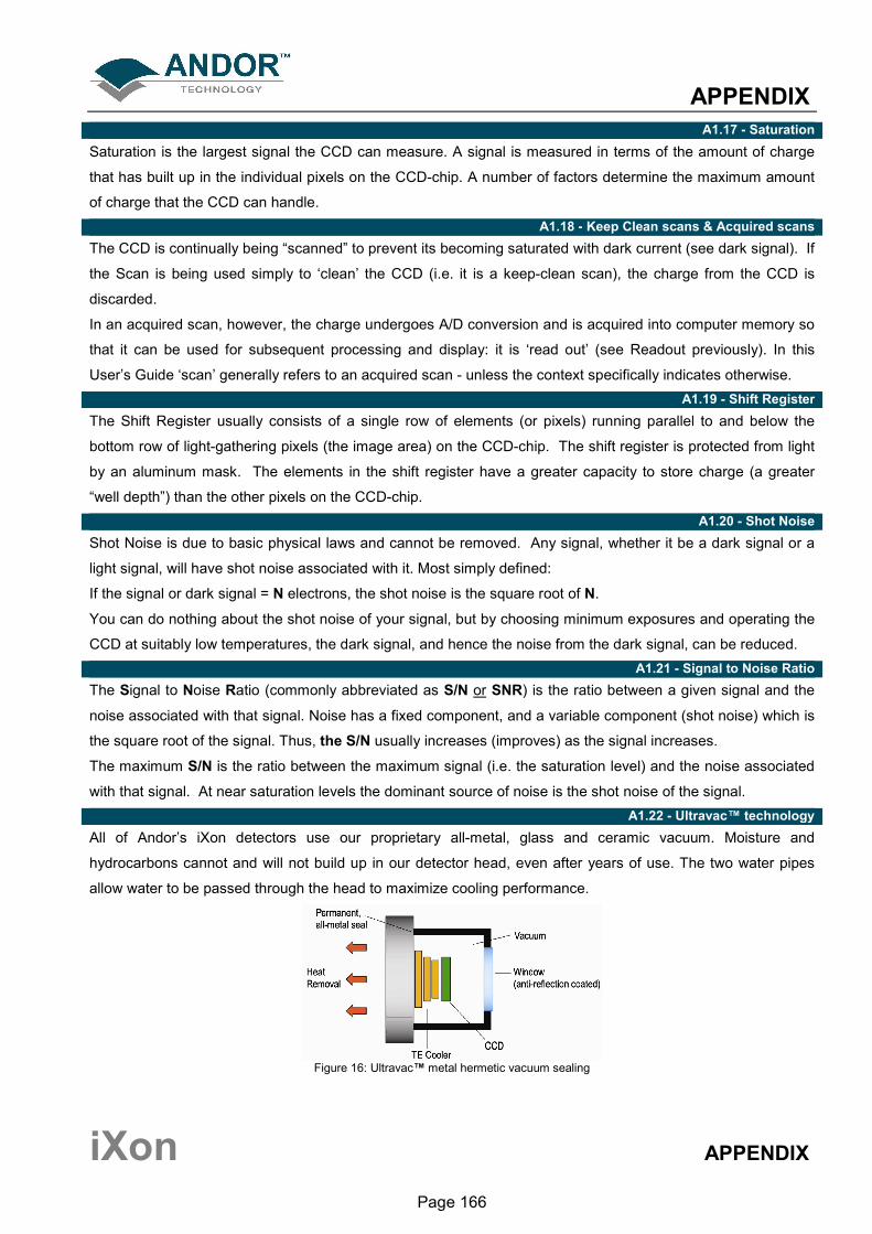
APPENDIX
iXon APPENDIX
Page 166
A1.17 - Saturation
Saturation is the largest signal the CCD can measure. A signal is measured in terms of the amount of charge
that has built up in the individual pixels on the CCD-chip. A number of factors determine the maximum amount
of charge that the CCD can handle.
A1.18 - Keep Clean scans & Acquired scans
The CCD is continually being “scanned” to prevent its becoming saturated with dark current (see dark signal). If
the Scan is being used simply to ‘clean’ the CCD (i.e. it is a keep-clean scan), the charge from the CCD is
discarded.
In an acquired scan, however, the charge undergoes A/D conversion and is acquired into computer memory so
that it can be used for subsequent processing and display: it is ‘read out’ (see Readout previously). In this
User’s Guide ‘scan’ generally refers to an acquired scan - unless the context specifically indicates otherwise.
A1.19 - Shift Register
The Shift Register usually consists of a single row of elements (or pixels) running parallel to and below the
bottom row of light-gathering pixels (the image area) on the CCD-chip. The shift register is protected from light
by an aluminum mask. The elements in the shift register have a greater capacity to store charge (a greater
“well depth”) than the other pixels on the CCD-chip.
A1.20 - Shot Noise
Shot Noise is due to basic physical laws and cannot be removed. Any signal, whether it be a dark signal or a
light signal, will have shot noise associated with it. Most simply defined:
If the signal or dark signal = N electrons, the shot noise is the square root of N.
You can do nothing about the shot noise of your signal, but by choosing minimum exposures and operating the
CCD at suitably low temperatures, the dark signal, and hence the noise from the dark signal, can be reduced.
A1.21 - Signal to Noise Ratio
The Signal to Noise Ratio (commonly abbreviated as S/N or SNR) is the ratio between a given signal and the
noise associated with that signal. Noise has a fixed component, and a variable component (shot noise) which is
the square root of the signal. Thus, the S/N usually increases (improves) as the signal increases.
The maximum S/N is the ratio between the maximum signal (i.e. the saturation level) and the noise associated
with that signal. At near saturation levels the dominant source of noise is the shot noise of the signal.
A1.22 - Ultravac™ technology
All of Andor’s iXon detectors use our proprietary all-metal, glass and ceramic vacuum. Moisture and
hydrocarbons cannot and will not build up in our detector head, even after years of use. The two water pipes
allow water to be passed through the head to maximize cooling performance.
Figure 16: Ultravac™ metal hermetic vacuum sealing
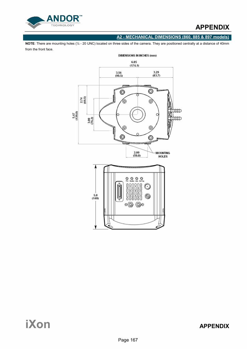
APPENDIX
iXon APPENDIX
Page 167
A2 - MECHANICAL DIMENSIONS (860, 885 & 897 models)
NOTE: There are mounting holes (¼ - 20 UNC) located on three sides of the camera. They are positioned centrally at a distance of 40mm
from the front face.
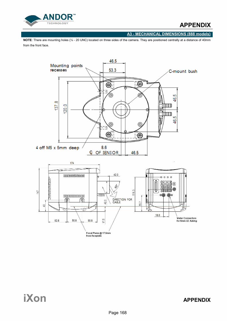
APPENDIX
iXon APPENDIX
Page 168
A3 - MECHANICAL DIMENSIONS (888 models)
NOTE: There are mounting holes (¼ - 20 UNC) located on three sides of the camera. They are positioned centrally at a distance of 40mm
from the front face.

APPENDIX
iXon APPENDIX
Page 169
A4 - TERMS & CONDITIONS
1. In these Conditions:
‘BUYER’ means the person who accepts a quotation of the Seller for the sale of the Goods or whose order
for the Goods is accepted by the Seller.
‘GOODS’ means the goods (including any instalment of the goods or any parts for them) which the Seller is
to supply in accordance with these Conditions.
‘SELLER’ means Andor Technology Limited.
‘CONDITIONS’ means the standard terms and conditions of sale set out in this document and (unless the
context otherwise requires) includes any special terms and conditions agreed in writing between the Buyer
and Seller.
‘CONTRACT’ means the contract for the purchase and sale of the Goods.
‘WRITING’ includes telex, cable, facsimile transmission and comparable means of communication.
2. Any reference in these Conditions to any provision of a statute shall be construed as a reference to that
provision as amended, re-enacted or extended at the relevant time.
3. The headings in these Conditions are for convenience only and shall not affect their interpretation.
APPENDIX
iXon APPENDIX
Page 170
A5 - WARRANTIES & LIABILITY
1. Subject to these Conditions set out below, the Seller warrants that the Goods will correspond with their
specification at the time of delivery and will be free from defects in material and workmanship for a period of 12
months from the date of delivery.
2. The above warranty is given by the Seller subject to the following conditions:
2.1 the Seller shall be under no liability in respect of any defect in the Goods arising from any drawing, design
or specifications supplied by the Buyer;
2.2 the Seller shall be under no liability in respect of any defect arising from fair wear and tear, wilful damage,
negligence, abnormal working conditions, failure to follow the Seller’s instructions (whether oral or in writing),
misuse or alteration or repair of the Goods without the Seller’s approval;
2.3 the Seller shall be under no liability under the above warranty (or other warranty, condition or guarantee) if
the total price for the Goods has not been paid by the due date for payment;
2.4 the above warranty does not extend to parts, material or equipment not manufactured by the Seller, in
respect of which the Buyer shall only be entitled to the benefit of any such warranty or guarantee as is given by
the manufacturer to the Seller.
3. Subject as expressly provided in these conditions, and except where the Goods are sold to a person dealing
as a consumer (within the meaning of the Unfair Contract Terms Act 1977), all warranties, conditions or other
terms implied by statute or common law are excluded to the fullest extent permitted by law.
4. Any claim by the Buyer which is based on any defect in the quality or condition of the Goods or their failure
to correspond with specification shall (whether or not delivery is refused by the Buyer) be notified in Writing to
the Seller within 7 days from the date of delivery or (where the defect or failure was not apparent on reasonable
inspection) discovery of the defect or failure. If delivery is not refused, and the Buyer does not notify the Seller
accordingly, the Buyer shall not be entitled to reject the Goods and the Seller shall have no liability for such
defect or failure, and the Buyer shall be bound to pay the price as if the Goods had been delivered in
accordance with the Contract. In no event shall the Buyer be entitled to reject the Goods on the basis of any
defect or failure which is so slight that it would be unreasonable for him to reject them.
APPENDIX
iXon APPENDIX
Page 171
5. Where any valid claim in respect of the Goods which is based on any defect in the quality or condition of the
Goods or their failure to meet specification is notified to the Seller in accordance with these Conditions, the
Seller shall be entitled to replace the Goods (or the part in question) free of charge or, at the Seller’s sole
discretion, refund to the Buyer the price of the Goods (or a proportionate part of the price), but the Seller shall
have no further liability to the Buyer.
6. Except in respect of death or personal injury caused by the Seller’s negligence, the Seller shall not be liable
to the Buyer by reason of any representation (unless fraudulent), or any implied warranty, condition or other
term, or any duty at common law, or under the express terms of the Contract, for any indirect, special or
consequential loss or damage (whether for loss of profit or otherwise), costs, expenses or other claims for
compensation whatsoever (whether caused by the negligence of the Seller, its employees or against otherwise)
which arise out of or in connection with the supply of the Goods, or their use or resale by the Buyer and the
entire liability of the Seller under or in connection with the Contract shall not exceed the price of the goods,
except as expressly provided in these Conditions.
7. The Seller shall not be liable to the Buyer or be deemed to be in breach of the Contract by reason of any
delay in performing, or any failure to perform, any of the Seller’s obligations in relation to the goods, if the delay
or failure was due to any cause beyond the Seller’s reasonable control. Without prejudice to the generality of
the foregoing, the following shall be regarded as causes beyond the Seller’s reasonable control:
7.1 Act of God, explosion, flood, tempest, fire or accident;
7.2 war or threat of war, sabotage, insurrection, civil disturbance or requisition;
7.3 acts, restrictions, regulations, bye-laws, prohibitions or measures of any kind on the part of any
governmental, parliamentary or local authority;
7.4 import or export regulations or embargoes;
7.5 strikes, lock-outs or other industrial actions or trade disputes (whether involving employees of the Seller or
of third party);
7.6 difficulties in obtaining raw materials, labour, fuel, parts or machinery;
7.7 power failure or breakdown in machinery.