itto pd 73/89 (f,m,i) phase ii feasibility study …puspijak.org/publikasi/buku ilmiah...
TRANSCRIPT
ISBN: 978-602-7672-14-7
9 786027 672147
Executing AgencyCenter for Research and Development on Climate Change and Policy Forestry Research and Development Agency (FORDA)
Starting date : 1 October 2011Duration : 6 (Six) months
Host Government Republic of Indonesia
ITTO PD 73/89 (F,M,I) Phase IIFEASIBILITY STUDY ON REDD+
IN CENTRAL KALIMANTAN INDONESIA
Methodology Design Document for Reducing Emissions from Deforestation and
Degradation of Undrained Peat Swamp Forests in Central Kalimantan, Indonesia
IT OT
STARLING RESOURCES
Erica Meta SmithSteven De Gryze
Jeff Silverman Rezal Kusumaatmadja
Taryono DarusmanMartin Hardiono
I Wayan Susi DharmawanSulistyo A. Siran
Virni Budi Arifanti
Executing AgencyCenter for Research and Development on Climate Change and Policy Forestry Research and Development Agency (FORDA)
Starting date : 1 October 2011Duration : 6 (Six) months
Host Government Republic of Indonesia
ITTO PD 73/89 (F,M,I) Phase IIFEASIBILITY STUDY ON REDD+
IN CENTRAL KALIMANTAN INDONESIA
Methodology Design Document for Reducing Emissions from Deforestation and Degradation of Undrained Peat Swamp Forests
in Central Kalimantan, Indonesia
IT OT
STARLING RESOURCES
Sulistyo A. SiranRumi Naito
I Wayan Susi DharmawanSubarudi
Titiek Setyawati


Bogor, March 2012
ITTO PD 73/89 (F,M,I) Phase IIFEASIBILITY STUDY ON REDD+
IN CENTRAL KALIMANTAN INDONESIA
Sulistyo A. SiranRumi Naito
I Wayan Susi Dharmawan Subarudi
Titiek Setyawati
IT OT
STARLING RESOURCES
Methodology Design Document for Reducing Emissions from Deforestation and Degradation of Undrained Peat Swamp Forests
in Central Kalimantan, Indonesia

Methodology Design Document for Reducing Emissions from Deforestation and Degradation of Undrained Peat Swamp Forests in Central Kalimantan, Indonesia
ISBN: 978-602-7672-14-7
Published by:
Center for Research and Development on Climate Change and Policy
Forestry Research and Development Agency (FORDA)
Jalan Gunung Batu No. 5, Bogor 16610
Telp. : 62-251-863 3944
Facs : 62-251-863 4924
E-mail : [email protected]
Website : www.puspijak.org
This work is copyright. Except for the logos, graphical and textual information in this publication may be produced in whole or in part provided that is not sold or put to commercial use and its source is acknowledged
iiiMethodology Design Document for Reducing Emissions from Deforestation and Degradation of Undrained Peat Swamp Forests in Central Kalimantan, Indonesia
Preface
Strengthening effort to mitigate carbon emission have been under taken by many throughout Indonesia, including the Ministry of Forestry no exception. The abatement of greenhouse gas emission program is tailored with the incentive mechanism in reducing emission from deforestation and degradation (REDD+) currently developed by international community. Although such mechanism has gained momentum in global climate change dialogue, nevertheless until the last COP-18 in Dhoha, Qatar, the world community has yet to reach final agreement on the REDD+ implementation.
The opportunity of greenhouse gas abatement through other scheme is now open such as bilateral mechanism which potentially provides a framework to intensify involvement of both public and private sector. Among early initiative are private sector investment and bilateral cooperation program between the governments of Indonesia and developed countries including Japan, Australia, Norway, and Germany.
Currently, Indonesia and Japanese governments develop cooperation to esablish bilateral offset credit mechanism. This mechanism will provide both sides the benefits generated from ativity on GHG emission reduction projet. In order to design credible offset credit mechanism and methodology to be adopted as cooperation framework, both Indonesia and Japan have been jointly undertaking various feasibility studies (FS) on GHG emission reduction projects in Sumatera and Kalimantan.
This book called Methodology Design Document (MDD) is one of the finding of FS on REDD+ in Central Kalimantan encompassing an area of 200,000 ha in peat forest ecosystem in Kota Waringin Timur and Katingan, Central Kalimantan. The MDD contains several credible methodologies to be used in measuring and monitoring as well as scrutinizing social and environment safeguard and potential joint offset carbon credit mechanism. More specifically the MDD outlines comprehensive overview of a measurement, reporting and verification (MRV) carbon methodology, social and environment safegard strategies as well as Standard Operation Procedures (SOPs) for field measurements and allometric developmet and verification and developing local allometric equation for tropical peat forest, above and below- ground carbon stock estimation.
Through MDD, both Government of Indonesia and Japan could recognize its credibility, applicability to national standard and adaptability for implementation.
For those who work hard for the MDD completion, it is really appreciated. It is with the hope that this book will provide contribution in the effort of mitigating GHG emission in the country.
Bogor, March 2012
Iman SantosoDirector General of FORDA

vMethodology Design Document for Reducing Emissions from Deforestation and Degradation of Undrained Peat Swamp Forests in Central Kalimantan, Indonesia
Acknowledgement
This Methodology Design Document is the product of a joint feasibility study, commissioned by the Ministry of Economy, Trade and Industry Japan, conducted by Marubeni Corporation, the International Tropical Timber Organization, the Ministry of Forestry Indonesia, Mazars Starling Resources, Terra Global Capital, Hokkaido University and PT. Rimba Makmur Utama.
This document was developed by the REDD+ Feasibility Study team members, Anggana,Virni Budi Arifanti, Hadi Charman, Taryono Darusman, I Wayan Susi Dharmawan, Kirsfianti L. Ginoga,Steven De Gryze, Hardian, Kazuyo Hirose, Iskandar, Syafruddin H.K., Rezal Kusumaatmadja, Mark Lambert, Mega Lugina, Rumi Naito, Mitsuru Osaki, Aneka Pramesti, Ridwan, Eli Nur Nirmala Sari, Titiek Setyawati, Benktesh D. Sharma, Sulistyo A. Siran, Erica Meta Smith, Usman Sopian, Subarudi, Haddy Sudiana, Sudrajat, Sukandar and Adi Susilo. Authors would like to thank administrative, field survey and technical staff for their support.


viiMethodology Design Document for Reducing Emissions from Deforestation and Degradation of Undrained Peat Swamp Forests in Central Kalimantan, Indonesia
List of Contents
Preface .................................................................................................... iiiAcknowledgement ................................................................................. vList of Contents .................................................................................... viiList of Tables ........................................................................................... ixList of Figures ........................................................................................xiAcronyms .............................................................................................xiiiIntroduction ............................................................................................11. Background .......................................................................................12. Objectives .........................................................................................23. Study site ..........................................................................................2
3.1 Project location .............................................................................................. 23.2 Basic physical parameters of the study site .............................................. 4
4. Study Methods ..................................................................................54.1 Carbon MRV methodology .......................................................................... 54.2 Social safeguards ............................................................................................. 64.3 Environmental safeguards ............................................................................. 7
5. Outputs ............................................................................................71. Section I: Carbon MRV Methodology .............................................9
1.1 Sources ............................................................................................................. 91.2 Summary Description of the Methodology ............................................. 91.3 Definitions .....................................................................................................131.4 Applicability Conditions ..............................................................................151.5 Project Boundary .........................................................................................181.6 Procedure for Determining the Baseline Scenario ...............................221.7 Procedure for Demonstrating Additionality...........................................221.8 Quantification of GHG Emission Reductions and Removals
Baseline Emissions ........................................................................................241.9 Project Emissions .........................................................................................541.10 Leakage ..........................................................................................................751.11 Summary of GHG Emission Reduction and/or Removals ..................791.12 Monitoring .....................................................................................................891.13 OtherInformation.......................................................................................1121.14 Verification Procedure of Allometric Equations ..................................117
2. Section 2: Social Safeguards ........................................................119
viii List of Contents
2.1 Stakeholder analysis ...................................................................................1202.2 Drivers and agents of deforestation and mitigation measures ........1212.3 Mitigation measures ...................................................................................1222.4 Information, Education and Communication (IEC) Methodology ...1242.5 Implementation of Free, Prior and Informed Consent (FPIC)
processes ......................................................................................................1252.6 Resource-use and livelihoods patterns .................................................1272.7 Benefits distribution ..................................................................................1312.8 Monitoring and evaluation of socio-economic impacts .....................133
3. Section 3: Environmental Safeguards .........................................1353.1 Biodiversity assessment ............................................................................1363.2 Areas with important levels of biodiversity .........................................1363.3 Critically endangered species ..................................................................1383.4 Areas that contain habitat for viable populations of endangered,
restricted range or protected species ...................................................1393.5 Specific habitats that are used temporarily by a species or
a group of species ......................................................................................1413.6 Natural landscapes and dynamics ...........................................................1433.7 Areas that contain two or more contiguous ecosystems.................1443.8 Areas that contain representative populations of most naturally
occurring species ........................................................................................1453.9 Rare or endangered ecosystems ............................................................1473.10 Areas or ecosystems important for the provision of water and
prevention of floods for downstream communities...........................1493.11 Areas important for the prevention of erosion and sedimentation 1513.12 Identification of threats and potential impacts on biodiversity .......1533.13 Management strategies to maintain HCVF ...........................................155
References ...........................................................................................1591. Annex I: Standard Operation Procedure for Field Measurements .......1652. Annex 2: Standard OperationProcedure for Allometric Development
and Verification ..............................................................................................2293. Annex 3: Local Allometric Equations forTropical Peat Swamp Forests in
the Katingan Project Area ...........................................................................2514. Annex 4: Aboveground and Belowground Carbon Stock Estimation for
the Katingan Project Area ...........................................................................2535. Annex 5: Environmental afeguard Strategies for HCV Areas in the
Katingan Project area ...................................................................................2596. Annex 6: Recommendations for Next Steps ............................................263

ixMethodology Design Document for Reducing Emissions from Deforestation and Degradation of Undrained Peat Swamp Forests in Central Kalimantan, Indonesia
List of Tables
1. Land systems in the Katingan Project area (Source: Landsystem map, RePProt) .................................................................................................................... 4
2. GHG emissions from sources not related to changes in carbon pools (“emission sources”) to be included in the GHG assessment. ..................19
3. Selected Carbon Pools .........................................................................................20
4. Steps to identify conversion strata and examples ........................................25
5. Accuracy discounting factors for LULC classification as a function of the smallest attained accuracy across all images used. ..................................28
6. Example LULC and forest strata transition table showing all possible transitions. ...............................................................................................................31
7. Contains an example of the subsidence from oxidation and burning as a function of time after conversion and the specific conversion rate. ......43
8. List of Stakeholders and their role function in the REDD+ Implementation in Central Kalimantan ...........................................................120
9. The drivers of deforestation in the Province of Central Kalimantan ......122
10. Potential approaches to handle deforestation and forest degradation ...123
11. Information, Education and Communication strategy and expected outputs. ..................................................................................................................124
12. Implementation of FPIC Processes ..................................................................126
13. The growth of population in Central Kalimantan ........................................127
14. Key Sector and number of workers ................................................................127
15. Primary livelihoods at 6 villages surveyed in Kotawaringin Timur and Katingan districts in 2009 and 2012 ................................................................129
16. Biodiversity Richness in Katingan Project area .............................................140
17. Total ecosystem proxies are deemed to occur within the Katingan Project area ...........................................................................................................148
18. List of major threats to the HCV ....................................................................154


xiMethodology Design Document for Reducing Emissions from Deforestation and Degradation of Undrained Peat Swamp Forests in Central Kalimantan, Indonesia
List of Figures
1. The location of the Katingan Project and survey plots .................................. 3
2. Landuse type in the project Katingan area ....................................................131
3. Katingan Project area between conservation areas ....................................137
4. Indication of HCV area in Katingan Project Area ........................................139
5. Indication of HCV area in Katingan Project areas .......................................141
6. Indication of HCV area of migatory species in Katingan Project Area .......142
7. Indication of HCV area (core and buffer areas) ...............................................144
8. Types of ecosystem in the Katingan Project Areas ......................................145
9. Primary habitats and sub-habitats inside the Katingan Project area ........147
10. Types of land systems in the Katingan Project area.....................................149
11. Types of ecosystems for watershed provision and protection in the Katingan Project area ..........................................................................................150
12. Hotspots observed from 1993 through 2008 in and around the project area ...........................................................................................................152
13. The area which are important as natural breaks .........................................153

xiiiMethodology Design Document for Reducing Emissions from Deforestation and Degradation of Undrained Peat Swamp Forests in Central Kalimantan, Indonesia
Acronyms
AFOLU : Agriculture, Forestry, and Other Land Use
ANR : Assisted Natural Regeneration
ARR : Afforestation, Reforestation, and Revegetation
BAU : Business-As-Usual
BOCM : Bilateral Offset Credit Mechanism
C : Carbon
CBM : Collaborative Biodiversity Management
CDM : Clean Development Mechanism
Co : Alluvial sediment
CO2 : Carbon dioxide
CP : Conference of the Parties
CR : Critically endangered species
CV : Coefficient of Variation
DBH : Diameter at breast height (1.3 meter)
DF : Deforestation
DG : Forest Degradation
DM : Dry Matter
DNA : Designated National Authority
DNPI : National Council on Climate Change (Dewan Nasional Peruba-han Iklim)
EF : Emission Factor
ER : Endangered species
ERC : Ecosystem Restoration Concession
FAO : Food and Agriculture Organization
FGD : Focus Group Discussion
FPIC : Free, Prior and Informed Consent
FS : Feasibility Study
GHG : Greenhouse Gas
GIS : Geographic Information System
GoI : Government of Indonesia
xiv Acronyms
GPG-LU-LUCF
: Good Practice Guide for Land Use, Land Use Change and Forestry
GPS : Global Positioning System
GWP : Global Warming Potential
Ha : Hectare
HCV : High Conservation Value
HCVF : High Conservation Value Forest
IEC : Information, Education and Communication
IPCC : Intergovernmental Panel on Climate Change
ITTO : International Tropical Timber Organization
IUCN : International Union for Conservation of Nature
LCL : Lower Confidence Limit
LiDAR : Light detection and ranging (an optical remote sensing technology)
LULC : Land Use and Land Cover
LULUCF : Land Use, Land-Use Change and Forestry
METI : Ministry of Economy, Trade and Industry Japan
MDD : Methodology Design Document
Mg : Mega gram = 1 metric tonne
MMU : Minimum Mapping Unit
MOE : Ministry of Environment Japan
MoF : Ministry of Forestry Indonesia
MRV : Measurement, Reporting and Verification
MT : Metric Tonne
tCO2e : Metric tonneof Carbon Dioxide equivalent
NDVI : Normalized Difference Vegetation Index
NER : Net Greenhouse Gas Emission Reduction
NGO : Non-Government Organization
NTFP : Non-Timber Forest Products
PD : Project Document
QA/QC : Quality Assurance / Quality Control
RED : Reduced Emissions from Deforestation
REDD : Reduced Emissions from Deforestation and Degradation
xvMethodology Design Document for Reducing Emissions from Deforestation and Degradation of Undrained Peat Swamp Forests in Central Kalimantan, Indonesia
REDD+ : Reducing Emissions from Deforestation and Degradation Plus carbon stock enhancement, Carbon Stock Conservation and sustainable forest management
RePProt : Regional Physical Planning Program for Transmigration
SOC : Soil Organic Carbon
SOP : Standard Operation Procedure
TM : Landsat Thematic Mapper
TOd : Dahor formation
UNFCCC : United Nations Framework Convention on Climate Change
VCS : Verified Carbon Standard
VCU : Verified Carbon Unit


1Methodology Design Document for Reducing Emissions from Deforestation and Degradation of Undrained Peat Swamp Forests in Central Kalimantan, Indonesia
Introduction
1. Background
The protection of forests, especially in the tropics and sub-tropics, is an essential part of the international effort to reduce global greenhouse gas (GHG) emissions and stabilize the global climate system. Previous research suggests that approximately 20% of global GHG emissions are attributed to the forestry sector, and a 50% reduction in deforestation is needed by 2030 if the forestry sector is to effectively support collective efforts to halt global temperature rise at below 2 degrees Celsius. Given this background, reducing emissions from deforestation and forest degradation (REDD+)has gained momentum in global climate change dialogues, as it provides a framework to incentivize both public and private sectors to reduce GHG emissions, enhance carbon stocks and promote sustainable forest management in developing countries such as Indonesia.
In 2005, as much as 85% of the total GHG emissions in Indonesia resulted from land use, land-use change and forestry (LULUCF) and peatland, of which emissions from carbon-rich peatlands amounted to 41% (DNPI, 2010). Indonesia has a projected abatement potential of 1,770 million tons of CO2 equivalent (MtCO2e)from the LULUCF sector and peatlands when compared with its business-as-usual (BAU) emissions of 3,260 MtCO2e in 2030 (DNPI, 2010).The 26-41% GHG emission reduction commitment announced by President Susilo Bambang Yudhoyono in 2009 and these abatement potentials have triggered a number of multi-stakeholder initiatives and REDD+ financing outside the United Nations Framework Convention on Climate Change (UNFCCC) framework. These include private sector investment and bilateral cooperation programs between the Governments of Indonesia and developed countries including Japan, Norway, Australia, Germany, the UK and the USA.
In response to Japan’s pledge to cut GHG emissions by 25% from 1990 levels, the Japanese government has been scoping bilateral mechanisms as an alternative approach to the UNFCCC framework in effectively reducing GHG emissions from activities implemented in developing countries. In order to design and establish a credible bilateral offset credit mechanism (BOCM) to be adopted as a cooperation framework, the Ministry of Economy, Trade and Industry (METI) as well as the Ministry of the Environment (MOE) have been undertaking various feasibility studies on GHG emission reduction projects and accumulating experience and expertise from each case study.

2 Introduction
Followed by the pre-feasibility study projects undertaken by the METI in 2010, the METI continued its support by scrutinizing BOCMs which are to be considered under the future bilateral cooperation between the Government of Japan and the government of Indonesia. For the fiscal year 2011, the METI commissioned three REDD+ related projects for Indonesia, of which Marubeni Corporation undertook a comprehensive REDD+ feasibility study in Central Kalimantan (REDD+ FS 2011). This REDD+ FS 2011was jointly implemented from October 2011 to February 2012 by a consortium of institutions – namely, the Ministry of Forestry Indonesia, Mazars Starling Resources, Terra Global Capital and Hokkaido University, in cooperation with Marubeni Corporation and International Tropical Timber Organization.
2. Objectives
In the absence of a globally accredited methodology to measure, monitor and verify GHG emission reductions under the UNFCCC umbrella, there is a need to establish a BOCM, in which both Governments of Japan and Indonesia may recognize its credibility, applicability to national standards and adaptability for implementation.
Thus, this Methodology Design Document (MDD) was created to provide a comprehensive overview of a measurement, reporting and verification (MRV) carbon methodology used for the Katingan Peatland Restoration and Conservation project. The METI will review this methodology along with others as it develops a common methodology under the BOCM to foster the development of REDD+ projects in Indonesia that deliver credible and robust GHG emission reductions while safeguarding community and biodiversity benefits. The social and environmental safeguard review sections in this report describe the approaches employed by the Katingan Project, as opposed to generic methodologies.
3. Study site
3.1 Project location
The REDD+ Feasibility was conducted at the Katingan Peatland Restoration and Conservation Project (“Katingan Project”) site located in the districts of Kotawaringin Timur and Katingan in Central Kalimantan Province, Indonesia (see Figure 1).The Central Kalimantan province covers an area of 15.3 million ha, of which 10.2 million ha (67%) are forested lands while the rest of 5.1 million ha (33%) are considered non forested lands. The forested lands are divided into 8.5 million ha as production forests and the remaining of 1.7
3Methodology Design Document for Reducing Emissions from Deforestation and Degradation of Undrained Peat Swamp Forests in Central Kalimantan, Indonesia
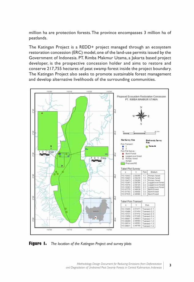
million ha are protection forests. The province encompasses 3 million ha of peatlands.
The Katingan Project is a REDD+ project managed through an ecosystem restoration concession (ERC) model, one of the land-use permits issued by the Government of Indonesia. PT. Rimba Makmur Utama, a Jakarta based project developer, is the prospective concession holder and aims to restore and conserve 217,755 hectares of peat swamp forest inside the project boundary. The Katingan Project also seeks to promote sustainable forest management and develop alternative livelihoods of the surrounding communities.
Figure 1. The location of the Katingan Project and survey plots
4 Introduction
3.2 Basic physical parameters of the study site
3.2.1 Soils
Two formations make up the geological characteristic of the Katingan Project area i.e.,: Alluvial sediment (Co) and Dahor formation (TQd). Most of the soils in the area are considered Organosol glei humus. The soil is characterized as peat, which is naturally acidic at pH levels between 3.0 and 5.0, and is composed of the high accumulation of organic matter substances such as partly decomposed leaves and tree stems. The formation of peat soil in the proposed concession area is a result of constant conditions of water logging above mineral soil and a lack of oxygen, in which a large amount of organic residues are decomposed, forming a peat layer.
3.2.2 Land cover
The Katingan Project area is mostly a peatland, a large part of which is still covered with peat swamp forest. It is characterized by flat terrain with a slope angle of 0-8%, at an altitude of 0-30 meters above sea level. According to a study conducted by the Regional Physical Planning Program for Transmigration1 (RePProt), there are three forest ecosystem proxies within the proposed concession area – peat forest, heath forest and fresh water swamp forest. (see Table 1).
Table 1. Land systems in the Katingan Project area (Source: Landsystem map, RePProt)
ECOSYSTEM Land System RePPProT Size (Ha)
Peat Forest Barah, Gambut, Mendawai 207,921
Fresh Water Swamp Forest Kahayan, Sebangau, Klaru 5,220
Heath Forest Pakau, Segintung 4,614
TOTAL 217,755
Three land cover classes exist in the proposed restoration (i.e., non-forested land, disturbed peat swamp forests and primary peat swamp forests). Small part of non-forest land occurs in the southern part, while disturbed peat-swamp forest extends mostly in the periphery of the proposed restoration.
1] RePProt is a land classification database system developed by the Government of Indonesia for its transmigration program during the 1980s through 1990s. It is the only system, coordinated by the National Land Agency and the Coordinating Agency for Surveys and Mapping, which has been used by all sectors for land-use planning, management and baseline setting until today.

5Methodology Design Document for Reducing Emissions from Deforestation and Degradation of Undrained Peat Swamp Forests in Central Kalimantan, Indonesia
The large part of the primary peat swamp forest stretches from the north to the south in the center of the Katingan Project area.
3.2.3 Rainfall
Average monthly rainfall in the proposed concession is estimated at 240 mm per month with total annual rainfall equal to 2,881 mm per year. Rainfall is relatively evenly distributed throughout the year with all months reportedly receiving more than 200 mm of rain. June through October are generally the driest months, while the wettest months occur in November through May with the average monthly rainfall rises up to 303 mm per month.
3.2.4 Hydrology
The total area of the Katingan Project area is 217,755 ha, which falls between the Mentaya and Katingan Rivers. The flood plains of the two major rivers extend only a short distance from the river banks into forests. Thus, the entire project area receives little nutrient influx from these river floodplains and therefore can be classified as an “ombrogenous” peat swamp. In ombrogenous peat swamps, the only source of nutrient influx is from aerial precipitation (i.e., rain and dust), with small amounts of nutrient influx through microbial nitrogen fixation and faunal migration/animal faeces (Sulistiyanto, 2004).
4. Study Methods
This Methodology Design Document was developed using existing MRV methodologies, reports and literature, as well as field survey results. The below sections describe methods applied to conduct the FS activities and field surveys.
4.1 Carbon MRV methodology
In developing and testing a carbon MRV methodology and monitoring plans, the FS team reviewed and refined existing methodologies, including:
1. Standard operation procedure (SOP) for field measurements2;
2. SOP for allometric equation development and verification3; and
3. Verified Carbon Standard (VCS) methodology for peat swamp forests4.
2] Smith E. M., Gryze S.D., Kusumaatmadja R., Darusman T., and Hardiono M. (2011).3] Sharma B., Gryze S. D., Smith E. M., Silverman J. (2011). 4] Terra Global Capital. (2010).
6 Introduction
The carbon MRV methodology was further tested and developed through field surveys, including:
1. Aboveground forest biomass inventory (aboveground carbon stock measurement) inside 9 nested sampling plots covering 3 forest strata – primary forest5, secondary forest after logging (also denoted as logged-over forest) and secondary forest after forest fires (also fire-damaged/burnt forest);
2. Destructive sampling inside all 9 nested sampling plots to develop a localized allometric equation;
3. Peat survey (belowground carbon stock measurement) at 17 sampling points (9 points inside the nested sampling plots and 8 points along two 1-km line transects);
4. Water level measurement at 17 sampling points using an electric contact meter, and at 2 additional sampling points in logged-over and burnt forest using a HOBO automatic water level recorder6.
Finally, samples and data collected during field surveys were analyzed at a laboratory to estimate aboveground and belowground carbon stocks. Furthermore, to integrate the field survey results into a carbon stock map and stratify forest types, the FS team conducted a remote sensing analysis by using Landsat Thematic Mapper (TM) 5. Survey results and refined SOPs are available in appendices.
4.2 Social safeguards
A social safeguards study was conducted through literature reviews and a field survey in 4 villages in Kotawaringin Timur district located nearby the Katingan Project site.
4.2.1 Data collection
Focus group discussions (FGD) were conducted, using a questionnaire to provide a structure to dialogues. Each FGD accommodated 15-20 participants who are relatively representative of local communities, and provided an opportunity to openly discuss socio-economic conditions, land tenure and livelihoods.
5] No visible sign of logging tracks, canals or stumps 6] HOBO water level data logger with a 100’ range, U20-001-02, available at: http://www.onsetcomp.com/products/kits/
kit-s-u20-02.

7Methodology Design Document for Reducing Emissions from Deforestation and Degradation of Undrained Peat Swamp Forests in Central Kalimantan, Indonesia
4.2.2 Data analysis
Data collected through the FGDs was analyzed in reference to the literature, relevant Indonesian laws and regulations, and previous reports produced under the pre-feasibility study for the fiscal year 2010.
4.2.3 Logical framework
A logical framework was used to review drivers of deforestation and its impacts on peatland forest and local communities’ livelihoods.
4.3 Environmental safeguards
An environmental safeguards study was conducted through a rapid assessment of high conservation value (HCV) species identified in the Katingan Project site.
4.3.1 Field survey
A field survey was conducted in sampling plots along 9 line transects. The sample plots were established based on the local variation of vegetation types within peat swamp ecosystems, levels of disturbance and faunal concentration of rare, threatened and endangered species. At each sample site, the FS team measured and recorded all trees with a diameter at breast height (DBH) greater than 10 cm, identified local species names, and collected leaf samples for a laboratory analysis.
4.3.2 HCV rapid assessment
Based on the high conservation value forest (HCVF) identification toolkit for Indonesia7,Starling Resources’ earlier faunal8 and floral9 reports, and the evaluation of secondary data, the FS team conducted a rapid HCV assessment for the biodiversity components, HCV 1, 2 and 3, to identify the existence of HCV species and prominent threats to them, as well as to produce indicative maps of the area’s forest land systems and HCV species.
5. Outputs
The Methodology Design Document is comprised of three sections – carbon MRV methodology, social safeguards and environmental safeguards,
7] Tropenbos.(2008)8] Harrison et. al (2010)9] Harrison et. al (2011).
8 Introduction
each providing methodologies, approaches and/or recommendations. These were designed as an appropriate means to implementing REDD+ projects in Indonesia under a bilateral corporation mechanism, and carefully reviewed and recommended by the FS team. Furthermore, supplementing documents are provided in the annexes, including:
1. A refined SOP for field measurements;
2. A refined SOP for allometric equation development and verification;
3. Allometric equations for tropical peat swamp forests in the Katingan Project area;
4. Aboveground and belowground carbon stock estimation for the Katingan Project;
5. Environmental safeguard strategies for HCV areas in the Katingan Project area; and
6. Recommendations for next steps after the REDD+ FS 2011.
Additional information, supporting data and references on particular topics (i.e., Carbon MRV, Social safeguards and Environmental safeguards) are separately provided in full reports by the Ministry of Forestry, Republic of Indonesia.
9Methodology Design Document for Reducing Emissions from Deforestation and Degradation of Undrained Peat Swamp Forests in Central Kalimantan, Indonesia
Section I: Carbon MRV Methodology
1.1 Sources
This methodology uses different elements from several approved methodologies and tools. More specifically, this methodology is based on elements from the following methodologies (latest version):
1. Approved CDM Methodology - AR ACM0001 Afforestation and reforestation of degraded land
2. Approved CDM Methodology - AR AM0006 Afforestation/Reforestation with Trees Supported by Shrubs on Degraded Land
This methodology also refers to the latest approved versions of the following tools or modules:
1. VT0001 Tool for the Demonstration and Assessment of Additionality in VCS Agriculture, Forestry and Other Land Use (AFOLU) Project Activities. (Available at http://www.v-c-s.org/tool_VT0001.html)
2. AR AM Tool 03 Calculation of the number of sample plots for measurements within A/R CDM project activities. (Available at https://cdm.unfccc.int/methodologies/ARmethodologies/tools/ar-am-tool-03-v2.pdf
3. Approved VCS Module VMD0014 “Estimation of emissions from fossil fuel combustion (E-FFC)” (Available at http://www.v-c-s.org/methodologies/VMD0014)
Projects that meet the applicability criteria of this methodology will conform to all relevant applicability criteria associated with each of these individual methodologies and tools.
1.2 Summary Description of the Methodology
This methodology sets out the project conditions and carbon accounting procedures for activities aimed at reducing planned deforestation and forest degradation of peat swamp forests, and falls therefore under the “avoided planned peatland deforestation” (APPD) category of the VCS AFOLU requirements. Only one other applicable methodology exists for APPD projects. The proposed methodology differs in some key aspects which may limit the adaptability of the existing avoided planned peat swamp
10 Section I: Carbon MRV Methodology
conversion methodology. More specifically, this methodology offers more flexibility in estimating the baseline deforestation rates, includes a procedure to apply hierarchical forest transition to model the conversion process, uses geostatistical techniques to interpolate peat depths between sampling points, and allows for some small-scale deforestation and forest to be present in the project area. Furthermore, this methodology is developed to be compatible with the new VCS PRC guidelines and uses an internationally accepted definition of peat i.e., containing minimum of 30% organic matters and depth of at least 30 cm (as defined by the Internal Peat Society). The main methodological aspects of the methodology are:
1. The project area must be a production forest i.e. forest land designated for production purposes.
2. Baseline emissions in the project area are calculated based on either legally approved conversion rates or empirically measured historical deforestation rates observed in a reference region similar to the project area.
3. Emissions from non-peat carbon stock densities are quantified by subtracting carbon densities under the project and baseline scenario. Carbon densities for non-peat components are quantified on permanent sampling plots on forest lands or temporary sampling plots on non-forest lands. Emissions from peat carbon stock densities are quantified by measuring or extrapolating the difference in water table and peat subsidence between the project and baseline scenarios. The total net emission reductions are discounted based on the attained precision of biomass, water table, and peat subsidence measurements. If the emissions cannot be measured with sufficient precision, the project is not eligible.
4. Potential emissions from primary leakage are monitored and quantified using a leakage belt approach. Market-effect leakage must be accounted for within each PD, according to the rules set forward within the VCS guidance.
5. While assisted reforestation is not allowed under the VCS AFOLU guidance for REDD projects, natural reforestation and regeneration must be included in the baseline and project scenarios. This is achieved by applying the empirically observed baseline regeneration and reforestation rates in the reference region to the project and baseline scenarios.
6. Assisted natural regeneration activities are allowed as a community development activity, but only to the extent that it increases the baseline natural regeneration rate. The quantification of the GHG benefits from assisted natural regeneration follows a different and more detailed

11Methodology Design Document for Reducing Emissions from Deforestation and Degradation of Undrained Peat Swamp Forests in Central Kalimantan, Indonesia
procedure than for the quantification of GHG benefits from areas without assisted natural regeneration.
7. The methodology is not applicable to grouped projects. However, the project may contain multiple non-contiguous areas. The procedure to account for this is described in section 1.8.1 Describe Spatial Boundaries of the Discrete Project Area Parcels.
1.2.1 Summary of Major Methodological Steps for the Baseline GHG Emissions, Project GHG Emissions, and Monitoring
The PD contains the ex-ante annual net GHG emission reductions due to project activities (NERs) and an estimate of the ex-ante VCUs that are issued after transferring a portion of the NERs to the buffer pool according to the buffer withholding percentage. The actual NERs and VCUs are calculated ex-post based on data collected during monitoring and reported in a monitoring report. The calculation of emission reductions is based on the following principles:
1. This methodology separates emission reductions from avoided deforestation, emission reductions from avoided peat conversion, and carbon uptake through assisted natural regeneration (ANR) because different carbon accounting methods, accuracy thresholds and discounting procedures are applicable on each of these sources:a. The calculation of non-peat related emission reductions from avoiding
deforestation is based on a classification and stratification of the land in discrete classes or forest strata according to the land use and land cover (LULC) or forest type and density. By analyzing transitions from forest classes to non-forest classes, the emissions related to deforestation can be quantified.
b. The calculation of emission reductions from avoided peat conversion is based on (1) measurements of the water table in the project area, and (2) the expected drainage level under project scenario.
c. The accounting for greenhouse gas benefits from assisted natural regeneration (ANR) activities are calculated completely separated using the most recent version of the approved consolidated CDM methodology AR-ACM0001: “Afforestation and Reforestation of Degraded Land”.
2. Significant methane, nitrous oxide and fuel-CO2 emissions from project and community development activities must be subtracted from the NERs.
3. The project must implement activities to minimize any potential emissions from forest degradation from local communities living in or near the

12 Section I: Carbon MRV Methodology
project area. Only significant emissions need to be retained in the final calculations.
1.2.1.1 GHG Sinks and Emissions under the Baseline Scenario
Under this methodology, the most plausible baseline scenario under the CDM modalities and procedures, paragraph 22 is option (c). The calculation of the emissions from deforestation in the project area under the baseline scenario is based on a combination of (1) forest conversion rates from legally recognized documents, or forest conversion rates from a historical remote sensing analysis, (2) biomass inventories to measure the emissions of the non-peat carbon pools after the project area would have been converted, and (3) measurements of the peat depth in the project area and the depth of the water table after conversion to quantify the emissions from the peat carbon pool.
1.2.1.2 GHG Emissions and Sinks under the Project Scenario in the Project Area
For the ex-ante calculations of the project’s GHG emissions, it is assumed that under the project scenario, (1) no conversion takes place inside the project area, but selective logging is allowed under certain applicability criteria, (2) no change in biomass density occurs, apart from areas where sustainable logging is taking place and areas where assisted natural regeneration is performed, and (3) no changes in water table occur. In case the project area is located in Indonesia and the project area is protected by an ecosystem restoration license, logging is not allowed. The carbon accounting for the areas on which assisted natural regeneration activities take place must follow the latest version of approved CDM methodology AR-ACM0001.
1.2.1.3 GHG Emissions under the Project Scenario outside the Project Area (Leakage)
Under this methodology, leakage from shifting of the planned deforestation is calculated by monitoring the planned deforestation activities of the (most likely) deforestation agent in the project area. Leakage from shifting of the extraction of forest products by local communities is calculated by monitoring biomass and deforestation in leakage belts, areas immediately adjacent to the project area.
13Methodology Design Document for Reducing Emissions from Deforestation and Degradation of Undrained Peat Swamp Forests in Central Kalimantan, Indonesia
1.2.1.4 Monitoring Methodology
During the crediting period, all data and parameters that are included in the monitoring tables further in this document must be recorded with the frequency specified. Monitoring has four components: (1) measuring the forest conversion rate within the project area, (2) measuring carbon stock densities per LULC class using field sampling techniques and, (3) measuring the peat depth and the depth of the water table, (4) tracking all GHG emissions from emission sources and (4) monitoring the forest conversion rate outside of the project area by the pre-project deforestation agents.
1.3 Definitions
The definitions below are consistent with or complement the definitions in the VCS AFOLU Requirements. The definitions contained in the Program Definitions document from the VCS shall always have precedence over the definitions introduced in this section.
1.3.1 Definitions Regarding Geographical and Temporal Boundaries
1. The project area is the geographical area where the project participants will implement activities to reduce deforestation. The project area may be contiguous or consist of multiple smaller adjacent and non-adjacent project areas (referred to as discrete project area parcels) and conforms to the definition of “forest” set forward by the VCS Program Definitions.
2. The reference region is the region from which historical land-use change trends are obtained. This information is required to the evolution of future land-use change in the absence of project activities (i.e. baseline scenario). Before the start of the project (i.e. during the historical reference period) the reference region includes the project and leakage areas. After the project has started (i.e. during the crediting period) the reference region excludes the project and leakage areas to serve as a reference for determining deforestation and forest degradation rates in the absence of project activities.
3. The baseline validation period is the period during which the ex-ante calculation of net GHG emissions under the baseline scenario is validated. After the baseline validation period expires, a new ex-ante baseline needs to be calculated and validated by a VCS verifier.

14 Section I: Carbon MRV Methodology
1.3.2 Definitions Regarding Classification and Transition of Land Use and Land Cover
1. In this methodology, units of land are allocated to different land use and land cover (LULC) classes. The LULC classification system must be hierarchical in nature. At the highest level, the definitions from the IPCC GPG-LULCF 2003 for cropland, grassland, settlement, wetland and other land must be followed. A definition of “forest” is included in the VCS Program Definitions.
2. A forest LULC class may be further divided into forest strata according to the carbon stock density, native forest type, past and future management, landscape position, biophysical properties, and the degree of past disturbance. The minimum mapping unit set forward in the forest definition must also be applied to forest strata. The process of sub-dividing the broad forest LULC class into more narrow forest strata is defined as forest stratification.
3. A land transition is a change from one LULC class or forest stratum into another within one geographical area. This methodology considers four main categories of transitions.a. Forest regeneration (RG) is the persistent increase of canopy cover
and/or carbon stocks in an existing forest due to natural succession or human intervention, and falls under the IPCC 2003 Good Practice Guidance land category of forest remaining forest.
b. Increased forest cover is the transition of non-forest land into forest land, and encompasses both reforestation and natural succession.
4. Reforestation (RF) is the human-induced increase in forest cover (e.g., from cropland to forest, or grassland to forest), and is defined in the VCS Program Definitions.
5. Natural succession is a natural increase in forest cover without any human intervention. Natural succession is included in the baseline and project scenarios. Natural succession and increase in forest cover are likely results of decrease in deforestation rate due to project activities.
1.3.3 Other definitions relevant within the scope of this methodology
1. Peat is organic soil with at least 30% organic matter and a minimum thickness of 30 cm.
2. Tropical peat swamp is defined as land containing peat in the tropical or subtropical zone (lying within latitudes 35° North and South). A tropical
15Methodology Design Document for Reducing Emissions from Deforestation and Degradation of Undrained Peat Swamp Forests in Central Kalimantan, Indonesia
peat swamp forest is then defined as land qualifying as forest located on tropical peat swamp.
3. Timber harvesting for local and domestic use. The extraction of timber wood for direct use within the project area and by the households that are living within the project area, without on-sale of the timber
4. Commercial timber harvesting. The extraction of timber wood for further sale on regional/global timber markets outside of the project area or transferred to non-project participants.
5. Participating community. A local community of individuals and households who are permanently living adjacent to the project area, and who are participating in project activities and directly benefit from project activities through increased livelihoods and improved forest resources.
6. Assisted natural regeneration. Any silvicultural activity that accelerates regeneration over natural regeneration rates. Examples of such activities include thinning to stimulate tree growth, removal of invasive species, coppicing, and enrichment planting.
7. A production forest is a forest used for production of various commodities, including timber.
8. A jurisdiction is the legislative territory where power to govern or legislate permits for land and forest concessions is exercised.
1.4 Applicability Conditions
Project proponents must demonstrate that project conditions meet the following list of criteria. Note that in case the project area consists of multiple discrete project parcels, each discrete parcel must meet all applicability criteria of this methodology.
Criteria related to conditions on the land before project implementation:
1. Land in the project area (a) is in the tropical region, (b) qualifies as a forest for at least 10 years before the project start date, and (c) must be a natural forest but may be in a state of partial degradation caused by one or more of the following (legally sanctioned or illegal) drivers of deforestation/degradation:a. Conversion of forest patches to settlementsb. Conversion of forest patches by households for small-scale cropping
(excludes commercial agriculture)c. Small-scale timber logging. Small scale is defined as less than 5% of the
biomass stocks.
16 Section I: Carbon MRV Methodology
d. Collection of fuel-wood or green wood for charcoal productione. Commercial timber harvesting
This methodology takes into consideration that peat swamp forests may be under a dual threat by (1) planned conversion by corporate entities, but also (2) small-scale deforestation from e.g., settlements, conversion for subsistence farming, rubber tapping, and small-scale logging. This methodology provides guidance and procedures to manage such small scale deforestation drivers.
2. The project area is (1) legally designated as forest that can be converted to non-forest or production forest with lower biomass than the original forest by all relevant regional and national authorities, and (2) effectively at threat of conversion as demonstrated by either (2a) sufficient and necessary permit(s) to legally convert the project area by an identified agent of deforestation or (2b) the existence of three conversion permits on other areas within the union of a 250-km buffer around the project area and the jurisdiction with decision-making authority on concession permitting.
3. The baseline rate of conversion of the project area can be quantified as following, separately for each of the conversion strata10, (subsequent options may only be used if prior options are not applicable).a. If the project proponent can produce documentary evidence that
demonstrates a legally approved conversion rate by an identified agent of deforestation, this rate must be used in the carbon accounting for the project. The document used must have all necessary legal approvals and permits.
b. If no such documentary evidence exists, or no specific deforestation agent can be identified, the rate of conversion by the most likely deforestation agent can be determined based on the historical conversion rate by this most-likely deforestation agent in an area similar to the project area (“reference region”). The reference region must consist of at least three areas under the same conversion stratum as the project area within the union of a 250-km buffer around the project area and the jurisdiction with decision-making authority on concession permitting.
c. If option (b) is not applicable, then a conversion rate from the literature may be used for each of the project conversion strata on the condition that it can be demonstrated that this rate (i) is conservative, (ii) is not
10] A conversion stratum is a subset of the project area on which the land sanctioning, conversion threat and the future allowable land-uses are identical.
17Methodology Design Document for Reducing Emissions from Deforestation and Degradation of Undrained Peat Swamp Forests in Central Kalimantan, Indonesia
older than 10 years, (iii) and is from the same country. Section 1.8.2.3 contains further procedures to verify these conditions.
Criteria related to conditions on the land after project implementation:
4. Project proponents shall demonstrate that they have planned conservation activities so that the threat of conversion is reduced. A description of the conservation activities must be presented at every verification.
5. If one or more of the degradation drivers outlined in Applicability Criterion 1 have been active in the past five years in the project area, one or more of the following project activities must be implemented, designed in collaboration with the local communities.a. Supporting alternative livelihood options targeting the communities
active in the forestb. Forest patrolling activitiesc. Fire controlsd. Supporting the use of fuel-efficient stovese. Establishment of sustainable fuel-wood lotsf. Agricultural intensification.
6. Development of new drainage or continuation/maintenance of active drainage canals within the project boundary is not eligible.
7. If the area that is hydrologically connected to the project area in which peat is present extends beyond the project area boundary, it is required to establish a buffer zone around the project area with peat. It must be ensured that no draining occurs in this buffer zone. It is allowed that the buffer zone extends beyond the project area boundary if legally binding agreements are put in place with land owners of the land outside the project area to ensure that no draining occurs in the buffer zone. However, if such agreements cannot be established, the buffer zone must be established inside the project boundary. In the event that land owners in the buffer zone violate the agreement and begin drainage activities in the buffer zone, the buffer zone shall be immediately redrawn inside the project boundary and credits shall be calculated using the updated buffer zone from the moment the violation occurs and impacts emissions in the project area. The width of the buffer zone must be established using the procedures in Section 1.8.1.
8. No clear-cut or patch-cut harvesting of timber is allowed in the project areas. However, selective harvesting of timber is allowed on the following conditions.
18 Section I: Carbon MRV Methodology
a. The emissions related to the loss of biomass during harvesting (“harvest emissions”) are duly accounted for and subtracted from the emission reductions.
b. For every verification period, the harvest emissions are smaller than the net emission reductions without harvesting generated during that verification period, so that no “negative credits” are generated.
c. Selective harvesting shall not significantly affect the hydrology of the peat layer and cause peat decomposition. Harvest activities do not require the development or maintenance of drainage canals in the project area
d. In case the project area is located in Indonesia, the project area shall not be protected by an ecosystem restoration license.
9. The magnitude of activity-shifting leakage by communities present within the project area or using the project area is quantified through a rigorous monitoring plan consisting of rural appraisals, remote sensing analysis and biomass inventories in the project area and all leakage belts11. The exact procedures for doing so are included in this methodology.
Other criteria:
10. Subsequent to the removal or disappearance of carbon in the above ground live biomass pool, carbon in the below ground biomass pool is also removed or disappears within the duration of the project. The removal of the belowground biomass can be caused by anthropogenic activities such as digging, extraction of stump, and burning, or by the natural process of decay and decomposition12.
11. The maximum quantity of GHG emission reduction claimed by the implemented project from peat component shall not exceed the net GHG benefits generated by the project 100 years after the start date. This condition must be verified using the procedures in Section 1.11.4.
1.5 Project Boundary
1.5.1 Gases
This methodology requires accounting of emissions of all three biogenic greenhouse gases (CO2, N2O and CH4) from sources not related to changes
11] Geographically constrained drivers may induce leakage in the leakage belt, which is the area in the immediate vicinity of project areas. The methodology contains procedures to determine the location of the leakage belt.
12] This must be justified using appropriate literature sources such as Chambers et al. (2000).

19Methodology Design Document for Reducing Emissions from Deforestation and Degradation of Undrained Peat Swamp Forests in Central Kalimantan, Indonesia
in carbon pools, henceforward referred to as “emission sources” (Table C1)13. Project proponents may omit certain emission sources, but only if they can prove that their contributions are insignificant. The VCS defines significant sources as those accounting for more than 5% of the total GHG benefits generated.
Table 2. GHG emissions from sources not related to changes in carbon pools (“emission sources”) to be included in the GHG assessment.
Potential Emis-sion Source Gas In-
clude? Justification/Explanation
Base
line
Removal of live biomass
CO2 No Emissions are related to changes in carbon pools
CH4 No Negligible
N2O No N2O emissions from fire are conservatively ex-cluded.
Burning of peat
CO2 Yes Emissions are related to changes in carbon pools
CH4 Yes Major source of emissions under the baseline scenario
N2O No Major source of emissions under the baseline scenario
Peat oxida-tion from drainage
CO2 Yes Major source of emissions under the baseline scenario
CH4 No Negligible
N2O No Negligible
Proj
ect
Increased area of rice production systems
CO2 No Not applicable
CH4 Yes Potentially major source
N2O No Not applicable
Increased fertil-izer use for agricultural intensifica-tion
CO2 No Not applicable
CH4 No Not applicable
N2O Yes Potentially major source
Removal of biomass to prepare assisted natural re-generation
CO2 Yes Potentially major source
CH4 Yes Potentially major sourceif controlled burning is used
N2O No N2O emissions from burning are insignificant
13] Nitrous oxide emissions from forest fires (excluding controlled burning as a silvicultural activity) are excluded from the GHG accounting.
20 Section I: Carbon MRV Methodology
1.5.2 Carbon Pools
Table 2 summarizes the carbon pools that must be included in projects following this methodology.
Table 3. Selected Carbon Pools
Carbon Pool Included? Justification/ Explanation of ChoiceAbove-ground tree biomass
Included Major carbon pool affected by project activities
Above-ground non-tree biomass
Included Change expected to be positive or insignificant under the applicability criteria.
Below-ground biomass Included Major carbon pool affected by project activities
Dead wood Included Major carbon pool affected by project activities
Litter Included Potentially significant carbon pool.
Soil organic carbon (including peat)
Included Major carbon pool affected by project activities
Long-lived Wood products
Included Logging may have been present under baseline conditions. Therefore, halting logging may decrease carbon stored in long-lived wood products.
1.5.3 Spatial and Temporal Boundaries
The spatial boundaries of the project area must be unambiguously defined in the PD. The project area may be contiguous or consist of multiple adjacent or non-adjacent parcels, “discrete project area parcels”. Around each discrete project area parcel, a leakage belt shall be defined. Before the start of the project, the reference region must include the project area and leakage area. After the start of the project, the reference region may not contain the project area and leakage belt.
A map indicating the extent of the area that is hydrologically connected to the project area in which peat is present shall be presented at validation. This map must contain the extent of the buffer zone as specified in applicability condition 7. The area that is hydrologically connected to the project area shall be determined using a hydrological model using bulk density and peat depth data measured at project site to simulate the water table depth under known hydrological conditions according to the following flow diagram.
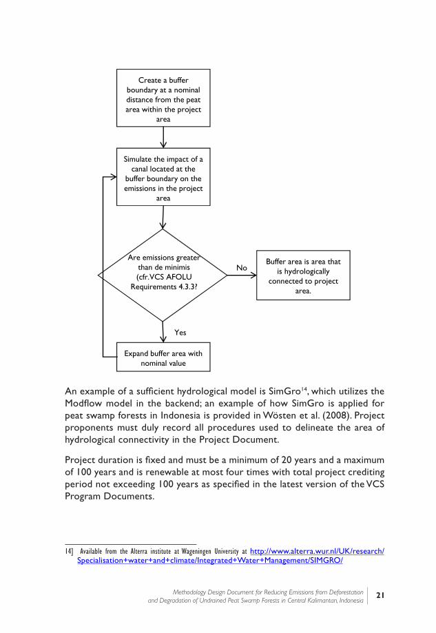
21Methodology Design Document for Reducing Emissions from Deforestation and Degradation of Undrained Peat Swamp Forests in Central Kalimantan, Indonesia
Create a buffer boundary at a nominal distance from the peat area within the project
area
Simulate the impact of a canal located at the
buffer boundary on the emissions in the project
area
Are emissions greater than de minimis (cfr.VCS AFOLU
Requirements 4.3.3?
Buffer area is area that is hydrologically
connected to project area.
Yes
No
Expand buffer area with nominal value
An example of a sufficient hydrological model is SimGro14, which utilizes the Modflow model in the backend; an example of how SimGro is applied for peat swamp forests in Indonesia is provided in Wösten et al. (2008). Project proponents must duly record all procedures used to delineate the area of hydrological connectivity in the Project Document.
Project duration is fixed and must be a minimum of 20 years and a maximum of 100 years and is renewable at most four times with total project crediting period not exceeding 100 years as specified in the latest version of the VCS Program Documents.
14] Available from the Alterra institute at Wageningen University at http://www.alterra.wur.nl/UK/research/Specialisation+water+and+climate/Integrated+Water+Management/SIMGRO/

22 Section I: Carbon MRV Methodology
Reporting requirements in the PD1. Evidence that each of the applicability conditions is met.
2. The project location description as required by the VCS Program Documents.
3. A list of specific sources of greenhouse gases that will be considered in the project based on Table 1.
1.6 Procedure for Determining the Baseline Scenario
The most current version of the VCS “VT0001 Tool for the Demonstration and Assessment of Additionality in VCS Agriculture, Forestry and Other Land Use (AFOLU) Project Activities” must be used to determine the most likely baseline scenario.
1.7 Procedure for Demonstrating Additionality
The most current version of the VCS “VT0001 Tool for the Demonstration and Assessment of Additionality in VCS Agriculture, Forestry and Other Land Use (AFOLU) Project Activities” must be used to determine additionality.
PD Reporting requirements 1. Demonstration on how the project is additional using the additionality
tools from the VCS.
The most current version of the VCS “VT0001 Tool for the Demonstration and Assessment of Additionality in VCS Agriculture, Forestry and Other Land Use (AFOLU) Project Activities” must be used to determine the most likely baseline scenario. The procedures described in VCS tool VT0001 must be followed to identify and analyze the alternative baselines. The most plausible baseline must be selected from the list of available alternative baselines using the step-wise approach below. The selected baseline shall be planned conversion to a non-forest land use. The areas or strata where the most plausible baseline scenario is not the planned conversion of forest to non-forest land-use shall be excluded from the project area. The following steps must be repeated for each of the strata of the project area to justify the selected baseline scenario:
1. Demonstrate that the project area is suitable for selected alternative non-forest land-use. Suitability of conversion to non-forest land-use
23Methodology Design Document for Reducing Emissions from Deforestation and Degradation of Undrained Peat Swamp Forests in Central Kalimantan, Indonesia
must be described by providing a detailed account of accessibility to relevant markets for the goods and services derived from project area, and suitability of soils, topography and climate for intended conversion. Exclude any areas that were found to be unsuitable for non-forest land-uses from the project.
2. For all the areas that were found to be suitable for conversion to non-forest land-use, enumerate and describe all the possible agents of planned forest deforestation in the region. An agent of the planned deforestation can be either the land-owner, or the right holder.a. If a specific agent of deforestation can be identified, it must be
demonstrated that this specific agents of planned deforestation is likely to proceed with conversion within the project credit period in absence of AFOLU project. The likelihood of deforestation by the specific agent of deforestation must be demonstrated by providing documentary evidence that demonstrates legally approved conversion by the identified agent of deforestation. The evidence used may be one or more of the following:• Valid forest conversion license owned by agent of deforestation.
• Documentation that a request for approval for forest conversion has been filed with the tenure holder and relevant government department, if applicable.
• Documentation that provides evidence of landowner investment to establish suitability of project lands to proposed post-deforestation land use.
• Record of planned deforestation activities of agents in the past 10 years in the country.
• Purchase offer of the project area by an entity to convert the land to non-forest land-use
• Bid for conversion announced by the land-owner. b. If no specific agent of deforestation can be identified, the likelihood of
deforestation must be demonstrated through the existence of three conversion permits on other areas within the union of a 250-km buffer around the project area and the jurisdiction with decision-making authority on concession permitting.
3. The justification of selection of a baseline scenario is strong when more than one of the criteria mentioned above holds true or when more than three conversion permits are presented. When multiple deforestation agents are identified, the most plausible agents for that spatial unit must be selected.
24 Section I: Carbon MRV Methodology
4. Provide a description of the planned conversion activities of the most plausible agent of planned deforestation in areas similar to the project area. If the most likely agent can be specifically identified but has never converted areas similar to project area, then project proponents must demonstrate that it is indeed likely that such conversion may take place in absence of the project activity. The propensity of conversion can be demonstrated by providing a verifiable description of conversions taking place within the jurisdictions such as province, state or region within the past 10 years. The descriptions could be augmented with relevant documents, images and maps, if available. Verifiable historic account of such conversion may come from several sources including scientific publications based on primary data using social assessment, government records, remote sensing assessments and management plans.
1.8 Quantification of GHG Emission Reductions and RemovalsBaseline Emissions
1.8.1 Select Spatial and Temporal Boundaries
This step includes the demarcation the project area and the reference region.
1.8.1.1 Describe Spatial Boundaries of the Discrete Project Area Parcels
Project proponents shall provide digital (vector-based) files of the discrete project area parcels Keyhole Markup Language (KML) file format as required by VCS. A clear description must accompany each file, and the metadata must contain all necessary projection reference data. In addition, the PD must include a table containing the name of each discrete project area parcel, the centroidcoordinate (latitude and longitude using a WGS1984 datum), thetotal landarea in ha, details of tenure/ ownership/zoning and the relevant administrative unit belongs to (county, province, municipality, prefecture, etc.).
1.8.1.2 Stratify Each Unique Project Parcel According to Potential Conversion Scenario
Stratify each unique project parcel according to the most likely land conversion that will take place on the land. For each of the legal zoning categories present on the land, identify the most likely conversions based on (a) previous official applications of concessions in the project area, or (b) previous active concessions in the project area that are not active anymore, or (c) common
25Methodology Design Document for Reducing Emissions from Deforestation and Degradation of Undrained Peat Swamp Forests in Central Kalimantan, Indonesia
practice.Identify the most relevant conversion scenarios that may be present on the land while taking into account any legal limits and requirements for the conversion.
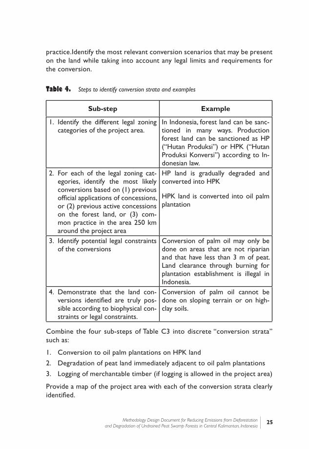
Table 4. Steps to identify conversion strata and examples
Sub-step Example
1. Identify the different legal zoning categories of the project area.
In Indonesia, forest land can be sanc-tioned in many ways. Production forest land can be sanctioned as HP (“Hutan Produksi”) or HPK (“Hutan Produksi Konversi”) according to In-donesian law.
2. For each of the legal zoning cat-egories, identify the most likely conversions based on (1) previous official applications of concessions, or (2) previous active concessions on the forest land, or (3) com-mon practice in the area 250 km around the project area
HP land is gradually degraded and converted into HPK
HPK land is converted into oil palm plantation
3. Identify potential legal constraints of the conversions
Conversion of palm oil may only be done on areas that are not riparian and that have less than 3 m of peat. Land clearance through burning for plantation establishment is illegal in Indonesia.
4. Demonstrate that the land con-versions identified are truly pos-sible according to biophysical con-straints or legal constraints.
Conversion of palm oil cannot be done on sloping terrain or on high-clay soils.
Combine the four sub-steps of Table C3 into discrete “conversion strata” such as:
1. Conversion to oil palm plantations on HPK land
2. Degradation of peat land immediately adjacent to oil palm plantations
3. Logging of merchantable timber (if logging is allowed in the project area)
Provide a map of the project area with each of the conversion strata clearly identified.

26 Section I: Carbon MRV Methodology
1.8.1.3 Specify Temporal Boundaries of the Project
Project proponents must fix the following temporal boundaries:
1. The historical reference period with exact start date. The end of the historical reference period must coincide with the project start date. The duration of the historical reference period must be between 6 and 10 years.
2. The project crediting period with exact start date and project end date. The start of the crediting period is equal to the start of project date and is the date when the first project activity for which NERs are claimed is implemented. The duration of the crediting period must be between 20 and 100 years.
3. Project proponents must seek third-party verification at least every five years. The frequency of verification may change during the crediting period (e.g., every two years during the first ten years of the crediting period, and every five years thereafter). The frequency and years of verification must be fixed for the duration the baseline is valid and must be included in the PD or in a monitoring report if the baseline is updated.
Baselines must be updated at year five, ten and every ten years thereafter. Under specific circumstances, the baseline must be updated more frequently. These circumstances are outlined in the monitoring section.
Reporting Requirements in the PD1. Maps for all project areas with the LULC classes and forest stratification.2. Shape files of the discrete project area parcels and the reference region1.
All necessary meta-data to correctly display the files must be included.3. Table of all the discrete project area parcels with their ID, name, coordi-
nate centroid (latitude and longitude using a WGS1984 datum), total land area in ha, details of tenure/ownership, and the relevant administrative unit.
4. Overview map of the whole reference region with the location of the discrete project area parcels clearly indicated.
1.8.2 Determine Baseline Conversion Rates
As specified in the applicability criteria, three options exist to determine the baseline rate of conversion of the project area. The conversion rate must be estimated separately for each of the project conversion strata. Note that subsequent options may only be used if prior options are invalid or not
27Methodology Design Document for Reducing Emissions from Deforestation and Degradation of Undrained Peat Swamp Forests in Central Kalimantan, Indonesia
applicable. Different conversion strata within one project may use different options to determine the baseline conversion rate.
1.8.2.1 Option (a) - Legally Approved Conversion Rate
If the project proponent can produce documentary evidence that demonstrates a legally approved conversion rate for the project area by an identified agent of deforestation, this rate must be used in the carbon accounting for the project. Examples of such evidence include legally approved management plans, management maps, etc. The documents provided as evidence used must have all necessary legal approvals and permits. However, the permits may not be valid any longer due to the existence of the REDD project.
1.8.2.2 Option (b) – Historical Conversion Analysis in a Reference Region
In case no legally recognized forest conversion rate is available, the rate of deforestation and forest degradation in the project area under the baseline scenario may be calculated from the reference region which is used as a proxy for the baseline calculations within the project area. The reference region consists of at least three areas that have a similar land conversion stratum as the ones identified in the project area, but on which the conversion has already occurred in the reference region that includes a 250-km buffer around the project boundary and the jurisdictional area. The quantification of the conversion rate shall only be based on the land that is legally allowed to be converted using current legal restrictions, even if such restrictions were not into force at the time the historical conversion occurred. Land that has been converted but is not allowed to be convert according to current legal restrictions shall be excluded from the conversion rate calculation.
To determine the conversion rate on the three areas, at least two maps of forest cover are required: at least one image from 0-5 years before project start, and (b) at least one image from 5-15 years before project start. There must be at least 5 years difference between the two maps of forest cover. If no forest cover maps are available, a remote sensing-based forest cover map must be developed. The spatial resolution of the remote sensing data used to create these maps must be at least 30m. The LULC classes used during classification must contain at least the six IPCC LULC classes (Forest Land, Crop Land, Grass Land, Wetlands, Settlements, and Other Land) in the LULC class definitions. The definition of these classes must be consistent with Chapter 2 of the IPCC GPG-LULUCF 2003. In cases where the country has defined more specific LULC classes than the IPCC classes, these definitions

28 Section I: Carbon MRV Methodology
must be used if they are accurate enough for project-specific classification. All steps involved in pre-processing (e.g., orthorectification, cloud masking, haze removal, radiometric corrections), classification (e.g., (sub-)pixel based or segment-based), and post-processing (e.g., spatial and temporal filtering) must be duly noted in the PD. In addition, an independent accuracy analysis must be included. The accuracy assessment of the LULC classification and forest stratification process must follow the best practices for remote sensing (e.g., Congalton 1991). The LULC classes or forest strata for these reference locations must be identified using field observations, in-situ maps, remote sensing data, and other ground-truthing data. At least 50 reference locations per LULC class or forest stratum must be used. More specifically, the classification accuracy must be assessed by comparing the classes of the points from the validation dataset with the classes of the same locations on the classification products. A confusion matrix or error matrix will be produced together with different statistical measures of overall accuracy, producer’s accuracy, user’s accuracy and kappa statistics for each classified image. Similarly, classification within the classes must be conducted to account for degradation i.e. multiple classless within the strata within a land cover classes for each classified image. Every individual image shall meet the accuracy threshold of 70%. In addition, the smallest accuracy across all images shall be used for discounting purposes as described in Table 5.
Table 5. Accuracy discounting factors for LULC classification as a function of the small-est attained accuracy across all images used.
Discounting factor for emission reductions from avoided deforestation based on the accuracy of LULC classification
Smallest accuracy attained>85% 1.0080-85% 0.8575-80% 0.8070-75% 0.75<70% Project is not eligible
The historical conversion rate, (i.e., proportion of converted forest area divided by the total forest area of the earliest LULC map) must be interpolated for each of the conversion strata in the project area by multiplying the rate with the area of the conversion stratum. Present a table of annual deforested area,
29Methodology Design Document for Reducing Emissions from Deforestation and Degradation of Undrained Peat Swamp Forests in Central Kalimantan, Indonesia
as well as the remaining forest cover for each conversion stratum. Obviously, conversion must stop after no more forest is available so that the remaining forest cover remains positive.
1.8.2.3 Option (c) – Conservative Estimate of a Conversion Rate
If option (a) or option (b) are not applicable, a conversion rate obtained from the literature may be used on the condition that it can be demonstrated that (i) it is conservative, (ii) it is not older than 10 years and (iii) it is from the same country or province as the project area. It is up to the project proponent to demonstrate that the selected rate is valid and conservative. The validator will assess the conservativeness of the selected rate on the following basis:
1. Applicable rates must be acquired from literature sources such as peer-reviewed literature, official land use change maps and reports. Project proponents must substantiate why a proposed rate is applicable. At least three different rates from three different and independent sources from within the past 10 years must be presented in the PD so that the auditor can assess the conservative nature of the selected values
2. The most conservative rate (i.e., smallest of the available rates) must be used. The Project Design Documents must state available rates and the justification for the used value as most conservative.
3. The rates used or proposed by project proponents must be cross-checked for conservativeness in scientific publication archives by the validator. Common scientific archives are ISI Web of Knowledge, Google Scholars, Agricola, PubMed or similar archives that index scientific publications.
However, even if all of the conditions above are met, an auditor has the authority to disapprove validation of a project when doubt remains on the conservative nature of the proposed conversion rate.
The existing peat conversion methodology uses a conversion rate based on legal permits, management plans, or other valid documentation, which is, oftentimes, difficult to access. Even though deforestation is evident from remote sensing data, no documentation may exist to substantiate the deforestation rate. This methodology includes the option to infer the baseline deforestation rate from remote sensing analyses combined with records of land sanctioning, which are usually available. The methodology includes three different approaches to quantify the baseline emissions rate in peat forests. Such flexibility is particularly relevant in countries where management plans do not always contain information on conversion rates.
30 Section I: Carbon MRV Methodology
Reporting Requirements, include in the PD sections 2.3 and 2.41. For option (a): list of the documentary evidence used for the legally
approved conversion rate (option a).
2. For option (b): description of the maps used for the historical analysis or remote sensing data used, detailed description of the remote sensing procedures, and a report on the accuracy of the remote sensing analysis.
3. For option (c): justification of the used source including rationale on conservative nature and validity of the source.
4. Table of annual deforested area, as well as the remaining forest cover for each conversion stratum.
1.8.3 Determine Plant Emission Factors for All Included Transitions
For each LULC class or forest stratum that could be subject to a transition as identified in section 1.8.3.1, it is necessary to determine the average carbon stock density, based on permanent sampling plots on forest LULC classes (including fully stocked and degraded forest areas) and non-permanent sampling plots on non-forest LULC classes (including degraded woodlands, oil palm plantations, and agriculture). The number of plots and their location must be determined in a stratified sampling design. The following steps are to be followed:
1. Identify the LULC classes and forest strata for which carbon stocks are to be quantified.
2. Review existing biomass and biomass increment data for comparison with field measurements.
3. Determine the sample size per LULC class or forest stratum.
4. Measure carbon density stocks of each LULC class or forest stratum.
5. Calculate emission factors for each land transition category.
1.8.3.1 Identify the LULC Classes and Forest Strata for which Carbon Stocks are to be Quantified.
Present a table of all transitions between LULC classes and forest strata that are likely to occur for every conversion stratum in a table similar to Table 5. The main categories of transitions are deforestation, forest degradation, increased forest cover and regeneration. A list must be prepared of the transitions that are considered by the project proponents by analyzing a matrix
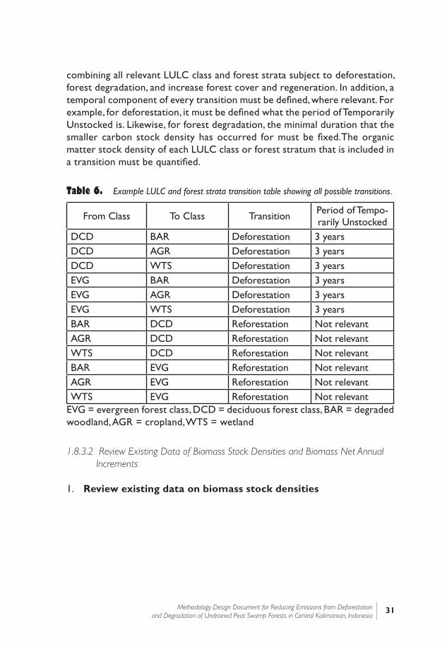
31Methodology Design Document for Reducing Emissions from Deforestation and Degradation of Undrained Peat Swamp Forests in Central Kalimantan, Indonesia
combining all relevant LULC class and forest strata subject to deforestation, forest degradation, and increase forest cover and regeneration. In addition, a temporal component of every transition must be defined, where relevant. For example, for deforestation, it must be defined what the period of Temporarily Unstocked is. Likewise, for forest degradation, the minimal duration that the smaller carbon stock density has occurred for must be fixed.The organic matter stock density of each LULC class or forest stratum that is included in a transition must be quantified.
Table 6. Example LULC and forest strata transition table showing all possible transitions.
From Class To Class Transition Period of Tempo-rarily Unstocked
DCD BAR Deforestation 3 yearsDCD AGR Deforestation 3 yearsDCD WTS Deforestation 3 yearsEVG BAR Deforestation 3 yearsEVG AGR Deforestation 3 yearsEVG WTS Deforestation 3 yearsBAR DCD Reforestation Not relevantAGR DCD Reforestation Not relevantWTS DCD Reforestation Not relevantBAR EVG Reforestation Not relevantAGR EVG Reforestation Not relevantWTS EVG Reforestation Not relevant
EVG = evergreen forest class, DCD = deciduous forest class, BAR = degraded woodland, AGR = cropland, WTS = wetland
1.8.3.2 Review Existing Data of Biomass Stock Densities and Biomass Net Annual Increments
1. Review existing data on biomass stock densities

32 Section I: Carbon MRV Methodology
For the purpose of sampling design and quality assurance of the measured values, all existing data on biomass stock densities must be reviewed. Sources that must be consulted include (lower-ranking options may only be used if higher-ranking options are not available): (a) peer-reviewed scientific literature conducted within the reference region, (b) peer-reviewed scientific literature from an area similar to the reference region, (c) non peer-reviewed reports or studies from the reference region or similar areas. Sources that contain a measure of the variation of the values (range, standard deviations, standard errors, or coefficients of variation) are specifically useful, since these can be used for preliminary determination of the number of sampling plots required during field sampling. For every data source used, note the following items:
1. Methodology (field inventory, extrapolation from satellite imagery, ecosystem model, or GIS analysis).
2. Number of measurement plots used.
3. Whether all species are included in the sampling.
4. The minimum DBH of measured trees in the biomass inventory.
5. Region in which the samples were taken.
2. Review existing data on net annual increments of biomass
Whereas the GHG benefits from avoided deforestation and avoided forest degradation are based on observed transitions between LULC classes and forest strata, the GHG benefits from ANR activities are based directly on the empirically observed increases in biomass stock densities. Therefore, a correct accounting of the GHG benefits from ANR activities requires a sound baseline natural regeneration rate. Therefore, for accurate ex-ante estimates, all existing data on net annual increments of biomass carbon stocks must be reviewed. Sources that must be consulted include (lower-ranking options may only be used if higher-ranking options are not available): (1) values measured by the project proponents in the project area using the methods used for forest inventories discussed in this methodology, (2) national or local growth curves and tables that are usually used in national or local forest inventories, (3) values from peer-reviewed literature, report the items above, (4) values from GPG-LULUCF Table 3A.1.5. These values are representative for regeneration in well-managed forests, and will therefore be conservative. These values must be reported as for every stratum on which ANR activities are planned. For any values used other than the ones given in GPG-LULUCF Table 3A.1.5, the estimated values must be proportionally discounted if the uncertainty (percentage of mean) exceeds 15%.
33Methodology Design Document for Reducing Emissions from Deforestation and Degradation of Undrained Peat Swamp Forests in Central Kalimantan, Indonesia
1.8.3.3 Determine the Sampling Design, i.e., Number, Location, and Layout of Biomass Plots
This section relates to determining the sampling design for biomass plots. The sampling design for peat depth locations is explained in Section 1.8.4.2. The sampling of peat may follow a different sampling design than the sampling of aboveground biomass.
The determination of the sample size (number of biomass sampling plots) required per LULC class and forest strata that are identified in 8.1.3.1 is dependent on (1) the required precision of 15% at 95% confidence level and (2) the variance in the specific LULC class and forest strata. A similar sampling design is used to determine the peat depth and water table measurement and wherever applicable, measurements occur together on the same plots. Extra measurement plots must be installed within the ANR areas to reliably estimate the increase in carbon density. Use AR-AM Tool 03 (“Calculation of the number of sample plots for measurements within A/R CDM project activities”) to determine the number of biomass inventories required.
Further explanation on how to select the layout of biomass sampling plots (form, nesting, etc.) can be found in textbooks such as Hoover (2008). For measuring and monitoring carbon density in the forest strata, a network of permanent forest sampling plots must be established. Due to the significant anthropogenic influence on non-forest land, it is not deemed feasible to install permanent sampling plots. Therefore, the average carbon stock density on non-forest LULC classes shall be assessed using non-permanent sampling plots. Alternatively, conservative defaults gathered from scientific literature may be used to quantify the carbon stock density on non-forest land. The applicability of these default values shall be confirmed by the validator.
Within a LULC class or forest stratum, the location of biomass sampling plots must be selected either systematically with a random start (see 2003 IPCC GPG-LULUCF) randomly within a cell of a systematic grid (see Thompson, 2002), or using a systematic grid. The randomization must be done ex-ante by a computer program. This is required to avoid subjective choice of plot locations. For each sample plot, record the observed LULC class, forest type, and estimated forest canopy closure.
Summarize the sampling framework following the guidance of section 4.3.3.4 of GPG LULUCF in the PD and provide a map and the coordinates of all sampling locations.

34 Section I: Carbon MRV Methodology
1.8.3.4 Measure Plant Carbon Stock Density
The aboveground plant carbon stock density from a sampling plot is calculated by summing the aboveground and dead-wood components of this plot. The belowground plant carbon stock density shall be kept separate from the aboveground plant carbon stock density.
1.8.3.5 Measure Plant Carbon Stock Density
The aboveground plant carbon stock density from a sampling plot is calculated by summing the aboveground and dead-wood components of this plot. The belowground plant carbon stock density shall be kept separate from the aboveground plant carbon stock density.
[EQ1]
Where:
= Total aboveground plant organic matter density of plot within LULC class or forest stratum . [Mg DM ha-1]
= Belowground tree organic matter of plot within LULC class or forest stratum . [Mg DM ha-1]
= Lying deadwood organic matter of plot within LULC class or forest stratum . [Mg DM ha-1]
= Standing deadwood organic matter of plot within LULC class or forest stratum . [Mg
DM ha-1]
= Aboveground tree organic matter of plot within LULC class or forest stratum .[Mg
DM ha-1]

35Methodology Design Document for Reducing Emissions from Deforestation and Degradation of Undrained Peat Swamp Forests in Central Kalimantan, Indonesia
For either the aboveground or belowground plant organic matter densities, the average stock densities of stratum and associated statistics are calculated on the plots within LULC class orforeststratum .
[EQ2]
[EQ3]
[EQ4]
[EQ5]
= Average plant organic matter density of LULC class or forest stratum . [Mg DM ha-1]
= Total biomass stock density of plot within LULC class or forest stratum . [Mg DM ha-1]
= Standard deviation of the total plant-derived organic matter density of LULC class or forest stratum . [Mg DM ha-1]
= Standard error of the average of the total plant-derived organic matter density of LULC class or forest stratum . [Mg DM ha-1]
= Number of sampling plots ofLULC class or forest stratum . [-]
= Half-width of the confidence interval around the average of the total plant-derived organic matter density of LULC class or forest stratum . [Mg DM ha-1]
= Value of t-statistics (i.e., from t-table) at 95% confidence interval and n-1 degree of freedom [-]
The average total carbon stock is calculated by multiplication with the carbon fraction:

36 Section I: Carbon MRV Methodology
[EQ6][EQ7]
Where:
= Average aboveground plant carbon stock density of LULC class or forest stratum . [MT C ha-1]
= Carbon fraction of dry matter in wood (default = 0.5). [Mg C (Mg DM)-1]
= Total aboveground plant-derived organic matter of LULC class or forest stratum . [Mg DM ha-1]
= Average belowground plant carbon stock density of LULC class or forest stratum . [MT C ha-1]
= Total belowground plant-derived organic matter of LULC class or forest stratum . [Mg DM ha-1]
The exact measurement of above-ground and below-ground tree carbon must follow international standards and follow IPCC GPG LULUCF 2003. These measurements are explained in detail in CDM approved methodology AR-AM0002 “Restoration of degraded lands through afforestation/reforestation”. A step-by-step Standard Operations Procedure for field measurements must be prepared ex-ante and contain a detailed, step-by-step explanation of all of the required field-work for both ex-ante and ex-post measurements. This document will ensure consistency during the crediting period by standardizing sampling procedures from year to year.
1. Aboveground tree biomass, . The aboveground tree biomass must be calculating by measuring the DBH of all trees with a DBH > 5 cm within the sampling plot. The applicability of the allometric equation used must be specifically verified according to the procedures of this methodology described in Section 10.4. The allometric equation(s) must remain fixed during a baseline validation period. During verification, project proponents may propose to replace previously used allometric equations, and BEF values by more accurate ones, if these would become available. The use of different allometric equations and BEF values is subject to the explicit approval of the validator.
2. Aboveground non tree biomass, . The above ground non-tree vegetation must be measured by destructive harvesting techniques. If litter is included in the biomass inventories, litter shall be added to the aboveground non tree biomass pool.

37Methodology Design Document for Reducing Emissions from Deforestation and Degradation of Undrained Peat Swamp Forests in Central Kalimantan, Indonesia
3. Belowground biomass, . The below-ground biomass pool must be estimated from the above-ground biomass using
a relationship between aboveground and belowground biomass, such as a root-to-shoot ratio. The assumptions for using a root-to-shoot ratio are verified in the applicability criteria.
Similar as to the constants for the aboveground biomass,
must befixed during a baseline validation period. During baseline validation, project proponents may replace a previously used
by a more accurate one, if this would become available.
4. Lying dead-wood, . Lying deadwood must be sampled with the line intersect method (Harmon and Sexton, 1996) using the equation by Warren and Olsen(1964) as modified by Van Wagener (1968).
5. Standing dead-wood, . Standing dead trees shall be measured using the same procedures used for measuring live trees with the addition of a decomposition class.
1.8.3.6 Calculate Emission Factors and Temporal Component of Belowground Biomass
Emission factors only include the carbon pool-related sources due to changes in biomass between the LULC classes and forest strata. Since N2O and CH4 emissions from forest fires increase emissions, they can be conservatively omitted for baseline calculations15. Once the carbon stock densities are calculated, biomass carbon emission factors and their uncertainties for each LULC class or forest stratum transition are calculated as:
[EQ8]
[EQ9]
15] Note that under the project scenario, N2O emissions from controlled burning must be included in the carbon accounting.

38 Section I: Carbon MRV Methodology
= Emission factor for change in aboveground plant organic matter from LULC class or forest stratum 1 to 2. [tCO2e ha-1]
= Land transition from LULC class or forest stratum 1 to 2.
= Carbon density of aboveground plant organic matter of classes or forest stratum . [MT C ha-1]
= Total emission factor for change in belowground plant organic matter from LULC class or forest stratum 1 to 2. [tCO2e ha-1]
= Carbon density of belowground plant organic matter of classes or forest stratum . [MT C ha-1]
For either the aboveground or total belowground emission factor, the combined error in estimated biomass stock densities for a transition from one stratum to another is measured as:
[EQ10]
If the combined error is smaller is than 0.15, no deduction is applied and the discounting factor for uncertainty around biomass stock densities is set to 1 as:
[EQ11]
If the combined error is greater than 1, the discounting factor for uncertainty around biomass stock densities is set to 0 as:
[EQ12]

39Methodology Design Document for Reducing Emissions from Deforestation and Degradation of Undrained Peat Swamp Forests in Central Kalimantan, Indonesia
However, if the combined error is greater than 0.15 and smaller than 1, then the discounting factor for uncertainty around biomass stock densities is obtained as:
[EQ13]
Where:
= Discounting factor for the emission factor for the transition from LULC class or forest stratum 1 to class 2 according to the uncertainty of the biomass inventory. [-]
and
= Half-width of the 95% confidence interval around the mean plant organic matter density of LULC classes or forest strata 1 and 2. [tCO2e ha-1]
= Combined error in estimated biomass stock density change for a transition from one stratum to another. [-]
Note that a positive sign of indicates a net sequestration of carbon, or an increase in the carbon stock, and a negative sign indications emission. List the estimated emission factors, the associated uncertainties, and the lower confidence limit per LULC class and forest strata category in a table in the PD. The inventory must be iteratively expanded until
for every trans i t ion,
is greater than 0.75. This threshold serves to ensure a minimal accuracy of biomass inventories.
The total belowground biomass emission factor must be spread over time by a temporal component. Project proponents may propose their own temporal component (e.g., an exponential equation) if the conservative nature of the temporal component can be demonstrated using peer-reviewed literature or

40 Section I: Carbon MRV Methodology
measurements conducted by the project proponents. If no temporal component is proposed by the project proponents, the default temporal component from the VCS shall be used using the following formula:
Finally, it must be checked that all forest stratum transitions are compatible with the definition of degradation. More specifically, it must be checked that the carbon stock densities in two different strata differ at least by 10% of the carbon stock of strata with lower level of carbon stock. For example, if strata “A” has 50 Mg C ha-1, then strata “B” must have at least 55.1 Mg C ha-1.
PD Reporting requirements
1. Rationale on which LULC classes and forest strata are selected for quantification.
2. Table with existing data in carbon stock density measurements in the literature, including the methodology, number of sampling plots, whether all species were included, minimum DBH used, and region in which the samples were taken.
3. Table with baseline net annual increments due to natural regeneration rates. Report the same information on the data sources as for the previous PD requirement
4. Sample framework for collecting field data, including size, layout, and location.
5. Spreadsheet containing the calculations of carbon stock densities.
6. Statistical distributions (histograms) of all carbon stock measurements per LULC class and forest type.

41Methodology Design Document for Reducing Emissions from Deforestation and Degradation of Undrained Peat Swamp Forests in Central Kalimantan, Indonesia
7. Table with descriptive statistics on carbon stock densities per predicted LULC
class or forest stratum , including:
a. Average,
b. Standard deviation,
c. Number of observations,
d. S t andard error a round the mean ,
e. Half-width of the 95%-confidence interval around the mean,
.
8. Look-up table with emission factors per LULC class and forest type.
1.8.4 Determine Peat Activity Data and Emissions
The accounting framework of this methodology is based on discrete “conversion strata”, which represent typical conversion scenarios for different parts of the project area (e.g., peat lands converted first to production forest with logging, followed by full conversion to oil palm plantation, or peat lands that are directly converted to oil palm plantation). Emissions from peat will be dependent on:
1. Conversion rate for each conversion stratum
2. Rate at which the peat disappears after conversion, which may depend on the type of conversion and whether oxidation or burning are the main causes of the peat subsidence
3. The peat depth at every location in the project area. The peat depth is important to calculate the “Peat Depletion Time” (PDT)16 for every location in the project area, as prescribed by the AFOLU PRC Requirements.
The conversion rate for each conversion stratum (component 1) is determined or quantified using the procedure described in section 1.8.2. This section focuses on providing procedures to determine the rate at which the peat disappears (component 2) in Section 1.8.4.1, and the peat depth at every location (component 3) in Section 1.8.4.2. Finally, Section 1.8.4.3 explains how
16] The PDT is the time during which GHG emissions would occur in the baseline until the peat has disappeared due to gradual oxidation or other losses, within the project boundary based on peat depth maps, water levels, and associated CO2 emissions and subsidence rates.

42 Section I: Carbon MRV Methodology
to bring all components together and calculate the Peat Depletion Time and annual emissions from peat.
1.8.4.1 Water table Drainage Depth and Maximal Subsidence Rate for Every Conversion Stratum
Using literature or water-table monitoring points, identify the drainage level for every potential conversion stratum. Smaller values are more conservative. The drainage level can be demonstrated by evidence such as photographs and images of locations that are identical to the project area, or scientific literature. In addition, the drainage level can also be substantiated by investigating the intended purpose of the land, or the common practice within the jurisdiction, or past activities of the identified agents of deforestation.If drainage levels from the literature are used, it shall be justified that the conditions of the project area are such that the value from the literature is applicable. More specifically, it shall be justified that the drainage infrastructure of the cited literature can be effectively implemented in the project area.Some transitions will not be associated with any drainage. For example, forest degradation due to logging may not be associated with drainage, unless access canals are created. True conversion to other land uses, such as natural forest to oil palm plantations, or natural forest to pulp-wood systems, will be almost certainly associated with drainage. Values of water table drainage are stored in the
variable.
= Drainage level of conversion type at time [cm]
In addition, for every conversion stratum, a “maximal peat subsidence scenario” must be developed. The maximal peat subsidence scenario details how much peat can maximally be lost due to peat oxidation (in cm yr-1) for every year after the conversion. This rate is maximal in the sense that the peat layer never gets depleted beyond this. Separate the maximal peat subsidence rate from oxidation from the rate from burning.
For every conversion stratum that is identified in the baseline scenario and for which subsidence from fire is included, project proponents shall demonstrate that the fire threat is real and anthropogenic. The threat of fire must be demonstrated with fire maps and historical databases on fires on areas within the reference region that are undergoing the specific conversion. The exact rate of peat subsidence from burning must be set in the PD and justified

43Methodology Design Document for Reducing Emissions from Deforestation and Degradation of Undrained Peat Swamp Forests in Central Kalimantan, Indonesia
using (1) measurements by project proponents, or (2) literature values such as Couwenberg et al. (2010). Whenever a value from literature is used for subsidence from burning or oxidation, the selected value must be reduced proportionally to the uncertainty if the uncertainty exceeds 15%17. The relevance of the use of any value from literature shall be justified by taking into account climate, peat type, and other relevant factors.
Note that this maximal burn depth must not take into account restrictions related to the dry depth of the peat layer or the peat layer depth itself. The dry depth of the peat layer is taken into account in Section 8.1.4.3. The symbols for subsidence from burning and oxidation in the rest of the methodology are:
= Annual maximal subsidence due to oxidation for stratum at time [cm]
= Annual maximal subsidence due to burning for stratum at time [cm]
Table 7. Contains an example of the subsidence from oxidation and burning as a func-tion of time after conversion and the specific conversion rate.
year
Peat subsidence rate* [cm yr-1]
Conversion to oil palm by burning existing biomass
Conversion to oil palm by removing existing biomass without burning
Clear-cutting followed by drainage and
severe degradation
Oxidation Burning Oxidation Burning Oxidation Burning
1 5.6 34 5.6 0 5.6 34
2 5.6 0 5.6 0 5.6 0
3 5.6 0 5.6 0 5.6 34
4 5.6 0 5.6 0 5.6 0
5 5.6 0 5.6 0 5.6 34
> 5 5.6 0 5.6 0 5.6 Etc.
* This table serves as an example of subsidence rates for 3 hypothetical conversion scenarios in which, for example, fire is used to convert forest to oil palm plantation (case 1), or the fire recurrence period is every two years after severe degradation (case 3).
17] For example, if the average subsistence rate from the literature is 30 cm year-1 with a reported uncertainty of 20%, project proponents shall use 30*(1-20%) or 24 cm year-1. On the other hand, if the uncertainty reported is <15%, then 30 cm year-1 shall be used.
44 Section I: Carbon MRV Methodology
1.8.4.2 Delineate Peat Depth
Per VCS AFOLU PRC requirements, no GHG emissions reductions may be claimed for a given area of peatland for longer than the time it would have taken for the peat to be completely lost under baseline conditions. As a consequence, it is of great importance to know the peat depth at every location of the project area. Project proponents shall delineate the peat depth and create peat depth maps in a conservative fashion. The amount of credits than can be generated is proportional to the depth of the peat layer in the project area. As a consequence, peat layer maps that follow the principle of conservativeness shall not overestimate the depth of the peat layer. In practice, peat depth maps must indicate the minimal peat depth with 95% confidence. No other deduction for uncertainty originating from delineating the peat depth is necessary if project proponents can demonstrate the peat depth maps indicate the minimal peat depth with 95% confidence.
1. Procedures to determine peat depth. A peat depth map shall be created by empirically measuring peat depth at various locations throughout the project area. Soil samples must be collected and analyzed for the entire peat profile, i.e., from the surface of the peat layer to the top to the mineral soil level or at least to the maximum subsidence over the project life. The value of maximum subsidence for the project life must be calculated from the annual subsidence rates as determined in section 8.1.4.1.Peat samples must be taken throughout the peat profile and analyzed for bulk density and carbon content. It is allowed to use literature values for bulk density and carbon content if it can be demonstrated that their use is conservative. Project proponents must either (1) demonstrate that the uncertainty for bulk density measurements is within 15% relative to the mean, in which the uncertainty is defined as the half-width of the confidence interval (HWCI) at a confidence level of 95% or (2) apply an uncertainty deduction that is proportional to the actual uncertainty, if the uncertainty is greater than 15%. In other words, if the uncertainty is 15%, no deduction is necessary, however, if the uncertainty is 16%, a deduction of 16% is needed. The exact procedures used to measure peat depth and analyze peat samples must be duly recorded in a Standard Operations Procedure (SOP) that must be made available to an auditor at validation of the Project Document.
2. Required number of peat depth sampling locations. It is impossible to measure peat depth at every location of the project area. Therefore, it is sufficient to measure peat depth at key locations within the project area and interpolate the peat depth in between the measured locations using an
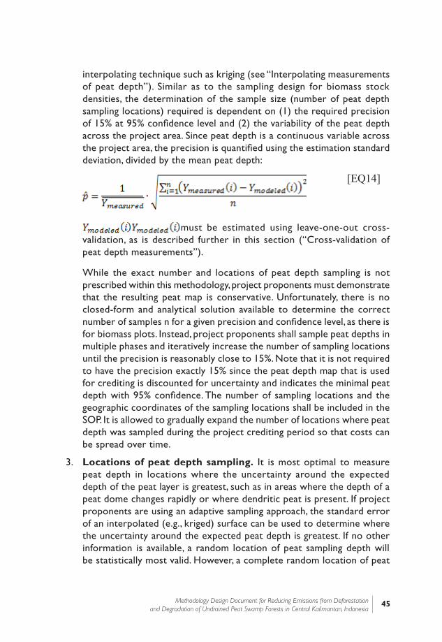
45Methodology Design Document for Reducing Emissions from Deforestation and Degradation of Undrained Peat Swamp Forests in Central Kalimantan, Indonesia
interpolating technique such as kriging (see “Interpolating measurements of peat depth”). Similar as to the sampling design for biomass stock densities, the determination of the sample size (number of peat depth sampling locations) required is dependent on (1) the required precision of 15% at 95% confidence level and (2) the variability of the peat depth across the project area. Since peat depth is a continuous variable across the project area, the precision is quantified using the estimation standard deviation, divided by the mean peat depth:
[EQ14]
must be estimated using leave-one-out cross-validation, as is described further in this section (“Cross-validation of peat depth measurements”).
While the exact number and locations of peat depth sampling is not prescribed within this methodology, project proponents must demonstrate that the resulting peat map is conservative. Unfortunately, there is no closed-form and analytical solution available to determine the correct number of samples n for a given precision and confidence level, as there is for biomass plots. Instead, project proponents shall sample peat depths in multiple phases and iteratively increase the number of sampling locations until the precision is reasonably close to 15%. Note that it is not required to have the precision exactly 15% since the peat depth map that is used for crediting is discounted for uncertainty and indicates the minimal peat depth with 95% confidence. The number of sampling locations and the geographic coordinates of the sampling locations shall be included in the SOP. It is allowed to gradually expand the number of locations where peat depth was sampled during the project crediting period so that costs can be spread over time.
3. Locations of peat depth sampling. It is most optimal to measure peat depth in locations where the uncertainty around the expected depth of the peat layer is greatest, such as in areas where the depth of a peat dome changes rapidly or where dendritic peat is present. If project proponents are using an adaptive sampling approach, the standard error of an interpolated (e.g., kriged) surface can be used to determine where the uncertainty around the expected peat depth is greatest. If no other information is available, a random location of peat sampling depth will be statistically most valid. However, a complete random location of peat

46 Section I: Carbon MRV Methodology
sampling is often practically challenging due to the time it may take to reach a specific location within a dense peat swamp forest. Therefore, it is recommended to use a combination of transects and random locations to select peat depth measuring locations. In addition, peat depth samples must be taken to cover both elevated (anticline) areas and depressed (syncline) areas within a dome. A transect across the peat dome is recommended. Additionally, great care must be taken so that sampling intensity is high where sudden changes in peat depth are expected. Therefore, it is recommended that the sampling locations of peat depth are taken perpendicular to natural boundaries such as rivers as well as the most likely shape of the peat dome.
4. Interpolating measurements of peat depth. Although project proponents are allowed to use any technique to interpolate peat depth in between empirical measurements if it can be demonstrated that the technique is conservative, kriging is a robust technique Kriging refers to a set of special interpolating techniques from geostatistics. Kriging techniques analyze the variance of the difference between measurements, and its relationship to the distance between the sampling locations. The approximation of this relationship by a model curve provides the variogram, which allows the estimation of the three components for all of the points around the measurements: (1) the general trend in the data, (2) the spatially correlated variation and (3) the spatially uncorrelated noise. The predicted surface produced by kriging remains an estimate, for which a standard error can be calculated. Even though ordinary kriging has shown the best results for interpolating peat depth surfaces, project proponents may use block kriging or co-kriging with ancillary data such as elevation, biomass, inundation, distance to streams, etc. if so desired.
5. Cross-validation of peat depth measurements. One particular feature of some interpolating techniques, including kriging, is that at the locations where empirical measurements are available, the modeled value is the same as the empirical value. Therefore, to calculate a truly unbiased estimation variance and calculate the difference
, one must use leave-one-out cross-validation (LOOCV). Leave-one-out cross-validation involves using a single observation from the original sample as the validation data, and the remaining observations as the training data. This is repeated such that each observation in the sample is used once as the validation data. In other words, one has to conduct a separate interpolating analysis for every sampling location, but always with the value of that particular sampling location left out of the input
47Methodology Design Document for Reducing Emissions from Deforestation and Degradation of Undrained Peat Swamp Forests in Central Kalimantan, Indonesia
dataset. The resulting interpolated value is then truly unbiased and can be compared to the empirical measurement by taking the difference
.
Project proponents shall duly record all steps conducted during the kriging analysis and present the variogram and variogram model in the Project Document. In addition, project proponents shall provide a map of (1) the average peat depth, (2) the standard error around each peat depth, and (3) the minimal peat depth with 95% confidence to the auditor. Further in this methodology, values of peat depth at the start of the crediting period are referred to with the following notation:
= Peat depth for location at the start of the credit-ing period [cm]
Finally, project proponents shall create a table showing the amount of land present in 10-cm intervals of minimum peat depth with 95% confidence for every peat conversion stratum (see Table 7). The goal of this table is to provide an overview of how much peat is present in the project area.
Water table measurements must be conducted at the same locations as peat depth measurements. However, it is allowed to have less water table measurement locations than peat depth locations.
Size of area with specified range in peat depth for different conversion strata under the baseline scenario [ha]
Specified range in peat depth [cm]
Conversion to oil palm by burning existing biomass
Conversion to oil palm by removing existing biomass without burning
Clear-cutting followed by drainage and
severe degradation
0-50 2500 2300 2600
50-60 400 300 450
60-70 300 400 400
70-80 200 200 300
80-90 200 200 300
….
48 Section I: Carbon MRV Methodology
1.8.4.3 Calculate Emissions Related to Peat under the Baseline Conditions
Calculate the emissions related to peat under the baseline conditions using the algorithm described below. This algorithm must be used separately for each of the conversion strata identified. Note that, to remain conservative, the land that is converted every year is allocated first in the peat strata with lower peat depth.
Create a data-structure in which all the grid cells developed during kriging have the following data elements:
1. = remaining peat depth for grid cell
2. = year during the crediting period that the grid cell is converted. Set to 0 at the beginning of the project period.
Sort the grid cells from smallest (or no) peat depth to greatest peat depth, and set , the current year of the peat emission model to 1.
Cycle through the following steps for each year of a 100-year period following the project start date:
1. Mark a number of cells for conversion during year so that (1) the total sum of the area of the cells marked for conversion equals the annual conversion rate, (2) the cells are marked from smallest peat depth to greater peat depths, (3) the cells have not been converted yet. Mark cells for conversion by setting to
, the current year of the crediting period.
2. For each of the cells that were converted in the current time step or before, calculate the annual subsidence for every grid cell.
shall be set to the smallest of the following three values:
(1)(2)(3)
If the drainage level is less than 40 cm,
must be set to 0.
49Methodology Design Document for Reducing Emissions from Deforestation and Degradation of Undrained Peat Swamp Forests in Central Kalimantan, Indonesia
[EQ15]
Per (1), the subsidence cannot be greater than the typical subsidence for a given time after conversion as specified in section 8.1.4.1. Per (2), the subsidence cannot be greater than the depth of the remaining peat. Per (3) the actual burn depth is restricted by the depth of the peat layer that is at least 40 cm above the water table. The latter is necessary since it must be considered that only dry peat can burn18. As a consequence, if the drainage level
is less than 40 cm, no burning can occur and
must be set to 0.
Likewise, shall be set to the smallest of the following two values
(1)(2)
[EQ16]
As a consequence, peat subsidence will follow the common pattern after conversion as specified in section 8.1.4.1, and no peat subsidence can happen after the end of the peat depletion time, as required by the VCS AFOLU Requirements.
3. Calculate the new peat depths for the following time period as:
[EQ17]
4. Calculate the emissions from peat oxidation and burning as:
[EQ18]
18] This requirement is analogous to the approved VCS methodology VM0004. The rationale is that the layer of peat 40 cm directly above the lowered water table is too wet to burn due to capillary rise of water in the pore spaces of the peat. Research from temperate peat soils indicates that peat layers remain sufficiently moist up to 40cm above the watertable for averagely decomposed peat material (Gnatowski et al., 2002)

50 Section I: Carbon MRV Methodology
[EQ19]
[EQ20]
Note that for non-plantation landscapes, the peat emission factor will be very specific to the landscape in question and be based on past logging history, land use and water management practices, existing drainage infrastructure, and from a drainage canal. If it is determined that these factors will significantly impact the peat emission factor, project proponents shall re-stratify the area according to these factors so that the emission factor can be assumed to be homogeneous within one stratum.
5. Add one to and go back to step 1 until equals the end of the crediting period.
Calculate the total emissions from peat for year t of the crediting period as:
[EQ21]
Where:
= Number of peat strata [-]
= Number of conversion types [-]
= Drainage level of conversion type at time [cm]
= Minimal depth of peat for peat stratum [cm]

51Methodology Design Document for Reducing Emissions from Deforestation and Degradation of Undrained Peat Swamp Forests in Central Kalimantan, Indonesia
= Adjusted mean bulk density of peat stratum at 95% confidence level The uncertainty in bulk density must be calculated and discounted using the HWCI, see equations [EQ2] through [EQ5] for guidance on how to calculate a HWCI. If the HWCI is less than 15% of the average bulk density in the stratum, no adjustment is necessary. If the HWCI is greater than 15%, the value must be reduced proportionally to the HWCI. [Mg m-3].
= Size of square shaped cell [m2]
= Carbon fraction in peat mass
= Carbon-to-nitrogen (C:N) ratio in peat [-]
= Global warming potential of N2O [-]
= Emission ratio of N2O [-]
= Global warming potential of CH4 [-]
= Emission ratio of CH4 [-]
= Emission from peat from peat stratum at time [tCO2e yr-1]
= Emission from peat from at time [tCO2e]
1.8.5 Determine Emissions from Forest Goods and Services
A forest user is the social group, community, or other entity that is currently extracting any timber or non-timber product (“forest product”).
The PD must contain an identification of the users of the forest in the project area, as well as which forest products the forest users benefiting from.
1. Identification of forest users, forest products
2. Quantitative analysis of the extraction rate of forest products and services
3. Quantitative analysis of the extent to which the extraction of forest goods and services lead to forest degradation
52 Section I: Carbon MRV Methodology
1.8.5.1 Identify Forest Users, Forest Goods, and Forest Services
As indicated above, a forest user is the social group, community, or other entity that is currently extracting any timber or non-timber product. All forest users shall be identified in the Project Document. Forest users may include small-scale farmers, encroachers, hunters, ranchers, loggers, or plantation companies. A qualitative narrative on the broader underlying forces determining the agents’ motivations for extracting forest goods or using forest services must be included in the PD. This qualitative narrative may contain aspects related to population size and pressure, territorial or social conflicts, policies related to subsidies, payments for environmental services, and credits, property and land tenure regime, and market forces influencing land and commodity prices.
1.8.5.2 Determine the Demand of Forest Goods and Usage of Forest Services from the Project Area
1. First, determine the “sphere of influence” of the forest in the project area through participatory rural appraisals. The sphere of influence includes all communities and settlements that are relying on the project area to extract forest products and services. Determining the sphere of influence can be done using local experts, focus group discussions, etc.
2. Next, design a household survey within the sphere of influence to determine (1) the total demand of forest goods and usage of forest services, and (2) the supply of forest goods and usage of forest services from the project area. Determine an appropriate unit of measurement for each forest good and service that is identified.
First calculate the total demand of forest good or service for the households that are in the “sphere of influence”. The demand for forest products and services under the baseline scenario at year 0 shall be set to the average extraction rate from household surveys.
= Extraction of forest good or forest service under the baseline scenario from the project area at the beginning of the crediting period. [(measurement unit)]
Subsequently, calculate the ratio of the demand of forest goods and services from the households in the “sphere of influence” that is supplied by the project area:
53Methodology Design Document for Reducing Emissions from Deforestation and Degradation of Undrained Peat Swamp Forests in Central Kalimantan, Indonesia
= Proportion of the demand for forest good or service in the sphere of influence of the project area that is supplied by the project area. [-]
1.8.5.3 Determine Emission Factors for Forest Goods and Services
Next, the emissions caused by extraction of forest goods and usage of forest services must be quantified. These emissions must be calculated as “emission factors”, relative to the unit of measurement for each forest good and service.
Quantifying these emission factors can be done either based on existing data, if these are available, or based on empirical measurements if no existing data are available.
Within this methodology, these emission factors are referred to as:
= Emission factor for extracting forest good or forest service per unit of measurement [tCO2e (measurement unit)-1]
If the annual emissions for extracting a specific forest good or service represent less than 5% of the total potential emissions from plant organic
matter (calculated as ), this specific forest good or service can be excluded from leakage calculations and monitoring according to the de minimis rules from the VCS.
Finally, project proponents shall determine whether the extraction of forest goods and services will “likely lead to deforestation”. This determination is important as it impacts the monitoring methodology (see Monitoring section). More specifically, leakage of extraction of forest goods and services that likely lead to deforestation must be quantified by monitoring deforestation in leakage belts; leakage of extraction of forest goods and services that does not likely lead to deforestation must be quantified by monitoring extraction rates through social surveys.
To determine whether the extraction of a specific forest good and service will likely lead to deforestation, project proponents shall determine if the extraction of a forest good or service over 1 year leads to a loss of plant carbon of more than 50% and the transition of a averagely stocked forest area to a non-forest area. If these two conditions are present, project proponents
54 Section I: Carbon MRV Methodology
shall label the extraction of this specific forest good or service as “likely leading to deforestation”.
Reporting Requirements, include in PD section 1.7
For each deforestation driver, provide the following information:
1. Name of the forest user group (there may be multiple), the forest goods that are extracted and the forest services that are used.
2. Brief description of the main social, economic, cultural and other relevant features of each forest user, including the broader underlying motivation for forest use.
3. Brief assessment of the most likely development of the population size of the identified forest users in the reference region and project area.
4. Estimate of the extraction rate of forest goods, and usage rate of forest services.
5. Identification of the potential leakage area.
1.9 Project Emissions
1.9.1 Put in Place Agreements to Avoid Conversion
Avoiding legally allowed conversion of the project area requires putting a legally binding agreement in place between the participating communities, landowners, project developers and the relevant government administrative units. These legal agreements are particularly important when the project proponents do not legally own the forest land, and the land-tenure status is unclear or obscured by a complex administrative hierarchy. The project proponents must put in place legally binding agreements with communities and the relevant administration units to avoid the forest conversion through purchasing or securing long-term conservation easements, or the revision of spatial plans and zoning laws. The establishment of these agreements will require funds, which are covered by the benefits from carbon trading. In addition, strengthening and clarifying the land-tenure status is essential to ensure that the extraction of forest goods and services remains sustainable. Obviously, a legal protection of the land is not sufficient for a sound protection of the forest land. It must be complemented with an effective protection, social fencing, or patrolling system.
55Methodology Design Document for Reducing Emissions from Deforestation and Degradation of Undrained Peat Swamp Forests in Central Kalimantan, Indonesia
1.9.2 Identify Project Activities that Prevent Loss of Biomass from Extraction of Forest Goods and Use of Forest Services
Under the project applicability criteria, it is assumed that the biomass in the project area will not decrease under the project scenario. Since local communities may be using the land, some activities must be introduced that focus on increasing the livelihood options of local communities or prevention of leakage through e.g. increasing the land use intensity of already deforested land. Note that ex-post, credits are calculated on all empirically observed changes in stocks. All emissions related to losses of biomass under the project scenario must be discounted from credits.
1.9.2.1 Development of sustainable forest and land use management plans
Forest and land use management plans must be established in a participatory and democratic way. These plans can include the volumes of timber, fuel-wood or NTFP each community can sustainably harvest, the areas of livestock grazing, or the area of forest land that can be converted into settlements or cropland, and where the conversion must take place. The management plans must be based on current and future need for forest products and land. Such plans will increase the efficiency of the current land use and avoid the random conversion of forest patches which can accelerate forest degradation. The plans must be integrated and compatible with the land tenure and use rights. The plans must be long-term or permanent (where possible) in nature.
The management plan is only binding for participating communities and will not affect the drivers of deforestation for which the agents are not participating in the project.
1.9.2.2 Demarcation and Protection of Boundaries
The installation of fences, gates, boundary poles, and signage provides local communities a transparent, recognizable and fixed boundary of the project area. Because legal protection alone may be insufficient to prevent deforestation; often a physical boundary or signage is required to avoid deforestation, and support social fencing and patrolling. The boundaries of the discrete project area parcels must be clearly demarcated to be recognized by potential trespassers of the forest (hunters, loggers, or other encroachers).
The boundaries of the forest must be protected and patrolled. Often, there is a lack of official law enforcers to do this task, while communities are committed to defend their land-tenure and land use rights. Communities can be engaged
56 Section I: Carbon MRV Methodology
in the regular patrolling of the forest area. It must be clarified with the local administration which actions can be taken in case of illegal trespassing (e.g., confiscating chainsaws, alerting local law enforcers, etc.). Improve synergies among local communities, law enforcement and other relevant agencies to support boundary protection. Other project actions include the creation of logistical plans to protect boundaries, social fencing, and the acquisition of equipment (e.g., small motorized vehicles) for patrolling and enforcement.
1.9.2.3 Fire prevention
If forest fires are threatening the project’s forest, specific fire prevention measures could be taken. These include (1) installation of fire breaks, (2) cleaning of the forest from dead wood that can act as fuel for fires, especially around regenerating and young secondary forests, and (3) discouraging or eliminating (if possible) fire-based hunting techniques. Saplings and small trees are particularly vulnerable to forest fires. If this requires cutting down trees, or removing dead wood, the loss of carbon must be accounted for.
1.9.2.4 Providing alternative livelihoods to the agents of deforestation
If deforestation agents can engage in alternative livelihoods that are not based on deforestation, they can secure their income without the need to further clear forests.
1. As many as possible, planned project activities must be carried out by the local communities. Engaging communities in forest patrolling, biomass inventory, fire prevention activities, installation of fences and boundary poles, and assisted natural regeneration activities. These activities will provide employment and a greater financial return flowing to the communities. In addition, the active involvement of the local communities will strengthen the project goals and decrease the risks of project failure.
2. Part of the forest can be made accessible for sustainable eco-tourism, which will create jobs and increase revenue.
3. The sustainable extraction of non-timber forest products can be further developed and commercialized. This includes the harvesting of honey, medicinal plants, fungi, and the extraction of resins. Clear harvesting plans need to be developed to ensure the sustainable extraction of these commodities.
57Methodology Design Document for Reducing Emissions from Deforestation and Degradation of Undrained Peat Swamp Forests in Central Kalimantan, Indonesia
1.9.2.5 Decrease the consumption of fuel-wood
The collection of fuel-wood only leads to forest degradation if it is collected from live trees. A low-intensity collection of fuel-wood from downed dead wood may in fact have a positive effect on forest regeneration by decreasing the potential for forest fires. In cases where the collection of fuel-wood leads to forest degradation, the introduction of fuel-efficient wood-stoves stoves will decrease the need for local consumption fuel-wood (Top et al., 2004). Adoption rates of these alternatives need to be monitored, together with the potential sale of fuel-wood on local markets, which can potentially annul the GHG benefits generated by the alternative stoves. Only fuel-wood gathering for domestic use is allowed in project areas. No commercial sale of fuel-wood gathered in project areas is allowed.
The success of the implementation and on-going maintenance of these activities is critically dependent on the active involvement of all stakeholders in the planning and execution of these project activities. In particular, the local communities must be actively involved. Therefore, project management, advisory, oversight and consultative structures shall be developed to ensure an active involvement of all stakeholders. Through consultation with stakeholders, a transparent mechanism shall be set-up to ensure the equitable distribution of benefits from carbon benefits from the project.
A holistic approach must be taken towards meeting the various resource needs of local communities. For example, rather than excluding local communities from using any forest resources at all (and therefore necessarily forcing them to acquire these resources outside of the project area or purchase these on local or provincial markets, leading to outsource leakage), a sustainable (agro-)forestry management plan must be put in place that can meet local wood and agricultural needs.
1.9.3 Estimate GHG Emissions from Fire Prevention Activities
The carbon loss occurring from the removal of woody biomass from fire prevention activities such as fire breaks must be accounted for19. This includes the emissions from fire breaks cleared by cutting or controlled burning woody biomass. In case controlled burning is used to remove woody biomass, all CH4 emissions related to the burning must be included. The emissions from fire breaks can be calculated by:
19] Emissions from clearing herbaceous vegetation are insignificant.

58 Section I: Carbon MRV Methodology
[EQ22]
where:
= Annual GHG emissions from implementation of fire-preventing actions as REDD project activities. [tCO2-eq yr-1]
= Total annual area of forest stratum that was cleared. [ha yr-1]
= Plant carbon content in forest stratum . It is conservatively assumed that all biomass is removed. [Mg C ha-1 yr-1].
= Annual area of forest stratum that was cleared by controlled burning. [ha yr-1]
= Global Warming Potential for CH4 (IPCC default value = 21 for the first commitment period). [-]
= Emission ratio for CH4 (IPCC default value = 0.012). See Table 3A.1.15 in IPCC GPG-LULUCF (2003). [-]
= Number of forest strata. [-]
1.9.4 Changes in Sinks from Assisted Natural Regeneration Activities
1.9.4.1 Scope and Applicability
This methodology allows specific measures aimed at restoring degraded forest. These ANR activities serve a triple goal: (1) increase the project area’s overall GHG sink strength, (2) reduce activity-shifting, and (3) provide alternative livelihoods to local communities by employing local communities for executing the work. Implementing ANR activities is optional, but shall only be done if all of the following applicability criteria are met.

59Methodology Design Document for Reducing Emissions from Deforestation and Degradation of Undrained Peat Swamp Forests in Central Kalimantan, Indonesia
1. ANR activities occur on degraded forest land within the project area. The conversion of non-forest land into forest land is not allowed under this methodology.
2. Assisted natural regeneration activities must take place on degraded land on which no prior ANR activities have taken place.
3. Assisted natural regeneration activities may consist of thinning, removal of invasive species, enrichment planting, and coppicing.
4. The total size of the areas on which ANR activities are planned must be fixed in the Project Document and the exact location of the ANR activities must be identified before or at the first verification.
Assisted Natural Regeneration shall only be done by implementing one or more of the following measures:
1. Removal of invasive understory species such as ferns or herbs to promote the growth of tree seedlings
2. Thinning of over-stocked and stagnated forest stands to promote radial growth
3. Removal of exotic and/or invasive tree species to promote the growth of native species
4. Stem removal on trees with multiple shoots to promote the growth of a single stem
5. Enrichment planting with trees of biodiversity or social value
A detailed ANR management plan with a detailed description of all activities including their locations, must be included in the PD. An update to the management plan may be submitted at the first verification. However, after first verification, the management plan must be fixed.
1.9.4.2 General Quantification
The calculation of the GHG removals by sinks due to assisted natural regeneration activities is based on the CDM methodology AR-ACM0001 version 3. Wherever possible in this section, notation from AR-ACM0001 version 3 was retained. Combining and annualizing equations (33), (12), (13), and (14) from AR-ACM0001 version 3 yields:
[EQ23]

60 Section I: Carbon MRV Methodology
Where:
= Net anthropogenic greenhouse gas removals due to biomass increase in assisted natural regeneration. [tCO2e]
= Annual change in carbon stocks in all selected carbon pools due to ANR for year . [Mg C yr-1]
= Increase in CO2 emissions from loss of existing woody biomass due to site-preparation (including burning), and/or to competition from forest (or other vegetation) planted as part of the ANR activities. [tCO2e]
= Increase in GHG emissions as a result of the implementation of the proposed ANR activities during year . [tCO2e]
= Baseline greenhouse gas emissions or sources for year . [tCO2e yr-1]
= Total GHG emissions due to leakage for year . [tCO2e yr-1]
1. The procedure for calculating is explained in section 1.9.4.3.
2. The procedure for calculating is explained in section 1.9.4.4.
3. The activity-shifting leakage from ANR activities is included in the total project’s leakage, as explained.
4. The procedure for calculating and is explained in section 1.9.4.5.
1.9.4.3 Estimate Carbon Stock Increase from Biomass
The procedure to calculate the carbon uptake by biomass due to assisted natural regeneration follows the CDM-approved methodology AR-ACM0001 version 3, but adds an explicit uncertainty deduction.
[EQ24]
Where:

61Methodology Design Document for Reducing Emissions from Deforestation and Degradation of Undrained Peat Swamp Forests in Central Kalimantan, Indonesia
= Annual change in carbon stocks in all plant carbon pools due to ANR for year during the crediting period. [Mg C yr-1]
= Number of forest strata. [-]
= Carbon stock change for ANR stratum for year during the crediting period. [Mg C yr-1]
= Discounting factor for the increase in carbon stocks from ANR activities in stratum during time [-]
As stated earlier, is the sum of all plant carbon pools. Similarly as in AR-ACM0001 version 3, changes in dead wood under the project scenario must be conservatively omitted for ex-ante calculations. The aboveground and belowground tree biomass is calculated using the “allometric method” following Equation (22) in AR-ACM0001 version 3:
[EQ25]
Where:
= Amount of land on which ANR activities
are planned under the baseline scenario for year and in stratum . [ha]
and
= Aboveground plant carbon stock density during years and respectively and in stratum . [Mg C ha-1]
= Duration between times 1 and 2. [year]
The uncertainty deduction must be calculated analogously to
and in Equations [EQ10] and [EQ11], but with the carbon content at instead of and the carbon content at instead of :
[EQ26]
If the combined error is smaller is than 0.15, no deduction is applied and the
62 Section I: Carbon MRV Methodology
discounting factor for uncertainty around biomass stock densities is set to 1 as:
[EQ27]
If the combined error is greater than 1, the discounting factor for uncertainty around biomass stock densities is set to 0 as:
[EQ28]
However, if the combined error is greater than 0.15 and smaller than 1, then the discounting factor for uncertainty around biomass stock densities is obtained as:
[EQ29]
Where:
= Combined error in estimated biomass stock density change from time to time within forest stratum . [-]
= Half-width of the 95% confidence interval around the mean carbon stock density of LULC classes of forest stratum at time . [tCO2e ha-1]
Ex-ante, values for biomass densities in ANR areas must be based on pilot projects or data on biomass increases in regenerating forests from the literature. Ex-post, this quantity must to be monitored for actual biomass according to a network of permanent sampling plots. Select a sampling design that can yield a level of precision of ±15% of estimated mean at 95% confidence level. See section 8.1.3.3 for instructions on determining sampling size.
1.9.4.4 Calculate Baseline Emissions or Sinks on Land on which Assisted Natural Regeneration Activities are Planned
Baseline emissions from land on which ANR activities are planned are calculated analogously as for land without ANR activities except for the treatment of forest degradation and regeneration under baseline scenario. To remain conservative, only ANR land under baseline scenario includes transitions between forest and non-forest LULC classes. In addition,

63Methodology Design Document for Reducing Emissions from Deforestation and Degradation of Undrained Peat Swamp Forests in Central Kalimantan, Indonesia
regeneration under the baseline scenario considers using continuous “net annual increments” in Mg C ha-1 yr-1 which shall be specific for the forest strata. This departure from the previous approach for land without ANR is necessary because (1) the combination of the discrete approach to account for changes in biomass by transitions among forest strata for the baseline and carbon accounting approach from AR-ACM0001 version 3 for the scenario will lead to unexpectedly discontinuous GHG benefits from ANR, (2) in cases when forest degradation has been excluded due to low accuracy of remote sensing analysis, this procedure will still assume a baseline regeneration rate. The baseline emissions or sinks on land with ANR can be calculated using the following equation.
[EQ30]
Where:
= Baseline GHG emissions or sources for year . [tCO2e yr-1]
= Carbon fraction of woody material (use a default value of 0.5). [Mg C (Mg DM)-1]
= Number of strata within the project area on which ANR activities are proposed. [-]
= Net annual increment of biomass due to natural regeneration and succession for the “from” class of transition , as reported in section 1.8.3.2. [Mg DM ha-1 yr-1]
= Size of strata within the project area on which ANR activities are proposed for year under the baseline scenario. [ha]
= Number of forest/non-forest transitions among land classes or forest strata, meaning transitions in which either the “from” or the “to” classes are non-forests. [-]
= Discounting factor for uncertainty of LULC classification. [-]
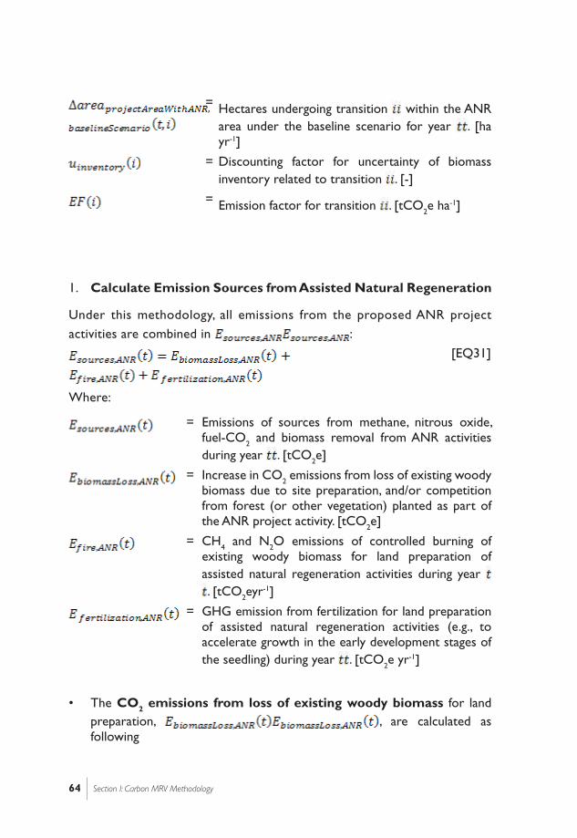
64 Section I: Carbon MRV Methodology
= Hectares undergoing transition within the ANR
area under the baseline scenario for year . [ha yr-1]
= Discounting factor for uncertainty of biomass inventory related to transition . [-]
= Emission factor for transition . [tCO2e ha-1]
1. Calculate Emission Sources from Assisted Natural Regeneration
Under this methodology, all emissions from the proposed ANR project activities are combined in :
[EQ31]
Where:
= Emissions of sources from methane, nitrous oxide, fuel-CO2 and biomass removal from ANR activities during year . [tCO2e]
= Increase in CO2 emissions from loss of existing woody biomass due to site preparation, and/or competition from forest (or other vegetation) planted as part of the ANR project activity. [tCO2e]
= CH4 and N2O emissions of controlled burning of existing woody biomass for land preparation of assisted natural regeneration activities during year . [tCO2eyr-1]
= GHG emission from fertilization for land preparation of assisted natural regeneration activities (e.g., to accelerate growth in the early development stages of the seedling) during year . [tCO2e yr-1]
• The CO2 emissions from loss of existing woody biomass for land preparation, , are calculated as following

65Methodology Design Document for Reducing Emissions from Deforestation and Degradation of Undrained Peat Swamp Forests in Central Kalimantan, Indonesia
[EQ32]
Where:
= Increase in CO2 emissions from loss of existing woody biomass due to site preparation, and/or competition from forest (or other vegetation) planted as part of the ANR project activity. [tCO2e]
= Number of strata within the project area on which ANR activities are proposed. [-]
= Area of biomass removed within ANR stratum during year . [ha]
= Removed carbon content in ANR stratum . [Mg C ha-1 yr-1]
• The CH4 and N2O emissions of burning of existing woody biomass for land preparation, , are calculated as following:
[EQ33]
Where:
= Annual GHG emissions from implementation of fire-preventing actions as REDD project activities. [tCO2e yr-1]
= Number of strata within the project area on which ANR activities are proposed. [-]
= Area of biomass removed within ANR stratum during year using controlled burning . [ha]
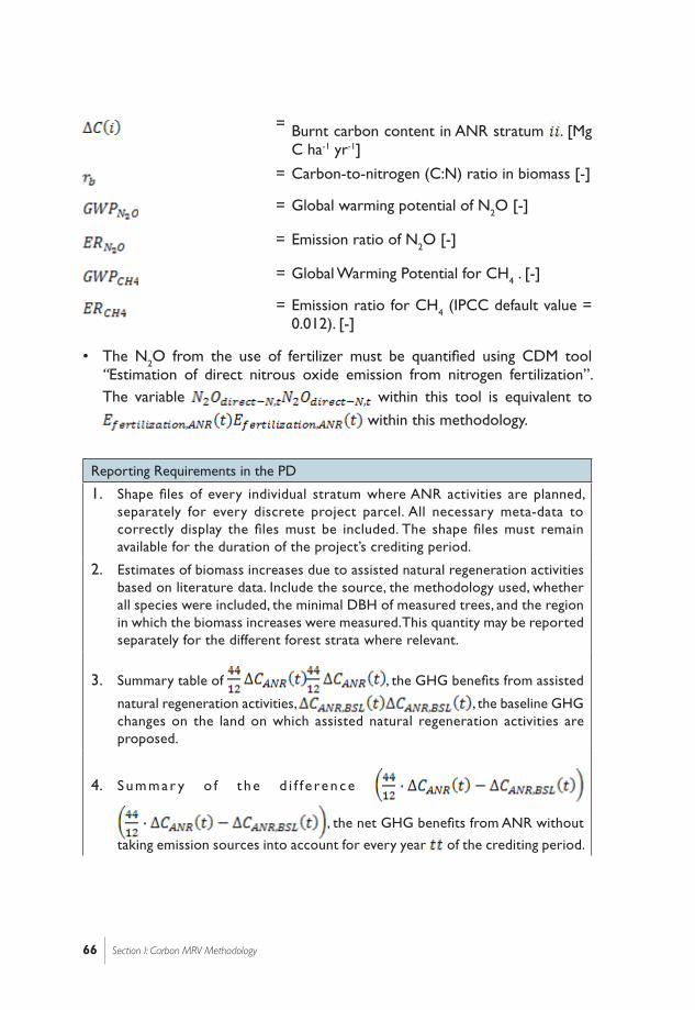
66 Section I: Carbon MRV Methodology
= Burnt carbon content in ANR stratum . [Mg C ha-1 yr-1]
= Carbon-to-nitrogen (C:N) ratio in biomass [-]
= Global warming potential of N2O [-]
= Emission ratio of N2O [-]
= Global Warming Potential for CH4 . [-]
= Emission ratio for CH4 (IPCC default value = 0.012). [-]
• The N2O from the use of fertilizer must be quantified using CDM tool “Estimation of direct nitrous oxide emission from nitrogen fertilization”. The variable within this tool is equivalent to
within this methodology.
Reporting Requirements in the PD
1. Shape files of every individual stratum where ANR activities are planned, separately for every discrete project parcel. All necessary meta-data to correctly display the files must be included. The shape files must remain available for the duration of the project’s crediting period.
2. Estimates of biomass increases due to assisted natural regeneration activities based on literature data. Include the source, the methodology used, whether all species were included, the minimal DBH of measured trees, and the region in which the biomass increases were measured. This quantity may be reported separately for the different forest strata where relevant.
3. Summary table of , the GHG benefits from assisted
natural regeneration activities, , the baseline GHG changes on the land on which assisted natural regeneration activities are proposed.
4. Summar y o f t he d i f f e rence
, the net GHG benefits from ANR without
taking emission sources into account for every year of the crediting period.

67Methodology Design Document for Reducing Emissions from Deforestation and Degradation of Undrained Peat Swamp Forests in Central Kalimantan, Indonesia
5. List of the assumptions, data sources, and other information relevant to the calculation of the emissions for every source related to assisted natural regeneration.
6. Summary table of ,
, for every year
of the crediting period.
7. Summary of , the sum of the GHG emissions
sources related to assisted natural regeneration for every year of the crediting period in the appropriate column of the summary table.
1.9.5 Estimate GHG Emissions from Harvesting
This methodology allows (limited) harvesting of timber from the project area. Allowing harvesting activities undoubtedly (1) increases the attractiveness of a REDD project to participating communities by providing employment and/or access to forest resources, (2) reduces activity-shifting and market leakage, and (3) ensures that harvesting occurs legally, controlled and in a sustainable fashion. An integrated forest management plan or a harvest plan must be developed and all harvesting activities must be carried out according to this plan. The plan must include boundary of areas within a REDD project where harvest activities take place, as well as details of the forest inventory, projected forest growth, projected removal and harvest schedules, harvest methods, and location of harvest activities. In addition, forest management as well as silvicultural activities that aim at enhancing the growth and vigor of the forests inside the harvested areas shall be described in the plan. The integrated forest management plan or harvest plan shall be submitted at validation and may be updated at a baseline update or re-assessment.
If the REDD project is also taking credits from ANR activities, then there should be no overlap of boundaries between ANR areas and harvest areas. In any year, claiming for GHG emissions reduction benefits only from areas where harvesting is taking place is not allowed under this methodology.
1.9.5.1 Determining Long-term Average Carbon
GHG benefits shall be calculated using a carbon stock that never exceeds the long-term average carbon stock in the areas where harvest activities take place. As a consequence, the long-term average carbon stock represents the maximum carbon stock that can be attained in harvesting areas. The long-term
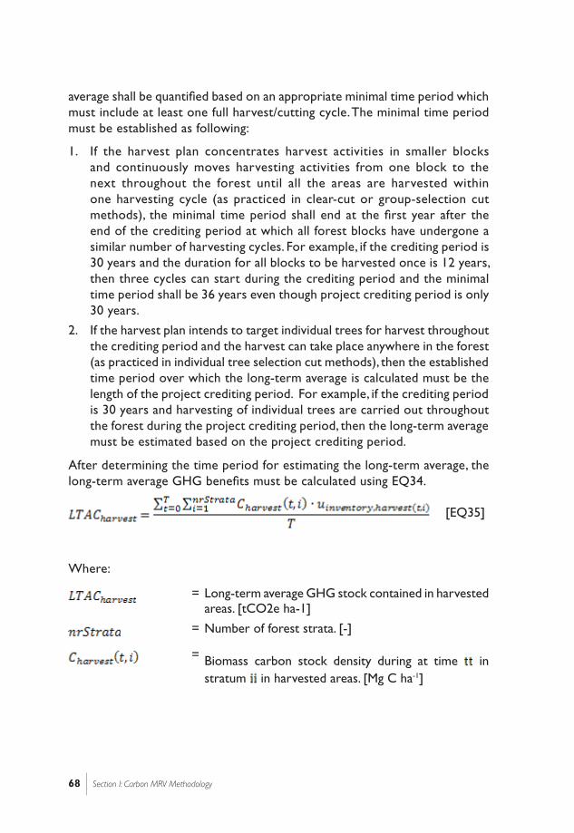
68 Section I: Carbon MRV Methodology
average shall be quantified based on an appropriate minimal time period which must include at least one full harvest/cutting cycle. The minimal time period must be established as following:
1. If the harvest plan concentrates harvest activities in smaller blocks and continuously moves harvesting activities from one block to the next throughout the forest until all the areas are harvested within one harvesting cycle (as practiced in clear-cut or group-selection cut methods), the minimal time period shall end at the first year after the end of the crediting period at which all forest blocks have undergone a similar number of harvesting cycles. For example, if the crediting period is 30 years and the duration for all blocks to be harvested once is 12 years, then three cycles can start during the crediting period and the minimal time period shall be 36 years even though project crediting period is only 30 years.
2. If the harvest plan intends to target individual trees for harvest throughout the crediting period and the harvest can take place anywhere in the forest (as practiced in individual tree selection cut methods), then the established time period over which the long-term average is calculated must be the length of the project crediting period. For example, if the crediting period is 30 years and harvesting of individual trees are carried out throughout the forest during the project crediting period, then the long-term average must be estimated based on the project crediting period.
After determining the time period for estimating the long-term average, the long-term average GHG benefits must be calculated using EQ34.
[EQ35]
Where:
= Long-term average GHG stock contained in harvested areas. [tCO2e ha-1]
= Number of forest strata. [-]
= Biomass carbon stock density during at time in stratum in harvested areas. [Mg C ha-1]
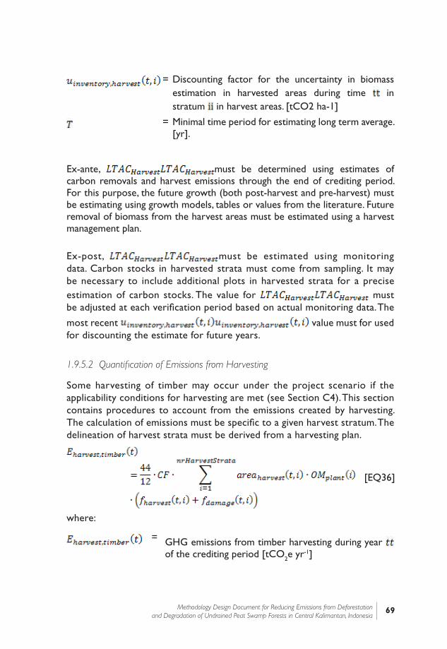
69Methodology Design Document for Reducing Emissions from Deforestation and Degradation of Undrained Peat Swamp Forests in Central Kalimantan, Indonesia
= Discounting factor for the uncertainty in biomass estimation in harvested areas during time in stratum in harvest areas. [tCO2 ha-1]
= Minimal time period for estimating long term average. [yr].
Ex-ante, must be determined using estimates of carbon removals and harvest emissions through the end of crediting period. For this purpose, the future growth (both post-harvest and pre-harvest) must be estimating using growth models, tables or values from the literature. Future removal of biomass from the harvest areas must be estimated using a harvest management plan.
Ex-post, must be estimated using monitoring data. Carbon stocks in harvested strata must come from sampling. It may be necessary to include additional plots in harvested strata for a precise estimation of carbon stocks. The value for must be adjusted at each verification period based on actual monitoring data. The
most recent value must for used for discounting the estimate for future years.
1.9.5.2 Quantification of Emissions from Harvesting
Some harvesting of timber may occur under the project scenario if the applicability conditions for harvesting are met (see Section C4). This section contains procedures to account from the emissions created by harvesting. The calculation of emissions must be specific to a given harvest stratum. The delineation of harvest strata must be derived from a harvesting plan.
[EQ36]
where:
= GHG emissions from timber harvesting during year of the crediting period [tCO2e yr-1]

70 Section I: Carbon MRV Methodology
= Carbon fraction in timber. Use IPCC defaults [-]
= Number of harvest strata [-]
= Area of forest land in harvest stratum that is harvested at time t of the crediting period [ha]
= Live tree biomass in harvest stratum for year [Mg DM ha-1]
= The proportion of biomass removed by harvesting for harvest stratum i and year t. Data for this variable should be obtained from harvest schedule information. Values may be constrained by the timber available for commercial harvest. [-]
= The proportion of additional biomass removed for road/track and landing construction for harvest stratum and year . Data for this variable should be based on regional and local comparative studies and experimental information derived from the local forest industry. [-]
If machinery is used to fell trees, emissions from fossil fuel must be accounted for as well using Approved VCS Module VMD0014 “Estimation of emissions from fossil fuel combustion (E-FFC)”. Emissions from machinery must be included in:
where:
= GHG emissions from fossil fuel during timber harvesting during year t of the crediting period [tCO2e yr-1]
1.9.6 Estimate Emission sources from Community Development Activities
It is good practice to support community development activities as part of the REDD project to minimize any displacement of activities due to the conservation of the forest area. Under this methodology, a number of potential community development activities are allowed (see further for a

71Methodology Design Document for Reducing Emissions from Deforestation and Degradation of Undrained Peat Swamp Forests in Central Kalimantan, Indonesia
detailed specification). Note that the implementation of potential community development activities is optional. However, if community development activities are implemented, they must follow the specification and applicability criteria detailed in this section.
Any significant increase in GHG emissions due to the implementation
of community development activities (
) must be subtracted from the project’s overall GHG emission benefits according to the procedures included within this section. The following sources of GHG emissions are included in this methodology:
[EQ37]
Where:
= Emission sources from community development activities for year of the crediting period. [tCO2e]
= Annual difference in GHG emissions due to increased use of N fertilizer as an agricultural intensification measure for year of the crediting period. [tCO2e]
= Annual difference in GHG emissions due to increased use of flooded rice production systems as agricultural intensification measures for year of the crediting period. [tCO2e]
= Annual difference in GHG emissions by enteric fermentation and manure management from increased animal stocking rates as an agricultural intensification measure for year of the crediting period. [tCO2e]
1.9.6.1 Check Conditions and Quantify Emissions from Intensification of Annual Cropping Systems

72 Section I: Carbon MRV Methodology
1. Scope and Applicability
Intensification of annual crop production systems as a community development activity is optional, but shall only be introduced if all of the following conditions are demonstrated:
1. The agricultural intensification measures are implemented only on land on which annual crop production systems are implemented.
2. The agricultural intensification measures are implemented on land that is already under annual crop production systems at the time of validation.
3. The agricultural intensification measures shall not be implemented on organic soils.
Intensification of annual crop production systems shall only be done by implementing one or more of the following measures:
1. increasing synthetic or organic N inputs
2. the use of fallow crops or shrubs
3. replacing subsistence crops by cash crops
4. replacing low-yielding crop varieties by higher-yielding, or less pest-sensitive crop varieties
5. introduction of irrigation systems
6. introduction of inundated rice production systems
2. Quantification and Monitoring of N2O Emissions
Use CDM tool “Estimation of direct nitrous oxide emission from nitrogen fertilization”20 to quantify emissions. The variable
within this tool is equivalent to within this
methodology. Add annual values of to the summary table of all GHG emissions due to project activities.
All variables that are required to be reported ex-ante by the CDM tool must be included within the PD. All variables that are required to be monitored by the CDM tool must be included within the monitoring plan. For the purpose of this methodology, the following variables are specified in more depth than the specification provided within the CDM tool.
20] http://cdm.unfccc.int/methodologies/ARmethodologies/tools/ar-am-tool-07-v1.pdf

73Methodology Design Document for Reducing Emissions from Deforestation and Degradation of Undrained Peat Swamp Forests in Central Kalimantan, Indonesia
= Mass of synthetic fertilizer type applied in year . is the difference between the synthetic fertilizer applied
during the project in year t and the synthetic fertilizer applied during the baseline. The amount of synthetic fertilizer used per cropping system and per project parcel in the baseline must be quantified and monitored.
=Mass of organic fertilizer type applied in year . is the difference between the organic fertilizer applied during the project in year t and the organic fertilizer applied during the baseline. The amount of organic fertilizer used per cropping system and per project parcel in the baseline must be quantified and monitored.
3. Quantification and Monitoring of CH4 Emissions from Flooded Rice Production
Use GPG 2006 AFOLU Section 5.5 “Methane Emissions From Rice Cultivation” to quantify the methane emissions from flooded rice using the described Tier 1 default emissions factors and scaling factors. The variable
within this tool is equivalent to within this
methodology. Add annual values of to the summary table of all GHG emissions due to project activities.
All variables that are required to be monitored by the CDM tool must be included within the monitoring plan. For the purpose of this methodology, the following variables are specified in more depth than the specification provided within the CDM tool.
Rice production systems must be divided into different sub-units according to the water regime and the number of rice harvests per year, as explained in GPG 2006 AFOLU Section 5.5.1. The following variables from the GPG AFOLU must be quantified ex-ante and monitored for every subunit (notation follows GPG AFOLU section 5.5)
= Annual difference in harvested area of rice for the sub-unit, as defined by conditions , , and , between project and baseline scenario [ha yr-1]. The area of rice cultivation for each condition , , and and for each individual project parcel in the baseline must be quantified using Participatory Rural Appraisals, and re-evaluated regularly.

74 Section I: Carbon MRV Methodology
1.9.6.2 Estimate GHG Emissions from Increased Livestock Stocking Rates,
1. Scope and Applicability
Increasing livestock stocking rates as a community development activity is optional, but shall only be introduced if all of the following conditions are demonstrated:
1. If the proposed activity produces forage to feed livestock, all forage shall have a similar nutritional value and digestibility, and will support only a single livestock group with a single manure management system, cfr. AR-AM0006 applicability criterion (k).
2. If the stocking rate is increase for animals that are already in a zero-grazing system or are moved to a zero-grazing system then the grazing activity that is monitored is the production of fodder, cfr. Displacement of Grazing CDM tool Point 5.
3. Increased stocking rates shall only occur on Identified Forest land, Identified Cropland, Identified Grassland, and Unidentified land, cfr. Displacement of Grazing CDM tool Point 6.
4. Increased stocking rates shall not occur on Settlements, Wetlands, or Other lands – as defined by the GPG LULUCF (i.e. bare soil, rock, ice, and all unmanaged land areas that do not fall into category of forest land, cropland, grassland, settlements or wetlands), cfr. Displacement of Grazing CDM tool Point 5.
Livestock stocking rates shall be increased through either or both of the following measures:
1. Increasing the stocking density of livestock on existing grazing land.
2. Moving of cattle to a zero-grazing system, defined as a system of feeding cattle or other livestock in which forage is brought to animals that are permanently housed instead of being allowed to graze.
75Methodology Design Document for Reducing Emissions from Deforestation and Degradation of Undrained Peat Swamp Forests in Central Kalimantan, Indonesia
2. Quantification and Monitoring of Emissions from Increased Stocking rates
Use the most recent version of approved CDM methodology AR-AM000621, section 8, “Leakage” to determine the CH4 and N2O emissions from livestock, as well as the CDM AR tool “Estimation of GHG emissions related to displacement of grazing activities in A/R CDM project activity”22. The
sum of variable within AR-AM0006 and
within the CDM tool is equivalent to within this methodology.
Use the variables list of default parameters and parameters to be monitored from AR-AM0006 and the CDM tool for displacement of grazing activities. Livestock population increases must be quantified using Participatory Rural Appraisals or peer-reviewed literature, and re-evaluated regularly.
PD Reporting requirements
1. Table with for every year of the crediting period.
2. List of the assumptions, data sources, and other information relevant to the
calculation of the emissions for sources ,
, and from community development activities.
3. A report of , , and for every year of the crediting period.
1.10 Leakage
Leakage has been cited as being a major obstacle for the development of avoided deforestation projects (e.g., Schlamadinger et al., 2005; Miles and Kapos, 2008). However, the mere potential for leakage does not necessarily negate the environmental integrity of an avoided deforestation project. Only in cases where potential leakage cannot be identified and quantified does leakage pose an insurmountable barrier. It is good practice to incorporate
21] http://cdm.unfccc.int/UserManagement/FileStorage/T05CO1LWYIJ7EHD9GBVAKZPUSQ2N8X22] This tool can be found on http://cdm.unfccc.int/methodologies/ARmethodologies/tools/ar-am-tool-09-v2.pdf. This tool has
been approved for A/R CDM projects, but is applicable to REDD projects. All references to “A/R CDM” within this tool should be interpreted as “REDD”.
76 Section I: Carbon MRV Methodology
measures to minimize leakage (see section 1.9.1). The leakage emissions that cannot be avoided must be subtracted from the emission reductions. Under this methodology, leakage is estimated ex-ante, but actual NERs are based on actual leakage calculated with project monitoring data. Leakage does not only occur on forest land outside of the project area, but also on non-forest land, such as woodlands or grassland.
1.10.1 Leakage as a result of the displacement of planned conversion activities
An avoided planned deforestation project may shift deforesting activities from the project area to an area outside the project area, causing leakage. Because the quantification of activity shifting leakage is dependent upon the identification of deforestation agents, two different scenarios are discussed for quantification of activity shifting leakage.
1. When the deforestation agents can be identified, it must be demonstrated that the management plans and/or land-use designations of the deforestation agents’ other lands (which shall be identified by location) have not materially changed as a result of the project (e.g., the deforestation agent has not designated new lands as timber concessions). If the deforestation agents were found to have acquired new lands for planned conversion, the area of the new lands shall be used as the basis for calculating leakage. Unless project proponents can demonstrate that newly acquired lands have no peat or lower peat lands, by default, the leakage must be considered to be happening on areas containing peat at the same proportion as that of the project area. Project proponents can simply calculate emissions from leakage by multiplying the gross emission reductions from the project per unit area for a given year with the area of conversion occurring in the newly acquired lands.
2. When the specific deforestation agent cannot be identified, and only the “most likely” deforestation agent is identified, the areas allotted for land conversion within the administrative level that has jurisdiction over land sanctioning or within the ownership/usage right of the same deforestation agent must be monitored. If the sum of this area increases during the crediting period, compared to historical values, project proponents must deduct the emissions related to this increase from the NERs. More specifically, the following steps must be followed:a. Determine which administration has jurisdiction over the land
sanctioning for the identified conversion scenarios in the area in which the project is located.

77Methodology Design Document for Reducing Emissions from Deforestation and Degradation of Undrained Peat Swamp Forests in Central Kalimantan, Indonesia
b. Acquire all available data on historical areas of conversion for land sanctioned for conversion for each of the conversion strata found in the project area representing for a period of 10 years before the start of the crediting period. All available data shall be used. The source of the data shall be made available to the auditor so that it can be verified that all of the available data is effectively included. Note that it is acceptable to have gaps in the available data.
c. Calculate the average annual amount of area allotted for the specific conversion using all of the available data collected in the previous step.
d. During monitoring, the size of the area that has been sanctioned for the identified conversion scenario(s) by the relevant administrative jurisdiction must be acquired. Calculate the average and standard deviation of the difference of the conversion area with each conversion rate before the project. Using a one-sided t-test, determine whether the actual area allotted for land conversion is not more than 15% of the project area with 95% confidence. Verify that the power of the t-test is at least 80%.• If the statistical power is at least 0.80 and the result of the t-test
shows that the increase in the area allotted for conversion is smaller than 15% of the project area, leakage is assumed to be insignificant.
• If the statistical power is inadequate or the t-test indicates that the increase in the area allotted for conversion is greater than 15% of the project area, the leakage area is equal to the average difference between the monitored conversion and the pre-project conversion unless it can be justified that the observed increase in conversion is unrelated to the project. Justification can be provided by
• Increases in conversion of similar native forest systems far away from the project area and reference region or even globally.
• Analysis of the actual driver of the increase in conversion.
• Peer-reviewed literature and independent sources indicating the causes of the increase in deforestation.
When the leakage area, determined using the procedures is greater than the size of the project area, it should be capped to the size of the project area.
Calculation Example 1
(1) Only data on conversion for 5 out of the 10 years preceding the start of the crediting period are available. The areas are: 40620, 41200, 41025, 40200, and 40650 ha.
78 Section I: Carbon MRV Methodology
(2) The project area is 5000 ha
(3) The area that was converted after the start of the project is 41050
The average increase in deforestation rate is 311 ha, and the standard deviation is 390 ha. A 15% of the project area equals 750. The zero hypothesis of the t-test is: the true increase in deforestation (estimated as 311 ha) is greater or equal than 15% of the project area (i.e., 750 ha). The alternative hypothesis is: the true increase in deforestation is less than 15% of the project area. The p-value of this t-test is 3%, indicating that the alternative hypothesis is true and that leakage is potentially insignificant. However, a test of the power of the test indicates that the power is only 67%. Therefore, the t-test has insufficient power to conclude anything and leakage has to be assumed to be 311 ha.
Calculation Example 2
(1) Data on conversion for 7 out of the 10 years preceding the start of the crediting period are available. The areas are: 40620, 41200, 41025, 40200, and 40650 ha.
(2) Same project area as in case 1: 5000 ha
(3) Same area that was converted after the start of the project as in case 1: 41050
Now the p-value of the same t-test is 0.005, and the power is 95%. As a consequence, the alternative hypothesis (“the true increase in deforestation is less than 15% of the project area”) can be adopted and leakage can be considered insignificant.
1.10.2 Leakage as a result of the displacement of forest products
Leakage as a result of the displacement of forest products such as timber and fuelwood is considered insignificant as the displacement of forest products would have happened under the baseline scenario (conversion of the project area) as well.
PD Reporting requirements
1. Justification and assumptions made to obtain the leakage cancellation rates
for every geographically constrained deforestation
driver .
79Methodology Design Document for Reducing Emissions from Deforestation and Degradation of Undrained Peat Swamp Forests in Central Kalimantan, Indonesia
2. Summarizing table of the leakage cancellation rates
for each deforestation driver .
3. Table with
and , the total relative impact of leakage on the decrease in GHG emissions due to project activities for deforestation and forest degradation respectively,
together with and , for every
year of the crediting period.
4. Decision criteria, data sources, field information, and maps used to demarcate the leakage belt.
5. A map of the leakage area with a clear indication which areas were excluded due to inaccessibility.
6. Table with
,
,
and
the absolute deforestation and forest degradation rates for the project and
leakage areas under baseline and project scenarios for every year of the crediting period.
7. Table with all land transitions for the leakage area under the baseline and project scenarios for every year of the next baseline validation period.
8. Justification and assumptions made to obtain the leakage cancellation
rates for every geographically unconstrained
deforestation driver .
1.11 Summary of GHG Emission Reduction and/or Removals
1.11.1 Estimate Changes in Carbon in Long-lived Wood Products
This methodology considers the carbon in long-lived wood products ( sequestered for over 100 year as permanently sequestered carbon. The
net change in carbon in long-lived wood products is calculated by subtracting
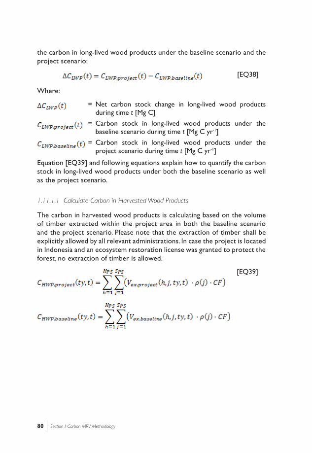
80 Section I: Carbon MRV Methodology
the carbon in long-lived wood products under the baseline scenario and the project scenario:
[EQ38]
Where:
= Net carbon stock change in long-lived wood products during time t [Mg C]
= Carbon stock in long-lived wood products under the baseline scenario during time t [Mg C yr-1]
= Carbon stock in long-lived wood products under the project scenario during time t [Mg C yr-1]
Equation [EQ39] and following equations explain how to quantify the carbon stock in long-lived wood products under both the baseline scenario as well as the project scenario.
1.11.1.1 Calculate Carbon in Harvested Wood Products
The carbon in harvested wood products is calculating based on the volume of timber extracted within the project area in both the baseline scenario and the project scenario. Please note that the extraction of timber shall be explicitly allowed by all relevant administrations. In case the project is located in Indonesia and an ecosystem restoration license was granted to protect the forest, no extraction of timber is allowed.
[EQ39]

81Methodology Design Document for Reducing Emissions from Deforestation and Degradation of Undrained Peat Swamp Forests in Central Kalimantan, Indonesia
Where:
and
= Total carbon stock in long-lived wood products within the project boundary forclass of wood products at time in the project and baseline scenario, respectively [Mg C yr-1]
and
= The volume of timber extracted from within the project boundary during harvest by species and wood product class at time in the
project and baseline scenario, respectively [m3 yr-1].
= Wood density of species [Mg m-3]
= 1, 2, 3, …, number of harvests [-]
= 1, 2, 3, …, harvested tree species [-]
= Wood product class – defined here as sawn wood (sw), wood-based panels (wp), other industrial roundwood (oir), and paper and paper board (ppb).
= Carbon fraction of wood [Mg C (Mg DM)-1] (default value = 0.5)
1. Under the baseline scenario, must be calculated as the sum of timber collected for domestic and commercial purposes. The uncertainty around the estimates of collected timber must be estimated and/or justified with appropriate methods, such as reported uncertainties from scientific literature, or calculated uncertainties when social assessments are used. In situations when uncertainty cannot be estimated, the most conservative estimate must be used.
2. For the ex-ante project case, , must be calculated using the procedures in section 1.9.1.
3. Ex-post, must be monitored and quantified using forest operation records (i.e., log books kept as part of forest management plan). The uncertainty around the monitored volume of timber must be explicitly reported.

82 Section I: Carbon MRV Methodology
In case the uncertainty, as quantified by the half-width of the 95% confidence interval, is less than 15% of the volume of timber extracted, no adjustment for uncertainty must be applied. If, however, the uncertainty is greater than 15% of the volume of timber extracted, must
be adjusted upwards with its associated uncertainty and
must be adjusted downwards with its associated uncertainty using the following equation.
[EQ40]
All parameters are as defined previously.
1.11.1.2 Calculate the Carbon in Long-lived Wood Products
Carbon in long-lived wood products is defined as being sequestered for at least 100 years. Instead of tracking annual emissions through retirement, burning and decomposition, the methodology calculates the proportion of wood products that have not been emitted to the atmosphere 100 years after harvest and assumes that this proportion is permanently sequestered. All factors are derived from Winjum et al. (1998).
[EQ41]

83Methodology Design Document for Reducing Emissions from Deforestation and Degradation of Undrained Peat Swamp Forests in Central Kalimantan, Indonesia
Where:
and
= Carbon stock of long-lived wood products at time t in the project and baseline scenario, respectively. [Mg C]
and
= Total biomass carbon harvested within the project boundary by wood class in the project and baseline scenario, respectively [Mg C]
Fraction of carbon in harvested wood products that are emitted immediately because of mill inefficiency for wood product class . This can be estimated by multiplying the applicable fraction to the total amount of carbon in different harvested wood product category. The default applicable fraction is 24% and 19% respectively for developing and developed countries (Winjum et al. 1998).
= Proportion of short lived products. These fractions are 0.2, 0.1, 0.4 and 0.3 respectively for wood product class , being sawnwood, wood-based panel, paper and paper boards or other industrial round woods as described in Winjum et al. (1998). The methodology assumes that all other classes of wood products are emitted within 5 years.
= Fraction of carbon that will be emitted to the atmosphere between 5 and 100 years of harvest for wood product class . See Table 8. [-]
= 1, 2, 3…..t years elapsed since the start of the project. [yr]
= Wood product class – defined here as sawnwood (sw), wood-based panels (wp), other industrial round wood (oir), and paper and paper board (ppb)

84 Section I: Carbon MRV Methodology
Wood product categoryForest region
Boreal Temperate Tropical
Sawnwood 0.378 0.613 0.850
Wood base panel 0.613 0.850 0.977
Other industrial round wood 0.850 0.977 0.999
Paper and paperboard 0.378 0.613 0.999Source: Winjum et al. 1998
The values in this table represent emissions taking place between year 5 and 100, and therefore represent 95 years.
1.11.2 Summarize the projected land use change
1. Present a table with the total deforestation and degradation rates under the baseline and project scenarios for the project area and leakage area for every year of the project duration.
2. Present tables with the LULC class and forest-strata specific land transitions for the project and leakage area under the baseline and project scenarios.
3. Subtract the land transition changes under the baseline scenario from the changes under the project scenario and multiply with the difference of the appropriate emission factor and baseline net annual increment and apply all uncertainty discounting factors.
4. Calculate the difference the net GHG benefits from ANR without taking emission sources into account for every year of the crediting period.
5. Test the significance of increase in GHG emission from project activities using the CDM A/R methodological tool “Tool for testing significance of GHG emissions in A/R CDM project activities” and omit insignificant emissions from NER calculation.
1.11.3 Calculate Ex-ante NERs
Use Equation [EQ42] to estimate the ex-ante NERs; only use the significant GHG sources as determined in step 2. Prepare a table with all the individual terms of Equation [EQ42]. Calculate the ex-ante NERs for every year of the
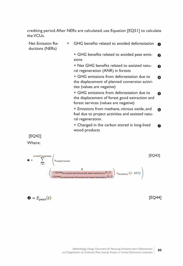
85Methodology Design Document for Reducing Emissions from Deforestation and Degradation of Undrained Peat Swamp Forests in Central Kalimantan, Indonesia
crediting period. After NERs are calculated, use Equation [EQ51] to calculate the VCUs.
Net Emission Re-ductions (NERs)
= GHG benefits related to avoided deforestation
+ GHG benefits related to avoided peat emis-sions+ Net GHG benefits related to assisted natu-ral regeneration (ANR) in forests+ GHG emissions from deforestation due to the displacement of planned conversion activi-ties (values are negative)+ GHG emissions from deforestation due to the displacement of forest good extraction and forest services (values are negative)+ Emissions from methane, nitrous oxide, and fuel due to project activities and assisted natu-ral regeneration.+ Changed in the carbon stored in long-lived wood products
[EQ42]
Where:
[EQ43]
[EQ44]
Project Scenario
Baseline Scenario

86 Section I: Carbon MRV Methodology
[EQ45]
In case: [EQ46]
In case the inequality above does not hold, (4) shall be:
[EQ47]
[EQ48]
[EQ49]
[EQ50]
Variable Description
Net emission reductions during year . Section 1.9.4.3
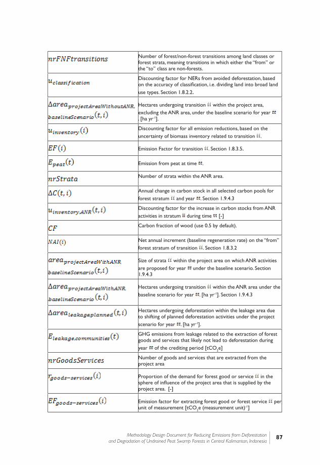
87Methodology Design Document for Reducing Emissions from Deforestation and Degradation of Undrained Peat Swamp Forests in Central Kalimantan, Indonesia
Number of forest/non-forest transitions among land classes or forest strata, meaning transitions in which either the “from” or the “to” class are non-forests.
Discounting factor for NERs from avoided deforestation, based on the accuracy of classification, i.e. dividing land into broad land use types. Section 1.8.2.2.
Hectares undergoing transition within the project area, excluding the ANR area, under the baseline scenario for year . [ha yr-1].
Discounting factor for all emission reductions, based on the uncertainty of biomass inventory related to transition .
Emission Factor for transition . Section 1.8.3.5.
Emission from peat at time .
Number of strata within the ANR area.
Annual change in carbon stock in all selected carbon pools for forest stratum and year . Section 1.9.4.3
Discounting factor for the increase in carbon stocks from ANR activities in stratum during time [-]
Carbon fraction of wood (use 0.5 by default).
Net annual increment (baseline regeneration rate) on the “from” forest stratum of transition . Section 1.8.3.2
Size of strata within the project area on which ANR activities are proposed for year under the baseline scenario. Section 1.9.4.3
Hectares undergoing transition within the ANR area under the baseline scenario for year . [ha yr-1]. Section 1.9.4.3
Hectares undergoing deforestation within the leakage area due to shifting of planned deforestation activities under the project scenario for year . [ha yr-1].
GHG emissions from leakage related to the extraction of forest goods and services that likely not lead to deforestation during year of the crediting period [tCO2e]
Number of goods and services that are extracted from the project area
Proportion of the demand for forest good or service in the sphere of influence of the project area that is supplied by the project area. [-]
Emission factor for extracting forest good or forest service per unit of measurement [tCO2e (measurement unit)-1]

88 Section I: Carbon MRV Methodology
Demand for forest good or forest service under the baseline scenario at year in the selected unit of measurement per household. [(measurement unit)]
Reduction in demand for forest good or forest service due to project activities. [(measurement unit)]
Emissions from sources of methane, nitrous oxide or fuel-CO2 from activities within the project area for year .
Emissions from sources of methane, nitrous oxide or fuel-CO2 from community development activities for year . Emission sources within the leakage area are included in Table 1. Section 1.9.6.
Emissions of sources of methane, nitrous oxide or fuel-CO2 from assisted natural regeneration activities for year . Section 1.9.4.5
GHG emissions from timber harvesting during year t of the crediting period [tCO2e yr-1]
GHG emissions from fossil fuel during timber harvesting during year t of the crediting period [tCO2e yr-1]
VCUs are then calculated by discounting the NERs according to the buffer withholding percentage as determined using the VCS tool for AFOLU non-permanence risk analysis and buffer determination.
[EQ51]
where:
= Voluntary Carbon Units. [tCO2e]
= the buffer withholding percentage according to the VCS tool for AFOLU non-permanence risk analysis and buffer determination. [-]
= Net Emission Reductions. [tCO2e]
Cumulative credits from ANR activities must account for less than 50% of the cumulative credits generated by the project. For every year of the crediting period, divide from [EQ21] by the total NERS, and confirm that the result is less than 50%. Note that NERs are only validated for a period of ten years after validation, but must be reported for the entire crediting period.
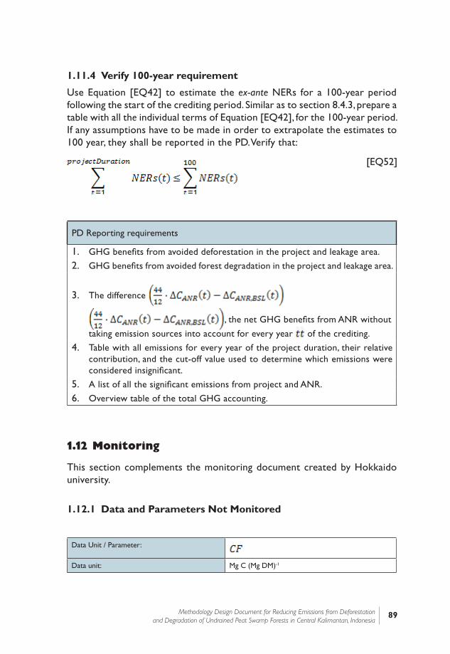
89Methodology Design Document for Reducing Emissions from Deforestation and Degradation of Undrained Peat Swamp Forests in Central Kalimantan, Indonesia
1.11.4 Verify 100-year requirement
Use Equation [EQ42] to estimate the ex-ante NERs for a 100-year period following the start of the crediting period. Similar as to section 8.4.3, prepare a table with all the individual terms of Equation [EQ42], for the 100-year period. If any assumptions have to be made in order to extrapolate the estimates to 100 year, they shall be reported in the PD. Verify that:
[EQ52]
PD Reporting requirements
1. GHG benefits from avoided deforestation in the project and leakage area.
2. GHG benefits from avoided forest degradation in the project and leakage area.
3. The difference
, the net GHG benefits from ANR without
taking emission sources into account for every year of the crediting.
4. Table with all emissions for every year of the project duration, their relative contribution, and the cut-off value used to determine which emissions were considered insignificant.
5. A list of all the significant emissions from project and ANR.
6. Overview table of the total GHG accounting.
1.12 Monitoring
This section complements the monitoring document created by Hokkaido university.
1.12.1 Data and Parameters Not Monitored
Data Unit / Parameter:
Data unit: Mg C (Mg DM)-1

90 Section I: Carbon MRV Methodology
Description: Carbon fraction of dry matter in biomass
Source of data: IPCC GPG-LULUCF (2003)
Justification of choice of data or description of measurement methods and procedures applied:
Use default value of 0.5
Any comment:
Data Unit / Parameter:
Data unit: cm
Description: Annual maximal subsidence due to oxidation for
stratum at time
Source of data: Measurement by project proponent or recent literature such as Couwenberg et al. 2010.
Justification of choice of data or description of measurement methods and procedures applied:
The maximal peat subsidence scenario details how much peat can maximally disappear (in cm yr-1) for every year after the conversion. This rate is maximal in the sense that the peat layer never gets depleted beyond this.
Any comment:
Data Unit / Parameter:
Data unit: cm
Description: Annual maximal subsidence due to burning for
stratum at time
Source of data: Measurement by project proponent or recent literature such as Couwenberg et al. 2010.
Justification of choice of data or description of measurement methods and procedures applied:
The maximal peat subsidence scenario details how much peat can maximally disappear (in cm yr-1) for every year after the conversion. This rate is maximal in the sense that the peat layer never gets depleted beyond this.
Any comment:
Data Unit / Parameter:
Data unit: cm yr-3
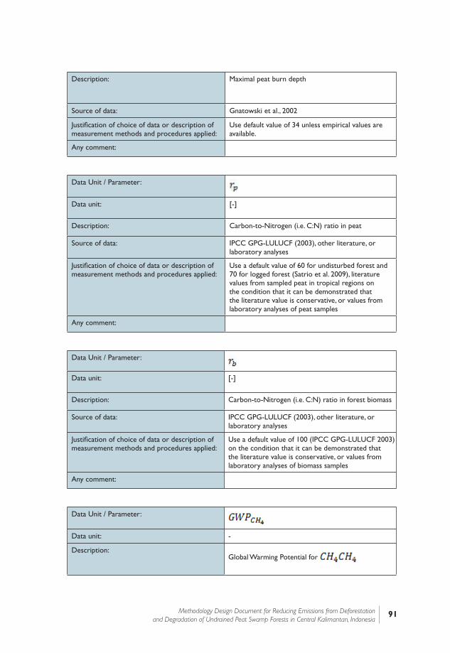
91Methodology Design Document for Reducing Emissions from Deforestation and Degradation of Undrained Peat Swamp Forests in Central Kalimantan, Indonesia
Description: Maximal peat burn depth
Source of data: Gnatowski et al., 2002
Justification of choice of data or description of measurement methods and procedures applied:
Use default value of 34 unless empirical values are available.
Any comment:
Data Unit / Parameter:
Data unit: [-]
Description: Carbon-to-Nitrogen (i.e. C:N) ratio in peat
Source of data: IPCC GPG-LULUCF (2003), other literature, or laboratory analyses
Justification of choice of data or description of measurement methods and procedures applied:
Use a default value of 60 for undisturbed forest and 70 for logged forest (Satrio et al. 2009), literature values from sampled peat in tropical regions on the condition that it can be demonstrated that the literature value is conservative, or values from laboratory analyses of peat samples
Any comment:
Data Unit / Parameter:
Data unit: [-]
Description: Carbon-to-Nitrogen (i.e. C:N) ratio in forest biomass
Source of data: IPCC GPG-LULUCF (2003), other literature, or laboratory analyses
Justification of choice of data or description of measurement methods and procedures applied:
Use a default value of 100 (IPCC GPG-LULUCF 2003) on the condition that it can be demonstrated that the literature value is conservative, or values from laboratory analyses of biomass samples
Any comment:
Data Unit / Parameter:
Data unit: -
Description:Global Warming Potential for
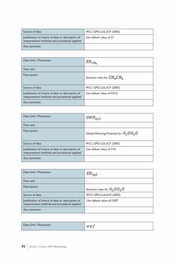
92 Section I: Carbon MRV Methodology
Source of data: IPCC GPG-LULUCF (2003)
Justification of choice of data or description of measurement methods and procedures applied:
Use default value of 21
Any comment:
Data Unit / Parameter:
Data unit: -
Description:Emission ratio for
Source of data: IPCC GPG-LULUCF (2003)
Justification of choice of data or description of measurement methods and procedures applied:
Use default value of 0.012
Any comment:
Data Unit / Parameter:
Data unit: -
Description:Global Warming Potential for
Source of data: IPCC GPG-LULUCF (2003)
Justification of choice of data or description of measurement methods and procedures applied:
Use default value of 310
Any comment:
Data Unit / Parameter:
Data unit: -
Description:Emission ratio for
Source of data: IPCC GPG-LULUCF (2003)
Justification of choice of data or description of measurement methods and procedures applied:
Use default value of 0.007
Any comment:
Data Unit / Parameter:

93Methodology Design Document for Reducing Emissions from Deforestation and Degradation of Undrained Peat Swamp Forests in Central Kalimantan, Indonesia
Data unit:
Description: Fraction of carbon in harvested wood products that are emitted immediately because of mill inefficiency
for wood product class .
Source of data: Winjum et al. 1998
Justification of choice of data or description of measurement methods and procedures applied:
This can be estimated by multiplying the applicable fraction to the total amount of carbon in different harvested wood product category. The default applicable fraction is 24% and 19% respectively for developing and developed countries.
Any comment:
Data Unit / Parameter:
Data unit:
Description: Proportion of short lived products.
Source of data: Winjum et al. (1998)
Justification of choice of data or description of measurement methods and procedures applied:
These fractions are 0.2, 0.1, 0.4 and 0.3 respectively
for wood product class , being sawnwood, wood-based panel, paper and paper boards or other industrial round woods as described in Winjum et al. (1998).
Any comment: The methodology assumes that all other classes of wood products are emitted within 5 years.
Data Unit / Parameter:
Data unit: [-]
Description: Fraction of carbon that will be emitted to the atmosphere between 5 and 100 years of harvest for
wood product class .
Source of data: Winjum et al. (1998)
Justification of choice of data or description of measurement methods and procedures applied:
Select one of the values in Table 1.9.
Any comment:
Data Unit / Parameter:
Data unit: [Mg m-3]
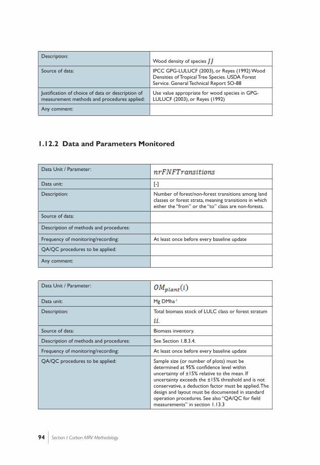
94 Section I: Carbon MRV Methodology
Description:Wood density of species
Source of data: IPCC GPG-LULUCF (2003), or Reyes (1992) Wood Densities of Tropical Tree Species. USDA Forest Service. General Technical Report SO-88
Justification of choice of data or description of measurement methods and procedures applied:
Use value appropriate for wood species in GPG-LULUCF (2003), or Reyes (1992)
Any comment:
1.12.2 Data and Parameters Monitored
Data Unit / Parameter:
Data unit: [-]
Description: Number of forest/non-forest transitions among land classes or forest strata, meaning transitions in which either the “from” or the “to” class are non-forests.
Source of data:
Description of methods and procedures:
Frequency of monitoring/recording: At least once before every baseline update
QA/QC procedures to be applied:
Any comment:
Data Unit / Parameter:
Data unit: Mg DMha-1
Description: Total biomass stock of LULC class or forest stratum
.
Source of data: Biomass inventory.
Description of methods and procedures: See Section 1.8.3.4.
Frequency of monitoring/recording: At least once before every baseline update
QA/QC procedures to be applied: Sample size (or number of plots) must be determined at 95% confidence level within uncertainty of ±15% relative to the mean. If uncertainty exceeds the ±15% threshold and is not conservative, a deduction factor must be applied. The design and layout must be documented in standard operation procedures. See also “QA/QC for field measurements” in section 1.13.3
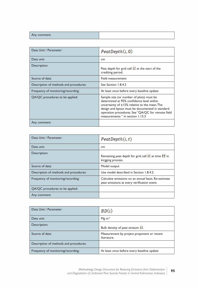
95Methodology Design Document for Reducing Emissions from Deforestation and Degradation of Undrained Peat Swamp Forests in Central Kalimantan, Indonesia
Any comment:
Data Unit / Parameter:
Data unit: cm
Description:Peat depth for grid cell at the start of the crediting period.
Source of data: Field measurement
Description of methods and procedures: See Section 1.8.4.2
Frequency of monitoring/recording: At least once before every baseline update
QA/QC procedures to be applied: Sample size (or number of plots) must be determined at 95% confidence level within uncertainty of ±15% relative to the mean. The design and layout must be documented in standard operation procedures. See “QA/QC for remote field measurements ” in section 1.13.3
Any comment:
Data Unit / Parameter:
Data unit: cm
Description:Remaining peat depth for grid cell at time in kirgging process.
Source of data: Model output
Description of methods and procedures: Use model described in Section 1.8.4.2.
Frequency of monitoring/recording: Calculate emissions on an annual basis. Re-estimate peat emissions at every verification event.
QA/QC procedures to be applied:
Any comment:
Data Unit / Parameter:
Data unit: Mg m-3
Description:Bulk density of peat stratum .
Source of data: Measurement by project proponent or recent literature.
Description of methods and procedures:
Frequency of monitoring/recording: At least once before every baseline update
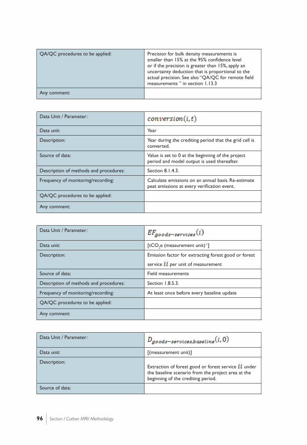
96 Section I: Carbon MRV Methodology
QA/QC procedures to be applied: Precision for bulk density measurements is smaller than 15% at the 95% confidence level or if the precision is greater than 15%, apply an uncertainty deduction that is proportional to the actual precision. See also “QA/QC for remote field measurements ” in section 1.13.3
Any comment:
Data Unit / Parameter:
Data unit: Year
Description: Year during the crediting period that the grid cell is converted.
Source of data: Value is set to 0 at the beginning of the project period and model output is used thereafter.
Description of methods and procedures: Section 8.1.4.3.
Frequency of monitoring/recording: Calculate emissions on an annual basis. Re-estimate peat emissions at every verification event.
QA/QC procedures to be applied:
Any comment:
Data Unit / Parameter:
Data unit: [tCO2e (measurement unit)-1]
Description: Emission factor for extracting forest good or forest
service per unit of measurement
Source of data: Field measurements
Description of methods and procedures: Section 1.8.5.3.
Frequency of monitoring/recording: At least once before every baseline update
QA/QC procedures to be applied:
Any comment:
Data Unit / Parameter:
Data unit: [(measurement unit)]
Description:Extraction of forest good or forest service under the baseline scenario from the project area at the beginning of the crediting period.
Source of data:

97Methodology Design Document for Reducing Emissions from Deforestation and Degradation of Undrained Peat Swamp Forests in Central Kalimantan, Indonesia
Description of methods and procedures: See section 1.8.5.2
Frequency of monitoring/recording: At least once before every baseline update
QA/QC procedures to be applied:
Any comment:
Data Unit / Parameter:
Data unit: [-]
Description: Proportion of the demand for forest good or
service in the sphere of influence of the project area that is supplied by the project area. [-]
Source of data:
Description of methods and procedures: See section 1.8.5.2
Frequency of monitoring/recording: At validation only
QA/QC procedures to be applied:
Any comment:
Data Unit / Parameter:
Data unit: Mg C ha-1 yr-1
Description: Net annual increment of biomass for forest stratum
under the baseline scenario.
Source of data: Estimate within the biomass inventory plots outside of the ANR area
Description of methods and procedures: Only to be included if ANR activities are implemented (Lower-ranked options may only be used if higher-ranked options are not available).
• Values measured by the project proponents in the project area
• National or local growth curves and tables
• Values from peer-reviewed literature
Values from GPG-LULUCF Table 3A.1.5.
Frequency of monitoring/recording: At least once before every verification
QA/QC procedures to be applied: See “QA/QC for remote field measurements ” in section 1.13.3
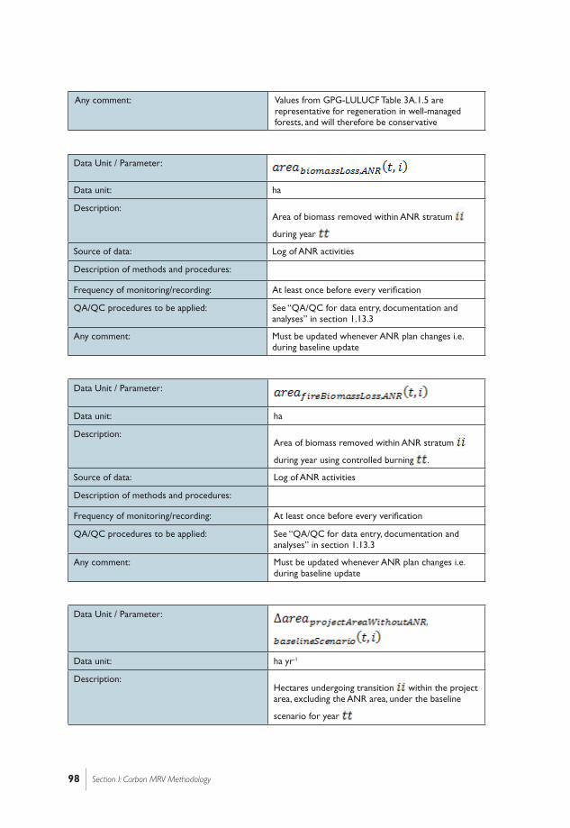
98 Section I: Carbon MRV Methodology
Any comment: Values from GPG-LULUCF Table 3A.1.5 are representative for regeneration in well-managed forests, and will therefore be conservative
Data Unit / Parameter:
Data unit: ha
Description:Area of biomass removed within ANR stratum
during year
Source of data: Log of ANR activities
Description of methods and procedures:
Frequency of monitoring/recording: At least once before every verification
QA/QC procedures to be applied: See “QA/QC for data entry, documentation and analyses” in section 1.13.3
Any comment: Must be updated whenever ANR plan changes i.e. during baseline update
Data Unit / Parameter:
Data unit: ha
Description:Area of biomass removed within ANR stratum
during year using controlled burning .
Source of data: Log of ANR activities
Description of methods and procedures:
Frequency of monitoring/recording: At least once before every verification
QA/QC procedures to be applied: See “QA/QC for data entry, documentation and analyses” in section 1.13.3
Any comment: Must be updated whenever ANR plan changes i.e. during baseline update
Data Unit / Parameter:
Data unit: ha yr-1
Description:Hectares undergoing transition within the project area, excluding the ANR area, under the baseline
scenario for year
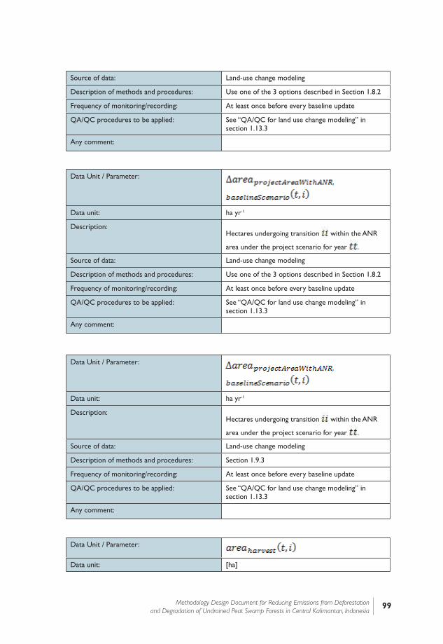
99Methodology Design Document for Reducing Emissions from Deforestation and Degradation of Undrained Peat Swamp Forests in Central Kalimantan, Indonesia
Source of data: Land-use change modeling
Description of methods and procedures: Use one of the 3 options described in Section 1.8.2
Frequency of monitoring/recording: At least once before every baseline update
QA/QC procedures to be applied: See “QA/QC for land use change modeling” in section 1.13.3
Any comment:
Data Unit / Parameter:
Data unit: ha yr-1
Description:Hectares undergoing transition within the ANR
area under the project scenario for year .
Source of data: Land-use change modeling
Description of methods and procedures: Section 1.9.3
Frequency of monitoring/recording: At least once before every baseline update
QA/QC procedures to be applied: See “QA/QC for land use change modeling” in section 1.13.3
Any comment:
Data Unit / Parameter:
Data unit: [ha]

100 Section I: Carbon MRV Methodology
Description:Area of forest land in harvest stratum that is
harvested at time of the crediting period
Source of data: Log of harvesting activities
Description of methods and procedures:
Frequency of monitoring/recording: Every time harvesting occurs
QA/QC procedures to be applied: See “QA/QC for data entry, documentation and analyses” in section 1.13.3
Any comment:
Data Unit / Parameter:
Data unit: [-]
Description: The proportion of biomass removed by harvesting
for harvest stratum and year .
Source of data: Log of harvesting activities
Description of methods and procedures:
Frequency of monitoring/recording: At least once before every verification
QA/QC procedures to be applied: See “QA/QC for data entry, documentation and analyses” in section 1.13.3
Any comment: Values may be constrained by the timber available for commercial harvest.
Data Unit / Parameter:
Data unit: [-]
Description: The proportion of additional biomass removed for road/track and landing construction for harvest
stratum and year .
Source of data: Regional and local comparative studies and experimental information derived from the local forest industry.
Description of methods and procedures:
Frequency of monitoring/recording: At least once before every verification. Previous values remain valid if no more recent values are found in the literature.
QA/QC procedures to be applied:
Any comment:
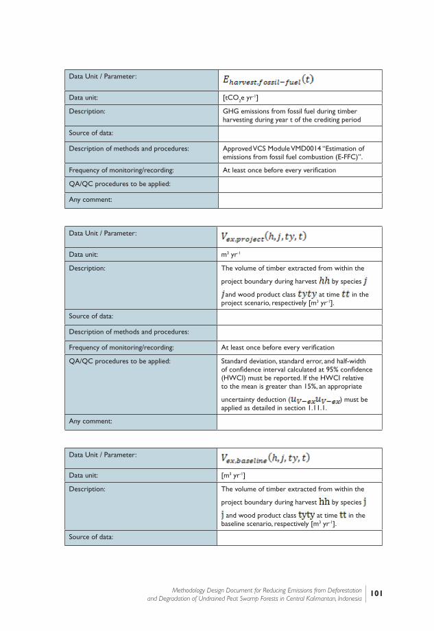
101Methodology Design Document for Reducing Emissions from Deforestation and Degradation of Undrained Peat Swamp Forests in Central Kalimantan, Indonesia
Data Unit / Parameter:
Data unit: [tCO2e yr-1]
Description: GHG emissions from fossil fuel during timber harvesting during year t of the crediting period
Source of data:
Description of methods and procedures: Approved VCS Module VMD0014 “Estimation of emissions from fossil fuel combustion (E-FFC)”.
Frequency of monitoring/recording: At least once before every verification
QA/QC procedures to be applied:
Any comment:
Data Unit / Parameter:
Data unit: m3 yr-1
Description: The volume of timber extracted from within the
project boundary during harvest by species
and wood product class at time in the project scenario, respectively [m3 yr-1].
Source of data:
Description of methods and procedures:
Frequency of monitoring/recording: At least once before every verification
QA/QC procedures to be applied: Standard deviation, standard error, and half-width of confidence interval calculated at 95% confidence (HWCI) must be reported. If the HWCI relative to the mean is greater than 15%, an appropriate
uncertainty deduction ( ) must be applied as detailed in section 1.11.1.
Any comment:
Data Unit / Parameter:
Data unit: [m3 yr-1]
Description: The volume of timber extracted from within the
project boundary during harvest by species
and wood product class at time in the baseline scenario, respectively [m3 yr-1].
Source of data:
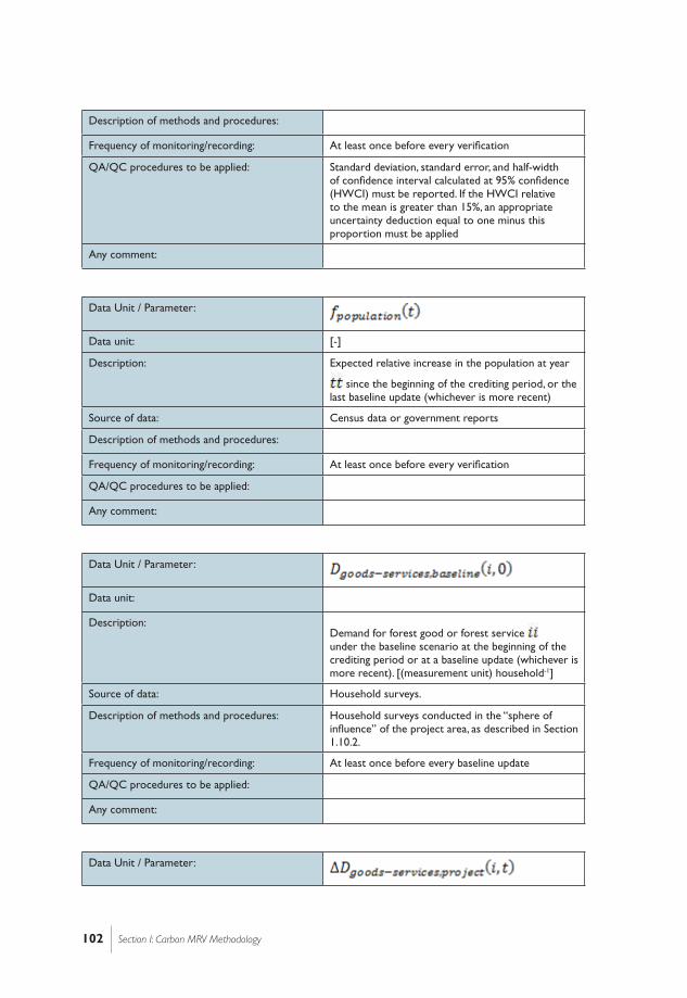
102 Section I: Carbon MRV Methodology
Description of methods and procedures:
Frequency of monitoring/recording: At least once before every verification
QA/QC procedures to be applied: Standard deviation, standard error, and half-width of confidence interval calculated at 95% confidence (HWCI) must be reported. If the HWCI relative to the mean is greater than 15%, an appropriate uncertainty deduction equal to one minus this proportion must be applied
Any comment:
Data Unit / Parameter:
Data unit: [-]
Description: Expected relative increase in the population at year
since the beginning of the crediting period, or the last baseline update (whichever is more recent)
Source of data: Census data or government reports
Description of methods and procedures:
Frequency of monitoring/recording: At least once before every verification
QA/QC procedures to be applied:
Any comment:
Data Unit / Parameter:
Data unit:
Description:Demand for forest good or forest service under the baseline scenario at the beginning of the crediting period or at a baseline update (whichever is more recent). [(measurement unit) household-1]
Source of data: Household surveys.
Description of methods and procedures: Household surveys conducted in the “sphere of influence” of the project area, as described in Section 1.10.2.
Frequency of monitoring/recording: At least once before every baseline update
QA/QC procedures to be applied:
Any comment:
Data Unit / Parameter:

103Methodology Design Document for Reducing Emissions from Deforestation and Degradation of Undrained Peat Swamp Forests in Central Kalimantan, Indonesia
Data unit:
Description: Reduction in demand for forest good or forest
service due to project activities. [(measurement unit)]
Source of data:
Description of methods and procedures: Calculate based on actual records of activity implementation
Frequency of monitoring/recording: At least once before every verification
QA/QC procedures to be applied: See “QA/QC for data entry, documentation and analyses” in section 1.13.3
Any comment:
Data Unit / Parameter:
Data unit: [kg N yr-1]
Description:Mass of synthetic fertilizer type applied in year
. is the difference between the synthetic fertilizer applied during the project in
year and the synthetic fertilizer applied during the baseline. The amount of synthetic fertilizer used per cropping system and per project parcel in the baseline must be quantified and monitored.
Source of data: At least once before every verification
Description of methods and procedures:
Frequency of monitoring/recording:
QA/QC procedures to be applied:
Any comment:
Data Unit / Parameter:
Data unit: [kg N yr-1]
Description:Mass of organic fertilizer type applied in year .
Source of data: Household surveys.
Description of methods and procedures:is the difference between the
organic fertilizer applied during the project in year
and the organic fertilizer applied during the baseline.

104 Section I: Carbon MRV Methodology
Frequency of monitoring/recording: At least once before every verification
QA/QC procedures to be applied:
Any comment:
Data Unit / Parameter:
Data unit: [ha yr-1]
Description: Annual difference in harvested area of rice for the
sub-unit, as defined by conditions , , and , between project and baseline scenario [ha yr-1]. The
area of rice cultivation for each condition , ,
and and for each individual project parcel in the baseline must be quantified using Participatory Rural Appraisals, and re-evaluated regularly.
Source of data: Household surveys
Description of methods and procedures:
Frequency of monitoring/recording: At least once before every verification
QA/QC procedures to be applied:
Any comment:
Data Unit / Parameter:
Data unit: [tCO2e yr-1]
Description: GHG Emissions from Increased Livestock Stocking Rates
Source of data:
Description of methods and procedures: Use the most recent version of approved CDM methodology AR-AM00061, section 8, “Leakage” to determine the CH4 and N2O emissions from livestock, as well as the CDM AR tool “Estimation of GHG emissions related to displacement of grazing activities in A/R CDM project activity”2.
Frequency of monitoring/recording: At least once before every verification
QA/QC procedures to be applied:
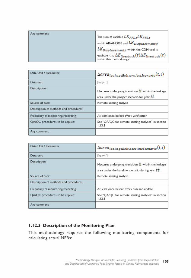
105Methodology Design Document for Reducing Emissions from Deforestation and Degradation of Undrained Peat Swamp Forests in Central Kalimantan, Indonesia
Any comment:The sum of variable
within AR-AM0006 and
within the CDM tool is
equivalent to within this methodology.
Data Unit / Parameter:
Data unit: [ha yr-1]
Description:Hectares undergoing transition within the leakage
area under the project scenario for year .
Source of data: Remote sensing analysis
Description of methods and procedures:
Frequency of monitoring/recording: At least once before every verification
QA/QC procedures to be applied: See “QA/QC for remote sensing analyses” in section 1.13.3
Any comment:
Data Unit / Parameter:
Data unit: [ha yr-1]
Description:Hectares undergoing transition within the leakage
area under the baseline scenario during year .
Source of data: Remote sensing analysis
Description of methods and procedures:
Frequency of monitoring/recording: At least once before every baseline update
QA/QC procedures to be applied: See “QA/QC for remote sensing analyses” in section 1.13.3
Any comment:
1.12.3 Description of the Monitoring Plan
This methodology requires the following monitoring components for calculating actual NERs:
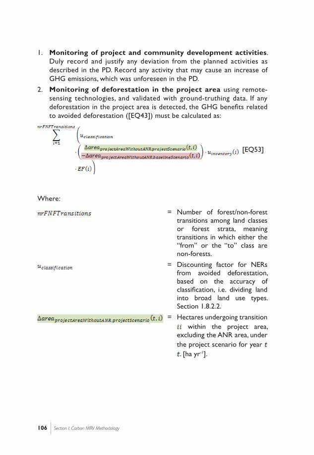
106 Section I: Carbon MRV Methodology
1. Monitoring of project and community development activities. Duly record and justify any deviation from the planned activities as described in the PD. Record any activity that may cause an increase of GHG emissions, which was unforeseen in the PD.
2. Monitoring of deforestation in the project area using remote-sensing technologies, and validated with ground-truthing data. If any deforestation in the project area is detected, the GHG benefits related to avoided deforestation ([EQ43]) must be calculated as:
[EQ53]
Where:
= Number of forest/non-forest transitions among land classes or forest strata, meaning transitions in which either the “from” or the “to” class are non-forests.
= Discounting factor for NERs from avoided deforestation, based on the accuracy of classification, i.e. dividing land into broad land use types. Section 1.8.2.2.
= Hectares undergoing transition within the project area,
excluding the ANR area, under the project scenario for year . [ha yr-1].

107Methodology Design Document for Reducing Emissions from Deforestation and Degradation of Undrained Peat Swamp Forests in Central Kalimantan, Indonesia
= Hectares undergoing transition within the project area,
excluding the ANR area, under the baseline scenario for year . [ha yr-1].
= Discounting factor for all emission reductions, based on the uncertainty of biomass inventory related to transition
.
= Emission Factor for transition .
3. Monitoring carbon stock densities in LULC classes. The emission factors used in [EQ43], [EQ45], [EQ46], and [EQ47] must be calculated using the most recent biomass inventories. The number of sampling plots may be gradually expanded after the project start. Since the number of plots included in the emission factor calculation at verification may be
different from the number of plots included at validation,
, must be re-calculated with the most recent number of sampling plots at verification. However, no biomass inventories older than five years before a verification event may be used for calculating the emission factors.
4. Monitoring carbon in long-lived wood products. Ex-post,
must be monitored and quantified using forest operation records (i.e., log books kept as part of forest management plan). The uncertainty around the monitored volume of timber must be explicitly reported. Ex-post baseline
must be estimated from literatures and if such data is not available, then it must be set equal to the existing demand for volume of wood products including leakage but excluding community development activities.
5. Monitoring carbon stock increases in the area on which ANR are performed.
6. Monitoring of natural disturbances, if any occurred during the last verification period.

108 Section I: Carbon MRV Methodology
7. Monitoring of leakage from displaced forest conversion. Project proponents must estimate the size of the annual area that has been sanctioned for the same conversion scenario(s) as the ones identified under the baseline scenario of the project by the relevant administrative jurisdiction that governs over the province, state, or country in which the project area is located. A one-sided t-test must be executed to determine whether the actual area allotted for land conversion is greater than 15% of the average amount of area allotted for the specific
conversion with 95% confidence. If it is greater,
in Equation [EQ48] must be set to the difference in area between the actual area for land conversion and the average area predicted based on the data used in the t-test.
8. Monitoring of displaced extraction of forest goods and services. Social assessments must be conducted among the communities that were using the project area to extract goods and services before the start of the project. Using the social assessments, the project proponents must determine (1) the extraction rates and locations of forest goods and services after the start of the crediting period, and (2) how project actions and community development activities may have decreased the extraction rates and locations of forest goods and services. The monitoring procedure of the impact of leakage from displaced extraction of forest goods and services is dependent on whether the extraction of forest goods and services likely leads to deforestation (see Section 1.8.5.3).a. For goods and services that likely lead to deforestation, leakage must
be calculated by monitoring increases in the deforestation rate in leakage belts compared to historically observed deforestation rate
[EQ54]
Where:
= GHG emissions from leakage related to the extraction of forest goods and services that likely lead to deforestation during year of the crediting period [tCO2e]
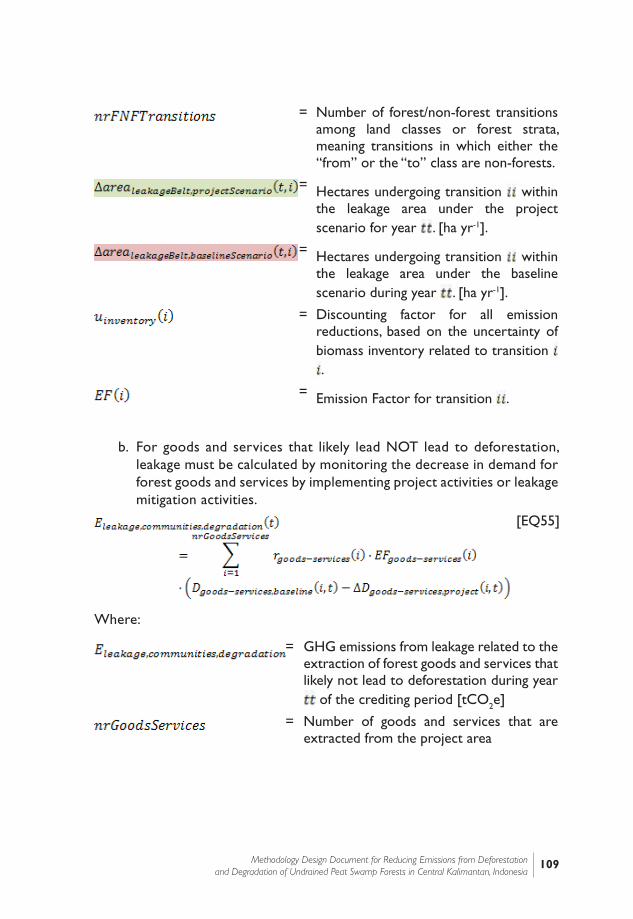
109Methodology Design Document for Reducing Emissions from Deforestation and Degradation of Undrained Peat Swamp Forests in Central Kalimantan, Indonesia
= Number of forest/non-forest transitions among land classes or forest strata, meaning transitions in which either the “from” or the “to” class are non-forests.
= Hectares undergoing transition within the leakage area under the project scenario for year . [ha yr-1].
= Hectares undergoing transition within the leakage area under the baseline scenario during year . [ha yr-1].
= Discounting factor for all emission reductions, based on the uncertainty of biomass inventory related to transition .
= Emission Factor for transition .
b. For goods and services that likely lead NOT lead to deforestation, leakage must be calculated by monitoring the decrease in demand for forest goods and services by implementing project activities or leakage mitigation activities.
[EQ55]
Where:
= GHG emissions from leakage related to the extraction of forest goods and services that likely not lead to deforestation during year
of the crediting period [tCO2e]
= Number of goods and services that are extracted from the project area
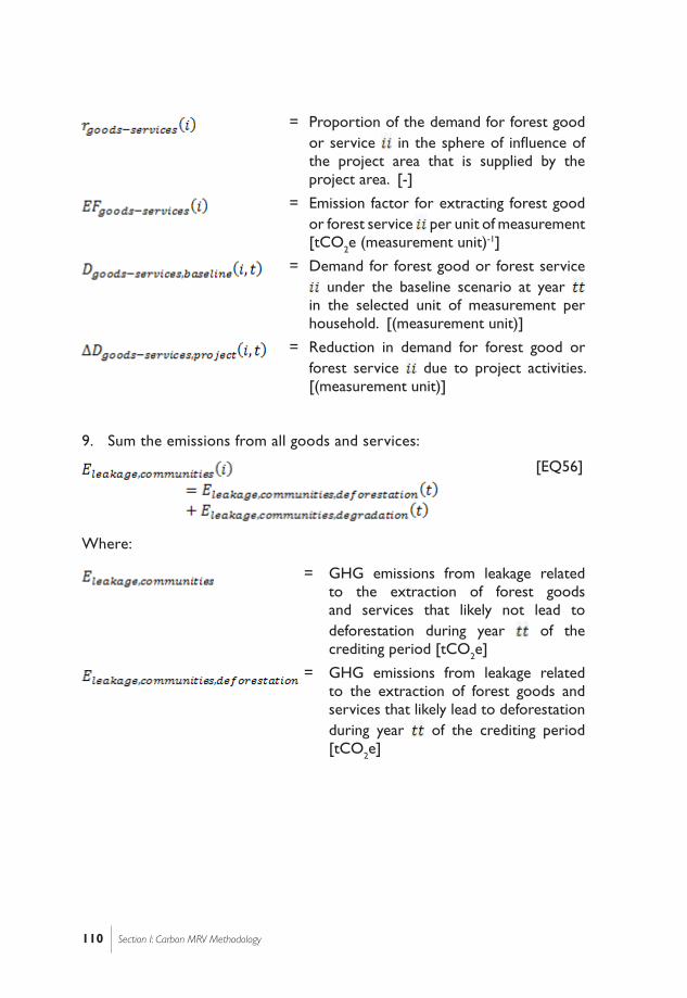
110 Section I: Carbon MRV Methodology
= Proportion of the demand for forest good or service in the sphere of influence of the project area that is supplied by the project area. [-]
= Emission factor for extracting forest good or forest service per unit of measurement [tCO2e (measurement unit)-1]
= Demand for forest good or forest service under the baseline scenario at year
in the selected unit of measurement per household. [(measurement unit)]
= Reduction in demand for forest good or forest service due to project activities. [(measurement unit)]
9. Sum the emissions from all goods and services:
[EQ56]
Where:
= GHG emissions from leakage related to the extraction of forest goods and services that likely not lead to deforestation during year of the crediting period [tCO2e]
= GHG emissions from leakage related to the extraction of forest goods and services that likely lead to deforestation during year of the crediting period [tCO2e]
111Methodology Design Document for Reducing Emissions from Deforestation and Degradation of Undrained Peat Swamp Forests in Central Kalimantan, Indonesia
= GHG emissions from leakage related to the extraction of forest goods and services that likely not lead to deforestation during year of the crediting period [tCO2e]
A monitoring report is produced which contains all of the information above, and which outlines the calculations for actual NERs generated. This monitoring report is the basis for verification by VCS-accredited verifiers. The actual VCUs are released upon verification and positive evaluation of a monitoring. The VCS requires that verification takes place minimally every five years. Project proponents may choose to seek verification more frequently, especially in the beginning of the crediting period. The PD must contain a fixed time schedule of when verification will be sought during the full duration of the crediting period.
At every verification time, project proponents must check that no other land-based carbon projects registered under the CDM or under any other carbon trading scheme (both voluntary and compliance-oriented) are present in the project area. A formal statement on the lack of any other carbon project in the project area must be included in the monitoring report.
Monitoring plan description requirements in PD
Include the following elements in the monitoring plan:
1. Variables to be tracked continuously
a. Authority responsible for tracking.b. List of variables that will be tracked continuously.c. Which potential natural disturbances are foreseen?d. Who will record information on natural disturbances?e. How will adoption rates and super-acceptance leakage be monitored?

112 Section I: Carbon MRV Methodology
2. Variables to be monitored periodically
a. Decision on monitoring frequency and rationale.b. Decision on the duration of the subsequent monitoring period.c. Who will monitor the boundaries of the project regions?d. Field inventory§Sample size rationale
§Sampling plot size and layout rationale
§Sampling plot location
§Standard Operations Procedure for field sampling.
e. Information on agents and drivers§List of variables to be collected.§If a social appraisal needs to be conducted, a list of the variables to be
queried.
3. Decision and rationale on the period of baseline validation.
4. All relevant information on natural disturbances & catastrophes.
1.13 OtherInformation
1.13.1 Guidance on Social Assessments
Social assessments must be conducted to collect social information regarding project conditions. For most data items that are to be collected within the methodology, personal interviews with individual households are preferred; these are referred to as “household surveys”. However, for data items that are more challenging to quantify such as forest fires and forest encroachment, semi-structured focus group discussions with representative community members are more appropriate; these are referred to as “participatory rural appraisals”. The sample size for household surveys can be based on a comparatively small proportion of the target population (UN 2008). The required number of household surveys must be selected so that a minimal confidence level of 95% is attained. The exact number of surveys can be determined using the formula in Krejcie and Morgan (1970). In case of semi-structured interviews in participatory rural appraisals; at least 10 focus group discussions must be conducted. Further guidelines for carrying out these appraisals can be found in
113Methodology Design Document for Reducing Emissions from Deforestation and Degradation of Undrained Peat Swamp Forests in Central Kalimantan, Indonesia
Cochran (1977), Freudenberger (1994), Kish (1995), Top et al. (2004) and UN (2008). The following steps are to be followed for designing and conducting surveys.
1. Assemble all information that must be collected and determine the goals of the questionnaire. Identify all information that is required by the methodology.
2. Determine the target group of the questionnaire, and sub-divide the group into different strata. Strata must be defined according to one or more of the combination of geography, household size, age, gender, etc. Take proper care to avoid the selection of a biased target group.
3. Determine the total sample size and the number of samples required in each stratum. Identify the population in each of the strata categories defined in the previous step. Set quotas, a minimal number of surveys from each of the sample strata. Surveys must be collected until the quotas have been reached.
4. Create your questionnaire. Transformthe required data into neutral, simple and systematic questions. If possible and relevant, generate a set of expected answers. Include partially redundant questions to ensure consistency of data. Include space for some sketch mapping, if relevant. Expected answers could be complemented with graphs, figures, maps and pictures. Allow a “not applicable” or “uncertain” category. Group questions logically according to their contents and leave difficult or sensitive questions until near the end of a survey.
5. Choose interviewing methodology and develop a standard operations procedure for interviewing. Include QA/QC procedures such as re-sampling a randomly selected sub-group by different experts, and the requirement to take geo-tagged pictures. All surveys must contain date, time, location, and name of the expert who conducted the survey. In addition, include a section on how to introduce the purpose of the questionnaires to the interviewees.
6. Pre-test the questionnaire and methodology, and adjust the questionnaire and its methodology, if necessary. More specifically, if questions are multiple choice (discrete), ensure that all potential answers are included.
7. Train experts for conducting interviews. Through instruction, role playing exercises, and test sessions followed by immediate feedback, train experts to conduct interviews. These experts are properly trained in explaining the broader scope of the social assessments.
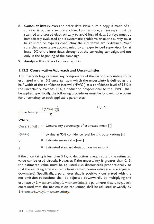
114 Section I: Carbon MRV Methodology
8. Conduct interviews and enter data. Make sure a copy is made of all surveys is put in a secure archive. Furthermore, all surveys must be scanned and stored electronically to avoid loss of data. Surveys must be immediately evaluated and if systematic problems arise, the survey must be adjusted or experts conducting the interviews are re-trained. Make sure that experts are accompanied by an experienced supervisor for at least 10% of the interviews throughout the surveying campaign, and not only in the beginning of the campaign.
9. Analyze the data - Produce reports.
1.13.2 Conservative Approach and Uncertainties
This methodology requires key components of the carbon accounting to be estimated within 15% uncertainty, in which the uncertainty is defined as the half-width of the confidence interval (HWCI) at a confidence level of 95%. If the uncertainty exceeds 15%, a deduction proportional to the HWCI shall be applied. Specifically, the following procedures must be followed to account for uncertainty to each applicable parameter.
[EQ57]
Where,
= Uncertainty percentage of estimated mean [-]
= t-value at 95% confidence level for observations [-]
= Estimate mean value [unit]
= Estimated standard deviation on mean [unit]
If the uncertainty is less than 0.15, no deduction is required and the estimated value can be used directly. However, if the uncertainty is greater than 0.15, the estimated value must be adjusted (i.e. discounted) proportionally so that the resulting emission reductions remain conservative (i.e., are adjusted downward). Specifically, a parameter that is positively correlated with the net emission reductions shall be adjusted downwardly by multiplying the estimate by ; a parameter that is negatively correlated with the net emission reductions shall be adjusted upwardly by
.

115Methodology Design Document for Reducing Emissions from Deforestation and Degradation of Undrained Peat Swamp Forests in Central Kalimantan, Indonesia
1.13.2.1 Uncertainty of Key Components of Methodology
The following is a list of the key components of the carbon accounting for which the uncertainty must be estimated and reported, and for which uncertainty deductions must be applied:
1. For baseline deforestation rates using remote sensing classification,
, factors are selected based on the empirically observed accuracy of discerning forest/non-forest classes, and forest biomass classes, respectively, according to the procedures outlined in this methodology.
2. Emission factors from tree biomass must be discounted with
, which equals the half-width of the confidence interval of the mean difference between the two carbon stock densities. Note that the minimum desired level of precision for sampling design of biomass inventory is 15%.
3. Biomass stock densities calculated using allometric equations shall be discounted if the allometric equation is not accurate within 15% (see Section C13).
4. ANR growth rates shall be discounted downwardly using the half-width of the confidence interval.
5. Subsidence rates shall be discounted downwardly using the half-width of the confidence interval
6. For peat depth, the uncertainty deduction is applied indirectly, by limiting the total size of the peat area to the area for which the confidence that the required minimal peat depth is met is at least 95%. Uncertainty deductions can be avoided by increasing the sampling size of peat depth measurements.
1.13.3 Quality Assurance and Quality Control Procedures
To ensure the precise, verifiable and transparent calculation of net NERs, a quality assurance and quality control (QA/QC) procedure shall be implemented.
1.13.3.1 QA/QC for field measurements
1. Persons involved in the field measurement work are trained in the field data collection and data analyses.
116 Section I: Carbon MRV Methodology
2. List all names of the field teams and the project leader and the dates of the training sessions.
3. Record which teams have measured each sampling plot. Record who was responsible for each task.
4. Develop Standard Operating Procedures (SOPs) for each step of the field measurements and adhere to these at all times, both ex-ante and ex-post.
5. Put a mechanism in place to correct potential errors or inadequacies in the SOPs by a qualified person.
6. Verify that plots have been installed and measured correctly, by having approximately 10% of all plots re-measured by an independent team. If the deviation between measurement and re-measurement is larger than 5%, investigate the source of the error, record and correct.
1.13.3.2 QA/QC for data entry, documentation and analyses
1. Review the entry of data into the data analyses spreadsheets by an independent source.
2. Archived all original data sheets safely. Electronic data shall be backed up adequately on durable media.
3. Ensure that all files are named appropriately. Ensure that all database fields, spreadsheet headings or cells are adequately documented in such a way that it can be verified independently.
4. Verify calculations for trivial errors such as unit conversion errors.
5. If parameters are common between analyses (e.g., emission factors), ensure that consistent values are used.
6. Check for consistency among time series data. Identify outliers as soon after the actual measurement as possible. Investigate the cause of the outlying observation, and correct if needed.
7. Compare estimates from field measurements or social appraisals with literature values.
8. An SOP for non-biomass monitoring must be developed and adhered to at all times.
1.13.3.3 QA/QC for remote sensing analyses
1. Develop Standard Operating Procedures (SOPs) for each step of the remote sensing analyses and adhere to these at all times, both ex-ante and ex-post.
117Methodology Design Document for Reducing Emissions from Deforestation and Degradation of Undrained Peat Swamp Forests in Central Kalimantan, Indonesia
2. Use ground-truthing data to validate the LULC classification and forest stratification. Use confusion matrices and accuracy indices to analyze and quantify the accuracy of the classification.
3. Use visual interpretation of high-resolution satellite imagery to complement the medium resolution imagery.
4. Check for consistency among time series data. If outliers are present (e.g., in deforestation quantities), analyze the cause and correct if errors were made.
5. Compare estimates of deforestation and forest degradation rates with relevant estimates from the literature.
1.13.3.4 QA/QC for land use change modeling
1. Split the available data in 2/3 for calibration purposes, and 1/3 for validation purposes. Never use the same data for calibration and validation.
2. Report a measure for the accuracy of the land use change model.
1.14 Verification Procedure of Allometric Equations
Every time one or more new equations are proposed, the proposed equation(s) must be verified according to the following criteria:
1. The proposed equation(s) must have an r2 value of greater than 0.5 (50%) and a p-value that is significant at 95% confidence level as reported in the source publications.
2. The proposed equation(s) was developed from trees where the largest and smallest DBH of the trees fall within the DBH range of the trees within the project areas.
3. If the proposed equation(s) was/were derived from data solely from within the reference region then such equations can be used. If the proposed equation(s) was/were derived outside of the reference region, project proponents must justify the similarity in climatic, edaphic, geographical and species composition between the project area and the location from where the equations were derived. The source publication must include an estimate of the uncertainty or sufficient data to estimate the uncertainty. If this uncertainty is within ±15% of the mean values and is not biased in a non-conservative manner (i.e., the equation(s) do(es) not systematically overestimate the project net anthropogenic removals by sinks), the equation(s) may be used.

118 Section I: Carbon MRV Methodology
4. For any other equations that do not satisfy criteria (d) or if new equations or equations which do not have estimate of uncertainty are to be used, then one of the following two approaches must be carried out:a. Destructive Sampling
• Selecting at least 5 trees covering the range of DBH existing in the project area, and felling and weighing the above-ground biomass to determine the total (green) weight of the stem an branch components
• Extracting and immediately weighing subsamples from each of the green stems and branch component, followed by oven drying at 70°C to determine dry biomass.
• Determine the total dry weight of each tree from the green weights and the averaged ratios of wet and dry weights of the stem and branch components.
b. Limited Measurements• Select at least 10 trees per species distributed across the project
area
• Calculate volume of tree from basal and top diameters and tree height. Multiply by species-specific density to gain biomass of bole. Add an additional 20 percentage of weight to approximately cover the biomass of branches.
If the biomass of the measured trees is within ±15% of the mean values predicted by the selected default allometric equation, and is not biased – or if biased towards the conservative side (i.e., equation underestimates of the project net anthropogenic removals by sinks), then mean values from the equation may be used. However, if the If the biomass of the measured trees is not within ±15% of the mean values predicted by the selected default allometric equation, estimated biomass must be further discounted with the relative average half-width of the confidence interval of the model.

119Methodology Design Document for Reducing Emissions from Deforestation and Degradation of Undrained Peat Swamp Forests in Central Kalimantan, Indonesia
Section 2: Social Safeguards
In order to protect the rights and interests of indigenous peoples and forest-dependent communities in REDD+, social safeguards were included in the Cancun Agreements. It is important that they address not only “no harm” to indigenous peoples and local communities, but also promote governance and multiple social benefits.
The following Box 1 highlights key checkpoints in designing a social safeguards methodology. This section further explores social safeguards by using a case study from the Katingan Project.
Box 1. Social Safeguards Methodology Design Checkpoints• Conduct a participatory rural appraisal • The assignment of community development facilitators• Stakeholder analysis and social mapping• Livelihood analysis• Participatory land-use mapping
• Conduct FPIC with community members• Provision of open and balanced information on REDD+ activities• Recruitment of FPIC facilitators and provision of training to them• Facilitation of FPIC-based negotiation processes• Documentation of FPIC outcomes
• Develop information, education and communication (IEC) mechanisms• Target audience analysis based on stakeholder/social mapping• Development of short-, mid-, and long-term IEC plans and appropriate media• Media broadcast to enhance the understanding, transparency and support of REDD+
activities• Identify and develop market and economic opportunities• Community-level economic feasibility study• Development of appropriate microfinance facilities and microenterprises based on
communities’ needs and desires• Develop benefits and role distribution structures • Identification of rights and responsibilities of communities in implementing REDD+
activities• Development of benefits distribution structures • Periodic monitoring and evaluation
• Implement community capacity building programs• Provision of information and know-how regarding communities’ rights, government laws
and regulations, negotiation skills, and business administration and marketing skills• Build local health and education facilities• Identification of communities’ needs and desires• Improvement or development of clinics, nursery and health education programs, and
schools• Conduct socio-economic impact monitoring and evaluation• Development of monitoring and evaluation criteria• Documentation of positive and/or negative changes in socio-economic wellbeing

120 Section 2:Social Safeguards
2.1 Stakeholder analysis
A stakeholder analysis was conducted based on focus group discussions (FGD) conducted at 4 villages – Terantang, Terantang Hilir, Hanaut and Bapinang Hulu, as well as the results from the pre-FS social surveys. Table 8 presents a list of main stakeholders to be consulted and involved for the implementation of the Katingan Project.
Table 8. List of Stakeholders and their role function in the REDD+ Implementation in Central Kalimantan
No. Stakeholders Roles and Contribution of Stakeholders in REDD+ Imple-mentation
Roles Function Power Influ-ence
1. Government of Central Kalimantan Province
Providing local regu-lations on REDD+ implementation at the district level
Facilitator and advisor for REDD+ implementation
+ +
2. Government of East Kota War-ingin District
Providing local regu-lations on REDD+ implementation at the sub-district level
Facilitator and advisor for REDD+ implementation
++ +
3. Government of Katingan District
Providing local regu-lations on REDD+ implementation at the sub-district level
Facilitator and advisor for REDD+ implementation
++ +
4. Heads of Sub-districts in East Kotawaringin District
Coordinating and supervising REDD+ implementation at the village level
Coordinator and su-pervisor for REDD+ implementation
+ ++
5. Heads of Vil-lages in the sub-districts of East Kotawaringin District
Providing approv-als for REDD+ field implementation in the village area
Key person for a smooth REDD+ implementation
+++ ++
6. Heads of Sub-districts in Kat-ingan District
Coordinating and supervising REDD+ implementation at the village level
Coordinator and su-pervisor for REDD+ implementation
+ ++

121Methodology Design Document for Reducing Emissions from Deforestation and Degradation of Undrained Peat Swamp Forests in Central Kalimantan, Indonesia
No. Stakeholders Roles and Contribution of Stakeholders in REDD+ Imple-mentation
Roles Function Power Influ-ence
7. Heads of Vil-lages in the sub-districts of Katingan District
Providing approv-als for REDD+ field implementation in the village area
Key person for a smooth REDD+ implementation
+++ ++
8. Heads of com-munity and farmer groups at the village level
Providing advice and guidance for issues and opportunities faced by communi-ties
Advisor and leader at the community level
+++ +++
9. Non Govern-mental Organi-zations
Facilitating and build-ing capacity for local community members
Facilitator and trainer for REDD+ implementation
+ +++
2.2 Drivers and agents of deforestation and mitigation measures
2.2.1 Drivers and agents of deforestation
Indonesia’s forests are disappearing at an alarming rate. A study estimated that over 30% of Indonesia’s peat-swamp forest became degraded from 1985-2005, and average degradation rates continue at a rate of 1.7% a year (Hooijer et al., 2006). The peat swamp forest of the Katingan Project area is no exception.
It is important that both direct and indirect drivers of deforestation are addressed in implementing the Katingan Project. Direct drivers and agents of deforestation in and around the project area are presented in Table 9.
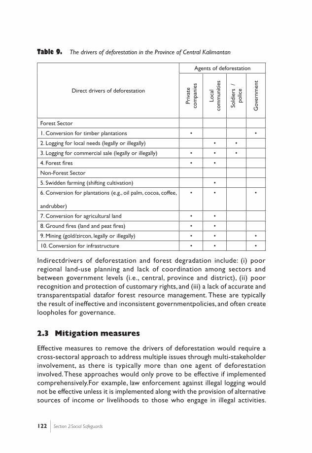
122 Section 2:Social Safeguards
Table 9. The drivers of deforestation in the Province of Central Kalimantan
Direct drivers of deforestation
Agents of deforestation
Priv
ate
com
pani
es
Loca
l co
mm
uniti
es
Sold
iers
/
polic
e
Gov
ernm
ent
Forest Sector
1. Conversion for timber plantations • •
2. Logging for local needs (legally or illegally) • •
3. Logging for commercial sale (legally or illegally) • • •
4. Forest fires • •
Non-Forest Sector
5. Swidden farming (shifting cultivation) •
6. Conversion for plantations (e.g., oil palm, cocoa, coffee,
andrubber)
• • •
7. Conversion for agricultural land • •
8. Ground fires (land and peat fires) • •
9. Mining (gold/zircon, legally or illegally) • • •
10. Conversion for infrastructure • • •
Indirectdrivers of deforestation and forest degradation include: (i) poor regional land-use planning and lack of coordination among sectors and between government levels (i.e., central, province and district), (ii) poor recognition and protection of customary rights, and (iii) a lack of accurate and transparentspatial datafor forest resource management. These are typically the result of ineffective and inconsistent governmentpolicies, and often create loopholes for governance.
2.3 Mitigation measures
Effective measures to remove the drivers of deforestation would require a cross-sectoral approach to address multiple issues through multi-stakeholder involvement, as there is typically more than one agent of deforestation involved. These approaches would only prove to be effective if implemented comprehensively.For example, law enforcement against illegal logging would not be effective unless it is implemented along with the provision of alternative sources of income or livelihoods to those who engage in illegal activities.
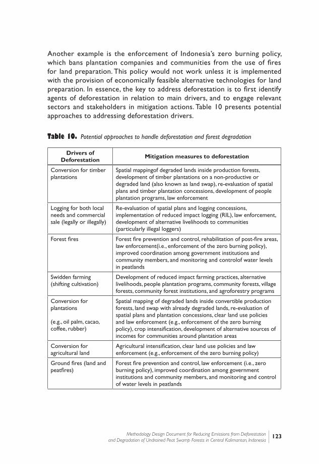
123Methodology Design Document for Reducing Emissions from Deforestation and Degradation of Undrained Peat Swamp Forests in Central Kalimantan, Indonesia
Another example is the enforcement of Indonesia’s zero burning policy, which bans plantation companies and communities from the use of fires for land preparation. This policy would not work unless it is implemented with the provision of economically feasible alternative technologies for land preparation. In essence, the key to address deforestation is to first identify agents of deforestation in relation to main drivers, and to engage relevant sectors and stakeholders in mitigation actions. Table 10 presents potential approaches to addressing deforestation drivers.
Table 10. Potential approaches to handle deforestation and forest degradation
Drivers of Deforestation Mitigation measures to deforestation
Conversion for timber plantations
Spatial mappingof degraded lands inside production forests, development of timber plantations on a non-productive or degraded land (also known as land swap), re-evaluation of spatial plans and timber plantation concessions, development of people plantation programs, law enforcement
Logging for both local needs and commercial sale (legally or illegally)
Re-evaluation of spatial plans and logging concessions, implementation of reduced impact logging (RIL), law enforcement, development of alternative livelihoods to communities (particularly illegal loggers)
Forest fires Forest fire prevention and control, rehabilitation of post-fire areas, law enforcement(i.e., enforcement of the zero burning policy), improved coordination among government institutions and community members, and monitoring and controlof water levels in peatlands
Swidden farming (shifting cultivation)
Development of reduced impact farming practices, alternative livelihoods, people plantation programs, community forests, village forests, community forest institutions, and agroforestry programs
Conversion for plantations
(e.g., oil palm, cacao, coffee, rubber)
Spatial mapping of degraded lands inside convertible production forests, land swap with already degraded lands, re-evaluation of spatial plans and plantation concessions, clear land use policies and law enforcement (e.g., enforcement of the zero burning policy), crop intensification, development of alternative sources of incomes for communities around plantation areas
Conversion for agricultural land
Agricultural intensification, clear land use policies and law enforcement (e.g., enforcement of the zero burning policy)
Ground fires (land and peatfires)
Forest fire prevention and control, law enforcement (i.e., zero burning policy), improved coordination among government institutions and community members, and monitoring and control of water levels in peatlands

124 Section 2:Social Safeguards
Drivers of Deforestation Mitigation measures to deforestation
Mining (gold / zircon, legally or illegally)
Forest and land rehabilitation, reduction of open-pit mining operations, law enforcement, development of alternative sources of incomes for communities around mining areas, re-evaluation of mining concessions in forest areas
Conversion for infrastructure
Re-evaluation of spatial plans, clear land use policies and law enforcement
2.4 Information, Education and Communication (IEC) Methodology
Information, education and communication (IEC) is a comprehensive communication strategy, which combines different approaches and methods for each target audience such as individuals, families, groups, organizations and communities. Embodied in IEC is the process of learning that empowers people to make decisions, modify behaviors and change social conditions. Thus, an effective IEC methodology should be developed based on different needs, socio-economic conditions and the capacity of local communities as well as local governments, NGOs and other stakeholders.
The IEC strategy comprises of four steps, namely: (i) planning, (ii) implementation, (iii) monitoring and (iv) evaluation. Developing each step should involve, at minimum, local governments, heads of villages and farmer groups, local NGOs, local media, businesses and key industries,educators, local communities and youth groups as key stakeholders for a successful IEC implementation. Table 11 shows the IEC strategy and expected outputs.
Table 11. Information, Education and Communication strategy and expected outputs.
IEC method Description Outputs
Target audience analysis based on stakeholder mapping
Identify representatives of each stakeholder group to reach wide audiences, and determine appropriate IEC methods and communication strategies reflecting local tradition and customs
Target audience identified and IEC methods and communication strategies selected
Producing media Develop short-, mid-, and long-term IEC plan and appropriate media based on the availability of resources and financial capacity
Short-term IEC plan
Mid-term IEC plan
Long-term IEC plan

125Methodology Design Document for Reducing Emissions from Deforestation and Degradation of Undrained Peat Swamp Forests in Central Kalimantan, Indonesia
IEC method Description Outputs
Media broadcast Produce and disseminate materials to local, national, and international audiences in order to enhance the understanding, transparency and support of REDD+ activities
Community radio broadcast
School curriculum and projects
Newsletters produced
Annual gathering and festivals
Monitoring of IEC programs
Develop monitoring guidelines which specify objectives, methods and frequency, and document monitoring results
Monitoring reports
Evaluation of IEC programs
Develop criteria used to assess the progress and effectiveness of IEC programs, and document lessons learned
Evaluation reports which document lessons learned
It is important that media materials are produced and broadcasted in a traditional manner so that local communities can easily be familiarized with the contents. Listed outputs are some of the most common means to disseminate information to public in the Katingan Project area.
2.5 Implementation of Free, Prior and Informed Consent (FPIC) processes
Free, prior and informed consent (FPIC) refers to the rights of local and indigenous peoples to know about and have open access tobalanced information on potential development projects or other activities carried out on their lands. This is to ensure that local people can consider potential impacts of projects critically and negotiate with project developers and other stakeholders based on mutual consensus without being forced or manipulated. Such a consent-based negotiation approach should safeguard legal and customary rights as well as the fundamental importance of local communities associated with lands, territories and natural resources.
In order to establish a basis on which informed, non-coercive agreements between local communities and project developers (and other stakeholders including the government) can be developed, there are fundamental questions to be addressed (Colchester, 2010). They include:
1. Who has the right to FPIC?
2. FPIC over what?
3. Who gives consent?
4. How is consent determined?
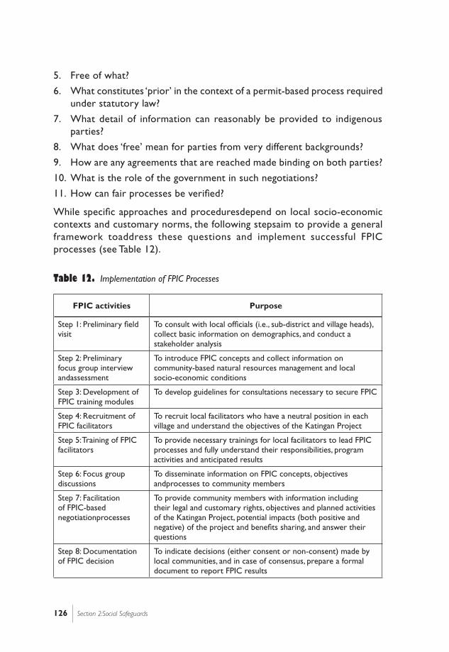
126 Section 2:Social Safeguards
5. Free of what?
6. What constitutes ‘prior’ in the context of a permit-based process required under statutory law?
7. What detail of information can reasonably be provided to indigenous parties?
8. What does ‘free’ mean for parties from very different backgrounds?
9. How are any agreements that are reached made binding on both parties?
10. What is the role of the government in such negotiations?
11. How can fair processes be verified?
While specific approaches and proceduresdepend on local socio-economic contexts and customary norms, the following stepsaim to provide a general framework toaddress these questions and implement successful FPIC processes (see Table 12).
Table 12. Implementation of FPIC Processes
FPIC activities Purpose
Step 1: Preliminary field visit
To consult with local officials (i.e., sub-district and village heads), collect basic information on demographics, and conduct a stakeholder analysis
Step 2: Preliminary focus group interview andassessment
To introduce FPIC concepts and collect information on community-based natural resources management and local socio-economic conditions
Step 3: Development of FPIC training modules
To develop guidelines for consultations necessary to secure FPIC
Step 4: Recruitment of FPIC facilitators
To recruit local facilitators who have a neutral position in each village and understand the objectives of the Katingan Project
Step 5: Training of FPIC facilitators
To provide necessary trainings for local facilitators to lead FPIC processes and fully understand their responsibilities, program activities and anticipated results
Step 6: Focus group discussions
To disseminate information on FPIC concepts, objectives andprocesses to community members
Step 7: Facilitation of FPIC-based negotiationprocesses
To provide community members with information including their legal and customary rights, objectives and planned activities of the Katingan Project, potential impacts (both positive and negative) of the project and benefits sharing, and answer their questions
Step 8: Documentation of FPIC decision
To indicate decisions (either consent or non-consent) made by local communities, and in case of consensus, prepare a formal document to report FPIC results

127Methodology Design Document for Reducing Emissions from Deforestation and Degradation of Undrained Peat Swamp Forests in Central Kalimantan, Indonesia
FPIC activities Purpose
Step 9: Evaluation and verification
To evaluate and verify the FPIC processes by an independent third-party auditor
2.6 Resource-use and livelihoods patterns
2.6.1 Social baseline information
Central Kalimantan has a population of just over 2.2 million according to the 2010 Census. The population grew 2.7% annually between 1990 and 2000, one of the highest provincial growth rates in Indonesia during that time; in the subsequent decade to 2010 the average annual growth rate was slightly over 2.0% (see Table 13).
Table 13. The growth of population in Central Kalimantan
Population (Year)
1971 1980 1990 1995 2000 2010
701,936 1,396,486 1,627,453 954,353 1,857,000 2,212,089
Based on the Central Kalimantan Official Statistics, No 08/11/62/ThV, 7 November 2011, the agricultural, plantation, forestry and fishery sectors accommodates approximately 54.75% of the total labor force in the province. The number indicates that these are key sectors for the local economy. The figures can be seen in the following table 14.
Table 14. Key Sector and number of workers
No. Key Sector Number of workers Percentage
1 Agriculture, Plantation, Forestry, Fishery 605378 54.75
2 Industry 31277 2.83
3 Trade, Restaurant and accommodation services
157741 14.27
4 social community and personal service 151241 13.67
5 Other 160064 14.48
Total 1105701 100

128 Section 2:Social Safeguards
The Katingan Project area encompasses total 24 villages settled alongside Mentaya River in Kotawaringin Timur district and Katingan River in Katingan district.The total population is estimated to be around 40,000 people, with an indication of population growth in some villages, according to the districts’ village monograph of 2009. Seeking economic opportunities, many people transmigrated to this area from the 1980s until mid 2000s. As a result, while the dominant ethnicity is of Dayak descent, communities surrounding the project area are comprised of diverse ethnic origins, including Banjar, Javanese, and Madurese with the majority of Muslim communities. The average income of a household in the area generally ranges from IDR 500.000 to IDR 1,000.000 (USD 55.00 to USD 110.00) per month, and many community members rely on more than a single source of income to diversify economic risks and secure livelihoods.
2.6.2 Resource-use patterns
Most community members around the Katingan Project have traditionally been practicing shifting cultivation as well as small-scale farming. Local traditions and customs (adat) still form a large part of social norms among communities, by which resource-use patterns have been shaped. Traditional farming has been practiced in harmony with the surrounding environment without the use of destructive methods. However, such harmonious ways of living by local communities are quickly transforming because of increasing pressure on resources due to population growth and poverty.
Since 2002, the number of districts in the Central Kalimantan province has increased from 6 to 14 districts. Thishas led to growing pressure on natural resources as new districts required considerable infrastructural development (e.g., human settlements and roads) and industrial expansion (e.g., oil palm plantations and mining operations) to accommodate increasing population and secure district revenues. As industries developed, more people began to seek employment at oil palm plantations and mining companies in search of better economic opportunities. As industrial agriculture often prefers the most cost-effective practices, for example, the use of fire to clear forest lands and the application of large amount of fertilizers and herbicides, land degradation and water pollution are becoming pressing concerns in some villages.
2.6.3 Livelihood patterns
The majority of community members in all studied villages are farmers, and manage and cultivate lands among small farmer groups. As an addition or main source of income, some people run small businesses such as kiosk,
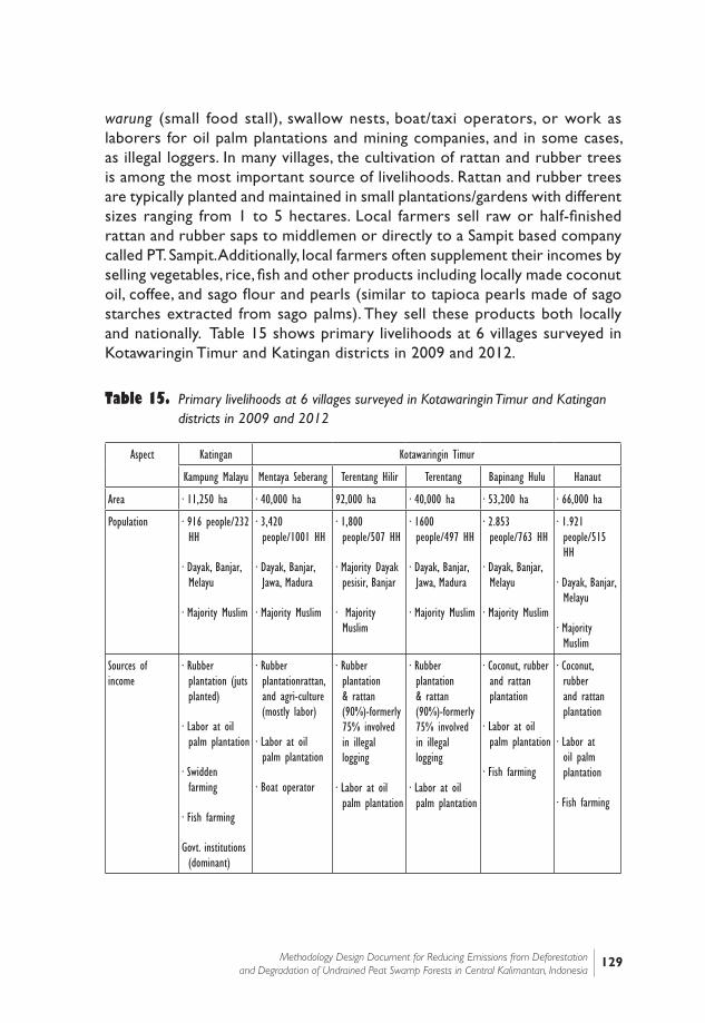
129Methodology Design Document for Reducing Emissions from Deforestation and Degradation of Undrained Peat Swamp Forests in Central Kalimantan, Indonesia
warung (small food stall), swallow nests, boat/taxi operators, or work as laborers for oil palm plantations and mining companies, and in some cases, as illegal loggers. In many villages, the cultivation of rattan and rubber trees is among the most important source of livelihoods. Rattan and rubber trees are typically planted and maintained in small plantations/gardens with different sizes ranging from 1 to 5 hectares. Local farmers sell raw or half-finished rattan and rubber saps to middlemen or directly to a Sampit based company called PT. Sampit. Additionally, local farmers often supplement their incomes by selling vegetables, rice, fish and other products including locally made coconut oil, coffee, and sago flour and pearls (similar to tapioca pearls made of sago starches extracted from sago palms). They sell these products both locally and nationally. Table 15 shows primary livelihoods at 6 villages surveyed in Kotawaringin Timur and Katingan districts in 2009 and 2012.
Table 15. Primary livelihoods at 6 villages surveyed in Kotawaringin Timur and Katingan districts in 2009 and 2012
Aspect Katingan Kotawaringin Timur
Kampung Malayu Mentaya Seberang Terentang Hilir Terentang Bapinang Hulu Hanaut
Area · 11,250 ha · 40,000 ha 92,000 ha · 40,000 ha · 53,200 ha · 66,000 ha
Population · 916 people/232 HH
· Dayak, Banjar, Melayu
· Majority Muslim
· 3,420 people/1001 HH
· Dayak, Banjar, Jawa, Madura
· Majority Muslim
· 1,800 people/507 HH
· Majority Dayak pesisir, Banjar
· Majority Muslim
· 1600 people/497 HH
· Dayak, Banjar, Jawa, Madura
· Majority Muslim
· 2.853 people/763 HH
· Dayak, Banjar, Melayu
· Majority Muslim
· 1.921 people/515 HH
· Dayak, Banjar, Melayu
· Majority Muslim
Sources of income
· Rubber plantation (juts planted)
· Labor at oil palm plantation
· Swidden farming
· Fish farming
Govt. institutions (dominant)
· Rubber plantationrattan, and agri-culture (mostly labor)
· Labor at oil palm plantation
· Boat operator
· Rubber plantation & rattan (90%)-formerly 75% involved in illegal logging
· Labor at oil palm plantation
· Rubber plantation & rattan (90%)-formerly 75% involved in illegal logging
· Labor at oil palm plantation
· Coconut, rubber and rattan plantation
· Labor at oil palm plantation
· Fish farming
· Coconut, rubber and rattan plantation
· Labor at oil palm plantation
· Fish farming

130 Section 2:Social Safeguards
Aspect Katingan Kotawaringin Timur
Kampung Malayu Mentaya Seberang Terentang Hilir Terentang Bapinang Hulu Hanaut
Village Land Use · Village path
· Agric. land: 400 ha
· Rubber plantation: 100 ha (along Katingan river)
· Village road
· Agriculture
· Rubber and rattan plantation
· Unproductive land: 30,500 ha
· Village road
· Rubber and rattan plantation
· Orchard (rambutan, durian, duku)
· Village road
· Rubber and rattan plantation
· Orchard (rambutan, durian, duku)
· Village road
· Rubber and rattan plantation
· Coconut
· Coffee
· Banana
· Cassava
· Sengon
· Village road
· Rubber and rattan plantation
· Coconut
· Coffee
· Banana
· Cassava
· Sengon
Katingan’s forests play a crucial role in meeting basic needs of local communities and their livelihoods. This was further confirmed through focus group discussions. Such basic needs include: i) nutrient intake (i.e., carbohydrate, vitamins, minerals and protein), ii) clean water for drinking, cooking, bathing and washing, iii) clothing, iv) building materials, v) firewood, vi) medicines, vii) livestock, and viii) cash income. Figure 2 indicates (with green marks) important areas for some of the cash crops including rubber, jelutung, gemor and rattan.
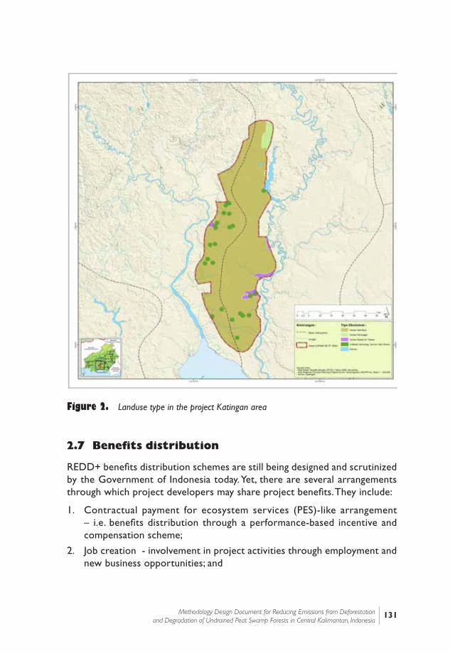
131Methodology Design Document for Reducing Emissions from Deforestation and Degradation of Undrained Peat Swamp Forests in Central Kalimantan, Indonesia
Figure 2. Landuse type in the project Katingan area
2.7 Benefits distribution
REDD+ benefits distribution schemes are still being designed and scrutinized by the Government of Indonesia today. Yet, there are several arrangements through which project developers may share project benefits. They include:
1. Contractual payment for ecosystem services (PES)-like arrangement – i.e. benefits distribution through a performance-based incentive and compensation scheme;
2. Job creation - involvement in project activities through employment and new business opportunities; and

132 Section 2:Social Safeguards
3. Investment in (and/or donation for) community-based economic activities and alternative livelihoods creation (e.g., rattan cultivation, small scale agroforestry and fisheries, development of processing mills, and transfer of skills and technologies).
PES is frequently considered an integral tool for the implementation of REDD+, as it links actions directly to incentives by creating a contractual arrangement. Thus, a PES-like arrangement for benefits distribution can compensate service providers (i.e., local communities) based on their rights and performances. Figure S2 presents the typical PES framewo
In the absence of clear benefits distribution mechanisms, benefitsmay also be distributed through a variety of project activities rather than cash payments.The main activities of the Katingan project are conservation and restoration work of peat swamp forest. The project has been working with communities surrounding the concession area to alleviate pressure on the area through village mapping and alternative livelihood schemes, and also involve them through employment in project activities, such as reforestation and the monitoring of permanent sampling plots. Once REDD+ revenues are generated, the project will increase the scale of support and investment in community-based economic activities and alternative livelihoods programs. Positive effects are expected to multiply as the local economy grows and new investment and employment opportunities arise.

133Methodology Design Document for Reducing Emissions from Deforestation and Degradation of Undrained Peat Swamp Forests in Central Kalimantan, Indonesia
2.8 Monitoring and evaluation of socio-economic impacts
The monitoring and evaluation of socio-economic impacts is an important part of social safeguards because it provides an opportunity to appraise project activities, ensure their efficacy, and make improvements.Project activities should be monitored against clearly defined targets, including, at a minimum:
1. The progress of project activities;
2. Positive impacts on local socio-economy; and
3. Negative impacts on local socio-economy.
Whether project activities have positive or negative impacts on local socio-economic conditionsmay be monitored against five key indicators – human capital, social capital, financial (or economic) capital, physical capital and natural capital (Scoones, 1998). Table S8 summarizes the key socio-economic indicators which are considered crucial for the pursuit of any livelihood activities by communities.
Indicator Description
Human capital Human skills, knowledge, ability to labor in good health and physical capability (i.e., education, training and health care)
Social capital Social resources including social networks, affiliation of certain groups, social norms, trust and relationships
Financial capital Economic assets including cash, loans, savings, cattle and other financial assets
Physical capital Basic infrastructure, equipment and technologies including roads, transport, shelter, energy and communication systems
Natural capital Natural resources such as forests and biodiversity, and environmental services such as hydrological cycle, clean water and air
Further, project activities need to be evaluated against the five indicators as well as pre-determined criteria, including:
1. Environmental sustainability;
2. Land tenure;
3. Livelihoods;
4. Socio-cultural acceptance and community participation; and
5. Financial feasibility.

134 Section 2:Social Safeguards
Results of the evaluation will be useful to communicate lessons learned among all stakeholders, and to identify future requirements and areas for improvement.

135Methodology Design Document for Reducing Emissions from Deforestation and Degradation of Undrained Peat Swamp Forests in Central Kalimantan, Indonesia
Section 3: Environmental Safeguards
Nagoya Biodiversity Summit 2010 set a new international goal of integrating the biodiversity agenda with that of climate change and land degradation. Furthermore, the Cancun Agreements 2010 stipulated that environmental safeguards should be placed in order to ensure that “[REDD+ activities] are used to incentivize the protection and conservation of natural forests and their ecosystem services, and to enhance other social and environmental benefits.”
Box 2 highlights key checkpoints in designing an environmental safeguards methodology. This section further explores environmental safeguards by using a case study from the Katingan Project.
Box 2. Environmental Safeguards Methodology Design Checkpoints• Conduct a preliminary biodiversity assessment • Identification of high value conservation (HCV) areas and species• Participatory ecological / biodiversity assessment• Identification of main drivers of biodiversity loss • HCV mapping
• Develop a sampling plan and permanent monitoring plots• Forest stratification per representative vegetation/forest cover types• Development of permanent sampling plots based on forest stratification• Design of an appropriate sampling plan for periodic biodiversity assessment
• Develop a biodiversity assessment methodology and ecosystem restoration plan• Development of complete and integrated biodiversity database• Development of an appropriate biodiversity assessment methodology• Development of an appropriate ecosystem restoration plan including hydrological
restoration and forest rehabilitation• Ensure biodiversity protection and law enforcement• Risk analysis to identify important areas for protection and enforcement• Development of a fire prevention and control plan and system • Development of a participatory biodiversity monitoring plan• Development of a participatory system network to monitor illegal activities (e.g., illegal
logging and poaching)• Development of appropriate monitoring facilities • Provision of trainings and monitoring equipment to communities• Implementation of QA&QC to assess the proper execution of a work plan
136 Section 3:Environmental Safeguards
3.1 Biodiversity assessment
A rapid assessment of biodiversity and high conservation value (HCV)species was carried out based on field surveys at three sampling sites near the Kemapit, Lemiring and Hantipan rivers located within the Katingan Project area. The assessment identified biodiversity present in the forest, HCV areas containing rare, threatened and endangered species and ecosystems, highlighted threats to the area’s biodiversity and HCV attributes, and proposed priority areas for restoration and conservation.
The biodiversity assessment confirmed a number of HCV attributes present in the Katingan Project area. Furthermore, it is also confirmed that almost the entire area is currently under serious threat due to human activities such as illegal logging, forest conversion for non-forest purposes, fires, gold and coal mining, oil-palm plantation development and hunting. Detailed observations and results from the biodiversity assessment as well as management strategies are presented in the following sections.
3.2 Areas with important levels of biodiversity
3.2.1 HCV assessment
HCV Key Question Results
1.1 Does the Katingan Projectarea have or provide a function to support biodiversity for protected or conservation area within or nearbyarea within or nearby?
Yes
The Katingan Project area is home to the Critically Endangered white-shouldered ibis (Pseudibis davisoni); to globally significant populations of the Endangered Bornean orang-utan (Pongo pygmaeus), Bornean southern gibbon (Hylobates albibarbis) and proboscis monkey (Nasalis larvatus). It is also home to the Endangered Sunda pangolin, flat-headed cat, Storm’s stork, Bornean river turtle, spiny turtle and false gharial. Populations of most of the vulnerable species present in the area, by far, exceed 30 individuals or 10 pairs (Harrison et al, 2010). The area also provides habitats to Critically Endangered flora species such as Shorea balangeran, Dyera lowii/polyphylla, S. uliginosa, Gonystylus bancanus and numerous other floral species populations.
The Key Biodiversity Area (KBA) criteria consider both an area’s vulnerability and its irreplaceability (Langhammer et al., 2007 in Harrison et al, 2010). The vulnerability criterion specifies that an area must have at least one individual
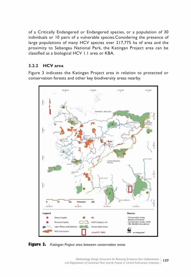
137Methodology Design Document for Reducing Emissions from Deforestation and Degradation of Undrained Peat Swamp Forests in Central Kalimantan, Indonesia
of a Critically Endangered or Endangered species, or a population of 30 individuals or 10 pairs of a vulnerable species.Considering the presence of large populations of many HCV species over 217,775 ha of area and the proximity to Sebangau National Park, the Katingan Project area can be classified as a biological HCV 1.1 area or KBA.
3.2.2 HCV area
Figure 3 indicates the Katingan Project area in relation to protected or conservation forests and other key biodiversity areas nearby.
Figure 3. Katingan Project area between conservation areas

138 Section 3:Environmental Safeguards
3.3 Critically endangered species
3.3.1 HCV assessment
HCV Key Question Results
1.2 Does the Katingan Project area contain critically endangered species?
Yes
Kahui or Shorea belangeran, categorized as a critically endangered (CR)species under the IUCN Red List, was sighted along the Kemapit riverbank during the field survey. White-shouldered ibis (Pseudibis davidsoni), another CR species, has also been observed inside the Katingan Project area. Although none of the mammals sighted during this survey were classified under the CR category,some of the primates categorized as endangered (EN) and endemic to Borneo, were also spotted inside the area. These primates included bekantan (Nasalis larvatus), Orangutan (Pongo pygmaeus) and Bornean Owa (Hylobates albibarbis).
These sightings confirm that the Katingan Project area, especially along riverbanks in primary peat swamp forest, is an important habitat for CR species.
3.3.2 HCV area
Figure 4 indicates the presence and habitats of critically endangered species.

139Methodology Design Document for Reducing Emissions from Deforestation and Degradation of Undrained Peat Swamp Forests in Central Kalimantan, Indonesia
Figure 4. Indication of HCV area in Katingan Project Area
3.4 Areas that contain habitat for viable populations of endangered, restricted range or protected species
HCV Key Question Results
1.3 Does the Katingan Project contain areas used as habitats for viable population of species, which are threatened, restricted ranged or protected?
Yes

140 Section 3:Environmental Safeguards
3.4.1 HCV assessment
A total 387 species of vertebrates inhabit in this region and, due to the largesize of the proposed concession area (217,755 ha), the Katingan Project area is considered to be a critical stronghold for many of the species found here. More than300 species of flora also inhabit the area’s peat swamps. In addition to being home to a large number of species, it is also clear that the area’s swamps are home to important populations of globally threatened species, including one IUCN defined Critically Endangered species (the white-shouldered ibis), 13 Endangered species, 28 Vulnerable species, 63 legally protected species by the Government of Indonesia (GoI), 21 endemic species, and two migrant species (see Table 16).
Table 16. Biodiversity Richness in Katingan Project area
SPECIES
CONSERVATION STATUS
IUCN CITESGoI Endemic Migrant
CR EN VU App.I App.II
Flora 1 3 5 7
Fauna 6 14 9 16 21 7
Avifauna 1 1 6 2 16 38 3 2
Reptilian 3 3 1 6 4 4
Total 2 13 28 12 38 63 21 2
The Key Biodiversity Area (KBA) criteria consider both an area’s vulnerability and its irreplaceability (Langhammer et al., 2007 in Harrison et al, 2010). The vulnerability criterion specifies that an area must have at least one individual of a Critically Endangered or Endangered species, or a population of 30 individuals or 10 pairs of a vulnerable species.Thus, the Katingan Project area clearly satisfies the KBA criteria on the number of count. In particular, the biodiversity assessment demonstrates that the area is home to viable populations of the Bornean orangutan, southern gibbon and proboscis monkey.
3.4.2 HCV area
Figure 5 indicates the presence and habitats of viable population of species, which are threatened, restricted range or protected inside the Katingan Project area.
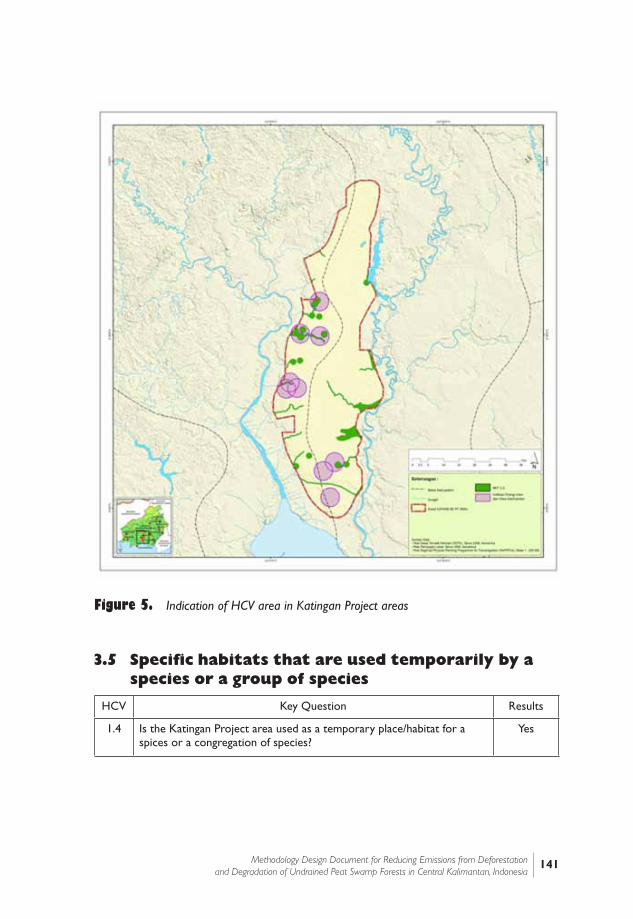
141Methodology Design Document for Reducing Emissions from Deforestation and Degradation of Undrained Peat Swamp Forests in Central Kalimantan, Indonesia
Figure 5. Indication of HCV area in Katingan Project areas
3.5 Specific habitats that are used temporarily by a species or a group of species
HCV Key Question Results
1.4 Is the Katingan Project area used as a temporary place/habitat for a spices or a congregation of species?
Yes

142 Section 3:Environmental Safeguards
3.5.1 HCV assessment
There are two species of migrant birds; namely, Common sandpiper (Actitis hypoleucos) and Barn swallow (Hirundo rustica). Common sandpiper is identified as a vulnerable species in some states of Australia, and also one of the species, to which the Agreement on the Conservation of African-Eurasian Migratory Water Birds (AEWA) applies.These two bird species depend heavily on watershed areas inside and around the Katingan Project area.
3.5.2 HCV area
Figure 6 indicates the habitats of the migratory species inside the Katingan Project area.
Figure 6. Indication of HCV area of migatory species in Katingan Project Area
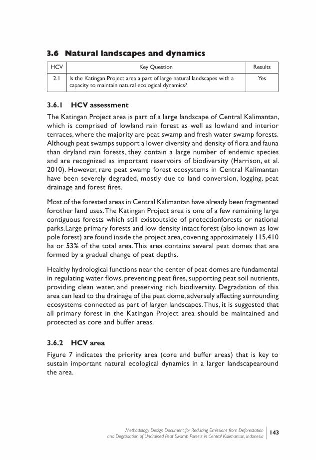
143Methodology Design Document for Reducing Emissions from Deforestation and Degradation of Undrained Peat Swamp Forests in Central Kalimantan, Indonesia
3.6 Natural landscapes and dynamics
HCV Key Question Results
2.1 Is the Katingan Project area a part of large natural landscapes with a capacity to maintain natural ecological dynamics?
Yes
3.6.1 HCV assessment
The Katingan Project area is part of a large landscape of Central Kalimantan, which is comprised of lowland rain forest as well as lowland and interior terraces, where the majority are peat swamp and fresh water swamp forests.Although peat swamps support a lower diversity and density of flora and fauna than dryland rain forests, they contain a large number of endemic species and are recognized as important reservoirs of biodiversity (Harrison, et al. 2010). However, rare peat swamp forest ecosystems in Central Kalimantan have been severely degraded, mostly due to land conversion, logging, peat drainage and forest fires.
Most of the forested areas in Central Kalimantan have already been fragmented forother land uses. The Katingan Project area is one of a few remaining large contiguous forests which still existoutside of protectionforests or national parks.Large primary forests and low density intact forest (also known as low pole forest) are found inside the project area, covering approximately 115,410 ha or 53% of the total area. This area contains several peat domes that are formed by a gradual change of peat depths.
Healthy hydrological functions near the center of peat domes are fundamental in regulating water flows, preventing peat fires, supporting peat soil nutrients, providing clean water, and preserving rich biodiversity. Degradation of this area can lead to the drainage of the peat dome, adversely affecting surrounding ecosystems connected as part of larger landscapes. Thus, it is suggested that all primary forest in the Katingan Project area should be maintained and protected as core and buffer areas.
3.6.2 HCV area
Figure 7 indicates the priority area (core and buffer areas) that is key to sustain important natural ecological dynamics in a larger landscapearound the area.
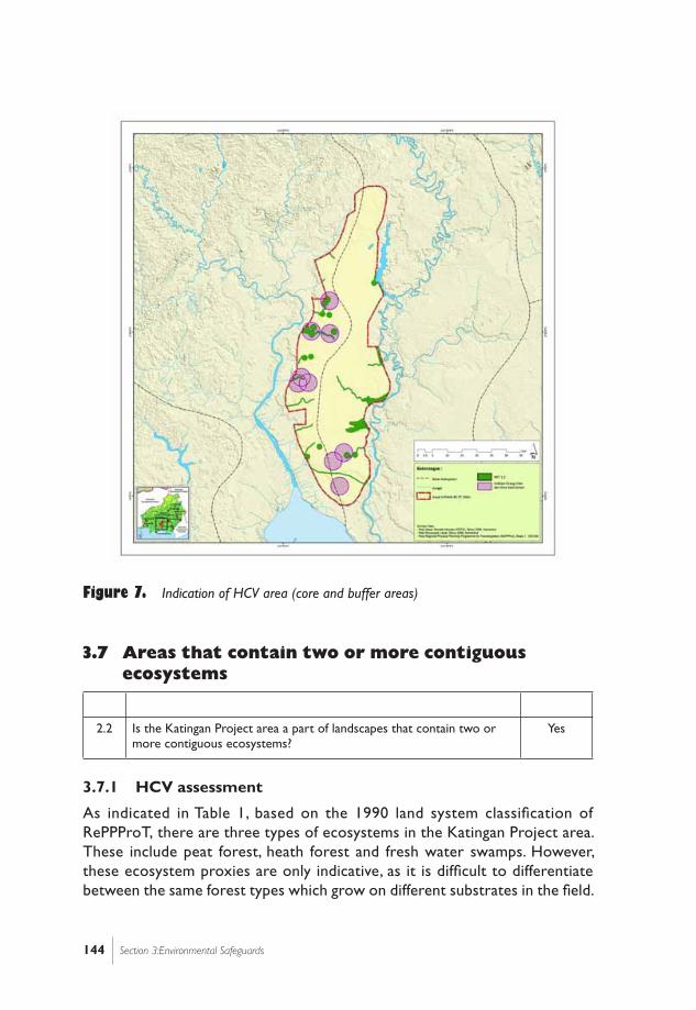
144 Section 3:Environmental Safeguards
Figure 7. Indication of HCV area (core and buffer areas)
3.7 Areas that contain two or more contiguous ecosystems
HCV Key Question Results
2.2 Is the Katingan Project area a part of landscapes that contain two or more contiguous ecosystems?
Yes
3.7.1 HCV assessment
As indicated in Table 1, based on the 1990 land system classification of RePPProT, there are three types of ecosystems in the Katingan Project area. These include peat forest, heath forest and fresh water swamps. However, these ecosystem proxies are only indicative, as it is difficult to differentiate between the same forest types which grow on different substrates in the field.

145Methodology Design Document for Reducing Emissions from Deforestation and Degradation of Undrained Peat Swamp Forests in Central Kalimantan, Indonesia
3.7.2 HCV area
Figure 8 indicates types of ecosystems found in the Katingan Project area. The large orange-colored area is classified as peat forest, the purple area as heath forest and the pink area as fresh water swamps.
Figure 8. Types of ecosystem in the Katingan Project Areas
3.8 Areas that contain representative populations of most naturally occurring species
HCV Key Question Results
2.3 Is the Katingan Project area a part of landscapes containing population of most naturally occurring species?
Yes
146 Section 3:Environmental Safeguards
3.8.1 HCV assessment
The Katingan Project area is dominated by peat swamp forests and supports a significant population of HCV species includingcritically endangered kahui (Shorea belangeran) and white-shouldered ibis (Pseudibisdavidsoni). Similarly, a number of threatened and endangered primates, including orangutan (Pongo pygmaeus), bornean owa (Hylobates albibarbis) and bekantan (Nasalis larvatus),also exist as observed in some of the sampling sites during the survey. Top predator species such as clouded leopard (Neofelisnebulosa), crocodile (Crocodylussp.), eagles and owls amongother species are also found in the area.
Katingan’s peat forests constitute approximately 7.6% of the remaining peat swamp ecosystems in Central Kalimantan. A large stretch of natural habitats and sub-habitats contain primary forests and low pole forestswithin the peat swamp ecosystem. Considering the large contiguous area of the Katingan Project, it is very likely that a viable population of these endangered and/or endemic floral and faunal species occur in large numbers.
3.8.2 HCV area
Figure 9 indicates primary habitats and sub-habitats inside the Katingan Project area, which are important for a viable population of HCV species.

147Methodology Design Document for Reducing Emissions from Deforestation and Degradation of Undrained Peat Swamp Forests in Central Kalimantan, Indonesia
Figure 9. Primary habitats and sub-habitats inside the Katingan Project area
3.9 Rare or endangered ecosystems
HCV Key Question Results
3 Is the Katingan Project area a part of landscapes containing rare or endangered ecosystems?
Yes
3.9.1 HCV assessment
The Katingan Project area is considered to contain rare ecosystems according to the HCVF identification guidelines for Indonesia (2008). The area’s
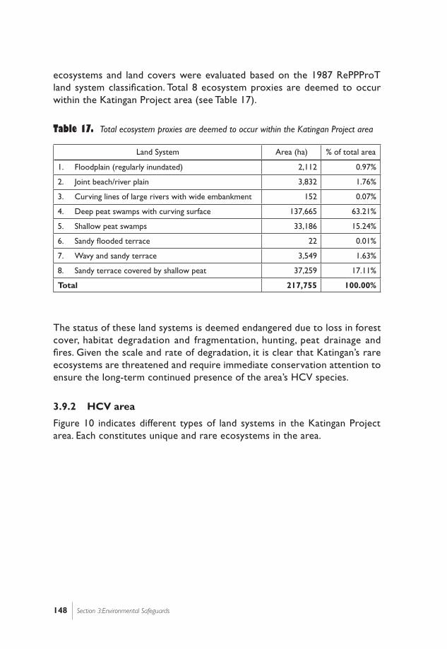
148 Section 3:Environmental Safeguards
ecosystems and land covers were evaluated based on the 1987 RePPProT land system classification. Total 8 ecosystem proxies are deemed to occur within the Katingan Project area (see Table 17).
Table 17. Total ecosystem proxies are deemed to occur within the Katingan Project area
Land System Area (ha) % of total area
1. Floodplain (regularly inundated) 2,112 0.97%
2. Joint beach/river plain 3,832 1.76%
3. Curving lines of large rivers with wide embankment 152 0.07%
4. Deep peat swamps with curving surface 137,665 63.21%
5. Shallow peat swamps 33,186 15.24%
6. Sandy flooded terrace 22 0.01%
7. Wavy and sandy terrace 3,549 1.63%
8. Sandy terrace covered by shallow peat 37,259 17.11%
Total 217,755 100.00%
The status of these land systems is deemed endangered due to loss in forest cover, habitat degradation and fragmentation, hunting, peat drainage and fires. Given the scale and rate of degradation, it is clear that Katingan’s rare ecosystems are threatened and require immediate conservation attention to ensure the long-term continued presence of the area’s HCV species.
3.9.2 HCV area
Figure 10 indicates different types of land systems in the Katingan Project area. Each constitutes unique and rare ecosystems in the area.
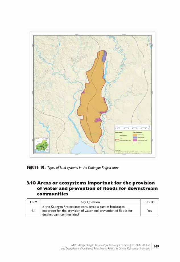
149Methodology Design Document for Reducing Emissions from Deforestation and Degradation of Undrained Peat Swamp Forests in Central Kalimantan, Indonesia
Figure 10. Types of land systems in the Katingan Project area
3.10 Areas or ecosystems important for the provision of water and prevention of floods for downstream communities
HCV Key Question Results
4.1Is the Katingan Project area considered a part of landscapes important for the provision of water and prevention of floods for downstream communities?
Yes
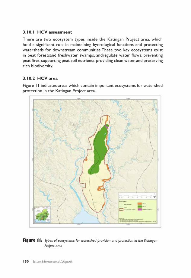
150 Section 3:Environmental Safeguards
3.10.1 HCV assessment
There are two ecosystem types inside the Katingan Project area, which hold a significant role in maintaining hydrological functions and protecting watersheds for downstream communities.These two key ecosystems exist in peat forestsand freshwater swamps, andregulate water flows, preventing peat fires, supporting peat soil nutrients, providing clean water, and preserving rich biodiversity.
3.10.2 HCV area
Figure 11 indicates areas which contain important ecosystems for watershed protection in the Katingan Project area.
Figure 11. Types of ecosystems for watershed provision and protection in the Katingan Project area
151Methodology Design Document for Reducing Emissions from Deforestation and Degradation of Undrained Peat Swamp Forests in Central Kalimantan, Indonesia
3.11 Areas important for the prevention of erosion and sedimentation
HCV Key Question Results
4.2 Does the Katingan Project area hold areas important for the prevention of erosion and sedimentation for downstream communities?
No
3.11.1 HCV assessment
Because of the low altitude and flat topography ofthe Katingan Project area, erosion and sedimentation are not likely to occur.
There is an areas that function as a natural break to the spread of forest or ground fires
HCV Key Question Results
4.3 Is the Katingan Project area a part of landscapes that function as a natural break to the spread of forest or ground fire?
Yes
3.11.2 HCV assessment
The Katingan Project area is dominated by peat forest and fresh water swamp ecosystems. These two types of swamp forests play a significant role as natural buffers to prevent the spread of forest or ground fires. Interviews with local communities and remote sensing analyses have confirmed the occurrence of peat forest fires inside the project area, particularly in non-forested areas as well as along a large canal which connects between the Mentaya and Katingan Rivers. Figure 12 shows hotspots observed from 1993 through 2008 in and around the project area. Most parts of the concession area have survived from devastating peat fires, and this clearly suggests that the area’s unique ecosystems provide a critical function to prevent and control fires.

152 Section 3:Environmental Safeguards
Figure 12. Hotspots observed from 1993 through 2008 in and around the project area
3.11.3 HCV area
Figure 13 (shown in pink lines) indicates areas which are important as natural breaks to the spread of forest and/or ground fires in the Katingan Project area.
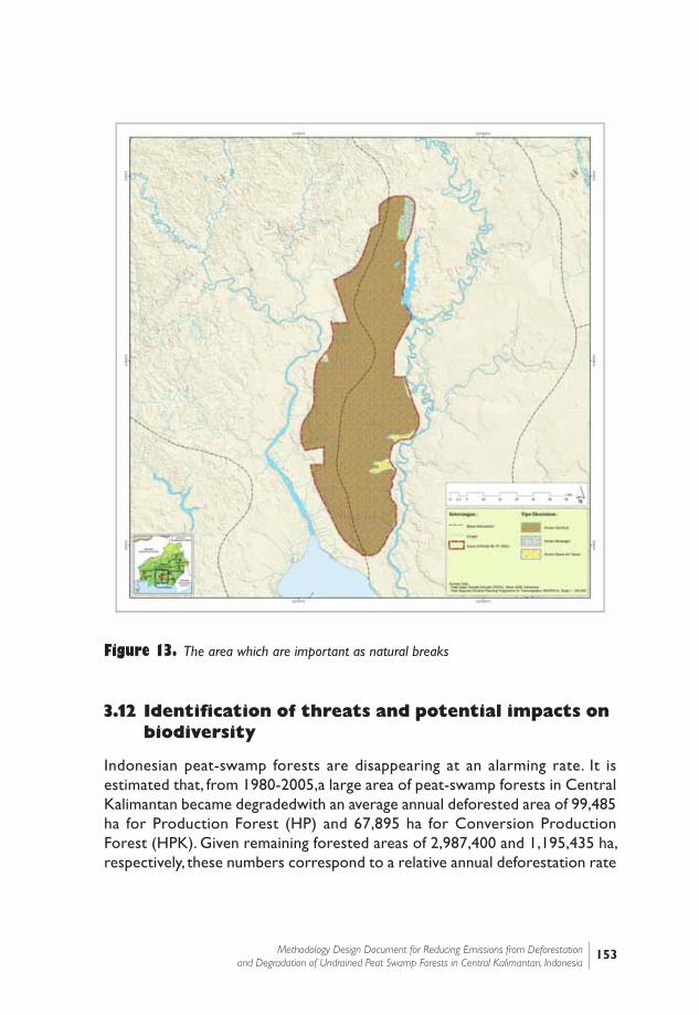
153Methodology Design Document for Reducing Emissions from Deforestation and Degradation of Undrained Peat Swamp Forests in Central Kalimantan, Indonesia
Figure 13. The area which are important as natural breaks
3.12 Identification of threats and potential impacts on biodiversity
Indonesian peat-swamp forests are disappearing at an alarming rate. It is estimated that, from 1980-2005,a large area of peat-swamp forests in Central Kalimantan became degradedwith an average annual deforested area of 99,485 ha for Production Forest (HP) and 67,895 ha for Conversion Production Forest (HPK). Given remaining forested areas of 2,987,400 and 1,195,435 ha, respectively, these numbers correspond to a relative annual deforestation rate

of 3.33 % for HP and 5.68 % for HPK areas across Central Kalimantan23. The peat swamp forest of the Katingan Project area is no exception.
The main drivers of deforestation in and around the Katingan Project area continue to be forest conversion into plantations and mining, small-scale farming particularly through shifting cultivation and illegal logging (both commercial and subsistence). Furthermore, forest degradation due to peat drainage and fires poses serious threats to the area’s biodiversity and the integrity of ecosystems. Table 18 shows a list of major threats to the HCV attributes observed within and/or around the Katingan Project area.
Table 18. List of major threats to the HCV
No Source of Threats 1.1 1.2 1.3 1.4 2.1 2.2 2.3 3 4.1 4.2 4.3
1 Illegal logging + + + + + + + +
2 Forest conversion (i.e., oil palm, rubber and other monoculture plantations)
+ + + + + + + + + +
3 Mining (legal and illegal) + + + + + + +
4 Peat drainage + + + + + + + + + +
5 Fire + + + + + + + + +
6 Hunting + + +
7 Fishing + + + +
8 Harvesting of non-timber forest products + +
10 Revisions of Regency and/or Provincial Spatial Plans
+ + + + + + +
11 Charcoal Production + +
Apparently, the greatest threat to the area’s biodiversity is forest conversion,whichinevitably resultsfrom the clearing of large tract of forested lands. However, as the above table indicates, unsustainable forest resources management can also pose multiple impacts and serious threats to biodiversity and HCV areas. Most local communities depend on forest resources (e.g., rattan, fish, timber, rubber and jelutung) to support their livelihoods. Thus, sustaining healthy ecosystems is crucial not only for the protection of biodiversity but also as a way to safeguard social benefits.
23] These numbers were estimated by the Terra Global Capital using the historical deforestation data of the Central Kalimantan Province.

155Methodology Design Document for Reducing Emissions from Deforestation and Degradation of Undrained Peat Swamp Forests in Central Kalimantan, Indonesia
3.13 Management strategies to maintain HCVF
Comprehensive biodiversity management strategies have been developed for the Katingan Project area in order to conserve and maintain HCV species and areas. These strategies include:
1) Forest protection;
2) Restoration of degraded lands;
3) In-situ and ex-situ conservation; and
4) Collaborative biodiversity management.
Detailed strategies and plans are discussed in the following sections. Also, a list of management strategy for each HCV attribute is provided in Annex 5.
3.13.1 Forest protection
The maintenance of certain HCVs requires the protection of forests, particularly those with high concentration of HCV attributes. Strategies for forest safeguards include:
1. To providesanctuaries for species which are sensitive to ecological disturbances;
2. To ensure connectivity among remnant primary forest patches and conservation set-asides;
3. To prevent the degradation of water quality;
4. To maintain social HCVs as they related to forest protection;
5. To maintain areas important for a temporary congregation of HCV species;
6. To maintain a source of seedlings to promote forest rehabilitation efforts;
7. To monitor forest ecological dynamics by surveying permanent sampling plots;
8. To maintain a representative sample of each ecosystem in its natural state; and
9. To protect and secure suitable habitats for endangered species, particularly for orangutans, proboscis monkeys and Bornean gibbons.
3.13.2 Restoration of degraded lands
The objective of forest restoration activities is to restore and enhance forest and soil conditions which have been degraded over time by both human
156 Acronyms
and natural causes. Degradation of peatlands typically occurs near human settlements, agricultural lands, canals, roads and fire prone areas mainly because of decreased water levels as a result of peat drainage. Restoration strategies include the maintenance and enhancement of forest and non-forest areas, particularly around:
1. Canals (including abandoned canals);
2. Logging tracks;
3. Logged-over forest;
4. Abandoned infrastructures;
5. Abandoned shifting cultivation areas;
6. Burnt areas (post forest fire areas); and
7. Open / barren lands.
Restoration projects should also involve local communities who are likely to be affected by planned activities. For example, canals have long been used by many local people as their only transport routes to access to forest areas. Any activities (e.g., construction of dams to block canals) which may affect their access to forests must be planned carefully based on mutual agreement.
3.13.3 In-situ and ex-situ conservation
The main strategy to deal with the threat of floral and faunal extinction in Indonesia is through in-situ and ex-situ conservation. In-situ conservation refers to the conservation of ecosystems and natural habitats and the maintenance and recovery of viable populations of species in their natural surroundings (FAO 2010). Ex-situ conservation is defined as measures taken to safeguard biodiversity outside their natural habitats, and is generally used to protect or recover populations or individuals that are presently or potentially under the threat of extinction.
As a main strategy to conserve biodiversity in the Katingan Project area, integrated in-situ and ex-situ conservation methodologieswill be adopted as mutually supporting approaches.Protection and conservation of rare, threatened and endangered flora and faunal species, such as orangutans, proboscis monkeys and gibbons,will be managed though in-situ conservation in order to restore important habitats within the Katingan Project area. Ex-situ conservation will be implemented to rehabilitate, nurture and preserve threatened species in small numbers in order to safeguard them from potential extinction.
157Methodology Design Document for Reducing Emissions from Deforestation and Degradation of Undrained Peat Swamp Forests in Central Kalimantan, Indonesia
3.13.4 Collaborative biodiversity management
Collaborative biodiversity management (CBM) is a dynamic approach used to converge the interests of different stakeholders including government agencies, concession companies, non-governmental organizations (NGOs) and forest-dependent communities in achieving sustainable and equitable forest resource management. CBM aims to:
1. Reduce conflicts between concession companies and local people over access to and use of forest resources;
2. Protect sites of cultural, spiritual and subsistence importance for local communities;
3. Ensure equitable distribution of benefits from forestry operations;
4. Increase coordination among stakeholders on community development issues;
5. Increase community participation in forest management and monitoring activities;
6. Prevent illegal activities within concession boundaries by local people and/or outsiders.
In order to ensure sustainable management of biodiversity, CBM should be adopted as one of the environmental safeguard strategies. Such a collaborative measurement will ensure the equitable management of forest resources to reflect diverse requirements of all forest users, and will lead to long-term partnerships with all stakeholders in decision-making processes.

158 Acronyms

159Methodology Design Document for Reducing Emissions from Deforestation and Degradation of Undrained Peat Swamp Forests in Central Kalimantan, Indonesia
References
Achard, F., H.D. Eva, H.J. Stibig, P. Mayaux, J. Gallego, T. Richards, and J.P. Malingreau. 2002. Determination of deforestation rates of the world's humid tropical forests. Science 297:999-1002.
Angelsen, A., and D. Kaimowitz. 1999. Rethinking the causes of deforestation: Lessons from economic models. World Bank Research Observer 14:73-98.
Aukland, L., P.M. Costa, and S. Brown. 2003. A conceptual framework and its application for addressing leakage; the case of avoided deforestation. Climate Policy 3:123–136.
Boer, R., U.R. Wasrin, Perdinan, Hendri, B. D. Dasanto, W. Makundi, J. Hero, M. Ridwan, and N. Masripatin. 2006. Assessment Of Carbon Leakage In Multiple Carbon-Sink Projects: A Case Study In Jambi Province, Indonesia.
Brown, S., F. Achard, and B. Braatz. 2008. Reducing greenhouse gas emissions from deforestation and degradation in developing countries: a sourcebook of methods and procedures for monitoring, measuring and reporting GOFC-GOLD Project Office, Alberta, Canada.
Chambers, J, Higuchi, N, Schimel, J. P., Ferreira, L. V., Melack, J. M. 2000. Decomposition and carbon cycling of dead trees in tropical forests of the central Amazon. Oecologia, 122: 380-388.
Chave, J., Andalo, C., Brown, S., and Cairns, M. A., 2005.Tree Allometry and Improved Estimation of Carbon Stocks and Balance in Tropical Forests, Oecologia 145: 87-99.
Chomitz, K.M., P. Buys, G. De Luca, T.S. Thomas, and S. Wertz-Kanounnikoff. 2006. At loggerheads. Agricultural Expansion, Poverty Reduction, and Environment in the Tropical Forests World Bank, Washington, DC.
Cochran, W.G. 1977. Sampling Techniques. Wiley. New York.
Colchester M. (2010).Free, Prior and Informed Consent: Making FPIC work for forests and peoples. The Forests Dialogue, Connecticut, The United States.
Congalton, R.G. 1991. A Review of Assessing the Accuracy of Classifications of Remotely Sensed Data. Remote Sensing of Environment 37:35-46.
160 References
Couwenberg, J., Dommain, R. & Joosten, H. 2010. Greenhouse gas fluxes from tropical peatlands in south-east Asia. Global Change Biology 16: 1715– 1732.
Crutzen, P.J., I. Aselmann, and W. Seiler. 1986. Methane production by domestic animals, wild ruminants, other herbivorous fauna and humans. Tellus 38B:271–284.
De Jong, B.H.J., E. Esquivel Bazan, and S. Quechulpa Montalvo. 2007. Application of the “Climafor” baseline to determine leakage; the case of Scolel Te. Mitigation and Adaptation Strategies for Global Change.
DNPI. (2010). Indonesia’s Greenhouse Gas Abatement Cost Curve. Jakarta, Indonesia.
Echeverria, C., Coomes, D.A., Hall, M., Newton, A.C. 2008.Spatially explicit models to analyze forest loss and fragmentation between 1976 and 2020 in southern Chile. Ecological Modeling 212: 439-449.
Freese, F. 1962.Elementary Forest Sampling. USDA Handbook 232 GPO Washington, DC.
Freudenberger, K.S. 1994. Tree and land tenure rapid appraisal tools.Food and Agricultural Organization of the United Nations. Rome.
Gnatowski T., Szatyowicz, J. and Brandyk, T. 2002.Effect of peat decomposition on the capillary rise in peat-moorish soils from the Biebrza River Valley. Int. Agrophysics 16: 97-102
Harmon, M. E. and J. Sexton. 1996. Guidelines for Measurements of Woody Detritus in Forest Ecosystems. US LTER Publication No. 20. US LTER Network Office, University of Washington,, Seattle, WA, USA.
Hamburg, S.P. 2000. Simple rule for measuring changes in ecosystem carbon in forestry-offset projects. Mitigation and Adaptation Strategies for Global Change 5:25-37.
Harrison M. E., Hendri, Dragiewicz M. L., Krisno, Cheyne S. M. and Husson S. J. (2010). Baseline Biodiversity and Ape Population Assessment and Preliminary Monitoring Protocol in the Katingan Peat Swamp, Central Kalimantan, Indonesia. Report produced by the Orangutan Tropical Peatland Project for PT. Rimba Makmur Utama / PT. Starling Asia, Palangka Raya, Indonesia.
161Methodology Design Document for Reducing Emissions from Deforestation and Degradation of Undrained Peat Swamp Forests in Central Kalimantan, Indonesia
Harrison M. E., Kursani, Santiano, Hendri, Purwanto A. and Husson S. J. (2011). Baseline Flora Assessment and Preliminary Monitoring Protocol in the Katingan Peat Swamp, Central Kalimantan, Indonesia. Report produced by the Orangutan Tropical Peatland Project for PT. Rimba Makmur Utama / PT. Starling Asia, Palangka Raya, Indonesia.
Hooijer, A., M. Silvius, H. Wösten and S. Page (2006). PEAT-CO2: Assessment of CO2 Emissions from Drained Peatlands in SE Asia. Delft Hydraulics report Q3943.
Hoover, C.M. (ed). 2008. Field Measurements for Forest Carbon Monitoring: A Landscape-Scale Approach. Springer, New York. Hardcover. ISBN 978-1-4020-8505-5.
IPCC. 2003a. Good Practice Guidance for Land Use, Land Use Change and Forestry Projects (GPG-LULUCF) Intergovernmental Panel on Climate Change, Geneva, Switzerland.
IPCC. 2003b. Definitions and Methodological Options to Inventory Emissions from Direct Human-Induced Degradation of Forests and Devegetation of Other Vegetation Types Intergovernmental Panel on Climate Change, Geneva, Switzerland.
IPCC. 2006. Good Practice Guidance for National Greenhouse Gas Inventories. Chapter 4: Agriculture, Forestry, And Other Land Uses (AFOLU). Intergovernmental Panel On Climate Change, Geneva, Switzerland.
ISO. 2006. ISO 14064-2:2006 - Greenhouse gases — Part 2: Specification with guidance at the project level for quantification, monitoring and reporting of greenhouse gas emission reductions or removal enhancements. ISO, Geneva, Switzerland.
Ketterings, M. Q., R. Coe, M. v. Noordwijk, Y. Ambagau and C. A. Palm. 2001. Reducing Uncertainty in the Use of Allometric Biomass Equation for Predicting Above Ground Tree Biomass in Mixed Secondary Forest. Forest Ecology and Management 146: 199-209.
Kish, L. 1995. Survey Sampling. Wiley Interscience.
Krejcie, R.V. and Morgan, D.W. 1970. Determining sample size for research activities. Educational and psychological measurement 30: 607-610.
Lambin, E.F. 1997. Modelling and monitoring land-cover change processes in tropical regions. Progress in Physical Geography 21:375-393.

162 References
Miles, L., and V. Kapos. 2008. Reducing greenhouse gas emissions from deforestation and forest degradation: Global land-use implications. Science 320:1454-1455.
Neeff, T., H. von Luepke, and D. Schoene. 2006. Forests and climate change working paper 4: choosing a forest definition for the clean development mechanism. FAO, Rome, Italy.
Olander, L.P., B.C. Murray, M. Steininger, and H. Gibbs. 2006. Establishing Credible Baselines for Quantifying Avoided Carbon Emissions from Reduced Deforestation and Forest Degradation Duke University, Durham, NC.
Pearson, T., S. Walker, and S. Brown. 2005. Sourcebook for Land use, land-use change and forestry projects BioCarbon Fund of the World Bank, Washington, DC.
Pontius, R.G. 2002. Statistical methods to partition effects of quantity and location during comparison of categorical maps at multiple resolutions. Photogrammetric Engineering and Remote Sensing 68:1041-1049.
Reyes, G., S. Brown, J. Chapman, and A.E. Lugo. 1992. Wood densities of tropical tree species USDA, Washington, DC.
Sathaye, J.A., and K. Andrasko. 2007. Land use change and forestry climate project regional baselines: a review. Mitigation and Adaptation Strategies in Global Change 12:971–1000.
Satrio A.E., Gandaseca, S., Ahmed O.H., Majid, N.M. 2009.Effect of Logging Operation on Soil Carbon Storage of a Tropical Peat Swamp Forest. American Journal of Environmental Sciences 5:748:752.
Schlamadinger, B., L. Ciccarese, M. Dutschke, P.M. Fearnside, S. Brown, and D. Murdiyarso. 2005. Should we include avoidance of deforestation in the international response to climate change?,In D. Murdiyarso and H. Herawati, eds. Carbon forestry: who will benefit? Proceedings of the Workshop on Carbon Sequestration and Sustainable Livelihoods, Bogor, Indonesia.
Scoones, I. (1998). Sustainable rural livelihoods: A framework for analysis. IDS Working Paper. No.72. Brighton: IDS.
Serneels, S., Lambin, E., 2001. Proximate causes of land-cover change in Narok District, Kenya: a spatial statistical model. Agriculture, Ecosystems and Environment 85, 65–81.

163Methodology Design Document for Reducing Emissions from Deforestation and Degradation of Undrained Peat Swamp Forests in Central Kalimantan, Indonesia
Smith E. M., Gryze S.D., Kusumaatmadja R., Darusman T., and Hardiono M. (2011). Standard Operation Procedure (SOP) for Field Measurements: Measurement of peat depth, installation of permanent watertable monitoring points, installation of permanent peat subsidence points and installation of permanent forest inventory plots for an avoided peatland conversion project, in Central Kalimantan Province, Indonesia. Version 5-0. Terra Global Capital and Starling Resources.
Sharma B., Gryze S. D., Smith E. M., Silverman J. (2011). Standard Operations Procedure for Allometric Equation Verification: Procedure to verify allometric equations for an avoided peatland conversion project in Central Kalimantan Province, Indonesia. Version 1-0. Terra Global Capital and Starling Resources.
Sulistiyanto, Y. (2004). Nutrient dynamics in different sub-types of peat swamp forest in Central Kalimantan, Indonesia. PhD Thesis. University of Nottingham. Nottingham. 388 p.
Terra Global Capital. (2010). Baseline and Monitoring Methodology for Avoiding Planned Deforestation of Undrained Peat Swamp Forests. Draft version 2.0. California.
Thompson, S.K. 2000. Sampling. John Wiley and Sons, Hoboken, NJ.
Top, N., Mizoue, N., Kai, S., Nakao, T. 2004 Variation in woodfuel consumption patterns in response to forest availability in Kampong Thom Province, Cambodia. Biomass and Bioenergy 27: 57-68
Tropenbos. (2008). Panduan Identifikasi Kawasan Bernilai Konservasi Tinggi di Indonesia.Konsorsium Revisi HCV Toolkit Indonesia.Tropenbos International Indonesia Programme.
UN [United Nations]. 2008. Designing Household Survey Samples: Practical Guidelines. Department of Economics and Social Affairs, Statistics Division. ST/ESA/STAT/SER.F/98. United Nations. New York.
Van Wagner, C. E. 1968. The line intersect Method in forest Fuel Sampling. Forest Science 14:20-26.
Verburg, P.H., K.P. Overmars, and N. Witte. 2004. Accessibility and land-use patterns at the forest fringe in the northeastern part of the Philippines. The Geographical Journal 170:238–255.

164 References
Williams, N.G., McDonnell, M.J., and Seager, E. 2005. Factors influencing the loss of an endangered ecosystem in an urbanizing landscape: a case study of native grasslands from Melbourne, Australia. Landscape and Urban Planning 71, 35–49.
Winjum, J.K., Brown, S., Schlamadinger, B. 1998. Forest harvests and wood products: sources and sinks of atmospheric carbon dioxide. Forest Science 44:272-284
Wösten, H., Clymans, E., Page, S.E., Rieley, J.O. Limin, S.H. 2008. Peat–water interrelationships in a tropical peatland ecosystem in Southeast Asia. Catena. 73: 212-224.
| 165Development and Testing of a Carbon MRV Methodology and Monitoring Plan: Allometric Equation Development, Forest Biomass Mapping (Aboveground Carbon Stock), Water Level and Peat Anaysis (Below Ground Carbon Stock)
Annex 1: Standard Operation Procedure for Field
Measurements
Measurement of peat depth, installation of permanent watertable monitoring points, installation of permanent peat subsidence points and installation of permanent forest inventory plots for an
avoided peatland conversion project, in Central Kalimantan Province, Indonesia
Version 7-0

166 | Annex I: Standard Operation Procedure for Field Measurements
Acronyms and Definitions
cm centimeterDBH Diameter at Breast Height (1.3 m above the ground)GPS Global Positioning System (handheld device)m meter PVC Polyvinyl chloride, (a type of plastic easily used for permanent watertable measuring
point and subsidence point installation kg KilogramUTM Universal Transverse Mercator (Set to UTM49S for Katingan District, Central
Kalimantan Province, Indonesia)
Definitions
Forest Wooded land with a tree crown cover of at least 10 %, of at least 1 ha in size, and a minimum tree height of 5 m.
Peat An accumulation of partially decayed vegetation matter of at least 0.5 meters thick at ground surface or below water level.

| 167Development and Testing of a Carbon MRV Methodology and Monitoring Plan: Allometric Equation Development, Forest Biomass Mapping (Aboveground Carbon Stock), Water Level and Peat Anaysis (Below Ground Carbon Stock)
1. Overview and Sampling Design
1.1 Overview
The sampling plan consists of a four different monitoring components:
1. Installing and measuring a permanent watertable monitoring point. Carbon dioxide emissions from peat are linearly related to the depth of the watertable1. Continuous water-table measurements at several positions in the project area are very important. Even in native forests, there can be substantial gas fluxes. Therefore, the watertable must be carefully monitored during the project period within the project area. Watertable monitoring occurs through the installation of permeable (PVC) tubes in the peat, and measuring the water level from the surface within the tube.
2. Installing and measuring a permanent peat subsidence monitoring point. Upon gradual decomposition of the peat layer, a decrease in depth of the peat layer and an eventual collapse of the peat dome will occur. Monitoring peat subsidence is a direct way to quantify the amount of peat that has been decomposed by measuring the decrease in the thickness of the peat layer.
3. Measuring peat depth. Peat depth varies within the project area. Carbon credits are based on the avoidance of emissions from peat oxidation, which is constrained by the total mass of peat that is present in the project. The latter can be quantified by measuring the depth of the peat layer at different points within the project area.
4. Establishing and measuring permanent forest inventory plots. Permanent forest inventory plots are a standard and generally accepted way to quantify the biomass in living and dead trees in forest systems. Permanent plots are adequate to quantify relatively minor changes in forest biomass.
These four different components are combined on three different plot types:
1. Temporary peat-depth measurement points, where the peat depth and depth of the watertable are measured, but no permanent watertable monitoring point or peat subsidence measurement point is installed.
2. Permanent peat-depth (subsidence) and watertable monitoringpoints, where a permanent watertable monitoring point and a peat subsidence point are installed in close proximity to each other. Permanent peat subsidence points should be installed 2 meters north of the watertable monitoring point.
3. Full measurement plots, combines all of plot type 2 together with a biomass inventory point. Due to the substantial amount of field work necessary to install all of the plot types, the installation is spread over the first four years of the project. Only after four years, all of the measurement plots will be available for continuous monitoring. This concept is integrated within the methodology accompanying this SOP.
1Hokkaidouniversity has flux towers in non‐forest areas in Kalampangan and in forest area in Sebangau near the field station, for which it has developed relations between water‐table depth and gas fluxes. These relations can be used for the Katingan project. Within the native forest of the project area, it was recommended to install a flux tower (cost of equipment = about USD 30,000). However, it is not necessary to have the flux tower installed before submission of the PD.
168 | Annex I: Standard Operation Procedure for Field Measurements
Additionally to the sampling components outlined above, three additional measurements must be carried out:
• The validity of the allometric equation relating tree diameter and/or height to tree mass must be explicitly validated using about 10 destructively harvested trees. Prof. Osaki-san has an allometric equation for the forest types within Katingan based on the Kalampangan research site2.
• The carbon content of peat can vary substantially with depth within a peat profile. Therefore, it is essential to measure the carbon content of peat at different depths. Within the Katingan project, the carbon content of 3-4 profiles should be measured at 3-4 depths.
• Rainfall must be measured at several locations within the project area.
1.2 Sampling Design
i. Overview and Justification
The density and limited accessibility of the Katingan forest make a fully randomized sampling design impossible. In addition, the project area contains one or several peat domes that are characterized by gradually changing peat depths. Such gradual changes can easily be missed by a completely randomized design. Since the quickest way of accessing the forest is using waterways, a hybrid transect and (semi-) random sampling design is proposed. Such a design is believed to optimal given the geography of the peat, constraints in accessibility and the work-load of the field crews. The hybrid design combines the merits of transects, which are the ability to monitor gradual changes across different distances from the center of the peat dome, and the advantages of a (semi-)randomized design, which is the minimization of statistical bias.
• Only peat depth measurement points (“D points”) are located along four transects. The two proposed new transects will have an average distance of 250 m between the sample points. Near the middle of the peat dome, the distance between point should be greater, e.g., 500 m or 1 km since the change of the depth in the middle of the dome usually small. 160 samples will be located along four transects. An additional 40 samples will be collected over years two and three for a total of 200 points. Year two and three samples will be located per statistical analysis of the year one results.
• The permanent watertable and peat subsidence sampling points are located according to an adaptive transect design. More specifically, permanent watertable and peat subsidence points are located across four east-west transects, with an average distance of 250 m between the points. To even the work-load of the field crews, only 25% of the points along the transect will be installed in the first year, with 25% more every following year. The location of the future points along the transect will be adapted so that more points are located in areas along the transect where the peat depth is changing the fastest. Measuring the depth of the watertable manually can be problematic since the watertable can change quickly in between seasons. Automatic water logging sensors can help to increase the measurement frequency at times when the watertable is changing rapidly.
2Miyamoto K, Rahajoe JS, Kohyama, T (2007) Forest structure and primary productivity in a Bornean Heath forest.Biotropica 39: 35‐42.
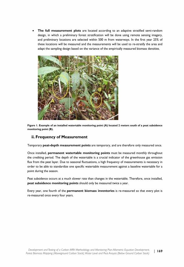
| 169Development and Testing of a Carbon MRV Methodology and Monitoring Plan: Allometric Equation Development, Forest Biomass Mapping (Aboveground Carbon Stock), Water Level and Peat Anaysis (Below Ground Carbon Stock)
• Tdata
Figure 1.monitori
ii. F
Tempora
Once insthe credflux fromorder topoint du
Peat subpeat su
Every yere-measu
The full mdesign, in whand preliminthese locatioadapt the sam
Example of ang point (B).
requency
ary peat-de
stalled, permditing period.m the peat lao be able to sring the seas
bsidence occubsidence m
ear, one fourured once ev
measuremenhich a prelimary location
ons will be mmpling design
an installed w
y of Meas
epth measu
manent wa. The depth ayer. Due to standardize oson.
urs at a mucmonitoring p
rth of the pevery four yea
nt plots areminary forests are selecte
measured andn based on th
watertable mo
suremen
rement po
atertable mof the waterseasonal fluc
one specific w
h slower ratpoints shou
ermanent bars.
e located act stratificatioed within 50d the measurhe variance o
onitoring poin
nt
ints are tem
monitoring prtable is a crctuations, a hwatertable m
te than changld only be m
biomass inv
ccording to aon will be do00 m from wrements will of the empiri
nt (A) located
mporary, and
points mustrucial indicathigh frequencmeasurement
ges in the wameasured twic
ventories is
an adaptive one using re
waterways. Inbe used to rcally measur
d 2 meters so
are therefor
t be measuretor of the grcy of measurt against a ba
atertable. Thce a year.
s re-measure
stratified sememote sensinn the first yere-stratify th
red biomass d
outh of a peat
re only measu
ed monthly treenhouse garements is neaseline water
erefore, onc
ed so that ev
mi-random ng imagery, ear 25% of he area and densities.
subsidence
ured once.
throughout as emission ecessary in rtable for a
ce installed,
very plot is

170 | Annex I: Standard Operation Procedure for Field Measurements
iii. R
Figure 2.
During 2kriging isamples block kramount consistinsimple kconfidenproject iAround with 95%area, a cthe transfrom this
Results o
Semivariogra
2008 and 20s an effectivwere taken
riging.Figure of spatial a
ng of nugget kriging. The mnce level. It is peat area Transect 1 i
% confidenceircle of radiusect. Therefos transect, to
of Previo
am of peat de
009, the peave method ttaking the g2 shows theautocorrelatiand a linear
map indicatescan be obseaccording to
in the south e, due to higus of 15km wore, it is reco ensure opt
us Samp
epths based o
at depth wasto spatially eology into ae semivariancion is preser portion. Ts the areas werved that wo the VCS dof the proje
gh variance owas found to commended ttimal coverag
ling Dept
on two existing
s measured extrapolate account. Simce as a functent. The vahe fitted varwhere the pe
with the currdefinitions (mect area, no of the data. A
have a peat to locate ne
ge of the pro
th Measu
g transects
along two tpeat depth
mple kriging ition of dista
ariogram wariogram was eat depth is rent samplinminimally 50 peat that wa
Around Trandepth of minw transects ject area.
urements
ransects. It measures (
s more effecance and inds modeled used to intminimal a ceg density oncm) at a co
as deeper thnsect 2, in thnimally 50 cmat least 15-3
s
was found t(on the conctive than coicates that awith a mixerpolate samertain value anly a small ponfidence levhan 50 cm whe north of tm around the30 km north
that simple dition that
o-kriging or a significant xed model, mples using at the 95% part of the vel of 95%.
was present the project e center of and south
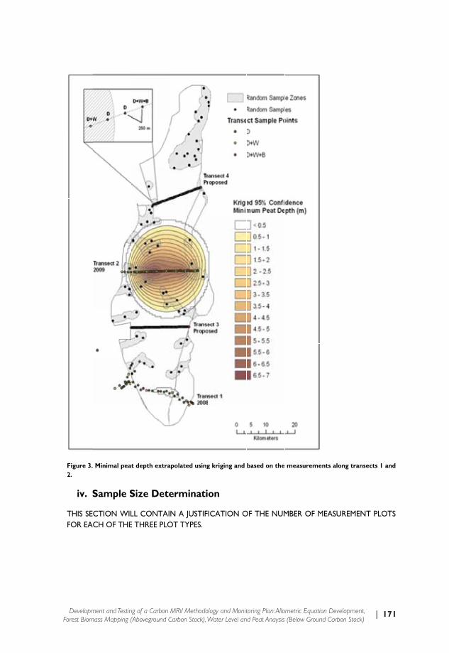
| 171Development and Testing of a Carbon MRV Methodology and Monitoring Plan: Allometric Equation Development, Forest Biomass Mapping (Aboveground Carbon Stock), Water Level and Peat Anaysis (Below Ground Carbon Stock)
Figure 3. 2.
iv. S
THIS SEFOR EA
Minimal peat
Sample S
CTION WILCH OF THE
t depth extra
Size Dete
LL CONTAIE THREE PLO
apolated using
erminati
N A JUSTIFOT TYPES.
g kriging and
on
ICATION O
based on the
OF THE NUM
measuremen
MBER OF M
nts along tran
EASUREMEN
nsects 1 and
NT PLOTS
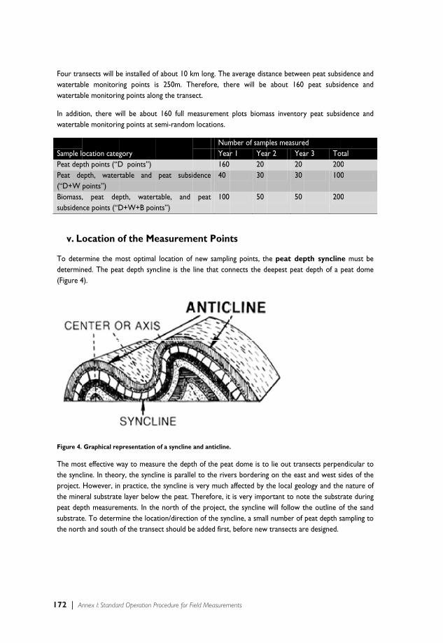
172 | Annex I: Standard Operation Procedure for Field Measurements
Four trawatertabwatertab
In additiwatertab
Sample lPeat depPeat de(“D+W Biomass,subsiden
v. L
To detedetermin(Figure 4
Figure 4.
The mosthe syncproject. the minepeat depsubstratethe nort
nsects will bble monitorible monitorin
ion, there wble monitorin
ocation categpth points (“Depth, waterpoints”) , peat de
nce points (“D
ocation o
rmine the mned. The pea4).
Graphical re
st effective wline. In theoHowever, in
eral substratepth measureme. To determh and south
be installed oing points ing points alo
will be aboutng points at s
goryD points”) rtable and
pth, watertD+W+B poi
of the Me
most optimalat depth syn
presentation
way to measury, the syncl
n practice, the layer belowments. In the
mine the locaof the transe
of about 10 ks 250m. Thng the transe
t 160 full msemi-random
peat subsi
table, and nts”)
easurem
location of ncline is the
of a syncline
ure the deptine is paralle
he syncline isw the peat. Te north of tation/directioect should be
km long. The herefore, theect.
easurement m locations.
NumYear160
dence 40
peat 100
ent Poin
new sampliline that con
and anticline.
th of the peael to the rives very much Therefore, itthe project, ton of the syne added first,
average distere will be
plots bioma
mber of sampr 1 Yea
2030
50
ts
ng points, thnnects the d
.
at dome is toers borderingaffected by t
t is very impothe syncline cline, a smal, before new
tance betweeabout 160
ass inventory
ples measurear 2 Yea
20 30
50
he peat depeepest peat
o lie out trang on the eastthe local geoortant to nowill follow tl number of
w transects ar
en peat subspeat subsi
y peat subsi
ed ar 3 To
200100
200
pth synclindepth of a
nsects perpet and west sology and thete the substrthe outline opeat depth s
re designed.
sidence and dence and
idence and
otal 0 0
0
ne must be peat dome
ndicular to sides of the e nature of rate during of the sand sampling to
| 173Development and Testing of a Carbon MRV Methodology and Monitoring Plan: Allometric Equation Development, Forest Biomass Mapping (Aboveground Carbon Stock), Water Level and Peat Anaysis (Below Ground Carbon Stock)
We recommend to prioritize measuring the peat depth around transect 2 (Figure 5) at different locations that are relatively accessible and at different locations along the north-south axis. Once these peat depths are available, and more information on the geology of the substrate layer is available, the peat depth syncline can be outlined.
After the peat depth syncline is identified, it is recommended to add two east-west transects perpendicular to the peat depth syncline in addition to the two transects that were already measured, one around 17 km south of the most northern transect, and another around 23 km north of the most northern transect. Figure 5 shows an example of the full sampling strategy. The total distance of the four transects combined is ~100 km. A total of 400 points will be located on the four transects after three years, an additional 100 points will be located based on a stratified semi-random sampling scheme. Peat depth will be measured on all 500 locations, while peat subsidence and water monitoring points will only be installed on 60% of the sampling points to yield 300 samples in total. Along the additional transects, biomass will be sampled on 25% of the transect locations, to yield 100 samples in total. In addition, about 100 measurement points on which peat depth, water-table depth, peat subsidence, and biomass stock density will be measured are located on semi-random locations that are easily accessible through canals and in the “low pole” forest cover class.
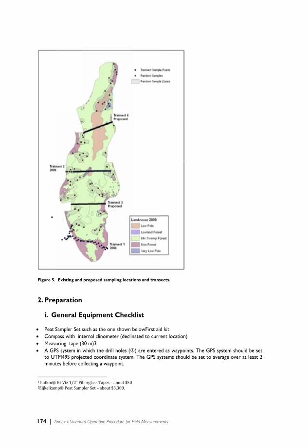
174 | Annex I: Standard Operation Procedure for Field Measurements
Figure 5.
2. Pre
i. G
• Peat S• Comp• Meas• A GP
to UTminut
3 Lufkin®2Eijkelkam
Existing and
paration
General E
Sampler Set pass with inturing tape (
PS system in TM49S projetes before co
® Hi‐Viz 1/2" Fimp® Peat Samp
d proposed sam
n
Equipmen
such as the oternal clinom30 m)3 which the d
ected coordiollecting a wa
iberglass Tapespler Set – abou
mpling locatio
nt Check
one shown bmeter (declin
rill holes (nate system.aypoint.
s – about $50ut $3,300.
ons and trans
klist
belowFirst aidated to curr
) are entere. The GPS sy
sects.
d kit rent location)
ed as waypoiystems shoul
)
nts. The GPld be set to
S system shoaverage over
ould be set r at least 2

| 175Development and Testing of a Carbon MRV Methodology and Monitoring Plan: Allometric Equation Development, Forest Biomass Mapping (Aboveground Carbon Stock), Water Level and Peat Anaysis (Below Ground Carbon Stock)
• Digita• Extra• Mach• Two-• Maps• Satell• Samp• Data • Clipb• Calip• Plasti• Scales• PVC
ii. AB
The mea
field cat leaat leaperm
It is veryquality otechniquand resp
al camera a batteries foete -way radio showing theite Phone
ple container/sheet
board ers c rope s/balance pipe cutter
ArrangemBiomass I
asurement pl
crew leader ast 2 survey aast 2 local anent measu
y important tof the measuues, and safetponsibilities d
r all electron
e plots and lo
/bag
ment of nventori
ots will be in
assistants helcrew-membe
uring points.
that each fieldurements, anty issues. All
during the me
nic instrumen
ocation of th
Work es
nstalled by a
lping the fielders who he
d crew be thnd the safetyl field crew easurement.
nts (at least 8
e sampling p
for Sam
field crew w
d crew leadelps by blazin
horoughly tray of the cremembers neIn general, t
8 batteries).
oints for eac
mpling P
which consists
er ng trails wit
ained before ew. The traineed to have he responsib
ch of the four
Point In
s of:
th the mach
going out inning should a clear unde
bilities are as
r component
nstallatio
hete, and ins
the field to cover auger
erstanding offollows:
ts.
on, and
stalling the
ensure the r operating f their role
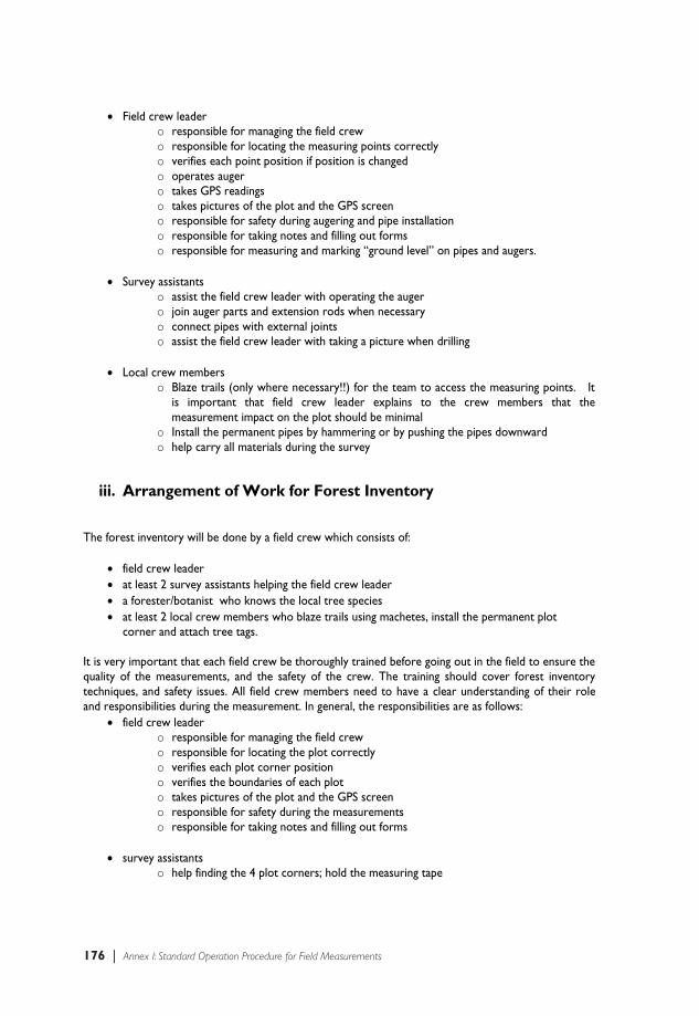
176 | Annex I: Standard Operation Procedure for Field Measurements
• Field crew leader o responsible for managing the field crew o responsible for locating the measuring points correctly o verifies each point position if position is changed o operates auger o takes GPS readings o takes pictures of the plot and the GPS screen o responsible for safety during augering and pipe installation o responsible for taking notes and filling out forms o responsible for measuring and marking “ground level” on pipes and augers.
• Survey assistants o assist the field crew leader with operating the auger o join auger parts and extension rods when necessary o connect pipes with external joints o assist the field crew leader with taking a picture when drilling
• Local crew members o Blaze trails (only where necessary!!) for the team to access the measuring points. It
is important that field crew leader explains to the crew members that the measurement impact on the plot should be minimal
o Install the permanent pipes by hammering or by pushing the pipes downward o help carry all materials during the survey
iii. Arrangement of Work for Forest Inventory
The forest inventory will be done by a field crew which consists of:
• field crew leader • at least 2 survey assistants helping the field crew leader • a forester/botanist who knows the local tree species • at least 2 local crew members who blaze trails using machetes, install the permanent plot
corner and attach tree tags.
It is very important that each field crew be thoroughly trained before going out in the field to ensure the quality of the measurements, and the safety of the crew. The training should cover forest inventory techniques, and safety issues. All field crew members need to have a clear understanding of their role and responsibilities during the measurement. In general, the responsibilities are as follows:
• field crew leader o responsible for managing the field crew o responsible for locating the plot correctly o verifies each plot corner position o verifies the boundaries of each plot o takes pictures of the plot and the GPS screen o responsible for safety during the measurements o responsible for taking notes and filling out forms
• survey assistants
o help finding the 4 plot corners; hold the measuring tape

| 177Development and Testing of a Carbon MRV Methodology and Monitoring Plan: Allometric Equation Development, Forest Biomass Mapping (Aboveground Carbon Stock), Water Level and Peat Anaysis (Below Ground Carbon Stock)
o delineate the plot boundaries with rope as instructed by the field crew leader o measure the trees and call the measurements, to be recorded by the team leader o help carry all materials
• local crew members
o Blaze trails (only where necessary!!) for the team to access the plot boundaries. It is important that field crew leader explains to the local crews that the measurement impact on the plot should be minimal
o Tag the trees as instructed by the team leader and assistants o Install the permanent plot markers at corners o help carry all materials
After the training, the field crew is ready to measure plots. This consists of:
• locating the sample plot (Section 3.f.iii) • measurements in sample plot (Sections 11-3.f.xi)
Before the field work, each team member must be aware of where 1.3 m above the ground level is located on his/her body for DBH measurements. This must be done by exactly measuring 1.3 m for each crew member or just bring the wooden stick with 1.3 length.
iv. Estimated Rime Required for each of the Procedures
Carbon Pool to be Sampled Estimated Time NeededNested Plot boundary demarcation 60 minutes Measuring live trees within the 10x10 m plot 15 minutes Measuring live trees within the 20x20 m plot 15 minutes Measuring standing dead wood 15 minutesMeasuring lying dead wood 15 minutesMeasuring peat depth 30 minutesInstalling water-table tube 10 minutes Installing peat subsidence tube 30 minutes TOTAL 3 hours 10 min
3. Procedures
a. Measurement of Peat Depth
i. Equipment Checklist
• Peat Sampler Set: Spearhead, extension rods and handle4. • Survey data from previous years. • “Measurement of Peat Depth” data sheet. • protective hand gloves • Sample container/bags
4 An example of a Peat Sampler Set can be found at: http://eijkelkamp.com/files/media/Gebruiksaanwijzingen/EN/m1‐0409epeatsamplerset.pdf
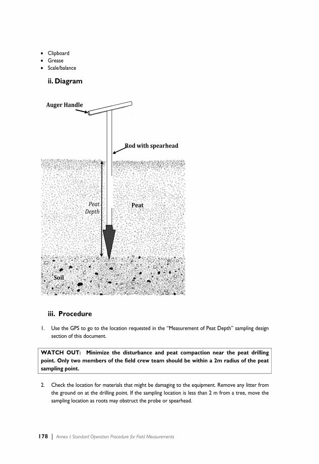
178 | Annex I: Standard Operation Procedure for Field Measurements
• Clipb• Greas• Scale/
ii. D
iii. P
1. Usesect
WATCpoint. Osamplin 2. Che
the sam
So
Auge
board se /balance
Diagram
Procedur
e the GPS totion of this d
CH OUT: Only two mng point.
eck the locatground on a
mpling locatio
oil
erHandle
D
re
o go to the lodocument.
Minimize tmembers of
tion for mateat the drilling
on as roots m
PeatDepth
ocation requ
the disturbf the field c
erials that mig point. If th
may obstruct
Pea
Rodw
ested in the
bance and crew team
ight be damahe sampling lothe probe o
at
withspearh
“Measureme
peat compshould be
aging to the eocation is lesr spearhead.
head
ent of Peat D
paction newithin a 2m
equipment. Rss than 2 m
Depth” samp
ear the peam radius of
Remove any from a tree,
pling design
at drilling f the peat
litter from , move the
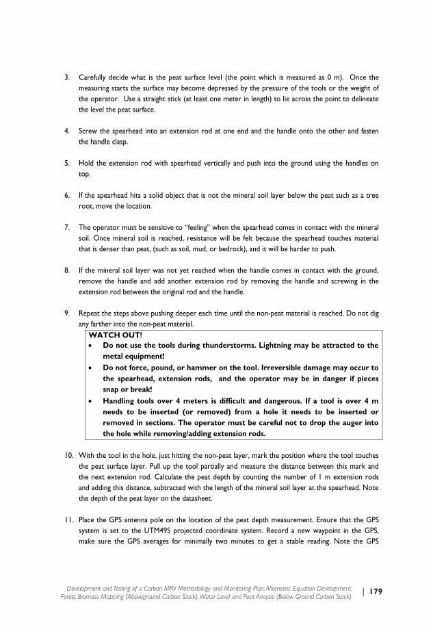
| 179Development and Testing of a Carbon MRV Methodology and Monitoring Plan: Allometric Equation Development, Forest Biomass Mapping (Aboveground Carbon Stock), Water Level and Peat Anaysis (Below Ground Carbon Stock)
3. Carefully decide what is the peat surface level (the point which is measured as 0 m). Once the
measuring starts the surface may become depressed by the pressure of the tools or the weight of the operator. Use a straight stick (at least one meter in length) to lie across the point to delineate the level the peat surface.
4. Screw the spearhead into an extension rod at one end and the handle onto the other and fasten
the handle clasp. 5. Hold the extension rod with spearhead vertically and push into the ground using the handles on
top. 6. If the spearhead hits a solid object that is not the mineral soil layer below the peat such as a tree
root, move the location. 7. The operator must be sensitive to “feeling” when the spearhead comes in contact with the mineral
soil. Once mineral soil is reached, resistance will be felt because the spearhead touches material that is denser than peat, (such as soil, mud, or bedrock), and it will be harder to push.
8. If the mineral soil layer was not yet reached when the handle comes in contact with the ground,
remove the handle and add another extension rod by removing the handle and screwing in the extension rod between the original rod and the handle.
9. Repeat the steps above pushing deeper each time until the non-peat material is reached. Do not dig
any farther into the non-peat material. WATCH OUT! • Do not use the tools during thunderstorms. Lightning may be attracted to the
metal equipment! • Do not force, pound, or hammer on the tool. Irreversible damage may occur to
the spearhead, extension rods, and the operator may be in danger if pieces snap or break!
• Handling tools over 4 meters is difficult and dangerous. If a tool is over 4 m needs to be inserted (or removed) from a hole it needs to be inserted or removed in sections. The operator must be careful not to drop the auger into the hole while removing/adding extension rods.
10. With the tool in the hole, just hitting the non-peat layer, mark the position where the tool touches
the peat surface layer. Pull up the tool partially and measure the distance between this mark and the next extension rod. Calculate the peat depth by counting the number of 1 m extension rods and adding this distance, subtracted with the length of the mineral soil layer at the spearhead. Note the depth of the peat layer on the datasheet.
11. Place the GPS antenna pole on the location of the peat depth measurement. Ensure that the GPS
system is set to the UTM49S projected coordinate system. Record a new waypoint in the GPS, make sure the GPS averages for minimally two minutes to get a stable reading. Note the GPS
180 | Annex I: Standard Operation Procedure for Field Measurements
coordinate and the ID of the waypoint in the “Measurement of Peat Depth” data sheet and take a picture of the GPS screen showing the location with the digital camera. Note down the photo file ID on the datasheet. If possible, take reading from two GPSs, and compare the results. If the readings have less than a 5 meter difference, the readings are acceptable. If the readings are more than 5 meters apart hold the GPSs much higher above the hole, and try to hold back any vegetation that maybe inhibiting any satellite reception.
12. Stand over the point and take a picture in each of the north, south, east, west directions. Note
down the four photo file IDs in the datasheet. Fill out the other required information on the field datasheet.
13. In addition to a central measuring with a peat measuring tool, the peat depth must be checked by
inserting a “stick” in the peat at five locations within 25-m around the central auger point. The measuring stick can be made with the same materials as the pipes for boring.
14. Draw a picture of the area around the point to help identify the point for future measurements.
Include a description of the soil surface and vegetation present. 15. Conduct two more peat dept measurements by only following steps1-10. The two additional
measurements are located within 2 meters of the sampling point. The three samples will be averaged to measure the peat depth.
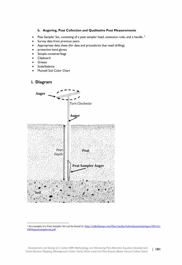
| 181Development and Testing of a Carbon MRV Methodology and Monitoring Plan: Allometric Equation Development, Forest Biomass Mapping (Aboveground Carbon Stock), Water Level and Peat Anaysis (Below Ground Carbon Stock)
b
• P• S• A• p• S• C• G• S• M
i. D
5 An exam0409epea
So
A
Figure 6
b. Augerin
Peat SamplerSurvey data fAppropriate protective haSample contaClipboard Grease Scale/balanceMunsell Soil
Diagram
mple of a Peat Satsamplerset.pd
oil
Auger
.Auger with Pe
ng, Peat Co
r Set, consistfrom previoudata sheet (f
and gloves ainer/bags
e Color Chart
ampler Set candf
PeatDepth
at Sampler Aug
ollection an
ting of a peatus years. for data and
t
n be found at: h
Pe
PeatSam
Auger
TurnClockw
ger Head
nd Qualitati
t sampler hea
procedures
http://eijkelkam
eat
mplerAuge
wise
ive Peat Me
ad, extension
that need dr
mp.com/files/
er
easuremen
n rods, and a
rilling).
media/Gebrui
nts
a handle. 5
ksaanwijzingen/EN/m1‐

182 | Annex I: Standard Operation Procedure for Field Measurements
ii. Procedure
1. Use the GPS to go to the location requested in the appropriate datasheet.
WATCH OUT: Minimize the disturbance and peat compaction near the peat drilling point. Only two field crew team members should be within a 2m radius of the peat drilling point.
2. Check the auguring location for materials that might be damaging to the auguring equipment. Remove any litter from the ground on at the drilling point. If the sampling location is less than 2 m from a tree, move the sampling location as roots may obstruct the auger.
3. Carefully decide what is the peat surface level (the point which is measured as 0 m). Once auguring starts the surface may become depressed by the pressure of the auger or the weight of the operator. Use a straight stick (at least one meter in length) to lie across the point to delineate the level the peat surface.
4. Screw the auger head into an extension rod at one end and the handle onto the other and fasten the handle clasp.
5. Ensure the blade at the auger’s head is properly closed. Hold the auger vertically and push the auger 10 cm in the ground using the handles on top.
6. If the auger hits a solid object, such as rocks in the soil, bedrock, or a tree root, move the location.
7. Gradually push the auger downward into the peat layer for a maximum of 1 meter. While pushing the auger downward, do not rotate the auger.
8. After pushing the auger for 1 meter, rotate the handle of auger clockwise 360⁰ to take the peat sample. Rotating the handle 360⁰ clockwise is intended to open the blade and to insert the peat soil into the auger head.
WATCH OUT: Always turn the auger clockwise, turning it counterclockwise can damage the auger! Before drilling, always check that the blade of the auger is closed properly.
9. Carefully pull the auger out of the hole so that the peat sample remains inside the auger head.
10. Open the blade carefully and inspect whether mineral soil is present within the sample. If mineral soil is present, continue with step 13.
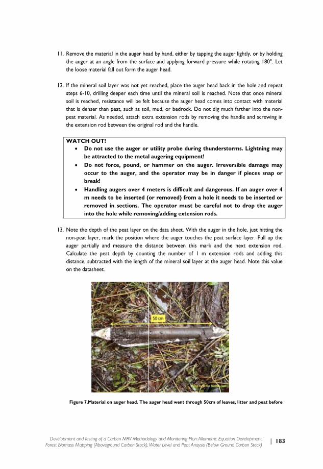
| 183Development and Testing of a Carbon MRV Methodology and Monitoring Plan: Allometric Equation Development, Forest Biomass Mapping (Aboveground Carbon Stock), Water Level and Peat Anaysis (Below Ground Carbon Stock)
11. Rtt
12. Isstpt W
13. N
naCdo
Remove the the auger at the loose ma
If the minerasteps 6-10, dsoil is reachethat is densepeat materiathe extensio
WATCH O• Do
be a• Do
occubrea
• Hanm nreminto
Note the denon-peat layauger partiaCalculate thdistance, subon the datash
Figure 7.Ma
material in tan angle fro
aterial fall ou
al soil layer wdrilling deepeed, resistancer than peat,al. As neededn rod betwe
OUT! not use the
attracted tonot force, ur to the aak! ndling augeneeds to be
moved in seo the hole w
epth of the pyer, mark thelly and meae peat dept
btracted withheet.
aterial on auge
the auger heaom the surfat form the au
was not yet er each timee will be felt such as soild, attach exten the origin
e auger or o the metal
pound, orauger, and
rs over 4 me inserted (ections. Thwhile remov
eat layer on e position wasure the dith by counth the length
er head. The
ad by hand, eace and applyuger head.
reached, plae until the mt because thel, mud, or betra extensionnal rod and t
utility prol augering er hammer
the opera
meters is dor removee operatorving/adding
the data shewhere the aug
istance betwting the numof the miner
auger head w
either by tapying forward
ace the augermineral soil ise auger headedrock. Do nn rods by rehe handle.
be during tequipment!on the au
ator may b
ifficult anded) from a hr must be g extension
eet. With thger touches
ween this mmber of 1 mral soil layer
went through
ping the auged pressure w
r head back s reached. Nd comes intonot dig muchmoving the h
thundersto! ger. Irreve
be in dange
dangeroushole it neecareful notrods.
e auger in ththe peat sur
mark and them extension
at the auger
50cm of leave
er lightly, or while rotating
in the hole Note that ono contact with farther inthandle and s
orms. Light
ersible damer if pieces
s. If an augds to be int to drop t
he hole, just rface layer. Pe next exte
rods and ar head. Note
es, litter and
by holding g 180°. Let
and repeat nce mineral th material o the non-screwing in
tning may
mage may s snap or
ger over 4 serted or the auger
hitting the Pull up the nsion rod. adding this e this value
peat before

184 | Annex I: Standard Operation Procedure for Field Measurements
14. Dhdr
15. ICw
hitting the h
Draw a skethead(s), and depth. In thright side. No
Identify the Color Chartwritten as H
Peat dept vegetationspongy, aPeat color
Mun
Hue:
Value:
Chroma
hard soil layer
tch of the soadding them
e diagram prote unique fe
color of thet. Record thue Value/Ch
was 29.5 cn is thick fand coveredr was 7.5YR
nsell ColorPeaColo
7.5YR
4/ a: /6
r.
oil profile likm up to extrrovided the aeatures in th
e soil (at thee hue, valueroma. The st
m. There waforest. Manyd in leaves. R 4/6, and
r Chart Coat or
Soi
R 5 Y
5/
/8
ke the one rapolate a soauger end is e soil profile
e bottom of e and chromatared examp
as about 8.5y large kep soil color w
olor il Color
YR
5/
8
below by exoil profile. Beon the left s
e, and write a
the auger) aa on the as
ple in the ima
5 cm of dufong hantu
was 5 YR 5/
xamining thee sure to wside, while tha description
and peat by shown belo
age below is w
ff, litter an trees presen
5/8.
e material inrite down cm
he soil surfac on the sketc
using the Mw. Soil colowritten as “1
nd leaves. Thnt. Surface
the auger m to mark
ce is on the ch sheet.
Munsell Soil r is always 10R 4/2”.
he is wet,

| 185Development and Testing of a Carbon MRV Methodology and Monitoring Plan: Allometric Equation Development, Forest Biomass Mapping (Aboveground Carbon Stock), Water Level and Peat Anaysis (Below Ground Carbon Stock)
c
This sectcolor and“Sketch,
1. Strat
2. Colle
3. Recobe ta
4. Use base
5. For dept
6. The
7. Turnsamp
8. Collecylindistuno.,
c. Measur
ion must follod soil color, vegDescription a
tify the entire
ect at least t
ord Strata naaken. Use da
the peat same “bottom” o
each sample th at which it
sampler is o
n the sampleple to be col
ect the samndrical enclourbance wheand depth fr
Figure 8. Mun
ement of C
ow the augurgetation around Sample Co
e area with p
two cores pe
ame, core id,atasheet “Ske
mpler head tof the peat.
assign a Cot was extract
operated by m
er clockwise lected.
mple and transure of knore it will be
rom where th
sell Soil Color C
Carbon Con
ring instructionnd the point, ollection”, the
peat accordin
er stratum. It
, field crew, detch, Descrip
to collect pe
re ID, recordted.
manually inse
to insert in
nsfer the samown weight, frozen until
he core was
Chart is used to
ntent of Pea
ns in section and a sketch sample sectio
ng to vegetat
t is advised to
date and GPSption, and Sam
eat core sam
d the Color
erting the bot
nto the peat
mple cores transport tfurther analyextracted.
Valo keep soil color
at
15. Also recoof the peat p
on must be fil
tion type and
o collect mul
S location ofmple Collect
mples in 50 c
using the M
ttom point o
and turn sa
into a suitabhese sampleyzed. Label e
uers standard.
ord qualitativeprofile. This selled out.
d/or land cov
ltiple cores, i
f the point frtion”.
m increment
unsell Color
of the sample
ampler count
ble containees to the labeach core wi
e measuremeection uses th
ver.
if resources
rom where sa
ts from the
r Chart, and
er into the pe
ter clockwis
er such as a boratory witith stratum n
H
Chro
ents of peat e datasheet
permit.
ample is to
top to the
record the
eat.
se to allow
polythene th minimal name, core
Hu
oma
186 | Annex I: Standard Operation Procedure for Field Measurements
9. Enter date on which samples were sent to lab and name of lab.
10. Follow any additional procedures provided by the laboratory in order to analyze carbon content and
soil moisture content. The moisture content will most likely be determined at the laboratory and can be obtained by oven drying the sample at 70C using standard procedures. Use standard C analysis procedures to estimate the carbon content in the sample. Various methods are available such as flash combustion (Carlo Erba Analyzers, CHN Analyzers, …) or wet oxidation (Walkey and Black). Any method for C analysis is allowed on the condition that the analysis is sufficiently calibrated and all required QA/QC procedures are executed.
11. Record the carbon content and moisture content of each core in the “peatcore” worksheet of the excel workbook.
12. Record the lab report date, the contact details of the lab supervisor and the cost per sample for future reference.
13. Repeat step 2 to 12 for other cores and other strata.
d. Installation of Permanent Watertable Monitoring Point
This section must follow the auguring instructions in section 15. Also record qualitative measurements of peat color and soil color, vegetation around the point, and a sketch of the peat profile. This section uses the datasheets “Peat Watertable and Subsidence” and “Sketch, Description and Sample Collection”, the sample section is not filled out if a sample is not needed.
i. Equipment Checklist
• Peat Sampler Set, consisting of an Edelman auger head, extension rods, and a handle.6 • Survey data from previous years. • 5-cm or 2.5 inch diameter perforated PVC tubes cut to 1 m length. • Solid rubber lids or plastic caps to close the PVC tubes • “Watertable Monitoring Point” data sheet • Measurement stick • Hammer or Mallet • PVC pipe cutter • Digital camera
If automatic samplers are used the following extra equipment must be brought to the field:
• HOBO U20 Water Level Data Logger - U20-001-017 • Optic USB Base Station - BASE-U-48
6 An example of all equipment needed for peat augering can be found in the Eijelkamp Peat Sampler Set. http://eijkelkamp.com/files/media/Gebruiksaanwijzingen/EN/m1‐0409epeatsamplerset.pdf 7 http://www.onsetcomp.com/products/data‐loggers/u20‐001‐01 8 http://www.onsetcomp.com/products/communications/base‐u‐4
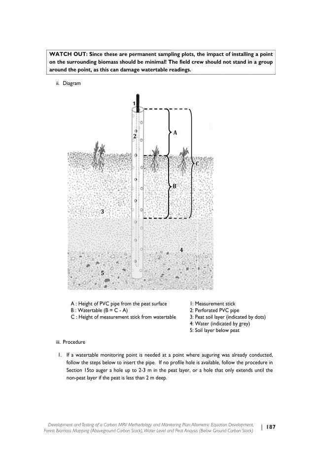
| 187Development and Testing of a Carbon MRV Methodology and Monitoring Plan: Allometric Equation Development, Forest Biomass Mapping (Aboveground Carbon Stock), Water Level and Peat Anaysis (Below Ground Carbon Stock)
WATCon the saround
ii. D
iii. Pr
1. IfSn
CH OUT: Sisurroundinthe point,
iagram
A : Height B : WatertC : Height
rocedure
If a watertabfollow the stSection 15tonon-peat laye
Figu
ince these ng biomass as this can
of PVC pipetable (B = C of measurem
ble monitoriteps below too auger a hoer if the peat
3
5
re 9.Permanen
are permashould be mdamage w
e from the pe- A)
ment stick fro
ng point is no insert the le up to 2-3t is less than
2
1
nt Watertable M
nent sampminimal! Tatertable r
eat surface
om watertab
needed at a pipe. If no p m in the pe2 m deep.
Monitoring Poin
ling plots, tThe field crereadings.
ble
1: M2: P3: P4: W5: S
point whereprofile hole ieat layer, or
B
4
A
C
nt
the impactew should n
MeasurementPerforated PVPeat soil layerWater (indicaoil layer belo
e auguring ws available, fo
r a hole that
C
t of installinnot stand in
t stick VC pipe r (indicated bated by grey)ow peat
was already collow the pronly extend
ng a point n a group
by dots) )
conducted, rocedure in ds until the
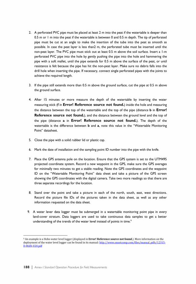
188 | Annex I: Standard Operation Procedure for Field Measurements
2. A perforated PVC pipe must be placed at least 2 m into the peat if the watertable is deeper than 0.5 m or 1 m into the peat if the watertable is between 0 and 0.5 m depth. The tip of perforated pipe must be cut at an angle to make the insertion of the tube into the peat as smooth as possible. In case the peat layer is less than2 m, the perforated tube must be inserted until the non-peat layer. The PVC pipe must stick out at least 0.5 m above the soil surface. Insert a 1-m perforated PVC pipe into the hole by gently pushing the pipe into the hole and hammering the pipe with a soft mallet, until the pipe extends for 0.5 m above the surface of the peat, or until resistance is felt because the pipe has hit the non-peat layer. Make sure no debris falls into the drill hole when inserting the pipe. If necessary, connect single perforated pipes with the joints to achieve the required length.
3. If the pipe still extends more than 0.5 m above the ground surface, cut the pipe at 0.5 m above the ground surface.
4. After 15 minutes or more measure the depth of the watertable by inserting the water measuring stick (f in Error! Reference source not found.) inside the hole and measuring
the distance between the top of the watertable and the top of the pipe (distance b in Error! Reference source not found.), and the distance between the ground level and the top of
the pipe (distance a in Error! Reference source not found.). The depth of the watertable is the difference between b and a, note this value in the “Watertable Monitoring Point” datasheet.
5. Close the pipe with a solid rubber lid or plastic cap.
6. Mark the date of installation and the sampling point ID number into the pipe with the knife.
7. Place the GPS antenna pole on the location. Ensure that the GPS system is set to the UTM49S projected coordinate system. Record a new waypoint in the GPS, make sure the GPS averages for minimally two minutes to get a stable reading. Note the GPS coordinates and the waypoint ID on the “Watertable Monitoring Point” data sheet and take a picture of the GPS screen showing the GPS coordinates with the digital camera. Take two more readings so that there are three separate recordings for the location.
8. Stand over the point and take a picture in each of the north, south, east, west directions. Record the picture file IDs of the pictures taken in the data sheet, as well as any other information requested on the data sheet.
9. A water lever data logger must be submerged in a watertable monitoring point pipe in every land-cover stratum. Data loggers are used to take continuous data samples to get a better understanding of the trends of the water level instead of points in time.9
9 An example is a Hobo water level logger (displayed in Error!Referencesourcenotfound.). More information on the deployment of the water level logger can be found in its manual: http://www.onsetcomp.com/files/manual_pdfs/12315‐D‐MAN‐U20.pdf

| 189Development and Testing of a Carbon MRV Methodology and Monitoring Plan: Allometric Equation Development, Forest Biomass Mapping (Aboveground Carbon Stock), Water Level and Peat Anaysis (Below Ground Carbon Stock)
e
This sectcolor anddatasheenot filled
i. Eq
• P•
poR
• “• K• H• B• P• D• D
e. Installat
ion must follod soil color, ts “Peat Depout if a samp
quipment Ch
Peat Sampler1-m length, permanent sof pipes and Reference“Peat SubsideKnife and peHammer or Bags of cemePipe connectDevice to poDigital camer
Fig
tion of Pea
ow the augurvegetation arth Measurem
ple is not need
ecklist
r Set, consist5-cm (or 2
ubsidence hojoints taken
e source noence Monitormanent marmallet ent to fill thetor/joints our cement inra
ure 10.Hobo w
at Subsidenc
ring instructionround the po
ment” and “Skded.
ting of an Ede2-cm) diameoles and exten to the fieldot found. boring” data shrker to mark
e full-length P
nto the pipe
water-level logge
ce Monitor
ns in section oint, and a sketch, Descrip
elman auger eter non-perernal pipe joid must be eqbelow. heet k subsidence
PVC tube. Th
(corong in In
er and deploym
ring Points
15. Also recosketch of theption and Sam
head, extensrforated PVints to connequivalent wit
tubes.
he quantity o
ndonesian)
ment diagram.
ord qualitativee peat profilemple Collection
sion rods, anC pipes to ect the pipesth the full pe
f cement wil
e measuremee. This section”, the samp
d a handle. be inserted
in the field. eat depth. S
l vary with p
ents of peat on uses the le section is
d into the The length ee Error!
peat depth.
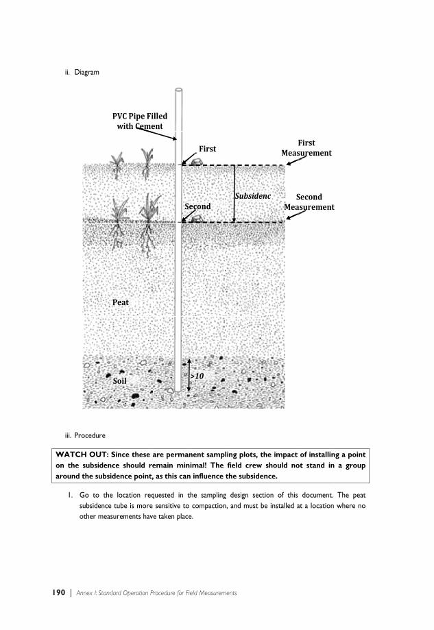
190 | Annex I: Standard Operation Procedure for Field Measurements
ii. D
iii. Pr
WATCon the around
1. Gso
iagram
rocedure
CH OUT: Sisubsidencethe subside
Go to the subsidence tother measu
P
P
S
Figure 1
ince these e should reence point,
location reqtube is morerements hav
PVCPipeFiwithCeme
Peat
Soil
11.Permanent P
are permaemain min, as this can
quested in t sensitive to
ve taken place
illedent
S
Peat Subsidence
nent sampnimal! The n influence
the samplingo compactione.
>10
First
econd
e Sampling Plot
ling plots, tfield crewthe subside
g design secn, and must b
Subside
t
the impactw should noence.
ction of thisbe installed a
Meas
SMea
enc
t of installinot stand in
s document. at a location
Firstsurement
Secondasurement
ng a point n a group
The peat n where no
t
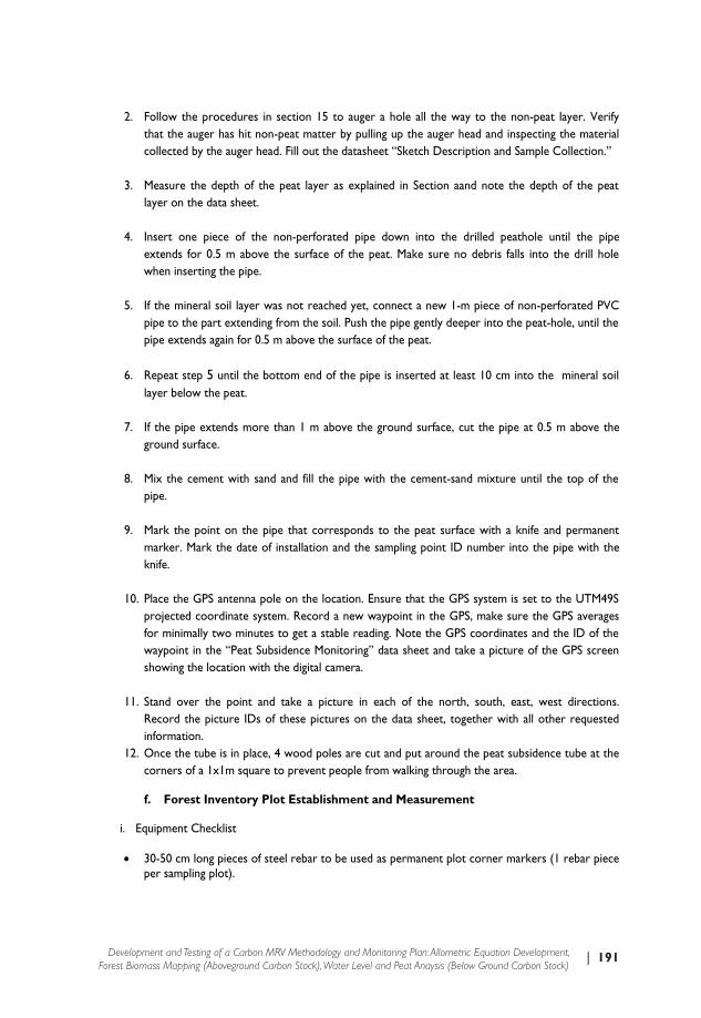
| 191Development and Testing of a Carbon MRV Methodology and Monitoring Plan: Allometric Equation Development, Forest Biomass Mapping (Aboveground Carbon Stock), Water Level and Peat Anaysis (Below Ground Carbon Stock)
2. Follow the procedures in section 15 to auger a hole all the way to the non-peat layer. Verify that the auger has hit non-peat matter by pulling up the auger head and inspecting the material collected by the auger head. Fill out the datasheet “Sketch Description and Sample Collection.”
3. Measure the depth of the peat layer as explained in Section aand note the depth of the peat layer on the data sheet.
4. Insert one piece of the non-perforated pipe down into the drilled peathole until the pipe extends for 0.5 m above the surface of the peat. Make sure no debris falls into the drill hole when inserting the pipe.
5. If the mineral soil layer was not reached yet, connect a new 1-m piece of non-perforated PVC pipe to the part extending from the soil. Push the pipe gently deeper into the peat-hole, until the pipe extends again for 0.5 m above the surface of the peat.
6. Repeat step 5 until the bottom end of the pipe is inserted at least 10 cm into the mineral soil layer below the peat.
7. If the pipe extends more than 1 m above the ground surface, cut the pipe at 0.5 m above the ground surface.
8. Mix the cement with sand and fill the pipe with the cement-sand mixture until the top of the pipe.
9. Mark the point on the pipe that corresponds to the peat surface with a knife and permanent marker. Mark the date of installation and the sampling point ID number into the pipe with the knife.
10. Place the GPS antenna pole on the location. Ensure that the GPS system is set to the UTM49S projected coordinate system. Record a new waypoint in the GPS, make sure the GPS averages for minimally two minutes to get a stable reading. Note the GPS coordinates and the ID of the waypoint in the “Peat Subsidence Monitoring” data sheet and take a picture of the GPS screen showing the location with the digital camera.
11. Stand over the point and take a picture in each of the north, south, east, west directions. Record the picture IDs of these pictures on the data sheet, together with all other requested information.
12. Once the tube is in place, 4 wood poles are cut and put around the peat subsidence tube at the corners of a 1x1m square to prevent people from walking through the area.
f. Forest Inventory Plot Establishment and Measurement
i. Equipment Checklist
• 30-50 cm long pieces of steel rebar to be used as permanent plot corner markers (1 rebar piece per sampling plot).

192 | Annex I: Standard Operation Procedure for Field Measurements
• Field equipment to bury the permanent plot markers (shovel or spade) • Temporary plot corner markers • Aluminum nails and numbered tags for marking trees10 • 2 Steel or aluminum metric DBH measuring tapes (no cloth ones)11 • 300 m of flagging rope for temporarily demarcation of plot boundaries • Hatchet (for debarking trees around plot corners) • Data sheet packages
o Measurement plot cover sheet (1 sheet) o Tree biomass sheet (5 sheets) o Dead wood sheet (1 sheet) o Logged tree trunks sheet (1 sheet) o Standing dead sheet (1 sheet)
• Hand clippers and/or pruning saws • Toilet paper to mark plot boundaries, dead wood, and stumps. • Bright colored paint to mark debarked tree faces near plot corners • Clinometer • Six ropes to delineate the plot boundaries and transects. • Maps showing the plots and sampling points • Spherical densiometer for forest canopy measurements • Laser hypsometer for tree height and distance measurements.
10Ben Meadows 152580, 1000 Round Aluminum Tags ‐ $99, Ben Meadows 231631, 1.5 LB BOX, 2‐7/8 inch Aluminum Wood Siding Nails 11 Ben Meadows 97420, Ben Meadows Company 6' Tape Measure ‐ $9.40

| 193Development and Testing of a Carbon MRV Methodology and Monitoring Plan: Allometric Equation Development, Forest Biomass Mapping (Aboveground Carbon Stock), Water Level and Peat Anaysis (Below Ground Carbon Stock)
ii. O
The plot
This proall trees cm are o
iii. Pr
WATCcoordin
10
verview of th
measurement
ocedure useswith a DBH
only measure
rocedures fo
CH OUT: Dnate system
he Forest Inv
ts are obtaine
nested plotgreater than
ed in a 10 X
r Establishing
Double chem, and not t
Measure dalong two
The folthe 20
•
•
••
1
Within10 m pmeasurwith a than 15greaterequal t
ventory Plot
ed within the b
s to reduce n 15 cm are m10 m plot.
g the Invento
eck that ththe local da
downed dea20 m rope
llowing datx 20 m plotMeasure thcover usindensitomeMeasure evtree with aequal to 5 Dominant Measure trgreater tha
10m
the 10 x lot re trees DBH less 5 cm, but r than or to 5 cm.
boundaries of
the number measured 20
ory Plots
he GPS syatum!
20m
adwood > 1transects
ta is collectet: he forest cag the sphereter very standia DBH greatcm. canopy heirees with a an or equal
f the plot.
of trees mea0 X 20 m plo
stem is se
m
10 cm in dia
ed within
anopy rical
ing dead ter than or
ight DBH l to 15 cm.
asured. Withot. Trees with
et to the U
ameter
hin the 20 Xh a DBH grea
UTM 49S p
X 20 m plot ater than 5
projected
N
20m
Three subsampoints aused fomeasurabovegnon‐trebiomascountinseedlin
mple are r ring round ee s and ng gs

194 | Annex I: Standard Operation Procedure for Field Measurements
1. The given GPS coordinate of point is provided on the map and on the data cover sheet. The field crew leader uses the GPS, maps and a compass to locate this point as accurately as possible. Field crew members help the field crew leader by cutting the forest understory growth where and when absolutely necessary.
WATCH OUT: Since these are permanent sampling plots, the impact of measuring a plot must be minimal. The vegetation should only be cut where it is absolutely necessary!
2. Sometimes it is necessary to re-locate the plot following the procedures below in 2 cases: (1)
the location of the GPS coordinate is not accessible due to inaccessible terrain, presence of roads or water bodies, or (2) the observed land-cover class in the field is different than the required land-cover class because of recently occurring deforestation. Plot relocation should follow these steps:
o The team leader notes down why the point was relocated (e.g., landmine danger, recent deforestation).
o The forester finds a location in the forest system that is similar to the inaccessible forest or similar to the required forest. The new position should be as close as possible to the originally requested location.
o Randomizes the location of the new plot by walking a random number of steps (meters) in the north-south direction AND a random number of steps in the east-west direction. Using the following table to select the two not-yet used random numbers. A positive number in the first column indicates a north direction while a negative number indicates a south direction. Likewise, a positive number in the second column indicates an east direction while a negative number indicates a west direction. Once the row of random numbers is used, cross it off the list. Every row of random numbers may only be used once.

| 195Development and Testing of a Carbon MRV Methodology and Monitoring Plan: Allometric Equation Development, Forest Biomass Mapping (Aboveground Carbon Stock), Water Level and Peat Anaysis (Below Ground Carbon Stock)
North-South Randomized Distance (m) East-West Randomized Distance (m) -107 -1830 178-111 61-110 -6194 171-13 -18262 43 -2 37 -13 -184 -19 -57 53 -96 196 -13 170 122 42 -154 76 96 -98 -199 -197 -82 -197 -6870 37-100 81-50 199-196 -69-134 10833 -76
3. The found location is referred to as point in the overview graph and in this text. It is the southwest corner of the sampling plot. Mark this point with a temporary plot corner marker, record a waypoint of this point in the GPS and note down the correct coordinates on the data sheet. Make sure that the GPS system is set to average at least 2 minutes before collecting a waypoint.
4. Synchronize the GPS and the camera by taking a picture of the GPS screen showing the time in
hours, minutes and seconds. Then take a picture of the screen of the GPS device showing the current position (coordinates) of point . As the GPS and the camera are synchronized the camera and the GPS should be carried by the same person. Set the GPS to track mode to track the following steps.
5. Use the compass to locate the north direction from point to point . If north points to a
direction which is not accessible, follow the procedure in step 1 above for plot relocation.
196 | Annex I: Standard Operation Procedure for Field Measurements
6. Walk 20 m north of point , and put a temporary marker to indicate point . One assistant holds a rope at point while the other assistant walks to point holding the other end of the rope. The rope is laid on the ground between point and delineating the western boundary of the plot.
7. Turn the compass to the east direction and walks 20 m from point to point . The team
leader marks point with a temporary marker, and the assistant places rope on the ground delineating the boundary between points and as described above.
8. Turn the compass to the south direction and walk 20 m from point to point . The field
crew leader marks point with a temporary marker, and the assistant places rope on the ground delineating the boundary between points and as described above.
9. Turn the compass to the west direction and walk 20 m from point to point . The field crew
leader makes sure the distance between point and point is 20 m apart. The assistant places rope on the ground delineating the boundary between points and as described above, and complete a square to form the plot. The plot consists of the area within the rope boundaries.
10. The southwest corner (point ) is a permanent measurement point that will need to be re-
located in the future to measure the plot. The steps below are to be followed to properly mark the permanent point;
a) Remove a square of 10 cm x 10 cm of the bark and cambium layer of 4 trees near point as instructed by the team leader.
b) Paint the debarked square with a bright color. (This way if there is no physical corner point one can line themselves up in the center of the market trees and be very near the point). This does some harm to the trees, but also makes them a little less attractive as they are damaged.
c) Install tree tags at inconspicuous location on these trees to help identify the point in the future, and note them down on the sheet.
11. Pictures are then taken to show forest type and canopy cover. Take photos in the directions
north, east, south, west and one picture up into the sky from point . Pictures are taken showing hand signals for the directions, against the data cover sheet showing the plot number. More specifically:
o One finger indicates that the picture was taken in the north direction.
o Two fingers indicate that the picture was taken in the east direction.
o Three fingers indicate that the picture was taken in the south direction.
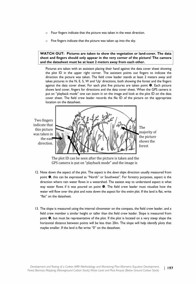
| 197Development and Testing of a Carbon MRV Methodology and Monitoring Plan: Allometric Equation Development, Forest Biomass Mapping (Aboveground Carbon Stock), Water Level and Peat Anaysis (Below Ground Carbon Stock)
Wsa
12. N
pdww“
13. T
fphm
Twoindicthiswas t
di
o Four
o Five
WATCH Osheet and fand the dat
Pictures the plot directiontakes picagainst tshows laput on “cover shlocation
Note down tpoint , thisdirection whway water fwater will flo“flat” on the
The slope is field crew mpoint , buthorizontal dimaybe smalle
o fingerscate thats picturetaken inthe eastirection.
TheGPS
r fingers indic
fingers indica
OUT: Pictufingers shoutasheet mu
are taken wID in the
n the picturectures in the the data covand cover, finplayback mo
heet. The fieon the datas
the aspect os can be exphere rain watflows if it waow over the datasheet.
measured usmember a simt must be reistance betwer. If the land
e plot ID canS camera is
cate that the
ate that the
ures are takuld only ap
ust be at lea
with an assistaupper right
e was taken.N, E, S, W a
ver sheet. Fongers for direode” one caneld crew leadsheet.
f the plot. Tpressed as “Nter flows in aas poured oplot and not
sing the intermilar height opresentative
ween points wd is flat write
n be seen aput on “pla
picture was
picture was t
ken to showppear in theast 2 meter
ant placing thcorner. Th
. The field cand ‘Up’ dire
or each plot ections and t
n zoom in onder records
he aspect is North” or Soa watershed
on point . te down the
rnal clinometor taller than
of the plot. will be less the “0” on the
fter the picayback mod
taken in the
taken up into
w the vegee very cornrs away from
heir hand age assistant prew leader ections, bothfive picture
the data covn the image a
the file ID
the down slopouthwest”. F. The easiestThe field craspect for th
ter on the con the field cr
If the plot ishan 20m. Thdatasheet.
cture is takede” and the
e west direct
o the sky.
etation or laner of the pm each oth
gainst the datpoints out fstands at lea
h showing thes are taken
ver sheet. Wand look at tof the pictu
pe direction For forestry t way to undrew leader mhe entire plot.
ompass, the frew leader. Ss located on he slope will
en and the e image is
Tmtsf
ion.
and-cover. picture! Thher.
ta cover sheefingers to inast 2 meterse forest and point . Ea
When the GPSthe plot ID oure on the a
usually measpurposes, asderstand aspemust visualiz If the land is
field crew leaSlope is meas
a very steephelp identify
The majority of the picture shows the forest
The data e camera
et showing ndicate the s away and the fingers
ach picture S camera is on the data appropriate
sured from spect is the ect is what e how the s flat, write
ader, and a sured from p slope the y plots that
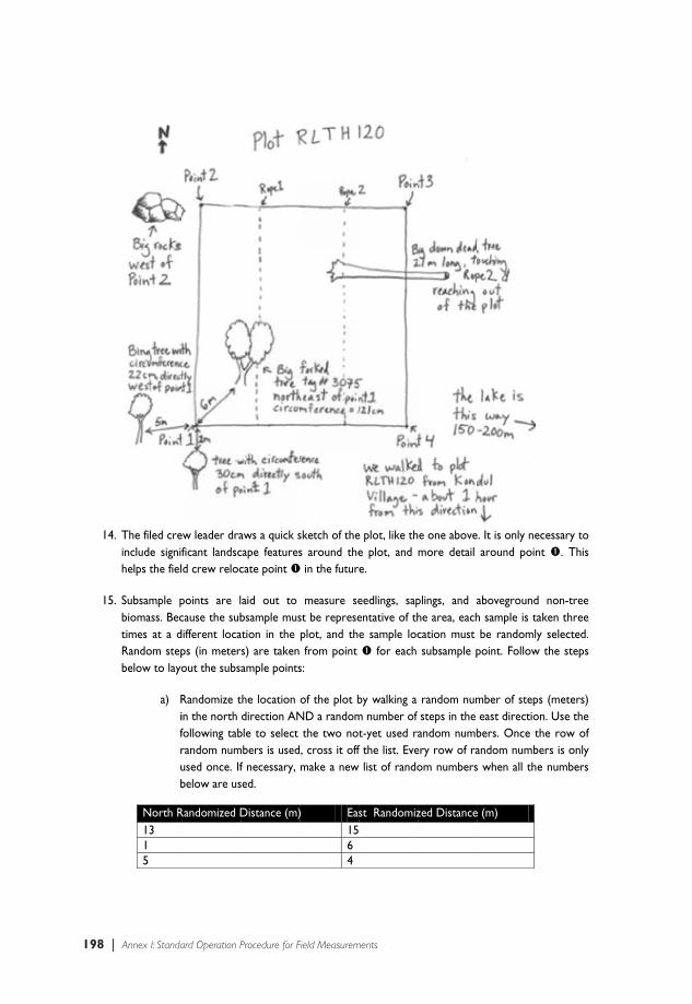
198 | Annex I: Standard Operation Procedure for Field Measurements
14. Tih
15. SbtRb
The filed creinclude signifhelps the fiel
Subsample pbiomass. Bectimes at a dRandom stepbelow to layo
a) Rifrub
North R13 1 5
ew leader draficant landscd crew reloc
points are lcause the subdifferent locaps (in meterout the subs
Randomize tin the north following tabrandom numused once. Ifbelow are us
Randomized D
aws a quick scape featurescate point
aid out to bsample musation in the rs) are takenample points
the location direction AN
ble to select mbers is usedf necessary, sed.
Distance (m)
sketch of thes around the in the futur
measure sest be represeplot, and th from point s:
of the plot bND a random
the two not, cross it offmake a new
) Eas1564
e plot, like the plot, and e.
eedlings, sapentative of the sample loc
for each
by walking a m number of t-yet used raf the list. Eve list of rando
st Randomiz
e one abovemore detail
plings, and ahe area, eachcation must subsample p
random numsteps in the andom numb
ery row of raom numbers
zed Distance
e. It is only nearound poin
abovegroundh sample is tbe randoml
point. Follow
mber of stepeast directio
bers. Once tandom numbs when all th
e (m)
ecessary to nt . This
d non-tree taken three y selected.
w the steps
ps (meters) on. Use the the row of bers is only e numbers
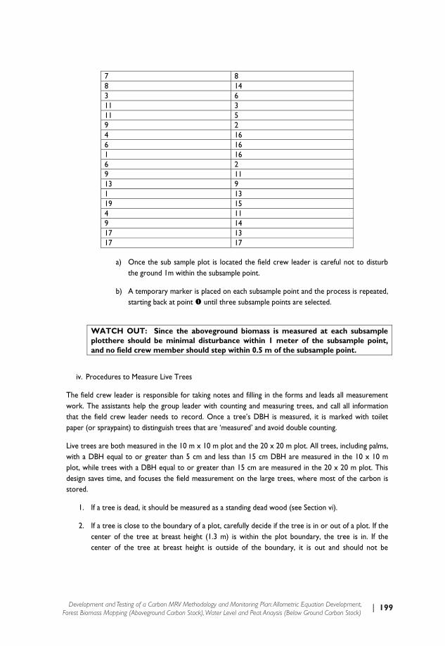
| 199Development and Testing of a Carbon MRV Methodology and Monitoring Plan: Allometric Equation Development, Forest Biomass Mapping (Aboveground Carbon Stock), Water Level and Peat Anaysis (Below Ground Carbon Stock)
7 88 143 611 311 5 9 2 4 16 6 161 16 6 29 1113 91 1319 154 119 1417 13 17 17
a) Once the sub sample plot is located the field crew leader is careful not to disturb
the ground 1m within the subsample point.
b) A temporary marker is placed on each subsample point and the process is repeated, starting back at point until three subsample points are selected.
WATCH OUT: Since the aboveground biomass is measured at each subsample plotthere should be minimal disturbance within 1 meter of the subsample point, and no field crew member should step within 0.5 m of the subsample point.
iv. Procedures to Measure Live Trees
The field crew leader is responsible for taking notes and filling in the forms and leads all measurement work. The assistants help the group leader with counting and measuring trees, and call all information that the field crew leader needs to record. Once a tree’s DBH is measured, it is marked with toilet paper (or spraypaint) to distinguish trees that are ‘measured’ and avoid double counting.
Live trees are both measured in the 10 m x 10 m plot and the 20 x 20 m plot. All trees, including palms, with a DBH equal to or greater than 5 cm and less than 15 cm DBH are measured in the 10 x 10 m plot, while trees with a DBH equal to or greater than 15 cm are measured in the 20 x 20 m plot. This design saves time, and focuses the field measurement on the large trees, where most of the carbon is stored.
1. If a tree is dead, it should be measured as a standing dead wood (see Section vi).
2. If a tree is close to the boundary of a plot, carefully decide if the tree is in or out of a plot. If the center of the tree at breast height (1.3 m) is within the plot boundary, the tree is in. If the center of the tree at breast height is outside of the boundary, it is out and should not be

200 | Annex I: Standard Operation Procedure for Field Measurements
measured. If the tree is exactly on the border of the plot, flip a coin to determine if it is in or out.
3. Ideally each tree is measured by two team members. The field crew members walk together
around the plot and measure the tree, one after the other. The field crew members call out the DBH to the field crew leader who is recording on the datasheet. The two values will be averaged later to avoid bias.
Some further guidelines for locating the correct height to measure the DBH:
o If the tree has fallen but is still alive (i.e. green leaves are present), then measure the DBH at 1.3 m from the base of the tree just as if the tree was standing upright. If the tree is not alive, it is considered downed dead wood, and should be measured as described in Section 0.
o
If the tree is leaning, the measuring tape must be perpendicular to the tree stem, according to the tree’s natural angle (not parallel to the ground).
If the tree is on a slope, always measure the DBH at 1.3 m from the ground on the uphill side.
The circumference should be measured at ‘breast height’, but technically this is always at 1.3 m. ThefieldcrewleadershouldcheckonassistantstomakesuretheyaremeasuringDBHat1.3m.
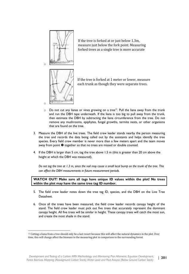
| 201Development and Testing of a Carbon MRV Methodology and Monitoring Plan: Allometric Equation Development, Forest Biomass Mapping (Aboveground Carbon Stock), Water Level and Peat Anaysis (Below Ground Carbon Stock)
o
o
o Do not cut any lianas or vines growing on a tree12. Pull the liana away from the trunk and run the DBH tape underneath. If the liana is too big to pull away from the trunk, then estimate the DBH by subtracting the liana circumference from the tree. Do not remove any mushrooms, epiphytes, fungal growths, termite nests, or other organisms that are found on the tree.
3. Measure the DBH of the live trees. The field crew leader stands nearby the person measuring the tree and records the data being called out by the assistants and helps identify the tree species. Every field crew member is never more than a few meters apart and the team moves away from point together so that no trees are missed or double counted.
4. If the DBH is larger than 5 cm, tag the tree above 1.5 m (this is greater than 20 cm above the height at which the DBH was measured). Do not tag the tree at 1.3 m, since the nail may cause a small local bump on the trunk of the tree. This can affect the DBH measurements in future measurement periods.
WATCH OUT! Make sure all tags have unique ID values within the plot! No trees within the plot may have the same tree tag ID number.
5. The field crew leader notes down the tree tag ID, species, and the DBH on the Live Tree
Datasheet.
6. Once all the trees have been measured, the field crew leader records canopy height of the stand. The field crew leader must pick out five trees that accurately represent the dominant canopy height. All five trees will be similar in height. These canopy trees will catch the most sun, and create the most shade in the stand.
12 Cutting a liana from a tree should only be a last resort because this will affect the natural dynamics in the plot. Over time, this will change affect the biomass in the measuring plot in comparison to the surrounding forest.
If the tree is forked at or just below 1.3m, measure just below the fork point. Measuring forked trees as a single tree is more accurate
f f b
If the tree is forked at 1 meter or lower, measure each trunk as though they were separate trees.
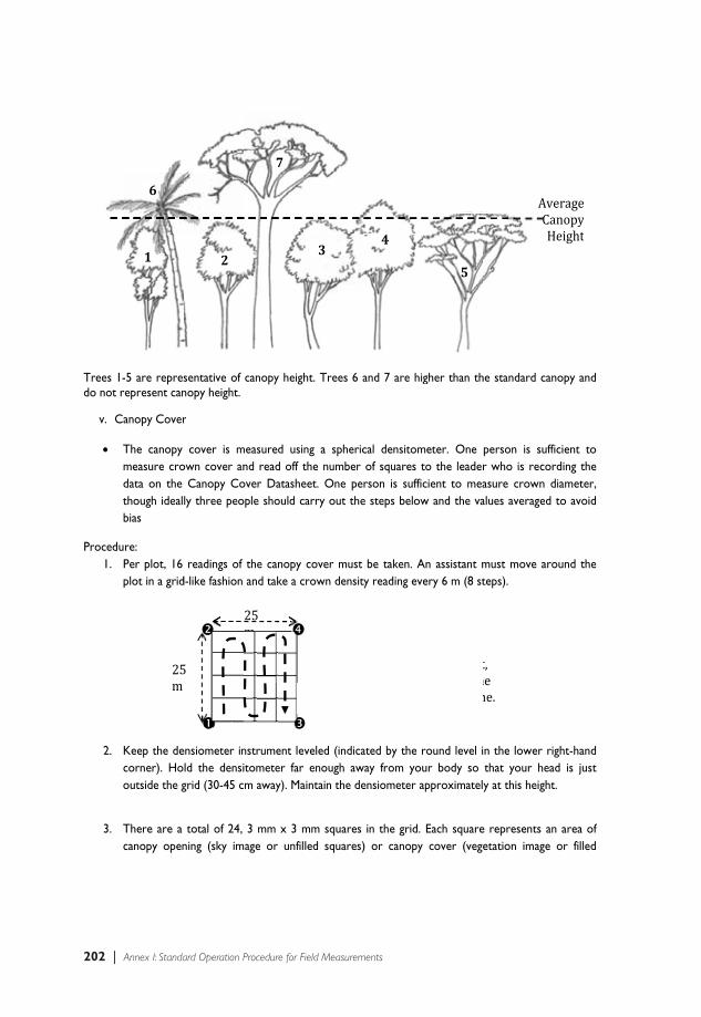
202 | Annex I: Standard Operation Procedure for Field Measurements
Trees 1-do not r
v. Ca
• Tmdtb
Procedu1. P
p
2. Kco
3. T
c
-5 are represrepresent can
anopy Cover
The canopy measure crodata on the though ideallbias
re: Per plot, 16 plot in a grid
Keep the decorner). Hooutside the g
There are a canopy open
6
1
25m
sentative of nopy height.
r
cover is mown cover an
Canopy Coly three peo
readings of d-like fashion
ensiometer inld the densigrid (30-45 c
total of 24, ning (sky im
2
5
canopy heigh
measured usind read off tover Datasheople should c
the canopy and take a c
nstrument leitometer far m away). Ma
3 mm x 3 mage or unfil
7
25 m
ht. Trees 6 a
ng a sphericthe number eet. One pecarry out the
cover must crown density
veled (indicaenough aw
aintain the de
mm squares led squares)
3
To get 16the assistplot simi
and 7 are hig
cal densitomof squares trson is suffice steps below
be taken. Aty reading eve
ated by the rway from youensiometer a
in the grid. ) or canopy
4
6 readings ftant walks ilarly to the
gher than th
meter. One to the leadercient to meaw and the va
An assistant mery 6 m (8 st
round level iur body so approximately
Each squarecover (vege
5
for the plotthrough the dashed lin
he standard c
person is sur who is recasure crownalues average
must move ateps).
n the lower that your hy at this heig
e represents etation imag
AC
t, he ne.
canopy and
ufficient to cording the n diameter, ed to avoid
around the
right-hand ead is just
ght.
an area of ge or filled
Average Canopy Height
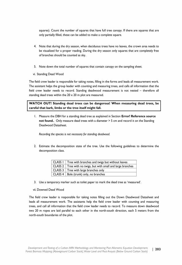
| 203Development and Testing of a Carbon MRV Methodology and Monitoring Plan: Allometric Equation Development, Forest Biomass Mapping (Aboveground Carbon Stock), Water Level and Peat Anaysis (Below Ground Carbon Stock)
squares). Count the number of squares that have full tree canopy. If there are squares that are only partially filled, these can be added to make a complete square.
4. Note that during the dry season, when deciduous trees have no leaves, the crown area needs to
be visualized for a proper reading. During the dry season only squares that are completely free of branches should be counted as sky.
5. Note down the total number of squares that contain canopy on the sampling sheet.
vi. Standing Dead Wood
The field crew leader is responsible for taking notes, filling in the forms and leads all measurement work. The assistant helps the group leader with counting and measuring trees, and calls all information that the field crew leader needs to record. Standing deadwood measurement is not nested – therefore all standing dead trees within the 20 x 20 m plot are measured.
WATCH OUT! Standing dead trees can be dangerous! When measuring dead trees, be careful that bark, limbs or the tree itself might fall.
1. Measure the DBH for a standing dead tree as explained in Section Error! Reference source not found.. Only measure dead trees with a diameter > 5 cm and record it on the Standing Deadwood Datasheet. Recording the species is not necessary for standing deadwood.
2. Estimate the decomposition state of the tree. Use the following guidelines to determine the decomposition class.
CLASS 1 Tree with branches and twigs but without leavesCLASS 2 Tree with no twigs, but with small and large branches CLASS 3 Tree with large branches only CLASS 4 Bole (trunk) only, no branches
3. Use a temporary marker such as toilet paper to mark the dead tree as ‘measured’.
vii. Downed Dead Wood
The field crew leader is responsible for taking notes filling out the Down Deadwood Datasheet and leads all measurement work. The assistants help the field crew leader with counting and measuring trees, and call all information that the field crew leader needs to record. To measure down deadwood two 20 m ropes are laid parallel to each other in the north-south direction, each 5 meters from the north-south boundaries of the plot.

204 | Annex I: Standard Operation Procedure for Field Measurements
Figure 12plot
1. Tmd
2. We
iD
3. I
4. A
5. Im
13 The hol
2. The image
The field crem east of podirectly nort
Walk along equal to 10 c10 cm in diaintersecting Deadwood D
a. the ob. estimc. the ld. the de. the r
If the log is h
Assign each p
CLASS 1 SCLASS 2 ICLASS 3 R
If a piece omeasuremen
llow portion in
of necromas
ew leader waoint . The th from the p
the rope ancm diameter ameter at thdown dead
Datasheet:
outer circummated circumength of the density class,rope number
hollow, estim
piece of dead
Sound woodIntermediateRotten/crumof down dents for rope
n the volume es
s plot and the
alks betweenlocation for
points indicat
d analyze eaat the point
he point whedwood the
mference at thmference of h
log, , and r that interse
mate the circu
d wood to o
; a machete e wood; a ma
mbly wood; a eadwood is 1.
stimates will be
e determinat
point andr rope 2 is 5ted by the fie
ach intersectthe log cros
ere it crossefield crew
he middle of hollow at the
ects the log.
umference of
ne of three d
does not sinachete sinks pmachete cutto long th
e excluded in th
ion of each n
d point an5 m west ofeld crew lead
ting piece ofsses the ropees the line, isleader reco
the log, e middle of th
f the hollow
density classe
nk into the wpartly into thts through thhat it touch
he calculations
ecromass bas
nd marks thef point . Tder.
f down deade. Down deas not measu
ords the fol
he log,
at the middl
es.
wood in a singhe piece in a he piece in a hes both ro
s
sed on its loca
e location foThe ropes ar
dwood greatdwood that red. For eaclowing on t
e length of th
gle strike single strike single strike
opes, only r
ation in the
r rope 1, 5 e then laid
ter than or is less than ch piece of the Down
he wood13
record the
| 205Development and Testing of a Carbon MRV Methodology and Monitoring Plan: Allometric Equation Development, Forest Biomass Mapping (Aboveground Carbon Stock), Water Level and Peat Anaysis (Below Ground Carbon Stock)
6. Use a temporary marker such as toilet paper to mark the intersecting piece of wood as ‘measured’.
viii. Logged Tree Stumps
The field crew leader is responsible for taking notes, filling out forms and leading all measurement work. The assistants help the field crew leader by counting and measuring trees, and calling out all information that the field crew leader needs to record. All logged tree stumps greater than 15.7 cm in circumference at the top are measured within the 20 x 20 m plot.
1. Note down the height and the diameter at the top of each logged tree stump on the Logged Tree Stump Datasheet.
2. Assign and note down the density of the tree stump on the “logged tree stump data sheet”. Use a machete to determine the decomposition class, using the following guidelines.
CLASS 1 Sound wood; a machete cannot sink into the wood in a single strike CLASS 2 Intermediate wood; a machete sinks partly into the piece in a single strike CLASS 3 Rotten/crumbly wood; a machete cuts through the piece in a single strike
3. Use toilet paper to mark the dead tree as “measured”.
ix. Aboveground Non-tree Living and Standing Dead Biomass
1. In the undisturbed site of each subsample plot the field crew leader carefully measures a circle around the subsample point location identified in Section iii with a radius of 0.5 m. The assistants help the field crew leader by laying a rope on the ground around the circumference of the circle measured by the field crew leader.
2. The field crew leader weighs the empty gunnysack, and records the weight of the empty
gunnysack on the Aboveground Non-tree Biomass and Seedling Datasheet.
3. The community workers collect all aboveground non-tree plants including, herbs, grasses,
rattan, ferns, etc that are found within the circle. This is done by clipping all the plants down to ground level and placing them in the gunnysack. Woody non-tree plants such as shrubs and bushes are considered non-tree if they do not have the potential to reach a height of 2 meters and a DBH of 5 cm. Collecting is done by clipping all the plants down to mineral soil and placing them in the gunnysack. Ferns, dry grasses, and dead herbs are collected, while leaves, twigs and lying dead herbs that have fallen are not. All seedlings, saplings and trees are left in the circle. Only plants that are within the circle or the two meter space above it are collected. If a plant is hanging into the circle, but the roots are growing outside the circle, only the part of the plant hanging into the circle is collected. Likewise, if a plant is growing inside the circle, but hanging out of the circle, only the part inside the circle is collected.
4. The gunnysack, full of living and once living non-tree biomass, is weighed with the spring scale
and recorded by the team leader on the designated location on the datasheet.

206 | Annex I: Standard Operation Procedure for Field Measurements
WATCtrees, s
5. Ttlftalt
WAfieldleadas it
6. Tr
CH OUT: Waplings or s
The communtree biomassleader then sfound in the than 100 g oabovegroundlabeled with to the lab to
ATCH OUTd laboratorder must cat comes bac
The gunnysaremove any
When removseedlings w
nity workerss into pieces selects a 100gunnysack. I
of non-tree d non tree bthe plot ID determine m
T: The samry and weigarefully track from the
ack is emptieexcess water
ving all abowithin the su
s use the clipno bigger th
0 g sample ofIf the materibiomass, tak
biomass in thand sample
moisture con
mple of aboghed more ansport the e field.
ed of its contr.
oveground ubsample.
ppers to cuthan 5 cm by f material thaal is very weke it all. If the subsamplplot number
ntent and dry
out 100g maccuratelysample, an
tents away fr
Subsampletemporary
Subsampboundar0.5 m ra
non-tree b
t all the colle5 cm and mat is represeet, try to shathere is none point. Thisr (1, 2 or 3) y mass).
must be cary with the cnd reweigh
rom the sub
e point y marker
ple ry of adius
iomass, be
ected living aix it up in thntative of th
ake off excese, check thes sample is by the team
efully transcompact sc
h on the co
bsample point
careful not
and standing e gunnysacke material co
ss water. If the box that tput in a clot
m leader (to b
sported bacale. The Fmpact scal
t, and is sha
t to harm
dead non-. The team omposition here is less there is no th bag and be brought
ack to the Field crew e as soon
ken out to
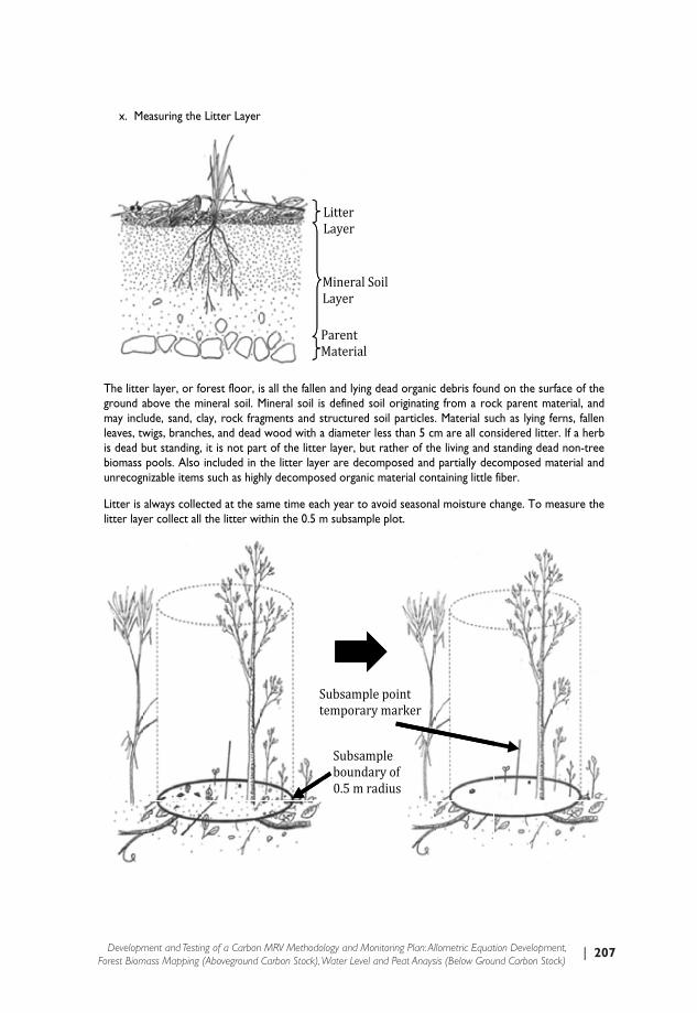
| 207Development and Testing of a Carbon MRV Methodology and Monitoring Plan: Allometric Equation Development, Forest Biomass Mapping (Aboveground Carbon Stock), Water Level and Peat Anaysis (Below Ground Carbon Stock)
x. M
The litteground amay inclleaves, twis dead bbiomass unrecogn
Litter is litter laye
easuring the
er layer, or foabove the mude, sand, cwigs, branchbut standing,pools. Also
nizable items
always collecer collect all
Litter Layer
orest floor, imineral soil. M
lay, rock frages, and dead it is not parincluded in t
s such as high
cted at the sthe litter wi
r
s all the falleMineral soil igments and wood with rt of the littethe litter layhly decompo
ame time eaithin the 0.5
en and lying dis defined sostructured sa diameter l
er layer, but yer are decomosed organic
ach year to avm subsample
Litter Layer
Mineral SoLayer
Parent Material
Subsampletemporary
Subsampboundar0.5 m ra
dead organicoil originatingsoil particles.ess than 5 cmrather of thmposed and material con
void seasonae plot.
oil
e point y marker
ple ry of adius
c debris foung from a roc. Material sum are all cone living and spartially dec
ntaining little
al moisture c
d on the surck parent mach as lying f
nsidered littestanding deacomposed mfiber.
change. To m
rface of the aterial, and ferns, fallen er. If a herb ad non-tree material and
measure the

208 | Annex I: Standard Operation Procedure for Field Measurements
1. Wiw
2. Tpb
3. W
4. Tbsti(m
xi. Co
All seedsubsamp
1. TTm
2. Tw
Sbr
Weigh the eis important water may ha
The assistantpruning sheabiomass, only
Weigh the gu
The commubigger than 5sample of mathere is less in the subplo(1, 2 or 3) bymass).
ounting Seed
lings (trees wple point.
The field creThe assistantm radius aro
The assistantwhen
Subsampltemporary
Subsampleboundary oradius
mpty gunnysto reweigh
ave saturated
ts collect allars are usedy the litter w
unnysack full
nity workers5 cm by 5 cmaterial that ithan 100 g o
ot. This sampy the team le
dlings
with a DBH
ew leader carts help the t
ound the subs
ts count the
le point y marker
of 1 m
sack and recothe gunnysad the gunnys
l the litter w to cut the
within the cir
of litter and
s use the prm and mix its representaof litter, takeple is put in eader (to be
less than o
refully measuteam leader bsample point
e number of
ord the emptck, though it
sack, giving it
within the cilitter stickin
cle is measur
d record the
runing sheart up in the guative of the me it all. If thera bag and lab
e brought to
r equal to 1
ures a circle by moving tht.
seedlings fro
ty weight ont was just wt a much heav
rcle and plang out of thred.
weight on th
s to cut all unnysack. Thmaterial comre is none, cbeled with ththe lab to de
cm) are co
with a 1 m he rope outw
om outside t
•
•
•
the Litter Leighted in sevier weight.
ace it in the he circle. Sim
he datasheet.
the collectehe team leadmposition fou
heck the boxhe plot ID anetermine mo
ounted within
radius arounward to form
the circle an
In the figurdashed linesubsamplespace abovThe tallest over 2 metDBH greateIn this subsare 5 seedlcrew leadesmall seedlof seedling
ayer datasheection ix abo
gunnysack. milar to non-
.
ed litter intoer then selec
und in the gux that there nd sample ploisture conte
n a 1 m radi
nd the subsamm a new circ
d only enter
re to the lefe represente area and ave it. seedling, thters does noer than 1 cmsample poilings. The fier helps to ilings. The ngs is record
eet. Note it ove. Excess
A knife or -tree living
pieces no cts a 100 g unnysack. If is no litter ot number
ent and dry
ius of each
mple point. le with a 1
r the circle necessary.
ft the ts the a 2 m
hough ot have a m. nt there ield identify number ed on

| 209Development and Testing of a Carbon MRV Methodology and Monitoring Plan: Allometric Equation Development, Forest Biomass Mapping (Aboveground Carbon Stock), Water Level and Peat Anaysis (Below Ground Carbon Stock)
1. All data is recorded by the team leader on the designated location on the Aboveground Non-tree Biomass and Seedling Datasheet.

210 | Annex I: Standard Operation Procedure for Field Measurements
Perm
Origina
Measur
Name
Sheet c
File ID
File ID
File ID
File ID
File ID
Was thIf yes, w
Project
Katingan
manent P
al GPS coo
rement tim
of field cr
checked b
of photo
of photo
of photo
of photo
of photo
he originalwhy? ___
___
ID Poi
n
3 replicate1. x: _____2x: ______3.x: _____
N
Peat Wa
ordinate o
me and da
rew leader
by:_______
facing No
facing Eas
facing Sou
facing We
showing G
l position __________________
int ID
es of GPS co___________________________________
atertabl
of point
ate: ____
r: ____
_________
orth from
st from
uth from
est from
GPS coord
of point __________________
GP
WatertDistancpipe):
Distancground:
Depth o
oordinates ________y: _______ y:_________y:__
e Monit
:x:______
_________
_________
______ D
: ____
: ____
: ____
: ____
dinates: __
changed__________________
PS serial num
table depce b (top
ce a (to
of watertab
of point____________________________________
toring P
_________
_________
_________
Data entere
_________
_________
_________
_________
_________
d? Yes __________________
mber
pth (metep of wate
p of pip
ble (b-a)
in WGS84U_______________________________
Point (1 s
___y:____
_________
_________
ed by: ___
_________
_________
_________
_________
________
, No ________________
ers)er to top
e to top
UTM 49S:_
sheet / p
_________
________
________
_________
_________
_________
_________
_________
_________
__________________
p of
p of
package
_______
_____
_____
_____
____
____
____
____
_____
____________
e)
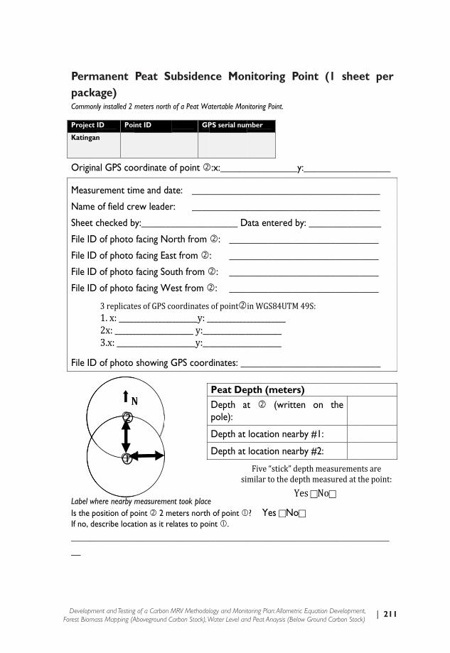
| 211Development and Testing of a Carbon MRV Methodology and Monitoring Plan: Allometric Equation Development, Forest Biomass Mapping (Aboveground Carbon Stock), Water Level and Peat Anaysis (Below Ground Carbon Stock)
PermpackaCommon
Project
Katingan
Origina
Measur
Name
Sheet c
File ID
File ID
File ID
File ID
File ID
Label whIs the poIf no, de
________
manent age) ly installed 2
ID Poi
n
al GPS coo
rement tim
of field cr
checked b
of photo
of photo
of photo
of photo
of photo
here nearby mosition of pescribe locat
_________
3 replicate1. x: _____2x: ______3.x: _____
N
Peat Su
meters north
int ID
ordinate o
me and da
rew leader
by:_______
facing No
facing Eas
facing Sou
facing We
showing G
measuremenoint 2 mtion as it re
________
es of GPS co___________________________________
N
ubsiden
of a Peat Wa
GP
of point
ate: ____
r: ____
_________
orth from
st from
uth from
est from
GPS coord
nt took placeeters north
elates to poi
_________
oordinates ________y: _______ y:_________y:__
nce Mon
atertable Mon
PS serial num
:x:______
_________
_________
______ D
: ____
: ____
: ____
: ____
dinates: __
e h of point int .
_________
Peat DeDepth atpole):
Depth at
Depth at
of point____________________________________
si
nitoring
nitoring Point.
mber
_________
_________
_________
Data entere
_________
_________
_________
_________
_________
? Yes
_________
pth (mett (wr
location n
location n
in WGS84U_______________________________
Five “stickmilar to the
g Point
___y:____
_________
_________
ed by: ___
_________
_________
_________
_________
________
No
_________
ters)ritten on
nearby #1:
nearby #2:
UTM 49S:_
k” depth me depth meYes N
(1 shee
_________
________
________
_________
_________
_________
_________
_________
_________
________
n the
: : easuremeneasured at tNo
et per
_______
_____
_____
_____
____
____
____
____
_____
_______
nts are the point:

212 | Annex I: Standard Operation Procedure for Field Measurements
Units in cmAugur bottom Direction of augur handle
Sketch, Description and Sample Collection (1 sheet for per plot)
Project ID Point ID GPS serial number
Katingan
Munsell Color Chart Color Peat Color Soil Color
Hue:
Value:
Chroma:
N
<2m
2m
Was a sample taken at this location? Yes NoIf yes, please record: Strata Name: ___________________________________ Coordinates in WGS84 UMT49S: X:_____________________, Y: _____________________ Field Crew Leader: _______________________________ Time and Date: __________________________________
Core ID Color Depth (m) Maturity
PeatMaturity (circle one): Fibric, Hemic or Sapric

| 213Development and Testing of a Carbon MRV Methodology and Monitoring Plan: Allometric Equation Development, Forest Biomass Mapping (Aboveground Carbon Stock), Water Level and Peat Anaysis (Below Ground Carbon Stock)
Description of vegetation of the plot and soil type:
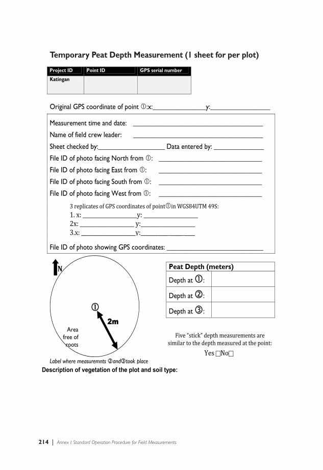
214 | Annex I: Standard Operation Procedure for Field Measurements
Temporary Peat Depth Measurement (1 sheet for per plot)
Project ID Point ID GPS serial number
Katingan
Original GPS coordinate of point :x:________________y:__________________
Measurement time and date: _______________________________________
Name of field crew leader: _______________________________________
Sheet checked by:____________________ Data entered by: _______________
File ID of photo facing North from : _______________________________
File ID of photo facing East from : _______________________________
File ID of photo facing South from : _______________________________
File ID of photo facing West from : _______________________________
File ID of photo showing GPS coordinates: _____________________________
Label where measuremnts and took place
Peat Depth (meters)
Depth at :
Depth at :
Depth at :
Area free of roots
2m
N
3 replicates of GPS coordinates of point in WGS84UTM 49S:1. x: ______________________y: ______________________ 2x: ______________________ y:______________________ 3.x: ______________________y:______________________
Five “stick” depth measurements are similar to the depth measured at the point:
Yes No
Description of vegetation of the plot and soil type:

| 215Development and Testing of a Carbon MRV Methodology and Monitoring Plan: Allometric Equation Development, Forest Biomass Mapping (Aboveground Carbon Stock), Water Level and Peat Anaysis (Below Ground Carbon Stock)
Biomass Inventory Data Coversheet (1 sheet per plot)
Project ID Plot ID GPS serial number
Katingan
Measurement time and date: _____________________ Name of field crew leader: _____________________ File ID of picture from North: _____________________ File ID of picture from East: _____________________ File ID of picture from South: _____________________ File ID of picture from West: _____________________ File ID of picture from Up: _____________________ Slope and aspect from point : _____________________ Was the original position of point changed? Yes No If yes, why? ________________________________________________________
_______________________ _______________________ _____________ ________________ _______________________ _______________________ _____________ ________________ _______________________ _______________________ _____________ ________________ _______________________ _______________________ _____________ ________________ _______________________ _______________________ _____________ ________________ _______________________ _______________________ _____________ ________________ _______________________ _______________________ _____________ ________________ _______________________ _______________________ _____________ ________________ _______________________ _______________________ _____________ ________________ _______________________ _______________________ _____________ ________________ _______________________ _______________________ _____________ ________________ _______________________ _______________________ _____________ ________________
GPSUTMcoordinates(in WGS84, with UTM 48 N)3 readings of each corner GPS coordinates:
WaypointID
PictureIDTaken of screen
Original GPS coordinate of :
Data Review (To be filled out when plot
is complete)
Sheet checked by: __________________ Data entered by: __________________

216 | Annex I: Standard Operation Procedure for Field Measurements
Sketch of Plot (1 sheet per plot)
Project ID Plot ID GPS serial number
Katingan
Name of drawer: _____________________________
Include significant features, both inside and outside of the plot.
N
Description of forest status of the plot:
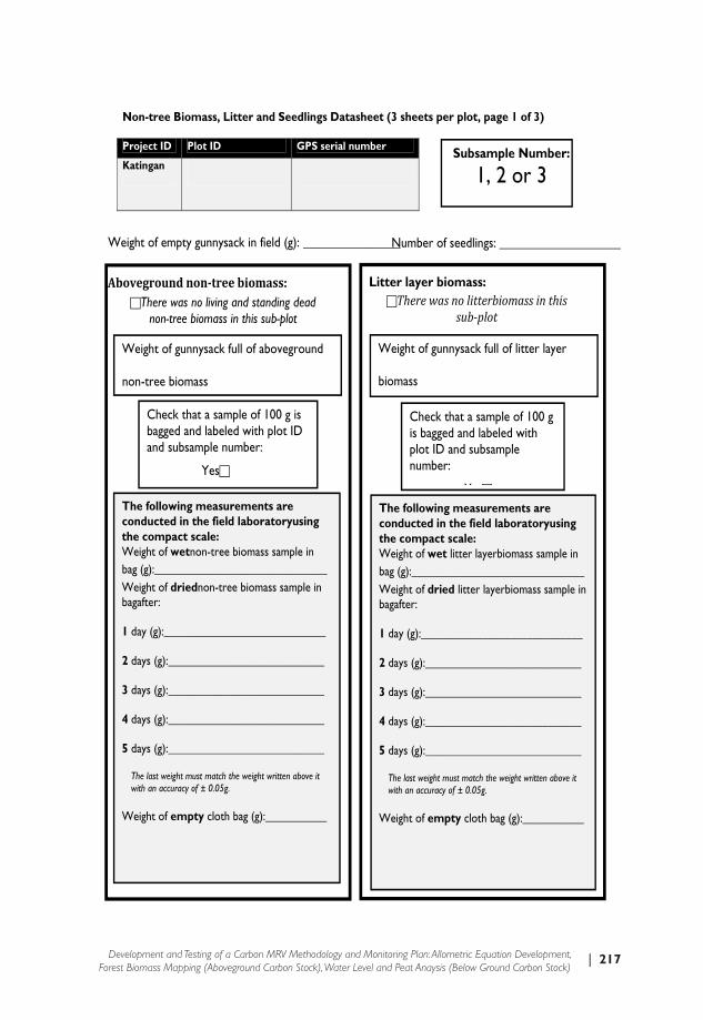
| 217Development and Testing of a Carbon MRV Methodology and Monitoring Plan: Allometric Equation Development, Forest Biomass Mapping (Aboveground Carbon Stock), Water Level and Peat Anaysis (Below Ground Carbon Stock)
Non-tree Biomass, Litter and Seedlings Datasheet (3 sheets per plot, page 1 of 3)
Project ID Plot ID GPS serial number
Katingan
Litter layer biomass:
Abovegroundnon‐treebiomass:
Subsample Number:
1, 2 or 3
Check that a sample of 100 g is bagged and labeled with plot ID and subsample number:
Yes
Weight of gunnysack full of aboveground
non-tree biomass
The following measurements are conducted in the field laboratoryusing the compact scale: Weight of wetnon-tree biomass sample in
bag (g):_______________________________
Weight of driednon-tree biomass sample in bagafter:
1 day (g):_____________________________
2 days (g):____________________________
3 days (g):____________________________
4 days (g):____________________________
5 days (g):____________________________
The last weight must match the weight written above it with an accuracy of ± 0.05g.
Weight of empty cloth bag (g):___________
There was no living and standing dead non-tree biomass in this sub-plot
Therewasnolitterbiomassinthissub‐plot
Weight of empty gunnysack in field (g): ________________
Weight of gunnysack full of litter layer
biomass
Check that a sample of 100 g is bagged and labeled with plot ID and subsample number:
YThe following measurements are conducted in the field laboratoryusing the compact scale: Weight of wet litter layerbiomass sample in
bag (g):_______________________________
Weight of dried litter layerbiomass sample in bagafter:
1 day (g):_____________________________
2 days (g):____________________________
3 days (g):____________________________
4 days (g):____________________________
5 days (g):____________________________
The last weight must match the weight written above it with an accuracy of ± 0.05g.
Weight of empty cloth bag (g):___________
Number of seedlings: ____________________
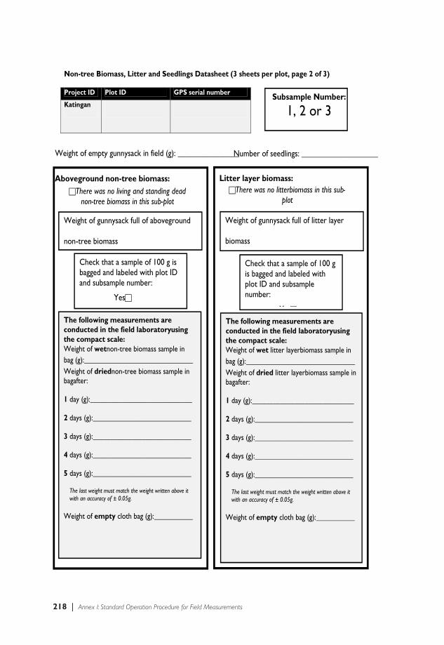
218 | Annex I: Standard Operation Procedure for Field Measurements
Non-tree Biomass, Litter and Seedlings Datasheet (3 sheets per plot, page 2 of 3)
Project ID Plot ID GPS serial number
Katingan
Litter layer biomass:
Aboveground non-tree biomass:
Subsample Number:
1, 2 or 3
Check that a sample of 100 g is bagged and labeled with plot ID and subsample number:
Yes
Weight of gunnysack full of aboveground
non-tree biomass
The following measurements are conducted in the field laboratoryusing the compact scale: Weight of wetnon-tree biomass sample in
bag (g):_______________________________
Weight of driednon-tree biomass sample in bagafter:
1 day (g):_____________________________
2 days (g):____________________________
3 days (g):____________________________
4 days (g):____________________________
5 days (g):____________________________
The last weight must match the weight written above it with an accuracy of ± 0.05g.
Weight of empty cloth bag (g):___________
There was no living and standing dead non-tree biomass in this sub-plot
There was no litterbiomass in this sub-plot
Weight of empty gunnysack in field (g): ________________
Weight of gunnysack full of litter layer
biomass
Check that a sample of 100 g is bagged and labeled with plot ID and subsample number:
YThe following measurements are conducted in the field laboratoryusing the compact scale: Weight of wet litter layerbiomass sample in
bag (g):_______________________________
Weight of dried litter layerbiomass sample in bagafter:
1 day (g):_____________________________
2 days (g):____________________________
3 days (g):____________________________
4 days (g):____________________________
5 days (g):____________________________
The last weight must match the weight written above it with an accuracy of ± 0.05g.
Weight of empty cloth bag (g):___________
Number of seedlings: ____________________

| 219Development and Testing of a Carbon MRV Methodology and Monitoring Plan: Allometric Equation Development, Forest Biomass Mapping (Aboveground Carbon Stock), Water Level and Peat Anaysis (Below Ground Carbon Stock)
Non-tree Biomass, Litter and Seedlings Datasheet (3 sheets per plot, page 3 of 3)
Project ID Plot ID GPS serial number
Katingan
Litter layer biomass:
Aboveground non-tree biomass:
Subsample Number:
1, 2 or 3
Check that a sample of 100 g is bagged and labeled with plot ID and subsample number:
Yes
Weight of gunnysack full of aboveground
non-tree biomass
The following measurements are conducted in the field laboratoryusing the compact scale: Weight of wetnon-tree biomass sample in
bag (g):_______________________________
Weight of driednon-tree biomass sample in bagafter:
1 day (g):_____________________________
2 days (g):____________________________
3 days (g):____________________________
4 days (g):____________________________
5 days (g):____________________________
The last weight must match the weight written above it with an accuracy of ± 0.05g.
Weight of empty cloth bag (g):___________
There was no living and standing dead non-tree biomass in this sub-plot
There was no litterbiomass in this sub-plot
Weight of empty gunnysack in field (g): ________________
Weight of gunnysack full of litter layer
biomass
Check that a sample of 100 g is bagged and labeled with plot ID and subsample number:
YThe following measurements are conducted in the field laboratoryusing the compact scale: Weight of wet litter layerbiomass sample in
bag (g):_______________________________
Weight of dried litter layerbiomass sample in bagafter:
1 day (g):_____________________________
2 days (g):____________________________
3 days (g):____________________________
4 days (g):____________________________
5 days (g):____________________________
The last weight must match the weight written above it with an accuracy of ± 0.05g.
Weight of empty cloth bag (g):___________
Number of seedlings: ____________________

220 | Annex I: Standard Operation Procedure for Field Measurements
Live Tree Datasheet for the 20 x 20 m Plot (2 sheets per plot, page 1 of 2)
Project ID Plot ID GPS serial number
Katingan
Trees that represent the canopy (5 trees per plot) Height (m) DBH (cm)
1
2
3
4
5
Number Tree Tag ID Species DBH (cm) 1
2
3
4
5
6
7
8
9
10
11
12
13
14
15
16
17
18
TherearenotreeswithaDBHgreaterthanorequalto15cminthisplot

| 221Development and Testing of a Carbon MRV Methodology and Monitoring Plan: Allometric Equation Development, Forest Biomass Mapping (Aboveground Carbon Stock), Water Level and Peat Anaysis (Below Ground Carbon Stock)
Live Tree Datasheet for the 20 x 20 m Plot (2 sheets per plot, page 2 of 2)
Project ID Plot ID GPS serial number
Katingan
Number Tree Tag ID Species DBH (cm) 19
20
21
22
23
24
25
26
27
28
29
30
31
32
33
34
35
36
37
38
39
40
41
42
43

222 | Annex I: Standard Operation Procedure for Field Measurements
Live Tree Datasheet for 10 x 10 m Nested Plot (2 sheets per plot, p. 1/2)
Project ID Plot ID GPS serial number
Katingan
Number Tree Tag ID Species DBH (cm)1
2
3
4
5
6
7
8
9
10
11
12
13
14
15
16
17
18
19
20
21
22
23
24
25
TherearenotreeswithaDBHfrom5to15cminthisplot

| 223Development and Testing of a Carbon MRV Methodology and Monitoring Plan: Allometric Equation Development, Forest Biomass Mapping (Aboveground Carbon Stock), Water Level and Peat Anaysis (Below Ground Carbon Stock)
Error! Reference source not found.Live Tree Datasheet for 10 x 10 m Nested Plot (2 sheets per plot, p.2/2)
Project ID Plot ID GPS serial number
Katingan
Number Tree Tag ID Species CBH (cm) 27
38
29
30
31
32
33
34
35
36
37
38
39
40
41
42
43
44
45
46
47
48
49
50
51

224 | Annex I: Standard Operation Procedure for Field Measurements
Standing Deadwood Datasheet (1 sheetper plot)
Project ID Plot ID GPS serial number
Katingan
CLASS 1
Tree with branches and twigs but without leaves
CLASS 2
Tree with no twigs, but with small and large branches
CLASS 3
Tree with large branches only
CLASS 4
Bole (trunk) only, no branches
DBH (cm)
Decomposition class(1, 2, 3, or 4) Height
TherearenostandingdeadtreeswithaDBHgreaterthanorequalto5cminthisplot

| 225Development and Testing of a Carbon MRV Methodology and Monitoring Plan: Allometric Equation Development, Forest Biomass Mapping (Aboveground Carbon Stock), Water Level and Peat Anaysis (Below Ground Carbon Stock)
Downed Deadwood Datasheet (1 sheetper plot)
Project ID Plot ID GPS serial number
Katingan
CLASS 1Sound wood; a machete does not sink into the wood in a single strike
CLASS 2Intermediate wood; a machete sinks partly into the piece in a single strike
CLASS 3Rotten/crumbly wood; a machete cuts through the piece in a single strike
Line (1 or 2)
Length (m)
Outer circumference measured at log center (cm)
Estimated circumference of hollow at log center (cm)
Density class (1, 2, or 3)
Therearenodowndeadtreeswithacircumferencegreaterthanorequalto31.4cmatthetransectrope

226 | Annex I: Standard Operation Procedure for Field Measurements
Canopy Cover Datasheet (1 sheetper plot)
Project ID Plot ID GPS serial number
Katingan
Operator 1 Operator 2 Operator 3
Grid Cell
# of sky squares
# of canopy squares
# of sky squares
# of canopy squares
# of sky squares
# of canopy squares
1 2 3 4 5 6 7 8 9 10 11 12 13 14 15 16
25 m
25 m
16 15 14 13 12
11 10 9 8
7 6 5 4
3 2 1

| 227Development and Testing of a Carbon MRV Methodology and Monitoring Plan: Allometric Equation Development, Forest Biomass Mapping (Aboveground Carbon Stock), Water Level and Peat Anaysis (Below Ground Carbon Stock)
Logged Tree Stump Datasheet (1 sheetper plot)
Project ID Plot ID GPS serial number
CCI - Katingan
CLASS 1
Sound wood; a machete does not sink into the wood in a single strike
CLASS 2
Intermediate wood; a machete sinks partly into the piece in a single strike
CLASS 3
Rotten/crumbly wood; a machete cuts through the piece in a single strike
Circumference at top of stump (cm)
Decomposition class(1, 2, 3, or 4) Height
TherearenologgedtreestumpswithaDBHgreaterthanorequalto5cminthisplot

228 | Annex I: Standard Operation Procedure for Field Measurements

| 229Development and Testing of a Carbon MRV Methodology and Monitoring Plan: Allometric Equation Development, Forest Biomass Mapping (Aboveground Carbon Stock), Water Level and Peat Anaysis (Below Ground Carbon Stock)
Annex 2: Standard Operation Procedure for
AllometricDevelopment and Verification
Procedure to develop and verify allometric equations for an avoided peatland
conversion project in Central Kalimantan Province, Indonesia
Version 3-0
230 | Annex 2: Standard OperationProcedure for Allometric Development and Verification
Acronyms and Definitions cm centimeter DBH Diameter at Breast Height (the diameter measurement of the tree at 1.3 m above the
ground) Forest An area with a tree crown cover of at least 10 %, of at least 1 ha in size, and a minimum
tree height of 5 meters. GPG Good Practice Guidance for Land-Use Land-Use Change and Forestry GPS Global Positioning System (often referred to a handheld device that supports GPS) IPCC Intergovernmental Panel on Climate Change m Meter Peat An accumulation of partially decayed vegetation matter of at least 0.3 meters thick at
ground surface or below water level. PVC Polyvinyl chloride, (a type of plastic easily used for permanent watertable measuring
point and subsidence point installation. kg Kilogram UTM Universal Transverse Mercator (Set to UTM49S for Katingan District, Central
Kalimantan Province, Indonesia)
| 231Development and Testing of a Carbon MRV Methodology and Monitoring Plan: Allometric Equation Development, Forest Biomass Mapping (Aboveground Carbon Stock), Water Level and Peat Anaysis (Below Ground Carbon Stock)
1. Background In addition to executing the biomass inventories, the allometric equation14 selected for estimating biomass from measured tree DBH and/or heights must be explicitly verified using empirical data. This has to occur only once. However, the verification of an allometric equation remains a crucial part of the field measurements. The allometric equation must be tested as small errors can multiply significantly as the scale of estimation increases. If a specific allometric equation does not predict biomass conservatively, a different equation must be selected. When no existing allometric equation is appropriate, a new allometric equation must be developed. Developing a new allometric equation is lengthy and time consuming process. Procedures to select a valid allometric equation and test the allometric equation with field data are described in this document. Use the following hierarchy to select the most appropriate allometric equation:
1. Allometric equations developed by project proponents. 2. Allometric equations developed locally by groups other than project proponents. 3. Allometric equations developed for forest types that are similar to the ones in the project as
found in found in Appendix C of Pearson et al. (2005), or Tables 4.A.1. and 4.A.2. of the GPG LULUCF.
After the allometric equation is selected it must be verified in the field.
2. Equation Selection The following conditions must be met for an appropriate allometric equation(s).
1. The proposed equation(s) was/were developed from trees where the largest and smallest DBH of the trees fall within the DBH range of 95% of the trees within the project areas.
2. The proposed equation(s) must have an r2 value of greater than 0.5 (50%) and a p-value that is significant at 95% confidence level as reported in the source publications.
3. If the proposed equation(s) was/were derived from data solely from within the reference region then such equations can be used. If the proposed equation(s) was/were derived outside of the reference region, project proponents must justify the similarity in climatic, edaphic, geographical and species composition between the project area and the location from where the equations were derived. The source publication must include an estimate of the uncertainty or sufficient data to estimate the uncertainty. If this uncertainty is within ±15% of the mean values and is not biased in a non-conservative manner (i.e., the equation(s) do(es) not systematically overestimate the project net anthropogenic removals by sinks), the equation(s) may be used.
4. If no reliable equation exists, select most appropriate equation from Chave et al. (2005) or Ketterings et al. (2001).
5. The selected allometric equation must be verified with field measurements according to the procedures in this SOP.
3. Field Measurement The allometric equation can be verified using either destructive sampling or using limited measurements. Field measurement is required for both of these methods. However, only one of the two approaches must be followed. It is preferred to use Destructive Sampling. However, in case where destructive sampling is not feasible or practical, Limited Measurements is allowed, but is not very precise. Root to
14 Allometric equations establish the quantitative relationship between tree dimensions (such as diameter) and their biomass, which is more difficult to measure. An allometric equation must have a strong ability to quantify this relationship between the parts of the tree measured and the other quantities of interest. Forestry research has developed basic allometric equations to estimate how much biomass (or carbon) a particular forest stand holds. Tree data such as diameter, species, and height are parameters that can be put into the allometric equation to get estimates for biomass and carbon. More accurate allometric equations are customized for aspects that affect tree growth such as species, regions, climates, forest type etc.

232 | Annex 2: Standard OperationProcedure for Allometric Development and Verification
shoot ratios (R:S) can be estimated using IPCC GPG Tables, or by destructive sampling i.e., by digging up the roots.
4. Destructive Sampling
Aboveground Biomass (required)
Equipment Needed: • DBH tapes • Linear tape • Ladder • Weighing scale • Sample collection bags • Chainsaw • Handsaw or other cutting tools • Hypsometer or clinometer • Tarp
1. Select and mark at least 5 trees from each stratum covering the range of DBH existing in the project area (the minimum DBH should be 5 cm). These trees must be representative of the forest in the forest stratum. For the Katingan project strata are separated into primary forest, and secondary forest. When selecting trees take into account species, management, ecological conditions, canopy cover etc. More trees are used for more accurate results.
2. Trees must be tracked using the number on the datasheet, and each sample must be tracked to the same tree number.
a. Measure and record the DBH of every tree. b. Measure and record the height of each three. Record the height to the nearest 0.1 m. c. Record the tree species.
WATCH OUT! Felling trees can be very dangerous. If necessary, have a professional logger fell the trees. Every one present must observe safety standards.
3. Carefully fell the trees as close to the ground as possible. Use directional felling techniques to not damage the crown, or break the trunk. Also fell trees away from each other so that their leaves and branches can be distinguished from each other.
4. Measure the diameter of the felled trees in intervals along the trunk.
a. Measure at the base (as close as possible to the ground, but not higher then 10 cm), 0.5, 1.0, 2.0 m, and every meter thereafter up to top height from the base. If necessary, move the measuring tape a few centimeters up or down the tree if the tree is branched at the measuring point. Record on the datasheet.
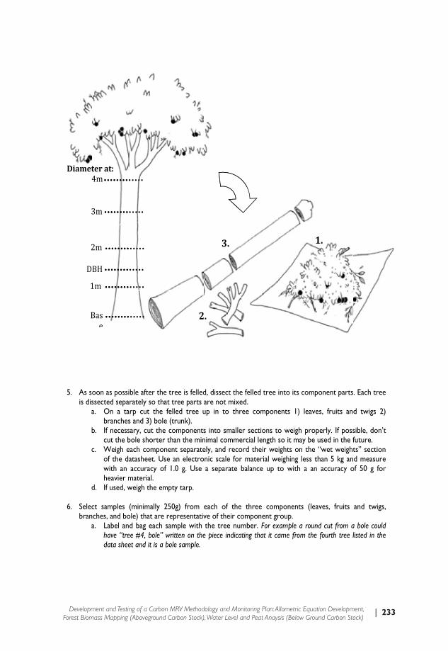
| 233Development and Testing of a Carbon MRV Methodology and Monitoring Plan: Allometric Equation Development, Forest Biomass Mapping (Aboveground Carbon Stock), Water Level and Peat Anaysis (Below Ground Carbon Stock)
5. As sis dis
a
b
c
d
6. Selecbran
a
B
2
1
D
Diamet
3
4
Figure 13.additionalmeasuremweighed in
oon as possissected sepaa. On a ta
branchesb. If necess
cut the bc. Weigh e
of the dawith an heavier m
d. If used, w
ct samples nches, and boa. Label an
have “tredata shee
Base
2m
1m
BH
terat:
3m
4m
Figure 1. Beforel diameter mea
ments are maden sections 1. Le
ble after therately so tha
arp cut the fs and 3) bolesary, cut the bole shorter each componatasheet. Usaccuracy of
material. weigh the em
(minimally 2ole) that are d bag each s
ee #4, bole” wet and it is a b
e the tree is cuasurements are e the bole is cuteaves, fruits and
tree is felledat tree parts felled tree u
e (trunk). componentsthan the min
nent separatee an electro1.0 g. Use
mpty tarp.
250g) from representativsample with written on thebole sample.
2
t diameters aremade in 1 met
t into weighabld twigs, 2. Bran
d, dissect theare not mixeup in to thr
s into smallenimal commeely, and reco
onic scale fora separate
each of theve of their cothe tree num
e piece indica
3.
.
e measured at tter increments e sections, kee
nches, and 3. Bo
e felled tree ied. ree compone
er sections toercial length sord their wer material webalance up t
e three comomponent grmber. For ex
ating that it ca
the base, 1 metalong the bole ping merchantaole.
into its comp
ents 1) leave
o weigh proso it may be ights on the eighing less tto with a an
mponents (leroup. xample a rouname from the
ter, and DBH (1of the tree. Aftable logsif poss
ponent parts
es, fruits an
perly. If possused in the f“wet weigh
than 5 kg ann accuracy o
aves, fruits
nd cut from ae fourth tree l
1.
1.3m). Once theter the diametesible. The entire
s. Each tree
d twigs 2)
sible, don’t future. ts” section
nd measure of 50 g for
and twigs,
a bole could listed in the
e tree is felled er e tree is

234 | Annex 2: Standard OperationProcedure for Allometric Development and Verification
b. For greater trees that are larger than 30 cm DBH, take two samples because the tree will have different wood densities. Take one sample from the base of the tree and a second sample from above the DBH.
c. Weight each sample and record on the datasheet.
7. Repeat steps 4 - 6 above for each of the trees selected in step 1.
Belowground Biomass - Roots (Optional)
Default values from the IPCC GPG LULUCF can be used to quantify belowground biomass for trees, even if the tree was destructively sampled (see section 0). To have more site specific data, roots can be extracted and measured. For every tree felled in the section above, roots and the belowground portion of the stems must extracted and identified by the tree number listed above.
Equipment Needed: • DBH tapes • Linear tape • Weighing scale • Sample collection bags • Chainsaw • Handsaw or other cutting tools • Tarp • Hoes • Shovels
1. Once the trees are cut at ground-level and felled dig up the roots for the trees. a. Start at the stump and collect the roots that originate from the stump. Include belowground
portion of tree stump. b. Dig around the stump as deep as possible and as far away as necessary to collect the tree
roots. c. Collect all the roots to as small as is logistically possible. The more roots collected the
more accurate the data. Recommended smallest root diameter to consider is 10 mm. d. Clean the root to get rid of soil or dust with brush or water.
WATCH OUT! Only collect the roots from the selected tree. Roots from surrounding trees may cross around and under the stump. Only collect roots that originate from the selected stump.
2. The samples will be weighed in three components 1) belowground portion of stump with large
roots, 2) large roots (roots with a diameter of 10 cm or greater) and 3) small roots (roots with a diameter less than 10 cm).
a. On a tarp cut the stump and roots in to three components. b. If necessary, cut the components into smaller sections to weigh properly. c. Weigh each component separately, and record their weights on the “wet weights” section
of the datasheet. Use an electronic scale for material weighing less than 5 kg and measure with an accuracy of 1.0 g. Use a separate balance up to with a an accuracy of 50 g for heavier material.
d. If the samples were weighed in a tarp, weigh the empty tarp.
3. Select samples (minimally 250g) from each of the three components that are representative of their component group.

| 235Development and Testing of a Carbon MRV Methodology and Monitoring Plan: Allometric Equation Development, Forest Biomass Mapping (Aboveground Carbon Stock), Water Level and Peat Anaysis (Below Ground Carbon Stock)
a. Label (and bag if necessary) each sample with the tree number. For example a round cut from a stump could have “tree #4, stump” written on the piece indicating that it came from the fourth tree listed in the data sheet and it is a stump sample.
4. Backfill the hole created by extracting the roots.
5. Limited Measurements
Aboveground Biomass
Biomass from Limited Measurements is calculated by using equations to estimate biomass in tree logs, and factoring in the biomass of the branches, leaves, fruits, and twigs. Many of the limited measurements are made by “visualizing” the log within the tree. Different equations use different measurements along the bole. The procedure below takes all measurements into account, so the equation to be used can be decided at a later date.
Equipment Needed: • DBH tape • Linear tape • Ladder • Weighing scale • Sample collection bags
1. Select and mark at least 10 trees covering the range of DBH existing in the project area (the
minimum DBH should be 5 cm). These trees must be representative of the forest in the project area. When selecting trees take into account species, management, ecological conditions, canopy cover etc. Trees must be tracked using the number on the datasheet, and each sample must be tracked to the same tree number.
2. Measure and record the flowing for every tree: a. Record the tree’s DBH. b. Record the diameter of the tree at the base (ground level). c. Record the diameter at 1 meter intervals along the bole to the top of the bole. d. Record the diameter of the top of the bole at the minimal merchantable diameter. If the top
of the bole is less than 5 cm diameter, record 5 cm, and consider that point the “top of the bole”.
e. Record the height of the bole from the base (point at which b. was measured) to the top of the bole (point at which d. was measured).
f. Record the diameter at the half of the height of the bowl of the tree (divide the height recorded in e. by two to find the half height).
g. Record the tree species.

236 | Annex 2: Standard OperationProcedure for Allometric Development and Verification
Belowg
BelowgrTable3Aavailable
6. Fie
6.1 De
1. All splacethe mor
1. Calc
W
Figure 14
ground Biom
ound biomasA.1.8 when p
i.e., by follow
eld Lab P
estructive
samples muste over many1g accuracy.e than 0.05 g
culate moistu
Where, �����
Diametersmeasuredalongthebole
4. The log on th
mass (Root
ss can be indproject speciwing proced
Procedure
e Sampling
t be dried toy days. Oven. The sampleg.
ure contents
����
=
Base of
Top of
Center of
he right helps “v
ts)
directly estimfic data is nures in sectio
es and Ca
g
o a constant-dry the same has reache
for each sam
�� ������ �
��
f tree
1mDBH
2m
f bole
f bole
6m
5m
4m
3m
visualize” the m
mated by usinnot available.on 0, then su
alculatio
t weight to rmple in the laed a constan
mple of each
���������
∙ 10
Moisture c
measurements
ng the root t. If the projuch data can
ns
remove moisaboratory atnt weight wh
component u
00
content of co
needed for the
to shoot (R:ect specific be used.
sture. Dryingt 70 °C and hen the wei
using the foll
omponent �
Base of tre
Top of the(greater th5 cm diam
Center of b
e limited measu
:S) ratios in Iroot to sho
g the samplerecord theirght does no
lowing formu
[%]
ee
bole han or equameter)
bole
urements.
IPCC-GPG oot data is
es will take r weight to ot fluctuate
ula:
al to
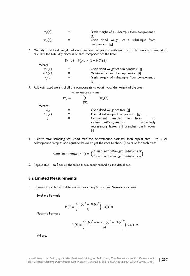
| 237Development and Testing of a Carbon MRV Methodology and Monitoring Plan: Allometric Equation Development, Forest Biomass Mapping (Aboveground Carbon Stock), Water Level and Peat Anaysis (Below Ground Carbon Stock)
����� = Fresh weight of a subsample from component � [g]
����� = Oven dried weight of a subsample from component � [g]
2. Multiply total fresh weight of each biomass component with one minus the moisture content to calculate the total dry biomass of each component of the tree.
����� � ����� ∙ �� � ������ Where,
����� = Oven dried weight of component � [g] ����� = Moisture content of component � [%] ����� = Fresh weight of subsample from component �
[g]
3. Add estimated weight of all the components to obtain total dry weight of the tree.
�� � � ������������������������
���
Where,
�� = Oven dried weight of tree [g]����� = Oven dried sampled component � [g] � = Component sampled i.e. from 1 to
������������������� respectively representing leaves and branches, trunk, roots [-]
4. If destructive sampling was conducted for belowground biomass, then repeat step 1 to 3 for belowground samples and equation below to get the root to shoot (R:S) ratio for each tree:
����� ����� ����� � �� �� � ����� ����� ���������������������� ����� ������������������
�
5. Repeat step 1 to 3 for all the felled trees, enter record on the datasheet.
6.2 Limited Measurements
1. Estimate the volume of different sections using Smalian’sor Newton’s formula.
Smalian’s Formula
���� � ������� � ������
8� ∙ ���� ∙ �
Newton’s Formula
���� � ������� � 4 ∙ ������ � ������
24� ∙ ���� ∙ �
Where,

238 | Annex 2: Standard OperationProcedure for Allometric Development and Verification
����� = Volume of log of section � [m3] ���� = Length of log of section � [m] ����� = Smaller end diameter of log of section � [m] ����� = Middle diameter of log of section � [m] ����� = Larger end diameter of log of section � [m] � = Cut section of cut log from 1, 2, 3, ….to
�������������
2. Add the volume of individual segment to obtain the total volume (V).
�� � � �����������������
���
Where,
�� = Volume of tree [m3] ���� = Volume of log of section � [m3]� = Cut section of cut log from 1, 2, 3, ….to
�������������
3. Multiply by species-specific density (kg m-3) to obtain dry biomass. Use the default value applicable for the species in the region based on IPCC GPG.
�� � �� � �� Where,
�� = Oven dried weight of tree log [g] �� = Volume of tree log [m3] �� = Wood density conversion factor to
converted fresh volume to dried wood. [g m-
3]
4. Add an additional 20 percentage of weight to approximately cover the biomass of branches, leaves, twigs, and fruits.
� � ���� � �� Where,
� = Oven dried weight of tree [g]�� = Volume of tree log [m3]
5. Repeat the step from 1 to 6 for all the selected trees and go to section 5.
7. Equation Verification If the biomass of the measured trees is within ±15% of the mean values predicted by the selected default allometric equation, and is not biased or the bias is towards the conservative side (i.e., equation underestimates of the project net anthropogenic removals by sinks) then mean values predicted from the equation may be used. However, if the If the biomass of the measured trees is not within ±15% of the mean values predicted by the selected default allometric equation, predicted values must be discounted with the relative average half-width of the confidence interval of the model.

| 239Development and Testing of a Carbon MRV Methodology and Monitoring Plan: Allometric Equation Development, Forest Biomass Mapping (Aboveground Carbon Stock), Water Level and Peat Anaysis (Below Ground Carbon Stock)
Weightofemptytarp (kg):___________Thefollowingweightsincludetarpweight 1)Leaves,fruits,twigs 2)Branches 3)Bole
Allometric Equation - Destructive Sampling Datasheet (5+ trees, page 1 of 5)
Time and date of weighing
Tree Component Weight Field measurements:
Leaves, fruits, twigs
Branches Bole
Weight of all felledcomponent in tree (kg):
Weight of wet sample(g) :
In the field laboratory using the compact scale (g): Weight of wet sample:
In the field laboratory using the compact scale afterbaking (g):
Weight of dried sampleafter period 1:
Weight of dried sampleafter period 2:
Weight of dried sampleafter period 3:
Weight of dried sampleafter period 4:
Weight of dried sampleafter period 5:
Weight of dried sampleafter period 6:
Weight of dried sampleafter period 7:
The last weight must match the weight written above it, ± 1g. Each drying period should be about 24 hours.
Project ID Description of forest where tree was found:
SR-Katingan
Species: Height (m): At tree top: At top of bole: DBH (cm):
Diameter at base (cm):
Diameter in cm at: 1 m 2 m 3 m 4 m 5 m 6 m 7 m 8 m 9 m 10 m
11 m 12 m 13 m 14 m 15 m 16 m 17 m 18 m 19 m 20 m
Tree Number:(1, 2, 3, 4 or 5+)
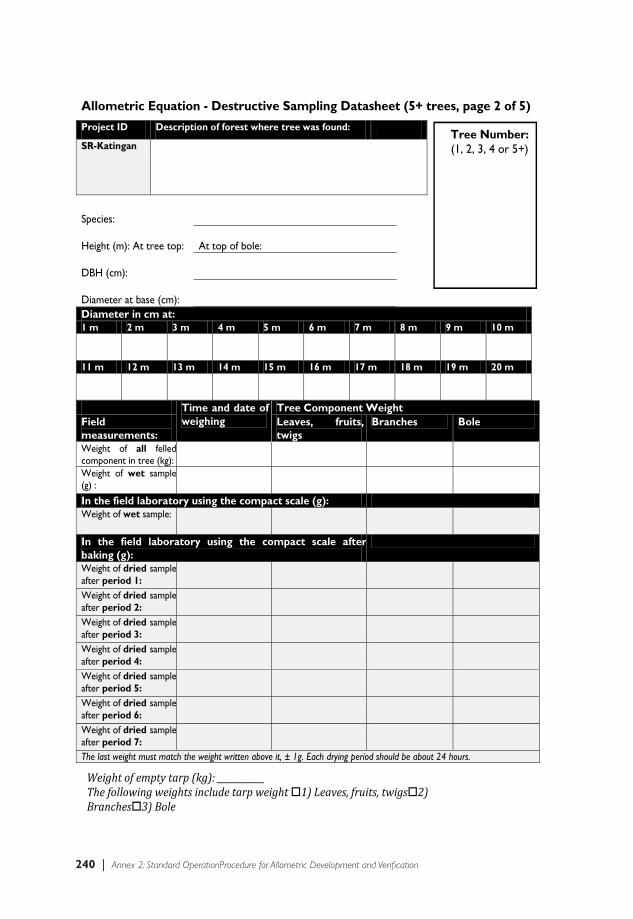
240 | Annex 2: Standard OperationProcedure for Allometric Development and Verification
Weightofemptytarp (kg):___________Thefollowingweightsincludetarpweight 1)Leaves,fruits,twigs 2)Branches 3)Bole
Allometric Equation - Destructive Sampling Datasheet (5+ trees, page 2 of 5)
Time and date of weighing
Tree Component Weight Field measurements:
Leaves, fruits, twigs
Branches Bole
Weight of all felledcomponent in tree (kg):
Weight of wet sample(g) :
In the field laboratory using the compact scale (g): Weight of wet sample:
In the field laboratory using the compact scale afterbaking (g):
Weight of dried sampleafter period 1:
Weight of dried sampleafter period 2:
Weight of dried sampleafter period 3:
Weight of dried sampleafter period 4:
Weight of dried sampleafter period 5:
Weight of dried sampleafter period 6:
Weight of dried sampleafter period 7:
The last weight must match the weight written above it, ± 1g. Each drying period should be about 24 hours.
Project ID Description of forest where tree was found:
SR-Katingan
Species: Height (m): At tree top: At top of bole: DBH (cm):
Diameter at base (cm):
Diameter in cm at: 1 m 2 m 3 m 4 m 5 m 6 m 7 m 8 m 9 m 10 m
11 m 12 m 13 m 14 m 15 m 16 m 17 m 18 m 19 m 20 m
Tree Number:(1, 2, 3, 4 or 5+)

| 241Development and Testing of a Carbon MRV Methodology and Monitoring Plan: Allometric Equation Development, Forest Biomass Mapping (Aboveground Carbon Stock), Water Level and Peat Anaysis (Below Ground Carbon Stock)
Weightofemptytarp (kg):___________Thefollowingweightsincludetarpweight 1)Leaves,fruits,twigs 2)Branches 3)Bole
Allometric Equation - Destructive Sampling Datasheet (5+ trees, page 3 of 5)
Time and date of weighing
Tree Component Weight Field measurements:
Leaves, fruits, twigs
Branches Bole
Weight of all felledcomponent in tree (kg):
Weight of wet sample(g) :
In the field laboratory using the compact scale (g): Weight of wet sample:
In the field laboratory using the compact scale afterbaking (g):
Weight of dried sampleafter period 1:
Weight of dried sampleafter period 2:
Weight of dried sampleafter period 3:
Weight of dried sampleafter period 4:
Weight of dried sampleafter period 5:
Weight of dried sampleafter period 6:
Weight of dried sampleafter period 7:
The last weight must match the weight written above it, ± 1g. Each drying period should be about 24 hours.
Project ID Description of forest where tree was found:
SR-Katingan
Species: Height (m): At tree top: At top of bole: DBH (cm):
Diameter at base (cm):
Diameter in cm at: 1 m 2 m 3 m 4 m 5 m 6 m 7 m 8 m 9 m 10 m
11 m 12 m 13 m 14 m 15 m 16 m 17 m 18 m 19 m 20 m
Tree Number:(1, 2, 3, 4 or 5+)

242 | Annex 2: Standard OperationProcedure for Allometric Development and Verification
Weightofemptytarp (kg):___________Thefollowingweightsincludetarpweight 1)Leaves,fruits,twigs 2)Branches 3)Bole
Allometric Equation - Destructive Sampling Datasheet (5+ trees, page 4 of 5)
Time and date of weighing
Tree Component Weight Field measurements:
Leaves, fruits, twigs
Branches Bole
Weight of all felledcomponent in tree (kg):
Weight of wet sample(g) :
In the field laboratory using the compact scale (g): Weight of wet sample:
In the field laboratory using the compact scale afterbaking (g):
Weight of dried sampleafter period 1:
Weight of dried sampleafter period 2:
Weight of dried sampleafter period 3:
Weight of dried sampleafter period 4:
Weight of dried sampleafter period 5:
Weight of dried sampleafter period 6:
Weight of dried sampleafter period 7:
The last weight must match the weight written above it, ± 1g. Each drying period should be about 24 hours.
Project ID Description of forest where tree was found:
SR-Katingan
Species: Height (m): At tree top: At top of bole: DBH (cm):
Diameter at base (cm):
Diameter in cm at: 1 m 2 m 3 m 4 m 5 m 6 m 7 m 8 m 9 m 10 m
11 m 12 m 13 m 14 m 15 m 16 m 17 m 18 m 19 m 20 m
Tree Number:(1, 2, 3, 4 or 5+)

| 243Development and Testing of a Carbon MRV Methodology and Monitoring Plan: Allometric Equation Development, Forest Biomass Mapping (Aboveground Carbon Stock), Water Level and Peat Anaysis (Below Ground Carbon Stock)
Weight of empty tarp (kg): ___________ The following weights include tarp weight 1) Leaves, fruits, twigs 2) Branches 3) Bole
Allometric Equation - Destructive Sampling Datasheet (5+ trees, page 5 of 5)
Time and date of weighing
Tree Component Weight Field measurements:
Leaves, fruits, twigs
Branches Bole
Weight of all felledcomponent in tree (kg):
Weight of wet sample(g) :
In the field laboratory using the compact scale (g): Weight of wet sample:
In the field laboratory using the compact scale afterbaking (g):
Weight of dried sampleafter period 1:
Weight of dried sampleafter period 2:
Weight of dried sampleafter period 3:
Weight of dried sampleafter period 4:
Weight of dried sampleafter period 5:
Weight of dried sampleafter period 6:
Weight of dried sampleafter period 7:
The last weight must match the weight written above it, ± 1g. Each drying period should be about 24 hours.
Project ID Description of forest where tree was found:
SR-Katingan
Species: Height: At tree top (m): At top of bole: DBH (cm):
Diameter at base (cm):
Diameter in cm at: 1 m 2 m 3 m 4 m 5 m 6 m 7 m 8 m 9 m 10 m
11 m 12 m 13 m 14 m 15 m 16 m 17 m 18 m 19 m 20 m
Tree Number:(1, 2, 3, 4 or 5+)

244 | Annex 2: Standard OperationProcedure for Allometric Development and Verification
Weight of empty tarp (kg): ___________ The following weights include tarp weight 1) Stump 2) Large roots 3) Small roots
Root to Shoot Ratio Verification - Destructive Sampling (5+ trees, page 1of5)
Project ID Description of forest where tree was found:
SR-Katingan
Species: Height (m): At tree top: At top of bole: DBH (cm):
Diameter at base (cm):
Time and date of weighing
Root Component Weight Field measurements:
Belowground portion of Stump
Large Roots Small Roots
Weight of all removedcomponent in roots:
Weight of wet sample:
In the field laboratory using the compact scale: Weight of wet sample:
In the field laboratory using the compact scale afterbaking:
Weight of dried sampleafter period 1:
Weight of dried sampleafter period 2:
Weight of dried sampleafter period 3:
Weight of dried sampleafter period 4:
Weight of dried sampleafter period 5:
Weight of dried sampleafter period 6:
Weight of dried sampleafter period 7:
The last weight must match the weight written above it, ± 1g. Each drying period should be about 24 hours.
Tree Number:(1, 2, 3, 4 or 5+)
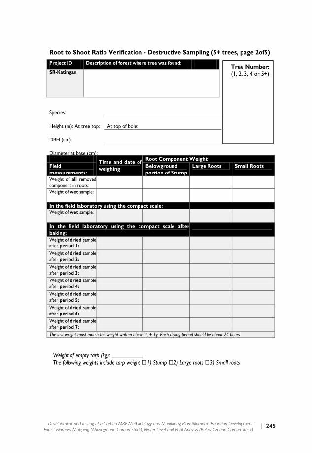
| 245Development and Testing of a Carbon MRV Methodology and Monitoring Plan: Allometric Equation Development, Forest Biomass Mapping (Aboveground Carbon Stock), Water Level and Peat Anaysis (Below Ground Carbon Stock)
Weight of empty tarp (kg): ___________ The following weights include tarp weight 1) Stump 2) Large roots 3) Small roots
Root to Shoot Ratio Verification - Destructive Sampling (5+ trees, page 2of5)
Project ID Description of forest where tree was found:
SR-Katingan
Species: Height (m): At tree top: At top of bole: DBH (cm):
Diameter at base (cm):
Time and date of weighing
Root Component Weight Field measurements:
Belowground portion of Stump
Large Roots Small Roots
Weight of all removedcomponent in roots:
Weight of wet sample:
In the field laboratory using the compact scale: Weight of wet sample:
In the field laboratory using the compact scale afterbaking:
Weight of dried sampleafter period 1:
Weight of dried sampleafter period 2:
Weight of dried sampleafter period 3:
Weight of dried sampleafter period 4:
Weight of dried sampleafter period 5:
Weight of dried sampleafter period 6:
Weight of dried sampleafter period 7:
The last weight must match the weight written above it, ± 1g. Each drying period should be about 24 hours.
Tree Number:(1, 2, 3, 4 or 5+)

246 | Annex 2: Standard OperationProcedure for Allometric Development and Verification
Weight of empty tarp (kg): ___________ The following weights include tarp weight 1) Stump 2) Large roots 3) Small roots
Root to Shoot Ratio Verification - Destructive Sampling (5+ trees, page 3of5)
Project ID Description of forest where tree was found:
SR-Katingan
Species: Height (m): At tree top: At top of bole: DBH (cm):
Diameter at base (cm):
Time and date of weighing
Root Component Weight Field measurements:
Belowground portion of Stump
Large Roots Small Roots
Weight of all removedcomponent in roots:
Weight of wet sample:
In the field laboratory using the compact scale: Weight of wet sample:
In the field laboratory using the compact scale afterbaking:
Weight of dried sampleafter period 1:
Weight of dried sampleafter period 2:
Weight of dried sampleafter period 3:
Weight of dried sampleafter period 4:
Weight of dried sampleafter period 5:
Weight of dried sampleafter period 6:
Weight of dried sampleafter period 7:
The last weight must match the weight written above it, ± 1g. Each drying period should be about 24 hours.
Tree Number:(1, 2, 3, 4 or 5+)

| 247Development and Testing of a Carbon MRV Methodology and Monitoring Plan: Allometric Equation Development, Forest Biomass Mapping (Aboveground Carbon Stock), Water Level and Peat Anaysis (Below Ground Carbon Stock)
Weight of empty tarp (kg): ___________ The following weights include tarp weight 1) Stump 2) Large roots 3) Small roots
Root to Shoot Ratio Verification - Destructive Sampling (5+ trees, page 4of5)
Project ID Description of forest where tree was found:
SR-Katingan
Species: Height (m): At tree top: At top of bole: DBH (cm):
Diameter at base (cm):
Time and date of weighing
Root Component Weight Field measurements:
Belowground portion of Stump
Large Roots Small Roots
Weight of all removedcomponent in roots:
Weight of wet sample:
In the field laboratory using the compact scale: Weight of wet sample:
In the field laboratory using the compact scale afterbaking:
Weight of dried sampleafter period 1:
Weight of dried sampleafter period 2:
Weight of dried sampleafter period 3:
Weight of dried sampleafter period 4:
Weight of dried sampleafter period 5:
Weight of dried sampleafter period 6:
Weight of dried sampleafter period 7:
The last weight must match the weight written above it, ± 1g. Each drying period should be about 24 hours.
Tree Number:(1, 2, 3, 4 or 5+)
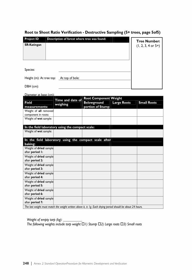
248 | Annex 2: Standard OperationProcedure for Allometric Development and Verification
Weight of empty tarp (kg): ___________ The following weights include tarp weight 1) Stump 2) Large roots 3) Small roots
Root to Shoot Ratio Verification - Destructive Sampling (5+ trees, page 5of5)
Project ID Description of forest where tree was found:
SR-Katingan
Species: Height (m): At tree top: At top of bole: DBH (cm):
Diameter at base (cm):
Time and date of weighing
Root Component Weight Field measurements:
Belowground portion of Stump
Large Roots Small Roots
Weight of all removedcomponent in roots:
Weight of wet sample:
In the field laboratory using the compact scale: Weight of wet sample:
In the field laboratory using the compact scale afterbaking:
Weight of dried sampleafter period 1:
Weight of dried sampleafter period 2:
Weight of dried sampleafter period 3:
Weight of dried sampleafter period 4:
Weight of dried sampleafter period 5:
Weight of dried sampleafter period 6:
Weight of dried sampleafter period 7:
The last weight must match the weight written above it, ± 1g. Each drying period should be about 24 hours.
Tree Number:(1, 2, 3, 4 or 5+)

| 249Development and Testing of a Carbon MRV Methodology and Monitoring Plan: Allometric Equation Development, Forest Biomass Mapping (Aboveground Carbon Stock), Water Level and Peat Anaysis (Below Ground Carbon Stock)
Allometric Equation – Limited Measurements Datasheet (10+ trees, page 1 of 2)
Tree 1 Tree 2 Tree 3 Tree 4 Tree 5
Species:
Height:
Diameter at:
Base
DBH
Center
Top
1 m
2 m
3 m
4 m
5 m
6 m
7 m
8 m
9 m
10 m
Project ID Description of forest where trees were found:
SR-Katingan

250 | Annex 2: Standard OperationProcedure for Allometric Development and Verification
Allometric Equation – Limited Measurements Datasheet (10+ trees, page 2 of 2)
Tree 6 Tree 7 Tree 8 Tree 9 Tree 10
Species:
Height:
Diameter at:
Base
DBH
Center
Top
1 m
2 m
3 m
4 m
5 m
6 m
7 m
8 m
9 m
10 m
Project ID Description of forest where trees were found:
SR-Katingan
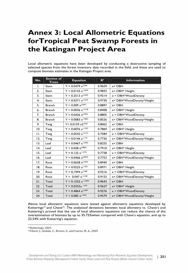
| 251Development and Testing of a Carbon MRV Methodology and Monitoring Plan: Allometric Equation Development, Forest Biomass Mapping (Aboveground Carbon Stock), Water Level and Peat Anaysis (Below Ground Carbon Stock)
Annex 3: Local Allometric Equations forTropical Peat Swamp Forests in the Katingan Project Area Local allometric equations have been developed by conducting a destructive sampling of selected species from the forest inventory data recorded in the field, and these are used to compute biomass estimates in the Katingan Project area.
No. Section of Trees Equation R2 Information
1. Stem Y = 0.0479 x2.604 0.9659 x= DBH
2. Stem Y = 0.0143 x1.5694 0.9833 x= DBH* Height
3. Stem Y = 0.2513 x2.4043 0.9214 x = DBH*WoodDensity
4. Stem Y = 0.0371 x1.5232 0.9730 x= DBH*WoodDensity*Height
5. Branch Y = 0.009 x2.6051 0.8897 x= DBH
6. Branch Y = 0.0036 x1.5128 0.8408 x= DBH* Height
7. Branch Y = 0.0426 x2.4501 0.8805 x = DBH*WoodDensity
8. Branch Y = 0.0083 x1.4864 0.8526 x= DBH*WoodDensity*Height
9. Twig Y= 0.0159 x2.0367 0.8062 x= DBH
10. Twig Y = 0.0076 x1.1937 0.7869 x= DBH* Height
11. Twig Y = 0.0542 x1.9173 0.7584 x = DBH*WoodDensity
12. Twig Y = 0.0146 x1.174 0.7736 x= DBH*WoodDensity*Height
13. Leaf Y = 0.0467 x1.5055 0.8255 x= DBH
14. Leaf Y = 0.028 x0.8803 0.7910 x= DBH* Height
15. Leaf Y = 0.125 x1.3779 0.7738 x = DBH*WoodDensity
16. Leaf Y = 0.0466 x0.8503 0.7753 x= DBH*WoodDensity*Height
17. Root Y = 0.0628 x2.0565 0.8940 x= DBH
18. Root Y = 0.0225 x1.2501 0.8971 x= DBH* Height
19. Root Y = 0,1994 x1.968 0.9216 x = DBH*WoodDensity
20. Root Y = 0.047 x1.2184 0.9153 x= DBH*WoodDensity*Height
21. Total Y = 0.1032 x 2.4695 0.9643 x= DBH
22. Total Y = 0.0355x 1.474 0.9627 x= DBH* Height
23. Total Y = 0.4864 x2.2897 0.9276 x = DBH*WoodDensity
24. Total Y = 0.085 x1.4345 0.9579 x= DBH*WoodDensity*Height
Above local allometric equations were tested against allometric equations developed by Ketterings15 and Chave16. The analysisof deviations between local allometry vs. Chave’s and Kettering’s proved that the use of local allometric equations can reduce the chance of the overestimation of biomass by up to 35.72%when compared with Chave’s equation, and up to 22.54% with Kettering’s equation. 15Ketterings, 2001. 16Chave, J., Andalo, C., Brown, S., and Cairns, M. A., 2005

252 | Annex 3: Local Allometric Equations forTropical Peat Swamp Forests in the Katingan Project Area

| 253Development and Testing of a Carbon MRV Methodology and Monitoring Plan: Allometric Equation Development, Forest Biomass Mapping (Aboveground Carbon Stock), Water Level and Peat Anaysis (Below Ground Carbon Stock)
Annex 4: Aboveground and Belowground Carbon Stock Estimation for the Katingan Project Area 1. Total carbon stock estimation The total carbon stocks of both aboveground and belowground biomass in primary forest, logged-over forest and ex-burnt forest were estimatedas indicated in Table 1 and Figure 1. Table 1. Estimated total Carbon Stocks for different forest types
Forest Type Carbon Pools Carbon Stock
(ton/ha) Ex-Burnt Secondary Forest
Stand (above & belowground-root) 24.54Understorey 14.52Litter 12.28Necromass 6.22Peat 596.80Total 654.36
Logged-over Secondary Forest
Stand (above & belowground-root) 51.01Understorey 6.83Litter 16.89Necromass 2.72Peat 3103.50Total 3180.93
Primary Forest Stand (above & belowground-root) 101.90Understorey 6.15Litter 17.99Necromass 3.22Peat 3295.09Total 3424.36
Carbonstock estimationwas obtained from theconversion ofbiomassmultiplied by thepercentage of carbon fraction in each plant part, which wasderivedfromthe results oflaboratoryanalysis.
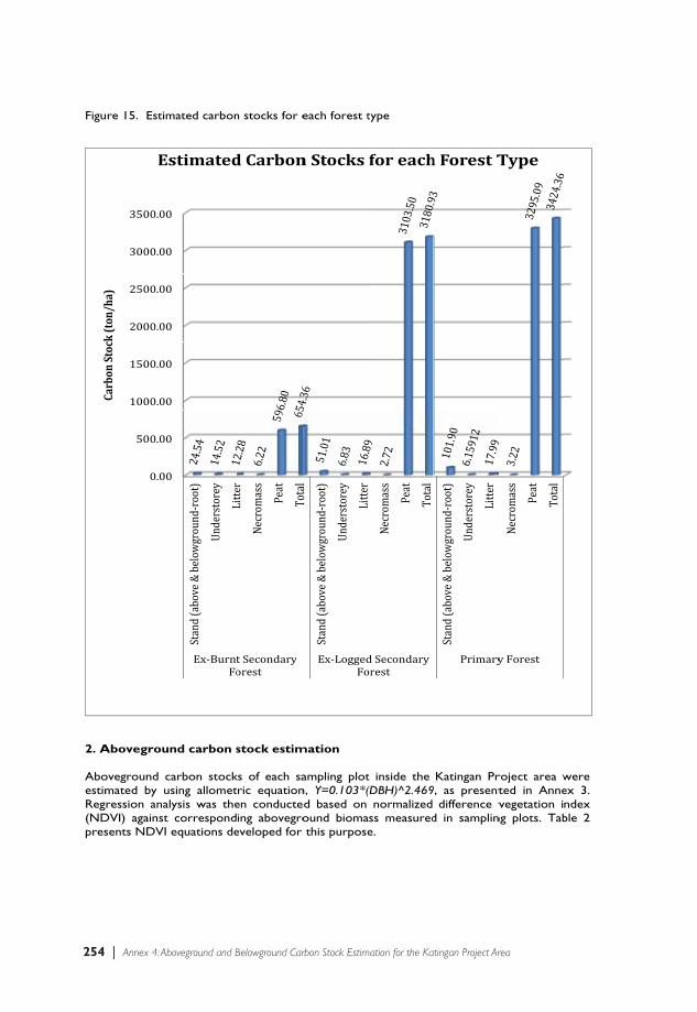
254 | Annex 4: Aboveground and Belowground Carbon Stock Estimation for the Katingan Project Area
Figu
2. A AboestimRegr(NDpres
Carbon
Stock(ton/ha)
re 15. Estim
Abovegroun
oveground camated by usression analy
DVI) against sents NDVI e
0.00
500.00
1000.00
1500.00
2000.00
2500.00
3000.00
3500.00
CarbonStock(ton/ha)
Es
mated carbon
nd carbon s
arbon stocksing allometysis was thecorrespondequations de
Stand (above & below
ground‐ro
ot)
Understorey
Litter
Ex‐BurntFo
stimated
n stocks for e
stock estim
ks of each saric equationen conducteing abovegro
eveloped for
Litter
Necrom
ass
Peat
Total
t Secondaryorest
dCarbon
each forest t
mation
ampling plotn, Y=0.103*(ed based on ound biomathis purpose
Total
Stand (above & below
ground‐ro
ot)
Understorey
Litter
Ex‐LoggedFo
nStocks
type
t inside the (DBH)^2.469
normalized ass measurede.
Necrom
ass
Peat
Total
d Secondaryorest
foreach
Katingan Pr9, as present
difference vd in samplin
Stand (above & below
ground‐ro
ot)
Understorey
Litter
Primary
hForestT
roject area wted in Annevegetation i
ng plots. Tab
Necrom
ass
Peat
Total
y Forest
Type
were ex 3. ndex ble 2

| 255Development and Testing of a Carbon MRV Methodology and Monitoring Plan: Allometric Equation Development, Forest Biomass Mapping (Aboveground Carbon Stock), Water Level and Peat Anaysis (Below Ground Carbon Stock)
Tabl
Prim
Low
Seco The secoLandbiom Figu
17Theimpo
le 2. Aboveg
Forest tymary peat for
w pole primar
ondary peat
carbon maondary foresdsat Thematmass with the
re 2. Carbo
e limitation inortant factor af
ground biom
ype
rest
ry forest
forest
p of the thrt (including btic Mapper (e carbon frac
on map of the
n spatial, spectrffecting the abo
ass equation
AGB = 5189
AGB = -960
AGB = 1986
ree forest tyboth logged-(TM) 517 andction of 45%
e Katingan P
ral, and radiomoveground bio
ns for NDVI
AGB e91 (NDVI)2 –
05.1(NDVI)2
6.4(NDVI)2 -
ypes – prim-over and exd multiplying% (see Figure
Project area
metric resolutiomass estimati
regression a
equation
– 61531 (ND
+ 10165 (N
- 2643.7 (ND
ary forest, lx-burnt foresg the amoun
2).
ions inherent ion performan
nalysis
DVI) + 18386
DVI) - 2542.
DVI) + 972.9
ow pole prists) – was get of estimat
in the remotelce.
R2 6 0.7265
.4 0.6571
91 0.6553
imary forestenerated by uted abovegro
ly sensed data
t and using ound
a is an
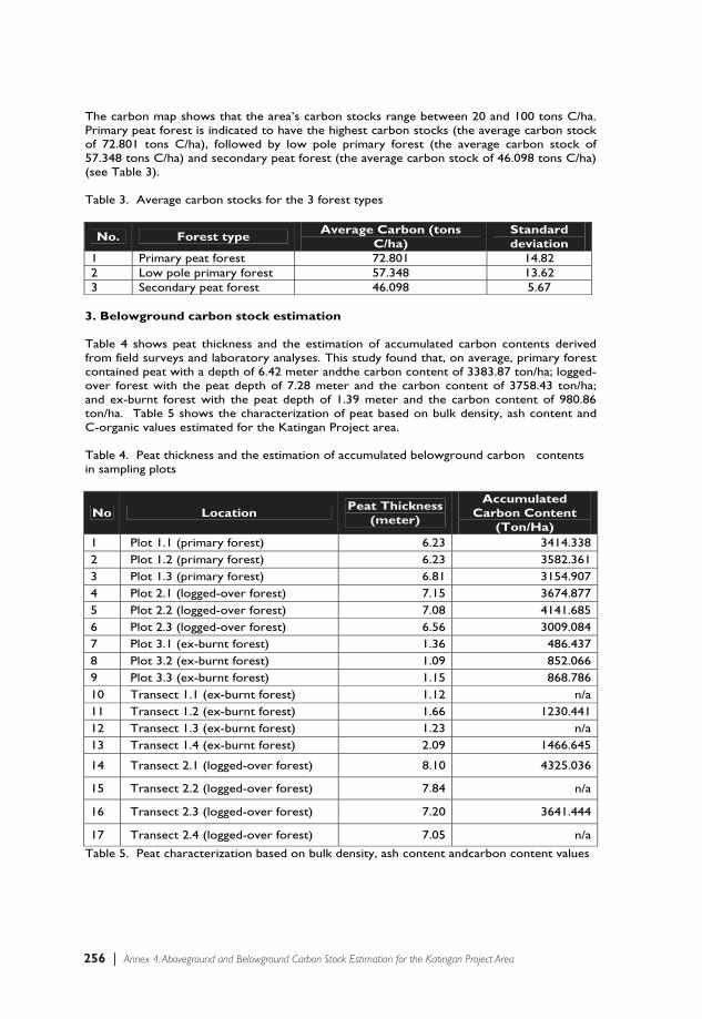
256 | Annex 4: Aboveground and Belowground Carbon Stock Estimation for the Katingan Project Area
The carbon map shows that the area’s carbon stocks range between 20 and 100 tons C/ha. Primary peat forest is indicated to have the highest carbon stocks (the average carbon stock of 72.801 tons C/ha), followed by low pole primary forest (the average carbon stock of 57.348 tons C/ha) and secondary peat forest (the average carbon stock of 46.098 tons C/ha) (see Table 3). Table 3. Average carbon stocks for the 3 forest types
No. Forest type Average Carbon (tons
C/ha) Standard deviation
1 Primary peat forest 72.801 14.82 2 Low pole primary forest 57.348 13.62 3 Secondary peat forest 46.098 5.67
3. Belowground carbon stock estimation Table 4 shows peat thickness and the estimation of accumulated carbon contents derived from field surveys and laboratory analyses. This study found that, on average, primary forest contained peat with a depth of 6.42 meter andthe carbon content of 3383.87 ton/ha; logged-over forest with the peat depth of 7.28 meter and the carbon content of 3758.43 ton/ha; and ex-burnt forest with the peat depth of 1.39 meter and the carbon content of 980.86 ton/ha. Table 5 shows the characterization of peat based on bulk density, ash content and C-organic values estimated for the Katingan Project area. Table 4. Peat thickness and the estimation of accumulated belowground carbon contents in sampling plots
No Location Peat Thickness
(meter)
Accumulated Carbon Content
(Ton/Ha) 1 Plot 1.1 (primary forest) 6.23 3414.3382 Plot 1.2 (primary forest) 6.23 3582.3613 Plot 1.3 (primary forest) 6.81 3154.9074 Plot 2.1 (logged-over forest) 7.15 3674.8775 Plot 2.2 (logged-over forest) 7.08 4141.6856 Plot 2.3 (logged-over forest) 6.56 3009.0847 Plot 3.1 (ex-burnt forest) 1.36 486.4378 Plot 3.2 (ex-burnt forest) 1.09 852.0669 Plot 3.3 (ex-burnt forest) 1.15 868.78610 Transect 1.1 (ex-burnt forest) 1.12 n/a11 Transect 1.2 (ex-burnt forest) 1.66 1230.44112 Transect 1.3 (ex-burnt forest) 1.23 n/a13 Transect 1.4 (ex-burnt forest) 2.09 1466.645
14 Transect 2.1 (logged-over forest) 8.10 4325.036
15 Transect 2.2 (logged-over forest) 7.84 n/a
16 Transect 2.3 (logged-over forest) 7.20 3641.444
17 Transect 2.4 (logged-over forest) 7.05 n/a
Table 5. Peat characterization based on bulk density, ash content andcarbon content values
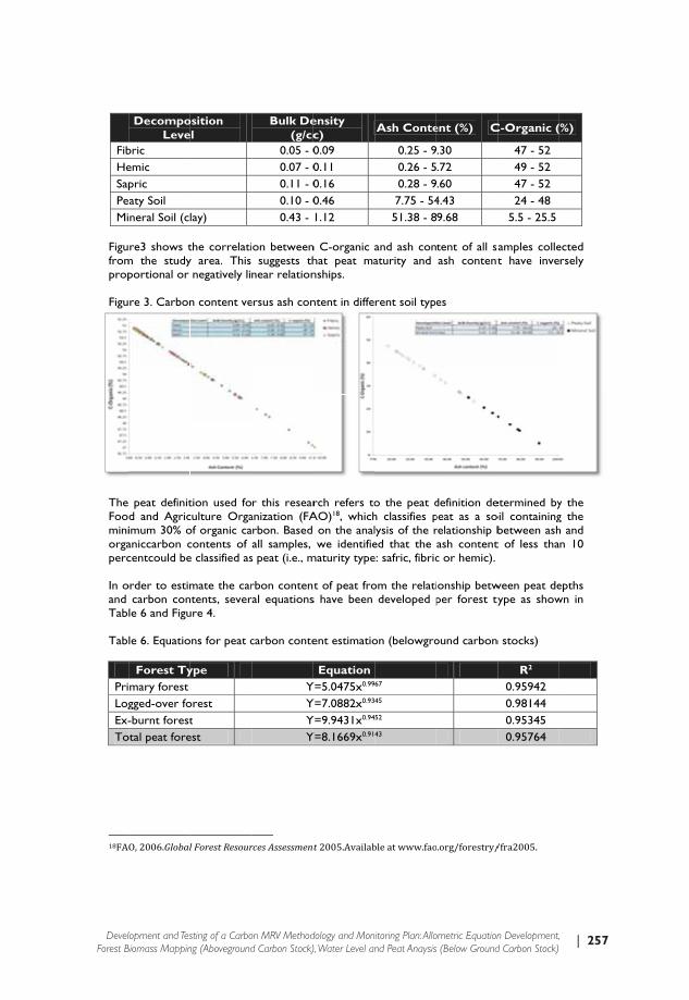
| 257Development and Testing of a Carbon MRV Methodology and Monitoring Plan: Allometric Equation Development, Forest Biomass Mapping (Aboveground Carbon Stock), Water Level and Peat Anaysis (Below Ground Carbon Stock)
FibHeSapPeMi
Figufromprop Figu
The Foominiorgaperc In oand Tabl Tabl
PriLogEx-To
18FAO
DecompoLeve
bric emic pric aty Soil neral Soil (cl
re3 shows t
m the studyportional or
re 3. Carbon
peat definitd and Agricimum 30% oaniccarbon ccentcould be
order to estimcarbon con
le 6 and Figu
le 6. Equatio
Forest Tymary forest gged-over fo-burnt forest
otal peat fore
O, 2006.Global
osition el
lay)
the correlatiy area. This negatively li
n content ve
tion used foculture Orgaof organic cacontents of e classified as
mate the carntents, severure 4.
ons for peat c
ype
orest t est
lForestResour
Bulk De(g/cc
0.05 - 00.07 - 00.11 - 00.10 - 00.43 -
on betweensuggests th
near relation
ersus ash con
r this researanization (FArbon. Based all samples,
s peat (i.e., m
rbon contenral equations
carbon conte
YYYY
rcesAssessmen
ensity c) 0.09 0.11 0.16 0.46 1.12
n C-organic ahat peat manships.
ntent in diffe
rch refers toAO)18, which on the analwe identifie
maturity type
t of peat fros have been
ent estimatio
EquationY=5.0475x0.99
Y=7.0882x0.93
Y=9.9431x0.94
Y=8.1669x0.91
t 2005.Availab
Ash Conte
0.25 - 90.26 - 50.28 - 97.75 - 5451.38 - 8
and ash conaturity and
rent soil typ
o the peat dh classifies plysis of the red that the e: safric, fibric
om the relatideveloped p
on (belowgro
67 45 52 43
ble at www.fao
ent (%) C
.30
.72
.60 4.43 9.68
tent of all saash content
es
definition depeat as a sorelationship bash contentc or hemic).
ionship betwper forest ty
ound carbon
o.org/forestry/
C-Organic (
47 - 52 49 - 52 47 - 52 24 - 48
5.5 - 25.5
amples collet have inve
etermined byoil containingbetween asht of less tha
ween peat deype as show
n stocks)
R2 0.95942 0.98144 0.95345 0.95764
/fra2005.
(%)
ected rsely
y the g the h and n 10
epths wn in
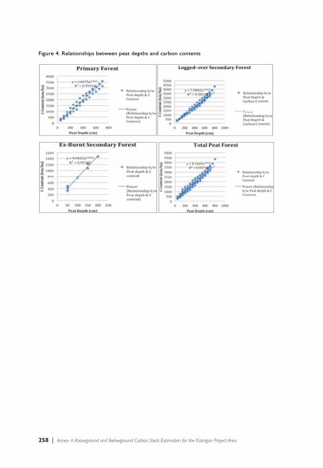
258 | Annex 4: Aboveground and Belowground Carbon Stock Estimation for the Katingan Project Area
Figu
re 4. Relatio
onships betwween peat deppths and carbon contentts

| 259Development and Testing of a Carbon MRV Methodology and Monitoring Plan: Allometric Equation Development, Forest Biomass Mapping (Aboveground Carbon Stock), Water Level and Peat Anaysis (Below Ground Carbon Stock)
An
nex
5: E
nvi
ronm
enta
l Saf
egu
ard
Str
ateg
ies
for
HC
V A
reas
in t
heK
atin
gan
Pro
ject
are
a
HC
V
Att
rib
ute
T
hre
ats
Man
agem
ent
Ob
ject
ives
P
rim
ary
Man
agem
ent
Str
ateg
y(s)
1.
1 A
reas
tha
t co
ntai
n or
pr
ovid
e bi
odiv
ersi
ty
supp
ort
func
tions
to
prot
ectio
n or
co
nser
vatio
n ar
eas
1)co
nver
sion
of
area
func
tion
espe
cial
ly t
he o
ne lo
cate
d al
ong
the
rive
r/ca
nal f
or
agri
cultu
re, g
arde
n an
d ot
her
land
use
; 2)
coal
and
gol
d m
inin
g;
3)pe
at d
rain
age;
4)
illeg
al lo
ggin
g 5)
fore
st fi
re/fi
re t
o op
en n
ew
area
s
Mon
itori
ng o
f for
est
cove
r ch
ange
cou
ld b
e us
ed a
s on
e of
the
impo
rtan
t st
rate
gy t
o m
anag
e th
e co
nces
sion
are
a as
a p
reca
utio
n st
ep t
o an
ticip
ate
exte
rnal
dis
turb
ance
s th
at m
ight
be
elev
ate.
T
here
fore
, the
miti
gatio
n of
ext
erna
l dis
turb
ance
s w
ould
be
easy
so
that
eco
syst
em fu
nctio
n st
abili
ty
and
mai
ntai
ning
the
via
ble
popu
latio
n of
impo
rtan
t sp
ecie
s in
the
are
a of
PT
. RM
U c
ould
be
achi
eved
.
1)Fo
rest
Pro
tect
ion
Stra
tegy
;
2)C
olla
bora
tive
Biod
iver
sity
M
anag
emen
t St
rate
gy; a
nd
3)
Fore
st R
esto
ratio
n St
rate
gy
1.2
Cri
tical
ly E
ndan
gere
d Sp
ecie
s 1)
conv
ersi
on o
f ar
ea fu
nctio
n es
peci
ally
the
one
loca
ted
alon
g th
e ri
ver/
cana
l for
ag
ricu
lture
, gar
den
and
othe
r la
nd u
se;
2)pe
at d
rain
age;
3)
illeg
al lo
ggin
g; a
nd
4)fo
rest
fire
and
use
s of
fire
for
open
ing
new
land
1)m
onito
ring
CR
spe
cies
of b
oth
flora
l and
fa
unal
by
carr
ying
out
sur
vey
in s
ever
al p
lace
s in
side
con
cess
ion
area
to
obse
rve
and
exam
ine
of it
s po
pula
tion
2)m
itiga
tion
of il
lega
l log
ging
insi
de c
once
ssio
n ar
ea
3)re
stor
ing
or m
aint
aini
ng n
atur
al r
egen
erat
ion
of C
R s
peci
es o
f pla
nt t
hat
grow
s in
man
y pl
aces
of f
ores
t m
anag
emen
t un
it
4)us
ing
GIS
and
Rem
ote
Sens
ing
soft
war
e sy
stem
to
mon
itor
fore
st c
over
cha
nge
to
antic
ipat
e an
d ea
sily
miti
gate
ext
erna
l di
stur
banc
es in
ord
er t
o m
aint
ain
over
all
ecos
yste
m fu
nctio
n st
abili
ty
1)Fo
rest
Pro
tect
ion
Stra
tegy
;
2)C
olla
bora
tive
Biod
iver
sity
M
anag
emen
t St
rate
gy;
3)
In-s
itu C
onse
rvat
ion
Stra
tegy
; and
4)Fo
rest
Res
tora
tion
Stra
tegy
1.3
Are
as t
hat
cont
ain
Hab
itat
for
Via
ble
1)co
nver
sion
of
area
func
tion
espe
cial
ly t
he o
ne lo
cate
d 1)
m
onito
ring
of b
oth
flora
and
faun
a of
HC
V 1
.3
by c
arry
ing
out
surv
ey t
o m
ap t
he d
istr
ibut
ion
1)Fo
rest
Pro
tect
ion
Stra
tegy
;

260 | Annex 5: Environmental afeguard Strategies for HCV Areas in the Katingan Project area
HC
V
Att
rib
ute
T
hre
ats
Man
agem
ent
Ob
ject
ives
P
rim
ary
Man
agem
ent
Str
ateg
y(s)
Po
pula
tions
of
Enda
nger
ed, R
estr
icte
d R
ange
or
Prot
ecte
d Sp
ecie
s
alon
g th
e ri
ver/
cana
l for
ag
ricu
lture
, gar
den
and
othe
r la
nd u
se;
2)pe
at d
rain
age;
3)
illeg
al lo
ggin
g;
4)fo
rest
fire
and
use
s of
fire
for
open
ing
new
land
; and
5)
hunt
ing
and
exam
ine
its p
opul
atio
n 2)
m
inim
ize
hunt
ing
and
illeg
al lo
ggin
g in
side
the
co
nces
sion
of P
T. R
MU
; 3)
re
stor
ing
and
mai
ntai
ning
nat
ural
reg
ener
atio
n of
HC
V 1
.3 s
peci
es t
hat
grow
s at
fore
st
man
agem
ent
unit;
4)
us
ing
GIS
and
Rem
ote
Sens
ing
soft
war
e sy
stem
to
mon
itor
fore
st c
over
cha
nge
to
antic
ipat
e an
d ea
sily
miti
gate
ext
erna
l di
stur
banc
es in
ord
er t
o m
aint
ain
over
all
ecos
yste
m fu
nctio
n st
abili
ty
2)C
olla
bora
tive
Biod
iver
sity
M
anag
emen
t St
rate
gy;
3)Ex
-situ
and
In-s
itu
Con
serv
atio
n St
rate
gy; a
nd
4)Fo
rest
Res
tora
tion
Stra
tegy
1.4
Spec
ific
Hab
itats
tha
t ar
e U
sed
Tem
pora
rily
by
a S
peci
es o
r G
roup
of
Spe
cies
1)co
nver
sion
of
area
func
tion
espe
cial
ly t
he o
ne lo
cate
d al
ong
the
rive
r/ca
nal f
or
agri
cultu
re, g
arde
n an
d ot
her
land
use
; 2)
peat
dra
inag
e;
3)ill
egal
logg
ing;
4)
fore
st fi
re a
nd u
ses
of fi
re fo
r op
enin
g ne
w la
nd; a
nd
5)hu
ntin
g
1)
cond
uctin
g su
rvey
to
map
the
dis
trib
utio
n of
th
e sp
ecie
s an
d to
mon
itor
the
popu
latio
n of
m
igra
nt b
irds
insi
de a
nd a
roun
d PT
. RM
U
conc
essi
on;
2)
usin
g G
IS a
nd R
emot
e Se
nsin
g so
ftw
are
syst
em t
o m
onito
r fo
rest
cov
er c
hang
e to
an
ticip
ate
and
easi
ly m
itiga
te e
xter
nal
dist
urba
nces
in o
rder
to
mai
ntai
n ov
eral
l ec
osys
tem
func
tion
stab
ility
1)Fo
rest
Pro
tect
ion
Stra
tegy
; 2)
Col
labo
rativ
e Bi
odiv
ersi
ty
Man
agem
ent
Stra
tegy
;
2.1
Larg
e N
atur
al
Land
scap
es w
ith t
he
Cap
acity
to
Mai
ntai
n N
atur
al E
colo
gica
l Pr
oces
ses
and
Dyn
amic
s
1)co
nver
sion
of
area
func
tion
espe
cial
ly t
he o
ne lo
cate
d al
ong
the
rive
r/ca
nal f
or
agri
cultu
re, g
arde
n an
d ot
her
land
use
; 2)
peat
dra
inag
e;
3)ill
egal
logg
ing;
and
4)
fore
st fi
re a
nd u
ses
of fi
re fo
r op
enin
g ne
w la
nd
Mon
itori
ng o
f for
est
cove
r ch
ange
con
side
red
an
impo
rtan
t to
man
age
the
conc
essi
on a
rea
as a
pr
ecau
tion
step
to
antic
ipat
e ex
tern
al d
istu
rban
ces
that
mig
ht b
e ra
ise.
The
refo
re, t
he m
itiga
tion
of
exte
rnal
dis
turb
ance
s w
ould
be
easy
so
that
the
co
re a
rea
of p
eat
swam
p ec
osys
tem
in t
he
conc
essi
on a
rea
of P
T. R
MU
cou
ld b
e m
aint
aine
d.
1)Fo
rest
Pro
tect
ion
Stra
tegy
; 2)
Col
labo
rativ
e Bi
odiv
ersi
ty
Man
agem
ent
Stra
tegy
; and
3)
Fore
st R
esto
ratio
n St
rate
gy
2.2
Are
as t
hat
Con
tain
Tw
o or
Mor
e C
ontig
uous
Ec
osys
tem
1)co
nver
sion
of
area
func
tion
espe
cial
ly t
he o
ne lo
cate
d al
ong
the
rive
r/ca
nal f
or
agri
cultu
re, g
arde
n an
d ot
her
Mon
itori
ng o
f for
est
cove
r ch
ange
con
side
red
an
impo
rtan
t st
rate
gy t
o m
anag
e th
e co
nces
sion
are
a as
a p
reca
utio
n st
ep t
o an
ticip
ate
exte
rnal
di
stur
banc
es t
hat
mig
ht b
e ra
ised
. T
here
fore
, the
1)Fo
rest
Pro
tect
ion
Stra
tegy
; 2)
Col
labo
rativ
e Bi
odiv
ersi
ty
Man
agem
ent
Stra
tegy
; and

| 261Development and Testing of a Carbon MRV Methodology and Monitoring Plan: Allometric Equation Development, Forest Biomass Mapping (Aboveground Carbon Stock), Water Level and Peat Anaysis (Below Ground Carbon Stock)
HC
V
Att
ribu
te
Th
reat
s M
anag
emen
t O
bje
ctiv
es
Pri
mar
y M
anag
emen
t S
trat
egy(
s)
land
use
; 2)
peat
dra
inag
e;
3)ill
egal
logg
ing;
and
4)
fore
st fi
re a
nd u
ses
of fi
re fo
r op
enin
g ne
w la
nd
miti
gatio
n of
ext
erna
l dis
turb
ance
s w
ould
be
easy
so
tha
t th
e ov
eral
l con
tinuo
us e
cosy
stem
cou
ld b
e m
aint
aine
d.
3)Fo
rest
Res
tora
tion
Stra
tegy
2.3
Are
as t
hat
Con
tain
R
epre
sent
ativ
e Po
pula
tions
of M
ost
Nat
ural
ly O
ccur
ring
Sp
ecie
s
1)co
nver
sion
of
area
func
tion
espe
cial
ly t
he o
ne lo
cate
d al
ong
the
rive
r/ca
nal f
or
agri
cultu
re, g
arde
n an
d ot
her
land
use
; 2)
peat
dra
inag
e;
3)ill
egal
logg
ing;
4)
fore
st fi
re a
nd u
ses
of fi
re fo
r op
enin
g ne
w la
nd; a
nd
5)hu
ntin
g
1)
mon
itori
ng o
f bot
h flo
ra a
nd fa
una
of H
CV
1.2
an
d H
CV
1.3
by
carr
ying
out
sur
vey
to m
ap
the
dist
ribu
tion
and
exam
ine
its p
opul
atio
n.
2)
min
imiz
e hu
ntin
g an
d ill
egal
logg
ing
insi
de t
he
conc
essi
on o
f PT
. RM
U;
3)
rest
orin
g an
d m
aint
aini
ng n
atur
al r
egen
erat
ion
of H
CV
1.3
spe
cies
tha
t gr
ows
at fo
rest
m
anag
emen
t un
it;
4)
usin
g G
IS a
nd R
emot
e Se
nsin
g so
ftw
are
syst
em t
o m
onito
r fo
rest
cov
er c
hang
e to
an
ticip
ate
and
easi
ly m
itiga
te e
xter
nal
dist
urba
nces
in o
rder
to
mai
ntai
n ov
eral
l ec
osys
tem
func
tion
stab
ility
.
1)Fo
rest
Pro
tect
ion
Stra
tegy
; 2)
Col
labo
rativ
e Bi
odiv
ersi
ty
Man
agem
ent
Stra
tegy
; 3)
Ex-s
itu a
nd In
-situ
C
onse
rvat
ion
Stra
tegy
; and
4)
Fore
st R
esto
ratio
n St
rate
gy
3 R
are
or E
ndan
gere
d Ec
osys
tem
s 1)
co
nver
sion
of
area
func
tion
espe
cial
ly t
he o
ne lo
cate
d al
ong
the
rive
r/ca
nal f
or
agri
cultu
re, g
arde
n an
d ot
her
land
use
; 2)
co
al a
nd g
old
min
ing;
3)
pe
at d
rain
age;
4)
ill
egal
logg
ing
5)
fore
st fi
re/fi
re t
o op
en n
ew
area
s
Mon
itori
ng o
f for
est
cove
r ch
ange
con
side
red
an
impo
rtan
t st
rate
gy t
o m
anag
e th
e co
nces
sion
are
a as
a p
reca
utio
n st
ep t
o an
ticip
ate
exte
rnal
di
stur
banc
es t
hat
mig
ht b
e ra
ise.
The
refo
re, t
he
miti
gatio
n of
ext
erna
l dis
turb
ance
s w
ould
be
easy
so
tha
t en
dang
ered
eco
syst
em t
ype
in P
T. R
MU
co
nces
sion
esp
ecia
lly w
ith s
mal
l acr
eage
cou
ld b
e m
aint
aine
d.
1)Fo
rest
Pro
tect
ion
Stra
tegy
; 2)
Col
labo
rativ
e Bi
odiv
ersi
ty
Man
agem
ent
Stra
tegy
; and
3)
Fore
st R
esto
ratio
n St
rate
gy
4.1
Are
as o
r Ec
osys
tem
s Im
port
ant
for
the
Prov
isio
n of
Wat
er a
nd
Prev
entio
n of
Flo
ods
for
Dow
nstr
eam
C
omm
uniti
es
1)co
nver
sion
of
area
func
tion
espe
cial
ly t
he o
ne lo
cate
d al
ong
the
rive
r/ca
nal f
or
agri
cultu
re, g
arde
n an
d ot
her
land
use
; 2)
coal
and
gol
d m
inin
g;
Mon
itori
ng o
f for
est
cove
r ch
ange
con
side
red
an
impo
rtan
t st
rate
gy t
o m
anag
e th
e co
nces
sion
are
a as
a p
reca
utio
n st
ep t
o an
ticip
ate
exte
rnal
di
stur
banc
es t
hat
mig
ht b
e ra
ise.
The
refo
re, t
he
miti
gatio
n of
ext
erna
l dis
turb
ance
s w
ould
be
easy
so
tha
t hy
drol
ogic
al fu
nctio
n in
PT
. RM
U a
reas
1)Fo
rest
Pro
tect
ion
Stra
tegy
; 2)
Col
labo
rativ
e Bi
odiv
ersi
ty
Man
agem
ent
Stra
tegy
; and
3)
Fore
st R
esto
ratio
n St
rate
gy
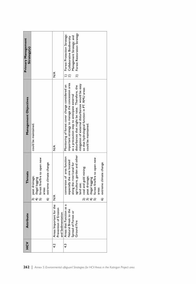
262 | Annex 5: Environmental afeguard Strategies for HCV Areas in the Katingan Project area
HC
V
Att
rib
ute
T
hre
ats
Man
agem
ent
Ob
ject
ives
P
rim
ary
Man
agem
ent
Str
ateg
y(s)
3)
peat
dra
inag
e;
4)ill
egal
logg
ing
5)fo
rest
fire
/fire
to o
pen
new
ar
eas
6)ex
trem
e cl
imat
e ch
ange
coul
d be
mai
ntai
ned.
4.2
Are
as Im
port
ant
for
the
Prev
ention
of E
rosi
on
and
Sedi
men
tation
N/A
N
/A
N/A
4.3
Are
as t
hat
Func
tion
as a
N
atur
al B
reak
to t
he
Spre
ad o
f Fo
rest
or
Gro
und
Fire
conv
ersi
on
of
area
func
tion
espe
cial
ly t
he o
ne lo
cate
d al
ong
the
riv
er/c
anal
for
agri
cultur
e, g
arde
n an
d oth
er
land
use
; 2)
coal
and
gold
min
ing;
3)
peat
dra
inag
e;
4)ill
egal
logg
ing
5)fo
rest
fire
/fire
to o
pen
new
ar
eas
6)ex
trem
e cl
imat
e ch
ange
Moni
tori
ng o
f fore
st c
ove
r ch
ange
cons
ider
ed a
n im
port
ant
stra
tegy
to m
anag
e th
e co
nces
sion
area
as
a p
reca
utio
n st
ep t
o a
ntic
ipat
e ex
tern
al
dist
urba
nces
tha
t m
ight
be
rais
e.
The
refo
re, t
he
mitig
atio
n of e
xter
nal d
istu
rban
ces
woul
d be
eas
y so
tha
t hy
dro
logi
cal f
unct
ion
in P
T. R
MU
are
as
coul
d be
mai
ntai
ned.
1)Fo
rest
Pro
tect
ion
Stra
tegy
; 2)
Colla
bora
tive
Bio
dive
rsity
Man
agem
ent
Stra
tegy
; and
3)
Fore
st R
esto
ration
Stra
tegy
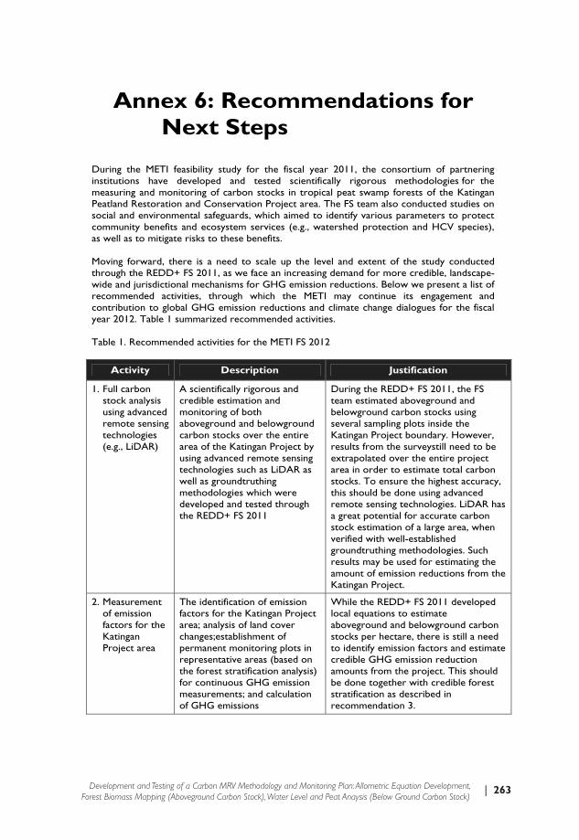
| 263Development and Testing of a Carbon MRV Methodology and Monitoring Plan: Allometric Equation Development, Forest Biomass Mapping (Aboveground Carbon Stock), Water Level and Peat Anaysis (Below Ground Carbon Stock)
Annex 6: Recommendations for Next Steps
During the METI feasibility study for the fiscal year 2011, the consortium of partnering institutions have developed and tested scientifically rigorous methodologies for the measuring and monitoring of carbon stocks in tropical peat swamp forests of the Katingan Peatland Restoration and Conservation Project area. The FS team also conducted studies on social and environmental safeguards, which aimed to identify various parameters to protect community benefits and ecosystem services (e.g., watershed protection and HCV species), as well as to mitigate risks to these benefits. Moving forward, there is a need to scale up the level and extent of the study conducted through the REDD+ FS 2011, as we face an increasing demand for more credible, landscape-wide and jurisdictional mechanisms for GHG emission reductions. Below we present a list of recommended activities, through which the METI may continue its engagement and contribution to global GHG emission reductions and climate change dialogues for the fiscal year 2012. Table 1 summarized recommended activities. Table 1. Recommended activities for the METI FS 2012
Activity Description Justification
1. Full carbon stock analysis using advanced remote sensing technologies (e.g., LiDAR)
A scientifically rigorous and credible estimation and monitoring of both aboveground and belowground carbon stocks over the entire area of the Katingan Project by using advanced remote sensing technologies such as LiDAR as well as groundtruthing methodologies which were developed and tested through the REDD+ FS 2011
During the REDD+ FS 2011, the FS team estimated aboveground and belowground carbon stocks using several sampling plots inside the Katingan Project boundary. However, results from the surveystill need to be extrapolated over the entire project area in order to estimate total carbon stocks. To ensure the highest accuracy, this should be done using advanced remote sensing technologies. LiDAR has a great potential for accurate carbon stock estimation of a large area, when verified with well-established groundtruthing methodologies. Such results may be used for estimating the amount of emission reductions from the Katingan Project.
2. Measurement of emission factors for the Katingan Project area
The identification of emission factors for the Katingan Project area; analysis of land cover changes;establishment of permanent monitoring plots in representative areas (based on the forest stratification analysis) for continuous GHG emission measurements; and calculation of GHG emissions
While the REDD+ FS 2011 developed local equations to estimate aboveground and belowground carbon stocks per hectare, there is still a need to identify emission factors and estimate credible GHG emission reduction amounts from the project. This should be done together with credible forest stratification as described in recommendation 3.
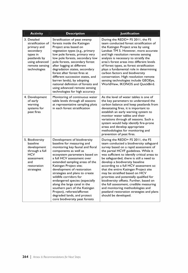
264 | Annex 6: Recommendations for Next Steps
Activity Description Justification
3. Detailed stratification of primary and secondary types in peatlands by using advanced remote sensing technologies
Stratification of peat swamp forests inside the Katingan Project area based on vegetation types (e.g., primary low pole forests, primary very low pole forests, secondary low pole forests, secondary forest after logging at different degradation states, secondary forest after forest fires at different succession states, and barren lands), by adopting national definition of forests and using advanced remote sensing technologies for high accuracy
During the REDD+ FS 2011, the FS team conducted forest stratification of the Katingan Project area by using Landsat TM 5. However, more accurate and high resolution remote sensing analysis is necessary to stratify the area’s forest areas into different levels of forest types, as forest stratification plays a fundamental role in determining carbon factors and biodiversity conservation. High resolution remote sensing technologies include GEOEye, WorldView, IKONOS and QuickBird.
4. Development of early warning systems for peat fires
Monitoring of continuous water table levels through all seasons at representative sampling plots in each forest stratification
As the level of water tables is one of the key parameters to understand the carbon balance and keep peatlands from devastating fires, it is important to establish an early warning system to monitor water tables and their variations through all seasons. Such a system would help identify fire-prone areas and develop appropriate methodologies for monitoring and prevention of peat fires.
5. Biodiversity baseline development through a full HCV assessment and restoration strategies
Development of biodiversity baseline for measuring and monitoring key faunal and floral components as well as ecosystem parameters based on a full HCV assessment over extended sampling areas of the Katingan Project site; development of restoration strategies and plans to create wildlife corridors for endangered species (especially along the large canal in the southern part of the Katingan Project), reforest/afforest degraded lands, and protect core biodiversity peat forests
During the REDD+ FS 2011, the FS team conducted a biodiversity safeguard survey based on a rapid assessment of the partial HCVF guidelines. While it was sufficient to identify critical areas to be safeguarded, there is still a need to develop a biodiversity baseline according to a full HCV assessment so that the entire Katingan Project site may be stratified based on HCV priorities and potentially qualified for biodiversity offsets. Further, based on the full assessment, credible measuring and monitoring methodologies and peatland restoration strategies and plans should be developed.
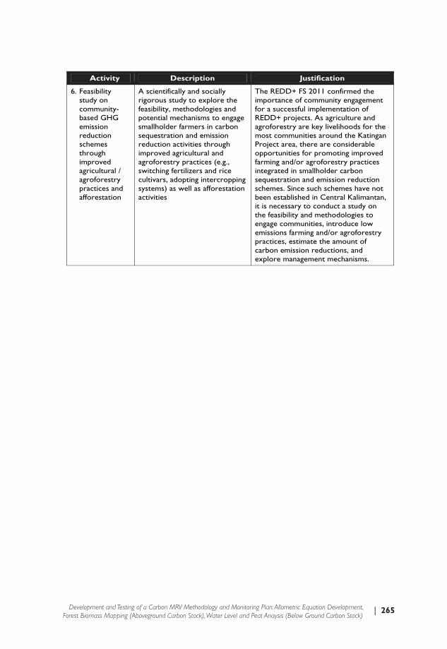
| 265Development and Testing of a Carbon MRV Methodology and Monitoring Plan: Allometric Equation Development, Forest Biomass Mapping (Aboveground Carbon Stock), Water Level and Peat Anaysis (Below Ground Carbon Stock)
Activity Description Justification
6. Feasibility study on community-based GHG emission reduction schemes through improved agricultural / agroforestry practices and afforestation
A scientifically and socially rigorous study to explore the feasibility, methodologies and potential mechanisms to engage smallholder farmers in carbon sequestration and emission reduction activities through improved agricultural and agroforestry practices (e.g., switching fertilizers and rice cultivars, adopting intercropping systems) as well as afforestation activities
The REDD+ FS 2011 confirmed the importance of community engagement for a successful implementation of REDD+ projects. As agriculture and agroforestry are key livelihoods for the most communities around the Katingan Project area, there are considerable opportunities for promoting improved farming and/or agroforestry practices integrated in smallholder carbon sequestration and emission reduction schemes. Since such schemes have not been established in Central Kalimantan, it is necessary to conduct a study on the feasibility and methodologies to engage communities, introduce low emissions farming and/or agroforestry practices, estimate the amount of carbon emission reductions, and explore management mechanisms.


ISBN: 978-602-7672-14-7
9 786027 672147
Executing AgencyCenter for Research and Development on Climate Change and Policy Forestry Research and Development Agency (FORDA)
Starting date : 1 October 2011Duration : 6 (Six) months
Host Government Republic of Indonesia
ITTO PD 73/89 (F,M,I) Phase IIFEASIBILITY STUDY ON REDD+
IN CENTRAL KALIMANTAN INDONESIA
Methodology Design Document for Reducing Emissions from Deforestation and
Degradation of Undrained Peat Swamp Forests in Central Kalimantan, Indonesia
IT OT
STARLING RESOURCES
Erica Meta SmithSteven De Gryze
Jeff Silverman Rezal Kusumaatmadja
Taryono DarusmanMartin Hardiono
I Wayan Susi DharmawanSulistyo A. Siran
Virni Budi Arifanti
Executing AgencyCenter for Research and Development on Climate Change and Policy Forestry Research and Development Agency (FORDA)
Starting date : 1 October 2011Duration : 6 (Six) months
Host Government Republic of Indonesia
ITTO PD 73/89 (F,M,I) Phase IIFEASIBILITY STUDY ON REDD+
IN CENTRAL KALIMANTAN INDONESIA
Methodology Design Document for Reducing Emissions from Deforestation and Degradation of Undrained Peat Swamp Forests
in Central Kalimantan, Indonesia
IT OT
STARLING RESOURCES
Sulistyo A. SiranRumi Naito
I Wayan Susi DharmawanSubarudi
Titiek Setyawati