Iterative Normalization: Beyond Standardization towards Efficient Whitening

Lei Huang Yi Zhou Fan Zhu Li Liu Ling Shao

Inception Institute of Artificial Intelligence (IIAI), Abu Dhabi, UAE

{lei.huang, yi.zhou, fan.zhu, li.liu, ling.shao} @inceptioniai.org

Abstract

Batch Normalization (BN) is ubiquitously employed for

accelerating neural network training and improving the gen-

eralization capability by performing standardization within

mini-batches. Decorrelated Batch Normalization (DBN) fur-

ther boosts the above effectiveness by whitening. However,

DBN relies heavily on either a large batch size, or eigen-

decomposition that suffers from poor efficiency on GPUs. We

propose Iterative Normalization (IterNorm), which employs

Newton’s iterations for much more efficient whitening, while

simultaneously avoiding the eigen-decomposition. Further-

more, we develop a comprehensive study to show IterNorm

has better trade-off between optimization and generalization,

with theoretical and experimental support. To this end, we

exclusively introduce Stochastic Normalization Disturbance

(SND), which measures the inherent stochastic uncertainty

of samples when applied to normalization operations. With

the support of SND, we provide natural explanations to sev-

eral phenomena from the perspective of optimization, e.g.,

why group-wise whitening of DBN generally outperforms

full-whitening and why the accuracy of BN degenerates with

reduced batch sizes. We demonstrate the consistently im-

proved performance of IterNorm with extensive experiments

on CIFAR-10 and ImageNet over BN and DBN.

1. Introduction

Centering, scaling and decorrelating the input data is

known as data whitening, which has demonstrated enormous

success in speeding up training [25]. Batch Normalization

(BN) [19] extends the operations from the input layer to

centering and scaling activations of each intermediate layer

within a mini-batch so that each neuron has a zero mean and

a unit variance (Figure 1 (a)). BN has been extensively used

in various network architectures [11, 43, 12, 50, 42, 14] for

its benefits in improving both the optimization efficiency

[19, 9, 21, 5, 37] and generalization capability [19, 3, 5, 48].

However, instead of performing whitening, BN is only capa-

ble of performing standardization, which centers and scales

the activations but does not decorrelate them [19]. On the

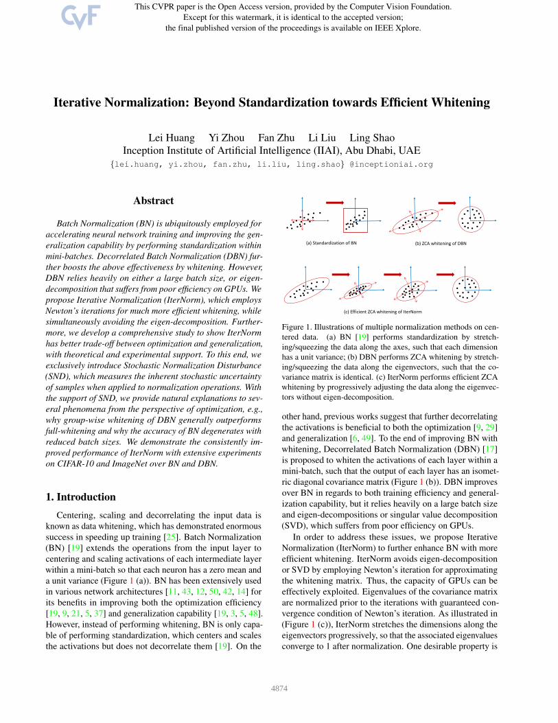
(a) Standardization of BN (b) ZCA whitening of DBN

(c) Efficient ZCA whitening of IterNorm

Figure 1. Illustrations of multiple normalization methods on cen-

tered data. (a) BN [19] performs standardization by stretch-

ing/squeezing the data along the axes, such that each dimension

has a unit variance; (b) DBN performs ZCA whitening by stretch-

ing/squeezing the data along the eigenvectors, such that the co-

variance matrix is identical. (c) IterNorm performs efficient ZCA

whitening by progressively adjusting the data along the eigenvec-

tors without eigen-decomposition.

other hand, previous works suggest that further decorrelating

the activations is beneficial to both the optimization [9, 29]

and generalization [6, 49]. To the end of improving BN with

whitening, Decorrelated Batch Normalization (DBN) [17]

is proposed to whiten the activations of each layer within a

mini-batch, such that the output of each layer has an isomet-

ric diagonal covariance matrix (Figure 1 (b)). DBN improves

over BN in regards to both training efficiency and general-

ization capability, but it relies heavily on a large batch size

and eigen-decompositions or singular value decomposition

(SVD), which suffers from poor efficiency on GPUs.

In order to address these issues, we propose Iterative

Normalization (IterNorm) to further enhance BN with more

efficient whitening. IterNorm avoids eigen-decomposition

or SVD by employing Newton’s iteration for approximating

the whitening matrix. Thus, the capacity of GPUs can be

effectively exploited. Eigenvalues of the covariance matrix

are normalized prior to the iterations with guaranteed con-

vergence condition of Newton’s iteration. As illustrated in

(Figure 1 (c)), IterNorm stretches the dimensions along the

eigenvectors progressively, so that the associated eigenvalues

converge to 1 after normalization. One desirable property is

4874

that the convergence speed of IterNorm along the eigenvec-

tors is proportional to the associated eigenvalues [4]. This

means the dimensions that correspond to small/zero (when

a small batch size is applied) eigenvalues can be largely

ignored, given a fixed number of iterations. As a conse-

quence, the sensitivity of IterNorm against batch size can be

significantly reduced.

When the data batch is undersized, it is known that the

performance of both whitening and standardization on the

test data can be significantly degraded [18, 48]. However,

beyond our expectation, we observe that the performance

on the training set also significantly degenerates under the

same condition. We further observe such a phenomenon

is caused by the stochasticity introduced by the mini-batch

based normalization [44, 39]. To allow a more comprehen-

sive understanding and evaluation about the stochasticity,

we introduce Stochastic Normalization Disturbance (SND),

which is discussed in Section 4. With the support of SND,

we provide a thorough analysis regarding the performance

of normalization methods, with respect to the batch size and

feature dimensions, and show that IterNorm has better trade-

off between optimization and generalization. Experiments

on CIFAR-10 [22] and ILSVRC-2012 [8] demonstrate the

consistent improvements of IterNorm over BN and DBN.

2. Related Work

Normalized activations [38, 33, 31, 46] have long been

known to benefit neural networks training. Some research

methodologies attempt to normalize activations by viewing

the population statistics as parameters and estimating them

directly during training [31, 46, 9]. Some of these meth-

ods include activations centering in Restricted Boltzmann

Machine [31]/feed-forward neural networks [46] and acti-

vations whitening [9, 29]. This type of normalization may

suffer from instability (such as divergence or gradient explo-

sion) due to 1) inaccurate approximation to the population

statistics with local data samples [46, 19, 18, 17] and 2) the

internal-covariant shift problem [19].

Ioffe et al., [19] propose to perform normalization as a

function over mini-batch data and back-propagate through

the transformation. Multiple standardization options have

been discovered for normalizing mini-batch data, including

the L2 standardization [19], the L1-standardization [47, 13]

and the L∞-standardization [13]. One critical issue with

these methods, however, is that it normally requires a reason-

able batch size for estimating the mean and variance. In order

to address such an issue, a significant number of standardiza-

tion approaches are proposed [3, 48, 34, 30, 18, 27, 45, 24, 7].

Our work develops in an orthogonal direction to these ap-

proaches, and aims at improving BN with decorrelated acti-

vations.

Beyond standardization, Huang et al. [17] propose DBN,

which uses ZCA-whitening by eigen-decomposition and

back-propagates the transformation. Our approach aims at a

much more efficient approximation of the ZCA-whitening

matrix in DBN, and suggests that approximating whitening

is more effective based on the analysis shown in Section 4.

Our approach is also related to works that normalize the

network weights (e.g., either through re-parameterization

[36, 16, 15] or weight regularization [23, 32, 35]), and that

specially design either scaling coefficients & bias values

[1] or nonlinear function [20], to normalize activation im-

plicitly [39]. IterNorm differs from these work in that it is

a data dependent normalization, while these normalization

approaches are independent of the data.

Newton’s iteration is also employed in several other deep

neural networks. These methods focus on constructing bi-

linear [28] or second-order pooling [26] by constraining the

power of the covariance matrix and are limited to produc-

ing fully-connected activations, while our work provides

a generic module that can be ubiquitously built in various

neural network frameworks. Besides, our method computes

the square root inverse of the covariance matrix, instead of

calculating the square root of the covariance matrix [28, 26].

3. Iterative Normalization

Let X ∈ Rd×m be a data matrix denoting the mini-

batch input of size m in certain layer. BN [19] works by

standardizing the activations over the mini-batch input:

�X = φStd(X) = Λ−

1

2

std(X− µ · 1T ), (1)

where µ = 1mX · 1 is the mean of X, Λstd =

diag(σ21 , . . . ,σ

2d) + �I, σ2

iis the dimension-wise variance

corresponding to the i-th dimension, 1 is a column vector of

all ones, and � > 0 is a small number to prevent numerical

instability. Intuitively, standardization ensures that the nor-

malized output gives equal importance to each dimension by

multiplying the scaling matrix Λ−

1

2

std(Figure 1 (a)).

DBN [17] further uses ZCA whitening to produce thewhitened output as1:

φZCA(X) = DΛ−

1

2DT (X− µ · 1T ), (2)

where Λ = diag(σ1, . . . ,σd) and D = [d1, ...,dd] are

the eigenvalues and associated eigenvectors of Σ, i.e. Σ =DΛD

T . Σ = 1m(X − µ · 1T )(X − µ · 1T )T + �I is the

covariance matrix of the centered input. ZCA whitening

works by stretching or squeezing the dimensions along the

eigenvectors such that the associated eigenvalues to be 1(Figure 1 (b)). Whitening the activation ensures that all di-

mensions along the eigenvectors have equal importance in

the subsequent linear layer.

One crucial problem of ZCA whitening is that calculat-

ing the whitening matrix requires eigen-decomposition or

1DBN and BN both use learnable dimension-wise scale and shift param-

eters to recover the possible loss of representation capability.

4875

Algorithm 1 Whitening activations with Newton’s iteration.

1: Input: mini-batch inputs X ∈ Rd×m.

2: Hyperparameters: �, iteration number T .

3: Output: the ZCA-whitened activations �X.

4: calculate mini-batch mean: µ = 1

mX · 1.

5: calculate centered activation: XC = X− µ · 1T .

6: calculate covariance matrix: Σ = 1

mXCX

TC + �I.

7: calculate trace-normalized covariance matrix ΣN by Eqn .4.

8: P0 = I.

9: for k = 1 to T do

10: Pk = 1

2(3Pk−1 −P

3

k−1ΣN )11: end for

12: calculate whitening matrix: Σ−

1

2 = PT /�

tr(Σ).

13: calculate whitened output: �X = Σ−

1

2XC .

SVD, as shown in Eqn. 2, which heavily constrains its prac-

tical applications. We observe that Eqn. 2 can be viewed

as the square root inverse of the covariance matrix denoted

by Σ−

1

2 , which multiplies the centered input. The square

root inverse of one specific matrix can be calculated us-

ing Newton’s iteration methods [4], which avoids executing

eigen-decomposition or SVD.

3.1. Computing Σ−

1

2 by Newton’s Iteration

Given the square matrix A, Newton’s method calculates

A−

1

2 by the following iterations [4]:

�P0 = I

Pk = 1

2(3Pk−1 −P

3

k−1A), k = 1, 2, ..., T,(3)

where T is the iteration number. Pk will be converged to

A−

1

2 under the condition �A− I�2 < 1.In terms of applying Newton’s methods to calculate the in-

verse square root of the covariance matrix Σ−

1

2 , one crucialproblem is Σ cannot be guaranteed to satisfy the convergencecondition �Σ − I�2 < 1. That is because Σ is calculatedover mini-batch samples and thus varies during training.If the convergence condition cannot be perfectly satisfied,the training can be highly instable [4, 26]. To address thisissue, we observe that one sufficient condition for conver-gence is to ensure the eigenvalues of the covariance matrixare less than 1. We thus propose to construct a transforma-tion ΣN = F (Σ) such that �ΣN�2 < 1, and ensure thetransformation is differentiable such that the gradients canback-propagate through this transformation. One feasibletransformation is to normalize the eigenvalue as follows:

ΣN = Σ/tr(Σ), (4)

where tr(Σ) indicates the trace of Σ. Note that ΣN is alsoa semi-definite matrix and thus all of its eigenvalues aregreater than or equal to 0. Besides, ΣN has the property thatthe sum of its eigenvalues is 1. Therefore, ΣN can surelysatisfy the convergence condition. We can thus calculate

the inverse square root Σ−

1

2

Nby Newton’s method as Eqn.

3. Given Σ−

1

2

N, we can compute Σ

−

1

2 based on Eqn. 4, asfollows:

Σ−

1

2 = Σ−

1

2

N /�

tr(Σ). (5)

Given Σ−

1

2 , it’s easy to whiten the activations by multiplying

Σ−

1

2 with the centered inputs. In summary, Algorithm 1

describes our proposed methods for whitening the activations

in neural networks.

Our method first normalizes the eigenvalues of the covari-

ance matrix, such that the convergence condition of New-

ton’s iteration is satisfied. We then progressively stretch the

dimensions along the eigenvectors, such that the final asso-

ciate eigenvalues are all “1”, as shown in Figure 1 (c). Note

that the speed of convergence of the eigenvectors is propor-

tional to the associated eigenvalues [4]. That is, the larger

the eigenvalue is, the faster its associated dimension along

the eigenvectors converges. Such a mechanism is a remark-

able property to control the extent of whitening, which is

essential for the success of whitening activations, as pointed

out in [17], and will be further discussed in Section 4.

3.2. Back-propagation

As pointed out by [19, 17], viewing standardization orwhitening as functions over the mini-batch data and back-propagating through the normalized transformation are es-sential for stabilizing training. Here, we derive the back-propagation pass of IterNorm. Denoting L as the loss func-tion, the key is to calculate ∂L

∂Σ, given ∂L

∂Σ−1/2 . Let’s denote

PT = Σ−

1

2

N, where T is the iteration number. Based on the

chain rules, we have:

∂L

∂PT=

1�tr(Σ)

∂L

∂Σ−

1

2

∂L

∂ΣN= −

1

2

T�

k=1

(P3

k−1)T ∂L

∂Pk

∂L

∂Σ=

1

tr(Σ)

∂L

∂ΣN−

1

(tr(Σ))2tr(

∂L

∂ΣN

T

Σ)I

−1

2(tr(Σ))3/2tr((

∂L

∂Σ−1/2)TPT )I, (6)

where ∂L∂Pk

can be calculated by following iterations:

∂L

∂Pk−1

=3

2

∂L

∂Pk−

1

2

∂L

∂Pk(P2

k−1ΣN )T −1

2(P2

k−1)T ∂L

∂PkΣ

TN

−1

2(Pk−1)

T ∂L

∂Pk(Pk−1ΣN )T , k = T, ..., 1. (7)

Note that in Eqn. 4 and 5, tr(Σ) is a function for mini-

batch examples and is needed to back-propagate through it

to stabilize the training. Algorithm 2 summarizes the back-

propagation pass of our proposed IterNorm. More details of

back-propagation derivations are shown in supplementary

materials.

4876

Algorithm 2 The respective backward pass of Algorithm 1.

1: Input: mini-batch gradients respect to whitened activations:∂L

∂ �X. auxiliary data from respective forward pass: (1) XC ; (2)

Σ−

1

2 ; (3) {Pk}.

2: Output: the gradients with respect to the inputs: ∂L∂X

.

3: calculate the gradients with respect to Σ−

1

2 : ∂L

∂Σ−

1

2

= ∂L

∂ �XX

TC .

4: calculate ∂L∂Σ

based on Eqn. 6 and 7.

5: calculate: f = 1

m∂L

∂ �X· 1.

6: calculate: ∂L∂X

= Σ−

1

2 ( ∂L

∂ �X− f · 1T ) + 1

m( ∂L∂Σ

+ ∂L∂Σ

T)XC .

3.3. Training and Inference

Like the previous normalizing activation methods [19, 3,17, 48], our IterNorm can be used as a module and insertedinto a network extensively. Since IterNorm is also a methodfor mini-batch data, we use the running average to calculate

the population mean µ and whitening matrix �Σ−

1

2 , whichis used during inference. Specifically, during training, we

initialize µ as 0 and �Σ−

1

2 as I and update them as follows:

µ = (1− λ) µ+ λ µ

�Σ−

1

2 = (1− λ)�Σ−

1

2 + λΣ−

1

2 , (8)

where µ and Σ−

1

2 are the mean and whitening matrix cal-

culated within each mini-batch during training, and λ is the

momentum of running average.

Additionally, we also use the extra learnable parameters

γ and β, as in previous normalization methods [19, 3, 17,

48], since normalizing the activations constrains the model’s

capacity for representation. Such a process has been shown

to be effective [19, 3, 17, 48].

Convolutional Layer For a CNN, the input is XC ∈R

h×w×d×m, where h and w indicate the height and width

of the feature maps, and d and m are the number of feature

maps and examples, respectively. Following [19], we view

each spatial position of the feature map as a sample. We thus

unroll XC as X ∈ Rd×(mhw) with m×h×w examples and

d feature maps. The whitening operation is performed over

the unrolled X.

Computational Cost The main computation of our Iter-

Norm includes calculating the covariance matrix, the itera-

tion operation and the whitened output. The computational

costs of the first and the third operation are equivalent to the

1 × 1 convolution. The second operation’s computational

cost is Td3. Our method is comparable to the convolu-

tion operation. To be specific, given the internal activation

XC ∈ Rh×w×d×m, the 3 × 3 convolution with the same

input and output feature maps costs 9hwmd2, while our Iter-

Norm costs 2hwmd2 + Td3. The relative cost of IterNorm

for 3 × 3 convolution is 2/9 + Td/mhw. Further, we can

use group-wise whitening, as introduced in [17] to improve

the efficiency when the dimension d is large. We also com-

pare the wall-clock time of IterNorm, DBN [17] and 3× 3convolution in supplementary materials.

During inference, IterNorm can be viewed as a 1 × 1convolution and merged to adjacent convolutions. Therefore,

IterNorm does not introduce any extra costs in memory or

computation during inference.

4. Stochasticity of Normalization

Mini-batch based normalization methods are sensitive to

the batch size [18, 17, 48]. As described in [17], fully whiten-

ing the activation may suffer from degenerate performance

while the number of data in a mini-batch is not sufficient.

They [17] thus propose to use group-wise whitening [17].

Furthermore, standardization also suffers from degenerated

performance under the scenario of micro-batch [45]. These

works argue that undersized data batch makes the estimated

population statistics highly noisy, which results in a degener-

ating performance during inference [3, 18, 48].

In this section, we will provide a more thorough analysis

regarding the performance of normalization methods, with

respect to the batch size and feature dimensions. We show

that normalization (standardization or whitening) with un-

dersized data batch not only suffers from degenerate perfor-

mance during inference, but also encounter the difficulty in

optimization during training. This is caused by the Stochastic

Normalization Disturbance (SND), which we will describe.

4.1. Stochastic Normalization Disturbance

Given a sample x ∈ Rd from a distribution Pχ, we take

a sample set XB = {x1, ...,xB ,xi ∼ Pχ} with a size ofB. We denote the normalization operation as F (·) and thenormalized output as x = F (XB ;x). For a certain x, XB

can be viewed as a random variable [2, 44]. x is thus arandom variable which shows the stochasticity. It’s interest-ing to explore the statistical momentum of x to measure themagnitude of the stochasticity. Here we define the StochasticNormalization Disturbance (SND) for the sample x over thenormalization F (·) as:

∆F (x) = EXB(�x−EXB (x)�2). (9)

It’s difficult to accurately compute this momentum if nofurther assumptions are made over the random variable X

B ,however, we can explore its empirical estimation over thesampled sets as follows:

�∆F (x) =1

s

s�

i=1

�F (XBi ;x)−

1

s

s�

j=1

F (XBj ;x)�, (10)

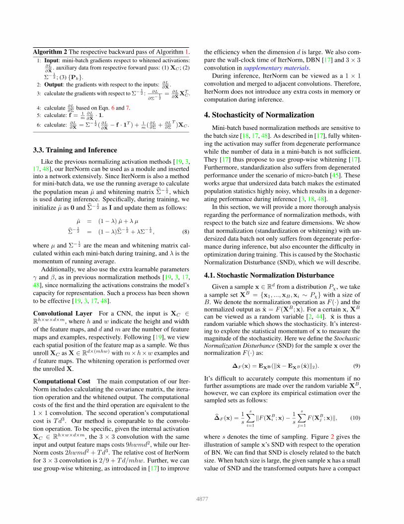
where s denotes the time of sampling. Figure 2 gives the

illustration of sample x’s SND with respect to the operation

of BN. We can find that SND is closely related to the batch

size. When batch size is large, the given sample x has a small

value of SND and the transformed outputs have a compact

4877

-3 -2 -1 0 1 2 3-3

-2

-1

0

1

2

3

Examples

Normalized Points

Sampled Point

"(x)=0.0016

(a) batch size of 16

-3 -2 -1 0 1 2 3-3

-2

-1

0

1

2

3

Examples

Normalized Points

Sampled Point

"(x)=0.0007

(b) batch size of 64

Figure 2. Illustration of SND with different batch sizes. We sample

3000 examples (black points) from Gaussian distribution. We show

a given example x (red cross) and its BN outputs (blue plus sign),

when normalized over different sample sets XB . (a) and (b) show

the results with batch sizes B of 16 and 64, respectively.

distribution. As a consequence, the stochastic uncertainty x

can be low.

SND can be used to evaluate the stochasticity of a sam-

ple after the normalization operation, which works like the

dropout rate [41]. We can further define the normalization

operation F (·)’s SND as: ∆F = Ex(∆(x)) and it’s em-

pirical estimation as �∆F = 1N

�N

i=1�∆(x) where N is the

number of sampled examples. ∆F describes the magnitudes

of stochasticity for corresponding normalization operations.

Exploring the exact statistic behavior of SND is difficult

and out of the scope of this paper. We can, however, explore

the relationship of SND related to the batch size and feature

dimension. We find that our defined SND gives a reasonable

explanation to why we should control the extent of whitening

and why mini-batch based normalizations have a degenerate

performance when given a small batch size.

4.2. Controlling the Extent of Whitening

We start with experiments on multi-layer perceptron

(MLP) over MNIST dataset, by using the full batch gra-

dient (batch size =60,000), as shown in Figure 3 (a). We find

that all normalization methods significantly improve the per-

formance. One interesting observation is that full-whitening

the activations with such a large batch size still underper-

forms the approximate-whitening of IterNorm, in terms of

training efficiency. Intuitively, full-whitening the activations

may lead to amplifying the dimension with small eigenval-

ues, which may correspond to the noise. Exaggerating this

noise may be harmful to learning, especially lowering down

the generalization capability as shown in Figure 3 (a) that

DBN has diminished test performance. We provide further

analysis based on SND, along with the conditioning analysis.

It has been shown that improved conditioning can accelerate

training [25, 9], while increased stochasticity can slow down

training but likely to improve generalization [41] .

We experimentally explore the consequent effects of im-

proved conditioning [25] with SND through BN (standard-

ization), DBN (full-whitening) and IterNorm (approximate-

0 20 40 60 80 100

Iterations

0

50

100

Err

or

plain

BN

DBN

IterNorm

(a) batch size of 60,000

0 1000 2000 3000 4000 5000

Iterations (x100)

0

0.5

1

1.5

2

2.5

Tra

inin

g loss

plain

BN

IterNorm

(b) batch size of 2

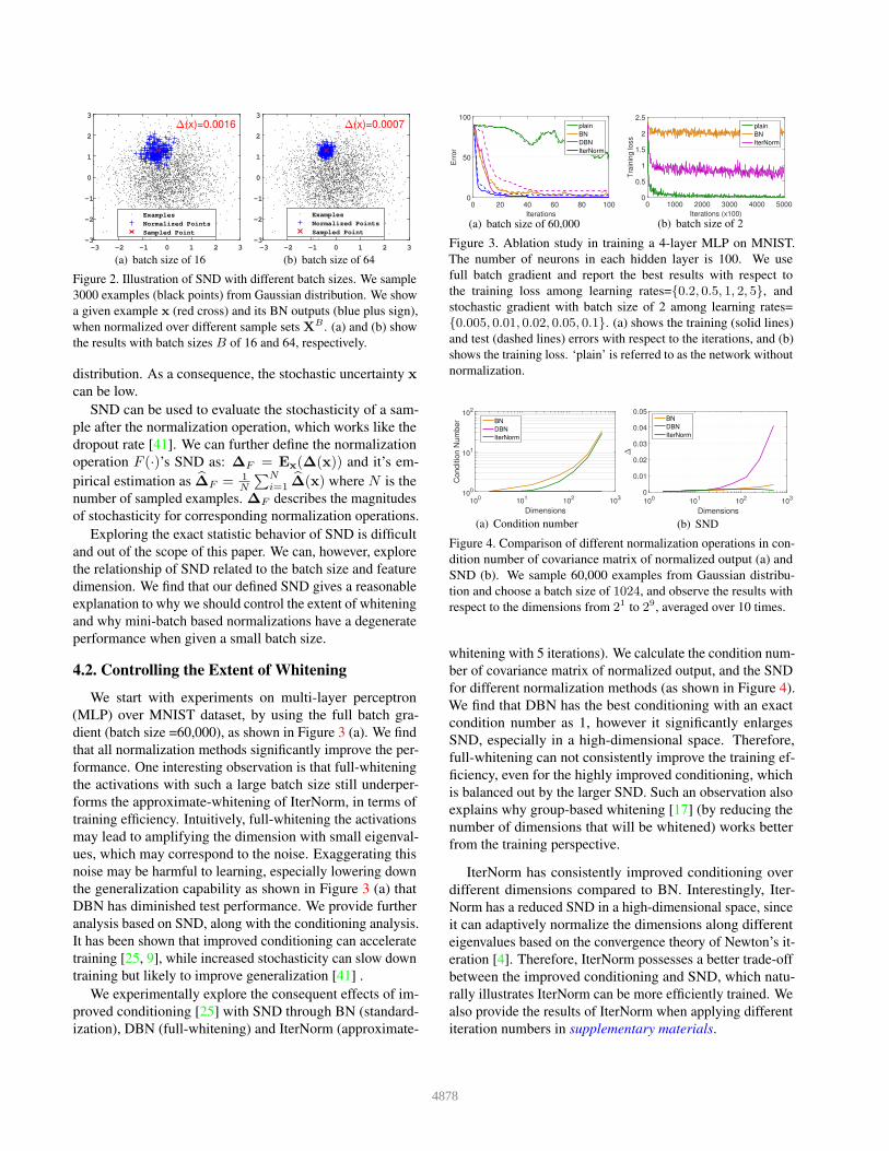
Figure 3. Ablation study in training a 4-layer MLP on MNIST.

The number of neurons in each hidden layer is 100. We use

full batch gradient and report the best results with respect to

the training loss among learning rates={0.2, 0.5, 1, 2, 5}, and

stochastic gradient with batch size of 2 among learning rates=

{0.005, 0.01, 0.02, 0.05, 0.1}. (a) shows the training (solid lines)

and test (dashed lines) errors with respect to the iterations, and (b)

shows the training loss. ‘plain’ is referred to as the network without

normalization.

100

101

102

103

Dimensions

100

101

102

Conditio

n N

um

ber BN

DBN

IterNorm

(a) Condition number

100

101

102

103

Dimensions

0

0.01

0.02

0.03

0.04

0.05

"

BN

DBN

IterNorm

(b) SND

Figure 4. Comparison of different normalization operations in con-

dition number of covariance matrix of normalized output (a) and

SND (b). We sample 60,000 examples from Gaussian distribu-

tion and choose a batch size of 1024, and observe the results with

respect to the dimensions from 21 to 29, averaged over 10 times.

whitening with 5 iterations). We calculate the condition num-

ber of covariance matrix of normalized output, and the SND

for different normalization methods (as shown in Figure 4).

We find that DBN has the best conditioning with an exact

condition number as 1, however it significantly enlarges

SND, especially in a high-dimensional space. Therefore,

full-whitening can not consistently improve the training ef-

ficiency, even for the highly improved conditioning, which

is balanced out by the larger SND. Such an observation also

explains why group-based whitening [17] (by reducing the

number of dimensions that will be whitened) works better

from the training perspective.

IterNorm has consistently improved conditioning over

different dimensions compared to BN. Interestingly, Iter-

Norm has a reduced SND in a high-dimensional space, since

it can adaptively normalize the dimensions along different

eigenvalues based on the convergence theory of Newton’s it-

eration [4]. Therefore, IterNorm possesses a better trade-off

between the improved conditioning and SND, which natu-

rally illustrates IterNorm can be more efficiently trained. We

also provide the results of IterNorm when applying different

iteration numbers in supplementary materials.

4878

0 200 400 600 800 1000

Batch Size

0

0.01

0.02

0.03

0.04

"

BN

IterNorm

(a)

100

101

102

103

Dimensions

0

0.02

0.04

0.06

0.08

"

BN

IterNorm

(b)

Figure 5. Illustration of the micro-batch problem of BN from the

perspective of SND. (a) shows the SND with respect to batch sizes

under the dimension of 128. (b) shows the SND with respect to

dimensions under the batch size of 2.

4.3. Micro-batch Problem of BN

BN suffers from degenerate test performance if the batch

data is undersized [48]. We also show that BN suffers from

the optimization difficulty with a small batch size. We show

the experimental results on MNIST dataset with a batch

size of 2 in Figure 3 (b). We find that BN can hardly learn

and produces random results, while the naive network with-

out normalization learns well. Such an observation clearly

shows that BN suffers from more difficulties in training with

undersized data batch.

For an in-depth investigation, we sample the data from

the dimension of 128 (Figure 5 (a)), and find that BN has a

significantly increased SND. With increasing batch sizes, the

SND of BN can be gradually reduced. Meanwhile, reduced

SND leads to more stable training. When we fix the batch

size to 2 and vary the dimension, (as shown in Figure 5 (b)),

we observe that the SND of BN can be reduced with a low

dimension. On the contrary, the SND of BN can be increased

in a high-dimensional space. Thus, it can be explained why

BN suffers from the difficulty during with a small batch, and

why group-based normalization [48] (by reducing the dimen-

sion and adding the examples to be standardized implicitly)

alleviates the problem.

Compared to BN, IterNorm is much less sensitive to a

small batch size in producing SND. Besides, the SND of

IterNorm is more stable, even with a significantly increased

dimension. Such characteristics of IterNorm are mainly at-

tributed to its adaptive mechanism in normalization, that it

stretches the dimensions along large eigenvalues and corre-

spondingly ignores small eigenvalues, given a fixed number

of iterations [4].

5. Experiments

We evaluate IterNorm with CNNs on CIFAR datasets

[22] to show that the better optimization efficiency

and generalization capability, compared to BN [19] and

DBN [17]. Furthermore, IterNorm with residual net-

works will be applied to show the performance improve-

ment on CIFAR-10 and ImageNet [8] classification tasks.

The code to reproduce the experiments is available at

https://github.com/huangleiBuaa/IterNorm.

5.1. Sensitivity Analysis

We analyze the proposed methods on CNN architectures

over the CIFAR-10 dataset [22], which contains 10 classes

with 50k training examples and 10k test examples. The

dataset contains 32× 32 color images with 3 channels. We

use the VGG networks [40] tailored for 32× 32 inputs (16

convolution layers and 1 fully-connected layers), and the de-

tails of the networks are shown in supplementary materials.

The datasets are preprocessed with a mean-subtraction

and variance-division. We also execute normal data augmen-

tation operation, such as a random flip and random crop with

padding, as described in [11].

Experimental Setup We use SGD with a batch size of

256 to optimize the model. We set the initial learning rate

to 0.1, then divide the learning rate by 5 at 60 and 120

epochs, and finish the training at 160 epochs. All results are

averaged over 3 runs. For DBN, we use a group size of 16

as recommend in [17], and we find that DBN is unstable for

a group size of 32 or above, due to the fact that the eigen-

decomposition operation cannot converge. The main reason

is that the batch size is not sufficient for DBN to full-whiten

the activation for each layer. For IterNorm, we don’t use

group-wise whitening in the experiments, unless otherwise

stated.

Effect of Iteration Number The iteration number T of

our IterNorm controls the extent of whitening. Here we

explore the effects of T on performance of IterNorm, for a

range of {0, 1, 3, 5, 7}. Note that when T = 0, our method is

reduced to normalizing the eigenvalues such that the sum of

the eigenvalues is 1. Figure 7 (a) shows the results. We find

that the smallest (T = 0) and the largest (T = 7) iteration

number both have the worse performance in terms of training

efficiency. Further, when T = 7, IterNorm has significantly

worse test performance. These observations show that (1)

whitening within an mini-batch can improve the optimiza-

tion efficiency, since IterNorm progressively stretches out the

data along the dimensions of the eigenvectors such that the

corresponding eigenvalue towards 1, with increasing itera-

tion T ; (2) controlling the extent of whitening is essential for

its success, since stretching out the dimensions along small

eigenvalue may produce large SND as described in Section

4, which not only makes estimating the population statistics

difficult — therefore causing higher test error — but also

makes optimization difficult. Unless otherwise stated, we

use an iteration number of 5 in subsequent experiments.

Effects of Group Size We also investigate the effects of

group size. We vary the group size in {256, 64, 32, 1}, com-

pared to the full-whitening operation of IterNorm (group size

of 512). Note that our IterNorm with group size of 1, like

DBN, is also reduced to Batch Normalization [19], which is

ensured by Eqn. 4 and 5. The results are shown in Figure 7

4879

0 50 100 150

Epochs

0

5

10

15

20

Err

or

BN

DBN

IterNorm

(a) basic configuration

0 50 100 150

Epochs

0

5

10

15

20

Err

or

BN

DBN

IterNorm

(b) batch size of 1024

0 50 100 150

Epochs

0

5

10

15

20

Err

or

BN

DBN

IterNorm

(c) batch size of 16

0 50 100 150

Epochs

0

5

10

15

20

Err

or

BN

DBN

IterNorm

(d) 10x larger learning rate

Figure 6. Comparison among BN, DBN and IterNorm on VGG over CIFAR-10 datasets. We report the training (solid lines) and test (dashed

lines) error with respect to epochs.

Epochs

0 50 100 150

Err

or

0

5

10

15

20Iter0Iter1Iter3Iter5Iter7

(a)Epochs

0 50 100 150

Err

or

0

5

10

15

20G512G256G64G32G1

(b)

Figure 7. Ablation studies on VGG over CIFAR-10 datasets. We

report the training (solid lines) and test (dashed lines) error curves.

(a) shows the effects of different iteration number for IterNorm; (b)

show the effects of different group size of IterNorm.

(b). We can find that our IterNorm, unlike DBN, is not sensi-

tive to the large group size, not only in training, but also in

testing. The main reason is that IterNorm gradually stretches

out the data along the dimensions of eigenvectors such that

the corresponding eigenvalue towards 1, in which the speed

of convergence for each dimension is proportional to the as-

sociated eigenvalues [4]. Even though there are many small

eigenvalue or zero in high-dimension space, IterNorm only

stretches the dimension along the associate eigenvector a

little, given small iteration T , which introduces few SND. In

practice, we can use a smaller group size, which can reduce

the computational costs. We recommend using a group size

of 64, which is proposed in the experiments of Section 5.2

and 5.3 for IterNorm.

Comparison of Baselines We compare our IterNorm with

T = 5 to BN and DBN. Under the basic configuration,

we also experiment with other configurations, including (1)

using a large batch size of 1024; (2) using a small batch

size of 16; and (3) increasing the learning rate by 10 times

and considering mini-batch based normalization is highly

dependent on the batch size and their benefits comes from

improved conditioning and therefore larger learning rate.

All experimental setups are the same, except that we search

a different learning rate in {0.4, 0.1, 0.0125} for different

batch sizes, based on the linear scaling rule [10]. Figure 6

shows the results.

We find that our proposed IterNorm converges the fastest

with respect to the epochs, and generalizes the best, com-

pared to BN and DBN. DBN also has better optimization and

0 50 100 150 200

Epochs

0

5

10

15

Err

or

BN

IterNorm

(a) WRN-28-10

0 50 100 150 200

Epochs

0

5

10

15

Err

or

BN

IterNorm

(b) WRN-40-10

Figure 8. Comparison on Wide Residual Networks over CIFAR-10

datasets. The solid line indicates the training errors and the dashed

line indicates the test errors. (a) shows the results on WRN-28-10

and (b) on WRN-40-10.

generalization capability than BN. Particularly, IterNorm re-

duces the absolute test error of BN by 0.79%, 0.53%, 1.11%,

0.75% for the four experiments above respectively, and DBN

by 0.22, 0.37, 1.05, 0.58. The results demonstrate that our

IterNorm outperforms BN and DBN in terms of optimization

quality and generalization capability.

5.2. Results on CIFAR-10 with Wide Residual Net-works

We apply our IterNorm to Wide Residual Network (WRN)

[50] to improve the performance on CIFAR-10. Following

the conventional description in [50], we use the abbrevia-

tion WRN-d-k to indicate a WRN with depth d and width

k. We adopt the publicly available Torch implementation2

and follow the same setup as in [50]. We apply IterNorm

to WRN-28-10 and WRN-40-10 by replacing all the BN

modules with our IterNorm. Figure 8 gives the training

and testing errors with respect to the training epochs. We

clearly find that the wide residual network with our proposed

IterNorm improves the original one with BN, in terms of

optimization efficiency and generalization capability. Table

1 shows the final test errors, compared to previously reported

results for the baselines and DBN [17].

The results show IterNorm improves the original WRN

with BN and DBN on CIFAR-10. In particular, our methods

reduce the test error to 3.56% on WRN-28-10, a relatively

improvement of 8.5% in performance over ‘Baseline’.

2https://github.com/szagoruyko/wide-residual-networks

4880

Method WRN-28-10 WRN-40-10

Baseline* [50] 3.89 3.80

DBN [17] 3.79 ± 0.09 3.74 ± 0.11

Baseline 3.89 ± 0.13 3.82 ± 0.11

IterNorm 3.56 ± 0.12 3.59 ± 0.07

Table 1. Test errors (%) on wide residual networks over CIFAR-10.

All results are computed over 5 random seeds, and shown in the

format of ‘mean ±std’. We replicate the ‘Baseline’ results based

on the released code in [50], which computes the median of 5 runs

on WRN-28-10 and only performs one run onWRN-40-10.

Method Top-1 Top-5

Baseline* [11] 30.43 10.76

DBN-L1* [17] 29.87 10.36

Baseline 29.76 10.39

DBN-L1 29.50 10.26

IterNorm-L1 29.34 10.22

IterNorm-Full 29.30 10.21

IterNorm-L1 + DF 28.86 10.08

Table 2. Comparison of validation errors (%, single model and

single-crop) on 18-layer residual networks on ILSVRC-2012.

‘Baseline*’ and ‘DBN-L1*’ indicate that the results are reported in

[17] with training of 90 epochs.

5.3. Results on ImageNet with Residual Network

We validate the effectiveness of our methods on residual

networks for ImageNet classification with 1000 classes [8].

We use the given official 1.28M training images as a training

set, and evaluate the top-1 and top-5 classification errors on

the validation set with 50k images.

Ablation Study on Res-18 We first execute an ablation

study on the 18-layer residual network (Res-18) to explore

multiple positions for replacing BN with IterNorm. The

models used are as follows: (a) ‘IterNorm-L1’: we only

replace the first BN module of ResNet-18, so that the decor-

related information from previous layers can pass directly

to the later layers with the identity connections described

in [17]; (b) We also replace all BN modules indicated as

‘IterNorm-full’; We follow the same experimental setup as

described in [11], except that we use 1 GPU and train over

100 epochs. We apply SGD with a mini-batch size of 256,

momentum of 0.9 and weight decay of 0.0001. The initial

learning rate is set to 0.1 and divided by 10 at 30, 60 and 90

epochs, and end the training at 100 epochs.

We find that only replacing the first BN effectively im-

proves the performance of the original residual network,

either by using DBN or IterNorm. Our IterNorm has

marginally better performance than DBN. We find that re-

placing all the layers of IterNorm has no significant im-

provement over only replacing the first layer. We conjecture

that the reason might be that the learned residual functions

Res-50 Res-101

Method Top-1 Top-5 Top-1 Top-5

Baseline* [11] 24.70 7.80 23.60 7.10

Baseline 23.95 7.02 22.45 6.29

IterNorm-L1 23.28 6.72 21.95 5.99

IterNorm-L1 + DF 22.91 6.47 21.77 5.94

Table 3. Comparison of test errors (%, single model and

single-crop) on 50/101-layer residual networks on ILSVRC-2012.

‘Baseline*’ indicates that the results are obtained from the website:

https://github.com/KaimingHe/deep-residual-networks.

tend to have small response as shown in [11], and stretching

this small response to the magnitude as the previous one

may lead to negative effects. Based on ‘IterNorm-L1’, we

further plug-in the IterNorm after the last average pooling

(before the last linear layer) to learn the decorrelated feature

representation. We find this significantly improves the per-

formance, as shown in Table 2, referred to as ‘IterNorm-L1 +

DF’. Such a way to apply IterNorm can improve the original

residual networks and introduce negligible computational

cost. We also attempt to use DBN to decorrelate the feature

representation. However, it always suffers the problems of

that the eigen-decomposition can not converge.

Results on Res-50/101 We further apply our method on

the 50 and 101-layer residual network (ResNet-50 and

ResNet-101) and perform single model and single-crop test-

ing. We use the same experimental setup as before, except

that we use 4 GPUs and train over 100 epochs. The results

are shown in Table 3. We can see that the ‘IterNorm-L1’

achieves lower test errors compared to the original resid-

ual networks. ‘IterNorm-L1 + DF ’ further improves the

performance.

6. Conclusions

In this paper, we proposed Iterative Normalization (Iter-

Norm) based on Newton’s iterations. It improved the opti-

mization efficiency and generalization capability over stan-

dard BN by decorrelating activations, and improved the effi-

ciency over DBN by avoiding the computationally expensive

eigen-decomposition. We introduced Stochastic Normaliza-

tion Disturbance (SND) to measure the inherent stochastic

uncertainty in normalization. With the support of SND,

we provided a thorough analysis regarding the performance

of normalization methods, with respect to the batch size

and feature dimensions, and showed that IterNorm has bet-

ter trade-off between optimization and generalization. We

demonstrated consistent performance improvements of Iter-

Norm on the CIFAR-10 and ImageNet datasets. The anal-

ysis of combining conditioning and SND, can potentially

lead to novel visions for future normalization work, and our

proposed IterNorm can potentially to be used in designing

network architectures.

4881

References

[1] Devansh Arpit, Yingbo Zhou, Bhargava Urala Kota, and Venu

Govindaraju. Normalization propagation: A parametric tech-

nique for removing internal covariate shift in deep networks.

In ICML, 2016. 2

[2] Andrei Atanov, Arsenii Ashukha, Dmitry Molchanov, Kirill

Neklyudov, and Dmitry Vetrov. Uncertainty estimation via

stochastic batch normalization. In ICLR Workshop, 2018. 4

[3] Lei Jimmy Ba, Ryan Kiros, and Geoffrey E. Hinton. Layer

normalization. CoRR, abs/1607.06450, 2016. 1, 2, 4

[4] Dario A. Bini, Nicholas J. Higham, and Beatrice Meini. Al-

gorithms for the matrix pth root. Numerical Algorithms,

39(4):349–378, Aug 2005. 2, 3, 5, 6, 7

[5] Johan Bjorck, Carla Gomes, and Bart Selman. Understanding

batch normalization. In NIPS, 2018. 1

[6] Michael Cogswell, Faruk Ahmed, Ross B. Girshick, Larry Zit-

nick, and Dhruv Batra. Reducing overfitting in deep networks

by decorrelating representations. In ICLR, 2016. 1

[7] Tim Cooijmans, Nicolas Ballas, Cesar Laurent, and Aaron C.

Courville. Recurrent batch normalization. In ICLR, 2017. 2

[8] J. Deng, W. Dong, R. Socher, L.-J. Li, K. Li, and L. Fei-Fei.

ImageNet: A Large-Scale Hierarchical Image Database. In

CVPR, 2009. 2, 6, 8

[9] Guillaume Desjardins, Karen Simonyan, Razvan Pascanu,

and koray kavukcuoglu. Natural neural networks. In NIPS,

2015. 1, 2, 5

[10] Priya Goyal, Piotr Dollar, Ross B. Girshick, Pieter Noord-

huis, Lukasz Wesolowski, Aapo Kyrola, Andrew Tulloch,

Yangqing Jia, and Kaiming He. Accurate, large minibatch

SGD: training imagenet in 1 hour. CoRR, abs/1706.02677,

2017. 7

[11] Kaiming He, Xiangyu Zhang, Shaoqing Ren, and Jian Sun.

Deep residual learning for image recognition. In CVPR, 2016.

1, 6, 8

[12] Kaiming He, Xiangyu Zhang, Shaoqing Ren, and Jian Sun.

Identity mappings in deep residual networks. In ECCV, 2016.

1

[13] Elad Hoffer, Ron Banner, Itay Golan, and Daniel Soudry.

Norm matters: efficient and accurate normalization schemes

in deep networks. arXiv preprint arXiv:1803.01814, 2018. 2

[14] Gao Huang, Zhuang Liu, and Kilian Q. Weinberger. Densely

connected convolutional networks. In CVPR, 2017. 1

[15] Lei Huang, Xianglong Liu, Bo Lang, Adams Wei Yu,

Yongliang Wang, and Bo Li. Orthogonal weight normal-

ization: Solution to optimization over multiple dependent

stiefel manifolds in deep neural networks. In AAAI, 2018. 2

[16] Lei Huang, Xianglong Liu, Yang Liu, Bo Lang, and Dacheng

Tao. Centered weight normalization in accelerating training

of deep neural networks. In ICCV, 2017. 2

[17] Lei Huang, Dawei Yang, Bo Lang, and Jia Deng. Decorrelated

batch normalization. In CVPR, 2018. 1, 2, 3, 4, 5, 6, 7, 8

[18] Sergey Ioffe. Batch renormalization: Towards reducing mini-

batch dependence in batch-normalized models. In NIPS, 2017.

2, 4

[19] Sergey Ioffe and Christian Szegedy. Batch normalization:

Accelerating deep network training by reducing internal co-

variate shift. In ICML, 2015. 1, 2, 3, 4, 6

[20] Gunter Klambauer, Thomas Unterthiner, Andreas Mayr, and

Sepp Hochreiter. Self-normalizing neural networks. In NIPS.

2017. 2

[21] Jonas Kohler, Hadi Daneshmand, Aurelien Lucchi, Ming

Zhou, Klaus Neymeyr, and Thomas Hofmann. Towards a the-

oretical understanding of batch normalization. arXiv preprint

arXiv:1805.10694, 2018. 1

[22] Alex Krizhevsky. Learning multiple layers of features from

tiny images. Technical report, 2009. 2, 6

[23] Anders Krogh and John A. Hertz. A simple weight decay can

improve generalization. In NIPS. 1992. 2

[24] Cesar Laurent, Gabriel Pereyra, Philemon Brakel, Ying

Zhang, and Yoshua Bengio. Batch normalized recurrent neu-

ral networks. In ICASSP, 2016. 2

[25] Yann LeCun, Leon Bottou, Genevieve B. Orr, and Klaus-

Robert Muller. Effiicient backprop. In Neural Networks:

Tricks of the Trade, pages 9–50, 1998. 1, 5

[26] Peihua Li, Jiangtao Xie, Qilong Wang, and Zilin Gao. To-

wards faster training of global covariance pooling networks

by iterative matrix square root normalization. In CVPR, 2018.

2, 3

[27] Qianli Liao, Kenji Kawaguchi, and Tomaso Poggio. Stream-

ing normalization: Towards simpler and more biologically-

plausible normalizations for online and recurrent learning.

arXiv preprint arXiv:1610.06160, 2016. 2

[28] Tsung-Yu Lin and Subhransu Maji. Improved bilinear pooling

with cnns. In BMVC, 2017. 2

[29] Ping Luo. Learning deep architectures via generalized

whitened neural networks. In ICML, 2017. 1, 2

[30] Ping Luo, Jiamin Ren, and Zhanglin Peng. Differentiable

learning-to-normalize via switchable normalization. arXiv

preprint arXiv:1806.10779, 2018. 2

[31] Gregoire Montavon and Klaus-Robert Muller. Deep Boltz-

mann Machines and the Centering Trick, volume 7700 of

LNCS. Springer, 2nd edn edition, 2012. 2

[32] Behnam Neyshabur, Ruslan Salakhutdinov, and Nathan Sre-

bro. Path-sgd: Path-normalized optimization in deep neural

networks. In NIPS, 2015. 2

[33] Tapani Raiko, Harri Valpola, and Yann LeCun. Deep learning

made easier by linear transformations in perceptrons. In

AISTATS, 2012. 2

[34] Mengye Ren, Renjie Liao, Raquel Urtasun, Fabian H. Sinz,

and Richard S. Zemel. Normalizing the normalizers: Compar-

ing and extending network normalization schemes. In ICLR,

2017. 2

[35] Pau Rodrıguez, Jordi Gonzalez, Guillem Cucurull, Josep M.

Gonfaus, and F. Xavier Roca. Regularizing cnns with locally

constrained decorrelations. In ICLR, 2017. 2

[36] Tim Salimans and Diederik P. Kingma. Weight normalization:

A simple reparameterization to accelerate training of deep

neural networks. In NIPS, 2016. 2

[37] Shibani Santurkar, Dimitris Tsipras, Andrew Ilyas, and Alek-

sander Madry. How does batch normalization help optimiza-

tion?(no, it is not about internal covariate shift). In NIPS,

2018. 1

[38] Nicol N. Schraudolph. Accelerated gradient descent by factor-

centering decomposition. Technical report, 1998. 2

4882

[39] Alexander Shekhovtsov and Boris Flach. Normalization of

neural networks using analytic variance propagation. In Com-

puter Vision Winter Workshop, 2018. 2

[40] Karen Simonyan and Andrew Zisserman. Very deep convolu-

tional networks for large-scale image recognition. In ICLR,

2015. 6

[41] Nitish Srivastava, Geoffrey Hinton, Alex Krizhevsky, Ilya

Sutskever, and Ruslan Salakhutdinov. Dropout: A simple

way to prevent neural networks from overfitting. J. Mach.

Learn. Res., 15(1):1929–1958, Jan. 2014. 5

[42] Christian Szegedy, Sergey Ioffe, and Vincent Vanhoucke.

Inception-v4, inception-resnet and the impact of residual con-

nections on learning. In AAAI, 2017. 1

[43] Christian Szegedy, Vincent Vanhoucke, Sergey Ioffe,

Jonathon Shlens, and Zbigniew Wojna. Rethinking the in-

ception architecture for computer vision. In CVPR, 2016.

1

[44] Mattias Teye, Hossein Azizpour, and Kevin Smith. Bayesian

uncertainty estimation for batch normalized deep networks.

In ICML, 2018. 2, 4

[45] Guangrun Wang, Jiefeng Peng, Ping Luo, Xinjiang Wang,

and Liang Lin. Kalman normalization: Normalizing internal

representations across network layers. In NIPS, 2018. 2, 4

[46] Simon Wiesler, Alexander Richard, Ralf Schluter, and Her-

mann Ney. Mean-normalized stochastic gradient for large-

scale deep learning. In ICASSP, 2014. 2

[47] Shuang Wu, Guoqi Li, Lei Deng, Liu Liu, Yuan Xie, and Lup-

ing Shi. L1-norm batch normalization for efficient training of

deep neural networks. CoRR, 2018. 2

[48] Yuxin Wu and Kaiming He. Group normalization. In ECCV,

2018. 1, 2, 4, 6

[49] Wei Xiong, Bo Du, Lefei Zhang, Ruimin Hu, and Dacheng

Tao. Regularizing deep convolutional neural networks with a

structured decorrelation constraint. In ICDM, 2016. 1

[50] Sergey Zagoruyko and Nikos Komodakis. Wide residual

networks. In BMVC, 2016. 1, 7, 8

4883