1 Modelling, Identification and Control

Michel Gevers

Abstract. In this chapter, we first review the changing role of the model in control system design over the last fifty years. We then focus on the development over the last ten years of the intense research activity and on the important progress that has taken place in the interplay between modelling, identification and robust control design. The major players of this interplay are presented; some key technical difficulties are highlighted, as well as the solutions that have been obtained to conquer them. We end the chapter by presenting the main insights that have been gained by a decade of research on this challenging topic.

1.1 A not-so-brief Historical Perspective

There are many ways of describing the evolution of a field of science and engineering over a period of half a century, and each such description is nec­essarily biased, oversimplified and sketchy. But I have always learned some new insight from such sketchy descriptions, whoever the author. Thus, let me attempt to start with my own modest perspective on the evolution of mod­elling, identification and control from the post-war period until the present day.

Until about 1960, most of control design was based on model-free meth­ods. This was the golden era of Bode and Nyquist plots, of Ziegler-Nichols charts and lead/lag compensators, of root-locus techniques and other graph­ical design methods.

From model-free to model-based control design The introduction of the parametric state-space models by Kalman in 1960, together with the solution of optimal control and optimal filtering problems in a Linear Quadratic Gaussian (LQG) framework [90,91] gave birth to a tremendous development of model-based control design methods. Successful applications abounded, particularly in aerospace, where accurate models were readily available.

From modelling to identification The year 1965 can be seen as the founding year for parametric identification with the publication of two milestone papers. The paper [80] set the stage for state-space realisation theory which, twenty-five years later, became the major stepping stone towards what is now called subspace identification. The paper [12] proposed a Maximum Likelihood (ML) framework for the identifi­cation of input-output (i. e., ARMAX) models that gave rise to the celebrated

P. Albertos et al. (eds.), Iterative Identification and Control© Springer-Verlag London Limited 2002

168 R.R. Bitmead

Fig. 8.1. Achieved and design loops

noise, et, fed through H; and vL the modelled disturbance process generated (simulated) by a different white noise e~ fed through if. Signal rt is a reference signal common to both loops, which may be used to assist the identification phase.

A helpful way to understand the connections between modelling and con­trol is to consider the requirements demanded of a model by the current controller. Consider the robust stability condition,

(8.1)

In considering this inequality, which should hold over the entire frequency range, there will be some frequencies where the modelling error, G - G, provides an active constraint so that the inequality is close to violation and thus limits the designed performance KG

G" because of the need to ensure

l+K 7

robust stability. There will be other frequencies where the requirement is overly satisfied or is an inactive constraint.

For a particular model G, various controllers K will produce differing fre­quency regions of active constraints with the real plant. In this way, a specific controller indicates where it is limited due to the model quality. By under­standing this, we are able to understand at which frequencies model quality improvement will remove an active constraint on the controller, opening the way for possibly improved performance with the subsequent controller. Be­cause we consider a model change and then the subsequent controller designed on the basis of the new model, this fundamentally is an iterative approach in which small or cautious changes are made to the sequences of models and controllers.

In this chapter, we shall investigate the application of criterion-based methods for the successive identification and control stages. In particular, we shall explore mechanisms in which the local modelling and design criteria are both constructed to reflect the performance measured by the global objective. We commence by studying methods of controller refinement with a fixed model, known as controller tuning. This will give us some insights into the connections between local and global objectives and the role of experimental

8 Iterative Optimal Control Design 169

data in tuning. In Section 8.3 we move on to include model refinement as well as controller adjustment. This is done using optimal methods of identification and control, with manipulation of the criteria. Section 8.4 treats in brief a number of auxiliary issues and embellishments to the overall scheme of mixing optimal LQG control with (optimal) least squares identification. This includes the use of validation tests to ensure or guarantee the stabilising properties of the new controller before it is applied to the closed loop. There follows a brief discussion of successful applications and areas for further work.

8.2 Controller Tuning with Data

To understand the distinction between robust control design and iterative control design with data, it is important to stress the different information available to the designer. In robust control design, one accommodates known (or assumed) bounds on model error to constrain a model-based controller. A guarantee of stability is provided together with an expected performance, probably degraded to accommodate the plant uncertainty. In iterative con­troller design, one adds the extra information of exactly how well the designed controller performed in the achieved closed loop.

Not only is a performance measure derived from the experimental data of the new closed loop, but also it is possible to compute a stability margin for this new closed loop, which can measure the calibre of the stability guar­antee coming from the robust control design. This information may actually be gleaned in different frequency bands, yielding a more detailed picture of the effects of model uncertainty. For stability evaluation, regions represent­ing active constraints to the controller versus inactive constraints may be determined. From a performance perspective, this same information is avail­able, thus indicating where the robust, model-based design has been overly conservative.

Considering the two loops of Figure 8.1, we see that the measured signals (Yt, Ut) and simulated signals (yf, un are available from operation with the reference signal Tt = O. Denote the power spectral densities of these signals as (py (w), Pu (w) and (pyc (w), Puc (w)), where the former pair is derived from measurements and the latter pair computed analytically. The measured pair indicates achieved performance and the computed pair the anticipated per­formance. The variation between the two indicates a mismatch between the assumed model error bounds and the actual, which may be used to refine the design without altering the current nominal model.

If the global performance objective is to minimise the quadratic criterion,

N

Jglabal = lim N1 L (y; + AuF)

N-too (8.2)

t=l

170 R.R. Bitmead

then we may reformulate this expression using Parseval's formula linking the signal spectra to time-domain sums.

1 171' Jglobal = - (py(w) + 'xpu(w)) dw 21l' -71'

(8.3)

The argument of this integral is able to be evaluated frequency-by-frequency to describe the achieved distribution of power in the closed loop of plant G with the current controller K.

By comparison, the designed performance also has such a representation,

(8.4)

(8.5)

This describes the closed loop of K with the model G. By comparing the spectra Py and Pyc, we are able to determine at which frequencies we have either over- or under-achieved in controlling the output power. Similarly, Pu and Puc describe the associated control power expended. The question that naturally arises is whether we might make use of this information to redesign or tune the controller.

8.2.1 Recasting the Local Control Criterion

Define the two stable and stably invertible filters, FI (z) and F2 (z), such that

(8.6)

Such filters are easily derived by, for example, fitting a low-order autore­gressive model AI(z)Yt = et to the measured signal Yt and a similar model AI(z)Yt = et' to yg. (Here, Al and Ai are polynomials of chosen degree, which might be fitted using, say, the ar function of MATLAB®. These two polynomials are inherently stable.) We compute analogous filters for Ut and u'i. We may then compute

(8.7)

with the required stability properties and relationship (8.6) to the signal spectra.

From the achieved and design loops, we note that,

1 KG 1 " KG Yt = H et + rt and YtC = , H et + , rt

1 + KG 1 + KG 1 + KG 1 + KG

8 Iterative Optimal Control Design 171

with related relationships holding for Ut and u't. Note that, if the closed-loop signals are measured with the zero reference rt, then automatically we have Fl = F2 and no extra computation is required.

After having conducted the above closed-loop experiment to permit col­lection of data, we may now recast the local control design objective function as follows.

(8.8)

1 111: ( 2 2) = - IFII pyc(w) + AIF21 puc(w) dI.J, 21f -11:

(8.9)

1 111: ~ - (py(W) + APu(W)) dw 21f -11:

(8.10)

= Jglobal, from (8.3).

This trick to recast the local design criterion to appear to be congruent to the globally achieved criterion raises several questions. How can one solve the recast optimal control problem with the criterion in (8.8)? Why is the relationship "~" and not "=" in the third expression (8.1O)? We shall deal with these questions in order.

8.2.2 Solution of the Recast LQG Problem

The frequency-weighted problem may be re-posed (but not reposed) by defin­ing the signals y't = Fl yf, ilt = F2 u't and v~ = Fl v~. The system equations may then be rewritten,

Thus, to solve the frequency-weighted LQG problem, we solve an unweighted LQG problem with (G, iI, A) replaced by (Fl G F2-1, Fl iI, A) to produce a dynamic feedback controller K(z). The controller for the frequency-weighted problem is K(z) = F2-1(Z)K(z)Fl(Z).

We remark, however, that the use offrequency weightings above necessar­ily increases the order of the controller. In LQG design, the controller order is, in general, the same as that of the plant model plus that of the noise model. Here we see that both of these model orders are increased to compute K (z) and additionally the order of K is still further increased over that of 1(.

8.2.3 The Need for Iteration

The "~" in (8.10) above indicates an important feature of this controller tuning, which was alluded to before. The frequency weightings used to modify

172 R.R. Bitmead

the control design relate to the previous controller and not that one which is being sought now. Thus, in the expression (8.8) for the revised local control design criterion, the weighting filters, Fl and F2 , depend on the previous controller designed and not the current controller being sought. This is an inherent feature of iterative design that the closed-loop experimental data reflects information about the previous design and, necessarily, not about the subsequent one. If, however, we limit ourselves to small adjustments in the nature of tuning, then there will be a close correspondence. We shall return to these issues of caution and small adjustments later in this chapter and in Chapter 9.

At this stage, we should also note that these requirements of controller tuning and of iteration disappear with the use of an exact plant model. That is, if G(z) = G(z) precisely, then the need to distinguish between the achieved and designed loops evaporates. However, in practical applications, the prospect of an exact model is pathological. Since, as remarked above, the introduction offrequency weights increases the controller order, one may view the weights as accommodating model-plant mismatch in a different and underhanded way. This is, in part, correct and one should avoid the tempta­tion to use frequency weights of too high an order. In general, we have found third order weights to capture most useful information.

8.3 Iterative Identification and Control Design

While controller tuning on the basis of achieved closed-loop data is an at­tractive idea for ameliorating performance degradation due to model-plant mismatch, there are limits to its capabilities if the initial model is too far divorced from the important aspects of the real plant. Similarly, we have al­ready commented that this approach tends to increase the controller order dramatically as the frequency weightings cancel the nominal model. The log­ical approach to dealing with these limitations is to introduce a new model, which captures the most appropriate aspects of the plant for the current con­troller. That is, we conduct system identification of the plant to revise the model, rather than relying on implicit (and high-order) model adjustments via frequency weighting. We shall see, however, that many of the ideas from controller tuning remain pertinent, especially that of linking the local criteria to the global objective.

Considering the performance aspects of this iteration, we note from the figures that the achieved and designed output signals without excitation are given by

8 Iterative Optimal Control Design 173

where et and e~ are white noise processes of unit variance. Similarly, the input signals are given by

Global performance in rejecting the disturbance process is therefore mea­

sured by the closed-loop transfer functions H~K' /;!fK' H~K and l:J:K· Specifically, Parseval's formula may be invoked to write the global objective as

1 1" Jgtobat = 2 7r _IT

For the designed systems we have equivalently,

Performance robustness might be defined as the closeness of the two trans­fer function magnitudes, weighted by the control criterion. Define the follow­ing two transfer functions.

1

W(z) = (1 + >.K(z)K(z-l))2 (8.11)

.:1P = WH WH l+GK l+GK

(8.12)

We have an immediate relationship, using the triangle inequality.

(8.13)

Thus, we might seek to keep .:1P small in order that the performance of the modelled closed loop be close to the performance of the achieved closed loop. We note that this is not part of the controller tuning approach with a fixed model, where the designed performance was deliberately distorted to accommodate modelling inadequacy.

With the introduction of the identified model as part of the technique, we may focus on the minimisation of a variant of the performance error .:1P as the local objective.

8.3.1 Local Identification Criterion

With the current controller Ki operating, an experiment is conducted on the achieved closed loop with external excitation signal rt. This constitutes a

174 R.R. Bitmead

closed-loop experiment with K i . The data from this experiment may then be used to fit a plant model between the (achieved) measured signals Ut and Yt. We shall consider two approaches to this; the so-called "direct approach" in which the signals Ut and Yt are used as input and output in a standard system identification, and the "two-stage" method where an intermediate model is constructed before fitting the plant model.

Direct system identification

The criterion for plant and noise model fitting is to reduce the summed squares of prediction errors for filtered data signals. That is, we filter the data {Ut,yt} through a stable and stably invertible (data) filter L(z) to produce signals {u{, y{} and then fit a model between these signals using prediction error methods. We minimise a criterion

where the one-step-ahead prediction Y~t-l is computed as

Using this closed-loop data in the criterion minimisation is equivalent to selecting G and H to minimise the following frequency domain quantity, as is demonstrated in earlier chapters of this book:

(8.14)

where tPr is the power spectral density of the reference signal rt and tPv = IH(e jW )12 that of Vt.

This formula delivers a wonderful insight into the competing phenomena governing the frequency regions in which the identification algorithm will fit the model G to the plant G or even to the inverse of the controller - K i-

1 .

The design variables of particular note are the filter L, which determines the relative importance of specific frequency bands, and the excitation spectrum tPr , which encourages fitting the plant rather than the controller. In this work, we do not address the other major design variable, which is the model structure of admissible (G, H) pairs.

8 Iterative Optimal Control Design 175

Local criterion selection

Our aim is to reformulate the closed-loop identification criterion to reflect the global control objective. One important result in this direction relies very simply on the triangle inequality. We may rewrite the global performance objective as the 2-norm of the vector (Yt utf,

N

Jglabal = lim L (y; + ).ui) = II Yt II N-+oo t=l Ut 2

Since this is a norm, we may immediately state that

This is the signal-domain equivalent of the performance robustness result (8.13).

Our local identification criterion is chosen to reflect this inequality.

I II Yt - yf II Jlacal = ).~(Ut - un 2

(8.16)

This choice causes the identification stage of the iterative scheme to concen­trate on the fitting of a model that maintains the controlled model signals (from the designed or simulated loop) close to those ofthe achieved loop with the actual plant and the same controller. Our next task is to connect (8.16) with the permissible variables in the identification problem.

To this end, we next consider the performance-based modelling error de­fined in (8.12)

LlP = WiH I+GKi

H - H + GKiH - GKiH = Wi x ------;--------c'--

(I+GKi) (I+GKi)

= Wi X [ H - H + ( G - G() KiH

) 1 I+GKi (I+GKi) I+GKi

(8.17)

This should be related to the frequency domain formulation of the identifi­cation criterion (8.14).

How might (8.14) and (8.17) be reconciled? We begin by making the following assumption.

Assumption 8.1 (modelling). The noise model H(z) coincides with the actual disturbance generation process H (z) .

176 R.R. Bitmead

While it is always unpleasant to introduce additional assumptions, this one is needed for our approach and is, in part, mitigated by real-world experience, as will be presented in a later chapter for a sugar-cane crushing mill control problem. Knowledge of the additive output disturbance is usually tied to the formal specification of the control objective, which is bound into the global criterion.

With the modelling assumption, H = H, (8.17) becomes

(G - G) KiHW L1P = ---'-----'.-;-------;-

(l+GKi) (l+GKi)

The following selection of design variables is made for the local identification phase of the iterative design.

• H(z) = H(z), which is possible because of our assumption above; • data filter

L(z) = H(z)(l + ~i(z)Ki(Z-l )! 1 + GiKi(Z)

• reference input spectrum selection

(8.18)

(8.19)

with Pr » Pv for frequencies of control interest, should there be doubt about the validity of the assumption that iI = H everywhere.

These design choices have the effect of forcing the leading term of (8.14) to resemble L1P x 'Y. The identification phase of iterative control design seeks to find the model G that best captures the closed-loop performance of the actual plant G with current controller K.

8.3.2 The Iterative Algorithm

A sequence of controllers and identified models is constructed as follows:

1. Commence with a stabilising controller K o, an initial plant model Go and a noise model H. Begin loop i = o.

2. Conduct a closed-loop experiment with Ki yielding data {Yt, Ut, yf, un· 3. Determine quality of current model by examining fit of closed-loop de­

signed data {yg, un to the achieved data set. Some tests are discussed in [102]. (a) If satisfied with the model, adjust the controller by tuning with data

to yield Ki+l. The model remains fixed G i+l = G i. This controller tuning phase uses the method of recasting the LQG design as in (8.8).

8 Iterative Optimal Control Design 177

(b) If dissatisfied with the model, use the data to fit a new model CHI

and design a new controller KHI using CHI and no extra data­weighting. That is, a new model is fitted with closed-loop data excited as recommended in (8.19) and the filtering in (8.18).

4. Stop if satisfied with performance, or improvement ceases or reverses. Else return to Step 2.

8.4 Introducing Caution into Iterative Design

One feature of iterative identification and control design is that it uses two one-shot methods that do not explicitly relate the previously identified model or computed controller to the current ones. Since the mappings from data to identified model or criterion to computed controller are largely opaque to the designer, it is problematic to ensure that new models or controllers are close in some sense to the previous ones. Since the underpinning philosophy of iteration is that we move in small steps improving the performance at each stage (c.f. the discussion of Section 8.2.3), it is important to ensure some continuity between successive stages. This is our task in this section. It will be taken up in more detail in the next chapter.

8.4.1 The Vinnicombe v-metric

Before launching into a discussion of continuity, one should develop an appro­priate measure of distance that relates the closed-loop stability and controlled performance of plant-model pairs to the separation between two plants or two controllers. We then need to look at how to manage that separation distance in the iterative updates. A suitable measure of distance between plants is given by Vinnicombe's v-gap metric [153], which was introduced to us in Chapter 4.

Definition 8.1 (v-metric). The v-distance, 8v (G I , G2 ), between two plants GI = NIDII G2 = Di l N2 , which satisfy a winding number constraint [see (4.49) in page 91]

1 - --.6. argr(N2N~ + D2D~) = 0 27f

is given by

and by 1 if the winding number condition fails.

(8.20)

(8.21 )

178 R.R. Bitmead

The generalised sensitivity function of the plant-controller feedback pair (C, K) is given by

T(C K) = (C(I + KC)-l K C(I + KC)-l) , (I + KC)-l K (I + KC)-l (8.22)

The generalised stability margin of the plant-controller pair (C, K) is given by,

b _ {(\\T\\oo)-l, if (C, K) is stable e,K - 0 else , (8.23)

we have Vinnicombe's result:

Theorem 8.1 {Vinnicombe}. Consider a controller K and two plants C1

and C2 , with C1 stabilised by K. The following results hold:

[I] (C2, K) is stable for all plants C2 satisfying 6v (C 1, C2) :S 13 if and only if be1,K > 13·

[II] If 6v (C 2 , Cd < 1 then

(8.24)

and

(8.25)

The v-distance between two plants is a measure appropriate for the guar­antee of stability with the same controller. The relationship in Theorem 8.1 for simultaneous stability is a sufficient condition only, and is therefore con­servative. Plants stabilised by the same controller do not necessarily have v-distance less than be 1,K, nor do they need to satisfy the winding number condition (8.20). Nevertheless, the v-distance is focused on the core issue for iterative control design, stability.

The notion of a controller stabilising a plant or pair of plants, such as a real plant and its model, may be simply extended to that of a single plant sta­bilising (or being stabilised by) a pair of controllers. Thus, if (C, K d is stable with margin be,Kl and the next controller K2 satisfies 6v (K1 ,K2) < be,K1, then (C, K 2 ) is also stable. Further, equivalent variants of the inequalities (8.24) and (8.25) also hold. This variation of the theorem is important for allowing us to know how to adjust controllers with a guarantee of stability and performance flowing from the properties with the previous controller.

The generalised sensitivity matrix T(C, K) provides a measure of perfor­mance. Usually, the closed-loop performance is specified in terms of a com­bination of the weighted norms of the transfer functions comprising T. In­equality (8.25) relates the guarantees of performance between two successive

8 Iterative Optimal Control Design 179

closed loops. The theorem also provides a connection between the stabil­ity margin and performance. As the stability margin drops, this is revealed through the peaking in the frequency response of T. This is a useful link that can be exploited in closed-loop experimental data analysis, since the value of IITlloo can be estimated from data, using the Hoo-norm system identification described in earlier chapters. This will be revisited in Chapter 9.

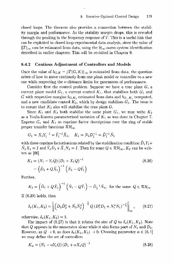
8.4.2 Cautious Adjustment of Controllers and Models

Once the value of bG,K = IIT(G, K)lloo is estimated from data, the question arises of how to move cautiously from one plant model or controller to a new one while respecting the v-distance limits for guarantees of performance.

Consider first the control problem. Suppose we have a true plant G, a current plant model G 1, a current control K 1, that stabilises both Gland G with respective margins bG,K1 estimated from data and bG1,K1 computed, and a new candidate control K 2 , which by design stabilises Gl . The issue is to ensure that K2 also will stabilise the true plant G.

Since Kl and K2 both stabilise the same plant Gl , we may write K2 as a Youla-Kucera parameterised variation of Kl as was done in Chapter 7. Express Gl and Kl as coprime factor descriptions over the ring of stable proper transfer functions RHoo

-1 - -1 - -1 - -1 -Gl = XlYl = Yl Xl, Kl = NIDI = Dl Nl

with these coprime factorisations related by the stabilisation condition Ih Yl + NlXl = I and i\Dl +XlNl = I. Then for some Q E RHoo , K2 can be writ­ten as [66]

K2 = (Nl - YlQ) (Dl + XlQ)-l (8.26)

= (fh +QX1)-1 (N1 -QY1)

Further,

K2 = (Ih + QXl) -1 (Nl - QYl ) = Ix; 1 N2 , for the same Q E RHoo

If (8.20) holds, then

dv(Kl' K2) = II (D2D~ + N2N;) -~ Q (DrDl + Nt Nd-~ 1100' (8.27)

otherwise, dv(Kl' K 2 ) = 1. The impact of (8.27) is that it relates the size of Q to dv(Kl,K2)' Note

that Q appears in the numerator alone while it also forms part of N2 and D2. However, as Q --+ 0, so does dv(Kl' K2) --+ O. Choosing parameter a E (0,1] we may define the set of controllers

(8.28)

180 R.R. Bitmead

This is a set of controllers, all of which stabilise the model GI and which varies continuously from KI at a = 0 to K2 at a = 1. Given stability margin bC,K1 > 0, there always exists an ao > 0 such that

With this construction, it is possible to take an existing stabilising con­troller KI with margin bC,K1 and a candidate controller K2 (usually designed without any connection to KI in mind) and to produce a new composite con­troller K cx , which has guaranteed stability and performance properties. By exchanging the places of plant models and controllers above, a related ap­proach may be generated that commences with current model G I stabilised by K2 and candidate model G2 also selected to be stabilised by K 2, so that it generates a class of plant models parameterised by a Youla-Kucera parameter R times scalar (3 E (0,1]. We might then choose G(3 so that satisfies

for some constant 'Y. In this way, the model movement may also be cau­tiously regulated. These constructions of close models and controllers have been discussed more extensively in [24].

8.4.3 Simultaneous Cautious Controller and Model Adjustment

Iterative identification and control design combines many ingredients; no­tably a true plant G, an initial controller Ko, and sequences of plant models {Cd and controllers {Ki}' The simultaneous stabilisation property exhib­ited by these sets is that each plant model, GHI , is stabilised by the pair of controllers Ki and K HI . Each controller, K i, stabilises the pair of plant models G i and GiH . This is illustrated in Figure 8.2. It should be pointed

p o

/

C o /,

Control Design

Model Control Fitting Design

"'/ P J

C 1

Model Fitting

'" P 2

Fig. 8.2. Simultaneous stabilisation diagram for joint modelling and control design. Directed arrows indicate stabilisation.

out that underlying this simultaneous stabilisation of GiS and Kis is the sta­bilisation and closed-loop performance of G by the KiS. The question arises

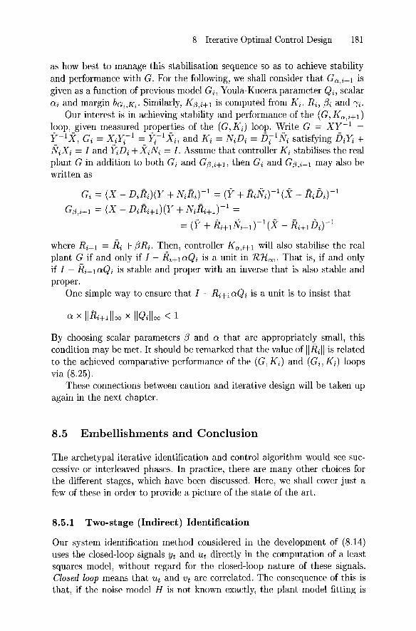
8 Iterative Optimal Control Design 181

as how best to manage this stabilisation sequence so as to achieve stability and performance with G. For the following, we shall consider that Ga,i+l is given as a function of previous model Gi, Youla-Kucera parameter Qi, scalar O:i and margin bOi,Ki' Similarly, K{3,i+1 is computed from K i , Ri, (3i and "ii.

Our interest is in achieving stability and performance of the (G, K a, i+l )

loop, given measured properties of the (G, K i) loop. Write G = Xy-1 = - - 1 - 1- - 1- -y-1 X, Gi = Xi~- = ~- Xi, and Ki = NiDi = Di Ni satisfying DXi + NiXi = I and fiDi + fCNi = I. Assume that controller Ki stabilises the real plant G in addition to both G i and G{3,i+l, then G i and G{3,i+1 may also be written as

where Ri+1 = Ri + (3Ri. Then, controller K a ,i+1 will also stabilise the real plant G if and only if I - Ri+l o:Q i is a unit in RHoo. That is, if and only if I - Ri+lo:Qi is stable and proper with an inverse that is also stable and proper.

One simple way to ensure that 1- Ri+lo:Qi is a unit is to insist that

By choosing scalar parameters (3 and 0: that are appropriately small, this condition may be met. It should be remarked that the value of IIRil1 is related to the achieved comparative performance of the (G, K i ) and (G i , K i ) loops via (8.25).

These connections between caution and iterative design will be taken up again in the next chapter.

8.5 Embellishments and Conclusion

The archetypal iterative identification and control algorithm would see suc­cessive or interleaved phases. In practice, there are many other choices for the different stages, which have been discussed. Here, we shall cover just a few of these in order to provide a picture of the state of the art.

8.5.1 Two-stage (Indirect) Identification

Our system identification method considered in the development of (8.14) uses the closed-loop signals Yt and Ut directly in the computation of a least squares model, without regard for the closed-loop nature of these signals. Closed loop means that Ut and Vt are correlated. The consequence of this is that, if the noise model H is not known exactly, the plant model fitting is

182 R.R. Bitmead

bia'sed by the correlated noise. This can be seen in (8.14) through the plant model dependence on the second Pv term.

A method to yield an unbiased plant model has been suggested by Van den Hof and Schrama [147]. Here, a model is first fitted between the external reference signal rt and the input Ut. Since the input to this fit, rt, is indepen­dent from the noise, which is a filtered version of Vt, this yields an unbiased model. Also, because this model will not be used for anything but filtering, the model structure can be selected with very high order without penalty. We may write

Ut = t[J(z)rt + Y(z)et

Now, the artificial signal, ur = t[J(z)rt, can be computed by filtering di­rectly rt. This new signal is the part of Ut that is caused by rt and is au­tomatically independent from the process disturbance Vt. A plant model is then fitted

Yt = G(z)ur + H(z)et

without bias problems. There are connections between this two-stage identi­fication, with its stable filtering of the data by a nominal closed-loop, and the dual-Youla or Hansen scheme developed in conjunction with the Windsurfer scheme of Chapter 7.

Unbiased models of the actual plant need not necessarily be the ideal out­come, however. Especially with reduced order or approximate system models, one still must ensure that the fit is connected to the ultimate application requirements. This is discussed in [108]. For the sugar mill control design problem of Chapter 13, however, because of the rather dominant nature of the disturbance process over the excitation, two-stage identification was an important step in refining the model [125].

8.5.2 Performance Robustness Versus Stability Robustness

The selection of controller tuning above sought to do two things:

• to force the designed controller to yield good achieved performance, per­haps at the expense of the designed performance;

• to keep the plant and model performances close with the same controller ki ;

Performance was the dominant agenda and no attempt was made to ensure that stability guarantees were respected.

There are different approaches to achieve this latter objective, although usually at some expense to the former.

Robustness of global objective: If one recognizes the reliance on models of these design methods, iteration notwithstanding, it is prudent to include

8 Iterative Optimal Control Design 183

some robustness requirement in the formulation of the global objective crite­rion. For LQG, this is not as simple as some other methods, but a stability robustness check ought to form part of the acceptance conditions for a con­troller. Connections are studied in [46].

Identification for stability robustness: Instead of selecting the performance-oriented modelling criterion of LlP, one might as well choose (8.1). This leads to a different choice of reference spectrum and data filter L, see [161].

Controller validation test: At each new control design phase, it is possible to perform sufficient tests to guarantee whether the controller will stabilise the real plant. The work of Vinnicombe [153] provides a measure of permissi­ble (Ki' Ki+l) controller variation in terms of the currently achieved (G, K i ) performance. Both the performance and the variation are measured using frequency domain tools. This leads to the application of cautious techniques of controller update [7,24,25]. Other statistical tests may be performed to verify that the plant belongs to the set of systems stabilised by the controller.

8.5.3 1£00 Variants

In order to achieve guaranteed robustness margins, one is tempted to translit­erate these techniques from the L2 framework to 1ioo . However, there are still significant problems to be overcome in the formulation of 1ioo system iden­tification in such a way that it links properly to the excited experiment and the control objective. This is discussed by Bayard et al. [20] and [161]. One feature of the 1ioo schemes not enjoyed by LQG-Least squares is that a truly decrescent algorithm is possible with both identification and control design having identical criteria.

8.5.4 Model-free Controller Tuning

Hjalmarsson et al. [78] and Kammer et al. [95] both consider the tuning of controllers using closed-loop experimental data but without the introduction of an explicit plant model. They use direct estimates of the gradient and Hessian of the control criterion based on the signal measurements. This has the advantage of not involving a modelling phase at all, but it is capable only of convergence to a local minimum. These methods are designed for use with restricted complexity controllers, such as PID controllers.

8.5.5 Conclusion

One view of iterative identification and control design is that it is a variety of adaptive control. Indeed, if one were to conduct adaptive control with the controller update not occurring until the end of an experiment, one would

184 R.R. Bitmead

have a similar tactic to these iterative methods. Whereas adaptive control has proven surprisingly difficult to apply in many different practical prob­lems, iterative identification and control has met with a number of early successes. One would expect that a range of profitable connections remain to be established between these related approaches.

Areas in which results still are very much needed include experiment design, where the selection of excitation spectrum iPr is linked to the ultimate goal, and model structure selection, where plant and noise model complexity need to be matched to the control objective. There is still a large number of open problems for this promising area. Other source material is available in [60,69,102,106,161].

Acknowledgements

The author acknowledges the valuable inputs to this work of Brian Anderson, Michel Gevers, Leonardo Kammer, Ari Partanen and Zhuquan Zang. Research supported by US National Science Foundation under Grant ECS-0070146.