iterative and core-guided maxsat solving a survey...

Iterative and Core-Guided MaxSAT Solving

A Survey and Assessment

Antonio Morgado1, Federico Heras1, Mark Liffiton3, Jordi Planes2, and Joao Marques-Silva1

1 CSI/CASL, University College Dublin

{ajrm,fheras,jpms}@ucd.ie2 Universitat de Lleida

[email protected] Illinois Wesleyan University, Bloomington, IL, USA

[email protected]

Abstract. Maximum Satisfiability (MaxSAT) is an optimization version of SAT, and many real world appli-

cations can be naturally encoded as such. Solving MaxSAT is an important problem from both a theoretical

and a practical point of view. In recent years, there has been considerable interest in developing efficient al-

gorithms and several families of algorithms have been proposed. This paper overviews recent approaches to

handle MaxSAT and presents a survey of MaxSAT algorithms based on iteratively calling a SAT solver which

are particularly effective to solve problems arising in industrial settings.

First, classic algorithms based on iteratively calling a SAT solver and updating a bound are overviewed. Such

algorithms are referred to as iterative MaxSAT algorithms. Then, more sophisticated algorithms that addition-

ally take advantage of unsatisfiable cores are described which are referred to as core-guided MaxSAT algo-

rithms. Core-guided MaxSAT algorithms use the information provided by unsatisfiable cores to relax clauses

on demand and to create simpler constraints.

Finally, a comprehensive empirical study on non-random benchmarks is conducted, including not only the

surveyed algorithms, but also other state-of-the-art MaxSAT solvers. The results indicate that (i) core-guided

MaxSAT algorithms in general abort in less instances than classic solvers based on iteratively calling a SAT

solver and that (ii) core-guided MaxSAT algorithms are fairly competitive compared to other approaches.

1 Introduction

The Satisfiability problem in propositional logic (SAT) is the task of deciding whether a given propositional for-

mula has a model. MaxSAT is an optimization variant of SAT and it can be seen as a generalization of the SAT

problem. Given a propositional formula in conjunctive normal form (CNF), the objective of the MaxSAT problem

is to find an assignment for the Boolean variables that maximizes the number of satisfied clauses.

In weighted MaxSAT, each clause has an associated weight and the goal becomes maximizing the sum of the

weights of the satisfied clauses. In many problems originated from real world domains, a subset of the clauses

must be satisfied (denoted hard clauses), and the remaining (soft) clauses may be satisfied or not. Weights are

usually modeled as natural numbers, and hard clauses are modeled by giving each a sufficiently large weight [28].

There are several variants of the MaxSAT problem [28] depending on the distribution of soft and hard clauses.

When all clauses are soft and their weight is 1, the problem is referred to as unweighted MaxSAT. When all clauses

are soft and some weights are greater than 1, it is referred to as weighted MaxSAT. When all soft clauses have

weight 1 and there is a set of hard clauses, it is referred to as partial MaxSAT. Finally, when some soft clauses

have a weight greater than 1 and there is a set of hard clauses, it is referred to as weighted partial MaxSAT. For all

MaxSAT variants, this paper considers the cost of a given truth assignment (whether an optimal solution or not) to

be the sum of the weights of the clauses not satisfied by that assignment. The goal of every variant is thus to find

an assignment with minimum cost.

The remainder of this section is organized as follows. First, the applications of MaxSAT are presented, fol-

lowed by an overview of the existing MaxSAT algorithms in the literature. Then, a general description of the

MaxSAT algorithms surveyed in this paper is given, and the section ends with the goals and structure of the

survey.

1.1 MaxSAT Applications

Many important problems can be naturally expressed as MaxSAT. These include academic problems such as

Max-Cut or Max-Clique, as well as problems from many industrial domains. Concrete examples inclde the fol-

lowing domains Routing problems [117]; in different problems of Bioinformatics, such as Protein Alignment [111],

Haplotyping with Pedigrees [51], Reasoning over Biological Networks[53]; in Hardware Debugging, both on De-

sign Debugging [102], as well as on Circuit Debugging [76, 31]; in Software Debugging (of C code) [61, 62]; in

Scheduling [115]; in Planning [34, 63, 118, 99]; in Course Timetabling [15, 16]; in Probabilistic Reasoning [94];

in Electronic Markets [103]; in Credential-Based interactions as a way to minimize the disclosure of private infor-

mation [11]; in Enumeration of MUSes/MCSes [73, 98, 24]; in Software Package Upgrades [75, 114, 13, 14, 12];

in Combinatorial Auctions [55]; in Quantified Boolean Formulas [27].

Additionally, MaxSAT algorithms have also been successfully applied as a way to compute the Binate/Unate

Covering problem, where it has been applied to Haplotype Inference [52], to Digital Filter Design [1], to FSM

Synthesis and Logic Minimization, [54], among others. Analogously, many problems originally formulated in

other optimization frameworks can be easily reformulated as MaxSAT including the Pseudo-Boolean Optimization

framework [3], the Weighted CSP framework [68] and the MaxSMT framework [89].

1.2 MaxSAT Algorithms

The last two decades have witnessed significant progress in the development of theoretical and practical work on

MaxSAT. Early theoretical MaxSAT research provided insights in the complexity of the problem [93, 50, 19].

Early practical works on MaxSAT were based on stochastic local search (SLS) [107, 106, 60] with the objective

of approximating the MaxSAT solution. SLS algorithms randomly compute an initial assignment of the variables,

and at each iteration the value of one variable is flipped (from true to false or vice-versa) in a process that attempts

to find an assignment satisfying more clauses than the best found thus far. SLS algorithms do not guarantee to

find the optimal solution and for this reason are referred to as incomplete algorithms. Whereas the mentioned SLS

algorithms were initially developed for the SAT problem, they can be directly applied to approximate (unweighted)

MaxSAT and for the most general Weighted Partial MaxSAT [28]. A recent survey on SLS algorithms can be found

in [59]. Additionally, the most successful SLS algorithms for SAT have been extended for approximating MaxSAT

in the UBCSAT system [113]. SLS has been shown to be among the most effective algorithms to solve randomly

generated problems, but recent work on semidefinite programming has been shown to be quite promising for

approximating random Max2Sat instances [49, 5].

In the last decade, different complete (or exact) algorithms have been proposed for solving MaxSAT to opti-

mality. Some of the existing approaches are based on reducing the MaxSAT problem into a well-known optimiza-

tion problem and then use an off-the-shelf solver for such problem. For example, a natural approach to solve the

MaxSAT problem is to model it as a Integer Linear Program (ILP). The ILP problem can then be solved directly

by a dedicated solver such as CPLEX. Indeed, a ILP problem restricted to 0-1 inequalities (pseudo-Boolean con-

straints) is usually referred to as Pseudo-Boolean Optimization problem [21, 101]. Several approaches have been

2

developed to handle the PBO problem. Most of the existing PBO algorithms, either adapt a modern SAT solver

to natively handle pseudo-Boolean constraints [3, 29, 108] or directly solve a sequence of SAT problems [41]. In

both cases, the aim is to take advantage of modern SAT solvers with powerful clause learning and backjumping

techniques [110, 86, 40].

Another example of reducing MaxSAT includes the Answer Set Programming (ASP) [45], in particular its

optimization version MaxASP [44]. Recent algorithms for MaxASP include a branch and bound approach [91]

and the adapted versions of some core-guided MaxSAT algorithms presented in this survey [4]. The last relevant

reduction include the Weighted Constraint Satisfaction Problem (WCSP). In [38] MaxSAT was represented as a

WCSP for the first time. Current solving approaches for WCSP are based on branch and bound algorithms which

apply local consistency to boost the search [35], as well as stochastic local search approaches [87].

Besides reductions, other approaches are based on adapting a modern SAT solver by either (i) forcing an order

on the selection of variables during the search, that by construction leads to the optimal solution [47, 46, 100], or

(ii) by integrating knowledge compilation-based lower bounds and exploiting them during the search [97, 95].

A large family of contemporary exact MaxSAT solvers follow a branch and bound (BB) algorithm [26, 116,

71, 67, 56, 92, 37]. BB algorithms assign a variable at each node of a search tree, simplify the current formula

and compute lower bounds and upper bounds on the value of any assignment that may be found below that node.

Whenever the lower bound matches the upper bound, no solution better than the current one can be found in that

branch, and the algorithm can backtrack.

The first branch and bound MaxSAT algorithm was proposed in [26], which is organized in two phases. In

the first phase, a SLS algorithm is used to compute an initial upper bound. Then, in a second phase, the actual

branch and bound takes place in which primitive lower bounds and simplification rules were applied at each of the

nodes of the search tree. Later works added more effective techniques in order to boost the search. Namely, more

efficient data-structures, new branching heuristics, new simplification rules and more accurate lower bounds [88,

112, 109, 116]. Modern BB solvers additionally exploit unit propagation [70] to compute powerful lower bounds,

as well as new inference rules [71, 67, 56] based on the resolution rule for MaxSAT [66, 25, 67]. Those algorithms

have been recently surveyed in [69] and are particularly effective on random and crafted benchmarks.

Another large family of MaxSAT algorithms is based on iteratively calling a SAT solver. Those algorithms

are particularly suitable for benchmarks coming from industrial settings. This paper presents a survey on those

algorithms which are characterized by adding fresh relaxation variables to soft clauses, adding a set of cardinality

or pseudo-Boolean constraints to the formula, and then sending the resulting formula to a SAT solver. The next

subsection briefly introduces MaxSAT algorithms based on iteratively calling a SAT solver.

1.3 Iterative and core-guided MaxSAT Algorithms

Early theoretical works [93, 50] introduced linear search and binary search in order to characterize the complexity

of the MaxSAT problem and other optimization problems. Those algorithms initially relax all soft clauses and use

cardinality/pseudo-Boolean constraints [41] (at most constraints AtMostK) to refine a given (lower or upper)

bound. Algorithms based on linear search can be of one of two main variants: those that refine an upper bound on

the value of the optimum solution, and those that refine a lower bound.

Algorithms that iteratively refine upper bounds will be referred to as linear search Sat-Unsat, denoting that all

calls to the SAT solver but the last will declare the given formula as satisfiable. Several MaxSAT tools are available

that follow a linear search Sat-Unsat strategy, for example SAT4J [22] and QMAXSAT [64]. Note that using a SAT

solver following linear Sat-Unsat scheme has also been used in other domains, for example in the PBO solvers

PBS [2], MINSAT+ [41] and SAT4J [22].

3

Algorithms that iteratively refine lower bounds will be referred to as linear search Unsat-Sat, denoting that

all calls to a SAT solver but the last will return unsatisfiable. There are no known implementations of the linear

search Unsat-Sat algorithm specifically for MaxSAT, though CAMUS [72], which computes minimal unsatisfiable

subsets (MUS) of an input formula, does use such an approach in its first phase, solving MaxSAT as a side-effect

of its primary goal.

A different strategy consists in applying binary search [43] to find the optimal solution. Binary search main-

tains both a lower bound and an upper bound. Essentially, it computes the midpoint between the upper and lower

bounds and calls a SAT solver to test whether there exists a solution whose value is less than or equal to the

midpoint. If the SAT solver returns satisfiable, the upper bound can be updated to the value of the model found.

Alternatively, if the solver returns unsatisfiable, the lower bound can be updated to the middle value just tested.

Observe that, in the worst case, binary search requires a number of calls to the SAT solver linear in the problem

size (the number of soft clauses), whereas linear search may require an exponential number of calls. A MaxSAT

solver that follows the binary search scheme was introduced in [43]. Also, one of the algorithms introduced in

[64] alternates binary search and linear search Sat-Unsat at each iteration. In [32] binary search was used to solve

an optimization version of the SMT framework. Bit-based search [33, 48] aims to find the optimal solution by

exploring its binary representation and also requires a linear number of calls to a SAT. A prolog implementation

was proposed in [33] for bit-based search.

The algorithms described so far require the SAT solver to report the satisfiable (SAT) or unsatisfiable (UNSAT)

outcomes and to provide models on SAT outcomes. Additionally, such algorithms relax all soft clauses before

calling the SAT solver for the first time. Those algorithms are referred to as iterative MaxSAT algorithms.

More recent algorithms based on iteratively calling a SAT solver take advantage of the information provided by

unsatisfiable cores [119] to guide the search. Such algorithms are referred to as core-guided MaxSAT algorithms.

Hence, core-guided MaxSAT additionally require the SAT solver to be able to produce unsatisfiable cores on

UNSAT outcomes. In particular, unsatisfiable cores are used to relax soft clauses on demand and/or to create

constraints which are shorter in the sense that involve a smaller set of relaxation variables. Existing core-guided

MaxSAT algorithms follow an algorithmic scheme similar to linear or binary search.

The seminal core-guided algorithm was introduced in [43] (referred in this paper as MSU1), which was restricted

to unweighted partial MaxSAT. At each iteration, a relaxation variable is added to each soft clause involved in

a newly extracted unsatisfiable core, and a new constraint is added to the formula. Several improvements were

introduced later in MSU1.1 [80], MSU1.2 [79], and its weighted version was simultaneously presented in [77] and

[8] (respectively, WMSU1 and WPM1). Both WMSU1 and WPM1 [43] algorithms may require more than one relaxation

variable per soft clause and use AtMost1 constraints (instead of general AtMostK constraints).

More recent algorithms relax soft clauses on demand, add at most one relaxation variable per soft clause and

use general AtMostK constraints. MSU3 was the first algorithm to follow such organization and it is based on

refining a lower bound. Similarly, PM2 and PM2.1 also refine a lower bound and add additional constraints to

the formula based on a heuristic that counts how many previous unsatisfiable cores are contained at each new

unsatisfiable core. PM2.1 is the first algorithm to take advantage of disjoint cores (or covers) to add smaller

constraints to the formula. Essentially, a disjoint core is an unsatisfiable core that does not share any soft clause

with previous unsatisfiable cores. A weighted version of PM2.1 can be found in WPM2 [9]. WPM2 introduced a

technique based on the subset sum problem to refine the lower bound at each iteration. A simplified version of

such technique is borrowed in this paper to extend several iterative and core-guided MaxSAT algorithms, which

were originally presented in their unweighted version, to handle weighted clauses.

MSU4 [81] alternates satisfiable and unsatisfiable calls to the SAT solver and also relaxes soft clauses on de-

mand. Core-guided binary search [58] relaxes soft clauses on demand and follows a binary search strategy. Finally,

4

core-guided binary search with disjoint cores [58] enhances the previous algorithm by maintaining disjoint cores.

Note that WMSU4 and both versions of core-guided binary search refine both a lower bound and an upper bound.

Note that several works have been proposed to handle other optimization problems using similar or adapted

versions of the iterative and core-guided MaxSAT algorithms presented so far. As mentioned before, linear search

Sat-Unsat has been widely used for PBO and an adapted version of MSU1 and MSU3 for MaxASP [4]. Additionally,

several works have been recently presented to handle an optimization version of the Satisfiability Modulo Theories

(SMT) framework, referred in this paper as MaxSMT. Such works include [90, 20, 105] to name a few. In this

paper, it is explained how iterative and core-guided MaxSAT algorithms can be easily adapted to handle the

MaxSMT problem.

Contemporary MaxSAT algorithms are based not only on iteratively calling a SAT solver to retrieve models

or unsatisfiable cores, but also require the integration of additional sophisticated techniques. Such approaches in-

clude an algorithm [36] that uses linear programming technology to handle the cardinality and pseudo-Boolean

constraints, more aggressive computation of lower bounds and upper bounds at each disjoint core for the core-

guided binary search with disjoint cores algorithm [85], and the integration of several techniques in WMSU1, in-

cluding Boolean multilevel optimization [78] , MaxSAT resolution [57], breaking symmetries [6], partitioning

soft clauses [82].

1.4 Goals and Structure

The main goal of this paper is to present a survey of iterative and core-guided MaxSAT algorithms. Some of the

algorithms were originally introduced in their unweighted version. In this paper, these algorithms are extended

to handle weighted partial MaxSAT. In particular, a total of 14 algorithms are described in detail and character-

ized by several properties. Such algorithms were implemented in the same software platform so that they could

be fairly compared in order to better understand which are the most competitive algorithms independently of

implementation details. A comprehensive empirical study was conducted including not only the algorithms de-

scribed in this paper but also other state-of-the-art MaxSAT solvers. The results on non-random benchmarks from

MaxSAT Evaluations indicate that (i) core-guided MaxSAT algorithms in general abort in fewer instances than

classic algorithms based on iteratively calling a SAT solver and that (ii) core-guided MaxSAT algorithms are fairly

competitive compared to the other approaches.

The paper is structured as follows. Section 2 formally defines the MaxSAT problem and related notation,

as well as preliminary notation that will be used when describing MaxSAT algorithms (Section 2.3). Iterative

MaxSAT algorithms are introduced in Section 3 and core-guided algorithms in Section 4. Section 5 presents the

MaxSMT problem, which can be seen as a generalization of the MaxSAT problem, and shows how current SMT

solvers can be easily turned into MaxSMT solvers implementing any of the algorithms described in this survey.

The experimental investigation is shown in Section 6. Finally, Section 7 presents some concluding remarks.

2 Preliminaries

This section presents the necessary definitions and notation related to the SAT and MaxSAT problems, as well as

the notation used for describing the MaxSAT algorithms throughout the paper.

2.1 Boolean Satisfiability (SAT)

Let X = {x1, x2, . . . , xn} be a set of Boolean variables. A literal is either a variable xi or its negation ¬xi. The

variable to which a literal l refers is denoted by var(l). Given a literal l, its negation ¬l is ¬xi if l is xi and it is

5

xi if l is ¬xi. A clause c is a disjunction of literals. Hereafter, lower case letters will represent clauses. The size of

a clause, noted |c|, is the number of literals it contains. A formula in conjunctive normal form (CNF) ϕ is a set of

clauses. An assignment is a set of literals A = {l1, l2, . . . , ln} such that for all li ∈ A, its variable var(li) = xi

is assigned to a value (true or false). If variable xi is assigned to true, literal xi is satisfied and literal ¬xi

is unsatisfied (or falsified). Similarly, if variable xi is assigned to false, literal ¬xi is satisfied and literal xi is

unsatisfied. If all variables in X are assigned, the assignment is called complete, otherwise it is called partial. An

assignment satisfies a literal iff it belongs to the assignment, it satisfies a clause iff it satisfies one or more of its

literals and it unsatisfies a clause iff it contains the negation of all its literals. The empty clause, noted ✷, has no

literals (size 0) and cannot be satisfied.

A model is a complete assignment that satisfies all the clauses in a CNF formula ϕ. SAT is the problem of

deciding whether there exists a model for a given propositional formula. Given an unsatisfiable SAT formula ϕ, a

subset of clauses ϕC whose conjunction is still unsatisfiable is called an unsatisfiable core of the original formula.

Given an unsatisfiable formula, modern SAT solvers can be instructed to generate an unsatisfiable core [119].

2.2 Maximum Satisfiability (MaxSAT)

A weighted clause is a pair (ci, wi), where ci is a clause and wi is the cost of falsifying it, also called its weight.

Many real problems contain clauses that must be satisfied. Such clauses are called mandatory (or hard) and are

associated with a special weight ⊤. Note that any weight wi ≥ ⊤ indicates that the associated clause must be

necessarily satisfied. Thus, wi can be replaced by ⊤ without changing the problem. Consequently, all weights

take values in {0, . . . ,⊤}. Non-mandatory clauses are also called soft clauses. A formula in weighted conjunctive

normal form (WCNF) ϕ = ϕH ∪ ϕS is a set of weighted clauses where ϕH is the set of hard clauses, and ϕS is

the set of soft clauses.

A model is a complete assignment A that satisfies all mandatory clauses. The cost of a model is the sum of

weights of the soft clauses that it falsifies. Given a WCNF formula ϕ = ϕH ∪ ϕS , Weighted Partial MaxSAT

is the problem of finding a model of minimum cost. In other words, the objective is to find an assignment that

satisfies all hard clauses in ϕH and minimizes the sum of weights of unsatisfied soft clauses in ϕS . If the set of

hard clauses is empty (ϕH = ∅), the problem is called weighted MaxSAT problem. When all the weights are equal

to 1 (∀i : wi = 1), then the problem is called partial MaxSAT problem. Finally, if both the set of hard clauses

is empty (ϕH = ∅), and all the weights are equal to 1 (∀i : wi = 1), then the problem is called (unweighted)

MaxSAT problem.

2.3 Describing MaxSAT Algorithms

The algorithms described in this paper are based on iteratively calling a SAT solver. At each iteration, the algorithm

creates a CNF instance and invokes a SAT solver on it. Depending on the result given by the SAT solver, the

algorithm updates the CNF formula accordingly and starts a new iteration. Two types of algorithms are considered

in this paper: Iterative MaxSAT algorithms that on each iteration update a bound depending on the result returned

by the SAT solver (satisfiable or unsatisfiable) and core-guided MaxSAT algorithms that additionally exploit the

information in the unsatisfiable cores returned by the SAT solver on unsatisfiable outcomes.

All the algorithms make use of relaxation variables. Relaxation variables are new Boolean variables that are

added to the soft clauses of the formula. Unless otherwise indicated, the algorithms associate at most one unique

relaxation variable with each soft clause. In terms of notation, relaxation variables are maintained in a set R, and

the relaxation variable ri is associated to the clause ci with weight wi where 1 ≤ i ≤ m. This paper assumes that

any weighted formula ϕ has m soft clauses.

6

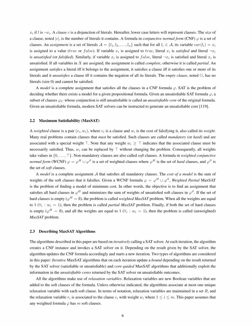
Function RelaxCls(R, ϕ, ψ)

Input: (R,ϕ, ψ) denotes the set of relaxation variables R, and two WCNF formulas ϕ and ψ satisfying ψ ⊆ ϕ1 begin

2 (Ro, ϕo)← (R,ϕ) /* Ro set of relaxation variables; ϕo set of clauses to return */

3 foreach (c, ω) ∈ Soft (ψ) do

4 Ro ← Ro ∪ {r} /* r is a fresh relaxation variable */

5 cR ← c ∪ {r}6 ϕo ← ϕo \ {(c, ω)} ∪ {(cR, ω)} /* (cR, ω) is tagged soft */

7 end

8 return (Ro, ϕo)

9 end

Algorithm 1: MaxSAT Wrapper Algorithm

Input: (ϕ,MSAlgorithm,UBHeuristic, LBHeuristic)1 st← SAT(Hard(ϕ))

2 if st = UNSAT then return ∅ /* No Solution */

3 if UBHeuristic = NIL ∧ LBHeuristic = NIL then return MSAlgorithm(ϕ)4 (A, µ)← UBHeuristic(ϕ)5 (λ, ϕcores)← LBHeuristic(ϕ)6 return MSAlgorithm(ϕ,A, µ, λ, ϕcores)

In order to add relaxation variables to soft clauses, the algorithms use function RelaxCls(R,ϕ, ψ), which

receives a set of relaxation variablesR, a WCNF formula ϕ, and a set of soft clauses ψ. It returns the pair (Ro, ϕo),

where ϕo corresponds to a copy of ϕ whose soft clauses included in ψ have been augmented with fresh relaxation

variables, and Ro corresponds to R augmented with the relaxation variables added in ϕo. See the pseudo-code in

Function RelaxCls.

Given the set of relaxation variables R, the algorithms add cardinality / pseudo-Boolean constraints [43] and

translate them to hard clauses. Such constraints usually state that the sum of the weights of the relaxed clauses

is bounded above (AtMostK constraint with∑m

i=1 wiri ≤ K) or bounded below (AtLeastK constraint with∑m

i=1 wiri ≥ K) by a specific value K.

Opt(ϕ) will refer to the optimal solution of instance ϕ. The algorithms may use the following variables: λ for

a lower bound, µ for an upper bound, ν for the value the algorithm is searching (in the current iteration), and ι for

one bit of the binary representation of that value. The algorithms also make use of the following functions:

– Soft(ϕ) returns the set of all soft clauses in ϕ.

– Hard(ϕ) returns the set of all hard clauses in ϕ.

– SAT (ϕ) makes a call to the SAT solver which returns whether ϕ is satisfiable (SAT) or unsatisfiable (UN-

SAT). The SAT solver returns a complete assignment A if ϕ is satisfiable, otherwise A is empty. When ϕ is

unsatisfiable, the SAT solver is able to return an unsatisfiable core ϕC .

– CNF (c) returns a set of clauses that encode the pseudo-boolean constraint c into CNF.

– Init(A) , given the assignment A, returns the set of assignments in A to the initial variables of the input

formula ϕ.

Without loss of generality, all the algorithms presented in this paper assume that the input formula is not

empty and that the set of hard clauses of the input formula has a model. In practice, it is expected that a wrapper

checks these assumptions before calling the actual MaxSAT algorithm. The pseudo-code for such a wrapper can

be found in Algorithm 1. The parameters of the wrapper are a WCNF formula (ϕ), the algorithm to execute

(MSAlgorithm) and the upper bound and lower bound heuristic to compute (LBHeuristic and UBHeuristic).

Initially, a SAT solver is called with the hard clauses of the formula (line 1). If the SAT solver returns unsatisfiable,

7

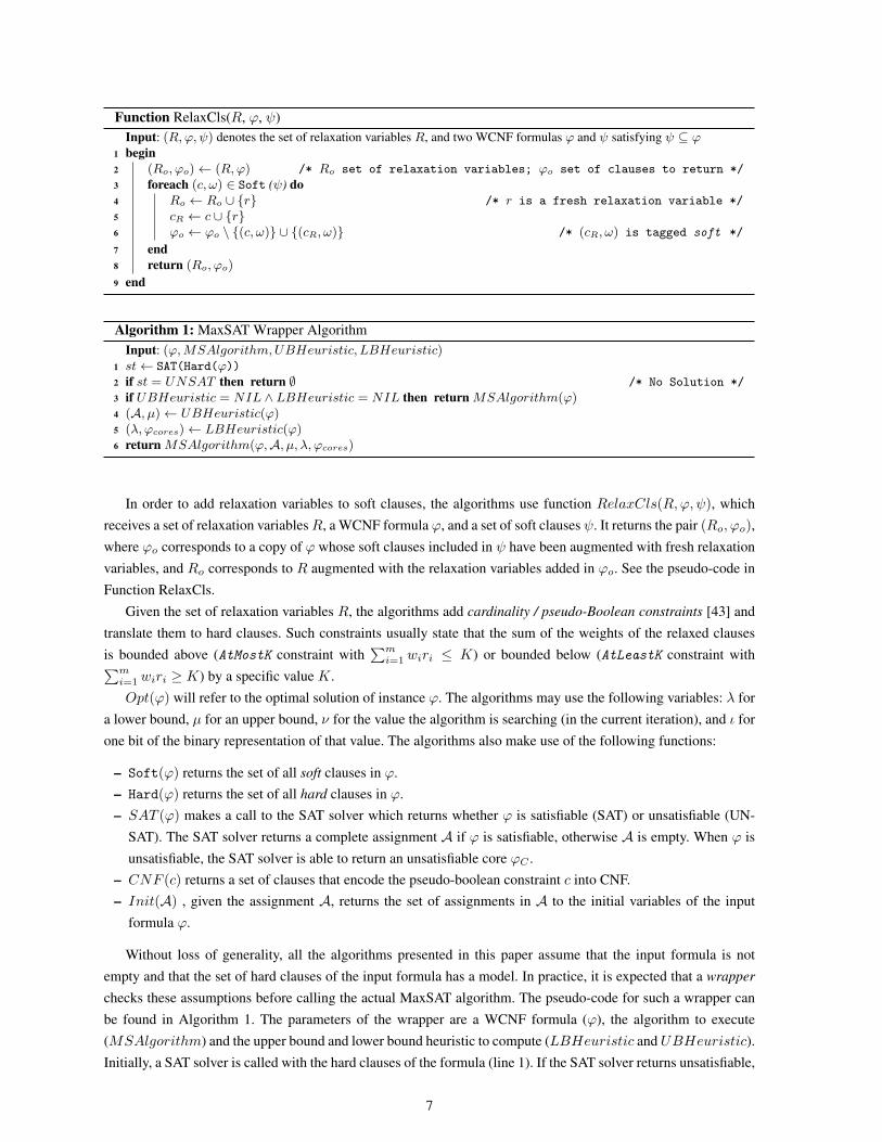
Algorithm 2: LIN-US: The Linear Search Unsat-Sat Algorithm

Input: ϕ

1 (R,ϕW )←RelaxCls(∅, ϕ, Soft(ϕ))2 λ← 03 while true do

4 (st,A)← SAT(Cls(ϕW ) ∪ CNF(∑m

i=1wi · ri ≤ λ))

5 if st = SAT then return Init(A)6 λ← RefineBound({ωi|1 ≤ i ≤ m}, λ)

7 end

Table 1. Running example for the Linear Unsat-Sat Algorithm. #i represents the i-th iteration of the algorithm.

ϕW = {(x1 ∨ r1), (x2 ∨ r2), (x3 ∨ r3), (x4 ∨ r4), (x5 ∨ r5), (x6 ∨ r6), (¬x6 ∨ r7)} ∪ ϕH

λ = 0;

#1Constraint to include: CNF(r1 + r2 + r3 + r4 + r5 + r6 + r7 ≤ 0)st = UNSAT;

λ = 1;


λ = 2;


λ = 3;


λ = 4;

#5Constraint to include: CNF(r1 + r2 + r3 + r4 + r5 + r6 + r7 ≤ 4)st = SAT;

Init(A) = {x3 = x5 = 1;x1 = x2 = x4 = x6 = 0}

it means that the problem has no solution (line 2). Otherwise, the specific MaxSAT solver is called in line 3. If an

upper bound or a lower bound are used, these are computed in lines 4 and 5, and the specified MaxSAT algorithm

is called with the computed bounds in line 6. The MaxSAT algorithms are described in Sections 3 and 4. Lower

and upper bound heuristics are described in detail in [58] and briefly reviewed below.

First, the upper bound µ is described. Each soft clause in ϕ is extended with a new relaxation variable obtaining

a new formula ϕ’. Then, a SAT solver is called with the resulting formula ϕ’ and no additional constraints. Clearly,

a satisfying assignment A exists for ϕ’. Then, the sum of weights of soft clauses which are unsatisfied by A

(disregarding relaxation variables) corresponds to a correct upper bound µ.

The lower bound λ is initially set to 0. The instance is iteratively sent to the SAT solver until a satisfiable

instance is reached. For each unsatisfiable core ϕC , the minimum weight m among the soft clauses in ϕC is added

to the lower bound (λ = λ+m), and each soft clause in ϕC is augmented in ϕ with a fresh relaxation variable.

3 Iterative Algorithms

A straightforward approach for MaxSAT solving using a SAT solver is to iteratively convert the optimization

problem into a decision problem: Given a WCNF formula ϕ, the algorithm checks the satisfiability of ϕ together

with a constraint (expressed in clauses) stating that the sum of weights of unsatisfied clauses equals a given K.

The algorithm starts from its minimum value (K = 0) and increases it up to the optimal solution, or starts from

its maximum value (K =∑m

i=1 wi) and decreases down to the optimal solution.

The Linear Search Unsat-Sat algorithm looks for an optimal solution from unsatisfiable instances until a

satisfiable instance is identified. At every step, the value λ, which is a lower bound on the optimal solution, is

8

increased by one until the solution is found. The pseudo-code of Linear Search Unsat-Sat is shown in Algorithm

2. Initially, all soft clauses are relaxed (line 1) and the lower bound is initialized to 0 (line 2). Then, the main loop

(line 3) iterates while the SAT solver returns unsatisfiable (line 5). At each iteration, the SAT solver is called with

the clauses of the current working formula and the encoding of the AtMostK constraint∑m

i=1 wi · ri ≤ λ (line 4).

Essentially, the AtMostK constraint requires that, for any satisfying assignment, the sum of weights of the clauses

whose relaxation variables are assigned to true is lower or equal to the lower bound λ. If the SAT solver returns

unsatisfiable, the lower bound λ is increased (line 6), otherwise the algorithm terminates (line 5) and returns the

satisfying assignment A restricted to the original variables.

Example 1. Let ϕ = ϕS ∪ ϕH be a partial MaxSAT instance with 6 variables, a set of 7 soft clauses ϕS , where

ϕS = {(x1, 1), (x2, 1), (x3, 1), (x4, 1), (x5, 1), (x6, 1), (¬x6, 1)}, and a set of 5 hard clauses ϕH , where ϕH =

{(¬x1 ∨ ¬x2,⊤), (¬x2 ∨ ¬x3,⊤), (¬x3 ∨ ¬x4,⊤), (¬x4 ∨ ¬x5,⊤), (¬x5 ∨ ¬x1,⊤)}. From here on, in order

to make the examples easier to follow, the weights are removed; assume all weights in the soft clauses are set to

1 and in the hard clauses set to ⊤. If instance ϕ is given to Linear Search Unsat-Sat (Algorithm 2), the sequence

of iterations is as shown in Table 1. The first column of the table shows the number of the iteration, where the

first row is the initial iteration (before any call to the SAT solver). The second column shows the status of some of

the structures of the algorithm, namely for the initial iteration both the working formula ϕW and the lower bound

λ are presented. Since the Linear Search Unsat-Sat algorithm starts by relaxing all soft clauses in the working

formula, then in the initial iteration ϕW is a union of all the hard clauses (ϕH ) together with the set of soft clauses

ϕS already relaxed. For the remaining iterations, it is shown the constraint that together with the working formula

is sent to the SAT solver. Then the result returned by the SAT solver is presented in the st variable, which is

always unsatisfiable (UNSAT) for iterations #1 to #4 and the lower bound is increased by 1. For iteration #5,

the SAT solver reports the formula to be satisfiable (SAT) and the satisfying assignment is shown in the last row of

the table (restricted to the original variables). In the remaining of the paper, examples of the execution for several

algorithms are presented in a similar fashion to this example.

Observe that in the pseudo-code, λ is updated by RefineBound({ωi|1 ≤ i ≤ m}, λ) instead of just by 1.

Function RefineBound() takes as parameters (i) a vector of weights and (ii) a bound, and it returns a refinement

of the given bound. The possible refinements depend on the distribution of the weights. The following refinements

are considered:

– λ← λ+ 1

– λ← SubSetSum({ωi|1 ≤ i ≤ m}, λ) (as suggested in [9])

For unweighted MaxSAT instances (i.e., all weights equal to 1), the bound refinement cannot be better than λ+1.

However, for weighted MaxSAT the bound refinement using the subset sum could save a considerable number

of iterations [9]. Given a set of integers and an integer k, the subset sum problem asks if there is any subset

of integers such that their sum equals k. The subset sum problem is a well-known NP-hard problem which can

be solved by a pseudo-polynomial algorithm, for example, a dynamic programming algorithm [9]. The bound

refinement SubSetSum({ωi|1 ≤ i ≤ m}, λ) receives the current lower bound λ and the set of weights of the soft

clauses, and it returns the next value for λ such that the subset sum is true.

Example 2. Let ϕ be a weighted formula with four soft clauses with weights 1, 2, 3, and 100 and a set of hard

clauses. The only possible values for the optimal solution are in 0, . . . , 6 and in 100, . . . , 106. So, there is no need

to assign λ to any of the values in 7, . . . , 99 for the Linear Search Unsat-Sat algorithm. If the algorithm is fed with

such instance and the bound refinement is just λ+ 1, it will iterate over all the values 0, . . . , 106 in the worst case

(i.e., Opt(ϕ) = 106). Alternatively, using the bound refinement based on the subset sum, it will iterate only over

the values in 0, . . . , 6 and 100, . . . , 106 in the worst case.

9

Algorithm 3: The Linear Sat-Unsat Algorithm

Input: ϕ

1 (R,ϕW )← RelaxCls(∅, ϕ,Soft(ϕ))2 (µ, lastA)← (1 +

∑m

i=1wi, ∅)

3 while true do


i=1wi · ri ≤ µ− 1))

5 if st = UNSAT then return Init(lastA)6 (lastA, µ)← (A, µ− 1)

7 end

Algorithm 4: LIN-SU: The Linear Sat-Unsat Algorithm with Assignment Leap [22]

Input: ϕ

1 (R,ϕW )←RelaxCls(∅, ϕ, Soft(ϕ))2 (µ, lastA)← (1 +

∑m

i=1wi, ∅)

3 while true do

4 (st,A)← SAT(Cls(ϕW )∪ CNF(∑m

i=1wi · ri ≤ µ− 1))

5 if st = UNSAT then return Init(lastA)6 (lastA, µ)← (A,

∑m

i=1wi · (1−A〈ci \ {ri}〉))

7 end

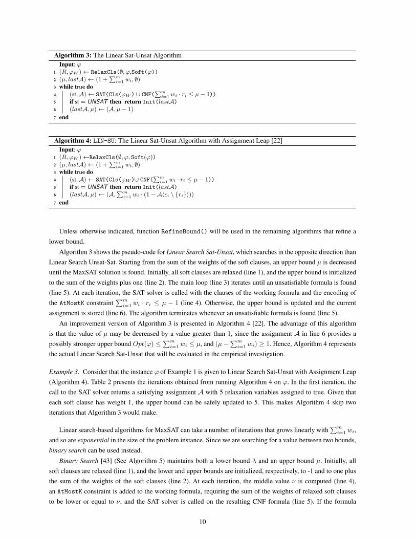
Unless otherwise indicated, function RefineBound() will be used in the remaining algorithms that refine a

lower bound.

Algorithm 3 shows the pseudo-code for Linear Search Sat-Unsat, which searches in the opposite direction than

Linear Search Unsat-Sat. Starting from the sum of the weights of the soft clauses, an upper bound µ is decreased

until the MaxSAT solution is found. Initially, all soft clauses are relaxed (line 1), and the upper bound is initialized

to the sum of the weights plus one (line 2). The main loop (line 3) iterates until an unsatisfiable formula is found

(line 5). At each iteration, the SAT solver is called with the clauses of the working formula and the encoding of

the AtMostK constraint∑m

i=1 wi · ri ≤ µ − 1 (line 4). Otherwise, the upper bound is updated and the current

assignment is stored (line 6). The algorithm terminates whenever an unsatisfiable formula is found (line 5).

An improvement version of Algorithm 3 is presented in Algorithm 4 [22]. The advantage of this algorithm

is that the value of µ may be decreased by a value greater than 1, since the assignment A in line 6 provides a

possibly stronger upper bound Opt(ϕ) ≤∑m

i=1 wi ≤ µ, and (µ−∑m

i=1 wi) ≥ 1. Hence, Algorithm 4 represents

the actual Linear Search Sat-Unsat that will be evaluated in the empirical investigation.

Example 3. Consider that the instance ϕ of Example 1 is given to Linear Search Sat-Unsat with Assignment Leap

(Algorithm 4). Table 2 presents the iterations obtained from running Algorithm 4 on ϕ. In the first iteration, the

call to the SAT solver returns a satisfying assignment A with 5 relaxation variables assigned to true. Given that

each soft clause has weight 1, the upper bound can be safely updated to 5. This makes Algorithm 4 skip two

iterations that Algorithm 3 would make.

Linear search-based algorithms for MaxSAT can take a number of iterations that grows linearly with∑m

i=1 wi,

and so are exponential in the size of the problem instance. Since we are searching for a value between two bounds,

binary search can be used instead.

Binary Search [43] (See Algorithm 5) maintains both a lower bound λ and an upper bound µ. Initially, all

soft clauses are relaxed (line 1), and the lower and upper bounds are initialized, respectively, to -1 and to one plus

the sum of the weights of the soft clauses (line 2). At each iteration, the middle value ν is computed (line 4),

an AtMostK constraint is added to the working formula, requiring the sum of the weights of relaxed soft clauses

to be lower or equal to ν, and the SAT solver is called on the resulting CNF formula (line 5). If the formula

10

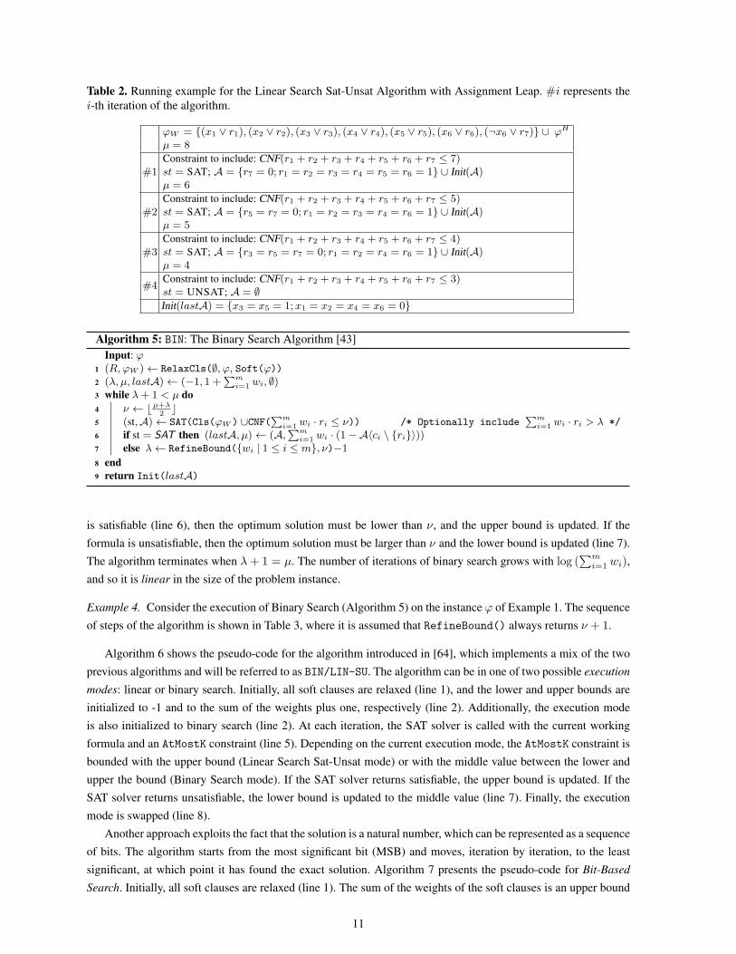
Table 2. Running example for the Linear Search Sat-Unsat Algorithm with Assignment Leap. #i represents the

i-th iteration of the algorithm.


µ = 8

#1Constraint to include: CNF(r1 + r2 + r3 + r4 + r5 + r6 + r7 ≤ 7)st = SAT; A = {r7 = 0; r1 = r2 = r3 = r4 = r5 = r6 = 1} ∪ Init(A)µ = 6

#2Constraint to include: CNF(r1 + r2 + r3 + r4 + r5 + r6 + r7 ≤ 5)st = SAT; A = {r5 = r7 = 0; r1 = r2 = r3 = r4 = r6 = 1} ∪ Init(A)µ = 5

#3Constraint to include: CNF(r1 + r2 + r3 + r4 + r5 + r6 + r7 ≤ 4)st = SAT; A = {r3 = r5 = r7 = 0; r1 = r2 = r4 = r6 = 1} ∪ Init(A)µ = 4

#4Constraint to include: CNF(r1 + r2 + r3 + r4 + r5 + r6 + r7 ≤ 3)st = UNSAT; A = ∅Init(lastA) = {x3 = x5 = 1;x1 = x2 = x4 = x6 = 0}

Algorithm 5: BIN: The Binary Search Algorithm [43]

Input: ϕ

1 (R,ϕW )← RelaxCls(∅, ϕ, Soft(ϕ))2 (λ, µ, lastA)← (−1, 1 +

∑m

i=1wi, ∅)

3 while λ+ 1 < µ do

4 ν ← ⌊µ+λ

2⌋

5 (st,A)← SAT(Cls(ϕW ) ∪CNF(∑m

i=1wi · ri ≤ ν)) /* Optionally include

∑m

i=1wi · ri > λ */

6 if st = SAT then (lastA, µ)← (A,∑m

i=1wi · (1−A〈ci \ {ri}〉))

7 else λ← RefineBound({wi | 1 ≤ i ≤ m}, ν)−1

8 end

9 return Init(lastA)

is satisfiable (line 6), then the optimum solution must be lower than ν, and the upper bound is updated. If the

formula is unsatisfiable, then the optimum solution must be larger than ν and the lower bound is updated (line 7).

The algorithm terminates when λ+ 1 = µ. The number of iterations of binary search grows with log (∑m

i=1 wi),

and so it is linear in the size of the problem instance.

Example 4. Consider the execution of Binary Search (Algorithm 5) on the instance ϕ of Example 1. The sequence

of steps of the algorithm is shown in Table 3, where it is assumed that RefineBound() always returns ν + 1.

Algorithm 6 shows the pseudo-code for the algorithm introduced in [64], which implements a mix of the two

previous algorithms and will be referred to as BIN/LIN-SU. The algorithm can be in one of two possible execution

modes: linear or binary search. Initially, all soft clauses are relaxed (line 1), and the lower and upper bounds are

initialized to -1 and to the sum of the weights plus one, respectively (line 2). Additionally, the execution mode

is also initialized to binary search (line 2). At each iteration, the SAT solver is called with the current working

formula and an AtMostK constraint (line 5). Depending on the current execution mode, the AtMostK constraint is

bounded with the upper bound (Linear Search Sat-Unsat mode) or with the middle value between the lower and

upper the bound (Binary Search mode). If the SAT solver returns satisfiable, the upper bound is updated. If the

SAT solver returns unsatisfiable, the lower bound is updated to the middle value (line 7). Finally, the execution

mode is swapped (line 8).

Another approach exploits the fact that the solution is a natural number, which can be represented as a sequence

of bits. The algorithm starts from the most significant bit (MSB) and moves, iteration by iteration, to the least

significant, at which point it has found the exact solution. Algorithm 7 presents the pseudo-code for Bit-Based

Search. Initially, all soft clauses are relaxed (line 1). The sum of the weights of the soft clauses is an upper bound

11

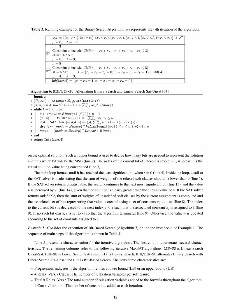
Table 3. Running example for the Binary Search Algorithm. #i represents the i-th iteration of the algorithm.


µ = 8, λ = −1;

#1

ν = 3Constraint to include: CNF(r1 + r2 + r3 + r4 + r5 + r6 + r7 ≤ 3)st = UNSAT;

µ = 8, λ = 3;

#2

ν = 5Constraint to include: CNF(r1 + r2 + r3 + r4 + r5 + r6 + r7 ≤ 5)st = SAT; A = {r3 = r5 = r7 = 0; r1 = r2 = r4 = r6 = 1} ∪ Init(A)µ = 4, λ = 3;

Init(lastA) = {x3 = x5 = 1;x1 = x2 = x4 = x6 = 0}

Algorithm 6: BIN/LIN-SU: Alternating Binary Search and Linear Search Sat-Unsat [64]

Input: ϕ

1 (R,ϕW )← RelaxCls(∅, ϕ, Cls(Soft(ϕ)))2 (λ, µ, lastA,mode)← (−1, 1 +

∑m

i=1wi, ∅, Binary)


4 ν ← (mode = Binary) ? ⌊µ+λ

2⌋ : µ− 1


i=1wi · ri ≤ ν))


i=1wi · (1−A〈ci \ {ri}〉))

7 else λ← (mode = Binary) ? RefineBound({wi | 1 ≤ i ≤ m}, ν)−1 : ν8 mode← (mode = Binary) ? Linear : Binary

9 end


on the optimal solution. Such an upper bound is used to decide how many bits are needed to represent the solution

and thus which bit will be the MSB (line 2). The index of the current bit of interest is stored in ι, whereas ν is the

actual solution value being constructed (line 3).

The main loop iterates until it has reached the least significant bit when ι = 0 (line 4). Inside the loop, a call to

the SAT solver is made stating that the sum of weights of the relaxed soft clauses should be lower than ν (line 5).

If the SAT solver returns unsatisfiable, the search continues to the next most significant bit (line 13), and the value

ν is increased by 2ι (line 14), given that the solution is clearly greater than the current value of ν. If the SAT solver

returns satisfiable, then the sum of weights of unsatisfied soft clauses by the current assignment is computed and

the associated set of bits representing that value is created using a set of constants s0, . . . , sk (line 8). The index

to the current bit ι is decreased to the next index j < ι such that the associated constant sj is assigned to 1 (line

9). If no such bit exists, ι is set to -1 so that the algorithm terminates (line 9). Otherwise, the value ν is updated

according to the set of constants assigned to 1.

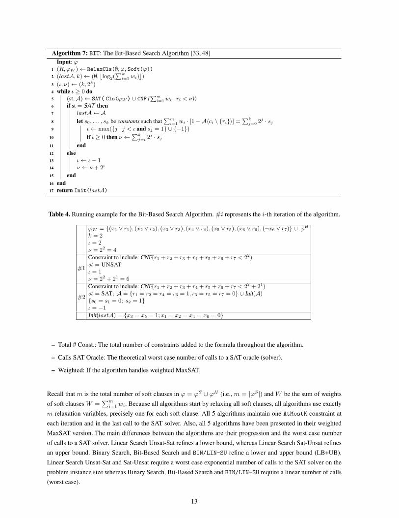
Example 5. Consider the execution of Bit-Based Search (Algorithm 7) on the the instance ϕ of Example 1. The

sequence of main steps of the algorithm is shown in Table 4.

Table 5 presents a characterization for the iterative algorithms. The first column enumerates several charac-

teristics. The remaining columns refer to the following iterative MaxSAT algorithms: LIN-US is Linear Search

Unsat-Sat, LIN-SU is Linear Search Sat-Unsat, BIN is Binary Search, BIN/LIN-SU alternates Binary Search with

Linear Search Sat-Unsat and BIT is Bit-Based Search. The considered characteristics are:

– Progression: indicates if the algorithm refines a lower bound (LB) or an upper bound (UB).

– # Relax. Vars. / Clause: The number of relaxation variables per soft clause.

– Total # Relax. Vars.: The total number of relaxation variables added to the formula throughout the algorithm.

– # Const. / Iteration: The number of constraints added at each iteration.

12

Algorithm 7: BIT: The Bit-Based Search Algorithm [33, 48]

Input: ϕ

1 (R,ϕW )← RelaxCls(∅, ϕ, Soft(ϕ))2 (lastA, k)← (∅, ⌊log2(

∑m

i=1wi)⌋)

3 (ι, ν)← (k, 2k)4 while ι ≥ 0 do

5 (st,A)← SAT( Cls(ϕW ) ∪ CNF (∑m

i=1wi · ri < ν))

6 if st = SAT then

7 lastA ← A

8 let s0, . . . , sk be constants such that∑m

i=1wi · [1−A〈ci \ {ri}〉] =

∑k

j=02j · sj

9 ι← max({j | j < ι and sj = 1} ∪ {−1})

10 if ι ≥ 0 then ν ←∑k

j=ι 2j · sj

11 end

12 else

13 ι← ι− 114 ν ← ν + 2ι

15 end

16 end


Table 4. Running example for the Bit-Based Search Algorithm. #i represents the i-th iteration of the algorithm.


k = 2ι = 2ν = 22 = 4

#1

Constraint to include: CNF(r1 + r2 + r3 + r4 + r5 + r6 + r7 < 22)st = UNSAT

ι = 1ν = 22 + 21 = 6

#2

Constraint to include: CNF(r1 + r2 + r3 + r4 + r5 + r6 + r7 < 22 + 21)st = SAT; A = {r1 = r2 = r4 = r6 = 1, r3 = r5 = r7 = 0} ∪ Init(A){s0 = s1 = 0; s2 = 1}ι = −1Init(lastA) = {x3 = x5 = 1;x1 = x2 = x4 = x6 = 0}

– Total # Const.: The total number of constraints added to the formula throughout the algorithm.

– Calls SAT Oracle: The theoretical worst case number of calls to a SAT oracle (solver).

– Weighted: If the algorithm handles weighted MaxSAT.

Recall that m is the total number of soft clauses in ϕ = ϕS ∪ ϕH (i.e., m = |ϕS |) and W be the sum of weights

of soft clauses W =∑m

i=1 wi. Because all algorithms start by relaxing all soft clauses, all algorithms use exactly

m relaxation variables, precisely one for each soft clause. All 5 algorithms maintain one AtMostK constraint at

each iteration and in the last call to the SAT solver. Also, all 5 algorithms have been presented in their weighted

MaxSAT version. The main differences between the algorithms are their progression and the worst case number

of calls to a SAT solver. Linear Search Unsat-Sat refines a lower bound, whereas Linear Search Sat-Unsat refines

an upper bound. Binary Search, Bit-Based Search and BIN/LIN-SU refine a lower and upper bound (LB+UB).

Linear Search Unsat-Sat and Sat-Unsat require a worst case exponential number of calls to the SAT solver on the

problem instance size whereas Binary Search, Bit-Based Search and BIN/LIN-SU require a linear number of calls

(worst case).

13

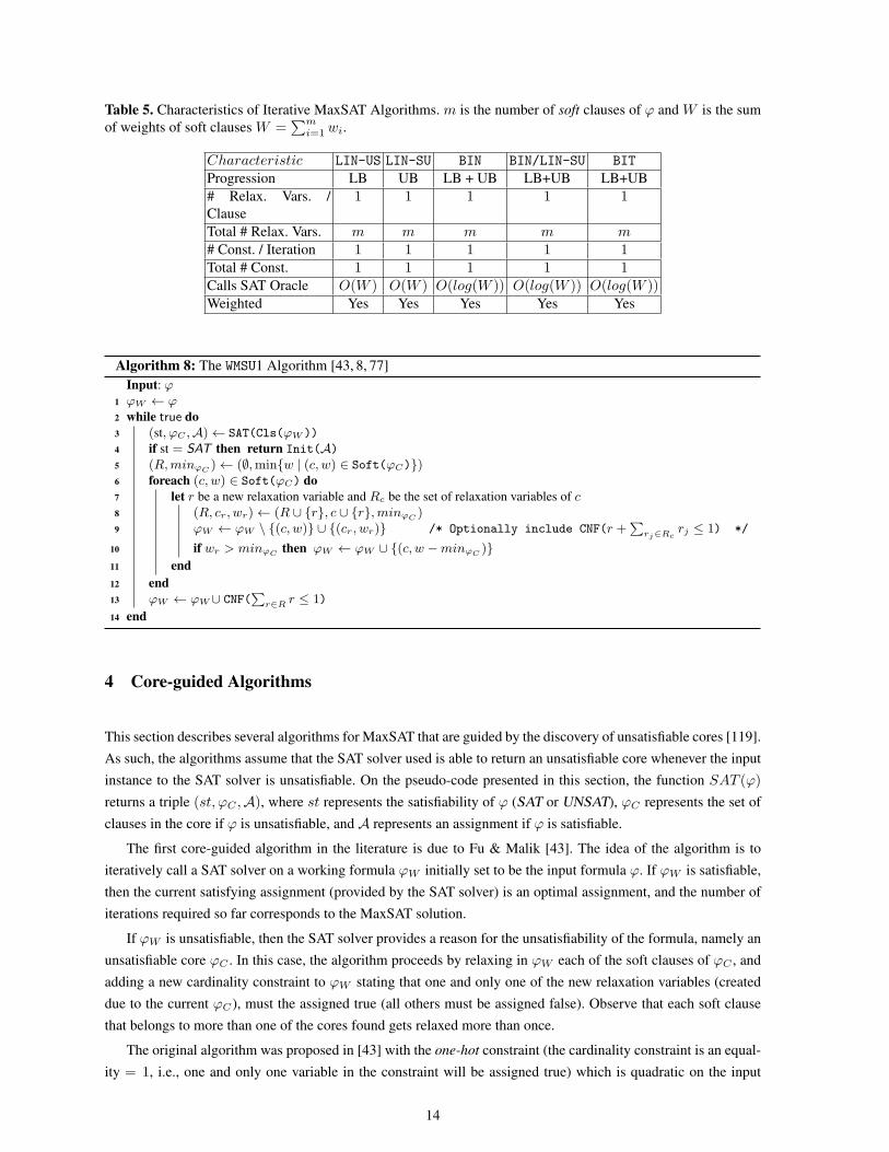
Table 5. Characteristics of Iterative MaxSAT Algorithms. m is the number of soft clauses of ϕ and W is the sum

of weights of soft clauses W =∑m

i=1 wi.

Characteristic LIN-US LIN-SU BIN BIN/LIN-SU BIT

Progression LB UB LB + UB LB+UB LB+UB

# Relax. Vars. /

Clause

1 1 1 1 1

Total # Relax. Vars. m m m m m

# Const. / Iteration 1 1 1 1 1Total # Const. 1 1 1 1 1Calls SAT Oracle O(W ) O(W ) O(log(W )) O(log(W )) O(log(W ))Weighted Yes Yes Yes Yes Yes

Algorithm 8: The WMSU1 Algorithm [43, 8, 77]

Input: ϕ

1 ϕW ← ϕ

2 while true do

3 (st, ϕC ,A)← SAT(Cls(ϕW ))

4 if st = SAT then return Init(A)5 (R,minϕC

)← (∅,min{w | (c, w) ∈ Soft(ϕC)})6 foreach (c, w) ∈ Soft(ϕC) do

7 let r be a new relaxation variable and Rc be the set of relaxation variables of c

8 (R, cr, wr)← (R ∪ {r}, c ∪ {r},minϕC)

9 ϕW ← ϕW \ {(c, w)} ∪ {(cr, wr)} /* Optionally include CNF(r +∑

rj∈Rcrj ≤ 1) */

10 if wr > minϕCthen ϕW ← ϕW ∪ {(c, w −minϕC

)}

11 end

12 end

13 ϕW ← ϕW∪ CNF(∑

r∈R r ≤ 1)

14 end

4 Core-guided Algorithms

This section describes several algorithms for MaxSAT that are guided by the discovery of unsatisfiable cores [119].

As such, the algorithms assume that the SAT solver used is able to return an unsatisfiable core whenever the input

instance to the SAT solver is unsatisfiable. On the pseudo-code presented in this section, the function SAT (ϕ)

returns a triple (st, ϕC ,A), where st represents the satisfiability of ϕ (SAT or UNSAT), ϕC represents the set of

clauses in the core if ϕ is unsatisfiable, and A represents an assignment if ϕ is satisfiable.

The first core-guided algorithm in the literature is due to Fu & Malik [43]. The idea of the algorithm is to

iteratively call a SAT solver on a working formula ϕW initially set to be the input formula ϕ. If ϕW is satisfiable,

then the current satisfying assignment (provided by the SAT solver) is an optimal assignment, and the number of

iterations required so far corresponds to the MaxSAT solution.

If ϕW is unsatisfiable, then the SAT solver provides a reason for the unsatisfiability of the formula, namely an

unsatisfiable core ϕC . In this case, the algorithm proceeds by relaxing in ϕW each of the soft clauses of ϕC , and

adding a new cardinality constraint to ϕW stating that one and only one of the new relaxation variables (created

due to the current ϕC), must the assigned true (all others must be assigned false). Observe that each soft clause

that belongs to more than one of the cores found gets relaxed more than once.

The original algorithm was proposed in [43] with the one-hot constraint (the cardinality constraint is an equal-

ity = 1, i.e., one and only one variable in the constraint will be assigned true) which is quadratic on the input

14

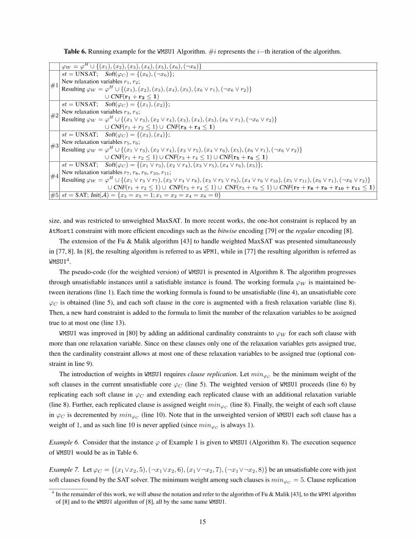
Table 6. Running example for the WMSU1 Algorithm. #i represents the i−th iteration of the algorithm.

ϕW = ϕH ∪ {(x1), (x2), (x3), (x4), (x5), (x6), (¬x6)}

#1

st = UNSAT; Soft(ϕC) = {(x6), (¬x6)};New relaxation variables r1, r2;

Resulting ϕW = ϕH ∪ {(x1), (x2), (x3), (x4), (x5), (x6 ∨ r1), (¬x6 ∨ r2)}∪ CNF(r1 + r2 ≤ 1)

#2

st = UNSAT; Soft(ϕC) = {(x1), (x2)};New relaxation variables r3, r4;

Resulting ϕW = ϕH ∪ {(x1 ∨ r3), (x2 ∨ r4), (x3), (x4), (x5), (x6 ∨ r1), (¬x6 ∨ r2)}∪ CNF(r1 + r2 ≤ 1) ∪ CNF(r3 + r4 ≤ 1)

#3

st = UNSAT; Soft(ϕC) = {(x3), (x4)};New relaxation variables r5, r6;

Resulting ϕW = ϕH ∪ {(x1 ∨ r3), (x2 ∨ r4), (x3 ∨ r5), (x4 ∨ r6), (x5), (x6 ∨ r1), (¬x6 ∨ r2)}∪ CNF(r1 + r2 ≤ 1) ∪ CNF(r3 + r4 ≤ 1) ∪ CNF(r5 + r6 ≤ 1)

#4

st = UNSAT; Soft(ϕC) = {(x1 ∨ r3), (x2 ∨ r4), (x3 ∨ r5), (x4 ∨ r6), (x5)};New relaxation variables r7, r8, r9, r10, r11;

Resulting ϕW = ϕH ∪ {(x1 ∨ r3 ∨ r7), (x2 ∨ r4 ∨ r8), (x3 ∨ r5 ∨ r9), (x4 ∨ r6 ∨ r10), (x5 ∨ r11), (x6 ∨ r1), (¬x6 ∨ r2)}∪ CNF(r1 + r2 ≤ 1) ∪ CNF(r3 + r4 ≤ 1) ∪ CNF(r5 + r6 ≤ 1) ∪ CNF(r7 + r8 + r9 + r10 + r11 ≤ 1)

#5 st = SAT; Init(A) = {x3 = x5 = 1;x1 = x2 = x4 = x6 = 0}

size, and was restricted to unweighted MaxSAT. In more recent works, the one-hot constraint is replaced by an

AtMost1 constraint with more efficient encodings such as the bitwise encoding [79] or the regular encoding [8].

The extension of the Fu & Malik algorithm [43] to handle weighted MaxSAT was presented simultaneously

in [77, 8]. In [8], the resulting algorithm is referred to as WPM1, while in [77] the resulting algorithm is referred as

WMSU14.

The pseudo-code (for the weighted version) of WMSU1 is presented in Algorithm 8. The algorithm progresses

through unsatisfiable instances until a satisfiable instance is found. The working formula ϕW is maintained be-

tween iterations (line 1). Each time the working formula is found to be unsatisfiable (line 4), an unsatisfiable core

ϕC is obtained (line 5), and each soft clause in the core is augmented with a fresh relaxation variable (line 8).

Then, a new hard constraint is added to the formula to limit the number of the relaxation variables to be assigned

true to at most one (line 13).

WMSU1 was improved in [80] by adding an additional cardinality constraints to ϕW for each soft clause with

more than one relaxation variable. Since on these clauses only one of the relaxation variables gets assigned true,

then the cardinality constraint allows at most one of these relaxation variables to be assigned true (optional con-

straint in line 9).

The introduction of weights in WMSU1 requires clause replication. Let minϕCbe the minimum weight of the

soft clauses in the current unsatisfiable core ϕC (line 5). The weighted version of WMSU1 proceeds (line 6) by

replicating each soft clause in ϕC and extending each replicated clause with an additional relaxation variable

(line 8). Further, each replicated clause is assigned weight minϕC(line 8). Finally, the weight of each soft clause

in ϕC is decremented by minϕC(line 10). Note that in the unweighted version of WMSU1 each soft clause has a

weight of 1, and as such line 10 is never applied (since minϕCis always 1).

Example 6. Consider that the instance ϕ of Example 1 is given to WMSU1 (Algorithm 8). The execution sequence

of WMSU1 would be as in Table 6.

Example 7. Let ϕC = {(x1∨x2, 5), (¬x1∨x2, 6), (x1∨¬x2, 7), (¬x1∨¬x2, 8)} be an unsatisfiable core with just

soft clauses found by the SAT solver. The minimum weight among such clauses is minϕC= 5. Clause replication

4 In the remainder of this work, we will abuse the notation and refer to the algorithm of Fu & Malik [43], to the WPM1 algorithm

of [8] and to the WMSU1 algorithm of [8], all by the same name WMSU1.

15

Algorithm 9: The MSU2 Algorithm [79]

Input: ϕ

1

2 function BinRelax (ϕI , ϕW )

3 (ϕo, k, n)← (∅, |ϕI |, 1)4 if k 6= 1 then n← ⌈log2 k⌉5 let r0, . . . , rn−1 be fresh relaxation variables

6 foreach i ∈ [0, k − 1] do

7 let ci is i-th clause of ϕI

8 foreach cR ∈ getAssocCls(ϕW , ci) do

9 foreach j ∈ [0, n− 1] do

10 if binary representation of i has value 1 in position j then ϕo ← ϕo ∪ {cR ∪ {rj}}11 else ϕo ← ϕo ∪ {cR ∪ {¬rj}}

12 end

13 end

14 end

15 end

16 end

17 return ϕo // Clauses in ϕo marked soft

18 end

19

20 ϕW ← ϕ

21 while true do

22 (st, ϕC ,A)← SAT(Cls(ϕW ))

23 if st = SAT or Soft(ϕC)= ∅ then return Init(A)24 (ϕI , ϕR)← (∅, ∅)25 foreach cR ∈ Soft(ϕC) do

26 c← getInitCl(ϕ, cR) /* getInitCl(ϕ, cR)= c ∈ ϕ such that cR = (c ∪⋃{r}) */

27 ϕI ← ϕI ∪ {c}28 ϕR ← ϕR ∪ getAssocCls(ϕW , c) /* getAssocCls(ϕW , c)= {cR | cR = (c ∪

⋃{r}) ∈ ϕW } */

29 end

30 ϕW ← ϕW \ ϕR ∪ BinRelax(ϕI , ϕW )

31 end

will create the following set of clauses with an additional relaxation variable: {(x1 ∨ x2 ∨ r1, 5), (¬x1 ∨ x2 ∨

r2, 5), (x1 ∨ ¬x2 ∨ r3, 5), (¬x1 ∨ ¬x2 ∨ r4, 5)} and the weight of the original soft clauses will be decremented

by minϕCresulting in {(¬x1 ∨ x2, 1), (x1 ∨ ¬x2, 2), (¬x1 ∨ ¬x2, 3)}.

Observe that WMSU1 is the only MaxSAT algorithm that adds more than one relaxation variable per soft clause.

Whereas the remaining MaxSAT algorithms described in this paper add and remove AtMostK constraints at each

iteration, WMSU1 is the only algorithm that just adds AtMost1 and AtLeast1 constraints that become part of the

working formula. For this reason, WMSU1 is said to transform each problem instance into an equivalent one at each

iteration in [8].

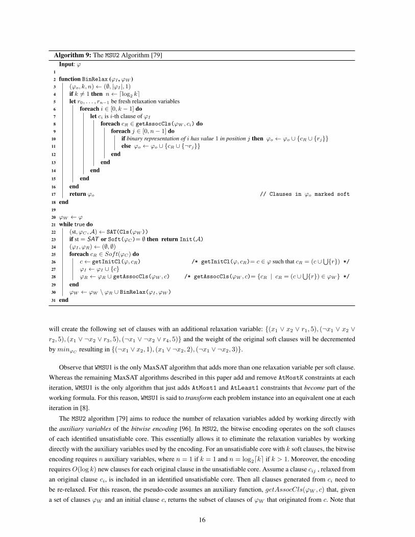
The MSU2 algorithm [79] aims to reduce the number of relaxation variables added by working directly with

the auxiliary variables of the bitwise encoding [96]. In MSU2, the bitwise encoding operates on the soft clauses

of each identified unsatisfiable core. This essentially allows it to eliminate the relaxation variables by working

directly with the auxiliary variables used by the encoding. For an unsatisfiable core with k soft clauses, the bitwise

encoding requires n auxiliary variables, where n = 1 if k = 1 and n = log2⌈k⌉ if k > 1. Moreover, the encoding

requiresO(log k) new clauses for each original clause in the unsatisfiable core. Assume a clause cij , relaxed from

an original clause ci, is included in an identified unsatisfiable core. Then all clauses generated from ci need to

be re-relaxed. For this reason, the pseudo-code assumes an auxiliary function, getAssocCls(ϕW , c) that, given

a set of clauses ϕW and an initial clause c, returns the subset of clauses of ϕW that originated from c. Note that

16

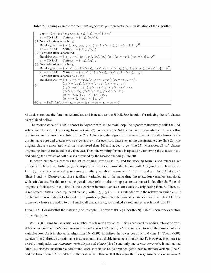
Table 7. Running example for the MSU2 Algorithm. #i represents the i−th iteration of the algorithm.

ϕW = {(x1), (x2), (x3), (x4), (x5), (x6), (¬x6)} ∪ ϕH

#1st = UNSAT; Soft(ϕC) = {(x6), (¬x6)};New relaxation variable r1;

Resulting ϕW = {(x1), (x2), (x3), (x4), (x5), (x6 ∨ ¬r1), (¬x6 ∨ r1)} ∪ ϕH

#2st = UNSAT; Soft(ϕC) = {(x1), (x2)};New relaxation variable r2;

Resulting ϕW = {(x1 ∨ ¬r2), (x2 ∨ r2), (x3), (x4), (x5), (x6 ∨ ¬r1), (¬x6 ∨ r1)} ∪ ϕH

#3st = UNSAT; Soft(ϕC) = {(x3), (x4)};New relaxation variable r3;

Resulting ϕW = {(x1 ∨ ¬r2), (x2 ∨ r2), (x3 ∨ ¬r3), (x4 ∨ r3), (x5), (x6 ∨ ¬r1), (¬x6 ∨ r1)} ∪ ϕH

#4

st = UNSAT; Soft(ϕC) = {(x1 ∨ r3), (x2 ∨ r4), (x3 ∨ r5), (x4 ∨ r6), (x5)};New relaxation variables r4, r5, r6;

Resulting ϕW = {(x1 ∨ ¬r2 ∨ ¬r4), (x1 ∨ ¬r2 ∨ ¬r5), (x1 ∨ ¬r2 ∨ ¬r6),(x2 ∨ r2 ∨ r4), (x2 ∨ r2 ∨ ¬r5), (x2 ∨ r2 ∨ ¬r6),(x3 ∨ ¬r3 ∨ ¬r4), (x3 ∨ ¬r3 ∨ r5), (x3 ∨ ¬r3 ∨ ¬r6),(x4 ∨ r3 ∨ r4), (x4 ∨ r3 ∨ r5), (x4 ∨ r3 ∨ ¬r6),(x5 ∨ ¬r4), (x5 ∨ ¬r5), (x5 ∨ r6),(x6 ∨ ¬r1), (¬x6 ∨ r1)} ∪ ϕH


MSU2 does not use the function RelaxCls, and instead uses the BinRelax function for relaxing the soft clauses

as explained bellow.

The pseudo-code of MSU2 is shown in Algorithm 9. In the main loop, the algorithm iteratively calls the SAT

solver with the current working formula (line 22). Whenever the SAT solver returns satisfiable, the algorithm

terminates and returns the solution (line 23). Otherwise, the algorithm traverses the set of soft clauses in the

unsatisfiable core and creates two sets ϕI and ϕR. For each soft clause cR in the unsatisfiable core (line 25), the

original clause c associated with cR is retrieved (line 26) and added to ϕI (line 27). Moreover, all soft clauses

originating from c are added to ϕR (line 28). Then, the working formula is updated by removing the clauses in ϕR

and adding the new set of soft clauses provided by the bitwise encoding (line 30).

Function BinRelax receives the set of original soft clauses ϕI and the working formula and returns a set

of new soft clauses ϕo. Initially, ϕo is empty (line 3). For an unsatisfiable core with k original soft clauses (i.e.,

k = |ϕI |), the bitwise encoding requires n auxiliary variables, where n = 1 if k = 1 and n = log2⌈k⌉ if k > 1

(lines 3 and 4). Observe that those auxiliary variables are at the same time the relaxation variables associated

with soft clauses. For this reason, the pseudo-code refers to them simply as relaxation variables (line 5). For each

original soft clause ci in ϕI (line 7), the algorithm iterates over each soft clause cR originating from ci. Then, cR

is replicated n times. Each replicated clause j with 0 ≤ j ≤ (n− 1) is extended with the relaxation variable rj if

the binary representation of i has value 1 in position j (line 10), otherwise it is extended with ¬rj (line 11). The

replicated clauses are added to ϕo. Finally, all clauses in ϕo are marked as soft and ϕo is returned (line 17).

Example 8. Consider that the instance ϕ of Example 1 is given to MSU2 (Algorithm 9). Table 7 shows the execution

of the algorithm.

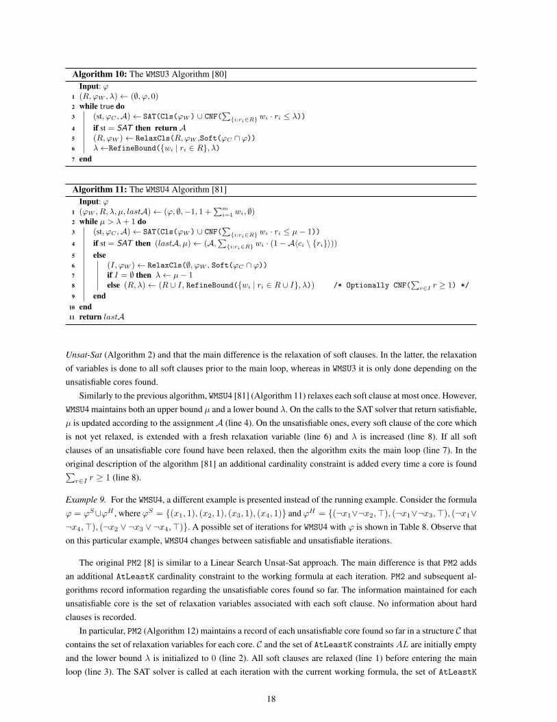
WMSU3 [80] aims to use a smaller number of relaxation variables. This is achieved by adding relaxation vari-

ables on demand and only one relaxation variable is added per soft clause, in order to keep the number of new

variables low. As it is shown in Algorithm 10, WMSU3 initializes the lower bound λ to 0 (line 1). Then, WMSU3

iterates (line 2) through unsatisfiable instances until a satisfiable instance is found (line 4). However, in contrast to

WMSU1, it only adds one relaxation variable per soft clause (line 5) and only one at most constraint is maintained

(line 3). For each unsatisfiable core found, each soft clause not yet relaxed gets a new relaxation variable (line 5)

and the lower bound λ is updated to the next value. Observe that this algorithm is very similar to Linear Search

17

Algorithm 10: The WMSU3 Algorithm [80]

Input: ϕ

1 (R,ϕW , λ)← (∅, ϕ, 0)2 while true do

3 (st, ϕC ,A)← SAT(Cls(ϕW ) ∪ CNF(∑

{i:ri∈R} wi · ri ≤ λ))

4 if st = SAT then return A5 (R,ϕW )← RelaxCls(R,ϕW ,Soft(ϕC ∩ ϕ))6 λ←RefineBound({wi | ri ∈ R}, λ)

7 end

Algorithm 11: The WMSU4 Algorithm [81]

Input: ϕ

1 (ϕW , R, λ, µ, lastA)← (ϕ, ∅,−1, 1 +∑m

i=1wi, ∅)

2 while µ > λ+ 1 do


{i:ri∈R} wi · ri ≤ µ− 1))

4 if st = SAT then (lastA, µ)← (A,∑

{i:ri∈R} wi · (1−A〈ci \ {ri}〉))

5 else

6 (I, ϕW )← RelaxCls(∅, ϕW , Soft(ϕC ∩ ϕ))7 if I = ∅ then λ← µ− 18 else (R, λ)← (R ∪ I, RefineBound({wi | ri ∈ R ∪ I}, λ)) /* Optionally CNF(

∑r∈I r ≥ 1) */

9 end

10 end

11 return lastA

Unsat-Sat (Algorithm 2) and that the main difference is the relaxation of soft clauses. In the latter, the relaxation

of variables is done to all soft clauses prior to the main loop, whereas in WMSU3 it is only done depending on the

unsatisfiable cores found.

Similarly to the previous algorithm, WMSU4 [81] (Algorithm 11) relaxes each soft clause at most once. However,

WMSU4 maintains both an upper bound µ and a lower bound λ. On the calls to the SAT solver that return satisfiable,

µ is updated according to the assignment A (line 4). On the unsatisfiable ones, every soft clause of the core which

is not yet relaxed, is extended with a fresh relaxation variable (line 6) and λ is increased (line 8). If all soft

clauses of an unsatisfiable core found have been relaxed, then the algorithm exits the main loop (line 7). In the

original description of the algorithm [81] an additional cardinality constraint is added every time a core is found∑

r∈I r ≥ 1 (line 8).

Example 9. For the WMSU4, a different example is presented instead of the running example. Consider the formula

ϕ = ϕS∪ϕH , where ϕS = {(x1, 1), (x2, 1), (x3, 1), (x4, 1)} and ϕH = {(¬x1∨¬x2,⊤), (¬x1∨¬x3,⊤), (¬x1∨

¬x4,⊤), (¬x2 ∨ ¬x3 ∨ ¬x4,⊤)}. A possible set of iterations for WMSU4 with ϕ is shown in Table 8. Observe that

on this particular example, WMSU4 changes between satisfiable and unsatisfiable iterations.

The original PM2 [8] is similar to a Linear Search Unsat-Sat approach. The main difference is that PM2 adds

an additional AtLeastK cardinality constraint to the working formula at each iteration. PM2 and subsequent al-

gorithms record information regarding the unsatisfiable cores found so far. The information maintained for each

unsatisfiable core is the set of relaxation variables associated with each soft clause. No information about hard

clauses is recorded.

In particular, PM2 (Algorithm 12) maintains a record of each unsatisfiable core found so far in a structure C that

contains the set of relaxation variables for each core. C and the set of AtLeastK constraintsAL are initially empty

and the lower bound λ is initialized to 0 (line 2). All soft clauses are relaxed (line 1) before entering the main

loop (line 3). The SAT solver is called at each iteration with the current working formula, the set of AtLeastK

18

Table 8. Running example for the WMSU4 Algorithm. #i represents the i−th iteration of the algorithm.

ϕW = {(x1), (x2), (x3), (x4)} ∪ ϕH

µ = 5; λ = −1;

#1st = UNSAT; Soft(ϕC) = {(x2), (x3), (x4)};λ = 0; New relaxation variables r1, r2, r3;

Resulting ϕW = {(x1), (x2 ∨ r1), (x3 ∨ r2), (x4 ∨ r3)} ∪ ϕH

#2Constraint to include: CNF(r1 + r2 + r3 ≤ 4)st = SAT; A = {x1 = r1 = r2 = r3 = 1;x2 = x3 = x4 = 0}µ = 3;

#3

Constraint to include: CNF(r1 + r2 + r3 ≤ 2)st = UNSAT; Soft(ϕC) = {(x1), (x2 ∨ r1), (x3 ∨ r2), (x4 ∨ r3)};λ = 1; New relaxation variable r4;

Resulting ϕW = {(x1 ∨ r4), (x2 ∨ r1), (x3 ∨ r2), (x4 ∨ r3)} ∪ ϕH

#4Constraint to include: CNF(r1 + r2 + r3 + r4 ≤ 2)st = SAT; A = {x1 = x2 = r3 = r4 = 0;x3 = x4 = r1 = r2 = 1}µ = 2;

Algorithm 12: The PM2 Algorithm [8]

Input: ϕ

1 (R,ϕW )← RelaxCls(∅, ϕ, Soft(ϕ))2 (λ, C, AL)← (0, ∅, ∅)3 while true do

4 (st, ϕC ,A)← SAT(Cls(ϕW ) ∪ CNF( AL ∪∑

r∈R r ≤ λ))5 if st = SAT or Soft(ϕC)= ∅ then return Init(A)6 RC ← {r | (c ∪ {r}) ∈ Soft(ϕC) and r ∈ R}7 C ← C ∪ {RC}8 k ← |{R ∈ C | R ⊆ RC}|9 AL← AL ∪

∑r∈RC

r ≥ k

10 λ← λ+ 1

11 end

constraints AL, and an AtMostK constraint bounded to the current lower bound λ (line 4). For each new core, the

relaxation variables associated with each soft clause are stored in RC (line 6), and the information of the new core

is added to the C structure (line 7). Then, the recorded cores C are traversed to check whether their soft clauses

are included in the new core. Finally, an AtLeastK cardinality constraint is added to the AL set (line 9), meaning

that the number of variables in the set of relaxation variables of the new core RC that need to be one is at least the

number of cores k included in such a new core, including itself (line 8). For the sake of clarity, the set of AtLeastK

constraints AL is maintained as an independent set but indeed each new AtLeastK constraint becomes part of the

working formula. However, the AtMostK constraint (line 4) is actually added and removed at each iteration.

PM2.1 [7] is an extension of PM2 that maintains sets of covers. Basically, each unsatisfiable core will result

in an AtLeastK cardinality constraint, and every cover in an AtMostK cardinality constraint. Let C be a set of

unsatisfiable cores. Each core R1 ∈ C is defined by the set of relaxation variables associated with the soft clauses.

A set of relaxation variables R2 is a cover of C if it is a minimal set such that, for each R1 ∈ C, if R1 ∩ R2 6= ∅,

then R1 ⊆ R2. The expression CoversOf(C) denotes the set of covers of C.

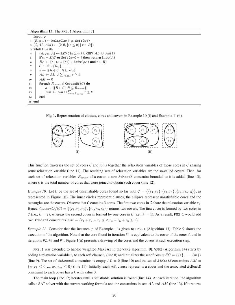
Algorithm 13 corresponds to PM2.1, and is similar to PM2 (lines 1 to 9). The main difference is that an addi-

tional set of AtMostK constraints AM is maintained which is initially empty (line 1). At each iteration, the SAT

solver is called with the current working formula and the sets AL and AM (line 3). Then, the set of AtLeastK

constraints AL is augmented in the same way as in PM2 (lines 6 to 9). Finally, the set of AtMostK constraints AM

is prepared for the next iteration. First, the set AM is emptied. Then, for each cover in C, AM is augmented with

an additional AtMostK constraint. Function CoversOf(C) divides the set of cores stored in C into a set of covers.

19

Algorithm 13: The PM2.1 Algorithm [7]

Input: ϕ

1 (R,ϕW )← RelaxCls(∅, ϕ, Soft(ϕ))2 (C, AL,AM)← (∅, ∅, {(r ≤ 0) | r ∈ R})3 while true do

4 (st, ϕC ,A)← SAT(Cls(ϕW ) ∪ CNF( AL ∪ AM))

5 if st = SAT or Soft(ϕC)= ∅ then return Init(A)6 RC ← {r | (c ∪ {r}) ∈ Soft(ϕC) and r ∈ R}7 C ← C ∪ {RC}8 k ← |{R ∈ C | R ⊆ RC}|9 AL← AL ∪

∑r∈RC

r ≥ k

10 AM ← ∅11 foreach Rcover ∈ CoversOf(C) do

12 k ← |{R ∈ C | R ⊆ Rcover}|13 AM ← AM ∪

∑r∈Rcover

r ≤ k

14 end

15 end

Fig. 1. Representation of clauses, cores and covers in Example 10 (i) and Example 11(ii).

r1 r2

r3

r4

r5

r6 r1 r2

r3 r4

r5 r6

r7

(i) (ii)

This function traverses the set of cores C and joins together the relaxation variables of those cores in C sharing

some relaxation variable (line 11). The resulting sets of relaxation variables are the so-called covers. Then, for

each set of relaxation variables Rcover of a cover, a new AtMostK constraint bounded to k is added (line 13),

where k is the total number of cores that were joined to obtain such cover (line 12).

Example 10. Let C be the set of unsatisfiable cores found so far with C = {{r1, r2}, {r1, r3}, {r4, r5, r6}}, as

represented in Figure 1(i). The inner circles represent clauses, the ellipses represent unsatisfiable cores and the

rectangles are the covers. Observe that C contains 3 cores. The first two cores in C share the relaxation variable r1.

Hence, CoversOf(C) = {{r1, r2, r3}, {r4, r5, r6}} returns two covers. The first cover is formed by two cores in

C (i.e., k = 2), whereas the second cover is formed by one core in C (i.e., k = 1). As a result, PM2.1 would add

two AtMostK constraints AM = {r1 + r2 + r3 ≤ 2, r4 + r5 + r6 ≤ 1}

Example 11. Consider that the instance ϕ of Example 1 is given to PM2.1 (Algorithm 13). Table 9 shows the

execution of the algorithm. Note that the core found in iteration #4 is equivalent to the cover of the cores found in

iterations #2, #3 and #4. Figure 1(ii) presents a drawing of the cores and the covers at such execution step.

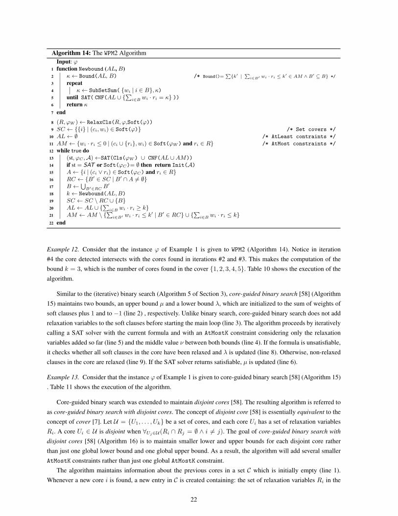
PM2.1 was extended to handle weighted MaxSAT in the WPM2 algorithm [9]. WPM2 (Algorithm 14) starts by

adding a relaxation variable ri to each soft clause ci (line 8) and initializes the set of covers SC = {{1}, . . . , {m}}

(line 9). The set of AtLeastK constraints is empty AL = ∅ (line 10) and the set of AtMostK constraints AM =

{w1r1 ≤ 0, ..., wmrm ≤ 0} (line 11). Initially, each soft clause represents a cover and the associated AtMostK

constraint to each cover has a k with value 0.

The main loop (line 12) iterates until a satisfiable solution is found (line 14). At each iteration, the algorithm

calls a SAT solver with the current working formula and the constraints in sets AL and AM (line 13). If it returns

20

Table 9. Running example for the PM2.1 Algorithm. #i represents the i−th iteration of the algorithm.


C = ∅ ; AL = ∅AM = (r1 ≤ 0), (r2 ≤ 0), (r3 ≤ 0), (r4 ≤ 0), (r5 ≤ 0), (r6 ≤ 0), (r7 ≤ 0)

#1

st = UNSAT; Soft(ϕC) = {(x6 ∨ r6), (¬x6 ∨ r7)}RC = {r6, r7}C = {{r6, r7}}k = 1AL = {(r6 + r7 ≥ 1)}AM = {(r1 ≤ 0), (r2 ≤ 0), (r3 ≤ 0), (r4 ≤ 0), (r5 ≤ 0), (r6 + r7 ≤ 1)}

#2

st = UNSAT; Soft(ϕC) = {(x1 ∨ r1), (x2 ∨ r2)}RC = {r1, r2}C = {{r6, r7}, {r1, r2}}k = 1AL = {(r6 + r7 ≥ 1), (r1 + r2 ≥ 1)}AM = {(r3 ≤ 0), (r4 ≤ 0), (r5 ≤ 0), (r6 + r7 ≤ 1), (r1 + r2 ≤ 1)}

#3

st = UNSAT; Soft(ϕC) = {(x3 ∨ r3), (x4 ∨ r4)}RC = {r3, r4}C = {{r1, r2}, {r6, r7}, {r3, r4}}k = 1AL = {(r1 + r2 ≥ 1), (r6 + r7 ≥ 1), (r3 + r4 ≥ 1)}AM = {(r1 + r2 ≤ 1), (r5 ≤ 0), (r6 + r7 ≤ 1), (r3 + r4 ≤ 1)}

#4

st = UNSAT; Soft(ϕC) = {(x1 ∨ r1), (x2 ∨ r2), (x3 ∨ r3), (x4 ∨ r4), (x5 ∨ r5)}RC = {r1, r2, r3, r4, r5}C = {{r1, r2}, {r3, r4}, {r6, r7}, {r1, r2, r3, r4, r5}}k = 3AL = {(r1 + r2 ≥ 1), (r3 + r4 ≥ 1), (r6 + r7 ≥ 1), (r1 + r2 + r3 + r4 + r5 ≥ 1)}AM = {(r6 + r7 ≤ 1), (r1 + r2 + r3 + r4 + r5 ≤ 3)}


unsatisfiable, then the information of the unsatisfiable core obtained by the SAT solver is used to update the sets

SC, AL, and AM . Observe that there is one AtMostK constraint for each cover at each iteration, whereas one

AtLeastK constraint for each cover is added to the working formula at each iteration. One contribution of WPM2 is

the way it computes the bound k associated with each AtMostK and AtLeastK constraints, which is stronger for

weighted MaxSAT than just using the subset sum approach. First, the algorithm computes the set of all indexes A

of the relaxation variables associated with soft clauses in the unsatisfiable core (line 15). Then, the set of covers

in SC that share some variable with A are stored in RC (line 16). The covers in RC should be merged in just

one cover. The indexes of the relaxation variables contained in RC are stored in B (line 17). At this point, the

algorithm proceeds by computing the value k for the new cover defined over the relaxation variables in B. This is

done in function Newbound (line 18).

An initial bound k is computed that is essentially the sum of all k of the previous covers contained in the new

one (line 2). Then, the function iteratively refines the value of k until a valid value is obtained given the set of

weights. The subset sum is computed with the set of weights of the soft clauses referenced by the indexes in B

and the current k (line 4). Then, the SAT solver is called with the set of AtLeastK constraints AL and an equality

constraint that states that the weights inB should be equal to k (line 5). The algorithm iterates until the SAT solver

returns satisfiable.

WPM2 continues by removing the set of covers in RC from SC and replacing them with the new unique cover

defined in B (line 19). Then, the set of AtLeastK constraints AL is augmented with an additional AtLeastK

constraint bounded by the variables in B and the obtained k (line 20). Finally, the set of AtMostK constraints

related to the covers in RC are removed from AM and a new AtMostK constraint is added again bounded by the

variables in B and the obtained k (line 21).

21

Algorithm 14: The WPM2 Algorithm

Input: ϕ

1 function Newbound (AL, B)

2 κ← Bound(AL, B) /* Bound()=∑

{k′ |∑

i∈B′ wi · ri ≤ k′ ∈ AM ∧ B′ ⊆ B} */

3 repeat

4 κ← SubSetSum( {wi | i ∈ B}, κ)5 until SAT( CNF(AL ∪ {

∑i∈B wi · ri = κ} ))

6 return κ

7 end

8 (R,ϕW )← RelaxCls(R,ϕ,Soft(ϕ))

9 SC ← {{i} | (ci, wi) ∈ Soft(ϕ)} /* Set covers */

10 AL← ∅ /* AtLeast contraints */

11 AM ← {wi · ri ≤ 0 | (ci ∪ {ri}, wi) ∈ Soft(ϕW ) and ri ∈ R} /* AtMost constraints */

12 while true do

13 (st, ϕC ,A)←SAT(Cls(ϕW ) ∪ CNF(AL ∪AM))

14 if st = SAT or Soft(ϕC)= ∅ then return Init(A)15 A← {i | (ci ∨ ri) ∈ Soft(ϕC) and ri ∈ R}16 RC ← {B′ ∈ SC | B′ ∩A 6= ∅}17 B ←

⋃B′∈RC B

′

18 k ← Newbound(AL,B)

19 SC ← SC \RC ∪ {B}20 AL← AL ∪ {

∑i∈B wi · ri ≥ k}

21 AM ← AM \ {∑

i∈B′ wi · ri ≤ k′ | B′ ∈ RC} ∪ {

∑i∈B wi · ri ≤ k}

22 end

Example 12. Consider that the instance ϕ of Example 1 is given to WPM2 (Algorithm 14). Notice in iteration

#4 the core detected intersects with the cores found in iterations #2 and #3. This makes the computation of the

bound k = 3, which is the number of cores found in the cover {1, 2, 3, 4, 5}. Table 10 shows the execution of the

algorithm.

Similar to the (iterative) binary search (Algorithm 5 of Section 3), core-guided binary search [58] (Algorithm

15) maintains two bounds, an upper bound µ and a lower bound λ, which are initialized to the sum of weights of

soft clauses plus 1 and to −1 (line 2) , respectively. Unlike binary search, core-guided binary search does not add

relaxation variables to the soft clauses before starting the main loop (line 3). The algorithm proceeds by iteratively

calling a SAT solver with the current formula and with an AtMostK constraint considering only the relaxation

variables added so far (line 5) and the middle value ν between both bounds (line 4). If the formula is unsatisfiable,

it checks whether all soft clauses in the core have been relaxed and λ is updated (line 8). Otherwise, non-relaxed

clauses in the core are relaxed (line 9). If the SAT solver returns satisfiable, µ is updated (line 6).

Example 13. Consider that the instance ϕ of Example 1 is given to core-guided binary search [58] (Algorithm 15)

. Table 11 shows the execution of the algorithm.

Core-guided binary search was extended to maintain disjoint cores [58]. The resulting algorithm is referred to

as core-guided binary search with disjoint cores. The concept of disjoint core [58] is essentially equivalent to the

concept of cover [7]. Let U = {U1, . . . , Uk} be a set of cores, and each core Ui has a set of relaxation variables

Ri. A core Ui ∈ U is disjoint when ∀Uj∈U (Ri ∩ Rj = ∅ ∧ i 6= j). The goal of core-guided binary search with

disjoint cores [58] (Algorithm 16) is to maintain smaller lower and upper bounds for each disjoint core rather

than just one global lower bound and one global upper bound. As a result, the algorithm will add several smaller

AtMostK constraints rather than just one global AtMostK constraint.

The algorithm maintains information about the previous cores in a set C which is initially empty (line 1).

Whenever a new core i is found, a new entry in C is created containing: the set of relaxation variables Ri in the

22

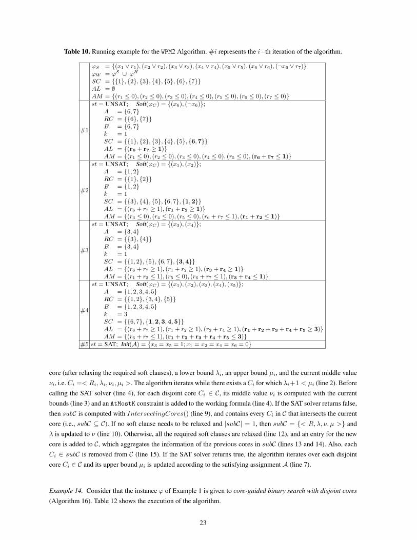
Table 10. Running example for the WPM2 Algorithm. #i represents the i−th iteration of the algorithm.

ϕS = {(x1 ∨ r1), (x2 ∨ r2), (x3 ∨ r3), (x4 ∨ r4), (x5 ∨ r5), (x6 ∨ r6), (¬x6 ∨ r7)}ϕW = ϕS ∪ ϕH

SC = {{1}, {2}, {3}, {4}, {5}, {6}, {7}}AL = ∅AM = {(r1 ≤ 0), (r2 ≤ 0), (r3 ≤ 0), (r4 ≤ 0), (r5 ≤ 0), (r6 ≤ 0), (r7 ≤ 0)}

#1

st = UNSAT; Soft(ϕC) = {(x6), (¬x6)};A = {6, 7}RC = {{6}, {7}}B = {6, 7}k = 1SC = {{1}, {2}, {3}, {4}, {5}, {6,7}}AL = {(r6 + r7 ≥ 1)}AM = {(r1 ≤ 0), (r2 ≤ 0), (r3 ≤ 0), (r4 ≤ 0), (r5 ≤ 0), (r6 + r7 ≤ 1)}

#2

st = UNSAT; Soft(ϕC) = {(x1), (x2)};A = {1, 2}RC = {{1}, {2}}B = {1, 2}k = 1SC = {{3}, {4}, {5}, {6, 7}, {1,2}}AL = {(r6 + r7 ≥ 1), (r1 + r2 ≥ 1)}AM = {(r3 ≤ 0), (r4 ≤ 0), (r5 ≤ 0), (r6 + r7 ≤ 1), (r1 + r2 ≤ 1)}

#3

st = UNSAT; Soft(ϕC) = {(x3), (x4)};A = {3, 4}RC = {{3}, {4}}B = {3, 4}k = 1SC = {{1, 2}, {5}, {6, 7}, {3,4}}AL = {(r6 + r7 ≥ 1), (r1 + r2 ≥ 1), (r3 + r4 ≥ 1)}AM = {(r1 + r2 ≤ 1), (r5 ≤ 0), (r6 + r7 ≤ 1), (r3 + r4 ≤ 1)}

#4

st = UNSAT; Soft(ϕC) = {(x1), (x2), (x3), (x4), (x5)};A = {1, 2, 3, 4, 5}RC = {{1, 2}, {3, 4}, {5}}B = {1, 2, 3, 4, 5}k = 3SC = {{6, 7}, {1,2,3,4,5}}AL = {(r6 + r7 ≥ 1), (r1 + r2 ≥ 1), (r3 + r4 ≥ 1), (r1 + r2 + r3 + r4 + r5 ≥ 3)}AM = {(r6 + r7 ≤ 1), (r1 + r2 + r3 + r4 + r5 ≤ 3)}


core (after relaxing the required soft clauses), a lower bound λi, an upper bound µi, and the current middle value

νi, i.e.Ci =< Ri, λi, νi, µi >. The algorithm iterates while there exists aCi for which λi+1 < µi (line 2). Before

calling the SAT solver (line 4), for each disjoint core Ci ∈ C, its middle value νi is computed with the current

bounds (line 3) and an AtMostK constraint is added to the working formula (line 4). If the SAT solver returns false,

then subC is computed with IntersectingCores() (line 9), and contains every Ci in C that intersects the current

core (i.e., subC ⊆ C). If no soft clause needs to be relaxed and |subC| = 1, then subC = {< R, λ, ν, µ >} and

λ is updated to ν (line 10). Otherwise, all the required soft clauses are relaxed (line 12), and an entry for the new

core is added to C, which aggregates the information of the previous cores in subC (lines 13 and 14). Also, each

Ci ∈ subC is removed from C (line 15). If the SAT solver returns true, the algorithm iterates over each disjoint

core Ci ∈ C and its upper bound µi is updated according to the satisfying assignment A (line 7).

Example 14. Consider that the instance ϕ of Example 1 is given to core-guided binary search with disjoint cores

(Algorithm 16). Table 12 shows the execution of the algorithm.

23

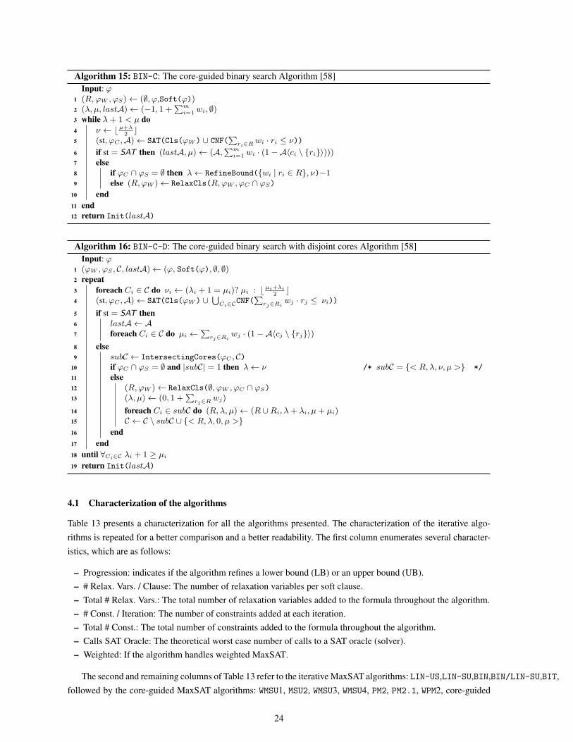
Algorithm 15: BIN-C: The core-guided binary search Algorithm [58]

Input: ϕ

1 (R,ϕW , ϕS)← (∅, ϕ,Soft(ϕ))2 (λ, µ, lastA)← (−1, 1 +

∑m

i=1wi, ∅)


4 ν ← ⌊µ+λ

2⌋


ri∈R wi · ri ≤ ν))


i=1wi · (1−A〈ci \ {ri}〉)))

7 else

8 if ϕC ∩ ϕS = ∅ then λ← RefineBound({wi | ri ∈ R}, ν)−19 else (R,ϕW )← RelaxCls(R,ϕW , ϕC ∩ ϕS)

10 end

11 end


Algorithm 16: BIN-C-D: The core-guided binary search with disjoint cores Algorithm [58]

Input: ϕ

1 (ϕW , ϕS , C, lastA)← (ϕ, Soft(ϕ), ∅, ∅)2 repeat

3 foreach Ci ∈ C do νi ← (λi + 1 = µi)? µi : ⌊µi+λi

2⌋

4 (st, ϕC ,A)← SAT(Cls(ϕW ) ∪⋃

Ci∈CCNF(∑

rj∈Riwj · rj ≤ νi))

5 if st = SAT then

6 lastA ← A7 foreach Ci ∈ C do µi ←

∑rj∈Ri

wj · (1−A〈cj \ {rj}〉)

8 else

9 subC ← IntersectingCores(ϕC , C)10 if ϕC ∩ ϕS = ∅ and |subC| = 1 then λ← ν /* subC = {< R, λ, ν, µ >} */

11 else

12 (R,ϕW )← RelaxCls(∅, ϕW , ϕC ∩ ϕS)

13 (λ, µ)← (0, 1 +∑

rj∈R wj)

14 foreach Ci ∈ subC do (R, λ, µ)← (R ∪Ri, λ+ λi, µ+ µi)15 C ← C \ subC ∪ {< R, λ, 0, µ >}

16 end

17 end

18 until ∀Ci∈C λi + 1 ≥ µi


4.1 Characterization of the algorithms

Table 13 presents a characterization for all the algorithms presented. The characterization of the iterative algo-

rithms is repeated for a better comparison and a better readability. The first column enumerates several character-

istics, which are as follows:

– Progression: indicates if the algorithm refines a lower bound (LB) or an upper bound (UB).

– # Relax. Vars. / Clause: The number of relaxation variables per soft clause.

– Total # Relax. Vars.: The total number of relaxation variables added to the formula throughout the algorithm.

– # Const. / Iteration: The number of constraints added at each iteration.

– Total # Const.: The total number of constraints added to the formula throughout the algorithm.

– Calls SAT Oracle: The theoretical worst case number of calls to a SAT oracle (solver).

– Weighted: If the algorithm handles weighted MaxSAT.

The second and remaining columns of Table 13 refer to the iterative MaxSAT algorithms: LIN-US,LIN-SU,BIN,BIN/LIN-SU,BIT,

followed by the core-guided MaxSAT algorithms: WMSU1, MSU2, WMSU3, WMSU4, PM2, PM2.1, WPM2, core-guided

24

Table 11. Running example for the core-guided binary search Algorithm. #i represents the i−th iteration of the

algorithm.

R = ∅; ϕW = ϕ; ϕS = {(x1), (x2), (x3), (x4), (x5), (x6), (¬x6)};µ = 8; λ = −1; lastA = ∅;

#1

ν = 3; Constraint to include: CNF(∅) = ∅;st = UNSAT; Soft(ϕC) = {(x6), (¬x6)};R = {r1, r2};ϕW = {(x6 ∨ r1), (¬x6 ∨ r2), (x1), (x2), (x3), (x4), (x5)} ∪ ϕ

H ;

#2

ν = 3; Constraint to include: CNF(r1 + r2 ≤ 3);st = UNSAT; Soft(ϕC) = {(x1), (x2)};R = {r1, r2, r3, r4};ϕW = {(x6 ∨ r1), (¬x6 ∨ r2), (x1 ∨ r3), (x2 ∨ r4), (x3), (x4), (x5)} ∪ ϕ

H ;

#3

ν = 3; Constraint to include: CNF(r1 + r2 + r3 + r4 ≤ 3);st = UNSAT; Soft(ϕC) = {(x3), (x4)};R = {r1, r2, r3, r4, r5, r6};ϕW = {(x6 ∨ r1), (¬x6 ∨ r2), (x1 ∨ r3), (x2 ∨ r4), (x3 ∨ r5), (x4 ∨ r6), (x5)} ∪ ϕ

H ;

#4

ν = 3; Constraint to include: CNF(r1 + r2 + r3 + r4 + r5 + r6 ≤ 3);st = UNSAT; Soft(ϕC) = {(x6 ∨ r1), (¬x6 ∨ r2), (x1 ∨ r3), (x2 ∨ r4), (x3 ∨ r5), (x4 ∨ r6), (x5)};R = {r1, r2, r3, r4, r5, r6, r7};ϕW = {(x6 ∨ r1), (¬x6 ∨ r2), (x1 ∨ r3), (x2 ∨ r4), (x3 ∨ r5), (x4 ∨ r6), (x5 ∨ r7)} ∪ ϕ

H ;

#5ν = 3; Constraint to include: CNF(r1 + r2 + r3 + r4 + r5 + r6 + r7 ≤ 3);st = UNSAT; Soft(ϕC) = {(x6 ∨ r1), (¬x6 ∨ r2), (x1 ∨ r3), (x2 ∨ r4), (x3 ∨ r5), (x4 ∨ r6), (x5 ∨ r7)};λ = 3;

#6ν = 5; Constraint to include: CNF(r1 + r2 + r3 + r4 + r5 + r6 + r7 ≤ 5);st = SAT; lastA = A = {r2 = r5 = r7 = 0; r1 = r3 = r4 = r6 = 1} ∪ Init(A);µ = 4;

Init(lastA) = {x3 = x5 = 1;x1 = x2 = x4 = x6 = 0}

binary search as BIN-C and core-guided binary search with disjoint cores as BIN-C-D. For an explanation on the

iterative MaxSAT algorithms, we refer to Table 5 on 14.

Recall thatm is the total number of soft clauses in ϕ = ϕS∪ϕH (i.e.,m = |ϕS |) andW be the sum of weights

of soft clauses W =∑m

i=1 wi. First, observe that except MSU2, PM2, and PM2.1, the algorithms are presented in

their weighted MaxSAT version. WMSU1, MSU2, WMSU3, PM2, PM2.1 and WPM2 all refine a lower bound. Differently,

WMSU4 alternates the refinement of a lower bound and an upper bound. Core-guided binary search and core-guided

binary search with disjoint cores both compute the middle value between the lower bound and upper bound.

PM2, PM2.1, and WPM2 add exactly one relaxation variable per soft clause and exactly a total of m relaxation

variables. WMSU3, WMSU4, core-guided binary search and core-guided binary search with disjoint cores relax vari-

ables on demand, so they may add one relaxation variable or none to each soft clause and a total of m in the worst

case (i.e., all soft clauses are relaxed). MSU2 requires log(m) relaxation variables per soft clause and a total of

O(m log(m)) relaxation variables throughout the algorithm. WMSU1 is the only algorithm that adds more than one

relaxation variable per soft clause. In the worst case, each soft clause can be relaxed W times. The total number

of relaxation variables γ for WMSU1 is detailed in the appendix.

WMSU1 adds one AtMost1 constraint at each iteration and a total of W in the worse case. MSU2 has no con-

straints; it just adds relaxation variables. WMSU3, WMSU4, PM2, and BIN-C add (and remove) one AtMostK constraint

at each iteration. PM2.1, WPM2, and BIN-C-D add (and remove) at most m AtMostK constraints at each iteration,

exactly one for each cover / disjoint core. Additionally, PM2, PM2.1, and WPM2 add one AtLeastK constraint at

each iteration. All of the algorithms require an exponential number of calls to the SAT solver, except BIN-C and

BIN-C-D which require a linear number of calls.

25

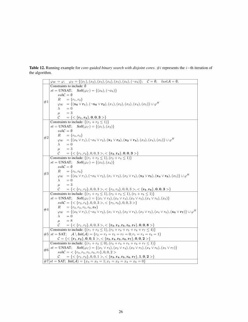
Table 12. Running example for core-guided binary search with disjoint cores. #i represents the i−th iteration of

the algorithm.

ϕW = ϕ; ϕS = {(x1), (x2), (x3), (x4), (x5), (x6), (¬x6)}; C = ∅; lastA = ∅;

#1

Constraints to include: ∅st = UNSAT; Soft(ϕC) = {(x6), (¬x6)}

subC = ∅R = {r1, r2}ϕW = {(x6 ∨ r1), (¬x6 ∨ r2), (x1), (x2), (x3), (x4), (x5)} ∪ ϕ

H

λ = 0µ = 3C = {< {r1, r2},0,0,3 >}

#2

Constraints to include: {(r1 + r2 ≤ 1)}st = UNSAT; Soft(ϕC) = {(x1), (x2)}

subC = ∅R = {r3, r4}ϕW = {(x6 ∨ r1), (¬x6 ∨ r2), (x1 ∨ r3), (x2 ∨ r4), (x3), (x4), (x5)} ∪ ϕ

H

λ = 0µ = 3C = {< {r1, r2}, 0, 0, 3 >,< {r3, r4},0,0,3 >}

#3

Constraints to include: {(r1 + r2 ≤ 1), (r3 + r4 ≤ 1)}st = UNSAT; Soft(ϕC) = {(x3), (x4)}

subC = ∅R = {r5, r6}ϕW = {(x6 ∨ r1), (¬x6 ∨ r2), (x1 ∨ r3), (x2 ∨ r4), (x3 ∨ r5), (x4 ∨ r6), (x5)} ∪ ϕ

H

λ = 0µ = 3C = {< {r1, r2}, 0, 0, 3 >,< {r3, r4}, 0, 0, 3 >,< {r5, r6},0,0,3 >}

#4

Constraints to include: {(r1 + r2 ≤ 1), (r3 + r4 ≤ 1), (r5 + r6 ≤ 1)}st = UNSAT; Soft(ϕC) = {(x1 ∨ r3), (x2 ∨ r4), (x3 ∨ r5), (x4 ∨ r6), (x5)}

subC = {< {r3, r4}, 0, 0, 3 >,< {r5, r6}, 0, 0, 3 >}R = {r3, r4, r5, r6, r7}ϕW = {(x6 ∨ r1), (¬x6 ∨ r2), (x1 ∨ r3), (x2 ∨ r4), (x3 ∨ r5), (x4 ∨ r6), (x5 ∨ r7)} ∪ ϕ

H

λ = 0µ = 8C = {< {r1, r2}, 0, 0, 3 >,< {r3, r4, r5, r6, r7},0,0,8 >}

#5Constraints to include: {(r1 + r2 ≤ 1), (r3 + r4 + r5 + r6 + r7 ≤ 4)}st = SAT; A \ Init(A) = {r2 = r3 = r5 = r7 = 0; r1 = r4 = r6 = 1}C = {< {r1, r2},0,0,1 >,< {r3, r4, r5, r6, r7},0,0,2 >}

#6

Constraints to include: {(r1 + r2 ≤ 0), (r3 + r4 + r5 + r6 + r7 ≤ 1)}st = UNSAT; Soft(ϕC) = {(x1 ∨ r3), (x2 ∨ r4), (x3 ∨ r5), (x4 ∨ r6), (x5 ∨ r7)}

subC = < {r3, r4, r5, r6, r7}, 0, 0, 2 >C = {< {r1, r2}, 0, 0, 1 >,< {r3, r4, r5, r6, r7},1,0,2 >}


26

Table 13. Characteristics of iterative and core-guided MaxSAT Algorithms. m is the number of soft clauses of ϕ and W is the sum of weights of soft clauses W =∑m

i=1 wi.

Charact. LIN-US LIN-SU BIN BIN/LIN-SU BIT WMSU1 MSU2 WMSU3 WMSU4 PM2 PM2.1 WPM2 BIN-C BIN-C-D

Progression LB UB LB + UB LB+UB LB+UB LB LB LB LB + UB LB LB LB LB + UB LB + UB

# Relax.

Vars. /

Clause

1 1 1 1 1 O(W ) O(log(m)) 1 or 0 1 or 0 1 1 1 1 or 0 1 or 0

Total # Re-

lax. Vars.

m m m m m γ O(m log(m)) O(m) O(m) m m m O(m) O(m)

# Const. / It-

eration

1 1 1 1 1 1 0 1 1 1 + 1 1 +O(m) 1 +O(m) 1 O(m)

Total #

Const.

1 1 1 1 1 O(W ) 0 1 1 1 +O(m) O(m) +O(m) O(W ) +O(m) 1 O(m)

Calls SAT

Oracle

O(W ) O(W ) O(log(W )) O(log(W )) O(log(W )) O(W ) O(m) O(W ) O(W ) O(m) O(m) O(W ) m+O(log(W )) m+O(log(W ))

Weighted Yes Yes Yes Yes Yes Yes No Yes Yes No No Yes Yes Yes

27

5 MaxSMT: A MaxSAT generalization for SMT

The Satisfiability Modulo Theories problem, or SMT, is an extension of Boolean Satisfiability where the goal is

to check the satisfiability of an SMT formula with respect to a background theory T [90, 104, 20]. As such, an

SMT formula is allowed to have atomic formulas or predicates in higher-level theories, such as linear arithmetic

or a higher-order logic, in addition to Boolean variables and their negations. As an example, the following SMT

formula mixes Boolean literals and linear inequalities: (a ∨ (5x− y ≤ 3)) ∧ (¬a ∨ (x+ y ≤ 12)).

Algorithms for solving SMT problems often have a core engine that is similar to a modern SAT solver. The

core engine then employs additional theory solvers that can process conjunctions of literals over the given theories

(every SMT solver handles some subset of possible theories). Further details on SMT, theories, and SMT solving

can be obtained in [90, 104].

The MaxSMT problem is a generalization of MaxSAT to the SMT domain. Given an SMT formula ϕ, MaxSMT

is the problem of finding a model A, consistent with the theories in ϕ, that maximizes the number of satisfied

clauses in ϕ. As in SAT, weights can be given to every clause in a SMT formula, and Weighted Partial MaxSMT

follows directly from its SAT equivalent.

Given the similarities between SAT and SMT, many algorithms for MaxSAT can be adapted to the MaxSMT

problem, and existing MaxSMT algorithms closely resemble the MaxSAT algorithms presented in this survey.

The first work to address MaxSMT can be found in [89]. In this work, SMT is extended to allow theories to be

strengthened, essentially letting the context in which a formula is evaluated change without altering the formula

itself. Then, an approach is proposed using their framework to solve weighted MaxSMT by placing information

about an objective function, and a bound on it, in the theory solver itself. In this approach, initially every weighted

clause (ci, wi) receives a new Boolean variable pi, and the constraints (pi → (ki = wi)), and (¬pi → (ki = 0))

are added to the theory. Further, the constraint (k1 + . . . + km ≤ B) is added to the theory together with the

relation (B < B0) (where B0 is an estimation of the initial cost). Each time a new cost Bi is found, the theory is

strengthened by adding the relation (B < Bi) to the theory. In this way, progressively better solutions are found,

minimizing the total cost of unsatisfied clauses by making the theory solver reject models worse than the best

known thus far. The final model found will be a MaxSMT solution. Of the MaxSAT algorithms presented earlier,

this algorithm is similar to the Linear Search Sat-Unsat algorithm; both explore a solution space of models that

satisfy some subset of clauses, requiring ever lower costs for those clauses not satisfied by the models, until no

further models can be found. The related Linear Search Unsat-Sat algorithm could not be applied in this extended

SMT framework directly, as it requires relaxing the constraint that bounds the cost of unsatisfied clauses in each

iteration, and the framework only allows theories to be strengthened.

The work in [32] proposed a “theory of Costs” C, along with a decision procedure for it, that allows modeling

multiple cost functions within the SMT framework. In [32], the theory of costs C is used to address the problem

of minimizing the value of one cost function subject to the satisfaction of an SMT formula named as the Boolean

Optimization Modulo Theory (BOMT) problem. The optimization itself can be performed by asserting atoms of C

that bound one cost function and using an incremental SMT solver.

Essentially, [32] proposed to encode the weighted partial MaxSMT problem into BOMT by adding a new

Boolean variable Aij to each soft clause. Then, the cost function is the sum of the weights of the soft clauses

whose variable Aij is assigned true. Again, this is similar to existing MaxSAT approaches that use relaxation

variables, and so an algorithm similar to Linear Search Sat-Unsat is described in such paper as well as a Binary

Search. While this is similar to the early work in [89], it differs in that it allows for multiple cost functions and in

that it does not require strengthening the theory to update cost bounds.

While both of the above techniques require a specialized SMT solver, many MaxSAT algorithms that use a

SAT solver as a black box can be made MaxSMT algorithms by substituting a black box SMT solver instead.

28

Fig. 2. Run time distributions for MaxSAT instances

MSUnCore Implementations MSUnCore + Other Tools

MS

Cra

fted

0

200

400

600

800

1000

1200

1400

1600

1800

0 1 2 3 4 5 6 7 8 9

BIN-C-D (MSUC)PM2.1 (MSUC)

BIT (MSUC)WMSU3 (MSUC)

BIN-C (MSUC)LIN-US (MSUC)WPM2 (MSUC)

WMSU4 (MSUC)BIN (MSUC)

BIN/LIN-SU (MSUC)PM2 (MSUC)

LIN-SU (MSUC)WMSU1 (MSUC)

0

200

400

600

800

1000

1200

1400

1600

1800

0 20 40 60 80 100 120 140

AKMAXSATINCWMAXSATZ

MINIMAXSATPM2.1

QMAXSAT 0.11QMAXSAT 0.4

BIN-C-D (MSUC)PM2.1 (MSUC)

BIT (MSUC)PWBOWPM2WPM1

SAT4J-MAXSATCLASPMAXSAT

(a) (b)

MS

Indust

rial

0

200

400

600

800

1000

1200

1400

1600

1800

0 20 40 60 80 100

WMSU1 (MSUC)PM2.1 (MSUC)

WMSU3 (MSUC)BIN-C-D (MSUC)

BIN-C (MSUC)WMSU4 (MSUC)

WPM2 (MSUC)BIT (MSUC)

LIN-SU (MSUC)LIN-US (MSUC)

PM2 (MSUC)BIN (MSUC)

BIN/LIN-SU (MSUC)

0

200

400

600

800

1000

1200

1400

1600

1800

0 20 40 60 80 100

WMSU1 (MSUC)WPM1PM2.1

PM2.1 (MSUC)WMSU3 (MSUC)

WPM2PWBO

CLASPMAXSATSAT4J-MAXSAT

QMAXSAT 0.4AKMAXSAT

INCWMAXSATZQMAXSAT 0.11

(c) (d)

Furthermore, if the SMT solver can produce unsatisfiable cores, the core-guided MaxSAT algorithms can be so

adapted as well. In this way, the full range of MaxSAT algorithms overviewed in this survey can become MaxSMT

algorithms. The Z3 SMT solver [39] has been recently extended to handle (unweighted) MaxSMT in this way,

and it currently implements MSU1 and Linear Search Sat-Unsat algorithms for MaxSMT.

Note that while the MaxSAT algorithms make use of cardinality constraints encoded to Boolean CNF, SMT

allows for cardinality constraints in other forms. A constraint of the form∑m

i=1 wi · ri ≤ k is an atomic formula

in the theory of linear integer arithmetic, and so it can be included natively, with no translation, given an SMT

solver with that theory. This may provide better performance than a CNF encoding of the same constraint, though

this will depend on the SMT solver used.

6 Experimental Analysis

This section presents an empirical evaluation of the algorithms described in the paper. The objective of the exper-

imental analysis is to evaluate the performance of all the algorithms under the same implementation framework,

with the same internal data structures, the same encodings for cardinality and pseudo-Boolean constraints, and

the same underlying SAT solver. The purpose of the experiment is to understand which are the most effective

algorithms without the influence of implementation details, which can have a an impact on the performance of the

29

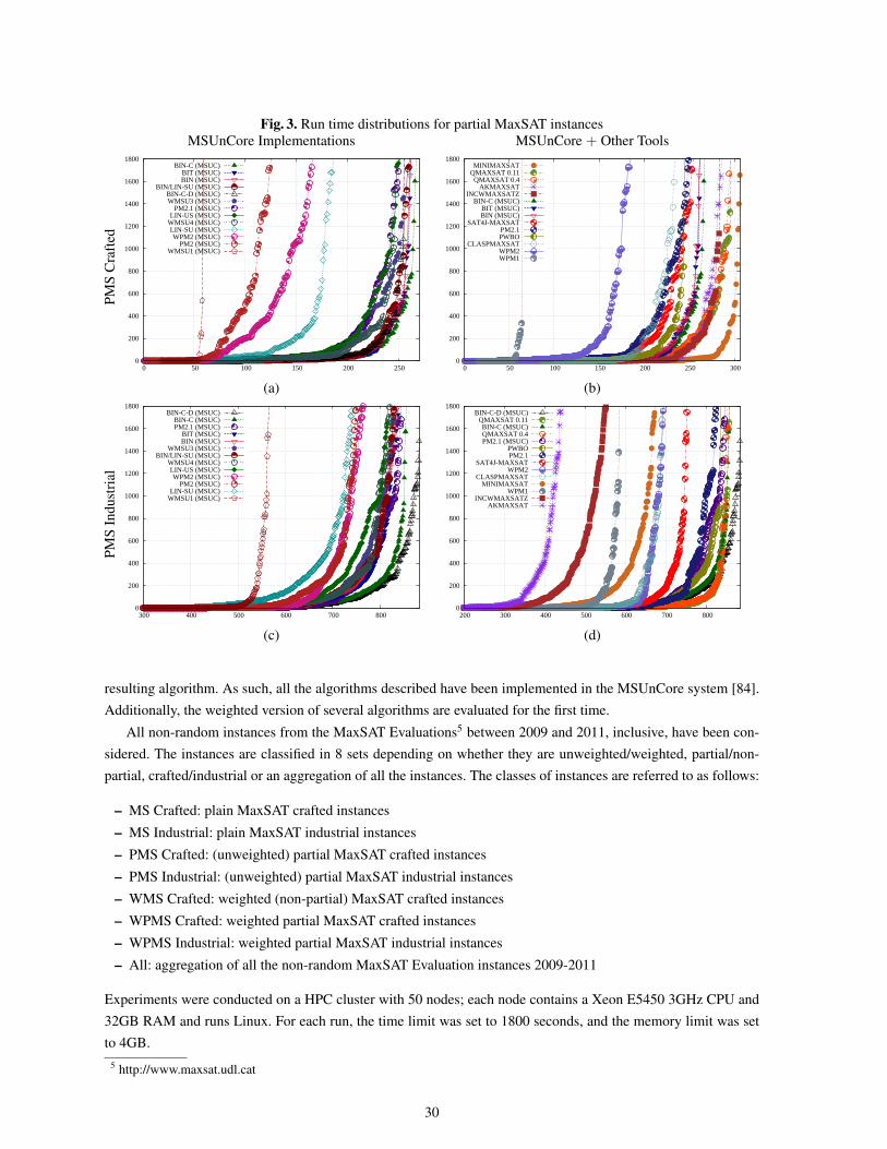
Fig. 3. Run time distributions for partial MaxSAT instances


PM

SC

raft

ed

0

200

400

600

800

1000

1200

1400

1600

1800

0 50 100 150 200 250

BIN-C (MSUC)BIT (MSUC)BIN (MSUC)

BIN/LIN-SU (MSUC)BIN-C-D (MSUC)WMSU3 (MSUC)

PM2.1 (MSUC)LIN-US (MSUC)

WMSU4 (MSUC)LIN-SU (MSUC)WPM2 (MSUC)

PM2 (MSUC)WMSU1 (MSUC)

0

200

400

600

800

1000

1200

1400

1600

1800

0 50 100 150 200 250 300

MINIMAXSATQMAXSAT 0.11QMAXSAT 0.4

AKMAXSATINCWMAXSATZ

BIN-C (MSUC)BIT (MSUC)BIN (MSUC)

SAT4J-MAXSATPM2.1PWBO

CLASPMAXSATWPM2WPM1

(a) (b)

PM

SIn

dust

rial

0

200

400

600

800

1000

1200

1400

1600

1800

300 400 500 600 700 800

BIN-C-D (MSUC)BIN-C (MSUC)PM2.1 (MSUC)

BIT (MSUC)BIN (MSUC)

WMSU3 (MSUC)BIN/LIN-SU (MSUC)

WMSU4 (MSUC)LIN-US (MSUC)WPM2 (MSUC)

PM2 (MSUC)LIN-SU (MSUC)

WMSU1 (MSUC)

0

200

400

600

800

1000

1200

1400

1600

1800

200 300 400 500 600 700 800

BIN-C-D (MSUC)QMAXSAT 0.11BIN-C (MSUC)QMAXSAT 0.4PM2.1 (MSUC)

PWBOPM2.1

SAT4J-MAXSATWPM2

CLASPMAXSATMINIMAXSAT

WPM1INCWMAXSATZ

AKMAXSAT

(c) (d)

resulting algorithm. As such, all the algorithms described have been implemented in the MSUnCore system [84].

Additionally, the weighted version of several algorithms are evaluated for the first time.

All non-random instances from the MaxSAT Evaluations5 between 2009 and 2011, inclusive, have been con-

sidered. The instances are classified in 8 sets depending on whether they are unweighted/weighted, partial/non-

partial, crafted/industrial or an aggregation of all the instances. The classes of instances are referred to as follows:

– MS Crafted: plain MaxSAT crafted instances

– MS Industrial: plain MaxSAT industrial instances

– PMS Crafted: (unweighted) partial MaxSAT crafted instances

– PMS Industrial: (unweighted) partial MaxSAT industrial instances

– WMS Crafted: weighted (non-partial) MaxSAT crafted instances

– WPMS Crafted: weighted partial MaxSAT crafted instances

– WPMS Industrial: weighted partial MaxSAT industrial instances

– All: aggregation of all the non-random MaxSAT Evaluation instances 2009-2011

Experiments were conducted on a HPC cluster with 50 nodes; each node contains a Xeon E5450 3GHz CPU and

32GB RAM and runs Linux. For each run, the time limit was set to 1800 seconds, and the memory limit was set

to 4GB.

5 http://www.maxsat.udl.cat

30

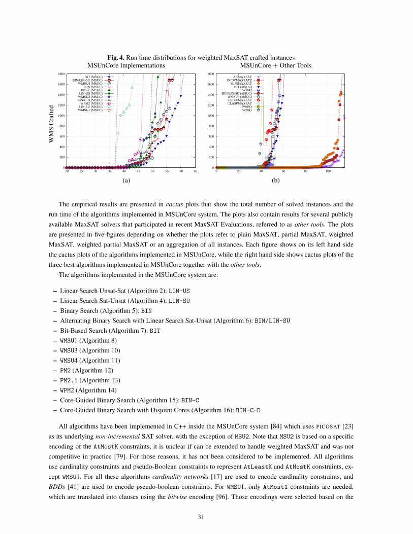
Fig. 4. Run time distributions for weighted MaxSAT crafted instances


WM

SC

raft

ed

0

200

400

600

800

1000

1200

1400

1600

1800

20 25 30 35 40 45 50 55 60 65

BIT (MSUC)BIN/LIN-SU (MSUC)

WMSU4 (MSUC)BIN (MSUC)

BIN-C (MSUC)LIN-US (MSUC)

WMSU3 (MSUC)BIN-C-D (MSUC)

WPM2 (MSUC)LIN-SU (MSUC)

WMSU1 (MSUC)

0

200

400

600

800

1000

1200

1400

1600

1800

0 20 40 60 80 100

AKMAXSATINCWMAXSATZ

MINIMAXSATBIT (MSUC)

WPM2BIN/LIN-SU (MSUC)

WMSU4 (MSUC)SAT4J-MAXSATCLASPMAXSAT

PWBOWPM1

(a) (b)

The empirical results are presented in cactus plots that show the total number of solved instances and the

run time of the algorithms implemented in MSUnCore system. The plots also contain results for several publicly

available MaxSAT solvers that participated in recent MaxSAT Evaluations, referred to as other tools. The plots

are presented in five figures depending on whether the plots refer to plain MaxSAT, partial MaxSAT, weighted

MaxSAT, weighted partial MaxSAT or an aggregation of all instances. Each figure shows on its left hand side

the cactus plots of the algorithms implemented in MSUnCore, while the right hand side shows cactus plots of the

three best algorithms implemented in MSUnCore together with the other tools.

The algorithms implemented in the MSUnCore system are:

– Linear Search Unsat-Sat (Algorithm 2): LIN-US

– Linear Search Sat-Unsat (Algorithm 4): LIN-SU

– Binary Search (Algorithm 5): BIN

– Alternating Binary Search with Linear Search Sat-Unsat (Algorithm 6): BIN/LIN-SU

– Bit-Based Search (Algorithm 7): BIT

– WMSU1 (Algorithm 8)



– PM2 (Algorithm 12)

– PM2.1 (Algorithm 13)

– WPM2 (Algorithm 14)

– Core-Guided Binary Search (Algorithm 15): BIN-C

– Core-Guided Binary Search with Disjoint Cores (Algorithm 16): BIN-C-D

All algorithms have been implemented in C++ inside the MSUnCore system [84] which uses PICOSAT [23]

as its underlying non-incremental SAT solver, with the exception of MSU2. Note that MSU2 is based on a specific

encoding of the AtMostK constraints, it is unclear if can be extended to handle weighted MaxSAT and was not

competitive in practice [79]. For those reasons, it has not been considered to be implemented. All algorithms

use cardinality constraints and pseudo-Boolean constraints to represent AtLeastK and AtMostK constraints, ex-

cept WMSU1. For all these algorithms cardinality networks [17] are used to encode cardinality constraints, and

BDDs [41] are used to encode pseudo-boolean constraints. For WMSU1, only AtMost1 constraints are needed,

which are translated into clauses using the bitwise encoding [96]. Those encodings were selected based on the

31

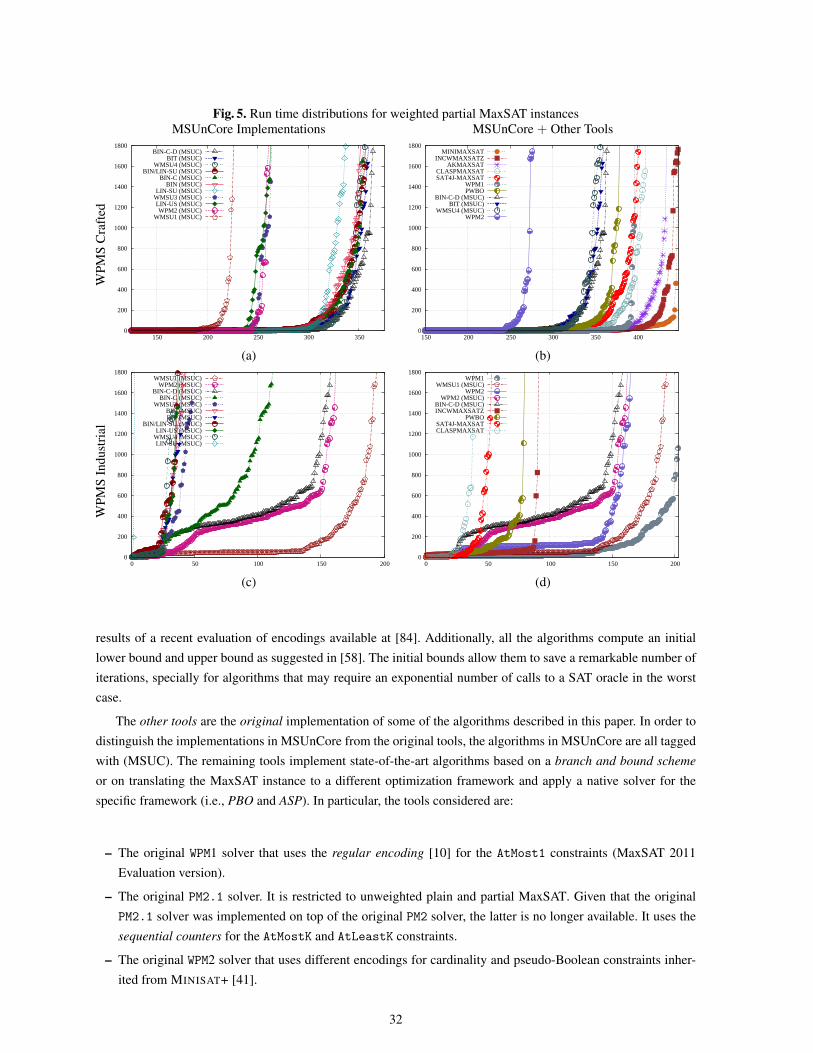
Fig. 5. Run time distributions for weighted partial MaxSAT instances


WP

MS

Cra

fted

0

200

400

600

800

1000

1200

1400

1600

1800

150 200 250 300 350

BIN-C-D (MSUC)BIT (MSUC)

WMSU4 (MSUC)BIN/LIN-SU (MSUC)

BIN-C (MSUC)BIN (MSUC)

LIN-SU (MSUC)WMSU3 (MSUC)LIN-US (MSUC)WPM2 (MSUC)

WMSU1 (MSUC)

0

200

400

600

800

1000

1200

1400

1600

1800

150 200 250 300 350 400

MINIMAXSATINCWMAXSATZ

AKMAXSATCLASPMAXSATSAT4J-MAXSAT

WPM1PWBO

BIN-C-D (MSUC)BIT (MSUC)

WMSU4 (MSUC)WPM2

(a) (b)

WP

MS

Indust

rial

0

200

400

600

800

1000

1200

1400

1600

1800

0 50 100 150 200

WMSU1 (MSUC)WPM2 (MSUC)

BIN-C-D (MSUC)BIN-C (MSUC)

WMSU3 (MSUC)BIN (MSUC)BIT (MSUC)

BIN/LIN-SU (MSUC)LIN-US (MSUC)

WMSU4 (MSUC)LIN-SU (MSUC)

0

200

400

600

800

1000

1200

1400

1600

1800

0 50 100 150 200

WPM1WMSU1 (MSUC)

WPM2WPM2 (MSUC)

BIN-C-D (MSUC)INCWMAXSATZ

PWBOSAT4J-MAXSATCLASPMAXSAT

(c) (d)

results of a recent evaluation of encodings available at [84]. Additionally, all the algorithms compute an initial

lower bound and upper bound as suggested in [58]. The initial bounds allow them to save a remarkable number of

iterations, specially for algorithms that may require an exponential number of calls to a SAT oracle in the worst

case.

The other tools are the original implementation of some of the algorithms described in this paper. In order to

distinguish the implementations in MSUnCore from the original tools, the algorithms in MSUnCore are all tagged

with (MSUC). The remaining tools implement state-of-the-art algorithms based on a branch and bound scheme

or on translating the MaxSAT instance to a different optimization framework and apply a native solver for the

specific framework (i.e., PBO and ASP). In particular, the tools considered are:

– The original WPM1 solver that uses the regular encoding [10] for the AtMost1 constraints (MaxSAT 2011

Evaluation version).

– The original PM2.1 solver. It is restricted to unweighted plain and partial MaxSAT. Given that the original

PM2.1 solver was implemented on top of the original PM2 solver, the latter is no longer available. It uses the

sequential counters for the AtMostK and AtLeastK constraints.

– The original WPM2 solver that uses different encodings for cardinality and pseudo-Boolean constraints inher-

ited from MINISAT+ [41].

32

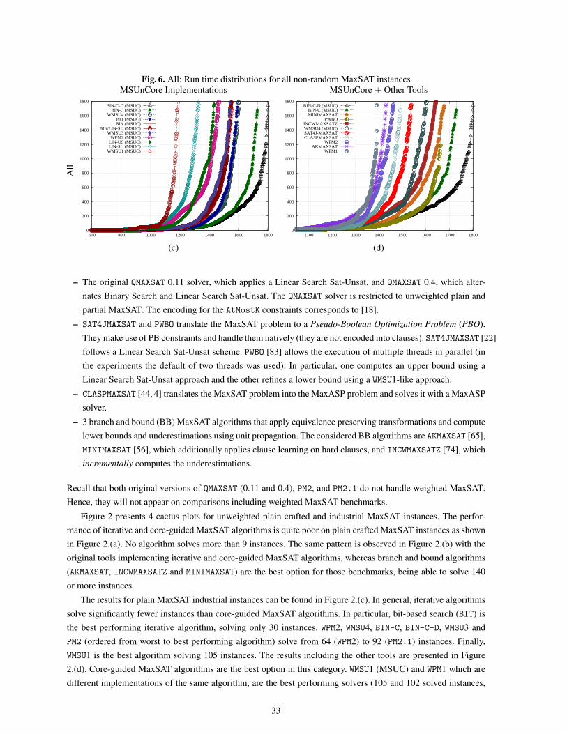
Fig. 6. All: Run time distributions for all non-random MaxSAT instances


All

0

200

400

600

800

1000

1200

1400

1600

1800

600 800 1000 1200 1400 1600 1800

BIN-C-D (MSUC)BIN-C (MSUC)

WMSU4 (MSUC)BIT (MSUC)BIN (MSUC)

BIN/LIN-SU (MSUC)WMSU3 (MSUC)

WPM2 (MSUC)LIN-US (MSUC)LIN-SU (MSUC)

WMSU1 (MSUC)

0

200

400

600

800

1000

1200

1400

1600

1800

1100 1200 1300 1400 1500 1600 1700 1800

BIN-C-D (MSUC)BIN-C (MSUC)MINIMAXSAT

PWBOINCWMAXSATZWMSU4 (MSUC)SAT4J-MAXSATCLASPMAXSAT

WPM2AKMAXSAT

WPM1

(c) (d)

– The original QMAXSAT 0.11 solver, which applies a Linear Search Sat-Unsat, and QMAXSAT 0.4, which alter-

nates Binary Search and Linear Search Sat-Unsat. The QMAXSAT solver is restricted to unweighted plain and

partial MaxSAT. The encoding for the AtMostK constraints corresponds to [18].

– SAT4JMAXSAT and PWBO translate the MaxSAT problem to a Pseudo-Boolean Optimization Problem (PBO).

They make use of PB constraints and handle them natively (they are not encoded into clauses). SAT4JMAXSAT [22]

follows a Linear Search Sat-Unsat scheme. PWBO [83] allows the execution of multiple threads in parallel (in

the experiments the default of two threads was used). In particular, one computes an upper bound using a

Linear Search Sat-Unsat approach and the other refines a lower bound using a WMSU1-like approach.

– CLASPMAXSAT [44, 4] translates the MaxSAT problem into the MaxASP problem and solves it with a MaxASP

solver.

– 3 branch and bound (BB) MaxSAT algorithms that apply equivalence preserving transformations and compute

lower bounds and underestimations using unit propagation. The considered BB algorithms are AKMAXSAT [65],

MINIMAXSAT [56], which additionally applies clause learning on hard clauses, and INCWMAXSATZ [74], which

incrementally computes the underestimations.

Recall that both original versions of QMAXSAT (0.11 and 0.4), PM2, and PM2.1 do not handle weighted MaxSAT.

Hence, they will not appear on comparisons including weighted MaxSAT benchmarks.

Figure 2 presents 4 cactus plots for unweighted plain crafted and industrial MaxSAT instances. The perfor-

mance of iterative and core-guided MaxSAT algorithms is quite poor on plain crafted MaxSAT instances as shown

in Figure 2.(a). No algorithm solves more than 9 instances. The same pattern is observed in Figure 2.(b) with the

original tools implementing iterative and core-guided MaxSAT algorithms, whereas branch and bound algorithms

(AKMAXSAT, INCWMAXSATZ and MINIMAXSAT) are the best option for those benchmarks, being able to solve 140

or more instances.

The results for plain MaxSAT industrial instances can be found in Figure 2.(c). In general, iterative algorithms

solve significantly fewer instances than core-guided MaxSAT algorithms. In particular, bit-based search (BIT) is

the best performing iterative algorithm, solving only 30 instances. WPM2, WMSU4, BIN-C, BIN-C-D, WMSU3 and

PM2 (ordered from worst to best performing algorithm) solve from 64 (WPM2) to 92 (PM2.1) instances. Finally,

WMSU1 is the best algorithm solving 105 instances. The results including the other tools are presented in Figure

2.(d). Core-guided MaxSAT algorithms are the best option in this category. WMSU1 (MSUC) and WPM1 which are

different implementations of the same algorithm, are the best performing solvers (105 and 102 solved instances,

33

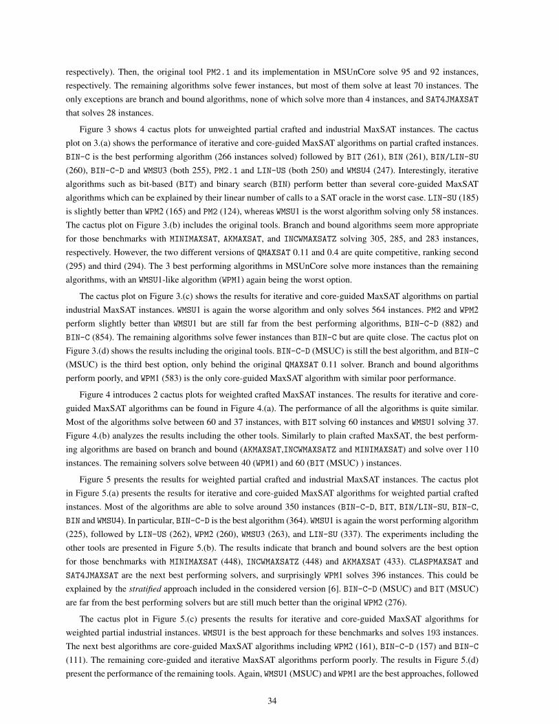
respectively). Then, the original tool PM2.1 and its implementation in MSUnCore solve 95 and 92 instances,

respectively. The remaining algorithms solve fewer instances, but most of them solve at least 70 instances. The

only exceptions are branch and bound algorithms, none of which solve more than 4 instances, and SAT4JMAXSAT

that solves 28 instances.

Figure 3 shows 4 cactus plots for unweighted partial crafted and industrial MaxSAT instances. The cactus

plot on 3.(a) shows the performance of iterative and core-guided MaxSAT algorithms on partial crafted instances.

BIN-C is the best performing algorithm (266 instances solved) followed by BIT (261), BIN (261), BIN/LIN-SU

(260), BIN-C-D and WMSU3 (both 255), PM2.1 and LIN-US (both 250) and WMSU4 (247). Interestingly, iterative

algorithms such as bit-based (BIT) and binary search (BIN) perform better than several core-guided MaxSAT

algorithms which can be explained by their linear number of calls to a SAT oracle in the worst case. LIN-SU (185)

is slightly better than WPM2 (165) and PM2 (124), whereas WMSU1 is the worst algorithm solving only 58 instances.

The cactus plot on Figure 3.(b) includes the original tools. Branch and bound algorithms seem more appropriate

for those benchmarks with MINIMAXSAT, AKMAXSAT, and INCWMAXSATZ solving 305, 285, and 283 instances,

respectively. However, the two different versions of QMAXSAT 0.11 and 0.4 are quite competitive, ranking second

(295) and third (294). The 3 best performing algorithms in MSUnCore solve more instances than the remaining

algorithms, with an WMSU1-like algorithm (WPM1) again being the worst option.

The cactus plot on Figure 3.(c) shows the results for iterative and core-guided MaxSAT algorithms on partial

industrial MaxSAT instances. WMSU1 is again the worse algorithm and only solves 564 instances. PM2 and WPM2

perform slightly better than WMSU1 but are still far from the best performing algorithms, BIN-C-D (882) and

BIN-C (854). The remaining algorithms solve fewer instances than BIN-C but are quite close. The cactus plot on

Figure 3.(d) shows the results including the original tools. BIN-C-D (MSUC) is still the best algorithm, and BIN-C

(MSUC) is the third best option, only behind the original QMAXSAT 0.11 solver. Branch and bound algorithms

perform poorly, and WPM1 (583) is the only core-guided MaxSAT algorithm with similar poor performance.

Figure 4 introduces 2 cactus plots for weighted crafted MaxSAT instances. The results for iterative and core-

guided MaxSAT algorithms can be found in Figure 4.(a). The performance of all the algorithms is quite similar.

Most of the algorithms solve between 60 and 37 instances, with BIT solving 60 instances and WMSU1 solving 37.

Figure 4.(b) analyzes the results including the other tools. Similarly to plain crafted MaxSAT, the best perform-

ing algorithms are based on branch and bound (AKMAXSAT,INCWMAXSATZ and MINIMAXSAT) and solve over 110

instances. The remaining solvers solve between 40 (WPM1) and 60 (BIT (MSUC) ) instances.

Figure 5 presents the results for weighted partial crafted and industrial MaxSAT instances. The cactus plot

in Figure 5.(a) presents the results for iterative and core-guided MaxSAT algorithms for weighted partial crafted

instances. Most of the algorithms are able to solve around 350 instances (BIN-C-D, BIT, BIN/LIN-SU, BIN-C,

BIN and WMSU4). In particular, BIN-C-D is the best algorithm (364). WMSU1 is again the worst performing algorithm

(225), followed by LIN-US (262), WPM2 (260), WMSU3 (263), and LIN-SU (337). The experiments including the

other tools are presented in Figure 5.(b). The results indicate that branch and bound solvers are the best option

for those benchmarks with MINIMAXSAT (448), INCWMAXSATZ (448) and AKMAXSAT (433). CLASPMAXSAT and

SAT4JMAXSAT are the next best performing solvers, and surprisingly WPM1 solves 396 instances. This could be

explained by the stratified approach included in the considered version [6]. BIN-C-D (MSUC) and BIT (MSUC)

are far from the best performing solvers but are still much better than the original WPM2 (276).

The cactus plot in Figure 5.(c) presents the results for iterative and core-guided MaxSAT algorithms for

weighted partial industrial instances. WMSU1 is the best approach for these benchmarks and solves 193 instances.

The next best algorithms are core-guided MaxSAT algorithms including WPM2 (161), BIN-C-D (157) and BIN-C

(111). The remaining core-guided and iterative MaxSAT algorithms perform poorly. The results in Figure 5.(d)

present the performance of the remaining tools. Again, WMSU1 (MSUC) and WPM1 are the best approaches, followed

34

by WPM2 / WPM2 (MSUC) and BIN-C-D (MSUC) as in the previous plot. The remaining approaches including

branch and bound algorithms, PBO, and ASP tools are quite far from the best performing algorithms.

Figure 6 introduces 2 cactus plots aggregating all of the instances considered. The cactus plot in Figure 6.(a)

shows the results for iterative and core-guided MaxSAT algorithms. The best overall performing algorithm is

BIN-C-D followed by BIN-C. The third best solver is WMSU4 and it is followed by other algorithms which compute

a middle value between a lower bound and upper bound. Algorithms based on exclusively refining a lower bound

or an upper bound perform worse. Whereas WMSU1 is the overall second worst solver, recall that it is in fact the

best approach in two industrial categories.

The cactus plot in Figure 6.(b) shows the results for the other tools. Again, BIN-C-D (MSUC) and BIN-C

(MSUC) are the overall best algorithms. From these results, several conclusions can be extracted. First, core-

guided MaxSAT algorithms perform better than classic iterative algorithms. Branch and bound algorithms are

more appropriate for crafted instances, specially on non-partial benchmarks. However, iterative and core-guided

MaxSAT algorithms also achieve very good performance on partial crafted instances. For industrial instances,

core-guided MaxSAT algorithms are the most effective; WMSU1-like algorithms are the best option for unweighted

plain and weighted partial MaxSAT instances, and core-guided binary search with disjoint cores (BIN-C-D) is the

best approach for unweighted partial MaxSAT. Finally, the most robust approach overall is BIN-C-D.

7 Conclusions

MaxSAT is an optimization variant of the Satisfiability problem that finds a wide range of applications. In par-

ticular, MaxSAT has recently been applied in industrial contexts including Design Debugging [102, 30], Fault

Localization of ANSI-C Programs [61, 62], Post-Silicon Validation [120], Planning [34, 63, 118, 99], and Model-

Based-Diagnosis [42], to name a few.

In the last decade, a large number of exact algorithms have been proposed for MaxSAT, some of which are

based on iteratively calling a SAT solver and are called iterative MaxSAT solvers. Exploiting the ability of SAT

solvers to compute reasons for unsatisfiable formulas (unsatisfiable cores), new approaches for MaxSAT solving

have emerged that take advantage of the presence of cores to further enhance their performance. These algorithms

are called core-guided MaxSAT algorithms.

This paper overviews existing iterative and core-guided MaxSAT algorithms and characterizes them in terms

of number of relaxation variables, number of constraints and number of calls to a SAT oracle. Additionally, several

algorithms originally available only for unweighted MaxSAT have been extended to handle weighted formulas.

Iterative algorithms initially relax all soft clauses. Then, they iteratively add a cardinality constraint on the

number of relaxation variables allowed to be assigned true and call a SAT solver. In the case of weighted versions

of the algorithms, instead of the cardinality constraint, a pseudo-Boolean constraint is added that constrains the

allowed weight of the associated cost function. Core-guided MaxSAT algorithms compute unsatisfiable cores

when the outcome of the SAT solver is unsatisfiable, and use the information of unsatisfiable cores to relax soft

clauses on demand and to compute more precise and smaller constraints.

An extensive empirical study has been conducted that considers all non-random instances from recent MaxSAT

Evaluations, the surveyed algorithms and other state-of-the-art approaches such as branch and bound MaxSAT

solvers, pseudo-Boolean solvers and ASP solvers. The iterative and core-guided MaxSAT algorithms were de-

veloped in the same implementation framework, which allows for a fair comparison of all algorithmic schemes

independently of implementation details. Both original (if any) and our own implementation of each iterative and

core-guided MaxSAT algorithm were considered. Branch and bound algorithms [74, 56, 65] are known to be the

best complete approach to handle random benchmarks, and the results in this paper indicate that they are also

the best approach to handle non-partial crafted benchmarks. Differently, for crafted partial benchmarks iterative

35

and core-guided MaxSAT algorithms are quite competitive. Regarding industrial (partial and non-partial) bench-

marks, core-guided MaxSAT algorithms followed by iterative MaxSAT algorithms are among the best approaches,

whereas branch and bound algorithms perform poorly. In fact, the results indicate that WMSU1 / WPM1 is the best

approach to handle industrial unweighted MaxSAT and weighted partial industrial MaxSAT, whereas core-guided

binary search with disjoint cores is the best approach for partial MaxSAT industrial benchmarks and it is quite ro-

bust in general. Hence, in general the results indicate that core-guided MaxSAT algorithms are better than iterative

algorithms and that core-guided MaxSAT algorithms are fairly competitive compared to the remaining approaches

and the current best approach for industrial benchmarks.

Acknowledgement. This work is partially supported by SFI grant BEACON (09/PI/I2618).

References

1. L. Aksoy, E. A. C. da Costa, P. F. Flores, and J. Monteiro. Exact and approximate algorithms for the optimization of area

and delay in multiple constant multiplications. IEEE Transactions on CAD of Integrated Circuits and Systems on CAD,

27(6):1013–1026, 2008.

2. F. Aloul, A. Ramani, I. Markov, and K. Sakallah. PBS: A backtrack search pseudo-boolean solver. In Symp. Theory and

Applications of Satisfiability Testing, pages 346–353, 2002.

3. F. A. Aloul, A. Ramani, I. L. Markov, and K. A. Sakallah. Generic ILP versus specialized 0-1 ILP: an update. In

International Conference on Computer-Aided Design, pages 450–457, November 2002.

4. B. Andres, B. Kaufmann, O. Matheis, and T. Schaub. Unsatisfiability-based optimization in clasp. In ICLP (Technical

Communications), pages 211–221, 2012.

5. M. F. Anjos. Semidefinite optimization approaches for satisfiability and maximum-satisfiability problems. JSAT, 1(1):1–

47, 2006.

6. C. Ansotegui, M. L. Bonet, J. Gabas, and J. Levy. Improving sat-based weighted MaxSAT solvers. In International

Conference on Principles and Practice of Constraint Programming, 2012.

7. C. Ansotegui, M. L. Bonet, and J. Levy. On solving MaxSAT through SAT. In CCIA, pages 284–292, 2009.

8. C. Ansotegui, M. L. Bonet, and J. Levy. Solving (weighted) partial MaxSAT through satisfiability testing. In Theory and

Applications of Satisfiability Testing, pages 427–440, July 2009.

9. C. Ansotegui, M. L. Bonet, and J. Levy. A new algorithm for weighted partial MaxSAT. In AAAI Conference on Artificial

Intelligence. AAAI, 2010.

10. C. Ansotegui and F. Manya. Mapping problems with finite-domain variables into problems with Boolean variables. In

SAT, 2004.

11. C. A. Ardagna, S. D. C. di Vimercati, S. Foresti, S. Paraboschi, and P. Samarati. Minimizing disclosure of private

information in credential-based interactions: A graph-based approach. In International Conference on Social Computing

/ International Conference on Privacy, Security, Risk and Trust, pages 743–750, 2010.

12. J. Argelich, D. L. Berre, I. Lynce, J. Marques-Silva, and P. Rapicault. Solving linux upgradeability problems using

boolean optimization. In International Workshop on Logics for Component Configuration, pages 11–22, 2010.

13. J. Argelich and I. Lynce. CNF instances from the software package installation problem. In RCRA Workshop, 2008.

14. J. Argelich, I. Lynce, and J. Marques-Silva. On solving Boolean multilevel optimization problems. In International Joint

Conference on Artificial Intelligence, pages 393–398, July 2009.

15. R. Asin and R. Nieuwenhuis. Curriculum-based course timetabling with sat and maxsat. In International Conference on

the Practice and Theory of Automated Timetabling, 2010.

16. R. Asin and R. Nieuwenhuis. Curriculum-based course timetabling with sat and maxsat. Annals of Operations Research,

2012.

17. R. Asın, R. Nieuwenhuis, A. Oliveras, and E. Rodrıguez-Carbonell. Cardinality networks: a theoretical and empirical

study. Constraints, pages 1–27, 2011.

18. O. Bailleux and Y. Boufkhad. Efficient CNF encoding of Boolean cardinality constraints. In CP, pages 108–122, 2003.

36

19. N. Bansal and V. Raman. Upper bounds for MaxSat: Further improved. In ISAAC, pages 247–258, 1999.

20. C. Barrett, R. Sebastiani, S. A. Seshia, and C. Tinelli. Satisfiability modulo theories. In Handbook of Satisfiability, pages

825–884. IOS Press, 2009.

21. P. Barth. A davis-putnam enumeration algorithm for linear pseudo-Boolean optimization. Technical Report MPI-I-95-2-

003, Max Plank Institute for Computer Science, 1995.

22. D. L. Berre and A. Parrain. The sat4j library, release 2.2. JSAT, 7:59–64, 2010.

23. A. Biere. PicoSAT essentials. Journal on Satisfiability, Boolean Modeling and Computation, 2:75–97, 2008.

24. E. Birnbaum and E. L. Lozinskii. Consistent subsets of inconsistent systems: structure and behaviour. Journal of

Experimental and Theoretical Artificial Intelligence, 15(1):25–46, 2003.

25. M. L. Bonet, J. Levy, and F. Manya. Resolution for Max-SAT. Artificial Intelligence, 171(8–9):606–618, 2007.

26. B. Borchers and J. Furman. A two-phase exact algorithm for MAX-SAT and weighted MAX-SAT problems. Journal of

Combinatorial Optimization, 2:299–306, 1999.

27. T. Brihaye, V. Bruyere, L. Doyen, M. Ducobu, and J.-F. Raskin. Antichain-based qbf solving. In International Symposium

on Automated Technology for Verification and Analysis, pages 183–197, 2011.

28. B. Cha, K. Iwama, Y. Kambayashi, and S. Miyazaki. Local search algorithms for partial maxsat. In AAAI/IAAI, pages

263–268, 1997.

29. D. Chai and A. Kuehlmann. A fast pseudo-Boolean constraint solver. In Design Automation Conference, pages 830–835,

2003.

30. Y. Chen, S. Safarpour, J. Marques-Silva, and A. G. Veneris. Automated design debugging with maximum satisfiability.

IEEE Transactions on CAD of Integrated Circuits and Systems, 29(11):1804–1817, 2010.

31. Y. Chen, S. Safarpour, A. Veneris, and J. Marques-Silva. Spatial and temporal design debug using partial MaxSAT. In

IEEE Great Lakes Symposium on VLSI, July 2009.

32. A. Cimatti, A. Franzen, A. Griggio, R. Sebastiani, and C. Stenico. Satisfiability modulo the theory of costs: Foundations

and applications. In TACAS, pages 99–113, 2010.

33. M. Codish, V. Lagoon, and P. J. Stuckey. Logic programming with satisfiability. TPLP, 8(1):121–128, 2008.

34. M. C. Cooper, S. Cussat-Blanc, M. de Roquemaurel, and P. Regnier. Soft arc consistency applied to optimal planning.

In International Conference on Principles and Practice of Constraint Programming, pages 680–684, September 2006.

35. M. C. Cooper, S. de Givry, M. Sanchez, T. Schiex, M. Zytnicki, and T. Werner. Soft arc consistency revisited. Artif.

Intell., 174(7-8):449–478, 2010.

36. J. Davies and F. Bacchus. Solving MaxSAT by solving a sequence of simpler SAT instances. In International Conference

on Principles and Practice of Constraint Programming, pages 225–239, 2011.

37. J. Davies, J. Cho, and F. Bacchus. Using learnt clauses in maxsat. In CP, pages 176–190, 2010.

38. S. de Givry, J. Larrosa, P. Meseguer, and T. Schiex. Solving Max-SAT as weighted CSP. In International Conference on

Principles and Practice of Constraint Programming, pages 363–376, 2003.

39. L. M. de Moura and N. Bjørner. Z3: An efficient SMT solver. In TACAS, pages 337–340, 2008.

40. N. Een and N. Sorensson. An extensible sat-solver. In SAT, pages 502–518, 2003.

41. N. Een and N. Sorensson. Translating pseudo-Boolean constraints into SAT. Journal on Satisfiability, Boolean Modeling

and Computation, 2:1–26, 2006.

42. A. Feldman, G. Provan, J. de Kleer, S. Robert, and A. van Gemund. Solving model-based diagnosis problems with

MaxSAT solvers and vice versa. In International Workshop on the Principles of Diagnosis, 2010.

43. Z. Fu and S. Malik. On solving the partial MAX-SAT problem. In Theory and Applications of Satisfiability Testing,

pages 252–265, August 2006.

44. M. Gebser, B. Kaufmann, and T. Schaub. The conflict-driven answer set solver clasp: Progress report. In LPNMR, pages

509–514, 2009.

45. E. Giunchiglia, Y. Lierler, and M. Maratea. Answer set programming based on propositional satisfiability. J. Autom.

Reasoning, 36(4):345–377, 2006.

46. E. Giunchiglia and M. Maratea. optsat: A tool for solving sat related optimization problems. In European Conference

on Logics in Artificial Intelligence (JELIA), pages 485–489, 2006.

47. E. Giunchiglia and M. Maratea. Solving optimization problems with DLL. In European Conference on Artificial Intelli-

gence, pages 377–381, August 2006.

37

48. E. Giunchiglia and M. Maratea. Planning as satisfiability with preferences. In AAAI Conference on Artificial Intelligence,

pages 987–992, 2007.

49. C. P. Gomes, W. J. van Hoeve, and L. Leahu. The power of semidefinite programming relaxations for max-sat. In

CPAIOR, pages 104–118, 2006.

50. G. Gottlob. Np trees and carnap’s modal logic. J. ACM, 42(2):421–457, 1995.

51. A. Graca, I. Lynce, J. Marques-Silva, and A. Oliveira. Efficient and accurate haplotype inference by combining parsimony

and pedigree information. In International Conference Algebraic and Numeric Biology, pages 38–56, 2010.

52. A. Graca, J. Marques-Silva, I. Lynce, and A. Oliveira. Haplotype inference with pseudo-boolean optimization. Annals

of Operations Research, 184(1):137–162, 2011.

53. J. Guerra and I. Lynce. Reasoning over biological networks using maximum satisfiability. In CP, pages 941–956, 2012.

54. G. D. Hachtel and F. Somenzi. Logic synthesis and verification algorithms. Kluwer, 1996.

55. F. Heras, J. Larrosa, S. de Givry, and T. Schiex. 2006 and 2007 Max-SAT evaluations: Contributed instances. Journal on

Satisfiability, Boolean Modeling and Computation, 4(2-4):239–250, June 2008.

56. F. Heras, J. Larrosa, and A. Oliveras. MiniMaxSat: An efficient weighted Max-SAT solver. Journal of Artificial Intelli-

gence Research, 31:1–32, January 2008.

57. F. Heras and J. Marques-Silva. Read-once resolution for unsatisfiability-based Max-SAT algorithms. In IJCAI, pages

572–577, 2011.

58. F. Heras, A. Morgado, and J. Marques-Silva. Core-guided binary search for maximum satisfiability. In AAAI Conference

on Artificial Intelligence. AAAI, 2011.

59. H. Hoos and T. Stutzle. Stochastic Local Search: Foundations and Applications. Morgan Kaufmann, 2005.

60. H. H. Hoos. An adaptive noise mechanism for WalkSAT. In AAAI/IAAI, pages 655–660, 2002.

61. M. Jose and R. Majumdar. Bug-assist: Assisting fault localization in ansi-c programs. In CAV, pages 504–509, 2011.

62. M. Jose and R. Majumdar. Cause clue clauses: error localization using maximum satisfiability. In PLDI, pages 437–446,

2011.

63. F. Juma, E. I. Hsu, and S. A. McIlraith. Preference-based planning via maxsat. In Canadian Conference on AI, pages

109–120, 2012.

64. M. Koshimura, T. Zhang, H. Fujita, and R. Hasegawa. Qmaxsat: A partial Max-SAT solver. JSAT, 8:95–100, 2012.

65. A. Kuegel. Improved exact solver for the weighted MAX-SAT problem. In Pragmatics of SAT, 2010.

66. J. Larrosa and F. Heras. Resolution in max-sat and its relation to local consistency in weighted csps. In IJCAI, pages

193–198, 2005.

67. J. Larrosa, F. Heras, and S. de Givry. A logical approach to efficient Max-SAT solving. Artificial Intelligence, 172(2-

3):204–233, 2008.

68. J. Larrosa and T. Schiex. Solving weighted CSP by maintaining arc consistency. Artif. Intell., 159(1-2):1–26, 2004.

69. C. M. Li and F. Manya. MaxSAT, hard and soft constraints. In Handbook of Satisfiability, pages 613–632. IOS Press,

2009.

70. C. M. Li, F. Manya, and J. Planes. Exploiting unit propagation to compute lower bounds in branch and bound Max-SAT

solvers. In International Conference on Principles and Practice of Constraint Programming, pages 403–414, 2005.

71. C. M. Li, F. Manya, and J. Planes. New inference rules for Max-SAT. Journal of Artificial Intelligence Research,

30:321–359, October 2007.

72. M. H. Liffiton and K. A. Sakallah. On finding all minimally unsatisfiable subformulas. In International Conference on

Theory and Applications of Satisfiability Testing, pages 173–186, June 2005.

73. M. H. Liffiton and K. A. Sakallah. Algorithms for computing minimal unsatisfiable subsets of constraints. Journal

Automated Reasoning, 40(1):1–33, 2008.

74. H. Lin, K. Su, and C. M. Li. Within-problem learning for efficient lower bound computation in Max-SAT solving. In

AAAI, pages 351–356, 2008.

75. F. Mancinelli, J. Boender, R. di Cosmo, J. Vouillon, B. Durak, X. Leroy, and R. Treinen. Managing the complexity

of large free and open source package-based software distributions. In Int. Conf. Automated Soft. Engineering, pages

199–208, 2006.

76. H. Mangassarian, A. G. Veneris, S. Safarpour, F. N. Najm, and M. S. Abadir. Maximum circuit activity estimation using

pseudo-boolean satisfiability. In Design, Automation and Test in Europe Conference, pages 1538–1543, 2007.

38

77. V. Manquinho, J. Marques-Silva, and J. Planes. Algorithms for weighted Boolean optimization. In Theory and Applica-

tions of Satisfiability Testing, pages 495–508, July 2009.

78. J. Marques-Silva, J. Argelich, A. Graca, and I. Lynce. Boolean lexicographic optimization: algorithms & applications.

Ann. Math. Artif. Intell., 62(3-4):317–343, 2011.

79. J. Marques-Silva and V. Manquinho. Towards more effective unsatisfiability-based maximum satisfiability algorithms.

In Theory and Applications of Satisfiability Testing, pages 225–230, March 2008.

80. J. Marques-Silva and J. Planes. On using unsatisfiability for solving maximum satisfiability. Computing Research

Repository, abs/0712.0097, December 2007.

81. J. Marques-Silva and J. Planes. Algorithms for maximum satisfiability using unsatisfiable cores. In Design, Automation

and Testing in Europe Conference, pages 408–413, March 2008.

82. R. Martins, V. Manquinho, and I. Lynce. On Partitioning for Maximum Satisfiability. In European Conference on

Artificial Intelligence, pages 913–914. IOS Press, 2012.

83. R. Martins, V. M. Manquinho, and I. Lynce. Improving search space splitting for parallel SAT solving. In ICTAI, pages

336–343, 2010.

84. A. Morgado, F. Heras, and J. Marques-Silva. The MSUnCore MaxSAT solver. In Pragmatics of SAT, 2011.

85. A. Morgado, F. Heras, and J. Marques-Silva. Improvements to core-guided binary search for MaxSAT. In Theory and

Applications of Satisfiability Testing, pages 284–297, 2012.

86. M. W. Moskewicz, C. F. Madigan, Y. Zhao, L. Zhang, and S. Malik. Chaff: Engineering an efficient sat solver. In DAC,

pages 530–535, 2001.

87. B. Neveu, G. Trombettoni, and F. Glover. Id walk: A candidate list strategy with a simple diversification device. In CP,

pages 423–437, 2004.

88. R. Niedermeier and P. Rossmanith. New upper bounds for maximum satisfiability. J. Algorithms, 36(1):63–88, 2000.

89. R. Nieuwenhuis and A. Oliveras. On SAT modulo theories and optimization problems. In Theory and Applications of

Satisfiability Testing, pages 156–169, 2006.

90. R. Nieuwenhuis, A. Oliveras, and C. Tinelli. Solving SAT and SAT modulo theories: From an abstract Davis–Putnam–

Logemann–Loveland procedure to DPLL(T). Journal of the ACM, 53(6):937–977, 2006.

91. E. Oikarinen and M. Jarvisalo. Max-asp: Maximum satisfiability of answer set programs. In LPNMR, pages 236–249,

2009.

92. G. Palubeckis. A new bounding procedure and an improved exact algorithm for the max-2-sat problem. Applied Mathe-

matics and Computation, 215(3):1106–1117, 2009.

93. C. Papadimitriou. Computational Complexity. Addison-Wesley, USA, 1994.

94. J. D. Park. Using weighted MAX-SAT engines to solve MPE. In AAAI Conference on Artificial Intelligence, pages

682–687, 2002.

95. K. Pipatsrisawat, A. Palyan, M. Chavira, A. Choi, and A. Darwiche. Solving weighted Max-SAT problems in a reduced

search space: A performance analysis. Journal on Satisfiability Boolean Modeling and Computation, 4:191–217, 2008.

96. S. D. Prestwich. Variable dependency in local search: Prevention is better than cure. In Theory and Applications of

Satisfiability Testing, pages 107–120, May 2007.

97. M. Ramırez and H. Geffner. Structural relaxations by variable renaming and their compilation for solving MinCostSAT.

In International Conference on Principles and Practice of Constraint Programming, pages 605–619, 2007.

98. R. Reiter. A theory of diagnosis from first principles. Artificial Intelligence, 32(1):57–95, 1987.

99. N. Robinson, C. Gretton, D. N. Pham, and A. Sattar. Partial weighted MaxSAT for optimal planning. In PRICAI, pages

231–243, 2010.

100. E. D. Rosa, E. Giunchiglia, and M. Maratea. Solving satisfiability problems with preferences. Constraints, 2010. In

Press.

101. O. Roussel and V. Manquinho. Pseudo-Boolean and cardinality constraints. In Handbook of Satisfiability, pages 695–734.

IOS Press, 2009.

102. S. Safarpour, H. Mangassarian, A. Veneris, M. H. Liffiton, and K. A. Sakallah. Improved design debugging using

maximum satisfiability. In Formal Methods in Computer-Aided Design, 2007.

103. T. Sandholm. An Algorithm for Optimal Winner Determination in Combinatorial Auctions. In International Joint

Conference on Artificial Intelligence, pages 542–547, 1999.

39

104. R. Sebastiani. Lazy satisfiability modulo theories. Journal on Satisfiability, Boolean Modeling and Computation, 3:141–

224, 2007.

105. R. Sebastiani and S. Tomasi. Optimization in SMT with LA(Q) cost functions. In IJCAR, pages 484–498, 2012.

106. B. Selman, H. A. Kautz, and B. Cohen. Noise strategies for improving local search. In AAAI, pages 337–343, 1994.

107. B. Selman, H. J. Levesque, and D. G. Mitchell. A new method for solving hard satisfiability problems. In AAAI, pages

440–446, 1992.

108. H. Sheini and K. Sakallah. Pueblo: A hybrid pseudo-Boolean SAT solver. Journal on Satisfiability, Boolean Modeling

and Computation, 2(3-4):165–189, March 2006.

109. H. Shen and H. Zhang. Improving exact algorithms for max-2-sat. Ann. Math. Artif. Intell., 44(4):419–436, 2005.

110. J. P. M. Silva and K. A. Sakallah. Grasp - a new search algorithm for satisfiability. In ICCAD, pages 220–227, 1996.

111. D. Strickland, E. Barnes, and J. Sokol. Optimal protein structure alignment using maximum cliques. Operations Re-

search, 53(3):389–402, May–June 2005.

112. J. P. Teresa Alsinet, Felip Manya. A Max-SAT solver with lazy data structures. In Ibero-American Conference on AI

(IBERAMIA), pages 334–342, 2004.

113. D. A. D. Tompkins and H. H. Hoos. Ubcsat: An implementation and experimentation environment for sls algorithms for

sat & max-sat. In SAT, 2004.

114. C. Tucker, D. Shuffelton, R. Jhala, and S. Lerner. OPIUM: Optimal package install/uninstall manager. In International

Conference on Software Engineering, pages 178–188, 2007.

115. M. Vasquez and J. Hao. A logic-constrained knapsack formulation and a tabu algorithm for the daily photograph schedul-

ing of an earth observation satellite. Journal of Computational Optimization and Applications, 20(2):137–157, 2001.

116. Z. Xing and W. Zhang. Maxsolver: An efficient exact algorithm for (weighted) maximum satisfiability. Artif. Intell.,

164(1-2):47–80, 2005.

117. H. Xu, R. Rutenbar, and K. Sakallah. sub-SAT: A formulation for relaxed boolean satisfiability with applications in

routing. In Proc. Int. Symp. on Physical Design, pages 182–187, San Diego CA, 2002.

118. L. Zhang and F. Bacchus. Maxsat heuristics for cost optimal planning. In AAAI, 2012.

119. L. Zhang and S. Malik. Validating sat solvers using an independent resolution-based checker: Practical implementations

and other applications. In DATE, pages 10880–10885, 2003.

120. C. S. Zhu, G. Weissenbacher, and S. Malik. Post-silicon fault localisation using maximum satisfiability and backbones.

In Formal Methods in Computer-Aided Design, pages 63–66, 2011.

40

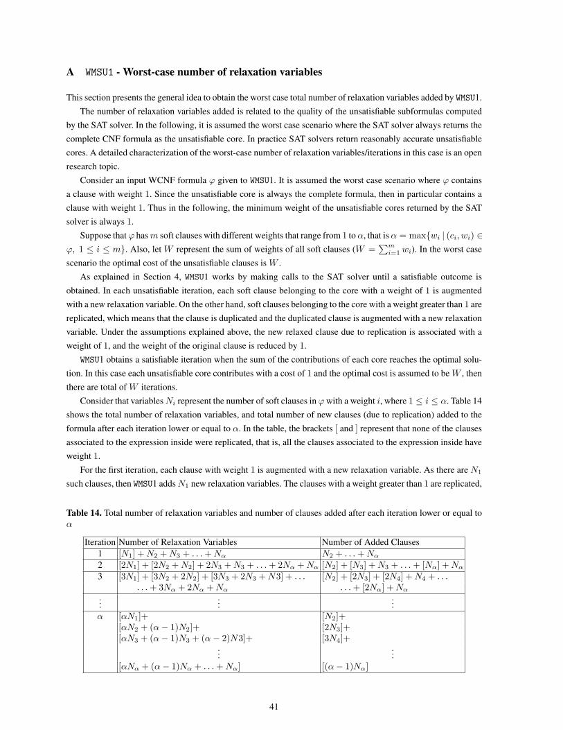
A WMSU1 - Worst-case number of relaxation variables

This section presents the general idea to obtain the worst case total number of relaxation variables added by WMSU1.

The number of relaxation variables added is related to the quality of the unsatisfiable subformulas computed

by the SAT solver. In the following, it is assumed the worst case scenario where the SAT solver always returns the

complete CNF formula as the unsatisfiable core. In practice SAT solvers return reasonably accurate unsatisfiable

cores. A detailed characterization of the worst-case number of relaxation variables/iterations in this case is an open

research topic.

Consider an input WCNF formula ϕ given to WMSU1. It is assumed the worst case scenario where ϕ contains

a clause with weight 1. Since the unsatisfiable core is always the complete formula, then in particular contains a

clause with weight 1. Thus in the following, the minimum weight of the unsatisfiable cores returned by the SAT

solver is always 1.

Suppose thatϕ hasm soft clauses with different weights that range from 1 toα, that isα = max{wi | (ci, wi) ∈

ϕ, 1 ≤ i ≤ m}. Also, let W represent the sum of weights of all soft clauses (W =∑m

i=1 wi). In the worst case

scenario the optimal cost of the unsatisfiable clauses is W .

As explained in Section 4, WMSU1 works by making calls to the SAT solver until a satisfiable outcome is

obtained. In each unsatisfiable iteration, each soft clause belonging to the core with a weight of 1 is augmented

with a new relaxation variable. On the other hand, soft clauses belonging to the core with a weight greater than 1 are

replicated, which means that the clause is duplicated and the duplicated clause is augmented with a new relaxation

variable. Under the assumptions explained above, the new relaxed clause due to replication is associated with a

weight of 1, and the weight of the original clause is reduced by 1.

WMSU1 obtains a satisfiable iteration when the sum of the contributions of each core reaches the optimal solu-

tion. In this case each unsatisfiable core contributes with a cost of 1 and the optimal cost is assumed to be W , then

there are total of W iterations.

Consider that variablesNi represent the number of soft clauses in ϕwith a weight i, where 1 ≤ i ≤ α. Table 14

shows the total number of relaxation variables, and total number of new clauses (due to replication) added to the

formula after each iteration lower or equal to α. In the table, the brackets [ and ] represent that none of the clauses

associated to the expression inside were replicated, that is, all the clauses associated to the expression inside have

weight 1.

For the first iteration, each clause with weight 1 is augmented with a new relaxation variable. As there are N1

such clauses, then WMSU1 addsN1 new relaxation variables. The clauses with a weight greater than 1 are replicated,

Table 14. Total number of relaxation variables and number of clauses added after each iteration lower or equal to

α

Iteration Number of Relaxation Variables Number of Added Clauses

1 [N1] +N2 +N3 + . . .+Nα N2 + . . .+Nα

2 [2N1] + [2N2 +N2] + 2N3 +N3 + . . .+ 2Nα +Nα [N2] + [N3] +N3 + . . .+ [Nα] +Nα

3 [3N1] + [3N2 + 2N2] + [3N3 + 2N3 +N3] + . . . [N2] + [2N3] + [2N4] +N4 + . . .

. . .+ 3Nα + 2Nα +Nα . . .+ [2Nα] +Nα

......

...

α [αN1]+ [N2]+[αN2 + (α− 1)N2]+ [2N3]+[αN3 + (α− 1)N3 + (α− 2)N3]+ [3N4]+

......

[αNα + (α− 1)Nα + . . .+Nα] [(α− 1)Nα]

41

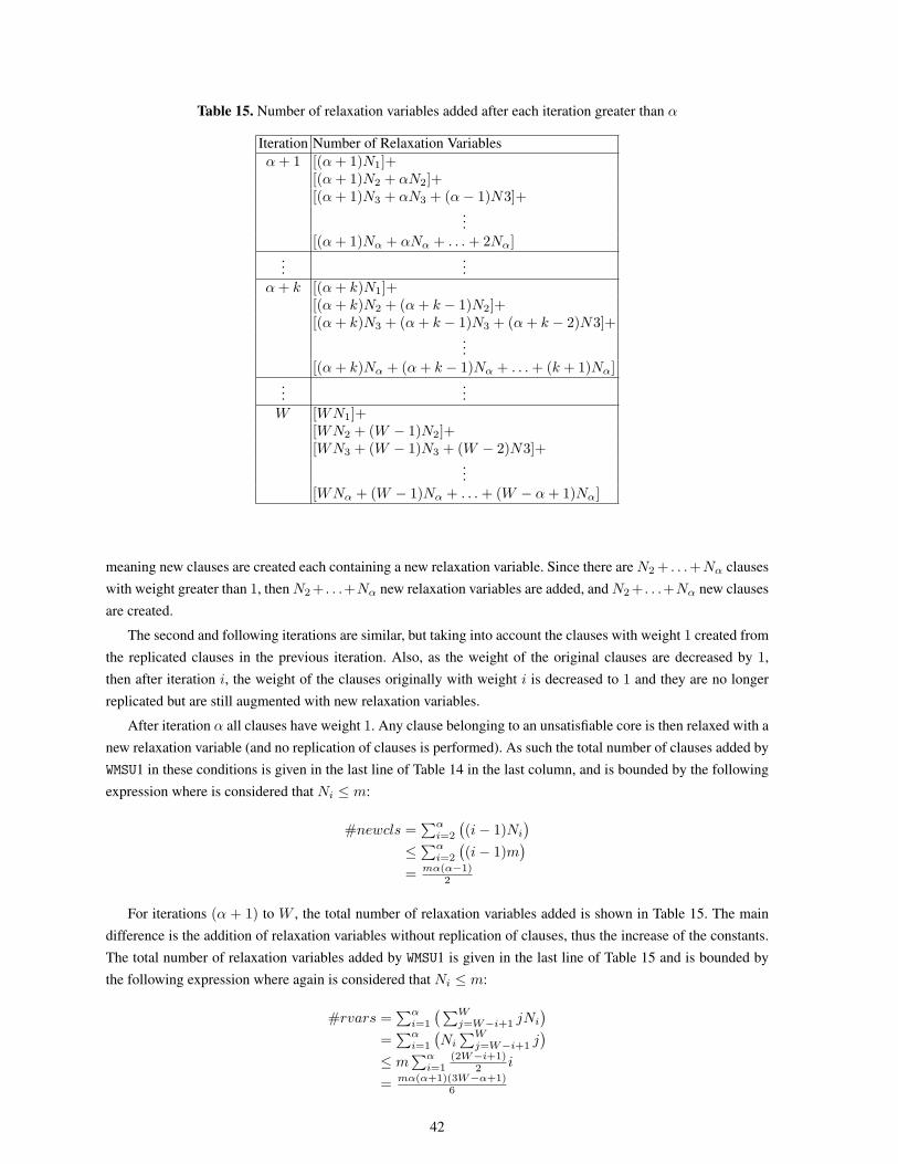
Table 15. Number of relaxation variables added after each iteration greater than α

Iteration Number of Relaxation Variables

α+ 1 [(α+ 1)N1]+[(α+ 1)N2 + αN2]+[(α+ 1)N3 + αN3 + (α− 1)N3]+

...

[(α+ 1)Nα + αNα + . . .+ 2Nα]...

...

α+ k [(α+ k)N1]+[(α+ k)N2 + (α+ k − 1)N2]+[(α+ k)N3 + (α+ k − 1)N3 + (α+ k − 2)N3]+

...

[(α+ k)Nα + (α+ k − 1)Nα + . . .+ (k + 1)Nα]...

...

W [WN1]+[WN2 + (W − 1)N2]+[WN3 + (W − 1)N3 + (W − 2)N3]+

...

[WNα + (W − 1)Nα + . . .+ (W − α+ 1)Nα]

meaning new clauses are created each containing a new relaxation variable. Since there are N2+ . . .+Nα clauses

with weight greater than 1, thenN2+ . . .+Nα new relaxation variables are added, andN2+ . . .+Nα new clauses

are created.

The second and following iterations are similar, but taking into account the clauses with weight 1 created from

the replicated clauses in the previous iteration. Also, as the weight of the original clauses are decreased by 1,

then after iteration i, the weight of the clauses originally with weight i is decreased to 1 and they are no longer

replicated but are still augmented with new relaxation variables.

After iteration α all clauses have weight 1. Any clause belonging to an unsatisfiable core is then relaxed with a

new relaxation variable (and no replication of clauses is performed). As such the total number of clauses added by

WMSU1 in these conditions is given in the last line of Table 14 in the last column, and is bounded by the following

expression where is considered that Ni ≤ m:

#newcls =∑α

i=2

(

(i− 1)Ni

)

≤∑α

i=2

(

(i− 1)m)

= mα(α−1)2

For iterations (α + 1) to W , the total number of relaxation variables added is shown in Table 15. The main

difference is the addition of relaxation variables without replication of clauses, thus the increase of the constants.

The total number of relaxation variables added by WMSU1 is given in the last line of Table 15 and is bounded by

the following expression where again is considered that Ni ≤ m:

#rvars =∑α

i=1

(∑W

j=W−i+1 jNi

)

=∑α

i=1

(

Ni

∑Wj=W−i+1 j

)

≤ m∑α

i=1(2W−i+1)

2 i

= mα(α+1)(3W−α+1)6

42

iterative and core-guided maxsat solving a survey...

Documents