CTT and IRT 1

Test Construction using CTT and IRT with Unrepresentative Samples

Alan D. Mead

Illinois Institute of Technology

Adam W. Meade

North Carolina State University

Running Head: CTT AND IRT

Alan D. Mead, College of Psychology, Illinois Institute of Technology; Adam W. Meade,

Department of Psychology, North Carolina State University. We wish to thank Scott Morris and

Mike Zickar, for insightful discussions about these topics, and Avi Fleischer, Aaron Miller and

Brendan Neuman, for their helpful comments on prior drafts. Correspondence concerning this

article should be addressed to Alan D. Mead, College of Psychology, Illinois Institute of

Technology, 3101 South Dearborn, Chicago, IL 60616. E-mail: mead@iit.edu

CTT and IRT 2

Abstract

We compare test construction using CTT and IRT in several sample sizes (from N=20 to

N=5000) and degrees of representativeness (represented by selecting the top 20%, 40%, 60%,

80% or 100% of a population) using a Monte-Carlo simulation design. Little support was found

for our hypothesis that IRT would outperform CTT in building informative tests, especially in

large or unrepresentative samples. The test construction algorithm was more influential than

sample size or representativeness; picking the most discriminating items from across the range of

difficulty slightly favored CTT, while IRT was slightly favored when the IRT test construction

algorithm directly maximized the evaluation criteria. We conclude that test construction using

either CTT or IRT produces empirically similar exams and IRT is only preferred when there is a

target test information function.

CTT and IRT 3

Test Construction using CTT and IRT with Unrepresentative Samples

Item response theory (IRT) has clearly gained “mindshare” among I/O psychologists and

researchers, as well as psychometricians. In part, this may be due to “advertising” about the

advantages of IRT over CTT. Over thirty years ago, Ben Wright wrote: “... you will find that

this small point (of sample dependency of classical measurement statistics) is a matter of life and

death to the science of measurement. The truth is that the so-called measurements that we now

make in educational testing are no damn good!” (Wright & Stone, 1978, p. ix). Almost twenty

years ago, Eason wrote “[m]easurement theory has advanced beyond classical test theory” (1991,

p. 97) and in 2000 Embretson and Reise wrote “[IRT] has rapidly become mainstream as the

theoretical basis for measurement” (p. 3). IRT has generated “new rules” of measurement

(Embretson & Hershberger, 1999) and is often cited as superior to CTT (Zickar & Broadfoot,

2010).

While the theoretical benefits of IRT are noteworthy, there is very little empirical

validation of the benefits of IRT over CTT under basic test construction scenarios. Among the

few studies conducted to date that compared IRT and CTT values, conclusions have been

somewhat conflicting. For instance, Lawson (1991) found CTT methods and the IRT Rasch

model to function almost identically. MacDonald and Paunonen (2001) partially replicated these

results but concluded that test construction is preferred with IRT. One reason why researchers

finding similar results may reach different conclusions is the choice of measure of test quality

(e.g., correlation between true and estimated item parameter). While such metrics are valuable,

these metrics are not directly actionable. Is a correlation of the true and estimated item

CTT and IRT 4

parameter slope of 0.482 sufficient for my needs? This question illustrates a shortcoming of the

traditional approach in the existing literature.

The primary goal of this study is to simulate an important psychometric application in

order to determine whether IRT or CTT works better for that application. By simulating an

application, we will produce more actionable and interpretable results than past research. The

application we chose was the construction of general-purpose tests (tests that do not have a cut-

score and which therefore require good precision across a wide range of scores). Our results add

to the empirical knowledge about the relative usefulness of CTT and IRT for a very important

psychometric process.

IRT and CTT

CTT. Classical test theory (CTT; Novick, 1966; Lord & Novick, 1968) is defined by

some simple, axiomatic assumptions:

X T E= + , (1)

where X is the observed test score, T is the latent true test score (T=E{X}, the expectation of X),

and a latent, stochastic error score, E. If T=E{X} then it follows that E{E}=0. We must also

assume that error scores are independent of any true or other error score:

( , ) 0E Tρ = (2)

( , ') 0E Eρ = (3)

Thus, CTT is less a model than a set of axioms; van der Linden and Hambleton (1997) say that

this model is “always true” in the sense that we do not test these axioms. Also, CTT is clearly

focused on total test score — not only in the obvious sense that the model considers only test

CTT and IRT 5

scores, because we might apply CTT to one-item tests and then it is a theory about item scores.

However, no manipulation of these axioms makes it a model of both item and test scores.

Although CTT does not address items per se, a range of item statistics have been

developed for test construction. The two most commonly-used are item difficulty and item

discrimination. Item difficulty is indexed by the proportion of individuals in a sample that

answer an item correctly, so values near zero indicate a hard item and values near 1.0 indicate an

easy item. Item discrimination is usually indexed by correlating the item scores with the total

test scores (the item-total correlation) or the test scores omitting the target item (the corrected

item-total correlation), though sometimes this term is used to describe differences in the item

difficulty for high and low performing respondents. Values of the item-total correlation at or

below zero indicate a poorly functioning item (strong negative correlations are a sign of a

miskeyed item).

Test scoring and construction using CTT is fairly straight-forward. The most common

test score for a test developed using CTT is the number (or percent) of items answered correctly.

From purely statistical considerations, test construction using CTT might often consist of

selecting those items with the best discrimination (item-total correlation) and which span a range

of item difficulties.

IRT. Item response theory (IRT) provides statistical models relating a latent trait to the

probability of responding to an item. A common IRT model for dichotomous items is the three-

parameter logistic (3PL):

1( 1| )1 exp( ( ))

ii j i

i j i

cP u ca b

θ θθ

−= = = ++ −

, (4)

CTT and IRT 6

where ui is the 0/1 item response, θj is the ability of an individual test-taker, ai is the slope of the

function (proportional to the factor loading of this item onto the latent trait), bi is the location

(interpreted as difficulty for ability items), and ci is the left asymptote (interpreted as the psuedo-

guessing level for multiple-choice ability items). The function defined in Eq. 4 is called the item

characteristic curve (ICC) or item response function (IRF). A two parameter (2PL) model is

obtained by assuming that ci = 0 (i.e., no guessing) and a one-parameter model is obtained by

setting ai = 1 (i.e., all items are equally related to the latent trait; the 1PL is almost identical to the

Rasch model, van der Linden & Hambleton, 1997).

Test construction using IRT might proceed from estimated item parameters or by

selecting items based on their information functions (described below) to match a target function.

In the former case, IRT test construction might look quite similar to CTT test construction. The

slope parameter, ai, is analogous to the item-total correlation and the difficulty parameter, bi, is

analogous to the CTT difficulty (Lord, 1980). In addition, test developers should avoid items

with large psuedo-guessing, ci, parameters. Tests developed using IRT can generally be scored

using number-correct. If desired, the “IRT score” can be calculated by estimating theta values

for each examinee ( ˆθ , theta-hat). Though these theta-hat scores typically correlate highly (e.g.,

> .95) with number correct (Embretson & Reise, 2000).

Measurement error. In CTT, measurement error is primarily indexed by the reliability

of a set of scores, ρXX':

2 2

' 2 21T EXX

X X

σ σρσ σ

= = − , (5)

CTT and IRT 7

where the σ2 terms are variances of the values from Eq. 1. Reliability is the degree to which an

observed measurement is due mainly to stochastic error (for low values) or relatively free from

error (for values approaching 1.0). Because the terms in Eq. 5 are unobservable, much of the

body of CTT theory and practice concerns estimating reliability and several methods are

available. Note that a single reliability is defined for all scores from any given sample. CTT

also provides an index of reliability that is expressed in a more meaningful metric, the standard

error of measurement (i.e., the standard error of X; SEM):

2'1X XXSEM σ ρ= − . (6)

The SEM is very useful in practice because, with the added assumption that the sampling

distribution of X is normal, we can construct confidence intervals around the observed test score,

X. As with the reliability, a single SEM value is provided for all scores.

Item response theory provides Fisher information for θ (theta, the person-parameter; i.e.,

the test-taker's standing on the latent trait) as a replacement for CTT reliability. Fisher

information indexes the degree of information available to estimate a statistical parameter. Items

provide more information about θ in regions of the score scale where the item response function

(IRF) is changing rapidly and little information to estimate θ in regions where the IRF is flat.

Thus, information is a function over levels of θ and depends upon the available item(s). A single

item has an information function, Ii(θ), defined as the ratio of the rate of change of the IRF over

the item variance:

2'

2( ) ii

i

PI θ

σ

= . (7)

CTT and IRT 8

A very useful IRT property is that individual item information functions sum to a test

information function, I(θ):

( ) ( )iI Iθ θ= ∑ . (8)

Thus, IRT is truly a theory about items as well as tests. IRT also defines an SEM as the

sampling standard error of θ, which is also a function of θ and reciprocal to the test information

function:

1ˆ( | )( )

SEI

θ θθ

= . (9)

Comparison of CTT and IRT. As described above, IRT provides a richer set of tools

for test developers. IRT provides a psuedo-guessing parameter that has no common analog in

CTT and IRT provides a means to assess degree of measurement equivalence at various points

on the score scale and based on different sets of items. Thus, the item analysis statistics provided

by both IRT and CTT are fairly comparable, but IRT provides an additional item characteristic

and a more sophisticated mechanism for conceptualizing measurement error.

As a statistical modeling approach, IRT has other advantages over CTT. For example,

while all CTT concepts are specific to a given sample, the parameters of an IRT model hold for

an entire population. That is, the parameters of an IRT model are said to be invariant to sub-

populations (i.e., samples). Perhaps subtle, an important advantage of IRT is the flexibility

afforded by the model. For example, different sets of items could be administered to individual

test-takers and yet comparable estimated theta can be estimated from these different tests.

Another advantage of IRT models is that they represent the ability of the test-takers and

the difficulty of the items as independent parameters. This is a significant issue because CTT

CTT and IRT 9

(wherein all values are sample-specific) has no way to separately identify these two constructs.

The same items will appear easy in a sample of high-ability test-takers and difficult in low-

ability samples. Thus, IRT can separate these two empirically intertwined concepts in a way that

no other psychometric approach can do.

Also, IRT lends itself to simulating data in a way that would be difficult using CTT. For

example, when planning a computer adaptive test (CAT) a psychometrician might wonder if the

item pool is sufficient. Using IRT, it is possible to simulate the CAT administration and

determine whether the psychometric properties of the CAT scores are sufficient (see Harwell,

Stone, Hsu, Kirisci, 1996).

While IRT does everything that CTT does and more, there are a few possible advantages

of CTT. One is practical; CTT is simple. Whereas IRT requires relatively obscure software,

CTT item analysis is easy to conduct in common statistical packages. Also, whereas CTT

statistics are easily computed, IRT statistics must be estimated, which is more complex in its

own right and requires a thorough model-data-fit analysis after estimation. Moreover, explaining

test properties to lay persons (e.g., job candidates that may ask about the test used for hiring) is

considerably more simple using CTT.

The other advantage of CTT is that it has few assumptions. The assumptions underlying

IRT models are chiefly that: (1) all items are completely caused by the latent trait and an item-

specific factor; and (2) that all item-specific factors are mutually independent (Lord, 1980). This

is essentially a confirmatory factor analysis model in which all items load on a single latent

variable and each item's uniquenesses are uncorrelated (McDonald, 1997). Therefore, CTT may

CTT and IRT 10

be a better choice for some situations in which IRT models do not fit well because of violations

of the assumptions or shape of the model.

One issue has not been the subject of much empirical research: it is known that

estimation of the parameters of an IRT model requires large samples (Hulin, Lissak, & Drasgow,

1982) but, of course, the means, variances and correlations computed under CTT would also

benefit from large samples. While a fair amount of research has examined the sample sizes

required for effective IRT estimation, very little research has directly compared the sample size

requirements of IRT and CTT. It is assumed that CTT would work better in smaller samples

(Zickar & Broadfoot, 2010; Ellis & Mead, 2002), but this has not been empirically studied.

In conclusion, IRT seems to be superior to CTT in many ways. It is conceptually

superior, IRT provides a richer selection of tools for test developers, and IRT has advantages that

are hard to quantify, like greater flexibility, invariance of the parameters, and providing “proper”

statistical models. The only area where the superiority of IRT is not obvious is for smaller

samples or tests which were not unidimensional (or where, for other reasons, the data do not fit

the IRT model), and perhaps in the area of “ease of use.”

Previous research. No previous research has compared IRT and CTT in the specific

application of scale construction, however three prior studies have compared these two methods.

These three studies are surprising in two ways. First, it is surprising that very few empirical

comparisons have been conducted. Also, the empirical comparisons have been surprisingly

mixed given the expected advantages of IRT.

Lawson (1991) compared Rasch model item- and person-parameters to CTT difficulty

and number-right in three sets of examination data. His CTT and IRT results were so similar that

CTT and IRT 11

he questioned whether there was any advantage to the additional work required to apply the

Rasch model. Lawson's findings may not be surprising given that the number right score is well

known as a sufficient statistic for theta in the Rasch model. The “sufficient statistic” relationship

between number right and theta does not necessarily imply a perfect linear correlation, but one

would be surprised to find anything but a high correlation. Also, the Rasch model is the simplest

IRT model; only item difficulty can influence the estimation of theta. In contrast, when using the

3PL model, the slope of the item and the psuedo-guessing parameter would also influence

estimation of theta. It is possible that the complexity of the IRT model influences the

comparability of IRT and CTT statistics, with the simpler Rasch model being closer to CTT and

more complex IRT models perhaps being quite different from CTT.

Fan (1998) examined the comparability of IRT and CTT statistics and test scores using

the 1PL, 2PL and 3PL IRT models. Because Fan used real data sets, no comparison between

true values and estimates could be made; rather he compared CTT and IRT results (e.g., the

correlation between IRT difficulty parameters and CTT proportion correct values). Fan found a

high degree of comparability between IRT theta-hat values and CTT NR values (the lowest

correlation was 0.966) with 2PL estimates slightly less comparable than those of the 1PL and

3PL models. The item difficulty statistics were also highly correlated. The correlations were

almost all 0.999 for the 1PL and were generally larger than 0.90. Again, the 2PL estimates were

slightly less comparable than the 3PL estimates. Item discrimination parameters differed most

from CTT item-total correlations with most correlations less than 0.90 and a few lower than 0.40

(note that the Rasch model estimates were not included in this analysis, because they had no

variance and could not co-vary).

CTT and IRT 12

Fan (1998) also compared CTT and IRT estimates from different subsamples of N=1000

to investigate the invariance properties of CTT and IRT parameter estimates. He created

samples varying in their representativeness by sampling a larger dataset (e.g., random selections

vs. men and women vs. high and low scores). Of course, IRT parameters are known to be

invariant but Fan was testing the empirical invariance of the IRT item parameter estimates and

comparing them to estimates of CTT statistics, which are thought not to be invariant. Fan found

that both CTT and IRT difficulty, and to a lesser degree, discrimination statistics displayed

invariance. For item difficulty, CTT estimates were closer to perfect invariance. In his

conclusion, Fan questioned whether IRT had the “advertised” advantages over CTT.

Taken together, Lawson's (1991) and Fan's (1998) results seem damning for IRT — at

least in terms of the inherent superiority generally afforded to IRT. However, Lawson's study

used only the Rasch model and Fan's comparison of the Rasch model with the 2PL and 3PL

suggests that the Rasch model may be least different from CTT. Neither Lawson's nor Fan's

study simulated the response data, so they were unable to compare the estimates to population

parameters. Further, their dependent measure (correlations of IRT and CTT estimates) is

actually difficult to interpret; for example, is a correlation of 0.80 sufficient reason to abandon a

preference and declare IRT and CTT equivalent? If 64% of the variability was shared in

common, what accounted for the remaining third of the variability?

MacDonald and Paunonen (2001) felt that prior research might be influenced by the fact

that they were real-data studies. In particular, these researchers were interested in the effects of

the specific items used in the study. They also wished to examine accuracy, which was not

possible in the previous, real-data studies. Therefore, they simulated data using 1PL and 2PL

CTT and IRT 13

IRT models and then computed IRT and CTT statistics from these values. They performed three

sets of correlations. First, they tested comparability of test scores, difficulty, and item

discrimination by correlating estimated IRT and CTT statistics; they found very high

comparability for test scores and difficulty and less comparability for item discrimination. Next,

they correlated values obtained from different samples to test invariance; they found exceptional

invariance with CTT exhibiting slightly closer to perfect invariance as compared to IRT. These

results replicate Fan (1998), although this test of invariance seems weak because the different

groups appeared to be randomly equivalent. Finally, the researchers correlated the estimated and

true statistics to examine accuracy; they found excellent accuracy for test scores and item

difficulties and IRT item discrimination but far lower accuracy for CTT item discrimination.

In summarizing their results, MacDonald and Paunonen (2001) emphasize the possibility

of selecting non-optimal items during test construction with CTT and the probability of superior

results using IRT. Item discrimination is a very important aspect of test construction using IRT

because item information (Eq. 8) depends upon the square of the slope of the IRF and thus item

discrimination is the main determinant of the item information, which is maximized when the

item discrimination is large.

Thus, to summarize the prior literature, all previous studies have used correlations as the

dependent, outcome variable. Lawson (1991), Fan (1998) and MacDonald (MacDonald &

Paunonen, 2001) obtained extremely similar results but Fan concluded that IRT may not have

many advantages over CTT for traditional tasks, like test construction, while MacDonald

emphasized the advantages of using IRT to construct tests.

CTT and IRT 14

None of these studies have considered the role of statistical estimation in the results or

incorporated measurement error inherent in the CTT or IRT framework. Because it is a mean,

the error associated with CTT item difficulty (estimated by proportion correct) is very simple to

calculate: 2 2

XX Nσ σ= . The error of IRT item difficulty is a vastly more complex issue tied

intimately to the maximum likelihood estimation of the IRT parameters (the sampling error is

calculated as the inverse of the appropriate diagonal elements of the Hessian matrix; see Lord,

1980; Baker & Kim, 2004). This estimate of standard error is only correct asymptotically and

only when maximum likelihood estimates (MLE's) have been calculated (by default, BILOG-

MG estimates IRT difficulty using MLE, discrimination and guessing parameters are estimated

using a Bayesian approach). Even if a suitable, robust estimate of the sampling error of IRT

difficulty were available, it would not be directly comparable to CTT difficulty unless the IRT

model perfectly fits the data because the IRT estimate is the sampling error of a statistical model

parameter and does not include any model misfit. So, it is very difficult to compare the error

inherent in CTT and IRT parameters. However, it seems plausible that statistical parameters

estimated as part of a fairly complex model may have large standard errors in small samples.

This is the basic reason behind admonitions to use “large samples” with IRT.

Present Study

The current study compared IRT and classical test theory (CTT) in a very basic and

important application discussed by authors of prior research — building an exam from a bank of

items, manipulating sample size and sample representativeness. The main research goal was to

produce guidance for practitioners on when to select IRT or CTT for item analysis and selection.

CTT and IRT 15

Like MacDonald and Paunonen (2001) we used a Monte-Carlo simulation design.

However, we used item parameters from an actual exam in order to maximize the

generalizability of this simulation research. To generate unrepresentative samples, we simulated

an organizational context in which incumbents were unrepresentative of the application

population to some degree due to direct range restriction, which we varied from none (SR=1.0)

to fairly extreme (SR=0.20). We then simulated these incumbents responding to a large pool

(n=150) of pilot items and we used both CTT and IRT to analyze the pilot data and selected a 50-

item exam from this pilot pool. Thus, representativeness was operationalized by the mean and

variability of the calibration sample used for IRT and CTT analysis. In the SR=1.0 condition,

this calibration sample represented the target, N(0,1) population while other conditions had

higher means and a reduced variability as compared to the target population.

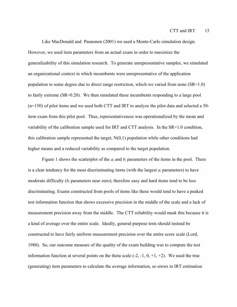
Figure 1 shows the scatterplot of the ai and bi parameters of the items in the pool. There

is a clear tendency for the most discriminating items (with the largest ai parameters) to have

moderate difficulty (bi parameters near zero); therefore easy and hard items tend to be less

discriminating. Exams constructed from pools of items like these would tend to have a peaked

test information function that shows excessive precision in the middle of the scale and a lack of

measurement precision away from the middle. The CTT reliability would mask this because it is

a kind of average over the entire scale. Ideally, general-purpose tests should instead be

constructed to have fairly uniform measurement precision over the entire score scale (Lord,

1980). So, our outcome measure of the quality of the exam building was to compute the test

information function at several points on the theta scale (-2, -1, 0, +1, +2). We used the true

(generating) item parameters to calculate the average information, so errors in IRT estimation

CTT and IRT 16

affected this outcome measure only through item choice. Also, by using the generating

parameters, we could compute the average test information for tests constructed using CTT. We

then computed the mean relative efficiency of the IRT and CTT tests:

( )( )

IRT

CTT

IRE Iθ

θ= . (10)

The choice of pool size (n=150) and exam length (n=50) was designed to be realistic and

yet to allow for capitalization on chance (Cureton, 1955). When fallible item statistics are

calculated and then the best items are chosen, invariably the random bias in the selected items is

towards more positive outcomes (e.g., higher item discrimination values). Regression to the

mean occurs when the selected set of items is evaluated independently. This effect plagues test

construction more when (1) there are many pilot items from which to select and (2) the item

statistics have larger sampling errors (e.g., in smaller samples). We felt that this choice of pool

size (n=150) and exam length (n=50) was ideal for comparing the goodness of exams

constructed using CTT and IRT.

Hypotheses. We find little to suggest in the previous research that IRT would be worse

than CTT and two prior studies compared item discrimination and found differences that might

advantage IRT. Therefore, our first hypothesis predicted that CTT would not out-perform IRT.

H1: Regarding choice of theory (IRT vs. CTT) for building exams, it was expected that IRT

would generally produce better results as compared to CTT (i.e., relative efficiencies above 1.0).

Some of our samples were highly unrepresentative (e.g., consisting of the top 20% of the

population). The invariance of the IRT model parameters to the estimation sample is frequently

cited as a major advantage of IRT (e.g., Wright & Stone, 1978; Embretson & Reise, 2000).

Previous research has suggested that invariance holds for both IRT and CTT person and item

CTT and IRT 17

parameters, however one simulation study found that the invariant CTT discrimination values

were inaccurate. Furthermore, Fan (1998) suggests that the scale of the CTT item difficulty

statistics is not interval (the tails are compressed), which we felt might lead to lower invariance

in extremely unrepresentative samples. Therefore, we expected that IRT would outperform CTT

in unrepresentative calibration samples.

H2: Exams built using IRT will outperform those built using CTT when unrepresentative

calibration samples have been used (relative efficiency will be greater than 1.0 in these

conditions).

The literature is silent on the issue of sample size. However, IRT is thought to require

large sample sizes for accurate parameter estimation and many assume that CTT will outperform

IRT in small samples.

H3: Exams built using CTT would outperform those built using IRT when calibration sample

size is small (relative efficiency will be less than 1.0 in these conditions).

What is a “small” sample in this context? We wondered whether there was a sample size,

such as N=200, under which we could clearly recommend that practitioners use CTT. This

question led to a research question:

RQ1: Is there a sample size, under which CTT should be preferred to IRT?

Method

Simulation. We simulated pilot test (e.g., calibration) samples of various sizes and

degrees of representativeness (i.e., the calibration sample represented the target, N(0,1)

population or had a mean higher and reduced variability as compared to the target population).

We created unrepresentative samples by modeling the situation in which a selection test was

CTT and IRT 18

developed using incumbents but used to select applicants. That is, we simulated incumbent

samples with direct range restriction using selection ratios of SR=0.2, 0.4, 0.6, 0.8, and 1.0. The

last level, SR=1.0 is a benchmark where the incumbent sample is completely representative of

the target population.

To adequately test our hypothesis and research question about sample size, we felt that

we needed to simulate conditions that spanned the range from extremely small to extremely

large. Therefore, we simulated samples of size N=20, 50, 100, 200, 500, 1000, and 5000.

Figure 2 shows the details of the simulation procedure. To generate a final sample of size

N after choosing the proportion SR, we first sampled N/SR theta values from a N(0,1)

distribution. To select these individuals, we simulated the administration of a 50-item selection

test (that test was composed of 50 additional items chosen randomly from the same bank; see

Appendix A1). We then selected the top N individuals to form the incumbent sample and

simulated these incumbent simulees completing the 150 items of the pool. ICL (Hanson, 2002)

was then used to fit IRT 3PL models to the items. Our simulation software calculated the CTT

item difficulty and corrected item-total point-biserial correlation. Using these CTT and IRT item

statistics, we built exams, computed the total information present in the exam using population

item parameters, and finally, we computed the mean relative efficiency for these exams.

Item bank. The item parameters shown in Appendix A1 were randomly sampled from a

larger bank of items used for adaptive administration of a well-known and widely-used exam.

As a condition of the use of the IRT estimates, the exam program required anonymity. The dual

purposes of the exam were certification and feedback, and thus the item pool should be

representative of pools used to create general purpose exams.

CTT and IRT 19

Exam construction. The exam construction algorithms are described in some detail in

Figure 3 and the complete Perl source code used to construct tests using CTT and IRT is shown

in Appendix A2. Initially, one exam construction algorithm (Algorithm 1) was implemented that

was parallel for CTT and IRT. We felt that by using a very similar exam construction algorithm,

the framework (CTT vs. IRT) would determine any differences. As described below, a second

IRT algorithm was introduced as “Algorithm 2”.

The CTT exam construction algorithm and the IRT Algorithm 1 were as parallel as

possible and involved two phases. In the first phase, the items were split into five difficulty

groups (called bins) and then the 10 “best” items within a difficulty group were selected (“best”

meant the items with the best CTT item-total correlation or IRT estimated item discrimination).

In this phase, the algorithm rejected items with very low item-total correlations or IRT

discrimination estimates. If this produced a complete 50-item test then the algorithm ended;

otherwise, the second phase simply selected the “best” remaining items (regardless of difficulty)

to make a 50-item form. Although this specific algorithm was devised for this study, it is

characteristic of the principles found in psychometric texts (Allen & Yen, 1979; Anastasi, 1988)

and thus of practice in this area. The choice of bins and other details are, of course, somewhat

arbitrary and were based upon the authors' expert judgment.

One could argue that Algorithm 1 is unfair to IRT because it ignores item and test

information, which are hallmarks of the IRT framework. Therefore, an IRT Algorithm 2 was

devised to leverage item information. This algorithm is comparatively very simple: mean item

information was calculated across the five target scale points for each item in the pool and the

best 50 items were chosen (here, “best” means items having the highest mean item information).

CTT and IRT 20

One could argue that this algorithm (Algorithm 2) favors IRT because it directly maximizes the

outcome measure.

A possibly important point: In all cases, the same data were analyzed in parallel by CTT

and IRT methods. The data for CTT and IRT are thus “paired-samples” rather than “independent

groups.” We felt that this approach minimized the effect of sampling error on the results.

Results

Table 1 summarizes our mean relative efficiency results over 40 to 50 replications. We

had planned (and ran) 50 replications in all cells, but ICL failed to converge in some instances.

We did not attempt to modify the ICL input to remedy this, nor did we replace these replications

(since by doing so, we might have modified the results). The difference in sampling error due to

having 40 or 50 replications is fairly small. The tabled values are IRT relative efficiencies (see

Eq., 10) computed from mean test information across five score points that span the useful range

of scores (θ = -2, -1, 0, +1, +2). Values of 1.0 indicate that the IRT and CTT forms had the same

mean level of information. Values above 1.0 favor IRT while values below 1.0 indicate that the

CTT exams had more information than those constructed using IRT. When calculating the test

information, we used the true (generating) item parameters so these values will not be inflated by

capitalization on chance.

In the top panel of Table 1, the initial results are shown (comparing CTT to the parallel

IRT Algorithm 1). Using what we felt was a parallel treatment of the CTT and IRT item

statistics to select the “best” items, the relative efficiencies are uniformly below 1.0, indicating

that the exams built using CTT uniformly outperformed those built using IRT Algorithm 1. In

the lower half of Table 1 are parallel results comparing the CTT method to IRT Algorithm 2,

CTT and IRT 21

which picked items to maximize the test information at five scale points. Using IRT Algorithm 2

the exams build using IRT performed as well or better than those constructed using CTT.

Hypothesis 1 was that exams constructed using IRT would perform as well or better than

exams constructed using CTT. In Table 1, both methods performed fairly similarly. The largest

value in the table (indicating the most advantage for IRT) was 1.09 while the smallest value

(indicating the most advantage for CTT) was .88, so no cell produced results where one method

was consistently far better than the other. Hypothesis 1 is supported for Algorithm 2 but not for

Algorithm 1.

Hypothesis 2 was that IRT would outperform CTT in building exams when samples were

unrepresentative. This hypothesis was not supported. In the top half of Table 1, CTT

outperforms IRT and in the bottom half of the table, the trend is for IRT to outperform CTT to

greater degrees as the samples became more representative. However, it is true that there was a

slight trend in the top half for IRT to be out-performed to a lesser degree in unrepresentative

samples.

Hypothesis 3 was that CTT would perform better in smaller samples. There appears to be

little support for this hypothesis. For Algorithm 1, CTT seems to gain slight advantages as

sample size increases. Probably, this simply reflects that, as samples become tiny, both CTT and

IRT perform increasingly poorly. In the bottom half of Table 1, no clear trend across columns is

visible. These results render our research question moot.

Discussion

IRT is becoming an increasingly popular psychometric framework but with little

empirical support for the advertised superiority. Our hypotheses concerned whether and when

CTT and IRT 22

IRT would support the construction of better (more uniformly informative) exams as compared

to CTT. None of our hypotheses were initially supported because our first exam construction

algorithm lead to better results for CTT. We interpreted this as evidence that CTT item statistics

extract the same information as IRT item statistics and CTT computational procedures are

(somewhat) more efficient than IRT estimation methods. If test construction is merely a matter

of picking the “best” items with a selection of difficulties, CTT may be a perfectly sufficient

methodology. We found little evidence of the problems with CTT test construction predicted by

MacDonald and Pounonen (2001).

We implemented Algorithm 1 to make item selection procedures across CTT and IRT

methods as parallel as possible. On the other hand, it could be argued that few researchers would

go through the effort of undertaking IRT analyses only to then disregarding the primary statistic

used in test construction, item information. One could argue that Algorithm 2 favors IRT

because it directly maximizes the evaluation criterion (i.e., IRT Algorithm 2 directly maximizes

information, which is used to compute mean relative efficiency). The results for Algorithm 2

were supportive of our Hypothesis 1.

Thus, our strongest result was that the specific algorithm used for test construction was

quite important. Simply picking the best items from across the range of difficulty worked fine

for CTT but IRT test construction worked best when the algorithm directly maximized the

evaluation criteria. However, overall these results mainly indicated that both CTT and IRT

produce approximately equally good exams and there is little reason to strongly prefer either

method on the basis of these fairly equal results.

CTT and IRT 23

We believe our present findings are quite consistent with the majority of previous

findings which suggested that CTT and IRT item statistics are quite comparable. The Algorithm

1 results that favored CTT could be seen as a refutation of the item discrimination issues raised

by MacDonald and Pounonen (2001). Taken together, the preponderance of evidence is that

CTT is an effective methodology for constructing tests. Some “advertised” benefits of IRT may

not be unique to IRT; both CTT and IRT produce approximately equivalently good exams for

samples varying substantially in their representativeness. However, IRT information can be used

to gain a slight advantage when there is a specific target information criterion.

Are our results due to metric issues? We have avoided discussing the relationship

between the fundamental indeterminacy of the metric of theta and the IRT population parameter

invariance. Theta has no natural metric and so one must be imposed. Therefore the numerical

values of invariant parameters can only be invariant up to a transformation. One might be

tempted to argue that we should transform the IRT parameter estimates for the unrepresentative

samples to the metric of the population. We believe that this is something of a red herring. First,

how would practitioners know what transformation to use? If we used information in our

simulation that was not available in actual practice, our results would not be generalizable, which

would be undesirable. Second, our CTT and IRT estimates suffer equally from whatever metric

issues arise from unrepresentative samples, so this issue should not have any effect on our

comparison of IRT and CTT. Indeed, this is the basis of H1 (predicting that IRT would be

superior to CTT). And finally, if we did transform both the IRT and CTT estimates, we doubt

that our results for IRT algorithm or sample size would be affected. If we did such (perhaps

artificial) transformations, we might erase the effects of unrepresentative samples.

CTT and IRT 24

In this study, and all previous studies, the CTT item-total correlation was the point-

biserial — that is the Pearson correlation uncorrected for the dichotomous nature of the item

score. The point-biserial correlation is known to under-estimate the true correlation when the

difficulty of the item is not .5 (Ellis & Mead, 2002). For extremely easy or difficult items, the

under-estimation might be substantial (McNemar, 1969). The solution to this problem is to use

the biserial correlation which “corrects” for the attenuation due to the dichotomization of the

item score. A careful reading of MacDonald and Pounonen (2001) suggests that CTT item

discrimination was least accurate when the items varied greatly in their difficulty. Our present

findings on the representativeness of the samples might be driven in part by greater attenuation

of the point-biserial item-total as the difficulty of the items became more extreme with less

representative samples. It would be interesting to see if the biserial correlation produces better

results. One reason why this is not a foregone conclusion is that the biserial involves additional

estimation.

The present results do not support the empirical superiority of IRT for constructing tests

except in the case where a specific target information function is desired. However, a specific

target information function does not cause IRT to produce substantially better results – CTT

simply lacks a mechanism to optimize a test information function. Thus, we believe that the

ultimate value of IRT is that it provides a richer “framework” to understand the functioning of

items and tests. Some psychometric problems may require this richer framework; for example, it

is hard to imagine computerized adaptive testing without IRT. In other cases, such as

constructing practically useful tests, IRT may not have substantial empirical or theoretical

advantages.

CTT and IRT 25

Limitations. In any simulation study, the generalizability of the results depends on the

similarity of the simulation parameters and conditions to an actual problem. We used items from

a real exam to maximize generalizability but the actual degree of generalizability will vary and

might be lower (and perhaps low) for some applications.

Regarding the outcome measure, it may be that including the evaluation points θ = -2 and

+2 was unrealistic as this corresponds to testing programs that measure from the third to the

ninety-seventh percentiles. But, of course, it is always the case that when there is a specific

measurement problem (e.g., setting a criterion on the 75TH percentile using such-and-such an

item pool), a simulation framed using the details of that problem will produce the best, most

specific answers.

Likewise, different design decisions might have affected the results we obtained. For

example, the choice of having a pool of 150 items from which to choose a 50-item exam

followed best practices (Nunnally & Bernstein, 1994) but may have provided more choice than is

available in some situations. In such cases, the exams created using IRT and CTT might be

expected to be similar simply because there are fewer choices. Also, the specific item

parameters of that pool might affect the outcome. As shown in Appendix A1, some of the items

were fairly poor items (the last five items in the pool all had IRT a parameters less than 0.20).

But none of the items had zero or negative item-total correlations, such as might be found in the

development of a new exam. Such “deviant” items can cause difficulty with convergence in IRT

parameters estimation (Lord, 1980), which could lead to worse results for IRT. On the other

hand, Sinar and Zickar (2002) found that IRT was better able to ignore deviant items.

CTT and IRT 26

The algorithms used in the present study were not rigorously optimized but differences

between Algorithms 1 and 2 produced the biggest effects in the study. It is possible that results

might be different for modified versions of our algorithms or alternative algorithms. For

example, algorithms that used more or fewer bins or an algorithm that transforms the CTT

difficulty to an interval scale before binning (see Fan, 1998, p. 363).

Summary and Advice for Practitioners. In summary, we compared IRT and CTT item

statistics in the task of test construction. Our primary outcome variable was the true mean test

information and results for both CTT and IRT were quite similar. Sample size and

representativeness had little effect on the relative performance of IRT and CTT. When we

simply picked items using CTT and IRT item discrimination values, exams built using CTT

slightly outperformed IRT. When we used a test construction algorithm that directly maximized

the criterion, exams built using IRT slightly outperformed those built using CTT. In particular,

we found no evidence that IRT was a better choice when samples were unrepresentative and we

found little evidence that CTT is a better choice when sample size is small.

Practitioners should not reflexively use IRT simply because of some “new rules” or

because some authority suggests that IRT has some superiority. In fact, in the absence of any

documented advantage for the task at hand, we would recommend that IRT be used when it is

necessary (e.g., when administering an exam adaptively) and that CTT should be used for all

other tasks.

CTT and IRT 27

References

Anastasi, A. (1988). Psychological testing (6th ed.). New York: Macmillan.

Baker, F. B., & Kim, S-H. (2004). Item response theory: Parameter estimation techniques

(Second edition). New York, NY: Marcel Dekker.

Chuah, S.C., Drasgow, F., & Luecht, R. (2006). How big is big enough? Sample size

requirements for cast item parameter estimation. Applied Measurement in Education,

19(3), 241-255.

Eason, S. (1991). Why generalizability theory yields better results than classical test theory: A

primer with concrete examples. In B. Thompson (Ed.), Advances in educational

research: Substantive findings, methodological developments (Vol. 1, pp. 83-98).

Greenwich, CT: JAI.

Ellis, B. B., & Mead, A. D. (2002). Item analysis: Theory and practice using classical and

modern test theory. In S. G. Rogelberg (Ed.), Handbook of research methods in

industrial and organizational psychology, (pp. 324-343). Malden, MA: Blackwell.

Embretson, S. E., & Hershberger, S. L. (1999). The new rules of measurement: What every

psychologist and educator should know. Mahwah, N.J.: L. Erlbaum Associates.

Embretson, S. E., & Reise, S. P. (2000). Item response theory for psychologists. Mahwah, NJ:

Lawrence Erlbaum.

Fan, X. (1998). Item response theory and classical test theory: an empirical comparison of their

item/person statistics. Educational and Psychological Measurement, 58(3), 357-381.

CTT and IRT 28

Harwell, M., Stone, C. A., Hsu, T. C.,& Kirisci, L. (1996). Monte Carlo studies in item response

theory. Applied Psychological Measurement, 20, 101-125.

Hanson, B. A. (2002). IRT Command Language. [Software manual]. Author.

Hulin, C. L., Lissak, R. I., & Drasgow, F. (1982). Recovery of two- and three-parameter logistic

item characteristic curves: A Monte Carlo study. Applied Psychological Measurement,

6(3), 249-260.

Lawson, S. (1991). One parameter latent trait measurement: Do the results justify the effort? In

B. Thompson (Ed.), Advances in educational research: Substantive findings,

methodological developments (Vol. 1, pp. 159-168). Greenwich, CT: JAI.

Lord, F. M. (1980). Applications of item response theory to practical testing problems.

Hillsdale, NJ: Erlbaum.

Lord, F. M., & Novick, M. R. (1968). Statistical theories of mental test scores. Addison-

Wesley, Reading, MA.

MacDonald, P., & Paunonen, S. V. (2001). A Monte Carlo comparison of item and person

statistics based on item response theory versus classical test theory. Educational and

Psychological Measurement, 62(6), 921-943.

McDonald, R. P. (1997). Normal-ogive multidimensional model. In W. J. van de Linden & R.

K. Hambleton (Eds.), Handbook of modern item response theory (pp. 258-270). New

York: Springer.

McNemar, Q. (1969). Psychological statistics (Fourth Edition). New York: Wiley.

Novick, M. R. (1966). The axioms and principal results of classical test theory. Journal of

Mathematical Psychology, 3(1), 1-18.

CTT and IRT 29

Nunnally, J. C., & Bernstein, I. H. (1994). Psychometric Theory (3RD Edition). New York,

NY: McGraw Hill.

Sinar, E.F., & Zickar, M.J. (2002). Evaluating the robustness of graded response model and

classical test theory parameter estimates to deviant items. Applied Psychological

Measurement, 26(2), 181-191.

van de Linden,W. J., & Hambleton, R. K. (1997). Item response theory: Brief history, common

models, and extensions. In W. J. van de Linden & R. K. Hambleton (Eds.), Handbook of

modern item response theory (pp. 1-28). New York: Springer.

Wright, B. D., & Stone, M. H. (1979). Best test design. Chicago: Mesa Press.

Zickar, M. J., & Broadfoot, A. A. (2009). The partial revival of a dead horse? Comparing

classical test theory and item response theory. In C. E. Lance and R. J. Vandenberg

(Eds.), Statistical and methodological myths and urban legends: Doctrine, verity and

fable in organizational and social sciences (pp. 37-60). New York, NY: Routledge.

CTT and IRT 30

Table 1.

Relative efficiency (IRT/CTT) of tests created using IRT and CTT

Selection Sample size Ratio 20 50 100 200 500 1000 2000 5000 Mean

Algorithm 1 (Pick best items).20 0.970 0.955 0.975 0.959 0.949 0.942 0.929 0.916 0.949.40 0.940 0.933 0.927 0.935 0.926 0.916 0.912 0.900 0.924.60 0.946 0.927 0.902 0.900 0.911 0.911 0.908 0.908 0.914.80 0.957 0.893 0.882 0.882 0.891 0.899 0.903 0.894 0.900

1.00 0.940 0.910 0.885 0.885 0.878 0.877 0.891 0.895 0.895Mean 0.951 0.924 0.914 0.912 0.911 0.909 0.909 0.903 0.916

Algorithm 2 (Maximize test information).20 1.002 1.008 1.016 1.001 1.000 1.003 0.998 0.993 1.003.40 1.009 1.003 0.998 0.993 0.993 0.991 0.996 0.996 0.997.60 1.019 1.008 0.997 1.001 1.004 1.011 1.018 1.024 1.010.80 1.038 1.021 1.030 1.028 1.052 1.065 1.070 1.072 1.047

1.00 1.049 1.056 1.069 1.069 1.072 1.083 1.089 1.091 1.072Mean 1.023 1.019 1.022 1.018 1.024 1.031 1.034 1.035 1.026

Note: Algorithms 1 and 2 are fully described in the text. Tabled values are relative efficiencies

(mean test information for forms created using IRT divided by mean test information for forms

created using CTT); values of 1.0 indicate no advantage; values below 1.0 favor CTT; and values

above 1.0 favor IRT. Based upon 40-50 replications.

CTT and IRT 31

Figure 1. IRT slope and difficulty parameters used to generate responses for the pretest pool.

CTT and IRT 32

Figure 2. Simulation procedure.

CTT and IRT 33

Figure 3. Exam construction algorithms

CTT exam construction• Divide the items into five bins (proportion correct thresholds: .60, .70, .80, .90)• Order the items within a bin by discrimination and select the top 10 items with corrected

item-total point-biserial correlations on 0.10 or better (or, if there are fewer than 10 such items in a bin, select all the items in a bin)

• If this produces fewer than 50 items (because some bins lacked enough items), then augment by ordering the remaining items by discrimination and selecting, top-down, sufficient items to make 50 items

IRT exam construction algorithm 1• Divide the items into five bins (IRT difficulty thresholds: -1.5, -0.5, +0.5, +1.5)• Order the items within a bin by discrimination and select the top 10 items with slope of

0.20 or greater (or, if there are fewer than 10 such items in a bin, select all the items in a bin)

• If this produces fewer than 50 items (because some bins lacked enough items), then augment by ordering the remaining items by discrimination and selecting, top-down, sufficient items to make 50 items

IRT exam construction algorithm 2• Loop through the pool of items and calculate the mean item information at θ = -2, -1, 0,

+1, +2; select the item with the highest mean information• Repeat the above step 49 more times

CTT and IRT 34

Appendix A1. Item parameters used in the pool.

Pool Items Selection ItemsItem a b c a b c

1 1.250 0.686 0.162 0.290 -3.091 0.2562 1.206 0.072 0.294 0.230 -2.383 0.2343 1.175 2.055 0.304 0.238 -2.189 0.2594 1.083 0.297 0.286 0.664 -1.618 0.1895 1.020 0.190 0.376 0.372 -1.563 0.0806 1.018 1.475 0.137 0.804 -0.558 0.4437 0.985 -0.205 0.157 0.737 -0.542 0.4178 0.982 2.079 0.166 0.338 -0.418 0.2819 0.979 0.595 0.137 0.560 -0.404 0.07810 0.956 1.717 0.297 0.660 -0.391 0.22211 0.932 0.906 0.327 0.188 -0.388 0.30212 0.927 -0.570 0.156 0.274 -0.371 0.13213 0.912 0.486 0.304 0.434 -0.230 0.24714 0.886 0.804 0.024 0.366 -0.209 0.35815 0.885 -0.014 0.091 0.855 -0.194 0.19916 0.859 0.531 0.254 0.597 -0.096 0.41017 0.825 0.251 0.285 0.578 -0.094 0.37118 0.819 0.470 0.237 0.765 -0.036 0.25219 0.816 0.885 0.180 0.833 0.028 0.27520 0.814 -0.784 0.225 0.922 0.073 0.19521 0.810 -0.737 0.126 0.844 0.096 0.33922 0.809 0.377 0.224 0.444 0.138 0.25323 0.804 -0.558 0.443 0.841 0.180 0.21324 0.799 2.750 0.146 1.083 0.297 0.28625 0.794 0.501 0.350 1.213 0.436 0.14426 0.794 -0.102 0.195 0.707 0.457 0.24327 0.787 2.110 0.076 0.638 0.538 0.18128 0.783 1.535 0.147 0.736 0.538 0.28729 0.765 -0.036 0.252 0.823 0.544 0.22030 0.763 -0.006 0.189 0.842 0.548 0.13431 0.762 1.324 0.097 0.396 0.625 0.11832 0.755 -0.065 0.263 0.232 0.632 0.35833 0.748 2.358 0.246 0.888 0.648 0.20334 0.734 0.510 0.282 0.630 0.650 0.26635 0.729 0.475 0.192 0.784 0.700 0.47836 0.726 0.928 0.272 0.596 0.707 0.26837 0.726 1.238 0.398 1.036 0.778 0.24838 0.724 0.060 0.125 0.351 0.786 0.25739 0.720 0.773 0.500 1.083 0.844 0.46740 0.715 -0.449 0.365 0.376 0.912 0.263

CTT and IRT 35

41 0.707 -0.595 0.103 0.622 0.923 0.11742 0.695 -0.613 0.143 0.659 0.986 0.16543 0.692 -0.009 0.500 0.589 1.128 0.49344 0.691 1.591 0.113 0.360 1.294 0.04545 0.684 3.121 0.131 0.845 1.333 0.39546 0.684 0.070 0.118 0.330 1.644 0.25847 0.682 0.922 0.164 0.982 1.763 0.05248 0.673 0.319 0.267 0.623 1.777 0.28449 0.667 1.131 0.292 0.320 1.948 0.42450 0.667 -0.148 0.118 0.745 3.964 0.07451 0.659 0.986 0.16552 0.644 1.905 0.18253 0.642 0.950 0.37354 0.642 -0.142 0.03955 0.641 -0.402 0.21056 0.639 -1.570 0.08157 0.638 0.468 0.17358 0.633 1.098 0.38059 0.627 2.596 0.26160 0.623 0.176 0.33261 0.610 -0.904 0.23462 0.608 0.479 0.23063 0.605 1.403 0.42164 0.603 -0.419 0.40865 0.599 1.418 0.22866 0.597 -0.096 0.41067 0.594 -0.378 0.10468 0.593 0.073 0.30069 0.586 0.253 0.43470 0.580 0.134 0.14871 0.577 0.200 0.19072 0.574 0.510 0.09973 0.569 1.188 0.03174 0.566 1.304 0.16975 0.560 0.658 0.19776 0.558 -2.086 0.24277 0.554 0.139 0.16678 0.550 -1.044 0.05279 0.540 0.921 0.18780 0.538 -1.289 0.14081 0.533 -0.800 0.21582 0.528 1.837 0.26683 0.519 0.163 0.30784 0.510 1.479 0.336

CTT and IRT 36

85 0.506 -1.256 0.22686 0.504 1.764 0.27287 0.497 1.748 0.45388 0.492 -0.344 0.31989 0.487 -0.219 0.03090 0.486 -0.916 0.13491 0.482 1.311 0.30692 0.469 1.115 0.06093 0.467 1.275 0.30394 0.464 2.055 0.34195 0.460 -1.215 0.23896 0.452 0.137 0.28597 0.451 -1.322 0.07898 0.445 0.863 0.50099 0.440 -1.098 0.346100 0.439 1.093 0.081101 0.435 1.580 0.274102 0.433 1.613 0.141103 0.427 1.799 0.113104 0.426 -0.603 0.335105 0.420 1.118 0.190106 0.418 0.295 0.050107 0.418 -0.783 0.134108 0.416 -0.335 0.329109 0.399 0.538 0.219110 0.396 0.625 0.118111 0.396 -0.550 0.247112 0.395 -2.466 0.305113 0.390 -1.411 0.290114 0.387 -1.045 0.171115 0.387 2.030 0.261116 0.378 -1.144 0.266117 0.377 -0.099 0.199118 0.375 0.039 0.246119 0.363 1.378 0.233120 0.357 0.343 0.210121 0.352 -1.737 0.063122 0.351 0.786 0.257123 0.350 -1.402 0.256124 0.350 -0.175 0.125125 0.335 -0.875 0.060126 0.330 1.644 0.258127 0.327 0.246 0.298128 0.327 -2.181 0.254

CTT and IRT 37

129 0.327 -1.231 0.307130 0.326 2.409 0.248131 0.325 -1.532 0.269132 0.305 -0.112 0.298133 0.294 -1.521 0.280134 0.285 0.513 0.260135 0.281 -2.471 0.213136 0.275 -0.570 0.223137 0.253 1.656 0.088138 0.249 0.718 0.126139 0.243 -3.175 0.268140 0.238 -2.189 0.259141 0.218 -1.066 0.156142 0.217 -0.302 0.308143 0.215 -0.562 0.158144 0.214 1.420 0.207145 0.204 1.603 0.249146 0.190 -1.585 0.299147 0.178 -2.915 0.234148 0.157 -5.209 0.274149 0.157 4.584 0.204150 0.144 -2.123 0.273

CTT and IRT 38

Appendix A2. Perl source code used to build CTT and IRT exams

# build_ctt_test - automatically build a test using CTT results# -------------------------------------------------------------sub build_ctt_test { my( $stats ) = @_;

my %used = (); my $CIT_MIN = 0.10; # avoid correlations below this

# break proportion correct into bins my @bl = qw/0.0 0.60 0.70 0.80 0.90/; # lower limit my @bu = qw/0.60 0.70 0.80 0.90 1.0/; # upper limit

# loop through bins; for each bin, pick the 10 # items with the best item-total (above a cut-off # minimum value) my $nbins = @bl; foreach my $bin ( 0..$nbins-1 ) {

# record the viable items my %temp = (); foreach my $s ( @$stats ) { if( $$s{pc} >= $bl[$bin] && # pc above LL $$s{pc} <= $bu[$bin] && # pc below UL !$used{ $$s{name} } && # item not used $$s{r} >= $CIT_MIN ) { # r is high enough $temp{ $$s{name} } = $$s{r}; # POSSIBLY use this } }

# pick the best of these, mark them as used my $count = 0; foreach my $item ( sort{ $temp{$b} <=> $temp{$a} } keys %temp ) { $count++; last if( $count > 10 ); $used{$item}++; } }

# do we have enough, or do we need to augment? if( scalar keys %used < 50 ) { print "Needed to augment!\n"; my %temp = map{ $$_{name} => $$_{r} } @$stats; my $count = scalar keys %used; foreach my $item ( sort { $temp{$b} <=> $temp{$a} } keys %temp ) { next if ( $used{ $item } ); $used{ $item }++; $count++; last if ( $count >= 50 ); } }

return [ sort { $a <=> $b } keys %used ];}

# build_irt_test1 - automatically build a test using IRT results# Algorithm 1: Similar to the CTT algorithm, bin items and select# the items with the highest slope within a bin; if needed, select

CTT and IRT 39

# remaining items from unused items with best slopes# -------------------------------------------------------------sub build_irt_test1 { my( $stats ) = @_;

my %used = (); my $MIN = 0.20; # avoid slopes below this

# define the "bins" where we will draw items my @bl = qw/-2.5 -1.5 -0.5 0.5 1.5/; # lower limit my @bu = qw/-1.5 -0.5 0.5 1.5 2.5/; # upper limit

# loop through bins; for each bin, pick the 10 items with # the best slope (avoiding those below a minimum value)

my $nbins = scalar @bl; # determine number of bins

# loop over the bins (the bins are numbered 0,1,2,...) foreach my $bin ( 0..$nbins-1 ) {

# record the viable items in %temp # %temp will hold pairs: temp{<item ID>} = <slope> my %temp = ();

# loop over all items foreach my $s ( @$stats ) { if( $$s{b} >= $bl[$bin] && # b above LL $$s{b} <= $bu[$bin] && # b below UL !$used{ $$s{name} } && # item not used $$s{a} >= $MIN ) # slope is high enough { $temp{ $$s{name} } = $$s{a}; # record in %temp for POSSIBLE use } }

# pick the 10 best of these items, mark them as used my $count = 0; # initialize counter to zero # below, we loop over the items in this bin; %temp is sorted # by slopes in decending order and we mark the top 10 as "used" foreach my $item ( sort{ $temp{$b} <=> $temp{$a} } keys %temp ) { $used{$item}++; # record this item as used print "IRT: using item $item in bin $bin with slope=$temp{$item}\n"; $count++; # increment number of items used last if( $count >= 10 ); # end loop if we have enough }

}

# do we have enough, or do we need to augment? if( scalar keys %used < 50 ) { print "Needed to augment!\n"; my %temp = map{ $$_{name} => $$_{a} } @$stats; # create %temp w/o restrictions my $count = scalar keys %used; # initialize count to our current number

# loop over all the items, sorted in decreasing order of slope foreach my $item ( sort { $temp{$b} <=> $temp{$a} } keys %temp ) { next if ( $used{ $item } ); # skip used items print "IRT: augmenting with item $item slope=$temp{$item}\n"; $used{ $item }++; # record this item as being used $count++; # increment our count

CTT and IRT 40

last if ( $count >= 50 ); # end loop when we have 50 items }

}

# return selected item ID's as a sorted list return [ sort { $a <=> $b } keys %used ];

}

# build_irt_test2 - automatically build a test using IRT information# Algorithm 2: Maximize the average info across a set of theta values# by iteratively picking the items that maximize this criterion# -------------------------------------------------------------sub build_irt_test2 { my( $stats, $thetas ) = @_;

# repeat, until we have 50 items... my %used = (); while( scalar keys %used < 50 ) {

# look thru all items for maximum information contribution my $max_info = 0; my $max_name = ''; foreach my $s ( @$stats ) {

next if( $used{ $$s{name}} ); # skip items already included

## calculate information for this item...

# loop over theta points my $count = 0; my $info = 0; foreach my $th ( @$thetas ) { $info += info3pl( $$s{a}, $$s{b}, $$s{c}, $th ); $count++; } $info = $info / $count; # compute average

# found a nex maximum? If so, note it if( $info > $max_info ) { $max_info = $info; # note the new maximum $max_name = $$s{name}; # note the associated item ID }

}

# now we know what item maximizes the IRT contribution $used{ $max_name }++;

}

return [ sort { $a <=> $b } keys %used ];

}