Open Access. © 2019 I. Ecsedi and Á. J. Lengyel, published by De Gruyter. This work is licensed under the Creative CommonsAttribution 4.0 License

Curved and Layer. Struct. 2019; 6:105–116

Research Article

István Ecsedi and Ákos József Lengyel*

An analytical solution for static problems ofcurved composite beamshttps://doi.org/10.1515/cls-2019-0009Received Nov 08, 2018; accepted Dec 27, 2018

Abstract: An analytical solution is presented for the deter-mination of deformation of curved composite beams. Eachcross-section is assumed to be symmetrical and the ap-plied loads are acted in the plane of symmetry of curvedbeam. In-plane deformations are considered of compositecurved beams. Assumed form of the displacement field as-sures the fulfillment of the classical Bernoulli-Euler beamtheory. The curvature of beam is constant and the internalforces in a cross-section is replaced by an equivalent force-couple system at the origin of the cylindrical coordinatesystem used. The internal forces are expressed in terms oftwo kinematical variables, which are the radial displace-ment and the rotation of the cross-sections. The determi-nation of the analytical solutions of the considered staticproblems are based on the fundamental solutions. Linearcombination of the fundamental solutions which are fill-ing to the given loading and boundary conditions, givesthe total solution. Closed form formulae are derived for theradial displacement, cross-sectional rotation, nomral andshear forces and bending moments. The circumferentialand radial normal stresses and shear stresses are obtainedby the integration of equilibrium equations. Examples il-lustrate the developed method.

Keywords: Analytical solution; curved composite beam;in-plane deformation; fundamental solution

1 IntroductionThe analysis of curved beam has been a topic of interest toresearch workers for over a century, it is a standard chap-ter in themost text-books ofmechanics of solids [1–7]. This

István Ecsedi: Institute of Applied Mechanics, University ofMiskolc, Miskolc-Egyetemváros, H-3515 Miskolc, Hungary; Email:mechecs@uni-miskolc.hu*Corresponding Author: Ákos József Lengyel: Institute of AppliedMechanics, University of Miskolc, Miskolc-Egyetemváros, H-3515Miskolc, Hungary; Email: mechlen@uni-miskolc.hu

topic is still concern at the present time because curvedbeam elements of constant curvature are important com-ponents in many modern engineering structures. In thispaper an analytical solution is presented for the solutionof statical boundary value problems of non-homogeneouscurved beams with constant curvature. For the solutionstatic bending problems of layered curved beams Seguraand Armengaud gave an analytical method [8]. Elastic-ity solutions are presented in [9] for curved beams withorthotropic functionally graded layers by means of Airystress functions. The developed method is illustrated incurved cantilever beams with different types of loadingconditions. Paper by Pydah and Sabale [10] presents andanalytical model for the flexure of bidirectional function-ally graded circular beam based on the Euler-Bernoullibeam theory. The material properties are simultaneouslysmooth functions of the polar angle φ and the radial coor-dinate r. The governing equations are solved for staticallydeterminate circular cantilever beams under the actionof tip loads. Static problems of curved composite beamswere analysed by finite element methods in the papers ofIbrahimbegović and Frey [11], Ascione and Fraternali [12]and Bhimaraddi et al. [13]. Paper by Dorfi and Busby [14]presents a laminated curved beam finite element with sixdisplacement degrees of freedom and three stress parame-ters. The classical lamination theory and the Timoshenkotheory are used to formulate the finite element. In [15] anew highly accurate composite laminated hybrid-mixedcurved beam element is presented by Kim. The formula-tion of thefinite element is basedon theHellinger-Reissnervariational principle and the first-order shear deformationtheory. Paper [16] presents a simple one-dimensional me-chanical model to analyse the static and dynamic featuresof non-homogeneous curved beams. The formulation ofthe analytical solution developed in this paper is basedon paper [16]. In the present paper according to [16] thefield equations and boundary conditions are formulatedin cylindrical coordinate system Orφz and it is assumedthat the plane z = 0 is the plane of symmetry includingthe material and geometrical properties and loading con-ditions. Thematerial and geometrical properties do not de-pend on polar angle φ, moduli of elasticity may depend

106 | I. Ecsedi and Á. J. Lengyel

on the cross-sectional coordinates (r, z), the curved beamin circumferential direction is homogeneous. This type ofnon-homogeneous curved beam is called φ-homogeneouscurved beam [16]. The definition of φ-homogeneity in-cludes those cases when the curved beam is a compositeof differentmaterials, so thatmoduli of elasticity are piece-wise constants. Type of these beams are laminated andfibre reinforced beams. Their discontinuities in materialproperties should not affect the presented analysis. Itmustbe mentioned that papers by Ecsedi and Lengyel [17, 18]provide analytical solution for layered curved compositebeams with interlayer slip. In paper [17] the deformationof curved composite beamwith partial shear interaction isdetermined under the action of concentrated radial load.Paper [18] gives numerical solution for in-plane deforma-tion of two-layer composite beam with flexible shear con-nection by the application of principle of minimum of po-tential energy.

In this study φ-homogeneous curved beams are con-sidered. Our aim is to develop an analytical solution todetermine the deflection, cross-sectional rotation, inter-nal forces and stresses. The presented method is based onthe fundamental solutions. The fundamental solutions ful-fil all the field equations and their initial values are zeroexcept only one of them. Linear combination of the fun-damental solutions which are fitted to given loading andboundary conditions provides the total solution of the con-sidered static equilibrium problem.

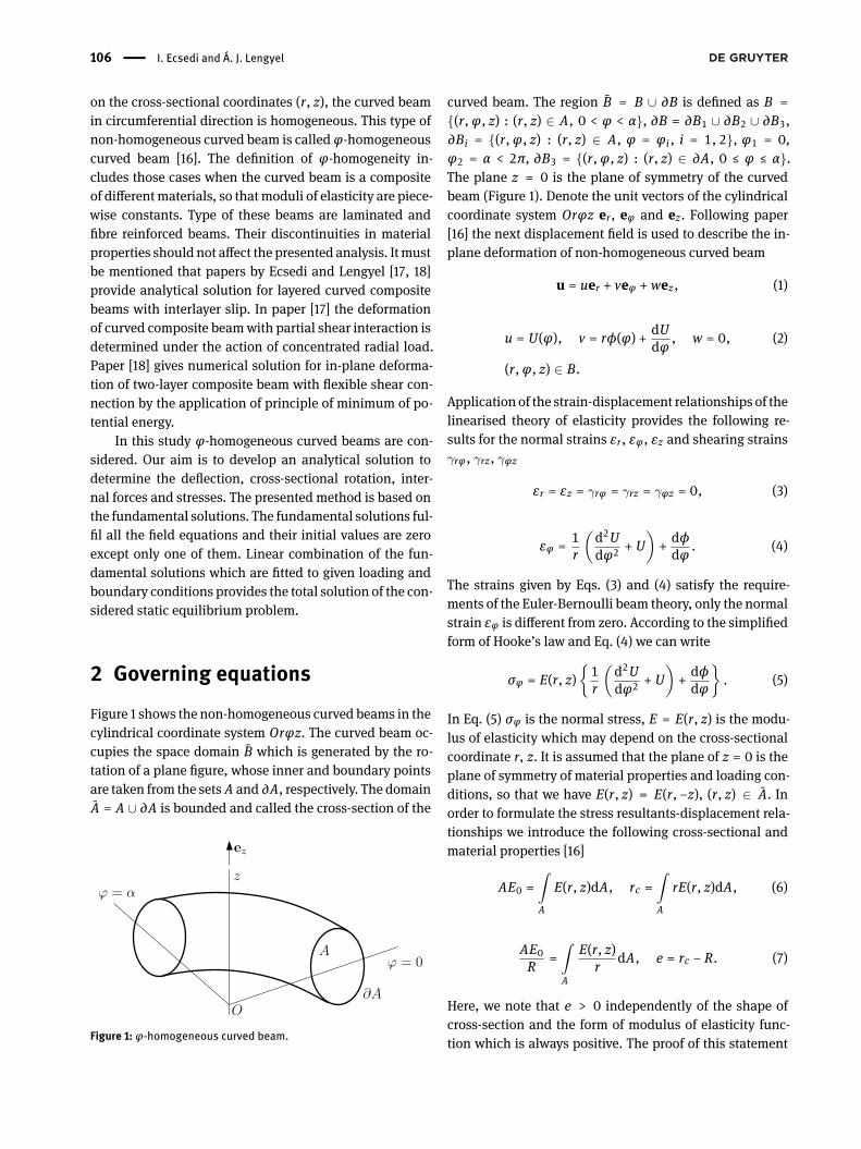
2 Governing equationsFigure 1 shows the non-homogeneous curved beams in thecylindrical coordinate system Orφz. The curved beam oc-cupies the space domain B which is generated by the ro-tation of a plane figure, whose inner and boundary pointsare taken from the sets A and ∂A, respectively. The domainA = A ∪ ∂A is bounded and called the cross-section of the

ϕ = 0

O

z

ez

A

∂A

ϕ = α

Figure 1: φ-homogeneous curved beam.

curved beam. The region B = B ∪ ∂B is defined as B ={(r, φ, z) : (r, z) ∈ A, 0 < φ < α}, ∂B = ∂B1 ∪ ∂B2 ∪ ∂B3,∂Bi = {(r, φ, z) : (r, z) ∈ A, φ = φi , i = 1, 2}, φ1 = 0,φ2 = α < 2π, ∂B3 = {(r, φ, z) : (r, z) ∈ ∂A, 0 ≤ φ ≤ α}.The plane z = 0 is the plane of symmetry of the curvedbeam (Figure 1). Denote the unit vectors of the cylindricalcoordinate system Orφz er, eφ and ez. Following paper[16] the next displacement field is used to describe the in-plane deformation of non-homogeneous curved beam

u = uer + veφ + wez , (1)

u = U(φ), v = rϕ(φ) + dUdφ , w = 0, (2)

(r, φ, z) ∈ B.

Application of the strain-displacement relationships of thelinearised theory of elasticity provides the following re-sults for the normal strains εr, εφ, εz and shearing strains𝛾rφ, 𝛾rz, 𝛾φz

εr = εz = 𝛾rφ = 𝛾rz = 𝛾φz = 0, (3)

εφ = 1r

(d2Udφ2 + U

)+ dϕdφ . (4)

The strains given by Eqs. (3) and (4) satisfy the require-ments of the Euler-Bernoulli beam theory, only the normalstrain εφ is different from zero. According to the simplifiedform of Hooke’s law and Eq. (4) we can write

σφ = E(r, z){1r

(d2Udφ2 + U

)+ dϕdφ

}. (5)

In Eq. (5) σφ is the normal stress, E = E(r, z) is the modu-lus of elasticity which may depend on the cross-sectionalcoordinate r, z. It is assumed that the plane of z = 0 is theplane of symmetry of material properties and loading con-ditions, so that we have E(r, z) = E(r, −z), (r, z) ∈ A. Inorder to formulate the stress resultants-displacement rela-tionships we introduce the following cross-sectional andmaterial properties [16]

AE0 =∫A

E(r, z)dA, rc =∫A

rE(r, z)dA, (6)

AE0R =

∫A

E(r, z)r dA, e = rc − R. (7)

Here, we note that e > 0 independently of the shape ofcross-section and the form of modulus of elasticity func-tion which is always positive. The proof of this statement

An analytical solution for static problems of curved composite beams | 107

follows from the next Schwarz’s inequality∫A

E(r, z)(√r)2dA

∫A

E(r, z)(√r)2

dA ≥ (8)

⎛⎝∫A

E(r, z)√r√rdA

⎞⎠2

.

The stress resultants are defined according to paper [16](Figure 2)

O

N(ϕ)S(ϕ)

M(ϕ)

ϕ

σϕ

ϕ = 0

A

Figure 2: Illustration of stress resultants and couple stress resul-tant.

N(φ) =∫A

σφdA, S(φ) =∫A

τrφdA, M(φ) (9)

=∫A

rσφdA.

In Eq. (9) τrφ = τrφ(r, φ, z) is the shearing stress, N isthe normal force, S is the shear force and M is the bend-ing moment. We note, in the Euler-Bernoulli beam theorythe shear force dos not effect to the deformation of non-homogeneous curved beam, its value is obtained by theapplication of the force equilibriumequation. Substitutionof (5) into Eqs. (8)1,3 gives

N(φ) = AE0(WR + dϕ

dφ

), (10)

M(φ) = AE0(W + rc

dϕdφ

).

Here, we introduce the designation

W(φ) = d2Udφ2 + U . (11)

In paper [16] the next equations of equilibrium are derived

∂N∂φ + S + fφ = 0, ∂S

∂φ − N + fr = 0, 0 < φ < α, (12)

∂M∂φ + m = 0. (13)

In Eqs. (12), (13) fr = fr(φ) and fφ = fφ(φ) are the appliedexternal forces and m = m(φ) is the applied moment ob-tained from the applied external forces [16]. Let V = V(φ)be defined as

V = dUdφ . (14)

Figure 3 enumerates some possible boundary conditions.

a) b)

c) d)

A

O

OA = R

e) f)

g)

O

F2

F1

M1

Figure 3: In plane boundary conditions for φ-homogeneous curvedbeams: a) Clamped end: U = 0, V = 0, ϕ = 0. b) Free end: N = 0,S = 0, M = 0. c) Simply supported in radial direction: U = 0,M = 0, N = 0. d) Pinned end: U = 0, rAϕ + V = 0, M − rAN = 0.e) Clamped-circumferentially guided end: U = 0, ϕ = 0, N = 0. f)Clamped-radially guided end: V = 0, ϕ = 0, S = 0. g) Loaded endcross section: N = F1, S = F2, M = M1.

108 | I. Ecsedi and Á. J. Lengyel

3 Equations of state of stressesThe cross-section A of the φ-homogeneous curved beamcan be represented in terms of thickness function t = t(r)(Figure 4) as

A = {(r, z) : |z| ≤ 0.5t(r), r1 ≤ r ≤ r2}, (15)r1 = min

(r,z)∈Ar, r2 = max

(r,z)∈Ar.

r

r 2

r 1

O z

t(r)

r

Figure 4: Illustration of r1 and r2.

We introduce the new type of stress resultants, i.e. stressesintegrated through the thickness, which are

nφ(r, φ) =0.5t(r)∫

−0.5t(r)

σφ(r, φ, z)dz, (16)

nr(r, φ) =0.5t(r)∫

−0.5t(r)

σr(r, φ, z)dz, (17)

nrφ(r, φ) =0.5t(r)∫

−0.5t(r)

τrφ(r, φ, z)dz. (18)

Equation of mechanical equilibrium in terms of thesestress resultants can formulated as

∂∂r

(r2nrφ

)+ r ∂nφ∂φ = 0, (19)

∂∂r (rnr) − nφ +

∂nrφ∂φ = 0.

Assuming that only the radial normal stress act at r = r2then we have the next stress boundary conditions

nrφ(r1, φ) = nrφ(r2, φ) = 0, (20)

nr(r1, φ) = 0, nr(r2, φ) =fr(r2, φ)r2

.

From Eqs. (5) and (11) it follows that

nφ(r, φ) =0.5t(r)∫

−0.5t(r)

E(r, z)(W(φ)r + ϕ′(φ)

)dz. (21)

Knowing nφ = nφ(r, φ) the shearing stress resultant nrφ isobtained from Eq. (19)1 and Eq. (20)

nrφ(r, φ) = − 1r2

r∫r1

ρ ∂nφ(ρ, φ)∂φ dρ. (22)

Integration of Eq. (19)2 gives the normal stress resultant nrin the next form

nr(r, φ) =1r

r∫r1

n(ρ, φ)dρ, (23)

n(ρ, φ) = nφ(ρ, φ) −∂nrφ(ρ, φ)

∂φ .

4 Betti-Rayleigh type reciprocityrelation

Let us consider two equilibrium states 1 and 2 of the φ-homogeneous curved beam. These equilibrium states aredenoted by upper one comma and upper two comma, re-spectively. We defined the mixed strain energy U12 for thestates 1 and 2 and states 2 and 1 as

U12 =α∫

0

∫A

σ′φε′′φrdAdφ, (24)

U21 =α∫

0

∫A

σ′′φε′φrdAdφ.

From the formulae

εφ = 1r

(d2Udφ2 + U

)+ dϕdφ , (25)

σφ = E(r, z)[1r

(d2Udφ2 + U

)+ dϕdφ

]and Eqs. (25) it follows that

U12 = U21. (26)

An analytical solution for static problems of curved composite beams | 109

A detailed computation shows that U12 can be written inthe form

U12 =α∫

0

∫A

[σ′φ

(d2U′′

dφ2 + U′′)+ rσ′φ

dϕ′′

dφ

]dAdφ (27)

=α∫

0

[N′

(d2U′′

dφ2 + U′′)+M′ dϕ′′

dφ

]dφ

={N′ dU′′

dφ

}α

0−{dN′

dφ U′′}α

0+

α∫0

[d2N′

dφ2 + N′]U′′dφ

+{M′ϕ′′}α

0 −α∫

0

dM′

dφ ϕ′′dφ.

In Eq. (27) the next designation has been introduced{F(φ)

}α0 = F(α) − F(0). (28)

According to equations of equilibrium (12) and (13)wehavefor U12 = W12, where

W12 ={N′V ′′ + S′U′′ +M′ϕ′′}α

0 (29)

+α∫

0

[(f ′r −

df ′φdφ

)U′′ + m′ϕ′′

]dφ.

Themechanicalmeaning ofW12 is obvious, thework doneby the applied forces and reactions of the first equilibriumstate on the displacement field caused by the forces ap-plied in second equilibrium state. Interchanging index 1and 2 we get U21 = W21, where

W21 ={N′′V ′ + S′′U′ +M′′ϕ′}α

0 (30)

+α∫

0

[(f ′′r −

df ′′φdφ

)U′ + m′′ϕ′

]dφ.

It is evident according to Eq. (26)

W12 = W21. (31)

Equation (31) formulates the Betti-Rayleigh type reci-procity relation for φ-homogeneous curved beam.

5 Fundamental solutionsIn the followingwe are going to define the fundamental so-lutions. All fundamental solutions Ui = Ui(φ), Vi = Vi(φ),ϕi = ϕi(φ), Ni = Ni(φ), Si = Si(φ), Mi = Mi(φ) (i = 1 . . . 9)satisfy Eqs. (10), (12), (13) with the next initial and loading

conditions

U1(0) = 1, V1(0) = ϕ1(0) = N1(0) = S1(0) (32)= M1(0) = 0, fr(φ) = 0, fφ(φ) = 0, m(φ) = 0,φ > 0,

V2(0) = 1, U2(0) = ϕ2(0) = N2(0) = S2(0) (33)= M2(0) = 0, fr(φ) = 0, fφ(φ) = 0, m(φ) = 0,φ > 0,

ϕ3(0) = 1, U3(0) = V3(0) = N3(0) = S3(0) (34)= M3(0) = 0, fr(φ) = 0, fφ(φ) = 0, m(φ) = 0,φ > 0,

N4(0) = 1, U4(0) = V4(0) = ϕ4(0) = S4(0) (35)= M4(0) = 0, fr(φ) = 0, fφ(φ) = 0, m(φ) = 0,φ > 0,

S5(0) = 1, U5(0) = V5(0) = ϕ5(0) = N5(0) (36)= M5(0) = 0, fr(φ) = 0, fφ(φ) = 0, m(φ) = 0,φ > 0,

M6(0) = 1, U6(0) = V6(0) = ϕ6(0) = N6(0) (37)= S6(0) = 0, fr(φ) = 0, fφ(φ) = 0, m(φ) = 0,φ > 0,

U7(0) = V7(0) = ϕ7(0) = N7(0) = S7(0) (38)= M7(0) = 0, fr(φ) = 1, fφ(φ) = 0, m(φ) = 0,φ > 0,

U8(0) = V8(0) = ϕ8(0) = N8(0) = S8(0) (39)= M8(0) = 0, fr(φ) = 0, fφ(φ) = 1, m(φ) = 0,φ > 0,

U9(0) = V9(0) = ϕ9(0) = N9(0) = S9(0) (40)= M9(0) = 0, fr(φ) = 0, fφ(φ) = 0, m(φ) = 1,φ > 0.

From the definitions of fundamental solutions we obtain

U1(φ) = cosφ, V1(φ) = − sinφ, (41)ϕ1(φ) = N1(φ) = S1(φ) = M1(φ) = 0, φ ≥ 0,

U2(φ) = sinφ, V2(φ) = cosφ, (42)ϕ2(φ) = N2(φ) = S2(φ) = M2(φ) = 0, φ ≥ 0,

110 | I. Ecsedi and Á. J. Lengyel

ϕ3(φ) = 1, U3(φ) = V3(φ) = N3(φ) (43)= S3(φ) = M3(φ) = 0, φ ≥ 0,

U4(φ) =Rrc

2AE0eφ sinφ, (44)

V4(φ) =Rrc

2AE0e(sinφ + φ cosφ),

ϕ4(φ) = − RAE0e

sinφ, N4(φ) = cosφ

S4(φ) = sinφ, M4(φ) = 0, φ ≥ 0,

U5(φ) =Rrc

2AE0e(φ cosφ − sinφ), (45)

V5(φ) = − Rrc2AE0e

φ sinφ, ϕ5(φ) =R

AE0e(1 − cosφ),

N5(φ) = − sinφ S5(φ) = cosφ, M5(φ) = 0, φ ≥ 0,

U6(φ) =R

AE0e(cosφ − 1), (46)

V6(φ) = − RAE0e

sinφ,

ϕ6(φ) =1

AE0eφ, N6(φ) = S6(φ) = 0,

M6(φ) = 1, φ ≥ 0,

U7(φ) =RrcAE0e

(1 − cosφ − 1

2φ sinφ), (47)

V7(φ) =Rrc

2AE0e(sinφ − φ cosφ),

ϕ7(φ) =R

AE0e(sinφ − φ), N7(φ) = 1 − cosφ,

S7(φ) = − sinφ, M7(φ) = 0, φ ≥ 0,

U8(φ) =Rrc

2AE0e(φ cosφ − sinφ), (48)

V8(φ) = − Rrc2AE0e

φ sinφ, ϕ8(φ) =R

AE0e(1 − cosφ),

N8(φ) = − sinφ, S8(φ) = cosφ − 1,M8(φ) = 0, φ ≥ 0,

U9(φ) =R

AE0e(φ − sinφ), (49)

V9(φ) =R

AE0e(1 − cosφ), ϕ9(φ) = − φ2

2AE0e,

N9(φ) = S9(φ) = 0, M9(φ) = −φ, φ ≥ 0.

For intermediate loads such as in the case shown in Fig-ure 5 the fundamental solutions can be expressed by theapplications of Heaviside functions:

O

ϕ = π2

ϕ2

ϕ1

ϕ = 0

fr = f

1

M1

F2F1

Figure 5: Intermediate applied loads.

X(φ) = F1H(φ − φ1)X5(φ − φ1) (50)+ F2H(φ − φ1)X4(φ − φ1) +M1H(φ − φ1)X6(φ − φ1)+ H(φ − φ1)X7(φ − φ1) − H(φ − φ2)X7(φ − φ2),

where X(φ) may be U(φ), V(φ), ϕ(φ), N(φ), S(φ), M(φ)and F1, F2, M1 are applied at the cross section given byφ1 and H(φ) = 0 for φ ≤ 0, H(φ) = 1 for φ > 0.

6 Examples

6.1 Two-layer composite curved beam

The beam configuration and its loads are shown in Figure6 The next numerical data are used: a = 0.045 m, b =0.025 m, c = 0.035 m, t1 = 0.009 m, t2 = 0.002 m,E1 = 1011 Pa, E2 = 8 × 109 Pa, f = f1 = f2 = −1000 N,φ1 = π

4 . The boundary conditions of this problem are asfollows

U(0) = V(0) = ϕ(0) = 0, (51)U(α) = V(α) = ϕ(α) = 0, (α = π),

since both ends of the two-layered composite curved beamis fixed. The unknown initial values N(0), S(0) and M(0)are obtained as a solution of next system of linear equa-tions

U(α) = N(0)U4(α) + S(0)U5(α) +M(0)U6(α) (52)+ f

(U7(α) − U7(α − φ1)

)+ fU7(α − φ2) = 0,

V(α) = N(0)V4(α) + S(0)V5(α) +M(0)V6(α) (53)+ f

(V7(α) − V7(α − φ1)

)+ fV7(α − φ2) = 0,

An analytical solution for static problems of curved composite beams | 111

ϕ = 0ϕ = πO

ϕ1 ϕ1

f1f1

a)

rt1

t2

1

2

O z

bca

b)

Figure 6: Two-layer curved composite beam (a) and its cross section(b).

ϕ(α) = N(0)ϕ4(α) + S(0)ϕ5(α) +M(0)ϕ6(α) (54)+ f

(ϕ7(α) − ϕ7(α − φ1)

)+ fϕ7(α − φ2) = 0,

where φ2 = α − φ1. Knowing N(0), S(0) andM(0) the solu-tion for the layered curved composite beamwithfixed endscan be given as

X(φ) = N(0)X4(φ) + S(0)X5(φ) +M(0)X6(φ) (55)+ fX7(φ) − fH(φ − φ1)X7(φ − φ1)+ fH(φ − φ2)X7(φ − φ2), 0 ≤ φ ≤ α = π,

where X(φ) may be U(φ), V(φ), ϕ(φ), N(φ), S(φ), M(φ).The plots of U = U(φ), V = V(φ), ϕ = ϕ(φ) are shown inFigures 7, 8 and 9. Figures 10, 11, 12 illustrate the graphsof N = N(φ), S = S(φ) and M = M(φ). The plots of inter-nal stress resultants nφ = nφ(r, φ), nrφ = nrφ(r, φ) andnr = nr(r, φ) as a function of radial coordinate r for crosssections given by polar angles φ1 = 0, φ2 = π

8 , φ3 = π6 ,

φ4 = π4 , φ5 = π

2 can be seen in Figures 13, 14 and 15.

Figure 7: The plot of U = U(φ) for Example 6.1.

Figure 8: The plot of V = V(φ) for Example 6.1.

Figure 9: The plot of ϕ = ϕ(φ) for Example 6.1.

Figure 10: The plot of N = N(φ) for Example 6.1.

Figure 11: The plot of S = S(φ) for Example 6.1.

112 | I. Ecsedi and Á. J. Lengyel

Figure 12: The plot of M = M(φ) for Example 6.1.

Figure 13: The plot of nφ = nφ(r, φi) for Example 6.1.

Figure 14: The plot of nrφ = nrφ(r, φi) for Example 6.1.

Figure 15: The plot of nr = nr(r, φi) for Example 6.1.

ϕ = 0

a)

b)

ϕ = π2

F

F

O

rt

1

2

3

E1

E2

E3

a4

a3a2

a1

O z

Figure 16: Layered composite ring (a) and its cross section (b).

6.2 Three-layer composite ring

The composite ring with uniform thickness and its crosssection are shown in Figure 16. The three-layered ring issubjected to compressivepoint load in radial direction (Fig-ure 16). Only a quarter of the ring has to be modelled be-cause of the double symmetry of the geometry and loadingconditions as shown in Figure 17. Geometric and materialdata are as follows (Figure 16): a1 = 0.15 m, a2 = 0.09 m,a3 = 0.06 m, a4 = 0.03 m, t = 0.05 m, E1 = 9 × 1010 Pa,E2 = 2 × 1011 Pa, E3 = 9 × 1010 Pa, F = 8000 N, α = π

2 .The next boundary conditions are valid for the quarter ofthe ring shown in Figure 17:

ϕ = 0

ϕ = π2

F2

N(0) = −F2

O

Figure 17: A quarter of the composite ring (0 ≤ φ ≤ α ≤ π2 ).

An analytical solution for static problems of curved composite beams | 113

ϕ(0) = 0, V(0) = 0, N(0) = −F2 , S(0) = 0, (56)

ϕ(α) = 0, V(α) = 0, N(α) = 0, S(α) = −F2 .

The unknown initial values U(0) and M(0) can be com-puted from the next system of linear equations

V(α) = U(0)V1(α) +M(0)V6(α) + N(0)V4(α) = 0, (57)

ϕ(α) = U(0)ϕ1(α) +M(0)ϕ6(α) + N(0)ϕ4(α) = 0. (58)

Knowing all initial values the solution of the quarter ofcomposite ring is represented as

X(φ) = U(0)X1(φ) + N(0)X4(φ) +M(0)X6(φ), (59)

where X(φ) may be U(φ), V(φ), ϕ(φ), N(φ), S(φ), M(φ).The plots of U = U(φ), V = V(φ) and ϕ = ϕ(φ) are shownin Figures 18, 19 and 20. The graphs of N = N(φ), S = S(φ)and M = M(φ) are illustrated in Figures 21, 22 and 23. Theplots of average stresses σφ, τrφ and σr which are

σφ(r, φ) =nφ(r, φ)

t , (60)

τrφ(r, φ) =nrφ(r, φ)

t , σr(r, φ) =nr(r, φ)

t ,

as functions of radial coordinate r for cross sections givenby polar angles φ1 = 0, φ2 = π

8 , φ3 = π6 , φ4 = π

4 , φ5 = π2

are shown in Figures 24, 25 and 26.

Figure 18: The plot of U = U(φ) for Example 6.2.

Figure 19: The plot of V = V(φ) for Example 6.2.

Figure 20: The plot of ϕ = ϕ(φ) for Example 6.2.

Figure 21: The graph of N = N(φ) for Example 6.2.

Figure 22: The graph of S = S(φ) for Example 6.2.

Figure 23: The graph of M = M(φ) for Example 6.2.

114 | I. Ecsedi and Á. J. Lengyel

Figure 24: The plot of σφ = σφ(r, φi) for Example 6.2.

Figure 25: The plot of σrφ = τrφ(r, φi) for Example 6.2.

Figure 26: The plot of σr = σr(r, φi) for Example 6.2.

6.3 Functionally graded curved beam

The functionally gradedbeamand its cross section and theapplied load can be seen in Figure 27. Geometric andmate-rial data are as follows (Figure 27): a = 0.05 m, rc = 0.5 m,Y = 2 × 109 Pa, F = 40000 N, α = π,

E(ρ, λ) = Y exp(λρ), ρ =√z2 + (r − rc)2. (61)

The cross sectional properties E0 and R can be computed

ϕ = 0ϕ = α

F O

rc = OC

Oz

r

a

C

Figure 27: Functionally graded curved beam.

as

E0(λ) =2a2

a∫0

E(ρ, λ)dρ, H1(λ) =a∫

0

ρE(ρ, λ)dρ, (62)

H2(λ) =a∫

0

ρE(ρ, λ)√r2c − ρ2

dρ,

R(λ) = H1(λ)H2(λ)

, e(λ) = rc − R(λ). (63)

The plots of U = U(φ, λ), V = V(φ, λ), ϕ = ϕ(φ, λ) forλ = −5, λ = 0, λ = 5 are shown in Figures 28, 29 and 30.The internal forces N = N(φ, λ), S = S(φ, λ) and bendingmomentM = M(φ, λ) does not depend on λ, since the con-sidered beam configuration is statically determinate struc-ture. The normal stress

σφ(r, φ, z, λ) (64)

= Y exp(λ√(r − rc)2 + z2

)[1r

(∂2U∂φ2 + U

)+ ∂ϕ∂φ

]as a function of r for φ = π

2 , z = 0, for λ = −5, λ = 0 andλ = 5 are illustrated in Figure 31.

Figure 28: The plot of U(φ, λ) for Example 6.3.

An analytical solution for static problems of curved composite beams | 115

Figure 29: The plot of V(φ, λ) for Example 6.3.

Figure 30: The plot of ϕ(φ, λ) for Example 6.3.

Figure 31: The plot of normal stress for Example 6.3.

6.4 Illustration of the application ofBetti-Rayleigh reciprocity theorem

The aim is to obtain the displacement V(α) and crosssectional rotation ϕ(α) for end loaded φ-homogeneouscurved beam shown in Figure 32a. we define the second

ϕ = 0

α

Oa)

ϕ = 0

αO

b)

ϕ = 0

α

Oc)

F1

F2

π2

F (0) = −F2

M1

Figure 32: Three different equilibrium states of curved beam.

and third equilibrium states according to Figures 32b and32c. For the second equilibrium state we have

N(0) = F2 cosφ, S(0) = −F2 sinφ, (65)M(0) = 0, F2 = |F2|.

From the Betti-Rayleigh reciprocity theorem it follows that

W12 = F1F2(U4(α) cos α − U5(α) sin α

)(66)

= W21 = F2V(α)

W13 = F1M1U6(α) = W31 = M1ϕ(α). (67)

A simple computation gives the next result for V(α) andϕ(α)

V(α) = F1Rrc

2AE0esin2 α, (68)

ϕ(α) = F1R

AE0e(cos α − 1).

7 ConclusionsAn analytical solution is presented for non-homogeneouscurved beam. In-plane deformation is considered and theclassical Euler-Bernoulli beam theory is used. The so-lution of the considered equilibrium problems is basedon the fundamental solutions. Paper presents the nine

116 | I. Ecsedi and Á. J. Lengyel

types of fundamental solutions and provides a formula-tion of the Betti-Rayleigh type reciprocity relation for non-homogeneous curved beam. The presented numerical re-sults can be used as benchmark solutions to check the va-lidity of solutions obtained by other methods.

Acknowledgement: The described study was carried outas a part of the EFOP-3.6.1-16-2016-00011 "Younger and Re-newing University – Innovative Knowledge City – institu-tional development of the University of Miskolc aimingat intelligent specialisation" project implemented in theframework of the Szechenyi 2020 program. The realizationof this project is supported by the European Union, co-financed by the European Social Fund and supported bythe National Research, Development and Innovation Of-fice - NKFIH, K115701.

References[1] Boresi A.P., Schmidt R.J., Advanced Mechanics of Materials, John

Wiley and Sons, Inc., 2003[2] Solecki R., Conant R.J., AdvancedMechanics of Materials, Oxford

University Press, Oxford, 2003[3] Cook R.D., Young W.C., Advanced Mechanics of Materials,

Macmillan, New York, 1985[4] Renton J.D., Elastic Beams and Frames, Camford Books, 2000[5] Timoshenko S.P., Gere J.M., Mechanics of Materials, PWS Pub-

lisher, Boston, 1985[6] Timoshenko S.P., MacCullough G.H., Elements of Strength of

Materials, D. Van Nostrand Company, Inc., New York, 1949[7] Barber J.R., Intermediate Mechanics of Materials, Springer Dor-

drecht Heidelberg, 2011[8] Segura J.M., Armengaud G., Analytical formulation of stresses

in curved composite beams, Archive of Applied Mechan-ics, 1998, 68(3-4), 206-213., DOI: https://dx.doi.org/10.1007/s004190050158

[9] Wang M., Liu Y., Elasticity solutions for orthotropic functionallygraded curved beams, European Journal of Mechanics - A/Solids,2013, 37, 8-16., DOI: https://dx.doi.org/10.1016/j.euromechsol.2012.04.005

[10] Pydah A., Sabale A., Static analysis of bi-directional functionallygraded curved beams, Composite Structures, 2017, 160, 867-876., DOI: https://dx.doi.org/10.1016/j.compstruct.2016.10.120

[11] Ibrahimbegović A., Frey F., Finite element analysis of linearand non-linear planar deformations of elastic initially curvedbeams, International Journal for Numerical Methods in Engineer-ing, 1993, 36(19), 3239-3258., DOI: https://dx.doi.org/10.1002/nme.1620361903

[12] Ascione L., Fraternali F., A penaltymodel for the analysis of curvedcomposite beams, Computers and Structures, 1992, 45(5-6), 985-999., DOI: https://dx.doi.org/10.1016/0045-7949(92)90057-7

[13] Bhimaraddi A., Carr A.J., Moss P.J., Generalized finite elementanalysis of laminated curved beams with constant curvature,Computers and Structures, 1989, 31(3), 309-317., DOI: https://dx.doi.org/10.1016/0045-7949(89)90378-7

[14] Dorfi H.R., Busby H.R., An effective curved composite beam finiteelement based on the hybrid-mixed formulation, Computers andStructures, 1994, 53(1), 43-52., DOI: https://dx.doi.org/10.1016/0045-7949(94)90128-7

[15] Kim J.-G., An effective composite laminated curvedbeamelement,Communications in Numerical Methods in Engineering, 2006,22(5), 453-466., DOI: https://dx.doi.org/10.1002/cnm.829

[16] Ecsedi I., Dluhi K., A linear model for the static and dynamic anal-ysis of non-homogeneous curved beams, Applied MathematicalModelling, 2005, 29(12), 1211-1231., DOI: https://dx.doi.org/10.1016/j.apm.2005.03.006

[17] Ecsedi I., Lengyel Á.J., Curved composite beam with interlayerslip loaded by radial load, Curved and Layered Structures, 2015,2(1), 50-58., DOI: https://dx.doi.org/10.1515/cls-2015-0004

[18] Ecsedi I., Lengyel Á.J., Energy methods for curved compositebeams with partial shear interaction, Curved and Layered Struc-tures, 2015, 2(1), 351-361., DOI: https://dx.doi.org/10.1515/cls-2015-0020