İSTANBUL TECHNICAL UNIVERSITY ���� INSTITUTE OF SCIENCE AND TECHNOLOGY

M. Sc. Thesis by Elif ALTUNTAŞ, Mech Eng.

Department : Mechanical Engineering

Programme: Thermo-Fluids

Supervisor: Dr. Murat ÇAKAN

JANUARY 2007

THE EFFECTS of EXTERIOR SHADING DEVICES on FLOW MECHANISMS of

BUILDING FAÇADE

ISTANBUL TECHNICAL UNIVERSITY ���� INSTITUTE OF SCIENCE AND TECHNOLOGY

M. Sc. Thesis by Elif ALTUNTAŞ, Mech. Eng.

Date of submission : 25 December 2006

Date of defence examination: 29 January 2007

Supervisor (Chairman): Dr. Murat ÇAKAN

Members of the Examining Committee: Dr. Levent KAVURMACIOĞLU

Prof. Dr. Ursula EICKER (S.A.S.)

JANUARY 2007

THE EFFECTS of EXTERIOR SHADING DEVICES on FLOW MECHANISMS of

BUILDING FAÇADE

İSTANBUL TEKNİK ÜNİVERSİTESİ ���� FEN BİLİMLERİ ENSTİTÜSÜ

B İNA YÜZEYLERİNDE GÖLGELEME ELEMANLARININ AKIŞ MEKANİZMALARINA

ETKİLERİ

YÜKSEK LİSANS TEZİ

Mak. Müh. Elif ALTUNTAŞ

OCAK 2007

Tezin Enstitüye Verildiği Tarih : 25 Aralık 2006

Tezin Savunulduğu Tarih : 29 Ocak 2007

Tez Danışmanı : Yrd. Doç. Dr. Murat ÇAKAN

Diğer Jüri Üyeleri Yrd. Doç. Dr. Levent KAVURMACIOĞLU

Prof.Dr. Ursula EICKER (S.A.S.)

FOREWORD

First I would like to express my sincere gratitude to, Dr. Murat ÇAKAN supervisor, for his patience, guidance and encouragement during this research work and in the preparation of this thesis. His wide experiences helped refine and clarify my thoughts.

I would also like to thank Prof. Dr. Ursula EICKER from Stuttgart University of Applied Science, for her guidance, advice and valuable opinions. She helped with her experiences in my thesis study in Stuttgart.

I am grateful to Prof Dr Vildan OK who has helped me about the experimental procedure and research project. Additional thanks go to Dr Levent KAVURMACIOGLU for his valuable advice in CFD simulations.

I also wish to thank my colleagues from Stuttgart University of Applied Sciences.

I wish also acknowledge my research colleagues Ergün ÇEKLİ, Ayse Miray GEMİ, Neslihan TÜRKMENOĞLU, and Evren Öner in particular. Their academic comments and supports helped me to raise the quality of my work.

Special thanks to my great friends, who have stood by me during difficult times.

Finally I would like to thank my parents, Hasan and Şükran Altuntaş, and my brothers and sisters I am heavily indebted to them for endless support.

January 2007 Elif ALTUNTAŞ

ii

TABLE OF CONTENTS

FOREWORD I TABLE OF CONTENTS II LIST OF ABBREVIATIONS IV LIST OF TABLES V LIST OF FIGURES VI LIST OF SYMBOLS VIII ABSTRACT IX ÖZET X

1. INTRODUCTION 1

1.1. Energy, Buildings and Wind 1

1.2. Research objectives 2

1.3. Structure of the Thesis 2

2. LITERATURE REVIEW 4 2.1. Natural Ventilation 4

2.1.1. Introduction to Natural Ventilation 4 2.1.2. Wind-Driven Cross Ventilation 5 2.1.3. Buoyancy-Driven Stack Ventilation 6 2.1.4. Single-Sided Ventilation 7

2.2 . Wind Engineering, Atmospheric Boundary Layer (ABL), and Effects on Building 7

2.2.1. Characteristics of Wind 8 2.2.2. Distribution of Pressures and Suctions 9 2.2.3. Atmospheric Boundary Layer 9

2.3. Shading Devices 10 2.3.1. Exterior Shading Devices 11

2.4. Analysis and Design Tools 13

3. COMPUTATIONAL FLUID DYNAMICS 14 3.1. Gambit 16 3.2. Fluent 17 3.3. Governing Equations 19 3.4. Turbulence 21

3.4.1. Standard k-ε Turbulence Model 23 3.4.2. RNG k- ε Model 25 3.4.3. Wall Functions 25

4. NUMERICAL MODEL OF THE CASE STUDY 27 4.1. Experimental Method 28 4.2. Computational Model 29 4.3. Numerical Grid 31 4.4. Shaded Case 32

iii

4.4.1. Horizontal Shading Devices with Parallel Slats 32 4.4.2. Vertical Shading Device with Parallel Slats 33 4.4.3. Diagonal Shading Devices with Parallel Slats 34 4.4.4. Slat Angles of Exterior Shading Devices 35

4.5. Definitions and Boundary Conditions 36 4.5.1. Reynolds Number 36 4.5.2. Hydraulic Diameter 37 4.5.3. Turbulence Intensity 37 4.5.4. Wall functions (y+) 38 4.5.5. Pressure Coefficient 38 4.5.6. Definitions and Boundary Conditions 39

4.5.6.1. Inlet Boundary Conditions 39 4.5.6.2. Outlet Boundary Conditions 39 4.5.6.3. Wall Boundary Conditions 39

5. RESULTS OF THE CASE STUDY 40 5.1. Grid Independency 40 5.2. Results for all the Cases 41

5.2.1. Unshaded Case: 41 5.2.1.1. Velocity Profile for Unshaded Case 41 5.2.1.2. Pressure Coefficients for Unshaded Case 42 5.2.1.3. Pathlines for Unshaded Case 43

5.2.2. Horizontal Shading Devices 45 5.2.2.1. Velocity Profiles for Horizontal Shading Devices 45 5.2.2.2. Pressure Coefficient for Horizontal Shading Devices 45 5.2.2.3. Pathlines for Horizontal Shading Devices 48

5.2.3. Vertical Shading Devices 51 5.2.3.1. Velocity Profiles for Vertical Shading Devices 51 5.2.3.2. Pressure Coefficient for Vertical Shading Devices 51 5.2.3.3. Path lines for Vertical Shading Devices 54

5.2.4. Diagonal Shading Devices 56 5.2.4.1. Velocity Profiles for Diagonal Shading Devices 56 5.2.4.2. Pressure Coefficients for Diagonal Shading Devices 57 5.2.4.3. Pathlines for Diagonal Shading Devices 59

5.3. Summary 62

6. CONCLUSION 64

7. REFERENCES 66

APPENDIX B 68

RESUME 70

iv

LIST OF ABBREVIATIONS

ABL : Atmospheric Boundary Layer CAD : Computer-aided Design CIBSE : The Chartered Institution of Building Services Engineering, CFD : Computational Fluid Dynamics N-S Equations : Navier-Stokes Equations PDE : partial differential equations Re : Reynolds Number RNG : Renormalization Group k- ε Lw : Leewall Ww :Windwall Uw : Upperwall

v

LIST OF TABLES

Page No

Table 2.1 Wind effect on people ……………………….…………………… 8 Table 2.2 Exterior Shading Devices ……..………………………………….. 12 Table 2.3 Advantages and disadvantages of theoretical and experimental

methods …………………………………………..………………. 13

Table 3.1 Schema of the CFD……………………………………………….. 15 Table 3.2 Hierarchy of turbulence models ……………………………...…... 22 Table 4.1 Schema of the segregated solver method ………………………… 31 Table 4.2 The Solver and boundary conditions……………………………… 40 Table 5.1 Grid sensitivity……………………………………………………. 41 Table 5.2 Mass Flow Rate…………………………………………………… 41 Table 5.3 Velocities for all cases at x=4.5h and y=0.3h…………………….. 62 Table 5.4 Maximum and minimum pressure coefficients for all cases……… 63

vi

LIST OF FIGURES

Page No

Figure 1.1 Figure 2.1 Figure 2.2 Figure 2.3 Figure 2.4 Figure 2.5 Figure 2.6 Figure 3.1 Figure 3.2 Figure 4.1 Figure 4.2 Figure 4.3 Figure 4.4 Figure 4.5 Figure 4.6 Figure 4.7 Figure 4.8 Figure 4.9 Figure 4.10 Figure 4.11 Figure 4.12 Figure 5.1 Figure 5.2 Figure 5.3 Figure 5.4 Figure 5.5 Figure 5.6 Figure 5.7 Figure 5.8 Figure 5.9

: The Building- an integrates dynamic system................................ : Schematic of wind driven cross ventilation.................................. : Buoyancy-driven stack ventilation……………………………… : Schematic of single sided ventilation…………………………… : Pressure zones around a building……………………………….. : Wind speed variations with height and terrain conditions……… : Vegetation with a tree…………………………………………... : Gambit………………………………………………………….. : Fluent…………………………………………………………… : Perspective of the model………………....................................... : Dimensions of the 2-dimensional model………………………... : The Wind Tunnel in ITU………………………………………... : 2-D Computational Model……………………………………… : Grid of the model in Gambit……………………………………. : The 2-D model of model with exterior shading device (900 to the surface), which has 900 slat angle……………………………

: The 2-D model of model with exterior shading device a) 450 slat angle b) 00 slat angle…………………………………………….

: The 2-D model of model with exterior shading device (00 to the surface), which has 900 slat angle………………………………..

: The 2-D model of model with exterior shading device a) 450 slat angle b) 00 slat angle……………………………………………..

: The 2-D model of model with exterior shading device (450 to the surface) which has 900 slat angle…………………………….

: The 2-D model of model with exterior shading device a) 450 slat angle b)00 slat angle……………………………………………...

: Slat angles of the shading devices a) 900 slat angle, b) 450 slat angle, c) 00 slat angle…………………………………………….

: Pressure coefficient profiles for grid sensitivity on windward…. : Velocity profile at x=4.5h for unshaded devices……………….. : Pressure coefficient profiles for unshaded case on windward….. : Pressure coefficient profiles for unshaded case on upper wall…. : Pressure coefficient profiles for unshaded case on leeward…….. : Velocity pathlines for the unshaded case a) total area b) detailed (close to model)………………………………………………….

: Velocity profiles for horizontal shading devices (90_0, 90_45, 90_90) and unshaded at x=4.5h………………………………….

: Pressure coefficient profiles for horizontal shading devices (90_0, 90_45, 90_90) and unshaded on windward………………

: Pressure coefficient profiles for horizontal shading devices (90_0, 90_45, 90_90) and unshaded on upper wall……………...

1 6 6 7 9 10 11 17 18 27 28 29 30 31 32 33 33 34 34 35 36 41 42 43 43 44 44 45 46 47

vii

Figure 5.10 Figure 5.11 Figure 5.12 Figure 5.13 Figure 5.14 Figure 5.15 Figure 5.16 Figure 5.17 Figure 5.18 Figure 5.19 Figure 5.20 Figure 5.21 Figure 5.22 Figure 5.23 Figure 5.24 Figure 5.25 Figure 5.26 Figure 5.27 Figure 5.28 Figure 5.29 Figure 5.30

: Pressure coefficient profiles for horizontal shading devices (90_0, 90_45, 90_90) and unshaded on leeward………………...

: Velocity pathlines for open-horizontal shading devices (90_90) a) total area b) area between x=1.7-3.25 c) area between x=1.7-2.35………………………………………………………………

: Velocity pathlines for halfopen-horizontal shading devices (90_45) a) total area b) area between x=1.7-3.25 c) area between x =1.7-2.35……………………………………………………….

: Velocity pathlines for closed-horizontal shading devices (90_0) a) total area b) area between x=1.7-3.25 c) area between x=1.7-2.35………………………………………………………………

: Pathlines comparison between slats of a) 90_0, b) 90_45, c) 90_90…………………………………………………………….

: Velocity profiles for vertical shading devices and unshaded case at x=4.5h…………………………………………………………

: Pressure Coefficient profiles for horizontal shading devices (0_90, 0_45, 0_0) and unshaded case on windward…………….

: Pressure Coefficient profiles for horizontal shading devices (0_90, 0_45, 0_0) and unshaded case on upper wall……………

: Pressure Coefficient profiles for horizontal shading devices (0_90, 0_45, 0_0) and unshaded case on leeward……………….

: Pathlines for open-vertical shading devices (0_90) and unshaded case a) total area b) x=1.7-3.25 c) x= 1.8-2.35…….....

: Pathlines for halfopen-vertical shading devices (0_45) and unshaded case a) total area b) x=1.7-3.25 c) x= 1.8-2.35………..

: Pathlines for closed vertical shading devices (0_0) and unshaded case a) total area b) x=1.7-3.25 c) x= 1.8-2.35………..

: Pathline comparison between three vertical cases a) 0_90 b) 0_45 c) 0_0………………………………………………………

: Velocity profiles for diagonal shading devices (45_90, 45_45, 45_0) and unshaded case at x=4.5h……………………………...

: Pressure Coefficient profiles for diagonal shading devices (45_90, 45_45, 45_0) and unshaded case on windward…………

: Pressure Coefficient profiles for diagonal shading devices (45_90, 45_45, 45_0) and unshaded case on upper wall………..

: Pressure Coefficient profiles for diagonal shading devices (45_90, 45_45, 45_0) and unshaded case on upper wall………..

: Pathlines for open diagonal shading devices (45_90) and unshadedcase a) total area b) x=1.7-3.25 c) x= 1.8-2.35………..

: Pathlines for halfopen diagonal shading devices (45_90) and unshaded case a) total area b) x=1.7-3.25 c) x= 1.8-2.35……….

: Pressure Coefficient profiles for diagonal shading devices (45_90, 45_45, 45_0) and unshaded case on upper wall………...

: Pathline comparison between three diagonal cases a) 45_90 b) 45_45 c) 45_0……………………………………………………

47 48 49 50 50 51 52 53 53 54 55 55 56 57 57 58 59 60 60 61 61

viii

LIST OF SYMBOLS

ρ : Density

p : Pressure u : Instantaneous x-velocity v : Instantaneous y-velocity w : Instantaneous z-velocity

ijτ : Viscous stres

ijδ : Kronocker delta function(i=j, ijδ =1 or i ≠ j, ijδ =0)

ji xx , : Coordinate variable

iq : Heat-flux

dh : Hydraulic diameter υ : Kinematic viscosity y+ : Dimensionless wall distance U+ : Dimensionless velocity

wτ : Wall shear stress

y : Wall distance

tυ : Eddy viscosity

k : Kinetic energy

τu : Friction velocity

ε : Dissipation rate U : Time average x-velocity V : Time average y-velocity W : Time average z-velocity

'u : Instantaneous deviation from the mean velocity x-axis 'v : Instantaneous deviation from the mean velocity y-axis 'w : Instantaneous deviation from the mean velocity z-axis

µC, 1εC , 2εC , kσ , εσ : Turbulence model constants

90_0 : Horizontal_closed 90_45 : Horizontal_halfclosed 90_90 : Horizontal_open 0_0 : Vertical_closed 0_45 : Vertical_halfclosed 0_90 : Vertical_open 45_0 : Diagonal_closed 45_45 : Diagonal_halfclosed 45_90 : Diagonal_open

ix

ABSTRACT

The wind (passive cooling) effect on the building facades can be changed by putting

(placing) elements (external shading devices) on the façade. The external shading

devices causes pressure drop and make the flow as forced convection. As a result of this,

it provides an effective cooling, increasing on internal comfort, and decreasing on

energy consumption. A comprehensive modeling of a room in a wind channel with the

external shading devices and forced ventilation is proposed here. The modeling is done

using the CFD (computational fluid dynamics) approach to assess the air movement

within the ventilated façade channel. Two-dimensional airflow is modeled in order to

reduce the size of the mathematical model. In this work, the effect of mesh sensibility

and turbulence model effects are considered. A parametric study is proposed here,

analyzing the impact of two parameters on the airflow development: slat tilt angle and

blind position.

x

ÖZET

Binalardaki rüzgâr etkisi, bina yüzeylerine gölgeleme elemanları konularak

değiştirilebilir. Bina yüzeylerine yerleştirilen dış gölgeleme elemanları basınç düşümüne

neden olarak akışın zorlamalı akış olmasını sağlar. Bina yüzeylerindeki basınç

düşümünün etkisi ile etkin soğutma, iç şartlarda konfor ve enerji tüketiminde düşüm

sağlar. Bu etkinin gözlemlenmesi amacıyla yapılan bilgisayarlı analizler rüzgâr

tünelinde deneysel olarak analizleri yapılan tek katlı bina modeli temel alınarak

yapılmıştır. Modelleme rüzgâr tüneli içindeki bina göz önüne alınarak CFD ile

yapılmıştır. Matematiksel modelin boyutunu azaltmak üzere 2 boyutlu akış

modellenmiştir. Bu çalışmada, ağ duyarlılığı ve gölgeleme elemanlarının ve levha

açılarının etkileri düşünülmüştür. Levha açısının ve gölgeleme elemanının yeri

parametre olarak kabul edilerek hava hareketi üzerine parametrik bir çalışma

yapılmıştır.

1

1. INTRODUCTION

1.1 Energy, Buildings and Wind

People spend 90% of their time live and work in buildings. Building Ventilation

provides the required amount of fresh air into a building under specified weather and

environmental conditions. The process includes supplying air to and removing it

from enclosures, disturbing and circulating the air therein, or preventing indoor

contamination. Maintaining the indoor thermal comfort for occupants imposes an

energy load on buildings.

Figure 1.1: The Building- an integrates dynamic system (CIBSE Briefing, 8, 2003)

Energy efficiency in designing and operating buildings can make a big contribution

to CO2 emission reduction (depending on Kyoto Protocol to reduce global warming)

new low-energy buildings consume 50% less energy than existing buildings (CIBSE

Briefing 8, 2003).

Energy efficient design can only be achieved successfully through careful design of

built form and services using renewable energy sources (wind, solar energy, etc.) and

passive solutions. The natural variation of wind and thermal buoyancy forces

continuously changes the airflow into a naturally ventilated building. In particular,

the air flow through an opening, either purpose provided or adventitious, depends on

2

the pressure difference between the sides of the opening, as well as on the resistance

opposed to the air flow by the opening itself; the latter is a function of opening shape

and dimension. The pressure difference is produced by wind and buoyancy forces,

several studies have been performed in order to better understand the interaction

between these two driving forces. Allocca et al. showed that, under certain

circumstances natural ventilation and are limited to relatively simple geometry. CFD

techniques offer detailed information about indoor flow patterns, air movement, and

temperature and local, the wind effect might not be beneficial, as it may reduce the

ventilation rate provided by buoyancy forces alone.

Using exterior shading devices on the building facades is a method for controlling

the natural ventilation inside the building. They used mainly in tropical climates to

reduce the solar gains and cause the venture effect for the view of airflow

phenomena.

In general three approaches are available to study natural ventilation: empirical/semi-

empirical, experimental, and computational. The first two approaches do not provide

sufficient information on draught distribution in buildings, so that it has unique

advantages as an efficient and cost effective tool for optimum design in a complex

built environment.

Recent development of CFD techniques in natural ventilation studies has been

applied to modeling external flow around buildings and indoor thermal comfort

simulation separately (Cook et al., 2003; Chen, 2004); simulating the combined

indoor and outdoor airflows through large openings in wind tunnel models (Jiang et

al., 2003); in a full-scale building placed in wind tunnel (Nishiawa et al., 2003) and

in full-scale buildings located in the natural environment (Straw, 2000).

1.2 Research Objectives

The main aim of this project is to understand the airflow mechanisms around the

exterior shading devices and inside the building depending on the different slat tilt

angles and the position of the exterior shading devices. A commercial CFD program,

FLUENT6.2 is used for this project. The effects of grid sensitivity, turbulence

models, and position and slat angles of shading devices are analyzed.

1.3 Structure of the Thesis

Chapter 2 contains a brief review of the building ventilation systems, wind effects on

the buildings, atmospheric boundary layer and shading devices.

3

Chapter 3 explains the Computational Fluid Dynamics, the methodology of the used

commercial CFD programs, Gambit and Fluent, and the used Governing Equations

for this Program. In this chapter, turbulence phenomena and modeling is explained.

Chapter 4 identifies the research model. The experimental method and numerical

method of the project and the used definitions and boundary conditions are

explained.

Chapter 5 focuses on the results of the numerical method, which are grid

sensitivityand effects of shading devices. In this section, the comparison of the

numerical results of all cases are shown.

In Chapter 6 includes the conclusion and the recommendation for the future work.

4

2. LITERATURE REVIEW

Building ventilation plays an important role in providing good air quality and

thermal comfort for the occupants. Ventilation is achieved by;

• Natural Ventilation

• Mechanical Ventilation

• Hybrid ventilation

Natural ventilation systems rely on natural driving forces, such as wind and

temperature difference between a building and its environment, to supply fresh air to

building interiors (BSI, 1991).

Mechanical ventilation makes use of electrically powered fans or more complex

ducting and control systems to supply and/or extract air to and from the building

(CIBSE AM 10, 1997).

Hybrid ventilation systems provide a comfortable internal environment using both

natural ventilation and mechanical ventilation systems (Heiselberg, 1999). The main

aim of hybrid systems is to optimize the most effective and energy efficient systems

by using natural and mechanical ventilation systems.

2.1 Natural Ventilation

This section gives an overview of natural ventilation in commercial buildings and its

potential advantages and issues to overcome.

2.1.1 Introduction to Natural Ventilation

Ventilation, whether mechanical or natural, may be used for:

• Air Quality Control: to control building air quality, by diluting internally-generated

air contaminants with cleaner outdoor air,

• Direct Advective Cooling: to directly cool building interiors by replacing or

diluting warm indoor air with cooler outdoor air when conditions are favorable,

• Direct Personal Cooling: to directly cool building occupants by directing cool

outdoor air over building occupants at sufficient velocity to enhance convective

transport of heat and moisture from the occupants, and

5

• Indirect Night Cooling: to indirectly cool building interiors by pre-cooling

thermally massive components of the building fabric or a thermal storage system

with cool night time outdoor air.

While these four distinct purposes must be kept in mind when designing a natural

ventilation system, direct advective and personal cooling are reasonably achieved in

an integrated manner by a properly designed direct cooling strategy. Consequently,

just three purposes are most often noted in the literature–air quality control, direct

cooling, and indirect cooling.

Natural ventilation may be defined as ventilation provided by thermal, wind or

diffusion effects through doors, windows, or other intentional openings in the

building as opposed to mechanical ventilation that is ventilation provided by

mechanically powered equipment such as motor-driven fans and blowers. Although

some in the U.S. may think of natural ventilation as simply meaning operable

windows, natural ventilation technology has been advanced in recent years in Europe

and elsewhere.

The variety and diversity of purpose-provided natural ventilations systems that have

been proposed in recent years is staggering. Hybrid variations of many of these

systems, wherein mechanical devices are added to enhance system performance and

control, add yet another level of complication. Nevertheless, these systems are

invariably conceived as variants of three fundamental approaches to natural

ventilation:

• Wind-driven cross ventilation

• Buoyancy-driven stack ventilation, and

• Single-sided ventilation.

2.1.2 Wind-Driven Cross Ventilation

Wind-driven cross ventilation occurs via ventilation openings on opposite sides of an

enclosed space. Figure 2-1 shows a schematic of cross ventilation serving a multi-

room building, referred to here as global cross ventilation. The building floor plan

depth in the direction of the ventilation flow must be limited to effectively remove

heat and pollutants from the space by typical driving forces. A significant difference

in wind pressure between the inlet and outlet openings and a minimal internal

resistance to flow are needed to ensure sufficient ventilation flow. The ventilation

openings are typically windows.

6

Figure 2.1: Schematic of wind driven cross ventilation

2.1.3 Buoyancy-Driven Stack Ventilation

Buoyancy-driven stack ventilation relies on density differences to draw cool, outdoor

air in at low ventilation openings and exhaust warm, indoor air at higher ventilation

openings. Figure 2.2 shows a schematic of stack ventilation for a multi-room

building. A chimney or atrium is frequently used to generate sufficient buoyancy

forces to achieve the needed flow. However, even the smallest wind will induce

pressure distributions on the building envelope that will also act to drive airflow.

Indeed, wind effects may well be more important than buoyancy effects in stack

ventilation schemes, thus the successful design will seek ways to make full

advantage of both.

Figure 2.2: Buoyancy-driven stack ventilation

7

2.1.4 Single-Sided Ventilation

Single-sided ventilation typically serves single rooms and thus provides a local

ventilation solution. Figure 2-3 shows a schematic of single-sided ventilation in a

multi-room building.

Ventilation airflow in this case is driven by room-scale buoyancy effects, small

differences in envelope wind pressures, and/or turbulence. Consequently, driving

forces for single-sided ventilation tend to be relatively small and highly variable.

Compared to the other alternatives, single-sided ventilation offers the least attractive

natural ventilation solution but, nevertheless, a solution that can serve individual

offices.

Figure 2.3: Schematic of single sided ventilation

2.2 Wind Engineering, Atmospheric Boundary Layer (ABL), and Effects on

Building

Wind is the term used for air in motion and is usually applied to the natural

horizontal motion of the atmosphere. The horizontal motion of air, particularly the

gradual retardation of wind speed and the high turbulence that occurs near the ground

surface, are of importance in building engineering. Wind can be a friend of a

building because it can naturally ventilate the building, providing a comfortable and

healthy indoor environment, as well as saving energy. Natural ventilation can be

used for cooling in the spring and autumn for a moderate climate (e.g., Nashville,

TN); the spring for a hot and dry climate (e.g. Phoenix, AZ); the summer for a cold

climate (e.g. Portland, ME); and the spring and summer for a mild climate (e.g.

Seattle, WA). Natural ventilation can also be used to cool environments in a hot and

humid climate during some of the year (e.g. New Orleans, LA) (Lechner, 2000).

8

Conventional design approaches often ignore opportunities for innovations with wind

that could condition buildings at a lower cost, while providing higher air quality and

an acceptable thermal comfort level, by means of passive cooling or natural

ventilation. On the other hand, wind can be an enemy to a building when it causes

discomfort to pedestrians-usually as a result of high wind speed around the building.

Table 2.1 summarizes the effect of wind on the people.

Table 2.1: Wind effect on people (Bottema, 1980)

Beaufort no. Description Wind speed(m/s) Wind effect

2 Light breeze 1.6-3.3 Wind felt on face

3 Gentle breeze 3.4-5.4 Hair disturbed; clothing flaps; newspaper difficult to read

4 Moderate breeze 5.5-7.9 Raises dust and lose paper; hair disarranged

5 Fresh breeze 8.0-10.7 Wind force felt by body, possible stumbling when entering a windy zone

6 Strong breeze 10.8-13.8

Umbrellas used with difficulty, hair blown straight, difficult in walking steadily, wind noise on ears unpleasant

7 Near gale 13.9-17.1 Inconvenience felt when walking

8 Gale 17.2-20.7 Generally impedes progress, great difficulty with balance in gusts

9 Strong gale 20.8-24.4 People blown over

The assessment of wind effects on building structures requires knowledge of the

complex interactions that involve meteorology, aerodynamics and building

structures. The great majority of buildings and structures in the field of wind

engineering are considered as bluff bodies. A body is referred to as bluff, when the

aerodynamic flow streamlines are detached from the surface of the body. This is

encountered with the formation of separated flow around the body, creating a wide

trailing turbulent wake (Cook, 1985).

2.2.1 Characteristics of Wind

The flow of wind is not steady and fluctuates in a random fashion. Because of this,

wind loads imposed on buildings are studied statistically. The wind flow is complex

depending on the flow situations, which arise from the interaction of wind with

9

structures. Simplifications are made to arrive at design wind loads by distinguishing

the following characteristics:

• Variation of wind velocity with height

• Wind Turbulence

• Statistical probability

• Vortex shedding phenomena

• Dynamic nature of wind-structure interaction

2.2.2 Distribution of Pressures and Suctions

When air flows around edges of a structure, the resulting pressures at the corners are

much in excess of the pressures on the center of elevation. This has been evidence by

damage caused to corner windows, eave and ridge tiles etc, in windstorms. Wind

tunnel studies conducted on scale models of buildings indicate that three distinct

pressure areas develop around a building. These are shown in Figure 2.4.

Figure 2.4: Pressure zones around a building

1. Positive pressure zone on the upstream Face (Region1).

2. Negative pressure zones at the upstream corners (Regions 2).

3. Negative pressure zone on the downstream face (Region 3).

2.2.3 Atmospheric Boundary Layer

The atmospheric boundary layer (ABL) is the layer of turbulent flow between the

Earth’s surface and undisturbed wind, with thickness is determined by the gradient

height at which surface friction of the ground no longer affects the general flow of

wind. The bottom 5 to 10% of the ABL is considered as the roughness sub-layer.

This layer is affected by the frictional forces exerted by the ground, i.e. fences, trees,

buildings, etc. The average wind speed increases with the height above the ground,

while the intensity of the turbulence or gusting decreases. The difference in terrain

10

conditions directly affects the magnitude of the frictional force and causes the mean

wind speed variations.

Figure 2.5: Wind speed variations with height and terrain conditions (Source: www.wind.ttu.edu)

Most flows in nature and engineering practice are turbulent. In the ABL, the complex

terrain increases the roughness of the surface and therefore increases the turbulence.

Turbulent flows are unsteady and contain fluctuations that are chaotic in space and

time. This affects the airflow around the buildings.

2.3 Shading Devices

Shading devices are used for preventing high solar gains and controlling the wind

effect on cross ventilation. Increasing the performance of natural ventilation system,

the position and the type of the shading devices should be considered. There are three

main solar control methods that are;

1.Vegetation

2.Interior Shading Devices

3.Exterior shading Devices

Vegetation is a natural and beautiful way to shade buildings (especially residential)

and block the sun. A well-placed tree, bush or vine can deliver effective shade and

add aesthetic value to your property as well as reduce summer air conditioning costs.

11

Figure 2.6: Vegetation with a tree

Interior shading devices such as curtains and venetian blinds can shade rooms from

direct light and be adjusted to allow in daylight or eliminate solar radiation. The

added benefit of venetian blinds is that they can be adjusted to reflect light up to the

ceiling, brightening the room without heat gain or having to turn on the lights.

Exterior shading devices are generally more effective in decreasing heat buildup

because they block, absorb or reflect solar heat before it gets into your windows.

Exterior shading devices include awnings, louvers, shutters, rolling shutters and

shades and solar screens.

2.3.1 Exterior Shading Devices

External shading devices have been utilized very extensively in energy-efficient

building design strategies to reduce the amount of solar radiation entering into the

buildings. They affect the availability of day-lighting and natural ventilation

performance. In term of day-lighting there are two effects i.e. avoiding glare problem

and reduction of light intensity. From the natural ventilation effect the shading

devices can be used as wind catcher. However, it must be designed and located in the

right place, which otherwise can become a barrier to wind flow (wind breaker).

The design of effective shading devices will depend on the solar orientation of a

particular building facade. For example, simple fixed overhangs are very effective at

shading south-facing windows in the summer when sun angles are high. However,

the same horizontal device is ineffective at blocking low afternoon sun from entering

west-facing windows during peak heat gain periods in the summer.

External shading is a general technique that it can be accomplished with many

different types of hardware or architectural features. Shading may be fixed or

movable. The most used external shading devices and best orientations are

summarized in Table 2.2.

12

Table 2.2: Exterior Shading Devices (Lechner, 2000)

13

2.4 Analysis and Design Tools

Suitable and valid analytical method of natural ventilation system would give

architects and engineers the necessary confidence in ventilation system performance,

which is also decisive factor for choice of system design.

Most of the publications (Liddament, 1991; Allard, 1998; Chen and Xu, 1998; Li et

al., 1998; Hunt and Linden, 1999; Straw, 2000; Etheridege, 2002; Jiang et al., 2003)

cover the theoretical approaches, laboratory experiments, field studies, and

numerical/computational simulations of the performance of natural ventilation

systems. The advantages and disadvantages of the various methods are listed in

Table 2.3.

Table 2.3: Advantages and disadvantages of theoretical and experimental methods (Gan,1999)

Approach Advantages Disadvantages

1. Restricted to simple geometry

Envelope flow Models 1.Simple, usually in formula or graphical form

2. Assumptions are needed about the details of the flow to obtain simplified flow equations for bulk flow 1. Numerical truncation errors 1.Predict flow field in

details 2. Boundary condition problems 3. Assumptions about turbulence structure and near wall treatment

2. Resolve flow feature development with time

4. Computer costs

The

oret

ical

CFD Flows

3.Greater flexibility 5. Experienced user costs

1. Equipment required

2. Scaling problems

3. Tunnel corrections

4. Measuring difficulties

Experimental 1. Capable of being most realistic

5. Operating Costs

14

3. COMPUTATIONAL FLUID DYNAMICS

Computational Fluid Dynamics (CFD) is a computational technology and method

that enables to study complex fluid flow, heat transfer, and chemical reaction

problems. It solves mathematical equations which represent physical laws, i.e.

conservation of mass, momentum, energy, species… Using CFD software, it is

possible to build a 'virtual prototype' of the system or device that is wished to analyze

and then apply real-world physics and chemistry to the model, and the software will

provide with images and data, which predict the performance of that design.

CFD divides a flow area into a large number of cells or control volumes, collectively

referred to as the “mesh” or “grid”. In each of the cells, the Navier-Stokes Equations,

i.e. the partial differential equations that describe fluid flow are rewritten

algebraically, to relate such variables as pressure, velocity and temperature in

neighboring cells.

There are three main benefits of CFD which can be summarized as below

(FLUENT6.2, 2006):

1. Insight: If there is a device or system design which is difficult to prototype or test

through experimentation, CFD analysis enables you to virtually crawl inside your

design and see how it performs. There are many phenomena that can be solved

through CFD, which wouldn't be visible through any other means. CFD gives the

designer a deeper insight into the designs.

2. Foresight: CFD is a tool for predicting what will happen under a given set of

circumstances, it can quickly answer many 'what if?' questions. It can be predicted

how the design will perform, and test many variations until is arrived at an optimal

result. All of this can be done before physical prototyping and testing.

3. Efficiency: The foresight, which is gained from CFD, helps to design better and

faster, save money, meet environmental regulations and ensure industry compliance.

Equipment improvements are built and installed with minimal downtime. CFD is a

tool for compressing the design and development cycle allowing for rapid

prototyping.

There are essentially three stages to every CFD simulation process: preprocessing,

solving and post-processing.

15

1. Preprocessing: It is the first step in building and analyzing a flow model. It

includes building the model within a computer-aided design (CAD) package,

creating and applying a suitable computational mesh, and entering the flow boundary

conditions and fluid materials properties.

2. Solving: The CFD solver does the flow calculations and produces the results.

Most of the CFD programs provide the broadest range of rigorous physical models

that have been validated against industrial scale applications, so it can be accurately

simulated real-world conditions, including:

• Multiphase flows

• Reacting flows

• Rotating equipment

• Moving and deforming objects

• Turbulence

• Radiation

• Acoustics, and

• Dynamic meshing

3. Post-processing: This is the final step in CFD analysis, and it involves the

organization and interpretation of the predicted flow data and the production of CFD

images and animations.

The procedure of solution method in Gambit and FLUENT could be seen in

Table 3.1 easily. Geometry, physics and Mesh parts are drawn generally in Gambit.

Solve, Reports and Post-Processing parts are solved generally in FLUENT. However

there is not certain distinction between them.

16

Table 3.1: Schema of the CFD

3.1 Gambit

Gambit is an integrated preprocessor for CFD analysis. It can be used to build

geometry and to generate a mesh, or to import a geometry created by a third-party

CAD/CAE package. It is also Fluent’s geometry and mesh generation software.

GAMBIT's single interface for geometry creation and meshing brings together most

of Fluent's preprocessing technologies in one environment. Advanced tools for

journaling let the user edit and conveniently replay model-building sessions for

parametric studies. GAMBIT's combination of CAD interoperability, geometry

cleanup, decomposition and meshing tools results in one of the easiest, fastest, and

most straightforward preprocessing paths from CAD to quality CFD meshes.

GAMBIT's unique curvature and proximity based "size function" produces a correct

and smooth CFD-type mesh throughout the model. The interface of Gambit is shown

in Figure 3.1.

17

Figure 3.1: Gambit

The case study could be modeled in 2/3-D, meshed, and the boundary conditions

could be defined. The default parameters for the case, i.e. mesh, geometry, global,

can be arranged by the methodology and solution definitions of the case study.

Detailed information about Gambit can be found in FLUENT’s user services.

3.2 Fluent

Fluent is a commercial CFD program, which is based on finite volume method and is

a general-purpose package for modeling fluid flow and heat transfer. The Fluent

CFD code has extensive interactivity, so it is possible to make changes to the

analysis at any time during the process. This saves time and enables to refine the

designs more efficiently. It is easy to customize physics and interface functions to

your specific needs.

The Fluent solver has repeatedly proven to be fast and reliable for a wide range of

CFD applications. The speed to solution is faster because the suite of software

enables to stay within one interface from geometry building through the solution

process, to post processing and final output. FLUENT's performance has been tried

and proven on a variety of multi-platform clusters. The interface of of FLUENT is

shown in Figure 3.2.

18

Figure 3.2: Fluent

Fluent's software products include full post-processing capabilities. The post-

processing tools enable the user to provide several levels of reporting. Quantitative

data analysis can be as sophisticated as it requires.

Main features of the Fluent are (FLUENT, 2006):

• Computer program for modeling fluid flow and heat transfer in complex

geometries.

• Provides complete mesh flexibility, solving flow problems with unstructured

meshes that can be generated about complex geometries with relative ease.

• Supported mesh types include 2D triangular / quadrilateral, 3D tetrahedral /

hexahedral / pyramid / wedge, and mixed (hybrid) meshes.

• Allows users to refine or coarsen their grid based on the flow solution.

• Written in the C computer language and makes full use of the flexibility and

power offered by the language.

• True dynamic memory allocation, efficient data structures, and flexible solver

control are all made possible.

• Uses a client/server architecture, which allows it to run as separate simultaneous

processes on client desktop workstations and powerful compute servers, for

efficient execution, interactive control, and complete flexibility of machine or

operating system type.

19

A combined solution for Gambit and Fluent can be obtained by following steps:

1. Creation of the geometry in GAMBIT

2. Mesh geometry in GAMBIT

3. Set boundary types in GAMBIT

4. Set Up Problem in FLUENT

5. Solve

6. Analyze Results

7. Refine Mesh

Applying these steps, there will be an accurate and sensible solution.

3.3 Governing Equations

The fundamental governing equations of fluid dynamics, i.e. the continuity,

momentum, and energy equations are the mathematical statements of three

fundamental physical principles, which can be regarded as follows:

• Conservation of mass (Continuity Equation)

• Newton’s Second Law (Momentum Equation)

• Conservation of Energy (first law of thermodynamics)

Utilizing the finite volume method, the equation for the conservation of mass is

discretized by means of a mass balance for a finite volume. Thus for a steady

incompressible fluid with uniform temperature, the incoming mass flow is equal to

the outgoing mass flow.

By applying Newton’s Second Law of Motion, the relationship between the forces on

a control volume of fluid and the acceleration of the fluid gives an expression for the

conservation of momentum.

The First Law of Thermodynamics states that energy is conserved in fluid. It ensures

the rate of change of energy of the fluid particle and the net rate of heat addition to

the fluid and the rate of increase of energy due to sources (Verseg and Malalasekera,

1995). This would therefore allow the definitions of changes in fluid temperature

within a control volume.

20

These fundamental principles can be expressed in terms of a set of partial differential

equations (PDEs) and in solving these equations the velocity, temperature and

pressure are predicted throughout the flow field.

0)( =∂

∂+

∂

∂i

i

uxt

ρρ

(3.1)

( ) 0)( =−+∂

∂+

∂

∂ijijji

i

i uux

ut

τδρρ (3.2)

( ) 0)( =−++∂

∂+

∂

∂ijiiitoti

i

tot uqpuex

et

τρρ (3.3)

( ) 0,, =Tpf ρ (3.4)

where

ρ density

p pressure

u instantaneous velocity

ijτ viscous stress

ijδ Kronocker delta function (i=j, ijδ =1 or i ≠ j, ijδ =0)

ji xx , coordinate variable

T thermodynamic temperature

tote total-energy is defined by 2/iitot uuee +=

iq heat-flux

In the flow of compressible fluids, the equation of state Eq-4 provides the linkage

amongst the energy equation, mass conservation and the momentum equations. The

functional form of state depends on the nature of the fluid.

The flow of constant-property Newtonian fluids is governed by the Navier-Stokes

(N-S) equations together with the mass conservation equation only. Liquids and

gases flowing at low speeds behave as incompressible fluids.

21

The simplified N-S equations for an incompressible Newtonian fluid in the notation

of Cartesian tensors can be written as:

2

21

j

i

ij

i

j

i

x

u

x

p

x

uu

t

u

∂

∂+

∂

∂−=

∂

∂∂+

∂

∂υ

ρ (3.5)

where ρ

µυ ≡ is the kinematic viscosity

Considering the hypothetical case of an ideal (inviscid) fluid, the isotropic stress

tensor is

ijij Pδτ −= (3.6)

The physical interpretation of the eddy Reynolds stresses is the effect of turbulent

transport of momentum across the main flow direction, which influences the flow in

the same way as increased shear stress. The stress tensor is given by:

∂

∂+

∂

∂+−=

i

j

j

i

ijijx

U

x

UP µδτ (3.7)

This plays an important role in the numerical treatment of turbulence.

The source term contains any extra phenomena taking place in the system, such as

the application of wall functions, gravitational and pressure-effects.

3.4 Turbulence

Turbulence is the state of fluid motion, which is characterized by apparently random

and chaotic three-dimensional vorticity. When turbulence is present, it usually

dominates all other flow phenomena and results in increased energy dissipation,

mixing, heat transfer, and drag.

There is no exact definition on turbulent flow, but it has a number of characteristic

features (Tennekes & Lumley, 1972) such as:

1. Irregularity: Turbulent flow is irregular, random and chaotic. The flow consists of

a spectrum of different scales (eddy sizes) where largest eddies are of the order of the

flow geometry (i.e. boundary layer thickness, jet width, etc). At the other end of the

spectra there has the smallest eddies which are by viscous forces (stresses) dissipated

22

into internal energy. Even though turbulence is chaotic it is deterministic and is

described by the Navier-Stokes equations.

2. Diffusivity: In turbulent flow the diffusivity increases. This means that the

spreading rate of boundary layers, jets, etc. increases as the flow becomes turbulent.

The turbulence increases the exchange of momentum in e.g. boundary layers and

reduces or delays thereby separation at bluff bodies such as cylinders, airfoils and

cars. The increased diffusivity also increases the resistance (wall friction) in internal

flows such as in channels and pipes.

3. Large Reynolds Numbers: Turbulent flow occurs at high Reynolds number. For

example, the transition to turbulent flow in pipes occurs that ReD~2300, and in

boundary layers at ReD~100000.

4. Three Dimensional: Turbulent flow is always three-dimensional. However, when

the equations are time averaged it can be treated the flow as two-dimensional.

5. Dissipation: Turbulent flow is dissipative, which means that kinetic energy in the

small (dissipative) eddies are transformed into internal energy. The small eddies

receive the kinetic energy from slightly larger eddies. The slightly larger eddies

receive their energy from even larger eddies and so on. The largest eddies extract

their energy from the mean flow. This process of transferred energy from the largest

turbulent scales (eddies) to the smallest is called cascade process.

6. Continuum: Even though there are small turbulent scales in the flow they are

much larger than the molecular scale and it can be treated the flow as a continuum.

In turbulent flow, the flow and fluid variables vary with time and position. The time-

averaged velocity is the man factor for describing bulk flow, but does not precisely

account for the instantaneous behavior. The instantaneous quantities can be

expressed as the summation of the average value and their instantaneous deviation

from the average.

The instantaneous velocity components in x-, y-, z- Cartesian coordinates are then:

'uUu += 'vVv += 'wWw += (3.8)

Where capital letter denotes the time average and prime represents the instantaneous

deviation from the mean.

23

Turbulence is a decisive practical phenomenon that has therefore been extensively

studied in the context of its applications by engineers and applied scientists. The

outcomes of these studies have also been combined with modern numerical

computing techniques.

Table 3.2: Hierarchy of turbulence models (Blazek, 2001)

In Table 3.2., different types of turbulence models have been listed in decreasing

increasing order of complexity, ability to model the turbulence, and cost in terms of

computational work (CPU time).

3.4.1 Standard k-ε Turbulence Model

As cited in Launder and Spalding (1974), two-equation k- ε model is unarguably the

most widely used and validated model employed for turbulent fluid dynamics to date.

The extensive use of the model has highlighted both the capabilities and

shortcomings of the model.

The model has achieved notable success when dealing with thin shear layers and

recirculating flows without the need for case-by-case modification of the model

constants. Also success of the model is noted for confined flows where the normal

Reynolds stresses are relatively unimportant compared to the Reynolds shear

stresses, which are of utmost importance.

24

The model is favored for industrial applications due to its relatively low

computational expense and generally better numerical stability than more complex

turbulence models such as the Differential Stress Equation Model (DSM) introduced

by Launder and Spalding (1974).

The formulation for Launder and Spalding's turbulence model consists of two

transport equations, one equation to describe the kinetic energy of turbulence and a

second related to the rate of turbulent dissipation.

The k-e model is one of the most common turbulence models. It is a two-equation

model that means it includes two extra transport equations to represent the turbulent

properties of the flow. This allows a two-equation model to account for history

effects like convection and diffusion of turbulent energy. The first transported

variable is turbulent kinetic energy, k. The second transported variable in this case is

the turbulent dissipation, ε. It is the variable that determines the scale of the

turbulence, whereas the first variable, k, determines the energy in the turbulence.

Transport equations for standard k- ε model

For k:

εσ

υ−

∂

∂+

∂

∂

∂

∂+

∂

∂

∂

∂=

∂

∂+

∂

∂

i

j

j

i

j

i

t

ik

t

ii

ix

U

x

U

x

Uv

x

k

xx

kU

t

k (3.9)

For dissipation ε:

kC

x

U

x

U

x

U

kvC

xxxU

t i

j

j

i

j

i

t

i

t

ii

i

2

21

εεε

σ

υεεεε

ε

−

∂

∂+

∂

∂

∂

∂+

∂

∂

∂

∂=

∂

∂+

∂

∂ (3.10)

The isotropic eddy viscosity is modeled as:

ευ µ

2kCt = (3.11)

where µC=0.09, 1εC =1.44, 2εC = 1.92, kσ =1.0 and εσ =1.3

The most widely used engineering turbulence model for industrial applications

Robust and reasonably accurate; it has many sub-models for compressibility,

buoyancy, and combustion etc. This turbulence model performs poorly for flows

with strong separation, large streamline curvature, and high-pressure gradient.

25

3.4.2 RNG k- ε Model

Constants in the k- ε equations are derived using the Renormalization Group method.

RNG’s sub-models include:

• Differential viscosity model to account for low-Re effects

• Analytically derived algebraic formula for turbulent Prandtl/Schmidt number

• Swirl modification

RNG k- ε model performs better than SKE for more complex shear flows, and flows

with high strain rates, swirl, and separation.

3.4.3 Wall Functions

In a turbulent flow, the presence of a wall causes a number of different effects. Near

the walls, the turbulence Reynolds number approaches zero, and the mean shear

normal gradients in the boundary layer flow variables become large.

At high Reynolds number the standard k-e turbulence model does not seek to directly

reproduce logarithmic profiles of turbulent boundary layers, instead it applies the law

of the wall in the adjacent layer (so called log-layer). The law of wall is characterized

in terms of dimensionless variables with respect to boundary conditions at the wall.

The friction velocity τu is defined as ( ) 21/ ρτ w where wτ is the wall shear stress.

Assumptions of the U as the time averaged velocity parallel to the wall and y the

normal distance from the wall. The dimensionless velocity, +U and the

dimensionless wall distance, +y is defined as:

τu

UU =+ (3.12)

yu

yµ

ρ τ=+ (3.13)

When using this model, the value of +y at the first mesh point must be within the

limit of validity of the wall functions, 30< +y <500 (Versteeg and Malalasekera,

1995). The universal wall functions are valid for smooth walls. For rough walls, the

26

wall functions can be modified by scaling with an equivalent roughness length.

However, the wall function methods are not valid in the presence of separated region

or/and strong three dimensional flows. When a low Reynolds number turbulence

model is used, the first node points from walls of the computational grids must be

carefully allocated within the unity distance normal to the wall.

27

4. NUMERICAL MODEL OF THE CASE STUDY

In this chapter the experimental and the computational method will be described. In

wind tunnel experiments, it is difficult to evaluate various shapes and to perform

various case studies because of problems of labor and cost.

The wind tunnel model is applied in ITU as a doctoral thesis. The dimension of the

model is 500*500*375 mm. It has openings on windward and leeward facades which

are 410*179.4*5mm and 410*50*5 mm respectively. The aim of these openings is to

produce cross ventilation inside the building as a natural ventilation method. The

perspective drawing and sizes of the model is in Figure 4.1. There is a second wall

on three facades except windward facades to measure the pressure difference. The

distance between the two walls is 40 mm. The shading devices put on to the

windward facades.

Figure 4.1 Perspective of the model (dimensions are in mm) (Ok and Turkmenoglu, 2005)

28

The numerical method solution is based on 2 dimensional. The size of the numerical

method is shown in Figure 4.2. The 2-D of the model is considered as the middle

surface on X-Y plane. The green surface is the inside wall of the leeward facades.

The dimension of the 2-D case is 500*375 mm. The opening on the windward facade

is 179.4*5mm and on the leeward façade is 50*5 mm. The windward opening is

14.78 mm high from the floor; the leeward opening is 200 mm high from the floor.

Figure 4.2: Dimensions of the 2-dimensional model (dimensions are in cm) (Ok and Turkmenoglu, 2005)

4.1 Experimental Method

In this work building surface and shading device models will be prepared by

implementing some simulation techniques and rules. The effect of shading devices

on interior air flows, occurring by wind pressure, will be measured in wind tunnel in

constant velocity, changeable placement and with different shading device

dimensions and placements

The experiments will be made in wind tunnel that is located in Istanbul Technical

University Faculty of Architecture Physical Environmental Control Unit. The wind

tunnel is Eiffel type and sub-sonic. The fan of the tunnel is axial fan and the power of

the motor is 1.5 kW. The dimension of observation room of the wind tunnel is

1*1*3m and room is made of plexiglas and plywood. Figure 4.3 is the picture of

wind tunnel in Istanbul Technical University (Ok and Turkmenoglu, 2005).

The aim of the experimental study is mostly to evaluate the effect of shading devices

on solar gains. In the first step the velocity and pressure distributions is measured.

The numerical method will be verified with the measured values.

29

Figure 4.3: The Wind Tunnel in ITU (Ok and Turkmenoglu, 2005)

4.2 Computational Model

The engineers and scientists prefer the method of Computational Fluid Dynamics

because of the effectiveness, flexibility, and low labor costs. The main difficulty for

the CFD is the identification of boundary conditions and parameters for the solution

domain.

The computational model is solved in 2 dimensional. To get a realistic solution, the

wind tunnel is included to the model in Figure 4.4. The total solution area is wind

tunnel, building and various types of shading devices. The wind tunnel observation

room is defined longer than the real room depending on the boundary conditions,

which are defined in section 4.4. The solver for the case study is double precision

and segregated. The schema of the segregated solver procedure is shown in Table

4.1. The convergency criteria for the solver are residuals<10E-6 and y+<1 near the

wall.

The dimension of the case study in computational domain is 4500*1250mm. The

building is located in the centre of the x-axis.

30

Figure 4.4: 2-D Computational Model (wind tunnel and model)

The discretization for the pressure, momentum and turbulence is made by second

order discretization method. The under relaxation factors are used as defaults

parameters.

Pressure: 0.2; Momentum: 0.5; Turbulence kinetic energy: 0.5;

Specific dissipation rate: 0.5

Table 4.1: Schema of the segregated solver method (Desam, 2003)

31

4.3 Numerical Grid

Three types of numerical grids can be used in CFD code: structured grids,

unstructured grids, and combined grids.

For structured grids, algorithms can be formulated that run fast on vector computers

with less computer memory required, and coarse grid generation for multigrid and

the implementation of transfer operators between blocks is straightforward (Blazek,

2001).

Considering these advantages of the structured grid, the solution area divided into

sub-domains which can be meshed as structured. By using these sub-domains, the

solution area has more reflexibility on meshing (nonconformal mesh). These sub-

domains connected each other in Fluent by the command grid interface. The

consideration of these advantages the applied mesh strategy is shown in Figure 4.5.

The figure represents also the unshaded case. The drawings for unshaded and shaded

cases are in Appendix B.

Figure 4.5 Grid of the model in Gambit

32

4.4 Shaded Case

The advantages of the exterior shading devices are explained in Chapter 2. Most of

the researchers analyzed the effect of shading devices in the view of solar effect.

Shading devices also affect the wind attributes. In this part the position of the

shading device and its slat angles for the exterior shading devices are explained.

4.4.1 Horizontal Shading Devices with Parallel Slats

One of the shading devices of the solution cases is horizontal shading device case.

The angle between the windward façade and the shading device is 900. The

dimensions of the shading device are shown in Figure 4.6. The lower surface of the

shading device is 331.3 mm from the floor. The total length of it is 273.1 mm, height

is 43.8 mm.

Figure 4.6: The 2-D model of model with exterior shading device (900 to the surface), which has 900 slat angle(Ok and Turkmenoglu, 2005)

The distance between the slats is 38.6 mm and it has 5 slats. The slat angles are

considered as 3 types (Figure 4.7):

• 900 named as open-horizontal

• 450 named as half closed-horizontal

• 00 named as closed-horizontal

The detailed properties for the slat angles are defined in Section 4.4.4.

33

(a) (b)

Figure 4.7: The 2-D model of model with exterior shading device a) 450 slat angle b) 00 slat angle (Ok and Turkmenoglu, 2005)

4.4.2 Vertical Shading Device with Parallel Slats

Vertical shading devices are the second case for the study. The angle between the

windward façade and the shading device is 00. The dimensions of the shading device

are shown in Figure 4.8. The lower surface of the shading device is 96.9 mm from

the floor. The total length of it is 273.1 mm, height is 43.8 mm.

Figure 4.8: The 2-D model of model with exterior shading device (00 to the surface), which has 900 slat angle (Ok and Turkmenoglu, 2005)

The distance between the slats is 38.6 mm and it has 5 slats. The slat angles are

considered as 3 types (Figure 4.9):

• 900 named as open-vertical

• 450 named as half closed-vertical

• 00 named as closed-vertical

34

(a) (b)

Figure 4.9: The 2-D model of model with exterior shading device a) 450 slat angle b) 00 slat angle (Ok and Turkmenoglu, 2005)

4.4.3 Diagonal Shading Devices with Parallel Slats

Vertical shading devices are the second case for the study. The angle between the

windward façade and the shading device is 450. The sizes of the shading device are

shown in Figure 4.10. In all three cases, the dimensions of the devices are same. The

lower point of the shading device is 172.8 mm from the floor.

Figure 4.10: The 2-D model of model with exterior shading device (450 to the surface) which has 900 slat angle (Ok and Turkmenoglu, 2005)

The distance between the slats is 38.6 mm and it has 5 slats. The slat angles are

considered as 3 types as seen in Figure 4.11:

• 900 named as open-diagonal

• 450 named as half closed-diagonal

• 00 named as closed-diagonal

35

(a) (b)

Figure 4.11: The 2-D model of model with exterior shading device a) 450 slat angle b)00 slat angle (Ok and Turkmenoglu, 2005)

4.4.4 Slat Angles of Exterior Shading Devices

In unshaded case three position angles are defined and for each position three slat

angles are defined.

• 900 named as closed which is shown in Figure 4.12.a. The angle of the slat is

shown as 100

• 450 named as half-closed which is shown in Figure 4.12.b. The angle of the slat is

shown as 350

• 00 named as open that is shown in Figure 4.12.c. The angle of the slat is shown as

800

The slat is also drawn in 2 dimensional in Figure .14. The slat is considered as 2 parts

to mesh it as structured (normally it is spherical). The total length for the slat is 28.6

mm and the thickness is 1 mm. The number of slats is 5 and the distance between

two slats is 38.6mm.

36

(a) (b) (c)

Figure 4.12: Slat angles of the shading devices a) 900 slat angle, b) 450 slat angle, c) 00 slat angle (Ok and Turkmenoglu, 2005)

4.5 Definitions and Boundary Conditions

The definitions and assumptions for the solution in Fluent Are explained in this

section. Depending on this definitions and assumptions, the solution convergency is

adjusted by using wall function adaptation and residuals.

4.5.1 Reynolds Number

The Reynolds number characterizes the relative importance of inertial and viscous

forces in a flow. It is important in determining the state of the flow, whether it is

laminar or turbulent. That means that if Re number is high, inertia forces are superior

than viscosity forces and the flow is turbulent and if Re number is low, viscosity

forces are superior and the flow is laminar.

Their ratio is the Reynolds number, usually denoted as Re

υhUd

ceviscousfor

forceinertial==

_Re (4.1)

where

U velocity

37

dh - hydraulic diameter

υ - kinematic viscosity

The Reynolds Number can be used to determine if flow is laminar, transient or turbulent. The flow is

• laminar if Re < 2300

• transient if 2300 < Re < 4000

• turbulent if Re > 4000

4.5.2 Hydraulic Diameter

The hydraulic diameter, dh, is commonly used when dealing with non-circular pipes,

holes or ducts.

The definition of the hydraulic diameter is:

ductofperimeterwetted

ductofareationalcross

−−−

−−−−≡

sec4Re (4.2)

Using the definition above the hydraulic diameter can easily be computed for any

type of duct-geometry. Below follows a few examples.

4.5.3 Turbulence Intensity

When setting boundary conditions for a CFD simulation it is often necessary to

estimate the turbulence intensity on the inlets.

The turbulence intensity is defined as:

U

uI

´= (4.3)

Where `u is the root-mean-square of the turbulent velocity fluctuations and U is the

mean velocity (Reynolds averaged).

If the turbulent energy, k, is known 'u can be computed as:

ku3

2'= (4.4)

38

For fully developed pipe flow the turbulence intensity at the core can be estimated

as:

8

1

Re16.0−

= dhI (4.5)

Where dhRe is the Reynolds number based on the pipe hydraulic diameter dh.

4.5.4 Wall functions (y+)

A non-dimensional wall distance for a wall-bounded flow can be defined in the

following way:

υ

yuy *≡+ (4.6)

y+ is used in boundary layer theory and in defining the law of the wall. The

computational problem is solved till the y+<1 as one of the convergence criteria.

4.5.5 Pressure Coefficient

The pressure coefficient is a dimensionless number used in aerodynamics and fluid

mechanics, most often in the design and analysis of an airfoil. The relationship

between the coefficient and the dimensional number is:

2

2

1V

ppC p

ρ

∞−= (4.7)

where

p is the static pressure

∞p is the free stream pressure

ρ is the fluid density (sea level air is 1.225kg/m3)

Cp of zero indicates the pressure is the same as the free stream pressure

39

4.5.6 Definitions and Boundary Conditions

4.5.6.1 Inlet Boundary Conditions

The Inlet velocity is 2.5 m/s uniform velocity. However, to get a realistic solution in

Computational domain, the flow should be fully developed and there should be

boundary layer. Because of that, the inlet boundary is four times far away from the

real condition.

4.5.6.2 Outlet Boundary Conditions

The outlet boundary condition defined as pressure outlet, which means the deviation

of the pressure depending on the length is zero. To get this condition, the outlet of

the computational domain is assumed 15 times far away from the real condition.

4.5.6.3 Wall Boundary Conditions

In this research, it is solved only airflow phenomena. Because of that, all the other

surfaces (except inlet and outlet) are assumed as wall boundary condition.

The definitions and boundary conditions for the model is summarized in Table 4.2.

Table 4.2: The Solver and boundary conditions

Platform FLUENT 6.2

Algorithm SIMPLEC

u, v, w (velocity) Second Order Differencing Scheme

k, e (RNG) Turbulence intensity (0.04) and hydraulic diameter(2.1)

Inlet Velocity profile is uniform(2.5 m/s)

Outlet The gradient of pressure is taken to be zero

Boundary Conditions

Wall Enhanced wall functions

Turbulence Intensity %4

Wind direction Normal to the surface

40

5. RESULTS OF THE CASE STUDY

5.1 Grid Independency

As a validation parameter of the solution method grid independency is checked for

unshaded cases and the same results assumed for the shaded cases. The parameter of

the independency is the pressure coefficient on the upper wall of the room in solution

domain. Different grid length scales applied to the domain and the less pressure

coefficient distribution between two grids is accepted. The grid sizes and calculated

maximum velocity in the computational domain are summarized in Table 5.1.

Table 5.1: Grid sensitivity

Mesh properties for the model without shading devices

Name Fine Medium Coarse

Interval Length Scale1 0.5 1 2

Interval Length Scale2 1 2 4

Mesh Nodes 429171 350561 340581

Mesh Faces 768616 617796 597035

Cells 338599 266727 256142

Max.Velocity(m/s) 4.628272 4.895605 4.757018

Table 5.2 shows the mass flow rate of the inlet, outlet, and net for each model. The

mass flow rate of inlet and outlet should be equal to each other; there is no external

mass flow rate. The net Flow rate gives an idea for the iteration errors.

Table 5.2: Mass Flow Rate

Boundaries Fine Medium Coarse

Inlet 3.8281251 3.8281251 3.8281251

Outlet -3.8281148 -3.8294139 -3.828294

Net 10.29761e-06 - 1288.748e-06 - 168.89344e-06

The main aim of the grid analysis is to satisfy the grid independency on the

computational calculations. The basic parameter for independency is pressure

coefficient, Cp, which is defined in Chapter 4. As seen in Figure 5.1, Cp values vary

depending on the grid size. When the length scale of the grid is high, the variation of

Cp value is high.

41

Figure 5.1: Pressure coefficient profiles for grid sensitivity on windward

Coarse, medium, and fine length scale models’ pressure coefficients variations are

compared and fine length scale model for unshaded case is obtained as a reference

point for other cases.

5.2 Results for all the Cases

In this part, the distributions for velocity, pressure coefficient and pathlines around

and inside the room are defined for each case study that explained in Section 4.

5.2.1 Unshaded Case:

5.2.1.1 Velocity Profile for Unshaded Case

In this case, the model has openings on windward and leeward walls. The separation

occurs on the top point of windward wall. The velocity gets the highest value, app.7

m/s. The shear layer increases and the pressure decrease in this wake. At the bottom

of the windward wall, the velocity is app. 0m/s, because the flow is fully developed

and the bottom region has shear layer. At this part, there occurs vorticity.

As a key point of the solutions, velocity profile is shown in Fig 5.2 at the center of

the room which is x= 4.5h, x=0.75h (0.375m) is the upper surface of the room. The

maximum velocity inside the room is 1.8m/s where is on the upper side of the room.

x=4h_coarse

x=4h_medium

42

The maximum velocity outside of the room is 5.2 m/s on the exterior of room upper

wall.

Figure 5.2: Velocity profile at x=4.5h for unshaded devices

5.2.1.2 Pressure Coefficients for Unshaded Case

Pressure coefficients of the room three walls (windward, upperwall, and leeward) are

observed as seen in Fig. 5.3, Fig. 5.4 and Fig.5.5 in respectively. On windward,

pressure coefficient reaches at a value +2.3 where is closed to the openings upside.

The minimum pressure coefficient is app. –1.5 where is the separations’ starting

point.

43

Figure 5.3: Pressure coefficient profiles for unshaded case on windward

On the upper wall, pressure coefficient reaches maximum –2.27 and min.-2.6. The

shape of the pressure coefficient diagram on upper wall shows the pressure

distribution and gives an idea about the shape of the bubbles on the outside exterior

of the upper wall.

Figure 5.4: Pressure coefficient profiles for unshaded case on upper wall

On leeward, pressure coefficient reaches at a value –1.3 where is closed to downside

wall of the room. The minimum pressure coefficient is app. –2.2 where is closed to

upside of the leeward.

44

Figure 5.5: Pressure coefficient profiles for unshaded case on leeward

5.2.1.3 Pathlines for Unshaded Case

Unshaded case is solved and figured as a baseline for other cases. In this part the

pathlines are drawn for unshaded case and figured in Figure 5.6 a and b which show

the airflow on whole solution area and around and inside the room respectively.

There is three main wakes on solution area where upper, inner and back sides of the

room. When the solution area is analyzed in detailed as seen in Fig. 5-6-b, in front of

the room there is a wake also depending on the boundary layer effect. On the lower

side of the leeward there occurs a death zone as the same reason of front side.

Figure 5.6: Velocity pathlines for the unshaded case a) total area b) detailed (close to model)

45

5.2.2 Horizontal Shading Devices

Horizontal shading devices has three cases; open, half open, and closed as explained

in model definition part.

5.2.2.1 Velocity Profiles for Horizontal Shading Devices

The velocity magnitude increases depending on the slat angles. When the case is

closed which means the angle of slat angle is 0, the maximum velocity is 10m/s. In

open-horizontal case (slat angle is 90), velocity magnitude reaches 4.5m/s. Maximum

velocity for the half-closed horizontal case (slat angle 45) is 6.5 m/s. The velocity

profiles of this cases summarized in Figure 5.7 at x=4.5 h where is the center of the

room in x-axis..

Figure 5.7: Velocity profiles for horizontal shading devices (90_0, 90_45, 90_90) and unshaded at x=4.5h

In these cases, the model has openings on windward and leeward walls and in front

of the windward, there is located a shading devices with an angle 90 to the windward

face. The separation occurs on the top point of windward wall for all horizontal

cases.

5.2.2.2 Pressure Coefficient for Horizontal Shading Devices

Pressure coefficients of the windward for horizontal cases are drawn in Fig. 5.8. On

windward, pressure coefficient for closed case reaches at a value +27 where is closed

to the down of the windward. The minimum pressure coefficient is app. +9.5 where

46

is closed to the upper wall intersection. On windward, pressure coefficient for

half_closed case reaches at a value +5 where is closed to the down of the windward.

The minimum pressure coefficient is app. –2 where is closed to the upper wall

intersection. Pressure coefficient for open case reaches at a value +4 where is closed

to the down of the windward. The minimum pressure coefficient is app. -3 where is

closed to the upper wall intersection.

Figure 5.8: Pressure coefficient profiles for horizontal shading devices (90_0, 90_45, 90_90) and unshaded on windward

On the upper wall that is shown in Fig.5.9, pressure coefficient for closed case

reaches maximum +12 and min. +9. On the upper wall, pressure coefficient for

half_closed case reaches at a value +0.5where is closed to the down of the windward.

The minimum pressure coefficient is app. –1 where is closed to the upper wall

intersection. The pressure coefficient for open case max value is +1.95 and min is –

1.5. The shape of the pressure coefficient diagram on upper wall shows the pressure

distribution and gives an idea about the shape of the bubbles on the outside exterior

of the upper wall.

47

Figure 5.9: Pressure coefficient profiles for horizontal shading devices (90_0, 90_45, 90_90) and unshaded on upper wall

On leeward that is shown in Fig.5.10, pressure coefficient for closed case reaches

maximum +11 and min. +7.5. On the upper wall, pressure coefficient for half-closed

case reaches at a value +1 where is closed to the down of the windward. The

minimum pressure coefficient is app. –1 where is closed to the upper wall

intersection. The pressure coefficient for open case max value is –1.2 and min is

–2.2.

Figure 5.10: Pressure coefficient profiles for horizontal shading devices (90_0, 90_45, 90_90) and unshaded on leeward

48

5.2.2.3 Pathlines for Horizontal Shading Devices

The pathlines for horizontal cases are analyzed in this part and drawn in Figures

5.11- 5.14. Each figure shows separate horizontal cases airflow on the solution area

and around and inside the room.

In open horizontal case, slats directed the airflow to the upper side of the solution

dommain. When looking at the solution as general in Fig 5.11, there is three main

vortexes on solution domain where are upper, inner and back sides of the room.

Comparisons with the unshaded case the shape of these vortexes are changed. By the

forcing effect of open slats on airflow the upper side vortex is getting wider but

shorter. Inside vortex covers all the room. At the back side of the room the wake is

getting narrower (the height of the wake is shorter). Front wall wake which occurs

depending on the boundary layer is minimized.

Figure 5.11: Velocity pathlines for open-horizontal shading devices (90_90) a) total area b) area between x=1.7-3.25 c) area between x 1.7-2.35

In half closed horizontal case, slats directed the airflow to the upper side of the

solution domain smoothly. When looking at the solution as general in Fig 5.12, there

is two main vortexes on solution domain where are inner and back sides of the room.

Comparing with the unshaded case the shape of these vortexes are changed. By the

forcing effect of half_closed slats on airflow the upper side vortex is almost lost. The

slats minimized the bubble on the upper wall. Inside, vortex covers all the room. At

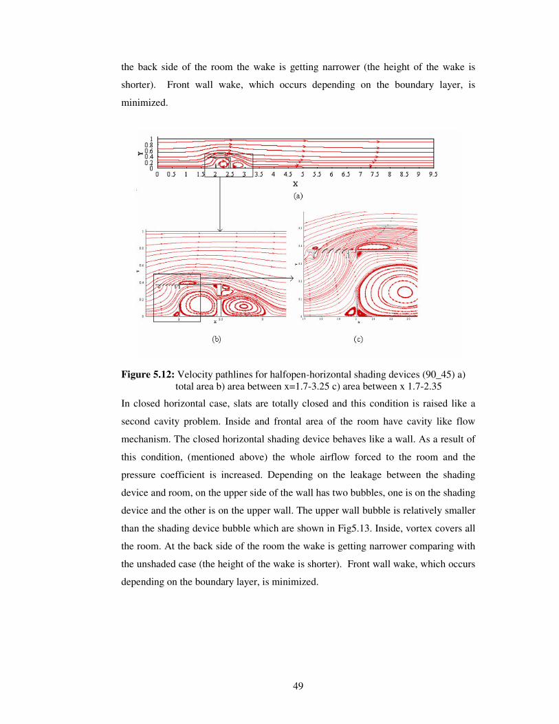
49

the back side of the room the wake is getting narrower (the height of the wake is

shorter). Front wall wake, which occurs depending on the boundary layer, is

minimized.

Figure 5.12: Velocity pathlines for halfopen-horizontal shading devices (90_45) a) total area b) area between x=1.7-3.25 c) area between x 1.7-2.35

In closed horizontal case, slats are totally closed and this condition is raised like a

second cavity problem. Inside and frontal area of the room have cavity like flow

mechanism. The closed horizontal shading device behaves like a wall. As a result of

this condition, (mentioned above) the whole airflow forced to the room and the

pressure coefficient is increased. Depending on the leakage between the shading

device and room, on the upper side of the wall has two bubbles, one is on the shading

device and the other is on the upper wall. The upper wall bubble is relatively smaller

than the shading device bubble which are shown in Fig5.13. Inside, vortex covers all

the room. At the back side of the room the wake is getting narrower comparing with

the unshaded case (the height of the wake is shorter). Front wall wake, which occurs

depending on the boundary layer, is minimized.

50

Figure 5.13: Velocity pathlines for closed-horizontal shading devices (90_0) a) total area b) area between x=1.7-3.25 c) area between x 1.7-2.35

Figure 5.14 is a short review of horizontal cases. It is easy to compare open, half-

closed and closed cases. The shapes of bubbles around and inside the room are seen

obviously. Especially the closed case has significant difference. The flow inside and

front of the room behaves like a cavity flow and the vortex on the upper wall has two

wakes. The smoothest airflow behavior around and inside the room occurs in the half

closed case due to the slat angle’s airflow forcement.

Figure 5.14: Pathlines comparison between slats of a) 90_0, b) 90_45, c) 90_90

51

5.2.3 Vertical Shading Devices

Vertical shading devices has three cases; open, half open, and closed as explained in

model definition part.

5.2.3.1 Velocity Profiles for Vertical Shading Devices

The velocity magnitude increases depending on the slat angles. When the case is

closed which means the angle of slat angle is 0, the maximum velocity is 5.5m/s. In

open-vertical case (slat angle is 90), velocity magnitude reaches 4.2m/s. Maximum

velocity for the half-closed vertical case (slat angle 45) is 6.5 m/s. The velocity

profiles of this cases summarized in Figure 5.15.

Figure 5.15: Velocity profiles for vertical shading devices and unshaded case at x=4.5h

5.2.3.2 Pressure Coefficient for Vertical Shading Devices

Pressure coefficients of the windward for vertical cases are drawn in Fig. 5.16. On

windward, pressure coefficient for closed case reaches at a value +5.8 where is

closed to the down of the windward. The minimum pressure coefficient is app. -3

where is closed to the upper wall intersection. On windward, pressure coefficient for

half_closed case reaches at a value +7 where is closed to the down of the windward.

The minimum pressure coefficient is app. –1.5 where is closed to the upper wall

52

intersection. Pressure coefficient for open case reaches at a value +3 where is closed

to the down of the windward. The minimum pressure coefficient is app. -3 where is

closed to the upper wall intersection.

Figure 5.16: Pressure Coefficient profiles for horizontal shading devices (0_90, 0_45, 0_0) and unshaded case on windward

On the upperwall that is shown in Fig.5.17, pressure coefficient for closed case

reaches maximum +0.7and min.-2.4. On the upperwall, pressure coefficient for

half_closed case reaches at a value +1.5where is closed to the down of the windward.

The minimum pressure coefficient is app. –0.25 where is closed to the upper wall

intersection. The pressure coefficient for open case max value is –0.5 and min is –

2.25. The shape of the pressure coefficient diagram on upper wall shows the pressure

distribution and gives an idea about the shape of the bubbles on the outside exterior

of the upper wall.

53

Figure 5.17: Pressure Coefficient profiles for horizontal shading devices (0_90, 0_45, 0_0) and unshaded case on upper wall

On leeward that is shown in Fig.5.18, pressure coefficient for closed case reaches

maximum –0.2 and min.-3.5. On the upperwall, pressure coefficient for half-closed

case reaches at a value +1.8 where is closed to the down of the windward. The

minimum pressure coefficient is app. –0.1 where is closed to the upper wall

intersection. The pressure coefficient for open case max value is –0.2 and min is –

0.8.

Figure 5.18: Pressure Coefficient profiles for horizontal shading devices (0_90, 0_45, 0_0) and unshaded case on leeward

54

5.2.3.3 Path lines for Vertical Shading Devices

The pathlines for vertical cases are analyzed in this part and drawn in Figures 5.18-

5.21. Each figure shows separate vertical cases, which are open, half-closed, and

closed cases, airflow on the solution domain and around and inside the room.

In open vertical case, slats directed the airflow to room. When looking at the

solution as general in Figure 5.19 there is three main vortexes on solution domain

where upper, inner and back sides of the room. Comparing the unshaded case and the

open vertical case, the shape of these vortexes are not changed unlike horizontal

cases The open slats directed the flow smoothly to the room and the airflow behaves

like unshaded case inside the room. The vortex is narrower and the bubble in front of

the front of the front wall, which occurs depending on the shear forces on the floor, is

bigger than the horizontal cases.

Figure 5.19: Pathlines for open-vertical shading devices (0_90) and unshaded case a) total area b) x=1.7-3.25 c) x= 1.8-2.35

In half closed vertical case, slats directed the airflow to the upper side of the room.

When looking at the solution domain as general in Fig 5.20, there is two main

vortexes on solution area where inner and back sides of the room. Due to the

movement of the airflow, the vortex inside the room covers almost all the room. The

bubble ,which normally seems on the upside of the upper wall, is getting minimum

comparing with the vertical cases. The wind ward and leeward’s vortexes are also

minimized.

55

Figure 5.20: Pathlines for halfopen-vertical shading devices (0_45) and unshaded case a) total area b) x=1.7-3.25 c) x= 1.8-2.35

Figure 5.21 shows the closed vertical case solution domain as general and detailed.

When looking at the general view, there seems three bubbles, where are inside and

backside of the room. The maiin difference from the other two vertical cases is the

location of the bubbles. Two of the three vertical cases occurs inside of the room

which are main vortex behavior and relatively small vortexes. The shape of the room

inside vortexes are caused by the leakage between the shading device and the room.

The shear layer vortex in front of the room is almost disappeared.

Figure 5.21: Pathlines for closed vertical shading devices (0_0) and unshaded case a) total area b) x=1.7-3.25 c) x= 1.8-2.35

56

Figure 5.22 is a short review of three vetical cases which gives an idea of the effects

of slats angle on vertical shading devices’ airflow. The shapes of the bubbles around

and inside the room are seen obviously. At the room inside flow behavior point, the

best case seems open vertical case. However, this condition causes a maximizing on

the windward and upperwall vortexes’.

Figure 5.22: Pathline comparison between three vertical cases a) 0_90 b) 0_45 c) 0_0

5.2.4 Diagonal Shading Devices

Diagonal shading devices has three cases; open, half open and closed as explained in

model definition part.

5.2.4.1 Velocity Profiles for Diagonal Shading Devices

The velocity magnitude increases depending on the slat angles. When the case is

closed which means the angle of slat angle is 0, the maximum velocity is 5.2m/s. In

open-diagonal case (slat angle is 90), velocity magnitude reaches 6.5 m/s. Maximum

velocity for the half-closed diagonal case (slat angle 45) is 4.6 m/s. The velocity

profiles of this cases summarized in Figure 5.23.

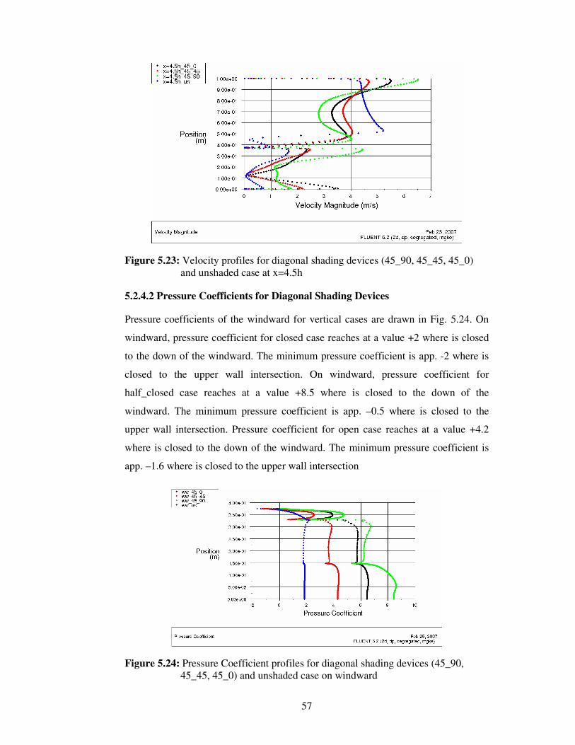
57

Figure 5.23: Velocity profiles for diagonal shading devices (45_90, 45_45, 45_0) and unshaded case at x=4.5h

5.2.4.2 Pressure Coefficients for Diagonal Shading Devices

Pressure coefficients of the windward for vertical cases are drawn in Fig. 5.24. On

windward, pressure coefficient for closed case reaches at a value +2 where is closed

to the down of the windward. The minimum pressure coefficient is app. -2 where is

closed to the upper wall intersection. On windward, pressure coefficient for

half_closed case reaches at a value +8.5 where is closed to the down of the

windward. The minimum pressure coefficient is app. –0.5 where is closed to the

upper wall intersection. Pressure coefficient for open case reaches at a value +4.2

where is closed to the down of the windward. The minimum pressure coefficient is

app. –1.6 where is closed to the upper wall intersection

Figure 5.24: Pressure Coefficient profiles for diagonal shading devices (45_90, 45_45, 45_0) and unshaded case on windward

58

On the upperwall that is shown in Fig.5.25, pressure coefficient for closed case

reaches maximum –2.2 and min.-2.6. On the upperwall, pressure coefficient for

half_closed case reaches at a value +0.5where is closed to the down of the windward.

The minimum pressure coefficient is app. –1.2 where is closed to the upper wall

intersection. The pressure coefficient for open case max value is 1.4 and min is –1.3.

The shape of the pressure coefficient diagram on upper wall shows the pressure

distribution and gives an idea about the shape of the bubbles on the outside exterior

of the upper wall.

Figure 5.25: Pressure Coefficient profiles for diagonal shading devices (45_90, 45_45, 45_0) and unshaded case on upper wall

On leeward that is shown in Fig.5.26, pressure coefficient for closed case reaches

maximum –1.25 and min.-2.25. On the upperwall, pressure coefficient for half-

closed case reaches at a value +0.5 where is closed to the down of the windward. The

minimum pressure coefficient is app. –0.75 where is closed to the upper wall

intersection. The pressure coefficient for open case max value is 1.7 and min is –

0.55.

59

Figure 5.26: Pressure Coefficient profiles for diagonal shading devices (45_90, 45_45, 45_0) and unshaded case on upper wall

5.2.4.3 Pathlines for Diagonal Shading Devices

The pathlines for diagonal cases are analyzed in this part and drawn in Figures 5.27-;

5.30. Each figure shows separate diagonal cases airflow on the solution area and

around and inside the room.

In open diagonal case, slats directed the airflow to both the upper side of the solution

domain and the inner side of the room whih is shown in Figure 5.27 in general and

detailed. In general view, there seems only two main vortexes ehere are inside the

room and leeward. In detailed figure, there seems also a vortex on the upper wall.

The main deifference for diagonal cases are the vortexes between the slats. These

vortexes prevent the airflow to the inside like a closed case but let the daylighting to

the inside.

60

Figure 5.27: Pathlines for open diagonal shading devices (45_90) and unshadedcase a) total area b) x=1.7-3.25 c) x= 1.8-2.35

In half closed diagonal case behaves like open diagonal case. There are differnces in

minumum scale like the shape of height of the room inside bubble and and the

location of the bubbles between the slats. There also an airflow between the slats and

it helps the daylighting.

Figure 5.28: Pathlines for halfopen diagonal shading devices (45_90) and unshaded case a) total area b) x=1.7-3.25 c) x= 1.8-2.35

As it is seen in Figure 5.29, the closed diagonal shading devices has two main

vortexes where are inside the room and leeward wall. The deatiled figures showas

that there also occurs a vortex on the upper wall. The shear layer vortex is

61

minimized.The closed slats direcst the flow in to the room smoothly. There is no

extra bubbles around the slats. As a result of this, the upper wall vortex is the

smallest in diagonal shadin devices.

Figure 5.29: Pathlines for closed shading devices (45_0) and unshaded case a) total area b) x=1.7-3.25 c) x= 1.8-2.35

Figure 5.30 summarizes the diagonal shading devices’ airflow movement. As a

summary, open and half open cases has vortexes between the slats. As a result of

these, the two cases behaves like closed case but in daylighting point it differs and is

relatively an advantage. The slat vortexes cause an enlargement on the upper wall

vortexes.

Figure 5.30: Pathline comparison between three diagonal cases a) 45_90 b) 45_45 c) 45_0

62

5.3 Summary

In this study, ten different case studies are discussed which are, one unshaded, three

horizontal shading devices, three vertical shading devices, and diagonal shading

devices. Velocity profiles in the centre of the room, pressure coefficients on the

windward, upper wall, and leeward, and finally pathlines of each case are shown in

figures.

Table 5.3 is summarized the velocities at x=4.5h and y=0.3h to discuss the

ventilation side. This point is taken to show results depending on the assumption that

a working person height will be at this point when he/she is working on a table. At

comfort levels, normally the velocity inside the room should be lower than 0.5 m/s.

Only unshaded, vertical closed and diagonal half closed cases are satisfied this

condition. Especially, horizontal closed case has a high velocity at this point which is

1.75m/s (6.3km/h) since the shading devices behaves as an upper wall and directed

all the airflow through the room, there is no leakage.

Vertical closed case seems the best situation at the point of view ventilation, velocity

at the workers level is 0.3 m/s. When we consider the day lighting issue, there is no

lighting gain through the window to the room because of the closed slats.

Table 5.3: Velocities for all cases at x=4.5h and y=0.3h

Case Velocity at x=4.5h, y=0.3h (m/s) Unshaded 0.3

Horizontal_closed (90_0) 1.75

Horizontal_halfclosed (90_45) 0.5

Horizontal_open (90_90) 0.9

Vertical_closed (0_0) 0.3

Vertical_halfclosed (0_45) 0.9

Vertical_open (0_90) 0.5

Diagonal_closed (45_0) 0.7

Diagonal_halfclosed (45_45) 0.4

Diagonal_open (45_90) 1.3

The best decision about the selection of the shading devices can be decided

considering the heat management and the 3D CFD solutions. Because of the

buoyancy effects, the natural ventilation speed would affect in real life, there also

63

occurs extra forces and loses depending on the third dimension. This study can be

used as a baseline for 3D simulations and energy coupled solutions.

Table5.4: Maximum and minimum pressure coefficients for all cases

Cd windward Cd upperwall Cd leeward Case

Max Min Max Min Max Min

Unshaded +2.3 -1.5 -2.27 -2.6 -1.3 -2.2

Horizontal_closed (90_0) 27 9.5 12 9 11 7.5

Horizontal_halfclosed (90_45) 5 -2 0.5 -1 1 -1

Horizontal_open (90_90) 4 -3 1.95 -1.5 -1.2 -2.2

Vertical_closed (0_0) 5.8 -3 0.7 -2.4 -0.2 -3.5

Vertical_halfclosed (0_45) 7 -1.3 1.5 -0.25 1.8 -0.1

Vertical_open (0_90) 3 -3 0.5 -2.25 -0.2 -0.8

Diagonal_closed (45_0) 2 -2 -2.2 -2.6 -1.25 -2.25

Diagonal_halfclosed (45_45) 8.5 -0.5 0.5 -1.2 0.5 -0.75

Diagonal_open (45_90) 4.2 -1.6 1.4 -1.3 1.7 -0.55

Table 5.4 is a short review of the pressure coefficients for all cases. It is practical

way to compare all studies Cps on windward, upper wall and leeward. Maximum

pressure coefficient occurs on horizontal closed case for all three walls because of

the shading device. Horizontal closed shading device behaves like wall and forced

directed the airflow to the room. This action raised extra forces on the room walls’

and this causes an increase on the pressure coefficient. This case also seems a

problem at the view of daylighting. It has a positive gain in daylighting when we

compare it with the case vertical closed. The best results and comments can be done

after applying a simulation on daylighting

.

64

6. CONCLUSION

In the present work the effects of wind differences on the natural ventilation is

introduced. Exterior shading devices used as a tool for controlling the wind effects

inside the buildings. The slat angles and positions of the shading devices affect the

airflow mechanisms and the natural ventilation of the buildings.

Energy issue has become a key concern because of the environmental and economic

reasons among the countries all around the world. Countries are searching ways to

reduce the energy consumption in order to ensure global energy sustainability.

Buildings are significant energy consumers and have an important role on the energy

context so that they have a priority in the many countries policies.

Saving energy is the most cost effective way to meet our future energy needs and to

prevent the air pollution for the indoor and outdoor environment. Buildings have a

high potential for energy savings. Many Governments around the world are

enhancing their building energy codes aiming to limit the energy consumption at a

minimum level possible. In order to ensure the energy limitations, the energy

consumption level of a building should be tried to keep at a minimum.

As an effective way to succeed energy consumption is natural ventilation. The cross

ventilation inside the buildings lowers the energy needing for cooling. The shading

devices especially used in tropical climates. The position of the shading devices and

various slat angles affect the natural ventilation.

The pressure disturbances caused by wind and buoyancy is an effective way to

optimize the natural ventilation. Using shading devices the wind effect could be

controlled on the building facade.

Computational or wind tunnel model could be used for utilizing the best shading

device position and slat angle. Wind tunnels are limited with the flexibility of the

65

model, labor costs and model costs. In CFD method, it has a wide range of model

description to choose the best way. Comparing with the wind tunnel model, it has

only computational costs. In this research, GAMBIT / FLUENT which is a

commercial CFD package is used for analyzing the air change phenomena of inside

and around the building and the shading devices.

The results of the case studies, horizontal (open, half_closed, closed), vertical (open,

half_closed, closed), and diagonal (open, half_closed, closed) shows that the vertical

shading devices lowered the airflow of building inside.

For the future work, the boundary conditions for the computational solution could be

modified for the real conditions (wind velocity, natural conditions etc.). An

algorithm could be written to define the wind velocity and ABL. The radiation

models and energy equations could be solved and the solar gains for model could be

calculated.

Furthermore, the model could be defined and solved in 3-D and not only horizontal

slats solved but also vertical slats can be analyzed. A compact relation between wind

tunnel experiments and computational model can be sustained.

In addition to this, daylighting effects of shading devices could be considered and

included into the solution area.

66

7. REFERENCES

Allard F., 1998, Natural Ventilation in Buildings: A Design Handbook, James& James Ltd, London.

Blazek, J., 2001, Computational Fluid Dynamics: Principles and Applications, Elsevier, London.

Bottema, M., 1980, Wind climate and urban geometry, Ph.D. Thesis, Eindhoven University of Technology, Eindhoven, The Netherlands.

BSI, 1991, Code of Practice for ventilation principles and designing for natural ventilation, British Standard, BS5925.

Chen, Q., 1995, Comparison of different k-e models for indoor air flow computations, Numerical Heat Transfer, Part B- Fundamentals 28(3): 353-369.

Chen, Q., 2004, Using computational tools to factor wind into architectural environment design, Energy and Buildings(in press).

Chen, Q. and Xu, W., 1998, A zero-equation turbulence model for indoor airflow simulation, Energy and Buildings 28:137-144.

CIBSE AM10, 1997, Natural ventilation in non-domestic buildings, Chartered Institute of Building Services Engineers, Application Manual.

CIBSEAM Briefing8, 2003, Reducing emissions through energy efficiency-key issues to edress in designing and operating buildings.The Chartered Institution of Building Services Engineering. London.

Cook, M. J., Ji, Y., and Hunt, G.R., 2003, CFD modelling of natural ventilation: combined wind and buoyancy forces, International Journal of Ventilation1 (3): 169-179.

Cook, N.J., 1985, The designer’s guide to wind loading of building structures-Part1: Background, damage survey, wind data and structural classification. Butterworths, London, UK.

Desam, P.R., 2003, Cfd_Fluent Lecture Notes, University of Utah.

Etheridge, D.W., 2000, Unsteady flow effects due to fluctuating wind pressures in natural ventilation design-mean flow rates, Building and Environment 35(2):11-133.

Fluent , 2006, Fluent version 6.2 user’s manual. URL: www.fluent.com/software/fluent /index.htm

Gan, G., 1999, Lectures Notes-Building Ventilation, Msc course in Renewable Energy and Architecture, University Nottingham.

Heiselberg, P., 1999, The hybrid ventilation process- theoretical and experimental work, Air Infiltration Review 21(1).

67

Hunt, G.R. and Linden, P.F., 1999, The fluid mechanics of natural ventilation-displacement ventilation by buyocancy-driven flows assisted by wind, Building and Environment 34(6):707-720.

Jiang, Y.D., Alexander, H., Jenkins, Arthur, R., and Chen, Q., 2003, Natural ventilation in buildings: measurement in a wind tunnel and numerical simulation with large-eddy simulation, Journal of Wind Engineering and Industrial Aerodynamics 91(3): 331-353.

Launder, B.E., Spalding D.B., 1974, The numerical computation of turbulent flows, Computer Methods in Applied Mechanics and Engineering 3: 269-289.

Lechner N., 2000, Heating, Cooling, Lighting: Design Methods for Architects, 2nd ed., John Wiley & Sons, Inc.

Liddament, M. W., 1991, A review of building air flow simulation, AIVC Technical Note 33, Air Infiltration and Ventilation Centre, Coventry, UK.

URL: www.aivc.org/Publications/Technical_reports/TN33.html

Li,Y., Delsante, A., Symons, J.G., Chen, L., 1998, Comparison of zonal and CFD modelling of natural ventilation Centre in a thermally stratified building., 6th International Conference on Air Distribution in Rooms-Roomvent 98, Stockholm, Sweden.

Nishizawa, S.T., Sawachi, T., Narita, K., Seto, H. And Ishikawa,Y., 2003, A wind tunnel sull scale building model comparison between experimental and CFD results based on the standard k-e turbulence representation. International Journal of Ventilation 2(4): 419-429.

Ok,V., Turkmenoglu, N., 2005, Investigation of the effects of the solar control elements on interior air movements, Unpublished doctoral dissertation, ITU, İstanbul.

Straw, M.P., 2000, Computation and measurements of wind induced ventilation, PhD thesis. University of Nottingham, UK.

URL: www.nottingham.ac.uk/~evzngw/download.html

Tennekes, H. and Lumley, J., 1972,A First Course in Turbulence. The MIT Press, Cambridge, Massachusetts.

Tomoyuki, E., Kurabuchi ,T., Ishii, M., Komamura, K., Maruta, E., and Sawachi,T., Study on the Numerical Predictive Accuracy of Wind Pressure Distribution and Air Flow Characteristics, International Journal of Ventilation, Volume4.

Versteeg, H.K., Malalasekara, W., 1995, Introduction to computational fluid dynamics, the finite volume method. Longman Scientific & Technical, Harlow.

URL: www.wind.ttu.edu

68

APPENDIX A

The solver definitions of Unshaded case FLUENT Version: 2d, dp, segregated, rngke (2d, double precision, segregated, RNG k-epsilon) Release: 6.2.16 Title: Unshaded - fine mesh Models Model Settings -------------------------------------------------------------------------------------------- Space 2D Time Steady Viscous RNG k-epsilon turbulence model Wall Treatment Enhanced Wall Treatment Functions RNG Differential Viscosity Model Disabled RNG Swirl Dominated Flow Option Disabled Heat Transfer Disabled Solidification and Melting Disabled Species Transport Disabled Coupled Dispersed Phase Disabled Pollutants Disabled Soot Disabled Solver Controls --------------- Equations Equation Solved ------------------------------- Flow yes Turbulence yes Numerics Numeric Enabled -------------------------------------------------------------- Absolute Velocity Formulation yes Relaxation Variable Relaxation Factor ----------------------------------------------------------------- Pressure 0.2 Density 1 Body Forces 1 Momentum 0.4 Turbulence Kinetic Energy 0.4 Turbulence Dissipation Rate 0.4 Turbulent Viscosity 0.5 Linear Solver

69

Solver Termination Residual Reduction Variable Type Criterion Tolerance ------------------------------------------------------------------------------------------ Pressure V-Cycle 0.1 X-Momentum Flexible 0.1 0.7 Y-Momentum Flexible 0.1 0.7 Turbulence Kinetic Energy Flexible 0.1 0.7 Turbulence Dissipation Rate Flexible 0.1 0.7 Discretization Scheme Variable Scheme ------------------------------------------------------------- Pressure Second Order Momentum Second Order Upwind Turbulence Kinetic Energy Second Order Upwind Turbulence Dissipation Rate Second Order Upwind Solution Limits Quantity Limit ---------------------------------------------------------- Minimum Absolute Pressure 1 Maximum Absolute Pressure 5e+10 Minimum Temperature 1 Maximum Temperature 5000 Minimum Turb. Kinetic Energy 1e-14 Minimum Turb. Dissipation Rate 1e-20 Maximum Turb. Viscosity Ratio 100000

70

RESUME

She was born in Kocaeli in 1980. She finished Oruc Reis Anatolian High School in

Kocaeli. She graduated from Istanbul Technical University as Mechanical Engineer

in 2003. She started her master’s degree in Mechanical Engineering department

Thermo-Fluid Program in ITU. She studied in Stuttgart University of Applied

Sciences (SAS) in 2004 in the framework of Erasmus Exchange Program. She

worked in SAS as research assistant between March 2006 and January 2007.