ISSN 11 75-1 584

MINISTRY OF FISHERIES

Te Tautiaki i nga tini a Tangaroa

Calculation and interpretation of catch-per-unit-effort (CPUE) indices

A. Durn S. J. Harley

I. J. Doonan

B. Bull

New Zealand Fisheries Assessment Report 2000/1 February 2000

Calculation and interpretation of catch-per-unit-effort (CPUE) indices

A. Dunn S. J. Harley I. J. Doonan

B. Bull

NIWA PO Box 14 901

Wellington

New Zealand Fisheries Assessment Report 200011 February 2000

Published by Ministry of Fisheries Wellington

2000

0 Ministry of Fisheries

2000

Citation: Dunn, A., Harley, S.J., Doonan, I.J., & Bull, B. 2000: Calculation and interpretation of catch-per-unit effort (CPUE) indices.

Nau Zealand Fisheries Assessment Report 2000/1.44 p.

This series continues the informal New Zealand Fisheries Assessment Research Document series

which ceased at the end of 1999.

EXE.CUTIVE SUMMARY

Dunn, Amy Harley, SJ., Doonan, IJ. & Bull, B. 2000: Calculation and interpretation of catch-per-unit-effort (CPUE) indices. N.Z. Fisheries Assessment Report 2000/1.44 p.

This report is in fulfilment of the requirements for Objective 4 of Project SAM 9801, Improved Methods for Fish Stock Assessment Modelling. The objective was 'To determine when catch and effort data should be used to construct biomass indices." This report reviews the literature, investigates the empirical relationship between a sample of observed CPUE and associated, but independent, biomass indices, and discusses guidelines for calculating and interpreting CPUE data.

The assumption of a proportional relationship between CPUE and abundance has often been criticised, and m a . authors warn that the assumption of proportionality can be very misleading when estimating abundance. However, there is still a persistent belief that changes in CPUE index changes in abundance, though the precise nature of the relationship between CPUE and abundance may be uncertain. The literature is characterised by conclusions derived from theoretical fisheries which show that, in general, CPUE is not proportional to biomass, but few studies report on any empirical relationships between CPUE and abundance.

We present an analysis of empirical CPUE data for a range of New Zealand and international (non-New Zealand) fisheries. We compared CPUE with independent biomass observations and with estimated biomass resulting from stock reduction models, estimating a 'shape' parameter indexed by B. The analysis suggested that although the relationship may range from hyperstable to hyperdepletion (i.e., B < 1 or B > l), a proportional relationship may be an adequate approximation for some stocks (although inference and generalisation based on these data should be treated with extreme caution). The range of confidence bounds for the estimates of B suggest that values between 0.5 and 2 may encompass most relationships that might be found for a wide range of stocks or species. Hence, a possible interpretation of these results is that the assumption of proportionality may not be inadequate, although, clearly, more research on possible values of B is required. In particular, the impact of a hyperstable (B = 0.5) or hyperdepletion (B = 2) relationship on stock assessments needs to be investigated.

Ministry of Fisheries Fishery Assessment Working Groups (WGs) use a number of unwritten rules-of-thumb to assist in determining if calculated indices provide useful information of abundance or change in abundance for individual fish stocks. Such guidelines are often not based on theoretical or even empirical rules and differ widely between WGs in both f o m and implementation, and there appears to be little consistency between different WGs, stocks, or analyses. We explored these decisions for aspects of good practice and combined these with general advice for model fitting given in the statistical literature. We develop four components for inclusion in the analysis of CPUE, and recommend that CPUE analyses include discussion of these where practical. The components are (1) definition of the relationship between CPUE and abundance, (2) assessment of data adequacy, (3) methods of model fitting and model validation, and (4) evaluation of the CPUE index.

It is clear that there are no simple recipes for calculating CPUE indices, even when appropriate steps have been taken in the analysis of catchleffort data. Simply put, there are no easy answers, and .every analysis requires a good understanding of both the fishery and the factors that can influence the CPWabundance relationship.

1. INTRODUCTION

Catch and effort data are often used to construct biomass indices for fish stocks on the assumption that catch-per-uniteffort (CPUE) is proportional to abundance. Whether it is calculated as a simple ratio of catch to effort or via a more complex standardisation process (Gavaris 1980), the basis on which CPUE is assumed to index abundance is the observation that the mean catch from a fish stock tends to decrease when there is a decrease in either population density or the amount of effort expended (Bishir & Lancia 1996). This leads to the functional equation, T& = qN, where T is the expected catch, E is effort, and N is abundance. The parameter q is considered a measure of 'catchability' and is usually called the catchability coefficient.

The terms catch, effort, abundance, and catchability are used widely within the literature, often in different contexts. The differences in definitions of terminology can lead to some confusion when reviewing this topic. For this paper, we use a fishing episode to indicate the fishing activity leading to the catch and requiring associated effort - which need not be the result of a single discrete action. For example, using the catch from a day's fishing or the catch obtained from a series of set nets, gives a measure of CPUE in terms of catch-perday or catch-per-set respectively. For larger trawl and longline fisheries, CPUE has usually been determined as, for example, the catch-per-kilometre-towed or catch-per-hook The implication is that an episode of fishing can range fkom a single cast of a net, an aggregated count of fishing activity, or even the result of a period of fishing time.

Abundance is the total biomass or total number of fish for some fish stock, over a specified period of time and space, and can be considered the biomass or number of fish in the population from which the 'sample' of catch was drawn. This is an important constraint, as CPUE will reflect relative abundance only over the temporal and spatial domain encompassed by the data.

The relationship between relative abundance and catchieffort is defined by the catchability coefficient q and represents, in part, the relationship between the localised fish density and the 'efficiency' of fishing gear (Arreguin-Shchez 1996). When catchability is constant, there is a proportional relationship between CPUE and abundance. Other, more complex forms can be derived by assuming a functional form for q.

For CPUE measures to be useful, catchleffort should be defined so that it is a measure of the relative density of the fish stock, and hence of relative abundance. Although definitions of catch and effort are straightforward, the resulting CPUE is often a composite mixture of many aspects of a fishing process. The different measures of catch and effort employed for the different fish stocks lead to very different measures of CPUE. For example, New Zealand CPUE analyses typically use measures of effort such as fishing day, distance towed, and hooks set, giving CPUE measures of kg-perday, kg-per-kilometre-towed, and fish-per-hook. Measures of effort have also been extended to include aspects of fishers' searching time (representing time lost to fishing due to the time taken to locate a suitable fishing location) and handling time (representing the time lost to fishing due to the time taken to process the previous catch). Such extensions not only account for the amount of time fishing gear may be in the water for example, but also for combinations of fishing, searching, and handling time (Hilbom & Walters 1987, 1992). This not only attempts to incorporate a measure of fish density over the less productive parts of the fishing ground, but also to capture other explanatory (or confounding) elements of the fishing process. Examples of this effort measure are daily aggregated data, often present in New Zealand CPUE analyses using CELR data. Examples in the published literature include whale catch-per-search-time-hour (Cooke

1985>, purse seine CPUE based on catch-per-hour (Gaertner et al. 1998), and catch-per-net- per-week for shovelnose guitarfish (Salazar Hermoso & Villavicencio Garayzar 1999).

For this paper, we consider that the aim of CPUE analysis is to determine a set of relative abundance indices over a spatial and temporal domain for a specific fish stock The relationship between the CPUE indices and true abundance is assumed to be proportional when used to fit or tune stock assessment models. Unfortunately, ignorance of the level of true abundance does not often allow this assumption to be either tested or validated. If the true abundance were known, CPUE indices would not be required.

The assumption of a proportional relationship between CPUE and abundance has long been criticised in the scientific literature, and a wide range of reasons for non-proportionality have been cited. Many authors warn that the assumption of proportionality can be very misleading when estimating abundance (e.g., Hilborn & Walters 1992), although few present evidence for their claim. However, there is still a persistent belief that changes in CPUE index changes in abundance, though the precise nature of the relationship between CPUE and abundance may be uncertain.

There appears to be little useful empirical work on relationships between CPUE indices and abundance in the published literature. This is due, in part, to the difficulties of obtaining accurate abundance measures for individual fish stocks over a suitably long period for comparison with CPUE indices. In addition, the imprecise nature of fisheries research implies that relationships, where found, may support a wide range of plausible (or even implausible) hypotheses.

This report reviews the published literature on the relationship between CPUE and abundance, and considers how we may use and interpret the resulting CPUE indices as a part of the stock assessment and management process. We investigate the assumption of proportionality between CPUE and abundance and consider an alternative model. Even if we can assume a monotonic relationship between CPUE and abundance for some fish stock, issues relating to data quality and data adequacy are likely to dominate decisions of the usefulness and acceptability of any calculated index. We present a simulation study that suggests information on the nature of the relationship between CPUE and abundance can not often be determined from the data. Ministry of Fisheries Fishery Assessment Working Groups (WGs) use a number of unwritten rules-of-thumb to assist in determining if calculated indices provide useful information of abundance or change in abundance for individual fish stocks. Such guidelines are often not based on theoretical or even empirical rules and differ widely between WGs in both form and implementation. We explore these decisions for aspects of good practice and combine these with general advice for model fitting given in the statistical literature. We also present an analysis of empirical CPUE data for a range of New Zealand fisheries, comparing CPUE with more direct, independent biomass observations, and estimated biomass resulting from stock reduction models. We use these results to develop methods for assessing data adequacy and for investigating CPUEIabundance relationships. Finally, we present a list of guidelines for the calculation and interpretation of CPUE indices.

2. A REVIEW OF THE RELATIONSHIP BETWEEN CPUE AND ABUNDANCE

When CPUE is used to estimate the biomass of a stock, a relationship between CPUE and abundance is assumed. Usually this relationship is assumed to be proportional. Hilbom & Walters (1992) provided an introductory review of CPUE, beginning with the question "... what type of relationship should we expect to see between CPUE and abundance?'As a

partial answer, they suggested three general relationships; hyperstability (where CPUE stays high with decreasing abundance), proportionality (where CPUE is proportional to abundance), and hyperdepletion (where CPUE decreases much faster than abundance), (see Figure 1). This is a useful starting point from which to discuss the relationship between CPUE and abundance, but we found few empirical studies within the published literature on the types of relationships found in practice.

The assumption of a proportional relationship between CPUE and abundance is the simplest relationship that can be assumed, and is the assumption made by most of the New Zealand stock assessments that use CPUE. However, for a proportional relationship to be true, not only must fishing effort be random with respect to distribution of fish biomass, but the catchability must be constant over space and time (HiIbom & Wdters 1987, 1992, Dunn & Doonan 1997). A consequence of the fust condition is that fishers allocate effort independently (deLury 1947).

Abundance

Figure 1: The shape of the three general relationships between CPUE and abundance: hyperstabiity, proportional, and hyperdepletion (from Hilborn & Wdters, 1992).

Hilbom & Walters (1992) claimed that a proportional relationship ". . .has been demonstrated to be wrong in almost every case where it has been possible to test - simply stated it is almost impossible for this relationship to be true, and those who use it are running severe risks". However, they offered no evidence for their claim. Their conclusion is by no means novel. Criticism of CPUE-based approaches to estimating abundance have been present in the scientific literature for almost as long as the method itself. Seber (1982) attributed the first use of catchleffort methods to estimating bear populations in Norway in 1914, and one of the first applications of this method to fisheries data appears to be that of Baranov (1918). He employed catch data in developing a herring model, assuming that biomass was uniformly distributed and that fish were immobile. Even in such an early study, Baranov suggested that CPUE would not directly represent abundance if fishers concentrated effort on larger schools of fish. Paloheimo & Dickie (1963) reviewed the CPUE literature fiom the first half of the 20" century, and concluded that explicit consideration of the heterogeneity in fish distributions and directed allocation of fishing effort was required to model catchleffort data.

They went on to develop a set of equations that looked at simple fish schooling behaviour in a theoretical fishery, and found that CPUE depended not only on the overall abundance, but on the size of schools and their respective densities as well.

More recently, research has focused on the functional form of the catchability coefficient. A number of authors have observed that catchability appears to change with changes in abundance (McCall 1976, Ulltang 1976, Peterman & Steer 1981, Bannerot & Austin 1983, Angelsen & Olsen 1987, Quinn 1987, Csirke 1988, Crecco & Overholtz 1990, Gordoa & Hightower 1991, Rose & Leggett 1991, 1993), with most concluding that catchability appeared to increase at low levels of abundance. Hilborn & Walters (1992) suggested that effects of fishers' search time, fish handling time, and non-random search fishing strategies may account for some of the non-linear effects in the relationship between CPUE and abundance. Dunn & Doonan (1997) showed that the spatial redistribution of the fish stock can alter the relationship between CPUE and abundance (see also Gillis et al. 1993). Other theoretical work has been conducted on aspects of fisher strategy and spatial redistribution of fish stocks, but has not been linked explicitly back to CPUE. For example, Vignaux (1996) investigated fishing strategy in a New Zealand hoki fishery, suggesting that fishers use the location of the fishing fleet as a proxy of fish location to locate high density patches of fish, and Swain & Sinclair (1994) investigated how measures of the spatial distribution of fish stocks influence catchability.

The few papers that investigate relationships between CPUE and abundance find little evidence for a proportional relationship. Cooke (1985), in an investigation of the relationship between CPUE and whale abundance, questioned the use of CPUE in assessing whale stock status and concluded that there was little evidence for assuming a proportional relationship for the whale data. However, he did not discuss evidence for alternative relationships. Worthington et al. (1998) looked at CPUE measures for an abalone fishery, and suggested that the non-linear relationship between catch and effort would lead to a non-proportional relationship between CPUE and abundance. An exception to the failure to find a proportional relationship between CPUE and abundance within published literature is that of Richards & Schnute (1986). They compared CPUE from angling from a surface vessel to direct counts from a submersible in regions of different abundance, and found for the two single-species they investigated that "...the relationship appears to be one of strict proportionality". However, for this study, assumptions of constant catchability and random fishing with respect to the distribution of fish appear to be plausible, and are essentially part of the study design.

A complete understanding of how the fishery functions (not only in fisher behaviour, but also in changes in the spatial distribution of the fish stock caused by changes in abundance) is an essential component of any CPUE analysis. It is relatively easy to create hypothetical scenarios where CPUE increases with declining abundance or vice-versa. For example, consider a fish stock that has uniformly distributed background scatter combined with localised high density schools of fish when at levels of high abundance. Further assume that as abundance declines, the high density schools remain, but the background scatter reduces. If fishing at high abundance takes place over the background scatter, and moves towards the localised schools as abundance declines, then CPUE may appear to increase with declining abundance. This hypothetical scenario implies a change of fishing practice fiom one of random fishing to one of targeted fishing with decreases in abundance, implying that fishers do not seek to maximise catch rates, but rather seek to maintain catch above some baseline or threshold. Both Hilborn (1985) and Cooke (1985) emphasised the importance of fully understanding the fishing process in order to understand the relationship between CPUE and abundance.

Where the nature of the relationship can safely be assumed, CPUE can provide a useful index of relative stock abundance. However, there has been little work on the nature of such relationships, and even less on the specific relationships for individual stocks. The assumptions of random fishing with respect to fish distribution and constant catchability would seem unlikely for most New Zealand stocks. This leads us to suggest that a proportional relationship between CPUE and abundance should not be assumed without some scientific consideration. Moreover, this raises the question of whether any relationship exists at all, and, if so, what form does it take?

3. DETERMINING THE CPUEIABUNDANCE RELATIONSHIP

The comparison of CPUE indices with other, independent, measures of abundance or biomass may give some insight into the nature of the relationship between CPUE and abundance. We introduce a two parameter model (with shape parameter B and scale parameter a) that describes a simple family of monotonic relationships, and use this model to investigate the relationship between CPUE and other measures of abundance.

By comparing CPUE to relative abundance indices resulting from (a) trawl and acoustic surveys, and (b) estimates of relative biomass determined fi-om stock assessment models, we find empirical values of B for a range of New Zealand and non-New Zealand fish stocks. However, there are few data sets where both CPUE indices of abundance and alternative, independent estimates of biomass exist. Where such data exist, there are often only a few data points from both series that cover the same period in time, so the abiity to infer plausible values of B or examine patterns specific to families of stocks, species or fishing methods, is limited.

Model structure

We assume a monotonic relationship between CPUE (C) and non-CPUE abundance (N) .indices, which has the functional form

The scale parameter a is a nuisance parameter and is ignored for this analysis. Hence we can describe the relationship between C and N by the shape parameter B.

Figure 2 shows the shape of the relationship between CPUE and abundance for values of the shape parameter B. We can interpret the shape when B -c 1 as that of a hyperstable fishery (as described by Hilborn & Walters 1992). B > 1 corresponds to hyperdepletion and B = 1 corresponds to proportionality.

As we observe abundance with observational error (i.e., both CPUE and the alternative abundance indices are estimates of true abundance), we assume that we observe C and N with random error. We derive a structural relationship between C and N by taking logs of Equation [I] and assuming that we observe n paired samples of log (c) with error 6 , and log(^) with error < .

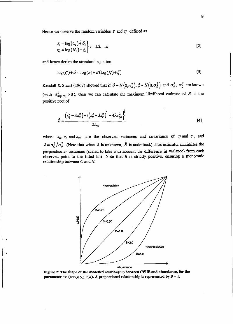
Hence we observe the random variables E and q , defined as

and hence derive the structural equation

Kendall & Smart (1967) showed that if 6 - N (o,~:), 5 - N (0,052) and 0: , 0; are known

(with o&,,) >O), then we can calculate the maximum likelihood estimate of B as the

positive root of

where $, s, and sqE are the observed variances and covariance of q and E , and

1 = $/oi . (Note that when 1 is unknown, d is undefined.) This estimator minimises the

perpendicular distances (scaled to take into account the difference in variance) from each observed point to the fitted line. Note that B is strictly positive, ensuring a monotonic relationship between C and N.

Abundance

Figure 2: The shape of the modelled relationship between CPUE and abundance, for the parameter B E (0.25,0.5, I, 2.4). A proportional relationship is represented by B = 1.

The confidence interval for i = tan (0) can be estimated (using maximum likelihood) as

where t is the appropriate Students-t deviate with (n-2) degrees of freedom for the confidence interval chosen.

Properties of the estimator i of the shape parameter B

We investigated the ability of i to estimate B using simulation. We assumed we observed n paired samples of CPUE (0 and non-CPUE (N) indices with functional relationship

C = d V B , and that C and N are independently and identically distributed (i.i.d.) observations with lognormal errors with constant C.V. Further, we assume that the n paired samples of C and N were observed with a percent reduction in the true underlying biomass described by the parameter r.

Simulated data were generated that contained 4, 8, 12, 16, and 20 pairs of observations (n). The values of n were chosen to contain the range of observed lengths of the series from New Zealand fish stocks detailed later in this report. Data series of such lengths are typical of biomass estimates available for stock assessment. Values of B were chosen to encompass the range of plausible shapes of relationship between CPUE and non-CPUE abundance indices (i.e., hyperstable, proportional, and hyperdepletion). Simulations were canied out assuming three levels of observation error, C.V. = 0.1,0.2, and 0.3. Estimates of B were calculated using

Equation [4], with observation error assumed known (i.e., we assume that we h o w 0: and

02 are equal, and hence set A =I). A total of 500 simulated sets of observations were

generated for each combination of the input parameters (summarised in Table I), and k was calculated for each. Median and 95% percentiles from the simulated distribution were determined. The simulation software was written using S-Plus (MathSoft 1997).

Table 1: The simulation input parameters

Shape No. of observed % reduction in Observation C.V. parameter (B) points (n) biomass (r)

showed that generally, in scenarios with very large reductions in the underlying iomass, reasonable estimates of the shape of relationship between indices were obtained.

Conversely, in scenarios with only a small change in the underlying biomass, little inference '7 >, was possible. The results are summarised in Figure 3, and Tables C1, C2, and C3 in

Appendix C tabulate the results for the simulations where the observed C.V. = 0.1,0.2, and 0.3 respectively.

With few observations (n = 4 or 8), a large reduction in the underlying biomass was necessary to accurately estimate the shape parameter. With strongly hyperstable relationships, the relative change in CPUE is small compared with the change in observed biomass and the data appeared to contain little information on the value of B, irrespective of the true B. With increased numbers of observations (n = 16 or 20), slightly better estimates of B were obtained and 95% percentiles were reduced only slightly. Reductions in c.v. from 0.3 to 0.1 improved the estimation performance slightly.

For B = 1, a reduction in biomass of at least 50% and in some cases 75% was required to distinguish between proportional, strongly hyperstable, or strongly hyperdepleted relationships. The increased number of observations from 4 to 20 had minor impact, only improving precision slightly. When the underlying biomass was reduced by a smaller proportion (i.e., r = 12.5% or 25%), the shape parameter was impossible to determine with any useful accuracy. In particular, tended to approximate 1 irrespective of the true value (i.e., was strongly biased).

The simulated data showed that scenarios with a strong hyperstable relationship were difficult to identify, even when the underlying biomass reduced considerably. With a weakly hyperstable relationship, some information on the shape parameter B can be inferred, though only to the extent of excluding strong hyperdepletion.

Clearly, increased numbers of observations would enable a more accurate estimate of B, as would much reduced levels of observation error, particularly when there were only small changes in the underlying biomass. Unfortunately, few New Zealand fish stocks have paired sets of observations greater than n = 10 (see Table 2), i d increased accuracy for biomass indices is impractical. Without more observations or greatly increased precision in abundance estimates, estimation of the nonlinearity of the relationship between CPUE and abundance will likely be very imprecise, except where stock biomass has declined to a small fraction of original values.

Comparison of New Zealand and non-New Zealand CPUE and non-CPUE data We compared CPUE and non-CPUE indices from New Zealand stock assessments published in Ministry of Fisheries Research Reports, N.Z. Fisheries Assessment Research Documents (FARDs), and NIWA Technical Reports. In addition, we calculated CPUE for stocks where source data was readily available but no up-to-date B U E index had been calculated. CPUE indices were, however, considered for stocks only where an alternative and independent biomass index was also available, and where both sets of indices index the same period in time, with at least two sets of paired observations. We consider non-CPUE indices resulting from trawl surveys and acoustic surveys (and labelled collectively as survey indices), and estimates of relative biomass indices resulting from stock assessment models that were fitted without using CPUE data (and labelled as model indices). (Table A1 in Appendix A details the indices available for each species and stock)

Selected data from overseas sources (non-New Zealand stocks) were also considered where there were source documents with both the CPUE and survey biomass index tabulated. Access to this data was limited to published abundance indices only, and no data were available from model outputs on estimated biomass for these stocks. The data are summarised in Table A2 in Appendix A.

0.0 0.25 0.50 0.75 1.00

% reduction in biomass

0.0 0.25 0.50 0.75 1.00

% reduction in biomass

0.25 0.50 0.75

% reduction in biomass

-. -

0.0 0.25 0.50 0.75 1.00 0.0 0.25 0.50 0.75 1.00

% reduction in biomass % reduction in biomass

Figure 3: Median i of the simulated distribution, for the shape parameter B for (a) B = 0.25 @) B = 0.5 (c) B = 1.0 (d) B = 2.0 (e) B = 4.0, against % reduction in biomass r e (12.5.25.0,50.0,75.0)

and number of observations n E (4,8,12,16,20), with CPUE and biomass observation error c.v = 0.2. True B for each plot is shown as a dashed horizontal line, with the number of observations plotted as text. 95% percentiles for n = 8 are shown as grey vertical lines.

Plots- of the empirical relationship between (a) CPUE indices and survey indices and (b) CPUE indices and model indices are shown in Figures B 1 and B2 for New Zealand stocks. Similarly, plots of CPUE indices and survey indices for the non-New Zealand stocks are shown in Figure B3. The indices are all standardised to have maximum 1; grey arrows drawn between points show the annual change from point to point. CPUE indices are shown as the y-axis, with the non-CPUE index shown as the x-axis. Stocks are shown as the plot title, and axis labels give the detail of each respective series. In addition, dotted lines represent a break in the series of at least 1 year.

No New Zealand fish stocks (37 in total) had a paired CPUE and survey index with more than 7 data points, and most were 4 or less. Fewer fish stocks had model indices of relative biomass (22), although these had longer (and hence more useful) paired sets of observations. Model indices were generated without the use of CPUE indices, and the degree to which these estimates reflect the true underlying biomass is unknown. The properties of the model indices are also unknown, as they represent the output of an assumed population model. Although variances could be estimated for most of the model indices, they were unavailable for this analysis. The number of series and their respective lengths is given in Table 2.

Few data were available for non-New Zealand stocks (18 in total), and the data collected were made up from as few as 10 stocks. No data were available on model indices for any of the non-New Zealand stocks. Hence the ability to compare between New Zealand and non- New Zealand stocks is extremely limited.

Table 2: The number of data series and the numbers of series by length for New Zealand survey indices, New Zealand model indices, and non-New Zealand survey indices

Length of series of New Zealand New Zealand Non-New Zealand paired observations survey indices model indices survey indices

2 3 4 5 6 7 8 9 10-14 15-19 20+ Total series

Plots of the empirical relationship between CPUE and non-CPUE indices of abundance showed some encouraging trends, with evidence for a strong monotonic relationship between CPUE and abundance in some stocks. However, the relationship between CPUE and survey indices was inconclusive for the most stocks as there were only a few paired observations, or the reduction in observed biomass was too small to be able to determine a relationship.

Using the methodology described earlier for estimating the shape parameter (see Equation [4]) of the functional relationship from Equation [I], estimated values for B were calculated for each stock fiom each series by assuming the observed CPUE and non-CPUE indices were i.i.d. lognormally distributed random variables with respective c.v.s of 0.25 and 0.20. Approximate 95% confidence bounds for B were estimated using Equation [5] . Figures Dl,

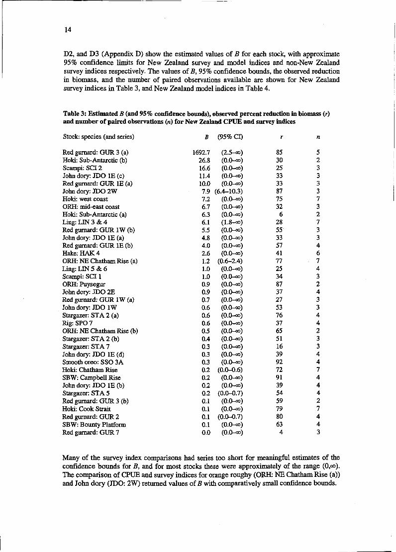
D2, and D3 (Appendix D) show the estimated values of B for each stock, with approximate 95% confidence limits for New Zealand survey and model indices and non-New Zealand survey indices respectively. The values of B, 95% confidence bounds, the observed reduction in biomass, and the number of paired observations available are shown for New Zealand survey indices in Table 3, and New Zealand model indices in Table 4.

Table 3: Estimated B (and 95% confidence bounds), observed percent reduction in biomass (r) and number of paired observations (n) for New Zealand CPUE and survey indices

Stock: species (and series) B (95% CI) r n

Red gurnard: GUR 3 (a) Hoki: Sub-Antarctic (b) Scampi: SCI 2 John dory: JDO 1E (c) Red gurnard: GUR 1E (a) John dory: JDO 2W Hoki: west coast ORH: mid-east coast Hoki: Sub-Antarctic (a) Ling: LIN 3 & 4 Red gurnard: GUR 1W (b) John dory: JDO 1E (a) Red gurnard: GUR 1E (b) Hake: HAK 4 ORH: NE Chatham Rise (a) Ling: LIN 5 & 6 Scampi: SCI 1 ORH: Puysegur John dory: JDO 2E Red gumard: GUR 1 W (a) John dory: JDO 1W Stargazer: STA 2 (a) Rig: SPO 7 ORH: NE Chatham Rise (b) Stargazer: STA 2 (b) Stargazer: STA 7 John dory: JDO 1E (d) Smooth oreo: SSO 3A Hoki: Chatham Rise SBW: Campbell Rise John dory: JDO 1E (b) Stargazer: STA 5 Red gurnard: GUR 3 (b) Hoki: Cook Strait Red gurnard: GUR 2 SBW: Bounty Platform Red gurnard: GUR 7

Many of the survey index comparisons had series too short for meaningful estimates of the confidence bounds for B, and for most stocks these were approximately of the range (0,a). The comparison of CPUE and survey indices for orange roughy (ORE NE Chatham Rise (a)) and John dory (JDO: 2W) returned values of B with comparatively small confidence bounds.

For the orange roughy stock, survey indices appeared to track the changes in survey biomass closely. The observed reduction in biomass was about 80% and 7 paired observations were available. Estimates of B suggested that a proportional relationship may be plausible, though slightly hyperstable or strong hyperdepleted relationships could not be excluded.

In the survey indices for John dory (JDO 2W), there were only three pairs of observations and the observed reduction in (observed) biomass was 87%. The estimated shape parameter was B = 8 (95% CI = 6-10), suggesting a strong hyperdepletion relationship. However, this estimate was largely determined by a single observation. (The estimator of B attempts to find a best-fit monotonic relationship between the two indices, and as biomass appears to increase with decreasing CPUE, the estimator prefers to fit a hyperdepletion relationship.)

For some stocks, although the estimated confidence bounds of B were large, they excluded the possibiity of some forms of relationship. For example, estimated B for hoki (Chatham Rise) survey indices was 0.2 (95% CI = 0-0.6), suggesting that the relationship for survey indices was most likely hyperstable, with a very low possibility of either a proportional or hyperdepletion relationship.

Table 4: Estimated B (and 95% confidence bounds), observed percent reduction in biomass (r) and number of paired observations (n) for New Zealand CPUE and model indices

Stock: Species (and series) 5 (95% CI) r n

Hake: HAK 7 (b) Hake: HAK 7 (a) Hoki: Chatham Rise Paua: PAU 5B Snapper: Hauraki Gulf / Bay of Plenty Snapper: SNA 8 (late) ORE Puysegur SBW: Bounty Platform Hake: HAK 4 ORH: Mid-east coast OW. NE Chatham Rise (a) Snapper: SNA 8 (early) Hoki: West coast Rock lobster: CRA 4 SB W: Campbell Rise Ling: LIN 3 & 4 Rock lobster: CRA 5 Smooth oreo: SSO 3A Hoki: Cook Strait ORH: NE Chatham Rise (b) Hoki: Sub-Antarctic Ling: LIN 5 & 6

Estimates of B improved when using model indices as the larger number of paired observations and greater observed reductions in estimated biomass allowed better estimates of shape. Most stocks had confidence bounds that appeared to be close to that of a proportional relationship and usually included or were between the values of 0.5 or 2.

If we assume that the model-based biomass indices provide information on B, and consider only those stocks where the confidence bounds of B suggested a monotonic relationship, then the relationship between CPUE and abundance was often close to that of a proportional

relationship. Of the 11 stocks that met the criteria of a confidence bound for B that did not include either 0 or and had reductions in observed biomass of at least SO%, 7 had confidence bounds that included 0.5 or 2. Two had confidence bounds that suggested that B was at least greater than 2, and similarly, 2 had confidence bounds that were less than 0.5. If we grouped these stocks by species, then 6 of the 9 species had confidence bounds that included 0.5 or 2. For the non-New Zealand survey indices, 2 of 3 met the criteria above and had confidence bounds that included 0.5 and 2.

However, the remaining species had bounds that suggested either no information on the relationship or suggested a relationship that was not useful for stock assessment. Very strong hyperstable relationships provide no information on the status of a stock, except to warn when catastrophic collapse has happened. Similarly, very strongly hyperdepletion relationships are useful only for determining if the stock is at or close to virgin biomass status.

The inferences that can be drawn from these data are extremely limited. The method of estimating B relies on an assumption of a structural relationship that has i.i.d. lognormal errors with constant and assumed known c.v.s. In addition, the earlier simulations suggest that the short nature of most series combined with moderate reductions in biomass prevent any strong inference on the shape of the relationship.

Although inference and generalisation based on these data should be treated with extreme caution, the results suggest that the assumption of a proportional or near proportional relationship may be adequate. The range of confidence bounds for the estimates of B suggest that values between 0.5 and 2 may encompass most relationships that might be found for a wide range of stocks or species. Hence, a possible interpretation of these results is that the assumption of proportionality may not be inadequate, although, clearly, more research on possible values of B is required. In particular, the impact of a hyperstable (B = 0.5) or hyperdepletion (B = 2) relationship on stock assessments needs to be investigated.

4. CALCULATION AND INTERPRETATION OF CPUE BY WORKING GROUPS

CPUE analyses are part of the information required by the Ministry of Fisheries for New Zealand fish stock management decisions. Ministry of Fisheries Fishery Assessment Working Groups (WGs) provide scientific advice to the Ministry of Fisheries which form the basis of these decisions. WGs are required, in part, 'To review any new research information on stock structure, productivity, and abundance and update the assessment of each Fishstock". In addition, they are specifically requested to report new information which "... alters the previous assessment, especially yield estimates and stock status.. .", and an example of such new research information given is ". . . the development of a major trend in catch or catch per unit effort" (Anriala et al. 1999).

Although WGs have occasionally used CPUE indices as a basis for stock management, they appear aware of the potential problems in their use and interpretation. We briefly review the recorded decisions of WGs as related to the use and interpretation of CPW indices. The data for this review consisted of FARDs containing stock assessment or CPUE analyses and the annual Plenary documents.

In general, WGs ,gave a variety of reasons for rejecting CPUE analyses, although the recording of decisions and rationales in FARDs and Plenary documents was sparse. Data recorded in such documents were often inadequate to determine precise reasons for rejecting individual analyses as indices of abundance. The poor recording of both the outcome of

decisions and the rationales for those decisions, and a number of apparent inconsistencies in decisions between stocks and species with similar circumstances, made summaries difficult. In particular, none of the WGs specified or mentioned a set of objective criteria by which CPUE analyses would be evaluated. Occasionally, no reasons for rejecting analyses were given in summary documents. Conversely, none of the reports explained reasons for accepting CPUE as an index of abundance.

The review of FARDs and Plenary documents found that CPUE analyses were reported for 70 fish stocks, covering 26 species. Of all analyses reported, 39 (55%) were accepted in some form as an index of abundance and 21 (30%) were rejected as they were believed to be an unreliable index of abundance. A further 10 (14%) CPUE analyses were reported, but either they were awaiting further analysis or a final decision on the use of the data had not been recorded.

Of the indices accepted as plausible indices of abundance, 10 species have had at least one stock for which the WGs accepted the CPUE indices as an index of abundance and at least one stock for which the CPUE index was rejected: 75% of the accepted indices were standardised CPUE analyses (Vignaux 1994) and the remaining 25% were unstandardised.

The criteria employed by WGs can, however, be grouped into four broad categories (see below). (In Section 6, we expand on the ideas of WGs to develop four key components in the use and interpretation of CPUE indices.)

That there is a reasonable expectation that changes in catch/effort reflect changes in abundance (i.e., the relationship between CPUE and stock abundance is believed to be such that a change in abundance will be reflected by a change in CPUE; that the changes in standardised CPUE are not believed to represent factors other than abundance).

That there was an adequate data volume free of major error (i.e., that the recorded data are an accurate reflection of catch and effort; that there are an acceptable number of records available; that there are no known major data errors or biases in catch records; that there is a low level of reporting errors; that the data contain information for most known landings).

That there was an adequate means of correcting for changes in catchability between different fishers, methods and spatial areas (i.e., that changes in fishing practice, fishing fleet, or other confounding effects can be corrected in a standardised analysis).

That the resulting CPUE indices are consistent with other, known information on abundance (i-e., no unexplained fluctuations in indices, CPUE indices are consistent with alternative, known information for the stock; that there are no other external factors that may lead to uncertainty about the ability of CPUE to index abundance).

Table 5: Reasons recorded by WGs for not using CPUE analyses in stock management

1. Ex~ectation that changes in catchleffort reflect changes in abundance Stock is believed to maintain CPUE even as abundance falls (hyperstability)

Serial depletion, with changes in abundance not reflected in CPUE (e-g., PAU (1998)) Fishing targets spawning aggregations in a small area (e.g., HOK 1E (1998), SBW (Campbell Island, 1998))

Bycatchfishery where data are believed to represent factors other than abundance Low catch rates (e.g., JDO 2E (1998)) High proportion of zero catches in catctdeffort data (e.g., JDO 2W (1998)) Distribution driven by that of an associated target species (e.g., BNS 3 (1998), HAK 7 (1998), SWA 1 (1998))

2. Adequate data volume free of maior error Inadequate records

Too few years of adequate records (e.g., LIN 5 (longline, 1997), LIN 6 (longline, 1997)) Low numbers of records (e.g., BNS 3 (1998), BNS 7 (1998), BNS 8 (1998), HAK 1 (1998)) Catch recorded explains only a small percentage of the total known landings (e.g., STA 2 (1997), STA 3 (1997)) Fishery is based in intermittent effort by most fishers (e.g., BUT) Developing fishery (e.g., SCH (1998))

Poor record keeping due to the method of recording catch and effort Catch poorly recorded as the stock is not fully in top 5 species on TCEPR forms (e.g., SWA (1999))

High level of mimeporting in catch/e&ort data Catch for some species not recorded (e.g., ELE 3 (1994), Cockles (1998))

Known data errors and bias in catch records Known problems with reporting a species or species identification errors (e.g., ELE 3 (1998)) Known species dumping (e.g., CDL 2 (1997)) Effort driven by very localised demand (e.g., RIB, BUT)

3. Adeuuate means of correcting for changes in catchability Known changes in fishing practice over time that effect CPUE

Targeting trend towards smaller catches (e.g., ORH 2 (1998)) Fishing methods change measures of catch or effort (e.g., ORH 7A (1998)) Interaction with other fisheries results in changes in fishing methods (e.g., TAR 2 (1997)) Changes in targeted species (e.g., LIN 5 (1997))

4. CPUE indices are consistent with other. known information on abundance CPUE indices are inconsistent with alternative, known information for the stock

CPUE indices not consistent with tow duration or s e k h time (e.g., BXY 2 (1996)) Inconsistent indices with expected biomass decline (e.g., ORH 3B (1991)) Fits to assessment models appear 'worse' with the addition of CPUE (e.g., ORH 7B unstandardised (1995)) Uurealistic model outputs when compared with other data (e.g.. GUR 7 (1998)) Survey index inconsistent with CPUE index (e.g., GUR 7 (1998), HOK 1W (1998), HOK 1E (1998)) Inconsistent patterns of change in CPUE across spatial areas (e.g., SPO 1 (1998), SPO 2 (1998), STA 7 (1997)) Inconsistent trends in CPUE over time (e.g., SCH (1988). SBW (Bounty Platform, 1993))

Unexplainedfluctuation in indices Index has unexplained fluctuations, and does not appear to index abundance (e.g., BNS 3 (1998) HAK 7 (1996)) .

5. Other reasons No reasons stated

ORH 7B standardised (1998), TAR 1 (1996).

5. THE CALCULATION AND INTERPRETATION OF CPUE INDICES

The calculation of CPUE does not necessarily result in an index with a useful relationship, or even any relationship, with stock abundance. It would seem sensible to attempt to calculate indices that reflect changes in abundance, and moreover have some known relationship to abundance. While this objective may often be unattainable in practice, a set of guidelines may assist in determining the level of confidence that can be placed on a set of indices. We expand on the guidelines used by WGs, to develop four components of CPUE analyses.

As a statistical analysis, the calculation of CPUE indices should ideally be considered within the general framework of statistical modelling. The stating of model assumptions, model fitting methods, and model diagnostic analyses are essential components of any statistical analysis, and should be always be applied to the analysis of CPUE data.

We develop the ad hoc guidelines derived earlier from WGs decisions, and propose that analysis of B U E should, ideally, consist of four components.

1. Determining the underlying assumptions of the catchieffort abundance rela tionship

Deciding the measures of CPUE most likely to index abundance Determining the nature of the relationship between CPUE and abundance Stating of assumptions that allow CPUE to index abundance

2. Assessment of data adequacy Determining the adequacy of the data to estimate and standardise CPUE

3. Model fitting and model validation Determining the model structure and estimating CPUE indices Determining the extent to which the model provides an appropriate description of the data

4. Evaluation of the CPUE index Validating the CPUE/abundance relationship assumption

5.f Underlying assumptions of the cstchleffort abundance relationship

The first question that should be applied to any CPUE analysis is "What is the relationship, for this fish stock, between the measures of CPUE available and abundance?WGs have considered whether an index for a particular stock would provide a useful index of abundance, but the nature of the relationship has not often been investigated. Aspects of fisher behaviour, spatial patterns in the distributions of fish, and the relationship of catchability to abundance will affect this relationship and should be considered as a part of CPUE analyses. We suggest that the analysis of CPUE should explicitly consider the relationship between CPUE and abundance as a first step. Moreover, that this consist of (a) identifying measures of CPUE that index abundance or local density, (b) determining the nature of the relationship between CPUE and abundance, and (c) the stating of any assumptions that allow CPUE to be considered an index of abundance.

This step in CPUE analysis should consider all relevant aspects of the fishery, concentrating particularly on how the fishing effort is distributed with respect to distribution of fish and relationship between fishing effort, abundance, and catchability. Both the fishing process and spatial behaviour of the fish stock need to be understood when considering this relationship.

Aggregated and non-aggregated effort measures of catch and effort could be considered, along with assumptions of changes in fishing behaviour (strategy and practice) over time and space.

As an example, consider a deepwater hill fishery that uses catch-per-kilometre as a measure of CPUE. If the fishing behaviour is to start fishing once a suitable aggregation is found, we may expect to observe a hyperstable CPWabundance relationship, and then see little change in CPUE with changing abundance. Such a measure may be useful only as an indicator of catastrophic stock collapse, rather than as a direct measure of stock size.

For a bycatch fishery, we may propose that the bycatch of a non-targeted fish could lead to a 'better' indication of abundance than targeted effort. This follows from the argument that fishing may be more randomly distributed with respect to the particular bycatch species. Unfortunately, this approach is confounded by changes in fishing practice. Fishers may actively change their fishing behaviour over time, for example, to increase bycatch when the bycatch species has high commercial value and fishers have quota remaining, or to decrease bycatch when the bycatch has little commercial value or quota is full. Langley (1995) suggested exactly such changes in fishing behaviour of the bycatch bluenose (Hyperoglyphe antarctica) fishery. Such changes in behaviour over time make the resulting interpretation of CPUE indices difficult, and indices may not even be useful as an index of gross changes in underlying biomass.

Assumptions of the relationship between CPUE and abundance will affect the interpretation of the resulting CPUE indices in stock management. More complex methods of CPUE estimation can easily be constructed, but may be less interpretable. However, the overriding concern should be to develop CPUE indices that provide a useful index of abundance, and to form ideas of how they relate to abundance. The underlying assumptions of changes in fisher behaviour and spatial distribution of fish that are needed for a calculated index to be considered an index of abundance should be stated. The exact nature of the relationship will often be unknown, and is unlikely to be estimable, although information from similar stocks or species may provide some insights.

5.2 Assessing data adequacy

Data adequacy can be thought of as encompassing two components: the ability of the data to provide an adequate sample (both temporally and spatially) of the population, and the ability of explanatory variables to allow adequate standardisation of catchability. The data should cover a reasonable time series over a well defined range of the spatial territory of the fish stock, with additional information that allows for appropriate standardisation of changes in catchability.

WGs have noted a number of reasons why catcweffort data may not be adequate (see Section 5), and have often considered data adequacy in analysis - often as a descriptive analysis (e.g., BaUara 1998, Clark 1998) or by some other form of exploratory data analysis.

An important additional consideration is the proportion of total catch from an area that is included in a particular analysis. Such information may give an indication of how representative the data and subsequently the results of a particular anaIysis are likely to be. For example, the proportion of catch in previous CPUE analyses has varied widely, from 10% of the total catch (STA2 in Vignaux 1997), to more than 80% in orange roughy trawl fisheries (M. Clark, NIWA, pers. c o r n ) .

While catchleffort data sets can be large (with hundreds or thousands of records per year), there are many reasons why catch and effort data may prove inadequate. Data quantity does not necessarily equate to data quality. For example, catches may be recorded only intermittently or a bycatch species may be caught only on the edge of its range. Variations in the composition of the fleet or other aspects of fishing practice may be impossible to disentangle from changes in CPUE caused by fluctuations in abundance.

Most data sets are not error free. CatchJeffort data are often found to have a large degree of recording and transcription error and may need extensive 'grooming' (correcting or removing records with errors). Assessments of the affects of outliers or other errors in the data can be attempted, through sensitivity analyses or other appropriate techniques. However, when data sets are large, grooming may not have much effect on final estimates of CPUE indices (see Dunn & Harley 1999 for an example), and such grooming time may be more productive when spent on better determining the means of standardisation. Examples of data grooming methods can be found in most Ministry of Fisheries reports that consider CPUE (e.g., Vignaux 1994, Ballara et al. 1998, Dunn & Harley 1999, Harley, unpublished results).

The explanatory variables that might be modelled in a CET.,R type analysis might include month or season, statistical area or region, and target species. Ballara (1998) included day-of- year to estimate seasonal trends, as well as the Southern Oscillation Index to allow for environmental affects on catch rates (both through conditions for fish and fishers). For a TCEPR type analysis it is also possible to include tow location, time of day for a tow, gear characteristics (e.g., headline height and doorspread), gear depth, and depth of bottom. For example, it may be possible to use the precise location data to model individual hill complexes. Dunn & Harley (1999) and Harley (unpublished results) determined whether an individual tow took place before, during, or after sunrise or sunset. Such a variable allows the analyst to standardise for changes in catch rates due to the diurnal or other daily change in behaviour observed in many species. In many New Zealand fisheries the number of vessels per year can range from less than 10 to over 100 @unn & Harley 1999, Harley, unpublished results). Often the physical characteristics of a particular vessel may be sufficient, but often the skills of individual skippers and crews outweigh the physical chatacteristics of the vessel (Hilborn & Walters 1992, Gaertner et al. 1998). When the number of vessels is small, it may be best to use the vessel identifier as a categorical variable, but when the number of vessels is large it may be best to use the continuous vessel data or group the vessels into a small number of classes (Vignaux 1997, Gaertner et al. 1998).

Consideration should be given to the variables unavailable for a specific analysis, particularly those that are believed to affect the relationship between CPUE and abundance but for which there are no independent measures. Most analyses reviewed for this paper did include some discussion on the adequacy of the data to fit and standardise CPUE, and examples of considerations included discussion on the level of reporting error or bias; data coverage in terms of total landings; total volume of data available for analysis; and the ability of variables to adequately standardise for variation in catchability.

Many authors have discussed the issue of increased skill or learning in fisheries (Hilbom & Walters 1992, Rose & Leggett 1993) which may result in an increase in catching power over time, regardless of changes in abundance. Most fisheries have an initial period of discovery (a learning phase), followed by more efficient fishing practice (Allen & McGlade 1986). Hence for a new fishery, it may often be prudent to disregard the first few years or seasons of a time series, or alternatively, assume a different catchability and model this as part of the standardisation.

5.3 Model fitting and model validation

Methods of model fitting to CPUE data can be viewed as methods of applied regression analysis. Not only should the analyst consider which model structures are appropriate, but also the extent to which the model provides an appropriate description of the data (Collett 1991). The investigation of systematic deviations from the assumed model fit, investigation of outliers, and tests of model assumptions are alI requirements of a statistical analysis, and hence CPUE analysis. However, few CPUE analyses reviewed for this paper present model diagnostics or other assessments of model adequacy. None attempted to analyse the residual structure as a means of understanding the model's inadequacies.

The statistical and fisheries literature on model fitting and regression methods is too vast to allow more than a quick summary of the more important points in this report. Hence, we do not review the literature on regression techniques that could be applied to CPUE analyses, but instead refer the reader to standard texts on such methods. For example, McCullagh & Nelder (1989) and Draper & Smith (1981) provided a technical statistical overview of fitting and interpreting generalised linear models, and Gavaris (1980) discussed methods of standardisation of CPUE using such regression techniques.

Raw CPUE often has a highly skewed distribution (i.e., distributed with a minority of high values), and it is often necessary to transform the data to enable an acceptable model fit. Suitable transformations suggested include the log transform (Gavaris 1980, Hilborn & Walters 1992), the square root transform (Quinn 1985), or any one of a more complex family of transformations (Bannerot & Austin 1983, Richards & Schnute 1992). More difficulties occur when the data contain zero observations (Pennington 1983, Vignaux 1994). More recently, Generalised Additive Models quasi-likelihood and pseudo-likelihood methods have been proposed that allow more computer intensive methods of fitting complex spatial or temporal variations in the effort.

Catchability is likely to differ across different parts of the fishery. For example different locations, different vessels, or seasonal fish behaviour may have characteristics that result in different catching power (Gavaris 1980, Hilbom & Walters 1992). At the very least, the spatial variation in the data should be investigated (Hilbom & Walters 1992), and some consideration given to seasonal fluctuations and changes in fishing fleet composition.

The usual method of standardisation of catchleffort data is that of Gavaris (1980), in which the ratio of catchleffort is modelled as a function of some index of abundance, with explanatory variables used to standardise for differences in catchability. Alternative methods have been suggested: for example, Woahington et al. (1998) modelled catch as function of effort and abundance, standardising for other explanatory variables in the usual manner.

Abrupt changes in fleet structure or timing and location of fishing can be difficult to standardise within an analysis. Short term changes in such components can easily be confounded with calculated yearly indices, giving CPUE estimates that may index changes in fishing practice rather than abundance. Under such changing circumstances it may be necessary to analyse only a subgroup of the data, whether it be a season or region or a specific group of vessels. Tbis relates back to the earlier point, that CPUE indices will contain information only on the subset of the fish stock actually fished. Sometimes, it may be necessary to have two separate series, as for smooth ore0 in 3A (Doonan et al. 1998).

Vignaux (1994) used the approach of Gavaris (1980) in combination with a stepwise regression approach based on maximising the ratio of residual deviance to null deviance with an appropriate stopping rule. Most statistical texts warn away from automatic variable selection in regression approaches as a form of statistical modelling, but this is a minor point in that the primary goal of CPUE analyses is not to provide a parsimonious explanatory model of CPUE, but is an exercise in determining an abundance index. Problems of automatic variable analysis in regression that have been reported in the statistical literature suggest that estimated confidence intervals are too narrow (Altman & Andersen 1989), 3 values are biased high, F statistics may be unreliable, and reported regression coefficients can be biased (Tibshirani 1996).

Key points that should be considered during analysis include model selection and distributional assumptions, methods of standardisation, the inclusion of confounding factors and interaction terms, the interpretation of parameters, assessments of model goodness-of-fit, checking distributional assumptions, diagnostic analysis of residuals, and identification of outliers.

5.4 Evaluation of CPUE indices

As noted earlier, the calculation of a CPUE index does not, in itself, imply that a relationship exists between the resulting index and stock abundance. The use and interpretation of a specific CPUE index should depend on a careful evaluation on how or whether it indexes abundance. Validation of calculated indices asks the question 'What information allows us to either confirm or reject the CPUE index as an index of abundance?'It should be noted that the evaluation of CPUE indices differs from model evaluation. The latter uses the data available to the regression model to investigate departures from model assumptions, and is essentially concerned with model consistency. Evaluation of CPUE indices uses information from outside this process to verify that the resulting indices index abundance.

In general, validation of an index is rarely explored as part of the analysis, partly because, while methods for such comparison are available, data inadequacies mean that they are often unsatisfactory. The best method for checking and validating a CPUE index is comparison with other abundance information. However, this is difficult when little accurate alternative information is available. Where the alternative abundance information exists, direct comparison of CPUE with non-CPUE indices directly are implemented. Model estimates of abundance may allow a better comparison, but rely on the assumptions contained within the stock model. Even if comparison is practical, issues relating to gear selectivity, age based selectivity, and the relative availability of the exploitable population may dominate any comparison.

An indication of the appropriateness of a particular model will be the consistency in the explanatory variables fiom year to year. For some fish stocks, for example, deepwater stocks, there may be an expectation that the main variables should remain consistent over time - if they have substantial unexplained variation, then the acceptance of the analysis may be limited (M. Clark, pers. c o r n ) .

Alternative, associated data such as length or age frequencies, relative recruitment or year class strength estimates, quota overruns, landings statistics, or records of fisher perceptions may allow some qualitative comparison. For example, Knuckey et al. (unpublished results) compared CPUE fiom two similar stocks of silver warehou (Seriolella punctata). They noted that the similarities between the two series, in conjunction with peaks in CPUE that corresponded to peaks in length frequency data (and believed to be indicative of high

recruitment) in similar years, supported the conclusion that CPUE indexed abundance for both stocks.

Trends in catching ability also need some consideration, as technological and scientific advances as well as changes in fishing practice can contribute to changes in catch over time (an effect that may not be able to be disentangled from trends in abundance). Further problems arise when considering spawning stocks, migratory species, or other similar fish stock and fisher behaviours. CPUE indices will contain only information on the subset of the fish stock actually fished, and hence any relationship between CPUE and abundance will only be a reflection of the proportion of the fish stock that was sampled by the related fishing activity (effort).

6. DISCUSSION

It is often useful to assume that changes in CPUE will, to some extent, reflect changes in stock abundance. This is a convenient assumption for those managing fish stocks, but it must be noted that this assumption cannot often be tested and may be inadequate. Hilbom & Walters (1992) warned "It is simply irresistible to try to use CPUE data to estimate an index of abundance." If a proportional relationship is unlikely, a monotonically increasing functional relationship of some sort may be a better (and weaker) assumption.

Should we reject the idea of a proportional relationship between CPUE and abundance? A proportional relationship between CPUE and abundance may be strictly incorrect, but it is possible that such an assumption may still be a reasonable approximation. Clearly, as long as we can be satisfied that the relationship between CPUE and abundance is not too far from proportional, it may still provide useful information for stock assessment. However, the effects of other relationships on stock assessment models have yet to be investigated.

Empirical investigation earlier suggested that the relationship between CPUE and abundance can be described by a simple shape parameter, B. Estimated values for B appeared to always include values between 0.5 and 2.0, suggesting possible sensitivity bounds for CPUE abundance relationships in stock assessments. In addition, many stocks had values of B close to 1, suggesting that a proportional relationship might be an adequate approximation for some stocks. However, the investigation into possible shapes of the relationship between CPUE and abundance relies on strong assumptions, and should be considered with some caution.

Simulations suggest that only when a large amount of data is available and when a substantial reduction in true biomass has occurred will it be possible to estimate, even approximately, the shape of the relationship between CPUE and biomass. Further research is required on the values of B that provide some information for stock assessment models, the effect of a non- proportional relationship on estimates of biomass, or the robustness of stock assessment models to a non-proportional relationship between CPUE and abundance.

Where the relationship between CPUE and abundance is known to be strongly non- proportional, CPUE may still be a useful, though limited, stock management tool. For example, where the relationship is hown to be strongly hyperstable, CPUE may assist in determining whether a stock is close to catastrophic collapse.

Many of the CPUE analyses reviewed for this report did not appear to have been evaluated against an objective set of criteria. Appropriate stock management using CPUE indices relies on assessments of data accuracy and assumptions of relationships between CPUE and abundance. Few analyses attempted to quantify either of these aspects. However, WGs have

developed a number of informal rules-of-thumb for using, calculating, and interpreting CPUE indices. Unfortunately, these appear to be poorly implemented and lack consistency between stocks and analyses.

We have developed these guidelines into a list of four components. We recommend that CPUE analyses include discussion of these as a part of standard analysis. These components are

1. Definition of the relationship between CPUE and abundance 2. Assessment of data adequacy 3. Methods of model fitting and model validation 4. Evaluation of the CPUE index

It is clear that there are no comprehensive means for evaluating CPUE indices, even when appropriate steps have been taken in the analysis of catchleffort data. Simply put, there are no easy answers, and every analysis requires a good understanding of both the fishery and the factors that can influence the CPWabundance relationship. Even so, there remains the question of whether CPUE does index abundance for a particular fish stock Although the likelihood of an approximate proportional relationship between CPUE and abundance seems good, without validation CPUE indices should be considered suspect and used only with caution in any analysis of stock status.

7. ACKNOWLEDGMENTS

We thank the many NIWA personnel who contributed to the detail of this paper, and others who assisted through numerous discussions and conversations with the authors. We thank Patrick Cordue for his comments and the improvements that resulted from his review of this paper. This research was funded by the Ministry of Fisheries under Project SAM 9801.

8. REFERENCES

Allen, P.M. & McGlade, J.M. 1986: Dynamics of discovery and exploitation: The case of the Scotian Shelf groundfish fisheries. Canadian Journd of Fisheries and Aquatic Sciences 43(5): 1 187-1200.

Altman, D.G. & Andersen, P.K. 1989: Bootstrap investigation of the stability of a Cox regression model. Statistics in Medicine 8: 771-783.

Angelsen, K.K. & Olsen, S. 1987: Impact of fish density and effort level on catching efficiency of fishing gear. Fisheries Research 5: 271-278.

Annala, J.H., Sullivan, K.J., & O'Brien, C.J. (Comps.) 1999: Report from the Fishery Assessment Plenary, April 1999: stock assessments and yield estimates. 430 p. (Unpublished report held in NIWA library, Wellington).

Annala, J.H., Sullivan, K.J., OBrien, C.J., & Iball, S.D. (Comps.) 1998: Report fiom the Fishery Assessment Plenary, May 1998: stock assessments and yieId estimates. 409 p. (Unpublished report held in NIWA library, Wellington).

Arreguin-Shchez, F. 1996: Catchability: a key parameter in stock assessment. Reviews in Fish Biology 6(2): 221-242.

Ballara, S.L. 1998: Hoki non spawning CPUE feasibility. Final Research Report to the Ministry of Fisheries. Project HOK 9701 (Objective 2). 21 p.

Ballara, S.L., Cordue, P.L., & Livingston, M.E. 1998: A review of the 1996-97 hoki fishery and assessment of hoki stocks for 1998. N.Z. Fisheries Assessment Research Document 98125.58 p. (Unpublished report held in NlWA library, Wellington).

Bannerot, S.P. & Austin, C.B. 1983: Using frequency distributions of catch per unit effort to measure fish-stock abundance. Transactions of the American Fisheries Society 112(5): 608-617.

Baranov, T.I. 1918: K voprosu o biologicheskii osonvaniiak. rybnova khoziaistva. [On the question of the biological basis of fisheries. Translation by Ricker, W.E., Indiana University, Indiana, 19451. Nauchnyi issledovatelskii iktiologisheskii Institut, Izvestiia l(1): 8 1-128.

Bishir, J. & Lancia, R.A. 1996: On catch-effort methods of estimating animal abundance. Biometrics 52: 1457-1466.

Breen, P.A. & Kendrick, T.H. 1999: Rock lobster stock assessment for CRA 3, CRA 4, and CRA 5 in 1998. N.Z. Fisheries Assessment Research Document 99/35. 55 p. (Unpublished report held in NIWA library, Wellington).

Clark, S.H. (Ed.) 1998: Status of fishery resources off the Northeastern United States for 1998. NAOO Technical Memorandum NMFS-NE-155. NAOO, Woods Hole, Massachusetts.

Collett, D. 1991: Modelling binary data. Chapman and Hall, London. 369 p.

Cooke, J.G. 1985: On the relationship between catch per unit effort and whale abundance. Report of the International Whaling Commission 35: 5 1 1-5 19.

Cordue, P.L. 1999: MIAEL estimation of biomass and fishery indicators for the 1998 assessment of hoki stocks. N.Z. Fisheries Assessment Research Document 9911.64 p. (Unpublished report held in NIWA library, Wellington).

Crecco, V. & Overholtz, W.J. 1990: Causes of densitydependent catchability for Georges Bank haddock Melanogrammus aeglefinus. Canadian Journal of Fisheries and Aquatic Sciences 47(2): 385-394.

Csirke, J. 1988: Small shoaling pelagic fish stocks. In: Fish population dynamics: the implications for management. 2nd edition edition. Gulland, J.A. (Ed.) 271-302. John Wiley & Sons, London.

Davies, N.M. 1997: Assessment of the west coast snapper (Pagnss auratus) stock (SNA 8) for the 1996-97 fishing year. N.Z. Fisheries Assessment Research Document 97112. 18 p. (Unpublished report held in NIWA library, Wellington).

deLury, D.B. 1947: On the estimation of biological populations. Biometrics 3: 145-167.

Doonan, I.J., Coombs, R.F., McMillan, P.J., & Dunn, A. 1998: Estimate of the absolute abundance of black and smooth ore0 in OEO 3A and 4 on the Chatham Rise. Final Research Report to the Ministry of Fisheries Project OEO 9701.46 p.

Doonan, I.J., McMillan, P.J., Coburn, R., & Hart, A.C. 1997: Assessment of Chatham Rise smooth ore0 (OEO 3A and OEO 4) for 1997. N.Z. Fisheries Assessment Research Document 9712 1.26 p. (Unpublished report held in NIWA library, Wellington).

Draper, N.R. & Smith, H. 1981: Applied regression analysis. 2nd edition. Wiley, New York 709 p.

Dunn, A. 1998: Stock assessment of hake (Merluccius australis) for the 1998-99 fishing year. N.Z. Fisheries Assessment Research Document 98/30. 19 p. (Unpublished report held in MWA library, Wellington).

Dunn, A. & Doonan, I. 1997: Investigations into the relationship between catch per unit effort (CPUE) and fish abundance. Final Research Report to the Ministry of Fisheries Project FMFMO1. 16 p.

Dunn, A. & Harley, S.J. 1999: Catch-per-uniteffort (CPUE) analysis of the non-spawning hoki (Macmronus novaezelandiae) fisheries on the Chatham Rise for 1989-90 to 1997-98 and the Sub-Antarctic for 1990-91 to 1997-98. N.Z. Fisheries Assessment Research Document 99/50. 19 p. (Unpublished report held in NIWA library, Wellington).

Gaertner, D., Pagavino, M., & Marcano, J. 1998: Influence of fishers' behaviour on the catchability of surface tuna schools in the Venezuelan purse-seiner fishery in the Caribbean Sea. Canadian Joumal of Fisheries and Aquatic Sciences 56(3): 394-406.

Gavaris, S. 1980: Use of a multiplicative model to estimate catch rate and effort from commercial data. Canadian Journal of Fisheries and Aquatic Sciences 37(12): 2272-2275.

Gillis, D.M., Peterman, R.M., & Tyler, A.V. 1993: Movement dynamics in a fishery: Application of the ideal free distribution to spatial allocation of effort. Canadian Journal of Fisheries and Aquatic Sciences 50(2): 323-333.

Gordoa, A. & Hightower, J.E. 1991: Changes in catchabiity in a bottom-trawl fishery for Cape hake (Merluccius capensis). Canadian Journal of Fisheries and Aquatic Sciences 48(lO): 1887-1895.

Hanchet, S.M. 1997: Southern blue whiting stock assessment for the 1996-97 and 1997-98 fishing year. N.Z. Fisheries Assessment Research Document 97/14. 32 p. (Unpublished report held in NIWA Library, Wellington).

Harley, S.J. 1999: Catch per unit effort (CPUE) analysis of the Chatham Rise, Southern Plateau, and Bounty Plateau ling (Genyptems blacodes) longline fisheries. N.Z. Fisheries Assessment Research Document 99/31. 26 p. (Unpublished report held in NIWA library, Wellington).

Hilborn, R. 1985: Fleet dynamics and individual variation: why some people catch more fish than others. Canadian Jouml of Fisheries and Aquatic Sciences 42(1): 2-13.

Hilborn, R. & Walters, C.J. 1987: A general model for simulation of stock and fleet dynamics in spatially heterogeneous fisheries. Canadian Journal of Fisheries and Aquatic Sciences 44: 1366-1369.

Hilbom, R. & Walters, C.J. 1992: Quantitative fisheries stock assessment. Choice, dynamics and uncertainty. Chapman and Hall, New York. 570 p.

Horn, P.L., Hanchet, S.M., Stevenson, M.L., Kendrick, T.H., & Paul, L.J. 1999: Catch history, CPUE analysis, and stock assessment of John dory (Zeus faber) around the North Island (Fishstocks JDO 1 and JDO 2). N.Z. Fisheries Assessment Research Document 99133.58 p. (Unpublished report held in NIWA library, Wellington).

Kendall, M. & Stuart, A. 1967: Kendall's advanced theory of statistics, Volume II. 3rd edition. Charles Griffin & Co, London. 690 p.

Kendrick, T.H. 1998: Feasibility of using CPUE as an index of stock abundance for hake. N.Z. Fisheries Assessment Research Document 98/27. 22 p. (Unpublished report held in NIWA library, Wellington).

Langley, A.D. 1995: Analysis of commercial catch and effort data from the QMA 2 alfonsino-bluenose trawl fishery, 1989-94. N.Z. Fisheries Assessment Research Document 95/18. 13 p. (Unpublished report held in NIWA library, Wellington).

MathSoft 1997: S-PLUS Users Guide. Data Analysis Products Division, MathSoft, Seattle WA.

McCall, A.D. 1976: Density dependence of catchability coefficient in the California Pacific sardine Sardinops sagax caenrlea, purse seine fishery. Californian Cooperative of Fisheries Investors Reports 18: 136-148.

McCullagh, P. & Nelder, J.A. 1989: Generalized linear models. 2nd edition. Chapman and Hall, London. 5 11 p.

Paloheimo, J.E. & Dickie, L.M. 1963: Abundance and fishing success. Contributions to Symposium 1963, on measurement of abundance of fish stocks, Copenhague. Gulland, J.A. (Ed.) Vol 155: 152-163. Conseil Permanent International pour 1'Exploration de la Mer.

Pennington, M. 1983: Efficient estimators of abundance, for fish and plankton surveys. Biometrics 39(1): 28 1-286.

Peterman, R.M. & Steer, G.J. 1981: Relation between sport-fishing catchability coefficients and salmon abundance. Transactions of the American Fisheries Society 110(5): 585-593.

Quinn, T.J. 1985: Catch-per-uniteffort: a statistical model for the Pacific halibut (Hippoglossus stenolepis). Canadian Jouml of Fisheries and Aquatic Sciences 42: 1423-1429.

Quinn, T.J. 1987: Standardisation of catch per unit of effort for short-term trends in catchability. Natural Resource Modelling 1: 279-296.

Richards, L.J. & Schnute, J.T. 1986: An experimental and statistical approach to the question: is CPUE an index of abundance. Canadian Journal of Fisheries and Aquatic Sciences 43: 1214-1227.

Richards, L.J. & Schnute, J.T. 1992: Statistical models for estimating CPUE from catch and effort data. Canadian Journal of Fisheries and Aquatic Sciences 49(7): 13 15-1 327.

Rose, G.A. & Leggett, W.C. 1991: Effects of biomass-range interactions on catchability of migratory demersal fish by mobile fisheries: An example of Atlantic cod (Gadus morhua). Canadian Jounzal of Fisheries and Aquatic Sciences 48(5): 843-848.

Rose, G.A. & Leggett, W.C. 1993: Use of oceanographic forecasts and echosounders to guide and enhance an inshore gillnet fishery for Atlantic cod (Gadus morhua). Canadian Journal of Fisheries and Aquatic Sciences 50(10): 2129-2136.

SalazarHermoso, F. & VillavicencioGarayzar, C. 1999: Relative abundance of the shovelnose guitarfish Rhinobatos productus (Ayres, 1856) (Pisces: Rhinobatidae) in Bahla Almejas, Baja California Sur, from 1991 to 1995. Ciencias Marinas 25(3): 401-422.

Seber, G.A.F. 1982: The estimation of animal abundance and related parameters. MacMillan Publishing, New York 654 p.

Swain, D.P. & Sinclair, A.F. 1994: Fish distribution and catchability: What is the appropriate measure of distribution? Canadian Journal of Fisheries and Aquatic Sciences 51(5): 1046-1054.

Tibshirani, R. 1996: Regression shrinkage and selection via the lasso. Journal of the Royal Statistical Society Series B 58: 267-288.

Ulltang, 0. 1976: Catch per unit effort in the Norwegian purse seine fishery for Alanto- Scandinavian herring. FA0 Technical Report 155.91-101 p.

Vignaux, M. 1994: Catch per unit effort (CPUE) analysis of west coast South Island and Cook Strait spawning hoki fisheries, 1987-93. N.Z. Fisheries Assessment Research Document 9411 1.29 p. (Unpublished report held in NIWA library, Wellington).

Vignaux, M. 1996: Analysis of vessel movements and strategies using commercial catch and effort data from the New Zealand hoki fishery. Canadian Journal of Fisheries and Aquatic Sciences 53(9): 2126-2136.

Vignaux, M. 1997: CPUE analysis for fishstocks in the adaptive management programme. N.Z. Fisheries Assessment Research Document 97124.68 p. (Unpublished report held in NIWA library, Wellington).

Worthington, D.G., Andrew, N.L., & Bentley, N. 1998: Improved indices of catch rate in the fishery for blacklip abalone, Haliotis rubra, in New South Wales, Australia. Fisheries Research 36: 87-97.

APPENDIX A: STOCKS, DATA, AND DATA SOURCES FOR NEW ZEALAND AND NON-NEW ZEALAND ABUNDANCE INDICES

Table Al : New Zealand fish species, stocks and abundance indices

Species Stock

Hake HAK 4

HAK 7

West Coast

Sub-Antarctic

Hoki

Cook Strait

Chatham Rise

John dory JDO 1E

JDO lW

JDO 2E

JDO 2W

Index

CPUE Survey Model CPUE CPUE Model CPUE Survey Model CPUE Survey Survey Model CPUE Survey Model CPUE Survey Model CPUE CPUE Survey Survey CPUE Survey CPUE Survey CPUE Survey

Source

TCEPR Trawl MIAEL TCEPR TCEPR MIAEL TCEPR Acoustic MIAEL TCEPR Trawl Trawl MAEL TCEPR Acoustic MAEL TCEPR Trawl MIAEL CELR CELR Trawl Trawl CELR Trawl CELR Trawl CELR Trawl

Data methodhessel

Target HAK trawl Tangaroa UQ Target hake Hake or hoki trawl UQ Target (spawning) Tangaroa LSQ Target (non-spawning) Southern Plateau @ec) Southern Plateau (April) LSQ Target (spawning) Kaharoa LSQ Target (non-spawning) Tangaroa (5+) LSQ Bycatch trawl (linear) Bycatch D. seine (linear) Kaharoa BOP Kaharoa Hauraki Gulf Bycatch trawl (linear) Kaharoa WCNI (QMA 9) Bycatch trawl (comb) Kaharoa ECNI Bycatch trawl (comb) Kaharoa WCNI (QMA 8)

Reference

(Kendrick 1998) (Dunn 1998) (Dunn 1998) (Kendrick 1998) (Kendrick 1998) (Dunn 1998) (Ballara et al. 1998) (Annala et al. 1998) (Cordue 1999) (Dunn & Harley 1999) (Annala et al. 1998) (Annala et al. 1998) (Cordue 1999) (Ballara et al. 1998) (Annala et al. 1998) (Cordue 1999) (Dunn & Harley 1999) (Annala et al. 1998) (Cordue 1999) (Horn et al. 1999) (Horn et al. 1999) (Annala et al. 1998) (Annala et al. 1998) (Horn et al. 1999) (Annala et al. 1998) (Horn et al. 1999) (Annala et al. 1998) (Horn et al. 1999) (Annala et al. 1998)

Table A1 (continued): New Zealand fish species, stocks and abundance indices

Species Stock

Ling LIN 3'94

LIN 5&6

Red gurnard GUR 7

GUR 3

GUR 1E

GUR 1W

GUR 2

Rig SPO 7 Orange roughy Mid-east coast

NE Chatham Rise

Puysegur

Index

CPUE Survey Model CPUE Survey CPUE Model CPUE Survey CPUE Survey Survey CPUE Survey Survey CPUE Survey Survey CPUE Survey CPUE CPUE Survey Model CPUE CPUE Survey Model CPUE Survey Survey Model

Source

CELR Trawl Pmod CELR Trawl TCEPR Pmod CELR Trawl CELR Trawl Trawl CELR Trawl Trawl CELR Trawl Trawl CELR Trawl CELR TCEPR Trawl Pmod TCEPR TCEPR Trawl Pmod TCEPR Trawl Trawl Pmod

Data method/vessel

Target LIN line Tangaroa (Chatham Rise) LsQ Sub-Antarctic Tangaroa (StewartISnares) Puysegur (box) LSQ flatfish trawl (comb) Kaharoa WCSI Trawl (catches + target) Kaharoa ECSI (winter) Kaharoa ECSI (summer) Bycatch trawl (comb) Kaharoa BOP Kaharoa Hauraki Gulf Bycatch trawl (comb) Kaharoa WCNI (QMA 9) ~aharoa WCM (QMA 8) Bycatch trawl (comb) Kaharoa ECNI Target set net ' Target trawl Tangaroa UQ Target trawl Target trawl Tangaroa UQ Target trawl Will WatcWGiljanes Tangaroa UQ

Reference

(Harley 1999) (Annala et al. 1998) (Bull, unpublished analysis) (Harley 1999) (Annala et al. 1998) (Annala et al. 1998) (Bull, unpublished analysis) (Annala et al. 1998) (Annala et al. 1998) (Vignaux 1997) (Vignaux 1997) (Vignaux 1997) (Hanchet et al. Unpublished results) (Annala et al. 1998) (Annala et al. 1998) (Hanchet et al. Unpublished results) (Annala et al. 1998) (Annala et al. 1998) (Hanchet et al. Unpublished results) (Annala et al. 1998) (Annala et al. 1998) (Annala et al. 1998) (Annala et al. 1998) (Bull, unpublished analysis) (Bull, unpublished analysis) (Bull, unpublished analysis) (Annala et al. 1998) (Bull, unpublished analysis) (Annala et al. 1998) (Annala et al. 1998) (Annala et al. 1998) (Bull, unpublished analysis)

Table A1 (continued): New Zealand fish species, stocks and abundance indices

Species

Scampi

Southern Blue Whiting

Stargazer

Snapper

Smooth ore0

Rock lobster

Paua

Stock

SCI 1

SCI 2

Campbell Rise

Bounty Platform

STA 2 STA 2 STA 2 STA 5 STA 5 STA 7 STA 7 SNA 8 (early)

SNA 8 (late)

Hauraki Gulf / Bay of Plenty

SSO 3A

CRA 4

CRA 5

PAU 5B

Index

CPUE Survey CPUE Survey CPUE Survey Model CPUE Survey Model CPUE Survey Survey CPUE Survey CPUE Survey CPUE Model CPUE Model CPUE Model CPUE Survey Model CPUE Model CPUE Model CPUE Model

Source

Trawl

TCEPR acoustics SPA TCEPR acoustics SPA CELR Trawl Trawl CELR Trawl CELR Trawl CELR Catch-at-age CELR Catch-at-age CELR Catch-at-age TCEPR trawl Pmod CELR Catch-at-age CELR Catch-at-age CELR Catch-at-age

Data methodfvessel

Tangaroa

Tangaroa Target trawl Tangaroa

Target trawl Tangaroa

B ycatch trawl (comb) ECNI trawl (inshore) ECNI trawl (scampi) Target trawl (comb) StewartJSnares Bycatch trawl (comb) WCSI Target pair trawls Max. Lik. Target pair trawls Max. Lik. Target trawl Max. Lik. Target trawl Tangaroa UQ Daily catch Max. Lik. Daily catch Max. Lik. Daily catch Max. Lik.

Reference

(Annala et al. 1998) (Annala et al. 1998) (Annala et al. 1998) (Annala et al. 1998) (Hanchet 1997) (Hanchet 1997) (Hanchet 1997) (Bull, unpublished analysis) (Hanchet 1997) (Hanchet 1997) (Vignaux 1997) (Vignaux 1997) (Vignaux 1997) (Vignaux 1997) (Vignaux 1997) (Vignaux 1997) (Vignaux 1997) (Davies 1997) (Davies 1997) (Davies 1997) (Davies 1997) (Field, K. pers. comm.) (Gilbert, D. pers. comrn.) (Doonan et al. 1997) (Annala et al. 1998) (Bull, unpublished analysis) (Breen & Kendrick 1999) (Breen & Kendrick 1999) (Breen & Kendrick 1999) (Breen & Kendrick 1999) (Breen et al., unpublished results) (Breen et al., unpublished results)

Table A2: Non-New Zealand fiih species, stocks and abundance indices

Species

Scallops Scallops Scallops Shrimp Shrimp Winter flounder Winter flounder Atlantic salmon Atlantic salmon Redfish Redfish Redfish Redfish Redfish Redfish Capelin Capelin Capelin Capelin Capelin Halibut Halibut Halibut

Stock

Nova Scotia Nova Scotia Nova Scotia Newfoundland (HC + 3k) Newfoundland (HC + 3k) Nova Scotia (4X) Nova Scotia (4X) Campbellton River Campbellton River Laurentian Channel Laurentian Channel Laurentian Channel Division 3 0 Division 3 0 Division 3 0 Newfoundland (3L) Newfoundland (3L) Newfoundland (3L) Newfoundland (2J3K) Newfoundland (2J3K) Nova Scotia (4VWX) Nova Scotia (4VWX) Nova Scotia (4VWX)

Index

CPUE CPUE Survey CPUE Survey CPUE Survey CPUE Survey CPUE Survey Survey CPUE Survey Survey Survey Survey CPUE CPUE Survey CPUE Survey Survey

Source

Logbook Logbook Trawl Trawl Trawl Trawl Trawl Recreational Counts

Trawl Trawl Canadian Trawl Trawl Trawl Acoustic Purse seine USSR Acoustic Longline Trawl Trawl

Data method

kglhour kglcrhm Ages 4-8 (standardised) kglhour Survey Standardised Survey Survey 'Small' fish Standardised Jan-Feb survey Apr-May survey Standardised Spring survey Autumn survey Bycatch (%) Canadian survey Unstandardised Unstandardised Canadian survey Target Summer survey Spring survey

CSASRD Report No. 98/69 CSASRD Report No. 98169 CSASRD Report No. 98169 CSASRD Report No. 98ff 2 CSASRD Report No. 98ff 2 CSASRD Report No. 971105 CSASRD Report No. 971105 CSASRD Report No. 981103 CSASRD Report No. 981103 CSASRD Report No. 9711 13 CSASRD Report No. 9711 13 CSASRD Report No. 9711 13 CSASRD Report No. 9711 15 CSASRD Report No. 9711 15 CSASRD Report No. 9711 15 DFO AFRD Report No. 95/70 DFO AFRD Report No. 95170 DFO AFRD Report No. 95170 DFO AFRD Report No. 95/70 DFO AFRD Report No. 95/70 DFO AFRD Report No. 95/44 DFO AFRD Report No. 95144 DFO AFRD Report No. 95144

Table A2 (continued): Non-New Zealand fish species, stocks and abundance indices

Species Stock Index Source Data method Reference*

White hake Nova Scotia (4 & 5) CPUE All gear Standardised CSASRD Report No.. 981143 White hake Nova Scotia (4 & 5) Survey Trawl Summer (4V) survey CSASRD Report No. 981143 White hake Nova Scotia (4 & 5) Survey Trawl Summer (4X) survey CSASRD Report No. 981143 White hake Nova Scotia (4 & 5) Survey Trawl March (Georges Bank) survey CSASRD Report No. 981143 White hake Nova Scotia (4 & 5) Survey Trawl Spring (4VsW cod) survey CSASRD Report No. 981143

CSASRD refers to the Canadian Stock Assessment Secretariat Research Documents published by the Department of Fisheries and Oceans, Canada. DFO AFRD refers to the DFO Atlantic Fisheries Research Document, published by the Department of Fisheries and Oceans, Canada.

APPENDIX B: PLOTS OF CPUE AND NON-CPUE INDICES FOR NEW ZEALAND AND NON-NEW ZEALAND FISH STOCKS

Hake: HAK 4

"I Hold: West Coast

John dory: JDO 1 E @) Hoki: Cock Strait

I H&: Chatham Rise I

John dory: JDO 1E (a) I

srvg: T d (Ksharoa BOP)

John dory: JDO 1 E (c)

. -- . -,>. 1 John dory: J W 1E (d)

I John dory: JDO 1 W

John dory: JDO 2W q - q Red gumard: GUR 7

Red gumard: GUR 3 @) Red gumard: GUR 1E (a) Red gurnard: GUR 1E (b)

Y #

Figure B1: Plots of CPUE and survey indices for New Zealand fish stocks.

Red gumard: GUR 1W (a)

ORH: Mideast coast

I

Scampi: XI 1

3 8 P

w r . STA 2 (a)

Smooth om: SS0 3A

Red gumard: GUR 1W (b)

C . - . . . . . ',

ORH: NE Chatham Rise (a)

I

mazer: STA 2 (b)

I

Red gumard: GUR 2

ORH: NE Chatham Rise (b)

SEW: Campbell Rise

Stargazer: STA5

ORH: Puysegur

7

SBW: Baunly Pl;mm

Stargazer: STA 7

. I 1 I

%

F i e B1 (continued): Plots of CPUE and survey indices for New Zealand fish stocks.

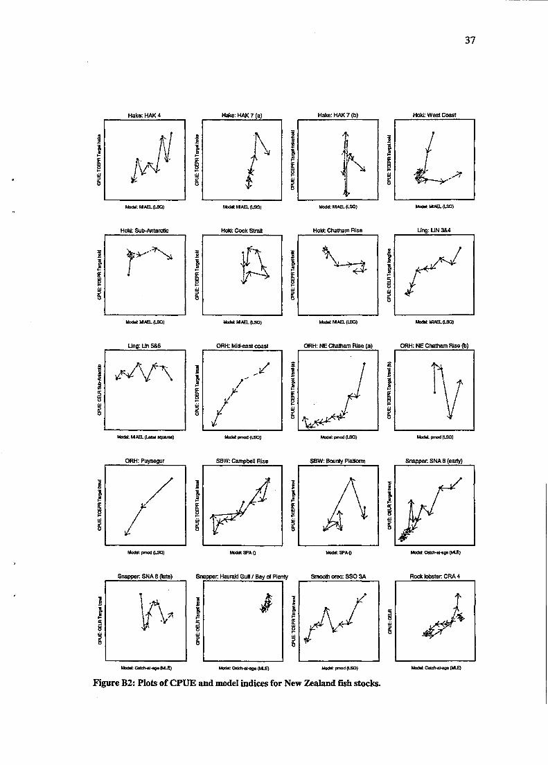
Hake: HAK 4

i !2 !2 %

Hake: HAK 7 (a)

f V

Hake: HAK 7 (b)

Hoki: Sub-Antardic I

Hdd: Cook Strait

I Hola': Chatham Rise

-M=(Lso)

ORH: Mideast wast Ung: Lin 586 ORH: NE Chatham Rise (a)

Snapper: SNA 8 (earfy)

1 j i3

Snapper: SNA 8 (late) Snapper: Hauraki Gulf 1 Bay of Pleni Rock lobster: CRA 4

7

F i e B2: Plots of CPUE and model indices for New Zealand fsh stocks.

Rock lobster: CRA 5

F i e B2 (continued): Plots of CPUE and model indices for New Zealand fish stocks.

Scellms: N w a Scotia (a) Scallops: N w a -a @) - rimp: Newfwndbnd (HC B 3k)

;. Winter flounder: N w a SW'a I 4 a

R&& Lawentian Channel (a) Redfish: Laurenthn Channel @) Redfish. D N ~ s ~ 30 (a)

I

Redfish: Division 30 @) Capelin: Newfwndland (3L) (a) Capelin: Newfoundland (3L) @)

a

abut Nova ScaSa (4VWX) (a Haakh Nwa S d a (4VWXl It White Hake: Nwa Scolia I4 a 5) la) White Hake: Nwa Scotia I4 8 51 b)

W W Hake: N w a Sartia (4 8 5) (c) White Hake: Nwa Scotia (4 8 5) (d)

I m

Figure B3: Plots of CPUE and non-CPUE indices for non-New Zealand fish stocks.

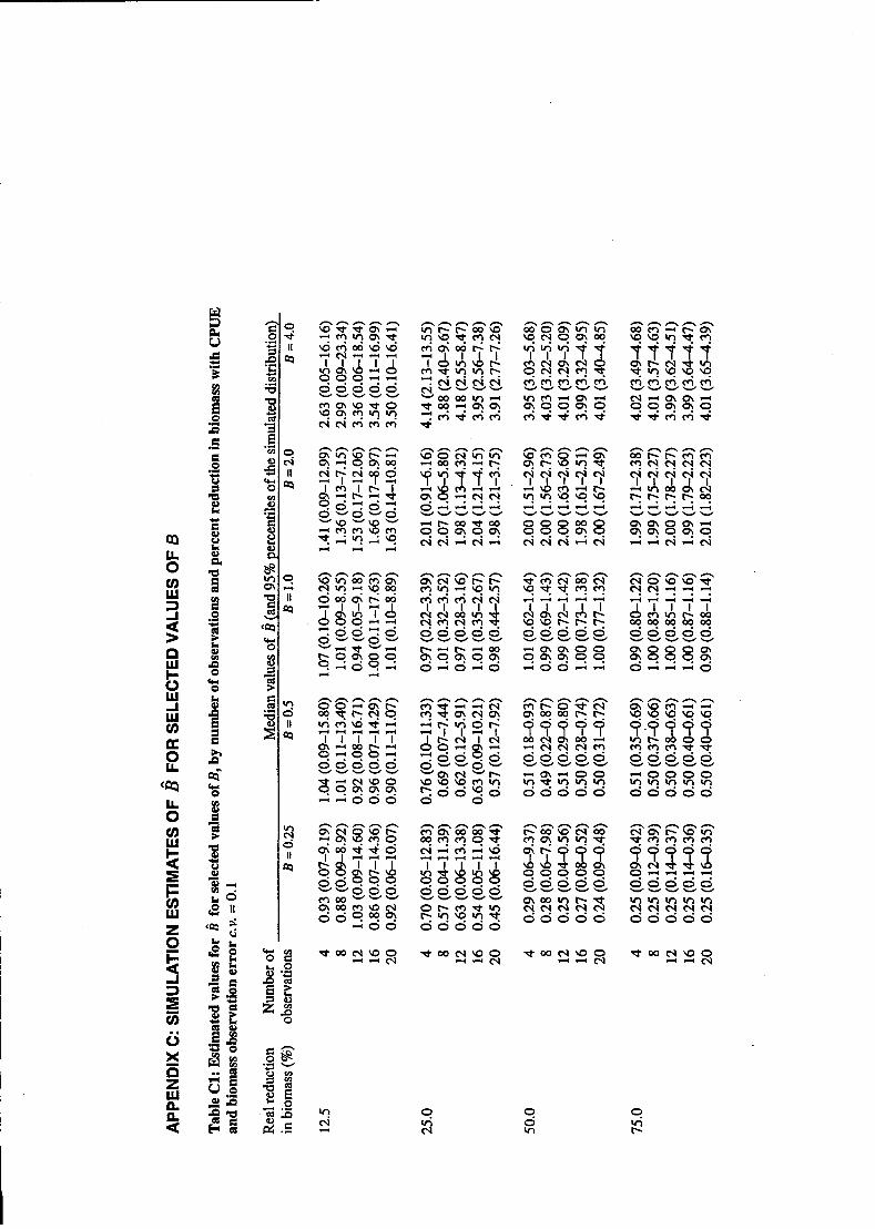
nnnnn w m o - c h 22!22 I I A d A - e

nnnnn s3s::z I I I I I m Q \ m r n P - \q\q?rltl O,GGOvS

nnnnn O O d Q \ P W b b m o

nnnnn m Q \ C I \ D m Brnr?c?r?

Z X % % % ? ? ? ? g s e o s

Table C2: Estimated values for 6 for selected values of B, by number of observations and percent reduction in biomass with CPUE and biomass observation error C.V. = 0.2

Real reduction Number of Median values of i? ( and 95% percentiles of the simulated distribution) in biomass (%) observations B = 0.25 B = 0.5 B = 1.0 B = 2.0 B = 4.0

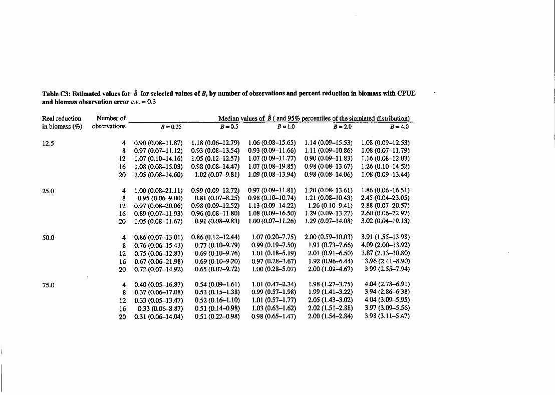
Table C3: Estimated values for k for selected values of B, by number of observations and percent reduction in biomass with CPUE and biomass observation error C.V. = 0.3

Real reduction Number of Median values of ( and 95% percentiles of the simulated distribution) in biomass (%) observations B = 0.25 B = 0.5 B = 1.0 B = 2.0 B = 4.0

APP.ENDIX D: ESTIMATED B PARAMETER (AND 95% CONFIDENCE BOUNDS) FOR NEW ZEALAND SURVEY AND MODEL INDICES, AND NON-NEW ZEALAND SURVEY INDICES

Red gumard: OUR 7

SEW: h n l y Platform

Red gumard: OUR 2

Hoki' Cook Sbait

Red gumard: OUR 3 (b)

Stargazer. STA 5

John dory: J W 1E @)

SEW: Campbell Rise

Hoki: Chatham Rise

Smoothoreo:SS03A

John dory: J W 1E (d)

stargazer: STA 7

Stargazer: STA 2 @)

ORH: NE Chatham Rke @)

Rie: SP07

Stargazer: STA 2 (a)

John dory J W 1 W

Red gumard: OUR 1 W (a)

John dory: J W 2E

ORH: Puysegur

scampi: SCI 1

Ling: Lin 5&6

ORH: NE Chatham R i (a)

Hake: HAK 4

Red gurnard: OUR 1 E (b)

John dory: JOO 1 E (a)

Red gumard: OUR 1W (b)

Ling: UN 3&4

Hold: SubAntarctic (a)

ORH: m a s t coast

Hob West Coast

John dory: J W 2W

Red gumard: GUR 1 E (a)

John dory: JDO 1 E (c)

scam* SCl2

Hdd: Sub-Antarctic @)

Red gurnard: OUR 3 (a)

I I I I 1

0.01 0.1 1 10 100

B (log scale)

Figure Dl: Estimated B parameter (and 95% confidence bounds) for New Zealand survey indices.

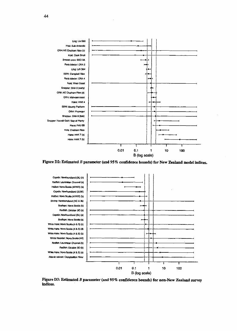
Lins tin 5.36

HW. SubAntarctic

OR& NE Chamam R i e (b)

Hdd: Cook Strait

SmJolhoreo:SS03A

Roc* lobster: CRA 5

Ling UN 384

SBW: Can@xll Rise

Rak lobster: CRA 4

Hold: West Coast

Snapper: SNA 8 (m ORH: NE Chamam R i e (a)

O W Mideast coast

Hake:HAK4

SBW: Bounty Platform

ORK Puysegur

SnapDer: SNA 8 (late)

Snapper: Hauraki Gulf I Bay d Plenty

Paua: PAU 58

Hoki Chatham Aise

Hake: W 7 ( a )

Hake: HAK 7 (b)

0.01 0.1 1 10 100

B (log scale)

Figure D2: Estimated B parameter (and 95% confidence bounds) for New Zealand model indices.

Capelin: Newfoundland (3L) @)

Redfrsh: Laurenlian Channel (a)

Halibut Nova Scotia (4VWX) (a)

W:Nawforardland(21310

Halibut Nova Sc& (4VWX) (b)

Shrirrp:~NewfowMland&ay

Scallops: NovaScolia(b)

R€fnish: Divisian 30 (a)

Wuc Newfwndland (34 (a)

Scalbps: Nova Scolia (a)

White Hake: Nova Scotia (4 B 5) (c)

White Hake: Nwa Scotia (4 & 5) (d)

W h i i H a Nova Sco(ia (4 & 5) (b)

Wmter Aoonder: Nova Smtia (4X)

Redfkh: Laurentian Channel (b)

Redfrrh: War 30 (b)

White Hake: Nova Sco(ia (4 & 5) (a)

AUanntic salmon: -Itan River

0.01 0.1 1 10 100

B (log scale)

F i e D3: Estimated B parameter (and 95 % confidence bounds) for non-New Zealand survey indices.