isse – an interactive source separation editor, part iinjb/research/isse-ii.pdf · non-negative...
TRANSCRIPT

ISSE – An Interactive Source Separation Editor, Part II!
1
Nicholas J. Bryan!Stanford University!
Overview!
§ Introduction!§ Background!§ Approach!§ Algorithm!§ Evaluation!§ Conclusion!
2

Motivation!
§ Real world sounds are mixtures of many individual sounds.!
3
+
Drums Vocals Guitar Bass

Applications I!
§ Denoising!
§ Audio post-production and remastering!
§ Spatial audio and upmixing!
§ Music Information Retrieval!
4

Applications!
§ Music remixing and content creation.!
§ Human-computer interaction perspective.!
§ How does a end-user perform source separation?!
5

Live Demonstration + Sound Examples!
6
Vocal extraction remixes Piano, coughing, denoising
Live demo

Note!
§ Machine learning algorithm that adapts to user annotations.!§ Not copying the pixel data underneath the annotations.!
§ A local annotation can have a global effect.!

Overview!
§ Motivation!§ Background!§ Approach!§ Algorithm!§ Evaluation!§ Conclusion!
8

Overview of Techniques !
Microphone arrays!
Adaptive signal processing!
Independent component analysis!
Computational auditory scene analysis!
Sinusoidal modeling!
Classical denoising and speech enhancement!
Spectral processing!
Time-frequency selection!

Non-Negative Matrix Factorization (NMF) and Related Probabilistic Latent Variable Models (PLVM)!
§ Machine learning, data-driven, basis decomposition, dictionary.!§ Model each sound source within a mixture.!§ Linear combination of prototypical frequency spectra.!§ Well suited to our motivation.!§ Monophonic and/or stereophonic recordings.!§ One of the most promising separation methods of the past decade.!
§ NMF [Lee & Seung, 1999, 2001; Smaragdis & Brown 2003] !
§ PLVM [Raj & Smaragdis 2005, Smaragdis et al., 2006]!
10

Block Diagram!
11
§ Transform signal via the short-time Fourier transform (STFT).!§ Compute a NMF/PLVM.!§ Filter mixture sound.!§ Inverse STFT.!
STFT...
ISTFT
ISTFT
ISTFT
FILTERNMF/PLVM
|X̂1|
|X̂2|
|X̂Ns |
x̂2
x̂1
x̂Ns
x
\X
|X|

The STFT and NMF!
§ The basis vectors capture prototypical frequency content.!§ The weights capture the gains of the basis vectors.!
12

Non-Negative Matrix Factorization!
§ A matrix factorization where everything is non-negative.!§ - original non-negative data!§ - matrix of basis vectors, dictionary elements !§ - matrix activations, weights, or gains!§ (typically)!
13
V 2 RF⇥T+
W 2 RF⇥K+
H 2 RK⇥T+
K < F < T

Optimization Formulation!
§ Minimize the divergence between V and WH.!
!§ At best, find a local optima (not convex).!
14
argmin
W,HD(V |WH)
subject toW � 0,H � 0
DEUC(V |WH) =X
f
X
t
(Vft � [WH]ft)2
DKL(V |WH) =
X
f
X
t
(Vft logVft
[WH]ft� Vft + [WH]ft)
DIS(V |WH) =
X
f
X
t
⇣ Vft
[WH]ft� log
Vft
[WH]ft� 1
⌘
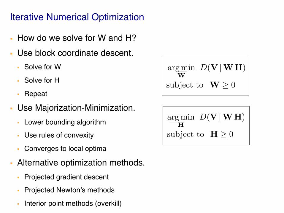
Iterative Numerical Optimization!
§ How do we solve for W and H?!§ Use block coordinate descent.!
§ Solve for W!
§ Solve for H!
§ Repeat!
§ Use Majorization-Minimization.!§ Lower bounding algorithm !
§ Use rules of convexity !
§ Converges to local optima!
§ Alternative optimization methods.!§ Projected gradient descent!
§ Projected Newton’s methods!
§ Interior point methods (overkill)! 15
argmin
HD(V |WH)
subject to H � 0
argmin
WD(V |WH)
subject to W � 0

NMF Parameter Estimation via MM!
§ Initialize to positive random.!§ Repeat until convergence.!
16
H H�WT( V
WH )
WT 1
W W�( VWH )HT
1HT
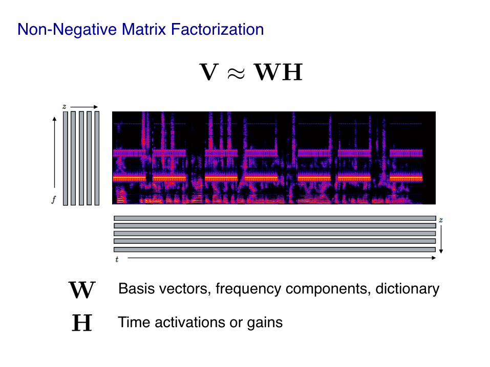
Non-Negative Matrix Factorization!
Basis vectors, frequency components, dictionary!
Time activations or gains!
V ⇡ WH
W
H

Probabilistic Latent Variable Model (PLVM)!• Probabilistic latent component analysis (PLCA).
Basis vectors, frequency components, dictionary!
Time activations or gains! Latent component weights
V ⇡ p(f, t) =Pzp(z)p(f |z)p(t|z)
p(z)
p(f |z)
p(t|z)
p(t|z)
p(z)
p(f |z)

Generative Model!
19
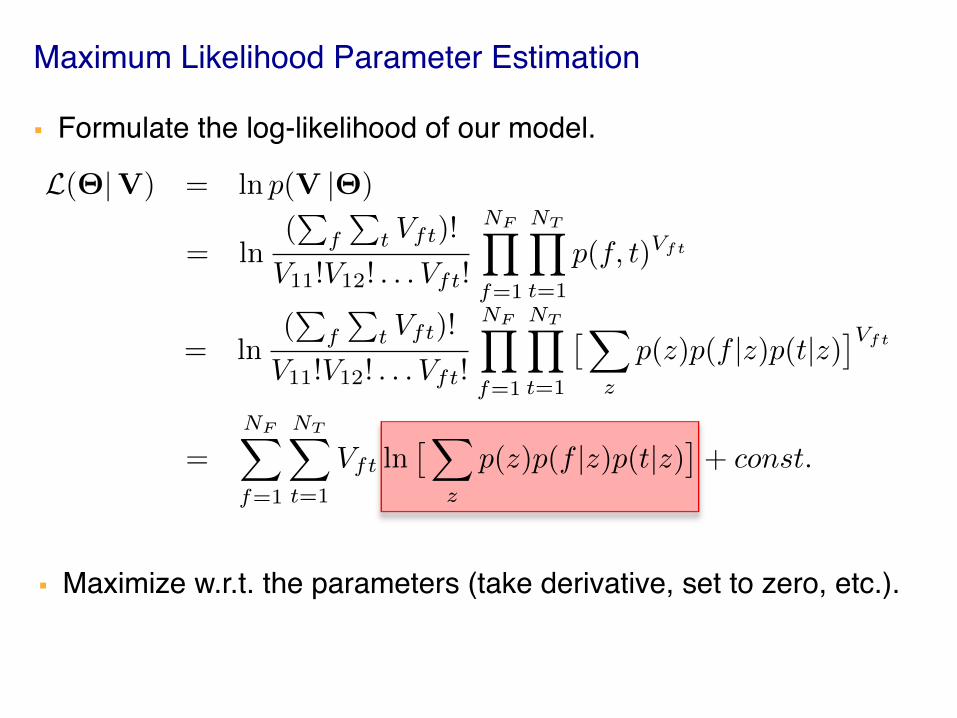
Maximum Likelihood Parameter Estimation!
§ Formulate the log-likelihood of our model.!
20
L(⇥|V) = ln p(V |⇥)
= ln(P
f
Pt Vft)!
V11!V12! . . . Vft!
NFY
f=1
NTY
t=1
p(f, t)Vft
= ln(P
f
Pt Vft)!
V11!V12! . . . Vft!
NFY
f=1
NTY
t=1
⇥X
z
p(z)p(f |z)p(t|z)⇤Vft
=NFX
f=1
NTX
t=1
Vft ln⇥X
z
p(z)p(f |z)p(t|z)⇤+ const.
§ Maximize w.r.t. the parameters (take derivative, set to zero, etc.).!
L(⇥|V) = ln p(V |⇥)
= ln(P
f
Pt Vft)!
V11!V12! . . . Vft!
NFY
f=1
NTY
t=1
p(f, t)Vft
= ln(P
f
Pt Vft)!
V11!V12! . . . Vft!
NFY
f=1
NTY
t=1
⇥X
z
p(z)p(f |z)p(t|z)⇤Vft
=NFX
f=1
NTX
t=1
Vft ln⇥X
z
p(z)p(f |z)p(t|z)⇤+ const.
L(⇥|V) = ln p(V |⇥)
= ln(P
f
Pt Vft)!
V11!V12! . . . Vft!
NFY
f=1
NTY
t=1
p(f, t)Vft
= ln(P
f
Pt Vft)!
V11!V12! . . . Vft!
NFY
f=1
NTY
t=1
⇥X
z
p(z)p(f |z)p(t|z)⇤Vft
=NFX
f=1
NTX
t=1
Vft ln⇥X
z
p(z)p(f |z)p(t|z)⇤+ const.
L(⇥|V) = ln p(V |⇥)
= ln(P
f
Pt Vft)!
V11!V12! . . . Vft!
NFY
f=1
NTY
t=1
p(f, t)Vft
= ln(P
f
Pt Vft)!
V11!V12! . . . Vft!
NFY
f=1
NTY
t=1
⇥X
z
p(z)p(f |z)p(t|z)⇤Vft
=NFX
f=1
NTX
t=1
Vft ln⇥X
z
p(z)p(f |z)p(t|z)⇤+ const.

Expectation Maximization Parameter Estimation I!
§ Formulate the log-likelihood of our model .!§ Form an auxiliary function that lower bounds the log-likelihood.!
21
L(⇥|V)
F(q,⇥) =X
Z
q(Z) ln
⇢p(X,Z |⇥)
q(Z)
�KL(q||p) = KL(q(Z) || p(Z |X,⇥))
= �X
Z
q(Z) ln
⇢p(Z |X,⇥)
q(Z)
�
L(⇥|X) = ln p(X |⇥)
= F(q,⇥) + KL(q||p)� F(q,⇥)
L(⇥|X) = ln p(X |⇥)
= F(q,⇥) + KL(q||p)� F(q,⇥)
L(⇥|X) = ln p(X |⇥)
= F(q,⇥) + KL(q||p)� F(q,⇥)

Expectation Maximization Parameter Estimation II!
§ Iteratively maximize lower bound in two steps (coordinate ascent).!§ E Step: ! ! !
§ M Step:!
!§ Converges to local optima.!
p(Z |X,⇥)
Compute posterior
P (z|f, t)
Update model params
P (f |z)
P (z)
P (t|z)
qn+1= argmax
qF(q,⇥n
)
= argmin
qKL(q||p)
⇥n+1= argmax
⇥F(qn+1,⇥)
Compute the posterior

PLCA Parameter Estimation via EM!
§ Initialize to random probabilities. !§ Repeat until convergence.!
§ E step !
!
§ M step!
P (z|f, t) = P (z)P (f |z)P (t|z)Pz P (z)P (f |z)P (t|z)
P (z) =P
f
Pt VftP (z|f,t)P
z
Pf
Pt VftP (z|f,t)
P (f |z) =P
t VftP (z|f,t)Pf
Pt VftP (z|f,t)
P (t|z) =P
f VftP (z|f,t)Pf
Pt VftP (z|f,t)

Relationship between NMF and PLCA!
§ Equivalent up until init., normalization, reordering of updates.!§ PLCA update equations in matrix notation vs. KL-NMF.!
H H�WT( V
WH )
WT 1
W W�( VWH )HT
1HT
Z V
WH
W W � ZHT
1HT
H H � (WT Z)
PLCA update equations KL-NMF update equations

Modeling and Separating Mixtures!
§ Model each source within a mixture independently.!§ Given a mixture, fix frequency distributions and estimate weights.!
§ Three general classes of techniques [Smaragdis 2007]:!§ Supervised separation!
§ Semi-supervised separation!
§ Unsupervised separation!
§ Use NMF/PLVM output to filter mixture.!
25

Supervised Separation!

Supervised Separation!

Filtering I!
§ Convert source reconstruction into time-varying linear filter.!
!
§ Filter mixture in time-frequency domain.!
§ Inverse STFT with mixture phase .!
§ Overlap-add (OLA) processing to filter mixture [Smith 2011].!
Fs =Ws Hs
WH=
Pz2Zs
p(z)p(f |z)p(t|z)P
z2Z p(z)p(f |z)p(t|z)
|X̂s| = Fs � |X |
\X

Filtering II!
§ Sharp discontinuities in the filter frequency response.!
§ Time-aliasing and other unwanted audible artifacts.!
§ Convert filters to a alias-free form via optimal filter design [Smith 2011].!
§ Incorporate STFT consistency constraints [Le Roux 2013].!
29

Semi-Supervised Separation!

Unsupervised Separation!
§ Without training data….difficult!!

General Problems!
§ Overall a very difficult, ill-posed problem.!
§ Requires isolated training data.!
§ No auditory or perceptual models of hearing.!
§ Cannot correct for poor results (even if obvious).!
32

Overview!
§ Motivation!§ Background!§ Approach!§ Algorithm!§ Evaluation!§ Conclusion!
33
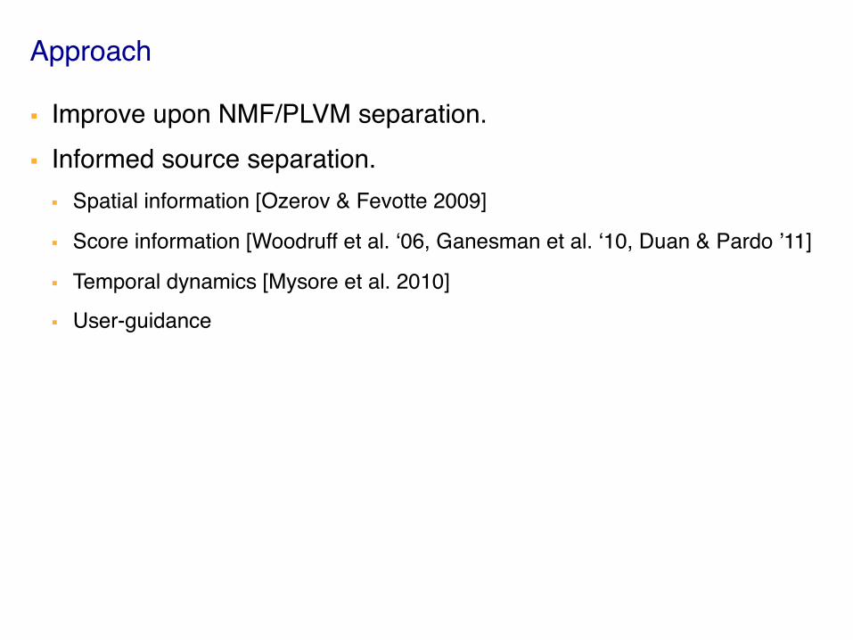
Approach!
§ Improve upon NMF/PLVM separation.!§ Informed source separation.!
§ Spatial information [Ozerov & Fevotte 2009]!
§ Score information [Woodruff et al. ‘06, Ganesman et al. ‘10, Duan & Pardo ’11]!
§ Temporal dynamics [Mysore et al. 2010]!
§ User-guidance!
34

User-Guided Source Separation!
§ Examples: !§ Singing/humming [Smaragdis 2009, Smaragdis and Mysore 2009]!
§ Binary time region annotations [Ozerov et al. 2011, 2012]!
§ Fundamental frequency annotations [Durrieu and Thiran 2012]!
§ Binary time-frequency region annotations [Lefèvre et al. 2012]!
§ Typically no user-feedback, refinement, and/or iteration.!
35

Interactive Source Separation!
§ Extension of user-guided separation.!
§ Subtle, but significant difference.!
§ Two-way communication between user and algorithm.!
§ Emphasize on user-feedback, refinement, and iteration.!
§ Re-compute each interaction.!
§ Requires speed.!
36

Interaction Analogy!
§ Photoshop “layers”!
!!
!
§ 3D Sculpting!
§ User-feedback is key! !
!
37
…
… …

A Layers-Sculpting-Like Interaction for Audio!
38
Speech + Cell Phone!
Speech!
Cell Phone!
looping playback

Interactive Machine Learning!
§ Machine learning (ML) and human-computer interaction (HCI).!§ User-perspective of ML (train and test).!§ We can elicit more information than a class label!!§ Found great success across several domains including:!
§ [Fails & Olsen 2003]!
§ [Fogarty et al. 2008]!
§ [Cohn et al. 2008]!
§ [Settles 2011]!
§ [Fiebrink 2011]!
39
User Correction!
Learning Algorithm!
Unlabeled!Data!
Feedback to User!

Overview!
§ Motivation!§ Background!§ Approach!§ Algorithm!§ Evaluation!§ Conclusion!
40

p(f |z)
p(t|z)
p(z)
Probabilistic Model!
41
V ⇡ P (f, t) =PzP (z)P (f |z)P (t|z)

p(f |z)
p(t|z)
p(z)
Probabilistic Model w/Painting Constraints!
§ Color à source!
§ Opacity à strength!
42
⇤1
⇤2
V ⇡ P (f, t) =PzP̃ (z)P̃ (f |z)P̃ (t|z)

Supervised, Semi-Supervised, & Unsupervised Learning !
§ Supervised!
§ Semi-Supervised!
!§ Unsupervised!

Constraints!
§ Constraints typical encoded as:!§ Prior probabilities on model parameters (e.g. Dirichlet priors)!
§ Direct observations!
§ Does not (reasonably) allow time-frequency constraints!§ Posterior regularization [Graça et al., 2007, Ganchev et al., 2010]!
§ Complementary method that allows time-frequency constraints!
§ Iterative optimization procedure for each E step!
§ Well suited for our problem!
!
44
P (f |z) P (z)P (t|z)
P (z|f, t)

Expectation Maximization!
45
E Step:
M Step:
qn+1= argmax
qF(q,⇥n
)
= argmin
qKL(q||p)
⇥n+1= argmax
⇥F(qn+1,⇥)
L(⇥|X) = ln p(X |⇥)
= F(q,⇥) + KL(q||p)� F(q,⇥)

qn+1= argmax
q2QF(q,⇥n
)
= argmin
q2QKL(q||p)
Expectation Maximization w/Posterior Constraints I!
46
E Step:
M Step: ⇥n+1
= argmax
⇥F(qn+1,⇥)
L(⇥|X) = ln p(X |⇥)
= F(q,⇥) + KL(q||p)� F(q,⇥)

Linear Grouping Expectation Constraints!
47
• For each time-frequency point, solve!
⇤1
⇤2
�T = [⇤1ft ⇤1ft ⇤1ft . . .⇤2ft ⇤2ft ⇤2ft ]
argminq2Q
KL( q(z|f, t) || p(z|f, t) )
argmin
q� qT
lnp+qTlnq+qT �
subject to qT 1 = 1, q � 0

Big Picture!
argminq2Q
KL( q(z|f, t) || p(z|f, t) )
argmin
q� qT
lnp+qTlnq+qT �
subject to qT 1 = 1, q � 0
E Step:
M Step: ⇥n+1
= argmax
⇥F(qn+1,⇥)
Compute posterior
8f, t

Fast, Closed-Form Updates!
49
• With simple penalty, both E and M steps are in closed form.!• Reduces to simple, fast multiplicative updates vs. NMF.!• Roughly the same computational cost as without constraints.!
!• In general, constrained inference would require numerical opt.!

Overview!
§ Motivation!§ Background!§ Approach!§ Algorithm!§ Geometric Interpretation!§ Evaluation!§ Conclusion!
50

Evaluation!
51
§ Initial results!§ Signal Separation Evaluation Campaign (SiSEC) 2013!§ User tests!

Evaluation Metrics!
52
• BSS-EVAL metrics [Vincent et al., 2006]!• (SDR) Signal-to-Distortion Ratio à Overall separation quality!
• (SIR) Signal-to-Interference Ratio à Amount of reduction from unwanted source!
• (SAR) Signal-to-Artifact Ratio à Amount of artifacts introduced by algorithm!
• Baselines!• Ideal, oracle algorithm (soft mask)!
• No user-annotation!
• Past high-performing algorithms!

Initial Results!
• Supervised, semi-supervised, & unsupervised separation comparison!!
!
!
!
!
• Outperformed prior SiSEC 2011 vocals state-of-the-art [Durrieu 2012]!
Example Ideal Supervised Semi-Supervised Unsupervised
Cell 30.7 29.2 / 27.6 28.4 / 06.5 28.8 / -0.6
Drum 14.8 09.7 / 08.5 07.7 / 03.9 10.0 / 00.2
Cough 15.8 14.0 / 12.5 12.0 / 10.5 13.8 / -2.1
Piano 26.1 26.0 / 21.6 14.9 / 08.4 23.1 / 01.1
Siren 27.8 23.8 / 18.9 21.0 / 19.9 24.2 / -4.2
Table 1: SDR (dB) with and without interaction vs. ideal results.
Table 2: SDR (dB) results for the four SiSEC rock/pop songs.
Example Ideal Baseline Lef
´
evre Durrieu Proposed
S1 13.2 -0.8 7.0 9.0 9.2
S2 13.4 0.2 5.0 7.8 11.1
S3 11.5 -0.2 3.8 6.4 7.8
S4 12.5 1.4 5.0 5.9 7.9
Table 1: SDR (dB) with and without interaction vs. ideal results.

Model Selection!
§ How many basis vectors?!§ Set it to a large number (50)!
54
0 20 40 60 80 100 120 140 160 180 200−5
0
5
10
15
20
25
30SDR vs. Basis Vectors
Basis Vectors Per Source (Nz/Ns)
SDR
(dB)
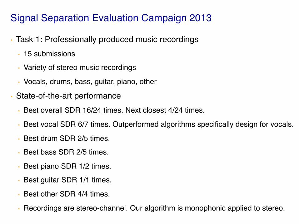
Signal Separation Evaluation Campaign 2013!
• Task 1: Professionally produced music recordings!• 15 submissions!
• Variety of stereo music recordings!
• Vocals, drums, bass, guitar, piano, other!
• State-of-the-art performance!• Best overall SDR 16/24 times. Next closest 4/24 times.!
• Best vocal SDR 6/7 times. Outperformed algorithms specifically design for vocals.!
• Best drum SDR 2/5 times.!
• Best bass SDR 2/5 times. !
• Best piano SDR 1/2 times.!
• Best guitar SDR 1/1 times.!
• Best other SDR 4/4 times.!
• Recordings are stereo-channel. Our algorithm is monophonic applied to stereo.!55

Novice User Evaluation!
§ How well a novice can perform separation?!§ 10 inexperienced users!§ 1 hour long study!
§ Introduction and explanation!§ 5 separation tasks, 10 minutes each, increasing difficulty!§ Exit survey!
§ Measure separation quality per example per user!§ Compare against expert user!§ Tasks:!
§ Cell phone + speech!§ Siren + speech!§ Drums + bass!§ Orchestra + cough!§ Vocals + guitar!
56

Novice User Results I!
§ In some cases, novices outperformed the expert!!
§ Most cases, the expert was best. !
57
1 2 3 4 5−35
−30
−25
−20
−15
−10
−5
0
5
1
234
5
678910
1
2
34
5
6
7
8
9
10
12
3
4
5
6
78
9
10
1
2
3
4
5
67
8
9
10
1
23456
7
8
910
SDR vs. Task
Task
Nor
mal
ized
SD
R (d
B)
Student Version of MATLAB

Novice User Results II!
§ The more difficult the task, the more unsatisfying!
58
1 2 3 4 5
1
2
3
4
5
1
2
3
4
5
6
789
10
1
2
3
45
67
8
910
1
2
3
4
5
6
7
8910 1
2
3
4
5
6
7
8
9
10 1
23
4
56
78
910Satis
fact
ion
Task
Satisfaction Rating vs. Task
Student Version of MATLAB
1 2 3 4 5
1
2
3
4
5
1
2
3
456
78
910
12
3
456
7
8910
12
34
5678
9
10
1
2
3
45
6
7
8
9
10 1
2
3
4
5
6
78
9
10
Diff
icul
ty
Task
Difficulty Rating vs. Task
Student Version of MATLAB
Overview!
§ Motivation!§ Background!§ Approach!§ Algorithm!§ Evaluation!§ Conclusion!
59

Interactive Approach: Benefits!
§ Reduces manual effort. !§ Improves automatic approaches (correct for poor results).!§ No training data needed!!§ Indirectly incorporate a perceptual model.!

Interactive Approach: Problems!
§ Requires a user + learning curve!!§ No guarantee of high-quality results.!§ Overall computation time can be slow.!§ ALL machine learning algorithms require a user.!
§ Who: engineer, scientist, end-user, audio engineer!
§ What: class labeled data, feature labels, other!
§ Where: research laboratory, recording studio, other!
§ When: train and testing occur separately or simultaneously!
§ Why: applications can be different or the same!
!
61
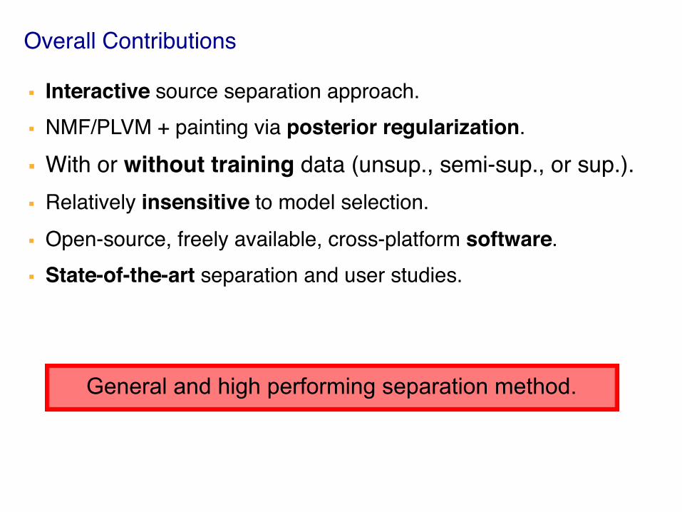
Overall Contributions!
§ Interactive source separation approach.!§ NMF/PLVM + painting via posterior regularization.!
§ With or without training data (unsup., semi-sup., or sup.).!§ Relatively insensitive to model selection.!§ Open-source, freely available, cross-platform software.!§ State-of-the-art separation and user studies.!!
62
General and high performing separation method.

Publications!
1. N. J. Bryan, G. J. Mysore. “Interactive User-Feedback for Sound Source Separation.” ACM Int. Conf. on Intelligent User-Interfaces, Workshop on Interactive Machine Learning, 2013.!
2. N. J. Bryan, G. J. Mysore. “An Efficient Posterior Regularized Latent Variable Model for Interactive Sound Source Separation.” Int. Conf. on Machine Learning, 2013.!
3. N. J. Bryan, G. J. Mysore. “Interactive Refinement of Supervised and Semi-Supervised Sound Source.” Int. Conf. on Acoustics, Speech, and Signal Processing, 2013.!
4. N. J. Bryan, G. J. Mysore. “Signal Separation Evaluation Campaign (SiSEC) Submission.” http://sisec.wiki.irisa.fr, 2013.!
5. N. J. Bryan, G. J. Mysore, G. Wang. “Source Separation of Polyphonic Music With Interactive User-feedback on a Piano Roll Display.” Int. Society of Music Inf. Retrieval, 2013.!
6. (submitted) N. J. Bryan, G. J. Mysore, G. Wang. “ISSE: An Interactive Source Separation Editor.” Conf. on Human Factors in Computing Systems, 2014.!
63

Software + Code!
§ http://isse.sourceforge.net!
§ Application + Code!§ OSX, Windows, Linux!
§ C++ and Matlab code!
§ User forum, wiki, user manual, audio and video demonstrations!
§ Application Web Statistics !§ 2000+ downloads (60+ countries, 36% Japan, 28% USA)!
§ 3600+ Soundcloud listens (13+ hours of audio listened)!
§ 4000+ Youtube views (10+ days of video watched)!
§ 8000+ webpage visits (14.5+ days of viewing)!
64

Thank you!!
65
Work advised by:!Gautham J. Mysore &!
Prof. Ge Wang!

References I!
§ [Lee & Seung, 1999] D. D. Lee and H. S. Seung, “Learning the parts of objects by non-negative matrix factorization.” Nature, 1999.!
§ [Lee & Seung, 2001] D. D. Lee and H. S. Seung, “Algorithms for non-negative matrix factorization.” NIPS, 2001.!
§ [Smaragdis & Brown 2003] P. Smaragdis and J. C. Brown, “Non-negative matrix factorization for polyphonic music transcription.” WASPAA, 2003.!
§ [Fails & Olsen 2003] J. A. Fails and D. R. Olsen, “Interactive machine learning.” IUI, 2003.!
§ [Raj & Smaragdis 2005] B. Raj and P. Smaragdis, “Latent variable decomposition of spectrograms for single channel speaker separation.” WASPAA, 2005.!
§ [Smaragdis et al., 2006] P. Smaragdis, B. Raj, and M. Shashanka, “A probabilistic latent variable model for acoustic modeling.” NIPS Workshop on Acoustic Processing, 2006.!
§ [Woodruff et al. 2006] J. F. Woodruff, B. Pardo, and R. B. Dannenberg, “Remixing stereo music with score-informed source separation.” ISMIR, 2006.!
66

References II!
§ [Vincent et al., 2006] E. Vincent, R. Gribonal, C. Fevotte, “Performance measurement in blind audio source separation.” IEEE TASLP, 2006.!
§ [Graça et al., 2007] J. Graça, K. Ganchev, B. Taskar, “Expectation maximization and posterior constraints.” NIPS, 2007.!
§ [Smaragdis 2007] P. Smaragdis, B. Raj, M. Shashanka, “Supervised and semi-supervised separation of sounds from single-channel mixtures.” ICASS, 2007.!
§ [Fogarty 2008] J. Fogarty, D. Tan, A. Kapoor, S. Winder, “Cueflik: interactive concept learning in image search.” CHI, 2008.!
§ [Cohn et al. 2008] D. Cohn, R. Caruana, A. McCallum, “Semi-supervised clustering with user feedback.” Constrained Clustering: Advances in Algorithms, Theory, and Applications, 2008.!
§ [Smaragdis 2009] P. Smaragdis, “User guided audio selection from complex sound mixtures.” UIST, 2009. !
§ [Smaragdis and Mysore 2009] P. Smaragdis and G. J. Mysore, “Separation by humming: User guided sound extraction from monophonic mixtures.” WASPAA, 2009.!
67

References III!
§ [Ozerov & Fevotte 2009] A. Ozerov and C. Fevotte, “Multichannel nonnegative matrix factorization in convolutive mixtures.” ICASSP, 2009.!
§ [Ganchev et al., 2010] K. Ganchev, J. Graça, J. Gillenwater, B. Taskar, “Posterior regularization for structured latent variable models.” JMLR, 2010.!
§ [Ganesman et al. 2010] J. Ganseman, G. J. Mysore, J. S. Abel, P. Scheunders, “Source separation by source synthesis.” ICMC, 2010.!
§ [Mysore et al. 2010] G. J. Mysore, P. Smaragdis, B. Raj, “Non-negative hidden Markov modeling of audio with application to source separation” LVA/ICA, 2010.!
§ [Settles 2011] “Closing the loop: Fast, interactive semi-supervised annotation with queries on features and instances.” EMNLP, 2011.!
§ [Fiebrink 2011] “Real-time human interaction with supervised learning algorithms for music composition and performance.” PhD Dissertation, Princeton University, 2011.!
§ [Smith 2011] J. Smith, Spectral Audio Signal Processing. W3K Pub., 2011.!
68

References IV!
§ [Duan & Pardo 2011] Z. Duan, B. Pardo, “Soundprism: An online system for score-informed source separation of music audio.” IEEE Journal on Selected Topics in Signal Processing, 2011.!
§ [Ozerov et al. 2011] A. Ozerov, C. Fevotte, R. Blouet, and J.-L. Durrieu, “Multichannel nonnegative tensor factorization with structured constraints for user-guided audio source separation.” ICASSP, 2011.!
§ [Durrieu & Thiran, 2012] J.-L. Durrieu J.-P. Thiran, “Musical audio source separation based on user-selected f0 track.” LVA/ICA, 2012.!
§ [Lefèvre et al. 2012] A. Lefèvre, F. Bach, and C. Fevotte, “Semi-supervised NMF with time-frequency annotations for single-channel source separation.” ISMIR, 2012.!
§ [Ozerov et al. 2012] A. Ozerov, N. Q. Duong, L. Chevallier, “Weighted nonnegative tensor factorization with application to user-guided audio source separation.” Tech Report, 2012.!
§ [Le Roux 2013] J. Le Roux, E. Vincent, “Consistent Weiner Filtering for Audio Source Separation.” IEEE Signal Processing Letters, 2013.!
69

Extra!
70

Alternative (Common) View of EM!
§ View I – expected log-likelihood, then maximize!
§ E step - calculate the expected value of the log-likelihood function!
§ M step – find the parameters that maximize the expected log-likelihood !
!
§ Equivalent, but less general viewpoint!
71
Q(⇥|⇥t) = EZ |X,⇥t [L(⇥;X,Z)]
⇥t+1= argmax
⇥Q(⇥|⇥t
)

Geometric Interpretation!
72
Low (1,0,0)
Mid (0,1,0)
High (0,0,1)Low (1,0,0)
Mid (0,1,0)
High (0,0,1)Low (1,0,0)
Mid (0,1,0)
High (0,0,1)Low (1,0,0)
Mid (0,1,0)
High (0,0,1)Low (1,0,0)
Mid (0,1,0)
High (0,0,1)Low (1,0,0)
Mid (0,1,0)
High (0,0,1)
Source 1Source 2Source 1 Convex HullSource 2 Convex HullMixture Convex HullSource 1 Basis VectorsSource 2 Basis Vectors

Simplex w/Supervised Separation!
73
Low (1,0,0)
Mid (0,1,0)
High (0,0,1)Low (1,0,0)
Mid (0,1,0)
High (0,0,1)Low (1,0,0)
Mid (0,1,0)
High (0,0,1)Low (1,0,0)
Mid (0,1,0)
High (0,0,1)Low (1,0,0)
Mid (0,1,0)
High (0,0,1)Low (1,0,0)
Mid (0,1,0)
High (0,0,1)Low (1,0,0)
Mid (0,1,0)
High (0,0,1)Low (1,0,0)
Mid (0,1,0)
High (0,0,1) Low (1,0,0)
Mid (0,1,0)
High (0,0,1)Low (1,0,0)
Mid (0,1,0)
High (0,0,1)Low (1,0,0)
Mid (0,1,0)
High (0,0,1)Low (1,0,0)
Mid (0,1,0)
High (0,0,1)Low (1,0,0)
Mid (0,1,0)
High (0,0,1)Low (1,0,0)
Mid (0,1,0)
High (0,0,1)Low (1,0,0)
Mid (0,1,0)
High (0,0,1)Low (1,0,0)
Mid (0,1,0)
High (0,0,1)
Source 1Source 2MixtureMixture EstimateSource 1 EstimateSource 2 EstimateSource 1 Convex HullSource 2 Convex HullMixture Convex HullSource 1 Basis VectorsSource 2 Basis Vectors

Simplex w/Semi-Supervised Separation!
74
Low (1,0,0)
Mid (0,1,0)
High (0,0,1)Low (1,0,0)
Mid (0,1,0)
High (0,0,1)Low (1,0,0)
Mid (0,1,0)
High (0,0,1)Low (1,0,0)
Mid (0,1,0)
High (0,0,1)Low (1,0,0)
Mid (0,1,0)
High (0,0,1)Low (1,0,0)
Mid (0,1,0)
High (0,0,1) Low (1,0,0)
Mid (0,1,0)
High (0,0,1)Low (1,0,0)
Mid (0,1,0)
High (0,0,1)Low (1,0,0)
Mid (0,1,0)
High (0,0,1)Low (1,0,0)
Mid (0,1,0)
High (0,0,1)Low (1,0,0)
Mid (0,1,0)
High (0,0,1)Low (1,0,0)
Mid (0,1,0)
High (0,0,1)
Source 1Source 2MixtureSource 1 Convex HullSource 2 Convex HullMixture Convex HullSource 1 Basis VectorsSource 2 Basis Vectors
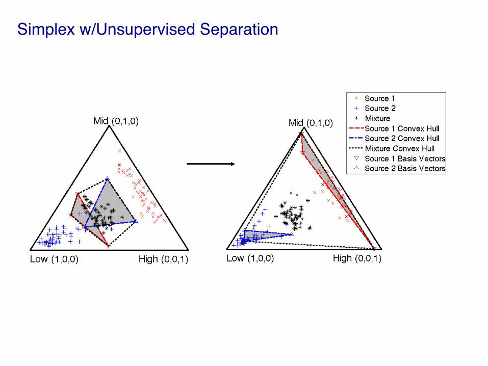
Simplex w/Unsupervised Separation!
75