1

I S S D

Programme interactif de calcul des structures

Interactive Software for Structural Design

Interactief programma voor de berekening van constructies

USER’S GUIDE

- Version September 2007 – ©

Pierre Latteur / Struct&Soft www.issd.be

Av. Fontaine des Fièvres 14, 1495 Villers-la-Ville, Belgium TVA : BE.653.52.173 Trade register 89465

Establishment certificate n°BAS/1999/811/BFR

2

All our thanks to Blaise Rebora, professor at the Polytechnic School of Lausanne, for his contribution to this software.

3

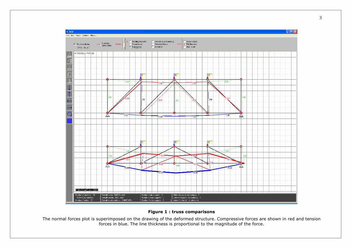
Figure 1 : truss comparisons

The normal forces plot is superimposed on the drawing of the deformed structure. Compressive forces are shown in red and tension forces in blue. The line thickness is proportional to the magnitude of the force.

4

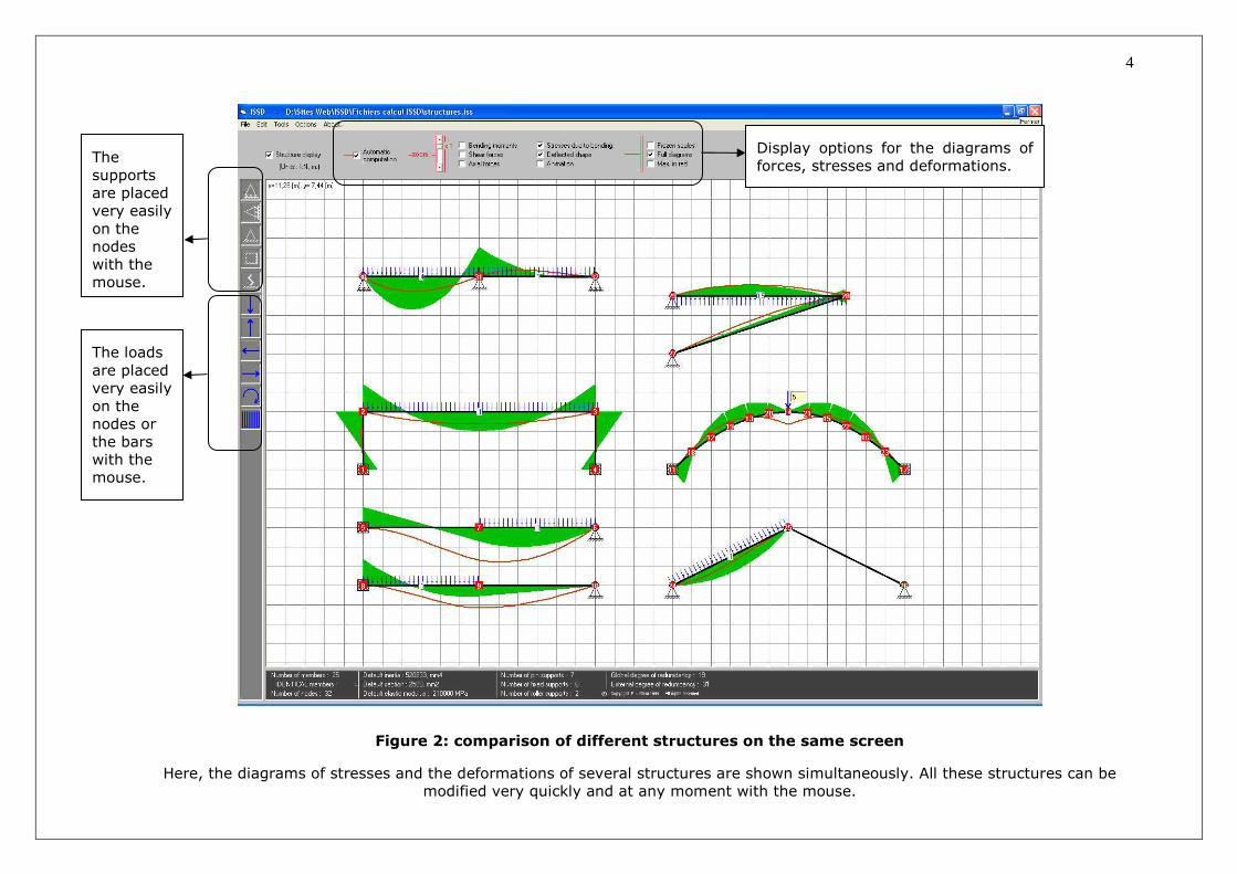
Figure 2: comparison of different structures on the same screen

Here, the diagrams of stresses and the deformations of several structures are shown simultaneously. All these structures can be modified very quickly and at any moment with the mouse.

Display options for the diagrams of forces, stresses and deformations.

The loads are placed very easily on the nodes or the bars with the mouse.

The supports are placed very easily on the nodes with the mouse.

5

Figure 3: the menus “NODE” and “BAR”

These menus appear with a “right click” on a node or a bar. They give all the information related to the selected element

(forces, maximum stresses, geometry, material, support reactions, etc).

« BAR » MENU

« NODE » MENU

1. INTRODUCTION

The majority of commercial software, distributed by the suppliers on the European market, can perform very complex calculations ranging from dynamic analysis, calculation of instabilities to time responses.

However, control of this software requires regular use, several dozens of hours of familiarization and reading of tiresome instructions.

One observation becomes crystal clear: the software which will be used in the decades to come should be able to carry out complex calculations, but should especially be simple and very intuitive to use.

It is rather disconcerting that, from one software to another, the number of operations (e. g. click, double click, confirmation or introduction of certain data, etc) necessary in order to obtain a result is sensibly different. This difference proves that the software developers devote more resources to improve the calculation capacities of their software than to optimize their ergonomics.

The majority of the engineers or architects however frequently need a quick answer (in terms of forces, stresses or displacements) for relatively simple problems, in sketch stage, conceptual phase or budget evaluations: Especially in these circumstances, they need simple, user-friendly and fast 2D software and not the particularly complete set of calculations from traditional software.

These observations led to the idea of conceiving software based primarily on simplicity, ergonomics and the speed of the provided results, while allowing the analysis of complex 2D structures.

Considered as a very powerful didactic work tool for the calculation of structures and material strength, the “career” of ISSD started at European universities or colleges. It was then supplemented to fulfill the requirements of the engineering and design offices (profile catalogues, second order calculation, P-deltas, catalogue of structures, beams on elastic foundation, etc) while preserving its ease of use. Hence, ISSD software is characterized at the same time by an ease of use, pushed to the extreme, and by an advanced capacity of calculation: it could be seen as the “pocket calculator” of the structural engineer of stability, the architect, the engineer on site, the controller or quantity surveyor. We strongly recommend that you read these instructions before using

the software.

7

2. To draw the structure or to change its geometry 2.1. Definition of the working grid, the default material and section type: After having selected New in the File menu, the first step towards the drawing of the structure consists of:

- defining the grid dimensions (by default: 20 m x 10 m with a grid step of 0.5m);

- choosing the default section type (which can be modified afterwards, individually or globally);

- choosing the material type (which can also be modified afterwards, individually or globally).

When the structure is drawn, its nodes will automatically settle on the grid. Their position can be changed to a point which is not defined by the grid points using the menu ‘NODE/move the node’ (see §2.3).

8

2.2. Five ways to draw a bar on the grid The first node of the structure (which will receive index 1) can be placed on a grid by a simple click (left). Another click, elsewhere on the sheet, will determine the position of the node n°2, and the bar which connects them :

There are several ways to draw bars on the work sheet, always by clicking (left) at the place where one wants to place the nodes:

• From an existing node (n°2) to a point of the grid. A new node is then automatically created (here, node n°3):

• From an unspecified point of the grid (new node n°4) to an existing node (node n°2).

• Between two existing nodes. A new bar is automatically created (between nodes 1 and 4) but no new node.

9

• Creation of a new independent bar between two unspecified points on the work sheet. Two new nodes are automatically created (nodes n°5 and 6). In this way, one can draw completely independent structures on the same screen.

There is a last very simple and rapid way to create bars on the screen; very useful when one wants to draw a frame. Therefore, it is necessary to have ticked the option Menu/Options/Automatic panel generation in advance:

By a click (left) on a bar and dragging and dropping with the mouse, on creates automatically, when the mouse button is released, two new bars with a common node: 2.3. To modify the geometry of the structure: Whether the structure is completely drawn or not, whether it is calculated or not, it is possible to modify very quickly and at any moment its geometry, the position of its nodes, their articulated or rigid nature and the sections and materials defined for each bar. The same reasoning goes for the loads and the supports (see §4)

New panel with 2 bars, automatically created from bar n° 4-5

10

• To move a node WITH THE MOUSE on a point defined by the grid: it is enough to place the cursor of the mouse on the node, to click (left) while maintaining the mouse button inserted, and to release the node at the selected place. This action will automatically settle the point on the nearest point of the grid.

•••• To move a node on an point which is NOT defined by the grid:

Position the mouse cursor on the node and click right. The node menu related to this node is displayed. Click on Move the node and define in the appearing window the new co-ordinates (x, y) of your node. Important remark: the node n°1 always corresponds to the co-ordinates (0,0).

•••• To pin or fix a node:

In the same node menu, you can choose the option Pin the node (the node is then represented by a ball) or fix the node (the node is then represented by a square)..

Hinge node

Fixed node

11

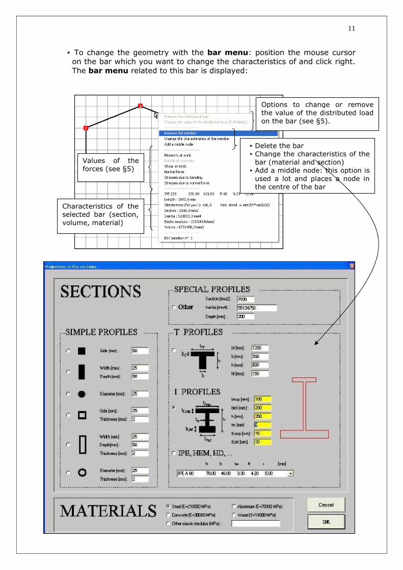
• To change the geometry with the bar menu: position the mouse cursor on the bar which you want to change the characteristics of and click right. The bar menu related to this bar is displayed:

Options to change or remove the value of the distributed load on the bar (see §5).

Values of the forces (see §5)

• Delete the bar • Change the characteristics of the bar (material and section)

• Add a middle node: this option is used a lot and places a node in the centre of the bar

Characteristics of the selected bar (section, volume, material)

12

Note: how to model cables or bars which can only carry axial forces ?

→ It is enough to allot to the section of the bar a very low value of product I.E, which is equivalent to give it a zero bending rigidity. In other words one can give value 1 to both the inertia and the modulus of elasticity. However, the cross sectional surface has to be given exactly:

Example for a suspended bridge :

13

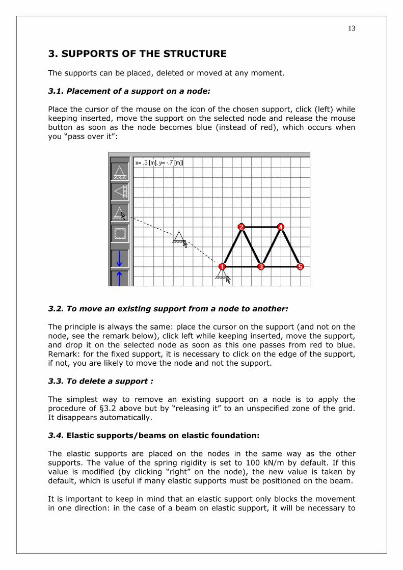
3. SUPPORTS OF THE STRUCTURE The supports can be placed, deleted or moved at any moment. 3.1. Placement of a support on a node: Place the cursor of the mouse on the icon of the chosen support, click (left) while keeping inserted, move the support on the selected node and release the mouse button as soon as the node becomes blue (instead of red), which occurs when you “pass over it”:

3.2. To move an existing support from a node to another: The principle is always the same: place the cursor on the support (and not on the node, see the remark below), click left while keeping inserted, move the support, and drop it on the selected node as soon as this one passes from red to blue. Remark: for the fixed support, it is necessary to click on the edge of the support, if not, you are likely to move the node and not the support. 3.3. To delete a support : The simplest way to remove an existing support on a node is to apply the procedure of §3.2 above but by “releasing it” to an unspecified zone of the grid. It disappears automatically.

3.4. Elastic supports/beams on elastic foundation:

The elastic supports are placed on the nodes in the same way as the other supports. The value of the spring rigidity is set to 100 kN/m by default. If this value is modified (by clicking “right” on the node), the new value is taken by default, which is useful if many elastic supports must be positioned on the beam. It is important to keep in mind that an elastic support only blocks the movement in one direction: in the case of a beam on elastic support, it will be necessary to

14

place an extra roller with horizontal reaction on one of the nodes in order to block the beam in its axial direction. Example: one considers a beam of 10 meters placed on the ground. This ground is modeled by an elastic support at every meter with a value of 147 kN/m. The procedure is as follows:

- providing a grid mesh of 1 m - drawing, with the mouse, 10 pieces of 1 meter each

- placing the first elastic support on node 1 and the stabilizing roller on one of the nodes:

- changing the value of the elastic support to 147 kN/m :

- dropping the 9 other elastic supports, with the default value of 147 kN/m :

- placing the loads and calculating the structure :

15

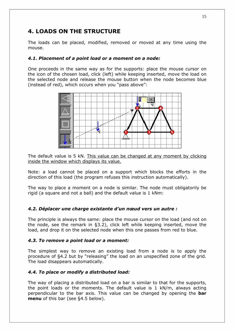
4. LOADS ON THE STRUCTURE The loads can be placed, modified, removed or moved at any time using the mouse. 4.1. Placement of a point load or a moment on a node: One proceeds in the same way as for the supports: place the mouse cursor on the icon of the chosen load, click (left) while keeping inserted, move the load on the selected node and release the mouse button when the node becomes blue (instead of red), which occurs when you “pass above”:

The default value is 5 kN. This value can be changed at any moment by clicking inside the window which displays its value. Note: a load cannot be placed on a support which blocks the efforts in the direction of this load (the program refuses this instruction automatically). The way to place a moment on a node is similar. The node must obligatorily be rigid (a square and not a ball) and the default value is 1 kNm:

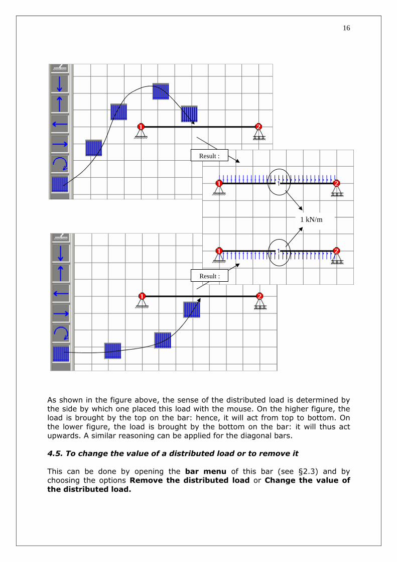
4.2. Déplacer une charge existante d’un nœud vers un autre : The principle is always the same: place the mouse cursor on the load (and not on the node, see the remark in §3.2), click left while keeping inserted, move the load, and drop it on the selected node when this one passes from red to blue. 4.3. To remove a point load or a moment: The simplest way to remove an existing load from a node is to apply the procedure of §4.2 but by “releasing” the load on an unspecified zone of the grid. The load disappears automatically. 4.4. To place or modify a distributed load: The way of placing a distributed load on a bar is similar to that for the supports, the point loads or the moments. The default value is 1 kN/m, always acting perpendicular to the bar axis. This value can be changed by opening the bar menu of this bar (see §4.5 below).

16

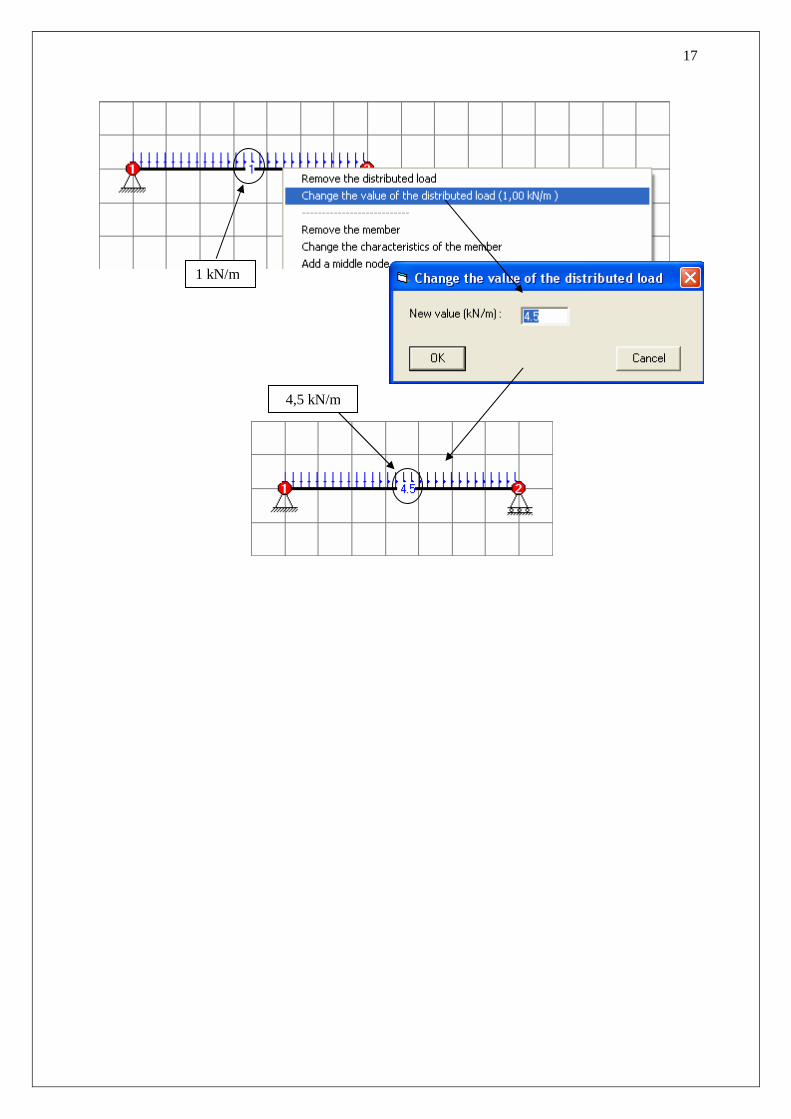
As shown in the figure above, the sense of the distributed load is determined by the side by which one placed this load with the mouse. On the higher figure, the load is brought by the top on the bar: hence, it will act from top to bottom. On the lower figure, the load is brought by the bottom on the bar: it will thus act upwards. A similar reasoning can be applied for the diagonal bars. 4.5. To change the value of a distributed load or to remove it This can be done by opening the bar menu of this bar (see §2.3) and by choosing the options Remove the distributed load or Change the value of

the distributed load.

1 kN/m

Result :

Result :

17

1 kN/m

4,5 kN/m

18

5. DISPLAYING THE DIAGRAMS OF FORCES, STRESSES AND DISPLACEMENTS

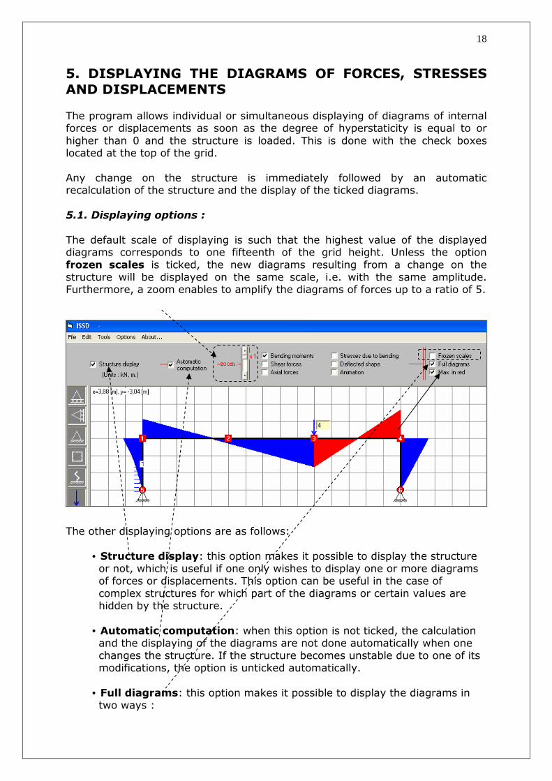
The program allows individual or simultaneous displaying of diagrams of internal forces or displacements as soon as the degree of hyperstaticity is equal to or higher than 0 and the structure is loaded. This is done with the check boxes located at the top of the grid. Any change on the structure is immediately followed by an automatic recalculation of the structure and the display of the ticked diagrams. 5.1. Displaying options : The default scale of displaying is such that the highest value of the displayed diagrams corresponds to one fifteenth of the grid height. Unless the option frozen scales is ticked, the new diagrams resulting from a change on the structure will be displayed on the same scale, i.e. with the same amplitude. Furthermore, a zoom enables to amplify the diagrams of forces up to a ratio of 5.

The other displaying options are as follows:

• Structure display: this option makes it possible to display the structure or not, which is useful if one only wishes to display one or more diagrams of forces or displacements. This option can be useful in the case of complex structures for which part of the diagrams or certain values are hidden by the structure. • Automatic computation: when this option is not ticked, the calculation and the displaying of the diagrams are not done automatically when one changes the structure. If the structure becomes unstable due to one of its modifications, the option is unticked automatically. • Full diagrams: this option makes it possible to display the diagrams in two ways :

19

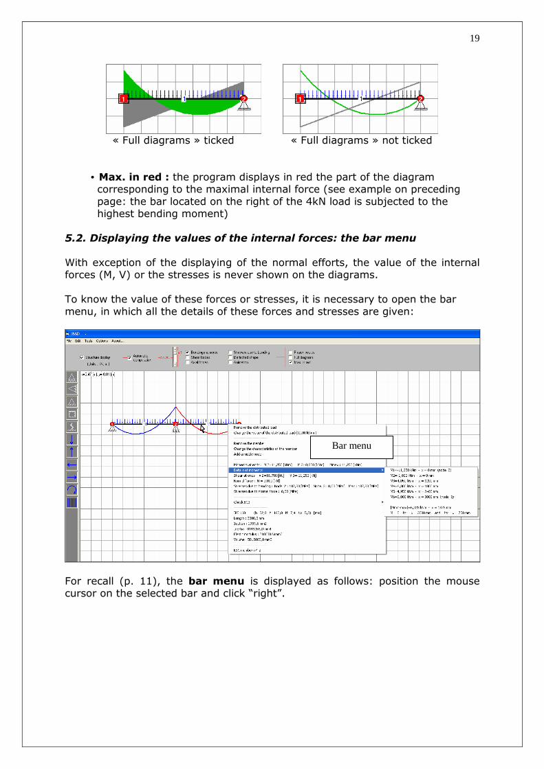
« Full diagrams » ticked « Full diagrams » not ticked

• Max. in red : the program displays in red the part of the diagram corresponding to the maximal internal force (see example on preceding page: the bar located on the right of the 4kN load is subjected to the highest bending moment)

5.2. Displaying the values of the internal forces: the bar menu With exception of the displaying of the normal efforts, the value of the internal forces (M, V) or the stresses is never shown on the diagrams. To know the value of these forces or stresses, it is necessary to open the bar menu, in which all the details of these forces and stresses are given:

For recall (p. 11), the bar menu is displayed as follows: position the mouse cursor on the selected bar and click “right”.

Bar menu

20

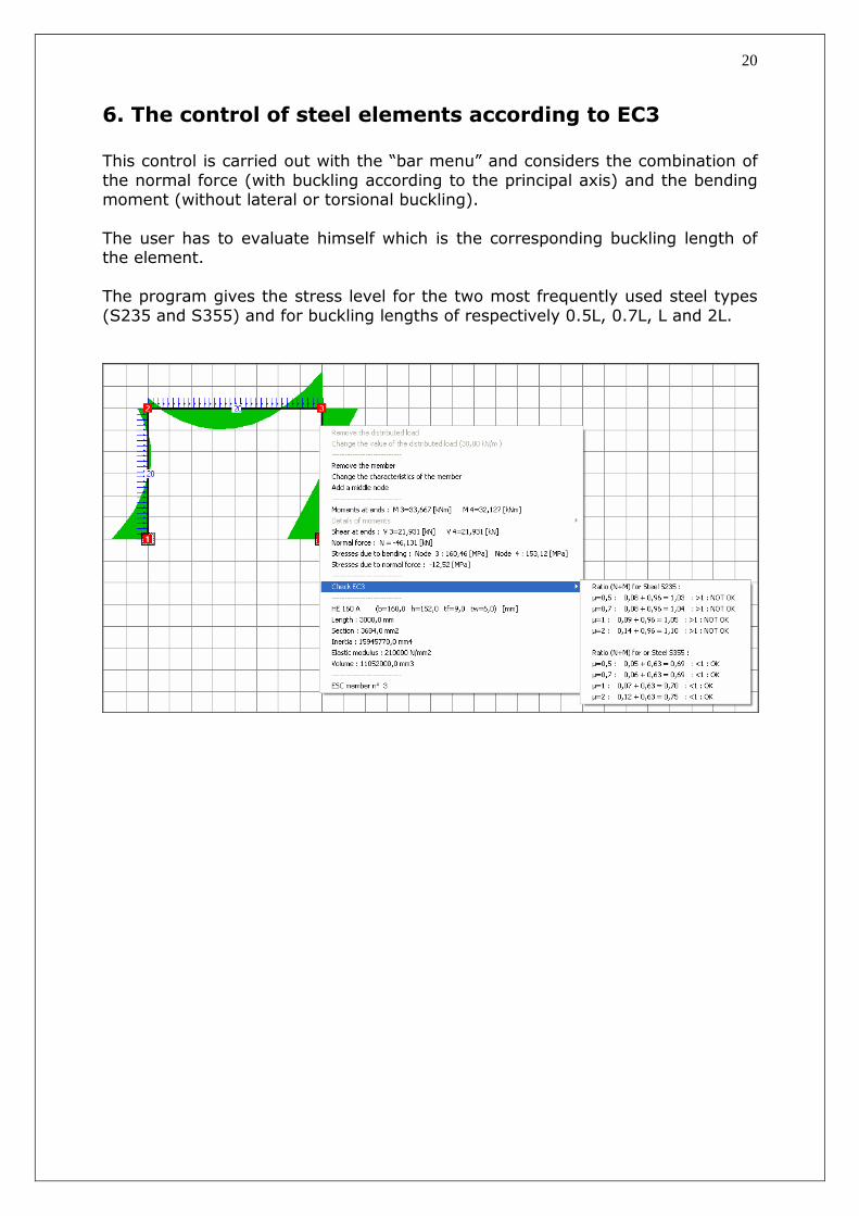
6. The control of steel elements according to EC3 This control is carried out with the “bar menu” and considers the combination of the normal force (with buckling according to the principal axis) and the bending moment (without lateral or torsional buckling). The user has to evaluate himself which is the corresponding buckling length of the element. The program gives the stress level for the two most frequently used steel types (S235 and S355) and for buckling lengths of respectively 0.5L, 0.7L, L and 2L.

21

7. Other possibilities: principal menus

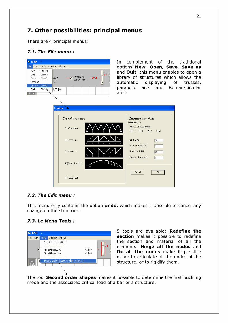
There are 4 principal menus: 7.1. The File menu :

In complement of the traditional options New, Open, Save, Save as and Quit, this menu enables to open a library of structures which allows the automatic displaying of trusses, parabolic arcs and Roman/circular arcs:

7.2. The Edit menu : This menu only contains the option undo, which makes it possible to cancel any change on the structure. 7.3. Le Menu Tools :

5 tools are available: Redefine the section makes it possible to redefine the section and material of all the elements. Hinge all the nodes and fix all the nodes make it possible either to articulate all the nodes of the structure, or to rigidify them.

The tool Second order shapes makes it possible to determine the first buckling mode and the associated critical load of a bar or a structure.

22

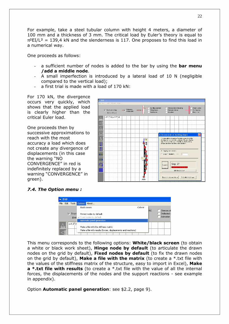
For example, take a steel tubular column with height 4 meters, a diameter of 100 mm and a thickness of 3 mm. The critical load by Euler’s theory is equal to π²EI/L² = 139,4 kN and the slenderness is 117. One proposes to find this load in a numerical way. One proceeds as follows:

- a sufficient number of nodes is added to the bar by using the bar menu /add a middle node.

- A small imperfection is introduced by a lateral load of 10 N (negligible compared to the vertical load);

- a first trial is made with a load of 170 kN: For 170 kN, the divergence occurs very quickly, which shows that the applied load is clearly higher than the critical Euler load. One proceeds then by successive approximations to reach with the most accuracy a load which does not create any divergence of displacements (in this case the warning “NO CONVERGENCE” in red is indefinitely replaced by a warning “CONVERGENCE” in green). 7.4. The Option menu :

This menu corresponds to the following options: White/black screen (to obtain a white or black work sheet), Hinge node by default (to articulate the drawn nodes on the grid by default), Fixed nodes by default (to fix the drawn nodes on the grid by default), Make a file with the matrix (to create a *.txt file with the values of the stiffness matrix of the structure, easy to import in Excel), Make

a *.txt file with results (to create a *.txt file with the value of all the internal forces, the displacements of the nodes and the support reactions - see example in appendix). Option Automatic panel generation: see $2.2, page 9).

23

8. Particular warnings, behaviors and limitations of the software 8.1. Hidden nodes : A node can be moved on the grid, either with the mouse, or with the instruction node menu /move the node. Hence, it may be placed on the axis of a bar without being a physical part of this bar. To avoid this kind of confusion between a node which belongs to a bar (left figure below) and a node which is simply hidden by this bar without belonging to it (right figure below), a warning message is displayed.

Node 5 connects the 4 bars physically Node 5 connects bars 3-5 and 4-5 but

bar 1-2 is independent and not loaded.

8.2. ”Large displacements” : When the loads are very important in comparison with the dimensions of the structure or its sections, the software calculates the forces and shows the diagrams on scale, but it also warns you that the displacements are abnormally large:

24

A1. The file “results” (example) *************** NODE DISPLACEMENTS : ************** *' X [mm] Y [mm] Ang. [rad] Node 1 : 5,648 0,137 0,004 Node 2 : 5,520 0,173 -0,001 Node 3 : 0,000 0,000 0,000 Node 4 : 0,000 0,000 0,000 *************** MEMBER FORCES : ***************' Mi [kNm] Mj [KNm] Ti [kN] Tj [kN] N [kN] Member 1 (i= 1 , j= 2) : -13,436083 34,736632 52,900 34,7366 32 -32,984 Member 2 (i= 1 , j= 3) : 13,436087 -27,467156 -32,984 -27,467 156 -52,900 Member 3 (i= 2 , j= 4) : -34,736640 -31,232290 32,984 -31,232 290 -67,100 *************** VALUES OF THE MOMENTS AT MIDDLE DIS TANCE FOR MEMBERS WITH UNIFORM LOADS : ************ ***' Mi(x=0) [kNm] M(L/5) [KNm] M(2L/5) [KN m] M(3L/5) [KNm] M(4L/5) [KNm] Mj (x=L) [KNm] Mmin [KNm] M=0 for x= [m m] Member 1 (i= 1 , j= 2) : -13.43608 11.10381 21.2437 16.98359 -1.676524 -3 4.73663 21.5438 2360.373 and 284 Member 2 (i= 1 , j= 3) : 13.43609 3.442301 -.1514849 2.654729 11.86094 27 .46716 -.1635995 734.1684 and 915 *************** REACTIONS : ***************' Rhor [kN] Rvert [kN] RAng. [kNm] Node 3 : -47,016 52,900 27,46 7 Node 4 : -32,984 67,100 31,23 2

25

THE LIBRARY :