issc discussion paper series - university … · i introduction in this paper, we investigate how a...
TRANSCRIPT

IISSSSCC DDIISSCCUUSSSSIIOONN PPAAPPEERR SSEERRIIEESS
WAGE POLICY, EMPLOYEE TURNOVER AND PRODUCTIVITY.
Arnaud Chevalier(1)
W. S. Siebert(2) Tarja Viitanen(3)
ISSC WP 2003/08
This paper is produced as part of the Policy Evaluation Programme at ISSC; however the views expressed here do not necessarily reflect those of ISSC. All errors and omissions remain those of the author.

Wage policy, employee turnover and productivity
Arnaud Chevalier♠
W. S. Siebert ♣
Tarja Viitanen♦ This version: 31st May 2003 Key Words: Employee turnover, productivity JEL Classification: J22, J3 Abstract: In this paper, we are interested in the effect of pay incentives on labour turnover and productivity. Particularly we use personnel data from a panel of 400 shops from a UK retail chain. The firm uses perfectly flat hourly wage system with no reward for tenure or individual productivity. This system leads to the phenomenon of negative selection, where only employees with lower outside options remain with the firm. We show that negative selection conflicts with human capital so that the relationship between employee turnover and productivity is U-shaped. If negative selection is as important as human capital accumulation in accounting for the U-shape, then devising a wage policy that will reduce negative selection could increase labour productivity considerably. Acknowledgement: The authors want to thank the anonymous firm for kindly providing data on personnel, and the participants at the “Journées de l’ Association Française d’ Economie”, Lyon 2002, for their comments.
♠ Institute for the Study of Social Change, University College Dublin; Centre for the Economics of Education, London School of Economics; and Institute for the Study of Labor (IZA), Bonn. ♣ University of Birmingham ♦ Institute for the Study of Social Change, University College Dublin; and University of Warwick

I Introduction
In this paper, we investigate how a firm’s pay system affects worker turnover
and thereby labour productivity. Five years of data from approximately 400 shops of a
nationwide retailer are the subject of the analysis. This firm has a very simple pay
system for its shop assistants, with no elements either of seniority pay or
incentive/piece-rate pay. Pay is simply by the hour, distinguishing four regions (with
pay the highest in the London area, and least in rural areas), and a pay increment for
over-18s. Thus for an adult shop assistant, the wage structure of the firm is perfectly
flat1. We present a model showing how this pay system leads to a U-shaped
relationship between productivity and tenure. The upward arm of the U is explained
by the usual human capital reasoning, namely, that productivity increases with tenure.
We argue that the downward arm is explained by negative selection effects, namely,
the more productive workers leaving the firm as they realise they have better outside
options.
Evidence of negative selection has not so far been reported in the literature.
The literature has mostly concentrated on the relationship between pay and tenure
(Barth, 1997, Bingley and Westergaard-Nielsen, 1999 or Farber, 1999 for a survey)
rather than that between productivity and tenure. However, the mechanism we
describe is the mirror of Lazear’s (2000) argument. Lazear estimates that a firm
changing its compensation system from time to piece rates increases its labour
productivity (see also Paarsch and Shearer, 1999). Lazear furthermore shows (2000,
1347) that the productivity gains from piece rates can be divided into two
components: first, average workers increase their effort, and second, there is positive 1 The only way to change one’s wage profile is by promotion to a managerial position. If the probabilities of promotion were large enough, this could be seen as an extreme form of backloaded pay structure, however high promotion rates are not found in the data.
2

selection as more able workers are retained/recruited. In our firm, which offers
straight time rates, we may therefore expect negative selection of workers.
We are not arguing that piece rates are better than time rates. While our results
imply that the firm’s choice of payment system reduces labour productivity, the
opposite could well be true for profitability. Many factors other than labour
productivity affect profitability. Such factors include the cost of an alternative pay
system, and worker responses to the chosen system, as well as the costs of recruiting
and training newcomers (see Brown et al, 2001, 28). Like Lazear (2000, 1359), we are
most interested in workers responses to incentives, and the phenomenon of negative
selection. However, we will make some observations on the profitability issue at the
end.
Our plan is as follows. In the next section, we set out a model linking tenure,
wages and labour productivity. In the third section, we discuss the data available from
the panel of shops. The fourth section presents our estimates of the determinants of
hourly sales per worker (the measure of labour productivity). Here we show the U-
shaped link between labour productivity and tenure. In the final section we draw some
conclusions.
II Model
The model is based on Lazear (2000). In this simple version, we do not assume
any firm-specific human capital. Human capital is measured by a single entity called
“ability”, which can be interpreted as a measure of general human capital. Start by
defining the utility of a worker as a function of his/her wage (W) and effort (e).
3

(1) e) U(W,Utility =
where utility is increasing in wages and decreasing in effort.
The worker’s effort and ability (A) determine the level of output (Q) produced
per pay period.
) (2) ,( AefQ =
where fe, fA > 0. As Lazear notes (2000, 1348), with this specification, for a given Q0
e
A
ff
Ae
−=∂∂ < 0,
meaning that more able workers require less effort to provide Q0. The “cost of effort”
is lower for the more able. More able workers consequently have flatter indifference
curves.
Let us also assume, as is usual when analysing time payment systems, that a
minimum required level of output can be observed by a supervisor, and thus enforced
and determined in the worker’s contract. Hence, the firm rewards the worker with a
flat wage (W0), say, so long as the worker reaches the required output level (Q0). If
the worker does not produce Q0, the contract is terminated. Also, a higher minimum
level of output (Q1) would require more effort and/or ability, and need to be
accompanied by a higher wage (W1). The high minimum output contract will be more
attractive to the high ability group, since their cost of effort is lower.
This model is shown in Figure 1. Firm 1 pays W0 for employees producing
minimum output Q0. The firm employs two types of workers; the less able with
indifference curves such as Ul, and the more able with indifference curves such as Uh.
4

Both types of workers produce the same output Q0 and Firm 1 cannot distinguish
between them. Now assume that a competing firm (Firm 2) offers wages W1 for
workers producing output Q1. Clearly, low ability workers cannot, without reducing
their utility, move to firm 2 and produce Q1. On the other hand, the more able workers
increase their utility to U’h by working in Firm 2.
In order to picture the sorting process, we need to imagine that workers are not
fully aware of their ability when they enter the labour market, and so workers of both
ability types join both firms2. Then, in firm 2, lower ability workers eventually either
realise that they cannot produce output Q1 at their desired level of effort (given wage
W1) and quit, or the supervisors realise this fact, and they are dismissed. On the other
hand, able workers, as they realise their ability, attempt to leave firm 1, applying to
work at firm 2. In firm 1, the average ability of the workforce is reduced, and longer
tenure is a signal for lower ability. Firm 1 experiences negative selection whilst Firm
2 experiences positive selection. With time, the distribution of ability becomes more
homogenous within firm and more heterogenous between firms. This model fits the
stylised worker turnover facts identified by Farber (1999, 2441), namely, that most
new jobs end early and the probability of a job ending declines with tenure (as
employees discover their ability, and move to work for the firm maximising their
utility3).
2 Similar conclusions regarding the sorting of workers may be reached if we assume a matching model where high ability workers work at firm 1 until they receive an offer from firm 2. At each period, more able workers have a propensity hγ , lh γγ > , of exiting firm 1. 3 This last stylised fact is dependent on the frequency of the observations. In the immediate period after the match is created, tenure and separations may be positively related (Farber, 1999). When a job starts, employer and employee have imperfect information relative to the quality of the match. Since destroying the match is costly, the current match has a positive option value (Jovanovitch, 1979). The option value of the match reduces the probability of separation, but as the quality of the match is revealed, the option value diminishes, and the negative relationship between tenure and separation is restored.
5

To apply the model to our population of shops, let us first take the operation of
the selection process in a particular shop. Illustrative numbers are given in Table 1,
keying the figures to actual shop (log) productivity at various levels of worker tenure,
as shown in the last column. If the two ability types were equally represented in the
economy, at the beginning of the first period the shop’s labour productivity would be
the average for both types of workers, that is, 3.98. However, at the end of the period
some matches are terminated, with the more able workers having a higher probability
of separating ( lh γγ > ). Hence, the proportion of less able workers increases through
time and the shop’s average labour productivity tends towards the less able workers’
productivity.
Table 1 presents results assuming a worker’s productivity is a function of his
type (i=high ability, low ability), and tenure in the shop (t):
tiii gxpPtP )( e)( 0 += .
This specification allows productivity to increase with tenure, as in the standard
human capital model, though growth is higher for the high ablity types ( ). We
also assume that the proportion of high ability types declines over time, due to the
negative selection process. As can be seen, during the first 2 years, human capital
gains are then not enough to compensate for the loss of the able types, so that the
shop’s labour productivity declines to 3.92. However, from the third year onwards,
the proportion of able workers declines below one-third of the workforce, reducing
the negative selection effect on shop productivity, and allowing human capital gains
of less able workers to compensate. The selection mechanism added to the human
lh gg >
6

capital effect can thus lead to a U-shaped relationship between a shop’s labour
productivity and its workers’ average tenure.
Figure 2 illustrates the U-shaped relationship. Quadrant II shows the
productivity-tenure link. Here, the segment A’B’ reflects the negative selection of
workers. The steepness of the A’C’ segment is a function of the human capital
accumulation of the workers. Quadrant I shows the productivity-turnover link, which
is the reverse of Quadrant II due to the inverse relationship between tenure and
turnover. Here shops on the AB segment experience negative selection.
Now let us take our population of shops. We imagine this population contains
shops at all stages of the evolution described in Table 1. The shops themselves do not
change over time, but differences in the circumstances of the shops generate the data.
In particular, the outside options of workers in London and large towns are richer than
in rural areas. Hence, there is more labour turnover in London and large towns
(average tenure equals about 1 year), and able workers quickly leave. The negative
selection effect predominates. By contrast, in country shops turnover is lower
(average tenure approaches 3 years). While the able types have left, the remaining
workers have long service and their human capital accumulation compensates. Shops
in intermediate areas have the worst of both worlds, losing the able types, but with too
much turnover among the less able to make up the difference.
7

III The Data
The data comes from a large retailer whose shops are found all over the UK.
Their basis is a register of all employees with an employment spell during the period
1st April 1994 to 1st April 19994. We observe 30,486 individuals and 33,706 spells.5
The analysis is conducted at the shop level, because we do not have measures of
labour productivity at the individual level. The company provided us with information
on annual sales of each shop, as well as some shop characteristics such as location,
type of franchise, and date of latest refurbishment. Using the number of hours
contractually worked6 by employees on the 1st of April of each year, we calculated
sales per hour worked for each shop. This is our measure of labour productivity. As
Table 2 shows, labour productivity has remained relatively stable up to 1998, and then
increased for the last period of observation (coinciding with the introduction of the
National Minimum Wage in April 1999). The distribution of labour productivity
among the shops is shown in Figure 4. At the median, labour productivity is £60, but
the distribution is well dispersed, with a long upper tail. The shops in the upper tail
are from the flagship shops in central London.
We also calculate employee turnover data for each shop. We define turnover as
the ratio of full time equivalent employees joining or quitting a given outlet during the
fiscal year to the number of employees at the end of the fiscal year. Each observation
4 We can observe match as short as one day, hence a more accurate turnover can be calculated than in studies relying on annual data. 5 Unfortunately, employees with multiple spells, due either to change of outlet or time out the company, had their records altered and only information on the last/current spell is available. 6 Contractual hours may not be the same as actual hours worked. However, it has always been company policy to pay for contractual rather than actual hours. In other words, there are no workers simply “on call”, and paid only for hours worked (sonetimes called “zero hours” contracts). Therefore, we expect workers to work at least contractual hours, though they could work more.
8

is weighted by the number of hours worked in a week in order to obtain full time
equivalent turnover. Turnover is calculated for each year and each shop7. Shops
where the total number of working hours was less than 30 (5% of the distribution)
were dropped for that year to reduce measurement error. Also, another 79
shops/observations were dropped as hours worked was missing for more than 15% of
the employees. This leaves us with 520 shops for which we compute average shop
personnel characteristics for age and gender.
Additionally, to help pick up outside options available to employees, we added
information at the county level (66 counties). This set of variables includes the gross
wage of employees in the county, the gross wage of shop assistants and the
unemployment rate. This county level information is calculated from the Quarterly
Labour Force Survey 1995q2 to 1999q4 on a restricted sample of individuals age 16
to 65. This sample is also used to calculate the average unemployment rate in the
county8.
As noted at the beginning, the firm relies on a fixed pay structure, with shops
having no discretionary power. All employees at the shop assistant level are paid at
the same rate whatever their tenure9. Pay varies according to four regions, depending
on the location of the shop (rural, urban, large agglomeration, Central London). In
1999, the adult hourly wage rates for the four locations were respectively: £3.90, 7 For employees with missing hours, we impute their number of hours as the mean of the hours worked in that shop for that specific year. Ten employees who had started on the last day of the year were imputed with the mean over the previous fiscal year. 8 Since the QLFS reports wages only in the first and fifth wave, only individuals in those waves were kept. For each year, we discard the top and bottom 1 percent of the hourly wage distribution, in order to improve the accuracy of the mean wage calculated. The mean hourly wage is then computed for each year and each county. As for the mean gross hourly wage of shop assistants, this calculation is based on a sample of 14,148 shop assistants in the QLFS. 9 The firm discriminates by age, under 18 are paid between 80% and 85% of the adult wage. As for adults, younger workers wage rates are fixed and only dependent on the location of the shop.
9

£4.15, £4.54 and £5.04. These wages are about £1.00 per hour less than the mean
wage for shop assistants in the county (see Table 2).
Given the low relative wage, the firm can be expected to have high labour
turnover. Measuring turnover as the annual staff leaving rate, the figure averages at
about 50% across the shops, though increasing somewhat over the 5 years (see Table
2). In fact, this figure is somewhat lower than the 57% annual staff leaving rate found
for the retail chain in Brown et al (2001, Table 34). Another comparison is to be
found in Cully et al (1999, 133), from the Workplace Employment Relations Survey,
which gives 29% for the annual separation rate (voluntary resignations plus
dismissals) in wholesale and retail. Against these yardsticks, labour turnover in our
shops does not seem particularly high. Nevertheless, we are concerned about the
possible effects of measurement error, so we mark all shops with labour turnover
greater than the 99th percentile. All the shops for which at least one observation is
marked are dropped from the analysis in order to keep a balanced panel of 429 shops
(for 5 years, giving 2145 shop/year points) 10.
The remaining shop level characteristics are given in Table 2. As can be seen
from the top row, retailing is a female dominated occupation with more than 90% of
employees being female. The average employee is in her early thirties, though this
average conceals a wide dispersion, with a large proportion of 16-18 year old
employees. The proportion of workers working less than 5 hours a week, typically to
cover the Saturday rush, has been increasing over the period, nearly tripling from 6%
to 16%. This increase in low-hours work may be the reason why labour turnover has
10 Our results are not sensitive to the trimming of shops for which one observation of turnover is misreported, the results obtained with the resulting unbalanced panel are similar to those presented.
10

increased over the period. The final rows contrast average pay in the company with
that outside, both for workers as a whole, and for shop assistants. As can be seen, the
company’s pay relativity with outside levels for shop assistants has remained very
steady, at about 80% for the 5-year period.
IV Results
In this empirical section, our labour productivity (Q/L) regression model is
specified as follows:
Ln(Q/L)it = αi + βt + γTit + δTit2 + f(Xit, Yit, Zit)
where we log the dependent variable so as to reduce the distortion caused by it long
upper tail (see Figure 3). The αi (i = 1…435) are fixed shop effects, t (= 1…5) are year
effects, and T and T2 are intended to capture the U-shape in labour turnover (T)
explained above11. The αi take account of unobserved shop fixed effects on
productivity, in particular a “desirable” shop location. The year effects are intended to
pick up the business cycle.
Further controls for personnel characteristics are contained in Xit, which
includes gender and age composition, and part-time work composition. Controls for
characteristics of the shop itself are contained in Yit, which includes the shop’s size,
its brand (some shops sell more expensive merchandise than others), the management
area (there are 20 of these, and some regional managers might do better than others),
whether the shop has been recently refurbished, and the shop’s pay (4 pay regions, as
noted). Finally, Zit controls for characteristics of the shop’s local area, namely, the
11 For purposes of the regression, instead of the more usual “leaving rate” (leavers as a percent of the workforce), we use the total turnover rate, that is, the sum of joiners and leavers as a percent of the workforce, which is twice the leaving rate for a stable shop. For shops which are expanding or contracting the total turnover rate is preferable.
11

local average wage, and the unemployment rate. Local conditions will affect shop
sales and thus labour productivity; they will also affect T via their impact on workers’
outside options, as noted above.
Results of the regressions are contained in Table 3. Looking briefly at the
controls, as can be seen, the smaller shops, with an older workforce and a larger
proportion of part-timers (working less than 30 hours a week) appear to be more
productive. The part-timer effect presumably reflects the easier position of staff in
shops with concentrated weekend sales. As might be expected, adverse local
economic conditions (high unemployment and low average wage) reduce labour
productivity.
Now consider the coefficients for turnover. Turnover initially has a negative
effect on productivity, -.069. However, the quadratic term is also significant. For
shops with total turnover greater than 1.19, the relationship becomes positive. A third
of the shops experience a positive relationship between turnover and productivity and
shops with the highest turnover are in fact the most productive. This pattern is
demonstrated in Figure 5. Figure 5 reports the residuals from the fixed effects
equation with the turnover terms excluded. The relationship between the unexplained
productivity and turnover is clearly non-linear. The estimate from a non-parametric
specification indicates a U-shape relationship between turnover and productivity.
Employees quickly gather information on the quality of the match and the more
productive workers exit the firm as they realise their productivity is above the shop
requirement.
12

A random effects specification is also presented in Table 3. As can be seen, the
coefficients between the two models are not very different but a Hausman test rejects
that the differences are not systematic. The random effect model leads to similar
conclusion regarding the relationship between turnover and productivity. Taking the
point estimates at face value, the negative effect of turnover in this specification is
somewhat smaller, -.041, so the proportion of shops on the positive slope is even
higher than in the fixed effect model, reaching 51%.
The random effects specification also allows us to include the effect of time-
invariant variables, in particular the company’s pay structure, as shown by the
Paycode variables. The base category here is the rural paycode, so the figure for
Central London, 0.586, indicates that labour productivity is 58.6% higher in this area.
However, as noted above, the company’s pay rate in the Central London area is only
30% higher than in the rural area (£5.04 compared to £3.90), indicating a degree of
underpayment – consistent with negative selection and the higher turnover observed
for shops in London (30% more than urban shops). Interestingly, the local pay
variable has a significantly negative coefficient in this specification, -0.471. This
negative effect indicates labour productivity is lower in areas with relatively high
local pay rates, implying that the more productive workers leave for better pay in
these areas, which is again consistent with the negative selection.
Column 1 reports the results from a regression were the panel element is not
included. In this cross sectional data, we cannot find a significant relationship
between turnover and productivity. This regression confirms the importance of
controlling for fixed effects in an analysis of shop productivity.
13

As predicted by our theoretical model, the relationship between turnover and
productivity is non linear. The non-linearity is driven by the conflicting forces of a
positive effect of human capital accumulation and the negative effect of workers
selection. We have conjectured that employee selection is driven by the availability
of outside options we further test this assumption by focusing on the determinants of
turnover. The influence of relative pay on worker’s decision to leave is shown in
Figure 6. Here we have formed the residuals from a labour turnover regression
omitting relative pay, and graph these residuals on a relative pay variable. A negative
relationship can be seen. Relative pay therefore has the influence on worker mobility
decisions that we expect12.
Our results have implications for the company’s wage policies, and it is
interesting to speculate a little. The wage policy is endogenous, any change in the
wage policy would move the firm to a different U-shape function. The functions will
become flatter and flatter as the wage structure reduces negative selection, until there
is no negative selection and the strict human capital model is restored. Our back of the
envelope calculations are only based on movement on the current line and can
therefore be seen as under-estimates of the true productivity gains to be made by a
reduction in negative selectivity.
Raising company pay by 10% would reduce turnover by at least this amount
according to Brown et al (2001, 37) – though somewhat less according to our Figure
6. Every 10% decline in turnover increases labour productivity by around 4% once we
are on the beneficial side of the U (segment CA in Panel 1 of Figure 3). To this 4%
12 Similarly, we estimated the effect of local unemployment on mobility, but no relationship was found. The lack of significance of the unemployment may reflect that our proxy does not measure the outside options available to workers of this company, or that it does not capture the local labour market conditions. These results are available from the authors.
14

benefit we can also add 1% due to the benefit of savings on training and recruitment
costs due to lower turnover13. However, the 5% saving is still less than the 10% cost.
At the same time, it must be remembered that the 5% saving is an underestimate. It is
calculated according to the existing U-shape, not to the new, higher shape that would
result if there were reduced negative selection. Inspection of Figure 5 shows how
labour productivity varies by about 40% (log labour productivity varies from about
4.2 to 4.6) across the shops. Some, perhaps half, of this variation will be due to
negative selection (as in Lazear, 2000). Thus, there is plenty of scope to increase
labour productivity, which makes us believe that the 5% benefit is a considerable
underestimate of the 10% wage increase.
Conclusion
In this paper, we have investigated the sensitivity of workers to incentives. In
particular, we have shown using the personnel records from a UK retailer that workers
facing higher relative wage are more likely to terminate their contract. The paper adds
to the literature on the impact of the pay structure on employee’s quality by putting
forward a model in which the relationship between labour turnover and labour
productivity is non-linear.
The model introduces the concept of negative workforce selection. The non-
linearity is driven by the conflicting forces of human capital and negative selectivity
on productivity. Lazear (2000), and Paarsch and Shearer (1999) for example, estimate
that half the productivity gains of moving from an input-based wage to a piece-rate
wage are due to positive workers selection. In our analysis, we highlight the mirror
13 For every 10% reduction in turnover, an amount equal to 1% of the wage bill is saved because training and recruitment costs are avoided (Brown et al, 2001, Table 23).
15

problem of negative selection for a firm paying a flat wage. As their productivity is
not rewarded, the more able employees have a higher propensity of leaving the firm
than the less able. We have argued that the negative employee selection is driven by
the differing availability of outside options among the company’s hundreds of shops.
The company’s flat wage system, without seniority or bonus elements, and only
differentiating between four regions, cannot track the outside options. The result,
therefore, is negative selection which leads to a U-shaped relationship between
tenure/turnover and productivity.
Since the pay structure of the firm is endogenous the analysis has its limit and
does not allow us to calculate the expected productivity gains that would be achieved
if the firm were to increase wages or introduce a performance related pay-structure.
Tentatively, we note that at the current wage, monitoring and production function, a
10% increase in pay would lead to at least a 5% increase in the average productivity.
Our results introduce a new consideration for company wage policy. In the
company we find a 40% systematic variation in labour productivity among the shops.
The U-shaped relationship between labour productivity and labour turnover is deep. If
negative selection is as important as human capital accumulation in accounting for the
U-shape, then devising a wage policy that will reduce negative selection would
increase labour productivity considerably.
16

Reference:
Barth E. (1997) “Firm specific seniority and wages” Journal of Labor Economics, 15, 495-
506
Bingley P. and N. Westergaard-Nielsen (1999) “The effect of firm pay policy on worker
turnover”, CLS, University of Aahrus, mimeo
Brown D., R. Dickens, P. Gregg, S. Machin and A. Manning, 2001. Everything Under a
Fiver, York: Joseph Rowntree Foundation Work and Opportunity Series No. 22.
Cully M., S. Woodland, A. O’Reilly and G. Dix, (1999) Britain At Work, London:
Routledge
Davis S., J. Haltiwanger and S. Schuh (1997) “Job creation and destruction”, MIT press
Farber H. (1999) “Mobility and Stability: The dynamic of job change in labor markets” in
Handbook of Labor Economics, Vol 3B, O. Ashenfelter and D. Card (Eds), North-
Holland
Jovanovic B. (1979) “Firm-specific capital and turnover” Journal of Political Economy, 87,
972-990
Lazear E. (2000) “Performance pay and productivity” American Economic Review, 90,
pp1346-61
Paarsch H. and B. Shearer (1999) “The response of worker effort to piece rates” Journal of
Human Resources, 34, pp 643-667
17

Figure 1: Compensation and effort in a two firms, two types of workers model
Uh1
Uh0
W1
W0
Wage UL0
Q1 Q0 Output/Effort
Figure 2: Relationship between productivity, turnover and tenure
negative selection
negative selection
B’
’
I
C’
1
C
8
B
A
A
Q/L
Tenure
Turnover
Q/L
II

Figure 3: Sales per hour at shop level in 1999 Fr
actio
n
(mean) sal_hr990 100 200 300
0
.05
.1
.15
.2
Figure 4: Turnover and productivity
Lowess smoother, bandwidth = .5
Xb
annual turnover0 2 4 6 8
3
3.5
4
4.5
5
19

Figure 5: Relative pay and turnover
Lowess smoother, bandwidth = .5Xb
relpay.4 .6 .8 1 1.2
0
1
2
20

Table 1: Simulated link between tenure and labour productivity
Workforce proportions: Labour productivity: Shop productivity: Tenure (years)
high ability low ability high ability low ability Simulated Actual Type of
region
0.2 0.49 0.51 6.04 2.02 3.99 3.98
1 0.44 0.56 6.22 2.13 3.93 3.93
┐│││┘
High turnover
region, e.g. London
2 0.39 0.61 6.49 2.27 3.92 3.92
3 0.35 0.65 6.82 2.43 3.97 3.97
┐│││┘
Intermed-iate
4 0.31 0.69 7.23 2.62 4.05 4.08
5 0.27 0.73 7.72 2.82 4.14 4.25
┐│││┘
Low turnover
region, e.g. country town
Note: Proportion high ability workers is given by: a * exp (-b * t). Worker productivity is calculated as in the text (P0+exp (g * t) ) where P0 and g are function of the ability type of the worker. The parameters were set to a= 0.5, b= 0.12, P0h= 5, P0l= 1, gh = 0.20, gl = 0.12. Shop productivity: simulated is the weighted average of high and low ability workers; actual productivity is calculated using the coefficients from Table 3.
21
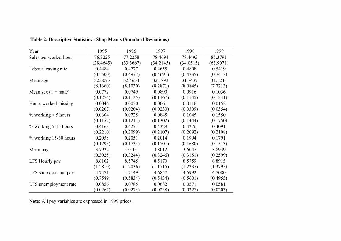
Table 2: Descriptive Statistics - Shop Means (Standard Deviations) Year 1995 1996 1997 1998 1999Sales per worker hour 76.3225
(28.4645) 77.2258
(33.3667) 78.4694
(34.2145) 78.4493
(34.0515) 85.3791
(65.9071) Labour leaving rate 0.4484
(0.5500) 0.4777
(0.4977) 0.4655
(0.4691) 0.4808
(0.4235) 0.5419
(0.7413) Mean age 32.6075
(8.1660) 32.4634 (8.1030)
32.1893 (8.2871)
31.7437 (8.0845)
31.1248 (7.7213)
Mean sex (1 = male) 0.0772 (0.1274)
0.0749 (0.1135)
0.0890 (0.1167)
0.0916 (0.1145)
0.1036 (0.1341)
Hours worked missing 0.0046 (0.0207)
0.0050 (0.0204)
0.0061 (0.0230)
0.0116 (0.0309)
0.0152 (0.0354)
% working < 5 hours 0.0604 (0.1157)
0.0725 (0.1211)
0.0845 (0.1302)
0.1045 (0.1444)
0.1550 (0.1750)
% working 5-15 hours 0.4168 (0.2210)
0.4271 (0.2099)
0.4328 (0.2107)
0.4276 (0.2092)
0.4091 (0.2108)
% working 15-30 hours 0.2058 (0.1793)
0.2051 (0.1734)
0.2014 (0.1701)
0.1994 (0.1680)
0.1791 (0.1513)
Mean pay 3.7922 (0.3025)
4.0101 (0.3244)
3.8012 (0.3246)
3.6047 (0.3151)
3.8939 (0.2599)
LFS Hourly pay 8.6102 (1.2810)
8.5745 (1.2036)
8.5170 (1.1715)
8.5759 (1.2237)
8.8915 (1.3795)
LFS shop assistant pay 4.7471 (0.7589)
4.7149 (0.5834)
4.6857 (0.5434)
4.6992 (0.5601)
4.7080 (0.4955)
LFS unemployment rate 0.0856 (0.0267)
0.0785 (0.0274)
0.0682 (0.0238)
0.0571 (0.0227)
0.0581 (0.0203)
Note: All pay variables are expressed in 1999 prices.

Table 3: Determinants of Log Sales per Worker Hour
(Standard errors in parentheses)
Variable OLS Fixed effect Random Effect Labour turnover -0.007 -0.069 -0.041 (0.031) (0.021) (0.021) Labour turnover-squared 0.011 0.029 0.025 (0.008) (0.005) (0.005) Shop average age 0.001 0.010 0.002 (0.002) (0.002) (0.001) Shop sex distribution 0.132 -0.067 0.071 (0.099) (0.076) (0.072)
% working <5 hours 0.587 0.629 0.409 (0.141) (0.078) (0.068) % working 5-15 hours 0.288 0.456 0.317 (0.062) (0.057) (0.049) % working 15-30 0.036 0.165 0.033
Hours: (base=% working>30 hours)
hours (0.062) (0.070) (0.057) 5-10 employees -0.144 -0.396 -0.239 (0.018) (0.023) (0.020) 10-20 employees -0.174 -0.644 -0.338 (0.024) (0.039) (0.030) > 20 employees -0.230 -0.874 -0.450
Size: (base= size<5)
(0.045) (0.075) (0.059) More expensive brand 0.529 0.458 (0.050) (0.051) Less expensive brand 0.027 -0.036 (0.021) (0.033) other -0.270 -0.304
Brand: (base= mid range price)
(0.038) (0.047) urban 0.111 0.124 (0.026) (0.034) Agglomeration 0.176 0.146 (0.049) (0.058) Central London 0.464 0.586
Paycode area: (base= rural)
(0.133) (0.137) Local unemployment -0.043 -0.420 -0.293 (0.466) (0.661) (0.490) Local ln pay -0.472 -0.042 -0.471 (0.120) (0.244) (0.147) Dummies for regional manager, date of shop refurbishment, location and year
Yes Yes Yes
Constant 5.262 4.032 5.213 (0.279) (0.524) (0.321) Observations 2145 2145 2145 R-squared 0.38 0.27 0.35