isoperimetric inequalities for eigenvalues of the laplacian

Entropy & the Quantum II, Contemporary Mathematics 552, 21–60 (2011)

Isoperimetric Inequalities for Eigenvalues of the Laplacian

Rafael D. Benguria

Abstract. These are extended notes based on the series of four lectures onisoperimetric inequalities for the Laplacian, given by the author at the Arizona

School of Analysis with Applications, in March 2010.

Mais ce n’est pas tout; la Physique ne nous donne passeulement l’occasion de resoudre des problemes;

elle nous aide a en trouver les moyens, et cela de deux manieres.Elle nous fait presentir la solution;elle nous suggere des raisonaments.

Conference of H. Poincare at the ICM, in Zurich, 1897, see [63], p. 340.

Contents

1. Introduction 222. Lecture 1: Can one hear the shape of a drum? 233. Lecture 2: Rearrangements and the Rayleigh–Faber–Krahn Inequality 314. Lecture 3: The Szego–Weinberger and the Payne–Polya–Weinberger

inequalities 405. Lecture 4: Fourth order differential operators 526. Appendix 55References 56

1991 Mathematics Subject Classification. Primary 35P15; Secondary 35J05, 49R50.

Key words and phrases. Eigenvalues of the Laplacian, isoperimetric inequalities.This work has been partially supported by Iniciativa Cientıfica Milenio, ICM (CHILE),

project P07–027-F, and by FONDECYT (Chile) Project 1100679.c© 2011 by the author. This paper may be reproduced, in its entirety, for non-commercial

purposes.

c©0000 (copyright holder)

21

22 RAFAEL D. BENGURIA

1. Introduction

Isoperimetric inequalities have played an important role in mathematics sincethe times of ancient Greece. The first and best known isoperimetric inequality isthe classical isoperimetric inequality

A ≤ L2

4π,

relating the area A enclosed by a planar closed curve of perimeter L. After theintroduction of Calculus in the XVIIth century, many new isoperimetric inequali-ties have been discovered in mathematics and physics (see, e.g., the review articles[16, 57, 59, 64]; see also the essay [13] for a panorama on the subject of Isoperime-try). The eigenvalues of the Laplacian are “geometric objects” in the sense that theydepend on the geometry of the underlying domain, and to some extent (see Lecture1) the knowledge of all the eigenvalues characterizes several aspects of the geometryof the domain. Therefore it is natural to pose the problem of finding isoperimetricinequalities for the eigenvalues of the Laplacian. The first one to consider this pos-sibility was Lord Rayleigh in his monograph The Theory of Sound [65]. In theselectures I will present some of the problems arising in the study of isoperimetricinequalities for the Laplacian, some of the tools needed in their proof and manybibliographic discussions about the subject. I start this review (Lecture 1) with theclassical problem of Mark Kac, Can one hear the shape of a drum?. In the secondLecture I review some basic facts about rearrangements and the Rayleigh–Faber–Krahn inequality. In the third lecture I discuss the Szego–Weinberger inequality,which is an isoperimetric inequality for the first nontrivial Neumann eigenvalue ofthe Laplacian, and the Payne–Polya–Weinberger isoperimetric inequality for thequotient of the first two Dirichlet eigenvalues of the Laplacian, as well as severalrecent extensions. Finally, in the last lecture I review three different isoperimetricproblems for fourth order operators. There are many interesting results that I haveleft out of this review. For different perspectives, selections and emphasis, pleaserefer, for example, to the reviews [2, 3, 4, 12, 44], among many others. The con-tents of this manuscript are based on a series of four lectures given by the author atthe Arizona School of Analysis with Applications, University of Arizona, Tucson,AZ, March 15-19, 2010. Other versions of this course have been given as an inten-sive course for graduate students in the Tunis Science City, Tunisia (May 21–22,2010), in connection with the International Conference on the isoperimetric prob-lem of Queen Dido and its mathematical ramifications, that was held in Carthage,Tunisia, May 24–29, 2010; and, previously, in the IV Escuela de Verano en Analisisy Fısica Matematica at the Unidad Cuernavaca del Instituto de Matematicas de laUniversidad Nacional Autonoma de Mexico, in the summer of 2005 [20]. Prelimi-nary versions of these lectures were also given in the Short Course in IsoperimetricInequalities for Eigenvalues of the Laplacian, given by the author in February of2004 as part of the Thematic Program on Partial Differential Equations held atthe Fields Institute, in Toronto, and also during the course Autovalores del Lapla-ciano y Geometrıa given by the author at the Department of Mathematics of theUniversidad de Pernambuco, in Recife, Brazil, in August 2003.

I would like to thank the organizers of the Arizona School of Analysis withApplications (2010), for their kind invitation, their hospitality and the opportunity

ISOPERIMETRIC INEQUALITIES FOR EIGENVALUES OF THE LAPLACIAN 23

to give these lectures. I also thank the School of Mathematics of the Institute forAdvanced Study, in Princeton, NJ, for their hospitality while I finished preparingthese notes. Finally, I would like to thank the anonymous referee for many usefulcomments and suggestions that helped to improve the manuscript.

2. Lecture 1: Can one hear the shape of a drum?

...but it would baffle the most skillfulmathematician to solve the Inverse Problem,and to find out the shape of a bell by means

of the sounds which is capable of sending out.Sir Arthur Schuster (1882).

In 1965, the Committee on Educational Media of the Mathematical Association ofAmerica produced a film on a mathematical lecture by Mark Kac (1914–1984) withthe title: Can one hear the shape of a drum? One of the purposes of the film wasto inspire undergraduates to follow a career in mathematics. An expanded versionof that lecture was later published [46]. Consider two different smooth, boundeddomains, say Ω1 and Ω2 in the plane. Let 0 < λ1 < λ2 ≤ λ3 ≤ . . . be the sequenceof eigenvalues of the Laplacian on Ω1, with Dirichlet boundary conditions and,correspondingly, 0 < λ′1 < λ′2 ≤ λ′3 ≤ . . . be the sequence of Dirichlet eigenvaluesfor Ω2. Assume that for each n, λn = λ′n (i.e., both domains are isospectral). Then,Mark Kac posed the following question: Are the domains Ω1 and Ω2 congruentin the sense of Euclidean geometry?. A friend of Mark Kac, the mathematicianLipman Bers (1914–1993), paraphrased this question in the famous sentence: Canone hear the shape of a drum?

In 1910, H. A. Lorentz, during the Wolfskehl lecture at the University ofGottingen, reported on his work with Jeans on the characteristic frequencies ofthe electromagnetic field inside a resonant cavity of volume Ω in three dimensions.According to the work of Jeans and Lorentz, the number of eigenvalues of the elec-tromagnetic cavity whose numerical values is below λ (this is a function usuallydenoted by N(λ)) is given asymptotically by

(2.1) N(λ) ≈ |Ω|6π2

λ3/2,

for large values of λ, for many different cavities with simple geometry (e.g., cubes,spheres, cylinders, etc.) Thus, according to the calculations of Jeans and Lorentz,to leading order in λ, the counting function N(λ) seemed to depend only on thevolume of the electromagnetic cavity |Ω|. Apparently David Hilbert (1862–1943),who was attending the lecture, predicted that this conjecture of Lorentz would notbe proved during his lifetime. This time, Hilbert was wrong, since his own student,Hermann Weyl (1885–1955) proved the conjecture less than two years after thelecture by Lorentz.

Remark: There is a nice account of the work of Hermann Weyl on the eigenvalues ofa membrane in his 1948 J. W. Gibbs Lecture to the American Mathematical Society[78].


In N dimensions, (2.1) reads,

(2.2) N(λ) ≈ |Ω|(2π)N

CNλN/2,

where CN = π(N/2)/Γ((N/2) + 1)) denotes the volume of the unit ball in N dimen-sions.

Using Tauberian theorems, one can relate the behavior of the counting functionN(λ) for large values of λ with the behavior of the function

(2.3) ZΩ(t) ≡∞∑n=1

exp−λnt,

for small values of t. The function ZΩ(t) is the trace of the heat kernel for thedomain Ω, i.e., ZΩ(t) = tr exp(∆t). As we mentioned above, λn(Ω) denotes the nDirichlet eigenvalue of the domain Ω.

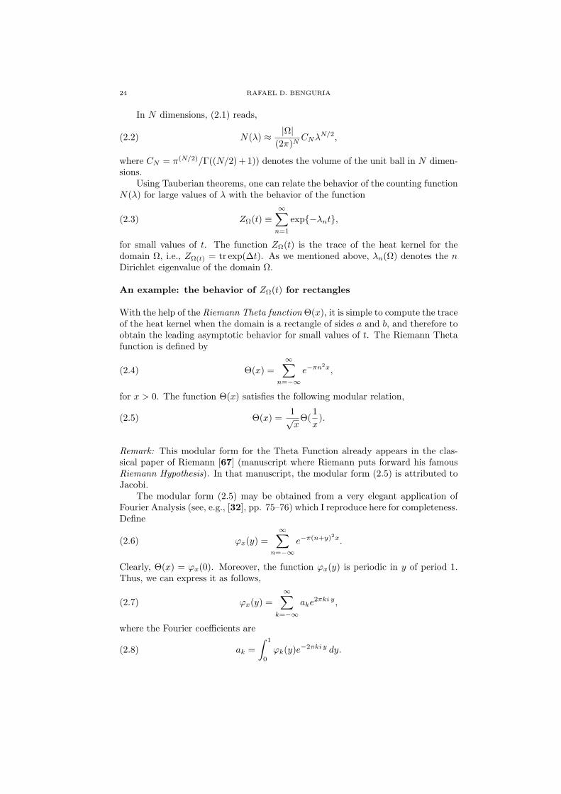
An example: the behavior of ZΩ(t) for rectangles

With the help of the Riemann Theta function Θ(x), it is simple to compute the traceof the heat kernel when the domain is a rectangle of sides a and b, and therefore toobtain the leading asymptotic behavior for small values of t. The Riemann Thetafunction is defined by

(2.4) Θ(x) =∞∑

n=−∞e−πn

2x,

for x > 0. The function Θ(x) satisfies the following modular relation,

(2.5) Θ(x) =1√x

Θ(1x

).

Remark: This modular form for the Theta Function already appears in the clas-sical paper of Riemann [67] (manuscript where Riemann puts forward his famousRiemann Hypothesis). In that manuscript, the modular form (2.5) is attributed toJacobi.

The modular form (2.5) may be obtained from a very elegant application ofFourier Analysis (see, e.g., [32], pp. 75–76) which I reproduce here for completeness.Define

(2.6) ϕx(y) =∞∑

n=−∞e−π(n+y)2x.

Clearly, Θ(x) = ϕx(0). Moreover, the function ϕx(y) is periodic in y of period 1.Thus, we can express it as follows,

(2.7) ϕx(y) =∞∑

k=−∞

ake2πki y,

where the Fourier coefficients are

(2.8) ak =∫ 1

0

ϕk(y)e−2πki y dy.


Replacing the expression (2.6) for ϕx(y) in (2.8), using the fact that e2πki n = 1,we can write,

(2.9) ak =∫ 1

0

∞∑n=−∞

e−π(n+y)2xe−2πik(y+n) dy.

Interchanging the order between the integral and the sum, we get,

(2.10) ak =∞∑

n=−∞

∫ 1

0

(e−π(n+y)2xe−2πik(y+n)

)dy.

In the nth summand we make the change of variables y → u = n + y. Clearly, uruns from n to n+ 1, in the nth summand. Thus, we get,

(2.11) ak =∫ ∞−∞

e−πu2xe−2πik u du.

i.e., ak is the Fourier transform of a Gaussian. Thus, we finally obtain,

(2.12) ak =1√xe−πk

2/x.

Since, Θ(x) = ϕx(0), from (2.7) and (2.12) we finally get,

(2.13) Θ(x) =∞∑

k=−∞

ak =1√x

∞∑k=−∞

e−πk2/x =

1√x

Θ(1x

).

Remarks: i) The method exhibited above is a particular case of the Poisson Sum-mation Formula. See [32], pp. 76–77; ii) It should be clear from (2.4) thatlimx→∞Θ(x) = 1. Hence, from the modular form for Θ(x) we immediately seethat

(2.14) limx→0

√xΘ(x) = 1.

Once we have the modular form for the Riemann Theta function, it is simpleto get the leading asymptotic behavior of the trace of the heat kernel ZΩ(t), forsmall values of t, when the domain Ω is a rectangle. Take Ω to be the rectangle ofsides a and b. Its Dirichlet eigenvalues are given by

(2.15) λn,m = π2

[n2

a2+m2

b2

],

with n,m = 1, 2, . . . . In terms of the Dirichlet eigenvalues, the trace of the heatkernel, ZΩ(t) is given by

(2.16) ZΩ(t) =∞∑

n,m=1

e−λn,mt.

and using (2.15), and the definition of Θ(x), we get,

(2.17) ZΩ(t) =14

[Θ(π t

a2)− 1

] [Θ(π t

b2)− 1

].


Using the asymptotic behavior of the Theta function for small arguments, i.e.,(2.14) above, we have

(2.18) ZΩ(t) ≈ 14

(a√π t− 1)(

b√π t− 1) ≈ 1

4πtab− 1

4√πt

(a+ b) +14

+O(t).

In terms of the area of the rectangle A = ab and its perimeter L = 2(a + b), theexpression ZΩ(t) for the rectangle may be written simply as,

(2.19) ZΩ(t) ≈ 14πt

A− 18√πtL+

14

+O(t).

Remark: Using similar techniques, one can compute the small t behavior of ZΩ(t)for various simple regions of the plane (see, e.g., [50]).

The fact that the leading behavior of ZΩ(t) for t small, for any bounded, smoothdomain Ω in the plane is given by

(2.20) ZΩ(t) ≈ 14πt

A

was proven by Hermann Weyl [77]. Here, A = |Ω| denotes the area of Ω. In fact,what Weyl proved in [77] is the Weyl Asymptotics of the Dirichlet eigenvalues, i.e.,for large n, λn ≈ (4π n)/A. Weyl’s result (2.20) implies that one can hear the areaof the drum.

In 1954, the Swedish mathematician, Ake Pleijel [62] obtained the improvedasymptotic formula,

ZΩ(t) ≈ A

4πt− L

8√πt,

where L is the perimeter of Ω. In other words, one can hear the area and theperimeter of Ω. It follows from Pleijel’s asymptotic result that if all the frequenciesof a drum are equal to those of a circular drum then the drum must itself becircular. This follows from the classical isoperimetric inequality (i.e., L2 ≥ 4πA,with equality if and only if Ω is a circle). In other words, one can hear whether adrum is circular. It turns out that it is enough to hear the first two eigenfrequenciesto determine whether the drum has the circular shape [6]

In 1966, Mark Kac obtained the next term in the asymptotic behavior of ZΩ(t)[46]. For a smooth, bounded, multiply connected domain on the plane (with rholes)

(2.21) ZΩ(t) ≈ A

4πt− L

8√πt

+16

(1− r).

Thus, one can hear the connectivity of a drum. The last term in the above asymp-totic expansion changes for domains with corners (e.g., for a rectangular membrane,using the modular formula for the Theta Function, we obtained 1/4 instead of 1/6).Kac’s formula (2.21) was rigorously justified by McKean and Singer [51]. More-over, for domains having corners they showed that each corner with interior angle γmakes an additional contribution to the constant term in (2.21) of (π2−γ2)/(24πγ).

A sketch of Kac’s analysis for the first term of the asymptotic expansion is asfollows (here we follow [45, 46, 50]). If we imagine some substance concentrated at~ρ = (x0, y0) diffusing through the domain Ω bounded by ∂Ω, where the substance


is absorbed at the boundary, then the concentration PΩ(~p∣∣ ~r ; t) of matter at

~r = (x, y) at time t obeys the diffusion equation∂PΩ

∂t= ∆PΩ

with boundary condition PΩ(~p∣∣ ~r ; t) → 0 as ~r → ~a, ~a ∈ ∂Ω, and initial condition

PΩ(~p∣∣ ~r ; t) → δ(~r − ~p ) as t → 0, where δ(~r − ~p ) is the Dirac delta function. The

concentration PΩ(~p∣∣ ~r ; t) may be expressed in terms of the Dirichlet eigenvalues of

Ω, λn and the corresponding (normalized) eigenfunctions φn as follows,

PΩ(~p∣∣ ~r ; t) =

∞∑n=1

e−λntφn(~p )φn(~r ).

For small t, the diffusion is slow, that is, it will not feel the influence of the boundaryin such a short time. We may expect that

PΩ(~p∣∣ ~r ; t) ≈ P0(~p

∣∣ ~r ; t),

ar t → 0, where ∂P0/∂t = ∆P0, and P0(~p∣∣ ~r ; t) → δ(~r − ~p ) as t → 0. P0 in fact

represents the heat kernel for the whole R2, i.e., no boundaries present. This kernelis explicitly known. In fact,

P0(~p∣∣ ~r; t) =

14πt

exp(−|~r − ~p |2/4t),

where |~r − ~p |2 is just the Euclidean distance between ~p and ~r. Then, as t→ 0+,

PΩ(~p∣∣ ~r ; t) =

∞∑n=1

e−λntφn(~p )φn(~r ) ≈ 14πt

exp(−|~r − ~p |2/4t).

Thus, when set ~p = ~r we get∞∑n=1

e−λntφ2n(~r ) ≈ 1

4πt.

Integrating both sides with respect to ~r, using the fact that φn is normalized, wefinally get,

(2.22)∞∑n=1

e−λn t ≈ |Ω|4πt

,

which is the first term in the expansion (2.21). Further analysis gives the remainingterms (see [46]).

Remark: In 1951, Mark Kac proved the following universal bound on ZΩ(t) indimension d:

(2.23) ZΩ(t) ≤ |Ω|(4πt)d/2

.

This bound is sharp, in the sense that as t→ 0,

(2.24) ZΩ(t) ≈ |Ω|(4πt)d/2

.

Recently, Harrell and Hermi [43] proved the following improvement on (2.24),

(2.25) ZΩ(t) ≈ |Ω|(4πt)d/2

e−Md|Ω|t/I(Ω).


Figure 1. GWW Isospectral Domains D1 and D2

where IΩ = mina∈Rd

∫Ω|x − a|2 dx and Md is a constant depending on dimension.

Moreover, they conjectured the following bound on ZΩ(t), namely,

(2.26) ZΩ(t) ≈ |Ω|(4πt)d/2

e−t/|Ω|2/d

.

Recently, Geisinger and Weidl [38] proved the best bound up to date in this direc-tion,

(2.27) ZΩ(t) ≈ |Ω|(4πt)d/2

e−Mdt/|Ω|2/d

,

where Md = [(d + 2)π/d]Γ(d/2 + 1)−2/dMd (in particular M2 = π/16. In generalMd < 1, thus the Geisinger–Weidl bound (2.27) falls short of the conjecturedexpression of Harrell and Hermi.

2.1. One cannot hear the shape of a drum. In the quoted paper of MarkKac [46] he says that he personally believed that one cannot hear the shape ofa drum. A couple of years before Mark Kac’ article, John Milnor [54], had con-structed two non-congruent sixteen dimensional tori whose Laplace–Beltrami op-erators have exactly the same eigenvalues. In 1985 Toshikazu Sunada [69], thenat Nagoya University in Japan, developed an algebraic framework that provideda new, systematic approach of considering Mark Kac’s question. Using Sunada’stechnique several mathematicians constructed isospectral manifolds (e.g., Gordonand Wilson; Brooks; Buser, etc.). See, e.g., the review article of Robert Brooks(1988) with the situation on isospectrality up to that date in [25] (see also, [27]).Finally, in 1992, Carolyn Gordon, David Webb and Scott Wolpert [40] gave thedefinite negative answer to Mark Kac’s question and constructed two plane domains(henceforth called the GWW domains) with the same Dirichlet eigenvalues.

The most elementary proof of isospectrality of the GWW domains is done using themethod of transplantation. For the method of transplantation see, e.g., [21, 22]. Seealso the expository article [23] by the same author. The method also appears brieflydescribed in the article of Sridhar and Kudrolli [68], cited in the BibliographicalRemarks, iv) at the end of this chapter.


For the interested reader, there is a recent review article [39] that presentsmany different proofs of isospectrality, including transplantation, and paper foldingtechniques).

Theorem 2.1 (C. Gordon, D. Webb, S. Wolpert). The domains D1 and D2 offigures 1 and 2 are isospectral.

Although the proof by transplantation is straightforward to follow, it does notshed light on the rich geometric, analytic and algebraic structure of the probleminitiated by Mark Kac. For the interested reader it is recommendable to read thepapers of Sunada [69] and of Gordon, Webb and Wolpert [40].

In the previous paragraphs we have seen how the answer to the original Kac’s ques-tion is in general negative. However, if we are willing to require some analyticityof the domains, and certain symmetries, we can recover uniqueness of the domainonce we know the spectrum. During the last decade there has been an importantprogress in this direction. In 2000, S. Zelditch, [79] proved that in two dimensions,simply connected domains with the symmetry of an ellipse are completely deter-mined by either their Dirichlet or their Neumann spectrum. More recently [80],proved a much stronger positive result. Consider the class of planar domains withno holes and very smooth boundary and with at least one mirror symmetry. Thenone can recover the shape of the domain given the Dirichlet spectrum.

2.2. Bibliographical Remarks. i) The sentence of Arthur Schuster (1851–1934)quoted at the beginning of this Lecture is cited in Reed and Simon’s book, volume IV[66]. It is taken from the article A. Schuster, The Genesis of Spectra, in Report of thefifty–second meeting of the British Association for the Advancement of Science (held atSouthampton in August 1882). Brit. Assoc. Rept., pp. 120–121, 1883. Arthur Schusterwas a British physicist (he was a leader spectroscopist at the turn of the XIX century).It is interesting to point out that Arthur Schuster found the solution to the Lane–Emdenequation with exponent 5, i.e., to the equation,

−∆u = u5,

in R3, with u > 0 going to zero at infinity. The solution is given by

u =31/4

(1 + |x|2)1/2.

(A. Schuster, On the internal constitution of the Sun, Brit. Assoc. Rept. pp. 427–429,1883). Since the Lane–Emden equation for exponent 5 is the Euler–Lagrange equationfor the minimizer of the Sobolev quotient, this is precisely the function that, modulotranslations and dilations, gives the best Sobolev constant. For a nice autobiographyof Arthur Schuster see A. Schuster, Biographical fragments, Mc Millan & Co., London,(1932).

ii) A very nice short biography of Marc Kac was written by H. P. McKean [Mark Kac inBibliographical Memoirs, National Academy of Science, 59, 214–235 (1990); available onthe web (page by page) at http://www.nap.edu/books/0309041988/html/214.html]. The


reader may want to read his own autobiography: Mark Kac, Enigmas of Chance, Harperand Row, NY, 1985 [reprinted in 1987 in paperback by The University of California Press].For his article in the American Mathematical Monthly, op. cit., Mark Kac obtained the1968 Chauvenet Prize of the Mathematical Association of America.

iii) For a beautiful account of the scientific contributions of Lipman Bers (1993–1914),who coined the famous phrase, Can one hear the shape of a drum?, see the article byCathleen Morawetz and others, Remembering Lipman Bers, Notices of the AMS 42, 8–25(1995).

iv) It is interesting to remark that the values of the first Dirichlet eigenvalues of theGWW domains were obtained experimentally by S. Sridhar and A. Kudrolli, [68]. In thisarticle one can find the details of the physics experiments performed by these authorsusing very thin electromagnetic resonant cavities with the shape of the Gordon–Webb–Wolpert (GWW) domains. This is the first time that the approximate numerical valuesof the first 25 eigenvalues of the two GWW were obtained. The corresponding eigen-functions are also displayed. A quick reference to the transplantation method of PierreBerard is also given in this article, including the transplantation matrix connecting thetwo isospectral domains. The reader may want to check the web page of S. Sridhar’sLab (http://sagar.physics.neu.edu/) for further experiments on resonating cavities, theireigenvalues and eigenfunctions, as well as on experiments on quantum chaos.

v) The numerical computation of the eigenvalues and eigenfunctions of the pair of GWWisospectral domains was obtained by Tobin A. Driscoll, Eigenmodes of isospectral domains,SIAM Review 39, 1–17 (1997).

vi) In their simplified forms, the Gordon–Webb–Wolpert domains (GWW domains) aremade of seven congruent rectangle isosceles triangles. Certainly the GWW domainshave the same area, perimeter and connectivity. The GWW domains are not convex.Hence, one may still ask the question whether one can hear the shape of a convex drum.There are examples of convex isospectral domains in higher dimension (see e.g. C. Gor-don and D. Webb, Isospectral convex domains in Euclidean Spaces, Math. Res. Letts.1, 539–545 (1994), where they construct convex isospectral domains in Rn, n ≥ 4).Remark: For an update of the Sunada Method, and its applications see the articleof Robert Brooks [The Sunada Method, in Tel Aviv Topology Conference “RothenbergFestschrift” 1998, Contemprary Mathematics 231, 25–35 (1999); electronically availableat: http://www.math.technion.ac.il/ rbrooks]

vii) There is a vast literature on Kac’s question, and many review lectures on it. Inparticular, this problem belongs to a very important branch of mathematics: InverseProblems. In that connection, see the lectures of R. Melrose [53]. For a very recentreview on Kac’s question and its many ramifications in physics, see [39].

viii) There is an excellent recent article in the book Mathematical Analysis of Evo-lution, Information, and Complexity, edited by Wolfgang Arendt and Wolfgang P.Schleich, Wiley, 2009, called Weyl’s Law: Spectral Properties of the Laplacian in Math-ematics and Physics, written by Wolfgang Arendt, Robin Nittka, Wolfgang Peter, andFrank Steiner which is free available online, at


http://www.wiley-vch.de/books/sample/3527408304 c01.pdf. That article should be use-ful to the interested reader. It has a thorough discussion about Kac’s problem, Weylasymptotics and the historical beginnings of quantum mechanics

3. Lecture 2: Rearrangements and the Rayleigh–Faber–KrahnInequality

For many problems of functional analysis it is useful to replace some functionby an equimeasurable but more symmetric one. This method, which was first intro-duced by Hardy and Littlewood, is called rearrangement or Schwarz symmetrization[42]. Among several other applications, it plays an important role in the proofsof isoperimetric inequalities like the Rayleigh–Faber–Krahn inequality (see the endof this Lecture), the Szego–Weinberger inequality or the Payne–Polya–Weinbergerinequality (see Lecture 3), and many others. In this lecture we present some basicdefinitions and theorems concerning spherically symmetric rearrangements. For amore general treatment see, e.g., [12, 20, 26, 75] (and also the references in theBibliographical Remarks at the end of this lecture).

3.1. Definition and basic properties. We let Ω be a measurable subset ofRn and write |Ω| for its Lebesgue measure, which may be finite or infinite. If it isfinite we write Ω? for an open ball with the same measure as Ω, otherwise we setΩ? = Rn. We consider a measurable function u : Ω → R and assume either that|Ω| is finite or that u decays at infinity, i.e., |x ∈ Ω : |u(x)| > t| is finite for everyt > 0.

Definition 3.1. The function

µ(t) = |x ∈ Ω : |u(x)| > t|, t ≥ 0

is called distribution function of u.

From this definition it is straightforward to check that µ(t) is a decreasing (non–increasing), right–continuous function on R+ with µ(0) = |sprt u| and sprtµ =[0, ess sup |u|).

Definition 3.2.

• The decreasing rearrangement u] : R+ → R+ of u is the distributionfunction of µ.

• The symmetric decreasing rearrangement u? : Ω? → R+ of u is defined byu?(x) = u](Cn|x|n), where Cn = πn/2[Γ(n/2 + 1)]−1 is the measure of then-dimensional unit ball.

Because µ is a decreasing function, Definition 3.2 implies that u] is an essentiallyinverse function of µ. The names for u] and u? are justified by the following twolemmas:

Lemma 3.3.

(a) The function u] is decreasing, u](0) = esssup |u| and sprtu] = [0, |sprtu|)(b) u](s) = min t ≥ 0 : µ(t) ≤ s(c) u](s) =

∫∞0χ[0,µ(t))(s) dt

(d) |s ≥ 0 : u](s) > t| = |x ∈ Ω : |u(x)| > t| for all t ≥ 0.(e) s ≥ 0 : u](s) > t = [0, µ(t)) for all t ≥ 0.


Proof. Part (a) is a direct consequence of the definition of u], keeping in mindthe general properties of distribution functions stated above. The representationformula in part (b) follows from

u](s) = |w ≥ 0 : µ(w) > s| = supw ≥ 0 : µ(w) > s = minw ≥ 0 : µ(w) ≤ s,

where we have used the definition of u] in the first step and then the monotonicityand right-continuity of µ. Part (c) is a consequence of the ‘layer-cake formula’, seeTheorem 6.1 in the appendix. To prove part (d) we need to show that

(3.1) s ≥ 0 : u](s) > t = [0, µ(t)).

Indeed, if s is an element of the left hand side of (3.1), then by Lemma 3.3, part(b), we have

minw ≥ 0 : µ(w) ≤ s > t.

But this means that µ(t) > s, i.e., s ∈ [0, µ(t)). On the other hand, if s is anelement of the right hand side of (3.1), then s < µ(t) which implies again by part(b) that

u](s) = minw ≥ 0 : µ(w) ≤ s ≥ minw ≥ 0 : µ(w) < µ(t) > t,

i.e., s is also an element of the left hand side. Finally, part (e) is a direct consequencefrom part (d).

It is straightforward to transfer the statements of Lemma 3.3 to the symmetricdecreasing rearrangement:

Lemma 3.4.

(a) The function u? is spherically symmetric and radially decreasing.(b) The measure of the level set x ∈ Ω? : u?(x) > t is the same as the

measure of x ∈ Ω : |u(x)| > t for any t ≥ 0.

From Lemma 3.3 (c) and Lemma 3.4 (b) we see that the three functions u,u] and u? have the same distribution function and therefore they are said to beequimeasurable. Quite analogous to the decreasing rearrangements one can alsodefine increasing ones:

Definition 3.5.

• If the measure of Ω is finite, we call u](s) = u](|Ω| − s) the increasingrearrangement of u.• The symmetric increasing rearrangement u? : Ω? → R+ of u is defined byu?(x) = u](Cn|x|n)

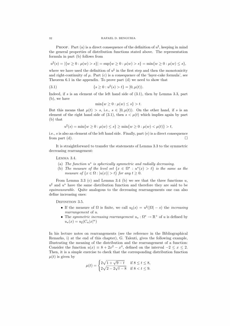
In his lecture notes on rearrangements (see the reference in the BibliographicalRemarks, i) at the end of this chapter), G. Talenti, gives the following example,illustrating the meaning of the distribution and the rearrangement of a function:Consider the function u(x) ≡ 8 + 2x2 − x4, defined on the interval −2 ≤ x ≤ 2.Then, it is a simple exercise to check that the corresponding distribution functionµ(t) is given by

µ(t) =

2√

1 +√

9− t if 8 ≤ t ≤ 8,2√

2− 2√t− 8 if 8 < t ≤ 9.


Hence,

u?(x) =

9− x2 + x4/4 if x ≤

√2,

u(x) if |x| >√

2.

This function can as well be used to illustrate the theorems below.

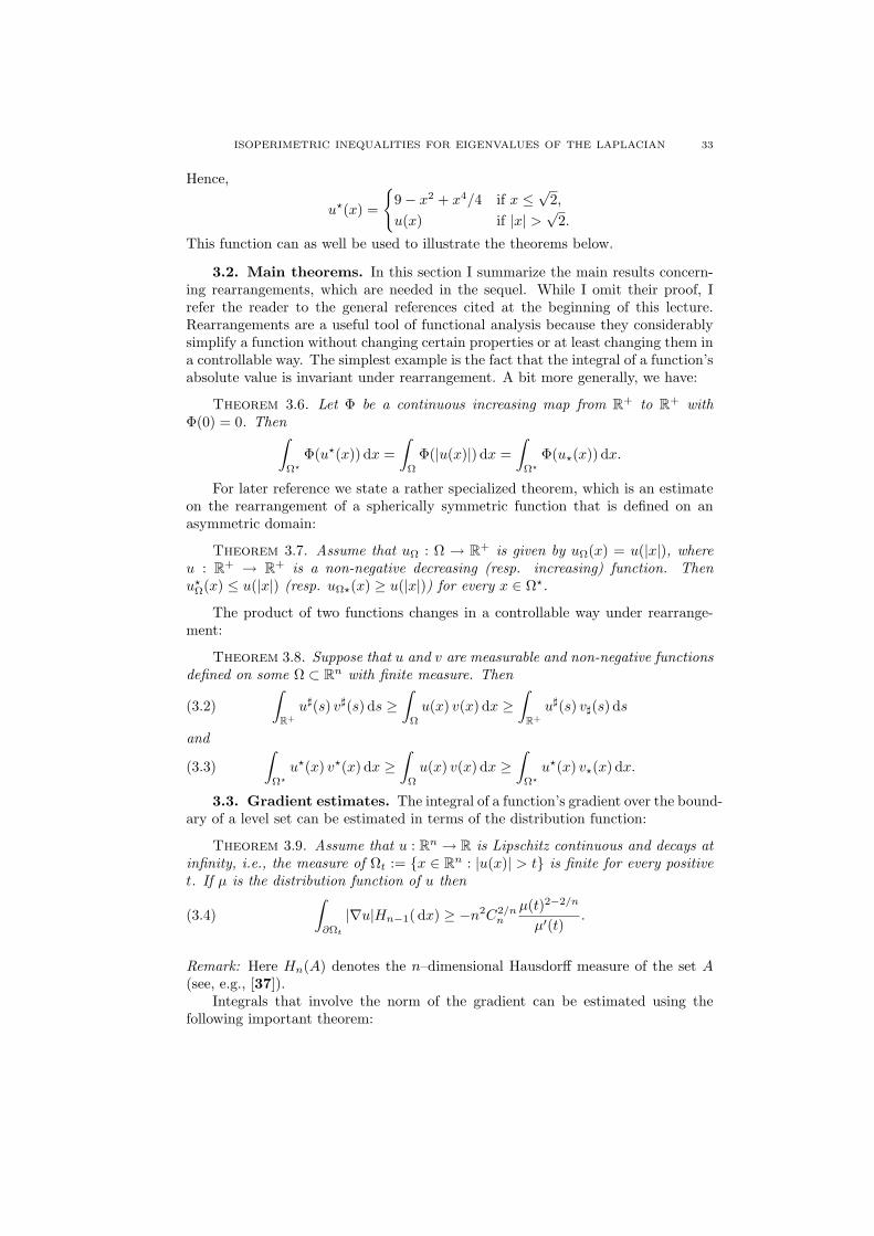
3.2. Main theorems. In this section I summarize the main results concern-ing rearrangements, which are needed in the sequel. While I omit their proof, Irefer the reader to the general references cited at the beginning of this lecture.Rearrangements are a useful tool of functional analysis because they considerablysimplify a function without changing certain properties or at least changing them ina controllable way. The simplest example is the fact that the integral of a function’sabsolute value is invariant under rearrangement. A bit more generally, we have:

Theorem 3.6. Let Φ be a continuous increasing map from R+ to R+ withΦ(0) = 0. Then∫

Ω?

Φ(u?(x)) dx =∫

Ω

Φ(|u(x)|) dx =∫

Ω?

Φ(u?(x)) dx.

For later reference we state a rather specialized theorem, which is an estimateon the rearrangement of a spherically symmetric function that is defined on anasymmetric domain:

Theorem 3.7. Assume that uΩ : Ω → R+ is given by uΩ(x) = u(|x|), whereu : R+ → R+ is a non-negative decreasing (resp. increasing) function. Thenu?Ω(x) ≤ u(|x|) (resp. uΩ?(x) ≥ u(|x|)) for every x ∈ Ω?.

The product of two functions changes in a controllable way under rearrange-ment:

Theorem 3.8. Suppose that u and v are measurable and non-negative functionsdefined on some Ω ⊂ Rn with finite measure. Then

(3.2)∫

R+u](s) v](s) ds ≥

∫Ω

u(x) v(x) dx ≥∫

R+u](s) v](s) ds

and

(3.3)∫

Ω?

u?(x) v?(x) dx ≥∫

Ω

u(x) v(x) dx ≥∫

Ω?

u?(x) v?(x) dx.

3.3. Gradient estimates. The integral of a function’s gradient over the bound-ary of a level set can be estimated in terms of the distribution function:

Theorem 3.9. Assume that u : Rn → R is Lipschitz continuous and decays atinfinity, i.e., the measure of Ωt := x ∈ Rn : |u(x)| > t is finite for every positivet. If µ is the distribution function of u then

(3.4)∫∂Ωt

|∇u|Hn−1( dx) ≥ −n2C2/nn

µ(t)2−2/n

µ′(t).

Remark: Here Hn(A) denotes the n–dimensional Hausdorff measure of the set A(see, e.g., [37]).

Integrals that involve the norm of the gradient can be estimated using thefollowing important theorem:


Theorem 3.10. Let Φ : R+ → R+ be a Young function, i.e., Φ is increasingand convex with Φ(0) = 0. Suppose that u : Rn → R is Lipschitz continuous anddecays at infinity. Then∫

Rn

Φ(|∇u?(x)|) dx ≤∫

Rn

Φ(|∇u(x)|) dx.

For the special case Φ(t) = t2 Theorem 3.10 states that the ‘energy expectationvalue’ of a function decreases under symmetric rearrangement, a fact that is key tothe proof of the Rayleigh–Faber–Krahn inequality (see Section 3.4).

Lemma 3.11. Let u and Φ be as in Theorem 3.10. Then for almost everypositive s holds

(3.5)dds

∫x∈Rn:|u(x)|>u∗(s)

Φ(|∇u|) dx ≥ Φ(−nC1/n

n s1−1/n du∗

ds(s)).

3.4. The Rayleigh–Faber–Krahn Inequality. Many isoperimetric inequal-ities have been inspired by the question which geometrical layout of some physicalsystem maximizes or minimizes a certain quantity. One may ask, for example, howmatter of a given mass density must be distributed to minimize its gravitationalenergy, or which shape a conducting object must have to maximize its electrostaticcapacity. The most famous question of this kind was put forward at the end ofthe XIXth century by Lord Rayleigh in his work on the theory of sound [65]: Heconjectured that among all drums of the same area and the same tension the circu-lar drum produces the lowest fundamental frequency. This statement was provenindependently in the 1920s by Faber [36] and Krahn [48, 49].

To treat the problem mathematically, we consider an open bounded domainΩ ⊂ R2 which matches the shape of the drum. Then the oscillation frequenciesof the drum are given by the eigenvalues of the Laplace operator −∆Ω

D on Ω withDirichlet boundary conditions, up to a constant that depends on the drum’s tensionand mass density. In the following we will allow the more general case Ω ⊂ Rn forn ≥ 2, although the physical interpretation as a drum only makes sense if n = 2.We define the Laplacian −∆Ω

D via the quadratic–form approach, i.e., it is the uniqueself–adjoint operator in L2(Ω) which is associated with the closed quadratic form

h[Ψ] =∫

Ω

|∇Ψ|2 dx, Ψ ∈ H10 (Ω).

Here H10 (Ω), which is a subset of the Sobolev space W 1,2(Ω), is the closure of

C∞0 (Ω) with respect to the form norm

(3.6) | · |2h = h[·] + || · ||L2(Ω).

For more details about the important question of how to define the Laplace operatoron arbitrary domains and subject to different boundary conditions we refer thereader to [24, 35].

The spectrum of −∆ΩD is purely discrete since H1

0 (Ω) is, by Rellich’s theorem,compactly imbedded in L2(Ω) (see, e.g., [24]). We write λ1(Ω) for the lowesteigenvalue of −∆Ω

D.


Theorem 3.12 (Rayleigh–Faber–Krahn inequality). Let Ω ⊂ Rn be an openbounded domain with smooth boundary and Ω? ⊂ Rn a ball with the same measureas Ω. Then

λ1(Ω∗) ≤ λ1(Ω)with equality if and only if Ω itself is a ball.

Proof. With the help of rearrangements at hand, the proof of the Rayleigh–Faber–Krahn inequality is actually not difficult. Let Ψ be the positive normalizedfirst eigenfunction of −∆Ω

D. Since the domain of a positive self-adjoint operator is asubset of its form domain, we have Ψ ∈ H1

0 (Ω). Then we have Ψ? ∈ H10 (Ω?). Thus

we can apply first the min–max principle and then the Theorems 3.6 and 3.10 toobtain

λ1(Ω?) ≤∫

Ω? |∇Ψ?|2 dnx∫Ω? |Ψ∗|2 dnx

≤∫

Ω|∇Ψ|2 dnx∫Ω

Ψ2 dnx= λ1(Ω).

The Rayleigh–Faber–Krahn inequality has been extended to a number of differ-ent settings, for example to Laplace operators on curved manifolds or with respectto different measures. In the following we shall give an overview of these general-izations.

3.5. Schrodinger operators. It is not difficult to extend the Rayleigh-Faber-Krahn inequality to Schrodinger operators, i.e., to operators of the form −∆+V (x).Let Ω ⊂ Rn be an open bounded domain and V : Rn → R+ a non-negative potentialin L1(Ω). Then the quadratic form

hV [u] =∫

Ω

(|∇u|2 + V (x)|u|2

)dnx,

defined on

Dom hV = H10 (Ω) ∩

u ∈ L2(Ω) :

∫Ω

(1 + V (x))|u(x)|2 dnx <∞

is closed (see, e.g., [34, 35]). It is associated with the positive self-adjoint Schrodingeroperator HV = −∆ + V (x). The spectrum of HV is purely discrete and we writeλ1(Ω, V ) for its lowest eigenvalue.

Theorem 3.13. Under the assumptions stated above,

λ1(Ω∗, V?) ≤ λ1(Ω, V ).

Proof. Let u1 ∈ Dom hV be the positive normalized first eigenfunction ofHV . Then we have u?1 ∈ H1

0 (Ω?) and by Theorem 3.8∫Ω?

(1 + V?)u?12 dnx ≤

∫Ω

(1 + V )u21 dnx <∞.

Thus u?1 ∈ Dom hV?and we can apply first the min–max principle and then Theo-

rems 3.6, 3.8 and 3.10 to obtain

λ1(Ω?, V?) ≤∫

Ω?

(|∇u?1|2 + V?u

?1

2)

dnx∫Ω? |u?1|2 dnx

≤∫

Ω

(|∇u1|2 + V u2

1

)dnx∫

Ωu2

1 dnx= λ1(Ω, V ).


3.6. Spaces of constant curvature. Differential operators can not only bedefined for functions in Euclidean space, but also for the more general case offunctions on Riemannian manifolds. It is therefore natural to ask whether theisoperimetric inequalities for the eigenvalues of the Laplacian can be generalizedto such settings as well. In this section we will state Rayleigh–Faber–Krahn typetheorems for the spaces of constant non-zero curvature, i.e., for the sphere and thehyperbolic space. Isoperimetric inequalities for the second Laplace eigenvalue inthese curved spaces will be discussed in Lecture 3.

To start with, we define the Laplacian in hyperbolic space as a self-adjointoperator by means of the quadratic form approach. We realize Hn as the open unitball B = (x1, . . . , xn) :

∑nj=1 x

2j < 1 endowed with the metric

(3.7) ds2 =4|dx|2

(1− |x|2)2

and the volume element

(3.8) dV =2n dnx

(1− |x|2)n,

where | · | denotes the Euclidean norm. Let Ω ⊂ Hn be an open domain and assumethat it is bounded in the sense that Ω does not touch the boundary of B. Thequadratic form of the Laplace operator in hyperbolic space is the closure of

(3.9) h[u] =∫

Ω

gij(∂iu)(∂ju) dV, u ∈ C∞0 (Ω).

It is easy to see that the form (3.9) is indeed closeable: Since Ω does not touchthe boundary of B, the metric coefficients gij are bounded from above on Ω. Theyare also bounded from below by gij ≥ 4. Consequently, the form norms of h andits Euclidean counterpart, which is the right hand side of (3.9) with gij replacedby δij , are equivalent. Since the ‘Euclidean’ form is well known to be closeable, hmust also be closeable.

By standard spectral theory, the closure of h induces an unique positive self-adjoint operator −∆H which we call the Laplace operator in hyperbolic space.Equivalence between corresponding norms in Euclidean and hyperbolic space im-plies that the imbedding Dom h → L2(Ω, dV ) is compact and thus the spectrumof −∆H is discrete. For its lowest eigenvalue the following Rayleigh–Faber–Krahninequality holds.

Theorem 3.14. Let Ω ⊂ Hn be an open bounded domain with smooth boundaryand Ω? ⊂ Hn an open geodesic ball of the same measure. Denote by λ1(Ω) andλ1(Ω?) the lowest eigenvalue of the Dirichlet-Laplace operator on the respectivedomain. Then

λ1(Ω?) ≤ λ1(Ω)

with equality only if Ω itself is a geodesic ball.

The Laplace operator −∆S on a domain which is contained in the unit sphereSn can be defined in a completely analogous fashion to −∆H by just replacing themetric gij in (3.9) by the metric of Sn.

Theorem 3.15. Let Ω ⊂ Sn be an open bounded domain with smooth boundaryand Ω? ⊂ Sn an open geodesic ball of the same measure. Denote by λ1(Ω) and


λ1(Ω?) the lowest eigenvalue of the Dirichlet-Laplace operator on the respectivedomain. Then

λ1(Ω?) ≤ λ1(Ω)with equality only if Ω itself is a geodesic ball.

The proofs of the above theorems are similar to the proof for the Euclideancase and will be omitted here. A more general Rayleigh–Faber–Krahn theorem forthe Laplace operator on Riemannian manifolds and its proof can be found in thebook of Chavel [31].

3.7. Robin Boundary Conditions. Yet another generalization of the Rayleigh–Faber–Krahn inequality holds for the boundary value problem

(3.10)−

n∑j=1

∂2

∂x2ju = λu in Ω,

∂u∂ν + βu = 0 on ∂Ω,

on a bounded Lipschitz domain Ω ⊂ Rn with the outer unit normal ν and someconstant β > 0. This so–called Robin boundary value problem can be interpreted asa mathematical model for a vibrating membrane whose edge is coupled elasticallyto some fixed frame. The parameter β indicates how tight this binding is andthe eigenvalues of (3.10) correspond the the resonant vibration frequencies of themembrane. They form a sequence 0 < λ1 < λ2 ≤ λ3 ≤ . . . (see, e.g., [52]).

The Robin problem (3.10) is more complicated than the corresponding Dirichletproblem for several reasons. For example, the very useful property of domainmonotonicity does not hold for the eigenvalues of the Robin–Laplacian. That is,if one enlarges the domain Ω in a certain way, the eigenvalues may go up. It isknown though, that a very weak form of domain monotonicity holds, namely thatλ1(B) ≤ λ1(Ω) if B is ball that contains Ω. Another difficulty of the Robin problem,compared to the Dirichlet case, is that the level sets of the eigenfunctions may touchthe boundary. This makes it impossible, for example, to generalize the proof of theRayleigh–Faber–Krahn inequality in a straightforward way. Nevertheless, such anisoperimetric inequality holds, as proven by Daners:

Theorem 3.16. Let Ω ⊂ Rn (n ≥ 2) be a bounded Lipschitz domain, β > 0 aconstant and λ1(Ω) the lowest eigenvalue of (3.10). Then λ1(Ω?) ≤ λ1(Ω).

For the proof of Theorem 3.16, which is not short, we refer the reader to [33].

3.8. Bibliographical Remarks. i) Rearrangements of functions were introducedby G. Hardy and J. E. Littlewood. Their results are contained in the classical book, G.H.Hardy, J. E. Littlewood, J.E., and G. Polya, Inequalities, 2d ed., Cambridge UniversityPress, 1952. The fact that the L2 norm of the gradient of a function decreases underrearrangements was proven by Faber and Krahn [36, 48, 49]. A more modern proof aswell as many results on rearrangements and their applications to PDE’s can be found in[75]. The reader may want to see also the article by E.H. Lieb, Existence and uniquenessof the minimizing solution of Choquard’s nonlinear equation, Studies in Appl. Math. 57,93–105 (1976/77), for an alternative proof of the fact that the L2 norm of the gradientdecreases under rearrangements using heat kernel techniques. An excellent expositoryreview on rearrangements of functions (with a good bibliography) can be found in Tal-enti, G., Inequalities in rearrangement invariant function spaces, in Nonlinear analysis,


function spaces and applications, Vol. 5 (Prague, 1994), 177–230, Prometheus, Prague,1994. (available at the website: http://www.emis.de/proceedings/Praha94/). The Rieszrearrangement inequality is the assertion that for nonnegative measurable functions f, g, hin Rn, we haveZ

Rn×Rn

f(y)g(x− y)h(x)dx dy ≤Z

Rn×Rn

f?(y)g?(x− y)h?(x)dx dy.

For n = 1 the inequality is due to F. Riesz, Sur une inegalite integrale, Journal of theLondon Mathematical Society 5, 162–168 (1930). For general n is due to S.L. Sobolev, Ona theorem of functional analysis, Mat. Sb. (NS) 4, 471–497 (1938) [the English translationappears in AMS Translations (2) 34, 39–68 (1963)]. The cases of equality in the Rieszinequality were studied by A. Burchard, Cases of equality in the Riesz rearrangementinequality, Annals of Mathematics 143 499–627 (1996) (this paper also has an interestinghistory of the problem).

ii) Rearrangements of functions have been extensively used to prove symmetry propertiesof positive solutions of nonlinear PDE’s. See, e.g., Kawohl, Bernhard, Rearrangementsand convexity of level sets in PDE. Lecture Notes in Mathematics, 1150. Springer-Verlag,Berlin (1985), and references therein.

iii) There are different types of rearrangements of functions. For an interesting approachto rearrangements see, Brock, Friedemann and Solynin, Alexander Yu. An approach tosymmetrization via polarization. Trans. Amer. Math. Soc. 352 1759–1796 (2000). Thisapproach goes back through Baernstein–Taylor (Duke Math. J. 1976), who cite Ahlfors(book on “Conformal invariants”, 1973), who in turn credits Hardy and Littlewood.

iv) The Rayleigh–Faber–Krahn inequality is an isoperimetric inequality concerning thelowest eigenvalue of the Laplacian, with Dirichlet boundary condition, on a boundeddomain in Rn (n ≥ 2). Let 0 < λ1(Ω) < λ2(Ω) ≤ λ3(Ω) ≤ . . . be the Dirichlet eigenvaluesof the Laplacian in Ω ⊂ Rn, i.e.,

−∆u = λu in Ω,

u = 0 on the boundary of Ω.

If n = 2, the Dirichlet eigenvalues are proportional to the square of the eigenfrequencies ofan elastic, homogeneous, vibrating membrane with fixed boundary. The Rayleigh–Faber–Krahn inequality for the membrane (i.e., n = 2) states that

λ1 ≥πj2

0,1

A,

where j0,1 = 2.4048 . . . is the first zero of the Bessel function of order zero, and A is thearea of the membrane. Equality is obtained if and only if the membrane is circular. Inother words, among all membranes of given area, the circle has the lowest fundamentalfrequency. This inequality was conjectured by Lord Rayleigh (see, [65], pp. 339–340). In1918, Courant (see R. Courant, Math. Z. 1, 321–328 (1918)) proved the weaker resultthat among all membranes of the same perimeter L the circular one yields the least lowesteigenvalue, i.e.,

λ1 ≥4π2j2

0,1

L2,

with equality if and only if the membrane is circular. Rayleigh’s conjecture was provenindependently by Faber [36] and Krahn [48]. The corresponding isoperimetric inequalityin dimension n,

λ1(Ω) ≥„

1

|Ω|

«2/n

C2/nn jn/2−1,1,


was proven by Krahn [49]. Here jm,1 is the first positive zero of the Bessel function

Jm, |Ω| is the volume of the domain, and Cn = πn/2/Γ(n/2 + 1) is the volume of then–dimensional unit ball. Equality is attained if and only if Ω is a ball. For more detailssee, R.D. Benguria, Rayleigh–Faber–Krahn Inequality, in Encyclopaedia of Mathematics,Supplement III, Managing Editor: M. Hazewinkel, Kluwer Academic Publishers, pp. 325–327, (2001).

v) A natural question to ask concerning the Rayleigh–Faber–Krahn inequality is the ques-tion of stability. If the lowest eigenvalue of a domain Ω is within ε (positive and sufficientlysmall) of the isoperimetric value λ1(Ω∗), how close is the domain Ω to being a ball? Theproblem of stability for (convex domains) concerning the Rayleigh–Faber–Krahn inequal-ity was solved by Antonios Melas (Melas, A.D., The stability of some eigenvalue esti-mates, J. Differential Geom. 36, 19–33 (1992)). In the same reference, Melas also solvedthe analogous stability problem for convex domains with respect to the PPW inequality(see Lecture 3, below). The work of Melas has been extended to the case of the Szego–Weinberger inequality (for the first nontrivial Neumann eigenvalue) by Y.-Y. Xu, The firstnonzero eigenvalue of Neumann problem on Riemannian manifolds, J. Geom. Anal. 5151–165 (1995), and to the case of the PPW inequality on spaces of constant curvatureby A. Avila, Stability results for the first eigenvalue of the Laplacian on domains in spaceforms, J. Math. Anal. Appl. 267, 760–774 (2002). In this connection it is worth mention-ing related results on the isoperimetric inequality of R. Hall, A quantitative isoperimetricinequality in n–dimensional space, J. Reine Angew Math. 428 , 161–176 (1992), as well asrecent results of Maggi, Pratelli and Fusco (recently reviewed by F. Maggi in Bull. Amer.Math. Soc. 45, 367–408 (2008).

vi) The analog of the Faber–Krahn inequality for domains in the sphere Sn was proven bySperner, Emanuel, Jr. Zur Symmetrisierung von Funktionen auf Spharen, Math. Z. 134,317–327 (1973).

vii) For isoperimetric inequalities for the lowest eigenvalue of the Laplace–Beltrami op-erator on manifolds, see, e.g., the book by Chavel, Isaac, Eigenvalues in Riemanniangeometry. Pure and Applied Mathematics, 115. Academic Press, Inc., Orlando, FL,1984, (in particular Chapters IV and V), and also the articles, Chavel, I. and Feldman,E. A. Isoperimetric inequalities on curved surfaces. Adv. in Math. 37, 83–98 (1980),and Bandle, Catherine, Konstruktion isoperimetrischer Ungleichungen der mathematis-chen Physik aus solchen der Geometrie, Comment. Math. Helv. 46, 182–213 (1971).

viii) Recently, the analog of the Rayleigh–Faber–Krahn inequality for an elliptic operatorwith drift was proven by F. Hamel, N. Nadirashvili and E. Russ [41]. In fact, let Ωbe a bounded C2,α domain in Rn (with n ≥ 1 and 0 < α < 1), and τ ≥ 0. Let ~v ∈L∞(Ω,Rn), with ‖v‖∞ ≤ τ . Let λ1(Ω, v) denote the principal eigenvalue of −∆ + ~v · ∇with Dirichlet boundary conditions. Then, λ1(Ω, ~v) ≥ λ1(Ω∗, τ er), where er = x/|x|.Moreover, equality is attained up to translations, if and only if Ω = Ω∗ and ~v = τ er.See, F. Hamel, N. Nadirashvili, and E. Russ, Rearrangement inequalities and applicationsto isoperimetric problems for eigenvalues, to appear in Annals of Mathematics (2011)(and references therein), where the authors develop a new type of rearrangement to provethis and many other isoperimetric results for the class of elliptic operators of the form−div(A · ∇) + v · ∇ + V , with Dirichlet boundary conditions, in Ω. Here A is a positivedefinite matrix.


4. Lecture 3: The Szego–Weinberger and the Payne–Polya–Weinbergerinequalities

4.1. The Szego–Weinberger inequality. In analogy to the Rayleigh–Faber–Krahn inequality for the Dirichlet–Laplacian one may ask which shape of a domainmaximizes certain eigenvalues of the Laplace operator with Neumann boundaryconditions. Of course, this question is trivial for the lowest Neumann eigenvalue,which is always zero. In 1952 Kornhauser and Stakgold [47] conjectured that theball maximizes the first non-zero Neumann eigenvalue among all domains of thesame volume. This was first proven in 1954 by Szego [72] for two-dimensional sim-ply connected domains, using conformal mappings. Two years later his result wasgeneralized to domains in any dimension by Weinberger [76], who came up with anew strategy for the proof.

Although the Szego–Weinberger inequality appears to be the analog for Neu-mann eigenvalues of the Rayleigh–Faber–Krahn inequality, its proof is completelydifferent. The reason is that the first non-trivial Neumann eigenfunction must beorthogonal to the constant function, and thus it must have a change of sign. Thesimple symmetrization procedure that is used to establish the Rayleigh–Faber–Krahn inequality can therefore not work.

In general, when dealing with Neumann problems, one has to take into accountthat the spectrum of the respective Laplace operator on a bounded domain isvery unstable under perturbations. One can change the spectrum arbitrarily muchby only a slight modification of the domain, and if the boundary is not smoothenough, the Laplacian may even have essential spectrum. A sufficient condition forthe spectrum of −∆Ω

N to be purely discrete is that Ω is bounded and has a Lipschitzboundary [35]. We write 0 = µ0(Ω) < µ1(Ω) ≤ µ2(Ω) ≤ . . . for the sequence ofNeumann eigenvalues on such a domain Ω.

Theorem 4.1 (Szego–Weinberger inequality). Let Ω ⊂ Rn be an open boundeddomain with smooth boundary such that the Laplace operator on Ω with Neumannboundary conditions has purely discrete spectrum. Then

(4.1) µ1(Ω) ≤ µ1(Ω?),

where Ω? ⊂ Rn is a ball with the same n-volume as Ω. Equality holds if and onlyif Ω itself is a ball.

Proof. By a standard separation of variables one shows that µ1(Ω?) is n-folddegenerate and that a basis of the corresponding eigenspace can be written in theform g(r)rjr−1j=1,...,n. The function g can be chosen to be positive and satisfiesthe differential equation

(4.2) g′′ +n− 1r

g′ +(µ1(Ω?)− n− 1

r2

)g = 0, 0 < r < R1,

where R1 is the radius of Ω?. Further, g(r) vanishes at r = 0 and its derivative hasits first zero at r = R1. We extend g by defining g(r) = limr′↑R1 g(r′) for r ≥ R1.Then g is differentiable on R and if we set fj(~r) := g(r)rjr−1 then fj ∈W 1,2(Ω) forj = 1 . . . , n. To apply the min-max principle with fj as a test function for µ1(Ω)we have to make sure that fj is orthogonal to the first (trivial) eigenfunction, i.e.,that

(4.3)∫

Ω

fj dnr = 0, j = 1, . . . , n.


We argue that this can be achieved by some shift of the domain Ω: Since Ω isbounded we can find a ball B that contains Ω. Now define the vector field ~b : Rn →Rn by its components

bj(~v) =∫

Ω+~v

fj(~r) dnr, ~v ∈ Rn.

For ~v ∈ ∂B we have

~v ·~b(~v) =∫

Ω+~v

~v · ~rrg(r) dnr

=∫

Ω

~v · (~r + ~v)|~r + ~v|

g(|~r + ~v|) dnr

≥∫

Ω

|~v|2 − |v| · |r||~r + ~v|

g(|~r + ~v|) dnr > 0.

Thus~b is a vector field that points outwards on every point of ∂B. By an applicationof the Brouwer’s fixed–point theorem (see Theorem 6.3 in the Appendix) this meansthat ~b(~v0) = 0 for some ~v0 ∈ B. Thus, if we shift Ω by this vector, condition (4.3)is satisfied and we can apply the min-max principle with the fj as test functionsfor the first non-zero eigenvalue:

µ1(Ω) ≤∫

Ω|∇fj |dnr∫Ωf2j dnr

=

∫Ω

(g′

2(r)r2j r−2 + g2(r)(1− r2

j r−2)r−2

)dnr∫

Ωg2r2

j r−2 dnr

.

We multiply each of these inequalities by the denominator and sum up over j toobtain

(4.4) µ1(Ω) ≤∫

ΩB(r) dnr∫

Ωg2(r) dnr

with B(r) = g′2(r) + (n− 1)g2(r)r−2. Since R1 is the first zero of g′, the function

g is non-decreasing. The derivative of B is

B′ = 2g′g′′ + 2(n− 1)(rgg′ − g2)r−3.

For r ≥ R1 this is clearly negative since g is constant there. For r < R1 we can useequation (4.2) to show that

B′ = −2µ1(Ω?)gg′ − (n− 1)(rg′ − g)2r−3 < 0.

In the following we will use the method of rearrangements, which was described inChapter 3. To avoid confusions, we use a more precise notation at this point: Weintroduce BΩ : Ω→ R , BΩ(~r ) = B(r) and analogously gΩ : Ω→ R, gΩ(~r ) = g(r).Then equation (4.4) yields, using Theorem 3.7 in the third step:

(4.5) µ1(Ω) ≤∫

ΩBΩ(~r ) dnr∫

Ωg2

Ω(~r ) dnr=

∫Ω? B

?Ω(~r ) dnr∫

Ω? g2?Ω(~r ) dnr

≤∫

Ω? B(r) dnr∫Ω? g2(r) dnr

= µ1(Ω?)

Equality holds obviously if Ω is a ball. In any other case the third step in (4.5) isa strict inequality.


It is rather straightforward to generalize the Szego–Weinberger inequality todomains in hyperbolic space. For domains on spheres, on the other hand, thecorresponding inequality has not been established yet in full generality. At present,the most general result is due to Ashbaugh and Benguria: In [9] they show that ananalog of the Szego–Weinberger inequality holds for domains that are contained ina hemisphere.

4.2. The Payne–Polya–Weinberger inequality. A further isoperimetricinequality is concerned with the second eigenvalue of the Dirichlet–Laplacian onbounded domains. In 1955 Payne, Polya and Weinberger (PPW) showed that forany open bounded domain Ω ⊂ R2 the bound λ2(Ω)/λ1(Ω) ≤ 3 holds [60, 61].Based on exact calculations for simple domains they also conjectured that the ratioλ2(Ω)/λ1(Ω) is maximized when Ω is a circular disk, i.e., that

(4.6)λ2(Ω)λ1(Ω)

≤ λ2(Ω?)λ1(Ω?)

=j21,1

j20,1

≈ 2.539 for Ω ⊂ R2.

Here, jn,m denotes the mth positive zero of the Bessel function Jn(x). This con-jecture and the corresponding inequalities in n dimensions were proven in 1991 byAshbaugh and Benguria [6, 7, 8]. Since the Dirichlet eigenvalues on a ball areinversely proportional to the square of the ball’s radius, the ratio λ2(Ω?)/λ1(Ω?)does not depend on the size of Ω?. Thus we can state the PPW inequality in thefollowing form:

Theorem 4.2 (Payne–Polya–Weinberger inequality). Let Ω ⊂ Rn be an openbounded domain and S1 ⊂ Rn a ball such that λ1(Ω) = λ1(S1). Then

(4.7) λ2(Ω) ≤ λ2(S1)

with equality if and only if Ω is a ball.

Here the subscript 1 on S1 reflects the fact that the ball S1 has the same firstDirichlet eigenvalue as the original domain Ω. The inequalities (4.6) and (4.7) areequivalent in Euclidean space in view of the mentioned scaling properties of theeigenvalues. Yet when one considers possible extensions of the PPW inequality toother settings, where λ2/λ1 varies with the radius of the ball, it turns out that anestimate in the form of Theorem 4.2 is the more natural result. In the case of adomain on a hemisphere, for example, λ2/λ1 on balls is an increasing function ofthe radius. But by the Rayleigh–Faber–Krahn inequality for spheres the radius ofS1 is smaller than the one of the spherical rearrangement Ω?. This means that anestimate in the form of Theorem 4.2, interpreted as

λ2(Ω)λ1(Ω)

≤ λ2(S1)λ1(S1)

, Ω, S1 ⊂ Sn,

is stronger than an inequality of the type (4.6).On the other hand, we will see that in the hyperbolic space λ2/λ1 on balls is

a strictly decreasing function of the radius. In this case we can apply the follow-ing argument to see that an estimate of the type (4.6) cannot possibly hold true:Consider a domain Ω that is constructed by attaching very long and thin tentaclesto the ball B. Then the first and second eigenvalues of the Laplacian on Ω arearbitrarily close to the ones on B. The spherical rearrangement of Ω though can


be considerably larger than B. This means thatλ2(Ω)λ1(Ω)

≈ λ2(B)λ1(B)

>λ2(Ω?)λ1(Ω?)

, B,Ω ⊂ Hn,

clearly ruling out any inequality in the form of (4.6).The proof of the PPW inequality (4.7) is somewhat similar to that of the Szego–

Weinberger inequality (see the previous section in this Lecture), but considerablymore difficult. The additional complications mainly stem from the fact that in theDirichlet case the first eigenfunction of the Laplacian is not known explicitly, whilein the Neumann case it is just constant. We will give the full proof of the PPWinequality in the sequel. Since it is rather long, a brief outline is in order:

The proof is organized in six steps. In the first one we use the min–max principleto derive an estimate for the eigenvalue gap λ2(Ω) − λ1(Ω), depending on a testfunction for the second eigenvalue. In the second step we define such a function andthen show in the third step that it actually satisfies all requirements to be used inthe gap formula. In the fourth step we put the test function into the gap inequalityand then estimate the result with the help of rearrangement techniques. Thesedepend on the monotonicity properties of two functions g and B, which are to bedefined in the proof, and on a Chiti comparison argument. The later is a specialcomparison result which establishes a crossing property between the symmetricdecreasing rearrangement of the first eigenfunction on Ω and the first eigenfunctionon S1. We end up with the inequality λ2(Ω)−λ1(Ω) ≤ λ2(S1)−λ1(S1), which yields(4.7). In the remaining two steps we prove the mentioned monotonicity propertiesand the Chiti comparison result. We remark that from the Rayleigh–Faber–Krahninequality follows S1 ⊂ Ω?, a fact that is used in the proof of the Chiti comparisonresult. Although it enters in a rather subtle manner, the Rayleigh–Faber–Krahninequality is an important ingredient of the proof of the PPW inequality.

4.3. Proof of the Payne–Polya–Weinberger inequality. First step: Wederive the ‘gap formula’ for the first two eigenvalues of the Dirichlet–Laplacian onΩ. We call u1 : Ω → R+ the positive normalized first eigenfunction of −∆D

Ω . Toestimate the second eigenvalue we will use the test function Pu1, where P : Ω→ Ris is chosen such that Pu1 is in the form domain of −∆D

Ω and

(4.8)∫

Ω

Pu21 drn = 0.

Then we conclude from the min–max principle that

λ2(Ω)− λ1(Ω) ≤∫

Ω

(|∇(Pu1)|2 − λ1P

2u21

)drn∫

ΩP 2u2

1 drn

=

∫Ω

(|∇P |2u2

1 + (∇P 2)u1∇u1 + P 2|∇u1|2 − λ1P2u2

1

)drn∫

ΩP 2u2

1 drn(4.9)

If we perform an integration by parts on the second summand in the numeratorof (4.9), we see that all summands except the first cancel. We obtain the gapinequality

(4.10) λ2(Ω)− λ1(Ω) ≤∫

Ω|∇P |2u2

1 drn∫ΩP 2u2

1 drn.

Second step: We need to fix the test function P . Our choice will be dictatedby the requirement that equality should hold in (4.10) if Ω is a ball, i.e., if Ω = S1


up to translations. We assume that S1 is centered at the origin of our coordinatesystem and call R1 its radius. We write z1(r) for the first eigenfunction of theDirichlet Laplacian on S1. This function is spherically symmetric with respectto the origin and we can take it to be positive and normalized in L2(S1). Thesecond eigenvalue of −∆D

S1in n dimensions is n–fold degenerate and a basis of the

corresponding eigenspace can be written in the form z2(r)rjr−1 with z2 ≥ 0 andj = 1, . . . , n. This is the motivation to choose not only one test function P , butrather n functions Pj with j = 1, . . . , n. We set

Pj = rjr−1g(r)

with

g(r) =

z2(r)z1(r) for r < R1,

limr′↑R1z2(r′)z1(r′) for r ≥ R1.

We note that Pju1 is a second eigenfunction of −∆DΩ if Ω is a ball which is centered

at the origin.Third step: It is necessary to verify that the Pju1 are admissible test functions.

First, we have to make sure that condition (4.8) is satisfied. We note that Pjchanges when Ω (and u1 with it) is shifted in Rn. Since these shifts do not changeλ1(Ω) and λ2(Ω), it is sufficient to show that Ω can be moved in Rn such that (4.8)is satisfied for all j ∈ 1, . . . , n. To this end we define the function

~b(~v) =∫

Ω+~v

u21(|~r − ~v |)~r

rg(r) drn for ~v ∈ Rn.

Since Ω is a bounded domain, we can choose some closed ball D, centered at theorigin, such that Ω ⊂ D. Then for every ~v ∈ ∂D we have

~v ·~b(~v) =∫

Ω

~v · u21(r)

~r + ~v

|~r + ~v |g(|~r + ~v |) drn

>

∫Ω

u21(r)|~v|2 − |~v| · |~r ||~r + ~v |

g(|~r + ~v |) drn > 0

Thus the continuous vector-valued function ~b(~v ) points strictly outwards every-where on ∂D. By Theorem 6.3, which is a consequence of the Brouwer fixed–pointtheorem, there is some ~v0 ∈ D such that ~b(~v0) = 0. Now we shift Ω by this vector,i.e., we replace Ω by Ω−~v0 and u1 by the first eigenfunction of the shifted domain.Then the test functions Pju1 satisfy the condition (4.8).

The second requirement on Pju1 is that it must be in the form domain of−∆D

Ω , i.e., in H10 (Ω): Since u1 ∈ H1

0 (Ω) there is a sequence vn ∈ C1(Ω)n∈Nof functions with compact support such that | · |h − limn→∞ vn = u1, using thedefinition (3.6) of | · |h. The functions Pjvn also have compact support and one cancheck that Pjvn ∈ C1(Ω) (Pj is continuously differentiable since g′(R1) = 0). Wehave | · |h − limn→∞ Pjvn = Pju1 and thus Pju1 ∈ H1

0 (Ω).Fourth step: We multiply the gap inequality (4.10) by

∫P 2u2

1 dx and put inour special choice of Pj to obtain

(λ2 − λ1)∫

Ω

r2j

r2g2(r)u2

1(r) drn ≤∫

Ω

∣∣∣∇(rjrg(r)

)∣∣∣2 u21(r) drn

=∫

Ω

(∣∣∣∇rjr

∣∣∣2 g2(r) +r2j

r2g′(r)2

)u2

1(r) drn.


Now we sum these inequalities up over j = 1, . . . , n and then divide again by theintegral on the left hand side to get

(4.11) λ2(Ω)− λ1(Ω) ≤∫

ΩB(r)u2

1(r) drn∫Ωg2(r)u2

1(r) drn

with

(4.12) B(r) = g′(r)2 + (n− 1)r−2g(r)2.

In the following we will use the method of rearrangements, which was described inthe second Lecture. To avoid confusions, we use a more precise notation at thispoint: We introduce BΩ : Ω → R , BΩ(~r) = B(r) and analogously gΩ : Ω → R,gΩ(~r) = g(r). Then equation (4.11) can be written as

(4.13) λ2(Ω)− λ1(Ω) ≤∫

ΩBΩ(~r)u2

1(~r) drn∫Ωg2

Ω(~r)u21(~r) drn

.

Then by Theorem 3.8 the following inequality is also true:

(4.14) λ2(Ω)− λ1(Ω) ≤∫

Ω? B?Ω(~r)u?1(~r)2 drn∫

Ω? g2Ω?(~r)u

?1(~r)2 drn

.

Next we use the very important fact that g(r) is an increasing function and B(r) isa decreasing function, which we will prove in step five below. These monotonicityproperties imply by Theorem 3.7 that B?Ω(~r) ≤ B(r) and gΩ?(~r) ≥ g(r). Therefore

(4.15) λ2(Ω)− λ1(Ω) ≤∫

Ω? B(r)u?1(r)2 drn∫Ω? g2(r)u?1(r)2 drn

.

Finally we use the following version of Chiti’s comparison theorem to estimate theright hand side of (4.15):

Lemma 4.3 (Chiti comparison result). There is some r0 ∈ (0, R1) such that

z1(r) ≥ u?1(r) for r ∈ (0, r0) andz1(r) ≤ u?1(r) for r ∈ (r0, R1).

We remind the reader that the function z1 denotes the first Dirichlet eigenfunc-tion for the Laplacian defined on S1. Applying Lemma 4.3, which will be provenbelow in step six, to (4.15) yields

(4.16) λ2(Ω)− λ1(Ω) ≤∫

Ω? B(r)z1(r)2 drn∫Ω? g2(r)z1(r)2 drn

= λ2(S1)− λ1(S1).

Since S1 was chosen such that λ1(Ω) = λ1(S1) the above relation proves thatλ2(Ω) ≤ λ2(S1). It remains the question: When does equality hold in (4.7)? It isobvious that equality does hold if Ω is a ball, since then Ω = S1 up to translations.On the other hand, if Ω is not a ball, then (for example) the step from (4.15) to(4.16) is not sharp. Thus (4.7) is a strict inequality if Ω is not a ball.

4.4. Monotonicity of B and g. Fifth step: We prove that g(r) is an in-creasing function and B(r) is a decreasing function. In this step we abbreviateλi = λi(S1). The functions z1 and z2 are solutions of the differential equations

−z′′1 −n− 1r

z′1 − λ1z1 = 0,(4.17)

−z′′2 −n− 1r

z′2 +(n− 1r2− λ2

)z2 = 0


with the boundary conditions

(4.18) z′1(0) = 0, z1(R1) = 0, z2(0) = 0, z2(R1) = 0.

We define the function

(4.19) q(r) :=

rg′(r)g(r) for r ∈ (0, R1),

limr′↓0 q(r′) for r = 0,limr′↑R1 q(r

′) for r = R1.

Proving the monotonicity of B and g is thus reduced to showing that 0 ≤ q(r) ≤ 1and q′(r) ≤ 0 for r ∈ [0, R1]. Using the definition of g and the equations (4.17),one can show that q(r) is a solution of the Riccati differential equation

(4.20) q′ = (λ1 − λ2)r +(1− q)(q + n− 1)

r− 2q

z′1z1.

It is straightforward to establish the boundary behavior

q(0) = 1, q′(0) = 0, q′′(0) =2n

((1 +

2n

)λ1 − λ2

)and

q(R1) = 0.

Lemma 4.4. For 0 ≤ r ≤ R1 we have q(r) ≥ 0.

Proof. Assume the contrary. Then there exist two points 0 < s1 < s2 ≤ R1

such that q(s1) = q(s2) = 0 but q′(s1) ≤ 0 and q′(s2) ≥ 0. If s2 < R1 then theRiccati equation (4.20) yields

0 ≥ q′(s1) = (λ1 − λ2)s1 +n− 1s1

> (λ1 − λ2)s2 +n− 1s2

= q′(s2) ≥ 0,

which is a contradiction. If s2 = R1 then we get a contradiction in a similar wayby

0 ≥ q′(s1) = (λ1 − λ2)s1 +n− 1s1

> (λ1 − λ2)R1 +n− 1R1

= 3q′(R1) ≥ 0.

In the following we will analyze the behavior of q′ according to (4.20), consid-ering r and q as two independent variables. For the sake of a compact notation wewill make use of the following abbreviations:

p(r) = z′1(r)/z1(r)Ny = y2 − n+ 1

Qy = 2yλ1 + (λ2 − λ1)Nyy−1 − 2(λ2 − λ1)

My = N2y /(2y)− (n− 2)2y/2

We further define the function

(4.21) T (r, y) := −2p(r)y − (n− 2)y +Nyr

− (λ2 − λ1)r.

Then we can write (4.20) as

q′(r) = T (r, q(r)).


The definition of T (r, y) allows us to analyze the Riccati equation for q′ consideringr and q(r) as independent variables. For r going to zero, p is O(r) and thus

T (r, y) =1r

((n− 1 + y)(1− y)) +O(r) for y fixed.

Consequently,

limr→0 T (r, y) = +∞ for 0 ≤ y < 1 fixed,limr→0 T (r, y) = 0 for y = 1 andlimr→0 T (r, y) = −∞ for y > 1 fixed.

The partial derivative of T (r, y) with respect to r is given by

(4.22) T ′ =∂

∂rT (r, y) = −2yp′ +

(n− 2)yr2

+Nyr2− (λ2 − λ1).

In the points (r, y) where T (r, y) = 0 we have, by (4.21),

(4.23) p|T=0 = −n− 22r− Ny

2yr− (λ2 − λ1)r

2y.

From (4.17) we get the Riccati equation

(4.24) p′ + p2 +n− 1r

p+ λ1 = 0.

Putting (4.23) into (4.24) and the result into (4.22) yields

(4.25) T ′|T=0 =My

r2+

(λ2 − λ1)2

2yr2 +Qy.

Lemma 4.5. There is some r0 > 0 such that q(r) ≤ 1 for all r ∈ (0, r0) andq(r0) < 1.

Proof. Suppose the contrary, i.e., q(r) first increases away from r = 0. Then,because q(0) = 1 and q(R1) = 0 and because q is continuous and differentiable, wecan find two points s1 < s2 such that q := q(s1) = q(s2) > 1 and q′(s1) > 0 > q′(s2).Even more, we can chose s1 and s2 such that q is arbitrarily close to one. Writingq = 1 + ε with ε > 0, we can calculate from the definition of Qy that

Q1+ε = Q1 + εn (λ2 − (1− 2/n)λ1) +O(ε2).

The term in brackets can be estimated by

λ2 − (1− 2/n)λ1 > λ2 − λ1 > 0.

We can also assume that Q1 ≥ 0, because otherwise q′′(0) = 2n2Q1 < 0 and Lemma

4.5 is immediately true. Thus, choosing R1 and r2 such that ε is sufficiently small,we can make sure that Qq > 0.

Now consider T (r, q) as a function of r for our fixed q. We have T (s1, q) > 0 >T (s2, q) and the boundary behavior T (0, q) = −∞. Consequently, T (r, q) changesits sign at least twice on [0, R1] and thus we can find two zeros 0 < s1 < s2 < R1

of T (r, q) such that

(4.26) T ′(s1, q) ≥ 0 and T ′(s2, q) ≤ 0.

But from (4.25), together with Qq > 0, one can see easily that this is impossible,because the right hand side of (4.25) is either positive or increasing (depending onMq). This is a contradiction to our assumption that q first increases away fromr = 0, proving Lemma 4.5.


Lemma 4.6. For all 0 ≤ r ≤ R1 the inequality q′(r) ≤ 0 holds.

Proof. Assume the contrary. Then, because of q(0) = 1 and q(R1) = 0, thereare three points s1 < s2 < s3 in (0, R1) with 0 < q := q(s1) = q(s2) = q(s3) < 1 andq′(s1) < 0, q′(s2) > 0, q′(s3) < 0. Consider the function T (r, q), which coincideswith q′(r) at s1, s2, s3. Taking into account its boundary behavior at r = 0, it isclear that T (r, q) must have at least the sign changes positive-negative-positive-negative. Thus T (r, q) has at least three zeros s1 < s2 < s3 with the properties

T ′(s1, q) ≤ 0, T ′(s2, q) ≥ 0, T ′(s3, q) ≤ 0.

Again one can see from (4.25) that this is impossible, because the term on theright hand side is either a strictly convex or a strictly increasing function of r. Weconclude that Lemma 4.6 is true.

Altogether we have shown that 0 ≤ q(r) ≤ 1 and q′(r) ≤ 0 for all r ∈ (0, R1),which proves that g is increasing and B is decreasing.

4.5. The Chiti comparison result. Sixth step: We prove Lemma 4.3: Hereand in the sequel we write short-hand λ1 = λ1(Ω) = λ1(S1). We introduce a changeof variables via s = Cnr

n, where Cn is the volume of the n–dimensional unit ball.Then by Definition 3.2 we have u]1(s) = u?1(r) and z]1(s) = z1(r).

Lemma 4.7. For the functions u]1(s) and z]1(s) we have

− du]1ds

≤ λ1n−2C−2/n

n sn/2−2

∫ s

0

u]1(w) dw,(4.27)

− dz]1ds

= λ1n−2C−2/n

n sn/2−2

∫ s

0

z]1(w) dw.(4.28)

Proof. We integrate both sides of −∆u1 = λ1u1 over the level set Ωt := ~r ∈Ω : u1(~r) > t and use Gauss’ Divergence Theorem to obtain

(4.29)∫∂Ωt

|∇u1|Hn−1( dr) =∫

Ωt

λ1 u1(~r) dnr,

where ∂Ωt = ~r ∈ Ω : u1(~r) = t. Now we define the distribution function µ(t) =|Ωt|. Then by Theorem 3.9 we have

(4.30)∫∂Ωt

|∇u1|Hn−1( dr) ≥ −n2C2/nn

µ(t)2−2/n

µ′(t).

The left sides of (4.29) and (4.30) are the same, thus

−n2C2/nn

µ(t)2−2/n

µ′(t)≤

∫Ωt

λ1 u1(~r) dnr

=∫ (µ(t)/Cn)1/n

0

nCnrn−1λ1u

?1(r) dr.

Now we perform the change of variables r → s on the right hand side of the abovechain of inequalities. We also chose t to be u]1(s). Using the fact that u]1 andµ are essentially inverse functions to one another, this means that µ(t) = s andµ′(t)−1 = (u]1)′(s). The result is (4.27). Equation (4.28) is proven analogously,with equality in each step.


Lemma 4.7 enables us to prove Lemma 4.3. The function z]1 is continuous on(0, |S1|) and u]1 is continuous on (0, |Ω?|). By the normalization of u]1 and z]1 andbecause S1 ⊂ Ω? it is clear that either z]1 ≥ u]1 on (0, |S1|) or u]1 and z]1 have atleast one intersection on this interval. In the first case there is nothing to prove,simply setting r0 = R1 in Lemma 4.3. In the second case we have to show thatthere is no intersection of u]1 and z]1 such that u]1 is greater than z]1 on the left andsmaller on the right. So we assume the contrary, i.e., that there are two points0 ≤ s1 < s2 < |S1| such that u]1(s) > z]1(s) for s ∈ (s1, s2), u]1(s2) = z]1(s2) andeither u]1(s1) = z]1(s1) or s1 = 0. We set

(4.31) v](s) =

u]1(s) on [0, s1] if

∫ s10u]1(s) ds >

∫ s10z]1(s) ds,

z]1(s) on [0, s1] if∫ s1

0u]1(s) ds ≤

∫ s10z]1(s) ds,

u]1(s) on [s1, s2],z]1(s) on [s2, |S1|].

Then one can convince oneself that because of (4.27) and (4.28)

(4.32) − dv]

ds≤ λ1n

−2C−2/nn sn/2−2

∫ s

0

v](s′) ds′

for all s ∈ [0, |S1|]. Now define the test function v(r) = v](Cnrn). Using theRayleigh–Ritz characterization of λ1, then (4.32) and finally an integration by parts,we get (if z1 and u1 are not identical)

λ1

∫S1

v2(r) dnx <

∫S1

|∇v|2 dnx =∫ |S1|

0

(nCnr

n−1 v]′(s))2 ds

≤ −∫ |S1|

0

v]′(s)λ1

∫ s

0

v](s′) ds′ ds

= λ1

∫ |S1|

0

v](s)2 ds− λ1

[v](s)

∫ s

0

v](s′) ds′] ∣∣∣S1

0

≤ λ1

∫S1

v2(r) dnx

Comparing the first and the last term in the above chain of (in)equalities reveals acontradiction to our assumption that the intersection point s2 exists, thus provingLemma 4.3.

4.6. Schrodinger operators. Theorem 4.2 can be extended in several direc-tions. One generalization, which has been considered by Benguria and Linde in[18], is to replace the Laplace operator on the domain Ω ⊂ Rn by a Schrodingeroperator H = −∆ + V . In this case the question arises which is the most suitablecomparison operator for H. In analogy to the PPW inequality for the Laplacian, itseems natural to compare the eigenvalues of H to those of another Schrodinger op-erator H = −∆ + V , which is defined on a ball and has the same lowest eigenvalueas H. The potential V should be spherically symmetric and it should reflect someproperties of V , but it will also have to satisfy certain requirements in order forthe PPW type estimate to hold. The precise result is stated in Theorem 4.8 below,which can be considered as a natural generalization of Theorem 4.2 to Schrodingeroperators.


We assume that Ω is open and bounded and that V : Ω→ R+ is a non-negativepotential from L1(Ω). Then we can define the Schrodinger operator HV = −∆ +Von Ω in the same way as we did in Section 3.5, i.e., HV is positive and self-adjointin L2(Ω) and has purely discrete spectrum. We call λi(Ω, V ) its i-th eigenvalueand, as usual, we write V? for the symmetric increasing rearrangement of V .

Theorem 4.8. Let S1 ⊂ Rn be a ball centered at the origin and of radius R1

and let V : S1 → R+ be a radially symmetric non-negative potential such thatV (r) ≤ V?(r) for all 0 ≤ r ≤ R1 and λ1(Ω, V ) = λ1(S1, V ). If V (r) satisfies theconditions

a) V (0) = V ′(0) = 0 andb) V ′(r) exists and is increasing and convex,

then

(4.33) λ2(Ω, V ) ≤ λ2(S1, V ).

If V is such that V? itself satisfies the conditions a) and b) of the theorem, thebest bound is obtained by choosing V = V? and then adjusting the size of S1 suchthat λ1(Ω, V ) = λ1(S1, V?) holds. (Note that S1 ⊂ Ω? by Theorem 3.13). In thiscase Theorem 4.8 is a typical PPW result and optimal in the sense that equalityholds in (4.33) if Ω is a ball and V = V?. For a general potential V we still get anon-trivial bound on λ2(Ω, V ) though it is not sharp anymore.

For further reference we state the following theorem, which is a direct conse-quence of Theorem 4.8 and Theorem 3.7:

Theorem 4.9. Let V : Rn → R+ be a radially symmetric positive potential thatsatisfies the conditions a) and b) of Theorem 4.2. Further, assume that Ω ⊂ Rn isan open bounded domain and that S1 ⊂ Rn be the open ball (centered at the origin)such that λ1(Ω, V ) = λ1(S1, V ). Then

λ2(Ω, V ) ≤ λ2(S1, V ).

The proof of Theorem 4.8 is similar to the one of Theorem 4.2 and can be foundin [18]. One of the main differences occurs in step five (see Section 4.4), since thepotential V (r) now appears in the Riccati equation for p. It turns out that theconditions a) and b) in Theorem 4.8 are required to establish the monotonicityproperties of q. A second important difference is that a second eigenfunction ofa Schrodinger operator with a spherically symmetric potential can not necessarilybe written in the form u2(r)rjr−1. It has been shown by Ashbaugh and Benguria[5] that it can be written in this form if rV (r) is convex. On the other hand, thesecond eigenfunction is radially symmetric (with a spherical nodal surface) if rV (r)is concave. This fact, which is also known as the Baumgartner–Grosse–MartinInequality [17], is another reason why the conditions a) and b) of Theorem 4.8 areneeded.

4.7. Spaces of constant curvature. There are generalizations of the Payne-Polya-Weinberger inequality to spaces of constant curvature. Ashbaugh and Ben-guria showed in [11] that Theorem 4.2 remains valid if one replaces the Euclideanspace Rn by a hemisphere of Sn and ‘ball’ by ‘geodesic ball’. Similar to theSzego–Weinberger inequality, it is still an open problem to prove a Payne–Polya–Weinberger result for the whole sphere. Although there seem to be no counterex-amples known that rule out such a generalization, the original scheme of proving


the PPW inequality is not likely to work. One reason is that numerical studiesshow the function g to be not monotone on the whole sphere.

For the hyperbolic space, on the other hand, things are settled. Following thegeneral lines of the original proof, Benguria and Linde established in [19] a PPWtype inequality that holds in any space of constant negative curvature.

4.8. Bibliographical Remarks. i) In 1952, Kornhauser and Stakgold [47] conjec-tured that the lowest nontrivial Neumann eigenvalue for a smooth bounded domain Ω inR2 satisfies the isoperimetric inequality

µ1(Ω) ≤ µ1(Ω∗) =πp2

A,

where Ω∗ is a disk with the same area as Ω, and p = 1.8412 . . . is the first positive zero ofthe derivative of the Bessel function J1. This conjecture was proven by G. Szego in 1954,using conformal maps [72]. The extension to n dimensions was proven by H. Weinberger[76].

ii) For the case of mixed boundary conditions, Marie–Helene Bossel [Membranes elastiquementliees inhomogenes ou sur une surface: une nouvelle extension du theoreme isoperimetriquede Rayleigh–Faber–Krahn, Z. Angew. Math. Phys. 39, 733–742 (1988)] proved the analogof the Rayleigh–Faber–Krahn inequality.

iii) Very recently, A. Girouard, N. Nadirashvili and I. Polterovich proved that the secondpositive eigenvalue of a bounded simply connected planar domain of a given area doesnot exceed the first positive Neumann eigenvalue on a disk of a twice smaller area (see,Maximization of the second positive Neumann eigenvalue for planar domains, preprint(2008)). For a review of optimization of eigenvalues with respect to the geometry of thedomain, see the recent monograph of A. Henrot [44].

iv) In the Bibliographical Remarks of Section 4 (see Section 4.6, ii)) we discussed thestability results of A. Melas for the Rayleigh–Faber–Krahn inequality. In the same vein,recently L. Brasco and A. Pratelli, Sharp Stability of some Spectral Inequalities, preprint(2011), have proven related stability results for the Szego–Weinberger inequality. More-over, these authors have also proven stability results for the E. Krahn–P. Szego inequality,which says that among all sets of a given measure (in Euclidean Space) the disjoint union oftwo balls with the same radius minimizes the second eigenvalue of the Dirichlet Laplacian.


5. Lecture 4: Fourth order differential operators

In continuum mechanics, the vibrations of more rigid objects, like plates, rods,etc., are governed by wave equations involving higher order operators on the spatialvariables. The normal modes of oscillations of these equations give rise to aneigenvalue problem associated to fourth order operators. There are isoperimetricinequalities for these eigenvalues, which are analogous to the ones that we have beendiscussing for vibrating membranes. In this section we will briefly review three ofthese isoperimetric inequalities, arising in connection to i) the vibrations of theclamped plate, ii) the buckling problem, and iii) the vibrations of the free vibratingplate. In connection to fourth order operators, there is also a vast literature (inparticular in the last few years) involving universal inequalities for the eigenvaluesof these spectral problems. We will not discuss these universal inequalities here(see, however, the note iv) in the Bibliographical Remarks to this lecture).

5.1. The clamped plate. Consider a bounded, smooth domain Ω ⊂ R2. Theeigenvalue problem that determines the eigenfrequencies of a clamped plate is givenby

(5.1) ∆2u = Γu, in Ω

together with the clamped boundary conditions,

(5.2) u = |∇u| = 0, in ∂Ω

(the eigenfrequencies are proportional to the square root of the eigenvalues). Theboundary value problem (5.1), (5.2) has a countable sequence of eigenvalues

0 < Γ1(Ω) ≤ Γ2(Ω) ≤ . . .

and Γn(Ω)→∞ as n→∞. Because we are dealing with the operator ∆2 (and notjust the Laplacian) two nasty things may occur:

i) The principal eigenfunction u1 of the boundary value problem defined by (5.1)and (5.2) is not necessarily of one sign (say positive).

ii) The lowest eigenvalue Γ1 for the clamped plate may be degenerate.

There is an extensive literature on these two facts (see, in particular the Biblio-graphical Remarks i), ii) and iii) at the end of this Lecture). These two facts makeit impossible to use the standard techniques that we have discussed in previoussections in connection with the proof of isoperimetric inequalities for the Laplacianand Schrodinger operators.


5.2. Rayleigh’s conjecture for the clamped plate. In the first edition ofhis book The Theory of Sound, Lord Rayleigh conjectured [65] that

(5.3) Γ1(Ω) ≥ Γ1(Ω∗)

where Γ1(Ω) denotes the first eigenvalue for the vibrations of a clamped plate, andΩ∗ is a disk with the same area as Ω.

In 1950, G. Szego [70] (see also [71], and the Erratum [73]) proved Rayleigh’sconjecture for the clamped plate under the assumption that u1 is of one sign (anassumption which we now know does not always hold).

A significant step towards the proof of Rayleigh’s conjecture was done by G.Talenti [74] in 1981. Finally, in 1995, the conjecture was proven by N.S. Nadirashvili[56]. The analog of Rayleigh’s conjecture for the clamped plate in three dimensionswas proven by M.S. Ashbaugh and R.D. Benguria [10] (see also, [14]). The analogof Rayleigh’s conjecture for the clamped plate in dimensions larger than 3 (i.e.,n ≥ 4) is still an open problem. Although not sharp, the best results to date forn ≥ 4 have been obtained by M. S. Ashbaugh and R. S. Laugesen, [15]

The proof of Rayleigh’s conjecture for the clamped plate, i.e., the proof of (5.3)is based on several steps. The first step, as usual, is the variational characterizationof Γ1(Ω). In the second step, taking into account that the ground state, say u, of(5.1) and (5.2) is not necessarily positive, one defines the sets Ω+ = x

∣∣ u+ > 0and Ω− = x

∣∣ u− > 0, where u+ = max(u, 0) and u− = max(−u, 0) are thepositive and negative parts of u, respectively. The third step is to consider thepositive and negative parts of ∆u, in other words we write ∆ = (∆u)+ − (∆u)−.Then, one considers the rearrangement,

g(s) = (∆u)∗+ (s)− (∆u)∗− (µ(Ω)− s),where s = Cn|x|n, and Cn is the volume of the unit ball in n dimensions (heren = 2 or 3, as we mentioned above), and µ(Ω) is the volume of Ω. The next stepis to consider the solutions, v and w of some Dirichlet problem in the balls Ω∗+and Ω∗− respectively. Then, one uses a comparison theorem of Talenti [74], namelyu∗+ ≤ v in Ω∗+ and u∗− ≤ w in Ω∗−, respectively. The functions v and w can befound explicitly in terms of modified Bessel functions. The final step is to prove thenecessary monotonicity properties of these functions v, and w. We refer the readerto [10], for details.

5.3. Rayleigh’s conjecture for the buckling of a clamped plate. Thebuckling eigenvalues for the clamped plate for a domain Ω in R2, correspond to theeigenvalues of the following boundary value problem,

(5.4) −∆2u = Λ∆u, in Ω

together with the clamped boundary conditions,

(5.5) u = |∇u| = 0, in ∂Ω

The lowest eigenvalue, Λ1 say, is related to the minimum uniform load applied inthe boundary of the plate necessary to buckle it. There is a conjecture of L. Payne[58], regarding the isoperimetric behavior of Λ1, namely,

Λ1(Ω) ≥ Λ1(Ω∗).


To prove this conjecture is still an open problem. For details see, e.g., [15, 58],and the review articles [2, 59]. Recently, Antunes [1] has checked numericallyPayne’s conjecture for a large class of domains (mainly families of triangles or othersimple polygons). Also, in [1] Antunes has studied the validity of other eigenvalueinequalities (mainly relating Λ1 with different Dirichlet eigenvalues for the samedomain Ω).

5.4. The fundamental tones of free plates. The analog of the Szego–Weinberger problem for the “free vibrating plate” has been recently considered byL. Chasman, in her Ph.D. thesis [28] (see also [29, 30]). As discussed in [28], thefundamental tone for that problem, say ω1(Ω), corresponds to the first nontrivialeigenvalue for the boundary value problem

∆∆u− τ∆u = ωu,

in a bounded region Ω in the d dimensional Euclidean Space, with some naturalboundary conditions, where τ is a positive constant. In fact ω1(Ω) is the funda-mental tone of a free vibrating plate with tension (physically τ represents the ratioof the lateral tension to the flexural rigidity). In [28, 29], Chasman proves thefollowing isoperimetric inequality,

ω1(Ω) ≤ ω1(Ω∗),

where Ω∗ is a ball of the same volume as Ω (here, equality is attained if and only ifΩ is a ball). This result is the natural generalization of the corresponding Szego–Weinberger result for the fundamental tone of the free vibrating membrane. Here,we will not discuss the exact boundary conditions appropriate for this problem(we refer the reader to [28] for details). In fact, the appropriate “free” boundaryconditions are essentially obtained as some transversality conditions of the DirectCalculus of Variations for this problem. In [28], Chasman first derives the equiva-lent of the classical result of F. Pockels for the membrane problem in this case, i.e.,the existence of a discrete sequence of positive eigenvalues accumulating at infinity.Then, she carefully discusses the free boundary conditions both, for smooth do-mains, and for domains with corners (in fact she considers as specific examples therectangle and the ball, and, moreover the analog one dimensional problem). Then,she finds universal upper and lower bounds are derived for ω1 in terms of τ . As forthe proof of the isoperimetric inequality for ω1, she uses a similar path as the oneused in the proof of the Szego–Weinberger inequality. Since in the present situationthe operator is more involved, this task is not easy. She starts by carefully analyzingthe necessary monotonicity properties of the Bessel (and modified) Bessel functionsthat naturally appear in the solution for the (d–degenerate) eigenfunctions corre-sponding to the fundamental tone, ω1, of the ball. Then, the Weinberger strategytakes us through the standard road: use the variational characterization of ω1(Ω)in terms of d different trial functions (given as usual as a radial function g times theangular part xi/r, for i = 1, . . . , d) and averaging, to get a rotational invariant, vari-ational upper bound on ω1. As usual, a Brower’s fixed point theorem is needed toinsure the orthogonality of this trial functions to the constants. Then, one choosesthe right expression for the variational function g guided by the expressions of theeigenfunctions associated to the fundamental tone of the ball. As in the proof ofmany of the previous isoperimetric inequalities, Chasman has to prove monotonic-ity properties of g (chosen as above) and of the expressions involving g and higher


derivatives that appear in the bound obtained after the averaging procedure in theprevious section. Finally, rearrangements and symmetrization arguments are usedto conclude the proof of the isoperimetric result (see [28] for details).

5.5. Bibliographical Remarks. i) There is a recent, very interesting article onthe sign of the principal eigenfunction of the clamped plate by Guido Sweers, When is thefirst eigenfunction for the clamped plate equation of fixed sign?, USA–Chile Workshop onNonlinear Analysis, Electronic J. Diff. Eqns., Conf. 06, 2001, pp. 285–296, [availableon the web at http://ejde.math.swt.edu/conf-proc/06/s3/sweers.pdf], where the authorreviews the status of this problem and the literature up to 2001.

ii) For general properties of the spectral properties of fourth order operators the readermay want to see: Mark P. Owen, Topics in the Spectral Theory of 4th order EllipticDifferential Equations, Ph.D. Thesis, University of London, 1996. Available on the Webat http://www.ma.hw.ac.uk/∼mowen/research/thesis/thesis.ps .

iii) Concerning the two problems mentioned in the introduction of this Lecture, the readermay want to check the following references: R. J. Duffin, On a question of Hadamardconcerning super–biharmonic functions, J. Math. Phys. 27, 253–258 (1949); R. J. Duffin,D. H. Shaffer, On the modes of vibration of a ring–shaped plate, Bull. AMS 58, 652(1952); C.V. Coffman, R. J. Duffin, D. H. Shaffer, The fundamental mode of vibration ofa clamped annular plate is not of one sign, in Constructive approaches to mathematicalmodels (Proc. Conf. in honor of R. Duffin, Pittsburgh, PA, 1978), pp. 267–277, AcademicPress, NY (1979); C.V. Coffman, R. J. Duffin, On the fundamental eigenfunctions of aclamped punctured disk, Adv. in Appl. Math. 13, 142–151 (1992).

iv) Many authors, in recent years, have obtained universal inequalities among eigenvaluesof fourth (and higher) order operators. In particular, see: J. Jost, X. Li–Jost, Q. Wang,and C. Xia, Universal bounds for eigenvalues of the polyharmonic operators, Trans. Amer.Math. Soc. 363, 1821–1854 (2011), and references therein.

6. Appendix

6.1. The layer-cake formula.

Theorem 6.1. Let ν be a measure on the Borel sets of R+ such that Φ(t) :=ν([0, t)) is finite for every t > 0. Let further (Ω,Σ,m) be a measure space and v anon-negative measurable function on Ω. Then

(6.1)∫

Ω

Φ(v(x))m( dx) =∫ ∞

0

m(x ∈ Ω : v(x) > t)ν( dt).

In particular, if m is the Dirac measure at some point x ∈ Rn and ν( dt) = dt then(6.1) takes the form

(6.2) v(x) =∫ ∞

0

χy∈Ω:v(y)>t(x) dt.

Proof. Since m(x ∈ Ω : v(x) > t) =∫

Ωχv>t(x)m( dx) we have, using

Fubini’s theorem,∫ ∞0

m(x ∈ Ω : v(x) > t)ν( dt) =∫

Ω

(∫ ∞0

χv>t(x)ν( dt))m( dx).


Theorem 6.1 follows from observing that∫ ∞0

χv>t(x)ν( dt) =∫ v(x)

0

ν( dt) = Φ(v(x)).

6.2. A consequence of the Brouwer fixed-point theorem.

Theorem 6.2 (Brouwer’s fixed-point theorem). Let B ⊂ Rn be the unit ballfor n ≥ 0. If f : B → B is continuous then f has a fixed point, i.e., there is somex ∈ B such that f(x) = x.

The proof appears in many books on topology, e.g., in [55]. Brouwer’s theoremcan be applied to establish the following result:

Theorem 6.3. Let B ⊂ Rn (n ≥ 2) be a closed ball and ~b(~r) a continuous mapfrom B to Rn. If ~b points strictly outwards at every point of ∂B, i.e., if ~b(~r) ·~r > 0for every ~r ∈ ∂B, then ~b has a zero in B.

Proof. Without losing generality we can assume that B is the unit ball cen-tered at the origin. Since ~b is continuous and ~b(~r ) · ~r > 0 on ∂B, there are twoconstants 0 < r0 < 1 and p > 0 such that ~b(~r) ·~r > p for every ~r with r0 < |~r | ≤ 1.We show that there is a constant c > 0 such that

| − c~b(~r ) + ~r| < 1

for all ~r ∈ B: In fact, for all ~r with |~r | ≤ r0 the constant c can be any positivenumber below (sup~r∈B |~b(~r )|)−1(1 − r0). The supremum exists because |~b| is con-tinuously defined on a compact set and therefore bounded. On the other hand, forall ~r ∈ B with |~r| > r0 we have

| − c~b(~r ) + ~r |2 = c2|~b(~r )|2 − 2c~b(~r ) · ~r + |~r |2

≤ c2 sup~r∈B|~b |2 − 2cp+ 1,

which is also smaller than one if one chooses c > 0 sufficiently small. Now set

~g(~r ) = −c~b(~r ) + ~r for ~r ∈ B.

Then ~g is a continuous mapping from B to B and by Theorem 6.2 it has some fixedpoint ~r1 ∈ B, i.e., ~g(~r1) = ~r1 and ~b(~r1) = 0.

References

[1] P.R.S. Antunes, On the Buckling Eigenvalue Problem, J. Phys. A: Math. Theor. 44, 215205

(2011).[2] M. S. Ashbaugh, Isoperimetric and universal inequalities for eigenvalues, in Spectral The-

ory and Geometry (Edinburgh, 1998), E. B. Davies and Yu. Safarov, editors, LondonMath. Soc. Lecture Notes, 273, Cambridge University Press, Cambridge, 1999, pp. 95–139.

[3] M. S. Ashbaugh, Open problems on eigenvalues of the Laplacian, in Analytic and Geo-metric Inequalities and Applications, Th. M. Rassias and H. M. Srivastava, editors,

Mathematics and Its Applications, 478, Kluwer Academic Publishers, Dordrecht, 1999, pp.13–28 (see also M. S. Ashbaugh contribution (pp. 210) to ESI–Workshop on Geometrical As-

pects of Spectral Theory (Matrei, Austria, 1999), L. Friedlander and T. HoffmannOstenhof,editors, 33 pp., available electronically at http://www.esi.ac.at/ESIPreprints.html, preprintno. 768).


[4] M. S. Ashbaugh, The universal eigenvalue bounds of Payne–Polya-Weinberger, Hile– Protter,and H. C. Yang, in Spectral and Inverse Spectral Theory (Goa, 2000), Proc. Indian

Acad. Sci. Math. Sci. 112, 3–30 (2002).

[5] M.S. Ashbaugh, R.D. Benguria: Log-concavity of the ground state of Schrodinger operators:A new proof of the Baumgartner-Grosse-Martin inequality, Physical Letters A 131, 273–276

(1988).

[6] M. S. Ashbaugh and R. D. Benguria, Proof of the Payne–Polya–Weinberger conjecture, Bull.Amer. Math. Soc. 25, 19–29 (1991).

[7] M. S. Ashbaugh and R. D. Benguria, A sharp bound for the ratio of the first two eigenvaluesof Dirichlet Laplacians and extensions, Annals of Math. 135, 601–628 (1992).

[8] M. S. Ashbaugh and R. D. Benguria, A second proof of the Payne–Polya–Weinberger conjec-

ture, Commun. Math. Phys. 147, 181–190 (1992).[9] M. S. Ashbaugh and R. D. Benguria, Sharp Upper Bound to the First Nonzero Neumann

Eigenvalue for Bounded Domains in Spaces of Constant Curvature, Journal of the London

Mathematical Society (2) 52, 402–416 (1995).[10] M. S. Ashbaugh and R. D. Benguria, On Rayleigh’s conjecture for the clamped plate and its

generalization to three dimensions, Duke Math. J. 78, 1–17 (1995).

[11] M. S. Ashbaugh and R. D. Benguria, A Sharp Bound for the Ratio of the First Two DirichletEigenvalues of a Domain in a Hemisphere of Sn, Transactions of the American Mathematical

Society 353, 1055–1087 (2001).

[12] M. S. Ashbaugh and R. D. Benguria, Isoperimetric Inequalities for Eigenvalues of the Lapla-cian, in Spectral Theory and Mathematical Physics: A Festschrift in Honor of

Barry Simon’s 60th Birthday, Proceedings of Symposia in Pure Mathematics 76, Part 1,F. Gesztesy, P. Deift, C. Galvez, P. Perry, and W. Schlag, eds., Amer. Math. Soc., Providence,

RI, pp. 105–139 (2007).

[13] M. S. Ashbaugh and R. D. Benguria, El problema de la Reina Dido: Panorama sobre losproblemas de la isoperimetrıa, Joven Matematico 1, 3–8 (2010). [The original English version

of this essay, Dido and Isoperimetry, can be found on the web page of the International Confer-

ence on the isoperimetric problem of Queen Dido and its mathematical ramifications, that washeld in Carthage, Tunisia, May 24–29, 2010; see, http://math.arizona.edu/∼dido/didon.html;

a french translation, by Jacqueline Fleckinger–Pelle, can be found in the same web page]

[14] M. S. Ashbaugh, R.D. Benguria, and R. S. Laugesen, Inequalities for the first eigenvalues ofthe clamped plate and buckling problems, in General inequalities 7, (Oberwolfach, 1995),

pp. 95–110. Internat. Ser. Numer. Math. 123, Birkhauser, Basel 1997.

[15] M. S. Ashbaugh and R. S. Laugesen, Fundamental tones and buckling loads of clamped plates,Ann. Scuola Norm. Sup. Pisa Cl. Sci. 23, 383402 (1996).

[16] C. Bandle: Isoperimetric Inequalities and Applications, Pitman Monographs and Stud-

ies in Mathematics, vol. 7, Pitman, Boston (1980).[17] B. Baumgartner, H. Grosse, A. Martin, The Laplacian of the potential and the order of

energy levels, Physics Letters 146B, 363–366 (1984).[18] R.D. Benguria, H. Linde, A second eigenvalue bound for the Dirichlet Schrodinger operator,

Commun. Math. Phys. 267, 741–755 (2006).

[19] R.D. Benguria, H. Linde A second eigenvalue bound for the Dirichlet Laplacian in hyperbolicspace, Duke Mathematical Journal 140, 245–279 (2007).

[20] R.D. Benguria, H. Linde, Isoperimetric inequalities for eigenvalues of the Laplace operator,

in Fourth summer school in analysis and mathematical physics: topics in spectraltheory and quantum mechanics, C. Villegas–Blas (Ed.), Contemporary Mathematics

(AMS), 476, 1-40 (2008).[21] Pierre Berard, Transplantation et isospectralite I, Math. Ann. 292, 547–559 (1992).[22] Pierre Berard, Transplantation et isospectralite II, J. London Math. Soc. 48, 565-576 (1993).

[23] Pierre Berard, Domaines plans isospectraux a la Gordon–Web–Wolpert: une preuve elemen-

taire, Afrika Math. 1, 135–146 (1993).[24] M. S. Birman, M. Z. Solomjak, Spectral theory of self-adjoint operators in Hilbert

Space, D. Reidel Publishing Company, Dordrecht (1987).[25] Robert Brooks, Constructing Isospectral Manifolds, Amer. Math. Monthly 95, 823–839

(1988).


[26] A. Burchard, A Short Course on Rearrangement inequalities, in Notes to the Course: MAT495, Rearrangement Inequalities, University of Toronto, 2009. Available on the WEB on the

site: http://www.math.utoronto.ca/almut/

[27] P. Buser, J. Conway, P. Doyle, and K.-D. Semmler, Some planar isospectral domains, Inter-nat. Math. Res. Notices, 391–400 (1994).

[28] L. M. Chasman, Isoperimetric problem for eigenvalues of free plates, Ph. D thesis, University

of Illinois at Urbana–Champaign, 2009.[29] L.M. Chasman, An isoperimetric inequality for fundamental tones of free plates, to appear

in Communications in Mathematical Physics (2011).[30] L.M. Chasman, Vibrational Modes of Circular Free Plates under Tension, to appear in Ap-

plicable Analysis (2011).

[31] I. Chavel, Eigenvalues in Riemannian geometry, Academic Press, Inc., NY (1984).[32] R. Courant and D. Hilbert, Methods of Mathematical Physics, vol. 1, Interscience

Publishers, New York (1953).

[33] D. Daners, A Faber–Krahn inequality for Robin problems in any space dimension, Mathe-matische Annalen 335, 767–785 (2006).

[34] E.B. Davies, Heat kernels and spectral theory, paperback edition, Cambridge University

Press, Cambridge, UK (1990).[35] E.B. Davies, Spectral theory and differential operators, Cambridge University Press,

Cambridge, UK (1996).

[36] G. Faber, Beweis, dass unter allen homogenen Membranen von gleicher Flache und gleicherSpannung die kreisformige den tiefsten Grundton gibt, Sitzungberichte der mathematisch-

physikalischen Klasse der Bayerischen Akademie der Wissenschaften zu Munchen Jahrgang,

pp. 169–172 (1923).[37] H. Federer, Geometric Measure Theory, Springer Verlag, New York (1969).

[38] L. Geisinger and T. Weidl, Universal bounds for traces of the Dirichlet Laplace operator, J.London Mathematical Society 82, 395–419 (2010).

[39] O. Giraud and K. Thas, Hearing shapes of drums: Mathematical and physical aspects of

isospectrality, Reviews Modern Physics 82, 2213–2255 (2010).[40] C. Gordon, D. Webb, and S. Wolpert, Isospectral plane domains and surfaces via Riemannian

orbifolds, Invent. Math. 110, 1–22 (1992).

[41] F. Hamel, N. Nadirashvili, and E. Russ, An isoperimetric inequality for the principal eigen-value of the Laplacian with drift, C. R. Acad. Sci. Paris, Ser I, 340, 347–352 (2005).

[42] G.H. Hardy, J.E. Littlewood and G. Polya: Inequalities, Cambridge Univ. Press, Cambridge,

UK (1964).[43] E. M. Harrell and L. Hermi, On Riesz means of eigenvalues, to appear in Communications

in Partial Differential Equations.

[44] A. Henrot, Extremum Problems for Eigenvalues of Elliptic Operators, CollectionFrontiers in Mathematics, Birkhauser, Basel (2006).

[45] M. Kac, On some connections between probability theory and differential and integral equa-tions, in Proceedings of the Second Berkeley Symposium on Mathematical Statis-

tics and Probability, J. Neyman, Ed., University of California Press, Berkeley, CA, 189–215

(1951).[46] M. Kac, Can one hear the shape of a drum?, American Mathematical Monthly 73, 1–23

(1966).

[47] E. T. Kornhauser, I. Stakgold, A variational theorem for ∇2u+ λu = 0 and its applications,J. Math. and Physics 31, 45–54 (1952).

[48] E. Krahn, Uber eine von Rayleigh formulierte Minimaleigenschaft des Kreises, Math. Ann.94, 97–100 (1925).

[49] E. Krahn, Uber Minimaleigenschaften der Kugel in drei und mehr Dimensionen, Acta Comm.

Univ. Tartu (Dorpat) A9, 1–44 (1926). [English translation: Minimal properties of the sphere

in three and more dimensions, Edgar Krahn 1894–1961: A Centenary Volume, U. Lu-

miste and J. Peetre, editors, IOS Press, Amsterdam, The Netherlands, pp. 139–174 (1994).][50] K. P. McHale, Eigenvalues of the Laplacian, “Can you Hear the Shape of a Drum?”, Master’s

Project, Mathematics Department, University of Missouri, Columbia, MO (1994).

[51] H.P. McKean and I.M. Singer, Curvature and the eigenvalues of the Laplacian, Journal ofDifferential Geometry 1, 662–670 (1967).


[52] V. G. Maz’ja, Sobolev spaces, Springer Series in Soviet Mathematics, Springer-Verlag,Berlin (1985). [Translated from the Russian by T.O. Shaposhnikova.]

[53] R. B. Melrose, The inverse spectral problem for planar domains, in Proceedings of the Centre

for Mathematics and its Applications, Australian National University, 34, 1996.[54] John Milnor, Eigenvalues of the Laplace operator on certain manifolds, Proc. Nat. Acad. Sc.

51, 542 (1964).

[55] J.R. Munkres, Topology, A first course, Prentice-Hall, Englewood Cliffs (1975).[56] N. Nadirashvili, Rayleigh’s conjecture on the principal frequency of the clamped plate, Arch.

Rational Mech. Anal. 129, 1–10 (1995).[57] R. Osserman, Isoperimetric inequalities and eigenvalues of the Laplacian, in Proceedings of

the International Congress of Mathematicians (Helsinki, 1978), pp. 435–442, Acad.

Sci. Fennica, Helsinki, (1980).[58] L. E. Payne, A note on inequalities for plate eigenvalues, J. Math. and Phys. 39, 155–159

(1960/1961).

[59] L.E. Payne, Isoperimetric inequalities and their applications, SIAM Review 9, 453–488(1967).

[60] L. E. Payne, G. Polya, and H. F. Weinberger, Sur le quotient de deux frequences propres

consecutives, Comptes Rendus Acad. Sci. Paris 241, 917–919 (1955).[61] L. E. Payne, G. Polya, and H. F. Weinberger, On the ratio of consecutive eigenvalues, J.

Math. and Phys. 35, 289–298 (1956).

[62] A. Pleijel, A study of certain Green’s functions with applications in the theory of vibratingmembranes, Arkiv for Mathematik, 2, 553–569 (1954).

[63] H. Poincare, Sur les rapports de l’analyse pure et de la physique mathematique, Acta Math-

ematica 21, 331–342 (1897).[64] G. Polya and G. Szego, Isoperimetric Inequalities in Mathematical Physics, Princeton

University Press, Princeton, NJ (1951).[65] J. W. S. Rayleigh, The Theory of Sound, 2nd. ed. revised and enlarged (in 2 vols.), Dover

Publications, New York, (1945) (republication of the 1894/1896 edition).

[66] M. Reed and B. Simon, Methods of Modern Mathematical Physics, Vol. 4: Analysisof Operators, Academic Press, NY (1978).

[67] B. Riemann, Uber die Anzahl der Primzahlen unter einer gegebenen Grosse, Monatsberichte

der Berliner Akademie, pp. 671–680 (1859).[68] S. Sridhar and A. Kudrolli, Experiments on Not “Hearing the Shape” of Drums, Physical

Review Letters 72, 2175–2178 (1994).[69] T. Sunada, Riemannian Coverings and Isospectral Manifolds, Annals of Math. 121, 169–186

(1985).

[70] G. Szego, On membranes and plates, Proc. Nat. Acad. Sci. U. S. A. 36, 210–216 (1950).[71] G. Szego, On the vibrations of a clamped plate, in Atti del Quarto Congresso dell’Unione

Matematica Italiana, Taormina, 1951, vol. II, pp. 573–577. Casa Editrice Perrella, Roma,(1953).

[72] G. Szego, Inequalities for certain eigenvalues of a membrane of given area, J. Rational Mech.

Anal. 3, 343–356 (1954).

[73] G. Szego, Note to my paper ”On membranes and plates”, Proc. Nat. Acad. Sci. U.S.A. 44,314–316 (1958).

[74] G. Talenti, On the first eigenvalue of the clamped plate, Ann. Mat. Pura Appl. (4) 129,

265–280 (1981).[75] G. Talenti, Elliptic equations and rearrangements, Ann. Scuola Norm. Sup. Pisa (4) 3, 697–

718 (1976).[76] H. F. Weinberger, An isoperimetric inequality for the n-dimensional free membrane problem,

J. Rational Mech. Anal. 5, 633–636 (1956).

[77] H. Weyl, Uber die asymptotische Verteilung der Eigenwerte, Nachr. Akad. Wiss. GottingenMath.–Phys., Kl. II, 110–117 (1911).

[78] H. Weyl, Ramifications, old and new, of the eigenvalue problem, Bull. Am. Math. Soc. 56,

115–139 (1950).[79] S. Zelditch, Spectral determination of analytic bi–axisymmetric plane domains, Geometric

and Functional Analysis 10, 628–677 (2000).[80] S. Zelditch, Inverse spectral problems for analytic domains II: Z2–symmetric domains, An-

nals of Mathematics 170, 205–269 (2009).


Departamento de Fısica, P. Universidad Catolica de Chile, Casilla 306, Santiago22, Chile

E-mail address: [email protected]

isoperimetric inequalities for eigenvalues of the laplacian

Documents