isogeometric analysis (iga) in msc marc implementing · pdf fileisogeometric analysis (iga) in...
TRANSCRIPT

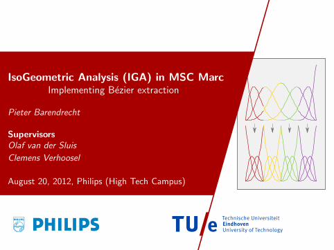
IsoGeometric Analysis (IGA) in MSC MarcImplementing Bezier extraction
Pieter Barendrecht
SupervisorsOlaf van der Sluis
Clemens Verhoosel
August 20, 2012, Philips (High Tech Campus)
The title explained...
IsoGeometric Analysis (IGA): the unification of CAGD and FEA,meaning that the same basis functions will be used for both
MSC Marc : the computational part of the commercial softwarepackage MSC Marc/Mentat
Implementing : writing a practical user element in FORTRAN forMSC Marc
Bezier extraction: the description of a B-Spline curve asconcatenated Bezier curves
Philips & MEFD (Multiscale Engineering Fluid Dynamics)
1
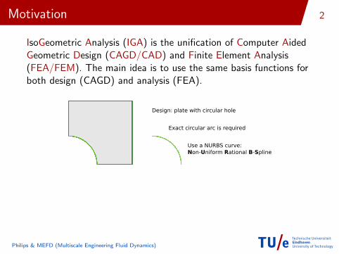
Motivation
IsoGeometric Analysis (IGA) is the unification of Computer AidedGeometric Design (CAGD/CAD) and Finite Element Analysis(FEA/FEM). The main idea is to use the same basis functions forboth design (CAGD) and analysis (FEA).
Design: plate with circular hole
Use a NURBS curve:Non-Uniform Rational B-Spline
Exact circular arc is required
B Relatively new technique. First paper in 2005. Book in 2009.B Therefore not yet available in commercial software packages...B Would it be possible to implement IGA ourselves in such a
software package, e.g. MSC Marc?
Philips & MEFD (Multiscale Engineering Fluid Dynamics)
2

Overview
Computer Aided Geometric Design (CAGD)
Finite Element Analysis (FEA)
Workflow and implementation
Showcase
Conclusions
Philips & MEFD (Multiscale Engineering Fluid Dynamics)
3
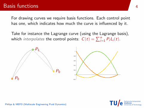
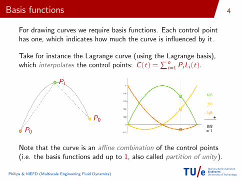
Basis functions
For drawing curves we require basis functions. Each control pointhas one, which indicates how much the curve is influenced by it.
Take for instance the Lagrange curve (using the Lagrange basis),which interpolates the control points: C (t) =
∑ni=1 PiLi (t).
P0
P1
P0
-0.2
0
0.2
0.4
0.6
0.8
1
Note that the curve is an affine combination of the control points(i.e. the basis functions add up to 1, also called partition of unity).
Philips & MEFD (Multiscale Engineering Fluid Dynamics)
4
Basis functions
For drawing curves we require basis functions. Each control pointhas one, which indicates how much the curve is influenced by it.
Take for instance the Lagrange curve (using the Lagrange basis),which interpolates the control points: C (t) =
∑ni=1 PiLi (t).
P0
P1
P0
-0.2
0
0.2
0.4
0.6
0.8
1
6/8
3/8
-1/8
8/8 = 1
+
Note that the curve is an affine combination of the control points(i.e. the basis functions add up to 1, also called partition of unity).
Philips & MEFD (Multiscale Engineering Fluid Dynamics)
4

Bezier curves
The Lagrange curve is not a convex combination of the controlpoints. Numerically spoken, convexity is a nice property to have!
Let’s take a look at different basis functions, the Bernstein basisfunctions. The resulting curve is called a Bezier curve.
P0
P1
P2
0
0.1
0.2
0.3
0.4
0.5
0.6
0.7
0.8
0.9
1
9/16
6/16
1/16
16/16= 1
+
Note that this curve is indeed a convex combination of the controlpoints – but the control points are now only approximated .
Philips & MEFD (Multiscale Engineering Fluid Dynamics)
5
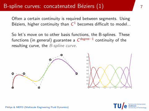
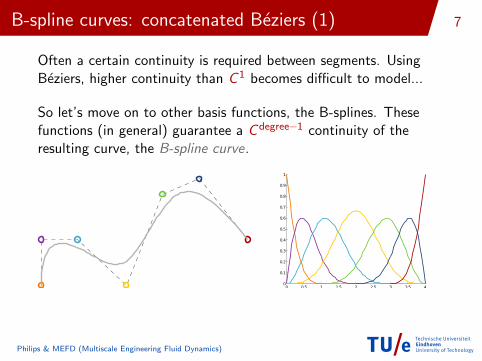
B-spline curves: concatenated Beziers (1)
Often a certain continuity is required between segments. UsingBeziers, higher continuity than C 1 becomes difficult to model...
So let’s move on to other basis functions, the B-splines. Thesefunctions (in general) guarantee a Cdegree−1 continuity of theresulting curve, the B-spline curve.
Philips & MEFD (Multiscale Engineering Fluid Dynamics)
7
B-spline curves: concatenated Beziers (1)
Often a certain continuity is required between segments. UsingBeziers, higher continuity than C 1 becomes difficult to model...
So let’s move on to other basis functions, the B-splines. Thesefunctions (in general) guarantee a Cdegree−1 continuity of theresulting curve, the B-spline curve.
0 0.5 1 1.5 2 2.5 3 3.5 40
0.1
0.2
0.3
0.4
0.5
0.6
0.7
0.8
0.9
1
Philips & MEFD (Multiscale Engineering Fluid Dynamics)
7
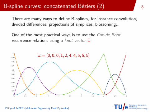
B-spline curves: concatenated Beziers (2)
There are many ways to define B-splines, for instance convolution,divided differences, projections of simplices, blossoming...
One of the most practical ways is to use the Cox-de Boorrecurrence relation, using a knot vector Ξ.
Ξ = [0, 0, 0, 1, 2, 4, 4, 5, 5, 5]
Philips & MEFD (Multiscale Engineering Fluid Dynamics)
8
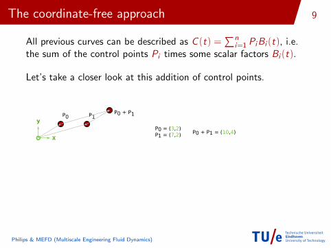
The coordinate-free approach
All previous curves can be described as C (t) =∑n
i=1 PiBi (t), i.e.the sum of the control points Pi times some scalar factors Bi (t).
Let’s take a closer look at this addition of control points.
P0 P1P0 + P1
x
y
P0 = (3,2)P1 = (7,2) P0 + P1 = (10,4)
Philips & MEFD (Multiscale Engineering Fluid Dynamics)
9

The coordinate-free approach
All previous curves can be described as C (t) =∑n
i=1 PiBi (t), i.e.the sum of the control points Pi times some scalar factors Bi (t).
Let’s take a closer look at this addition of control points. Noticethat the position of P0 + P1 is (in a relative sense) dependent onthe position of the origin...!
P0 P1P0 + P1
P0 = (5,2)P1 = (9,2) P0 + P1 = (14,4)
x
y
Philips & MEFD (Multiscale Engineering Fluid Dynamics)
9

The coordinate-free approach
All previous curves can be described as C (t) =∑n
i=1 PiBi (t), i.e.the sum of the control points Pi times some scalar factors Bi (t).
But without an origin, how is it then possible to add points, or tomultiply a point with a scalar value?
x
y P0 P1 No origin anymore! And hence no coordinates.
Only a coordinate system, represented by unit vectors in x and y direction.
This is only possible when using a vector approach, i.e. start withone point P0 and define another point P1 as P0 plus a vector ~v .
This coordinate-free approach leads to the impotant partition ofunity property.
Philips & MEFD (Multiscale Engineering Fluid Dynamics)
9
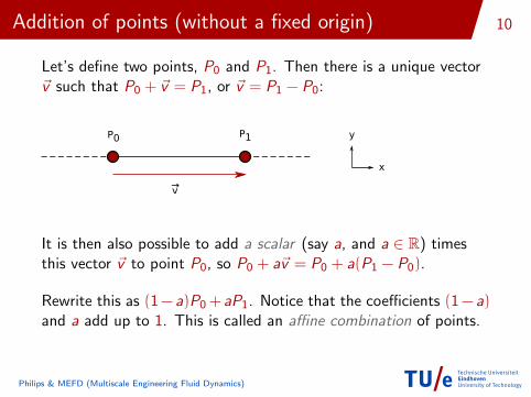
Addition of points (without a fixed origin)
Let’s define two points, P0 and P1. Then there is a unique vector~v such that P0 + ~v = P1, or ~v = P1 − P0:
P0 P1
v→
x
y
It is then also possible to add a scalar (say a, and a ∈ R) timesthis vector ~v to point P0, so P0 + a~v = P0 + a(P1 − P0).
Rewrite this as (1− a)P0+ aP1. Notice that the coefficients (1− a)and a add up to 1. This is called an affine combination of points.
Philips & MEFD (Multiscale Engineering Fluid Dynamics)
10
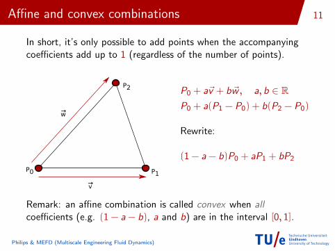
Affine and convex combinations
In short, it’s only possible to add points when the accompanyingcoefficients add up to 1 (regardless of the number of points).
P0
P2
P1
v→
w→
P0 + a~v + b~w , a, b ∈ RP0 + a(P1 − P0) + b(P2 − P0)
Rewrite:
(1 − a − b)P0 + aP1 + bP2
Remark: an affine combination is called convex when allcoefficients (e.g. (1 − a − b), a and b) are in the interval [0, 1].
Philips & MEFD (Multiscale Engineering Fluid Dynamics)
11
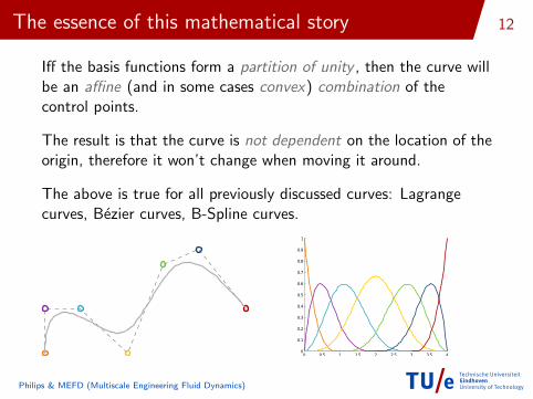
The essence of this mathematical story
Iff the basis functions form a partition of unity , then the curve willbe an affine (and in some cases convex) combination of thecontrol points.
The result is that the curve is not dependent on the location of theorigin, therefore it won’t change when moving it around.
The above is true for all previously discussed curves: Lagrangecurves, Bezier curves, B-Spline curves.
0 0.5 1 1.5 2 2.5 3 3.5 40
0.1
0.2
0.3
0.4
0.5
0.6
0.7
0.8
0.9
1
Philips & MEFD (Multiscale Engineering Fluid Dynamics)
12
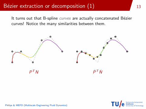
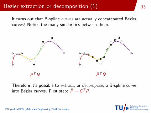
Bezier extraction or decomposition (1)
It turns out that B-spline curves are actually concatenated Beziercurves! Notice the many similarities between them.
PTN PT N
Therefore it’s possible to extract, or decompose, a B-spline curveinto Bezier curves. First step: P = CTP.
Philips & MEFD (Multiscale Engineering Fluid Dynamics)
13
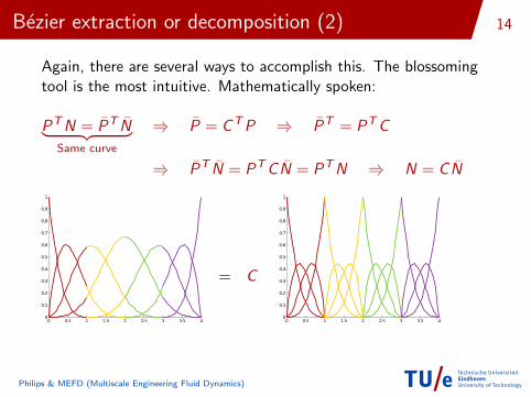
Bezier extraction or decomposition (2)
Again, there are several ways to accomplish this. The blossomingtool is the most intuitive. Mathematically spoken:
PTN = PT N︸ ︷︷ ︸Same curve
⇒ P = CTP ⇒ PT = PTC
⇒ PT N = PTCN = PTN ⇒ N = CN
0 0.5 1 1.5 2 2.5 3 3.5 40
0.1
0.2
0.3
0.4
0.5
0.6
0.7
0.8
0.9
1
= C
0 0.5 1 1.5 2 2.5 3 3.5 40
0.1
0.2
0.3
0.4
0.5
0.6
0.7
0.8
0.9
1
Philips & MEFD (Multiscale Engineering Fluid Dynamics)
14

Basis functions and Finite Element Analysis
FEA is about finding numerical solutions for (partial) differentialequations. Think about heat equations, or elasticity problems.
Exact solution
Piecewise approximation
Elements
This happens in an piecewise-wise fashion. So for each segment, orrather element, there is an associated part of the solution.
Both the elements and parts of the approximated solution arecurves or surfaces. Hence, we require basis functions to describethem.
Philips & MEFD (Multiscale Engineering Fluid Dynamics)
15

The isoparametric concept
A natural approach would be to use the same basis functions forboth the elements and the parts of the (approximated) solution.
In this case, the bi-quadratic Lagrange basis functions. Thisapproach is called the isoparametric concept.
The elements together form the mesh, which approximates themodeled geometry.
Philips & MEFD (Multiscale Engineering Fluid Dynamics)
16

IsoGeometric Analysis (IGA)
CAGD: How should I position my control points, and which basisfunctions should I use to get a satisfying result (i.e. a nice curve)?
FEA: Which elements (basis functions) should I choose, and howshould I position the nodes to get a good result (approximation)?
Two rather similar descriptions, only the terminology/jargon isdifferent. Then why not unite these two?
IGA = CAGD ∪ FEA
Since CAD software uses NURBS (B-Splines) to model geometries,these basis functions will also be used in FEA (the IGA concept).
Philips & MEFD (Multiscale Engineering Fluid Dynamics)
17
IsoGeometric Analysis (IGA)
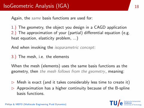
Again, the same basis functions are used for:
1.) The geometry, the object you design in a CAGD application2.) The approximation of your (partial) differential equation (e.g.heat equation, elasticity problem, ...)
And when invoking the isoparametric concept:
3.) The mesh, i.e. the elements
When the mesh (elements) uses the same basis functions as thegeometry, then the mesh follows from the geometry , meaning:
B Mesh is exact (and it takes considerably less time to create it)
B Approximation has a higher continuity because of the B-splinebasis functions.
Philips & MEFD (Multiscale Engineering Fluid Dynamics)
18

Application of Bezier extraction
In classical FEA, every element uses the exact same basis. In caseof IGA, this is not the case anymore. How to solve this?
Do not load individual basis functions for each element, butinstead represent the basis functions as linear combinations of fixed(i.e. for every element the same) basis functions, i.e. the Bernsteinpolynomials: N = CN.
0 0.5 1 1.5 2 2.5 3 3.5 40
0.1
0.2
0.3
0.4
0.5
0.6
0.7
0.8
0.9
1
= C
0 0.5 1 1.5 2 2.5 3 3.5 40
0.1
0.2
0.3
0.4
0.5
0.6
0.7
0.8
0.9
1
Philips & MEFD (Multiscale Engineering Fluid Dynamics)
19

Application of Bezier extraction
In classical FEA, every element uses the exact same basis. In caseof IGA, this is not the case anymore. How to solve this?
Do not load individual basis functions for each element, butinstead represent the basis functions as linear combinations of fixed(i.e. for every element the same) basis functions, i.e. the Bernsteinpolynomials: N = CN.
B Makes it possible to use IGA within existing FEA software
B Only have to implement a new element which uses theBernstein basis
B Element should be able to import the C matrix (in general adifferent one for each element)
Philips & MEFD (Multiscale Engineering Fluid Dynamics)
19

Workflow and implementation
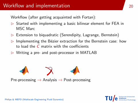
Workflow (after getting acquainted with Fortan):
B Started with implementing a basic bilinear element for FEA inMSC Marc
B Extension to biquadratic (Serendipity, Lagrange, Bernstein)
B Implementing the Bezier extraction for the Bernstein case: howto load the C matrix with the coefficients
B Writing a pre- and post-processor in MATLAB
Pre-processing → Analysis → Post-processing
Philips & MEFD (Multiscale Engineering Fluid Dynamics)
20
Workflow and implementation
Workflow (after getting acquainted with Fortan):
B Started with implementing a basic bilinear element for FEA inMSC Marc
B Extension to biquadratic (Serendipity, Lagrange, Bernstein)
B Implementing the Bezier extraction for the Bernstein case: howto load the C matrix with the coefficients
B Writing a pre- and post-processor in MATLAB
Pre-processing → Analysis → Post-processing
Philips & MEFD (Multiscale Engineering Fluid Dynamics)
20

Pre-processing in MATLAB
Schematic of the test-setup.
Prescribed displacement u→
Philips & MEFD (Multiscale Engineering Fluid Dynamics)
21
Pre-processing in MATLAB
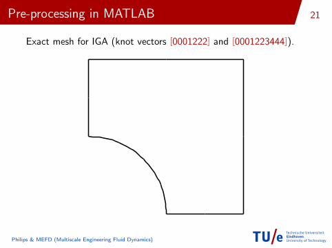
Exact mesh for IGA (knot vectors [0001222] and [0001223444]).
Philips & MEFD (Multiscale Engineering Fluid Dynamics)
21

Pre-processing in MATLAB
Exact mesh for IGA (knot vectors [0001222] and [0001223444]).
Philips & MEFD (Multiscale Engineering Fluid Dynamics)
21

Pre-processing in MATLAB
Exact mesh for IGA (knot vectors [0001222] and [0001223444]).
Philips & MEFD (Multiscale Engineering Fluid Dynamics)
21

Post-processing in MATLAB
Result (the stress field).
Philips & MEFD (Multiscale Engineering Fluid Dynamics)
22
Post-processing in MATLAB
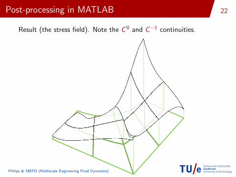
Result (the stress field). Note the C 0 and C−1 continuities.
Philips & MEFD (Multiscale Engineering Fluid Dynamics)
22

Post-processing in MATLAB
Result (the stress field). Note the C 0 and C−1 continuities.
Philips & MEFD (Multiscale Engineering Fluid Dynamics)
22

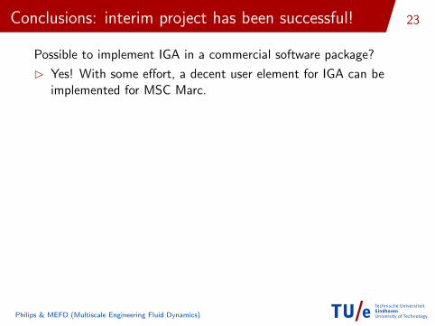
Conclusions: interim project has been successful!
Possible to implement IGA in a commercial software package?
B Yes! With some effort, a decent user element for IGA can beimplemented for MSC Marc.
Nice, but which benefits does IGA provide?
B The mesh really follows from the geometry. The time to createa mesh decreases dramatically!
B The mesh is exact, not an approximation like in classical FEA.
B Solution field (e.g. displacement, stress, temperature) has ahigher continuity, because of the basis functions.
But...
B CAGD is often based on cubic curves, not quadratic ones.Unfortunately, MSC Marc does not provide a cubic ‘ancestor’.
Philips & MEFD (Multiscale Engineering Fluid Dynamics)
23
IsoGeometric Analysis (IGA) in MSC MarcImplementing Bezier extraction
Pieter Barendrecht
SupervisorsOlaf van der Sluis
Clemens Verhoosel
August 20, 2012, Philips (High Tech Campus)
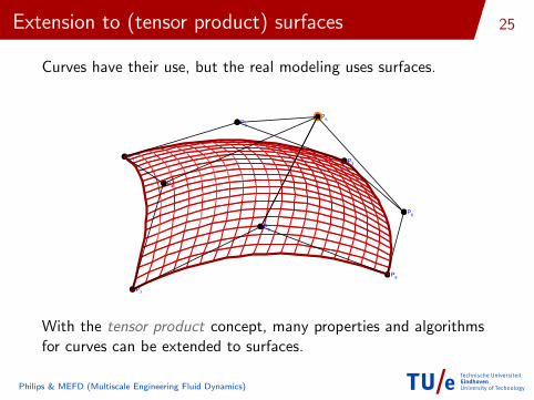
Extension to (tensor product) surfaces
Curves have their use, but the real modeling uses surfaces.
. P1
. P6
. P7
. P8
. P2
. P4
. P9
. P3
. P5
With the tensor product concept, many properties and algorithmsfor curves can be extended to surfaces.
Philips & MEFD (Multiscale Engineering Fluid Dynamics)
25
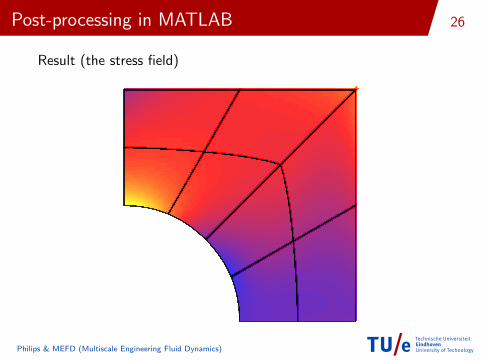
Post-processing in MATLAB
Result (the stress field)
Philips & MEFD (Multiscale Engineering Fluid Dynamics)
26

Post-processing in MATLAB
Result (the stress field)
Philips & MEFD (Multiscale Engineering Fluid Dynamics)
26