ISD 251 QUANTITATIVE METHODS

LECTURE MATERIAL

S. K. AMPONSAH

J. ANNAN

ii

TABLE OF CONTENT

TABLE OF CONTENT ----------------------------------------------------------------------------------- ii

CHAPTER ONE: DIFFERENTIATION AND ITS APPLICATION -------------------------------- 1

CHAPTER TWO: INTEGRATION AND ITS APPLICATION ------------------------------------ 34

CHAPTER THREE: BINOMIAL DISTRIBUTION -------------------------------------------------- 41

CHAPTER FOUR: POISSON DISTRIBUTION ------------------------------------------------------ 55

CHAPTER FIVE: NORMAL DISTRIBUTION------------------------------------------------------- 66

CHAPTER SIX: BUSINESS FORECASTING-------------------------------------------------------- 88

CHAPTER SEVEN: MATRICES AND ITS APPLICATION------------------------------------- 111

1

CHAPTER ONE

DIFFERENTIATION

INTRODUCTION

In this unit, we are going to talk about differentiation, where we shall

concentrate on the standard results, rules, differentiation of exponential

and logarithmic functions, as well as parametric, maxima and minima,

test points, and then the applications of differentiation. The unit will

end with implicit differentiation.

NOTATION

Differentiation is the process of finding the derivative of a function. The

derivative of a function is also called its derived function and also its

derived coefficient.

Rules of Differentiation

1

3

2

5

4

1.0 If then

Examples

( ) If , then

3

( ) If then

5

n

n

y x

dynx

dx

i y x

dyx

dx

ii y x

dyx

dx

2

Note: If auy where a is a constant and u is a function of ,x

then dx

dua

dx

dy

Example

5

4 4

If 7

7(5 ) 35

y x

dyx x

dx

1.1 DIFFERENTIATION OF SUMS AND DIFFERENCES

Here, we differentiate term by term.

Example

If 3 2y x x

23 2dy

xdx

3

1.2 DIFFERENTIATION OF A CONSTANT

0

1

If 5, find .

Solution

5, can be written as 5

(0)(5)

0

dyy

dx

y y x

dyx

dx

Note: Differentiation of a constant is zero

Example

3

2

If 2 1000, .

3 2

dyy x x find

dx

dyx

dx

1.3 Differentiation of Exponential Functions

If

( ) ( )dy then ( )

dx

f x f xy e f x e

Example

1. If

3535 5dx

dy then xx eey

2. If

824824 22

)28(5dx

dyen th5 xxxx exey

4

3. If

dy then 1.

dx

x x xy e e e

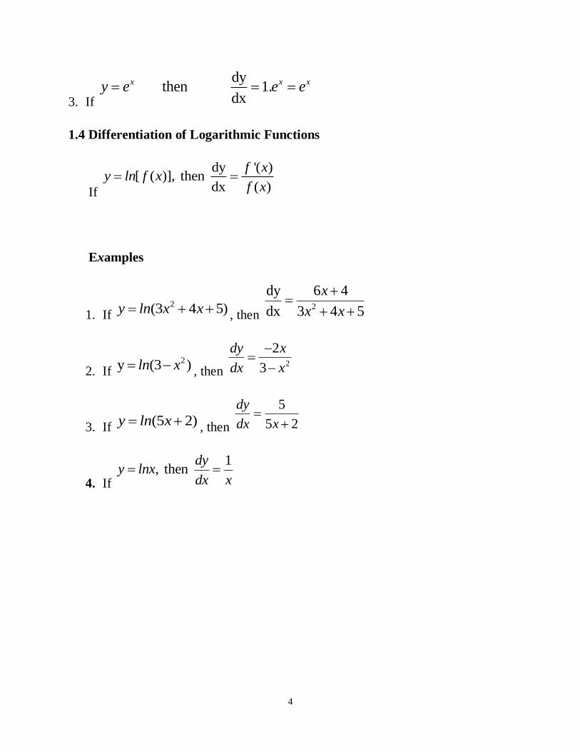
1.4 Differentiation of Logarithmic Functions

If

dy '( )[ ( )], then

dx ( )

f xy ln f x

f x

Examples

1. If 2(3 4 5)y ln x x , then

2

dy 6 4

dx 3 4 5

x

x x

2. If 2y (3 )ln x , then

2

2

3

dy x

dx x

3. If (5 2)y ln x , then

5

5 2

dy

dx x

4. If

1, then

dyy lnx

dx x

5

1.5 DIFFERENTIATION OF PRODUCT OF TWO FUNCTIONS

If y = If and areboth functionsof and thenu v x y uv

dx

dvu

dx

duv

dx

dy..

Examples

(i) If )42)(2( 2 xxy

Let 22 xu and 42 xv

Then 2

dx

dv and 2 x

dx

du

Using dx

dvu

dx

duv

dx

dy..

= 2)2(2)42( 2 xxx

= 4284 22 xxx

= 486 2 xx

6

2 2

2 2

2

2 2

2

( ) ln(3 8 4), .

, ln(3 8 4)

6 82

(3 8 4)

6 8ln(3 8 4)2

(3 8 4)

dyii If y x x x find

dx

Solution

Hereu x and v x x

du dv xx and

dx dx x x

dy du dvv u

dx dx dx

dy xx x x x

dx x x

7

(3 2) 2

(3 2) 2

(3 2)

2

2 (3 2) (3 2)

2

(3 2) 2 (3 2)

2

(3 2)

( ) If ln(3 ), find .

Solution

Here, ln(3 )

23

3

2ln(3 )3 ( )

3

23 ln(3 ) ( )

3

{3ln(3

x

x

x

x x

x x

x

dyiii y e x

dx

u e and v x

du dv xe and

dx dx x

dy du dvv u

dx dx dx

dy xx e e

dx x

xe x e

x

e

2

2

2) ( )}

3

xx

x

1.6 QUOTIENT RULE

If and areboth functionsof and then,u

u v x yv

2v

dx

dvu

dx

duv

dx

dy

8

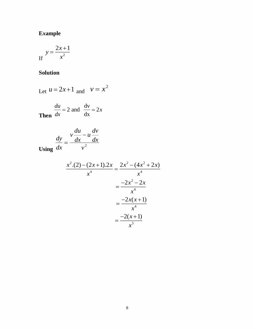
Example

If 2

2 1xy

x

Solution

Let 2 1u x and 2xv

Then

dv2 and 2

dx

dux

dx

Using 2v

dx

dvu

dx

duv

dx

dy

2 2 2

4 4

2

4

4

3

.(2) (2 1).2 2 (4 2 )

2 2

2 ( 1)

2( 1)

x x x x x x

x x

x x

x

x x

x

x

x

9

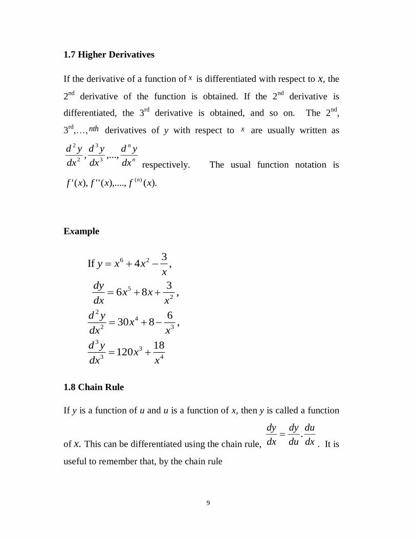
1.7 Higher Derivatives

If the derivative of a function of x is differentiated with respect to x, the

2nd

derivative of the function is obtained. If the 2nd

derivative is

differentiated, the 3rd

derivative is obtained, and so on. The 2nd

,

3rd

,…, nth derivatives of y with respect to x are usually written as

,...,,3

3

2

2

n

n

dx

yd

dx

yd

dx

yd

respectively. The usual function notation is

).(),....,(''),(' )( xfxfxf n

Example

1.8 Chain Rule

If y is a function of u and u is a function of x, then y is called a function

of x. This can be differentiated using the chain rule, dx

du

du

dy

dx

dy.

. It is

useful to remember that, by the chain rule

6 2

5

2

24

2 3

33

3 4

3If 4 ,

3 6 8 ,

630 8 ,

18120

y x xx

dyx x

dx x

d yx

dx x

d yx

dx x

10

2 32( ) ( )

2 , 3 and so ond y dy d y dy

y ydx dx dx dx

.

Example

4 7

4 7

3 6

6 3 3 4 6

Differentiate (3 5) with respect to

Let u 3 5 then y u

so 12 and 7

using . 7 .12 84 (3 5)

y x x

x

du dyx u

dx du

dy dy duu x x x

dx du dx

1.9 IMPLICIT DIFFERENTIATION

If ,242 xxy y is completely defined in terms of x, therefore, y

is called an explicit function of x. Where the relationship between x

and y is more involved, it may not be possible (or desirable) to separate

y completely on the left-hand side, e.g. 2 2xy y

. In such a case

this, y is called an implicit function of x , because a relationship of the

form)(xfy

is implied in the given equation.

It may still be necessary to determine the differential coefficient of y

with respect to x and in fact is not all difficult. All we have to remember

is that y is a function of x , even if it is difficult to see that

2522 yx is an example of an implicit function. Once again, all we

have to remember is that y is a function of x .

So if2522 yx

, let us find dx

dy

.

11

Differentiating with respect to x, we obtain

y

x

dx

dy

xdx

dyy

dx

dyyx

022

Note

To Differentiate an implicit function

a) Differentiate it term by term to give an equation

in x, y and dx

dy

Make dx

dy

the subject of the equation

To obtain the second derivative

a) Differentiate the dx

dy

, equation to obtain an

equation for dx

yd 2

b) Substitute for dx

dy

if necessary.

12

Example 1

If 1056222 yxyx , find and at 2,3 yx

Solution

Differentiate as it stands with respect to x.

06222

dx

dy

dx

dyyx

: .x

dx

dyy 22)62(

62

22

y

x

dx

dy

: . At ( 3, 2 ),

2 2(3)

2(2) 6

2 6 4 = = 2

4 6 2

dy

dx

Then

3

12

2

y

x

dx

d

dx

yd

2)3(

)1()1)(3(

y

dx

dyxy

13

At ( 3,2 )

2 2

2 2

(2 3)( 1) - (1-3) 1 ( 4) = = = 5

(2 3) 1

d y

dx

Example 3

If432 22 yxyx

, find dx

dy

Solution

Differentiating term by term, we have

06)(22 dx

dyyy

dx

dyxx

06222 dx

dyyy

dx

dyxx

022)62( yx

dx

dyyx

yx

dx

dyyx 22)62(

yx

yx

dx

dy

62

)(

14

Example 4

If 83 233 xyyx

, find

Solution

Differentiating term by term, we have

0)1.2.(333 222 ydx

dyyx

dx

dyyx

03633 222 y

dx

dyxy

dx

dyyx

222 33)63( yxdx

dyxyy

xyy

yx

dx

dy

63

33

2

22

Example 5

Given that x2 – 3xy + 2y

2 – 2x = 4, find the value of at the point (1,-

1).

Solution

Differentiating with respect to x, we have

024)(32 dx

dyyy

dx

dyxx

024332 dx

dyyy

dx

dyxx

15

(-3x + 4y) = 2 + 3y – 2x

yx

xy

dx

dy

43

232

at (1,-1) we have

= 7

3

7

3

43

232

Example 6

If 102 22 yx

find (i) (ii)

Solution

i) Differentiating term by term, we have

042

dx

dyyx

x

dx

dyy 24

y

x

y

x

dx

dy

24

2

ii) Differentiating , with respect to x, we have

2)2(

2)()1(2

y

dx

dyxy

16

2)2(

)2

(22

y

y

xy

3

2

2 4

2

)2(

2

y

xy

y

y

xy

EXERCISES

Find (i) if:

i. x3 + y

3 = 3xy

ii. 3x2 + 4xy + y

2 – 6x = 10

iii. 3x2y

2 + 3xy + 4y

2 +10x = 2

iv. 363 322 xxyxyyx

17

1.10 Logarithmic Differentiation

To differentiate a function of the form )(

)(xg

xfy

(a) Take logarithms of the given function

(b) Differentiate the new function as usual

Example 1

If dx

dyfindxy x2

.

Solution

2

2

taking logs on both sides, we have l 2

1 1Differentiating, we have 2 . 2

(2 2 ) (2 2 )

x

x

y x ny xlnx

dyx lnx

y dx x

dyy lnx y x lnx

dx

Example 2

If dx

dyy x find 3

2

2

2 3

1. 2 3

(2 3) 3 (2 )x

lny x ln

dyxln

y dx

dyy xln xlnx

dx

18

1.11 Maxima and Minima

At a point of local maximum, a function has a greater Value than at

points immediately on either side of it. At a point of local minimum, a

function has a smaller Value than at points immediately on either side of

it. Local maxima and minima are also called turning points.

A function may have more than one turning point. The local maxima and

minima are not necessarily the greater or least Values of the function in

the given range.

Local maximum

Local maximum

maximummm

maximum

mm

minimum

m

greatest

mini

mu

m

19

1.12 Tests for Points

A stationary point is a point at which . Local maxima,

minima and horizontal points of inflexion are stationary points. To test

for stationary points,

a) Find and

b) Put and solve the resulting equation to find the x –

coordinate(s) of the point(s)

c) Find at the stationary point(s).

i.) if , the point is local maximum

ii.) if , the point is local minimum

iii.) if , find the sign of )(xf for a value of x just to the left

and just to the right of the point.

Sign to the Left Sign to the Right Types of point

+ - Maximum

- + Minimum

+

-

+

-

}point of inflexion

20

To test general points of inflexion.

a) Find

b) Put and solve the resulting equation to find the

possible x– coordinate(s)

c) Find the sign of for a value of x just to the left and to the

right of the point. If changes sign, the point is a point of

inflexion.

Example 1

Find the stationary points of xxxxf 32

3

1)( 23

and identify their

nature.

Solution

xxxxf 32

3

1)( 23

34)( 2 xxxf

42)( xxf

At stationary points0)( xf

, i.e., 0342 xx ,

0)1)(3( xx

13 xandx

21

When x = 3, 024)3(2)3( f

0)3(3)3(2)3(

3

1)3( 23 f

Therefore (3, 0 ) is a local minimum.

When 024)1(2)1(,1 fx

3

4)1(3)1(2)1(

3

1)1( 23 f

Therefore (1, ) is a local maximum.

Example 2

Find any points of inflexion of32

3

1)( 3 xxxf

.

Solution

32

3

1)( 3 xxxf

xxxf 4)( 2

42)( xxf

At a general point of inflexion 0)( xf , i.e., 2x – 4 = 0 ⇒ x = 2

For x = 2+, 0)( xf i.e. )(xf changes sign

22

For x = 2-, 0)( xf

So x = 2 is a general point of inflexion.

1.13 Applications of Maxima and Minima

Maxima and Minima can be applied to practical problems in which the

maximum or minimum value of a quantity is required. The procedure is

a) Write an expression for the required quantity.

b) Use the given conditions to rewrite it in terms of a single variable.

c) Find the turning point(s) and their type(s). It is often obvious from the

problem itself whether a maximum or minimum has been obtained.

COST, REVENUE AND PROFIT FUNCTIONS

1.14 MARGINAL COST

In business and economics one is often interested in the rate at which

something is taking place. A manufacturer, for example, is not only

interested in the total cost at certain production levels , but also

interested in the rate of change of costs at various production levels.

In economics the word marginal refers to a rate of change; that is, to a

derivative. Thus, if

23

The marginal cost indicates the change in cost for a unit change in

production at a production level of x units if the rate were to remain

constant for the next unit change in production.

Example 1

Suppose the total cost (x) in thousands of cedis for manufacturing x

bags of cement per week is given by

Find

(i) The marginal cost at x

(ii) The marginal cost at x = 1, 2, and 3 levels of production.

Solution

(i)

(ii) ₵6,000 per unit increase in production

(iii) ₵4,000 per unit increase in production

(iv) ₵2,000 per unit increase in production

Notice that, as production goes up, the marginal cost goes down, as we

might expect.

24

Example 2

The total cost per day, for manufacturing

x tones of steel is given by

(i) Find the marginal cost at x

(ii) Find the marginal cost at x = 1, 3, and 4 units level of production.

Marginal Analysis in Business and Economics

Marginal cost, Revenue, and Profit

Applications

Marginal Average cost, Revenue and Profit

Marginal Cost, Revenue, and Profit

One important use of calculus in business and economics is in marginal

analysis. Economists also talk about marginal revenues and marginal

profit.

If x is the number of units of product produced in some time interval

then,

Total cost = C(x)

Marginal cost = C‟(x)

Total revenue = R(x)

Marginal revenue = R‟(x)

Total Profit =

25

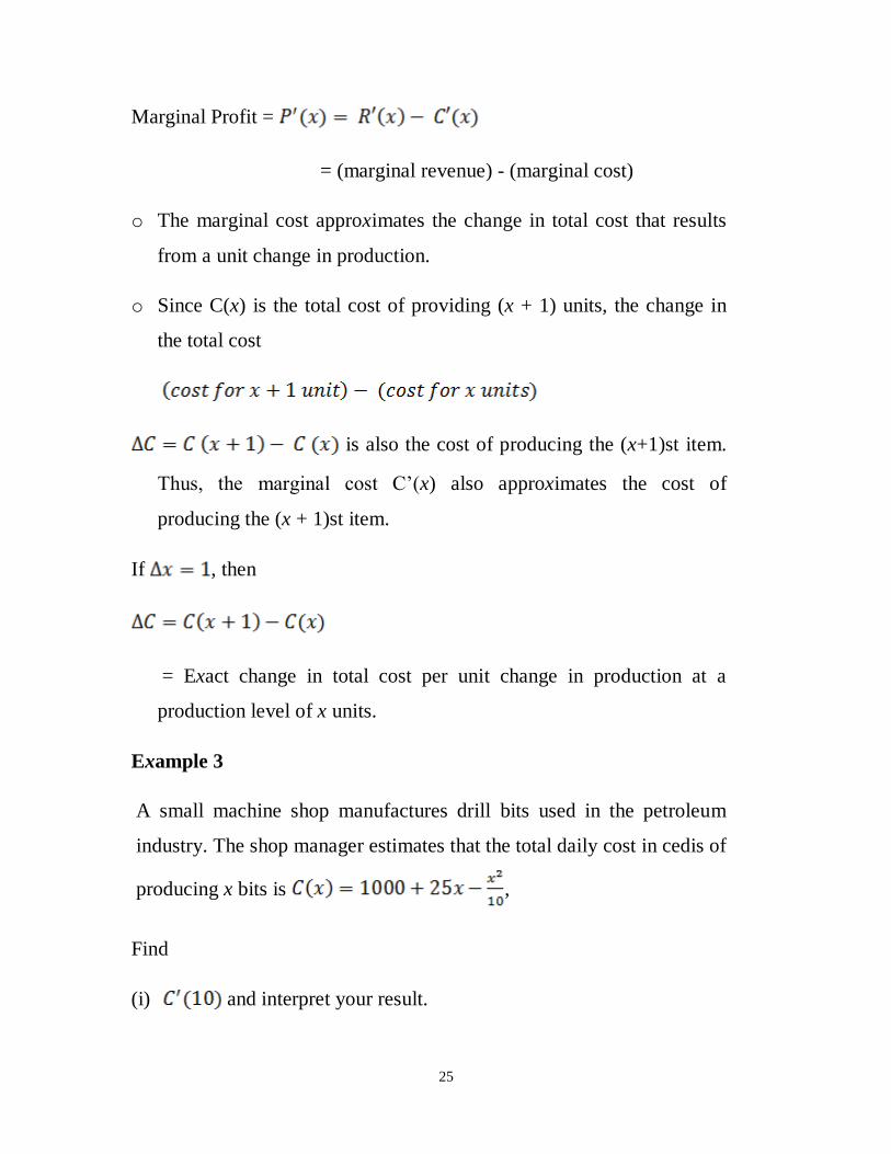
Marginal Profit =

= (marginal revenue) - (marginal cost)

o The marginal cost approximates the change in total cost that results

from a unit change in production.

o Since C(x) is the total cost of providing (x + 1) units, the change in

the total cost

is also the cost of producing the (x+1)st item.

Thus, the marginal cost C‟(x) also approximates the cost of

producing the (x + 1)st item.

If , then

= Exact change in total cost per unit change in production at a

production level of x units.

Example 3

A small machine shop manufactures drill bits used in the petroleum

industry. The shop manager estimates that the total daily cost in cedis of

producing x bits is ,

Find

(i) and interpret your result.

26

(ii) – and interpret your result.

Solution

At production level of 10 bits, a unit increase in production will

increase the total production cost by approximately ₵23. Also the cost

of producing the 11th

bit is approximately ₵23

A STRATEGY FOR SOLVING APPLIED OPTIMIZATION

PROBLEMS

Step 1: Introduce variables and construct a mathematical model of the

form

Maximize (or Minimize) f(x) on the interval I

Step 2: Find the absolute maximum (or minimum) value of f(x) on the

interval I and the value(s) of x where this occurs.

Step 3: Use the solution to the mathematical model to answer the

questions asked in the application.

27

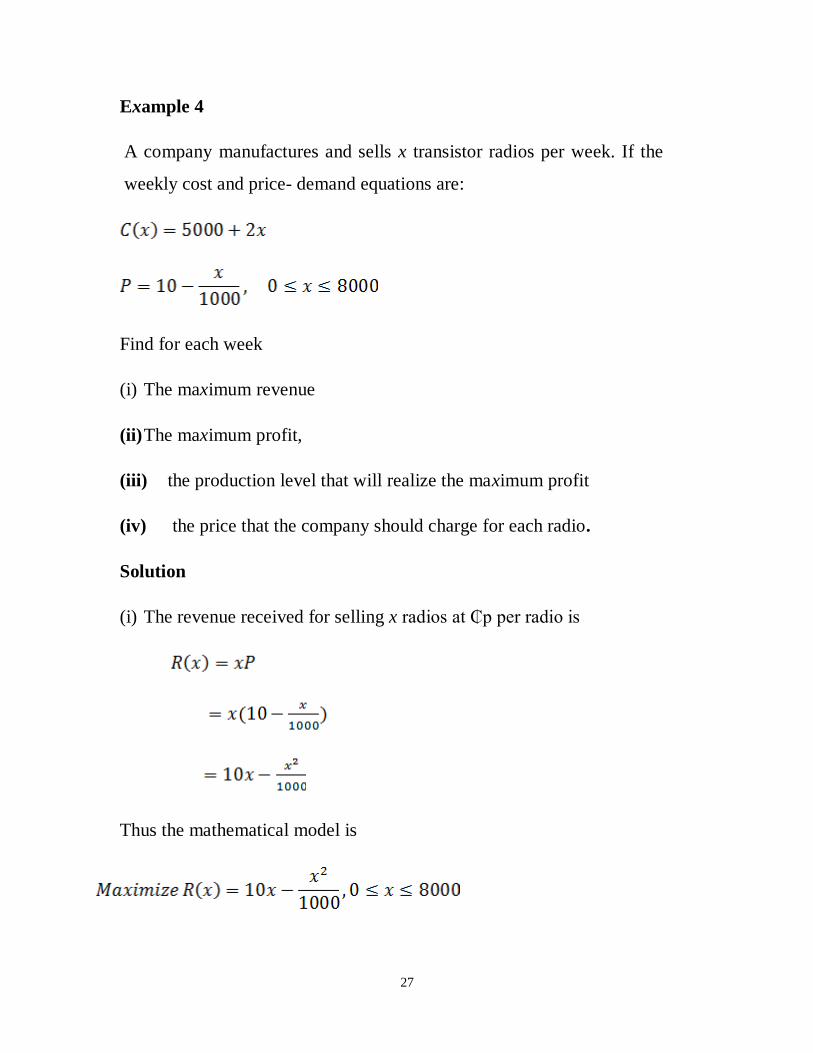
Example 4

A company manufactures and sells x transistor radios per week. If the

weekly cost and price- demand equations are:

Find for each week

(i) The maximum revenue

(ii) The maximum profit,

(iii) the production level that will realize the maximum profit

(iv) the price that the company should charge for each radio.

Solution

(i) The revenue received for selling x radios at ₵p per radio is

Thus the mathematical model is

28

At the critical value,

Use the second derivative test for absolute extrema.

Thus, the maximum revenue is

Profit = Revenue – Cost

The mathematical model is

29

since x = 400 is the only critical value and ,

Now using the price-demand equation with x = 4000, we find

Example 5

Repeat Example (4) for

30

Example 6

In example (4) the government has decided to tax the company ₵2 for

each radio produced. Taking into consideration this additional cost, how

many radios should the company manufacture each in order to

maximize its weekly profit?

What is the maximum weekly profit?

How much should it charge for the radios?

Solution

The tax of ₵2 per unit changes the company‟s cost equation:

C(x) = original cost + tax

= 5000 + 2x + 2x

= 5000 + 4x

The new profit function is

Thus, we must solve the following

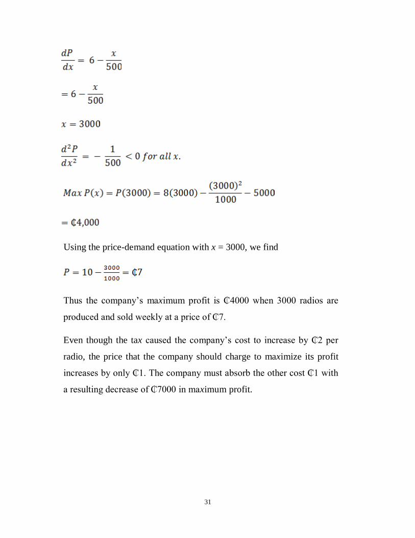
31

Using the price-demand equation with x = 3000, we find

Thus the company‟s maximum profit is ₵4000 when 3000 radios are

produced and sold weekly at a price of ₵7.

Even though the tax caused the company‟s cost to increase by ₵2 per

radio, the price that the company should charge to maximize its profit

increases by only ₵1. The company must absorb the other cost ₵1 with

a resulting decrease of ₵7000 in maximum profit.

32

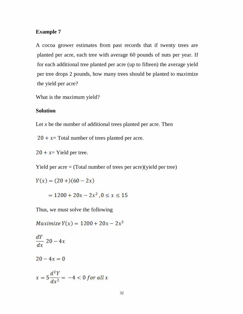
Example 7

A cocoa grower estimates from past records that if twenty trees are

planted per acre, each tree with average 60 pounds of nuts per year. If

for each additional tree planted per acre (up to fifteen) the average yield

per tree drops 2 pounds, how many trees should be planted to maximize

the yield per acre?

What is the maximum yield?

Solution

Let x be the number of additional trees planted per acre. Then

= Total number of trees planted per acre.

= Yield per tree.

Yield per acre = (Total number of trees per acre)(yield per tree)

Thus, we must solve the following

33

Hence pounds per acre. Thus, a maximum

yield od 1250 pounds of nuts per acre is realized of twenty-five trees

are planted per acre.

EXERCISE

Repeat Example, starting with thirty trees per acre and

a reduction of 1 pound per tree for each additional

tree planted.

34

CHAPTER TWO

INTEGRATION

THE INDEFINITE INTEGRAL

In our study of the theory of the firm, we have worked with total cost,

total revenue and the profit functions and have found their marginal

functions. In practice, it is often easier for a company to measure

marginal cost, revenue, and

profit.

If the marginal revenue of a firm is given by 300 0.5 , where is the number

of units sold

MR Q Q

If we want to use this function to find the total revenue function, we need

to find R(Q) from the

1

fact that . In this situation, we need to reverse the process of differentiation.

This process is called integration. By integration we can write ( ) (300 0.5 )

In general [I1

nn

dRMR

dQ

R Q Q dQ

xx dx K

n

ncrease the exponent of by 1 and divide by the new power]

and is an arbitrary constant.

x

K

Example 1

Evaluate 3dx

Solution

35

0 0 13 3 3

3

dx x dx x K

x K

Example 2

Evaluate

58x dx

Solution

5 5 186

643

8x dx x K

x K

Example 3

Evaluate 2(3 2 1)x x dx

Solution

2 2 1 1 1 0 13 2 13 2 1

3 2

(3 2 1)x x dx x x x K

x x x K

Example 4

The marginal revenue in dollars per unit for a motherboard

is 300 0.2MR x , where x represent the quantity sold. Find the

(i) revenue function;

(ii) total revenue from the sale of 1000 motherboards.

Solution

36

(i) We know that the marginal revenue can be found by differentiating

the total revenue function. That is, '( ) 300 0.2R x x

Thus integrating the marginal revenue function gives the total revenue

function

20.22

2

2

2

( ) (300 0.2 )

300

300 0.1

But there is no revenue, when no units are sold, thus 0, when 0

0 300(0) 0.1(0)

0

The total revenue function is: ( ) 300 0.1

(ii) The total reven

x

R x x dx

x K

x x K

R x

K

K

R x x x

2

ue from the sale of 1000 motherboards is

(1000) 300(1000) 0.1(1000)

300,000 100,000

$200,000

R

Example 5

Suppose the marginal cost function for a month for a certain product is

3 50MC Q , where Q is the number of units and the cost in cedis. If

the fixed costs related to the product amount to GH¢100 per month,

find the total cost function for the month.

Solution

37

1 1 0 13 12 1

232

232

232

The total cost function is: ( ) (3 50)

50

50

But when 0, 100

100 (0) 50(0)

100

( ) 50 100

C Q Q dQ

Q Q K

Q Q K

Q FC

K

K

C Q Q Q

Example 6

A firms marginal cost function for a product is 2 50MC Q , its

marginal revenue function is 200 4MR Q and that the cost of

production and sale of 10 units is GH¢700. Find the

(i) optimal level of production;

(ii) profit function

(iii) profit or loss at the optimal level.

Solution

(i) Profit is maximized when

200 4 2 50

200 50 2 4

150 6

25

The level of production that will maximize profit is 25 units

MR MC

Q Q

Q Q

Q

Q

38

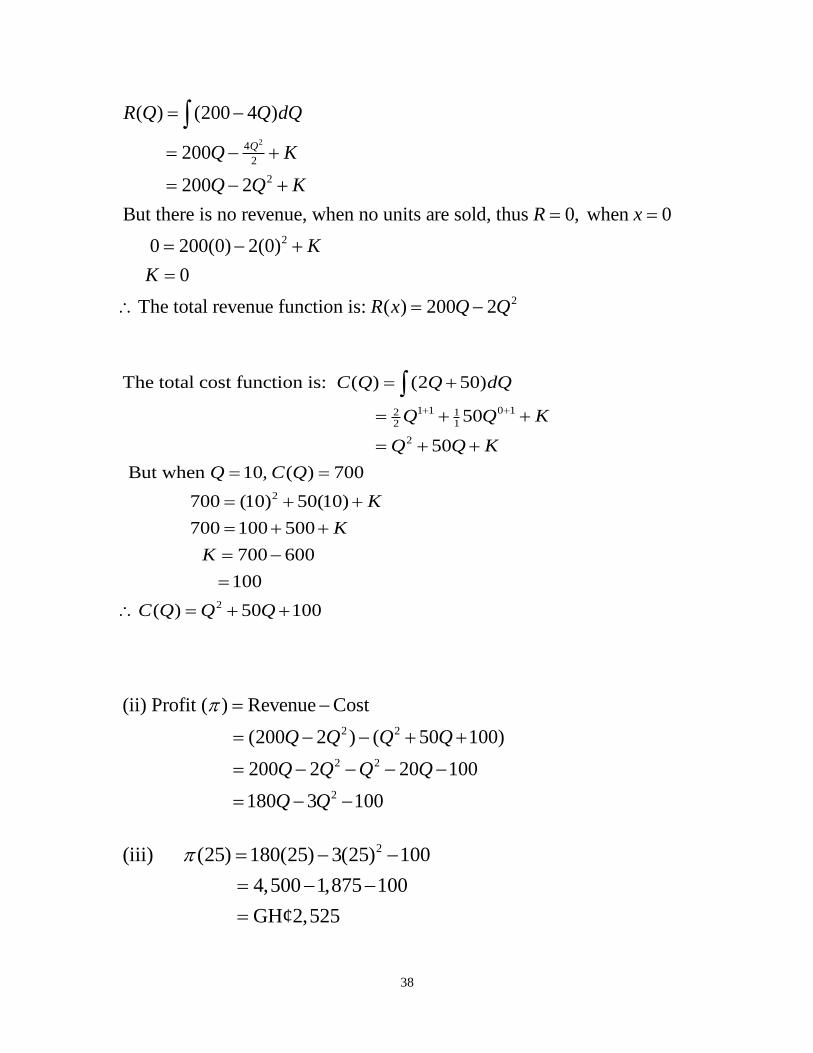
24

2

2

2

2

( ) (200 4 )

200

200 2

But there is no revenue, when no units are sold, thus 0, when 0

0 200(0) 2(0)

0

The total revenue function is: ( ) 200 2

Q

R Q Q dQ

Q K

Q Q K

R x

K

K

R x Q Q

1 1 0 12 12 1

2

2

2

The total cost function is: ( ) (2 50)

50

50

But when 10, ( ) 700

700 (10) 50(10)

700 100 500

700 600

100

( ) 50 100

C Q Q dQ

Q Q K

Q Q K

Q C Q

K

K

K

C Q Q Q

2 2

2 2

2

(ii) Profit ( ) Revenue Cost

(200 2 ) ( 50 100)

200 2 20 100

180 3 100

Q Q Q Q

Q Q Q Q

Q Q

2(iii) (25) 180(25) 3(25) 100

4,500 1,875 100

GH¢2,525

39

Exercise

1. Evaluate each of the following

2

2

3 2

(i) (3 2)

(ii) (3 5)

(iii) (6 2 4)

(iv) (12 15 8 6)

x dx

Q dQ

x x dx

Q Q Q dQ

2. The marginal revenue (in dollars per unit) for a month for a

commodity is 0.05 25MR Q , find the total revenue function

3. If the marginal revenue (in cedis per unit) for a month is given

by 450 0.3MR Q , what is the total revenue from the production

and sale of 50 units

4. If the monthly marginal cost for a product is 2 100MC x , with

fixed cost amounting to $200, find the total cost function for the

month.

5. If the marginal cost for a product is 4 2MC x and the production

of 10 units results in a total cost of $300, find the

(i) total cost function

(ii) total cost of producing 200 units of the product.

40

6. A certain firm‟s marginal cost for a product is 6 60MC Q , its

marginal revenue is 180 2MR Q , and the total cost of producing 10

items is GH¢1000. Find the

(i) optimal level of production;

(ii) profit function;

(iii) profit or loss at the optimal level of production.

41

CHAPTER THREE

BINOMIAL DISTRIBUTION

INTRODUCTION

Some experiments can result in only two possible outcomes. For

example the answer to a question may be yes or no. If a coin is tossed,

we may obtain either a Head or a Tail. A person selected at random

may be male or female; a student may be wearing glasses or not

wearing glasses. Thus the result of a trial is one of the two

complementary results.

Suppose that the experiment is performed a fixed number of times, n,

say, and that the probability, p, of obtaining one particular outcome (i.e.

what we are interested in) called the probability of success, remains the

same from trial to trial. The probability, of the other outcome

(i.e. what we are not interested in) is called probability of failure. In this

case, we observe that . The repeated trials are independent

and that the total number of successes is the variable of interest.

An experiment with these characteristics is said to fit the Binomial

model and the

outcome is a binomial variable.

DEFINITION

Let E be an event and p be the probability that E will happen in any

single trial. The number p is called the probability of a success. Then q

42

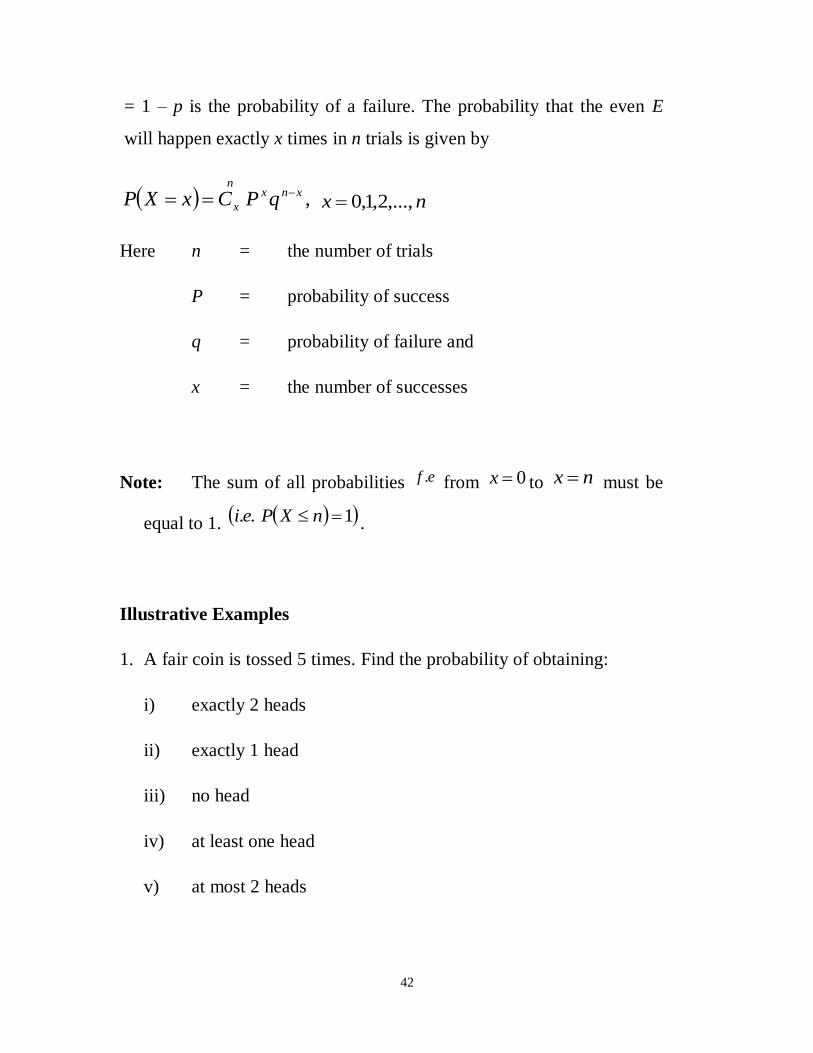
= 1 – p is the probability of a failure. The probability that the even E

will happen exactly x times in n trials is given by

,xnxn

x qPCxXP nx ,...,2,1,0

Here n = the number of trials

P = probability of success

q = probability of failure and

x = the number of successes

Note: The sum of all probabilities ef . from 0x to nx must be

equal to 1. 1.. nXPei .

Illustrative Examples

1. A fair coin is tossed 5 times. Find the probability of obtaining:

i) exactly 2 heads

ii) exactly 1 head

iii) no head

iv) at least one head

v) at most 2 heads

43

Solution

Here PheadP

2

1

qtailP

2

1

n = 5

Now we can see that from (i) – (v), we are interested in the number of

heads and so the probability of head becomes the probability of success.

i) headsexactlyP 2 = 2XP

=

325

22

1

2

1

C

= 8

1

4

110

= 32

10

= 16

5

ii) headexactlyP 1 = 1xP =

415

12

1

2

1

C

= 16

1

2

15

= 32

5

iii) headnoP = 0xP =

505

02

1

2

1

C

=

5

2

111

= 32

1

iv) headoneleastatP = 1xP =

54321 xPxPxPxPxP

0 1 2 3 4 5 1 2 3 4 5

44

This can be evaluated as 1xP = 01 xP = 32

11

= 32

31

v) headsmostatP 2 = 2xP = 210 xPxPxP

= 32

10

32

5

32

1

= 32

16

= 2

1

Example 2

It is known 20% of parts produced by a certain machine are defective. If

six parts produced by the machine are selected at randomly from a

day‟s rum, find the probability that:

i) all six of the parts are defective

ii) none of them is defective

iii) exactly 2 of them are defective

Solution

n = 6

defectiveP = 100

20

= 0.2 P

defectivenonP = 1 – 0.2 = 0.8 q

Here from (i) to (iii) we are interested in defective parts and so

defectiveP = successofyprobabilitP .

i) defectiveareallP = 6xP = 06

6

6

8.02.0C

45

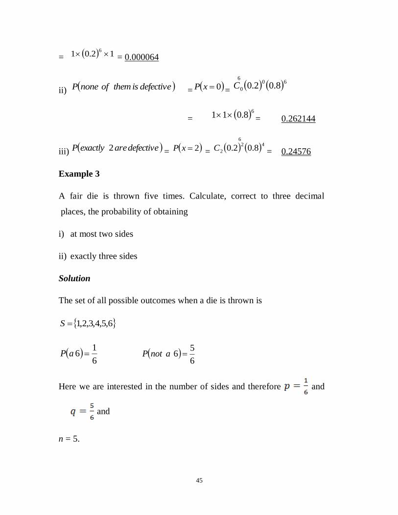
= 12.016 = 0.000064

ii) defectiveisthemofnoneP = 0xP = 60

6

0 8.02.0C

= 68.011 = 0.262144

iii) defectiveareexactlyP 2 = 2xP = 6

42

2 8.02.0C = 0.24576

Example 3

A fair die is thrown five times. Calculate, correct to three decimal

places, the probability of obtaining

i) at most two sides

ii) exactly three sides

Solution

The set of all possible outcomes when a die is thrown is

6,5,4,3,2,1S

6

16 aP

6

56 anotP

Here we are interested in the number of sides and therefore and

and

n = 5.

46

i) sixestwomostatP = 210 xPxPxP

=

325

2

915

1

505

0 6

5

6

1

6

5

6

1

6

5

6

1

CCC

= 0.4019 + 0.4019 + 0.1608

= 0.9646

= 0.965 to 3 decimal places

ii) sixesthreeexactlyP = 3xP

=

235

3 6

5

6

1

C

= 0.03215

= 0.032 to 3 decimal places

Example 4

A machine that manufactures engine parts has an average probability of

0.2 of breaking down. If a factory has 10 of these machines, what is the

probability that at least 8 will be in good working order.

Solution

downbreakingP = 0.2 q

orderworkinggoodP = 1 – 0.2 = 0.8 P

n = 10

47

We are required to find the probability of being in good working order

and therefore p=0.8 and q=0.2

8leastatP = 1098 xPxPxP

= 010

10

10

2910

9

2810

82.08.02.08.02.08.0 CCC

= 0.3020 + 0.2684 + 0.1074

= 0.6778

Example 5

A box contains 12 balls, three of which are defective. If a random

sample of 5 is drawn from the box one after the other with replacement,

what is the probability that

(a) exactly one is defective?

(b) at most one is defective?

Solution

defectiveP = P 25.0

12

3

defectivenonP = 1 – 25 = q75.0

n = 5

(a) defectiveisoneexactlyP = 1xP

48

= 41

5

175.025.0C

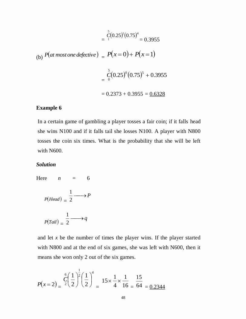
= 0.3955

(b) defectiveonemostatP = 10 xPxP

= 3955.075.025.0

505

0C

= 0.2373 + 0.3955 = 0.6328

Example 6

In a certain game of gambling a player tosses a fair coin; if it falls head

she wins N100 and if it falls tail she losses N100. A player with N800

tosses the coin six times. What is the probability that she will be left

with N600.

Solution

Here n = 6

HeadP = P

2

1

TailP = q

2

1

and let x be the number of times the player wins. If the player started

with N800 and at the end of six games, she was left with N600, then it

means she won only 2 out of the six games.

2xP =

42

1

6

2 2

1

2

1

C

= 16

1

4

115

= 64

15

= 0.2344

49

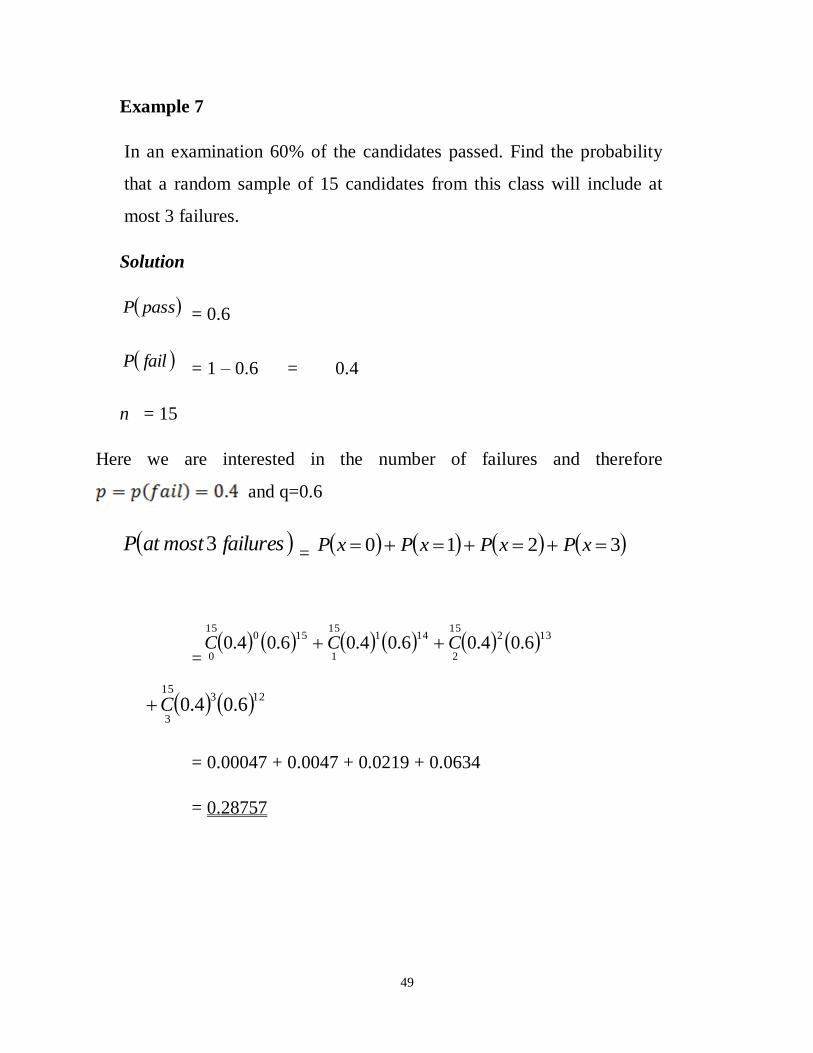
Example 7

In an examination 60% of the candidates passed. Find the probability

that a random sample of 15 candidates from this class will include at

most 3 failures.

Solution

passP = 0.6

failP = 1 – 0.6 = 0.4

n = 15

Here we are interested in the number of failures and therefore

and q=0.6

failuresmostatP 3 = 3210 xPxPxPxP

= 132

15

2

14115

1

15015

06.04.06.04.06.04.0 CCC

12315

36.04.0C

= 0.00047 + 0.0047 + 0.0219 + 0.0634

= 0.28757

50

Example 8

A farmer produces seeds in packets for sale. The probability that a seed

selected at random will grow is 0.80. If 6 of these seeds are sown, what

is the probability that

i) less than two will grow?

ii) less than two will not grow?

iii) exactly half the seeds will grow?

Solution

Number of seeds, n = 6

growP = 0.8

grownotP = 0.2

i) Here 8.0P , ,2.0q n = 6

P(less than two will grow) = P (X=0) + P(X=1)

= 51

6

1

606

02.08.02.08.0 CC

= 0.0016

ii) P(less than 2 will not grow)

Here we are interested in not grow

51

Hence p=0.2 and q=0.8

2xP

= 10 xPxP

= 51

6

1

606

08.02.08.02.0 CC

= 0.65536

iii) P(exactly half of the seeds will grow) 36

2

1

Thus 3xP

where p=0.8, q=0.2 and n=6

3xP = 33

6

32.08.0C

= 0.08192

Example 9

A question paper contains 8 multiple-choice questions, each with 4

answers of which only one is the correct answer. If a student guesses at

the answers, find the probability that he gets

i) no correct answer

ii) exactly 3 correct answers

iii) at most 3 correct answers

Solution

correctlyanswersheP =

P4

1

52

wronglyanswersheP = q

4

3

i) 0xP =

808

0 4

3

4

1

C

= 0.1001129

ii) 3xP =

538

3 4

3

4

1

C

= 0.2076

iii) 3xP = 3210 xPxPxPxP

=

538

3

628

2

718

1 4

3

4

1

4

3

4

1

4

3

4

11001.0

CCC

= 0.10011 + 0.26698 + 0.31146 + 0.20764

= 0.88619

Example 10

A large consignment of manufactured articles is accepted if either of the

following conditions is satisfied:

i) A random sample of 10 articles contains no defective articles

ii) A random sample of 10 contains one defective article and a second

random sample of 10 is then drawn which contains no defective

articles.

53

Otherwise the consignment is rejected. If 5% of the articles in a given

consignment are defective, what is the probability that the consignment

is accepted?

Solution

defectiveP =

p 05.0100

5

defectivenonP = q95.0

n = 10

Condition (i)

0xP =

10010

095.05.0C

0.5987

Condition (ii)

01 xPxP

= 5987.095.005.0

9110

1C

= 0.3151 x 0.5987 = 0.1887

Therefore the probability of accepting the consignment = (i) or (ii)

= 0.5987 + 0.1887

= 0.7874

54

Exercises

1. A fair coin is tossed six times. Find the probability of obtaining at

least four heads.

2. 30% of pupils in a school travel to school by bus. From a sample of 8

pupils chosen at random, find the probability that

(a) only three travel by bus

(b) less than half travel by bus

3. A fair die is thrown 7 times. Find the probability of throwing more

than 4 sizes.

4. A fair coin is tossed 12 times. Find the probability of obtaining 7

tails.

5. The probability of an arrow hitting a target is 0.9. Find the

probability of at least 3 arrows hitting the target if 5 arrows are shot.

6. If there are 10 traffic lights along a certain road, find the probability

of getting 2 red lights if the probability of a red light is 5

2

.

55

CHAPTER FOUR

POISSON DISTRIBUTION

INTRODUCTION

Sometimes, one may be interested in occurrences in a specified time

period, length, area or volume. For example, at certain times of the year

there are virtually no accidents whilst more traffic accidents are

recorded on occasions like Easter, Christmas, National holidays,

Ramadan festivals. One may therefore be interested in finding the

probability of a number of traffic accidents, which would occur, in a

festive period or a fraction of a festive period. It is also known that at

certain times of the week one finds a large number of airplanes at

Kotoka International Airport whilst at other times, no planes are found

at the airport.

It is known that at certain times, e.g. some few days after pay day, one

finds a large number of customers in a queue at the cashier‟s counter in

banks, whilst at other times, the banks are virtually empty, and therefore

no customer at the cashier‟s counter.

Other examples of such variables are; the number of mistakes on a

paper of a book, number of radio-active elements detected by a Geiger-

counter; number of ships arriving at an harbour in a particular time

period; number of flaws in a textile (cloth); number of fire outbreaks in

a given period of time; the number of breakdowns of machines per year;

number of telephone calls on Monday between 8am and 9am.

These events have certain characteristics.

56

i. The events occur at random in continuous space or time.

ii. The events occur singly, and the probability of two or more events

occurring at the same time is zero.

iii. The events occur uniformly. Thus the expected number of events in a

given interval is proportional to the size of the interval.

iv. The events are independent.

v. The variable is the NUMBER of events that occur in an interval of a

given size.

DEFINITION:

The number x of successes in a Poisson experiment is called a Poisson

random variable. The probability distribution of the Poisson variable, x

is

( , )

!

xeP x

x

where x = 0,1,2,3… and is the average number of successes in the

given time interval or length, or space or volume. The Poisson

distribution is completely defined by its mean, =np. It is an

approximation to the Binomial when the number of trials is large (n

>30) but np <5.

The mean,, depends on the size of the stated unit. It changes

proportionally whenever the stated unit is changed.

57

The Poisson distribution is given by

0, 1, 2, …

2 31...

0! 1! 2! 3!e

=

= 1

Therefore s a probability distribution.

The expected value of the Poisson distribution = .

The variance of the Poisson distribution is also . This is the only

distribution whose mean and variance are the same.

Example 1

58

Given that X is a Poisson variable with mean, = 2.

Calculate the following probabilities:

(i) 0XP

(ii) 2XP

(iii) 1XP

(iv) 2XP

Solution

(i)

2 022

0 0.13530!

eX eP

(ii)

2 222

2 2 0.27062!

eX eP

(iii) 1 1 ( 1)X P xP

2 1

0 1

21 0.1353

1!

1 0.1353 0.2706

0.5941

1 X P X

e

P

(iv) 2 1 ( 2)X P xP

0 1 2

1 0.1353 0.2706 0.2706

0.3235

1 X P X P XP

59

Example 2

The probability that an insurance company must pay a particular

medical claim for a policy is 0.001. If the company has 1000 of such

policyholders, what is the probability that the insurance company will

have to pay at least 2 claims?

Solution

This is a typical Binomial variable. However with ( )

and ( ) we use the Poisson approximation.

Thus =

=

= 1

1 0 1 1

1

2 1 1

1 0 1

1 11

0! 1!

1 2

0.2642

X P X

P X P X

e e

e

P

60

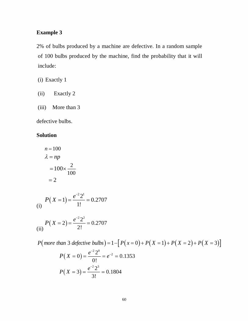
Example 3

2% of bulbs produced by a machine are defective. In a random sample

of 100 bulbs produced by the machine, find the probability that it will

include:

(i) Exactly 1

(ii) Exactly 2

(iii) More than 3

defective bulbs.

Solution

100

2

100100

2

n

np

(i)

2 121 0.2707

1!

eXP

(ii)

2 222 0.2707

2!

eXP

3 1 0 1 2 3P more than defective bulbs P x P X P X P X

2 02

2 3

20 0.1353

0!

23 0.1804

3!

eX e

eP X

P

61

Hence the required probability 0.1353 0.2707 0.2707 0.1804

0.8571

Example 5

Suppose there is an average of 10 fire outbreaks in 20 days of a certain

month. What is the expected number of fire outbreaks in 10 days of that

month?

Solution

In 20 days, mean number = 10

Therefore, in 10 days, mean number =

Thus having the stated number also halves the expected number.

Similarly, doubling the expected number unit also doubles the expected

number of occurrences for the new stated unit.

Example 4

The expected number of telephone calls is 6 per minute.

What is the probability of getting

(a) 4 calls in the next two minutes?

(b) 2 calls in the next thirty seconds?

62

Solution

(a) New mean,

2

16 12 / 2mincalls s

12 4

4!

12

4!

0.0053

xeX

x

e

P

(b) The new mean,

30

606 3 /30mincalls s

Therefore

3 232 0.2240

2!

eXP

Example 5

Suppose there is an average of 10 fire outbreaks in 20 days of a certain

month. What is the expected number of fire outbreaks in 10 days of that

month?

Solution

In 20 days, mean number = 10

Therefore, in 10 days, mean number =

63

Thus having the stated number also halves the expected number.

Similarly, doubling the expected number unit also doubles the expected

number of occurrences for the new stated unit.

Example 6

A typist averages two errors per page of a report. Assuming that the

number of errors is a Poisson variable, calculate the probability that

(i) Exactly two errors will be found on a given page of the report.

(ii) At most three errors will be found on any two pages of the report.

Solution:

(i) The stated units are the same

Thus = 2/page

P(x = 2) =

= 2e-2

(ii) The stated units have changed.

New mean, = errors/2 pages

P(x 3) = P(x = 0) + P(x = 1) + P(x = 2) + P(x = 3)

=

64

= e-4

(1 + 4 + 8 + 10.667)

= 23.667e-4

= (23.667) (0.0183)

= 0.4331

Exercises:

1. (a) The fire department in a city can put out a fire in 1 hour, and the

average is 2.4.

i. What is the probability that no alarms are received for 1 hour?

ii. What is the probability that no alarms are received in 2 hours?

iii. What is the most probable number of alarms in an hour?

2. If a keyboard operator averages two errors per page of newsprint,

and if these errors follow Poisson distribution, what is the

probability that

i. Exactly four errors will be found on a given page?

ii. At least two errors will be found?

3. The number of misprints in a book is Poisson distributed with an

average of 5 in 10 pages. What is the probability of getting at most 1

error on a page of a book? If 5 pages of the book are selected at

random, what is the probability of getting at least 2 pages with at

most1 error on a page?

65

4. A car hire company finds that over a period, the expected demand for

cars is 2 per working day. The cars are hired for one-day return

journeys only.

Assuming that the demand for cars is a Poisson variable,

i. Calculate the probability that there is no demand for cars on any

working day.

ii. If the company has two cars, what is the probability that the company

cannot cope with demand?

iii. The company makes a profit of ¢15,000.00 per day when a car is out

for hire and loses ¢10,000.00 each day a car is not used. Would it be

profitable for the company to buy another car if the average demand

for cars remained at 2 per day?

5. The number of misprints in a book is Poisson distributed with an

average of 5 in 10 pages. What is the probability of getting at most 1

error on a page of a book?

If 10 pages of the book are selected at random, what is the probability

of getting at least 2 pages with at most 1 error?

66

CHAPTER FIVE

NORMAL DISTRIBUTION

INTRODUCTION

This is one of the most widely used continuous probability

distributions. Like all continuous distributions, probabilities of

occurrence of continuous variables are computed as a ratio of length of

a section to total length, volume of a section to total volume or area to

total area. For a continuous variable, the probability at any point is

ZERO i.e. ( ) 0P X c

All normal distributions have the same “bell –shape”. They are

symmetrical about the mean. The scores range from negative infinity

through zero to plus infinity ( )X

There are an infinite number of normal distributions. Each normal

distribution is completely defined if the MEAN and STANDARD

DEVIATION are specified.

It has the probability function

2( )

21

( )2

x

f x e

One special normal distribution is of special interest. This is the UNIT

NORMAL

67

UNIT NORMAL DISTRIBUTION

The NORMAL DISTRIBUTION has a mean, =0 and a standard

deviation, = 1. The scores range between all positive and negative

Numbers i.e. ( )Z .

The scores are usually referred to as STANDARD SCORES. The mean,

median and mode coincide at 0. i.e. It is symmetric about = 0. The total

area under the curve =1. It has the probability function

2

21

( )2

x

f z e dx

= Area under the curve (since the total area

under the curve = 1)

The total probability of a score, a , from – and including that Z

value

(a) = .P Z a

has been computed and presented in the form of a

table often called the Normal Distribution Table.

Example 1

= 0.9772; =0.9332

You must have realized that although the range of standard scores is

from negative infinity to positive infinity, the values of (a) =

68

P Z a have been provided for only positive scores. There is an

easy method of evaluating P Z a

say.

The unit normal distribution is symmetrical about the mean =0. Thus

area in the interval ,0a

is the same as the area in the interval 0,a

.

Thus P (Z < - a ) = P (Z> a ) =1-P (Z< a ) (because the total area under the

curve = 1)

This gives a simple relationship between P (Z< a ) and P (Z < -a) = 1- P

(Z <a).

i.e. (-a) =1 - (a)

-a

NOTE

P (Z < - 2) = 1 - P (Z < 2) i.e. (-2) =1 - (2)

P (Z < -1.5)= 1- P (Z < 1.5) i.e. (-1.5) =1 - (1.5)

69

Example 2

Find i) P (Z <- 0.25); ii) P (Z- < 0.05); iii) P (Z < -0.5)

Solution

i) P (Z <- 0.25) = 1 P (Z< 0.25)

= 1 (0.25)

= 1 0.5987

= 0.4013

ii) P (Z-<0.05) = 1 P (Z< 0.05)

= 1 (0.05)

= 1 0.5199

= 0.4801

iii) P (Z<-0.5) = 1 P (Z< 0.5)

= 1 (0.5)

= 1 0.6915

= 0.3085

Note that the probability of a negative value on the UNIT NORMAL

SCALE is less than 0.5

70

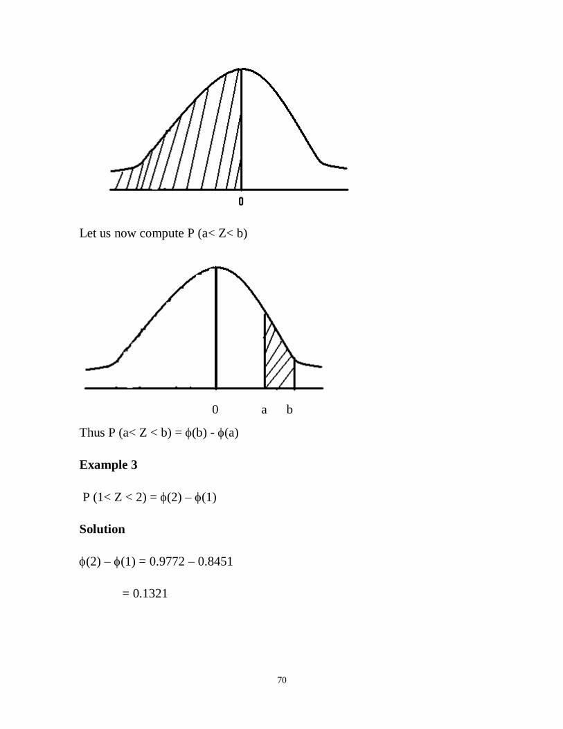
Let us now compute P (a< Z< b)

0 a b

Thus P (a< Z < b) = (b) - (a)

Example 3

P (1< Z < 2) = (2) – (1)

Solution

(2) – (1) = 0.9772 – 0.8451

= 0.1321

71

Example 4

P (- 1.96 < Z < 1.96.) = (1.96) – (-1.96)

= (1.96) – [1-(1.96)]

= (1.96) – 1 + (1.96)

= (1.96) – [1-(1.96)] -1.96 0

1.96

= 2(1.96) – 1

= 0.950

The unit normal table is also used to find Z scores of given probabilities.

Example 5

Find c such that:

i) P ( Z < c) = 0.95

ii) P (Z<c) = 0.1587.

iii) P( Z < c) = 0.05

Solution

(i) We search for the probability of 0.95 and read off the corresponding

Z value as c.

Thus c =-1

(0.95) = 1.64 or 1.65.

72

(ii) We note in this example that the probability 0.1587 is less than 0.5.

Probabilities less than 0.5 are not listed in the table.

These are obtained as c = - -1

(1- 0.1587)

= - -1

(0.8413) = - 1.00

iii) c =- -1

(1 – 0.05) = - -1

( 0.95 ) = -1.645

Example 6

1. Find the following probabilities with the help of the unit Normal table.

(a) P(-1.96<Z<2.33)

(b) P(Z>-0.5)

(c) P(-1.96<Z<1.96)

2. Find a, such that

a) P(0<Z<a) = 0.3413

b) P(Z>-a) = 0.6554

c) P(|Z|<a) = 0.226

3. Find a, if

a) P (|Z|<2.57) = a

b) P(|Z|>2.57) = a

73

Solutions

1.

(a) P(-1.96<Z<2.33) =(2.33)-(-1.96)

= (2.33)-[1-(1.96)]

=0.9901-[1-0975] -1.96 0 2.33

=0.9651

(b) P(Z>-0.5) =1-P(Z<-0.5)

=1-(-0.5)

=1-[1-(0.5)]

= (0.5) -0.5 0

=0.6915

(c) P(-1.96<Z<1.96)= (1.96)- (-1.96)

= (1.96)-[1-(1.96)]

= (0.9750)-[1-0.9750] -1.96 0 1.96

=0.95

2. (a) P (0<Z<a)=0.3413

(a)- (0) =0.3413

(a)- (0) =0.3413

74

(a)-0.5 =0.3413

(a) = 0.3415+0.5

=0.8415

Therefore a=-1

(0.8415) = 1

2 (b) P (Z>-a) =0.6554

=1-P (Z<-a)

=1-[1-(a)]

(a)=0.6554

a = -1

(0.6554) =0.4

2 (c) P (Z<a) = 0.226

a = --1

(1-0.226)

a = --1

(0.7740)

a = -0.75

0 a

0 -

a

a

75

3 (a) P (|Z|<2.57) =a

a = P (-2.57<Z<2.57)

a = (2.57) - (-2.57)

a = 0.9949-[1-0.9949]

a = 0.990

3 (b) P (|Z|>2.57) =P (Z>2.57) or P (Z<-2.57)

P (|Z|>2.57) = P (Z>2.57) + P (Z<-2.57)

= [1-P (Z<2.57)] + [1-P (Z<2.57)]

= 2 [1-P (Z<2.57)]

= 2 [1-0.9949]

= 0.0102

STANDARD SCORES

Now that we know of the Unit Normal distribution and how to use the

unit normal distribution table, let us extend it to other normal

distributions. There is an infinite number of normal distribution, each

one completely defined by its mean, , and standard deviation, .

Fortunately, all normal distributions have a simple algebraic relationship

with the unit normal distribution. Suppose we have a normal distribution

with scores, iX , mean and standard deviation, σ.

-2.57 0 2.57

-2.57 0 2.57

76

Each score, iX , can be transformed into a standard score, iZ , by use of the

linear relationship

ii

XZ

The variable, iZ , will have a mean, = 0 and a standard deviation, = 1.

Once the value has been transformed to a standard score, its distribution

becomes that of the unit normal distribution.

Example 1

The marks scored by some students in an examination are normally

distributed with a mean, = 6 and a standard deviation, = 2. What

percentage of the students scored between 5 and 10?

Solution

Here the mean, = 6 and the standard deviation, = 2.

We shall therefore have to transform the values 5 and 10 to standard

score before we use the Unit Normal table.

77

5 10 65 10

5 6 10 6

2 2

0.5 2

2 0.5

0.9772 1 0.5

0.9772 1 0.6915

0.6687

XP x

Z

Z

Therefore 66.87 % of the data fall between 5 and 10.

Example 2

A random variable X is normally distributed with mean = 5 and = 2

i.e. #

X N (5, 2)

Find i) P (4<X<6) ii) P (X>8)

78

Solution

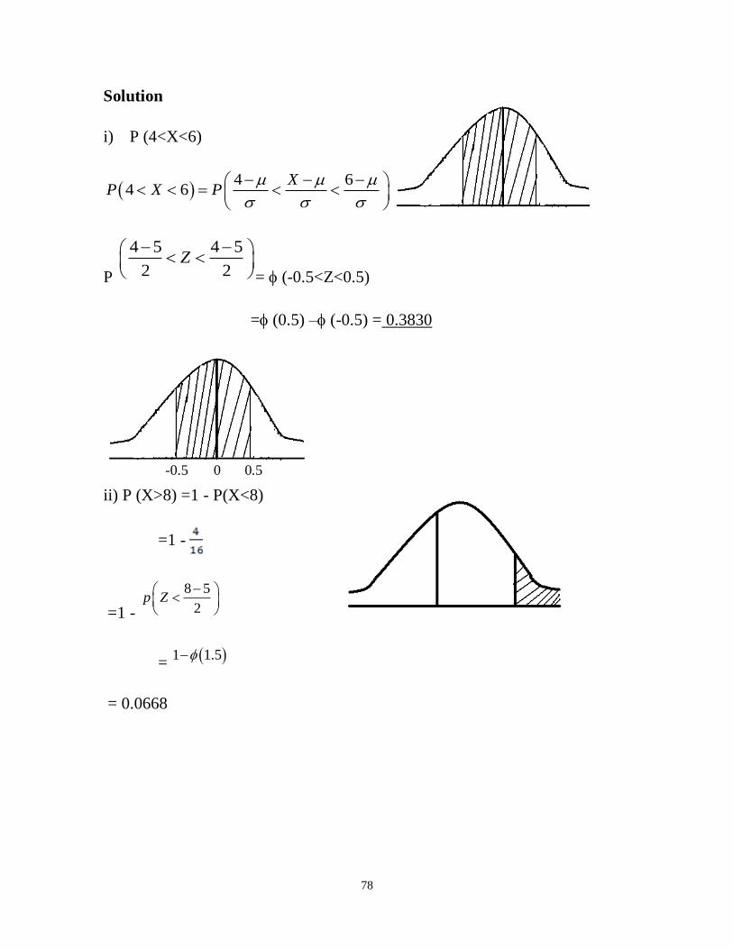
i) P (4<X<6)

4 6

4 6X

P X P

P

4 5 4 5

2 2Z

= (-0.5<Z<0.5)

= (0.5) – (-0.5) = 0.3830

ii) P (X>8) =1 - P(X<8)

=1 -

=1 -

8 5

2p Z

= 1 1.5

= 0.0668

4 5 6

-0.5 0 0.5

0

5 8

79

Example 3

1. If XN (10, 22), find

i) P(7 <X< 13)

ii) P(X > 13)

2. If X N(60, 62), Find

i) P(X=31)

ii) P(|X-60|>9)

3. Suppose that the height of some Students are normally distributed

with mean =65 inches and variance 9 inch squared. What

percentage of them has heights between 59 inches and 71 inches?

Solution

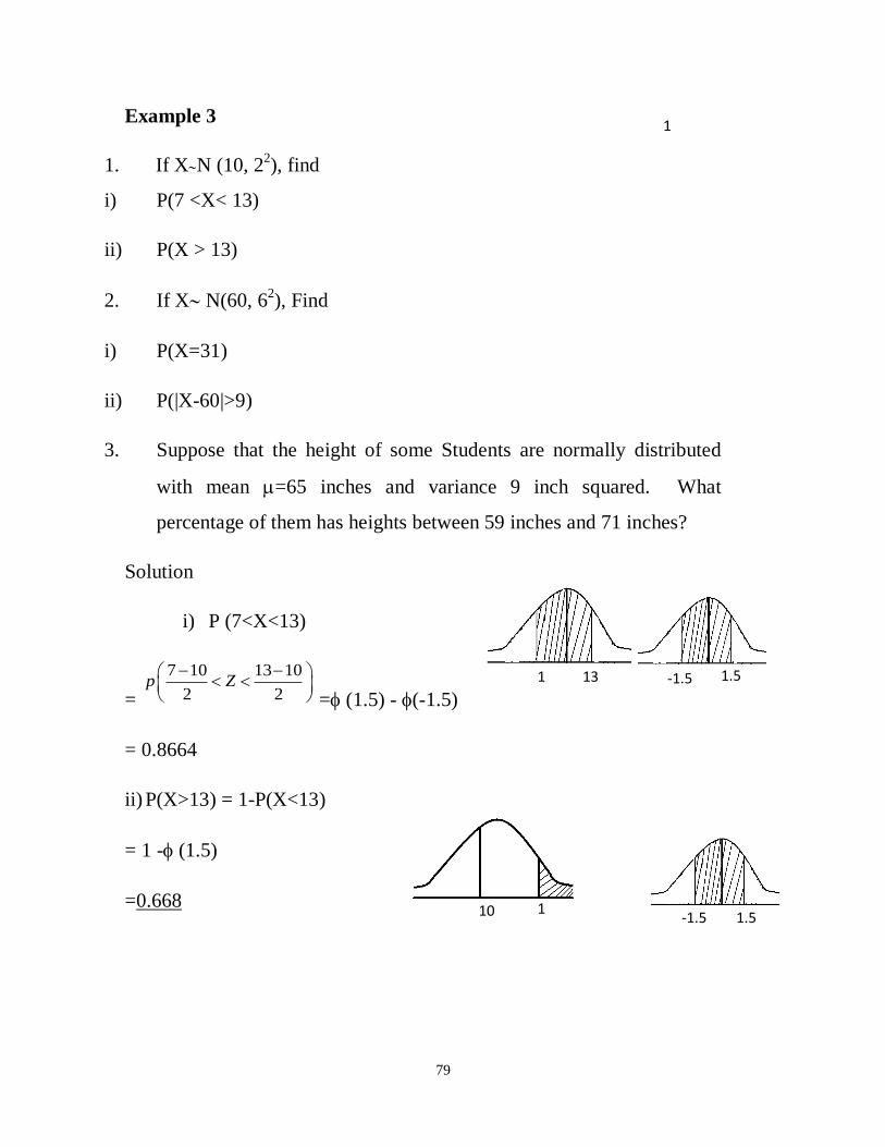
i) P (7<X<13)

=

7 10 13 10

2 2p Z

= (1.5) - (-1.5)

= 0.8664

ii) P(X>13) = 1-P(X<13)

= 1 - (1.5)

=0.668

0 1

.

5

7 1

0

13 -1.5 0 1.5

10 1

3

0 -1.5 1.5

80

2. i) P (Z=31) = 0 for a continuous variable P (X=C)=0

ii) P (X<50) =

54 60

6p Z

= (-1)

=0.1587

iii) |x-60|>9 = (X-60)>9

= X > 69 or

-(X-60)>9 = -X + 60 > 9

=51 > X

Thus | X-60|>9

= X<51 or X > 69

Therefore P (|X-60|> 9)

= P (X > 69) +P (X< 51)

= {1- P (X<69)} + P (X< 51)

=

69 60 51 601

6 6

=1 - (1.5) + (- 1.5)

=1- (1.5) + [1-(1.5)]

51 69

6

0

81

=0.0668 + 0.0668

= 0.1336

3.) X N (65,9)

P (59<X<71) =

71 65

3

-

59 65

3

= (2) - (-2)

= 0.9544

Therefore 95% of the students with heights between 59 inches and 71

inches.

Example 4

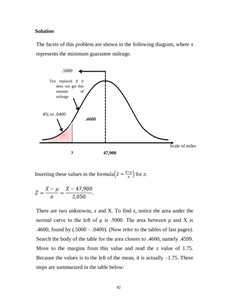
Suppose a tire manufacturer wants to set a minimum mileage guarantee

on its new MX 100 tire. Tests reveal the mean mileage is 47,900 with a

standard deviation of 2,050 miles and a normal distribution. The

manufacturer wants to set the minimum guarantee mileage so that no

more than 4% of the tires will have to be replaced. What minimum

guarantee mileage should the manufacturer announce?

59 65 75

-2 0 2

82

Solution

The facets of this problem are shown in the following diagram, where x

represents the minimum guarantee mileage.

Inserting these values in the formula for z:

There are two unknowns, z and X. To find z, notice the area under the

normal curve to the left of μ is .5000. The area between μ and X is

.4600, found by (.5000 – .0400). (Now refer to the tables of last pages).

Search the body of the table for the area closers to .4600, namely .4599.

Move to the margins from this value and read the z value of 1.75.

Because the values is to the left of the mean, it is actually –1.75. These

steps are summarized in the table below:

Tire replaced if it

does not get this

amount of

mileage

?

.4600

47,900

Scale of miles X μ

4% or .0400

.5000

83

Z .03 .04 .05 .06

… … … … …

1.5 .4370 .4382 .4394 .4406

1.6 .4484 .4382 .4505 .4515

1.7 .4582 .4591 .4599 .4608

1.8 .4664 .4671 .4678 .4686

Knowing that the distance between μ and X is -1.75σ, we can now solve

for X (the minimum guaranteed mileage):

–1.75(2,050) = X – 47,900

X = 47,900 – 1.75(2,050) = 44,312

So the manufacturer can advertise that it will replace for free any tire

that wears out before it reaches 44,312 miles, and the company will

know that only 4 percent of the tires will be replaced under this plan.

84

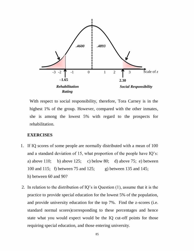
Example 5

Suppose a study of the inmates of a correctional institution is concerned

with the social responsibility of the inmates in prison and their

prospects for rehabilitation upon being released. Each inmate is given a

test regarding social responsibility. The scores are normally distributed,

with a mean of 100 and a standard deviation of 20. Prison psychologists

rated each of the inmates with respect to the prospect for rehabilitation.

These ratings are also normally distributed, with a mean of 500 and a

standard deviation of 100. Tora Carney scored 146 on the social

responsibility test, and her rating with respect to rehabilitation is 335.

How does Tora compare to the group with respect to social

responsibility and the prospect for rehabilitation?

Solution

Converting her social responsibility test score of 146 to a z value using

formula

Converting her rehabilitation rating of 335 to a z value:

The Standardized test score and the standardized rating are shown

below.

85

With respect to social responsibility, therefore, Tora Carney is in the

highest 1% of the group. However, compared with the other inmates,

she is among the lowest 5% with regard to the prospects for

rehabilitation.

EXERCISES

1. If IQ scores of some people are normally distributed with a mean of 100

and a standard deviation of 15, what proportion of the people have IQ‟s:

a) above 110; b) above 125; c) below 80; d) above 75; e) between

100 and 115; f) between 75 and 125; g) between 135 and 145;

h) between 60 and 90?

2. In relation to the distribution of IQ‟s in Question (1), assume that it is the

practice to provide special education for the lowest 5% of the population,

and provide university education for the top 7%. Find the z-scores (i.e.

standard normal scores)corresponding to these percentages and hence

state what you would expect would be the IQ cut-off points for those

requiring special education, and those entering university.

Social Responsibility Rehabilitation

Rating

2.30 –1.65

.4600 .4893

Scale of z -3 -2 -1 0 1 2 3

86

3. The mean diameter of a sample of washers produced by a machine is

5.02mm and the standard deviation is 0.05mm. The tolerance limits of

the diameter is 4.96mm to 5.08mm otherwise it is rejected. It 1000

washers were produced how many would be expected to be rejected?

4. The mass of eggs laid by some hens are normally distributed with mean

60 grams and standard deviation 15 grams. Egg‟s mass less than 45

grams are classified as small. The remainders are divided into standard

and large, and it is desired that these should occur with equal frequency.

Suggest the mass at which the division should be made (correct to the

nearest gram).

5. The weights of bars of soap made in a factory are normally distributed.

Last week 62/3% of bars weighed less than 90.50 grams and 4% weighed

more than 100.25 grams.

Find the mean and variance of the distribution of weights, and the

percentage of bars produced, which would be expected to weigh less than

88 grams.

If the variance of the weight distribution was reduced by one-third, what

percentage of the next week‟s production would you expect to weigh less

than 88 grams, assuming the mean is not changed?

6. The heights of students in Ghana are normally distributed with a mean of

62 inches and a standard deviation of 8 inches. How long should

mattresses produced from a factory be in order to accommodate 95 per

cent of them?

87

7. The weights of some students are normally distributed with mean 80 kg

and a standard deviation 20 kg. The students are classified into groups

A, B and C by weight. 20% of the students belong to group C and

groups A and B have equal proportions of students. Obtain the weights,

which divide the students if those in group A weigh, less than those in

group B and those in group C are the heaviest students.

88

CHAPTER SIX

FORECASTING

INTRODUCTION

Every day, managers make decisions without knowing what will

happen in the future. Inventory is ordered though no one knows what

sales will be, new equipment is purchased though no one knows the

demand for products, and investments are made though no one knows

what profits will be. Managers are always trying to reduce this

uncertainty and to make better estimates of what will happen in the

future. Accomplishing this is the main purpose of forecasting.

There are many ways to forecast the future. In numerous firms

(especially smaller ones), the entire process is subjective, involving

seat-of-the pants methods, intuition, and years of experience. there are

also many quantitative forecasting models, such as moving averages,

exponential smoothing, trend projections, and least squares regression

analysis,

Regardless of the method that is used to make the forecast, the same

eight overall procedures that follow are used.

QUALITATIVE MODELS

Whereas time-series and causal models rely on quantitative data,

qualitative models attempt to incorporate judgmental or subjective

factors into the forecasting model Opinions by experts, individual

experiences and judgments, and other subjective factors may be

considered. Qualitative models are especially useful when subjective

89

factors are expected to be very important or when accurate quantitative

data are difficult to obtain.

Here is a brief overview of four different qualitative forecasting

techniques:

Delphi method: This iterative group process allows experts, who may

be located in different places, to make forecasts. There are three

different types of participants in the Delphi process: decisions makers,

staff personnel, and respondents. The decision making group usually

consists of 5 to 10 experts who will be making the actual forecast. The

staff personnel assist the decision makers by preparing, distributing,

collecting, and summarizing a series of questionnaires and survey

results. The respondents are a group of people whose judgments are

valued and are being sought. This group provides inputs to the decision

makers before the forecasts are made.

Jury of executive opinion: This method takes the opinions of a small

group of high level managers, often in combination with statistical

models, and results in a group estimate of demand.

Sales force composite: In this approach, each salesperson estimates

what sales will be in his or her region; these forecasts are reviewed to

ensure that they are realistic and are then combined at the district and

national levels to reach an overall forecast.

Consumer market survey: This method solicits input from customers

or potential customers regarding their future purchasing plans. It can

help not only in preparing a forecast but also in improving product

design and planning for new products.

90

MEASURES OF FORECAST ACCURACY

We discuss several different forecasting models in this chapter. To see how

well one model works, or to compare with the actual or observed values.

The forecast error (or deviation) is defined as follows:

Forecast error = actual value – forecast value

One measure of accuracy is the mean absolute deviation (MAD). This is

computed by taking the sum of the absolute values of the individual

forecast errors and dividing by the numbers of errors (n);

forecast errorMAD

n

Consider the Wacker Distributors sales of CD players seen in Table 5.1.

Suppose that in the past, Wacker had forecast sales for each year to be

the sales that were actually achieved in the previous year. This is

sometimes called a naïve model. Table 5.2 gives these forecasts as well

as the absolute value of the errors in forecasting for the next time period

(year 11), the forecast would be 190. Notice that there is no error

computed for year 1 since there was no forecast for this year, and there

is no error for year 11 since the actual value of this is not yet known.

Thus, the number of errors (n) is 9.

From this, we see the following:

forecast error 16017.8

9MAD

n

91

This means that on the average, each forecast missed the actual value

by 17.8 units.

YEAR ACTUAL

SALES OF CD

PLAYERS

FORECAST

SALES

ABSOLUTE VALUE

OF ERRORS

(DEVIATION)

[ACTUAL – FORECAST]

1 110 - -

2 100 110 |100-110| = 10

3 120 100 |120-100| = 20

4 140 120 |140-120| = 20

5 170 140 |170-140| = 30

6 150 170 |150-170| = 20

7 160 150 |160-150| = 10

8 190 160 |190-160| = 30

9 200 190 |200-190| = 10

10 190 200 |190-200| = 10

11 - 190 -

Sum of |errors| =

160

MAD = 160/9 =

17.8

92

There are other measures of the accuracy of historical errors in

forecasting that are sometimes used besides the MAD. One of the most

common is the mean squared error (MSE) which is the average of the

squared errors:

2

errorsMSE

n

Besides the MAD and MSE, the mean absolute percent error (MAPE) is

sometimes used. The MAPE is the average of the absolute values of the

errors expressed as percentages of the actual values. This is computed as

follows:

| |

100%

error

actualMAPEn

There is another common term associated with error in forecasting. Bias

is the average error and tells whether the forecast tends to be too high or

too low and by how much. Thus, bias may be negative or positive. It is

not a good measure of the actual size of the errors because the negative

errors can cancel out the positive errors.

Moving Averages

Moving averages are useful if we can assume that market demands will

stay fairly steady over time. For example, a four months and dividing

by 4. With each passing month, the most recent month‟s data are added

to the sum of the previous three months‟ data, and the earliest month is

dropped. This tends to smooth out short-term irregularities in the data

93

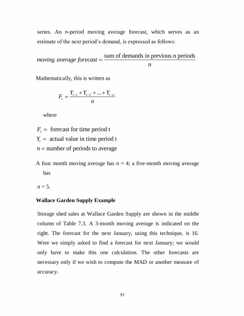
series. An n-period moving average forecast, which serves as an

estimate of the next period‟s demand, is expressed as follows:

sum of demands in previous n periods moving average forecast

n

Mathematically, this is written as

1 2 ...t t t n

t

Y Y YF

n

where

forecast for time period t

actual value in time period t

number of periods to average

t

t

F

Y

n

A four month moving average has n = 4; a five-month moving average

has

n = 5.

Wallace Garden Supply Example

Storage shed sales at Wallace Garden Supply are shown in the middle

column of Table 7.3. A 3-month moving average is indicated on the

right. The forecast for the next January, using this technique, is 16.

Were we simply asked to find a forecast for next January; we would

only have to make this one calculation. The other forecasts are

necessary only if we wish to compute the MAD or another measure of

accuracy.

94

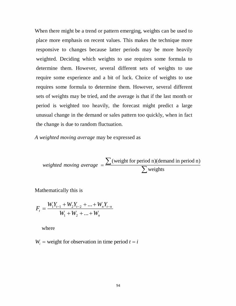
When there might be a trend or pattern emerging, weights can be used to

place more emphasis on recent values. This makes the technique more

responsive to changes because latter periods may be more heavily

weighted. Deciding which weights to use requires some formula to

determine them. However, several different sets of weights to use

require some experience and a bit of luck. Choice of weights to use

requires some formula to determine them. However, several different

sets of weights may be tried, and the average is that if the last month or

period is weighted too heavily, the forecast might predict a large

unusual change in the demand or sales pattern too quickly, when in fact

the change is due to random fluctuation.

A weighted moving average may be expressed as

(weight for period n)(demand in period n)

weightsweighted moving average

Mathematically this is

1 1 2 2

1 2

...

...

t t n t n

t

n

W Y W Y W YF

W W W

where

weight for observation in time period iW t i

95

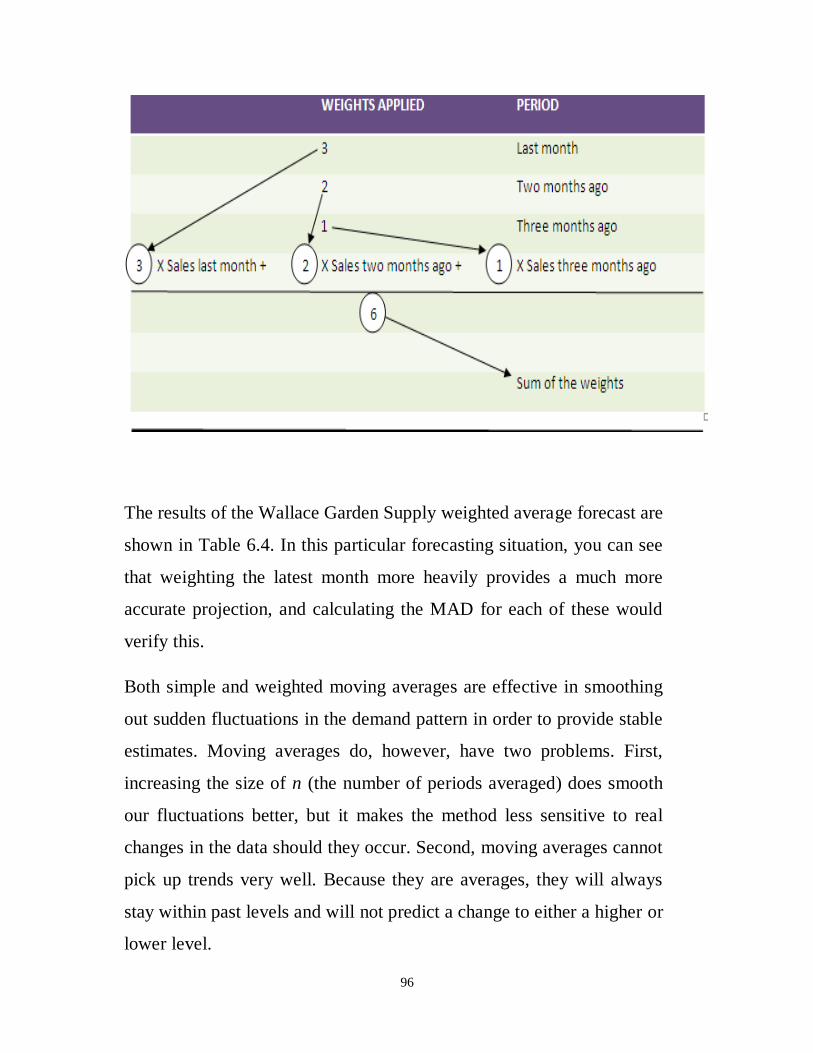
Wallace Garden Supply decides to forecast storage shed sales by

weighing the past three months as follows:

96

The results of the Wallace Garden Supply weighted average forecast are

shown in Table 6.4. In this particular forecasting situation, you can see

that weighting the latest month more heavily provides a much more

accurate projection, and calculating the MAD for each of these would

verify this.

Both simple and weighted moving averages are effective in smoothing

out sudden fluctuations in the demand pattern in order to provide stable

estimates. Moving averages do, however, have two problems. First,

increasing the size of n (the number of periods averaged) does smooth

our fluctuations better, but it makes the method less sensitive to real

changes in the data should they occur. Second, moving averages cannot

pick up trends very well. Because they are averages, they will always

stay within past levels and will not predict a change to either a higher or

lower level.

97

Exponential Smoothing

Exponential smoothing is a forecasting method that is easy to use and is

handled efficiently by computers. Although it is a type of moving

average technique, it involves little record keeping of past data. The

basic exponential smoothing formula can be shown as follows:

New forecast = last period’s forecast + α (last period’s actual

demand – last period’s forecast)

Where α is a weight (or smoothing constant) that has a value between

0 and 1, inclusive.

Equation for determining forecast using exponential smoothing can

be written mathematically as

98

Ft = Ft-1 + α (Yt-1 – Ft-1)

Where

Ft = new forecast (for time period t)

Ft-1 = previous forecast (for time period t - 1)

α = smoothing constant (0 ≤ α ≤ 1)

Yt-1 = previous periods actual demand

The concept here is not complex. The latest estimate of demand is equal

to the old estimate adjusted by a fraction of the error (last period‟s

actual demand minus the old estimate).

The smoothing constant, α, can be changed to give more weight to

recent data when the value is high or more weight to past data when it is

low. For example, when α = 0.5, it can be shown mathematically that

the new forecast is base almost entirely on demand in the past three

periods. When α = 0.1, forecast places little weight on the single period,

even the most recent, and it takes many periods (about 19) of historic

values into account.

In January, a demand for 142 of a certain car model for February was

predicted by a dealer. Actual February demand was 153 autos. Using a

smoothing constant of α = 0.20, we can forecast the March mean using

the exponential smoothing model. Substituting into the formula, we

obtain

New forecast (for March demand) = 142+ 0.2(153-142)

= 144.2

99

Thus, the demand forecast for the cars in March was 136. A forecast for

the demand in April, using the exponential smoothing model with a

constant of α = 0.20, can be made:

New forecast (for April demand) = 144.2 + 0.2(136-144.2)

= 142.6 or 143 autos

Selecting the smoothing constant

The exponential smoothing approach is easy to use and has been

applied successfully by banks, manufacturing companies, wholesalers,

and other organizations. The appropriate value of the smoothing

constant, α, however, can value for the smoothing constant, the

objective is to obtain the most accurate forecast. Several values of the

smoothing constant may be tried, and the one with the lowest MAD

could be selected. This is analogous to how weights are selected for a

weighted moving constant. QM for windows will display the MAD that

would be obtained with values of α ranging from 0 to 1 increments of

0.01.

Port of Baltimore Example

Let us apply this concept with a trial-and-error testing for two values of

α in the following example. The port of Baltimore has unloaded large

quantities of grain from ships during the past eight quarters. The port‟s

operations manger wants to test the use of exponential smoothing to see

how well the technique works in predicting tonnage unloaded. He

assumes that the forecast of grain unloaded in the first quarter was 175

100

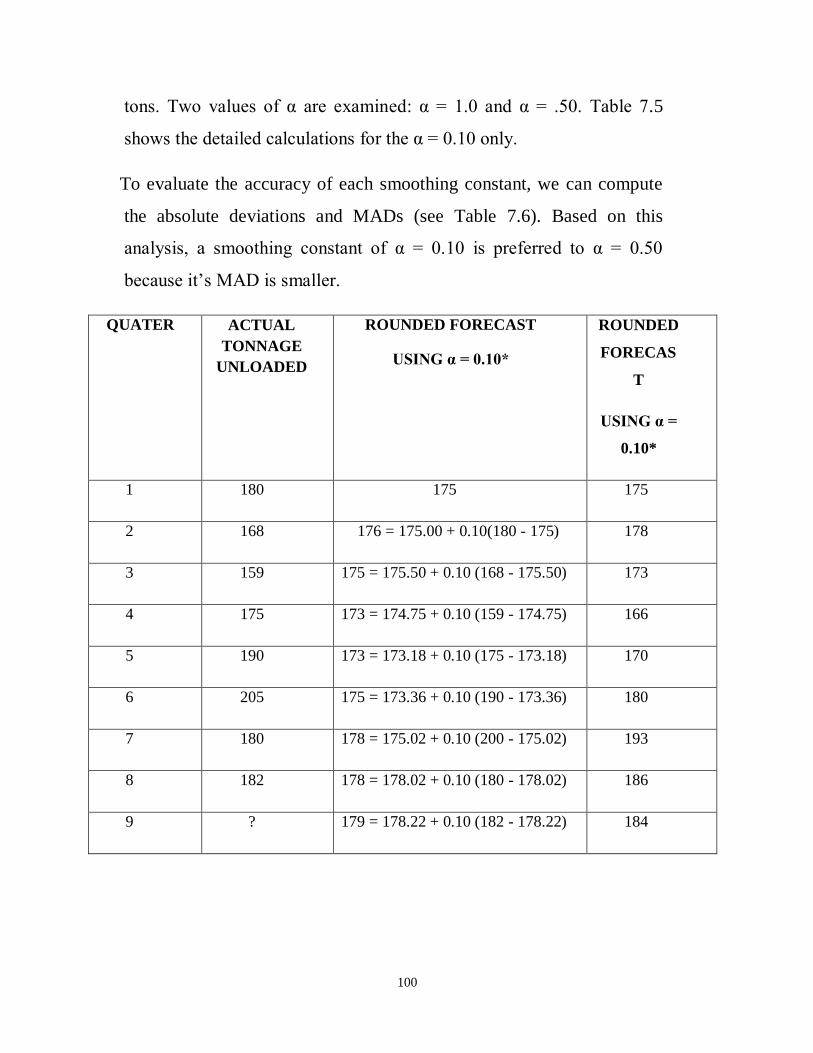
tons. Two values of α are examined: α = 1.0 and α = .50. Table 7.5

shows the detailed calculations for the α = 0.10 only.

To evaluate the accuracy of each smoothing constant, we can compute

the absolute deviations and MADs (see Table 7.6). Based on this

analysis, a smoothing constant of α = 0.10 is preferred to α = 0.50

because it‟s MAD is smaller.

QUATER ACTUAL

TONNAGE

UNLOADED

ROUNDED FORECAST

USING α = 0.10*

ROUNDED

FORECAS

T

USING α =

0.10*

1 180 175 175

2 168 176 = 175.00 + 0.10(180 - 175) 178

3 159 175 = 175.50 + 0.10 (168 - 175.50) 173

4 175 173 = 174.75 + 0.10 (159 - 174.75) 166

5 190 173 = 173.18 + 0.10 (175 - 173.18) 170

6 205 175 = 173.36 + 0.10 (190 - 173.36) 180

7 180 178 = 175.02 + 0.10 (200 - 175.02) 193

8 182 178 = 178.02 + 0.10 (180 - 178.02) 186

9 ? 179 = 178.22 + 0.10 (182 - 178.22) 184

101

Using Excel QM for exponential Smoothing Programs 6.2A and

Programs 6.2B illustrate how Excel QM handles exponential

smoothing. Input data and formulas appear in Program 6.2A and output,

using α of 0.1 for the port of Baltimore, are in Program 6.2B. Note that

the MAD in (of 10.307) differs slightly from that in Table 6.6 because

of rounding.

Decision–Making Group: A group of experts in a Delphi technique that

has the responsibility of making the forecast.

QUARTER ACTUAL

TONAGE

UNLOADED

ROUNDED

FORECAST

WITH 0.10

ABSOLUTE

DEVIATIONS

FOR 0.10

ROUNDED

FORCAST

WITH 0.50

ABSOLUTE

DEVIATIONS

FOR 0.50

1 180 175 5 175 5

2 168 176 8 178 10

3 159 175 16 173 14

4 175 173 2 166 9

5 190 173 17 170 20

6 205 175 30 180 25

7 180 178 2 193 13

8 182 178 4 186 4

Sum of

absolute

deviations

84 100

MAD = 12.50

102

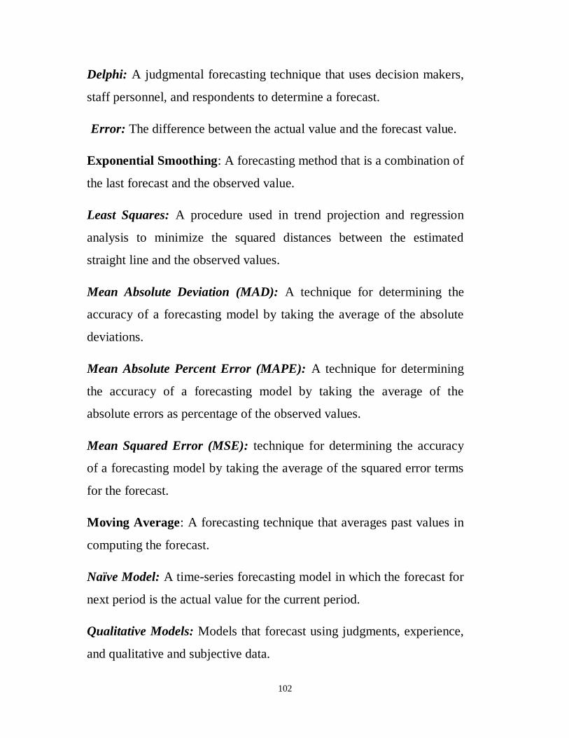
Delphi: A judgmental forecasting technique that uses decision makers,

staff personnel, and respondents to determine a forecast.

Error: The difference between the actual value and the forecast value.

Exponential Smoothing: A forecasting method that is a combination of

the last forecast and the observed value.

Least Squares: A procedure used in trend projection and regression

analysis to minimize the squared distances between the estimated

straight line and the observed values.

Mean Absolute Deviation (MAD): A technique for determining the

accuracy of a forecasting model by taking the average of the absolute

deviations.

Mean Absolute Percent Error (MAPE): A technique for determining

the accuracy of a forecasting model by taking the average of the

absolute errors as percentage of the observed values.

Mean Squared Error (MSE): technique for determining the accuracy

of a forecasting model by taking the average of the squared error terms

for the forecast.

Moving Average: A forecasting technique that averages past values in

computing the forecast.

Naïve Model: A time-series forecasting model in which the forecast for

next period is the actual value for the current period.

Qualitative Models: Models that forecast using judgments, experience,

and qualitative and subjective data.

103

Smoothing Constant: A value between 0 and 1 that is used in an

exponential smoothing forecast.

Weighted Moving Average: A moving average forecasting method that

places different weights on past values.

SOLVED PROBLEMS

Demand for patient surgery at Washington General Hospital has

increased steadily in the past few years as seen in the following table.

YEAR OUTPATIENT

SURGERIES

PERFORMED

1 45

2 50

3 52

4 56

5 58

6 -

The director of medical services predicted six years ago that demand in

year 1 would be 42 surgeries. Using exponential smoothing with a

104

weight of =0.20, develop forecasts for years 2 through 6. What is the

MAD?

YEAR ACTUAL FORECAST

(SMOOTHED)

ERROR |ERROR|

1 45 42 +3 3

2 50 42.6=42+0.2(45-42) +7.4 7.4

3 52 44.1=42.6+0.2(50-42.6) +7.9 7.9

4 56 45.7=44.1+0.2(52-44.1) +10.3 10.3

5 58 47.7=45.7+0.2(56-45.7) - -

6 - 49.8=47.7+.2(58-47.7) - -

38.9

PROBLEMS

1. Develop a four-month moving average forecast for Wallace Garden

Supply and compute the MAD. A three-month moving average

forecast was developed in the section on moving averages in Table

6.3.

2. Using MAD, determine whether the forecast in Problems 6-12 or the

forecast in the section concerning Wallace Garden Supply is more

accurate.

105

3. Data collected on the yearly demand for 50-pound bags of fertilizer at

Wallace Garden Supply are shown in the following table. Develop a

three-year moving average to forecast sales. Then estimate demand

again with a weighted moving average in which sales in the most

recent year are given a weight of 2 and sales in the other two years

are each given a weight of 1. Which method do you think is?

YEAR DEMAND FOR

FERTILIZER

(1,000s of Bags)

1 4

2 6

3 4

4 5

5 10

6 8

7 7

8 9

9 12

10 14

11 15

106

4. Use exponential smoothing with a smoothing constant of 0.3 to

forecast the demand for fertilizer given in Problem 6.14.Assume that

the last period‟s forecast for year 1 is 5000 bags to begin the

procedure. Would you prefer to use the exponential smoothing model

or the weighted average model developed on Problem 3.

5. Sales of Cool-Man air conditioners have grown steadily during the

past five years.

YEAR SALES

1 450

2 495

3 518

4 563

5 584

6 ?

The Sales manager had predicted, before the business started, that year

1‟s sales would be 410 air conditioners. Using exponential smoothing

with a weight of α = 0.30, develop forecasts for years 2 through 6.

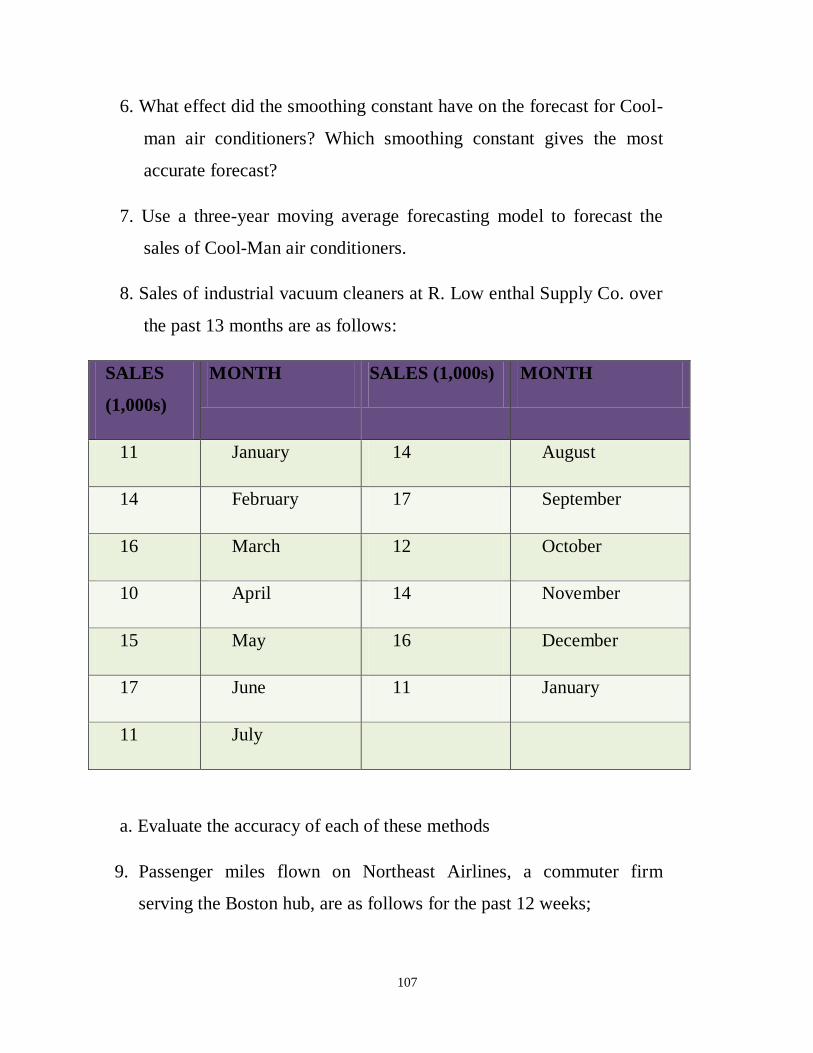
107

6. What effect did the smoothing constant have on the forecast for Cool-

man air conditioners? Which smoothing constant gives the most

accurate forecast?

7. Use a three-year moving average forecasting model to forecast the

sales of Cool-Man air conditioners.

8. Sales of industrial vacuum cleaners at R. Low enthal Supply Co. over

the past 13 months are as follows:

SALES

(1,000s)

MONTH SALES (1,000s) MONTH

11 January 14 August

14 February 17 September

16 March 12 October

10 April 14 November

15 May 16 December

17 June 11 January

11 July

a. Evaluate the accuracy of each of these methods

9. Passenger miles flown on Northeast Airlines, a commuter firm

serving the Boston hub, are as follows for the past 12 weeks;

108

WEEK ACTUAL PASSENGER

(1,000s)

1 17

2 21

3 19

4 23

5 18

6 16

7 20

8 18

9 22

10 20

11 15

12 22

10. Emergency calls to Winter Park, Florida‟s 911 system, for past 24

weeks are as follows:

109

WEEK CALLS WEEK CALLS

1 50 13 55

2 35 14 35

3 25 15 25

4 40 16 55

5 45 17 55

6 35 18 40

7 20 19 35

8 30 20 60

9 35 21 75

10 20 22 50

11 15 23 40

12 40 24 65

a. Compare the exponentially smoothed forecast of calls for each

week. Assume an initial forecast of 50 calls in the first week and use

α = 0.1. What is the forecast for the 25th

week?

b. Reforecast each period using α = 0.6

c. Actual calls during the 25th

week were 85. Which smoothing

constant provides a superior forecast?

110

11. Using the 911 call data in Problem 9, forecast calls for weeks 2

through 25 using α = 0.9. Which is best? (Again, assume that actual

calls in week 25 were 85 and use an initial forecast of 50 calls.)

12. Consulting income at Kate Walsh Association for the period

February-July has been as follows:

MONTH INCOME(1,000s)

February 70.0

March 68.5

April 64.8

May 71.7

June 71.3

July 72.8

Use exponential smoothing to forecast Augusts‟ income. Assume that

the initial forecast for February is $65,000. The smoothing constant

selected is α = 0.1.

Resolve Problem 12 with α = 0.3. Using MAD, which smoothing constant

provides a better forecast?

111

CHAPTER SEVEN

MATRICES AND ITS APPLICATIONS

INTRODUCTION

A business may collect and store or analyze various types of data as a

regular part of its record-keeping procedures. The data may be

presented in tabular form.

For example, a store owner who sells different building materials may

want to know his/her daily sales from each of the building materials.

Table 1

If we write the numbers from table 1 in the rectangular array

1200 7350 700

950 8000 980P

We say that P is a matrix (plural: matrices) representing table 1.

In addition to storing data in a matrix, we can analyze data and make

business decisions by defining the operations of addition, subtraction

and multiplication for matrices.

112

In general, we define a matrix as any rectangular array of

numbers/elements. The numbers in a matrix are called a matrix its

entries or elements

Example of matrices is:

23

12

(12 11)

2 3

3 5

2 1 5

3 4 1

3 5 6

A

B

C

D

SIZE OF A MATRIX

The size of a matrix is determined by its number of rows by the number

of columns

23The matrix , has 2 rows and 1 column

12

Therefore is a 2 1 matrix

A

A

The matrix (1 3 7), has 1 row and 3 columns

Therefore is a 1 3 matrix

2 4The matrix , has 2 rows and 2 columns

1 3

Therefore is a 2 2 matrix

3 1 5The matrix , has 2 rows and 3 columns

2 3 7

The

B

B

C

C

D

refore is a 2 3 matrixD

113

If the number of rows of a matrix equals the number of columns, we say

the matrix is a square matrix

ADDITION AND SUBTRACTION OF MATRICES

We can only add or subtract matrices which are of the same dimension

(size)

Example 1

Given that

3 5 2 3 and , find

1 7 3 4A B A B

Solution

3 5 2 3

1 7 3 4

3 2 5 3

1 3 7 4

5 8

4 11

A B

Example 2

Given that

2 5 3 3 4 1 and , find

3 6 2 1 2 2C D C D

114

Solution

4 5 3 3 4 1

3 6 2 1 2 2

4 3 5 4 3 1

3 1 6 2 2 2

1 1 2

2 4 0

C D

MULTIPLICATION OF MATRICES BY SCALAR

When a matrix is multiplied by a scalar k, we use the scalar to multiply

each of the elements in the matrix.

If , then a b a b

P kP kc d c d

ka kb

kc kd

Example 3

Given that

3 5 2 3 and , find 2 3

1 4 1 6M N M N

Solution

115

3 5 2 32 3 2 3

1 4 1 6

6 10 6 9

2 8 3 18

6 6 10 9

2 3 8 18

12 19

5 26

M N

Example 4

Given that

2 1 3 2

3 2 and 1 3 , find 4 3

4 2 3 5

M N N M

Solution

3 2 2 1

4 3 4 1 3 3 3 2

3 5 4 2

12 8 6 3

4 12 9 6

12 20 12 6

12 6 8 3 6 5

4 9 12 6 5 6

12 12 20 6 0 14

N M

116

Example 5

The total sales in cedis made by two shops „God Reigns‟ and „Good

Father‟ on goods sold in the months of April and May is as shown below.

(a) What was the combined cedi sale from the months of April and

May?

(b) What was the increase in the cedi sales from April to May?

(c) If both shops received 10% increase in sales in the month of June

from May sales and had 5% decrease in July sales from June sales,

compute the total sales from the months of June and July.

Solution

6000 3200 6500 4200,

4500 3200 5000 4000

6000 3200 6500 4200(a)

4500 3200 5000 4000

6000 6500 3200 4200

4500 5000 3200 4000

12500 7400

9500 7200

A B

A B

117

6500 4200 6000 3200(b)

5000 4000 4500 3200

6500 6000 4200 3200

5000 4500 4000 3200

500 1000

500 800

B A

6500 4200(c) June : 1.1

5000 4000

7150 4620

5500 4400

C

7150 4620July: 0.95

5500 4400

6792.5 4389

5225 4180

D

7150 4620 6792.5 4389

5500 4400 5225 4180

13942 9009

10725 8580

C D

MULTIPLICATION OF MATRICES

Two matrices can be multiplied if the number of rows of the first matrix

is equal to the number of columns of the second matrix.

If matrix A has size m × n and matrix B has size n × p, then the matrix

AB can be multiplied with size m × p

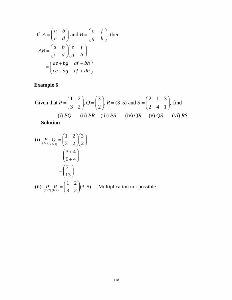
118

If and , thena b e f

A Bc d g h

a b e fAB

c d g h

ae bg af bh

ce dg cf dh

Example 6

1 2 3 2 1 3Given that , , (3 5) and , find

3 2 2 2 4 1

(i) (ii) (iii) (iv) Q (v) (vi)

P Q R S

PQ PR PS R QS RS

Solution

(2 2) (2 1)

(2 2) (1 2)

1 2 3(i)

3 2 2

3 4

9 4

7

13

1 2(ii) (3 5) [Multiplication not possible]

3 2

P Q

P R

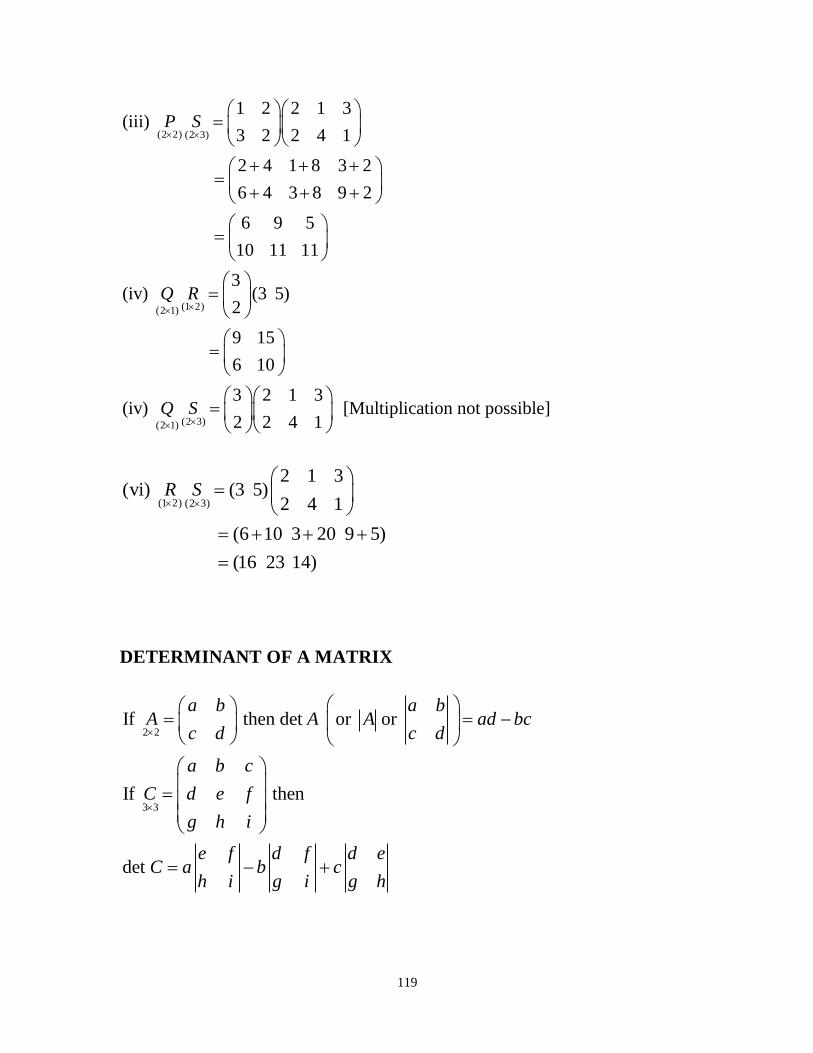
119

(2 2) (2 3)

(1 2)(2 1)

(2 3)(2 1)

1 2 2 1 3(iii)

3 2 2 4 1

2 4 1 8 3 2

6 4 3 8 9 2

6 9 5

10 11 11

3(iv) (3 5)

2

9 15

6 10

3 2 1 3(iv) [Multiplication not possible]

2 2 4 1

P S

Q R

Q S

(1 2) (2 3)

2 1 3(vi) (3 5)

2 4 1

(6 10 3 20 9 5)

(16 23 14)

R S

DETERMINANT OF A MATRIX

2 2

3 3

If then det or or

If then

det

a b a bA A A ad bc

c d c d

a b c

C d e f

g h i

e f d f d eC a b c

h i g i g h

120

OR we can also find the determinant of a 3×3 matrix by

1. First writing the matrix without the bracket

2. Adjoin the matrix with the first two columns of the same matrix and

find the determinant as shown below.

Determinant = sum of the product of downward arrows – sum of the

product of the upward arrows.

Example 7

3 2If , find the determinant of

1 2A A

Solution

3 2 1 2

6 2

4

A

Example 8

2 1 1

If 2 3 5 , find the determinant of

2 1 4

P P

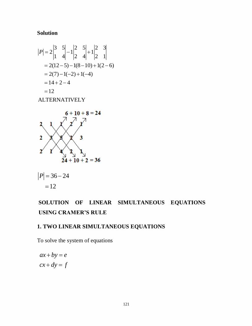
121

Solution

3 5 2 5 2 32 1 1

1 4 2 4 2 1

2(12 5) 1(8 10) 1(2 6)

2(7) 1( 2) 1( 4)

14 2 4

12

ALTERNATIVELY

P

36 24

12

P

SOLUTION OF LINEAR SIMULTANEOUS EQUATIONS

USING CRAMER’S RULE

1. TWO LINEAR SIMULTANEOUS EQUATIONS

To solve the system of equations

ax by e

cx dy f

122

We first rewrite the equations as

Represent the left hand matrix by a letter say and the right hand side matrix

by say

ax by e

cx dy f

a b x e

c d y f

a bA

c d

eB

f

To find , replace the first column of by , find its determinant and divide the results

by the determinant of

Thus:

To find , replace the second column of by , find its determinant and

x A B

A

e b

f dx

A

y A B

divide the results

by the determinant of

Thus:

A

a e

c fy

A

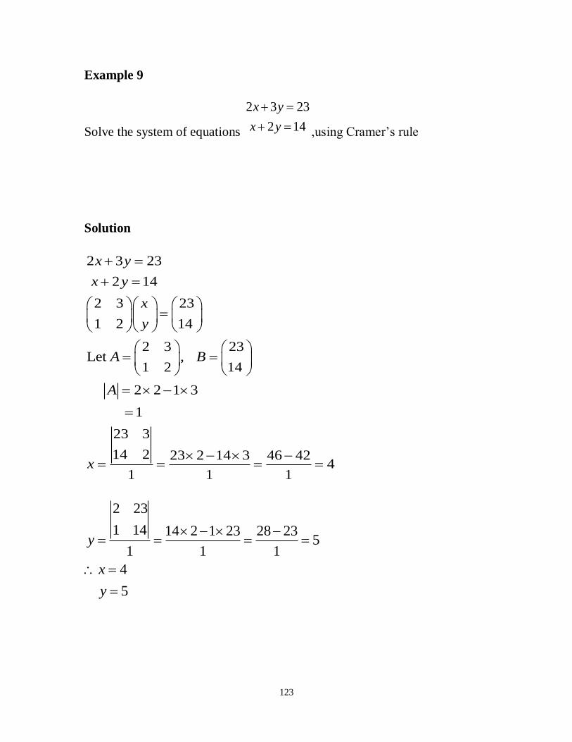
123

Example 9

Solve the system of equations

2 3 23

2 14

x y

x y

,using Cramer‟s rule

Solution

2 3 23

2 14

2 3 23

1 2 14

2 3 23Let ,

1 2 14

2 2 1 3

1

23 3

14 2 23 2 14 3 46 424

1 1 1

x y

x y

x

y

A B

A

x

2 23

1 14 14 2 1 23 28 235

1 1 1

4

5

y

x

y

124

Example 10

Pascal‟s logistics company has an order for two products to be

delivered to two stores. The matrix below gives information regarding

the two products

If a truck can carry 2350 cu ft and 23,000 lb, how many of each product

can it carry.

Solution

Let x = the number of product I it can carry

y = the number of product II it can carry

125

20 30 2350

100 400 23000

20 30 2350

100 400 23000

20 30 2350Let ,

100 400 23000

20 400 100 30

5000

2350 30

23000 400 2350 400 23000 30

5000 5000

940,000 690,000

5000

50

20 2350

x y

x y

x

y

A B

A

x

y

100 23000 23000 20 100 2350

500 500

460,000 235,000

500

450

50

450

x

y

2. THREE LINEAR SIMULTANEOUS EQUATIONS

To solve the system of equations

ax by cz p

dx ey fz q

gx hy ix r

We first rewrite the equations as

126

ax by cz p

dx ey fz q

gx hy iz r

a b c x p

d e f y q

g h i z r

Represent the left hand matrix by a letter say and the right hand side matrix

by say

a b c

A d e f

g h i

p

B q

r

To find , replace the first column of by , find its determinant and divide the results

by the determinant of

Thus:

To find , replace the second column of by , find its determinant

x A B

A

p b c

q e f

r h ix

A

y A B

and divide the results

by the determinant of

Thus:

To find , replace the third column of by , find its determinant and divide the results

by the determinant of

A

a p c

d q f

g r iy

A

z A B

A

127

Thus:

a b p

d e q

g h rz

A

Example 8

Solve the system of equations

1 2 3

1 2 3

1 2 3

3 2 14

5 2 13

2 4 13

X X X

X X X

X X X

,using Cramer‟s rule

Solution

1 2 3

1 2 3

1 2 3

1

2

3

3 2 14

5 2 13

2 4 13

1 3 2 14

5 2 1 13

2 1 4 13

1 3 2 14

Let 5 2 1 , 13

2 1 4 13

X X X

X X X

X X X

X

X

X

M N

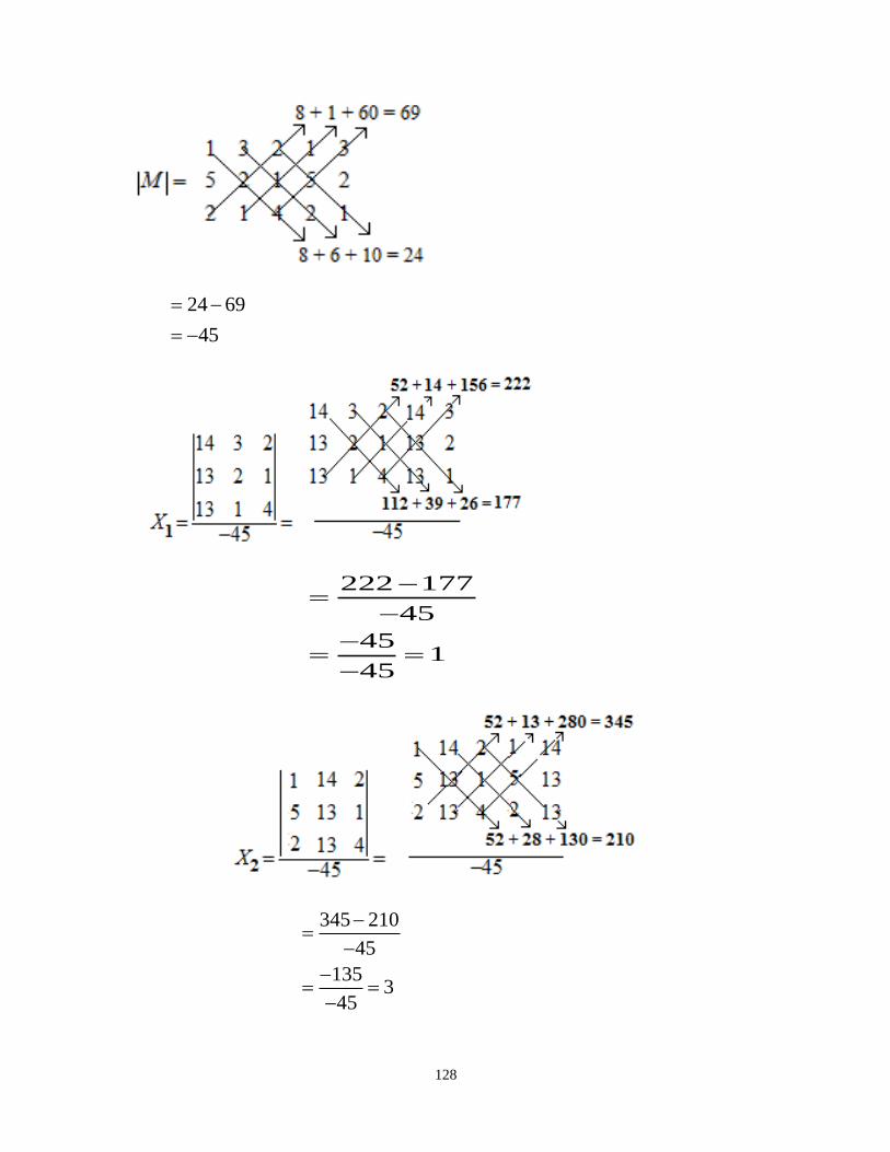
128

24 69

45

222 177

45

451

45

345 210

45

1353

45

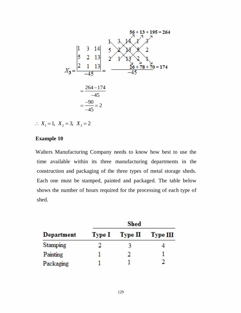
129

264 174

45

902

45

1 2 31, 3, 2X X X

Example 10

Walters Manufacturing Company needs to know how best to use the

time available within its three manufacturing departments in the

construction and packaging of the three types of metal storage sheds.

Each one must be stamped, painted and packaged. The table below

shows the number of hours required for the processing of each type of

shed.

130

Determine how many of each type of shed can be produced if the

stamping department has 3200 hours available, the painting department

has 1700 hours, and the packaging department has 1300 hours.

Solution

Let X be the number of type I sheds, Y be the number of type II sheds

and Z be the number of type III sheds.

The equation 2 3 4 3200X Y Z represents the hours used by the

stamping department.

Similarly;1 2 1 1700X Y Z represents the hours used by the painting

department and 1 1 2 1300X Y Z represents the hours used by the

stamping department

2 3 4 3200

1 2 1 1700

1 1 2 1300

2 3 4 3200

1 2 1 1700

1 1 2 1300

2 3 4 3200

Let 1 2 1 , 1700

1 1 2 1300

X Y Z

X Y Z

X Y Z

X

Y

Z

P Q

131

15 16

1

23800 23500

1

300

1

300

15800 15200

1

600

1

600

132

13700 13500

1

200

1

200

Therefore, the company should make 300 type I, 600 type II and 200

type III sheds

EXERCISES

1. Given that

3 5 2 3 5 7, and find

1 7 3 4 4 3A B C

(i)

(ii)

(iii)

A B

A C B

B C A

2. Given that

3 3 2 4 7 3

1 4 2 and 5 6 9 , find

3 1 1 4 3 3

C D

(i)

(ii)

C D

D C

3. Given that

3 3 5 2 4 3 1 3 2, and find

1 4 2 3 2 4 2 5 3A B C

133

(i) 3

(ii) 2

(iii) 3

(iv) 2

A B

A B C

C A B

B C A

4. The total number of furniture made by two shops „Lom Na Va‟ and

„Saviour‟ in the months of July and August is as shown below.

(a) What was the combined furniture made from the months of July and

August?

(b) What was the increase in the cedi sales from April to May?

(c) If both shops had 15% increases in production in the month of

September from August production and had 10% increase in October

from July production, compute the total production from the months

of September and October.

3 4 4 3 2 15. Given that , , (2 7) and , find

2 1 1 5 3 6

(a) (b) (c) (d) (e) (f)

(g) (h) (i) ( j) (k)

A B C D

AB BA AC CA AD DA

BC CB BD DB CD

6. Find the determinant of each of the following matrices

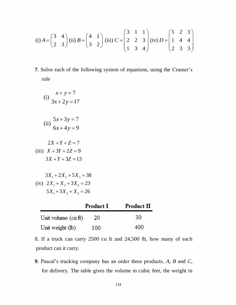
134

3 1 1 5 2 33 4 4 1

(i) (ii) (iii) 2 2 3 (iv) 1 4 42 3 3 2

1 3 4 2 3 3

A B C D

7. Solve each of the following system of equations, using the Cramer‟s

rule

7(i)

3 2 17

5 3 7(ii)

6 4 9

x y

x y

x y

x y

1 2 3

1 2 3

1 2 3

2 7

(iii) 3 2 9

3 3 13

3 2 5 38

(iv) 2 3 23

5 3 26

X Y Z

X Y Z

X Y Z

X X X

X X X

X X X

8. If a truck can carry 2500 cu ft and 24,500 lb, how many of each

product can it carry.

9. Pascal‟s trucking company has an order three products, A, B and C,

for delivery. The table gives the volume in cubic feet, the weight in

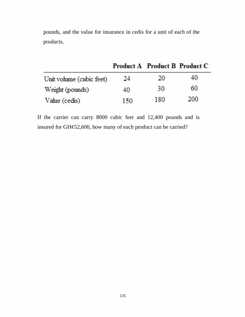
135

pounds, and the value for insurance in cedis for a unit of each of the

products.

If the carrier can carry 8000 cubic feet and 12,400 pounds and is

insured for GH¢52,600, how many of each product can be carried?