Is there Life after Zeno?Taking Executions Past the Breaking (Zeno) Point

Aaron D. Ames, Haiyang Zheng, Robert D. Gregg and Shankar SastryDepartment of Electrical Engineering and Computer Sciences

University of California at BerkeleyBerkeley, CA 94720

{adames,hyzheng,rdgregg,sastry }@eecs.berkeley.edu

Abstract— Understanding Zeno phenomena plays an impor-tant role in understanding hybrid systems. A natural—andintriguing—question to ask is: what happens after a Zenopoint? Inspired by the construction of [9], we propose a methodfor extending Zeno executions past a Zeno point for a classof hybrid systems: Lagrangian hybrid systems. We argue thatafter the Zeno point is reached, the hybrid system should switchto a holonomically constrained dynamical system, where theholonomic constraints are based on the unilateral constraintson the configuration space that originally defined the hybridsystem. These principles are substantiated with a series ofexamples.

I. I NTRODUCTION

Zeno behavior occurs in hybrid systems when there arean infinite number of discrete transitions in a finite periodof time. Since each discrete transition takes a finite (andnonzero) amount of computation time, Zeno behavior pre-vents a simulation from progressing past a certain time, i.e.,the simulator “breaks.” Because the physical system that thehybrid system is modeling can exist past the Zeno point, thesimulator should be able to correctly predict this “life afterZeno.” This motivates the need to carry a Zeno execution(or trajectory) past the point at which Zeno occurs: the Zenopoint.

In this paper, we propose a method for carrying executionspast the Zeno point. Although we do notprove that thisis the correct way to carry executions beyond Zeno points,we argue that our method correctly represents the physical,post-Zeno, behavior of the system being modeled. In order tosupport this argument, we consider a class of hybrid systemsin which we can make inferences about the behavior of thesystems after the Zeno point based on their mathematicalstructure—hybrid systems obtained from (simple)hybridLagrangians: Lagrangian hybrid systems.

A hybrid Lagrangian consists of a configuration space,a Lagrangian, and a unilateral constraint defining the setof admissible configurations of the system (and usuallydictated by physical constraints on the system). From ahybrid Lagrangian, we are able to explicitly construct aLagrangian hybrid system. Hybrid systems of this form aregeneral enough to model a wide range of physical systems(cf. [7] and the more than 1000 references therein), while

*This research is supported by the National Science Foundation (NSFaward number CCR-0225610)

being concrete enough to allow for analysis, e.g., [4] and [5]study how to reduce these systems.

Using the special structure of Lagrangian hybrid systemsobtained from hybrid Lagrangians, we are able to demon-strate that the Zeno point must satisfy constraints imposedby the unilateral constraint function. These constraints areholonomic in nature, and this implies thatafter the Zenopoint the hybrid system should switch to a holonomicallyconstrained dynamical system. The resulting system obtainedby “composing” the hybrid system with this dynamicalsystem defines acompleted hybrid system, which inherentlyallows an execution to continue past the Zeno point. Sincethe Zeno point will never be reached in a simulation environ-ment, we discuss how to practically implement a completedhybrid system, and we illustrate these concepts with a seriesof examples.

II. H YBRID LAGRANGIANS

In this section, we introduce the notion of a hybridLagrangian. Many different forms of “hybrid Lagrangians”have appeared in the literature, although not under thisspecific name. The goal of the definition introduced hereis to be general enough to include these definitions, whilebeing specific enough to allow for explicit constructions.

Let Q be theconfiguration spacefor a mechanical system(assumed to be a smooth manifold) andTQ the tangentbundle of Q. In this paper, we will consider Lagrangians,L : TQ → R, describing mechanical, or robotic, systems,which are Lagrangians of the form

L(q, q) =12qT M(q)q − V (q), (1)

whereM(q) is the inertial matrix,12 qT M(q)q is the kineticenergy andV (q) is the potential energy. In this case, theEuler-Lagrange equations yield the equations of motion forthe system:

M(q)q + C(q, q)q + N(q) = 0, (2)

whereC(q, q) is the Coriolis matrix (cf. [13]) andN(q) =∂V∂q (q). Settingx = (q, q), the Lagrangian vector field,fL,associated toL takes the familiar form:

x = fL(x) =(

qM(q)−1(−C(q, q)q −N(q))

). (3)

yy

xx

xx

zzθθ

x

y

z

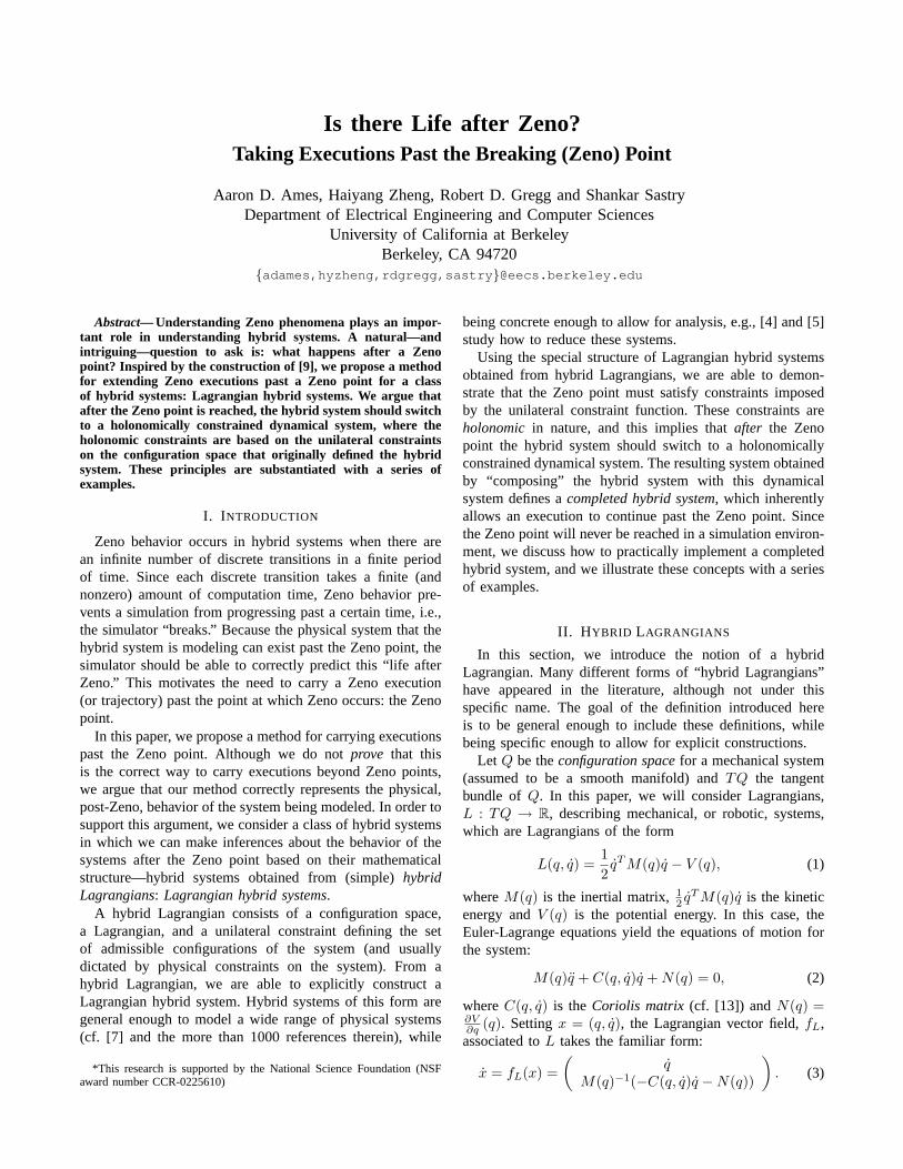
Fig. 1. Ball bouncing on a sinusoidal surface (left). Pendulum on a cart (middle). Spherical pendulum mounted on the ground (right).

This process of associating a dynamical system to a La-grangian will be mirrored in the setting of hybrid systems.First, we introduce the notion of a hybrid Lagrangian.

Definition 1: A simple hybrid Lagrangianis defined tobe a tuple

L = (Q, L, h),

where

• Q is the configuration space,• L : TQ → R is a hyperregular Lagrangian,• h : Q → R provides unilateral constraints on the

configuration space; we assume thath−1(0) is a smoothmanifold.

Example 1 (Ball): The first running example of this pa-per is a ball bouncing on a sinusoidal surface (cf. Fig. 1). Inthis case

B = (QB, LB, hB),

whereQB = R3, and forx = (x1, x2, x3),

LB(x, x) =12m‖x‖2 −mgx3.

Finally, we make the problem interesting by considering thesinusoidal constraint function

hB(x1, x2, x3) = x3 − sin(x2).

So, for this example, there are trivial dynamics and anontrivial constraint function.

Example 2 (Cart): Our second running example is a con-strained pendulum on a cart (cf. Fig. 1). This is a variationon the classical pendulum on a cart, where the pendulum isnot allowed to “pass through” the cart, i.e., the cart givesphysical constraints on the configuration space. In this case

C = (QC, LC, hC),

whereQC = S1 × R, q = (θ, x), and LC is the standardLagrangian associated to this system. Finally, the constraintthat the pendulum is not allowed to pass through the cart ismanifested in the constraint functionhC(θ, x) = cos(θ).

Example 3 (Pendulum):Our final running example is aspherical pendulum mounted on the ground (cf. Fig. 1). In

this case, the presence of the ground gives the physicalconstraints on the configuration space. That is, we define

P = (QP, LP, hP),

where QP = S2, q = (θ, ϕ), and LP is the standardLagrangian for this system. Finally, the constraint that thependulum is not allowed to pass through the ground ismanifested in the constraint functionhP(θ, ϕ) = cos(θ).

Definition 2: A simple hybrid systemis a tuple:

H = (D, f,G, R),

where

• D is a smooth manifold,• f is a vector field on that manifold,• G is an embedded submanifold ofG called theguard,• R is a smooth embeddingR : G → D called thereset

map.

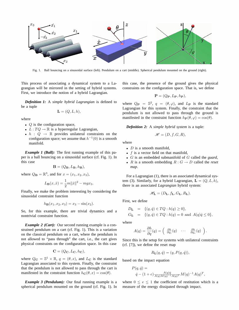
For a Lagrangian (1), there is an associated dynamical sys-tem (3). Similarly, for a hybrid Lagrangian,L = (Q,L, h),there is an associatedLagrangianhybrid system:

HL = (DL, fL, GL, RL).

First, we define

DL = {(q, q) ∈ TQ : h(q) ≥ 0},GL = {(q, q) ∈ TQ : h(q) = 0 and A(q)q ≤ 0},

where

A(q) =∂h

∂q(q) =

(∂h∂q1

(q) · · · ∂h∂qn

(q))

.

Since this is the setup for systems with unilateral constraints(cf. [7]), we define the reset map

RL(q, q) = (q, P (q, q)),

based on the impact equation

P (q, q) =

q − (1 + e) A(q)qA(q)M(q)−1A(q)T M(q)−1A(q)T ,

where 0 ≤ e ≤ 1 the coefficient of restitution which is ameasure of the energy dissipated through impact.

x ∈ GL

RL(x)

x = fL(x)

DL

Fig. 2. Lagrangian hybrid system obtained from a hybrid Lagrangian.

Finally, fL = fL is the Lagrangian vector field associatedto L. A graphical representation of the hybrid system is givenin Fig. 2.

Example 4: Utilizing the above construction, we can as-sociate to each of our running examples—the bouncing ball,the pendulum on a cart and the spherical pendulum—hybridsystemsHB, HC andHP, respectively.

Definition 3: An executionof H is a tuple

χH = (Λ, I,C),

where• Λ = {0, 1, 2, . . .} ⊆ N is a finite or infinite indexing

set,• I = {Ii}i∈Λ is a hybrid interval whereIi = [τi, τi+1]

if i, i+1 ∈ Λ andIN−1 = [τN−1, τN ] or [τN−1, τN ) or[τN−1,∞) if |Λ| = N , N finite, with τi, τi+1, τN ∈ Randτi ≤ τi+1,

• C = {ci}i∈Λ is a collection of solutions off , i.e.,ci(t) = f(ci(t)) for all i ∈ Λ,

such that the following conditions hold for everyi, i+1 ∈ Λ,

(i) ci(τi+1) ∈ G,(ii) R(ci(τi+1)) = ci+1(τi+1).

III. U NDERSTANDING ZENO BEHAVIOR

We begin this section by defining Zeno executions (cf.[1]-[6], [10], [11] and [15] for more on Zeno behavior).We then discuss two important classes of Zeno executions:chattering Zeno executionsand genuinely Zeno executions.In the context of Lagrangian hybrid systems obtained fromhybrid Lagrangians, we relate the coefficient of restitutionwith these two types of executions, and we give conditionsthat the Zeno point of a Zeno execution must satisfy in eithercase.

Definition 4: An executionχHL is Zeno if Λ = N and

limi→∞

τi =∞∑

i=0

(τi+1 − τi) = τ∞

for some finiteτ∞, termed theZeno time. If χHL is Zeno,then itsZeno pointis defined to be

x∞ = (q∞, q∞) = limi→∞

ci(τi) = limi→∞

(qi(τi), qi(τi)).

Here ci = (qi, qi) ∈ C, and the Zeno point is necessarilya single point because of the specific problem formulationconsidered in this paper.

A hybrid system is Zeno if it admits a Zeno execution,i.e., if there exists an executionχHL that is Zeno.

The definition of a Zeno execution results in two quali-tatively different types of Zeno behavior (cf. [3]); they aredefined as follows: a Zeno executionχHL is

Chattering Zeno: If there exists a finiteC suchthat τi+1 − τi = 0 for all i ≥ C.

Genuinely Zeno: If τi+1 − τi > 0 for all i ∈ N.

The difference between these is especially prevalent in theirdetection and elimination. Chattering Zeno executions resultfrom the existence of a switching surface on which the vectorfields “oppose” each other; for this reason they are easy todetect. Filippov solutions can be defined on these surfaces inorder to force the flow to “slide” along the switching surface(cf. [9]). Later in this paper we will generalize this techniqueto extend genuinely Zeno executions past the Zeno point.

Genuinely Zeno executions are much more complicatedin their behavior. There are very few methods currentlyavailable to detect the existence of genuinely Zeno execu-tions, namely [1] and [6]. Little has been done in the areaof eliminating these executions, although there have beensome results ([2] and [11]) for special classes of hybridsystems. This is the case because genuinely Zeno executionsare fundamentally global in nature, which prevents the useof local techniques in their analysis.

The hybrid systems considered in this paper display bothchattering and genuinely Zeno behavior; roughly speaking,the coefficient of restitution can be used to differentiatebetween these systems. Moreover, Zeno points must satisfycertain constraints based on the unilateral constraint function.That is, we make the following observations:

CZ: If HL has a chattering Zeno execution,χHL , then C = 1, i.e., τ∞ = τ1 − τ0 andx∞ = (q1(τ1), q1(τ1)) with h(q1(τ1)) = 0 andA(q1(τ1))q1(τ1) = 0.

GZ: If HL has a genuinely Zeno execution, then0 < e < 1. Moreover, if χHL is a genuinelyZeno execution, thenx∞ = (q∞, q∞) is a pointwith h(q∞) = 0, andA(q∞)q∞ = 0.

IV. GOING BEYOND ZENO

In this section, we propose a method for going beyondZeno points in the class of systems considered in this paper:Lagrangian hybrid systems. This method is supported bythe structure of the systems begin considered, although wedo not claim toprove that this is the right way to carryexecutions beyond Zeno points, or even that executionsshould necessarily be carried beyond Zeno points. We doclaim that if one wishes to carry an execution beyond a Zenopoint, and the system being considered is obtained from ahybrid Lagrangian, then this procedure gives a method by

which to do so. The authors are unaware of any similarresults in the literature.

We will assume that the hybrid system being consideredhere is Zeno, and thatχHL is a Zeno execution. Of course,for this procedure to be justifiable in a simulation framework,one must verifya priori that the system being consideredis Zeno. Although we will not explicitly derive conditionson when hybrid systems are Zeno, this is an active areaof research for the authors (cf. [1] and [6]). In the nextsection, we will indicate how to practically implement theresults given in this section. We begin by summarizingthe observations of the previous section by stating themconcisely.

Main Observation. If χHL is a Zeno executionof a Lagrangian hybrid systemHL, then theZeno pointx∞ = (q∞, q∞) is a point satisfyingh(q∞) = 0 and A(q∞)q∞ = 0.

This observation indicates how the system should behaveafter the Zeno point, i.e., it should satisfy a holonomicconstraint. This holonomic constraint forces the system toslide along surfaceh−1(0) = {q ∈ Q : h(q) = 0}. From this,we argue that after the Zeno point, the hybrid system shouldswitch to a holonomically constrained dynamical system.

Recall that for a holonomically constrained system de-scribed by a Lagrangian,L, of the form given in (1),the equations of motion for the holonomically constrainedsystem are obtained from the equations of motion for theunconstrained system (2); they are given by (cf. [13])

M(q)q + C(q, q)q + N(q) + A(q)T λ = 0,

where λ is the Lagrange multiplier, which in this case isgiven by

λ = (A(q)M(q)−1A(q)T )−1(

˙A(q)q

−A(q)M(q)−1(C(q, q)q + N(q))).

From the constrained equations of motion, forx = (q, q),we get the vector field

x = f∞L (x)

=(

qM(q)−1(−C(q, q)q −N(q)−A(q)T λ)

).

Note that thef∞L defines a vector field on the manifoldTQ|h−1(0), from which we obtain the dynamical system

D∞L = (TQ|h−1(0), f∞L ).

This, when coupled with the Main Observation, will beessential to understanding how to carry executions beyondZeno points.

We begin by considering the case whenHL is a chatteringZeno hybrid system; in this case, the idea of carryingexecutions past the Zeno point has been well-studied. In [9],it is argued that once the solution hits the “switching surface”(or, in our case, the guard), the solution should slide along theswitching surface. In terms of Zeno points, this implies that

x ∈ GL

RL(x)

x = fL(x)

DL

x = f∞L (x)

h(q) = 0

h(q) = 0 and A(q)q = 0

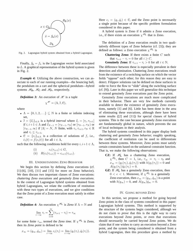
Fig. 3. A completed hybrid system:H L.

before the Zeno point the dynamics should be dictated byfL,while after the Zeno point the dynamics should be dictated byf∞L . We can generalize this construction to include genuinelyZeno Lagrangian hybrid systems.

Definition 5: If HL is a Lagrangian hybrid system, wedefine the correspondingcompleted hybrid system1 (or thecompletionof HL) as

H L :={

D∞L if h(q) = 0 and A(q)q = 0HL otherwise.

A completed hybrid system, as obtained from a La-grangian hybrid systemHL, can be seen in Fig. 3. Tomake the definition of the completed system somewhatmore transparent, some comments are in order. The MainObservation indicates that the only way for the transitionto be made from the hybrid systemHL to the dynamicalsystemD∞L is if a specific Zeno execution reaches its Zenopoint. Therefore, before the Zeno point, the Zeno systemsimply will be the hybrid systemHL, while after the Zenopoint, the completed system will be the dynamical systemD∞L . Since the dynamical system forces the system dynamicsto be constrained to the manifold defined byh−1(0), thisimplies that the completed system will slide along the guard(switching surface) after the Zeno point.

This can be understood further on the level of executions.We can define an execution of the completed hybrid systemH L by concatenating a Zeno execution ofHL with asolution to the dynamical systemD∞L .

Specifically, letχHL = (N, I,C) be a Zeno execution ofHL. We obtain an execution (or solution) of the completedhybrid systemH L by defining it to be

χH L = (N ∪ {∞}, I,C),

where

I = I ∪ {I∞ = [τ∞,∞)}, C = C ∪ {c∞},

with c∞(t) a solution tof∞L with initial condition the Zenopoint:

c∞(τ∞) = x∞ = (q∞, q∞).

In the next section, we will discuss how to simulate solutionsof completed systems.

1This terminology (and notation) is borrowed from topology, where ametric space can be completed to ensure that “limits exist.”

V. M ODELING AND SIMULATION

We discuss two practical issues when modeling and sim-ulating completed hybrid systems (see Fig. 3). These issuesare related to the transition from the left stateHL to the rightstateD∞L , and the corresponding initial conditions ofD∞L .The theoretical framework established in this paper allowsus to justifiably surmount the practical problems introducedin simulation.

The first simulation issue is derived from the unavoidablenumerical errors caused by finite representations of valuesin a computer and truncation errors introduced by practicalODE solvers, i.e., a simulator produces an approximateexecutionχHL to the executionχHL . Therefore, we can’tguarantee or expect a solution to reach the exact Zeno pointx∞ = (q∞, q∞). Moreover, in order to reach the Zeno point,an infinite number of computation steps have to be performed(in a finite amount of time). Therefore, instead of resolvinga solution that passes through the Zeno point exactly, wewill compute an approximation of the Zeno solution; theapproximated solution will pass through a neighborhood ofthe Zeno point, so we must modify the transition to thesystemD∞L accordingly. Before discussing the details of theconstruction of the approximate solution, we first address thesecond modeling issue.

The other concern is the reinitialization of the new con-strained systemD∞L . In other words, after the transitionto this system, we must give initial conditions for theconstrained system. Theoretically, the initial condition isthe Zeno point, but because in simulation we do not ac-tually reach the Zeno point, an initial condition must beestimated—one that satisfies the same conditions as a Zenopoint: h(q∞) = 0 andA(q∞)q∞ = 0.

The approximation to the completed hybrid systemH L,denoted byH

ε

L, is given by

Hε

L :={

D∞L if abs(h(q)) ≤ ε and abs(A(q)q) ≤ εHL otherwise.

When switching fromHL to D∞L via the approximated guardcondition, we use a map which resets the variables so thatthey satisfy the conditions of a Zeno point:h(q∞) = 0 andA(q∞)q∞ = 0. Specifically, for a point(q, q) satisfying theapproximate guard condition

abs(h(q)) ≤ ε and abs(A(q)q) ≤ ε,

we define a reset mapR∞ which sends(q, q) to an approx-imate Zeno point,(q∞, q∞) = R∞(q, q), satisfying

h(q∞) = 0 and A(q∞)q∞ = 0.

We now briefly discuss how to construct the mapR∞ forthe running examples in this paper. In all of these examples,the vector fields for the constrained dynamical systems areeasy to calculate.

Example 5: We begin by considering the ball. Note that

hB(x) = 0 ⇒ x3 = sin(x2),AB(x)x = 0 ⇒ x3 − cos(x2)x2 = 0.

In the above two equations, there are four variables—x2, x2, x3, and x3—involved but only two constraints,so we can’t resolve all of the variable values, i.e., wemust use part of the simulation results to obtain the initialconditions for the constrained systems. Finally, there areno extra constraints for the rest of the variables of thesystem—x1 and x1—and their initial conditions are simplythe simulation results. Therefore, if we use the simulationresults ofx2 and x2 to obtain the initial conditions for theconstrained system, the complete reset map is:

R∞B (x1, x2, x3, x1, x2, x3) =(x1, x2, sin(x2), x1, x2, cos(x2)x2).

For the other running examples, the calculations are thesame. The end result is that:

R∞C (θ, x, θ, x) = (sign(θ)π/2, x, 0, x),R∞P (θ, ϕ, θ, ϕ) = (π/2, ϕ, 0, ϕ).

We use HyVisual (cf. [8]) as the modeling and simulationtool. The semantics of a transition in this tool is thatwhenever its guard expression becomes true, the transition istaken immediately (cf. [12]). An event detection mechanismis deployed to ensure that a transition is taken close to thetime point when its guard expression becomes enabled. Thesesemantics are very important in ensuring that the simulationapproximates the exact Zeno solutions.

Next, we take a close look at the simulation results ofthe Ball example to illustrate how we approximate the exactZeno solution.

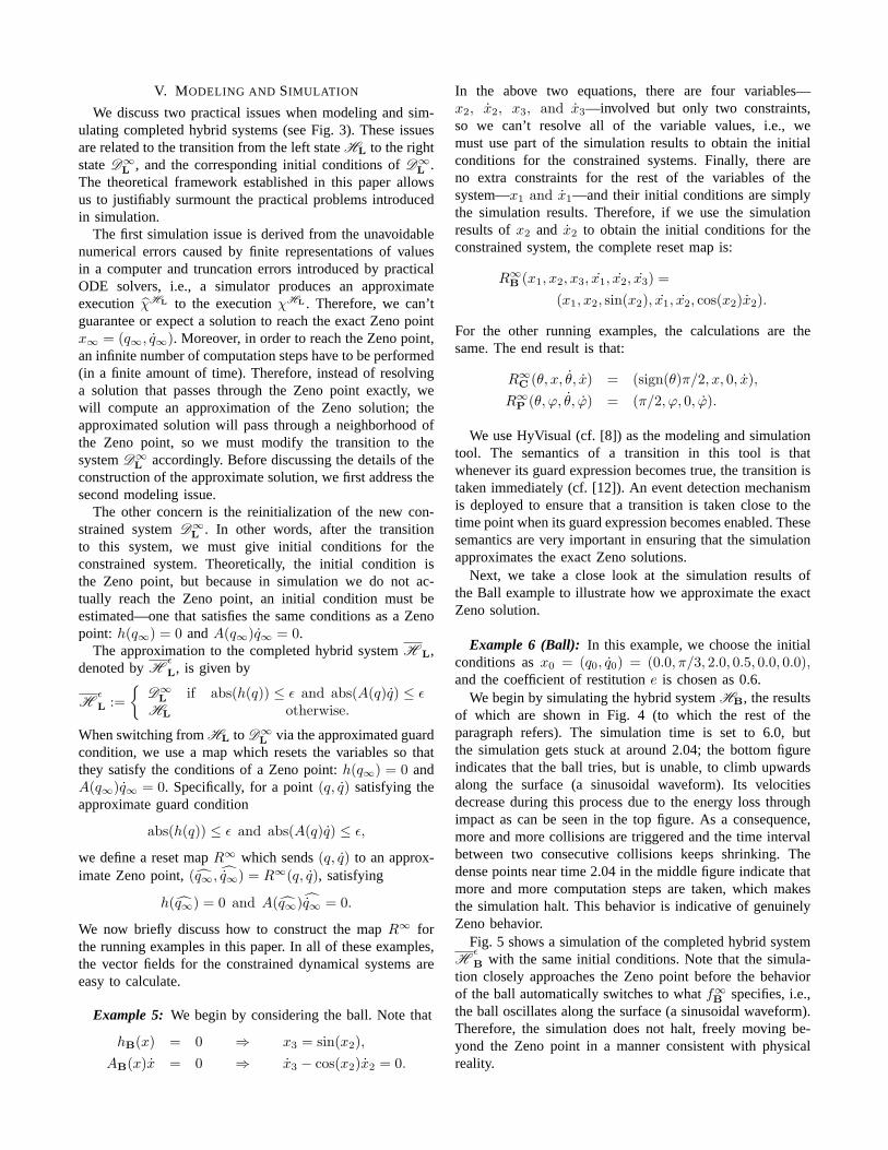
Example 6 (Ball): In this example, we choose the initialconditions asx0 = (q0, q0) = (0.0, π/3, 2.0, 0.5, 0.0, 0.0),and the coefficient of restitutione is chosen as 0.6.

We begin by simulating the hybrid systemHB, the resultsof which are shown in Fig. 4 (to which the rest of theparagraph refers). The simulation time is set to 6.0, butthe simulation gets stuck at around 2.04; the bottom figureindicates that the ball tries, but is unable, to climb upwardsalong the surface (a sinusoidal waveform). Its velocitiesdecrease during this process due to the energy loss throughimpact as can be seen in the top figure. As a consequence,more and more collisions are triggered and the time intervalbetween two consecutive collisions keeps shrinking. Thedense points near time 2.04 in the middle figure indicate thatmore and more computation steps are taken, which makesthe simulation halt. This behavior is indicative of genuinelyZeno behavior.

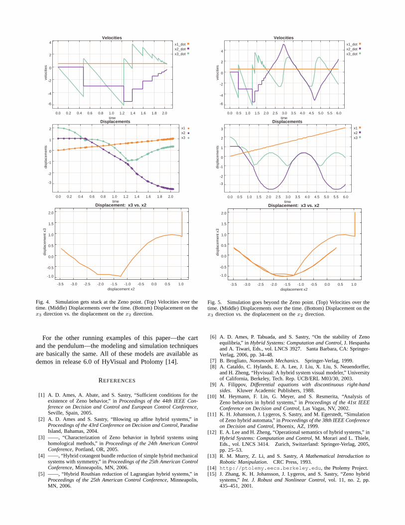
Fig. 5 shows a simulation of the completed hybrid systemH

ε

B with the same initial conditions. Note that the simula-tion closely approaches the Zeno point before the behaviorof the ball automatically switches to whatf∞B specifies, i.e.,the ball oscillates along the surface (a sinusoidal waveform).Therefore, the simulation does not halt, freely moving be-yond the Zeno point in a manner consistent with physicalreality.

x1_dotx2_dotx3_dot

-6

-4

-2

0

2

4

0.0 0.2 0.4 0.6 0.8 1.0 1.2 1.4 1.6 1.8 2.0

Velocities

time

velo

citie

s

x1x2x3

-3

-2

-1

0

1

2

0.0 0.2 0.4 0.6 0.8 1.0 1.2 1.4 1.6 1.8 2.0

Displacements

time

disp

lace

men

ts

-1.0

-0.5

0.0

0.5

1.0

1.5

2.0

-3.5 -3.0 -2.5 -2.0 -1.5 -1.0 -0.5 0.0 0.5 1.0

Displacement: x3 vs. x2

displacement x2

disp

lace

men

t x3

Fig. 4. Simulation gets stuck at the Zeno point. (Top) Velocities over thetime. (Middle) Displacements over the time. (Bottom) Displacement on thex3 direction vs. the displacement on thex2 direction.

For the other running examples of this paper—the cartand the pendulum—the modeling and simulation techniquesare basically the same. All of these models are available asdemos in release 6.0 of HyVisual and Ptolomy [14].

REFERENCES

[1] A. D. Ames, A. Abate, and S. Sastry, “Sufficient conditions for theexistence of Zeno behavior,” inProceedings of the 44th IEEE Con-ference on Decision and Control and European Control Conference,Seville, Spain, 2005.

[2] A. D. Ames and S. Sastry, “Blowing up affine hybrid systems,” inProceedings of the 43rd Conference on Decision and Control, ParadiseIsland, Bahamas, 2004.

[3] ——, “Characterization of Zeno behavior in hybrid systems usinghomological methods,” inProceedings of the 24th American ControlConference, Portland, OR, 2005.

[4] ——, “Hybrid cotangent bundle reduction of simple hybrid mechanicalsystems with symmetry,” inProceedings of the 25th American ControlConference, Minneapolis, MN, 2006.

[5] ——, “Hybrid Routhian reduction of Lagrangian hybrid systems,” inProceedings of the 25th American Control Conference, Minneapolis,MN, 2006.

x1_dotx2_dotx3_dot

-6

-4

-2

0

2

4

0.0 0.5 1.0 1.5 2.0 2.5 3.0 3.5 4.0 4.5 5.0 5.5 6.0

Velocities

time

velo

citie

s

x1x2x3

-3

-2

-1

0

1

2

3

0.0 0.5 1.0 1.5 2.0 2.5 3.0 3.5 4.0 4.5 5.0 5.5 6.0

Displacements

time

disp

lace

men

ts

-1.0

-0.5

0.0

0.5

1.0

1.5

2.0

-3.5 -3.0 -2.5 -2.0 -1.5 -1.0 -0.5 0.0 0.5 1.0

Displacement: x3 vs. x2

displacement x2

disp

lace

men

t x3

Fig. 5. Simulation goes beyond the Zeno point. (Top) Velocities over thetime. (Middle) Displacements over the time. (Bottom) Displacement on thex3 direction vs. the displacement on thex2 direction.

[6] A. D. Ames, P. Tabuada, and S. Sastry, “On the stability of Zenoequilibria,” in Hybrid Systems: Computation and Control, J. Hespanhaand A. Tiwari, Eds., vol. LNCS 3927. Santa Barbara, CA: Springer-Verlag, 2006, pp. 34–48.

[7] B. Brogliato, Nonsmooth Mechanics. Springer-Verlag, 1999.[8] A. Cataldo, C. Hylands, E. A. Lee, J. Liu, X. Liu, S. Neuendorffer,

and H. Zheng, “Hyvisual: A hybrid system visual modeler,” Universityof California, Berkeley, Tech. Rep. UCB/ERL M03/30, 2003.

[9] A. Filippov, Differential equations with discontinuous right-handsides. Kluwer Academic Publishers, 1988.

[10] M. Heymann, F. Lin, G. Meyer, and S. Resmerita, “Analysis ofZeno behaviors in hybrid systems,” inProceedings of the 41st IEEEConference on Decision and Control, Las Vagas, NV, 2002.

[11] K. H. Johansson, J. Lygeros, S. Sastry, and M. Egerstedt, “Simulationof Zeno hybrid automata,” inProceedings of the 38th IEEE Conferenceon Decision and Control, Phoenix, AZ, 1999.

[12] E. A. Lee and H. Zheng, “Operational semantics of hybrid systems,” inHybrid Systems: Computation and Control, M. Morari and L. Thiele,Eds., vol. LNCS 3414. Zurich, Switzerland: Springer-Verlag, 2005,pp. 25–53.

[13] R. M. Murry, Z. Li, and S. Sastry,A Mathematical Introduction toRobotic Manipulation. CRC Press, 1993.

[14] http://ptolemy.eecs.berkeley.edu , the Ptolemy Project.[15] J. Zhang, K. H. Johansson, J. Lygeros, and S. Sastry, “Zeno hybrid

systems,”Int. J. Robust and Nonlinear Control, vol. 11, no. 2, pp.435–451, 2001.