is prof aba power of - university of wisconsin–eau claire of proofs from the...hello prospective...

Hello Prospective Students of aBa’s Math 395 course on the Beauty of Math,

This 66 page PDF contains the 1pg course outline and an excerpt from the text

Proofs from THE BOOK. It is chapter one on the topic of number theory. This is

one of 5 areas of math which we will explore in Part 1 of the course dealing with

BEAUTIFUL PROOFS. You ABSOLUTELY need to have taken (even concurrently this

Fall 2014) at least ONE of the following proof-writing courses: 314, 324, or 425.

By the way, there have been selective blank pages placed into the PDF to preserve

the front and back pages as they appear in the book. So print this pdf DOUBLE-

SIDED starting with pg.1 or pg.3 (if you want to start with the “cover” of the book

– well, I made this cover, it’s not the official cover of the book).

Part 2 of the course will be on combinatorics of permutations. There is a lot of

beauty here too and this is part of my research area, so this part of the course will

give you a flavor of what doing research with me might entail. Specifically in my

research with a future student, I would like to extend the topics in part 2 to the

world of imprimitive complex reflection groups (think of permutation matrices

where the nonzero entries are rth roots of unity). This group is a generalization of

the symmetric group which you have seen in Math 312 and definitely in Math 425

(and in its permutation matrix form in Math 324). I will brush you up on this if it is

foggy or missing completely from your memory.

Shalom,

aBa

Is Prof aBa “Power of brANDing” this course

with me, the cat?

“Beautiful Proofs in Mathematics and an Exploration of the Combinatorics of Permutations”

Prof aBa’s Math 395 Directed Studies Course – Fall 2014 (1 credit course meeting 1 hour per week – time & place TBD)

GOAL OF COURSE: There are two. First, we explore the most BEAUTIFUL proofs in

mathematics. And I mean that! Second, we focus on combinatorial objects called permutations and study various combinatorial properties of these objects.

TEXTBOOKS: (I will provide excerpts of these for you as needed) Proofs from THE BOOK (4th Edition) by Martin Aigner and Günther M. Ziegler (2010) Combinatorics of Permutations by Miklos Bóna (2004) The Symmetric Group (2nd Edition) by Bruce Sagan (2001)

FORMAT OF PART 1 OF THE COURSE: Since this is a directed studies course, we will all take part in teaching it. The plan for the “Beauty of Mathematics” part of the course is for each of us to take turns presenting proofs from the book called Proofs from THE BOOK. This part will be REALLY fun because there are quite a variety of topics presented and EVERYTHING is beautiful. We will be learning some of the most fundamental results in areas of math from number theory, geometry, analysis, combinatorics, and graph theory.

FORMAT OF PART 2 OF THE COURSE: This will start out with me lecturing on permutations like in a standard lecture class. Then students present material. Time-permitting, we will explore possible directions of research that we can do next semester, next summer, next year, or whenever!

CAVEAT!!!: There being two parts to this course does NOT mean that Part 1 takes

half the semester and Part 2 is the other half. If we are having LOADS of fun with Part 1, then we can just continue presenting the most beautiful proofs to one another. I can always teach Part 2 next semester, if that is the case! And if after the 1st two weeks or so, everyone is bored with beautiful proofs, then we can move on to Part 2.

Paul Erdős liked to talk about THE BOOK, in which God maintains the perfect proofs for mathematical theorems, following the dictum of G.H. Hardy that there is no permanent place for ugly mathematics.

“You do not have to believe in God but, as a mathematician, you should believe in the book.” -Paul Erdős

Martin AignerGünter M. Ziegler

Proofs fromTHE BOOKFourth Edition

Including Illustrations by Karl H. Hofmann

123

Prof. Dr. Martin AignerFB Mathematik und InformatikFreie Universität BerlinArnimallee 314195 [email protected]

Prof. Günter M. ZieglerInstitut für Mathematik, MA 6-2Technische Universität BerlinStraße des 17. Juni 13610623 [email protected]

ISBN 978-3-642-00855-9 e-ISBN 978-3-642-00856-6DOI 10.1007/978-3-642-00856-6Springer Heidelberg Dordrecht London New York

c© Springer-Verlag Berlin Heidelberg 2010This work is subject to copyright. All rights are reserved, whether the whole or part of thematerial is concerned, specif ically the rights of translation, reprinting, reuse of illustrations,recitation, broadcasting, reproduction on microfilm or in any other way, and storage in databanks. Duplication of this publication or parts thereof is permitted only under the provisions ofthe German Copyright Law of September 9, 1965, in its current version, and permission for usemust always be obtained from Springer. Violations are liable to prosecution under the GermanCopyright Law.The use of general descriptive names, registered names, trademarks, etc. in this publicationdoes not imply, even in the absence of a specif ic statement, that such names are exempt fromthe relevant protective laws and regulations and therefore free for general use.

Cover design: ,

Printed on acid-free paper

Springer is part of Springer Science+Business Media (www.springer.com)

deblik Berlin

Preface

Paul Erdos

Paul Erdos liked to talk about The Book, in which God maintains the perfectproofs for mathematical theorems, following the dictum of G. H. Hardy thatthere is no permanent place for ugly mathematics. Erdos also said that youneed not believe in God but, as a mathematician, you should believe inThe Book. A few years ago, we suggested to him to write up a first (andvery modest) approximation to The Book. He was enthusiastic about theidea and, characteristically, went to work immediately, filling page afterpage with his suggestions. Our book was supposed to appear in March1998 as a present to Erdos’ 85th birthday. With Paul’s unfortunate deathin the summer of 1996, he is not listed as a co-author. Instead this book isdedicated to his memory.

“The Book”

We have no definition or characterization of what constitutes a proof fromThe Book: all we offer here is the examples that we have selected, hop-ing that our readers will share our enthusiasm about brilliant ideas, cleverinsights and wonderful observations. We also hope that our readers willenjoy this despite the imperfections of our exposition. The selection is to agreat extent influenced by Paul Erdos himself. A large number of the topicswere suggested by him, and many of the proofs trace directly back to him,or were initiated by his supreme insight in asking the right question or inmaking the right conjecture. So to a large extent this book reflects the viewsof Paul Erdos as to what should be considered a proof from The Book.

A limiting factor for our selection of topics was that everything in this bookis supposed to be accessible to readers whose backgrounds include onlya modest amount of technique from undergraduate mathematics. A littlelinear algebra, some basic analysis and number theory, and a healthy dollopof elementary concepts and reasonings from discrete mathematics shouldbe sufficient to understand and enjoy everything in this book.

We are extremely grateful to the many people who helped and supportedus with this project — among them the students of a seminar where wediscussed a preliminary version, to Benno Artmann, Stephan Brandt, StefanFelsner, Eli Goodman, Torsten Heldmann, and Hans Mielke. We thankMargrit Barrett, Christian Bressler, Ewgenij Gawrilow, Michael Joswig,Elke Pose, and Jörg Rambau for their technical help in composing thisbook. We are in great debt to Tom Trotter who read the manuscript fromfirst to last page, to Karl H. Hofmann for his wonderful drawings, andmost of all to the late great Paul Erdos himself.

Berlin, March 1998 Martin Aigner · Günter M. Ziegler

VI

Preface to the Fourth Edition

When we started this project almost fifteen years ago we could not possiblyimagine what a wonderful and lasting response our book about The Bookwould have, with all the warm letters, interesting comments, new editions,and as of now thirteen translations. It is no exaggeration to say that it hasbecome a part of our lives.

In addition to numerous improvements, partly suggested by our readers, thepresent fourth edition contains five new chapters: Two classics, the law ofquadratic reciprocity and the fundamental theorem of algebra, two chapterson tiling problems and their intriguing solutions, and a highlight in graphtheory, the chromatic number of Kneser graphs.

We thank everyone who helped and encouraged us over all these years: Forthe second edition this included Stephan Brandt, Christian Elsholtz, JürgenElstrodt, Daniel Grieser, Roger Heath-Brown, Lee L. Keener, ChristianLebœuf, Hanfried Lenz, Nicolas Puech, John Scholes, Bernulf Weißbach,and many others. The third edition benefitted especially from input byDavid Bevan, Anders Björner, Dietrich Braess, John Cosgrave, HubertKalf, Günter Pickert, Alistair Sinclair, and Herb Wilf. For the present edi-tion, we are particularly grateful to contributions by France Dacar, OliverDeiser, Anton Dochtermann, Michael Harbeck, Stefan Hougardy, HendrikW. Lenstra, Günter Rote, Moritz Schmitt, and Carsten Schultz. Moreover,we thank Ruth Allewelt at Springer in Heidelberg as well as ChristophEyrich, Torsten Heldmann, and Elke Pose in Berlin for their help and sup-port throughout these years. And finally, this book would certainly not lookthe same without the original design suggested by Karl-Friedrich Koch, andthe superb new drawings provided for each edition by Karl H. Hofmann.

Berlin, July 2009 Martin Aigner · Günter M. Ziegler

Table of Contents

Number Theory 1

1. Six proofs of the infinity of primes . . . . . . . . . . . . . . . . . . . . . . . . . . . . . . 3

2. Bertrand’s postulate . . . . . . . . . . . . . . . . . . . . . . . . . . . . . . . . . . . . . . . . . . . .7

3. Binomial coefficients are (almost) never powers . . . . . . . . . . . . . . . . . 13

4. Representing numbers as sums of two squares . . . . . . . . . . . . . . . . . . . 17

5. The law of quadratic reciprocity . . . . . . . . . . . . . . . . . . . . . . . . . . . . . . . 23

6. Every finite division ring is a field . . . . . . . . . . . . . . . . . . . . . . . . . . . . . . 31

7. Some irrational numbers . . . . . . . . . . . . . . . . . . . . . . . . . . . . . . . . . . . . . . 35

8. Three times π2/6 . . . . . . . . . . . . . . . . . . . . . . . . . . . . . . . . . . . . . . . . . . . . . 43

Geometry 51

9. Hilbert’s third problem: decomposing polyhedra . . . . . . . . . . . . . . . . .53

10. Lines in the plane and decompositions of graphs . . . . . . . . . . . . . . . . .63

11. The slope problem . . . . . . . . . . . . . . . . . . . . . . . . . . . . . . . . . . . . . . . . . . . .69

12. Three applications of Euler’s formula . . . . . . . . . . . . . . . . . . . . . . . . . . 75

13. Cauchy’s rigidity theorem . . . . . . . . . . . . . . . . . . . . . . . . . . . . . . . . . . . . . 81

14. Touching simplices . . . . . . . . . . . . . . . . . . . . . . . . . . . . . . . . . . . . . . . . . . . 85

15. Every large point set has an obtuse angle . . . . . . . . . . . . . . . . . . . . . . . 89

16. Borsuk’s conjecture . . . . . . . . . . . . . . . . . . . . . . . . . . . . . . . . . . . . . . . . . . 95

Analysis 101

17. Sets, functions, and the continuum hypothesis . . . . . . . . . . . . . . . . . . 103

18. In praise of inequalities . . . . . . . . . . . . . . . . . . . . . . . . . . . . . . . . . . . . . . 119

19. The fundamental theorem of algebra . . . . . . . . . . . . . . . . . . . . . . . . . . 127

20. One square and an odd number of triangles . . . . . . . . . . . . . . . . . . . . 131

VIII Table of Contents

21. A theorem of Pólya on polynomials . . . . . . . . . . . . . . . . . . . . . . . . . . . 139

22. On a lemma of Littlewood and Offord . . . . . . . . . . . . . . . . . . . . . . . . . 145

23. Cotangent and the Herglotz trick . . . . . . . . . . . . . . . . . . . . . . . . . . . . . . 149

24. Buffon’s needle problem . . . . . . . . . . . . . . . . . . . . . . . . . . . . . . . . . . . . . 155

Combinatorics 159

25. Pigeon-hole and double counting . . . . . . . . . . . . . . . . . . . . . . . . . . . . . 161

26. Tiling rectangles . . . . . . . . . . . . . . . . . . . . . . . . . . . . . . . . . . . . . . . . . . . . 173

27. Three famous theorems on finite sets . . . . . . . . . . . . . . . . . . . . . . . . . . 179

28. Shuffling cards . . . . . . . . . . . . . . . . . . . . . . . . . . . . . . . . . . . . . . . . . . . . . . 185

29. Lattice paths and determinants . . . . . . . . . . . . . . . . . . . . . . . . . . . . . . . . 195

30. Cayley’s formula for the number of trees . . . . . . . . . . . . . . . . . . . . . . 201

31. Identities versus bijections . . . . . . . . . . . . . . . . . . . . . . . . . . . . . . . . . . . 207

32. Completing Latin squares . . . . . . . . . . . . . . . . . . . . . . . . . . . . . . . . . . . . 213

Graph Theory 219

33. The Dinitz problem . . . . . . . . . . . . . . . . . . . . . . . . . . . . . . . . . . . . . . . . . .221

34. Five-coloring plane graphs . . . . . . . . . . . . . . . . . . . . . . . . . . . . . . . . . . . 227

35. How to guard a museum . . . . . . . . . . . . . . . . . . . . . . . . . . . . . . . . . . . . . 231

36. Turán’s graph theorem . . . . . . . . . . . . . . . . . . . . . . . . . . . . . . . . . . . . . . . 235

37. Communicating without errors . . . . . . . . . . . . . . . . . . . . . . . . . . . . . . . 241

38. The chromatic number of Kneser graphs . . . . . . . . . . . . . . . . . . . . . . . 251

39. Of friends and politicians . . . . . . . . . . . . . . . . . . . . . . . . . . . . . . . . . . . . 257

40. Probability makes counting (sometimes) easy . . . . . . . . . . . . . . . . . . 261

About the Illustrations 270

Index 271

Number Theory

1Six proofsof the infinity of primes 3

2Bertrand’s postulate 7

3Binomial coefficientsare (almost) never powers 13

4Representing numbersas sums of two squares 17

5The law ofquadratic reciprocity 23

6Every finite division ringis a field 31

7Some irrational numbers 35

8Three times π2/6 43

“Irrationality and π”

Six proofs

of the infinity of primes

Chapter 1

It is only natural that we start these notes with probably the oldest BookProof, usually attributed to Euclid (Elements IX, 20). It shows that thesequence of primes does not end.

� Euclid’s Proof. For any finite set {p1, . . . , pr} of primes, considerthe number n = p1p2 · · · pr + 1. This n has a prime divisor p. But p isnot one of the pi: otherwise p would be a divisor of n and of the productp1p2 · · · pr, and thus also of the difference n − p1p2 · · · pr = 1, which isimpossible. So a finite set {p1, . . . , pr} cannot be the collection of all primenumbers. �

Before we continue let us fix some notation. N = {1, 2, 3, . . .} is the setof natural numbers, Z = {. . . ,−2,−1, 0, 1, 2, . . .} the set of integers, andP = {2, 3, 5, 7, . . .} the set of primes.

In the following, we will exhibit various other proofs (out of a much longerlist) which we hope the reader will like as much as we do. Although theyuse different view-points, the following basic idea is common to all of them:The natural numbers grow beyond all bounds, and every natural numbern ≥ 2 has a prime divisor. These two facts taken together force P to beinfinite. The next proof is due to Christian Goldbach (from a letter to Leon-hard Euler 1730), the third proof is apparently folklore, the fourth one isby Euler himself, the fifth proof was proposed by Harry Fürstenberg, whilethe last proof is due to Paul Erdos.

� Second Proof. Let us first look at the Fermat numbers Fn = 22n

+1 forn = 0, 1, 2, . . .. We will show that any two Fermat numbers are relativelyprime; hence there must be infinitely many primes. To this end, we verifythe recursion n−1∏

k=0

Fk = Fn − 2 (n ≥ 1),

from which our assertion follows immediately. Indeed, if m is a divisor of,

F0 = 3F1 = 5F2 = 17F3 = 257F4 = 65537F5 = 641 · 6700417

The first few Fermat numbers

say, Fk and Fn (k < n), then m divides 2, and hence m = 1 or 2. Butm = 2 is impossible since all Fermat numbers are odd.

To prove the recursion we use induction on n. For n = 1 we have F0 = 3and F1 − 2 = 3. With induction we now conclude

n∏

k=0

Fk =( n−1∏

k=0

Fk

)Fn = (Fn − 2)Fn =

= (22n − 1)(22n

+ 1) = 22n+1 − 1 = Fn+1 − 2. �

4 Six proofs of the infinity of primes

� Third Proof. Suppose P is finite and p is the largest prime. We considerthe so-called Mersenne number 2p − 1 and show that any prime factor qof 2p− 1 is bigger than p, which will yield the desired conclusion. Let q bea prime dividing 2p − 1, so we have 2p ≡ 1 (mod q). Since p is prime, this

Lagrange’s Theorem

If G is a finite (multiplicative) groupand U is a subgroup, then |U |divides |G|.� Proof. Consider the binary rela-tion

a ∼ b : ⇐⇒ ba−1 ∈ U.

It follows from the group axiomsthat ∼ is an equivalence relation.The equivalence class containing anelement a is precisely the coset

Ua = {xa : x ∈ U}.

Since clearly |Ua| = |U |, we findthat G decomposes into equivalenceclasses, all of size |U |, and hencethat |U | divides |G|. �

In the special case when U is a cyclicsubgroup {a, a2, . . . , am} we findthat m (the smallest positive inte-ger such that am = 1, called theorder of a) divides the size |G| ofthe group.

means that the element 2 has order p in the multiplicative group Zq\{0} ofthe field Zq . This group has q − 1 elements. By Lagrange’s theorem (seethe box) we know that the order of every element divides the size of thegroup, that is, we have p | q − 1, and hence p < q. �

Now let us look at a proof that uses elementary calculus.

� Fourth Proof. Let π(x) := #{p ≤ x : p ∈ P} be the number of primesthat are less than or equal to the real number x. We number the primesP = {p1, p2, p3, . . .} in increasing order. Consider the natural logarithmlog x, defined as log x =

∫ x

11t dt.

21

1

n n+1

Steps above the function f(t) = 1t

Now we compare the area below the graph of f(t) = 1t with an upper step

function. (See also the appendix on page 10 for this method.) Thus forn ≤ x < n+ 1 we have

log x ≤ 1 +1

2+

1

3+ . . .+

1

n− 1+

1

n

≤∑ 1

m, where the sum extends over allm ∈ N which have

only prime divisors p ≤ x.

Since every suchm can be written in a unique way as a product of the form∏p≤x

pkp , we see that the last sum is equal to

∏

p∈Pp≤x

(∑

k≥0

1

pk

).

The inner sum is a geometric series with ratio 1p , hence

log x ≤∏

p∈Pp≤x

1

1− 1p

=∏

p∈Pp≤x

p

p− 1=

π(x)∏

k=1

pk

pk − 1.

Now clearly pk ≥ k + 1, and thus

pk

pk − 1= 1 +

1

pk − 1≤ 1 +

1

k=

k + 1

k,

and therefore

log x ≤π(x)∏

k=1

k + 1

k= π(x) + 1.

Everybody knows that log x is not bounded, so we conclude that π(x) isunbounded as well, and so there are infinitely many primes. �

Six proofs of the infinity of primes 5

� Fifth Proof. After analysis it’s topology now! Consider the followingcurious topology on the set Z of integers. For a, b ∈ Z, b > 0, we set

Na,b = {a+ nb : n ∈ Z}.

Each set Na,b is a two-way infinite arithmetic progression. Now call a setO ⊆ Z open if either O is empty, or if to every a ∈ O there exists someb > 0 with Na,b ⊆ O. Clearly, the union of open sets is open again. IfO1, O2 are open, and a ∈ O1 ∩ O2 with Na,b1 ⊆ O1 and Na,b2 ⊆ O2,then a ∈ Na,b1b2 ⊆ O1 ∩ O2. So we conclude that any finite intersectionof open sets is again open. So, this family of open sets induces a bona fidetopology on Z.

Let us note two facts:

(A) Any nonempty open set is infinite.

(B) Any set Na,b is closed as well.

Indeed, the first fact follows from the definition. For the second we observe

Na,b = Z \b−1⋃

i=1

Na+i,b,

which proves that Na,b is the complement of an open set and hence closed.

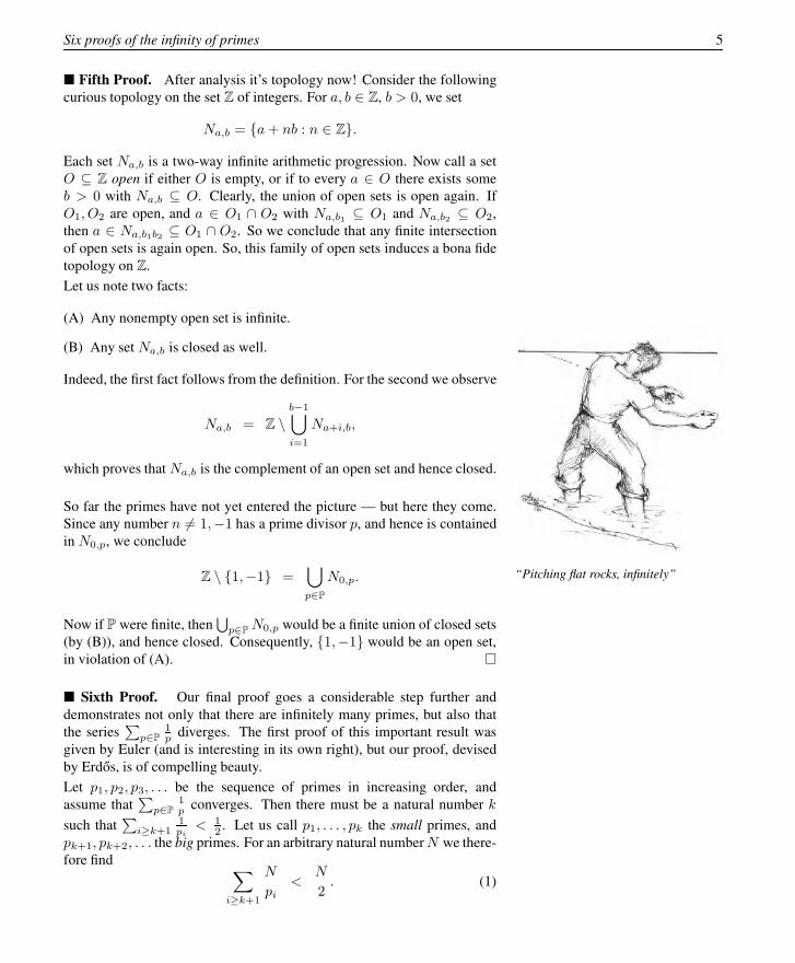
“Pitching flat rocks, infinitely”

So far the primes have not yet entered the picture — but here they come.Since any number n 6= 1,−1 has a prime divisor p, and hence is containedin N0,p, we conclude

Z \ {1,−1} =⋃

p∈P

N0,p.

Now if P were finite, then⋃

p∈P N0,p would be a finite union of closed sets(by (B)), and hence closed. Consequently, {1,−1} would be an open set,in violation of (A). �

� Sixth Proof. Our final proof goes a considerable step further anddemonstrates not only that there are infinitely many primes, but also thatthe series

∑p∈P

1p diverges. The first proof of this important result was

given by Euler (and is interesting in its own right), but our proof, devisedby Erdos, is of compelling beauty.

Let p1, p2, p3, . . . be the sequence of primes in increasing order, andassume that

∑p∈P

1p converges. Then there must be a natural number k

such that∑

i≥k+11pi

< 12 . Let us call p1, . . . , pk the small primes, and

pk+1, pk+2, . . . the big primes. For an arbitrary natural numberN we there-fore find ∑

i≥k+1

N

pi<

N

2. (1)

6 Six proofs of the infinity of primes

Let Nb be the number of positive integers n ≤ N which are divisible by atleast one big prime, and Ns the number of positive integers n ≤ N whichhave only small prime divisors. We are going to show that for a suitable N

Nb +Ns < N,

which will be our desired contradiction, since by definitionNb +Ns wouldhave to be equal to N .

To estimate Nb note that ⌊Npi⌋ counts the positive integers n ≤ N which

are multiples of pi. Hence by (1) we obtain

Nb ≤∑

i≥k+1

⌊Npi

⌋<

N

2. (2)

Let us now look at Ns. We write every n ≤ N which has only small primedivisors in the form n = anb

2n, where an is the square-free part. Every an

is thus a product of different small primes, and we conclude that there areprecisely 2k different square-free parts. Furthermore, as bn ≤

√n ≤√N ,

we find that there are at most√N different square parts, and so

Ns ≤ 2k√N.

Since (2) holds for anyN , it remains to find a numberN with 2k√N ≤ N

2

or 2k+1 ≤√N , and for this N = 22k+2 will do. �

References

[1] B. ARTMANN: Euclid — The Creation of Mathematics, Springer-Verlag, NewYork 1999.

[2] P. ERDOS: Über die ReiheP

1p

, Mathematica, Zutphen B 7 (1938), 1-2.

[3] L. EULER: Introductio in Analysin Infinitorum, Tomus Primus, Lausanne1748; Opera Omnia, Ser. 1, Vol. 8.

[4] H. FÜRSTENBERG: On the infinitude of primes, Amer. Math. Monthly 62

(1955), 353.

Bertrand’s postulate Chapter 2

Joseph Bertrand

We have seen that the sequence of prime numbers 2, 3, 5, 7, . . . is infinite.To see that the size of its gaps is not bounded, let N := 2 · 3 · 5 · · · p denotethe product of all prime numbers that are smaller than k + 2, and note thatnone of the k numbers

N + 2, N + 3, N + 4, . . . , N + k,N + (k + 1)

is prime, since for 2 ≤ i ≤ k + 1 we know that i has a prime factor that issmaller than k + 2, and this factor also divides N , and hence also N + i.With this recipe, we find, for example, for k = 10 that none of the tennumbers

2312, 2313, 2314, . . . , 2321

is prime.

But there are also upper bounds for the gaps in the sequence of prime num-bers. A famous bound states that “the gap to the next prime cannot be largerthan the number we start our search at.” This is known as Bertrand’s pos-tulate, since it was conjectured and verified empirically for n < 3 000 000by Joseph Bertrand. It was first proved for all n by Pafnuty Chebyshev in1850. A much simpler proof was given by the Indian genius Ramanujan.Our Book Proof is by Paul Erdos: it is taken from Erdos’ first publishedpaper, which appeared in 1932, when Erdos was 19.

Bertrand’s postulate.

For every n ≥ 1, there is some prime number p with n < p ≤ 2n.

� Proof. We will estimate the size of the binomial coefficient(2nn

)care-

fully enough to see that if it didn’t have any prime factors in the rangen < p ≤ 2n, then it would be “too small.” Our argument is in five steps.

(1) We first prove Bertrand’s postulate for n < 4000. For this one does notneed to check 4000 cases: it suffices (this is “Landau’s trick”) to check that

2, 3, 5, 7, 13, 23, 43, 83, 163, 317, 631, 1259, 2503, 4001

is a sequence of prime numbers, where each is smaller than twice the previ-ous one. Hence every interval {y : n < y ≤ 2n}, with n ≤ 4000, containsone of these 14 primes.

8 Bertrand’s postulate

(2) Next we prove that∏

p≤x

p ≤ 4x−1 for all real x ≥ 2, (1)

where our notation — here and in the following — is meant to imply thatthe product is taken over all prime numbers p ≤ x. The proof that wepresent for this fact uses induction on the number of these primes. It isnot from Erdos’ original paper, but it is also due to Erdos (see the margin),and it is a true Book Proof. First we note that if q is the largest prime withq ≤ x, then

∏

p≤x

p =∏

p≤q

p and 4q−1 ≤ 4x−1.

Thus it suffices to check (1) for the case where x = q is a prime number. Forq = 2 we get “2 ≤ 4,” so we proceed to consider odd primes q = 2m+ 1.(Here we may assume, by induction, that (1) is valid for all integers x inthe set {2, 3, . . . , 2m}.) For q = 2m+ 1 we split the product and compute

∏

p≤2m+1

p =∏

p≤m+1

p ·∏

m+1<p≤2m+1

p ≤ 4m

(2m+ 1

m

)≤ 4m22m = 42m.

All the pieces of this “one-line computation” are easy to see. In fact,∏

p≤m+1

p ≤ 4m

holds by induction. The inequality

∏

m+1<p≤2m+1

p ≤(

2m+ 1

m

)

follows from the observation that(2m+1

m

)= (2m+1)!

m!(m+1)! is an integer, wherethe primes that we consider all are factors of the numerator (2m+ 1)!, butnot of the denominatorm!(m+ 1)!. Finally

(2m+ 1

m

)≤ 22m

holds since (2m+ 1

m

)and

(2m+ 1

m+ 1

)

Legendre’s theorem

The number n! contains the primefactor p exactly

X

k≥1

j n

pk

k

times.

� Proof. Exactly¨

np

˝

of the factorsof n! = 1 · 2 · 3 · · ·n are divisible byp, which accounts for

¨

np

˝

p-factors.Next,

¨

np2

˝

of the factors of n! are

even divisible by p2, which accountsfor the next

¨

np2

˝

prime factors p

of n!, etc. �

are two (equal!) summands that appear in

2m+1∑

k=0

(2m+ 1

k

)= 22m+1.

(3) From Legendre’s theorem (see the box) we get that(2nn

)= (2n)!

n!n! con-tains the prime factor p exactly

∑

k≥1

(⌊2n

pk

⌋− 2

⌊n

pk

⌋)

Bertrand’s postulate 9

times. Here each summand is at most 1, since it satisfies⌊

2n

pk

⌋− 2

⌊n

pk

⌋<

2n

pk− 2

(n

pk− 1

)= 2,

and it is an integer. Furthermore the summands vanish whenever pk > 2n.

Thus(2nn

)contains p exactly

∑

k≥1

(⌊2n

pk

⌋− 2

⌊n

pk

⌋)≤ max{r : pr ≤ 2n}

times. Hence the largest power of p that divides(2nn

)is not larger than 2n.

In particular, primes p >√

2n appear at most once in(2nn

).

Furthermore — and this, according to Erdos, is the key fact for his proof— primes p that satisfy 2

3n < p ≤ n do not divide(2nn

)at all! Indeed,

Examples such as`

2613

´

= 23 · 52 · 7 · 17 · 19 · 23`

2814

´

= 23 · 33 · 52 · 17 · 19 · 23`

3015

´

= 24 · 32 · 5 · 17 · 19 · 23 · 29illustrate that “very small” prime factorsp <

√2n can appear as higher powers

in`

2nn

´

, “small” primes with√

2n <

p ≤ 23n appear at most once, while

factors in the gap with 23n < p ≤ n

don’t appear at all.

3p > 2n implies (for n ≥ 3, and hence p ≥ 3) that p and 2p are the onlymultiples of p that appear as factors in the numerator of (2n)!

n!n! , while we gettwo p-factors in the denominator.

(4) Now we are ready to estimate(2nn

). For n ≥ 3, using an estimate from

page 12 for the lower bound, we get

4n

2n≤(

2n

n

)≤

∏

p≤√

2n

2n ·∏

√2n<p≤ 2

3n

p ·∏

n<p≤2n

p

and thus, since there are not more than√

2n primes p ≤√

2n,

4n ≤ (2n)1+√

2n ·∏

√2n<p≤ 2

3n

p ·∏

n<p≤2n

p for n ≥ 3. (2)

(5) Assume now that there is no prime p with n < p ≤ 2n, so the secondproduct in (2) is 1. Substituting (1) into (2) we get

4n ≤ (2n)1+√

2n 423n

or

413n ≤ (2n)1+

√2n, (3)

which is false for n large enough! In fact, using a + 1 < 2a (which holdsfor all a ≥ 2, by induction) we get

2n =( 6√

2n)6<(⌊ 6√

2n⌋

+ 1)6< 26

⌊6√2n⌋≤ 26 6√2n, (4)

and thus for n ≥ 50 (and hence 18 < 2√

2n) we obtain from (3) and (4)

22n ≤ (2n)3(1+

√2n)< 2

6√2n(18+18

√2n)< 220 6√2n

√2n = 220(2n)2/3

.

This implies (2n)1/3 < 20, and thus n < 4000. �


One can extract even more from this type of estimates: From (2) one canderive with the same methods that

∏

n<p≤2n

p ≥ 2130n for n ≥ 4000,

and thus that there are at least

log2n

(2

130n)

=1

30

n

log2 n+ 1

primes in the range between n and 2n.

This is not that bad an estimate: the “true” number of primes in this rangeis roughly n/ logn. This follows from the “prime number theorem,” whichsays that the limit

limn→∞

#{p ≤ n : p is prime}n/ logn

exists, and equals 1. This famous result was first proved by Hadamard andde la Vallée-Poussin in 1896; Selberg and Erdos found an elementary proof(without complex analysis tools, but still long and involved) in 1948.

On the prime number theorem itself the final word, it seems, is still not in:for example a proof of the Riemann hypothesis (see page 49), one of themajor unsolved open problems in mathematics, would also give a substan-tial improvement for the estimates of the prime number theorem. But alsofor Bertrand’s postulate, one could expect dramatic improvements. In fact,the following is a famous unsolved problem:

Is there always a prime between n2 and (n+ 1)2?

For additional information see [3, p. 19] and [4, pp. 248, 257].

Appendix: Some estimates

Estimating via integrals

There is a very simple-but-effective method of estimating sums by integrals(as already encountered on page 4). For estimating the harmonic numbers

Hn =

n∑

k=1

1

k

we draw the figure in the margin and derive from it

1

1 n2

Hn − 1 =

n∑

k=2

1

k<

∫ n

1

1

tdt = logn

by comparing the area below the graph of f(t) = 1t (1 ≤ t ≤ n) with the

area of the dark shaded rectangles, and

Hn −1

n=

n−1∑

k=1

1

k>

∫ n

1

1

tdt = logn

Bertrand’s postulate 11

by comparing with the area of the large rectangles (including the lightlyshaded parts). Taken together, this yields

logn+1

n< Hn < logn + 1.

In particular, limn→∞

Hn → ∞, and the order of growth of Hn is given by

limn→∞

Hn

log n = 1. But much better estimates are known (see [2]), such as

Here O`

1n6

´

denotes a function f(n)

such that f(n) ≤ c 1n6 holds for some

constant c.Hn = logn+ γ +

1

2n− 1

12n2+

1

120n4+O

(1

n6

),

where γ ≈ 0.5772 is “Euler’s constant.”

Estimating factorials — Stirling’s formula

The same method applied to

log(n!) = log 2 + log 3 + . . .+ logn =

n∑

k=2

log k

yields

log((n− 1)!) <

∫ n

1

log t dt < log(n!),

where the integral is easily computed:∫ n

1

log t dt =[t log t− t

]n1

= n logn− n+ 1.

Thus we get a lower estimate on n!

n! > en log n−n+1 = e(ne

)n

and at the same time an upper estimate

n! = n (n− 1)! < nen log n−n+1 = en(ne

)n

.

Here a more careful analysis is needed to get the asymptotics of n!, as givenby Stirling’s formula Here f(n) ∼ g(n) means that

limn→∞

f(n)

g(n)= 1.

n! ∼√

2πn(ne

)n

.

And again there are more precise versions available, such as

n! =√

2πn(ne

)n(

1 +1

12n+

1

288n2− 139

5140n3+O

(1

n4

)).

Estimating binomial coefficients

Just from the definition of the binomial coefficients(nk

)as the number of

k-subsets of an n-set, we know that the sequence(n0

),(n1

), . . . ,

(nn

)of

binomial coefficients


• sums ton∑

k=0

(nk

)= 2n

• is symmetric:(

nk

)=(

nn−k

).

From the functional equation(nk

)= n−k+1

k

(n

k−1

)one easily finds that for

every n the binomial coefficients(nk

)form a sequence that is symmetric

and unimodal: it increases towards the middle, so that the middle binomialcoefficients are the largest ones in the sequence:1

11

11

11

11

23

45

67

1510

63

11

410

2035

155

11

67

1121 2135

Pascal’s triangle1 =

(n0

)<(n1

)< · · · <

(n

⌊n/2⌋)

=(

n⌈n/2⌉

)> · · · >

(n

n−1

)>(nn

)= 1.

Here ⌊x⌋ resp. ⌈x⌉ denotes the number x rounded down resp. rounded upto the nearest integer.

From the asymptotic formulas for the factorials mentioned above one canobtain very precise estimates for the sizes of binomial coefficients. How-ever, we will only need very weak and simple estimates in this book, suchas the following:

(nk

)≤ 2n for all k, while for n ≥ 2 we have

(n

⌊n/2⌋

)≥ 2n

n,

with equality only for n = 2. In particular, for n ≥ 1,(

2n

n

)≥ 4n

2n.

This holds since(

n⌊n/2⌋

), a middle binomial coefficient, is the largest entry

in the sequence(n0

)+(

nn

),(n1

),(n2

), . . . ,

(n

n−1

), whose sum is 2n, and whose

average is thus 2n

n .

On the other hand, we note the upper bound for binomial coefficients

(n

k

)=

n(n− 1) · · · (n− k + 1)

k!≤ nk

k!≤ nk

2k−1,

which is a reasonably good estimate for the “small” binomial coefficientsat the tails of the sequence, when n is large (compared to k).

References

[1] P. ERDOS: Beweis eines Satzes von Tschebyschef, Acta Sci. Math. (Szeged) 5

(1930-32), 194-198.

[2] R. L. GRAHAM, D. E. KNUTH & O. PATASHNIK: Concrete Mathematics.A Foundation for Computer Science, Addison-Wesley, Reading MA 1989.

[3] G. H. HARDY & E. M. WRIGHT: An Introduction to the Theory of Numbers,fifth edition, Oxford University Press 1979.

[4] P. RIBENBOIM: The New Book of Prime Number Records, Springer-Verlag,New York 1989.

Binomial coefficients

are (almost) never powers

Chapter 3

There is an epilogue to Bertrand’s postulate which leads to a beautiful re-sult on binomial coefficients. In 1892 Sylvester strengthened Bertrand’spostulate in the following way:

If n ≥ 2k, then at least one of the numbers n, n− 1, . . . , n− k+1has a prime divisor p greater than k.

Note that for n = 2k we obtain precisely Bertrand’s postulate. In 1934,Erdos gave a short and elementary Book Proof of Sylvester’s result, runningalong the lines of his proof of Bertrand’s postulate. There is an equivalentway of stating Sylvester’s theorem:

The binomial coefficient(n

k

)=

n(n− 1) · · · (n− k + 1)

k!(n ≥ 2k)

always has a prime factor p > k.

With this observation in mind, we turn to another one of Erdos’ jewels.When is

(nk

)equal to a power mℓ? It is easy to see that there are infinitely

many solutions for k = ℓ = 2, that is, of the equation(n2

)= m2. Indeed,

if(n2

)is a square, then so is

((2n−1)2

2

). To see this, set n(n − 1) = 2m2.

It follows that

(2n− 1)2((2n− 1)2 − 1) = (2n− 1)24n(n− 1) = 2(2m(2n− 1))2,

and hence ((2n− 1)2

2

)= (2m(2n− 1))2.

Beginning with(92

)= 62 we thus obtain infinitely many solutions — the

next one is(2892

)= 2042. However, this does not yield all solutions. For

example,(502

)= 352 starts another series, as does

(1682

2

)= 11892. For

`

503

´

= 1402

is the only solution for k = 3, ℓ = 2

k = 3 it is known that(n3

)= m2 has the unique solution n = 50,m = 140.

But now we are at the end of the line. For k ≥ 4 and any ℓ ≥ 2 no solutionsexist, and this is what Erdos proved by an ingenious argument.

Theorem. The equation(nk

)= mℓ has no integer solutions with

ℓ ≥ 2 and 4 ≤ k ≤ n− 4.

14 Binomial coefficients are (almost) never powers

� Proof. Note first that we may assume n ≥ 2k because of(nk

)=(

nn−k

).

Suppose the theorem is false, and that(nk

)= mℓ. The proof, by contra-

diction, proceeds in the following four steps.

(1) By Sylvester’s theorem, there is a prime factor p of(nk

)greater than k,

hence pℓ divides n(n− 1) · · · (n− k + 1). Clearly, only one of the factorsn− i can be a multiple of p (because of p > k), and we conclude pℓ |n− i,and therefore

n ≥ pℓ > kℓ ≥ k2.

(2) Consider any factor n − j of the numerator and write it in the formn − j = ajm

ℓj , where aj is not divisible by any nontrivial ℓ-th power. We

note by (1) that aj has only prime divisors less than or equal to k. We wantto show next that ai 6= aj for i 6= j. Assume to the contrary that ai = aj

for some i < j. Then mi ≥ mj + 1 and

k > (n− i)− (n− j) = aj(mℓi −mℓ

j) ≥ aj((mj + 1)ℓ −mℓj)

> ajℓmℓ−1j ≥ ℓ(ajm

ℓj)

1/2 ≥ ℓ(n− k + 1)1/2

≥ ℓ(n2 + 1)1/2 > n1/2,

which contradicts n > k2 from above.

(3) Next we prove that the ai’s are the integers 1, 2, . . . , k in some order.(According to Erdos, this is the crux of the proof.) Since we already knowthat they are all distinct, it suffices to prove that

a0a1 · · · ak−1 divides k!.

Substituting n− j = ajmℓj into the equation

(nk

)= mℓ, we obtain

a0a1 · · ·ak−1(m0m1 · · ·mk−1)ℓ = k!mℓ.

Cancelling the common factors of m0 · · ·mk−1 and m yields

a0a1 · · · ak−1uℓ = k!vℓ

with gcd(u, v) = 1. It remains to show that v = 1. If not, then v con-tains a prime divisor p. Since gcd(u, v) = 1, p must be a prime divisorof a0a1 · · · ak−1 and hence is less than or equal to k. By the theorem ofLegendre (see page 8) we know that k! contains p to the power

∑i≥1⌊ k

pi ⌋.We now estimate the exponent of p in n(n− 1) · · · (n− k + 1). Let i be apositive integer, and let b1 < b2 < · · · < bs be the multiples of pi amongn, n− 1, . . . , n− k + 1. Then bs = b1 + (s− 1)pi and hence

(s− 1)pi = bs − b1 ≤ n− (n− k + 1) = k − 1,

which implies

s ≤⌊k − 1

pi

⌋+ 1 ≤

⌊ kpi

⌋+ 1.

Binomial coefficients are (almost) never powers 15

So for each i the number of multiples of pi among n, . . . , n−k+1, andhence among the aj’s, is bounded by ⌊ k

pi ⌋+ 1. This implies that the expo-nent of p in a0a1 · · · ak−1 is at most

ℓ−1∑

i=1

(⌊ kpi

⌋+ 1)

with the reasoning that we used for Legendre’s theorem in Chapter 2. Theonly difference is that this time the sum stops at i = ℓ − 1, since the aj’scontain no ℓ-th powers.

Taking both counts together, we find that the exponent of p in vℓ is at most

ℓ−1∑

i=1

(⌊ kpi

⌋+ 1)−∑

i≥1

⌊ kpi

⌋≤ ℓ− 1,

and we have our desired contradiction, since vℓ is an ℓ-th power.

We see that our analysis so far agreeswith

`

503

´

= 1402, as

50 = 2 · 52

49 = 1 · 72

48 = 3 · 42

and 5 · 7 · 4 = 140.

This suffices already to settle the case ℓ = 2. Indeed, since k ≥ 4 one ofthe ai’s must be equal to 4, but the ai’s contain no squares. So let us nowassume that ℓ ≥ 3.

(4) Since k ≥ 4, we must have ai1 = 1, ai2 = 2, ai3 = 4 for some i1, i2, i3,that is,

n− i1 = mℓ1, n− i2 = 2mℓ

2, n− i3 = 4mℓ3.

We claim that (n − i2)2 6= (n − i1)(n − i3). If not, put b = n − i2 andn− i1 = b− x, n− i3 = b+ y, where 0 < |x|, |y| < k. Hence

b2 = (b − x)(b + y) or (y − x)b = xy,

where x = y is plainly impossible. Now we have by part (1)

|xy| = b|y − x| ≥ b > n− k > (k − 1)2 ≥ |xy|,

which is absurd.

So we have m22 6= m1m3, where we assume m2

2 > m1m3 (the other casebeing analogous), and proceed to our last chains of inequalities. We obtain

2(k − 1)n > n2 − (n− k + 1)2 > (n− i2)2 − (n− i1)(n− i3)= 4[m2ℓ

2 − (m1m3)ℓ] ≥ 4[(m1m3 + 1)ℓ − (m1m3)

ℓ]

≥ 4ℓmℓ−11 mℓ−1

3 .

Since ℓ ≥ 3 and n > kℓ ≥ k3 > 6k, this yields

2(k − 1)nm1m3 > 4ℓmℓ1m

ℓ3 = ℓ(n− i1)(n− i3)

> ℓ(n− k + 1)2 > 3(n− n

6)2 > 2n2.

16 Binomial coefficients are (almost) never powers

Now since mi ≤ n1/ℓ ≤ n1/3 we finally obtain

kn2/3 ≥ km1m3 > (k − 1)m1m3 > n,

or k3 > n. With this contradiction, the proof is complete. �

References

[1] P. ERDOS: A theorem of Sylvester and Schur, J. London Math. Soc. 9 (1934),282-288.

[2] P. ERDOS: On a diophantine equation, J. London Math. Soc. 26 (1951),176-178.

[3] J. J. SYLVESTER: On arithmetical series, Messenger of Math. 21 (1892), 1-19,87-120; Collected Mathematical Papers Vol. 4, 1912, 687-731.

Representing numbers

as sums of two squares

Chapter 4

Pierre de Fermat

1 = 12 + 02

2 = 12 + 12

3 =

4 = 22 + 02

5 = 22 + 12

6 =

7 =

8 = 22 + 22

9 = 32 +

10 = 32 +

11 =...

Which numbers can be written as sums of two squares?

This question is as old as number theory, and its solution is a classic in thefield. The “hard” part of the solution is to see that every prime number ofthe form 4m + 1 is a sum of two squares. G. H. Hardy writes that thistwo square theorem of Fermat “is ranked, very justly, as one of the finest inarithmetic.” Nevertheless, one of our Book Proofs below is quite recent.

Let’s start with some “warm-ups.” First, we need to distinguish betweenthe prime p = 2, the primes of the form p = 4m + 1, and the primes ofthe form p = 4m+ 3. Every prime number belongs to exactly one of thesethree classes. At this point we may note (using a method “à la Euclid”) thatthere are infinitely many primes of the form 4m+ 3. In fact, if there wereonly finitely many, then we could take pk to be the largest prime of thisform. Setting

Nk := 22 · 3 · 5 · · · pk − 1

(where p1 = 2, p2 = 3, p3 = 5, . . . denotes the sequence of all primes), wefind that Nk is congruent to 3 (mod 4), so it must have a prime factor of theform 4m+ 3, and this prime factor is larger than pk — contradiction.

Our first lemma characterizes the primes for which −1 is a square in thefield Zp (which is reviewed in the box on the next page). It will also giveus a quick way to derive that there are infinitely many primes of the form4m+ 1.

Lemma 1. For primes p = 4m+ 1 the equation s2 ≡ −1 (modp) has twosolutions s ∈ {1, 2, . . ., p−1}, for p = 2 there is one such solution, whilefor primes of the form p = 4m+ 3 there is no solution.

� Proof. For p = 2 take s = 1. For odd p, we construct the equivalencerelation on {1, 2, . . . , p− 1} that is generated by identifying every elementwith its additive inverse and with its multiplicative inverse in Zp. Thus the“general” equivalence classes will contain four elements

{x,−x, x,−x}

since such a 4-element set contains both inverses for all its elements. How-ever, there are smaller equivalence classes if some of the four numbers arenot distinct:

18 Representing numbers as sums of two squares

• x ≡ −x is impossible for odd p.

• x ≡ x is equivalent to x2 ≡ 1. This has two solutions, namely x = 1and x = p− 1, leading to the equivalence class {1, p− 1} of size 2.

• x ≡ −x is equivalent to x2 ≡ −1. This equation may have no solutionor two distinct solutions x0, p − x0: in this case the equivalence classis {x0, p− x0}.

For p = 11 the partition is{1, 10}, {2, 9, 6, 5}, {3, 8, 4, 7};for p = 13 it is{1, 12}, {2, 11, 7, 6}, {3, 10, 9, 4},{5, 8}: the pair {5, 8} yields the twosolutions of s2 ≡ −1 mod 13.

The set {1, 2, . . . , p−1} has p−1 elements, and we have partitioned it intoquadruples (equivalence classes of size 4), plus one or two pairs (equiva-lence classes of size 2). For p− 1 = 4m+ 2 we find that there is only theone pair {1, p−1}, the rest is quadruples, and thus s2 ≡ −1 (modp) has nosolution. For p− 1 = 4m there has to be the second pair, and this containsthe two solutions of s2 ≡ −1 that we were looking for. �

Lemma 1 says that every odd prime dividing a number M2 + 1 must be ofthe form 4m+ 1. This implies that there are infinitely many primes of thisform: Otherwise, look at (2 · 3 · 5 · · · qk)2 + 1, where qk is the largest suchprime. The same reasoning as above yields a contradiction.

+ 0 1 2 3 4

0 0 1 2 3 41 1 2 3 4 02 2 3 4 0 13 3 4 0 1 24 4 0 1 2 3

· 0 1 2 3 4

0 0 0 0 0 01 0 1 2 3 42 0 2 4 1 33 0 3 1 4 24 0 4 3 2 1

Addition and multiplication in Z5

Prime fields

If p is a prime, then the set Zp = {0, 1, . . . , p− 1} with addition andmultiplication defined “modulo p” forms a finite field. We will needthe following simple properties:

• For x ∈ Zp, x 6= 0, the additive inverse (for which we usuallywrite −x) is given by p− x ∈ {1, 2, . . . , p− 1}. If p > 2, then xand −x are different elements of Zp.

• Each x ∈ Zp\{0} has a unique multiplicative inverse x ∈ Zp\{0},with xx ≡ 1 (modp).The definition of primes implies that the map Zp → Zp, z 7→ xzis injective for x 6= 0. Thus on the finite set Zp\{0} it must besurjective as well, and hence for each x there is a unique x 6= 0with xx ≡ 1 (modp).

• The squares 02, 12, 22, . . . , h2 define different elements of Zp, forh = ⌊p

2⌋.This is since x2 ≡ y2, or (x + y)(x − y) ≡ 0, implies that x ≡ yor that x ≡ −y. The 1 + ⌊p

2⌋ elements 02, 12, . . . , h2 are calledthe squares in Zp.

At this point, let us note “on the fly” that for all primes there are solutionsfor x2 + y2 ≡ −1 (modp). In fact, there are ⌊p

2⌋ + 1 distinct squaresx2 in Zp, and there are ⌊p

2⌋ + 1 distinct numbers of the form −(1 + y2).These two sets of numbers are too large to be disjoint, since Zp has only pelements, and thus there must exist x and y with x2 ≡ −(1 + y2) (modp).

Representing numbers as sums of two squares 19

Lemma 2. No number n = 4m+ 3 is a sum of two squares.

� Proof. The square of any even number is (2k)2 = 4k2 ≡ 0 (mod 4),while squares of odd numbers yield (2k+1)2 = 4(k2+k)+1 ≡ 1 (mod 4).Thus any sum of two squares is congruent to 0, 1 or 2 (mod 4). �

This is enough evidence for us that the primes p = 4m+3 are “bad.” Thus,we proceed with “good” properties for primes of the form p = 4m+ 1. Onthe way to the main theorem, the following is the key step.

Proposition. Every prime of the form p = 4m+1 is a sum of two squares,that is, it can be written as p = x2 +y2 for some natural numbers x, y ∈ N.

We shall present here two proofs of this result — both of them elegant andsurprising. The first proof features a striking application of the “pigeon-hole principle” (which we have already used “on the fly” before Lemma 2;see Chapter 25 for more), as well as a clever move to arguments “modulo p”and back. The idea is due to the Norwegian number theorist Axel Thue.

� Proof. Consider the pairs (x′, y′) of integers with 0 ≤ x′, y′ ≤ √p, thatis, x′, y′ ∈ {0, 1, . . . , ⌊√p⌋}. There are (⌊√p⌋+ 1)2 such pairs. Using theestimate ⌊x⌋ + 1 > x for x =

√p, we see that we have more than p such

pairs of integers. Thus for any s ∈ Z, it is impossible that all the valuesx′ − sy′ produced by the pairs (x′, y′) are distinct modulo p. That is, forevery s there are two distinct pairs

(x′, y′), (x′′, y′′) ∈ {0, 1, . . . , ⌊√p⌋}2

with x′ − sy′ ≡ x′′ − sy′′ (modp). Now we take differences: We have

For p = 13, ⌊√p⌋ = 3 we considerx′, y′ ∈ {0, 1, 2, 3}. For s = 5, the sumx′−sy′ (mod 13) assumes the followingvalues:

QQx′y′

0 1 2 3

0 0 8 3 11

1 1 9 4 12

2 2 10 5 0

3 3 11 6 1

x′ − x′′ ≡ s(y′ − y′′) (modp). Thus if we define x := |x′ − x′′|, y :=|y′ − y′′|, then we get

(x, y) ∈ {0, 1, . . . , ⌊√p⌋}2 with x ≡ ±sy (mod p).

Also we know that not both x and y can be zero, because the pairs (x′, y′)and (x′′, y′′) are distinct.

Now let s be a solution of s2 ≡ −1 (modp), which exists by Lemma 1.Then x2 ≡ s2y2 ≡ −y2 (modp), and so we have produced

(x, y) ∈ Z2 with 0 < x2 + y2 < 2p and x2 + y2 ≡ 0 (modp).

But p is the only number between 0 and 2p that is divisible by p. Thusx2 + y2 = p: done! �

Our second proof for the proposition — also clearly a Book Proof —was discovered by Roger Heath-Brown in 1971 and appeared in 1984.(A condensed “one-sentence version” was given by Don Zagier.) It is soelementary that we don’t even need to use Lemma 1.

Heath-Brown’s argument features three linear involutions: a quite obviousone, a hidden one, and a trivial one that gives “the final blow.” The second,unexpected, involution corresponds to some hidden structure on the set ofintegral solutions of the equation 4xy + z2 = p.


� Proof. We study the set

S := {(x, y, z) ∈ Z3 : 4xy + z2 = p, x > 0, y > 0}.

This set is finite. Indeed, x ≥ 1 and y ≥ 1 implies y ≤ p4 and x ≤ p

4 . Sothere are only finitely many possible values for x and y, and given x and y,there are at most two values for z.

1. The first linear involution is given by

f : S −→ S, (x, y, z) 7−→ (y, x,−z),

that is, “interchange x and y, and negate z.” This clearly maps S to itself,and it is an involution: Applied twice, it yields the identity. Also, f hasno fixed points, since z = 0 would imply p = 4xy, which is impossible.Furthermore, f maps the solutions in

f

U

T

T := {(x, y, z) ∈ S : z > 0}

to the solutions in S\T , which satisfy z < 0. Also, f reverses the signs ofx− y and of z, so it maps the solutions in

U := {(x, y, z) ∈ S : (x− y) + z > 0}

to the solutions in S\U . For this we have to see that there is no solutionwith (x−y)+z = 0, but there is none since this would give p = 4xy+z2 =4xy + (x− y)2 = (x+ y)2.

What do we get from the study of f? The main observation is that sincef maps the sets T and U to their complements, it also interchanges theelements in T \U with these in U\T . That is, there is the same number ofsolutions in U that are not in T as there are solutions in T that are not in U— so T and U have the same cardinality.

2. The second involution that we study is an involution on the set U :

g : U −→ U, (x, y, z) 7−→ (x− y + z, y, 2y− z).

First we check that indeed this is a well-defined map: If (x, y, z) ∈ U , thenx − y + z > 0, y > 0 and 4(x − y + z)y + (2y − z)2 = 4xy + z2, sog(x, y, z) ∈ S. By (x− y+ z)− y+(2y− z) = x > 0 we find that indeedg(x, y, z) ∈ U .

Also g is an involution: g(x, y, z) = (x− y+ z, y, 2y− z) is mapped by gto ((x − y + z)− y + (2y − z), y, 2y − (2y − z)) = (x, y, z).

U

g And finally: g has exactly one fixed point:

(x, y, z) = g(x, y, z) = (x− y + z, y, 2y− z)

holds exactly if y = z: But then p = 4xy + y2 = (4x+ y)y, which holdsonly for y = 1 = z, and x = p−1

4 .

But if g is an involution on U that has exactly one fixed point, then thecardinality of U is odd.

Representing numbers as sums of two squares 21

3. The third, trivial, involution that we study is the involution on T thatinterchanges x and y:

h : T −→ T, (x, y, z) 7−→ (y, x, z).

This map is clearly well-defined, and an involution. We combine now ourknowledge derived from the other two involutions: The cardinality of T isequal to the cardinality of U , which is odd. But if h is an involution on

T

On a finite set of odd cardinality, everyinvolution has at least one fixed point.

a finite set of odd cardinality, then it has a fixed point: There is a point(x, y, z) ∈ T with x = y, that is, a solution of

p = 4x2 + z2 = (2x)2 + z2. �

Note that this proof yields more — the number of representations of p inthe form p = x2 +(2y)2 is odd for all primes of the form p = 4m+1. (Therepresentation is actually unique, see [3].) Also note that both proofs arenot effective: Try to find x and y for a ten digit prime! Efficient ways to findsuch representations as sums of two squares are discussed in [1] and [7].

The following theorem completely answers the question which started thischapter.

Theorem. A natural number n can be represented as a sum of two squaresif and only if every prime factor of the form p = 4m + 3 appears with aneven exponent in the prime decomposition of n.

� Proof. Call a number n representable if it is a sum of two squares, thatis, if n = x2 + y2 for some x, y ∈ N0. The theorem is a consequence ofthe following five facts.

(1) 1 = 12 + 02 and 2 = 12 + 12 are representable. Every prime of theform p = 4m+ 1 is representable.

(2) The product of any two representable numbers n1 = x21 + y2

1 and n2 =x2

2 + y22 is representable: n1n2 = (x1x2 + y1y2)

2 + (x1y2 − x2y1)2.

(3) If n is representable, n = x2 + y2, then also nz2 is representable, bynz2 = (xz)2 + (yz)2.

Facts (1), (2) and (3) together yield the “if” part of the theorem.

(4) If p = 4m + 3 is a prime that divides a representable number n =x2 + y2, then p divides both x and y, and thus p2 divides n. In fact, ifwe had x 6≡ 0 (modp), then we could find x such that xx ≡ 1 (modp),multiply the equation x2 + y2 ≡ 0 by x2, and thus obtain 1 + y2x2 =1 + (xy)2 ≡ 0 (mod p), which is impossible for p = 4m + 3 byLemma 1.

(5) If n is representable, and p = 4m + 3 divides n, then p2 divides n,and n/p2 is representable. This follows from (4), and completes theproof. �


Two remarks close our discussion:

• If a and b are two natural numbers that are relatively prime, then there areinfinitely many primes of the form am+ b (m ∈ N) — this is a famous(and difficult) theorem of Dirichlet. More precisely, one can show thatthe number of primes p ≤ x of the form p = am + b is described veryaccurately for large x by the function 1

ϕ(a)x

log x , where ϕ(a) denotes thenumber of b with 1 ≤ b < a that are relatively prime to a. (This isa substantial refinement of the prime number theorem, which we haddiscussed on page 10.)

• This means that the primes for fixed a and varying b appear essentiallyat the same rate. Nevertheless, for example for a = 4 one can observe arather subtle, but still noticeable and persistent tendency towards “more”primes of the form 4m+3: If you look for a large random x, then chancesare that there are more primes p ≤ x of the form p = 4m + 3 than ofthe form p = 4m + 1. This effect is known as “Chebyshev’s bias”; seeRiesel [4] and Rubinstein and Sarnak [5].

References

[1] F. W. CLARKE, W. N. EVERITT, L. L. LITTLEJOHN & S. J. R. VORSTER:H. J. S. Smith and the Fermat Two Squares Theorem, Amer. Math. Monthly106 (1999), 652-665.

[2] D. R. HEATH-BROWN: Fermat’s two squares theorem, Invariant (1984), 2-5.

[3] I. NIVEN & H. S. ZUCKERMAN: An Introduction to the Theory of Numbers,Fifth edition, Wiley, New York 1972.

[4] H. RIESEL: Prime Numbers and Computer Methods for Factorization, Secondedition, Progress in Mathematics 126, Birkhäuser, Boston MA 1994.

[5] M. RUBINSTEIN & P. SARNAK: Chebyshev’s bias, Experimental Mathematics3 (1994), 173-197.

[6] A. THUE: Et par antydninger til en taltheoretisk metode, Kra. Vidensk. Selsk.Forh. 7 (1902), 57-75.

[7] S. WAGON: Editor’s corner: The Euclidean algorithm strikes again, Amer.Math. Monthly 97 (1990), 125-129.

[8] D. ZAGIER: A one-sentence proof that every prime p ≡ 1 (mod 4) is a sum oftwo squares, Amer. Math. Monthly 97 (1990), 144.

The law of quadratic reciprocity Chapter 5

Carl Friedrich Gauss

Which famous mathematical theorem has been proved most often? Pythago-ras would certainly be a good candidate or the fundamental theorem of al-gebra, but the champion is without doubt the law of quadratic reciprocityin number theory. In an admirable monograph Franz Lemmermeyer listsas of the year 2000 no fewer than 196 proofs. Many of them are of courseonly slight variations of others, but the array of different ideas is still im-pressive, as is the list of contributors. Carl Friedrich Gauss gave the firstcomplete proof in 1801 and followed up with seven more. A little laterFerdinand Gotthold Eisenstein added five more — and the ongoing list ofprovers reads like a Who is Who of mathematics.

With so many proofs present the question which of them belongs in theBook can have no easy answer. Is it the shortest, the most unexpected, orshould one look for the proof that had the greatest potential for general-izations to other and deeper reciprocity laws? We have chosen two proofs(based on Gauss’ third and sixth proofs), of which the first may be the sim-plest and most pleasing, while the other is the starting point for fundamentalresults in more general structures.

As in the previous chapter we work “modulo p”, where p is an odd prime;Zp is the field of residues upon division by p, and we usually (but not al-ways) take these residues as 0, 1, . . . , p− 1. Consider some a 6≡ 0 (modp),that is, p ∤ a. We call a a quadratic residue modulo p if a ≡ b2 (mod p) forsome b, and a quadratic nonresidue otherwise. The quadratic residues aretherefore 12, 22, . . . , (p−1

2 )2, and so there are p−12 quadratic residues and

p−12 quadratic nonresidues. Indeed, if i2 ≡ j2(mod p) with 1 ≤ i, j ≤ p−1

2 ,then p | i2 − j2 = (i− j)(i+ j). As 2 ≤ i+ j ≤ p− 1 we have p | i− j,that is, i ≡ j (mod p).

For p = 13, the quadratic residues are12 ≡ 1, 22 ≡ 4, 32 ≡ 9, 42 ≡ 3,52 ≡ 12, and 62 ≡ 10; the nonresiduesare 2, 5, 6, 7, 8, 11.

At this point it is convenient to introduce the so-called Legendre symbol.Let a 6≡ 0 (mod p), then

(ap

):=

{1 if a is a quadratic residue,−1 if a is a quadratic nonresidue.

The story begins with Fermat’s “little theorem”: For a 6≡ 0 (modp),

ap−1 ≡ 1 (modp). (1)

In fact, since Z∗p = Zp \ {0} is a group with multiplication, the set {1a, 2a,

3a, . . . , (p− 1)a} runs again through all nonzero residues,

(1a)(2a) · · · ((p− 1)a) ≡ 1 · 2 · · · (p− 1) (modp),

and hence by dividing by (p− 1)!, we get ap−1 ≡ 1 (modp).

24 The law of quadratic reciprocity

In other words, the polynomial xp−1 − 1 ∈ Zp[x] has as roots all nonzeroresidues. Next we note that

xp−1 − 1 = (xp−12 − 1)(x

p−12 + 1).

Suppose a ≡ b2 (mod p) is a quadratic residue. Then by Fermat’s littletheorem a

p−12 ≡ bp−1 ≡ 1 (modp). Hence the quadratic residues are

precisely the roots of the first factor xp−12 − 1, and the p−1

2 nonresidues

must therefore be the roots of the second factor xp−12 + 1. Comparing this

to the definition of the Legendre symbol, we obtain the following importanttool.

Euler’s criterion. For a 6≡ 0 (modp),

(ap

)≡ a

p−12 (mod p).

For example, for p = 17 and a = 3 wehave 38 = (34)2 = 812 ≡ (−4)2 ≡−1 (mod 17), while for a = 2 we get28 = (24)2 ≡ (−1)2 ≡ 1 (mod 17).Hence 2 is a quadratic residue, while 3

is a nonresidue.

This gives us at once the important product rule

(abp

)=(ap

)( bp

), (2)

since this obviously holds for the right-hand side of Euler’s criterion. Theproduct rule is extremely helpful when one tries to compute Legendre sym-bols: Since any integer is a product of ±1 and primes we only have tocompute (−1

p ), ( 2p ), and ( q

p ) for odd primes q.

By Euler’s criterion (−1p ) = 1 if p ≡ 1 (mod 4), and (−1

p ) = −1 if p ≡3 (mod 4), something we have already seen in the previous chapter. Thecase ( 2

p ) will follow from the Lemma of Gauss below: ( 2p ) = 1 if p ≡

±1 (mod 8), while ( 2p ) = −1 if p ≡ ±3 (mod 8).

Gauss did lots of calculations with quadratic residues and, in particular,studied whether there might be a relation between q being a quadraticresidue modulo p and p being a quadratic residue modulo q, when p andq are odd primes. After a lot of experimentation he conjectured and thenproved the following theorem.

Law of quadratic reciprocity. Let p and q be different odd primes.Then

(q

p)(p

q) = (−1)

p−12

q−12 .

If p ≡ 1 (mod 4) or q ≡ 1 (mod 4), then p−12 (resp. q−1

2 ) is even, and

therefore (−1)p−12

q−12 = 1; thus ( q

p ) = (pq ). When p ≡ q ≡ 3 (mod 4), we

have (pq ) = −( q

p ). Thus for odd primes we get (pq ) = ( q

p ) unless both p

and q are congruent to 3 (mod 4).Example: ( 3

17) = ( 17

3) = ( 2

3) = −1,

so 3 is a nonresidue mod 17.

The law of quadratic reciprocity 25

First proof. The key to our first proof (which is Gauss’ third) is a countingformula that soon came to be called the Lemma of Gauss:

Lemma of Gauss. Suppose a 6≡ 0 (modp). Take the numbers1a, 2a, . . . , p−1

2 a and reduce them modulo p to the residue system

smallest in absolute value, ia ≡ ri (mod p) with − p−12 ≤ ri ≤

p−12

for all i. Then

(a

p) = (−1)s, where s = #{i : ri < 0}.

� Proof. Suppose u1, . . . , us are the residues smaller than 0, and thatv1, . . . , v p−1

2 −s are those greater than 0. Then the numbers −u1, . . . ,−us

are between 1 and p−12 , and are all different from the vjs (see the margin);

hence {−u1, . . . ,−us, v1, . . . , v p−12 −s} = {1, 2, . . . , p−1

2 }. ThereforeIf −ui = vj , then ui + vj ≡ 0 (mod p).Now ui ≡ ka, vj ≡ ℓa (mod p) impliesp | (k + ℓ)a. As p and a are relativelyprime, p must divide k + ℓ which is im-possible, since k + ℓ ≤ p − 1.

∏

i

(−ui)∏

j

vj = p−12 !,

which implies

(−1)s∏

i

ui

∏

j

vj ≡ p−12 ! (modp).

Now remember how we obtained the numbers ui and vj ; they are theresidues of 1a, · · · , p−1

2 a. Hence

p−12 ! ≡ (−1)s

∏

i

ui

∏

j

vj ≡ (−1)s p−12 ! a

p−12 (modp).

Cancelling p−12 ! together with Euler’s criterion gives

(a

p) ≡ a

p−12 ≡ (−1)s (mod p),

and therefore (ap ) = (−1)s, since p is odd. �

With this we can easily compute ( 2p ): Since 1 · 2, 2 · 2, . . . , p−1

2 · 2 are allbetween 1 and p− 1, we have

s = #{i : p−12 < 2i ≤ p− 1} = p−1

2 −#{i : 2i ≤ p−12 } = ⌈p−1

4 ⌉.Check that s is even precisely for p = 8k ± 1.

The Lemma of Gauss is the basis for many of the published proofs of thequadratic reciprocity law. The most elegant may be the one suggestedby Ferdinand Gotthold Eisenstein, who had learned number theory fromGauss’ famous Disquisitiones Arithmeticae and made important contribu-tions to “higher reciprocity theorems” before his premature death at age 29.His proof is just counting lattice points!


Let p and q be odd primes, and consider ( qp ). Suppose iq is a multiple of

q that reduces to a negative residue ri < 0 in the Lemma of Gauss. Thismeans that there is a unique integer j such that − p

2 < iq − jp < 0. Notethat 0 < j < q

2 since 0 < i < p2 . In other words, ( q

p ) = (−1)s, where s isthe number of lattice points (x, y), that is, pairs of integers x, y satisfying

0 < py − qx < p

2, 0 < x <

p

2, 0 < y <

q

2. (3)

Similarly, (pq ) = (−1)t where t is the number of lattice points (x, y) with

0 < qx− py < q

2, 0 < x <

p

2, 0 < y <

q

2. (4)

Now look at the rectangle with side lengths p2 ,

q2 , and draw the two lines

parallel to the diagonal py = qx, y = qpx+ 1

2 or py− qx = p2 , respectively,

y = qp (x− 1

2 ) or qx− py = q2 .

The figure shows the situation for p = 17, q = 11.

R

S

172

112

p = 17 q = 11

s = 5 t = 3` q

p

´

= (−1)5 = −1

`p

q

´

= (−1)3 = −1

The proof is now quickly completed by the following three observations:

1. There are no lattice points on the diagonal and the two parallels. Thisis so because py = qx would imply p | x, which cannot be. For theparallels observe that py − qx is an integer while p

2 or q2 are not.

2. The lattice points observing (3) are precisely the points in the upperstrip 0 < py − qx < p

2 , and those of (4) the points in the lower strip0 < qx− py < q

2 . Hence the number of lattice points in the two stripsis s+ t.

3. The outer regions R : py − qx > p2 and S : qx − py > q

2 contain thesame number of points. To see this consider the map ϕ : R→ S whichmaps (x, y) to (p+1

2 − x,q+12 − y) and check that ϕ is an involution.

Since the total number of lattice points in the rectangle is p−12 ·

q−12 , we

infer that s+ t and p−12 ·

q−12 have the same parity, and so

(qp

)(pq

)= (−1)s+t = (−1)

p−12

q−12 . �


Second proof. Our second choice does not use Gauss’ lemma, instead itemploys so-called “Gauss sums” in finite fields. Gauss invented them in hisstudy of the equation xp−1 = 0 and the arithmetical properties of the fieldQ(ζ) (called cyclotomic field), where ζ is a p-th root of unity. They havebeen the starting point for the search for higher reciprocity laws in generalnumber fields.

Let us first collect a few facts about finite fields.

A. Let p and q be different odd primes, and consider the finite field F withqp−1 elements. Its prime field is Zq , whence qa = 0 for any a ∈ F . Thisimplies that (a + b)q = aq + bq, since any binomial coefficient

(qi

)is a

multiple of q for 0 < i < q, and thus 0 in F . Note that Euler’s criterion isan equation (p

q ) = pq−12 in the prime field Zq .

B. The multiplicative group F ∗ = F \ {0} is cyclic of size qp−1 − 1(see the box on the next page). Since by Fermat’s little theorem p is adivisor of qp−1 − 1, there exists an element ζ ∈ F of order p, that is,ζp = 1, and ζ generates the subgroup {ζ, ζ2, . . . , ζp = 1} of F ∗. Notethat any ζi (i 6= p) is again a generator. Hence we obtain the polynomialdecomposition xp − 1 = (x− ζ)(x − ζ2) · · · (x− ζp).

Now we can go to work. Consider the Gauss sum

G :=

p−1∑

i=1

( ip

)ζi ∈ F,

where ( ip ) is the Legendre symbol. For the proof we derive two different

expressions for Gq and then set them equal.

First expression. We have

Example: Take p = 3, q = 5. ThenG = ζ−ζ2 and G5 = ζ5−ζ10 = ζ2−ζ

= −(ζ − ζ2) = −G, corresponding to( 53) = ( 2

3) = −1.

Gq =

p−1∑

i=1

(i

p)qζiq =

p−1∑

i=1

(i

p)ζiq = (

q

p)

p−1∑

i=1

(iq

p)ζiq = (

q

p)G, (5)

where the first equality follows from (a + b)q = aq + bq , the second usesthat ( i

p )q = ( ip ) since q is odd, the third one is derived from (2), which

yields ( ip ) = ( q

p )( iqp ), and the last one holds since iq runs with i through

all nonzero residues modulo p.

Second expression. Suppose we can prove

G2 = (−1)p−12 p , (6)

then we are quickly done. Indeed,

Gq = G(G2)q−12 = G(−1)

p−12

q−12 p

q−12 = G(

p

q)(−1)

p−12

q−12 . (7)

Equating the expressions in (5) and (7) and cancelling G, which is nonzeroby (6), we find ( q

p ) = (pq )(−1)

p−12

q−12 , and thus

(q

p)(p

q) = (−1)

p−12

q−12 .


The multiplicative group of a finite field is cyclic

Let F ∗ be the multiplicative group of the field F , with |F ∗| = n.Writing ord(a) for the order of an element, that is, the smallest pos-itive integer k such that ak = 1, we want to find an element a ∈ F ∗

with ord(a) = n. If ord(b) = d, then by Lagrange’s theorem, ddivides n (see the margin on page 4). Classifying the elements ac-cording to their order, we have

n =∑

d|nψ(d), where ψ(d) = #{b ∈ F ∗ : ord(b) = d}. (8)

If ord(b) = d, then every element bi (i = 1, . . . , d) satisfies (bi)d = 1and is therefore a root of the polynomial xd − 1. But, since F is afield, xd−1 has at most d roots, and so the elements b, b2, . . . , bd = 1are precisely these roots. In particular, every element of order d is ofthe form bi.On the other hand, it is easily checked that ord(bi) = d

(i,d) , where(i, d) denotes the greatest common divisor of i and d. Henceord(bi) = d if and only if (i, d) = 1, that is, if i and d are rela-tively prime. Denoting Euler’s function by ϕ(d) = #{i : 1 ≤ i ≤d, (i, d) = 1}, we thus have ψ(d) = ϕ(d) whenever ψ(d) > 0.Looking at (8) we find

n =∑

d|nψ(d) ≤

∑

d|nϕ(d) .

But, as we are going to show that

∑

d|nϕ(d) = n, (9)

we must haveψ(d) = ϕ(d) for all d. In particular,ψ(n) = ϕ(n) ≥ 1,and so there is an element of order n.

The following (folklore) proof of (9) belongs in the Book as well.Consider the n fractions

1n ,

2n , . . . ,

kn , . . . ,

nn ,

reduce them to lowest terms kn = i

d with 1 ≤ i ≤ d, (i, d) = 1, d | n,and check that the denominator d appears precisely ϕ(d) times.

“Even in total chaos

we can hang on

to the cyclic group”

It remains to verify (6), and for this we first make two simple observations:

•∑p

i=1 ζi = 0 and thus

∑p−1i=1 ζ

i = −1. Just note that −∑p

i=1 ζi is the

coefficient of xp−1 in xp − 1 =∏p

i=1(x− ζi), and thus 0.

• ∑p−1k=1(

kp ) = 0 and thus

∑p−2k=1(

kp ) = −(−1

p ), since there are equallymany quadratic residues and nonresidues.


We have

G2 =( p−1∑

i=1

( ip

)ζi)( p−1∑

j=1

( jp

)ζj)

=∑

i,j

( ijp

)ζi+j .

Setting j ≡ ik (modp) we find

G2 =∑

i,k

(kp

)ζi(1+k) =

p−1∑

k=1

(kp

) p−1∑

i=1

ζ(1+k)i.

For k = p−1 ≡ −1 (modp) this gives (−1p )(p−1), since ζ1+k = 1. Move

k = p− 1 in front and write

Euler’s criterion: (−1p

) = (−1)p−12G2 =

(−1

p

)(p− 1) +

p−2∑

k=1

(kp

) p−1∑

i=1

ζ(1+k)i.

Since ζ1+k is a generator of the group for k 6= p− 1, the inner sum equals∑p−1i=1 ζ

i = −1 for all k 6= p−1 by our first observation. Hence the secondsummand is −

∑p−2k=1(

kp ) = (−1

p ) by our second observation. It follows

that G2 = (−1p )p and thus with Euler’s criterion G2 = (−1)

p−12 p, which

For p = 3, q = 5, G2 = (ζ − ζ2)2 =

ζ2 − 2ζ3 + ζ4 = ζ2 − 2 + ζ = −3 =

(−1)3−12 3, since 1 + ζ + ζ2 = 0.completes the proof. �

References

[1] A. BAKER: A Concise Introduction to the Theory of Numbers, Cambridge Uni-versity Press, Cambridge 1984.

[2] F. G. EISENSTEIN: Geometrischer Beweis des Fundamentaltheorems für diequadratischen Reste, J. Reine Angewandte Mathematik 28 (1844), 186-191.

[3] C. F. GAUSS: Theorema arithmetici demonstratio nova, Comment. Soc. regiaesci. Göttingen XVI (1808), 69; Werke II, 1-8 (contains the 3rd proof).

[4] C. F. GAUSS: Theorematis fundamentalis in doctrina de residuis quadraticisdemonstrationes et amplicationes novae (1818), Werke II, 47-64 (contains the6th proof).

[5] F. LEMMERMEYER: Reciprocity Laws, Springer-Verlag, Berlin 2000.


What’s up?

I’m pushing 196 proofs

for quadratic reciprocity

Every finite division ring is a field Chapter 6

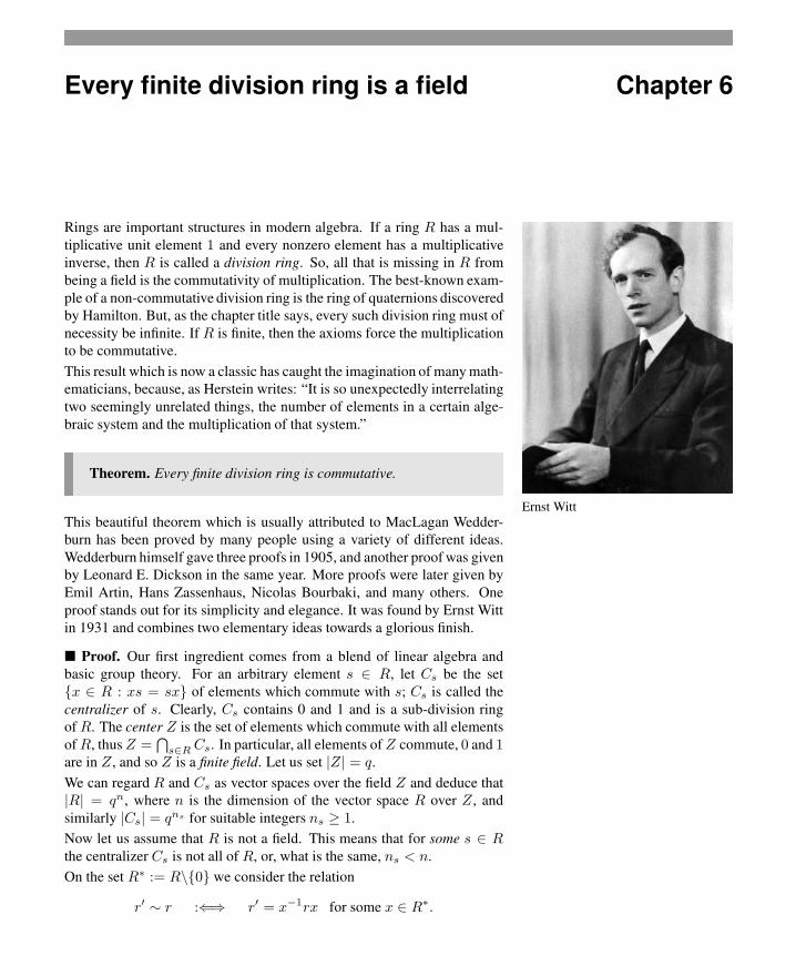
Ernst Witt

Rings are important structures in modern algebra. If a ring R has a mul-tiplicative unit element 1 and every nonzero element has a multiplicativeinverse, then R is called a division ring. So, all that is missing in R frombeing a field is the commutativity of multiplication. The best-known exam-ple of a non-commutative division ring is the ring of quaternions discoveredby Hamilton. But, as the chapter title says, every such division ring must ofnecessity be infinite. If R is finite, then the axioms force the multiplicationto be commutative.

This result which is now a classic has caught the imagination of many math-ematicians, because, as Herstein writes: “It is so unexpectedly interrelatingtwo seemingly unrelated things, the number of elements in a certain alge-braic system and the multiplication of that system.”

Theorem. Every finite division ring is commutative.

This beautiful theorem which is usually attributed to MacLagan Wedder-burn has been proved by many people using a variety of different ideas.Wedderburn himself gave three proofs in 1905, and another proof was givenby Leonard E. Dickson in the same year. More proofs were later given byEmil Artin, Hans Zassenhaus, Nicolas Bourbaki, and many others. Oneproof stands out for its simplicity and elegance. It was found by Ernst Wittin 1931 and combines two elementary ideas towards a glorious finish.

� Proof. Our first ingredient comes from a blend of linear algebra andbasic group theory. For an arbitrary element s ∈ R, let Cs be the set{x ∈ R : xs = sx} of elements which commute with s; Cs is called thecentralizer of s. Clearly, Cs contains 0 and 1 and is a sub-division ringofR. The center Z is the set of elements which commute with all elementsofR, thusZ =

⋂s∈R Cs. In particular, all elements of Z commute, 0 and 1

are in Z , and so Z is a finite field. Let us set |Z| = q.

We can regard R and Cs as vector spaces over the field Z and deduce that|R| = qn, where n is the dimension of the vector space R over Z , andsimilarly |Cs| = qns for suitable integers ns ≥ 1.

Now let us assume that R is not a field. This means that for some s ∈ Rthe centralizer Cs is not all of R, or, what is the same, ns < n.

On the set R∗ := R\{0} we consider the relation

r′ ∼ r :⇐⇒ r′ = x−1rx for some x ∈ R∗.

32 Every finite division ring is a field

It is easy to check that ∼ is an equivalence relation. Let

As := {x−1sx : x ∈ R∗}

be the equivalence class containing s. We note that |As| = 1 preciselywhen s is in the center Z . So by our assumption, there are classes As with|As| ≥ 2. Consider now for s ∈ R∗ the map fs : x 7−→ x−1sx from R∗

onto As. For x, y ∈ R∗ we find

x−1sx = y−1sy ⇐⇒ (yx−1)s = s(yx−1)

⇐⇒ yx−1 ∈ C∗s ⇐⇒ y ∈ C∗

sx,

for C∗s := Cs\{0}, where C∗

sx = {zx : z ∈ C∗s } has size |C∗

s |. Hence anyelement x−1sx is the image of precisely |C∗

s | = qns − 1 elements in R∗

under the map fs, and we deduce |R∗| = |As| |C∗s |. In particular, we note

that|R∗||C∗

s |=

qn − 1

qns − 1= |As| is an integer for all s.

We know that the equivalence classes partition R∗. We now group thecentral elements Z∗ together and denote by A1, . . . , At the equivalenceclasses containing more than one element. By our assumption we knowt ≥ 1. Since |R∗| = |Z∗| +

∑tk=1 |Ak|, we have proved the so-called

class formula

qn − 1 = q − 1 +

t∑

k=1

qn − 1

qnk − 1, (1)

where we have 1 < qn−1qnk−1 ∈ N for all k.

With (1) we have left abstract algebra and are back to the natural numbers.Next we claim that qnk−1 | qn−1 implies nk |n. Indeed, write n = ank+rwith 0 ≤ r < nk, then qnk − 1 | qank+r − 1 implies

qnk − 1 | (qank+r − 1)− (qnk − 1) = qnk(q(a−1)nk+r − 1),

and thus qnk − 1 | q(a−1)nk+r − 1, since qnk and qnk − 1 are relativelyprime. Continuing in this way we find qnk − 1 | qr − 1 with 0 ≤ r < nk,which is only possible for r = 0, that is, nk |n. In summary, we note

nk |n for all k. (2)

Now comes the second ingredient: the complex numbers C. Consider thepolynomial xn − 1. Its roots in C are called the n-th roots of unity. Sinceλn = 1, all these roots λ have |λ| = 1 and lie therefore on the unit circle ofthe complex plane. In fact, they are precisely the numbers λk = e

2kπin =

cos(2kπ/n) + i sin(2kπ/n), 0 ≤ k ≤ n − 1 (see the box on the nextpage). Some of the roots λ satisfy λd = 1 for d < n; for example, theroot λ = −1 satisfies λ2 = 1. For a root λ, let d be the smallest positiveexponent with λd = 1, that is, d is the order of λ in the group of the rootsof unity. Then d |n, by Lagrange’s theorem (“the order of every element of

Every finite division ring is a field 33

a group divides the order of the group” — see the box in Chapter 1). Notethat there are roots of order n, such as λ1 = e

2πin .

Roots of unity

Any complex number z = x+ iy may be written in the “polar” form

z = reiϕ = r(cosϕ+ i sinϕ),

where r = |z| =√x2 + y2 is the distance of z to the origin, and ϕ is

the angle measured from the positive x-axis. The n-th roots of unityare therefore of the form

λk = e2kπi

n = cos(2kπ/n) + i sin(2kπ/n), 0 ≤ k ≤ n− 1,

since for all k

λnk = e2kπi = cos(2kπ) + i sin(2kπ) = 1.

We obtain these roots geometrically by inscribing a regular n-goninto the unit circle. Note that λk = ζk for all k, where ζ = e

2πin . Thus

the n-th roots of unity form a cyclic group {ζ, ζ2, . . . , ζn−1, ζn = 1}of order n.

x = r cosϕ

ϕ

z = reiϕ

y = r sinϕ

r = |z|

︸︷︷︸

−1

λ2 λ1 = ζ

1

The roots of unity for n = 6

Now we group all roots of order d together and set

φd(x) :=∏

λ of order d

(x− λ).

Note that the definition of φd(x) is independent of n. Since every root hassome order d, we conclude that

xn − 1 =∏

d |nφd(x). (3)

Here is the crucial observation: The coefficients of the polynomials φn(x)are integers (that is, φn(x) ∈ Z[x] for all n), where in addition the constantcoefficient is either 1 or −1.

Let us carefully verify this claim. For n = 1 we have 1 as the only root,and so φ1(x) = x − 1. Now we proceed by induction, where we assumeφd(x) ∈ Z[x] for all d < n, and that the constant coefficient of φd(x) is 1or −1. By (3),

xn − 1 = p(x)φn(x) (4)

where p(x) =ℓ∑

j=0

pjxj , φn(x) =

n−ℓ∑k=0

akxk, with p0 = 1 or p0 = −1.

Since −1 = p0a0, we see a0 ∈ {1,−1}. Suppose we already know thata0, a1, . . . , ak−1 ∈ Z. Computing the coefficient of xk on both sides of (4)

34 Every finite division ring is a field

we findk∑

j=0

pjak−j =

k∑

j=1

pjak−j + p0ak ∈ Z.

By assumption, all a0, . . . , ak−1 (and all pj) are in Z. Thus p0ak and henceak must also be integers, since p0 is 1 or −1.

We are ready for the coup de grâce. Let nk |n be one of the numbersappearing in (1). Then

xn − 1 =∏

d |nφd(x) = (xnk − 1)φn(x)

∏

d |n, d∤nk, d6=n

φd(x).

We conclude that in Z we have the divisibility relations

φn(q) | qn − 1 and φn(q)∣∣ q

n − 1

qnk − 1. (5)

Since (5) holds for all k, we deduce from the class formula (1)

φn(q) | q − 1,

but this cannot be. Why? We know φn(x) =∏

(x − λ) where λ runsthrough all roots of xn−1 of order n. Let λ = a+ ib be one of those roots.By n > 1 (because of R 6= Z) we have λ 6= 1, which implies that the realpart a is smaller than 1. Now |λ|2 = a2 + b2 = 1, and hence

|q − λ|2 = |q − a− ib|2 = (q − a)2 + b2

= q2 − 2aq + a2 + b2 = q2 − 2aq + 1

> q2 − 2q + 1 (because of a < 1)

= (q − 1)2,

and so |q − λ| > q − 1 holds for all roots of order n. This implies

1 q

µ

|q − µ| > |q − 1|

|φn(q)| =∏

λ

|q − λ| > q − 1,

which means that φn(q) cannot be a divisor of q− 1, contradiction and endof proof. �

References

[1] L. E. DICKSON: On finite algebras, Nachrichten der Akad. WissenschaftenGöttingen Math.-Phys. Klasse (1905), 1-36; Collected Mathematical PapersVol. III, Chelsea Publ. Comp, The Bronx, NY 1975, 539-574.

[2] J. H. M. WEDDERBURN: A theorem on finite algebras, Trans. Amer. Math.Soc. 6 (1905), 349-352.

[3] E. WITT: Über die Kommutativität endlicher Schiefkörper, Abh. Math. Sem.Univ. Hamburg 8 (1931), 413.

Some irrational numbers Chapter 7

Charles Hermite

“π is irrational”

This was already conjectured by Aristotle, when he claimed that diameterand circumference of a circle are not commensurable. The first proof ofthis fundamental fact was given by Johann Heinrich Lambert in 1766. OurBook Proof is due to Ivan Niven, 1947: an extremely elegant one-pageproof that needs only elementary calculus. Its idea is powerful, and quitea bit more can be derived from it, as was shown by Iwamoto and Koksma,respectively:

• π2 is irrational and

• er is irrational for rational r 6= 0.

Niven’s method does, however, have its roots and predecessors: It can betraced back to the classical paper by Charles Hermite from 1873 whichfirst established that e is transcendental, that is, that e is not a zero of apolynomial with rational coefficients.

e := 1 + 11

+ 12

+ 16

+ 124

+ . . .

= 2.718281828...

ex := 1 + x1

+ x2

2+ x4

6+ x4

24+ . . .

=X

k≥0

xk

k!

Before we treat π we will look at e and its powers, and see that these areirrational. This is much easier, and we thus also follow the historical orderin the development of the results.

To start with, it is rather easy to see (as did Fourier in 1815) that e =∑k≥0

1k! is irrational. Indeed, if we had e = a

b for integers a and b > 0,then we would get

n!be = n!a

for every n ≥ 0. But this cannot be true, because on the right-hand side wehave an integer, while the left-hand side with

e =(1+

1

1!+

1

2!+. . .+

1

n!

)+( 1

(n+ 1)!+

1

(n+ 2)!+

1

(n+ 3)!+ . . .

)

decomposes into an integral part

bn!(1 +

1

1!+

1

2!+ . . .+

1

n!

)

and a second part

b( 1

n+ 1+

1

(n+ 1)(n+ 2)+

1

(n+ 1)(n+ 2)(n+ 3)+ . . .

)

36 Some irrational numbers

which is approximately bn , so that for large n it certainly cannot be integral:

It is larger than bn+1 and smaller than b

n , as one can see from a comparisonwith a geometric series:

1

n+ 1<

1

n+ 1+

1

(n+ 1)(n+ 2)+

1

(n+ 1)(n+ 2)(n+ 3)+ . . .

<1

n+ 1+

1

(n+ 1)2+

1

(n+ 1)3+ . . . =

1

n.

Geometric series

For the infinite geometric series

Q = 1q

+ 1q2 + 1

q3 + . . .

with q > 1 we clearly have

qQ = 1 + 1q

+ 1q2 + . . . = 1 + Q

and thus

Q =1

q − 1.

Now one might be led to think that this simple multiply–by–n! trick is noteven sufficient to show that e2 is irrational. This is a stronger statement:√

2 is an example of a number which is irrational, but whose square is not.

From John Cosgrave we have learned that with two nice ideas/observations(let’s call them “tricks”) one can get two steps further nevertheless: Each ofthe tricks is sufficient to show that e2 is irrational, the combination of bothof them even yields the same for e4. The first trick may be found in a one

Liouville’s paper

page paper by J. Liouville from 1840 — and the second one in a two page“addendum” which Liouville published on the next two journal pages.

Why is e2 irrational? What can we derive from e2 = ab ? According to

Liouville we should write this as

be = ae−1,

substitute the series

e = 1 +1

1+

1

2+

1

6+

1

24+

1

120+ . . .

and

e−1 = 1− 1

1+

1

2− 1

6+

1

24− 1

120± . . . ,

and then multiply by n!, for a sufficiently large even n. Then we see thatn!be is nearly integral:

n!b(1 +

1

1+

1

2+

1

6+ . . .+

1

n!

)

is an integer, and the rest

n!b( 1

(n+ 1)!+

1

(n+ 2)!+ . . .

)

is approximately bn : It is larger than b

n+1 but smaller than bn , as we have

seen above.

At the same time n!ae−1 is nearly integral as well: Again we get a largeintegral part, and then a rest

(−1)n+1n!a( 1

(n+ 1)!− 1

(n+ 2)!+

1

(n+ 3)!∓ . . .

),

Some irrational numbers 37

and this is approximately (−1)n+1 an . More precisely: for even n the rest is

larger than − an , but smaller than

−a( 1

n+ 1− 1

(n+ 1)2− 1

(n+ 1)3− . . .

)= − a

n+ 1

(1− 1

n

)< 0.

But this cannot be true, since for large even n it would imply that n!ae−1 isjust a bit smaller than an integer, while n!be is a bit larger than an integer,so n!ae−1 = n!be cannot hold. �

In order to show that e4 is irrational, we now courageously assume thate4 = a

b were rational, and write this as

be2 = ae−2.

We could now try to multiply this by n! for some large n, and collect thenon-integral summands, but this leads to nothing useful: The sum of theremaining terms on the left-hand side will be approximately b 2n+1

n , on the

right side (−1)n+1a 2n+1

n , and both will be very large if n gets large.

So one has to examine the situation a bit more carefully, and make two littleadjustments to the strategy: First we will not take an arbitrary large n, buta large power of two, n = 2m; and secondly we will not multiply by n!,but by n!

2n−1 . Then we need a little lemma, a special case of Legendre’stheorem (see page 8): For any n ≥ 1 the integer n! contains the primefactor 2 at most n − 1 times — with equality if (and only if) n is a powerof two, n = 2m.

This lemma is not hard to show: ⌊n2 ⌋ of the factors of n! are even, ⌊n

4 ⌋ ofthem are divisible by 4, and so on. So if 2k is the largest power of twowhich satisfies 2k ≤ n, then n! contains the prime factor 2 exactly

⌊n2

⌋+⌊n

4

⌋+ . . .+

⌊ n2k

⌋≤ n

2+n

4+ . . .+

n

2k= n

(1− 1

2k

)≤ n−1

times, with equality in both inequalities exactly if n = 2k.

Let’s get back to be2 = ae−2. We are looking at

bn!

2n−1e2 = a

n!

2n−1e−2 (1)

and substitute the series

e2 = 1 +2

1+

4

2+

8

6+ . . . +

2r

r!+ . . .

and

e−2 = 1− 2

1+

4

2− 8

6± . . . + (−1)r 2r

r!+ . . .

For r ≤ n we get integral summands on both sides, namely

bn!

2n−1

2r

r!resp. (−1)ra

n!

2n−1

2r

r!,


where for r > 0 the denominator r! contains the prime factor 2 at mostr − 1 times, while n! contains it exactly n − 1 times. (So for r > 0 thesummands are even.)

And since n is even (we assume that n = 2m), the series that we get forr ≥ n+ 1 are

2b( 2

n+ 1+

4

(n+ 1)(n+ 2)+

8

(n+ 1)(n+ 2)(n+ 3)+ . . .

)

resp.

2a(− 2

n+ 1+

4

(n+ 1)(n+ 2)− 8

(n+ 1)(n+ 2)(n+ 3)± . . .

).

These series will for large n be roughly 4bn resp. − 4a

n , as one sees again bycomparison with geometric series. For large n = 2m this means that theleft-hand side of (1) is a bit larger than an integer, while the right-hand sideis a bit smaller — contradiction! �

So we know that e4 is irrational; to show that e3, e5 etc. are irrational aswell, we need heavier machinery (that is, a bit of calculus), and a new idea— which essentially goes back to Charles Hermite, and for which the keyis hidden in the following simple lemma.

Lemma. For some fixed n ≥ 1, let

f(x) =xn(1− x)n

n!.

(i) The function f(x) is a polynomial of the form f(x) =1

n!

2n∑

i=n

cixi,

where the coefficients ci are integers.

(ii) For 0 < x < 1 we have 0 < f(x) < 1n! .

(iii) The derivatives f (k)(0) and f (k)(1) are integers for all k ≥ 0.

� Proof. Parts (i) and (ii) are clear.For (iii) note that by (i) the k-th derivative f (k) vanishes at x = 0 unlessn ≤ k ≤ 2n, and in this range f (k)(0) = k!

n!ck is an integer. From f(x) =

f(1−x) we get f (k)(x) = (−1)kf (k)(1−x) for all x, and hence f (k)(1) =(−1)kf (k)(0), which is an integer. �

Theorem 1. er is irrational for every r ∈ Q\{0}.

� Proof. It suffices to show that es cannot be rational for a positive integers (if e

st were rational, then

(e

st

)t= es would be rational, too). Assume

that es = ab for integers a, b > 0, and let n be so large that n! > as2n+1.

PutThe estimate n! > e(n

e)n yields an

explicit n that is “large enough.”

F (x) := s2nf(x)− s2n−1f ′(x) + s2n−2f ′′(x) ∓ . . . + f (2n)(x),

where f(x) is the function of the lemma.


F (x) may also be written as an infinite sum

F (x) = s2nf(x)− s2n−1f ′(x) + s2n−2f ′′(x)∓ . . . ,

since the higher derivatives f (k)(x), for k > 2n, vanish. From this we seethat the polynomial F (x) satisfies the identity

F ′(x) = −s F (x) + s2n+1f(x).

Thus differentiation yields

d

dx[esxF (x)] = sesxF (x) + esxF ′(x) = s2n+1esxf(x)

and hence

N := b

∫ 1

0

s2n+1esxf(x)dx = b [esxF (x)]10 = aF (1)− bF (0).

This is an integer, since part (iii) of the lemma implies that F (0) and F (1)are integers. However, part (ii) of the lemma yields estimates for the sizeof N from below and from above,

0 < N = b

∫ 1

0

s2n+1esxf(x)dx < bs2n+1es 1

n!=

as2n+1

n!< 1,

which shows that N cannot be an integer: contradiction. �

Now that this trick was so successful, we use it once more.

Theorem 2. π2 is irrational.

� Proof. Assume that π2 = ab for integers a, b > 0. We now use the

polynomial

F (x) := bn(π2nf(x)− π2n−2f (2)(x) + π2n−4f (4)(x)∓ . . .

),

which satisfies F ′′(x) = −π2F (x) + bnπ2n+2f(x).

π is not rational, but it does have “goodapproximations” by rationals — someof these were known since antiquity:

227

= 3.142857142857...355113

= 3.141592920353...10434833215

= 3.141592653921...

π = 3.141592653589...

From part (iii) of the lemma we get that F (0) and F (1) are integers.Elementary differentiation rules yield

d

dx

[F ′(x) sin πx− πF (x) cos πx

]=

(F ′′(x) + π2F (x)

)sinπx

= bnπ2n+2f(x) sinπx

= π2anf(x) sinπx,

and thus we obtain

N := π

∫ 1

0

anf(x) sinπxdx =[ 1

πF ′(x) sin πx− F (x) cos πx

]10

= F (0) + F (1),

which is an integer. Furthermore N is positive since it is defined as the


integral of a function that is positive (except on the boundary). However,if we choose n so large that πan

n! < 1, then from part (ii) of the lemma weobtain

0 < N = π

∫ 1

0

anf(x) sinπxdx <πan

n!< 1,

a contradiction. �

Here comes our final irrationality result.

Theorem 3. For every odd integer n ≥ 3, the number

A(n) :=1

πarccos

(1√n

)

is irrational.

We will need this result for Hilbert’s third problem (see Chapter 9) in thecases n = 3 and n = 9. For n = 2 and n = 4 we have A(2) = 1

4 andA(4) = 1

3 , so the restriction to odd integers is essential. These valuesare easily derived by appealing to the diagram in the margin, in which thestatement “ 1

π arccos(

1√n

)is irrational” is equivalent to saying that the

polygonal arc constructed from 1√n

, all of whose chords have the samelength, never closes into itself.

1√n

0 1

We leave it as an exercise for the reader to show that A(n) is rational onlyfor n ∈ {1, 2, 4}. For that, distinguish the cases when n = 2r, and when nis not a power of 2.

� Proof. We use the addition theorem

cosα+ cosβ = 2 cos α+β2 cos α−β

2

from elementary trigonometry, which for α = (k + 1)ϕ and β = (k − 1)ϕyields

cos (k + 1)ϕ = 2 cosϕ cos kϕ − cos (k − 1)ϕ. (2)

For the angle ϕn = arccos(

1√n

), which is defined by cosϕn = 1√

nand

0 ≤ ϕn ≤ π, this yields representations of the form

cos kϕn =Ak√n

k,

where Ak is an integer that is not divisible by n, for all k ≥ 0. In fact,we have such a representation for k = 0, 1 with A0 = A1 = 1, and byinduction on k using (2) we get for k ≥ 1

cos (k + 1)ϕn = 21√n

Ak√n

k− Ak−1√

nk−1

=2Ak − nAk−1√

nk+1

.

Thus we obtain Ak+1 = 2Ak − nAk−1. If n ≥ 3 is odd, and Ak is notdivisible by n, then we find that Ak+1 cannot be divisible by n, either.


Now assume that

A(n) =1

πϕn =

k

ℓ

is rational (with integers k, ℓ > 0). Then ℓϕn = kπ yields

±1 = cos kπ =Aℓ√n

ℓ.

Thus√n

ℓ= ±Aℓ is an integer, with ℓ ≥ 2, and hence n | √nℓ

. With√n

ℓ |Aℓ we find that n dividesAℓ, a contradiction. �

References

[1] C. HERMITE: Sur la fonction exponentielle, Comptes rendus de l’Académiedes Sciences (Paris) 77 (1873), 18-24; Œuvres de Charles Hermite, Vol. III,Gauthier-Villars, Paris 1912, pp. 150-181.

[2] Y. IWAMOTO: A proof that π2 is irrational, J. Osaka Institute of Science andTechnology 1 (1949), 147-148.

[3] J. F. KOKSMA: On Niven’s proof that π is irrational, Nieuw Archief voorWiskunde (2) 23 (1949), 39.

[4] J. LIOUVILLE: Sur l’irrationalité du nombre e = 2,718..., Journal de Mathé-matiques Pures et Appl. (1) 5 (1840), 192; Addition, 193-194.

[5] I. NIVEN: A simple proof that π is irrational, Bulletin Amer. Math. Soc. 53

(1947), 509.

Three times π2/6 Chapter 8

We know that the infinite series∑

n≥11n does not converge. Indeed, in

Chapter 1 we have seen that even the series∑

p∈P1p diverges.

However, the sum of the reciprocals of the squares converges (althoughvery slowly, as we will also see), and it produces an interesting value.

Euler’s series. ∑

n≥1

1

n2=

π2

6.

This is a classical, famous and important result by Leonhard Euler from1734. One of its key interpretations is that it yields the first non-trivial

1 = 1.0000001+ 1

4= 1.250000

1+ 14+ 1

9= 1.361111

1+ 14+ 1

9+ 1

16= 1.423611

1+ 14+ 1

9+ 1

16+ 1

25= 1.463611

1+ 14+ 1

9+ 1

16+ 1

25+ 1

36= 1.491388

π2/6 = 1.644934.

value ζ(2) of Riemann’s zeta function (see the appendix on page 49). Thisvalue is irrational, as we have seen in Chapter 7.

But not only the result has a prominent place in mathematics history, thereare also a number of extremely elegant and clever proofs that have theirhistory: For some of these the joy of discovery and rediscovery has beenshared by many. In this chapter, we present three such proofs.

� Proof. The first proof appears as an exercise in William J. LeVeque’snumber theory textbook from 1956. But he says: “I haven’t the slightestidea where that problem came from, but I’m pretty certain that it wasn’toriginal with me.”

The proof consists in two different evaluations of the double integral

I :=

1∫

0

1∫

0

1

1− xy dx dy.

For the first one, we expand 11−xy as a geometric series, decompose the

summands as products, and integrate effortlessly:

I =

1∫

0

1∫

0

∑

n≥0

(xy)n dx dy =∑

n≥0

1∫

0

1∫

0

xnyn dx dy

=∑

n≥0

( 1∫

0

xndx

)( 1∫

0

yndy

)=∑

n≥0

1

n+ 1

1

n+ 1

=∑

n≥0

1

(n+ 1)2=∑

n≥1

1

n2= ζ(2).

44 Three times π2/6

This evaluation also shows that the double integral (over a positive functionwith a pole at x = y = 1) is finite. Note that the computation is also easyand straightforward if we read it backwards — thus the evaluation of ζ(2)leads one to the double integral I .

1

x

uy

1

v

The second way to evaluate I comes from a change of coordinates: in thenew coordinates given by u := y+x

2 and v := y−x2 the domain of integra-

tion is a square of side length 12

√2, which we get from the old domain by

first rotating it by 45◦ and then shrinking it by a factor of√

2. Substitutionof x = u− v and y = u+ v yields

1

1− xy =1

1− u2 + v2.

To transform the integral, we have to replace dx dy by 2 du dv, to com-pensate for the fact that our coordinate transformation reduces areas by aconstant factor of 2 (which is the Jacobi determinant of the transformation;see the box on the next page). The new domain of integration, and thefunction to be integrated, are symmetric with respect to the u-axis, so wev

I1 u

1

12

12

I2

just need to compute two times (another factor of 2 arises here!) the inte-gral over the upper half domain, which we split into two parts in the mostnatural way:

I = 4

1/2∫

0

( u∫

0

dv

1− u2 + v2

)du + 4

1∫

1/2

( 1−u∫

0

dv

1− u2 + v2

)du.

Using∫

dx

a2 + x2=

1

aarctan

x

a+ C , this becomes

I = 4

1/2∫

0

1√1− u2

arctan

(u√

1− u2

)du

+ 4

1∫

1/2

1√1− u2

arctan

(1− u√1− u2

)du.

These integrals can be simplified and finally evaluated by substituting u =sin θ resp. u = cos θ. But we proceed more directly, by computing that thederivative of g(u) := arctan

(u√

1−u2

)is g′(u) = 1√

1−u2, while the deriva-

tive of h(u) := arctan(

1−u√1−u2

)= arctan

(√1−u1+u

)is h′(u) = − 1

21√

1−u2.

So we may use∫ b

af ′(x)f(x)dx =

[12f(x)2

]ba

= 12f(b)2− 1

2f(a)2 and get

I = 4

∫ 1/2

0

g′(u)g(u) du + 4

∫ 1

1/2

−2h′(u)h(u) du

= 2[g(u)2

]1/2

0− 4

[h(u)2

]11/2

= 2g(12 )2 − 2g(0)2 − 4h(1)2 + 4h(1

2 )2

= 2(

π6

)2 − 0− 0 + 4(

π6

)2= π2

6 . �

Three times π2/6 45

This proof extracted the value of Euler’s series from an integral via a rathersimple coordinate transformation. An ingenious proof of this type — withan entirely non-trivial coordinate transformation — was later discovered byBeukers, Calabi and Kolk. The point of departure for that proof is to splitthe sum

∑n≥1

1n2 into the even terms and the odd terms. Clearly the even

terms 122 + 1

42 + 162 + . . . =

∑k≥1

1(2k)2 sum to 1

4ζ(2), so the odd terms112 + 1

32 + 152 + . . . =

∑k≥0

1(2k+1)2 make up three quarters of the total

sum ζ(2). Thus Euler’s series is equivalent to

The Substitution Formula

To compute a double integral

I =

Z

S

f(x, y) dx dy.

we may perform a substitution ofvariables

x = x(u, v) y = y(u, v),

if the correspondence of (u, v) ∈ Tto (x, y) ∈ S is bijective and contin-uously differentiable. Then I equalsZ

T

f(x(u, v), y(u, v))˛

˛

˛

d(x, y)

d(u, v)

˛

˛

˛du dv,

where d(x,y)d(u,v)

is the Jacobi determi-nant:

d(x, y)

d(u, v)= det

dxdu

dxdv

dydu

dydv

!

.

∑

k≥0

1

(2k + 1)2=

π2

8.

� Proof. As above, we may express this as a double integral, namely

J =

1∫

0

1∫

0

1

1− x2y2dx dy =

∑

k≥0

1

(2k + 1)2.

So we have to compute this integral J . And for this Beukers, Calabi andKolk proposed the new coordinates

u := arccos

√1− x2

1− x2y2v := arccos

√1− y2

1− x2y2.

To compute the double integral, we may ignore the boundary of the domain,and consider x, y in the range 0 < x < 1 and 0 < y < 1. Then u, v will liein the triangle u > 0, v > 0, u + v < π/2. The coordinate transformationcan be inverted explicitly, which leads one to the substitution

x =sinu

cos vand y =

sin v

cosu.

It is easy to check that these formulas define a bijective coordinate transfor-mation between the interior of the unit square S = {(x, y) : 0 ≤ x, y ≤ 1}and the interior of the triangle T = {(u, v) : u, v ≥ 0, u+ v ≤ π/2}.Now we have to compute the Jacobi determinant of the coordinate transfor-mation, and magically it turns out to be

det

(cos ucos v

sin u sin vcos2 v

sin u sin vcos2 u

cos vcos u

)= 1− sin2 u sin2 v

cos2 u cos2 v= 1− x2y2.

But this means that the integral that we want to compute is transformed into

1

S

T

y

1

x

π2

v

π2

uJ =

π/2∫

0

π/2−u∫

0

1 du dv,

which is just the area 12 (π

2 )2 = π2

8 of the triangle T . �


Beautiful — even more so, as the same method of proof extends to thecomputation of ζ(2k) in terms of a 2k-dimensional integral, for all k ≥ 1.We refer to the original paper of Beuker, Calabi and Kolk [2], and toChapter 23, where we’ll achieve this on a different path, using the Herglotztrick and Euler’s original approach.

After these two proofs via coordinate transformation we can’t resist thetemptation to present another, entirely different and completely elementaryproof for

∑n≥1

1n2 = π2

6 . It appears in a sequence of exercises in theproblem book by the twin brothers Akiva and Isaak Yaglom, whose Russianoriginal edition appeared in 1954. Versions of this beautiful proof wererediscovered and presented by F. Holme (1970), I. Papadimitriou (1973),and by Ransford (1982) who attributed it to John Scholes.

� Proof. The first step is to establish a remarkable relation between valuesof the (squared) cotangent function. Namely, for all m ≥ 1 one has

For m = 1, 2, 3 this yieldscot2 π

3= 1

3

cot2 π5

+ cot2 2π5

= 2

cot2 π7

+ cot2 2π7

+ cot2 3π7

= 5

cot2(

π2m+1

)+ cot2

(2π

2m+1

)+ . . .+ cot2

(mπ

2m+1

)= 2m(2m−1)

6 . (1)

To establish this, we start with the relation eix = cosx + i sinx. Takingthe n-th power einx = (eix)n, we get

cosnx+ i sinnx = (cos x+ i sinx)n.

The imaginary part of this is

sinnx =

(n

1

)sinx cosn−1 x−

(n

3

)sin3 x cosn−3 x± . . . (2)

Now we let n = 2m + 1, while for x we will consider the m differentvalues x = rπ

2m+1 , for r = 1, 2, . . . ,m. For each of these values we havenx = rπ, and thus sinnx = 0, while 0 < x < π

2 implies that for sinx weget m distinct positive values.

In particular, we can divide (2) by sinn x, which yields

0 =

(n

1

)cotn−1 x−

(n

3

)cotn−3 x± . . . ,

that is,

0 =

(2m+ 1

1

)cot2m x−

(2m+ 1

3

)cot2m−2 x± . . .

for each of the m distinct values of x. Thus for the polynomial of degreem

p(t) :=

(2m+ 1

1

)tm −

(2m+ 1

3

)tm−1 ± . . .+ (−1)m

(2m+ 1

2m+ 1

)

we know m distinct roots

ar = cot2(

rπ2m+1

)for r = 1, 2, . . . ,m.

Hence the polynomial coincides with

p(t) =

(2m+ 1

1

)(t− cot2

(π

2m+1

))· · ·(t− cot2

(mπ

2m+1

)).


Comparison of the coefficients of tm−1 in p(t) now yields that the sum ofthe roots is

a1 + . . .+ ar =

(2m+1

3

)(2m+1

1

) = 2m(2m−1)6 ,

which proves (1).

Comparison of coefficients:If p(t) = c(t − a1) · · · (t − am),then the coefficient of tm−1 is−c(a1 + . . . + am).

We also need a second identity, of the same type,

csc2(

π2m+1

)+ csc2

(2π

2m+1

)+ . . .+ csc2

(mπ

2m+1

)= 2m(2m+2)

6 , (3)

for the cosecant function cscx = 1sin x . But

csc2 x =1

sin2 x=

cos2 x+ sin2 x

sin2 x= cot2 x+ 1,

so we can derive (3) from (1) by adding m to both sides of the equation.

Now the stage is set, and everything falls into place. We use that in therange 0 < y < π

2 we have

0 < a < b < c

implies

0 < 1c

< 1b

< 1a

0 < sin y < y < tan y,

and thus

0 < cot y < 1y < csc y,

which implies

cot2 y < 1y2 < csc2 y.

Now we take this double inequality, apply it to each of them distinct valuesof x, and add the results. Using (1) for the left-hand side, and (3) for theright-hand side, we obtain

2m(2m−1)6 <

(2m+1

π

)2+(

2m+12π

)2+ . . .+

(2m+1mπ

)2< 2m(2m+2)

6 ,

that is,

π2

62m

2m+12m−12m+1 < 1

12 + 122 + . . .+ 1

m2 < π2

62m

2m+12m+22m+1 .

Both the left-hand and the right-hand side converge to π2

6 for m −→ ∞:end of proof. �

So how fast does∑ 1

n2 converge to π2/6? For this we have to estimate thedifference

π2

6−

m∑

n=1

1

n2=

∞∑

n=m+1

1

n2.


This is very easy with the technique of “comparing with an integral” thatwe have reviewed already in the appendix to Chapter 2 (page 10). It yields

. . .m+ 1

1(m+1)2

f(t) = 1t2

t

∞∑

n=m+1

1

n2<

∫ ∞

m

1

t2dt =

1

m

for an upper bound and∞∑

n=m+1

1

n2>

∫ ∞

m+1

1

t2dt =

1

m+ 1

for a lower bound on the “remaining summands” — or even∞∑

n=m+1

1

n2>

∫ ∞

m+ 12

1

t2dt =

1

m+ 12

if you are willing to do a slightly more careful estimate, using that thefunction f(t) = 1

t2 is convex.

This means that our series does not converge too well; if we sum the firstone thousand summands, then we expect an error in the third digit afterthe decimal point, while for the sum of the first one million summands,m = 1000000, we expect to get an error in the sixth decimal digit, andwe do. However, then comes a big surprise: to an accuracy of 45 digits,

π2/6 = 1.644934066848226436472415166646025189218949901,

106∑

n=1

1

n2= 1.644933066848726436305748499979391855885616544.

So the sixth digit after the decimal point is wrong (too small by 1), butthe next six digits are right! And then one digit is wrong (too large by 5),then again five are correct. This surprising discovery is quite recent, due toRoy D. North from Colorado Springs, 1988. (In 1982, Martin R. Powell,a school teacher from Amersham, Bucks, England, failed to notice the fulleffect due to the insufficient computing power available at the time.) It istoo strange to be purely coincidental . . . A look at the error term, whichagain to 45 digits reads

∞∑

n=106+1

1

n2= 0.000000999999500000166666666666633333333333357,

reveals that clearly there is a pattern. You might try to rewrite this lastnumber as

+ 10−6 − 1210−12 + 1

610−18 − 13010−30 + 1

4210−42 + . . .

where the coefficients (1,− 12 ,

16 , 0,− 1

30 , 0,142 ) of 10−6i form the be-

ginning of the sequence of Bernoulli numbers that we’ll meet again inChapter 23. We refer our readers to the article by Borwein, Borwein &Dilcher [3] for more such surprising “coincidences” — and for proofs.


Appendix: The Riemann zeta function

The Riemann zeta function ζ(s) is defined for real s > 1 by

ζ(s) :=∑

n≥1

1

ns.

Our estimates for Hn (see page 10) imply that the series for ζ(1) diverges,but for any real s > 1 it does converge. The zeta function has a canonicalcontinuation to the entire complex plane (with one simple pole at s = 1),which can be constructed using power series expansions. The resultingcomplex function is of utmost importance for the theory of prime numbers.Let us mention four diverse connections:

(1) The remarkable identity

ζ(s) =∏

p

1

1− p−s

is due to Euler. It encodes the basic fact that every natural number has aunique (!) decomposition into prime factors; using this, Euler’s identity isa simple consequence of the geometric series expansion

1

1− p−s= 1 +

1

ps+

1

p2s+

1

p3s+ . . .

(2) The following marvelous argument of Don Zagier computes ζ(4)from ζ(2). Consider the function

f(m,n) =2

m3n+

1

m2n2+

2

mn3

for integers m,n ≥ 1. It is easily verified that for all m and n,

f(m,n)− f(m+ n, n)− f(m,m+ n) =2

m2n2.

Let us sum this equation over all m,n ≥ 1. If i 6= j, then (i, j) is either ofthe form (m+ n, n) or of the form (m,m+ n), for m,n ≥ 1. Thus, in thesum on the left-hand side all terms f(i, j) with i 6= j cancel, and so

∑

n≥1

f(n, n) =∑

n≥1

5

n4= 5ζ(4)

remains. For the right-hand side one obtains

∑

m,n≥1

2

m2n2= 2

∑

m≥1

1

m2·∑

n≥1

1

n2= 2ζ(2)2,

and out comes the equality

5ζ(4) = 2ζ(2)2.

With ζ(2) = π2

6 we thus get ζ(4) = π4

90 .

Another derivation via Bernoulli numbers appears in Chapter 23.


(3) It has been known for a long time that ζ(s) is a rational multipleof πs, and hence irrational, if s is an even integer s ≥ 2; see Chapter 23.In contrast, the irrationality of ζ(3) was proved by Roger Apéry only in1979. Despite considerable effort the picture is rather incomplete aboutζ(s) for the other odd integers, s = 2t+ 1 ≥ 5. Very recently, Keith Balland Tanguy Rivoal proved that infinitely many of the values ζ(2t + 1) areirrational. And indeed, although it is not known for any single odd values ≥ 5 that ζ(s) is irrational, Wadim Zudilin has proved that at least oneof the four values ζ(5), ζ(7), ζ(9), and ζ(11) is irrational. We refer to thebeautiful survey by Fischler.

(4) The location of the complex zeros of the zeta function is the subjectof the “Riemann hypothesis”: one of the most famous and important unre-solved conjectures in all of mathematics. It claims that all the non-trivialzeros s ∈ C of the zeta function satisfy Re(s) = 1

2 . (The zeta functionvanishes at all the negative even integers, which are referred to as the“trivial zeros.”)

Very recently, Jeff Lagarias showed that, surprisingly, the Riemann hypo-thesis is equivalent to the following elementary statement: For all n ≥ 1,

∑

d |nd ≤ Hn + exp(Hn) log(Hn),

with equality only for n = 1, whereHn is again the n-th harmonic number.

References

[1] K. BALL & T. RIVOAL: Irrationalité d’une infinité de valeurs de la fonctionzêta aux entiers impairs, Inventiones math. 146 (2001), 193-207.

[2] F. BEUKERS, J. A. C. KOLK & E. CALABI: Sums of generalized harmonicseries and volumes, Nieuw Archief voor Wiskunde (4) 11 (1993), 217-224.

[3] J. M. BORWEIN, P. B. BORWEIN & K. DILCHER: Pi, Euler numbers, andasymptotic expansions, Amer. Math. Monthly 96 (1989), 681-687.

[4] S. FISCHLER: Irrationalité de valeurs de zêta (d’après Apéry, Rivoal, . . . ),Bourbaki Seminar, No. 910, November 2002; Astérisque 294 (2004), 27-62.

[5] J. C. LAGARIAS: An elementary problem equivalent to the Riemann hypo-thesis, Amer. Math. Monthly 109 (2002), 534-543.

[6] W. J. LEVEQUE: Topics in Number Theory, Vol. I, Addison-Wesley, ReadingMA 1956.

[7] A. M. YAGLOM & I. M. YAGLOM: Challenging mathematical problems withelementary solutions, Vol. II, Holden-Day, Inc., San Francisco, CA 1967.

[8] D. ZAGIER: Values of zeta functions and their applications, Proc. First Euro-pean Congress of Mathematics, Vol. II (Paris 1992), Progress in Math. 120,Birkhäuser, Basel 1994, pp. 497-512.

[9] W. ZUDILIN: Arithmetic of linear forms involving odd zeta values, J. ThéorieNombres Bordeaux 16 (2004), 251-291.

Proofs from THE BOOK 269

About the Illustrations

We are happy to have the possibility and privilege to illustrate this volumewith wonderful original drawings by Karl Heinrich Hofmann (Darmstadt).Thank you!The regular polyhedra on page 76 and the fold-out map of a flexible sphereon page 84 are by WAF Ruppert (Vienna). Jürgen Richter-Gebert (Munich)provided the two illustrations on page 78, and Ronald Wotzlaw wrote thenice postscript graphics for page 134.Page 231 features the Weisman Art Museum in Minneapolis designed byFrank Gehry. The photo of its west façade is by Chris Faust. The floorplanis of the Dolly Fiterman Riverview Gallery behind the west façade.The portraits of Bertrand, Cantor, Erdos, Euler, Fermat, Herglotz, Hermite,Hilbert, Pólya, Littlewood, and Sylvester are all from the photo archivesof the Mathematisches Forschungsinstitut Oberwolfach, with permission.(Many thanks to Annette Disch!)The Gauss portrait on page 23 is a lithograph by Siegfried Detlev Bendixenpublished in Astronomische Nachrichten 1828, as provided by Wikipedia.The picture of Hermite is from the first volume of his collected works.The Eisenstein portrait is reproduced with friendly permission by Prof.Karin Reich from a collection of portrait cards owned by the Mathema-tische Gesellschaft Hamburg.The portrait stamps of Buffon, Chebyshev, Euler, and Ramanujan are fromJeff Miller’s mathematical stamps website http://jeff560.tripod.com withhis generous permission.The photo of Claude Shannon was provided by the MIT Museum and ishere reproduced with their permission.The portrait of Cayley is taken from the “Photoalbum für Weierstraß”(edited by Reinhard Bölling, Vieweg 1994), with permission from the Kunst-bibliothek, Staatliche Museen zu Berlin, Preussischer Kulturbesitz.The Cauchy portrait is reproduced with permission from the Collections del’École Polytechnique, Paris. The picture of Fermat is reproduced from Ste-fan Hildebrandt and Anthony Tromba: The Parsimonious Universe. Shapeand Form in the Natural World, Springer-Verlag, New York 1996.The portrait of Ernst Witt is from volume 426 (1992) of the Journal für dieReine und Angewandte Mathematik, with permission by Walter de GruyterPublishers. It was taken around 1941.The photo of Karol Borsuk was taken in 1967 by Isaac Namioka, and isreproduced with his kind permission.We thank Dr. Peter Sperner (Braunschweig) for the portrait of his father,and Vera Sós for the photo of Paul Turán.Thanks to Noga Alon for the portrait of A. Nilli!

Index

acyclic directed graph, 196addition theorems, 150adjacency matrix, 248adjacent vertices, 66antichain, 179arithmetic mean, 119art gallery theorem, 232average degree, 76average number of divisors, 164

Bernoulli numbers, 48, 152Bertrand’s postulate, 7bijection, 103, 207Binet–Cauchy formula, 197, 203binomial coefficient, 13bipartite graph, 67, 223birthday paradox, 185Bolyai–Gerwien Theorem, 53Borsuk’s conjecture, 95Borsuk–Ulam theorem, 252Bricard’s condition, 57Brouwer’s fixed point theorem, 169Buffon’s needle problem, 155

Calkin–Wilf tree, 105Cantor–Bernstein theorem, 110capacity, 242cardinal number, 103cardinality, 103, 115Cauchy’s arm lemma, 82Cauchy’s minimum principle, 127Cauchy’s rigidity theorem, 81Cauchy–Schwarz inequality, 119Cayley’s formula, 201center, 31centralizer, 31centrally symmetric, 61chain, 179channel, 241Chebyshev polynomials, 144

Chebyshev’s theorem, 140chromatic number, 221, 251class formula, 32clique, 67, 235, 242clique number, 2372-colorable set system, 261combinatorially equivalent, 61comparison of coefficients, 47complete bipartite graph, 66complete graph, 66complex polynomial, 139components of a graph, 67cone lemma, 56confusion graph, 241congruent, 61connected, 67connected components, 67continuum, 109continuum hypothesis, 112convex polytope, 59convex vertex, 232cosine polynomial, 143countable, 103coupon collector’s problem, 186critical family, 182crossing lemma, 267crossing number, 266cube, 60cycle, 67C4-condition, 257C4-free graph, 166

degree, 76dense, 114determinants, 195dihedral angle, 57dimension, 109dimension of a graph, 162Dinitz problem, 221directed graph, 223

272 Index

division ring, 31double counting, 164dual graph, 75, 227

edge of a graph, 66edge of a polyhedron, 60elementary polygon, 79equal size, 103equicomplementability, 54equicomplementable polyhedra, 53equidecomposability, 54equidecomposable polyhedra, 53Erdos–Ko–Rado theorem, 180Euler’s criterion, 24Euler’s function, 28Euler’s polyhedron formula, 75Euler’s series, 43even function, 152expectation, 94

face, 60, 75facet, 60Fermat number, 3finite field, 31finite fields, 28finite set system, 179forest, 67formal power series, 207four-color theorem, 227friendship theorem, 257fundamental theorem of algebra, 127

Gale’s theorem, 253Gauss lemma, 25Gauss sum, 27general position, 253geometric mean, 119Gessel–Viennot lemma, 195girth, 263golden section, 245graph, 66graph coloring, 227graph of a polytope, 60

harmonic mean, 119harmonic number, 10Herglotz trick, 149Hilbert’s third problem, 53

hyper-binary representation, 106

incidence matrix, 64, 164incident, 66indegree, 223independence number, 241, 251, 264independent set, 67, 221induced subgraph, 67, 222inequalities, 119infinite products, 207initial ordinal number, 116intersecting family, 180, 251involution, 20irrational numbers, 35isomorphic graphs, 67

Jacobi determinants, 45

kernel, 223Kneser graph, 251Kneser’s conjecture, 252

labeled tree, 201Lagrange’s theorem, 4Latin rectangle, 214Latin square, 213, 221lattice, 79lattice basis, 80lattice paths, 195lattice points, 26law of quadratic reciprocity, 24Legendre symbol, 23Legendre’s theorem, 8lexicographically smallest solution, 56line graph, 226linear extension, 176linearity of expectation, 94, 156list chromatic number, 222list coloring, 222, 228Littlewood–Offord problem, 145loop, 66Lovász’ theorem, 247Lovász umbrella, 244Lyusternik–Shnirel’man theorem, 252

Markov’s inequality, 94marriage theorem, 182matching, 224matrix of rank 1, 96

Index 273

matrix-tree theorem, 203Mersenne number, 4Minkowski symmetrization, 91mirror image, 61monotone subsequences, 162Monsky’s Theorem, 133multiple edges, 66museum guards, 231Mycielski graph, 264

near-triangulated plane graph, 228nearly-orthogonal vectors, 96needles, 155neighbors, 66Newman’s function, 107non-Archimedean real valuation, 132non-Archimedean valuation, 136

obtuse angle, 89odd function, 150order of a group element, 4ordered abelian group, 136ordered set, 115ordinal number, 115orthonormal representation, 244outdegree, 223

p-adic value, 132partial Latin square, 213partition, 207partition identities, 207path, 67path matrix, 195pearl lemma, 55pentagonal numbers, 209periodic function, 150Petersen graph, 251Pick’s theorem, 79pigeon-hole principle, 161planar graph, 75plane graph, 75, 228point configuration, 69polygon, 59polyhedron, 53, 59polynomial with real roots, 121, 142polytope, 89prime field, 18prime number, 3, 7

prime number theorem, 10probabilistic method, 261probability distribution, 236probability space, 94product of graphs, 241projective plane, 167

quadratic nonresidue, 23quadratic reciprocity, 24quadratic residue, 23

rainbow triangle, 133Ramsey number, 262random variable, 94rate of transmission, 241red-blue segment, 135refining sequence, 205Riemann zeta function, 49riffle shuffles, 191Rogers–Ramanujan identities, 211rooted forest, 205roots of unity, 33

scalar product, 96Schönhardt’s polyhedron, 232segment, 54Shannon capacity, 242shuffling cards, 185simple graph, 66simplex, 60size of a set, 103slope problem, 69speed of convergence, 47Sperner’s lemma, 169Sperner’s theorem, 179squares, 18stable matching, 224star, 65Stern’s diatomic series, 104Stirling’s formula, 11stopping rules, 188subgraph, 67sums of two squares, 17Sylvester’s theorem, 13Sylvester–Gallai theorem, 63, 78system of distinct representatives, 181

274 Index

tangential rectangle, 121tangential triangle, 121top-in-at-random shuffles, 187touching simplices, 85tree, 67triangle-free graph, 264Turán graph, 235Turán’s graph theorem, 235two square theorem, 17

umbrella, 244unimodal, 12unit d-cube, 60

valuation ring, 136valuations, 131, 136vertex, 60, 66vertex degree, 76, 165, 222vertex-disjoint path system, 195volume, 84

weighted directed graph, 195well-ordered, 115well-ordering theorem, 115windmill graph, 257

zero-error capacity, 242Zorn’s lemma, 137

is prof aba power of - university of wisconsin–eau claire of proofs from the...hello prospective...

Documents