Is it the "How" or the "When" that Mattersin Fiscal Adjustments?∗

Alberto Alesina, Gualtiero Azzalini, Carlo Favero,Francesco Giavazzi and Armando Miano†

First draft: April 2016Revised: October 2016

Abstract

Using data from 16 OECD countres from 1981 to 2014, we find thatthe composition of fiscal adjustments is much more important thanthe state of the cycle in determining their effects on output. Fiscaladjustments based upon spending cuts are much less costly than thosebased upon tax increases, regardless of whether the adjustment startsin a recession or not.

∗Prepared for the 2016 IMF-ARC conference. We thank two anonymous refereesfor very useful comments on an early draft.†Harvard and Igier Bocconi; NYU Stern; Igier Bocconi; Igier Bocconi; Harvard.

1

1 Introduction

The empirical literature on the macroeconomic effects of fiscal policy oftenfinds that fiscal multipliers depend on the state of the economy: whethera shift in fiscal policy happens during an economic expansion or during acontraction makes a difference. Is this the relevant non-linearity when dealingwith fiscal adjustments? This paper studies whether what matters most isthe "when" (whether an adjustment is carried out during an expansion, or arecession) or the "how" (i.e. the composition of the adjustment, whether itis mostly based on tax increases, or on spending cuts). In order to properlyanswer this question one needs to study the two aspects —the "when" and the"how" —jointly, otherwise one risks attributing to one source of non-linearityeffects that are really produced by the other. So far this has not been donein the literature which has typically studied the two aspects separately. Thispaper fills the gap.We estimate a model which allows for both sources of non-linearity:

"when" and "how". We find that the composition of fiscal adjustments ismore important than the state of the cycle in determining their effect onoutput. Fiscal adjustments based upon spending cuts are much less costlyin terms of short run output losses – such losses are in fact on average closeto zero – than those based upon tax increases which are associated withlarge and prolonged recessions regardless of whether the adjustment starts ina recession or not. The dynamic response of the economy to a consolidationprogram does depend on whether this is adopted in a period of economicexpansion or contraction, but the quantitative significance of this source ofnon-linearity is small relative to the one which depends on the type of consol-idation. Our results appear not to be systematically explained by differentreactions of monetary policy and, therefore, they should survive at the zerolower bound (ZLB) when monetary policy is constrained, or within mone-tary unions where monetary policy cannot respond to the fiscal policy of aspecific member country. We find, however, that in one case the response ofmonetary policy appears to make a difference. When the domestic centralbank can set interest rates —that is outside of a currency union —it appearsto be able to dampen the recessionary effects of tax-based consolidationsimplemented during a recession. This finding could help understand the re-cessionary effects of European "Austerity", which was mostly tax based andimplemented within a currency union.Auerbach and Gorodnichenko 2012, 2013 find that GDP multipliers of

government purchases are larger in recessions. Barnichon and Matthes 2015find that the multiplier associated with a negative shock to governmentspending is substantially above one, while it is way below one in the case

2

of a positive spending shock. Ramey and Zubairy 2014 study how fiscal mul-tipliers change depending on (i) the state of the economy, and (ii) whetherinterest rates are at the zero lower bound: using data for the US and Canadathey find no evidence that multipliers are different across states of the econ-omy, whether defined by the amount of output slack, or whether interestrates are near the ZLB. Wataru, Miyamoto and Sergeyev 2016, using datafor Japan, investigate the effect on fiscal multipliers of the interaction be-tween the slack in the economy and how close it is to the ZLB. However, thesize of their sample does not allow them to address the two channels (slackand proximity to the ZLB) simultaneously: when they limit the analysisto the effect of being close to the ZLB they find only weak evidence of anasymmetry, a result which is within the range of the answers provided bythe theoretical literature.1 Alesina, Favero and Giavazzi 2015a limit theirempirical analysis to fiscal consolidations: they construct exogenous (withrespect to output) multi-year fiscal plans and classify them as tax-based orexpenditure-based looking at the relative importance of tax increases andspending cuts within a multi-year plan. They find that the effects of a fiscalconsolidation depend on the composition of the plan: spending-based adjust-ments have been associated, on average, with mild and short-lived recessions,in many cases with no recession at all; instead, tax-based adjustments havebeen followed by prolonged and deep recessions.2 Erceg and Lindé 2013 inves-tigate the effects of a spending-based vs labor tax-based fiscal consolidationin a two country DSGE model. They find that the effects depend on thedegree of monetary accommodation. Under an independent monetary policy(no currency union) cuts in government spending are much less costly thantax hikes. Under a currency union the effect is partially reversed. Indeed,the model predicts that when monetary policy provides too little accommo-dation —given its focus on union wide aggregates – spending based fiscal

1In a simple real business cycle model, such as Baxter and King 1993, the output mul-tiplier of a positive shift in government spending is below one. In New Keynesian modelsthe magnitude of the output multiplier depends on the nature of the shock that takesthe economy to the ZLB. Woodford 2010, Eggertsson 2011, and Christiano, Eichenbaumand Rebelo 2011 consider the case in which the economy reaches the ZLB as a result of a"fundamental" shock. In this case the multiplier can be substantially larger than one astemporary government spending is inflationary and stimulates private consumption andinvestment by decreasing the real interest rate. Mertens and Ravn 2014 consider insteada situation in which the ZLB is reached following a "non-fundamental" confidence shock:they find that the output multiplier during the ZLB period is quite small. The reasonis that, in this situation, government spending shocks are deflationary, raising the realinterest rate and reducing private consumption and investment.

2Alesina et al 2015b extend this analysis to post-crisis fiscal consolidations findingsimilar results.

3

consolidations are more costly in terms of output losses in the short run. Inthe long run, however, spending cuts are still less harmful than tax hikes,because of real exchange rates and price levels adjustments. The adverseimpact of spending based consolidations (in the short run) is exacerbatedwhen monetary policy is constrained at the ZLB.Before explaining our empirical strategy it is useful to review the tech-

niques used thus far to study how the slack in the economy may affect multi-pliers. Auerbach and Gorodnichenko 2012 estimate a regime-switching SVARmodel with smooth transitions across states (recession vs expansion). Theirevidence refers to the two polar cases in the sense that, in computing im-pulse responses, they assume that the regime prevailing when the shift infiscal policy occurs never changes, i.e. that the shift in fiscal policy does notaffect the state of the economy, for instance shifting it from an expansionto a recession. This is often not the case during fiscal consolidations. Forinstance, consider Belgium in the 980s and 90s: the large consolidation planadopted in 1982 followed a year of recession but while it was implemented theeconomy started growing and returned to positive growth. Ten years later,the 1992 multi-year consolidation plan started after a period of expansionbut in 1993 the Belgian economy entered a recession from which it recoveredin 1994.The assumption that the shift in fiscal policy does not affect the state of

the economy is relaxed in Ramey and Zubairy 2014, 2015: here the authorscompute regime-dependent multipliers using the linear projections methodproposed by Jordà 2005 which allows for the state of the economy to changefollowing the shift in fiscal policy. When Ramey and Zubairy 2015 apply thismethodology to data for the US, their results show that the size of multipliersdiffers little depending on the cycle and that even in recessions multipliers arebelow one, thus reversing the conclusions of Auerbach and Gorodnichenko2012, 2013.3 Caggiano et al 2015 also allow for a feedback from shifts infiscal policy to the probability of the economy being in an expansion or arecession. They find that fiscal multipliers are higher in recessions than inbooms. Their results, however, depend upon "extreme" events, that is deeprecessions and strong expansionary periods.A second important choice in the empirical strategy is how exogenous

shifts in fiscal policy are identified and then organized. In this paper we follow

3Two related papers which use Canadian data (Owyang, Ramey and Zubairy 2013and Ramey and Zubairy 2015) had found higher multipliers in high unemployment states.Rivisitng those findings the authors (in work in progress) find that the difference betweenthe US and Canadian results were probably due to the special circumstances of Canada’sentry into WWII, when output responded to the news long before government spendingactually rose.

4

our previous work (Alesina, Favero and Giavazzi 2015a) arguing that therelevant experiment to collect evidence on fiscal multipliers requires studyingthe effects of exogenous deviations from a fiscal status quo that come in theform of multi-year fiscal corrections: what we have labelled a "fiscal plan".In our view such plans are the correct way to describe how fiscal policy isimplemented in real world situations because governments typically adopt,and parliaments vote, multi-year budget laws which have little resemblanceto the isolated fiscal "shocks" often studied in the literature.This paper is organized as follows. In Section 2 we describe how fiscal

plans are constructed and discuss their exogeneity. In Section 3 we illustrateour empirical framework. Section 4 presents our results. Section 5 concludes.

2 Fiscal consolidation plans

In this section we first describe how we construct the multi-year fiscal planswe analyze. Then we discuss their exogeneity with respect to output growth.

2.1 Fiscal plans

We address the possible endogeneity of shifts in fiscal variables using the"narrative" approach first introduced by Romer and Romer 2010, later ap-plied to a number of OECD countries by DeVries et al 2011 and extended byAlesina, Favero and Giavazzi 2015a. As in the latter paper, and differentlyfrom what is normally done in the literature, we do not study the effects ofisolated fiscal "shocks". Rather, we study the effects of fiscal "plans", that isof announcements of shifts in fiscal variables to be implemented over an hori-zon of several years. To the extent that expectations matter, the multi-yearnature of these budgets cannot be ignored.Fiscal plans consist of a sequence of actions, some to be implemented

at the time the legislation is adopted, some to be implemented in followingperiods. Plans are also a mix of measures, some affecting government expen-ditures, other affecting revenues. Typically legislatures start debating theoverall size of an adjustment and then discuss its composition: by how muchto cut spending (and which programs) and by how much to raise taxes (andwhich ones). The design of plans thus generates inter-temporal and intra-temporal correlations among fiscal variables. The inter-temporal correlationis the one between the announced (future) and the unanticipated (current)components of a plan. The intra-temporal correlation is that between thechanges in revenues and in spending that determines the composition of aplan, given its size. We assume that if a new plan is announced in period

5

t the policies implemented in that period are unexpected. While a plan isdebated in Parliament, economic agents could form expectations of what itmight look like. In practice, however —beyond the fact that measuring theseexpectations is virtually impossible – the composition of a plan is almostalways the result of political deals which often are only resolved shortly be-fore the plan is announced. One could argue that fiscal announcements are"cheap talk" until they become laws.Consider a fiscal plan coming into effect at the beginning of year t. A plan

typically contains three components: (i) unexpected shifts in fiscal variables(announced and implemented at time t): we call them eui,t, where i refers tothe particular country implementing the fiscal correction; (ii) shifts imple-mented at time t but which had been announced in previous years: eai,t−j,t,where j denotes the horizon of a fiscal plan and (iii) shifts announced attime t, to be implemented in future years eai,t,t+j. Considering, for simplicity,the case in which the horizon of the plan is only one year (j = 1), and withreference to a specific country i, an overall fiscal correction fi,t can thus bedescribed as follows

fi,t = eui,t + eai,t−1,t + eai,t,t+1eui,t = τui,t + gui,t

eai,t,t+1 = φ1eui,t + v1,i,t

The second equation explains that a fiscal correction consists of changesin taxes and in expenditures, thus eui,t = τui,t + gui,t : the same holds for eai,t−1,tand eai,t,t+1. The third equation captures the correlation between the imme-diately implemented and the announced parts of a plan. This is a crucialfeature of fiscal plans: overlooking it would mean assuming that announce-ments are uncorrelated with unanticipated policy shifts. As we shall seethis is an assumption violated in the data. Interestingly, different plans (forinstance plans mostly based on tax hikes and plans mostly based on ex-penditure cuts) feature different correlations between announced measuresand measures immediately implemented. The same happens if you considerindividual countries: some countries tend to adopt plans in which futuremeasures reinforce those currently being implemented; other tend to do theopposite, announcing that current measures will be, at least partially, un-done in the future. In order to correctly simulate the effect of a fiscal plan itis thus necessary to estimate this inter-temporal correlation: simulating anunexpected policy shift overlooking the accompanying announcements wouldnot reflect the data used to estimate fiscal multipliers.It often happens that fiscal plans are revised along the way: in that case,

we classify a modification of an announced measure as an unexpected shift

6

in fiscal policy and we record the start of a new plan.The above description highlights that fiscal plans generate “fiscal fore-

sight”: economic agents learn in advance (through announcements) mea-sures that will be implemented in the future. As observed by Leeper et al2008, fiscal foresight makes the moving average (MA) representation of aVAR non-invertible and thus prevents the identification of exogenous shiftsin fiscal variables from VAR innovations: this makes "narrative identifica-tion" inevitable. By "narrative identification" we mean, following Romer andRomer 2010, that a time-series of exogenous shifts in taxes and governmentspending, rather than being recovered from VAR residuals, is reconstructeddirectly, reading parliamentary reports and similar documents to identifythe size, timing, and principal motivation for all major fiscal policy actions.Legislated tax and expenditure changes are then classified into endogenous(induced by short-run countercyclical concerns) and exogenous (for instanceresponses to an inherited budget deficit).The fiscal consolidations we study are those implemented by 16 OECD

countries (Australia, Austria, Belgium, Canada, Denmark, Finland, France,Germany, Ireland, Italy, Japan, Portugal, Spain, Sweden, United Kingdom,United States) between 1981 and 2014. We take as our starting point thenarrative identification constructed for these countries by DeVries et al 2011:in their dataset episodes of fiscal adjustment are classified as exogenous if(i) they are geared towards reducing an inherited budget deficit or a longrun trend of it, for example associated with pension outlays induced by pop-ulation ageing, (ii) are motivated by reasons which are independent fromthe state of the business cycle. Adjustments that instead are motivated byshort-run countercyclical concerns are excluded on the argument that theyare endogenous in the estimation of their effect on output.For each country we go back to the original sources used by DeVries et

al 2011 and, in order to construct fiscal plans, we re-classify the measuresimplemented distinguishing between those that were unexpected and thosethat were simply announced. We also decompose each adjustment in its twocomponents: changes in taxes and in spending. While doing so we doublecheck the DeVries et al identification and fix a few inconsistencies. We alsoextend their data reconstructing the fiscal consolidations implemented in2009-2014. We do so by following the same methodology. 4

To illustrate our approach with a specific example, Table 1 shows – withreference to the fiscal correction implemented in Belgium between 1992 and1994 – on the left-hand side the exogenous fiscal "shocks" identified by

4The data used in this paper, as well as the codes we wrote, are available on a dedicatedspace in the IGIER webpage: www.igier.unibocconi.it/fiscalplans

7

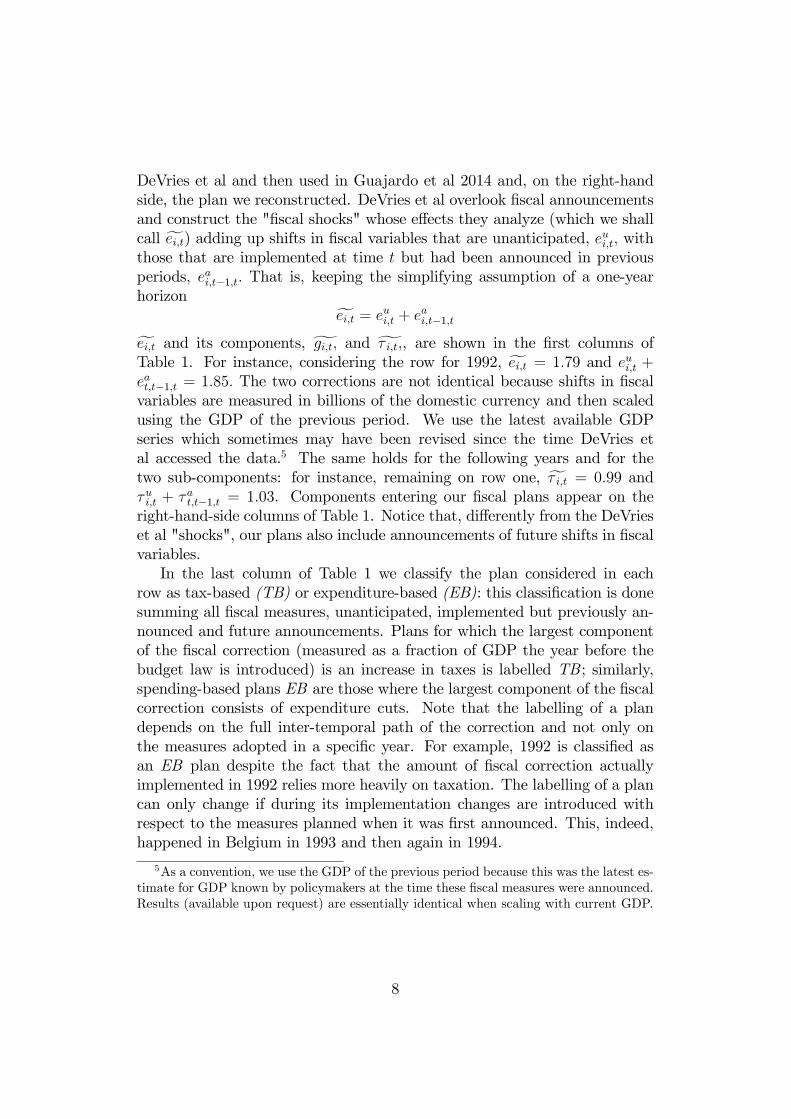
DeVries et al and then used in Guajardo et al 2014 and, on the right-handside, the plan we reconstructed. DeVries et al overlook fiscal announcementsand construct the "fiscal shocks" whose effects they analyze (which we shallcall ei,t) adding up shifts in fiscal variables that are unanticipated, eui,t, withthose that are implemented at time t but had been announced in previousperiods, eai,t−1,t. That is, keeping the simplifying assumption of a one-yearhorizon

ei,t = eui,t + eai,t−1,t

ei,t and its components, gi,t, and τ i,t,, are shown in the first columns ofTable 1. For instance, considering the row for 1992, ei,t = 1.79 and eui,t +eat,t−1,t = 1.85. The two corrections are not identical because shifts in fiscalvariables are measured in billions of the domestic currency and then scaledusing the GDP of the previous period. We use the latest available GDPseries which sometimes may have been revised since the time DeVries etal accessed the data.5 The same holds for the following years and for thetwo sub-components: for instance, remaining on row one, τ i,t = 0.99 andτui,t + τat,t−1,t = 1.03. Components entering our fiscal plans appear on theright-hand-side columns of Table 1. Notice that, differently from the DeVrieset al "shocks", our plans also include announcements of future shifts in fiscalvariables.In the last column of Table 1 we classify the plan considered in each

row as tax-based (TB) or expenditure-based (EB): this classification is donesumming all fiscal measures, unanticipated, implemented but previously an-nounced and future announcements. Plans for which the largest componentof the fiscal correction (measured as a fraction of GDP the year before thebudget law is introduced) is an increase in taxes is labelled TB ; similarly,spending-based plans EB are those where the largest component of the fiscalcorrection consists of expenditure cuts. Note that the labelling of a plandepends on the full inter-temporal path of the correction and not only onthe measures adopted in a specific year. For example, 1992 is classified asan EB plan despite the fact that the amount of fiscal correction actuallyimplemented in 1992 relies more heavily on taxation. The labelling of a plancan only change if during its implementation changes are introduced withrespect to the measures planned when it was first announced. This, indeed,happened in Belgium in 1993 and then again in 1994.

5As a convention, we use the GDP of the previous period because this was the latest es-timate for GDP known by policymakers at the time these fiscal measures were announced.Results (available upon request) are essentially identical when scaling with current GDP.

8

Table 1: Fiscal plan implemented by Belgium during 1992-1994

Year τ i,t gi,t ei,t eui,t+eat,t−1,t τui,t τai,t−1,t τai,t,t+1 gui,t gai,t−1,t gai,t,t+1 Label

1992 0.99 0.80 1.79 1.85 1.03 0 0.05 0.82 0 0.42 EB1993 0.43 0.49 0.92 0.99 0.40 0.05 0.55 0.12 0.42 0.28 TB1994 0.55 0.60 1.15 1.21 0 0.55 0 0.38 0.28 0 EB

for each year t, plans are labelled following this convention

if

(τui,t+τ

ai,t−1,t +

horiz∑j=1

τai,t,t+j

)>

(gui,t+g

ai,t−1,t +

horiz∑j=1

gai,t,t+j

)then TBi,t = 1 and EBi,t = 0, otherwise TBi,t = 0 and EBi,t = 1

To sum up. Using the narrative approach we identify consolidation episodes– that is shifts in fiscal variables extending over a number of years, and thusforming a fiscal plan – that are exogenous to output growth in the yearin which the plan is first introduced. Obviously exogeneity of the narrativeapproach is critical. We address it in the next paragraph.

2.2 The exogeneity of fiscal plans

The fact that some narratively identified fiscal adjustments are predictable,either by their own past or by past economic developments, has been consid-ered by some authors (Hernandez de Cos and Moral-Benito 2016, Jorda andTaylor 2013) a threat to their exogeneity. Here we explain why this is notthe case.Assume you overlook announcements and plans and consider instead

ei,t = eui,t + eai,t−1,t, the fiscal "shocks" analyzed by Devries et al which arefound to be predictable by their own past. As we have illustrated in theprevious section, within a plan, policy announcements are correlated withunanticipated policy shifts, that is eai,t−1,t = φ1e

ui,t−1 + v1,i,t−1. Under the null

that the eui,t are not correlated over time

Cov(ei,t, ei,t−1

)= Cov

((eui,t + eai,t−1,t

),(eui,t−1 + eai,t−2,t−1

))= Cov

((eui,t + φ1e

ui,t−1 + v1,i,t−1

),(eui,t−1 + eai,t−2,t−1

))= φ1V ar

(eui,t−1

)Finding Cov

(ei,t, ei,t−1

)6= 0 is therefore not surprising. In other words,

predictability of ei,t from their own past is a feature of multi-year fiscal plansand is properly dealt with analyzing plans rather than "shocks" such as ei,t.

9

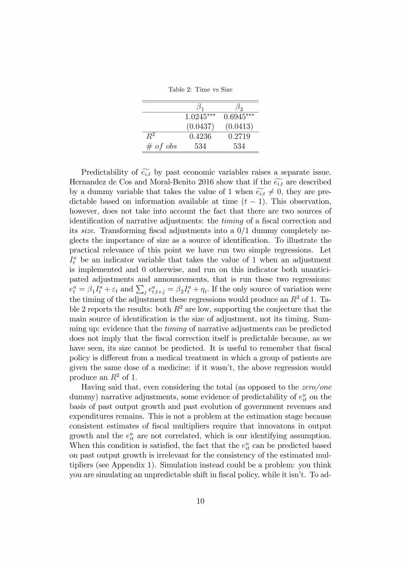
Table 2: Time vs Size

β1 β21.0245∗∗∗ 0.6945∗∗∗

(0.0437) (0.0413)R2 0.4236 0.2719# of obs 534 534

Predictability of ei,t by past economic variables raises a separate issue.Hernandez de Cos and Moral-Benito 2016 show that if the ei,t are describedby a dummy variable that takes the value of 1 when ei,t 6= 0, they are pre-dictable based on information available at time (t − 1). This observation,however, does not take into account the fact that there are two sources ofidentification of narrative adjustments: the timing of a fiscal correction andits size. Transforming fiscal adjustments into a 0/1 dummy completely ne-glects the importance of size as a source of identification. To illustrate thepractical relevance of this point we have run two simple regressions. LetIat be an indicator variable that takes the value of 1 when an adjustmentis implemented and 0 otherwise, and run on this indicator both unantici-pated adjustments and announcements, that is run these two regressions:eut = β1I

at + εt and

∑j eat,t+j = β2I

at + ηt. If the only source of variation were

the timing of the adjustment these regressions would produce an R2 of 1. Ta-ble 2 reports the results: both R2 are low, supporting the conjecture that themain source of identification is the size of adjustment, not its timing. Sum-ming up: evidence that the timing of narrative adjustments can be predicteddoes not imply that the fiscal correction itself is predictable because, as wehave seen, its size cannot be predicted. It is useful to remember that fiscalpolicy is different from a medical treatment in which a group of patients aregiven the same dose of a medicine: if it wasn’t, the above regression wouldproduce an R2 of 1.Having said that, even considering the total (as opposed to the zero/one

dummy) narrative adjustments, some evidence of predictability of euit on thebasis of past output growth and past evolution of government revenues andexpenditures remains. This is not a problem at the estimation stage becauseconsistent estimates of fiscal multipliers require that innovatons in outputgrowth and the euit are not correlated, which is our identifying assumption.When this condition is satisfied, the fact that the euit can be predicted basedon past output growth is irrelevant for the consistency of the estimated mul-tipliers (see Appendix 1). Simulation instead could be a problem: you thinkyou are simulating an unpredictable shift in fiscal policy, while it isn’t. To ad-

10

dress this potential problem we analyze fiscal plans within a panel VAR thatincludes three variables: output growth and the growth rates of revenues andexpenditures as a fraction of GDP. The estimated coeffi cients on the narra-tive adjustments in this VAR (see Appendix 1) measure the effect on outputgrowth of the component of such adjustments that is orthogonal to laggedpredictors. The estimated multipliers are thus not affected by the observedpredictability. The specification of our VAR is chosen for comparability withthe literature (in particular with Auerbach and Gorodnichenko 2012, 2013)and because it is parsimonious in terms of the included variables6.

3 Non-linear fiscal multipliers

The simplest way to assess whether multipliers depend on the state of theeconomy would be to separate fiscal consolidations initiated during an eco-nomic expansion from those that started during recessions. This procedure,however, would miss the fact that the economy can start off in one state(for instance in a recession) and then, over time, transition to another (anexpansion). For this reason we use a specification in which the economy, fol-lowing the shift in fiscal policy, can move from one state to another. We alsoallow multipliers to vary depending on the type of consolidation, tax-basedvs expenditure-based. In Section 3.1 we introduce our indicator for the stateof the economy; in Section 3.2 we present our estimation and simulationframework.

3.1 Tracking the state of economy

To describe the state of the economy you don’t want to use the state attime t, when the change in fiscal policy occurs as this might be affected bythe policy shift. One possibility would be to simply use, as a predictor ofthe state at time t, output growth the year before, or a weighted averageof output growth a few years before. Auerbach and Gorodnichenko 2012,2013 have suggested using a logistic function F (sit) (where the index i refersto the country), which smoothes the distribution of ∆yi,t−j and transformsit into a variable ranging between 0 and 1. This allows for the transition

6Limiting the dimension of the VAR to three variables only should not affect our resultsas (i) plans are identified outside the estimated VAR model and are thus independent fromits specification and (ii) the dynamic effects of plans are not truncated, differently fromwhat happens in the univariate moving-average representation adopted, for instance, byRomer and Romer (2010). Adding more structure could help the interpretation of thetotal effects —by separating direct from indirect effects —but should not matter for theirmeasurement.

11

between states of the economy to happen smoothly with F (sit) being theweight given to recessions and 1 − F (sit) the weight given to expansions.Using, as a predictor of the state at time t, the weighted average of outputgrowth over the previous two years, F (si,t) is

F (si,t) =exp(−γisi,t)

1 + exp(−γisi,t), γi > 0,

si,t =(µi,t − E

(µi,t))/σ(µi,t)

µi,t =∆yi,t−1 + ∆yi,t−2

2

where µi,t is the moving average (and σ(µi,t)its standardized version)

of output growth during the previous two years and γi are the country-specific parameters of the logistic function. For comparison with Auerbachand Gorodnichenko 2012 2013, we define an economy to be in recession ifF (si,t) > 0.8. The parameters γi are then calibrated to match actual re-cession probabilities in the countries in our sample, that is the percent-age of years in which growth is negative over the sample, which consistsof yearly data from 1979 to 2014. In other words, we calibrate γi so thatcountry i spends xi per cent of time in a recessionary regime – that is,Pr(F (si,t) > 0.8) = xi, where xi is the ratio of the number of years of nega-tive GDP growth for country i to the total number of years in the sample7

.For example, since for the US this number is 17%, in order to have

Pr(F (sUS,t) > 0.8) = 0.17, we to set γUS = 1.56. This frequency of re-cession years for the US is also consistent with the NBER Dating Committeefor a longer sample, extending back to 1946, which is 20%.8 This choiceallows us to use the same criterion for all countries in the sample, as most ofthem do not have Dating Committees. In the case of Italy, to give anotherexample, γi = 2.24 so that the country spends 22% of its time in recession:thus Pr(F (sIT,t) > 0.8 = 0.22. The γ′is obtained through this calibrationprocedure are reported in Table 3. In order to see how closely this method isable to match the data, Figure 1 compares the dynamics of F (s) – the blueline – with actual recessions (defined as years of negative per capita outputgrowth and denoted by the shaded areas) in the countries of our sample9.

7To obtain values of F (s) for the entire 1981-2014 sample we use data for output growthduring two years prior to the starting date of the estimation.

8We obtain this share by considering as years of recession those in which the number

12

Table 3: Calibration of γi

γ Avg time spent in recession γ Avg time spent in recessionAUS 1.14 14% FRA 1.59 14%AUT 1.53 14% GBR 1.43 19%BEL 1.13 14% IRL 1.68 14%CAN 1.09 17% ITA 2.24 22%DEU 1.31 17% JPN 1.65 17%DNK 1.72 19% PRT 1.60 22%ESP 1.70 25% SWE 1.92 19%FIN 4.92 22% USA 1.56 17%

3.2 A model with two sources of non-linearity

In this section we introduce a model that allows us to study, simultaneously,two non-linearities in the effect of fiscal policy: one related to the state ofthe cycle, the other to the nature of the adjustment. So far the literature hasconsidered only one source of non-linearity at a time, finding it statisticallyrelevant. The model is a Smooth Transition Panel VAR with two states:recession and expansion, and a non-linearity associated with the compositionof a fiscal plan, that is we allow multipliers to differ depending on whetherthe fiscal consolidation plan is tax-based or expenditure-based. The variablesincluded are the growth rate of per capita output (∆yi,t), the percentagechange of tax revenues as a fraction of GDP (∆τ i,t) and that of primarygovernment spending, also as a fraction of GDP (∆gi,t) (We describe thesedata and in particular the choice of our tax and expenditures variables inSection 4).

of months recorded as recessionary by the NBER is at least 3.9With F (si,t) we refer to the economic conditions prevailing at the beginning of the pe-

riod in which the consolidation is implemented. Consistently with the way we constructedour indicator, in Figure 1 we plot F (si,t+1) as a measure of the state of the cycle in periodt for comparability with actual recessions.

13

∆yi,t = (1− F (si,t))AE1 (L) zi,t−1 + F (si,t)A

R1 (L) zi,t−1 +[

1− F (si,t)F (si,t)

]′ [a′ei,t b′ei,tc′ei,t d′ei,t

] [TBi,tEBi,t

]+λ1,i + χ1,t + u1,i,t (1)

∆gi,t = (1− F (si,t))AE2 (L) zi,t−1 + F (si,t)A

R2 (L) zi,t−1 +

+β11gui,t + β12g

ai,t−1,t + λ2,i + χ2,t + u2,i,t

∆τ i,t = (1− F (si,t))AE3 (L) zi,t−1 + F (si,t)A

R3 (L) zi,t−1 +

+β21τui,t + β22τ

ai,t−1,t + λ3,i + χ3,t + u3,i,t

where zt : [∆gt,∆τ t,∆yt].

The narratively identified exogenous shifts in fiscal variables enter theestimation in two ways. In the output growth equation they enter as shiftsin ei,t; these are then interacted with the type of consolidation, TB or EB.The variable ei,t, has three components

[eui,t eai,t−j,t eai,t,t+j

]because, as

we discussed, shifts in fiscal variables can be unanticipated, announced orimplementation of previously announced measures.Differently from the output growth equation, in the following two equa-

tions we assume that the growth rates revenues and expenditures (∆gi,t and∆τ i,t) are affected only by the part of the narratively identified fiscal cor-rection which is implemented in period t: gui,t and gai,t−1,t in the equationfor expenditures and τui,t and τ

ai,t−1,t in the equation for revenues. Future

announced corrections do not directly affect the dynamics of revenues andexpenditures. In these two equations the dynamics is state dependent, butnot the effects of gui,t, g

ai,t−1,t, τ

ui,t and τ

ai,t−1,t. We also assume that both rev-

enues and expenditures respond only to their own adjustments. Finally themodel also includes unobservable VAR innovations ut: these are uninterest-ing for our analysis, in the sense that we do not need to extract from themany structural shock 10.Interacting the shifts in fiscal variables with the TB and EB dummies

allows to decompose fiscal adjustments in two orthogonal components, whichthen allows their effects to be simulated separately. This would not be pos-sible if gi,t and τ i,t were directly included in the output growth equationbecause, as already observed, exogenous shifts in taxes and spending are

10We restrict the contemporaneous response of expenditure and taxation to their owncorrections to be independent of the state of the economy. This is because the effect of thefiscal shocks in the second and third equations is mainly an accounting one and should not,in principle, be heterogeneous in different states of the cycle. Removing this restrictiondoes not alter our findings (results are available from the authors).

14

correlated. If we were to include them directly, rather than through orthog-onal plans, we could only simulate the "average" adjustment plan, that is aplan that reproduces the average correlation between changes in taxes andspending observed in the estimation sample. Thus we would no longer beable to study the heterogenous effect of fiscal adjustments based on theircomposition.In the model non-linearities with respect to the state of the economy

and with respect to the composition of a fiscal plan affect output growthboth on impact and through the dynamic response of the economy to aconsolidation plan. On impact, the possible non-linearities associated witha consolidation plan – both stemming from its composition and from thestate of the economy – are described by the coeffi cient vectors a,b, c,d inthe first equation of model (1). The statistical relevance of these asymmetriescan be assessed testing the following restrictions:

(i) a = c, b = d : the only source of non-linearity in the contemporaneouseffect of a plan arises from its type (EB vs TB);

(ii) a = b, c = d : the only source of non-linearity in the contemporaneouseffect of a plan arises from the state of the cycle;

(iii) a = b = c = d : the impact effects of the introduction of a consolidationplan depend neither on the the state of cycle nor on the type of plan.

We shall return to these tests in the Results section below.Since fiscal plans contain announcements of future shifts in taxes and

spending, in order to simulate the effect of a plan – and differently from theestimation stage where anouncements are observed – we need to keep trackof the correlation between “news innovations”and “current innovations”. Inother words, we need to construct "artificial" announcements correlated withthe unanticipated component entering a plan.11 Moreover, since fiscal plans

11Given the presence of non-linearities, impulse responses are constructed using thegeneralized method proposed by Koop et al 1996. This implies computing

I (zi,t, n, δ, It−1) = E (zi,t+n | ei,t = δ, It−1)− E (zi,t+n | ei,t = 0, It−1)

using the following steps: (i) generate a baseline simulation for all variables by solvingthe full non-linear system dynamically forward. This requires setting to zero all shocksfor a number of periods equal to the horizon up to which impulse responses are com-puted, (ii) generate an alternative simulation for all variables by considering a particularplan and then solve dynamically forward the model up to the same horizon used in thebaseline simulation, (iii) compute impulse responses to fiscal plans as the difference be-tween the simulated values in the two steps above, (iv) compute confidence intervals bybootstrapping.

15

include measures both on the tax side and on the spending side, we also needto estimate the contemporaneous correlation between these two components.Model (1) must thus be accompanied by a set of auxiliary equations

describing the response of announcements to contemporaneous correctionsand the relative weights of tax and spending measures within a plan. Weallow both correlations to be different according to the type of plan, TB vsEB. In other words, we allow for plans to have a different inter-temporal andinfra-temporal structure according to their type.12 Thus we estimate, alongwith the VAR, the following auxiliary regressions

τui,t = δTB0 eui,t∗TBi,t+δEB0 eui,t∗EBi,t+ε0,i,t

gui,t = ϑTB0 eui,t∗TBi,t+ϑEB0 e

u

i,t∗EBi,t+υυ0,i,t

τai,t,t+j = δTBj eui,t∗TBi,t+δEBj e

u

i,t∗EBi,t+εj,i,t j = 1, 2

gai,t,t+j = ϑTBj eui,t∗TBi,t+ϑEBj e

u

i,t∗EBi,t+υj,i,t j = 1, 2

where the first two equations describe the average tax (δ) and spending(ϑ) share of EB and TB plans. The next two equations describe the relationbetween unexpected shifts and those announced for years t + 1 and t + 2,differentiating between EB and TB plans. (These auxiliary regressions allowus to construct eai,t,t+j = τai,t,t+j+g

ai,t,t+j needed to simulate the output growth

equation). Table 4 shows the estimated coeffi cients

Table 4: Estimated coeffi cients in the auxiliary equations

δTB0 δTB1 δTB2 δEB0 δEB1 δEB20.7823 0.1552 0.0170 0.3918 −0.0415 0.0072

(0.0175) (0.0278) (0.0099) (0.0104) (0.0165) (0.0059)

ϑTB0 ϑTB1 ϑTB2 ϑEB0 ϑEB1 ϑEB20.2177 0.1290 0.0305 0.6082 0.1590 0.0364

(0.0175) (0.0315) (0.0152) (0.0104) (0.0187) (0.0091)

Before discussing the results, it is useful to make a few observations:

12Alternatively we could have allowed the intertemporal structure of plans to be country-rather than plan-specific (see Alesina, Favero and Giavazzi 2015a). We opted for the latterto impose restrictions in the auxiliary regressions more similar to those in the main system– i.e. coeffi cients restricted across countries and unrestricted across types of plans.

16

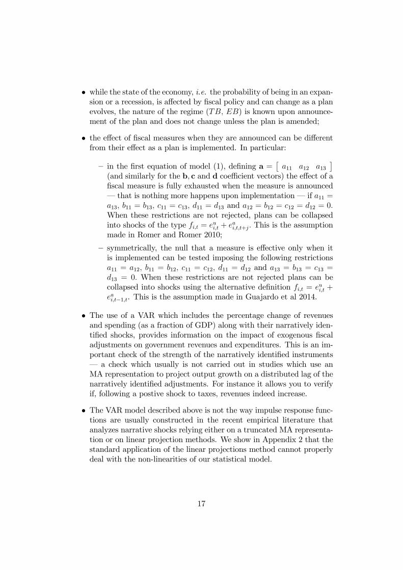
• while the state of the economy, i.e. the probability of being in an expan-sion or a recession, is affected by fiscal policy and can change as a planevolves, the nature of the regime (TB, EB) is known upon announce-ment of the plan and does not change unless the plan is amended;

• the effect of fiscal measures when they are announced can be differentfrom their effect as a plan is implemented. In particular:

— in the first equation of model (1), defining a =[a11 a12 a13

](and similarly for the b, c and d coeffi cient vectors) the effect of afiscal measure is fully exhausted when the measure is announced– that is nothing more happens upon implementation – if a11 =a13, b11 = b13, c11 = c13, d11 = d13 and a12 = b12 = c12 = d12 = 0.When these restrictions are not rejected, plans can be collapsedinto shocks of the type fi,t = eui,t + eai,t,t+j. This is the assumptionmade in Romer and Romer 2010;

— symmetrically, the null that a measure is effective only when itis implemented can be tested imposing the following restrictionsa11 = a12, b11 = b12, c11 = c12, d11 = d12 and a13 = b13 = c13 =d13 = 0. When these restrictions are not rejected plans can becollapsed into shocks using the alternative definition fi,t = eui,t +eai,t−1,t. This is the assumption made in Guajardo et al 2014.

• The use of a VAR which includes the percentage change of revenuesand spending (as a fraction of GDP) along with their narratively iden-tified shocks, provides information on the impact of exogenous fiscaladjustments on government revenues and expenditures. This is an im-portant check of the strength of the narratively identified instruments– a check which usually is not carried out in studies which use anMA representation to project output growth on a distributed lag of thenarratively identified adjustments. For instance it allows you to verifyif, following a postive shock to taxes, revenues indeed increase.

• The VAR model described above is not the way impulse response func-tions are usually constructed in the recent empirical literature thatanalyzes narrative shocks relying either on a truncated MA representa-tion or on linear projection methods. We show in Appendix 2 that thestandard application of the linear projections method cannot properlydeal with the non-linearities of our statistical model.

17

4 Data and results

4.1 Data and summary statistics

Macro data are from the OECD: Appendix 4 provides details on their sourcesand on how we compute the variables used in the analysis. Our governmentexpenditure variable is total government spending net of interest paymentson the debt: that is we do not distinguish between government consumption,government investment, transfers (Social security benefits etc) and other gov-ernment outlays. In Alesina et al 2016 we have investigated whether mul-tipliers for government transfers differ from those for other spending itemsfinding very moderate differences.Fiscal adjustment plans for the 16 countries in our sample are constructed

as described in Section 2. They are reported in Appendix 3. Tables 5 through8 illustrate the main features of our plans. Table 5 lists the number of plansthat we have identified for each country over the sample of annual data 1981-2014. A new plan is recorded whenever either a new adjustment is announcedor previously announced measures are modified. Each plan usually lasts formore than one year. We define each year of consolidation (i.e. a year inwhich we record any fiscal measure either announced or unexpected) as anepisode. Hence, every plan consists of one (if it includes only measures tobe implemented immediately) or more episodes (if it also includes announce-ments of future measures). In other words, suppose a government in year tannounces some measures to be implemented immediately and some other tobe implemented in t+ 1. If, come year t+ 1, the government just implementswhat it had previously announced, we record one plan and two episodes. Ifinstead in t + 1 it introduces some new measures, we record two plans andtwo episodes. Note that given that our data are yearly, the estimation sampleuses all the years in which there is an episode: by introducing separately, inthe estimated equations, unexpected and announced measures, we are thenable to take into account the fact that episodes build into plans.In total we have 170 plans and 216 episodes, of which about two-thirds are

EB and one-third are TB. Table 6 documents the composition of fiscal plansshowing the share of their main component, which determines the nature ofthe plan. The majority of EB (TB) plans is indeed based on spending (tax)measures. As shown in the first column of Table 6, in half of TB plans taxesaccount for 75% or more of the total adjustment and the same holds for EBones. The cases in which plans are labelled as EB or TB in the presence ofa marginally dominant component (e.g. the spending share of EB plans andthe tax share of TB ones less than 55%) are rare as shown in the last columnof Table 6.

18

Table 7 investigates whether there is a relation between the timing and thetype of fiscal adjustment and the state of the economy. Overall, adjustmentplans are more likely to be introduced during a recession. There was aconsolidation in 62 out of 99 years of recession (F (si,t) > 0.8), while werecord a consolidation in only 13 over 94 years of expansion (F (si,t) < 0.2):see the last column of Table 7. To some extent this is a consequence ofthe fact that fiscal adjustments motivated by cooling down the economy areexcluded by definition, as they are endogenous. Nevertheless, it is somewhatsurprising that a majority of the shifts in fiscal policy devoted to reducingdeficits are implemented during recessions. The relative frequency of TB andEB plans in a recession is not very different from that of the full sample. Inother words, it is not the case that EB adjustments occur more frequentlythan TB ones in a particular state of the economy (recession or expansion).For instance, of all the consolidations implemented when F (si,t) is higherthan 0.8, two-thirds were EB and one-third TB. As previously described inTable 5, these proportions hold also in our full sample.Finally, Table 8 shows the length and the size of plans. Most plans have

a one year horizon and, on average, EB plans usually last longer than TBones. The last three columns, instead, present the magnitude of, respectively,the total shift in fiscal variables, the shift corresponding to the spending sideand that corresponding to the tax side in the case of EB, TB and all newplans. EB plans are larger than TB ones and the average size of a plan is1.83% of GDP. The last two columns confirm that plans are well classifiedwith our scheme: the spending part of EB plans is larger than that of TBones and vice versa for taxes.

Table 5: Fiscal Adjustment Plans

TB EB TB EBAUS 3 4 FRA 3 7AUT 1 3 GBR 4 6BEL 4 11 IRL 6 8CAN 3 16 ITA 6 12DEU 3 6 JPN 3 5DNK 3 5 PRT 4 7ESP 8 7 SWE 0 5FIN 2 7 USA 4 4

Total TB: 57 Total EB: 113

19

Table 6: The Composition of Fiscal Adjustments

Share of Main ComponentType of Plan ≥ 0.75 < 0.75 < 0.65 < 0.55TB (57 plans) 30 27 19 9EB (113 plans) 55 58 33 7

Total Plans: 170 Total Episodes: 216

Table 7: Fiscal Adjustments and the State of the Economy

F (si,t)

Type of Plan < 0.2 < 0.5 ≥ 0.5 > 0.8TB (57 plans) 3 17 40 22EB (113 plans) 10 41 72 40

Years in Sample - (515) 94 283 232 99

Table 8: Plans’Size and Length

Horizon of plans in years Size of plans (%GDP)Type of Plan 0 1 2 3 4 5 Average Total Spending Taxes

TB 16 20 6 7 7 1 1.51 1.60 0.49 1.10EB 26 41 7 14 9 16 1.88 1.94 1.46 0.48

All Plans 42 61 13 21 16 17 1.76 1.83 1.14 0.69

4.2 Results

We first show the impulse responses from the general unrestricted modelthat allows for all non-linearities. The impulse responses of the variablesincluded in the VAR and of the indicator F (s), the probability of being ina recession regime, are presented in Figure 2. Dark blue and dark red linesshow the responses of the variables in the case, respectively, of an EB planand a TB plan introduced at a time when the economy is in an expansionarystate (defined as F (s) ' 0.2); light blue and light red lines starting froma recessionary state (defined as F (s) ' 0.8). The response of the stateindicator F (s) is computed as the difference between its simulated valuesfollowing a fiscal adjustment which starts in a recession (expansion) andits simulation in the absence of a fiscal adjustment, starting from the sameregime.

20

The upper left hand panel of Figure 2 clearly shows that the relevantnon-linearity is that between TB (red) and EB (blue) plans. In the case ofan EB consolidation, the point estimates of the responses of output growthare almost identical across the two states of the economy, while in the caseof a TB consolidation the point estimates are slightly different although thedifference is not statistically significant.The difference between EB and TB consolidations starting in any given

state of the economy is a strong feature of the data with multipliers compa-rable to those estimated in Alesina, Favero and Giavazzi 2015a abstractingfrom the state of the economy. Panels 2 and 3 of Figure 2 show the responsesof government revenues and government consumption (defined as explainedat the top of this section and both measured as a fraction of GDP) to a TBand an EB plan starting from the two initial states: expansion and recession.Importantly, revenues do indeed increase by a larger amount during a TBconsolidation, and spending decrease the most during an EB consolidation.This confirms that our classification of plans is trustworthy. Interestingly,we observe a positive (negative) response of revenues (spending) also to anEB (TB) consolidation, confirming that spending and tax measures are nottaken in isolation and thus supporting our choice of analyzing plans ratherindividual shifts in taxes and spending.Panel 4 of Figure 2 shows the responses of F (s): in all four cases a con-

solidation increases the probability of experiencing a recession (the impulseresponse is always positive). There is however a significant difference betweentype of plans. During TB consolidations F (s) increases much more than dur-ing EB ones and this holds both in expansions and recessions. Note that whena consolidation starts during a recession (cycle-down regime) the differencein F (s) is not statistically significant between Tax-based and Expenditure-based adjustment. However the total effect on output growth —which is whatmatters and is the result of the effect going through the response of F (s) aswell as the effect going through all other coeffi cients in the model —is alwaysstatistically different between the two types of adjustment.The first three rows of Table 9 report tests of the hypotheses introduced

in Section 3.2

(i) a = c, b = d : the only source of non-linearity in the contemporaneouseffect of a plan arises from its type (EB vs TB);

(ii) a = b, c = d : the only source of non-linearity in the contemporaneouseffect of a plan arises from the state of the cycle;

(iii) a = b = c = d : the impact effects of the introduction of a consolidationplan depend neither on the the state of cycle nor on the type of plan.

21

The only hypothesis that cannot be rejected is (i) i.e. the hypothesisthat the only source of non-linearity in the contemporaneous effect of a fiscaladjustment is the type of plan (EB vs TB). In the model so far, the dynamicresponse of the economy is allowed to be different during expansions (E)and recessions (R) through the auto-regressive coeffi cients, A. Assuming theresult of test (i) we have thus tested that neither the contemporaneous effectof a plan nor its dynamic response depend on the cycle, test (iv), and finallywe have tested a standard linear VAR without non-linearities. Both arerejected.(iv) AE1 (L) = AR1 (L) , AE2 (L) = AR2 (L) and AE3 (L) = AR3 (L) given

a = c, b = d: neither the contemporaneous effect of a plan nor its dynamicresponse depend on the cycle; and finally(v) a = b = c = d, AE1 (L) = AR1 (L) , AE2 (L) = AR2 (L) and AE3 (L) =

AR3 (L) we are left with a standard linear VAR model without non-linearities.

Table 9: Hypotheses’Tests

H0 Likelihood. ratio Number of Restrictions Probability(i) 6.9848 6 0.3223(ii) 16.4584 6 0.0115(iii) 20.6639 12 0.0555(iv) 26.3106 9 0.0018(v) 46.0683 21 0.0013

What these tests suggest is that the "best" model is one that restrictsthe contemporaneous effects of fiscal shocks to be equal across states of thecycle – while allowing them to differ across types of plans – and allows theautoregressive coeffi cients to be state-dependent. Figure 3 reports impulseresponses for this model. Results are quite similar to those in Figure 2. Theresponse of output is negative following the introduction of both EB and TBplans but TB consolidations are much more harmful than EB ones.In Figure 4 we remove the non-linearity across types of plans (imposing

a = b, c = d) while keeping that across states of the economy. We thus per-form an exercise that is similar to what has so far been done in the literature– with the important caveat that our estimates endogenize the state of theeconomy after a shift in fiscal policy. Looking at the first panel of the figurethe response of output after the announcement of a fiscal consolidation plandoes not appear to be affected by the state of the economy: the two impulse

22

responses are almost identical, thus confirming that the state of the economy– remember that here "state of the economy" refers to the state at the timethe consolidation is first introduced – does not seem to be relevant. In otherwords, overlooking the composition of the fiscal adjustment (TB or EB), fis-cal multipliers do not appear to differ significantly when the economy startsfrom an expansion or a recession. This result confirms the finding reportedin Ramey and Zubairy 2013, 2014, 2015. Of course this does not mean thatthe welfare effects are also similar: losing one per cent of GDP when theeconomy is already in a recession can be more harmful compared to losingthe same amount of output when the economy is expanding.The response of the indicator F (s) in the fourth panel shows that im-

plementing a consolidation always increases the probability of being in arecession – slightly more so when the economy starts from an expansionrather than a recession.Finally, in Figure 5 we keep only the non-linearity across type of plans.

In other words we replicate (using a panel VAR rather than estimating atruncated MA representation) the exercise performed in Alesina, Favero andGiavazzi 2015a. The strong similarity between the impulse responses re-ported here and those reported in our previous paper suggests that the effectof predictability of the adjustments, which is properly dealt within a VARbut not in an MA, is minor.

4.3 Robustness: evidence whenmonetary policy is con-strained

Ideally one would want to study how multipliers are affected not only by thecycle and the composition of a fiscal plan but also whether they occur at orclose to the zero lower bound. Unfortunately, we do not have enough obser-vations to consider all three factors (state of the economy, composition andZLB) together. What we can ask, however, is whether the asymmetries weidentified can be explained by a different (more or less constrained) responseof monetary policy. If the asymmetries in fiscal multipliers were related to adifferent response of monetary policy our evidence could considerably changewhen monetary policy is constrained.In order to assess the potential relevance of the monetary policy response

(or lack thereof at the ZLB) in determining the asymmetries we found above,we perform two exercises. First, we split our data in two sub-samples: euroarea countries (Austria, Belgium, France, Finland, Germany, Ireland, Italy,Portugal and Spain) from 1999 onwards and non euro-area countries (Aus-tralia, Denmark, UK, Japan, Sweden, U.S. and Canada) together with euro

23

area countries before 1999. The motivation for this split is that the commoncurrency prevents monetary policy from responding to fiscal developments inindividual member countries. However, while it is true that monetary policycannot respond at the country level, the ECB could still respond if fiscalconsolidation happened in a large enough number of euro area countries atthe same time. To capture this possible common response of monetary policyin the euro area, the specification also includes year fixed effects estimatedon euro countries from 1999 onwards. Model (1) is thus extended to

∆yi,t = (1− F (si,t))AE1 (L) zi,t−1+F (si,t)A

R1 (L) zi,t−1+

+Euroi,t ·[

1− F (si,t)F (si,t)

]′ [a′ei,t b′ei,tc′ei,t d′ei,t

] [TBi,tEBi,t

]+

+(1− Euroi,t)·[

1− F (si,t)F (si,t)

]′ [a′ei,t b′ei,tc′ei,t d′ei,t

] [TBi,tEBi,t

]+

+λi+χt · Euroi,t+∂t · (1− Euroi,t) + ui,t

with Euroi,t = 1 if

{country = AUT,BEL,DEU,ESP, FIN, FRA, IRL, ITA, PRT

year ≥ 1999

Figures 6 and 7 plot the impulse response functions from this model. Theresults appear to be similar regardless of the response of monetary policy. Theonly difference is that TB consolidations started during a recession appearto be more harmful when monetary policy is constrained. The finding thatthe response of monetary policy appears to dampen the recessionary effectsof tax-based consolidations implemented during a recession could help un-derstand the recessionary effects of European "Austerity", which was mostlytax based and implemented within a currency union.Overall, however, our results do not appear to be driven by a different

response of monetary policy to TB or EB adjustments, or to consolidationsimplemented in recession or expansion. The heterogeneity between EB andTB adjustments is in fact particularly clear when monetary policy cannot re-spond. As in the baseline simulations, there is little evidence of heterogeneityacross states of the cycle.As a further robustness check, we study whether the response of the

economy to consolidations implemented while monetary policy is at the zerolower bound plays a significant role in influencing our results. Unfortunately,we cannot split our data between countries in years at the ZLB and countriesin years out of the ZLB because the number of observations in the formergroup is too small. As an alternative we check the stability of our baselineresults by removing the observations at the ZLB from our sample, i.e. we

24

remove euro area countries in 2013 and 2014, the US from 2008 and Japanfrom 1996 onward.13 The results of this exercise are presented in Figure8. The impulse response functions are very similar to the baseline case andthis confirms that observations at the ZLB do not influence our findingssignificantly.

5 Conclusions

Fiscal consolidations can differ along three dimensions: their composition(taxes vs expenditures), the state of the business cycles (whether a consoli-dation starts in a recession or in a boom) and whether or not they occur ata ZLB or, more generally, whether monetary policy can respond to the con-solidation. In this paper we investigated the first two aspects. We concludedthat what matters for the short run output cost of fiscal consolidations is thecomposition of the adjustment. Tax-based adjustments are costly in terms ofoutput losses. Expenditure-based ones have on average very low costs: thisaverage may be the result of some cases of expansionary EB adjustments andother which are mildly recessionary. The dynamic response of the economyto a consolidation program does depend on whether this is adopted in a pe-riod of economic expansion or contraction, but the quantitative significanceof this source of non-linearity is small relative to the one which depends onthe type of consolidation. The role of the ZLB is more diffi cult to assess giventhe low number of observations. However our (admittedly not conclusive)evidence does not point towards a large difference between episodes at oraway from the ZLB, or more generally when monetary policy cannot reactto a fiscal adjustment in a monetary union. However this is an issue whichdeserves further research.13More precisely, we perform this check starting form the baseline model and interacting

the fiscal shocks in the equation for output with a dummy equal to one for observations atthe ZLB and another dummy which equals one for observations outside the ZLB. Then,we perfom our simulation using the coeffi cients estimated on the latter. We do not presentthe IRFs for consolidations at the ZLB as they are unreliable, being estimated on a verylimited number of observations.

25

6 References

Alesina, A., C. Favero and F. Giavazzi (2015a), “The output effects offiscal stabilization plans”, Journal of International Economics, 96, 1, S19-S42.Alesina A, O. Barbiero, C. Favero. F. Giavazzi and M. Paradisi (2015b),

"Austerity in 2009-13", Economic Policy.Alesina A, O. Barbiero, C. Favero. F. Giavazzi andM. Paradisi (2016),"The

output effects of fiscal adjustment plans: disaggregating taxes and spending",mimeo, IGIER.Auerbach A. and Y. Gorodnichenko (2012), “Measuring the Output Re-

sponses to Fiscal Policy”, American Economic Journal: Economic Policy,4(2), 1—27.Auerbach A. and Y. Gorodnichenko (2013), “Fiscal Multipliers in Reces-

sion and Expansion”, in A. Alesina and F. Giavazzi (eds) Fiscal Policy Afterthe Financial Crisis, 63—98, University of Chicago Press.Barnichon R. and C. Matthes (2015), "Understanding the size of Govern-

ment Spending Multipliers: it is all in the sign", mimeo CREI, UniversitatPompeu Fabra.Caggiano G., E. Castelnuovo, V. Colombo and G. Nodari (2015), "Esti-

mating Fiscal Multipliers: News from a Non-Linear World", The EconomicJournal, 125, 746-776.DeVries P., J. Guajardo, D. Leigh and A. Pescatori (2011), “A New

Action-based Dataset of Fiscal Consolidation”, IMFWorking Paper No 11/128,International Monetary Fund.Erceg, C. J. and Lindé, J (2013) “Fiscal consolidations in a currency

union: spending cuts vs. tax hikes”, Journal fo Economic Dynamics andControl, 37:2, p 422-445.Guajardo, Jaime, D. Leigh, and A. Pescatori (2014), “Expansionary Aus-

terity? International Evidence”, Journal of the European Economic Associ-ation, 12(4): 949-968.Hernandez de Cos P. and E. Moral-Benito (2016), "On the Predictability

of Narrative Fiscal Adjustments", Economics Letters, 143, 69-72Jordà, O. (2005), “Estimation and Inference of Impulse Responses by

Local Projections”, American Economic Review, 95(1): 161-182.Jordà, Ò. and A. M. Taylor (2013), "The Time for Austerity: Estimat-

ing the Average Treatment Effect of Fiscal Policy," NBER Working Papers19414, National Bureau of Economic Research, Inc.Koop G., M.H. Pesaran and S.Potter (1996), "Impulse Response Analysis

in Non-Linear Multivariate Models" Journal of Econometrics, 74, 119-147.

26

Leeper E. M., T. B. Walker and S. C. Yang (2008), “Fiscal Foresight:Analytics and Econometrics”, NBER Working Papers No. 14028, NationalBureau of Economic Research, Inc.Miyamoto, Wataru, Thuy Lan Nguyen and Dmitriy Sergeyev (2016),

"Government Spending Multipliers under the Zero Lower Bound: Evidencefrom Japan", mimeo, IGIER, Bocconi University, Milan.Ramey, V., Owyang and S. Zubairy (2013), "Are Government Spending

Multipliers Greater During Periods of Slack? Evidence from 20th CenturyHistorical Data, American Economic Review, 103(3):129-34.Ramey, Valerie A. and Sarah Zubairy (2014), "Government Spending

Multipliers in Good Times and in Bad: Evidence from U.S. Historical Data",NBER Working Paper No. 20719.Ramey, Valerie A. and Sarah Zubairy (2015), "Are Government Spending

Multipliers State Dependent? Evidence from Canadian Historical Data",mimeo.Romer C. and D. H. Romer (2010), “The Macroeconomic Effects of Tax

Changes: Estimates Based on a New Measure of Fiscal Shocks”, AmericanEconomic Review, 100(3), 763—801.

Appendix 1: Predictability and exogeneity

In a dynamic time-series model, estimation and simulation require, respec-tively, weak and strong exogeneity: these requirements are different fromlack of predictability. To illustrate the point consider the following simplifiedmodel, which only includes the unanticipated component of fiscal plans

∆yt = β0 + β1eut +

+β3∆yt−1 + β4∆τ t−1 + β5∆gt−1 + u1t

eut = γ1∆yt−1 + γ2∆τ t−1 + γ3∆gt−1 + u2t(u1tu2t

)∼ N

[(00

),

(σ11 σ12σ12 σ22

)]The condition required for eut to be weakly exogenous for the estimation of

β1 is σ12 = 0. This condition is independent of γ1, γ2, γ3. In other words, whenweak exogeneity is satisfied, the existence of predictability does not affect theconsistency of the estimate of β1. Moreover β1 measures, by construction,the impact on ∆yt of u2t, i.e. of the part of eut that cannot be predictedby ∆yt−1, ∆τ t−1 and ∆gt−1. In fact, by the partial regression theorem,when

∧u2t = eut −

∧γ1∆yt−1 +

∧γ2∆τ t−1 +

∧γ3∆gt−1 then estimating δ1 running

∆yt = δ0 + δ1∧u2t + vt, gives

∧β1 =

∧δ1.

27

Appendix 2: MA’s vs VAR’s

The VAR model described in the text (model (1)) is not the way impulseresponse functions are constructed in the recent empirical literature. In theliterature the effect of narratively identified shifts in fiscal variables relieseither on estimates of a truncated MA representation or on linear projectionmethods. The reason for these choices is that in the presence of multiple non-linearities the MA representation of a VAR is much heavier than in the linearcase – which means it could only be estimated imposing restrictions thatlimit the relevance of such non-linearities. Consider for instance the followingmodel in which fiscal adjustment plans have heterogenous effects accordingto the state of the cycle, but the VAR dynamics does not depend on thestate of the economy, that is, using the terminology in the text, AEi = ARi .Assume also that TB and EB plans have identical effects.14

zi,t = A1zi,t−1 + (1− F (si,t))B1ei,t + F (si,t)B2ei,t + ui,t (2)

where zi,t is the vector containing output growth and the growth rates oftaxes and spending, ei,t are, as in the main text, the narratively identifiedfiscal adjustments and ui,t unobservable VAR innovations. From this VARwe would derive the following MA truncated representations

zi,t =k∑j=0

Aj1 ((1− F (si,t−j))B1ei,t−j + F (si,t−j)B2ei,t−j)+k∑j=0

Aj1ui,t−j+Ak+11 zi,t−k−1

Now apply to this framework the linear projection method. This wouldamount to deriving impulse responses for the relevant component of zi,t –say ∆yi,t – running the following set of regressions15

∆yi,t+h = αi,h + (1− F (si,t))βh,1ei,t + F (si,t)βh,2ei,t + +Γhzi,t + εi,t (3)

Now compare this with the more general case in which the VAR dynamicsis also affected by the state of the cycle – that is remove the restrictionAEi = ARi , (i = 1, 2, 3)

zi,t = (1−F (si,t))A1 (L,E) zi,t−1+F (si,t)A1 (L,R) zi,t−1+(1−F (si,t))B1ei,t+F (si,t)B2ei,t+ui,t

In this case the truncated MA representation would be much more com-plicated than (3) , as the response of zi,t+h to ei,t would depend on all states

14Allowing for the presence of TB and EB plans would strengthen our point but at thecost of making the algebra more complicated.15This is the specification adopted by Auerbach and Gorodnichenko 2013 to estimate a

regime-dependent impulse response.

28

of the economy between t and t+h. Estimating the correct linear projectionwould no longer be feasible.To further illustrate the point observe that the correct linear projection

to estimate the effect of ei,t on ∆yi,t+1

∆yi,t+1 = αi,1 + (1− F (si,t+1))F (si,t)β1,1ei,t + (1− F (si,t+1))(1− F (si,t))β1,2ei,t +

+(F (si,t+1))F (si,t)β1,3ei,t + (F (si,t+1))(1− F (si,t))β1,4ei,t

+Γhzi,t + εi,t (4)

is in general different from

∆yi,t+1 = αi,h + (1− F (si,t))β1,1ei,t + F (si,t)β1,2ei,t + Γhzi,t + εi,t (5)

Note, in closing, that the cases in which the two representations coincideare very specific. Indeed, when (4) is the data generating process and (5)is estimated, the implied assumption is that the states F (si,t+1) = 1 andF (si,t+1) = 0 are observationally equivalent.Summing up: if the data are generated by (4) the VAR representation is

much more parsimonious than the linear projection which becomes practi-cally not feasible unless very strong restrictions are imposed on the empiricalmodel.

29

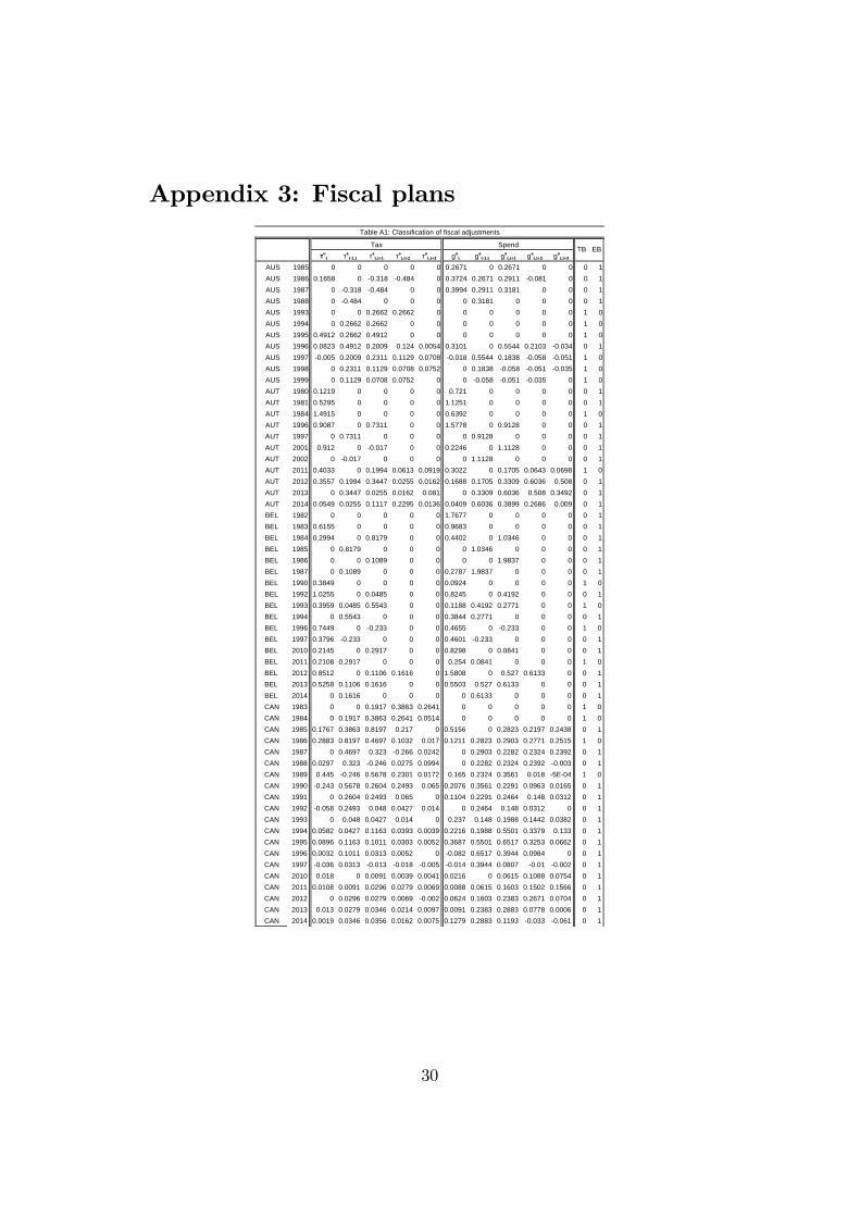
Appendix 3: Fiscal plans

τut τa

t­1,t τat,t+1 τa

t,t+2 τat,t+3 gu

t gat­1,t ga

t,t+1 gat,t+2 ga

t,t+3

AUS 1985 0 0 0 0 0 0.2671 0 0.2671 0 0 0 1AUS 1986 0.1658 0 ­0.318 ­0.484 0 0.3724 0.2671 0.2911 ­0.081 0 0 1AUS 1987 0 ­0.318 ­0.484 0 0 0.3994 0.2911 0.3181 0 0 0 1AUS 1988 0 ­0.484 0 0 0 0 0.3181 0 0 0 0 1AUS 1993 0 0 0.2662 0.2662 0 0 0 0 0 0 1 0AUS 1994 0 0.2662 0.2662 0 0 0 0 0 0 0 1 0AUS 1995 0.4912 0.2662 0.4912 0 0 0 0 0 0 0 1 0AUS 1996 0.0823 0.4912 0.2009 0.124 0.0054 0.3101 0 0.5544 0.2103 ­0.034 0 1AUS 1997 ­0.005 0.2009 0.2311 0.1129 0.0708 ­0.018 0.5544 0.1838 ­0.058 ­0.051 1 0AUS 1998 0 0.2311 0.1129 0.0708 0.0752 0 0.1838 ­0.058 ­0.051 ­0.035 1 0AUS 1999 0 0.1129 0.0708 0.0752 0 0 ­0.058 ­0.051 ­0.035 0 1 0AUT 1980 0.1219 0 0 0 0 0.721 0 0 0 0 0 1AUT 1981 0.5295 0 0 0 0 1.1251 0 0 0 0 0 1AUT 1984 1.4915 0 0 0 0 0.6392 0 0 0 0 1 0AUT 1996 0.9087 0 0.7311 0 0 1.5778 0 0.9128 0 0 0 1AUT 1997 0 0.7311 0 0 0 0 0.9128 0 0 0 0 1AUT 2001 0.912 0 ­0.017 0 0 0.2246 0 1.1128 0 0 0 1AUT 2002 0 ­0.017 0 0 0 0 1.1128 0 0 0 0 1AUT 2011 0.4033 0 0.1994 0.0613 0.0919 0.3022 0 0.1705 0.0643 0.0698 1 0AUT 2012 0.3557 0.1994 0.3447 0.0255 0.0162 0.1688 0.1705 0.3309 0.6036 0.508 0 1AUT 2013 0 0.3447 0.0255 0.0162 0.081 0 0.3309 0.6036 0.508 0.3492 0 1AUT 2014 0.0549 0.0255 0.1117 0.2295 0.0136 0.0409 0.6036 0.3899 0.2686 0.009 0 1BEL 1982 0 0 0 0 0 1.7677 0 0 0 0 0 1BEL 1983 0.6155 0 0 0 0 0.9683 0 0 0 0 0 1BEL 1984 0.2994 0 0.8179 0 0 0.4402 0 1.0346 0 0 0 1BEL 1985 0 0.8179 0 0 0 0 1.0346 0 0 0 0 1BEL 1986 0 0 0.1089 0 0 0 0 1.9837 0 0 0 1BEL 1987 0 0.1089 0 0 0 0.2787 1.9837 0 0 0 0 1BEL 1990 0.3849 0 0 0 0 0.0924 0 0 0 0 1 0BEL 1992 1.0255 0 0.0485 0 0 0.8245 0 0.4192 0 0 0 1BEL 1993 0.3959 0.0485 0.5543 0 0 0.1188 0.4192 0.2771 0 0 1 0BEL 1994 0 0.5543 0 0 0 0.3844 0.2771 0 0 0 0 1BEL 1996 0.7449 0 ­0.233 0 0 0.4655 0 ­0.233 0 0 1 0BEL 1997 0.3796 ­0.233 0 0 0 0.4601 ­0.233 0 0 0 0 1BEL 2010 0.2145 0 0.2917 0 0 0.8298 0 0.0841 0 0 0 1BEL 2011 0.2108 0.2917 0 0 0 0.254 0.0841 0 0 0 1 0BEL 2012 0.8512 0 0.1106 0.1616 0 1.5808 0 0.527 0.6133 0 0 1BEL 2013 0.5258 0.1106 0.1616 0 0 0.5503 0.527 0.6133 0 0 0 1BEL 2014 0 0.1616 0 0 0 0 0.6133 0 0 0 0 1CAN 1983 0 0 0.1917 0.3863 0.2641 0 0 0 0 0 1 0CAN 1984 0 0.1917 0.3863 0.2641 0.0514 0 0 0 0 0 1 0CAN 1985 0.1767 0.3863 0.8197 0.217 0 0.5156 0 0.2823 0.2197 0.2438 0 1CAN 1986 0.2883 0.8197 0.4697 0.1032 0.017 0.1211 0.2823 0.2903 0.2771 0.2515 1 0CAN 1987 0 0.4697 0.323 ­0.266 0.0242 0 0.2903 0.2282 0.2324 0.2392 0 1CAN 1988 0.0297 0.323 ­0.246 0.0275 0.0994 0 0.2282 0.2324 0.2392 ­0.003 0 1CAN 1989 0.445 ­0.246 0.5678 0.2301 0.0172 0.165 0.2324 0.3561 0.018 ­5E­04 1 0CAN 1990 ­0.243 0.5678 0.2604 0.2493 0.065 0.2076 0.3561 0.2291 0.0963 0.0165 0 1CAN 1991 0 0.2604 0.2493 0.065 0 0.1104 0.2291 0.2464 0.148 0.0312 0 1CAN 1992 ­0.058 0.2493 0.048 0.0427 0.014 0 0.2464 0.148 0.0312 0 0 1CAN 1993 0 0.048 0.0427 0.014 0 0.237 0.148 0.1988 0.1442 0.0382 0 1CAN 1994 0.0582 0.0427 0.1163 0.0393 0.0039 0.2216 0.1988 0.5501 0.3379 0.133 0 1CAN 1995 0.0896 0.1163 0.1011 0.0303 0.0052 0.3687 0.5501 0.6517 0.3253 0.0662 0 1CAN 1996 0.0032 0.1011 0.0313 0.0052 0 ­0.082 0.6517 0.3944 0.0984 0 0 1CAN 1997 ­0.036 0.0313 ­0.013 ­0.018 ­0.005 ­0.014 0.3944 0.0807 ­0.01 ­0.002 0 1CAN 2010 0.018 0 0.0091 0.0039 0.0041 0.0216 0 0.0615 0.1088 0.0754 0 1CAN 2011 0.0108 0.0091 0.0296 0.0279 0.0069 0.0088 0.0615 0.1603 0.1502 0.1566 0 1CAN 2012 0 0.0296 0.0279 0.0069 ­0.002 0.0624 0.1603 0.2383 0.2671 0.0704 0 1CAN 2013 0.013 0.0279 0.0346 0.0214 0.0097 0.0091 0.2383 0.2883 0.0778 0.0006 0 1CAN 2014 0.0019 0.0346 0.0356 0.0162 0.0075 0.1279 0.2883 0.1193 ­0.033 ­0.061 0 1

Table A1: Classification of fiscal adjustments

Tax Spend TB EB

30

τut τa

t­1,t τat,t+1 τa

t,t+2 τat,t+3 gu

t gat­1,t ga

t,t+1 gat,t+2 ga

t,t+3

DEU 1982 0.6343 0 0 ­0.354 0 0.7008 0 0 0 0 0 1DEU 1983 0.3467 0 ­0.354 0 0 0.6455 0 0 0 0 0 1DEU 1984 0 ­0.354 0 0 0 0.6729 0 0 0 0 0 1DEU 1991 1.1776 0 0.4114 0.1189 0.0585 0.0421 0 0.1755 0.2047 0.1852 1 0DEU 1992 0 0.4114 0.1189 0.0585 0 0 0.1755 0.2047 0.1852 0 1 0DEU 1993 0 0.1189 0.0585 0.8445 0 0 0.2047 0.1852 0.1178 0 1 0DEU 1994 0.0819 0.0585 0.9146 0 0 0.6579 0.1852 0.2611 0 0 0 1DEU 1995 0 0.9146 0 0 0 0 0.2611 0 0 0 0 1DEU 1997 0.5313 0 0 0 0 0.9935 0 ­0.08 0 0 0 1DEU 1998 0.1015 0 0 0 0 0 ­0.08 0 0 0 1 0DEU 1999 0 0 0.1313 0 0 0 0 0.5917 0 0 0 1DEU 2000 0 0.1313 0 0 ­0.381 0 0.5917 0 0 0 0 1DEU 2003 1.4821 ­0.381 ­0.68 0 0 0 0 0 0 0 1 0DEU 2004 0 ­0.68 0 0 0 1.0532 0 0 0.3039 0 0 1DEU 2005 0 0 0 0 0 0 0 0.3039 0 0 0 1DEU 2006 0 0 0.4042 0 0 0 0.3039 0.5053 0 0 0 1DEU 2007 0 0.4042 0 0 0 0 0.5053 0 0 0 0 1DEU 2011 0.3299 0 ­0.019 0 0 0.229 ­0.122 0.1263 ­0.122 0 1 0DEU 2012 ­0.074 ­0.019 ­0.193 0 0 0.5632 0.1263 ­0.033 0 0 0 1DEU 2013 0 ­0.193 0 0 0 0 ­0.033 0 0 0 0 1DNK 1982 0 0 0.1144 0 0 0 0 0 0 0 1 0DNK 1983 1.0015 0.1144 0 0 0 1.9029 0 1.2018 0 0 0 1DNK 1984 ­0.218 0 0.9084 0 0 0.763 1.2018 0.9084 0 0 0 1DNK 1985 0 0.9084 0 0 0 0 0.9084 0 0 0 0 1DNK 1994 0 0 0.0432 0 0 0 0 0 0 0 1 0DNK 1995 0 0.0432 0 0 0 0.1208 0 0 0 0 0 1DNK 2009 0 0 0 0.0975 0 0 0 0 0 0 1 0DNK 2010 0 0 0.3889 0.0971 0.4872 0 0 0.5827 0.5827 0.5827 0 1DNK 2011 0 0.3889 0.0971 0.4872 0 0 0.5827 0.5827 0.5827 0 0 1DNK 2012 0.1955 0.0971 0.585 0 0 0 0.5827 0.5827 0 0 0 1DNK 2013 0 0.585 0 0 0 0 0.5827 0 0 0 0 1ESP 1983 1.7616 0 0 0 0 0 0 0 0 0 1 0ESP 1984 0.409 0 0 0 0 0.8179 0 0 0 0 0 1ESP 1989 1.0791 0 ­0.309 0 0 0.0915 0 0 0 0 1 0ESP 1990 0 ­0.309 0 0 0 0 0 0 0 0 1 0ESP 1992 0.8245 ­0.603 0.4581 0 0 0.3665 0 0.2884 0 0 1 0ESP 1993 0.2741 0.4581 0 0 0 0 0.2884 0 0 0 1 0ESP 1994 0 0 0 0 0 1.5526 0 0 0 0 0 1ESP 1995 0 0 0 0 0 0.776 0 0 0 0 0 1ESP 1996 0.1928 0 0 0 0 1.0602 0 0 0 0 0 1ESP 1997 0.0907 0 0 0 0 1.3608 0 0 0 0 0 1ESP 2009 0.2924 0 0 0 0 0 0 0 0 0 1 0ESP 2010 0.4851 0 0 0 0 1.1695 0 0.5616 0 0 0 1ESP 2011 0 0 0 0 0 0.9807 0.5616 0 0 0 0 1ESP 2012 1.6662 0 0.8371 0 0 1.5005 0 0.4469 0.2684 0.2105 1 0ESP 2013 2.0485 0.8371 0.5853 0.2926 0 ­0.332 0.4469 0.2022 0.1337 0 1 0ESP 2014 0.9068 0.5853 0.4389 ­0.078 0 ­0.028 0.2022 0.773 0 0 1 0FIN 1992 0 0 0 0 0 0.8672 0 1.934 0 0 0 1FIN 1993 0 0 0 0 0 1.6848 1.934 0 0 0 0 1FIN 1994 1.6868 0 ­0.706 0 0 1.7653 0 0 0 0 0 1FIN 1995 0 ­0.706 0 0 0 2.4088 0 1.6028 0 0 0 1FIN 1996 0 0 ­0.273 0 0 0 1.6028 0 0 0 0 1FIN 1997 ­0.478 ­0.273 0 0 0 0.9888 0 0 0 0 0 1FIN 2010 0 0 0.6463 0.1215 0 0 0 0 0 0 1 0FIN 2011 0 0.6463 0.1215 0 0 0 0 0 0 0 1 0FIN 2012 ­0.054 0.1215 1.0331 0.0807 0.0172 0.2291 0 0.1945 0.2377 0.2581 1 0FIN 2013 0 1.0331 0.0807 0.0172 0.2438 0 0.1945 0.2377 0.2581 0 1 0FIN 2014 0 0.0807 0.2786 0.2438 0 0 0.2377 0.6962 0.0193 0.0755 0 1

Table A1: Classification of fiscal adjustments

Tax Spend TB EB

31

τut τa

t­1,t τat,t+1 τa

t,t+2 τat,t+3 gu

t gat­1,t ga

t,t+1 gat,t+2 ga

t,t+3

FRA 1979 0.9588 0 0 0 0 0 0 0 0 0 1 0FRA 1987 ­0.265 ­0.26 0 ­0.194 0 0.7502 0 0 ­0.005 0 0 1FRA 1988 0 0 ­0.194 0 0 0 0 ­0.005 0 0 0 1FRA 1989 0 ­0.194 0 0 0 0 ­0.005 0 0 0 0 1FRA 1991 0.0864 0 ­0.058 0 0 0.2188 0 0 0 0 0 1FRA 1992 0 ­0.058 0 0 0 0 0 0 0 0 0 1FRA 1995 0.4007 0 0.5067 0 0 ­0.118 0 0 0 0 1 0FRA 1996 0.4162 0.5067 0.1033 0 0 0.4012 0 0.2103 0 0 1 0FRA 1997 0.2905 0.1033 0 ­0.097 ­0.194 0 0.2103 0 0 0 0 1FRA 1998 0 0 ­0.097 ­0.194 0 0 0 0 0 0 0 1FRA 1999 0 ­0.097 ­0.194 0 0 0 0 0 0 0 0 1FRA 2000 0 ­0.194 0 0 0 0 0 0 0 0 0 1FRA 2010 0 0 0 0 0 0 0 0.3558 0 0 0 1FRA 2011 0.661 0 0.6119 0 0 0.5358 0.3558 0.5758 0.1052 0.0551 0 1FRA 2012 0.5911 0.6119 0.4409 0.01 0 0.1215 0.5758 0.1325 0.0536 0.1502 1 0FRA 2013 1.3422 0.4409 ­0.182 0 0 0.5752 0.1325 0.4371 0.1502 0.3135 0 1FRA 2014 0.1224 ­0.182 ­0.165 ­0.349 ­0.118 0.8582 0.4371 1.0823 1.0237 0.577 0 1GBR 1979 ­0.493 0 ­0.164 0 0 0.739 0 0.2463 0 0 0 1GBR 1980 0 ­0.164 0 0 0 0 0.2463 0 0 0 0 1GBR 1981 1.1107 0 0.3702 0 0 0.1234 0 0.0411 0 0 1 0GBR 1982 0 0.3702 0 0 0 0 0.0411 0 0 0 1 0GBR 1993 0 0 0.5205 0.1735 0 0 0 0 0 0 1 0GBR 1994 0.177 0.5205 0.2325 0 0 0.1261 0 0.042 0 0 1 0GBR 1995 0 0.2325 0 0 0 0 0.042 0 0 0 1 0GBR 1996 0 0 0 0 0 0.3161 0 0.1054 0 0 0 1GBR 1997 0.4633 0 0.3437 0.2398 0.0589 0.2278 0.1054 0.058 ­0.006 0 1 0GBR 1998 0 0.3437 0.2398 0.0589 0 0 0.058 ­0.006 0 0 1 0GBR 1999 0 0.2398 0.0589 0 0 0 ­0.006 0 0 0 1 0GBR 2010 0.1457 0 0.7011 0.3703 0.246 0.2629 0 0.2981 0.4054 0.4685 0 1GBR 2011 0.0462 0.7011 0.3879 0.2898 0.1448 ­0.004 0.2981 0.5252 0.7168 0.5982 0 1GBR 2012 ­0.079 0.3879 0.3135 0.2414 0.008 ­0.011 0.5252 0.7216 0.6579 0.1829 0 1GBR 2013 ­0.049 0.3135 0.3108 0.1231 ­0.043 0.0727 0.7216 0.6715 0.1608 0.0262 0 1GBR 2014 ­0.029 0.3108 0.1166 ­0.101 ­0.037 ­0.011 0.6715 0.1754 0.1172 0.0454 0 1IRL 1982 2.9483 0 0 0 0 0.3033 0 0 0 0 1 0IRL 1983 2.6459 0 0 0 0 0.0669 0 0 0 0 1 0IRL 1984 0.3127 0 0 0 0 0 0 0 0 0 1 0IRL 1985 0.1316 0 0 0 0 0 0 0 0 0 1 0IRL 1986 0.5607 0 0 0 0 0 0 0 0 0 1 0IRL 1987 0.4188 0 0 0 0 1.1986 0 0 0 0 0 1IRL 1988 0 0 0 0 0 2.0879 0 0 0 0 0 1IRL 2008 0 0 0 0 0 0 0 0.2846 0 0 0 1IRL 2009 2.8437 0 0.8922 0 0 1.2085 0.2846 0.8045 0 0 1 0IRL 2010 0.0119 0.8922 0.0315 0 0 2.4086 0.8045 0.1105 0 0 0 1IRL 2011 0.7932 0.0315 0.6245 0 0 2.5554 0.1105 0.5748 0 0 0 1IRL 2012 0.6224 0.6245 0.1311 0 0 1.327 0.5748 0.3657 0 0 0 1IRL 2013 0.6503 0.1311 0.3589 0 0 0.8829 0.3657 0.2606 0 0 0 1IRL 2014 0.1917 0.3589 ­0.034 0 0 0.7086 0.2606 0.0011 0 0 0 1ITA 1991 1.7626 0 ­1.062 0 0 0.9203 0 0 0 0 0 1ITA 1992 2.5155 ­1.062 ­1.899 0 0 1.6204 0 0 0 0 0 1ITA 1993 3.25 ­1.899 ­0.678 0 0 2.917 0 0 0 0 0 1ITA 1994 0.2575 ­0.678 0 0 0 1.5389 0 0 0 0 0 1ITA 1995 2.2616 0 ­1.515 0 0 1.6623 0 0.0565 0 0 0 1ITA 1996 1.4769 ­1.515 ­0.395 0 0 1.063 0.0565 0 0 0 0 1ITA 1997 1.2673 ­0.395 ­0.569 0 0 0.901 0 0 0 0 0 1ITA 1998 0.6162 ­0.569 0 0 0 0.567 0 0 0 0 0 1ITA 2004 0.9018 0 ­0.288 0 0 0.3449 0 0 0 0 1 0ITA 2005 0.351 ­0.288 0 0 0 0.8085 0 0 0 0 0 1ITA 2006 0.5232 0 0 0 0 0.8841 0 0 0 0 0 1ITA 2007 1.1981 0 0 0 0 ­0.36 0 0 0 0 1 0ITA 2009 0 0 0.1133 ­0.023 ­0.027 0 0 0.0075 0.0012 ­6E­04 1 0

Table A1: Classification of fiscal adjustments

Tax Spend TB EB

32

τut τa

t­1,t τat,t+1 τa

t,t+2 τat,t+3 gu

t gat­1,t ga

t,t+1 gat,t+2 ga

t,t+3

ITA 2011 0.2226 0.1754 1.2884 0.7647 0.2124 0.2335 0.6763 0.6835 0.8533 0.1503 1 0ITA 2012 0.9684 1.2884 0.7526 0.0931 0 0.3741 0.6835 1.2754 0.4812 0.0405 1 0ITA 2013 0.3141 0.7526 0.231 0.0487 0.0032 0.0372 1.2754 0.4562 0.0092 ­0.031 0 1ITA 2014 ­0.039 0.231 0.0806 0.268 0.0274 ­0.11 0.4562 0.2956 ­0.05 0.0107 1 0JPN 1979 0.1207 0 0.1399 0.0383 0 0 0 0 0 0 1 0JPN 1980 0.0901 0.1399 0.1027 0 0 0 0 0 0 0 1 0JPN 1981 0.3337 0.1027 0.2384 0 0 0 0 0 0 0 1 0JPN 1982 0.0771 0.2384 0.055 0 0 0.6842 0 0.0629 0 0 0 1JPN 1983 0 0.055 0 0 0 0.2758 0.0629 0 0 0 0 1JPN 1997 0.9816 0 0.3272 0 0 0.4395 0 0.1465 0 0 1 0JPN 1998 0 0.3272 0 0 0 0 0.1465 0 0 0 1 0JPN 2003 0 0 0 0 0 0.4884 0 0 0 0 0 1JPN 2004 0.1804 0 0.0601 0 0 0.454 0 0 0 0 0 1JPN 2005 0 0.0601 0 0 0 0.2207 0 0 0 0 0 1JPN 2006 0.4763 0 0.1588 0 0 0.2735 0 0 0 0 1 0JPN 2007 0 0.1588 0 0 0 0 0 0 0 0 1 0PRT 1983 1.0304 0 0 0 0 0.7295 0 0 0 0 1 0PRT 2000 0 0 0 0 0 0.4628 0 0 0 0 0 1PRT 2002 1.0348 0 0 0 0 0.2587 0 0 0 0 1 0PRT 2005 0.5316 0 0.4528 0 0 0.082 0 0.4765 0.9201 0 0 1PRT 2006 0.5704 0.4528 0.4916 0 0 0.786 0.4765 1.3128 0 0 0 1PRT 2007 0 0.4916 0 0 0 0.388 1.3128 0 0 0 0 1PRT 2010 0.6052 0 1.3832 0 0 0.5091 0 1.3832 0 0 1 0PRT 2011 0.4804 1.3832 0.8646 0.4804 0 0.538 1.3832 2.9782 1.345 0 0 1PRT 2012 0.3886 0.8646 2.6174 0 0 0.7771 2.9782 2.1221 0 0 0 1PRT 2013 0.3922 2.6174 ­0.392 0 0 0.0981 2.1221 0 0 0 1 0PRT 2014 0.5437 ­0.392 0.0679 0 0 1.5213 0 ­0.027 0 0 0 1SWE 1984 0.2269 0 0 0 0 0.7312 0 0 0 0 0 1SWE 1993 0.4046 0 0.1962 0 0 1.0176 0 0.7601 0 0 0 1SWE 1994 0 0.1962 0.1961 0.1121 0.0841 0 0.7601 0.2942 0.1681 0.1261 0 1SWE 1995 1.0645 0.1961 0.7208 0.5407 0.3607 1.5988 0.2942 1.0812 0.8111 0.5409 0 1SWE 1996 0 0.7208 0.5407 0.3607 0 0 1.0812 0.9492 0.6789 0.1381 0 1SWE 1997 0 0.5407 0.3607 0 0 0 0.9492 0.6789 0.1381 0 0 1SWE 1998 0 0.3607 0 0 0 0 0.6789 0.1381 0 0 0 1USA 1978 0.139 0 0 0.0815 0.8246 0 0 0 0 0 1 0USA 1979 0 0 0.0815 0.8246 0 0 0 0 0 0 1 0USA 1980 0 0.0815 0.8246 0 0 0 0 0 0 0 1 0USA 1981 ­0.311 0.8246 0 0 0 0 0 0 0 0 1 0USA 1983 0 0 0 0.1913 0.1106 0 0 0 0 0 1 0USA 1984 0 0 0.1913 0.1106 0 0 0 0 0 0 1 0USA 1985 0 0.1913 0.1106 0 0.4395 0 0 0 0 0 1 0USA 1986 0 0.1106 0 0.4395 0 0 0 0 0 0 1 0USA 1987 0 0 0.2826 0 0 0 0 0 0 0 1 0USA 1988 0.2382 0.2826 0 0 0 0.2731 0 0 0 0 1 0USA 1990 0.2263 0 0.3005 0.1944 ­0.004 0.0742 0 0.304 0.3252 0.3183 0 1USA 1991 0 0.3005 0.1944 ­0.004 0.0751 0 0.304 0.3252 0.3183 0.4808 0 1USA 1992 0 0.1944 ­0.004 0.0751 0.0265 0 0.3252 0.3183 0.4808 0.2384 0 1USA 1993 0.0929 ­0.004 0.4009 0.1764 0.0856 0.021 0.3183 0.5725 0.4036 0.3028 0 1USA 1994 0 0.4009 0.1764 0.0856 0.0612 0 0.5725 0.4036 0.3028 0.341 0 1USA 1995 0 0.1764 0.0856 0.0612 ­0.034 0 0.4036 0.3028 0.341 0.237 0 1USA 1996 0 0.0856 0.0612 ­0.034 0 0 0.3028 0.341 0.237 0 0 1USA 1997 0 0.0612 ­0.034 0 0 0 0.341 0.237 0 0 0 1USA 1998 0 ­0.034 0 0 0 0 0.237 0 0 0 0 1USA 2011 0 0 0 0 0 0.0368 0 0.142 0.1203 0.0785 0 1USA 2012 0 0 0 0 0 0 0.142 0.1203 0.0785 0.0501 0 1USA 2013 0.1732 0 0.1237 0 0 0.2642 0.1203 0.0785 0.0501 0.0434 0 1

Table A1: Classification of fiscal adjustments

Tax Spend TB EB

33

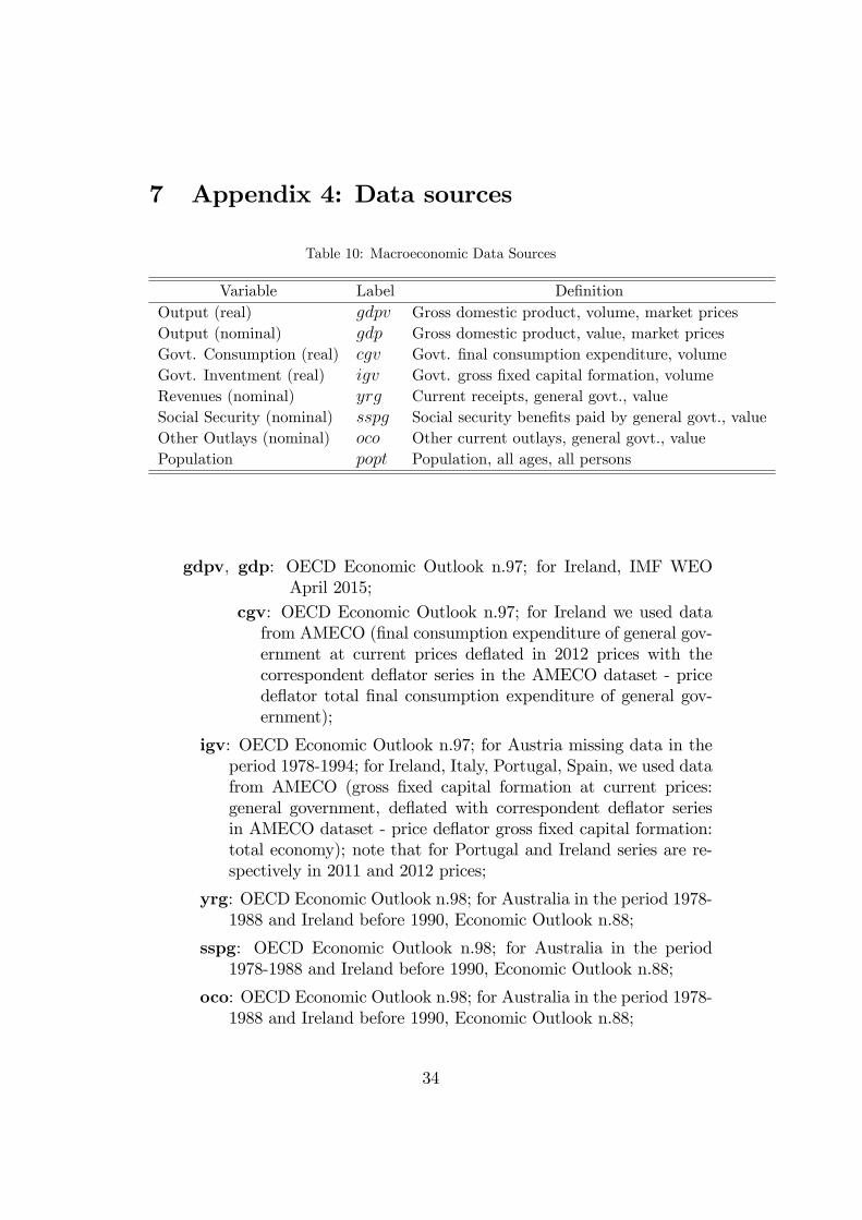
7 Appendix 4: Data sources

Table 10: Macroeconomic Data Sources

Variable Label DefinitionOutput (real) gdpv Gross domestic product, volume, market pricesOutput (nominal) gdp Gross domestic product, value, market pricesGovt. Consumption (real) cgv Govt. final consumption expenditure, volumeGovt. Inventment (real) igv Govt. gross fixed capital formation, volumeRevenues (nominal) yrg Current receipts, general govt., valueSocial Security (nominal) sspg Social security benefits paid by general govt., valueOther Outlays (nominal) oco Other current outlays, general govt., valuePopulation popt Population, all ages, all persons

gdpv, gdp: OECD Economic Outlook n.97; for Ireland, IMF WEOApril 2015;

cgv: OECD Economic Outlook n.97; for Ireland we used datafrom AMECO (final consumption expenditure of general gov-ernment at current prices deflated in 2012 prices with thecorrespondent deflator series in the AMECO dataset - pricedeflator total final consumption expenditure of general gov-ernment);

igv: OECD Economic Outlook n.97; for Austria missing data in theperiod 1978-1994; for Ireland, Italy, Portugal, Spain, we used datafrom AMECO (gross fixed capital formation at current prices:general government, deflated with correspondent deflator seriesin AMECO dataset - price deflator gross fixed capital formation:total economy); note that for Portugal and Ireland series are re-spectively in 2011 and 2012 prices;

yrg: OECD Economic Outlook n.98; for Australia in the period 1978-1988 and Ireland before 1990, Economic Outlook n.88;

sspg: OECD Economic Outlook n.98; for Australia in the period1978-1988 and Ireland before 1990, Economic Outlook n.88;

oco: OECD Economic Outlook n.98; for Australia in the period 1978-1988 and Ireland before 1990, Economic Outlook n.88;

34

popt: OECDHistorical Population Data and Projections (1950-2050).

The variables we use in the analysis are constructed as follows:

• GDP deflatorpgdpi,t =

gdpi,tgdpvi,t

• Real per capita GDP growth

∆yi,t = 100 ∗[log

(gdpvi,tgdpvi,t−1

)− log

(popti,tpopti,t−1

)]• Percentage Change of Government Spending (as fraction of GDP)

∆gi,t = 100∗[

(igvi,t + cgvi,t) +ocoi,t+sspgi,t

pgdpi,t

gdpvi,t−

(igvi,t−1 + cgvi,t−1) +ocoi,t−1+sspgi,t−1

pgdpi,t−1

gdpvi,t−1

]

• Percentage Change of Government Revenues (as fraction of GDP)

∆τ i,t = 100 ∗[ yrgi,tpgdpi,t

gdpvi,t−

yrgi,t−1pgdpi,t−1

gdpvi,t−1

]

35

Figure 1: Evolution of F (s) for the countries in our sample and years of recession (yearsnegative growth per capita, shaded areas), 1981-2013.

36

Figure 2: Allowing for heterogeneity between EB and TB plans and across states of thecycle.

Figure 3: Allowing for heterogeneity between EB and TB plans, limiting state dependenceto the autoregressive part.

37

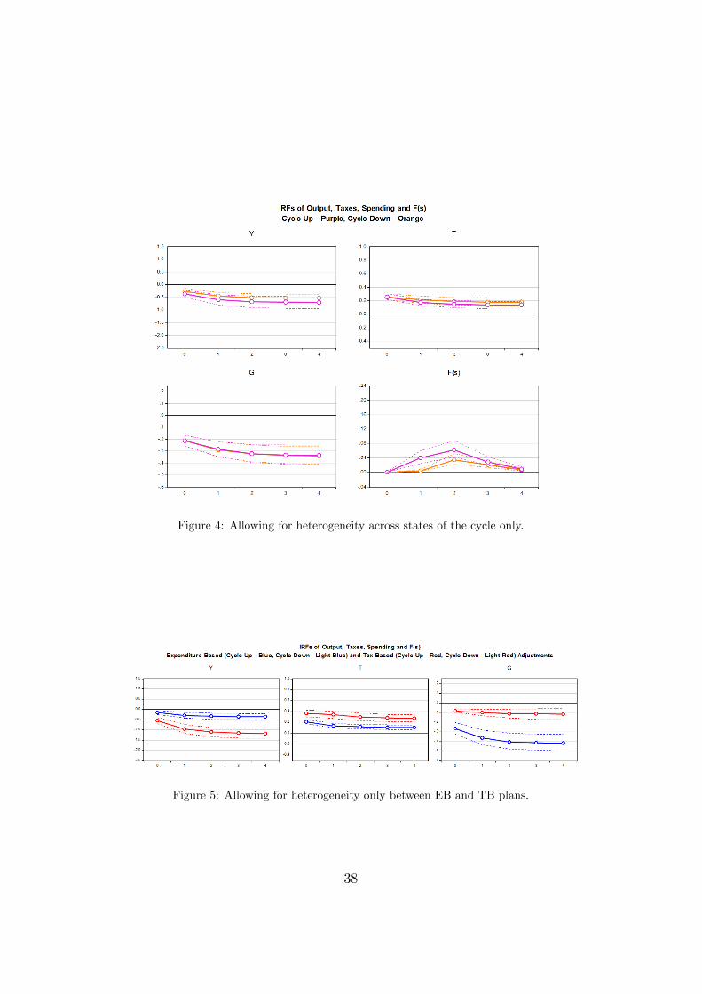
Figure 4: Allowing for heterogeneity across states of the cycle only.

Figure 5: Allowing for heterogeneity only between EB and TB plans.

38

Figure 6: Euro Area vs Non-Euro Area countries.

Figure 7: Euro Area vs Non-Euro countries.

39

Figure 8: Excluding Episodes at the ZLB.

40