Author Supervisor

Niclas Lavesson Fredrik NG Andersson

Lund University

Department of Economics

Master thesis, September 2011

Course: NEKM01

Is inflation mean-reverting?

A fractional integration approach.

Abstract

This paper investigates whether inflation series are mean-reverting. Traditional unit root tests

(ADF and KPSS tests) are conducted in the paper. These tests indicate that inflation contains

a unit root. It is however well-known that traditional unit root tests have difficulties to

distinguish between a unit root process and a fractionally integrated process (see e.g. Diebold

& Rudebusch, 1991). Hence, in this thesis, fractional integration estimators are used in order

to investigate if inflation is better modeled as a fractionally integrated process.

The main finding of this paper is that inflation with a high certainty is fractionally integrated

and mean-reverting. Another important finding is that the persistence in inflation series likely

was lower during the Bretton-Woods era relative the years after the system collapsed.

Moreover, the findings in the paper do not crucially depend on which fractional integration

estimator that are used.

Keywords: inflation, fractional integration, mean-reversion, unit root

Table of contents

1. Introduction ................................................................................................................... - 1 -

2. Estimators of the fractional integration order................................................................ - 4 -

2.1 Fractionally integrated series .................................................................................. - 4 -

2.2 Spectral estimation theory ...................................................................................... - 6 -

2.2.1 The Geweke Porter-Hudak (1983) estimator .................................................. - 7 -

2.2.2 The Robinson (1995) estimator ....................................................................... - 9 -

2.3 Wavelet estimation theory .................................................................................... - 10 -

2.3.1 Jensen’s (1999) Wavelet OLS estimator ....................................................... - 11 -

3. Data ............................................................................................................................. - 12 -

4. Analysis ....................................................................................................................... - 17 -

4.1 Traditional unit root tests ...................................................................................... - 17 -

4.2 Fractional integration estimates ............................................................................ - 20 -

5. Conclusions ................................................................................................................. - 27 -

References ................................................................................................................... - 29 -

- 1 -

1. Introduction

Inflation is often modeled as a non-stationary unit root process (see e.g. Ball & Cecchetti,

1990; Brunner & Hess, 1993; MacDonald & Murphy, 1989). If inflation contains a unit root, a

shock to the inflation series has a permanent effect (Greene, 2003). In such case, successful

inflation targeting in order to control the path of inflation is difficult to achieve for the Central

Banks (see e.g. Gregoriou & Kontonikas, 2006). To avoid misalignments from a desired

inflation level the Central Banks need appropriate policy rules. The design and

implementation of economic policy rules depends on characteristics of the inflation series

(Dias & Marques, 2010). Knowledge about the integration order and the time it takes for

inflation series to revert back to its mean value after a disturbance provides policymakers

valuable information. The purpose of this paper is therefore to investigate the statistical

properties of inflation and primarily if inflation is mean-reverting.

Since inflation is a key macroeconomic variable an increased understanding about the

inflation process is undoubtedly important. Inflation forecasts, for instance, can be improved

by an increased knowledge about the time series properties of inflation (see e.g. Hendry &

Hubrich, 2006; Hubrich, 2005). Moreover, economic frameworks are built upon assumptions

of inflation series. For instance, the long run Fisher hypothesis states that inflation and

nominal interest rates are cointegrated (Fisher, 1930). In order for variables to be cointegrated

they must have the same integration order (Greene, 2003). In Jensen (2009) it is shown that

the nominal interest rates and inflation series have different integration orders. Furthermore,

Jensen (2009) shows that inflation is mean-reverting and not a unit root process. As a

consequence, the long-run Fisher hypothesis cannot be tested (Jensen, 2009).

According to traditional integration literature a time series is modeled as either a stationary

process or simply a non-stationary unit root process (Brockwell & Davis, 2002). Fractional

integration literature provides a somewhat less restricted definition of the time series

properties (see e.g. Baillie, 1996; Granger, 1980; Granger & Joyeux, 1980; Hosking, 1981).

According to fractional integration literature a time series can take any integration order.

Hence, a time series is not restricted to be modeled as either a stationary process or a non-

stationary unit root process. For instance, a time series can be non-stationary but not

necessarily contain a unit root. Such time series is referred to as a fractionally integrated

process with long memory or simply a long memory process (Granger, 1980). The distinction

between a unit root process and a long memory process is that the latter is highly persistent

but mean-reverting in the long run. In other words, a shock eventually dissipates and the time

- 2 -

series returns to its pre-shock mean value. As a result, the Central Banks can use appropriate

economic tools to maintain price stability and thus control the inflation level to some extent.

Several papers in the past conclude that inflation is a unit root process (see e.g. Ball &

Cecchetti, 1990; Brunner & Hess, 1993; MacDonald & Murphy, 1989). A vast majority of the

studies referred to use traditional unit root tests such as the tests of Dickey-Fuller (1979),

Kwiatkowski-Phillips-Schmidt-Shin (1992), Phillips-Perron (1988) to mention some. The

conclusion that inflation is an integrated unit root process is however challenged by empirical

observations and earlier studies (see e.g. Barsky, 1987; Brimmer, 2002; Culver & Papell,

1997; Dittmar et al., 1999; Mishkin & Posen, 1997; Rose, 1988; Svensson, 1999). Findings in

Barsky (1987), Culver & Papell (1997) and Rose (1988) indicate that inflation is a stationary

process. According to Brimmer (2002) a number of Central Banks have been successful in

inflation targeting in order to control the inflation rate. Similar results as in Brimmer (2002)

are found in Mishkin & Posen (1997). Clearly, there is some evidence that Central Banks

actively can affect the inflation rate with economic policy.

The view that inflation is a unit root process can be due to shortcomings of the traditional unit

root tests as these tests do not involve the case of fractionally integrated series (see e.g.

Dickey & Fuller, 1979; Kwiatkowski et al., 1992; Phillips & Perron, 1988). Several papers

have pointed out weaknesses of the traditional unit root tests (see e.g. Blough, 1992;

Cochrane, 1991; Diebold & Rudebusch, 1991; Hassler & Wolters, 1994; Leybourne &

Newbold, 1999). The one or two most important findings in these papers are that the power

and size of traditional unit root tests are poor. The tests’ weak power implies that the

statistical tests cannot distinguish between a unit root process and a fractionally integrated

series with long memory (Baillie, 1996). As a consequence, a mean-reverting time series is

incorrectly considered as a unit root process.

Methods that involve fractionally integrated series have been used in numerous studies since

around 1980s (Baillie, 1996). For instance, Coleman (2010) investigates asymmetries in

monetary unions. According to Coleman (2010), inflation series are expected to be more

persistent in some countries of a monetary union. Therefore a common inflation shock has a

larger effect in these member countries as well. As a consequence, joint policy decisions have

different effects in each country. For similar studies as Coleman (2010), see e.g. Hofmann &

Remsperger (2005); Mooslechner & Schuerz (1999) and Batini (2006).

- 3 -

A more general result found in papers using fractional integration methods is that inflation

series for individual countries are mean-reverting (see e.g. Choudhry, 2001; Coleman, 2010;

Jensen, 2009; Zagaglia, 2009). In these studies, there are no unambiguous findings whether

inflation processes are stationary or not since this partly depends on which time period

investigated, the type of estimator used and upon the country being examined. In this paper

the main result is in accordance with findings in earlier studies since the analysis shows that

inflation likely is a mean-reverting process. Moreover, findings in the paper indicate that

inflation was less persistent during the Bretton-Woods era in comparison with the years after

the system collapsed.

In order to answer whether inflation is mean-reverting, the analysis of the paper begins with

performing traditional unit root tests. These tests are conducted to examine whether inflation

can be modeled as an integrated unit root process. The unit root tests used in the paper are the

tests of Dickey-Fuller (1979) and Kwiatkowski-Phillips-Schmidt-Shin (1992); henceforth

called the ADF and KPSS test. Next, fractional integration estimators are used to examine if

inflation is better modeled as a fractionally integrated process. Fractional integration methods

mainly operate in the frequency domain. Analyzing a time series in the frequency domain has

its advantages over traditional time series analysis. The time series of interest can be analyzed

in more detail in the frequency domain than what is possible in the time domain; cycles and

irregularities, for instance, are easier found when viewing the process in the frequency domain

(Brandes et al., 1968; Chatfield, 1996). There are a vast variety of fractional integration

estimators available and the ones used in this paper are the Geweke Porter-Hudak (1983)

estimator, Robinson (1995) estimator and Jensen’s (1999) Wavelet OLS estimator. Hereafter

called the GPH, Robinson and WOLS estimator respectively. In this paper, the countries

under investigation are Canada, Germany, Norway, Sweden, the United Kingdom and the

United States.

This study extends the existing literature by employing fractional integration methods to, in

the context, longer time series of monthly inflation data. The main contribution of the paper is

that the somewhat newly developed fractional integration methods are used when analyzing

inflation. Since the fractional integration methods are developed in later years they are not yet

widely employed. Hence, the amount of earlier research employing fractional integration

methods is rather limited. The lack of earlier research is seemingly true when considering the

WOLS estimator and analysis of the time series properties of inflation.

- 4 -

The remainder of this paper is organized as follows. In the next section, some econometric

methodology is provided. Fractionally integrated series are described and the methods used in

the paper and some properties of these are described as well. In section 3, the data material

used in the analysis is presented. Several plots over the inflation series as well as some

summary statistics are provided. Moreover, possible explanations behind the countries’

inflation patterns are discussed in section 3. The analysis of the paper is found in section 4. In

the analysis, traditional unit roots tests are conducted and the fractional integration parameter

is estimated using the fractional integration estimators. The conclusions and some discussion

about the results in the paper are found in section 5.

2. Estimators of the fractional integration order

In section 2.1 fractionally integrated series are described. An explanation of the properties of

the fractionally integrated series is provided as well. As the fractional integration estimators

mainly not operate in the time domain, theory of spectral estimation as well as wavelet

estimation are described in section 2.2 and 2.3.

The fractional integration estimators are described in the following sub-sections. In section

2.2.2 and 2.2.3 the spectral estimators (GPH and Robinson) are described. The GPH and

Robinson estimators are referred to as spectral estimators, or equivalently frequency domain

estimators, since these operate only in the frequency domain. The WOLS estimator is

described in section 2.3.1. Since the WOLS estimator operates in both the time domain and

the frequency domain it is not a pure spectral estimator. Hence, this estimator is rather

referred to as a wavelet estimator.

2.1 Fractionally integrated series

A time series is integrated of order d if the series can be represented as an invertible

autoregressive moving average (ARMA) process after being differenced d times. When d is

equal to zero the series is stationary, while d equals to one defines a non-stationary unit root

process. In the latter case, the series needs to be differenced one time (since d is equal to one)

to get an invertible ARMA representation and thus a stationary process (Brockwell & Davis,

2002).

- 5 -

In traditional unit root literature the value of d is restricted to integer values (i.e. 0 or 1).

Fractionally integrated processes can be seen as generalizations of integrated processes since

the parameter d also takes non-integer values. The simplest form of a fractional integration

process is the fractional white noise described in Granger (1980), Granger & Joyeux (1980)

and Hosking (1981) and is defined as:

(1 − �)��� = � (1)

where L is the lag operator, � is a white noise process (i.e. an independently and identically

distributed (���) process with zero mean and the variance ��) and��is a fractionally

integrated process of order d. The parameter d is the fractional integration parameter (FI-

parameter in Table 1), or equivalently the memory parameter. Properties of the fractional

integration parameter d are summarized in Table 1.

Table 1 – Properties of the fractional integration parameter (d).

Memory FI-parameter (d) Mean-reverting Variance Characteristics

No � = 0 Yes Finite Covariance stationary

Short 0 < � < 0.50 Yes Finite Covariance stationary

Long 0.50 ≤ � < 1 Yes Infinite Covariance non-stationary

Infinite � ≥ 1 No Infinite Covariance non-stationary Sources: Granger (1980); Granger & Joyeux (1980); Hosking (1981); Tkacz (2001)

A process with no memory is mean-reverting as well as finite in variance. In other words, the

process is stationary. Equation (1) reveals that stationarity occurs when the fractional

integration parameter is equal to zero. When d is equal to zero, Equation (1) translates

into�� = �. Since �by assumption is a white noise process, the time series��is a white

noise process as well when the memory parameter equals zero.

Time series with short memory has a value of the fractional integration parameter within the

interval(0 < � < 0.50). A series with short memory has the same properties as a process

with no memory except that the mean-reversion process is slower. Once a shock hits the

process, the series reverts back to the pre-shock mean value later in time. Hence, any shock

eventually dissolves when the time series has short memory.

Long memory time series differ from the stationary alternatives covered so far. The long

memory process is still stationary in its mean value and is hence mean-reverting. However,

since the fractional integration parameter lies within the span(0.50 ≤ � < 1) covariance non-

stationarity is implied (Granger, 1980; Granger & Joyeux, 1980; Hosking, 1981; Tkacz,

- 6 -

2001). The property of covariance non-stationarity arises due to the fact that the variance no

longer is finite. In all, the process reverts back to the mean level after a shock or disturbance

even if it possibly takes longer time in comparison with the no memory and short memory

time series.

The time series has the property of infinite memory when� ≥ 1. Infinite memory implies that

the series is non-stationary in both mean and variance with no tendency moving back to any

deterministic component (Tkacz, 2001). In other words, a series with infinite memory

contains a unit root. From a statistical point of view, a series with a unit root is somewhat

problematic. For instance, the variance becomes explosive as the number of observations

increases to infinity (Greene, 2003). Moreover, since a time series with infinite memory is not

mean-reverting such process randomly drifts away in any direction. To sum up, any

disturbance to a process with infinite memory is neither predictable nor transitory.

2.2 Spectral estimation theory

In pure spectral analysis, or equivalently frequency domain analysis, the time series is

expressed as frequencies in the frequency domain instead of observations in the time domain.

The different time horizons in an economy are represented by frequency bands in the

frequency domain. The long run horizon is represented by frequencies in the vicinity of the

zero frequency. Equivalently, the medium and short run of the time series such as oscillations

or business fluctuations are represented by higher frequencies (Andersson, 2008).

An orthonormal transformation is the procedure of translating a time series from one domain

into another. In frequency domain analysis the time series is translated from the time domain

into the frequency domain (Andersson, 2008). It should be possible to use an orthonormal

transformation to the transformed series as well, ending up with the original series in the

original domain (Percival & Walden, 2000). None of the statistical properties of the time

series change even though the process has been subject to an orthonormal transformation. The

mean, variance, autocovariance function and other time series properties are exactly the same

as before the transformation. The difference is that these properties are expressed in another

domain (Andersson, 2008).

When expressing a time series in the frequency domain, the orthonormal transformation is the

Fourier transformation. Basis functions in such transformation consist of sine and cosine

- 7 -

functions (Percival & Walden, 2000). Consequently, the time series is expressed as a sum of

sinusoidal components in spectral analysis:

�� = � ��� ���(��) + !� ��"(��)#$%$ �� (2)

In Equation (2), � is the frequency while ��and!� represent the amplitudes of the basis

functions at different frequencies in the interval� ∈ (−*, *). Frequencies with relatively high

values of��and!�, or in other words frequencies with large amplitudes, contribute more in

explaining the variation in the time series (Chatfield, 1996). The variance of the time series as

well can be represented in spectral terms (Andersson, 2008; Chatfield, 1996):

,�-(�) = . �/(�)��$%$ (3)

In Equation (3), the function �/(�) is called the spectral density or simply the spectrum of the

time series. This function describes how much of the variation in the time series each

frequency in the frequency interval accounts for (Chatfield, 1996). Equation (3) reveals that

all variation in the time series is covered within the frequency interval. The variance is

expressed as an integral of the spectrum in the interval� ∈ (−*, *) and since2* completes a

cycle all variation of the time series is covered.

There is a connection between the economic time horizons and the spectrum of the time

series. A large concentration of the variance around the zero frequency of the spectrum is an

indication of a long run component in the time series. Such component could be a trend

(Chatfield, 1996). A more intuitive interpretation is that frequencies concerning the long run

play a significant role in explaining the process. Similarly, a large concentration at higher

frequencies of the spectrum means that medium and short run information dominates the

process. If the frequencies in the spectrum are evenly distributed (the spectrum is flat) this

means that no time horizon dominates over another in explaining the series; thus all the time

horizons are equally important when explaining the variation of the process. Hence, when the

spectrum is flat, this corresponds to a white noise process (Baillie, 1996).

2.2.1 The Geweke Porter-Hudak (1983) estimator

The GPH estimator is built upon the spectral density of a time series (Geweke & Porter-

Hudak, 1983). Since the estimator is based on the ordinary least squares (OLS) of the log

- 8 -

spectrum, it is a spectral regression estimator. The spectrum of an economic time series is

given by:

�/(�) = 14 ��"� 3��45%���(�) (4)

In Equation (4), ��(�) is the spectral density of the white noise process � in Equation (1). As

the spectrum in Equation (4) is unknown it is estimated by the periodogram (Chatfield, 1996).

For simplicity, the terms periodogram and spectrum are used interchangeably hereafter. The

periodogram evaluated at the Fourier frequencies �6 = �$67 is denoted8(�6) for i = 1,…,m

where m denotes the number of Fourier frequencies (measured from the spectrum’s origin)

used in the OLS regression (Geweke & Porter-Hudak, 1983). T denotes the number of

observations in the time series. Taking the logarithm of 8(�6) and rewriting it as a log

periodogram regression model gives:

9�:(8(�;)) = < − � 9�: 14 ��"� 3�=�45 + >6 (5)

where>6~���(0, $@

A ) is the disturbance term (Baillie, 1996).

When running a regression on Equation (5) the estimate �BCDE is obtained. The estimate of the

memory parameter can also be obtained using the expression (see Boutahar et al., 2007):

�BCDE =F (G=%GH) IJK(L(�=))M=NOF (G=%GH)@M=NO

(6)

where PQ = − 9�: 14 ��"� 3�=�45 and PH = RS∑ P6S

6UR .

Given that the value of m is chosen correctly, the coefficient �BCDE is an estimate of the slope

of the periodogram in the vicinity of the zero frequency (Greene, 2003). The GPH estimator

utilizes that frequencies close to zero in the spectrum concern the long run horizon of the

process. Since a non-stationary process is dominated by long run information, a large estimate

of d is an indication that the time series is non-stationary. Note that this result corresponds to

what Table 1 tells. For instance, an estimate of�BCDE which is greater than or equal to one is a

strong indication that the time series is a non-stationary unit root process (infinite memory);

(see Table 1). At the other extreme, the estimated memory parameter �BCDEis zero. In such

case, the time series has no long run behavior. Or in other words, the time series has no

memory (see Table 1).

- 9 -

The choice of how many frequencies m to include in the log periodogram regression is not

straightforward. The optimal choice of m covers only the frequencies concerning the long run.

Inclusion of too many frequencies creates difficulties distinguishing between long run

behavior and the fluctuations which arise at medium and higher frequencies (Geweke &

Porter-Hudak, 1983). Moreover, the estimate �BCDE becomes biased if medium and high

frequencies are included in the estimation procedure (Geweke & Porter-Hudak, 1983).

The value of m is expressed as a function V = WX where Y = 0.50 is most commonly used

(Geweke & Porter-Hudak, 1983; Greene, 2003). Nevertheless, Y = 0.55, 0.60… 0.80 can be

used as well (see e.g. Crato & de Lima, 1994; Kumar & Okimoto, 2007). In various papers

different choices of Y works as a tool to determine the robustness of the results (see e.g.

Cheung, 1993; Choudhry, 2001).

The properties of the fractional integration parameter have been extensively examined in the

past. In a paper by Robinson (1995) an alternative estimator to the GPH estimator is

suggested.

2.2.2 The Robinson (1995) estimator

Robinson (1995) points out some shortcomings of the GPH estimator. Most importantly, it is

shown that the asymptotic properties of the GPH estimator are poor (Robinson, 1995).

Agiakloglou et al. (1993) as well as Robinson (1995) show that the GPH estimator is biased.

Robinson (1995) presents a way to lessen the extent of bias by omitting the 9 first frequencies

of the spectrum, hence yielding a consistent estimator (Boutahar et al., 2007; Robinson,

1995).

Since the intuition behind the Robinson and GPH estimator is the same, the Robinson

estimator is most easily described in the same form as Equation (6); (see Boutahar et al.,

2007):

�B]^_ =F (G=%GH) IJK�L(�=)#M=N`aOF (G=%GH)@M=N`aO

, 0 ≤ 9 < V < W (7)

where PH = RS%I∑ P6S

6UIbR and 9 corresponds to the 9 first frequencies of the spectrum.

Since there is no optimal way to choose the values of 9 and V problems can arise when

employing spectral estimators such as GPH and Robinson (Boutahar et al., 2007). However,

- 10 -

an advantage with the spectral estimators used in this paper is that the estimates follow a

normal distribution. As a consequence, standard normal theory can be used in the analysis.

2.3 Wavelet estimation theory

The major disadvantage with analysis performed exclusively in the frequency domain is that

no time resolution is considered. In the Fourier transformation, the basis functions are

periodic since sine and cosine curves are fluctuating with constant amplitude. Such functions

have no starting or ending point in time. A Fourier transformation is thus considered to be a

global transformation. As a consequence, the underlying time series must be stationary when

using the Fourier transformation (Andersson, 2008). Since economic time series rarely consist

of smooth and recurring cycles, analysis exclusively performed in the frequency domain is

often not an attractive choice for economists (Kennedy, 2008).

An alternative to spectral analysis is wavelet analysis. Wavelet analysis is not exclusively

performed in either the time domain or the frequency domain. Instead, both time and

frequency resolution are combined (Andersson, 2008). The orthonormal transform used in

wavelet analysis is the wavelet transformation. In this paper, the discrete wavelet

transformation (DWT) is of interest since inflation data is discrete. In comparison with the

Fourier transformation, there is no constraint using sine and cosine curves as basis functions

in the DWT. The basis functions in the DWT rather consist of wavelet functions (or simply

wavelets). By definition, wavelets are small waves that have a definite starting point in time.

Each wave has a certain number of oscillations and persists to a given point in time (Crowley,

2007). The property of a certain starting point and ending point in time guarantees that both

time and frequency resolution are combined in the DWT (Andersson, 2008). The DWT can be

considered as a local transformation. Hence, the underlying time series in wavelet analysis

need not to be stationary in order to achieve a valid analysis (Andersson, 2008).

The central building block when approximating a time series is the mother wavelet. The

mother wavelet is a function that takes weighted averages between neighboring observations;

simply a weighted difference operator (Crowley, 2007). In the DWT process, the mother

wavelet is used to create variants of itself to sequentially cover larger subsets of the data

material. Thus, by stretching and translating the wavelet, the complicated structure of the

process is divided into smaller less complicated components (Genҫay et al., 2002). The

translations of the wavelet function yield wavelet coefficients that are located at different

- 11 -

scales. Each scale represents a certain frequency band of the time series (Crowley, 2007).

Wavelet coefficients associated with low scales represent higher frequency behavior in the

time series, such as rapid oscillations. Higher scales represent lower frequencies of the

process (Kennedy, 2008).

The time series is represented as weighted sums of wavelets after the series has been

transformed by the DWT. The observations are modeled using contributions from every scale.

So an observation is approximated by a high frequency wavelet, a wavelet of half that

frequency, a wavelet of a quarter of the highest frequency wavelet until the lowest frequency

contribution is included (Kennedy, 2008). The strength of wavelet analysis is that the wavelet

coefficients are allowed to change depending on which time period considered. Therefore,

unusual features which have occurred at different time periods can be captured (Kennedy,

2008).

Wavelet functions exist in many different types and shapes; the Haar wavelet, Daubechies

wavelet, Mexican Hat wavelet and Morlet wavelet to mention some (see Crowley, 2007;

Genҫay et al., 2002; Percival & Walden, 2000 for further reference). Hence the choice of

mother wavelet is not straightforward and it is solely up to the researcher to determine which

type to use. However, irrespective of the wavelet type, the data sample in wavelet analysis

must be a power of two (Kennedy, 2008). This restriction on the sample size arises since the

mother wavelet is a difference operator and is translated in steps of two in the DWT.

In this paper, the simple Haar wavelet is used as well as the slightly more detailed Daubechies

(4) wavelet. However, the Haar wavelet is not considered as a good choice since it is

discontinuous and has no signs of smoothness (Crowley, 2007). A longer wavelet (i.e.

involves more observations in each translation) captures the correct frequencies better since it

is smoother (Andersson, 2008). Hence, the Daubechies (4) wavelet is used in the paper as

well. The approach using wavelets of different lengths and shapes can be considered as a

technique to check the robustness of the result (see e.g. Tkacz, 2001; Zagaglia, 2009).

2.3.1 Jensen’s (1999) Wavelet OLS estimator

Jensen (1999) proposed an estimator that can be seen as an alternative to the spectral

estimators described in the previous sections. As the name suggests, the Jensen’s WOLS is

built upon wavelet theory and OLS (see Jensen, 1999). Jensen (1999) utilizes that the variance

- 12 -

of the wavelet coefficients is a regularization of the spectrum of the time series (Percival &

Walden, 2000). When the GPH and Robinson estimators are considered, there exist a log-

linear relationship between the periodogram and the different frequencies (Geweke & Porter-

Hudak, 1983; Robinson, 1995). In a similar fashion, Jensen (1999) shows that the variance of

the wavelet coefficients is log-linearly related to the different frequency bands (scales). If the

estimated variance of the wavelet coefficientscH(d) at scale j is expressed in log terms and

rewritten into a regression model the following expression evolves:

9�: cH(d) = 9�: �� − � 9�: 2�Q + eQ (8)

where �� is the variance of the white noise process � in Equation (1) and eQ represents the

disturbance term at scale j = 1,…J where J is the highest scale.

Equation (8) is estimated using OLS. The obtained slope coefficient represents the estimate of

the fractional integration parameter�Bf^gh. An advantage with the WOLS estimator is that the

estimates of the fractional integration parameter follow a normal distribution (Jensen, 1999).

Jensen (1999) shows that the WOLS estimator is an effective and consistent estimator of the

fractional integration parameter.

3. Data

All data used in the analysis are observations of monthly CPI inflation. In the data set, the

inflation rate for the current month is calculated as the percentage change from the previous

year and corresponding month (12 month percentage change). The data for all countries,

except for the United States, originates from the OECD Statistics Database

(http://stats.oecd.org). For the United States, the data is obtained from the U.S Department of

Labor: Bureau of Labor Statistics (http://www.bls.gov/data/).

For Germany, Norway, Sweden and the United Kingdom the monthly inflation data spans

January 1956 to April 2011. For Canada there is slightly more data available since monthly

inflation data exist from January 1950. The data availability for the United States is ample.

The data material for the United States stretches over the period January 1914 until April

2011.

- 13 -

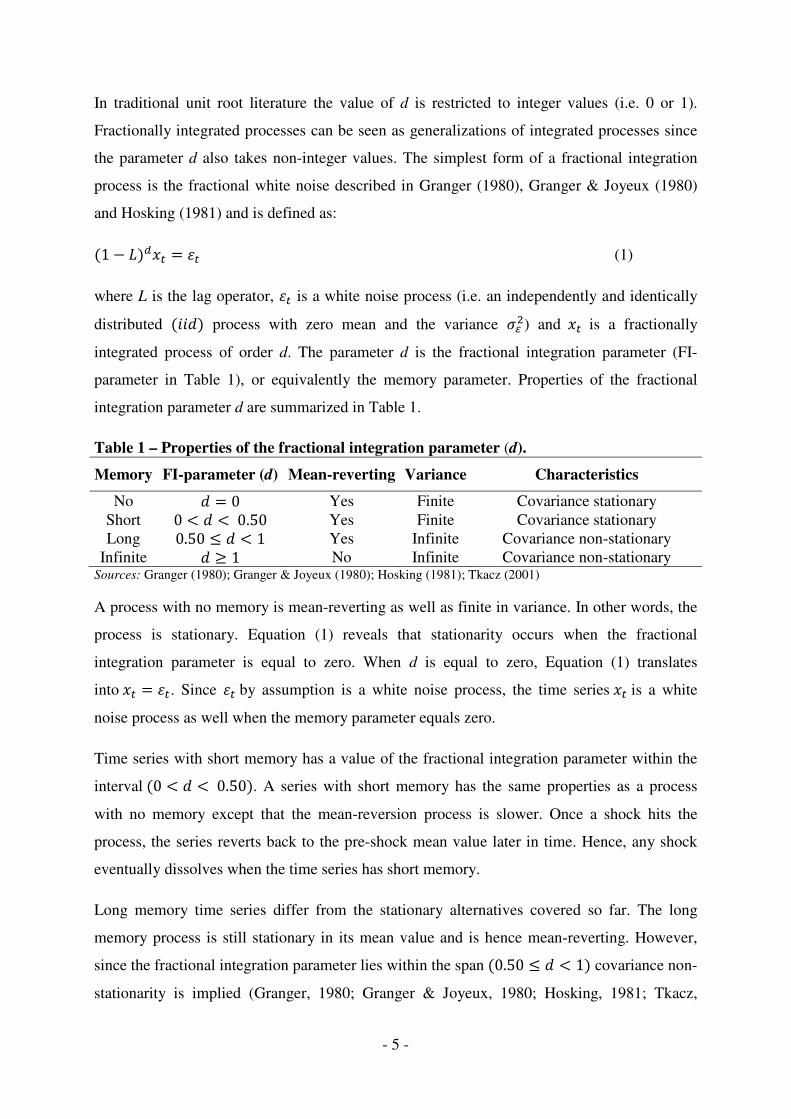
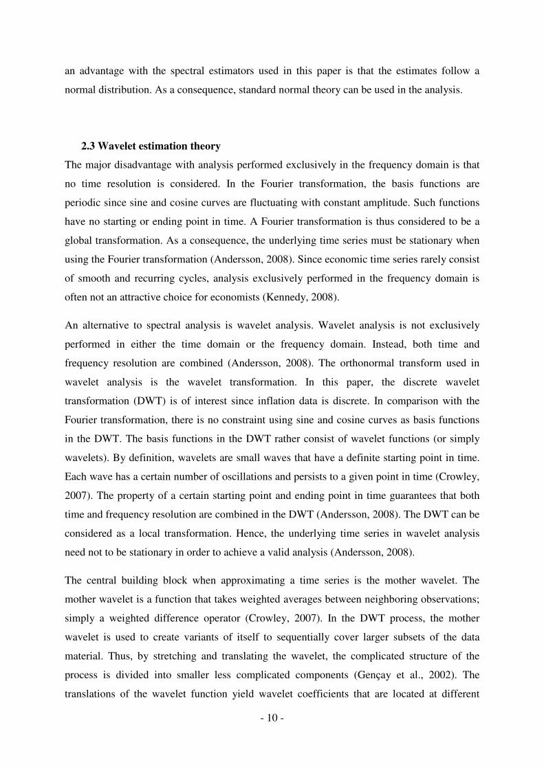
Figure 1 shows the inflation rate in the United States during 1914M1-2011M4. The variability

of the inflation rate is salient until the 1950s. This finding is expected since several crises

occurred from 1914 until the middle of 1950s. The Great Depression and the World Wars are

some major crises that can be mentioned. From the middle of 1950s until the end of the data

material in 2011M4, the inflation rate is fairly stable; an exception is the years from the

middle of 1960s until the middle of 1980s.

Figure 1: Annual inflation rates (12 month percentage change) – United States

The Vietnam War occurred 1967 and might be an explanation to why the inflation rate in the

United States increased sub-sequent years. During the 1970-1980s, the Oil Crises and the

collapse of the Bretton Woods system are possible explanations to the high inflation rates.

After year 2000, some variation in the inflation rate is seen in Figure 1. Likely, this inflation

variability is explained by fluctuations in the United States economy such as the IT boom in

the late 1990s and early 2000s as well as the financial crisis in the late 2000s.

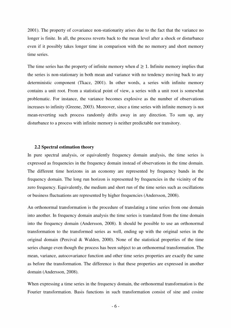
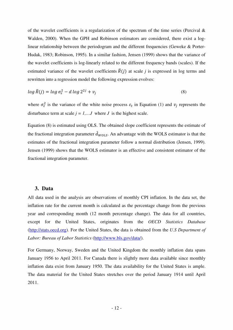
As revealed by Figure 2, a similar pattern in inflation rates as in the United States is observed

for Canada. The Canadian inflation rate is characterized by high variation in the vicinity of

the 1950s. The variable inflation rate most likely occurs due to aftereffects of the World War

II (WWII). As for the United States, the years between 1970 and 1980 are marked by high

inflation rates. Since the middle of 1990s, the Canadian inflation is fairly stable.

-20

-10

0

10

20

30

1920M01

1930M01

1940M01

1950M01

1960M01

1970M01

1980M01

1990M01

2000M01

2010M01

United States

(1914M1 - 2011M4)

Perc

en

tag

e c

han

ge (

%)

- 14 -

Figure 2: Annual inflation rates (12 month percentage change) – Canada

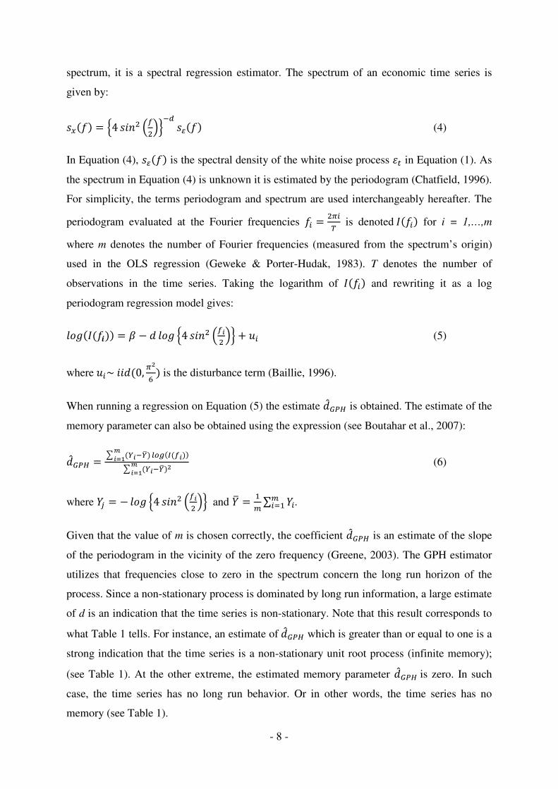
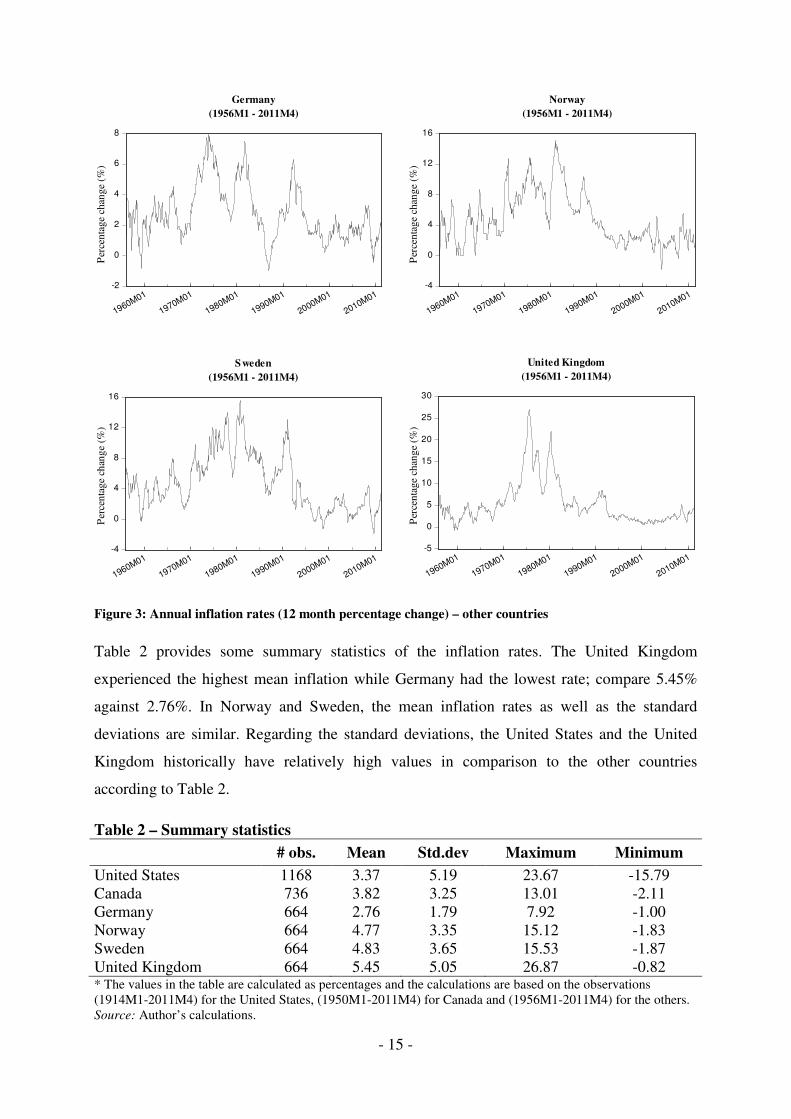
Figure 3 shows the inflation series for Germany, Norway, Sweden and the United Kingdom.

Common for these countries, is that the years around 1970s to the 1990s are characterized by

high and variable inflation. The inflation rate for the United Kingdom is fairly stable (except

during 1970-1990); such finding is not true for Germany, Norway and Sweden. In the case of

Germany, several explanations can be sought to the certain inflation pattern; possible

explanations are the aftermaths of WWII as well as the unification of East and West

Germany. Regarding Norway and Sweden, the inflation series are quite similar. A distinct

feature is the peak around 1990 in the Swedish series. The peak in inflation is probable, to

some extent, explained by the change of exchange rate regime from a pegged to a floating

system.

-4

0

4

8

12

16

1950M01

1960M01

1970M01

1980M01

1990M01

2000M01

2010M01

Canada

(1950M1 - 2011M4)P

erc

en

tag

e c

han

ge (

%)

- 15 -

Figure 3: Annual inflation rates (12 month percentage change) – other countries

Table 2 provides some summary statistics of the inflation rates. The United Kingdom

experienced the highest mean inflation while Germany had the lowest rate; compare 5.45%

against 2.76%. In Norway and Sweden, the mean inflation rates as well as the standard

deviations are similar. Regarding the standard deviations, the United States and the United

Kingdom historically have relatively high values in comparison to the other countries

according to Table 2.

Table 2 – Summary statistics

# obs. Mean Std.dev Maximum Minimum

United States 1168 3.37 5.19 23.67 -15.79

Canada 736 3.82 3.25 13.01 -2.11

Germany 664 2.76 1.79 7.92 -1.00

Norway 664 4.77 3.35 15.12 -1.83

Sweden 664 4.83 3.65 15.53 -1.87

United Kingdom 664 5.45 5.05 26.87 -0.82 * The values in the table are calculated as percentages and the calculations are based on the observations

(1914M1-2011M4) for the United States, (1950M1-2011M4) for Canada and (1956M1-2011M4) for the others.

Source: Author’s calculations.

-2

0

2

4

6

8

1960M01

1970M01

1980M01

1990M01

2000M01

2010M01

Germany

(1956M1 - 2011M4)

-4

0

4

8

12

16

1960M01

1970M01

1980M01

1990M01

2000M01

2010M01

Norway

(1956M1 - 2011M4)

-4

0

4

8

12

16

1960M01

1970M01

1980M01

1990M01

2000M01

2010M01

Sweden

(1956M1 - 2011M4)

-5

0

5

10

15

20

25

30

1960M01

1970M01

1980M01

1990M01

2000M01

2010M01

United Kingdom

(1956M1 - 2011M4)

Per

cen

tage

chan

ge

(%)

Per

cen

tag

e ch

ang

e (%

)

Per

cen

tage

chan

ge

(%)

Per

cen

tage

chan

ge

(%)

- 16 -

Table 2 reveals that the highest inflation rates occurred for the United Kingdom and the

United States. For the United Kingdom, the inflation rate reached its maximum value of

26.87% in 1975M8. The maximum inflation was 23.67% in the United States and this value

occurred in 1920M6.

Sweden, Norway and Canada historically have similar maximum inflation rates (15.53%,

15.12% and 13.01% respectively). In Sweden and Norway, the highest inflation rates

occurred 1980M10 and 1981M1 while in Canada the highest value took place in 1956M6. In

Germany, the highest inflation of 7.92% occurred 1973M12. The minimum inflation rate has

been considerably lower in the United States than in the other countries. The smallest value of

the inflation rate occurred 1921M6 and was -15.79%. For the other countries, the minimum

inflation rates are fairly the same ranging from -2.11% to -0.82%.

There are numerous explanations to why the inflation rate is highly variable and differs

between the countries. Only a few explanations have been discussed so far. Inflation

uncertainty and inflation expectations are indeed other possible explanations to certain

inflation patterns (see e.g. Ball & Cecchetti, 1990). Different inflation rates among countries

can probably be explained by economic structures as well (see e.g. Coleman, 2010).

Economies have different consumer patterns and produce different goods. For instance, a

small country with a large public sector is most likely not as affected by an oil shock as a

large and mainly manufacturing country.

It is also reasonable to believe that all of the examined countries were affected by the

breakdown of the Bretton Woods system. During the Bretton Woods era the US dollar was

convertible to gold at a fixed rate. Additionally, the member economies of the Bretton Woods

system were connected to the dollar at a fixed rate. Implicitly, all currencies were pegged to a

gold reserve (Cohen, 2001). During the years 1971-1973 the currencies of the member

economies were allowed to float independently since the US dollar lost its credibility;

eventually the Bretton Woods system disbanded in 1973M2. Consequently, a large number of

countries were forced to change their exchange rate regime at this time (Cohen, 2001).

Evidently several other explanations to the inflation patterns could be mentioned than those

already discussed. However, the inflation series of the countries in this study share some

common characteristics. Mainly, the data description shows that inflation often was high and

unstable during 1970-1980s. For some countries the high and variable rates of inflation

remained until the early 1990s as well.

- 17 -

4. Analysis

In section 4.1, traditional unit root tests are conducted to examine if inflation is modeled as an

integrated unit root process. In order to answer whether traditional unit root tests model

inflation incorrectly and foremost if inflation is a mean-reverting process, fractional

integration methods are used in section 4.2.

4.1 Traditional unit root tests

In order to avoid that the traditional unit root tests are influenced of structural breaks or

periods of instability, several sub-time periods are tested in the analysis. A natural breakpoint

is to test before and after the collapse of the Bretton Woods system in February 1973 (Cohen,

2001). The rationale of analyzing before and after February 1973 arises since many countries

changed exchange rate regime when the Bretton Woods system collapsed; hence, a structural

break occurred at this point in time.

Many unit root tests are built upon asymptotic theory and it has been shown that size

distortions often are a problem; especially in small samples. Therefore many observations are

required to obtain reliable estimates. For further reference, see e.g. Blough (1992); Cochrane

(1991) and Diebold & Rudebusch (1991). As the unit root tests require many observations the

number of sub-samples considered in the paper is limited. All countries in the study are tested

before and after the collapse of the Bretton Woods system. However, since there are many

observations of the United States inflation series, additional time periods are tested for this

country. For the United States breakpoints around the time of the WWII are considered as

well as the structural break at the time of the Bretton Woods collapse.

The result of several ADF tests is presented in Table 3. The unit root null hypothesis of the

ADF tests is in most cases not rejected at any reasonable level of significance. In the case of

the United States, the result is somewhat ambiguous since the null hypothesis can be rejected

at some times (depends on which time period tested). When considering the United States,

inclusion of a trend in the test does not affect the result considerably. The null hypothesis of a

unit root can be rejected at 10% level for Canada during the period before the collapse of the

Bretton Woods system (1950M1-1973M2). However, the unit root hypothesis is only rejected

in the ADF test with an intercept as deterministic component.

- 18 -

Table 3: ADF tests

ADF test (intercept) ADF test (intercept+trend)

Country Sample period Value Prob. Value Prob.

United States 1914M1 - 2011M4 -5.536 0.000∗∗∗ -5.559 0.000∗∗∗ 1914M1 - 1939M9 -2.403 0.142 -2.879 0.171

1914M1 - 1945M8 -2.749 0.067∗ -2.869 0.174

1945M9 - 1973M2 -4.674 0.000∗∗∗ -4.406 0.003∗∗∗ 1945M9 - 2011M4 -5.309 0.000∗∗∗ -5.223 0.000∗∗∗

1973M3 - 2011M4 -2.779 0.062∗ -3.353 0.059∗ Canada 1950M1 - 2011M4 -2.320 0.166 -2.306 0.430

1950M1 - 1973M2 -2.829 0.056∗ -3.128 0.102

1973M3 - 2011M4 -1.601 0.481 -1.830 0.688

Germany 1956M1 - 2011M4 -2.403 0.141 -2.623 0.270

1956M1 - 1973M2 -1.732 0.414 -2.397 0.380

1973M3 - 2011M4 -2.487 0.119 -2.543 0.307

Norway 1956M1 - 2011M4 -2.094 0.247 -2.423 0.367

1956M1 - 1973M2 -2.134 0.232 -3.111 0.107

1973M3 - 2011M4 -1.538 0.513 -2.711 0.233

Sweden 1956M1 - 2011M4 -1.957 0.306 -2.191 0.493

1956M1 - 1973M2 -2.042 0.269 -2.724 0.228

1973M3 - 2011M4 -1.664 0.449 -2.705 0.235

United Kingdom 1956M1 - 2011M4 -2.129 0.233 -2.310 0.428

1956M1 - 1973M2 -0.673 0.850 -2.460 0.348

1973M3 - 2011M4 -1.931 0.318 -2.212 0.481 *** 1% significance ** 5% significance * 10% significance

Source: Author’s calculations.

Note that the ADF test has the null hypothesis of a unit root in the time series (see Dickey & Fuller, 1979).

Mostly, there is a straightforward interpretation of the results from the ADF tests. In general,

when considering all countries in the study, the null hypothesis of a unit root is mostly not

rejected. Hence, the ADF tests indicate that inflation is a unit root process. Consequently, the

inflation series would not return to its mean value after an inflation shock.

To lend some credibility to the results found in Table 3 additional KPSS tests are performed.

As can be seen in Table 4 the null hypothesis of the KPSS test (that the time series is

stationary) can be rejected in most cases. As previously, when considering the ADF tests, the

result for the United States is not explicit. The result of the KPSS tests seems to depend on

which data sample that is used in the testing procedure. Regarding Canada, there are some

indications of stationarity before the Bretton Woods system collapsed. The KPSS test with

only an intercept fails to reject the null hypothesis that the Canadian inflation series is

stationary. A similar result as for Canada also holds for Norway and Sweden. The null

hypothesis cannot be rejected before the Bretton Woods system collapsed. The latter

- 19 -

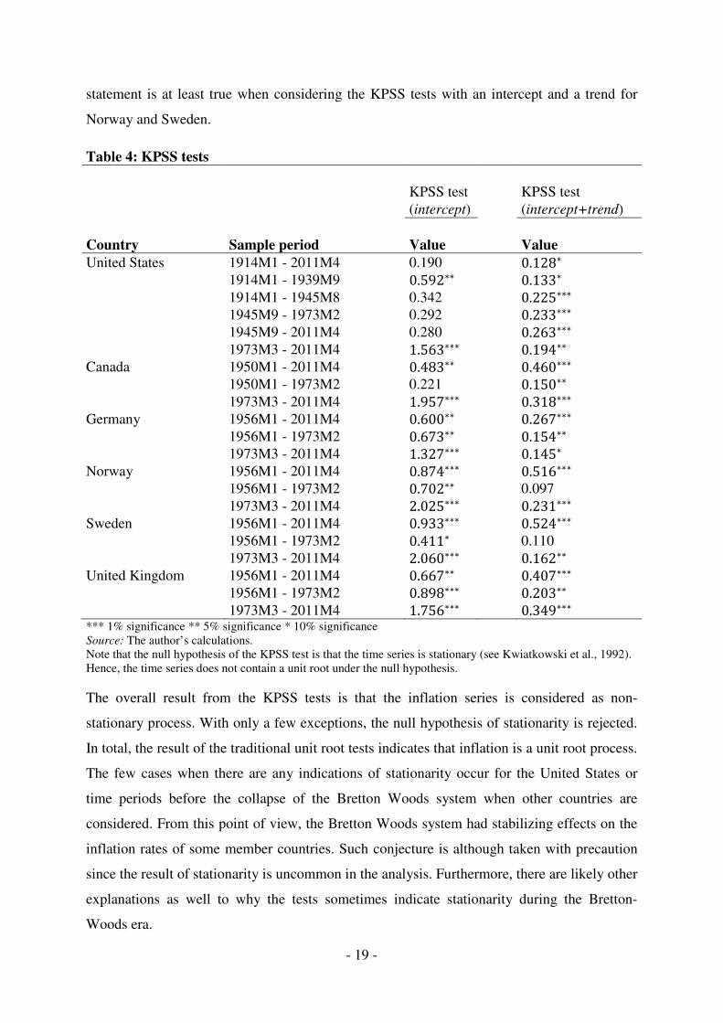
statement is at least true when considering the KPSS tests with an intercept and a trend for

Norway and Sweden.

Table 4: KPSS tests

KPSS test KPSS test

(intercept) (intercept+trend)

Country Sample period Value Value

United States 1914M1 - 2011M4 0.190 0.128∗ 1914M1 - 1939M9 0.592∗∗ 0.133∗ 1914M1 - 1945M8 0.342 0.225∗∗∗ 1945M9 - 1973M2 0.292 0.233∗∗∗ 1945M9 - 2011M4 0.280 0.263∗∗∗

1973M3 - 2011M4 1.563∗∗∗ 0.194∗∗ Canada 1950M1 - 2011M4 0.483∗∗ 0.460∗∗∗ 1950M1 - 1973M2 0.221 0.150∗∗ 1973M3 - 2011M4 1.957∗∗∗ 0.318∗∗∗ Germany 1956M1 - 2011M4 0.600∗∗ 0.267∗∗∗ 1956M1 - 1973M2 0.673∗∗ 0.154∗∗ 1973M3 - 2011M4 1.327∗∗∗ 0.145∗ Norway 1956M1 - 2011M4 0.874∗∗∗ 0.516∗∗∗

1956M1 - 1973M2 0.702∗∗ 0.097

1973M3 - 2011M4 2.025∗∗∗ 0.231∗∗∗ Sweden 1956M1 - 2011M4 0.933∗∗∗ 0.524∗∗∗

1956M1 - 1973M2 0.411∗ 0.110

1973M3 - 2011M4 2.060∗∗∗ 0.162∗∗ United Kingdom 1956M1 - 2011M4 0.667∗∗ 0.407∗∗∗

1956M1 - 1973M2 0.898∗∗∗ 0.203∗∗ 1973M3 - 2011M4 1.756∗∗∗ 0.349∗∗∗

*** 1% significance ** 5% significance * 10% significance

Source: The author’s calculations.

Note that the null hypothesis of the KPSS test is that the time series is stationary (see Kwiatkowski et al., 1992).

Hence, the time series does not contain a unit root under the null hypothesis.

The overall result from the KPSS tests is that the inflation series is considered as non-

stationary process. With only a few exceptions, the null hypothesis of stationarity is rejected.

In total, the result of the traditional unit root tests indicates that inflation is a unit root process.

The few cases when there are any indications of stationarity occur for the United States or

time periods before the collapse of the Bretton Woods system when other countries are

considered. From this point of view, the Bretton Woods system had stabilizing effects on the

inflation rates of some member countries. Such conjecture is although taken with precaution

since the result of stationarity is uncommon in the analysis. Furthermore, there are likely other

explanations as well to why the tests sometimes indicate stationarity during the Bretton-

Woods era.

- 20 -

According to the tests performed so far it is more the rule than the exception that inflation is

considered as a unit root process. The finding of a unit root in inflation is in accordance with

several other studies using similar techniques as the ones employed so far in this paper (see

e.g. Ball & Cecchetti, 1990; Brunner & Hess, 1993; MacDonald & Murphy, 1989).

4.2 Fractional integration estimates

The analysis of the fractional integration estimates begins with examining the United States

and Canada. Since there are more observations for the United States and Canada, these

countries can be analyzed more thoroughly in comparison with the other countries in the

study. In a later stage of this section, the remaining countries are examined in a similar

fashion as the United States and Canada but concerning other time periods.

The analyzed time periods differ to some extent depending on which estimator that is used in

the analysis. For the spectral estimators (GPH and Robinson) the same time periods are tested.

However, since the sample size must be a power of two when using WOLS, the analyzed time

periods differ for this estimator. Hence, the possibility to compare estimates of d between the

estimators vanishes to some extent. Such analysis is informative in order to distinguish certain

patterns during specific time periods. Since the main purpose of the paper is to investigate

whether inflation is mean-reverting, the matter of comparing different time periods is of less

importance in the paper.

Table 5 reveals that the estimates fluctuate considerably depending on the value of α. The

estimates using Wm.Amfrequencies are of less importance in the analysis since the obtained

estimates are unrealistic. Several of the estimated memory parameters in Table 5 are greater

than one. Such fractional integration orders imply an infinite and explosive variance (Greene,

2003). Series with infinite variance are characterized by an increasing variance as the number

of observations increase. An inspection of the data material in Figure 1 and Figure 2 shows no

obvious tendencies of infinite variance. Furthermore, the spectral estimates based on Y =0.60are unrealistic in comparison with the WOLS estimates as well. The value of α need not

to be specified for the WOLS estimator; hence, this estimator does not suffer from

misspecification due to an invalid choice of α.

- 21 -

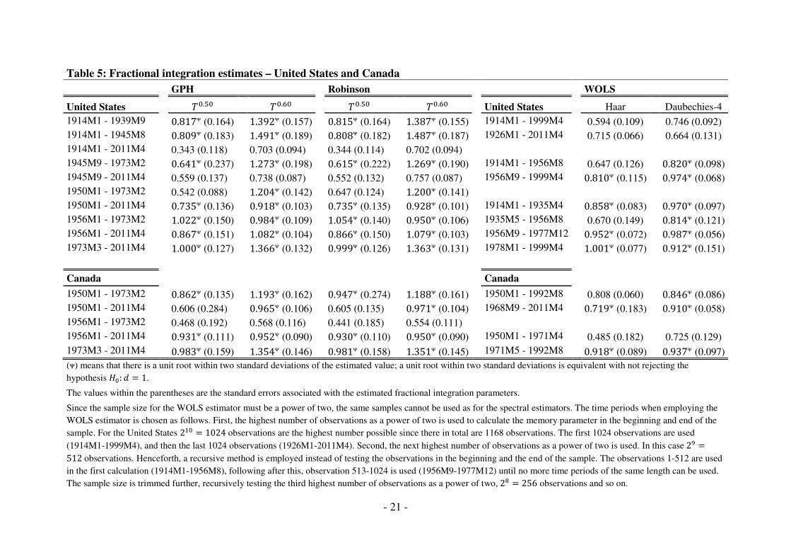
Table 5: Fractional integration estimates – United States and Canada

GPH Robinson WOLS

United States Wm.nm Wm.Am Wm.nm Wm.Am United States Haar Daubechies-4

1914M1 - 1939M9 0.817ᴪ (0.164) 1.392ᴪ (0.157) 0.815ᴪ (0.164) 1.387ᴪ (0.155) 1914M1 - 1999M4

0.594 (0.109) 0.746 (0.092)

1914M1 - 1945M8 0.809ᴪ (0.183) 1.491ᴪ (0.189) 0.808ᴪ (0.182) 1.487ᴪ (0.187) 1926M1 - 2011M4

0.715 (0.066) 0.664 (0.131)

1914M1 - 2011M4 0.343 (0.118) 0.703 (0.094) 0.344 (0.114) 0.702 (0.094)

1945M9 - 1973M2 0.641ᴪ (0.237) 1.273ᴪ (0.198) 0.615ᴪ (0.222) 1.269ᴪ (0.190) 1914M1 - 1956M8

0.647 (0.126) 0.820ᴪ (0.098)

1945M9 - 2011M4 0.559 (0.137) 0.738 (0.087) 0.552 (0.132) 0.757 (0.087) 1956M9 - 1999M4 0.810ᴪ (0.115) 0.974ᴪ (0.068)

1950M1 - 1973M2 0.542 (0.088) 1.204ᴪ (0.142) 0.647 (0.124) 1.200ᴪ (0.141)

1950M1 - 2011M4 0.735ᴪ (0.136) 0.918ᴪ (0.103) 0.735ᴪ (0.135) 0.928ᴪ (0.101) 1914M1 - 1935M4 0.858ᴪ (0.083) 0.970ᴪ (0.097)

1956M1 - 1973M2 1.022ᴪ (0.150) 0.984ᴪ (0.109) 1.054ᴪ (0.140) 0.950ᴪ (0.106) 1935M5 - 1956M8

0.670 (0.149) 0.814ᴪ (0.121)

1956M1 - 2011M4 0.867ᴪ (0.151) 1.082ᴪ (0.104) 0.866ᴪ (0.150) 1.079ᴪ (0.103) 1956M9 - 1977M12 0.952ᴪ (0.072) 0.987ᴪ (0.056)

1973M3 - 2011M4 1.000ᴪ (0.127) 1.366ᴪ (0.132) 0.999ᴪ (0.126) 1.363ᴪ (0.131) 1978M1 - 1999M4 1.001ᴪ (0.077) 0.912ᴪ (0.151)

Canada Canada

1950M1 - 1973M2 0.862ᴪ (0.135) 1.193ᴪ (0.162) 0.947ᴪ (0.274) 1.188ᴪ (0.161) 1950M1 - 1992M8

0.808 (0.060) 0.846ᴪ (0.086)

1950M1 - 2011M4 0.606 (0.284) 0.965ᴪ (0.106) 0.605 (0.135) 0.971ᴪ (0.104) 1968M9 - 2011M4 0.719ᴪ (0.183) 0.910ᴪ (0.058)

1956M1 - 1973M2 0.468 (0.192) 0.568 (0.116) 0.441 (0.185) 0.554 (0.111)

1956M1 - 2011M4 0.931ᴪ (0.111) 0.952ᴪ (0.090) 0.930ᴪ (0.110) 0.950ᴪ (0.090) 1950M1 - 1971M4

0.485 (0.182) 0.725 (0.129)

1973M3 - 2011M4 0.983ᴪ (0.159) 1.354ᴪ (0.146) 0.981ᴪ (0.158) 1.351ᴪ (0.145) 1971M5 - 1992M8 0.918ᴪ (0.089) 0.937ᴪ (0.097)

(ᴪ) means that there is a unit root within two standard deviations of the estimated value; a unit root within two standard deviations is equivalent with not rejecting the

hypothesispm: � = 1.

The values within the parentheses are the standard errors associated with the estimated fractional integration parameters.

Since the sample size for the WOLS estimator must be a power of two, the same samples cannot be used as for the spectral estimators. The time periods when employing the

WOLS estimator is chosen as follows. First, the highest number of observations as a power of two is used to calculate the memory parameter in the beginning and end of the

sample. For the United States 2Rm = 1024observations are the highest number possible since there in total are 1168 observations. The first 1024 observations are used

(1914M1-1999M4), and then the last 1024 observations (1926M1-2011M4). Second, the next highest number of observations as a power of two is used. In this case2r =512observations. Henceforth, a recursive method is employed instead of testing the observations in the beginning and the end of the sample. The observations 1-512 are used

in the first calculation (1914M1-1956M8), following after this, observation 513-1024 is used (1956M9-1977M12) until no more time periods of the same length can be used.

The sample size is trimmed further, recursively testing the third highest number of observations as a power of two,2s = 256 observations and so on.

- 22 -

In Table 5, it is examined whether a unit root is present within two standard deviations of the

estimated fractional integration parameter. Examining if a unit root exists within two standard

deviations of the estimated d is the same as testing the unit root null hypothesispm: � = 1 at

95% confidence level against the alternative hypothesispR: � < 1. Such relationship arises

since the confidence interval is the inverse of the test statistic used in hypothesis testing

(Davidson & MacKinnon, 2009).

In total, 54 relevant estimates of d are presented in Table 5 (i.e. excluding the estimates

usingWm.Am frequencies). According to Table 5, there is a unit root within two standard

deviations of the estimated value of d for 35 out of 54 of the relevant estimates. Equivalently,

the null hypothesis of a unit root is not rejected in 35 cases. From this point of view, there is

minor evidence against � = 1 since the null hypothesis seldom is rejected. However, the fact

that almost all estimates of the memory parameter in Table 5 are smaller than one (50 out of

54 estimates) is a strong indication that the true parameter value of d in fact is smaller than

one. It is reasonable to assume that the estimates of d in Table 5 are close to the true

parameter values due to unbiasedness of the estimators (the GPH estimates are likely unbiased

since these are similar to the unbiased Robinson estimates). Hence, the lack of significant

values is likely a matter of sample size rather than unreliable estimates. For instance, if very

long data samples were used significant estimates would likely occur.

Figure 1 reveals that there is a clear spike in the United States inflation series during the

WWII (1939-1945). When observations for WWII are included in the data sample, no

remarkable changes of the estimates follow. The GPH-estimate of d is 0.817 when

observations for WWII not are included in the data sample. Including observations covering

WWII as well returns an estimate of d equal to 0.809. The corresponding estimates of d for

the Robinson estimator are respectively 0.815 and 0.808.

However, the memory parameter estimates likely are affected of where and when in an

inflation cycle the data sample begins and ends. To illustrate the importance of when the

sample begins and ends, the time periods 1950M1-1973M2 and 1956M1-1973M2 for the

United States can be taken as an example. As for the years 1939-1945, the United States

inflation series during 1950-1956 is characterized by a large inflation spike (see Figure 1).

Including 1950M1-1956M1 in the estimations (i.e. using the sample 1950M1-1973M2) yields

a considerably smaller value of the estimated fractional integration parameter. Table 5 reveals

- 23 -

that the estimated fractional integration order is almost twice as large during 1956M1-

1973M2 (independent of which spectral estimator that is used).

It is difficult to draw any general conclusions about the magnitude of the fractional integration

parameter during the pre-Bretton Woods era (samples ending at 1973M2 in Table 5). Some

patterns can however be distinguished. The estimated memory parameters range from 0.468

to 1.022 when the GPH estimates are considered. The corresponding values for the Robinson

estimator are 0.441 and 1.054. Hence the estimates of d differ substantially. Several of the d

estimates are however found within the interval between 0.40 and 0.70. Values within this

span correspond to relatively low integration orders. Comparatively, the inflation series is not

highly persistent; the effect of a shock dissipates relatively fast under these circumstances,

especially for time series with a value of d that is smaller than 0.50.

The period after the Bretton Woods collapse is characterized by large estimates of the

fractional integration parameter; see the values for the United States and Canada during

1973M3-2011M4. The high fractional integration orders after 1973M2 are likely caused by

the collapse of the Bretton Woods system and the oil crises. However, other explanations can

be sought as well. For instance, in Brunner & Hess (1993) it is concluded that high levels of

inflation are less predictable. Hence, it could be the case that poor inflation forecasts caused

misaligned economic decisions which added to the effect of high and variable inflation rates.

Since the spectral estimators are sensitive to structural breaks it is difficult to draw any

general conclusion about the magnitude of d; especially when considering longer data sets.

The estimates of the memory parameter are affected since many breaks and other disturbances

occur during longer time spans. When the WOLS estimator is used structural breaks are not a

problem. In Table 5, the memory parameter estimates generated by the WOLS estimator are

almost exclusively smaller than one. The only case when the estimated d is greater than one in

Table 5 occurs for the United States in 1978M1-1999M4. Since the wavelet estimator not

heavily depend on the data samples and structural breaks, the WOLS estimates of d can be

considered as more appropriate than the spectral estimates. The overall result of the WOLS

estimates for the United States and Canada is that inflation likely is mean-reverting. Only one

out of 24 WOLS estimates in Table 5 is greater than or equal to one. In all, the estimates of d

are between 0.60 and 0.95.

Some certain patterns can be discerned when the different time periods are compared with

each other. Nearly all of the estimated memory parameters for time periods ending in 1973M2

- 24 -

are smaller than memory estimates obtained from the sample 1973M3-2011M4. This result is

true both for the United States and Canada. A similar result is seen when the WOLS estimates

are considered. Samples ending in the vicinity of the Bretton Woods collapse yield smaller

estimates of d than the corresponding estimates based on data after the collapse. More

generally, the WOLS estimates based on observations early in the data material are smaller

than the estimates obtained when using observations in the end of the data material. This

result indicates that inflation seems to be less persistent in the beginning of the data material.

In Table 6, the estimates of the fractional integration parameter for the remaining countries in

the study are found. As before the estimates using Wm.Amfrequencies are excluded from the

analysis since unrealistic estimates appear due to an invalid choice of α. In total, 56 relevant

estimates of d are available in Table 6. Six of 56 estimated values of d are greater than or

equal to one. So, the estimates of the memory parameter are mostly smaller than one and thus

the inflation series are considered as mean-reverting. Just as when analyzing the United States

and Canada, only a few of the d estimates are significantly different from one. By the same

rationale as before an increased sample size would likely create significant estimates.

Considering the spectral estimates of d before the collapse of the Bretton Woods system, the

inflation series for Germany, Sweden and the United Kingdom have the characteristics of d

being between 0.80 and 0.90. Norway has a slightly different property since the estimated

memory parameter is slightly smaller(� ≈ 0.60). Due to the plots of the time series in Figure

3, the similar values of d are expected. The inflation series for Germany, Norway, Sweden

and the United Kingdom are alike during 1956M1-1973M2.

The post Bretton Woods era 1973M3-2011M4 for the countries in Table 6 is characterized by

somewhat large spread in the estimates of the fractional integration parameter. The estimate

of d for Germany is greater than one, irrespective of which spectral estimator considered. In

the case of the United Kingdom, the estimate of d is slightly smaller than one, no matter if the

GPH or Robinson estimator is used. Norway and Sweden are similar in the sense that the

estimated memory parameters take values between 0.80 and 0.90. Figure 3 shows that the

inflation series for the latter countries are quite similar. In addition, Table 2 shows that the

inflation processes for Norway and Sweden share the same characteristics with respect to the

mean inflation rate, standard deviations and maximum/minimum values in inflation. The

result that the estimated memory parameters not differ to any greater extent between Norway

and Sweden is hence expected.

- 25 -

Table 6: Fractional integration estimates – other countries

GPH Robinson WOLS

Germany Wm.nm Wm.Am Wm.nm Wm.Am Germany Haar

Daubechies-4

1956M1 - 2011M4

0.828ᴪ (0.142) 0.881ᴪ (0.112)

0.823ᴪ (0.131) 0.837ᴪ (0.112)

1956M1 - 1998M8 0.648 (0.119)

0.816 (0.051) 1956M1 - 1973M2

0.850ᴪ (0.115) 0.969ᴪ (0.092)

0.850ᴪ (0.115) 0.967ᴪ (0.092)

1968M9 - 2011M4 0.834 (0.062) 0.880ᴪ (0.072)

1973M3 - 2011M4

1.035ᴪ (0.233) 1.035ᴪ (0.233)

1.034ᴪ (0.233) 1.034ᴪ (0.233)

1956M1 - 1977M4 0.709 (0.122)

0.724 (0.066)

***

1977M5 - 1998M8 0.910ᴪ (0.073)

0.983ᴪ (0.079)

Norway

Norway

1956M1 - 2011M4

0.818ᴪ (0.262) 0.973ᴪ (0.160)

0.783ᴪ (0.241) 0.885ᴪ (0.169)

1956M1 - 1998M8 0.654 (0.143)

0.823 (0.049) 1956M1 - 1973M2

0.605 (0.170)

0.775 (0.103)

0.605 (0.170)

0.774 (0.103)

1968M9 - 2011M4 0.722ᴪ (0.160)

0.882 (0.037) 1973M3 - 2011M4

0.798ᴪ (0.138) 1.089ᴪ (0.118)

0.797ᴪ (0.138) 1.086ᴪ (0.118)

1956M1 - 1977M4 0.780 (0.083)

0.743 (0.069)

***

1977M5 - 1998M8

0.870ᴪ (0.082) 0.870ᴪ (0.091)

Sweden

Sweden

1956M1 - 2011M4

0.862ᴪ (0.238) 1.056ᴪ (0.196)

1.011ᴪ (0.255) 1.027ᴪ (0.187)

1956M1 - 1998M8 0.740 (0.096)

0.805 (0.050) 1956M1 - 1973M2

0.778ᴪ (0.179) 1.058ᴪ (0.133)

0.778ᴪ (0.179) 1.056ᴪ (0.133)

1968M9 - 2011M4 0.807 (0.091) 0.872ᴪ (0.078)

1973M3 - 2011M4

0.855ᴪ (0.149) 1.386ᴪ (0.146)

0.854ᴪ (0.149) 1.382ᴪ (0.145)

1956M1 - 1977M4 0.788ᴪ (0.170)

0.719 (0.077)

***

1977M5 - 1998M8

0.741 (0.074)

0.777 (0.078)

United Kingdom

United Kingdom

1956M1 - 2011M4

1.180ᴪ (0.193) 1.181ᴪ (0.164)

1.130ᴪ (0.181) 1.087ᴪ (0.173)

1956M1 - 1998M8 0.650ᴪ (0.191) 0.929ᴪ (0.077)

1956M1 - 1973M2

0.795ᴪ (0.105) 1.127ᴪ (0.121)

0.794ᴪ (0.105) 1.125ᴪ (0.121)

1968M9 - 2011M4 0.908ᴪ (0.065) 0.912ᴪ (0.132)

1973M3 - 2011M4

0.981ᴪ (0.212) 1.222ᴪ (0.134)

0.979ᴪ (0.212) 1.219ᴪ (0.134)

1956M1 - 1977M4 0.820 (0.052)

0.761 (0.042)

***

1977M5 - 1998M8 0.739ᴪ (0.245) 1.010ᴪ (0.053)

(ᴪ) means that there is a unit root within two standard deviations of the estimated value; a unit root within two standard deviations is equivalent with not rejecting the

hypothesispm: � = 1.

The values within the parentheses are the standard errors associated with the estimated fractional integration parameters.

Since the sample size for the WOLS estimator must be a power of two, the same time periods cannot be used as for the spectral estimators. The largest possible number of

observations as a power of two is used when calculating the fractional integration parameter. The largest possible number is2r = 512observations. Just as for the United

States and Canada (see Table 5) the beginning and the end of the sample is used in the calculations; see (1956M1-1998M8) and (1968M9-2011M4). Hereafter, a recursive

procedure begins and the sample size is reduced into smaller parts; in this case recursively using2r = 256observations.

- 26 -

The GPH and Robinson estimates during 1956M1-2011M4 are relatively similar. An

exception occurs for Sweden; compare�BCDE = 0.862and�B]^_ = 1.011. This exception

likely occurs since the GPH estimator sometimes gives biased estimates. Therefore, the

Robinson estimate can be considered as more reliable and hence indicates a unit root in the

Swedish inflation series during 1956M1-2011M4. As was stated when analyzing the United

States and Canada it is however difficult to establish the magnitude of d when using the

spectral estimators and considering longer time periods.

The WOLS estimates for Germany, Norway, Sweden and the United Kingdom are widely

spread. The most common values, irrespective of time period, are found within the span

between 0.60 and 0.95. Some comparisons can be done with the WOLS estimates of the

United States and Canada. In general, the WOLS estimates more or less range within the same

intervals for all countries in the study. No clear pattern regarding the magnitude of d can be

distinguished either. The magnitude of d to a large extent depends on which time period

tested, wavelet used and country examined.

There is some evidence that the fractional integration parameter for the countries in Table 6

was smaller during the Bretton Woods era than after the system dissolved. Concerning the

spectral estimators, the obtained estimates of d when using the sample 1956M1-1973M2 are

in all cases smaller than the corresponding estimates from the sample 1973M3-2011M4.

Clearly the same result as for the United States and Canada holds for Norway, Germany,

Sweden and the United Kingdom.

Since WOLS estimates not are affected by structural breaks, the time periods 1956M1-

1977M4 and 1977M5-1998M8 can be considered as time periods before and after the Bretton

Woods collapse. No matter which wavelet that is considered the estimates of the memory

parameter in general are smaller during 1956M1-1977M4. A similar result is seen when

considering the samples 1956M1-1998M8 and 1968M9-2011M4; the estimates are mostly

smaller during the former time period. It clearly seems to be the case that the degree of

memory was lower during the years in the beginning of the data material; in some sense

inflation was closer to a stationary process earlier in history.

Previous studies show that the degree of memory is higher in countries with historically high

and variable inflation rates (see e.g. Hofmann & Remsperger, 2005). In Hofmann &

Remsperger (2005) evidence is also found that the persistence in inflation is close to zero in

countries which experienced low and stable inflation rates. Since it is common that the

- 27 -

fractional integration order is fairly high for all countries and time periods examined in this

paper, no such result is found; the value of the fractional integration parameter is often

between 0.80 and 0.90. One possible interpretation to why none of the estimated memory

parameters are even close to zero is that all countries in this study experienced high and

unstable inflation rates in the past. Another interpretation is that the methods used in this

paper differ from the ones used in Hofmann & Remsperger (2005). In addition, somewhat

other countries are studied in Hofmann & Remsperger (2005). In any case, the connection

between past inflation rates and future inflation persistence has to be examined further to be

able to draw any conclusions.

The main result found in the analysis of the fractional integration parameters is that inflation

likely is mean-reverting. This result is in accordance with what recent studies using similar

estimators found (see e.g. Choudhry, 2001; Coleman, 2010; Jensen, 2009; Zagaglia, 2009).

Furthermore, as stated in Kumar & Okimoto (2007), it is difficult to compare time periods

within and between studies. However, the analysis of the fractional integration estimates

reveals that inflation series likely had lower memory during the Bretton Woods era than after

the collapse of the system. More generally, inflation series had shorter memory in the past in

comparison to subsamples ending 2011M4.

5. Conclusions

In this paper traditional unit root tests (ADF and KPSS tests) show that inflation series

contain a unit root. However, traditional unit root tests have poor power against fractional

integration alternatives (see e.g. Diebold & Rudebusch, 1991). Thus, the result that inflation is

a unit root process is questioned. In this thesis it is therefore investigated whether inflation is

better modeled as a fractionally integrated and mean-reverting process. The fractional

integration estimators used in the paper are the Geweke Porter-Hudak (1983) estimator,

Robinson (1995) estimator and the Jensen’s (1999) Wavelet OLS estimator. The countries

included in the study are Canada, Germany, Norway, Sweden, the United Kingdom and the

United States. These countries are considered as stable since they have not experienced

persistent instability in macroeconomic variables. Thus, in this paper, there is in some sense

high internal validity when considering industrialized OECD countries.

- 28 -

The analysis of the fractional integration estimates reveals that these mostly are smaller than

one. The main result of the paper is hence that inflation series with a high probability not

contain a unit root and therefore is a fractionally integrated and mean-reverting process. The

estimated value of the memory parameter is often relatively high; values between 0.80 and

0.90 are commonly found in the analysis. Hence, inflation has long memory and is a highly

persistent process; such process is close to a unit root process. Even though the estimates of

the fractional integration parameter rarely are significant, a vast amount takes a value smaller

than one. Since the estimates of the memory parameter are unbiased many estimates smaller

than one is a strong enough indication that the true parameter value likely is smaller than one

as well. The lack of significant results is rather a matter of too small sample sizes.

An important finding in the paper is that the memory parameter is smaller during the Bretton

Woods era in comparison with the years after the breakdown of the system. More generally,

inflation seems to have been less persistent earlier in history. The magnitude of the memory

parameter is an important but unanswered question in the analysis. The estimates of the

memory parameter are sensitive to different samples and to some extent depend on when the

sampling started and ended. For instance, it is shown in the paper that the estimated memory

parameter becomes almost twice as large for the United States depending on where the data

sample begins. In order to establish the magnitude of the fractional integration parameter

more sophisticated methods are required (for instance methods using cross-sectional

observations). Better estimation methods will be developed as sure as more observations

become available. Therefore research on inflation series and its characteristics likely has a

bright future.

- 29 -

REFERENCES

Agiakloglou, C., Newbold, P & Wohar, M (1993), “Bias in an estimator of the fractional

difference parameter”, Journal of Time Series analysis, Vol.14, No. 3; 235-246

Andersson, F.N.G (2008), “Wavelet analysis of economic time series”, Lund Economic

Studies, No.149

Baillie, R.T (1996), “Long memory processes and fractional integration in econometrics”,

Journal of Econometrics, Vol.73; 5-59

Ball, L. & Cecchetti S.G (1990), “Inflation and uncertainty at short and long horizons”,

Brookings Papers on Economic Activity, Vol. 1990, No.1; 215-254

Barsky, R.B (1987), “The Fisher hypothesis and the forecastability and persistence of

inflation”, Journal of Monetary Economics, Vol.19; 3-24

Batini, N (2006), “Euro area inflation persistence”, Empirical Economics, Vol.31; 977-1002

Blough, S.R (1992), “The relationship between power and level for generic unit root tests in

finite samples”, Journal of Applied Econometrics, Vol.7, No.3; 295-308

Boutahar, M., Marimoutou, V & Nouira, L (2007), “Estimation methods of the long-memory

parameter: Monte Carlo analysis and application”, Journal of Applied Statistics, Vol.34, No.3;

261-301

Brandes, O., Farley, J., Hinich, M. & Zackrisson, U (1968), ”The time domain and the

frequency domain in time series analysis”, The Swedish Journal of Economics, Vol.70, No.1;

25-42

Brimmer, A.F (2002), “Central banks and inflation targeting in perspective”, North American

Journal of Economics and Finance, Vol.13; 93-97

Brockwell, P.J & Davis, R.A (2002), Introduction to time series and forecasting, 2ED,

Springer-Verlag, New York

Brunner, A.D & Hess, G.D (1993), “Are higher levels of inflation less predictable? A state-

dependent conditional heteroscedasticity approach”, Journal of Business & Economic

Statistics, Vol.11, No.2; 187-197

Chatfield, C (1996), The analysis of time series – an introduction, 5ED, Chapman &

Hall/CRC, New York

Cheung, Y-W (1993), “Long memory in foreign-exchange rates”, Journal of Business &

Economic Statistics, Vol.11, No.1; 93-101

Choudhry, T (2001), “Inflation and rates of return on stocks: Evidence from high inflation

countries”, Journal of International Financial Markets, Institutions and Money, Vol.11; 75-96

- 30 -

Cochrane, J.H (1991), “A critique of the application of unit root tests”, Journal of Economic

Dynamics and Control, Vol.15; 275-284

Cohen, B.J (2001), “Bretton Woods system” in Jones, R.J.B (ed), Routledge Encyclopedia of

International Political Economy, Routledge, London

Coleman, S (2010), “Inflation persistence in the Franc zone: evidence from disaggregated

prices”, Journal of Macroeconomics, Vol. 32; 426-442

Crato, N & de Lima, P.J.F (1994), ”Long-range dependence in the conditional variance of

stock returns”, Economic Letters, Vol.45; 281-285

Crowley, P.M (2007), “A guide to wavelets for economists”, Journal of Economic Surveys,

Vol. 21, No.2; 207-265

Culver, S.E & Papell, D.H (1997), “Is there a unit root in the inflation rate?”, Journal of

Applied Econometrics, Vol. 12; 435-444

Davidson, R & MacKinnon, J.G (2009), Econometric theory and methods, International

Edition, Oxford University Press, New York

Dias, D.A & Marques, C.R (2010), “Using mean reversion as a measure of persistence”,

Economic Modeling, Vol.27, No.1; 262-273

Dickey, D.A & Fuller, W.A (1979), “Distribution of the estimators for autoregressive time

series with a unit root”, Journal of the American Statistical Association, Vol.74, No.366; 427-

431

Diebold, F.X & Rudebusch, G.D (1991), “On the power of Dickey-Fuller tests against

fractional alternatives”, Economic Letters, Vol.35; 155-160

Dittmar, R., Gavin, W.T & Kydland, F.E (1999), ”The inflation-output variability tradeoff

and price-level targets”, in Federal Reserve Bank of St. Louis Review, Vol.81, No1; 23-32

Fisher, I (1930), The theory of interest, MacMillan, New York

Genҫay, R., Selҫuk, F & Brandon, W (2002), An introduction to wavelets and other filtering

methods in finance and economics, Academic Press, San Diego

Geweke, J & Porter-Hudak, S (1983), “The estimation and application of long memory time

series models”, Journal of Time Series analysis, Vol.4, No. 4; 221-238

Granger, C.W.J (1980), “Long memory relationships and the aggregation of dynamic

models”, Journal of Econometrics, Vol.14; 227-238

Granger, C.W.J & Joyeux, R (1980), “An introduction to long-memory time series models

and fractional differencing”, Journal of Time Series analysis, Vol.1, No.1; 15-29

Greene, W.H (2003), Econometric Analysis, 5ED, Prentice Hall, Upper Saddle River, New

Jersey

- 31 -

Gregoriou, A & Kontonikas, A (2006), “Inflation targeting and the stationarity of inflation:

New results from an ESTAR unit root test”, Bulletin of Economic Research, Vol.54, No.4;

309-322

Hassler, U & Wolters, J (1994), “On the power of unit root tests against fractional

alternatives”, Economic Letters, Vol.45; 1-5

Hendry, D.F & Hubrich, K (2006), “Forecasting economic aggregates by disaggregates”,

Working Papers Series, No.589, European Central Bank

Hofmann, B & Remsperger, H (2005), “Inflation differentials among the Euro area countries:

Potential causes and consequences”, Journal of Asian Economics, Vol.16; 403-419

Hosking, J.R.M (1981), “Fractional differencing”, Biometrika, Vol.68, No.1; 165-176

Hubrich, K (2005), “Forecasting euro area inflation: Does aggregating forecasts by HICP

component improve forecast accuracy?”, International Journal of Forecasting, Vol.21; 119-

136

Jensen, M (1999), “Using wavelets to obtain a consistent ordinary least squares estimator of

the long-memory parameter”, Journal of Forecasting, Vol. 18; 17-32

Jensen, M (2009), “The long-run Fisher effect – can it be tested?”, Journal of Money, Credit

and Banking, Vol. 41, No. 1; 221-231

Kennedy, P (2008), A guide to econometrics, 6ED, Blackwell Publishing, United Kingdom

Kumar, M.S & Okimoto, T (2007), ”Dynamics of persistence in international inflation rates”

Journal of Money, Credit and Banking, Vol. 39, No. 6; 1457-1479

Kwiatkowski, D., Phillips, P.C.B., Schmidt, P & Shin, Y (1992), “Testing the null hypothesis

of stationarity against the alternative of a unit root”, Journal of Econometrics, Vol.54; 159-

178

Leybourne, S & Newbold, P (1999), “On the size properties of Phillips-Perron tests”, Journal

of Time Series analysis, Vol.20, No. 1; 51-61

MacDonald, R & Murphy, P.D (1989), “Testing for the long run relationship between

nominal interest rates and inflation using cointegration techniques”, Applied Economics,

Vol.21, No.4; 439-447

Mishkin, F.S & Posen, A.S (1997), “Inflation targeting: lessons from four countries”, NBER

Working Paper, No.6126, August, 1997

Mooslechner, P & Schuerz, M (1999), “International macroeconomic policy coordination: any

lessons for EMU?”, Empirica, Vol.26; 171-199

OECD, Organization for Economic Cooperation and Development, In OECD Statistics

Database. Database name: Key short-term economic indicators. Dataset: Consumer prices:

- 32 -

All items. Parameters: Percentage change on the same period of the previous year. Found at

http://stats.oecd.org. Date generated: 2011/05/17

Percival, D.B & Walden, A.T (2000), Wavelet methods for time series analysis, Cambridge

University Press, New York

Phillips, P.C.B & Perron, P (1988), “Testing for a unit root in time series regression”,

Biometrika, Vol.75, No.2; 335-346

Robinson, P.M (1995), “Log-periodogram regression of time series with long range

dependence”, The Annals of Statistics, Vol.23, No. 3; 1048-1072

Rose, A.K (1988), “Is the real interest rate stable?”, The Journal of Finance, Vol. 43, No.5;

1095-1112

Svensson, L.E.O (1999), “Price-level targeting versus inflation targeting: a free lunch?”,

Journal of Money, Credit and Banking, Vol.31, No.3; 277-295

Tkacz, G (2001), “Estimating the fractional order of integration of interest rates using a

wavelet OLS estimator”, Studies in Nonlinear Dynamics and Econometrics, Vol.5, No.1; 19-

32

U.S Department of Labor, Bureau of Labor Statistics, Database name: Consumer Price Index

– All Urban Consumers (Current series). Dataset: U.S. All items, 1982-84 = 100 –

CUUR0000SA0. Parameters: 12-Month percentage change, year range 1914 – 2011. Found at

http://www.bls.gov/data/. Date generated: 2011/05/17. Last updated: 2011/05/13.

Zagaglia, P (2009), “Fractional integration of inflation rates: a note”, Applied Economic

Letters, Vol.16; 1103-1105