is implied correlation worth calculating? · is implied correlation worth calculating? ... exchange...

Is Implied Correlation Worth Calculating?Evidence from Foreign Exchange Options

and Historical Data

Christian Walter Jose A. Lopez

Economic Division Economic Research DepartmentSwiss National Bank Federal Reserve Bank of San Francisco

Boersenstrasse 15 101 Market StreetCH-8022 Zurich San Francisco, CA 94105

Phone: (011) 41 1 631 3573 Phone: (415) 977-3894Fax: (011) 41 1 631 3980 Fax: (415) [email protected] [email protected]

Draft date: May 2, 2000

ABSTRACT :Implied volatilities, as derived from option prices, have been shown to be useful in

forecasting the subsequently observed volatility of the underlying financial variables. In thispaper, we address the question of whether implied correlations, derived from options on theexchange rates in a currency trio, are useful in forecasting the observed correlations. Wecompare the forecast performance of the implied correlations from two currency trios withmarkedly different characteristics against correlation forecasts based on historical, time-seriesdata. For the correlations in the USD/DEM/JPY currency trio, we find that implied correlationsare useful in forecasting observed correlations, but they do not fully incorporate all theinformation in the historical data. For the correlations in the USD/DEM/CHF currency trio,implied correlations are much less useful. In general, since the performance of impliedcorrelations varies across currency trios, implied correlations may not be worth calculating in allinstances.

Key Words: Implied correlation, Option prices, GARCH, Volatility forecastingJEL Categories: G13, F31, C53

Acknowledgements: The views expressed here are those of the authors and not necessarily those of the SwissNational Bank, the Federal Reserve Bank of San Francisco or the Federal Reserve System. We thank Allan Malz,John Zerolis and seminar participants at the Federal Reserve Bank of New York, the 1997 Latin American meetingof the Econometric Society, the 1998 Derivative Securities Conference and the 1998 meeting of the WesternFinance Association for comments. We also thank Tae Kim for research assistance. This paper was written whilethe first author was on leave at the Federal Reserve Bank of New York.

Is Implied Correlation Worth Calculating?Evidence from Foreign Exchange Options

and Historical Data

ABSTRACT :Implied volatilities, as derived from option prices, have been shown to be useful in

forecasting the subsequently observed volatility of the underlying financial variables. In thispaper, we address the question of whether implied correlations, derived from options on theexchange rates in a currency trio, are useful in forecasting the observed correlations. Wecompare the forecast performance of the implied correlations from two currency trios withmarkedly different characteristics against correlation forecasts based on historical, time-seriesdata. For the correlations in the USD/DEM/JPY currency trio, we find that implied correlationsare useful in forecasting observed correlations, but they do not fully incorporate all theinformation in the historical data. For the correlations in the USD/DEM/CHF currency trio,implied correlations are much less useful. In general, since the performance of impliedcorrelations varies across currency trios, implied correlations may not be worth calculating in allinstances.

Key Words: Implied correlation, Option prices, GARCH, Volatility forecastingJEL Categories: G13, F31, C53

1

I. Introduction

The correlation between financial variables has emerged over the past few years as an

important topic of financial research and practice. In the academic literature, several studies have

examined the correlation between financial variables within an asset class; for example, see

Bollerslev and Engle (1993) as well as Campa and Chang (1997) for foreign exchange rates, and

Longin and Solnik (1995) as well as Karloyi and Stultz (1996) for equity indices. Bollerslev,

Engle and Wooldridge (1988) examine the correlation across asset classes by modeling the

covariance between stocks and Treasury securities. In actual practice, much work has been done

and is well exemplified by the variance-covariance matrix used in the well-known RiskMetricsTM

calculations; see J.P. Morgan (1996) for further details. In addition, derivative contracts based

on several financial variables at once have become more widely used in the 1990's, as surveyed

by Mahoney (1995).

Most models of correlation use just past observed values of the variables in question as

the relevant information set. However, another possible source of information for modeling

correlation is derivative contracts; specifically, the implied correlations that can be derived from

option prices. Implied correlation is defined as the measure of comovement between two

variables as implied by the price of a single option contract or the prices of a combination of

option contracts. Since option prices are “forward-looking” financial indicators that incorporate

market expectations over the maturity of the option, they may provide interesting additional

information not contained in the historical data. For example, Jorion (1995) found that implied

volatilities derived from foreign exchange options outperform standard time-series models.

In this paper, we analyze the predictive ability of implied correlations between certain

foreign exchange (FX) rates, as done by Bodurtha and Shen (1995), Siegel (1997) and Campa

and Chang (1997). We complement and extend these studies in three ways. First, all three

implied correlations extractable from options on the exchange rates in the currency trio of the US

dollar (USD), the German mark (DEM), and the Japanese yen (JPY) are analyzed. We examine

implied correlations with maturities of one and three months. Second, the three implied

correlations extractable from options on the currency trio consisting of USD, DEM and the Swiss

franc (CHF), which has a markedly different correlation structure, are analyzed. Third, we

2

compare the implied correlations against a larger set of alternative, time-series forecasts.

We find that the forecasting performance of implied correlations varies across the two

currency trios. In all cases, implied correlations are biased forecasts, as found by Jorion (1995)

for implied volatilities. For the USD/DEM/JPY trio, these forecasts outperform simple time-

series forecasts, such as historical correlations, in terms of having a lower root-mean-squared

error. However, this result is not found for the USD/DEM/CHF trio. Using encompassing

regressions, we generally reject the null hypothesis that implied correlations fully incorporate all

the information available in the historical data. Specifically, we find for both currency trios that

implied correlations frequently are encompassed by GARCH-based correlation forecasts, and in

cases when this is not so, other time-series forecasts do incrementally provide useful information.

This result suggests that the implied correlations either do not incorporate all the information in

the price history or are based on a misspecified option pricing model.

In conclusion, the differences in our empirical results indicate that the value of implied

correlations as predictors of future realized correlations is an empirical question. Performance is

not uniform across the currency trios examined or across subperiods. Further research is

necessary to determine the causes of this result, such as misspecification of the option pricing

model or issues of market liquidity. Our argument is presented as follows. Section II introduces

the concept of implied correlation and reviews the literature to date. Section III describes the

data, the method used to obtain the implied correlations, and the alternative, time-series forecasts

used. Section IV presents the forecast evaluation results for implied correlation and the various

time-series forecasts. Section V summarizes and concludes.

II. Implied Correlation

a. From Implied Volatility to Implied Correlation

Option pricing formulas relate the price of an option to the variables that influence its

price. The famous Black-Scholes formula, for example, expresses the price of a European option

on a non-dividend paying stock as a function of five variables: the option’s strike price, its time

to expiration, the risk-free interest rate, the price of the underlying asset, and the asset’s volatility

over the remaining life of the option. Since the first four variables and the option price are

1 Note that the almost universal acceptance of a pricing formula by an options market neither implies thecorrectness of its assumptions nor the acceptance of these assumptions by market participants. It is simply a marketconvention for quoting prices. Deviations from the formula’s assumptions are commonly accounted for byadjusting the quoted implied volatility.

2 In practice, extracting a single implied volatility for an asset is not so straightforward. Often, manyoptions with identical times to expiration are written on the same asset, and their implied volatilities vary accordingto the characteristics of the options (i.e., strike price, the type of option, etc). Various weighting schemes have beendeveloped to address this common problem; see Mayhew (1995). In this paper, only at-the-money impliedvolatilities are used.

3

directly observable, one can invert the pricing formula, which is a monotonically increasing

function of volatility, to determine the underlying asset’s volatility as implied by the option price.

This “implied” volatility is often interpreted as the market’s assessment of the underlying asset’s

volatility over the remaining life of the option.1 Implied volatilities can be inferred from options

on other assets as well. For FX options, the option pricing formula used to generate the implied

volatilities is the Garman-Kohlhagen model (Garman and Kohlhagen, 1983), which modifies the

Black-Scholes model to account for foreign interest rates.2

Implied volatilities can be viewed as forecasts of the volatility of the asset price over the

maturity of the option. Although such forecasts can be easily generated by standard time-series

models, implied volatilities are particularly useful because they are “forward-looking” economic

indicators; i.e., they incorporate the market’s expectations over future outcomes into the current

price. An interesting question is whether forecasts of volatility should be based on implied

volatilities, time-series models or some combination. Numerous researchers have addressed this

question; see Mayhew (1995) for a survey. Currently, the literature suggests that implied

volatility does generally forecast volatility better than simple time-series forecasts, such as

historical volatility. However, more recent research, such as Kroner, Kneafsey and Claessens

(1995) as well as Amin and Ng (1997), indicate that forecasts based on GARCH models contain

information that does not seem to be present in implied volatilities. Both of these studies

propose methods for combining these two types of volatility forecasts.

In this paper, we address this question for correlation forecasts. The topic of implied

correlation, defined as the correlation between two variables as implied by the price of a single

option or the prices of several options, has not received a comparable amount of attention, which

4

Var εA/B Var εA/C Var εB/C 2ρ εA/C, εB/C Var εA/C

12 Var εB/C

12.

Var εA/B t,T Var εA/C t,T

Var εB/C t,T 2ρ εA/C, εB/C t,T

Var εA/C

12

t,TVar εB/C

12

t,T.

ρ εA/C, εB/C t,T

Var εA/C t,T Var εB/C t,T

Var εA/B t,T

2 Var εA/C

12

t,TVar εB/C

12

t,T

,

is surprising given the practical benefits of improving correlation forecasts. For example,

investors optimizing portfolios in a mean-variance framework and risk managers calculating

value-at-risk estimates needex anteestimates of the variance-covariance matrix of asset returns

over the relevant holding period. Betterex anteforecasts of this matrix should result in better

financial decisionsex post.

A necessary condition for the extraction of implied correlation is the existence of

derivatives whose prices are related to the level of correlation between two variables. In our

case, options on the exchange rates in currency trios are commonly traded. Thus, one can infer

the implied correlation between two exchange rates from the quoted implied volatilities as

follows. Let YA/B,t+1 represent the daily exchange rate between currencies A and B at time t+1,

and let In terms of a third currency C and in the absence of arbitrage,yA/B,t1 ln YA/B,t1 .

clearly and Since exchange rates areYA/B,t1 YA/C,t1 / YB/C,t1 yA/B,t1 yA/C,t1 yB/C,t1.

commonly found to be nonstationary, we focus our analysis on the log, differenced series; i.e.,

or, equivalently,εA/B,t1 ∆ yA/B,t1 εA/B,t1 εA/C,t1 εB/C,t1.

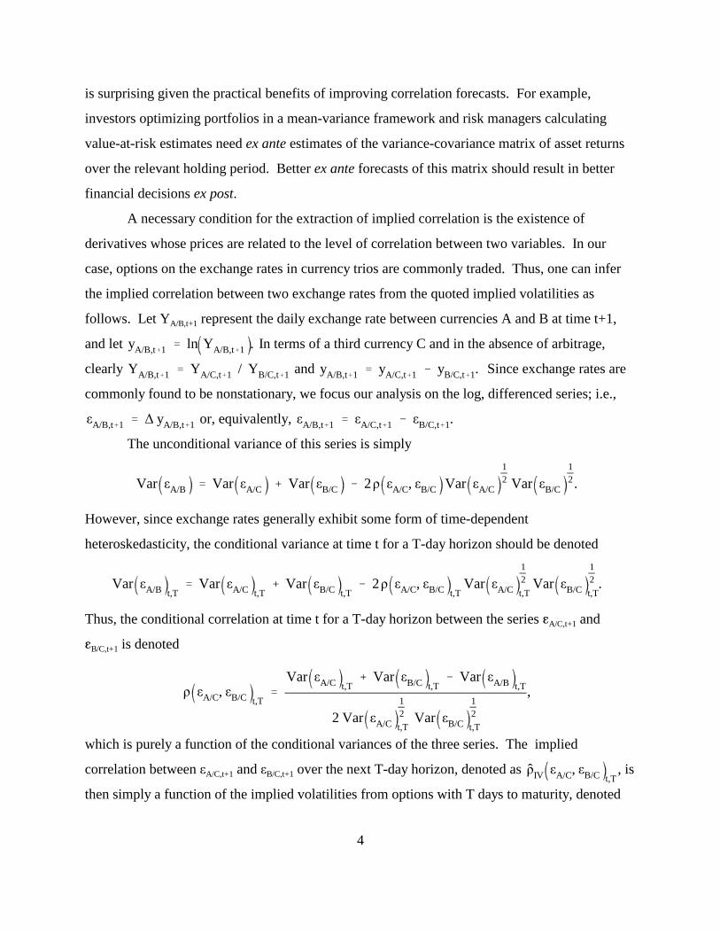
The unconditional variance of this series is simply

However, since exchange rates generally exhibit some form of time-dependent

heteroskedasticity, the conditional variance at time t for a T-day horizon should be denoted

Thus, the conditional correlation at time t for a T-day horizon between the seriesA/C,t+1 and

B/C,t+1 is denoted

which is purely a function of the conditional variances of the three series. The implied

correlation betweenεA/C,t+1 andεB/C,t+1 over the next T-day horizon, denoted as , isρIV εA/C, εB/C t,T

then simply a function of the implied volatilities from options with T days to maturity, denoted

3 Note that option prices are stated in units of implied volatilities, which are really standard deviations.The common practice for converting these implied standard deviations into variances is simply to square them.

4 Note that the three implied correlations in a currency trio are not independent of each other. See Singer,Terhaar and Zerolis (1998) for a discussion of the geometric relationship between the volatilities and thecorrelations in a currency trio.

5 Gibson and Boyer (1997) examine the use of correlations in an option-trading exercise in order tocompare alternative correlation forecasts. However, they do not use implied correlations in their study.

5

ρIV εA/C, εB/C t,T

ˆVarIV εA/C t,T ˆVarIV εB/C t,T

ˆVarIV εA/B t,T

2 ˆVarIV εA/C

12

t,TˆVarIV εB/C

12

t,T

.

;3 i.e.,ˆVarIV x t,T

Note that any of the three currencies could serve as a base currency and that andρIV εA/B, εC/B t,T

would be formed analogously.4ρIV εB/A, εC/A t,T

b. Literature review

To date, implied correlation between FX rates has been the subject of studies by Bodurtha

and Shen (1995); Siegel (1997); and Campa and Chang (1997).5 Bodurtha and Shen (1995) use

options price data from the Philadelphia Stock Exchange to examine ,ρIV εDEM/USD, εJPY/USD t,T

the implied correlation betweenεDEM/USD andεJPY/USD. They evaluate the forecasting ability of

implied correlation by regressing the observed, one-month correlations on one-month, implied

correlations and several time-series correlation forecasts. They find that both historical and

implied correlations provide useful information in forecasting realized correlation.

Siegel (1997) analyzes the forecasting performance of implied correlation in the context

of a specific application; i.e., whether implied correlations improve the performance of cross-

currency hedges. Again, using options data from the Philadelphia Stock Exchange on two

currency trios (the USD/DEM/JPY trio and the trio consisting of USD, DEM and the British

pound), options-based hedge ratios for several currency positions were constructed. The

volatilities of these hedged positions were then compared with the volatilities of hedged positions

based on simple, time-series correlation forecasts. Siegel finds that the hedges based on implied

6 As shown by Cooper and Weston (1996), FX options are among the fastest-growing groups of OTCinstruments and have become the subject of intense competition. As a consequence, their terms and conditionshave been standardized, and the differences in competing quote prices have become relatively small (less than onepercent of the average price).

6

correlations perform significantly better in some cases and never significantly worse than the

time-series hedges. Furthermore, regression results indicate that the hedge ratios based on

historical correlations provide no additional information beyond that already reflected in the

hedge ratios based on implied correlations.

Unlike these two papers, Campa and Chang (1997) use data from the over-the-counter

(OTC) market for FX options, which has three important advantages. First, since the OTC

market for FX options is larger and more liquid than the market for these exchange-traded

options, the OTC prices should be more informative than those from the Philadelphia Stock

Exchange.6 Second, in contrast to exchange-traded options that have specific expiration dates,

OTC options are issued daily with fixed times to maturity, which eliminates the need to adjust

the implied volatilities for the effects of the options’ time decay. Third, OTC options are

generally created with at-the-money, strike prices. Since the sensitivity of options with regard to

the underlying’s volatility (the so-called “vega”) is typically highest for at-the-money options,

OTC options data ensure that the most information about the expected volatility is captured in

the quoted prices. Beckers (1981) provides evidence supporting this view, finding that implied

volatilities from at-the-money options do as well in predicting future volatilities as weighted

averages of implied volatilities from different options. The loss of information incurred by using

only at-the-money options, as done here, should therefore be modest.

Campa and Chang (1997) also analyze the forecasting ability of ˆρIV εDEM/USD, εJPY/USD t,T.

Their study is based on six and a half years of daily data on the implied volatilities of OTC

options with constant times-to-maturity of one month and three months. As alternative forecasts

to implied correlation, they consider simple, time-series forecasts as well as correlation forecasts

generated by a rolling, bivariate GARCH(1,1) model. Applying a richer econometric

methodology than the other two papers, they find that implied correlation outperforms the other

forecasts. In particular, they find that none of the time-series forecasts are consistently capable of

providing additional information relative to the implied correlation forecasts.

7

In summary, these studies provide some evidence on the forecasting ability of implied

correlations. Given the potential benefits, we further analyze this forecasting ability by

examining all three implied correlations extractable from the USD/DEM/JPY and

USD/DEM/CHF trios, which have markedly different characteristics.

III. Option Prices and Historical Data

a. Implied Correlations from Options Prices

The options prices used in this paper were provided by a prominent bank dealing in the

OTC market for FX options. The data consist of daily, one-month and three-month implied

volatilities for the three currency pairs in a currency trio. For the USD/DEM/JPY trio, data from

October 2, 1990 through April 2, 1997 (1679 observations) are available, and for the

USD/DEM/CHF trio, data from September 13, 1993 through April 2, 1997 (910 observations)

are available. We thus compare the forecast performance of twelve correlations (two currency

trios with three correlations each for two forecast horizons).

The implied volatilities are for at-the-money forward straddles, a combination of a

European call option and a European put option with the strike prices set at the forward rate.

Although the implied volatilities are derived from the Garman-Kohlhagen pricing model, they

are probably subject to model misspecification problems since this model assumes constant

volatility. However, as per Hull and White (1987), the pricing impact of time-varying volatility

should be small for options with less than one year to maturity. We thus do not correct the

implied volatilities for the presence of this misspecification error.

Figure 1 depicts the implied correlations for the two currency trios, and Table 1 presents

the corresponding summary statistics. Note that the two currency trios have markedly different

correlation structures. The implied correlations for the USD/DEM/JPY (or yen) trio differ much

less in their means and standard deviations than those for the USD/DEM/CHF (or franc) trio, as

clearly seen in the figure. Specifically, has a much higher mean andρIV εDEM/USD, εCHF/USD t,T

lower standard deviation than the other five correlations analyzed, which is indicative of the

7 Note that Switzerland is not a member of the European Monetary System and that the Swiss franc is notlinked to the German mark. Thus, there are no explicit, legally binding restrictions on these exchange rates.

8

ρ εA/C, εB/C t,T

T

i1εA/C,ti µA/C εB/C,ti µB/C

ΣT

i1εA/C,ti µA/C

2 ΣT

i1εB/C,ti µB/C

2

,

close economic relationship between Germany and Switzerland.7

b. Realized Correlation

Correlation, as with all higher moments of time-series data, is not directly observable.

Thus, the realized correlation over a horizon of T days must be proxied for by a consistent,

empirical estimate. In this case, the realized correlation between the log, differenced exchange

ratesA/C,t+1 andB/C,t+1 at time t over a T-day horizon is calculated as

where and are the corresponding sample means over the T-day period. The spotµA/C µB/C

exchange rate data used to calculate the realized correlations (and the alternative correlation

forecasts) is from the Swiss National Bank and consists of daily spot exchange rates from

January 3, 1980 through July 2, 1997, which is the in-sample estimation period.

In this paper, we focus on the one-month and three-month horizons matching the options

data. In the OTC market for FX options, the maturity of a contract is defined by calendar time;

i.e., an n-month option started on the date mm/dd/yy expires on the date mm+n/dd/yy if this day

is a weekday or the next workday if it falls on a weekend. Hence, the option’s time to maturity

measured in days is variable, depending on the calendar month. For our data set, the effective

number of trading days for the one-month horizon ranges from 18 to 23 with a mean of 21.9 and

a standard deviation of 1.0. For the three-month horizon, the effective number of trading days

ranges from 59 to 66 with a mean of 64.7 and a standard deviation of 1.4. In order to reduce

measurement error in the realized and forecasted correlations, we allow the maturity of the

option, as measured in days, to vary in our calculations.

9

ρH(n) εA/C, εB/C t

n

i1εA/C,ti1 µA/C εB/C,ti1 µB/C

Σn

i1εA/C,ti1 µA/C

2 Σn

i1εB/C,ti1 µB/C

2

,

ρE(λ,k) εA/C, εB/C t

k

i0λi εA/C,ti µA/C εB/C,ti µB/C

Σk

i0λi εA/C,ti µA/C

2 Σk

i0λi εB/C,ti µB/C

2

,

c. Simple Correlation Forecasts

The first category of time-series, correlation forecasts examined are based on rolling

averages of the products of past exchange rate changes. We consider two approaches that differ

only in the weights applied in the averages. Specifically, historical correlation equally weights

all observations, and exponentially-weighted moving average (EWMA) correlation is based on

weights that decline exponentially; i.e., for integer i > 0, whereλ is a calibratedwi λi

parameter. Note that both methods assume that the correlation forecasts are independent of the

forecast horizon; i.e., where the horizons T1 and T2 are notρm εA/C, εB/C t,T1

ρm εA/C, εB/C t,T2

,

the same. Hence, these simple forecasts imply a flat term-structure of correlation.

Historical Correlation

The historical correlation forecast at time t for any forecast horizon is defined as the

realized correlation over a fixed number of trading days prior to time t; i.e.,

where n denotes the number of trading days in the “observation period”. Note that all n

observations within the observation period are given equal weight, and all observations older

than n days are given zero weight. Since there is no obvious way to select n, we examine the

performance of historical correlation forecasts based on 20, 60 and 120 days of data or roughly

one, three and six months, respectively.

Exponentially-Weighted Moving Average Correlation

The EWMA correlation forecast at time t for any forecast horizon is defined as

8 For an overview of multivariate GARCH models, see Bollerslev, Engle, and Nelson (1994).

10

Ht1

h11,t1 h12, t1

h12, t1 h22, t1

,

whereλ (0,1) is the decay factor and k is the number of historical observations used in the

calculation. The EWMA approach, well known due to its use by J.P. Morgan’s RiskMetrics™

system for forecasting variances and covariances, offers two advantages over the previous

approach. First, by giving recent data more weight, the forecasts react faster to short-term

movements in exchange rates. Second, by exponentially smoothing out the effect of a given rate

change, EWMA forecasts do not exhibit the abrupt changes common to historical forecasts once

such a change falls out of the observation period.

The decay factorλ determines the relative weights applied to the observations; lower

values ofλ imply faster rates of decay in the influence of a given observation. Following

Hendricks (1996), we consider three different decay factors:λ = 0.94, 0.97, and 0.99. We

arbitrarily set k = 1250 such that the difference is negligible for all three values.Σ

i0λi

Σk

i0λi

Since k is constant, the three EWMA correlation forecasts are simply denoted E(0.94), E(0.97),

and E(0.99), respectively.

d. Correlation Forecasts Based on a Bivariate GARCH(1,1) Model

As developed by Engle (1982) and Bollerslev (1986), the univariate GARCH model has

become an established method for characterizing the variance dynamics found in financial time

series. In the bivariate GARCH model, the covariance also evolves over time and is specified in

a manner similar to that in the univariate case.8 The basic structure of the model for

is that the components of the conditional variance-εt1 εA/C,t1, εB/C,t1 ε1,t1, ε2,t1

covariance matrix Ht+1 vary through time as functions of the products of the observed innovations

and past values of Ht+1. Specifically,

where h11,t+1 and h22,t+1 are the variances of the two series and h12,t+1 is their covariance.

11

vech Ht1 W A vech εt εt B vech Ht ,

h11, t1

h12, t1

h22, t1

ω11

ω12

ω22

α11 α12 α13

α21 α22 α23

α31 α32 α33

ε21,t

ε1,tε2,t

ε22,t

β11 β12 β13

β21 β22 β23

β31 β32 β33

h1,t

h12, t

h2, t

.

h11, t1

h12, t1

h22, t1

ω11

ω12

ω22

α11 0 0

0 α12 0

0 0 α22

ε21,t

ε1,tε2,t

ε22,t

β11 0 0

0 β12 0

0 0 β22

h11,t

h12,t

h22,t

,

A common specification of a bivariate Gaussian, GARCH process is that

whereεt1 Ωt N 0, Ht1 ,

where vech is the vector-half operator that converts (N x N) matrices into (N(N+1)/2 x 1)()

vectors of their lower triangular elements, W is a (3 x 1) parameter vector, and A and B are (3x3)

parameter matrices. Alternatively, the model takes the matrix form,

Given the model’s 21 parameters, numerical maximization of the likelihood function is generally

too cumbersome. To enforce parametric parsimony, we follow Bollerslev, Engle and

Wooldridge (1988), who specify the A and B matrices to be diagonal and reduce the number of

parameters to just 9; i.e.,

which implies that for i,j = 1,2.hij, t1 ωij αij εi,t εj,t βij hij, t

Table 2, Panels 1 and 2 present the estimated parameters for the bivariate GARCH(1,1)

model over the entire in-sample period of January 3, 1980 through October 2, 1990. Since we

forecast all the correlations in the two currency trios, we estimate this model for the six exchange

rate pairs. Given that some studies, such as Hsieh (1989) and Bollerslevet. al.(1994), have

found significant first-order autocorrelations in the logged, first differences of FX rates, we

estimated the model’s conditional mean with and without an MA(1) term. That is, the

conditional mean is specified as where100∆yt1 µ θεt εt1, yt1 yA/C,t1; yB/C,t1

andθ is a diagonal matrix, and as where the diagonal elements ofθ are set100∆yt1 µ εt1,

to zero. Using the likelihood-ratio test, we find that the simpler specification cannot be rejected

12

Et hij, tk

ωij αij εij, t βij hij, t if k 1

ωij k1

s0αij βij

s αij βij

k1Et hij, t1 if k>1.

ρG εA/C, εB/C t,T

Et h12, t,T

Et h11, t,T Et h22, t,T

.

in favor of the MA(1) specification; see the LRMA statistics in Table 2. Based on this result, we

use the simple conditional mean specification to generate the GARCH-based correlation

forecasts. Note that these estimates, as often found in the literature, suggest considerable

persistence since is above 0.9 in all cases.αij βij

GARCH parameters derived from models estimated over the entire data sample obviously

reflect all of that information. In order to avoid giving the GARCH-based correlation forecasts

the advantage ofex postparameterization, we more closely approximate actual forecasting with

“rolling GARCH” estimations using the 1000 observations prior to the date on which the forecast

is made. Table 2, Panel C contains the parameter estimates forεDEM/USD andεJPY/USDfor the 1000

datapoints before the first out-of-sample, forecasting date (October 2, 1990). The last three

columns of the table report the mean, minimum and maximum parameter values, which indicate

variation in the parameter estimates over time. Although the estimated parameters vary over

time, they generally remain in small ranges that do not change the overall inference. Similar

results are obtained for the other exchange rate pairs.

The correlation forecasts generated from a GARCH model are different from the forecasts

generated by the simpler models in an important way. The previous models assume that the

daily, FX variances and covariances are constant, and thus, a forecast of the T-day correlation is

exactly equal to the past observed correlation. However, for the GARCH model, forecasts of Ht+1

change daily; the k-step-ahead forecast of hij at time t is

Since the daily innovations are not serially correlated, the forecast at time t of an element of Ht+1

over the subsequent T-day period is equal to The correspondingEt hij, t,T T

s1Et hij, ts .

correlation forecast is thenρG εA/C, εB/C t,T

Since we want to analyze the performance of the various correlation forecasts for two forecast

13

horizons, the rolling GARCH parameter estimates for the six exchange rate pairs are used to

generate the twelve GARCH-based correlation forecasts of interest. As with the realized

correlation, we take account of the effective number of trading days of the option contract used to

extract the corresponding implied correlation.

IV. Evaluating the Predictive Accuracy of the Correlation Forecasts

Figure 2 illustrates some typical properties of the various forecasts. The graphs show the

realized correlation and the corresponding forecasts. Clearly, realizedρ εDEM/USD, εJPY/USD t,T

correlation is much more variable than both the implied and GARCH-based forecasts. The

simple, time-series forecasts show the typical properties documented by Hendricks (1996). For

historical correlation, the longer the observation period, the less variable the forecast. For the

EWMA forecasts, the higher the decay factor, the longer the effective observation period and,

consequently, the less variable the forecast.

In this section, we evaluate the predictive accuracy of the competing forecasts presented

above using three types of forecast evaluation criteria. The first two criteria examine the

properties of the individual forecasts themselves, and the third criteria examines their relative

performance. Below, we describe the three criteria and report our empirical results.

a. Three Types of Forecast Evaluation Criteria

Analysis of Forecast Errors

The first type of evaluation criteria is based on the analysis of the forecast errors, defined

as where is the forecast of the correlation atem,t ρm εA/C, εB/C t,T ρ εA/C, εB/C t,T

, ρm()t,T

time t generated by model m. To evaluate the performance of the various forecasts, we calculate

the mean forecast errors (MFEs) and the root-mean-squared forecast errors (RMSFEs). A

standard property of optimal forecasts is that they are unbiased, which implies that the forecast

errors have zero means. To test for this property, we regress em,t on a constant using the Newey

and West (1987) standard errors to account for unknown heteroskedasticity and autocorrelation.

If that coefficient is significantly different from zero, then the forecast is said to be biased.

14

ρ ()t,T a b ρm()t,T νt.

We then compare the relative RMSFEs using the test proposed by Diebold and Mariano

(1995). Taking root-mean-squared error as the relevant loss function, for a particular correlation,

we generate the time series of the differences between the loss function values of each forecast

and the best forecast in RMSFE terms. If two forecasts are equally accurate, then the mean of

this difference should be zero. If we reject this null hypothesis, then the forecast with the lower

RMSFE is truly the more accurate forecast. The asymptotic Diebold-Mariano statistic tests the

hypothesis with what is essentially a t-statistic that this mean is zero.

Partial Optimality Regressions

The second type of evaluation criteria assesses the partial optimality of the various

forecasts. Partial optimality refers to whether the forecast errors are unforecastable with respect

to some subset of available information; see Brown and Maital (1981) as well as the discussion

in Diebold and Lopez (1996). In our analysis, if a forecast is partially optimal, then the forecast

error should be orthogonal to the forecast itself. Following Mincer and Zarnowitz (1969), we test

for the partial optimality of the correlation forecasts by running regressions of the following type

Partial optimality of a forecast corresponds to parameter estimates of (a,b) that are insignificantly

different from zero and one, respectively. Deviation from those parameter values is evidence that

the forecast errors are not orthogonal to the forecasts themselves; i.e., if the forecast errors are

correlated with the forecasts, the forecasts do not make optimal use of the data used to form

them.

Encompassing Regressions

The third type of evaluation criteria uses multiple regression analysis to assess the

information content of different forecasts. The so-called encompassing regressions enable us to

determine whether a certain forecast incorporates (or encompasses) all the relevant information

in competing forecasts; see Chong and Hendry (1986) for further discussion. To illustrate the

idea, consider the case of two correlation forecasts, and . If the regressionρ1()t,T ρ2()t,T

9 Note that the RMSFEs tend to be lower for the three-month correlations than for the one-monthcorrelations, suggesting that correlation forecasts tend to be more accurate for longer forecast horizons, possiblyreflecting reversion to the unconditional covariance over long time periods.

15

ρ ()t,T γ0 γ1 ρ1()t,T γ2 ρ2()t,T νt

results in parameter estimates (γ0, γ1, γ2) that are not significantly different from (0, 1, 0), then

forecast 1 is said to encompass forecast 2; i.e., the information set used to form forecast 1

encompasses that used to form forecast 2. Similarly, if the parameter estimates are not

significantly different from (0, 0, 1), forecast 2 encompasses forecast 1. For any other values,

neither model encompasses the other, and both forecasts contain useful information.

In order to test for the information contribution of the various forecasts, we estimate

encompassing regressions for every correlation analyzed. Since the simple forecasts tend to be

correlated among themselves, we do not include them all as right-hand variables. Instead, we

include the two “sophisticated” forecasts of implied and GARCH-based correlation along with

one historical and one EWMA forecast. We choose one each from among the historical and

EWMA correlations according to the maximal R2's from the partial optimality regressions.

b. Empirical Results for the Various Correlation Forecasts

Analysis of Forecast Errors

Table 3 reports the mean forecast errors (MFEs) and root-mean-squared forecast errors

(RMSFEs) for both the one-month and three-month maturities of each currency trio.9 For both

trios, the MFE results indicate that the sophisticated forecasts generally have larger forecast

biases than the simple forecasts, and these biases are significant in 19 of 24 cases. The small

MFEs of the simple correlation forecasts are not surprising, given that they approximate the

unconditional correlation of the series using a subsample of the available data. However, the bias

in the sophisticated forecasts is harder to explain, although Jorion (1995) found significant biases

for implied volatility forecasts from FX options.

Yet, the reported RMSFE and Diebold-Mariano (D&M) test results indicate that the

10 Note the low variability of is reflected in the relatively small size of theρ εDEM/USD, εCHF/USD t,TRMSFEs of its forecasts, which are about four to ten times smaller than those of the other correlations analyzed.Note further that there is a high degree of correspondence in the accuracy of the forecasts

and , due to the fact that the correlations in a currency trio areρ εUSD/DEM, εCHF/DEM t,Tρ εUSD/CHF, εDEM/CHF t,T

related. Given that is relatively constant, the mutual dependency of the three correlationsρ εDEM/USD, εCHF/USD t,Timplies that the forecast errors for the other two correlations in this trio will be related in absolute size.

16

unbiased nature of the simple forecasts does not imply that they necessarily have a closer

relationship to the realized correlations. For the yen trio, the implied and GARCH-based

forecasts generate the lowest RMSFEs in all six cases. (Note that the minimum RMSFE in each

column is marked in bold.) Furthermore, the D&M results indicate that these sophisticated

forecasts are never significantly different than the forecast with the lowest RMSFE. Thus, the

sophisticated forecasts perform quite well under the RMSFE criteria for this currency trio.

However, their performance for the franc trio is not as good. The implied and GARCH-

based forecasts minimize RMSFE only once each among the six cases. Whereas implied

correlation performs relatively well for , its performance with respect toρ εDEM/USD, εCHF/USD t,T

the other two correlations is poor.10 Not only do the option-based forecasts for these two

correlations exhibit RMSFEs that are significantly larger than the RMSFEs of the best respective

forecasts, they also have MFEs (or bias) of an order of magnitude (going up to almost 0.3 in

absolute size) that questions their usefulness in predicting these correlations. Note that the

GARCH-based forecasts are never significantly different from the minimizing forecasts.

A clear conclusion that arises from these results is that the implied correlations are not

uniformly the best forecasts of realized correlation. Although they perform well for the yen trio,

their performance for the franc trio indicates that implied correlations may not always be the best

forecast available and may not be worth calculating.

Partial Optimality Regressions

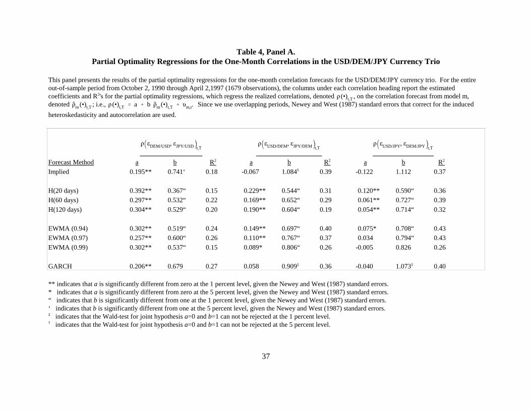
The results for the partial optimality regressions are reported in Table 4. For both trios,

the simple forecasting methods consistently violate both conditions that a partially optimal

forecast must fulfill; i.e., (a,b) = (0,1). Only one of the 72 sets of such forecasts examined (i.e.,

one-month ) is found to pass the individual tests for partialρE(0.90) εUSD/JPY, εDEM/JPY t,T

optimality, but not the joint test.

11 While a variety of such regression results are reported in the literature, the R2's for the regression ofrealized volatility on a constant and implied volatility are generally lower. Jorion (1995) reports R2's in the range of0.02 to 0.05. Galati and Tsatsaronis (1995) report an R2 of 0.30 in the case of the USD/ British pound, and Guo(1996) reports a R2 of 0.10 for the USD/JPY volatility.

17

With respect to the sophisticated forecasts, there are once again important differences in

performance between the two currency trios. For the yen trio, these forecasts generally perform

better. In eight out of twelve cases, the null hypothesis of a=0 is not rejected, and only in three

cases is the null hypothesis of b=1 rejected. In fact, two implied correlation forecasts and three

GARCH-based forecasts pass the joint test of partial optimality. Yet, this good performance

does not necessarily imply better goodness-of-fit measures; i.e., these forecasts provide the

highest adjusted R2's in just three of the five cases. Note that R2's for the correlation forecasts are

substantially higher than reported results for the implied volatilities of FX rates.11 This result is

consistent with the view that, at least for some financial variables, correlations tend to be more

stable and more predictability than volatilities.

However, for the franc trio, none of the forecasts are consistently partially optimal. Of

the twelve cases examined, only three-month does not reject the jointρG εDEM/USD, εCHF/USD t,T

null hypothesis of partial optimality. The regression results also confirm that the forecasts’

performance is not uniform over the three correlations in the trio. Specifically, implied

correlation performs much better with respect to with R2's of 0.37 andρ εDEM/USD, εCHF/USD t,T

0.27 for the one- and three-month horizons, respectively. The R2’s for the other two correlations

are below 0.10. These results indicate that the implied correlations for this currency trio do not

efficiently incorporate the information upon which they are based. There are a number of

possible reasons for this result, such as low trading volume, improper use of the option pricing

model or misspecification of the option pricing model.

Encompassing Regressions

Table 5 reports the results for the encompassing regressions in which the realized

correlations are regressed on a constant and a set of forecasts. For each case of the twelve cases,

the set includes implied correlations, the GARCH-based correlation forecasts, and the historical

and EWMA correlation forecasts with the highest R2 in the partial optimality regressions. In

18

general, the encompassing regressions for both trios provide mixed results with regard to the

usefulness of implied correlations for forecasting realized correlations. Once again, implied

correlations are found to be useful in some, but not all, cases.

Specifically, for the yen trio, the three main results can be summarized as follows. First,

implied correlations do seem to contain information not present in the time-series forecasts in

certain cases. The coefficients on implied correlation are significantly positive in three of the six

cases. The second result is that implied correlations do not fully incorporate all the information

extractable from time-series data. The Wald test results, listed at the bottom of the table, never

reject the null hypothesis that the regression coefficients on all the time-series forecasts are zero,

suggesting that they are not encompassed by implied correlations and do provide additional

information useful in predicting realized correlation.

These findings are inconsistent with those of Campa and Chang (1997), who find that

time-series forecasts of do not contribute incremental information toρ εDEM/USD, εYEN/USD t,T

implied correlation forecasts. We currently attribute this difference in conclusions to the time

periods of the two studies. Campa and Chang’s study is based on data from January 3, 1989

through May 23, 1995, which overlaps with roughly the beginning 70 percent of our data from

October 2, 1990 through April 2, 1997. The different sample periods may give rise to different

results if there is time-variation in the forecasting ability of implied correlations. In fact, Table 6

provides some evidence that this may be the case. The table reports the results of encompassing

regressions for one-month based on eight, non-overlapping subsamplesρ εDEM/USD, εYEN/USD t,T

of 200 observations each. The table shows that the coefficient on implied correlation was

generally significant in the first half of the sample from October 1990 to October 1993.

However, for the second half of our data sample (November 1993 to April 1997), the coefficient

is generally insignificant, suggesting that the inclusion of implied correlations does not improve

the performance of the time-series forecasts. The fact that implied correlation performed

differently in these non-overlapping periods may explain the differences between Campa and

Chang’s and our results, but further analysis is necessary.

The third result from the encompassing regressions for the yen trio is that the GARCH-

based correlation forecasts seem to best incorporate the information in the historical, time-series

19

data. In three of six cases, the regression coefficient on the GARCH-based correlation forecast is

significant. The other forecasts based on historical data do not consistently provide incremental

information useful in forecasting, although the Wald test never rejects the null hypothesis that the

coefficients on all the time-series forecasts are zero.

With respect to the franc trio, Table 5, Panels C and D report the results of the

encompassing regressions. Once again, there is no forecast that consistently provides useful

information not contained in the other forecasts. Implied correlation incrementally improves the

performance of the other forecasts for , which has the least variability ofρ εDEM/USD, εCHF/USD t,T

all the realized correlations examined. For the two other correlations, the coefficients on implied

correlation are never significantly positive. (In fact, far from demonstrating implied correlation’s

predictive ability, they are even negative in two cases.) While the GARCH-based forecasts do

not add information for , they tend to provide incremental information forρ εDEM/USD, εCHF/USD t,T

the two other correlations. As for the simple forecasts, whereas the coefficients on the historical

correlations are never significant, some of the EWMA forecasts do provide additional

information useful in forecasting the realized correlation. However, there is no EWMA-based

forecasts that adds information across all the correlations in the trio. In short, the encompassing

regressions for the franc trio are generally less clear than those for the yen trio.

V. Conclusion

Several papers, such as Jorion (1995), indicate that implied volatilities from foreign

exchange options are useful in forecasting subsequently realized volatility. This paper addresses

the question of whether implied correlations are useful in forecasting subsequently realized

correlation. Using daily, OTC data on exchange rate options in two currency trios, we examine

all six of the implied correlations extractable. We compare the forecasting performance of these

implied correlations against a number of alternative, time-series forecasts, such as simple

historical correlations and correlation forecasts generated by a rolling, bivariate GARCH(1,1)

model. Our main finding is that the performance of the implied correlations varies significantly

across the currency trios and even across time periods.

For the yen trio, we find that although implied and GARCH-based correlation forecasts

20

are biased, they generate lower root-mean-squared forecast errors than simple, time-series

forecasts. Moreover, these forecasts are generally shown to be partially optimal with respect to

the information sets used to create them. Encompassing regressions reveal that although each

individual forecast has some predictive power, only implied and GARCH-based correlations

provide useful information not present in the other forecasts. Thus, even though implied

correlations do not fully incorporate all the information in the price history, they do contain

information not found in it. This result indicates that implied correlations are worth calculating,

but we also find that their performance, as well as that of the other forecasts, varies over time.

The results for the franc trio reveal that the value of implied correlation as a predictor of

future realized correlation is not uniform across currency trios. We find that both in terms of

accuracy and information content, implied correlation is useful in forecasting

in this trio. However, the economic benefits of employing the option-ρ εDEM/USD, εCHF/USD t,T

based forecast in this case is small due to the low variability of this correlation. For the two other

correlations in the trio, implied correlation is far from being superior to the time-series forecasts,

although these forecasts also do not consistently provide good forecasts for the correlations in

this trio. Only GARCH-based correlation appears to have at least some forecasting ability,

providing useful forecasts for two of the three correlations.

The absence of significant forecast performance from the implied correlations in the franc

trio as well as its inconsistent performance for the yen trio seem to challenge the value of implied

correlations as predictors of realized correlation. From our results, we conclude that its

predictive ability can only be determined empirically. These results raise the important question

of why such option-based forecasts, which ostensibly include the price history as well as the

market’s expectations over the option’s maturity, do not consistently outperform the time-series

forecasts. There are two possible reasons for this poor performance. First, it could be that the

Garman-Kohlhagen (1983) option pricing model commonly used to extract FX implied

volatilities is misspecified. Second, it could be that the market for some of the options used to

extract the implied correlations is not efficient. Although this seems unlikely for the yen trio, it

is possible that the trading volume for options in the franc trio is not large enough to assure

accurate market prices. Further research is needed to answer these questions.

21

References

Amin, K.I. and Ng, V.K., 1997. “Inferring Future Volatility from the Information in ImpliedVolatility in Eurodollar Options: A New Approach,”Review of Financial Studies, 10,333–367.

Beckers, S., 1981. “Standard Deviations Implied in Option Prices as Predictors of Future StockPrice Variability,”Journal of Banking and Finance, 5, 363–381.

Bodurtha, J.N. and Shen, Q., 1995. “Historical and Implied Measures of ´Value at Risk´: TheDM and Yen Case,” Manuscript, Georgetown University.

Bollerslev, Tim. 1986. “Generalized Autoregressive Conditional Heteroskedasticity”.Journal ofEconometrics. 31, 307–327.

Bollerslev, T. and Engle, R.F., 1993. “Common Persistence in Conditional Variances,”Econometrica, 61, 167-186.

Bollerslev, T., Engle, R.F. and Wooldridge, J.M., 1988. "A Capital Asset Pricing Model withTime-Varying Covariances,"Journal of Political Economy, 96, 116-131.

Bollerslev, T., Engle, R.F. and Nelson, D.B., 1994. "ARCH Models," in Engle, R.F. andMcFadden, D., eds.The Handbook of Econometrics, Volume 4, 2959-3038. Amsterdam:North-Holland.

Brown, B.W. and Maital, S., 1981. “What Do Economists Know? An Empirical Study ofExperts’ Expectations,”Econometrica, 49, 491–504.

Campa, J.M. and Chang, P.H.K., 1997. “The Forecasting Ability of Correlations Implied inForeign Exchange Options,” NBER Working Paper #5974.

Chong, Y.Y. and Hendry, D.H., 1990. “Econometric Evaluation of Linear Macro-EconometricModels,”Review of Economic Studies, 53, 671–690.

Cooper, S. and Weston, S., 1996. “Bank Checks,”Risk, 9 (2), 23–27.

Diebold, F.X. and Mariano, R.S., 1995. “Comparing Predictive Accuracy,”Journal of Businessand Economic Statistics,13, 253-263.

Diebold, F.X. and Lopez, J.A., 1996. “Forecast Evaluation and Combination,”The Handbook ofStatistics, Volume 14: Statistical Methods in Finance, G.S. Maddala and C.R. Rao (eds.).Amsterdam: North-Holland, 241-268.

22

Engle, R.F., 1982. "Autoregressive Conditional Heteroskedasticity with Estimates of theVariance of U.K. Inflation,"Econometrica, 50, 987-1008.

Galati, G. and Tsatsaronis, C., 1995. “The Information Content of Implied Volatility fromCurrency Options,” Manuscript, Bank for International Settlements.

Garman, M. B. and Kohlhagen, S.W., 1983. “Foreign Currency Option Values,”Journal ofInternational Money and Finance, 2, 231–237.

Gibson, M.S. and Boyer, B.H., 1997. “Evaluating Forecasts of Correlation Using OptionPricing,” International Finance Discussion Papers #600, Board of Governors of theFederal Reserve System.

Guo, D., 1996. “The Predictive Power of Implied Stochastic Variance from Currency Options,”Journal of Futures Markets, 16, 915-942.

Hendricks, D., 1996. “Evaluation of Value-at-Risk Models Using Historical Data,”FederalReserve Bank of New York Economic Policy Review, 2, 39–69.

Hsieh, D.A., 1988. "The Statistical Properties of Daily Foreign Exchange Rates: 1974-1983,"Journal of International Economics, 24, 129-145.

Hull, J.C. and White, A., 1987. “The Pricing of Options with Stochastic Volatility,”Journal ofFinance, 42, 281–300.

Jorion, P., 1995. “Predicting Volatility in the Foreign Exchange Market,”Journal of Finance,50, 507-528.

J.P. Morgan, 1996.RiskMetrics™ – Technical Document. Fourth edition, New York: J.P.Morgan.

Kroner, K.F., Kneafsey, K.P. and Claessens, S., 1995. “Forecasting Volatility in CommodityMarkets,”Journal of Forecasting, 14, 77–95.

Karolyi, G.A. and Stulz, R., 1996. “Why Do Markets Move Together? An Investigation of U.S.-Japan Stock Return Comovements,”Journal of Finance, 51, 951-986.

Longin, F. and Solnik, B., 1995. “Is the Correlation in International Equity Returns Constant:1960-1990?,”Journal of International Money and Finance, 14, 3-26.

Mahoney, J.M., 1995. “Correlation Products and Risk Management Issues,”Federal ReserveBank of New York Economic Policy Review, 1, 7–20.

23

Mayhew, S., 1995. “Implied Volatility,”Financial Analysts Journal, July-August, 8–20.

Mincer, J. and Zarnowitz, V., 1969. “The Evaluation of Economic Forecasts,” in Mincer, J.(ed.). Economic Forecasts and Expectations. National Bureau of Economic Research:New York.

Newey, W.K. and West, K.D., 1987. “A Simple Positive Semi-Definitive Heteroskedasticity andAutocorrelation Consistent Covariance Matrix,”Econometrica, 55, 703–708.

Siegel, A.F., 1997. “International Currency Relationship Information Revealed by Cross-OptionPrices,”Journal of Futures Markets, 17, 369-384.

Singer, B.D., Terhaar, K. and Zerolis, J., 1998. “Maintaining Consistent Global Asset Views(with a Little Help from Euclid),”Financial Analysts Journal, January/February, 63-71.

24

Table 1, Panel A.Descriptive Statistics for the Implied Correlations in the USD/DEM/JPY Currency-Trio

This panel presents the means, standard deviations, coefficients of skewness and kurtosis, and maximumand minimum values for implied correlations, as calculated from the implied volatilities of at-the-money, FX optionswith the forward rate set as the strike price. The notation refers to the implied correlation at time tρIV εA/C, εB/C t,Tderived from the implied volatilities on options with maturities of T months for the changes in the logged, exchangerates between currencies A and B with respect to currency C. The observation period is October 2, 1990 throughApril 2,1997, which generates 1679 observations.

Mean Std.Dev. Skewness Kurtosis Maximum Minimum

0.5691 0.1094 -0.3726 3.0431 0.8198 0.0471ρIV εDEM/USD,εJPY/USD t,1

0.5687 0.0858 -0.1289 2.4269 0.7737 0.3021ρIV εDEM/USD,εJPY/USD t,3

0.5243 0.1688 0.0036 2.4829 0.8952 -0.0480ρIV εUSD/DEM,εJPY/DEM t,1

0.5161 0.1513 -0.0521 2.3061 0.8209 0.0303ρIV εUSD/DEM,εJPY/DEM t,3

0.3755 0.1970 -0.6063 2.8926 0.7817 -0.4140ρIV εUSD/JPY,εDEM/JPY t,1

0.3930 0.1570 -0.6988 2.7740 0.6911 -0.1470ρIV εUSD/JPY,εDEM/JPY t,3

25

Table 1, Panel B.Descriptive Statistics for the Implied Correlations in the USD/DEM/CHF Currency-Trio

This panel presents the means, standard deviations, coefficients of skewness and kurtosis, and maximumand minimum values for implied correlations, as calculated from the implied volatilities of at-the-money, FX optionswith the forward rate set as the strike price. The notation refers to the implied correlation at time tρIV εA/C, εB/C t,Tderived from the implied volatilities on options with maturities of T months on the changes in logged, exchangerates between currencies A and B with respect to currency C. The observation period is September 13, 1993through April 2, 1997 (910 observations).

Mean Std.Dev. Skewness Kurtosis Maximum Minimum

0.9134 0.0347 -0.1551 2.1113 0.9815 0.8310ρIV εDEM/USD,εCHF/USD t,1

0.9169 0.0261 -0.0459 2.2126 0.9749 0.8506ρIV εDEM/USD,εCHF/USD t,3

-0.0216 0.1372 -0.3313 3.2780 0.4952 -0.4993ρIV εUSD/DEM,εCHF/DEM t,1

-0.0070 0.1175 -0.1516 2.6989 0.4166 -0.3968ρIV εUSD/DEM,εCHF/DEM t,3

0.4156 0.1133 0.0286 2.4365 0.6721 -0.1079ρIV εUSD/CHF,εDEM/CHF t,1

0.3979 0.1079 0.3202 2.1620 0.6301 -0.0033ρIV εUSD/CHF,εDEM/CHF t,3

26

ρ ρ

One-Month Three-Month

1/2/91 1/2/93 1/2/95 1/2/97-0.5

0

0.5

1

1/2/91 1/2/93 1/2/95 1/2/97-0.5

0

0.5

1

ρ ρ


1/2/91 1/2/93 1/2/95 1/2/97-0.5

0

0.5

1

1/2/91 1/2/93 1/2/95 1/2/97-0.5

0

0.5

1

ρ ρ


1/2/91 1/2/93 1/2/95 1/2/97-0.5

0

0.5

1

1/2/91 1/2/93 1/2/95 1/2/97-0.5

0

0.5

1

Figure 1, Panel A.One-Month and Three-Month Implied Correlations

in the USD/DEM/JPY Currency Trio

ρIV εDEM/USD,εJPY/USD t,T

ρIV εUSD/DEM,εJPY/DEM t,T

ρIV εUSD/JPY,εDEM/JPY t,T

27

ρ ρ


1/2/97 1/2/96 1/2/95 1/3/94-0.5

0

0.5

1

1/2/97 1/2/96 1/2/95 1/3/94-0.5

0

0.5

1

ρ ρ


1/2/97 1/2/96 1/2/95 1/3/94-0.5

0

0.5

1

1/2/97 1/2/96 1/2/95 1/3/94-0.5

0

0.5

1

ρ ρ


1/2/97 1/2/96 1/2/95 1/3/94-0.5

0

0.5

1

1/2/97 1/2/96 1/2/95 1/3/94-0.5

0

0.5

1

Figure 1, Panel B.One-Month and Three-Month Implied Correlations

in the USD/DEM/CHF Currency Trio

ρIV εDEM/USD,εCHF/USD t,T

ρIV εUSD/DEM,εCHF/DEM t,T

ρIV εUSD/CHF,εDEM/CHF t,T

28

100∆yt1 µ εt1

εt1 Ωt ~ N 0,Ht1

hij, t1 ωij αij εi, t εj, t βij hij, t,

Table 2, Panel A.

Bivariate GARCH(1,1) Parameter Estimatesfor the Exchange Rate Pairs in the USD/DEM/JPY Currency Trio

This panel reports the estimation results for the bivariate GARCH(1,1) model with a constant conditional mean forthe three exchange rate pairs in the USD/DEM/JPY currency-trio. The data observation period is from January 3,1980 through October 2, 1990 (2714 observations). Following Bollerslev, Engle and Wooldridge (1988), the modelis specified for the log exchange rates between currencies A and B with respect to currency C, denoted

, asyt1 yA/C,t1; yB/C,t1

where µ is a (2x1) constant conditional mean vector, Ht+1 is a (2x2) variance-covariance matrix and hij,t+1 is its i,jth

element where i,j = 1,2. LRMA is the likelihood ratio statistic testing the null-hypothesis of that the diagonal MA(1)matrixθ in the alternative conditional mean specification has parameters equal to zero.∆yt1 µ θεt εt1The statistic is distributedχ2(2).

DEMUSD & JPYUSD USDDEM & JPYDEM USDJPY & DEM JPY

Parameter Standard Parameter Standard Parameter StandardEstimate Error Estimate Error Estimate Error

-0.0065 0.0121 0.0083 0.0125 -0.0155 0.0115µ1

0.0118 0.0113 0.0208* 0.0082 -0.0186* 0.0075µ2

0.0185* 0.0027 0.0217* 0.0041 0.0276* 0.0033ω11

0.0149* 0.0019 0.0043* 0.0013 0.0048* 0.0007ω12

0.0244* 0.0027 0.0095* 0.0019 0.0074* 0.0013ω22

0.1353* 0.0100 0.1184* 0.0107 0.1276* 0.0092α11

0.1180* 0.0087 0.1202* 0.0100 0.1320* 0.0085α12

0.1196* 0.0098 0.1628* 0.0157 0.1512* 0.0117α22

0.8441* 0.0105 0.8470* 0.0125 0.8285* 0.0122β11

0.8551* 0.0094 0.8512* 0.0106 0.8421* 0.0099β12

0.8397* 0.0113 0.8159* 0.0157 0.8376* 0.0122β22

Log Likelihood -436.1 -436.5 -437.4

LRMA 0.018 0.326 0.576

* Indicates statistical significance at the 5 percent level.

29

100∆yt1 µ εt1

εt1 Ωt ~ N 0,Ht1


Table 2, Panel B.

Bivariate GARCH(1,1) Parameter Estimatesfor the Exchange Rate Pairs in the USD/DEM/CHF Currency Trio

This panel reports the estimation results for the bivariate GARCH(1,1) model with a constant conditional mean forthe three exchange rate pairs in the USD/DEM/JPY currency-trio. The data observation period is from January 3,1980 through October 2, 1990 (2714 observations). Following Bollerslev, Engle and Wooldridge (1988), the modelis specified for the log exchange rates between currencies A and B with respect to currency C, denoted

, asyt1 yA/C,t1; yB/C,t1

where µ is a (2x1) constant conditional mean vector, Ht+1 is a (2x2) variance-covariance matrix and hij,t+1 is its i,jth

element where i,j = 1,2. LRMA is the likelihood ratio statistic testing the null-hypothesis of that the diagonal MA(1)matrixθ in the alternative conditional mean specification has parameters equal to zero.∆yt1 µ θεt εt1The statistic is distributedχ2(2).

DEMUSD & CHFUSD USDDEM & CHFDEM USDCHF & DEM CHF

Parameter Standard Parameter Standard Parameter StandardEstimate Error Estimate Error Estimate Error

0.0003 0.0113 0.0034 0.0115 0.0049 0.0127µ1

-0.0025 0.0123 -0.0031 0.0045 0.0031 0.0046µ2

0.0163* 0.0027 0.0139* 0.0031 0.0171* 0.0040ω11

0.0153* 0.0025 0.0004* 0.0001 0.0030* 0.0007ω12

0.0172* 0.0029 0.0023* 0.0006 0.0026* 0.0006ω22

0.0874* 0.0066 0.1032* 0.0102 0.0965* 0.0098α11

0.0802* 0.0062 0.0584* 0.0092 0.0657* 0.0095α12

0.0765* 0.0062 0.0845* 0.0139 0.0957* 0.0127α22

0.8883* 0.0084 0.8799* 0.0106 0.8841* 0.0114β11

0.8967* 0.0079 0.9194* 0.0115 0.9050* 0.0138β12

0.9011* 0.0083 0.8923* 0.0188 0.8798* 0.0171β22

Log Likelihood -417.9 -418.8 -418.2

LRMA 0.442 0.206 0.460


30

100∆yt1 µ εt1

εt1 Ωt ~ N 0,Ht1


Table 2, Panel C.

Parameter Estimates for the Bivariate GARCH(1,1) Modelfor the Exchange Rate Pair yDEM/USD and yJPY/USD

This panel reports, in the first two columns, the estimation results for the bivariate GARCH(1,1) model with aconstant conditional mean for the exchange rate pair . The data observationyt1 yDEM/USD,t1; yJPY/USD,t1

period is the 1000 observations prior to October 2, 1990, the beginning of the relevant out-of-sample period.Following Bollerslev, Engle and Wooldridge (1988), the model is specified as

where Ht+1 is a (2x2) variance-covariance matrix and hij,t+1 is its i,jth element where i,j = 1,2. The last three columnssummarize the parameter values (minimum, maximum and mean) for the rolling GARCH estimations using 1,000observations and running from October 2, 1990 through April 2, 1997.

Model Rolling Modelfor October 2, 1990 from October 2, 1990 through April 2, 1997

Parameter Standard Minimum Maximum MeanEstimates Errors Value Value Value

0.0134 0.0204 -0.0140 0.0565 0.0206µ1

0.0171 0.0202 -0.0257 0.0462 0.0215µ2

0.0145* 0.0034 0.0044 0.0198 0.0127ω11

0.0140* 0.0025 0.0020 0.0149 0.0070ω12

0.0242* 0.0034 0.0073 0.0260 0.0152ω22

0.1205* 0.0152 0.0424 0.1208 0.0739α11

0.1204* 0.0124 0.0340 0.1219 0.0680α22

0.1298* 0.0143 0.0549 0.1326 0.0839α33

0.8637* 0.0161 0.8606 0.9371 0.9082β11

0.8578* 0.0129 0.8531 0.9561 0.9156β22

0.8358* 0.0151 0.8292 0.9300 0.8872β33


31

ρImplied

Realized

Jan/2/91 Jan/2/93 Jan/2/95 Jan/2/97-0.4

-0.2

0

0.2

0.4

0.6

0.8

1

ρBiv. GARCH(1,1)

Realized

Jan/2/91 Jan/2/93 Jan/2/95 Jan/2/97-0.4

-0.2

0

0.2

0.4

0.6

0.8

1

ρ

Historical (20-days)Realized

Jan/2/91 Jan/2/93 Jan/2/95 Jan/2/97-0.4

-0.2

0

0.2

0.4

0.6

0.8

1

Figure 2.One-Month Correlation for the Exchange Rate Pair yDEM/USD and yJPY/USD

from October 2, 1990 through April 2, 1997:Realized Correlation versus Various Forecasts

A. Realized and Implied Correlation

B. Realized and Biv. GARCH(1,1) based Correlation

C. Realized and 20 days Historical Correlation

32

ρ Historical (120-days)

Realized

Jan/2/91 Jan/2/93 Jan/2/95 Jan/2/97-0.4

-0.2

0

0.2

0.4

0.6

0.8

1

ρEWMA (Lambda=0.94)

Realized

Jan/2/91 Jan/2/93 Jan/2/95 Jan/2/97-0.4

-0.2

0

0.2

0.4

0.6

0.8

1

ρ EWMA (Lambda=0.99)

Realized

Jan/2/91 Jan/2/93 Jan/2/95 Jan/2/97-0.4

-0.2

0

0.2

0.4

0.6

0.8

1

Figure 2. - ContinuedOne-Month Correlation for the Exchange Rate Pair yDEM/USD and yJPY/USD

from October 2, 1990 through April 2, 1997:Realized Correlation versus Various Forecasts

D. Realized and 120 days Historical Correlation

E. Realized and EWMA (λ=0.94) Correlation

F. Realized and EWMA (λ=0.99) Correlation

33

MFE 1N

N

t1ρ (•)t,T ρm(•)t,T , and RMSFE 1

N N

t1ρ (•)t,T ρmt(•)t,T

2,

Table 3, Panel A.Analysis of Forecast Errors for the One-Month Correlation Forecasts in the USD/DEM/JPY Currency Trio

This panel presents the analysis of the forecast errors between the forecasted and realized correlations for all three currency pairs in the USD/DEM/JPY trio. Forthe entire out-of-sample period from October 2, 1990 to April 2, 1997 (1679 observations), the columns under each correlation heading report the meanforecasterrors (MFE), the root-mean-squared forecast errors (RMSFE), and the Diebold-Mariano test statistic (D&M Test) for the null hypothesis of no difference in theforecast accuracy under the root-mean-squared loss function. MFE and RMSFE are defined as

respectively, where denotes the realized correlation and denotes the correlation forecast according to model m. The statistical significance of theρ (•)t,T ρm(•)t,TMFEs is assessed by running regressions of the forecast errors on a constant; the standard errors of the estimated parameters are corrected for the inducedheteroskedasticity and autocorrelation using the Newey and West (1987) procedure. The minimum RMSFE value in each column is marked in bold.

ρ εDEM/USD, εJPY/USD t,Tρ εUSD/DEM, εJPY/DEM t,T

ρ εUSD/JPY, εDEM/JPY t,T

Forecast Method MFE RMSFE D&M Test MFE RMSFE D&M Test MFE RMSFE D&M TestImplied 0.048** 0.182 1.10 -0.024** 0.233 – -0.080** 0.297 1.17

H(20 days) 0.003 0.218 4.30** 0.002 0.281 4.24** -0.001 0.323 2.67**

H(60 days) 0.016 0.187 1.20 -0.009 0.262 2.32* -0.028* 0.295 0.89H(120 days) 0.026** 0.189 1.08 -0.013 0.279 3.13** -0.043** 0.310 1.25

EWMA (0.94) 0.009 0.188 2.54** -0.005 0.243 0.97 -0.016 0.288 0.63

EWMA (0.97) 0.018 0.177 0.78 -0.009 0.241 0.87 -0.034* 0.279 0.05EWMA (0.99) 0.031** 0.190 1.27 -0.010 0.257 2.03* -0.069** 0.319 1.58*

GARCH 0.012** 0.170 – 0.014** 0.238 0.31 -0.017** 0.278 –

** Indicates statistical significance at the 1 percent level.* Indicates statistical significance at the 5 percent level.

34

MFE 1N

N


N N


2,

Table 3, Panel B.Analysis of Forecast Errors for the Three-Month Correlation Forecasts in the USD/DEM/JPY Currency Trio

This panel presents the analysis of the forecast errors between the forecasted and realized correlations for all three currency pairs in the USD/DEM/JPY trio. Forthe entire out-of-sample period from October 2, 1990 to April 2, 1997 (1679 observations), the columns under each correlation heading report the meanforecasterrors (MFE), the root-mean-squared forecast errors (RMSFE), and the Diebold-Mariano test statistic (D&M Test) for the null hypothesis of no difference in theforecast accuracy under the root-mean-squared loss function. MFE and RMSFE are defined as




Forecast Method MFE RMSFE D&M Test MFE RMSFE D&M Test MFE RMSFE D&M TestImplied 0.037** 0.144 0.82 -0.008 0.196 – -0.072** 0.269 0.84

H(20 days) -0.008 0.189 3.90** 0.009 0.282 4.36** 0.025 0.332 1.89*

H(60 days) 0.005 0.150 0.90 -0.001 0.253 3.13** -0.002 0.279 0.80H (120 days) 0.015 0.157 1.02 -0.006 0.257 3.24** -0.017 0.300 1.28

EWMA (0.94) -0.002 0.155 1.79* 0.003 0.243 2.97** 0.010 0.290 1.02

EWMA (0.97) 0.006 0.141 0.61 -0.002 0.231 2.56** -0.008 0.272 0.61EWMA (0.99) 0.020 0.161 1.40 -0.003 0.229 2.29* -0.043* 0.301 1.47

GARCH(1,1) -0.007** 0.132 – 0.039** 0.241 1.84* 0.010 0.252 –


35

MFE 1N

N


N N


2,

Table 3, Panel C.Analysis of Forecast Errors for the One-Month Correlation Forecasts in the USD/DEM/CHF Currency Trio

This panel presents the analysis of the forecast errors between the forecasted and realized correlations for all three currency pairs in the USD/DEM/CHF trio.For the entire out-of-sample period from September 13, 1993 to April 2, 1997 (910 observations), the columns under each correlation heading report the meanforecast errors (MFE), the root-mean-squared forecast errors (RMSFE), and the Diebold-Mariano test statistic (D&M Test) for the null hypothesis ofnodifference in the forecast accuracy under the root-mean-squared loss function. MFE and RMSFE are defined as


ρ εDEM/USD, εCHF/USD t,Tρ εUSD/DEM, εCHF/DEM t,T

ρ εUSD/CHF, εDEM/CHF t,T

Forecast Method MFE RMSFE D&M Test MFE RMSFE D&M Test MFE RMSFE D&M TestImplied 0.017** 0.041 1.55 -0.232** 0.363 2.43** 0.151** 0.260 3.65**

H(20 days) -0.000 0.040 4.16** -0.018 0.332 3.05** 0.020 0.259 3.74**

H(60 days) -0.002 0.040 1.78* -0.006 0.292 0.78 0.003 0.230 1.54H(120 days) -0.004 0.046 1.65* -0.002 0.294 1.67* 0.001 0.227 1.74*

EWMA (0.94) -0.001 0.035 – -0.010 0.293 1.03 0.008 0.226 2.87**

EWMA (0.97) -0.003 0.037 0.66 -0.005 0.278 0.05 0.004 0.215 1.67*EWMA (0.99) -0.008 0.042 1.45 -0.011 0.278 – 0.014 0.207 1.08

GARCH -0.005 0.043 1.36 -0.077 0.289 0.61 0.055** 0.195 –


36

MFE 1N

N


N N


2,

Table 3, Panel D.Analysis of Forecast Errors for the Three-Month Correlation Forecasts in the USD/DEM/CHF Currency Trio

This panel presents the analysis of the forecast errors between the forecasted and realized correlations for all three currency pairs in the USD/DEM/CHF trio.For the entire out-of-sample period from September 13, 1993 to April 2, 1997 (910 observations), the columns under each correlation heading report the meanforecast errors (MFE), the root-mean-squared forecast errors (RMSFE), and the Diebold-Mariano test statistic (D&M Test) for the null hypothesis ofnodifference in the forecast accuracy under the root-mean-squared loss function. MFE and RMSFE are defined as




Forecast Method MFE RMSFE D&M Test MFE RMSFE D&M Test MFE RMSFE D&M TestImplied 0.013** 0.038 – -0.266** 0.348 2.43** 0.194** 0.251 3.57**

H(20 days) -0.001 0.044 1.12 -0.038 0.315 4.41** 0.045 0.252 2.55**

H(60 days) -0.002 0.044 0.94 -0.025 0.257 1.11 0.028 0.200 1.50H(120 days) -0.004 0.047 1.20 -0.021 0.246 0.92 0.025 0.175 1.63

EWMA (0.94) -0.002 0.039 0.18 -0.029 0.260 1.39 0.033 0.206 1.73*

EWMA (0.97) -0.003 0.040 0.33 -0.025 0.239 0.45 0.028 0.183 1.26EWMA (0.99) -0.009 0.041 0.76 -0.030 0.231 – 0.039 0.156 –

GARCH -0.004 0.041 0.71 -0.113** 0.267 1.20 0.098** 0.167 0.78


37

Table 4, Panel A.Partial Optimality Regressions for the One-Month Correlations in the USD/DEM/JPY Currency Trio

This panel presents the results of the partial optimality regressions for the one-month correlation forecasts for the USD/DEM/JPY currency trio. For the entireout-of-sample period from October 2, 1990 through April 2,1997 (1679 observations), the columns under each correlation heading report the estimatedcoefficients and R2's for the partial optimality regressions, which regress the realized correlations, denoted , on the correlation forecast from model m,ρ (•)t,Tdenoted ; i.e., Since we use overlapping periods, Newey and West (1987) standard errors that correct for the inducedρm(•)t,T ρ (•)t,T a b ρm(•)t,T υm,t.

heteroskedasticity and autocorrelation are used.



Forecast Method a b R2 a b R2 a b R2

Implied 0.195** 0.741‘ 0.18 -0.067 1.084‡ 0.39 -0.122 1.112 0.37

H(20 days) 0.392** 0.367“ 0.15 0.229** 0.544“ 0.31 0.120** 0.590“ 0.36H(60 days) 0.297** 0.532“ 0.22 0.169** 0.652“ 0.29 0.061** 0.727“ 0.39

H(120 days) 0.304** 0.529“ 0.20 0.190** 0.604“ 0.19 0.054** 0.714“ 0.32

EWMA (0.94) 0.302** 0.519“ 0.24 0.149** 0.697“ 0.40 0.075* 0.708“ 0.43EWMA (0.97) 0.257** 0.600“ 0.26 0.110** 0.767“ 0.37 0.034 0.794“ 0.43

EWMA (0.99) 0.302** 0.537“ 0.15 0.089* 0.806“ 0.26 -0.005 0.826 0.26

GARCH 0.206** 0.679 0.27 0.058 0.909‡ 0.36 -0.040 1.073‡ 0.40

** indicates thata is significantly different from zero at the 1 percent level, given the Newey and West (1987) standard errors.* indicates thata is significantly different from zero at the 5 percent level, given the Newey and West (1987) standard errors.“ indicates thatb is significantly different from one at the 1 percent level, given the Newey and West (1987) standard errors.‘ indicates thatb is significantly different from one at the 5 percent level, given the Newey and West (1987) standard errors.‡ indicates that the Wald-test for joint hypothesisa=0 andb=1 can not be rejected at the 1 percent level.† indicates that the Wald-test for joint hypothesisa=0 andb=1 can not be rejected at the 5 percent level.

38

Table 4, Panel B.Partial Optimality Regressions for the Three-Month Correlations in the USD/DEM/JPY Currency Trio

This panel presents the results of the partial optimality regressions for the three-month correlation forecasts for the USD/DEM/JPY currency trio.For the entireout-of-sample period from October 2, 1990 through April 2,1997 (1679 observations), the columns under each correlation heading report the estimatedcoefficients and R2's for the partial optimality regressions, which regress the realized correlations, denoted , on the correlation forecast from model m,ρ (•)t,Tdenoted ; i.e., Since we use overlapping periods, Newey and West (1987) standard errors that correct for the inducedρm(•)t,T ρ (•)t,T a b ρm(•)t,T υm,t.





Implied 0.067 0.946 0.25 0.018 0.952‡ 0.36 -0.052 0.950 0.25

H(20 days) 0.372** 0.378“ 0.34 0.314** 0.392“ 0.25 0.195** 0.426“ 0.28H(60 days) 0.268** 0.561“ 0.27 0.273** 0.465“ 0.22 0.140** 0.561“ 0.33

H(120 days) 0.294** 0.527“ 0.18 0.287** 0.433“ 0.15 0.152** 0.500“ 0.23

EWMA (0.94) 0.283** 0.530“ 0.34 0.255** 0.504“ 0.31 0.168** 0.524“ 0.34EWMA (0.97) 0.238** 0.612“ 0.37 0.226** 0.555“ 0.28 0.128** 0.588“ 0.34

EWMA (0.99) 0.310** 0.504“ 0.17 0.202** 0.602“ 0.21 0.136** 0.509“ 0.14

GARCH 0.158** 0.731“ 0.38 0.242* 0.566‘ 0.13 -0.008 1.060‡ 0.29

** indicates thata is significantly different from zero at the 1 percent level, given the Newey and West (1987) standard errors.* indicates thata is significantly different from zero at the 5 percent level, given the Newey and West (1987) standard errors.“ indicates thatb is significantly different from one at the 1 percent level, given the Newey and West (1987) standard errors.‘ indicates thatb is significantly different from one at the 5 percent level, given the Newey and West (1987) standard errors.‡ indicates that the Wald-test for joint hypothesisa=0 andb=1 can not be rejected at the 1 percent level.

39

Table 4, Panel C.Partial Optimality Regressions for the One-Month Correlations in the USD/DEM/CHF Currency Trio

This panel presents the results of the partial optimality regressions for the one-month correlation forecasts for the USD/DEM/CHF currency trio. For the entireout-of-sample period from September 13, 1993 through April 2, 1997 (910 daily observations), the columns under each correlation heading report the estimatedcoefficients and R2's for the partial optimality regressions, which regress the realized correlations, denoted , on the correlation forecast from model m,ρ (•)t,Tdenoted ; i.e., Since we use overlapping periods, Newey and West (1987) standard errors that correct for the inducedρm(•)t,T ρ (•)t,T a b ρm(•)t,T υm,t.





Implied 0.206** 0.793“ 0.37 -0.240** 0.633‘ 0.09 0.392** 0.420“ 0.06

H(20 days) 0.354** 0.619“ 0.40 -0.169** 0.357“ 0.14 0.408** 0.290“ 0.11H (60 days) 0.329** 0.645“ 0.34 -0.135** 0.474“ 0.15 0.385** 0.322“ 0.07

H (120 days) 0.474** 0.489“ 0.15 -0.139** 0.456“ 0.12 0.418** 0.263“ 0.03

EWMA (0.94) 0.254** 0.726“ 0.48 -0.137** 0.474“ 0.18 0.353** 0.382“ 0.12EWMA (0.97) 0.225** 0.756“ 0.41 -0.118** 0.545“ 0.19 0.326** 0.427“ 0.10

EWMA (0.99) 0.217** 0.759“ 0.21 -0.113** 0.581“ 0.14 0.286** 0.508“ 0.06

GARCH -0.687* 1.730‘ 0.17 -0.151** 0.580“ 0.12 0.173* 0.770 0.20


40

Table 4, Panel D.Partial Optimality Regressions for the Three-Month Correlations in the USD/DEM/CHF Currency Trio

This panel presents the results of the partial optimality regressions for the three-month correlation forecasts for the USD/DEM/CHF currency trio.For the entireout-of-sample period from September 13, 1993 through April 2, 1997 (910 daily observations), the columns under each correlation heading report the estimatedcoefficients and R2's for the partial optimality regressions, which regress the realized correlations, denoted , on the correlation forecast from model m,ρ (•)t,Tdenoted ; i.e., Since we use overlapping periods, Newey and West (1987) standard errors that correct for the inducedρm(•)t,T ρ (•)t,T a b ρm(•)t,T υm,t.


ρ DEM/USD, CHF/USD t,Tρ USD/DEM, CHF/DEM t,T

ρ USD/CHF, DEM/CHF t,T


Implied 0.172* 0.827‘ 0.27 -0.270** 0.348“ 0.04 0.551** 0.102“ 0.01

H(20 days) 0.496** 0.467“ 0.27 -0.217** 0.237“ 0.12 0.532** 0.108“ 0.04H (60 days) 0.520** 0.440“ 0.19 -0.187** 0.344“ 0.15 0.526** 0.116“ 0.02

H(120 days) 0.626** 0.326“ 0.08 -0.183** 0.356“ 0.13 0.514** 0.136“ 0.02

EWMA (0.94) 0.411** 0.557“ 0.33 -0.187** 0.353“ 0.18 0.504** 0.155“ 0.05EWMA (0.97) 0.415** 0.552“ 0.26 -0.172** 0.406“ 0.19 0.496** 0.168“ 0.04

EWMA (0.99) 0.397** 0.568“ 0.14 -0.174** 0.406“ 0.11 0.469** 0.219“ 0.03

GARCH 0.170 0.814‡ 0.04 -0.235** 0.237** 0.03 0.388** 0.414“ 0.10


41

ρ (•)t,1 γ0 4

j1γj ρj (•)t,1 υt,

Table 5, Panel A.Encompassing Regressions for the One-Month Correlations


This table presents the results of the encompassing regressions of realized correlations on a constant and fourcorrelation forecasts; i.e.,

where denotes the realized correlation for over a horizon of 1 month and denotes the correspondingρ (•)t,1 ρm(•)t,1correlation forecast according to method m. The four forecasts used are implied correlation, GARCH-basedcorrelation, and the historical and EWMA correlation with the highest R2's in the partial optimality regressions. Theobservation period is the entire, out-of-sample period of October 2, 1990 through April 2,1997 (1679 dailyobservations). The standard errors are corrected for the induced heteroskedasticity and autocorrelation using theNewey and West (1987) procedure. The bottom rows of the panel contain the Wald test results for the nullhypothesis in parentheses.χ2 (Implied = 0) tests the restriction that the coefficient on implied correlation equalszero;χ2 (Other = 0) tests the restriction that the coefficients on all the time-series forecasts are zero; andχ

2 (GARCH = 0) tests the restriction that the coefficient on the forecast from the bivariate GARCH model is zero.

ρ εDEM/USD, εJPY/USD t,1ρ εUSD/DEM, εJPY/DEM t,1

ρ εUSD/JPY, εDEM/JPY t,1

γ0 0.172** -0.019 -0.021

Forecast Methods (γj‘s)Implied 0.111 0.494** 0.315*

H(20 days) _ -0.176 _H(60 days) 0.036 _ 0.110H(120 days) _ _ _

EWMA (0.94) _ 0.488* 0.362EWMA (0.97) 0.146 _ _EWMA (0.99) _ _ _

GARCH 0.450** 0.210 0.160

R2 0.29 0.43 0.45χ

2 (Implied = 0) 0.8 14.9** 4.3*χ

2 (Other = 0) 66.1** 21.9** 39.3**χ

2 (GARCH = 0) 7.5** 0.6 0.3

** Indicates statistical significance at the 1 percent level, given the Newey and West (1987) standard errors.* Indicates statistical significance at the 5 percent level, given the Newey and West (1987) standard errors.

42

ρ (•)t,3 γ0 4


Table 5, Panel B.Encompassing Regressions for the Three-Month Correlations



where denotes the realized correlation for over a horizon of 3 months and denotes the correspondingρ (•)t,3 ρm(•)t,3correlation forecast according to method m. The four forecasts used are implied correlation, GARCH-basedcorrelation, and the historical and EWMA correlation with the highest R2's in the partial optimality regressions. Theobservation period is the entire, out-of-sample period of October 2, 1990 through April 2,1997 (1679 dailyobservations). The standard errors are corrected for the induced heteroskedasticity and autocorrelation using theNewey and West (1987) procedure. The bottom rows of the panel contain the Wald test results for the nullhypothesis in parentheses.χ2 (Implied = 0) tests the restriction that the coefficient on implied correlation equalszero;χ2 (Other = 0) tests the restriction that the coefficients on all the time-series forecasts are zero; andχ




γ0 0.128* 0.133* 0.126

Forecast Method (γj‘s)Implied 0.052 0.654** 0.007

H(20 days) -0.182* -0.043 _H(60 days) _ _ 0.246H(120 days) _ _ _

EWMA (0.94) _ 0.401* 0.277EWMA (0.97) 0.449** _ _EWMA (0.99) _ _ _

GARCH 0.474** -0.308* 0.087

R2 0.43 0.39 0.36χ

2 (Implied = 0) 0.1 23.6** 0.0χ

2 (Other = 0) 118.9** 14.1** 48.4**χ

2 (GARCH = 0) 14.6** 3.9* 0.1


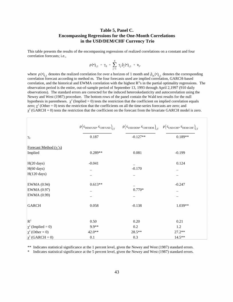
43

ρ (•)t,1 γ0 4


Table 5, Panel C.Encompassing Regressions for the One-Month Correlations



where denotes the realized correlation for over a horizon of 1 month and denotes the correspondingρ (•)t,1 ρm(•)t,1correlation forecast according to method m. The four forecasts used are implied correlation, GARCH-basedcorrelation, and the historical and EWMA correlation with the highest R2's in the partial optimality regressions. Theobservation period is the entire, out-of-sample period of September 13, 1993 through April 2,1997 (910 dailyobservations). The standard errors are corrected for the induced heteroskedasticity and autocorrelation using theNewey and West (1987) procedure. The bottom rows of the panel contain the Wald test results for the nullhypothesis in parentheses.χ2 (Implied = 0) tests the restriction that the coefficient on implied correlation equalszero;χ2 (Other = 0) tests the restriction that the coefficients on all the time-series forecasts are zero; andχ




γ0 0.187 -0.127** 0.189**

Forecast Method (γj’s)Implied 0.289** 0.081 -0.199

H(20 days) -0.041 _ 0.124H(60 days) _ -0.170 _H(120 days) _ _ _

EWMA (0.94) 0.613** _ -0.247EWMA (0.97) _ 0.770* _EWMA (0.99) _ _ _

GARCH 0.058 -0.138 1.039**

R2 0.50 0.20 0.21χ

2 (Implied = 0) 9.9** 0.2 1.2χ

2 (Other = 0) 42.0** 28.5** 27.2**χ

2 (GARCH = 0) 0.1 0.3 14.5**


44

ρ (•)t,3 γ0 4


Table 5, Panel D.Encompassing Regressions for the Three-Month Correlations



where denotes the realized correlation for over a horizon of 3 months and denotes the correspondingρ (•)t,3 ρm(•)t,3correlation forecast according to method m. The four forecasts used are implied correlation, GARCH-basedcorrelation, and the historical and EWMA correlation with the highest R2's in the partial optimality regressions. Theobservation period is the entire, out-of-sample period of September 13, 1993 through April 2,1997 (910 dailyobservations). The standard errors are corrected for the induced heteroskedasticity and autocorrelation using theNewey and West (1987) procedure. The bottom rows of the panel contain the Wald test results for the nullhypothesis in parentheses.χ2 (Implied = 0) tests the restriction that the coefficient on implied correlation equalszero;χ2 (Other = 0) tests the restriction that the coefficients on all the time-series forecasts are zero; andχ




γ0 0.362 -0.195** 0.391**

Forecast Method (γj‘s)Implied 0.335** 0.043 -0.349**

H(20 days) -0.135 _ -0.029H (60 days) _ -0.312 _H (120 days) _ _ _

EWMA (0.94) 0.570** _ 0.029EWMA (0.97) _ 0.946** _EWMA (0.99) _ _ _

GARCH -0.155 0.496** 0.686**

R2 0.37 0.25 0.14χ

2 (Implied = 0) 11.0** 0.1 7.3**χ

2 (Other = 0) 28.6** 77.8** 24.1**χ

2 (GARCH = 0) 0.2 7.9** 15.6**


45

ρ (•)t,1 γ0 4

j1γj ρj (•)t,1,

Table 6.Encompassing Regressions for the One-Month Correlation

between the DEM and the JPY measured in USD: Subsamples


where denotes the realized correlation for over a horizon of 1 month and denotes the correspondingρ (•)t,1 ρm(•)t,1correlation forecast according to method m. The four forecasts used are implied correlation, GARCH-basedcorrelation, and the historical and EWMA correlation with the highest R2's in the partial optimality regressions. Theobservation period is the entire, out-of-sample period, but broken into eight non-overlapping subsamples of roughly200 observations each. The standard errors are corrected for the induced heteroskedasticity and autocorrelationusing the Newey and West (1987) procedure.

γ0 γImplied γH(60) γE(0.97) γGARCH R2

A. October 2, 1990 – July 8, 1991 (200 observations)

0.471** 0.507** 0.692** -1.308** 0.547** 0.43

B. July 9, 1991 – April 13, 1992 (200 observations)

0.897** -0.124 -0.624 0.425 -0.047 0.05

C. April 14, 1992 – January 18, 1993 (200 observations)

0.893** 0.349** 0.736 -3.078** 1.727** 0.24

D. January 19, 1993 – October 25, 1993 (200 observations)

0.099 0.979* -0.578 0.046 -0.030 0.10

E. October 26, 1993 – August 1, 1994 (200 observations)

0.365 -0.118 -0.485 1.870* -0.763 0.51

F. August 2, 1994 – May 9, 1995 (200 observations)

2.031** -0.061 -1.249** -0.670 0.188 0.43

G. May 10, 1995 – February 21, 1996 (200 observations)

0.529 -0.429 0.086 -0.046 0.645 0.15

H. February 22, 1996 – April 2, 1997 (279 observations)

0.996** -0.419 -0.561 0.894 -0.654 0.07** Indicates statistical significance at the 1 percent level, given the Newey and West (1987) standard errors.* Indicates statistical significance at the 5 percent level, given the Newey and West (1987) standard errors.

is implied correlation worth calculating? · is implied correlation worth calculating? ... exchange...

Documents