IS HIGHER-QUALITY LAND DEVELOPED

EARLIER?

Juan Carlos Lopez∗and Richard Arnott†

JEL Codes: R14, R31

Keywords : Land Use Patterns, Housing Supply and Markets

April 24, 2018

∗Department of Economics, University of Denver, Denver CO 80208 juancarlos.lopez@du.edu†Department of Economics, University of California, Riverside CA 92506 richard.arnott@ucr.edu

1

Abstract

This paper addresses the question: Is higher-quality land developed earlier? To

answer this question, the paper applies comparative static analysis to the Arnott-

Lewis model of the transition of land from agricultural to urban use. Four dimen-

sions of land quality are considered: agricultural fertility, land preparation costs,

structure construction costs, and amenities. It is shown that: i) an increase in

agricultural fertility increases structural density and delays development; ii) a de-

cline in land preparation cost reduces structural density and hastens development;

iii) both an increase in amenities and a decrease in structure construction costs

normally hasten development, but in anomalous cases can delay development. The

paper presents two numerical examples illustrating these anomalies, and explains

them.

2

1 Introduction

In a typical introductory lecture in land economics, a distinction is made between the

Ricardian model of land use, rent and value and the corresponding von Thunen model.

The Ricardian model focuses on the intrinsic properties of land, including fertility and

natural amenities, which may be referred to collectively as “land quality”. The von

Thunen model, in contrast, focuses on differences in accessibility. Courses in urban

economics focus on the monocentric city model, which extends the von Thunen model

to the urban context. The monocentric model has been analyzed exhaustively (and

some would argue exhaustingly). Ricardian differences in land are discussed, and indeed

feature prominently in hedonic analysis. Remarkably, however, it appears that Ricardian

differences in land have not been systematically incorporated into the monocentric city

model. The aim of this paper is to at least partially remedy this oversight by addressing

the question: “Is higher-quality land developed (in urban use) earlier?” The answer to

the question depends, of course, on what is meant by land quality. We consider four

dimensions of land quality: fertility, natural amenities, land preparation costs (so that

servicing of the land is cheaper on higher quality land), and structure construction costs

(so that structures are cheaper to construct on higher quality land).

There are static and dynamic variants of the monocentric city model. In the more

familiar static variant, structures are treated as mobile and perfectly malleable. A parcel

of land is in urban use if its rent in urban use exceeds its agricultural rent, and its floor-

area ratio or structural density is determined by its urban rent. Over time, as the urban

rent at a particular location increases, structural density increases. While we address the

paper’s question in the context of the static variant of the monocentric city model at the

end of the paper, it is not the paper’s focus. Instead, we focus on a dynamic variant of

the monocentric city model in which structures are durable. In this situation, the owner

of a parcel of land that has not yet been developed in urban use faces the decisions of

when and at what structural density to convert the parcel to urban use. To simplify

the model as much as possible, we make the assumption that structures are immutable

and indestructible (so that, when a site is developed, the structure that is built on the

site cannot be altered) and of constant quality. Furthermore, in our analysis we consider

3

parcels that are equally accessible. The answers to the paper’s question can then be

provided by comparative static analysis applied to the Arnott and Lewis (1979) model

of the transition of land to urban use.

Intuitively, the answer depends on what dimension of land quality is considered. One

obvious intuition is that, ceteris paribus, parcels with lower fertility are developed earlier

since the opportunity cost of their being developed is lower. Another obvious intuition

is that parcels for which the marginal cost of construction is higher are developed either

later or at lower density or both. The durability of structures makes the comparative

statics result more complicated because the land quality affects two margins of choice:

the timing and the density of development. How those two margins interact may depend

in quite a complicated way on factors such as the interest rate, the growth rate of rents,

and the elasticity of substitution between land and capital in the production of structures.

In the urban and regional economics literature there has been some recognition that

land heterogeneity plays a role in determining urban spatial structure. Burchfield et al.

(2006) use satellite data on US metropolitan areas to explore differences in sprawl across

regions between 1976-1992. As part of their set of explanatory variables they consider the

effect of heterogeneity in temperature, physical terrain and access to aquifers. The authors

conclude that physical geography accounts for 25 percent of the variation in sprawl over

US metropolitan areas. Saiz (2010) explores how variation in developable land due to

geographic constraints across US metropolitan areas affects housing supply elasticities.

He finds that land-constrained cities have significantly lower supply elasticities and higher

housing prices than cities with a greater availability of developable land. In a different

vein, Irwin and Bockstael (2002) consider how the development decision for a parcel

of land in a current time period is influenced by spatial externalities associated with

the land use decisions from neighboring plots in previous periods. The authors develop a

dynamic model of interacting agents which yields a more fragmented development pattern

in exurban areas than would be predicted by the standard monocentric model.

Section 2 presents the dynamic model with immutable and indestructible structures.

Section 3 provides the results of the comparative static exercises for different forms of

land quality. Section 4 remarks on the previous three sections. Section 5 treats the easier

4

but less realistic static model. And section 6 concludes.

2 The Dynamic Model

The dynamic model is a variant of the Arnott-Lewis model. A profit-maximizing

landowner decides when and at what density to convert a unit area of land he owns

from agricultural to urban use, in the absence of zoning restrictions. To simplify, we

assume that the interest rate, the growth rate of urban rent (per unit floor area), and

the agricultural rent remain constant over time. Furthermore, we ignore the quality

dimension of structures, including depreciation. Finally, we augment Arnott-Lewis to

allow for (fixed) land preparation (or servicing) costs. The component of land servicing

costs that increases in structural density is treated through the construction cost function.

We employ the following notation:

s structural density (or floor-area ratio)

T timing of development

q quality of land, whose interpretation varies depending on the typeof quality differentiation being considered

S(s, q) current floor rent per unit area of land, which depends on s and onq only when q represents natural amenities

r interest/discount rate

g growth rate of floor rent

C(s, q) current structure construction cost per unit area of land, whichdepends on s and on q only when q represents elements of the landthat affect structure construction costs

L(q) current land preparation (servicing) cost per unit area of land,which depends on q only when q represents elements of the landthat affect land preparation costs

R(q) agricultural rent, which depends on q only when q represents agri-cultural fertility

π(s, T, q) present value of profit per unit area of land

Note that an improvement in natural amenities may affect floor rent differently on dif-

ferent floors of a building; for example, a view of the ocean may be visible for floors

5

above a certain level but not below it. Similarly, an improvement in land quality may

affect construction costs differently for different floors; for example, bedrock may have no

effect on the construction costs for buildings below a certain floor-area ratio but reduce

construction costs for building above that floor area.

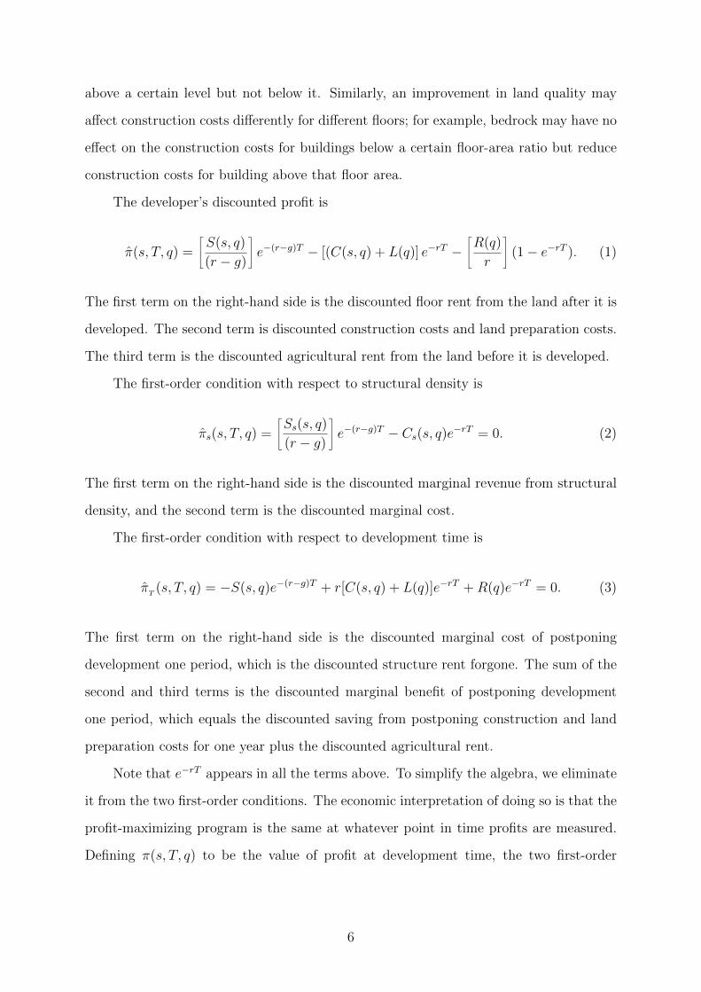
The developer’s discounted profit is

π(s, T, q) =

ñS(s, q)

(r − g)

ôe−(r−g)T − [(C(s, q) + L(q)] e−rT −

ñR(q)

r

ô(1− e−rT ). (1)

The first term on the right-hand side is the discounted floor rent from the land after it is

developed. The second term is discounted construction costs and land preparation costs.

The third term is the discounted agricultural rent from the land before it is developed.

The first-order condition with respect to structural density is

πs(s, T, q) =

ñSs(s, q)

(r − g)

ôe−(r−g)T − Cs(s, q)e

−rT = 0. (2)

The first term on the right-hand side is the discounted marginal revenue from structural

density, and the second term is the discounted marginal cost.

The first-order condition with respect to development time is

πT(s, T, q) = −S(s, q)e−(r−g)T + r[C(s, q) + L(q)]e−rT +R(q)e−rT = 0. (3)

The first term on the right-hand side is the discounted marginal cost of postponing

development one period, which is the discounted structure rent forgone. The sum of the

second and third terms is the discounted marginal benefit of postponing development

one period, which equals the discounted saving from postponing construction and land

preparation costs for one year plus the discounted agricultural rent.

Note that e−rT appears in all the terms above. To simplify the algebra, we eliminate

it from the two first-order conditions. The economic interpretation of doing so is that the

profit-maximizing program is the same at whatever point in time profits are measured.

Defining π(s, T, q) to be the value of profit at development time, the two first-order

6

conditions may be written as

πs(s, T, q) =

ñSs(s, q)

(r − g)

ôegT − Cs(s, q) = 0, (4)

πT(s, T, q) = −S(s, q)egT + r[C(s, q) + L(q)] +R(q) = 0. (5)

To simplify notation, we define B(s, q) ≡ r[C(s, q) +L(q)] +R(q), to be the contempora-

neous benefit from postponing development for a unit of time, which equals the interest

on the construction and land preparation costs, plus the agricultural rent from land. The

first-order condition with respect to T can then be rewritten as

πT(s, T, q) = −S(s, q)egT +B(s, q) = 0. (6)

Sufficient conditions for (4) and (5) to describe a local profit maximum are that

πss(s, T, q) = Sss(s, q)egT/(r − g) − Css(s, q) < 0, π

TT(s, T, q) = −g[S(s, q)]egT < 0, and

πss(s, T, q)πTT(s, T, q) − π

sT(s, T, q)πTs(s, T, q) > 0. The first condition is that there are

decreasing marginal profits to constructing floor area. The second condition is that rents

are growing. Since πsT

(s, T, q) = πTs

(s, T, q) = g[Ss(s, q)/(r − g)]egT > 0, the third

condition may be rewritten as πTT

(s, T, q)/πTs

(s, T, q) = (ds/dT )FOCs < (ds/dT )FOCT=

πsT

(s, T, q)/πss(s, T, q), which states that in T − s space, the slope of the first-order con-

dition with respect to T is steeper than that with respect to s (both slopes are positive).

Were it not for R(q), the condition would have the economic interpretation that the

elasticity of substitution between land and capital in the production of a structure is less

than one. If the condition does not hold, the point at which the two first-order conditions

intersect is a local minimum; profit can be increased either by building earlier at a lower

density or building later at a higher density.

Figure 1 plots the two first-order conditions, FOCs and FOCT , in T–s space. Suffi-

cient conditions for their point of intersection to characterize a local profit maximum are

that the two first-order conditions be positively sloped, and that the first–order condition

with respect to T is steeper than that with respect to s.

7

FOCT

FOCs

T

s

Figure 1: First-order conditions in T − s space

3 Comparative Static Analysis

3.1 Laying the groundwork

We shall logarithmically differentiate (4) and (6). The advantage of logarithmic

differentiation is that all terms are expressed in unitless quantities such as elasticities.

Since the process of logarithmic differentiation is not covered in many of today’s graduate

programs, we proceed step by step. First, totally differentiate (4) and (6) with respect

to s, T , and q, holding the parameters r and g constant, where to simplify notation we

suppress the arguments of the functions,ñSss

(r − g)egT − Css

ôds+

ñgSs

(r − g)egTôdT =

ñ− Ssq

(r − g)egT + Csq

ôdq, (7)ñ

gSs

(r − g)]egTôds+

î−gSe−gT

ódT =

îSqe

−gT −Bq

ódq, (8)

and where use is made of the fact that πTs

= −Ss(s, q)egT +Bs(s, q) = gSs(s, q)e

gT/(r−

g) = πTs

. Next divide each term by the corresponding term in the equation that was

totally differentiated. For example, to obtain Css in the first equation, the term Cs was

differentiated. Using the relationships derived from the first-order conditions in (4) and

8

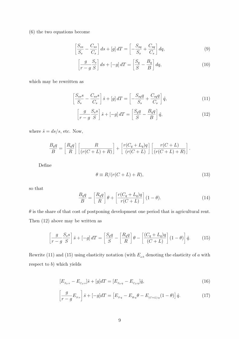
(6) the two equations becomeñSss

Ss

− Css

Cs

ôds+ [g] dT =

ñ−Ssq

Ss

+Csq

Cs

ôdq, (9)ñ

g

r − gSs

S

ôds+ [−g] dT =

ñSq

S− Bq

B

ôdq, (10)

which may be rewritten asñSsss

Ss

− Csss

Cs

ôs+ [g] dT =

ñ−Ssqq

Ss

+Csqq

Cs

ôq, (11)ñ

g

r − gSss

S

ôs+ [−g] dT =

ñSqq

S− Bqq

B

ôq, (12)

where s = ds/s, etc. Now,

Bqq

B=

ñRqq

R

ô ñR

(r(C + L) +R)

ô+

ñr(Cq + Lq)q

(r(C + L)

ô ñr(C + L)

(r(C + L) +R)

ô.

Define

θ ≡ R/(r(C + L) +R), (13)

so that

Bqq

B=

ñRqq

R

ôθ +

ñr(Cq + Lq)q

r(C + L)

ô(1− θ). (14)

θ is the share of that cost of postponing development one period that is agricultural rent.

Then (12) above may be written asñg

r − gSss

S

ôs+ [−g] dT =

ñSqq

S−ñRqq

R

ôθ −

ñ(Cq + Lq)q

(C + L)

ô(1− θ)

ôq. (15)

Rewrite (11) and (15) using elasticity notation (with Ea:b

denoting the elasticity of a with

respect to b) which yields

[ESs:s− E

Cs:s]s+ [g]dT = [E

Ss:q− E

Cs:q]q, (16)ñ

g

r − gE

S:s

ôs+ [−g]dT =

îE

S:q− E

R:qθ − E

(C+L):q(1− θ)

óq. (17)

9

Putting the set of linear equations in matrix form we then have

U V

X Y

sdT

=

WZ

q, (18)

where

U = ESs:s− E

Cs:s< 0, (19)

V = g > 0, (20)

W = −ESs:q + ECs:q

R 0, (21)

X =g

r − gES:s > 0, (22)

Y = −g < 0, (23)

Z = ES:q − θER:q − (1− θ)E(C+L):q

R 0. (24)

Finally, solving out the pair of simultaneous linear equations using Cramer’s Rule gives

s

q=

(WY − V Z)

(UY − V X), (25)

dT

q=

(UZ −WX)

(UY − V X). (26)

For Eqs. (19)-(24) we have indicated the signs of the various terms. The signs of W

and Z depend on elasticities with respect to land quality, which depend on the nature

of land quality, and are therefore a priori ambiguousÄR 0ä. Since we are considering

land that has not yet been developed at the present time, which we have normalized to

zero, T is positive. Finally, we assume that, as functions of structural density, there are

increasing marginal costs to construction, ECs:s

> 0.

10

Define

∆ = UY − V X (27)

= g[−(ESs:s− E

Cs:s)− g

r − gE

S:s].

The third of the second-order conditions requires that ∆ be positive.

An increase in land quality causes either or both of the first-order conditions, (4) and

(5), to shift. The nature of land quality determines which of the first-order conditions is

shifted and by how much. This is the subject of the subsections that follow. We consider

only one type of land quality at a time.

3.2 An improvement in land quality corresponds to an increase

in agricultural fertility

This is the simplest case to treat. Since quality is an ordinal concept, we may

cardinalize it as we wish. Here the simplest cardinalization is to measure land quality as

agricultural fertility, i.e. R(q) = q. In which case ER:q

= 1. Since only one type of land

quality is considered at a time, ES:q

= ECs:q

= E(C+L):q

= 0. We then obtain

s

q=θg

∆> 0, (28)

dT

q= −

θ[ESs:s− E

Cs:s]

∆> 0. (29)

With respect to Fig. 1, an increase in agricultural fertility has no effect on FOCs

and causes FOCT to shift to the right (since holding structural density fixed, profit-

maximizing development time increases). Thus, more fertile land is developed later and

at higher density, as argued earlier.

11

3.3 An improvement in land quality corresponds to a decrease

in the fixed cost of servicing land per unit area

In this section we employ a different normalization of land quality in which land

servicing cost is inversely proportional to quality, i.e. L(q) = L/q. Thus, W = 0 and

Z = −(1 − θ)E(C+L):q

= −(1 − θ)[d(C + L(q))/dq]q/(C + L) = (1 − θ)L/(C + L). We

obtain:

s

q= −g(1− θ)L

(C + L)

1

∆< 0, (30)

dT

q= −

(1− θ)L(ESs:s− E

Cs:s)

(C + L)

1

∆< 0. (31)

With respect to Fig. 1, a decrease in (fixed) land servicing costs has no effect on FOCs and

causes FOCT to shift to the left (since holding structural density fixed, profit-maximizing

development time decreases). Thus, a decrease in land servicing costs causes development

to occur earlier and at lower density.

3.4 An improvement in land quality corresponds to a decrease

in construction costs

The first-order condition with respect to structural density depends on marginal

construction cost, while the timing condition depends on total or average construction

cost. Thus, we should expect that the manner in which a decrease in construction costs

affects development timing and density depends on the way in which a marginal increase

in quality affects the construction cost function. For example, higher-quality land may

correspond to land that is less prone to flooding or to land that is further from a seismic

fault, and the change induced in the cost-minimizing construction technology may be

quite different in the two situations. One might cause a proportional change in construc-

tion cost at all other densities, while the other might cause a decrease in construction

cost only for structural densities above a certain level.

We shall first present the intuition for our results, drawing on Figure 1. We shall

then work through the algebra, and present an example in which an improvement in land

12

quality results in later development. This result is of particular interest since it runs

counter to most of our results (higher land quality corresponding to greater agricultural

fertility being the exception) in which the improvement in land quality results in earlier

development by decreasing the marginal benefit from postponing development.

A decrease in construction costs causes the first-order condition with respect to

development timing to shift left and the first-order condition with respect to structural

density to shift up. As noted above, the amount by which the timing first-order condition

shifts left depends on how land quality improvement affects average cost, while the amount

by which the density condition shifts up depends on how land quality improvement affects

marginal cost. In the algebra that follows, we shall present two main results. The first

provides a point of reference. In a particularly simple variant of the model in which

agricultural rent and land improvement costs are zero, a land quality improvement that

results in an equiproportional reduction in construction costs at all densities results in

earlier development with no change in density. The second result is that a land quality

improvement that reduces marginal construction cost proportionally more than it reduces

average construction cost can result in later development.

The intuition is as follows. Consider two neighboring sites that differ only in land

quality. Suppose that it is profit maximizing to develop site 1 10 years from now at

20 stories. Site 2 differs from site 1 in having bedrock underneath. We consider two

situations. In the first, the bedrock foundation results in an equiproportional reduction

in construction costs at all densities. For FOCT , holding structural density fixed, lower

construction costs reduce the benefit from postponing construction, encouraging earlier

development. For FOCs, holding development time fixed, lower construction costs reduce

the marginal cost of density, encouraging development at higher density. In the reference

situation in which construction costs for site 2 are lower than those for site 1 in the same

proportion at all densities, the amount by which FOCT for site 2 lies to the left of that

for site 1 relative to the amount by which FOCs for site 2 lies above that for site 1 is

such that development on site 2 occurs at 20 stories as well but earlier than on site 1.

Now modify the example so that the bedrock foundation permits the use of a con-

struction technique that reduces construction costs only above 30 stories. Since FOCs

13

depends on marginal cost, the bedrock foundation has no effect on FOCs below 30 sto-

ries, but above 30 stories causes FOCs to shift up discontinously. Since FOCT depends

on average cost, having the bedrock foundation has no effect on FOCT up to 30 stories

but above that causes its slope to increase (rather than to shift up discontinuously). For

site 2, there may then be two local maxima, and profit may be higher with construction

at 30 rather than 20 stories. But rents ten years from now may not be sufficiently high

to justify construction at the higher density, so that development is postponed.

We now turn to the algebra. Because of the type of land quality improvement being

considered, Lq = 0, so that E(C+L):q

= Cqq/(C + L) = EC:q

(C/(C + L)). In addition

W = ECs:q

and Z = −(1− θ)E(C+L):q

. Then

s

q= g

[−E

Cs:q+ (1− θ)E

C:q

C(C+L)

]∆

, (32)

dT

q=

[−(1− θ)(E

Ss:s− E

Cs:s)E

C:q

C(C+L)

− ( gr−gES:s

)ECs:q

]∆

. (33)

We present two results. The first formalizes the argument presented above for the

first situation. The second gives an example of the second situation in which an increase

in land quality that lowers marginal construction costs more than average construction

costs results in construction being delayed.

Result 1: If there are no land improvement costs (so that L = 0), if agricultural rent

is zero (so that R = 0), and if higher-quality land corresponds to an an equiproportional

reduction in construction costs for all levels of density (so that C(s, q) = C(s)f(q), with

q > 0, f > 0 and f ′ < 0) then s/q = 0 and dT/q < 0.

Proof. Under the stated conditions, EC:q = ECs:q = f ′q/f , so that (32) and (33) reduce

to

s

q=g(−E

Cs:q+ E

C:q)

∆= 0,

dT

q=−(E

Ss:s− ECs:s)EC:q − ECs:q(

gr−gES:s

)

∆= (f ′q/f)

−(ESs:s− ECs:s)− ( g

r−gES:s)

∆.

14

Recalling that ∆ = g[−(ESs:s− ECs:s)− ( g

r−gES:s)], the expression for dT/q reduces to

dT

q=

(f ′q/f)

g< 0.

Thus, when ∆ > 0, the improvement in quality causes profit-maximizing construction to

be brought forward.

The last equation follows directly from the first-order conditions. Under the stated

conditions, the first-order conditions remain satisfied if egT/f(q) is equal to a constant.

Total differentiation gives gdT − (f ′/f)dq = 0 so that dT/q = (f ′q/f)/g.

Result 2: If there are no land improvement costs (so that L = 0), if agricultural

rent is zero (so that R = 0), if rent per unit floor area is independent of density (so that

S(s) = ps), and if higher land quality results in a reduction in construction costs that

is proportionally higher at higher densities, then it may be profitable to develop higher

quality land later.

Proof. The proof entails the construction of a numerical example. We assume a con-

struction cost function of the form C(s, q) = sbeas/q , where a > 0 and b > 0. This cost

function has the property that an increase in land quality results in a greater proportional

reduction in construction costs the higher is structural density (i.e., C/q = −as/q2). The

partial derivatives of this cost function are

Cs = C(b/s+ a/q),

Css = Cs(b/s+ a/q)− Cb/s2 = C((b/s+ a/q)2 − b/s2),

Cq = −asC/q2,

Csq = −aC/q2 − asCs/q2 = −(aC/q2)(1 + b+ as/q).

We shall choose other parameters such at s = 1 and T = 0 at the optimum, and normalize

such that q = 1 in the base situation. Then at the base optimum Cs/C = b + a,

Css/Cs = ((b+ a)2 − b)/(b+ a), Cq/C = −a, and Csq/Cs = −a(1 + b+ a)/(b+ a).

15

Under the stated conditions, the first-order conditions are

s : pegT − (r − g)Cs(s, q) = pegT − (r − g)sbeas/q(b/s+ a/q) = 0,

T : −psegT + rC(s, q) = −psegT + rsbeas/q = 0.

These conditions are satisfied at q = s = 1 and T = 0 if

p− (r − g)ea(b+ a) = 0, −p+ rea = 0, (34)

and in particular with the parameters p = rea and (r − g)(b + a) = r, which we assume

to hold.

The example satisfies the second-order conditions that πss < 0 and πTT

< 0. To

establish the Result, it remains to prove that ∆ > 0 and dT/q > 0. Now, under the

stated conditions, ES:s = 1 and ESs:s = 0, so that ∆ = g(ECs:s − g/(r − g)). Since

ECs:s = [(b+ a)2 − b]/(b+ a), from (34), g/(r− g) = r/(r− g)− 1 = b+ a− 1, it follows

that ∆ = g(ECs:s − g/(r − g)) = b + a − b/(b + a) − (b + a) + 1 = a/(a + b) > 0. By a

similar line of reasoning

dT

q=

[ECs:s

EC:q− E

Cs:q( gr−g )]

g(ECs:s− g

r−g )

=a

a+b((1 + b+ a) g

r−g − ((b+ a)2 − b))gÄ

aa+b

ä=

(g

r−g − a)

g,

where use is made of the parameter restrictions in (34). It follows directly that if a <

g/(r − g), dT/dq > 0.

Consider an example in which a = 1, and g/r = 2/3 implying that dT/q = 1/g.

Suppose g = 0.02, then a 10% improvement in land quality would result in construction

occurring five years later.

16

3.5 An improvement in land quality corresponds to an increase

in amenities

Define the reference situation to occur when S(s, q) = sp(q) so that the floor rent on

all stories is the same, and an increase in amenities results in a uniform increase in the

floor rent on all stories. In this reference situation, (25) and (26) reduce to

s

q= g

(ESs:q − ES:q)

∆= 0, (35)

dT

q=

[(ESs:s − ECs:s)ES:q + ESs:q(g

r−gES:s)]

∆(36)

=(p′q/p)[−ECs:s + g

r−g ]

∆= −(p′q/p)

g< 0,

with

∆ = g[−ESs:s + ECs:s −g

r − gE

S:s] = g[ECs:s −

g

r − g].

Thus, with ∆ > 0 the increase in amenities results in earlier development at unchanged

density. These results have a straightforward explanation. In the above specification, an

increase in amenities changes the developer’s problem only in that the future is brought

forward; it is profit maximizing for the developer to do exactly as he would have done

before the amenity improvement, but earlier. In particular, q and T are related that such

that p(q)egT is constant, so that dT/q = −(p′q/p)g.

We now investigate whether, with the general specification of the rent function,

S(s, q), it is possible for an increase in amenities to result in a postponement of de-

velopment. Intuitively for this to occur, the increase in amenities must increase rents

disproportionately at higher density. Imagine a situation in which there are two sites,

site 1 and site 2. It is profit maximizing to develop site 1 at 20 stories today. Site 2

differs from site 1 only in that it has an unobstructed view of the mountains above 30

stories. Rents today however are not sufficiently high to justify constructing a building

of this height. It may however be profit maximizing to delay development of site 2 until

building above 30 stories is justified.

We assume a particular rentals function, and derive restrictions on the construction

17

cost function such that an increase in amenities causes development to be delayed. The

assumed form of the rentals function is S(s, q) = m(s/q + s2q2), with m > 0, and the

parameters are such that, with q = 1, the profit maximum occurs with s = 1 and at

T = 0. Rent is higher on higher stories (at the profit maximum with s = 1, ESs:s = 2/3)

and is proportionally higher the higher the level of amenity (dESs:s/dq > 0). With this

rentals function,

ES:s

= (1/q + 2sq2)/(1/q + sq2),

ESs:s

= 2sq2/(1/q + 2sq2),

ES:q

= (−s/q + 2s2q2)/(s/q + s2q2),

ESs:q

= (−1/q2 + 4q2)/(1/q + 2sq2).

Substituting these elasticities, evaluated at q = 1 and s = 1, gives the following expression

for ∆ and the numerator of dT/q, which we define as N , from (26):

∆ = −gÇÇ

2

3− ECs:s

å+

3

2

g

r − g

å= −g

Ç2

3− ECs:s +

3

2

g

r − g

å, (37)

N =

Ç1

2

Ç2

3− ECs:s

å+

3

2

g

r − g

å=

1

2

Ç2

3− ECs:s + 3

g

r − g

å. (38)

Both ∆ and N must be positive for the second-order condition to be satisfied and for an

increase in amenities to delay profit-maximizing development. Solving (37) and (38) for

∆ > 0 and N > 0 yields

2

3+

3

2

g

r − g< E

Cs:s<

2

3+ 3

g

r − g. (39)

Consider the case where g/r = 1/2, in which case g/(r−g) = 1 and 13/6 < ECs:s

< 22/6.

Suppose ECs:s

= 3, which falls in the appropriate range. This yields dT/q = 2/(5g). With

a rental growth rate of 2% then a 10% increase in amenities yields a development delay

of 2 years.

18

4 Remarks

1. We came to the question posed in the paper’s title indirectly. Arnott was in-

terested in the empirical validity of the Henry George Theorem. The static version of

the Theorem is that, in an efficient metropolitan area (including the efficient population

size), aggregate urban land rent and the revenue raised from the marginal cost pricing

of urban public services just cover the costs of providing the efficient level of public ser-

vices; thus, the single tax that would be needed to finance public services would be a

confiscatory tax of urban land rent. The dynamic version of the Theorem is that, in

an efficient metropolitan area, aggregate urban land value plus the discounted revenue

raised from the marginal cost pricing of public services just cover the discounted costs of

providing the efficient level of public services. Since metropolitan areas are not efficient,

one should not expect the Henry George Theorem to hold exactly. Nonetheless, it is of

interest to investigate the empirical magnitude of aggregate land values in a metropolitan

area. Arnott had data, assembled by the Southern California Association of Governments

(SCAG) from land registry records on the sales price, year of sale, and location and area

of all vacant land parcels in the five-county Greater Los Angeles area, but no data on

the Ricardian properties of the parcels, except for distance from the ocean. The data are

sufficient to estimate a market land value surface for vacant land over the metropolitan

area (Zhang and Arnott, 2015). Arnott posed this question: Is it sound to estimate the

aggregate market value of all land, both vacant and developed, as the volume under this

land value surface? Put alternatively, in a small geographic area, does the mean market

value of vacant land per unit area provide an unbiased estimate of the mean market value

of developed land per unit area? This is not the place to provide a detailed discussion

of all the issues1. But one issue is whether, in a small geographic area, higher-quality

land is systematically developed earlier than lower-quality land. If it is, then, in each

small geographic area, the mean value of vacant land per unit area provides a systematic

underestimate of the mean value of developed land per unit area. It was an investigation

1 Suffice it to say that three of the issues are zoning, the plattage effect (that, over each smallgeographic area, the value of land per unit area is higher for smaller than for larger lots), and theagglomeration benefits from proximity to other developed (and perhaps undeveloped) land valuesthat are captured in land rents and values.

19

of this issue that motivated this paper’s analysis.

Arnott had another motivation for writing the paper. Land is an ideal tax base. A

tax on land would not only be efficient, but would also likely have desirable distributional

impacts. But given the propensity of taxpayers to appeal assessments, it is important

to get accurate assessments of land values. Unfortunately, the analysis of this paper

indicates that estimating the value of developed land from the sales prices of proximate

vacant parcels is problematic, when, as is normally the case, higher quality land parcels

get developed earlier.

2. We believe the model used to investigate the question that is the title of this paper, as

well as our analysis of its properties are sound. However, the model provides a simplified

description of reality, as indeed do all models, and should be regarded as providing a

starting point for further, more sophisticated analyses. There are many ways in which

the model can be enriched to improve its realism, including treating uncertainty (and

along with it the option value component of vacant land) and risk aversion, zoning,

depreciation of structures, taxes, structural quality, and redevelopment. Furthermore,

two of the model’s simplifying assumptions, that the growth rate of rents and the interest

rate are constant over time, can be relaxed.

3. It is disappointing that the empirical literature in real estate economics has paid

little attention to developers’ decisions of when and at what density to build, since these

decisions affect the properties of metropolitan real estate and construction cycles, and the

impact of tax, land use, and other policy changes on them. The theory presented in this

paper assumes that these decisions are determined completely by market forces (if there is

zoning, then it is non-binding). If, at the other extreme, developers’ construction timing

and development decisions are fully determined by zoning regulations, then metropolitan

real estate models should contain a module that endogenizes zoning regulations (the

political economy of zoning).

4. The paper considered only one dimension of quality differentiation at a time. However,

adjacent plots of land may differ in more than one dimension simultaneously. For example,

if one site lies higher on a hillside than another, it will have a better view but at the same

time its land preparation and construction costs may be higher.

20

5 The Static Model

The static model of metropolitan land use is the monocentric city model. It has three

dynamic interpretations. The first is that structures are non-durable, so that each day

the landowner decides on structural density so as to maximize that period’s profits based

on current conditions; the second is that structures are durable but mobile, so that the

landowner decides how much structure capital to rent every day; and the third is that the

metropolitan area is in a steady-state, so that the economic cost of operating a unit area

of land in urban use equals the opportunity cost of the land (the agricultural rent) and

the durable capital (the cost of capital)2. In each of these interpretations, the landowner

chooses whether to operate his land in agricultural use or in urban use, and if he chooses

to operate it in urban use, he chooses structural density. The agricultural rent and the

rent per unit floor area are based on market clearing in the location-specific markets, and

the cost of capital is taken as exogenous. In keeping with the durable structures model,

the cost of capital is taken to be the interest rate. Where the same notation is employed

as in the previous section, conditional on operating his land in urban use, the landowner’s

profit-maximization problem is

maxs

S(s, q)− rC(s, q)− rL(q). (40)

The first-order condition with respect to s is

Ss(s, q)− rCs(s, q) = 0. (41)

Structural density is chosen such that the marginal revenue of structural density equals

the marginal cost. Letting s∗(q) be the profit-maximizing structural density, the urban

land rent on land of quality q is U(q) = S(s∗(q), q)− rC(s∗(q))− rL(q). The landowner

operates his land in urban use if the urban land rent, U(q), exceeds the agricultural

land rent, R(q), and in agricultural use if the inequality is reversed. Thus, land quality

determines whether land is operated in urban or agricultural use, and, conditional on

2 There is a model that is intermediate between the durable and non-durable structure models. Prop-erty owners may irreversibly add storeys to their buildings, as is done in desert climates.

21

being operated in urban use, also determines the structural density.

Let q# denote the quality of land at which the landowner is indifferent between

operating his land in urban and agricultural use. It is given implicitly by the equation

U(q#) = R(q#). (42)

Where q represents agricultural fertility, we have that land of quality higher than q# is

operated in agriculture and that land of quality lower than q# is operated in urban use.

Where higher q corresponds to better amenities, corresponding to which is a higher urban

rent or to reduced land preparation and construction costs, we have the opposite result.

To make operational the concept of development time in this model, we assume, as

we did with the durable housing model, that urban rents grow faster than the agricultural

rent, and we define development time to be the first time at which a parcel of land is

operated in urban use. Then, where q represents agricultural fertility, we have that higher-

quality land is developed later. And where higher q corresponds to better amenities or

to reduced construction costs, we have that higher quality land is developed earlier.

Finally, we generate results relating profit-maximizing structural density, conditional

on land being more profitably employed in urban use, to land quality, by differentiating

(21):

ds∗(q)

dq=Ssq(s

∗, q)− rCsq(s∗, q)

Sss(s∗, q)− Css(s∗, q). (43)

We assume that there is increasing marginal cost to structural density. Then:

• Where higher-quality land corresponds to greater agricultural fertility,

ds∗(q)/dq = 0.

• Where higher-quality land corresponds to lower land preparation costs, which are

interpreted as a lower fixed cost of construction, ds∗(q)/dq = 0.

• Where higher-quality land corresponds to improved amenities, ds∗(q)/dq > 0.

• Where higher-quality land corresponds to lower marginal construction costs,

ds∗(q)/dq > 0.

22

Thus, the results from the static model are very similar to those from the dynamic

model with durable housing. There are two qualitative differences however. In the

static model, reduced construction costs always result in earlier development at higher

structural density. This may be the outcome in the dynamic model too, but depending

on the functional forms of the rentals function and the construction cost function, as well

as the value of exogenous parameters, in the dynamic model earlier development at lower

density is a possibility, as is later development at higher structural density. Analogously,

in the static model an increase in amenities always results in earlier development at

higher structural density but in the dynamic model this is only one of three qualitative

outcomes.

6 Conclusion

This paper posed the following questions: Consider two neighboring lots at the

metropolitan periphery, neither of which has yet been developed. In some dimension

of ”quality” (viz., agricultural fertility, the cost of preparing land for development, con-

struction cost, and amenities), one lot has higher land quality than the other. This paper

posed the questions: Which lot will be developed at higher structural density? And

which lot will be developed earlier? To answer these questions, the paper applied the

Arnott-Lewis model of the transition of land to urban use, in which a profit-maximizing

developer decides under perfect foresight when and at what density to build a structure

on his parcel of undeveloped land that will remain unchanged on the site forever. The

paper also considered the same questions in the context of a “static” model in which

structures are treated as non-durable, and in which urban rents grow faster than agri-

cultural rents. This model is static in the sense that decisions are based only on current

conditions. Development time is interpreted to be the first time at which it becomes more

profitable to operate the land in urban than in agricultural use. The comparative static

results with respect to land quality were very similar to those obtained in the dynamic

model. The dynamic model gives a richer range of possible outcomes when higher quality

denotes a reduction in construction costs or an increase in amenities.

23

The qualitative results accord with intuition. Ceteris paribus : i) land that has a

higher rent in non-urban use is developed later at higher density; ii) land whose prepa-

ration costs for urban development is lower is developed earlier at lower density; iii)

depending on how higher quality perturbs the construction cost function, the land on

which it is cheaper to construct may be developed sooner at lower density, sooner at

higher density, or later at higher density; and iv) depending, among other things, on how

higher quality perturbs the rental function, land with better amenities maybe developed

sooner at lower density, sooner at higher density, or later at higher density.

References

[1] Arnott, R.J., Lewis, F. D. 1979. The transition of land to urban use. Journal of

Political Economy. 87:161-169.

[2] Burchfield, M., Overman, H.G., Puga, D., Turner, M.A. 2006. Causes of sprawl: a

portrait from space. The Quarterly Journal of Economics 121: 587-633.

[3] Irwin, E.G., Bockstael, N.E. 2002. Interacting agents, spatial externalities, and the

endogenous evolution of land use patterns. Journal of Economic Geography. 2:31-54.

[4] Saiz, A. 2010. The geographic determinants of housing supply. Quarterly Journal of

Economics 125: 1253-1296.

[5] Thorsnes, P. 1997. Consistent estimates of the elasticity of substitution between land

and non-land inputs in the production of housing. Journal of Urban Economics. 42:

98-108.

[6] Zhang, H., Arnott, R.J. 2015. The aggregate value of land in the greater Los Angeles

region. Working Paper # 15-06, University of California, Riverside.

24