Is Free Trade Good for the Environment?

Werner Antweiler, Brian R. Copeland and M. Scott Taylor

This draft:

July 4, 2000

Abstract

This paper sets out a theory of how openness to international goods markets affects pollution concentrations. We develop a theoretical model to divide trade's impact on pollution into scale, technique and composition effects and then examine this theory using data on sulfur dioxide concentrations from the Global Environment Monitoring Project. We find international trade creates relatively small changes in pollution concentrations when it alters the composition, and hence the pollution intensity, of national output. Our estimates of the associated technique and scale effects created by trade imply a net reduction in pollution from these sources. Combining our estimates of scale, composition and technique effects yields a somewhat surprising conclusion: freer trade appears to be good for the environment.

An earlier version of this paper was circulated under the title, “Trade and the Environment: Theory and Empirical Results,” (Aug. 1997). We would like to thank, without implicating, P. Beaudry, D. Green, H. Emery, G. Heal, K. Head, K. Scholz, J.McGregor, two anonymous referees and our co-editor, seminar participants at numerous universities, the NBER Summer Institute Workshop on Public Policy and the Environment, the NBER Trade, Resources, and the Environment conference, and the Research Institute for Economics and Business in Kobe, Japan. Financial support was provided by the SSRHC, the Hampton Fund, and the NSF. Correspondence: Antweiler: University of British Columbia, Faculty of Commerce, 2053 Main Mall, Vancouver, BC, V6T-1Z2, Copeland : University of British Columbia, Department of Economics, 997-1873 East Mall, Vancouver, BC, V6T 1Z1; Taylor: University of Wisconsin, Department of Economics, Social Science Bldg. 6448, 1180 Observatory Dr., Madison WI 53706-1393. Email: staylor@ssc.wisc.edu; copeland@econ.ubc.ca; werner@economics.ca

2

1. Introduction

The debate over the role international trade plays in determining environmental

outcomes has at times generated more heat than light. Theoretical work has been successful

in identifying a series of hypotheses linking openness to trade and environmental quality, but

the empirical verification of these hypotheses has seriously lagged. Foremost among these is

the pollution haven hypothesis that suggests relatively low-income developing countries will be

made dirtier with trade. Its natural alternative, the simple factor endowment hypothesis,

suggests that dirty capital-intensive processes will relocate to the relatively capital abundant

developed countries with trade. Empirical work by Grossman and Krueger (1993), Jaffe et

al. (1995), and Tobey (1990) cast serious doubt on the strength of the simple pollution haven

hypothesis because they find that trade flows are primarily determined by factor endowment

considerations and apparently not by differences in pollution abatement costs. Does this

mean that trade has no effect on the environment?

This paper sets out a theory of how "openness" to international markets affects

pollution levels to assess the environmental consequences of international trade. We develop a

theoretical model to divide trade's impact on pollution into scale, technique and composition

effects and then examine this theory using data on sulfur dioxide concentrations from the

Global Environment Monitoring Project. The decomposition of trade's effect into scale,

technique and composition effects has proven useful in other contexts [see Grossman and

Krueger (1993), Copeland and Taylor (1994,1995)] and here we move one step forward to

provide estimates of their magnitude.

We find that international trade creates relatively small changes in sulfur dioxide

concentrations when it alters the composition, and hence the pollution intensity, of national

output. Combining this result with our estimates of scale and technique effects yields a

somewhat surprising conclusion: if trade liberalization raises GDP per person by 1%, then

pollution concentrations fall by about 1%. Free trade is good for the environment.1

We obtain this conclusion by estimating a very simple model highlighting the

interaction of factor endowments and income differences in determining the pattern of trade.

Our approach, while relatively straightforward, is novel in four respects. First, by exploiting

the panel structure of our data set, we are able to distinguish empirically between the negative

environmental consequences of scalar increases in economic activity - the scale effect - and

the positive environmental consequences of increases in income that call for cleaner

production methods - the technique effect. This distinction is important for many reasons.2

1 Free trade appears to lower sulfur dioxide concentrations, but may of course worsen the environment through other channels. Our evidence is specific to sulfur dioxide, however sulfur dioxide emissions are highly correlated with other airborne emissions. 2 For example, income transfers across countries raise national income but not output, whereas foreign

3

Grossman and Krueger (1993) interpret their hump-shaped "Kuznets curve" as reflecting the

relative strength of scale versus technique effects, but they do not provide separate estimates

of their magnitude. Our estimates indicate that a 1% increase in the scale of economic activity

raises pollution concentrations by .25 to .5%, but the accompanying increase in income drives

concentrations down by 1.25-1.5% via a technique effect.

Second, we devise a method for determining how trade-induced changes in the

composition of output affects pollution concentrations. Many empirical studies include some

measure of openness to capture the impact trade has in altering the composition (and hence

the cleanliness) of national output, but there is very little reason to believe that openness

affects the composition of output in all countries similarly. Both the pollution haven hypothesis

and the factor endowment hypothesis predict that openness to trade will alter the composition

of national output in a manner that depends on a nation’s comparative advantage.

For example, under the pollution haven hypothesis, poor countries get dirtier with

trade while rich countries get cleaner.3 As a result, simply adding openness to trade as an

additional explanatory variable for pollution (across a panel of both rich and poor countries) is

unlikely to be fruitful. Instead we look for trade’s effect by conditioning on country

characteristics. We find that openness conditioned on country characteristics has a highly

significant, but relatively small, impact on pollution.

Third, we show how to combine economic theory with our estimates of scale,

composition and technique effects to arrive at an assessment of the environmental impact of

freer trade. Grossman and Krueger's influential study of NAFTA presented an argument

based on the relative strength of these same three effects, but their estimate of the composition

effect of trade was obtained from methods and data unrelated to their complementary work

estimating the relative strength of scale and technique effects. Moreover, their evidence on

composition effects was specific to the situation of Mexico. Here we estimate all three effects

jointly on a dataset that includes over 40 developed and developing countries.

And lastly, our approach forces us to distinguish between the pollution consequences

of income growth brought about by increased openness from those created by capital

accumulation or technological progress. We find that income gains brought about by further

trade or neutral technological progress tend to lower pollution, while income gains brought

about by capital accumulation raise pollution. The key difference is that capital accumulation

necessarily favors the production of pollution-intensive goods whereas neutral technological

progress and further trade do not. One immediate implication of this finding is that the

direct investment raises output more than national income. To evaluate the environmental consequences of either we need separate estimates of technique and scale effects. 3 That is, the composition effect of trade for poor countries makes them dirtier while the composition effect for rich countries makes them cleaner. The full effect of trade may be positive even for poor countries depending on the strength of the technique and scale effects. See for example Proposition 2.

4

pollution consequences of economic growth are dependent on the underlying source of

growth.4

The theoretical literature on trade and the environment contains many papers where

pollution policy differences across countries drive pollution-intensive industries to countries

with lax regulations.5 One criticism of these papers is that while they are successful in

predicting trade patterns in a world where policy is fixed and unresponsive, their results may

be a highly misleading guide to policy in a world where environmental protection responds

endogenously to changing conditions.

Empirical work by Grossman and Krueger (1993) suggests that it is important to

allow policy to change endogenously with income levels, and in our earlier work [Copeland

and Taylor (1994, 1995)] we investigated how income-induced differences in pollution policy

determine trade patterns. While this earlier work produced several insights, it ignored the role

factor abundance could play in determining trade patterns.

In contrast, the model we develop here allows income differences and factor

abundance differences to jointly determine trade patterns. The model contains as one limiting

case the canonical Heckscher-Ohlin-Samuelson model of international trade and as another

limiting case a simple pollution haven model. Considering these two motivations for trade is

especially important in an empirical investigation, because many of the most polluting

industries are also highly capital intensive.6 Moreover, it allows us to examine whether

changes in dirty goods production brought about by trade are better explained by factor

abundance motives or by pollution haven motives arising from an unequal distribution of world

income.

The empirical literature in this area has progressed in three distinct ways. One

influential group of studies asks “how does economic growth affect the environment?”. This

literature was initiated by early work by Grossman and Krueger (1993, 1995) and has since

produced a sizeable and fast growing empirical literature examining what has come to be

known as the “Environmental Kuznets curve.”7 Many of these studies also investigate the role

of trade by adding a measure of openness as an additional regressor. The defining feature of

this literature is its lack of explicit theory. Although the results from these studies are often

interpreted within the context of scale, composition and technique effects, they do not provide

separate estimates of their magnitudes.

4 Another more speculative implication of our results is that pollution concentrations should at first rise and then fall with increases in income per capita, if capital accumulation becomes a less important source of growth as development proceeds. 5 For example, Pethig (1976), Siebert et al. (1980), and McGuire (1982) all present models where the costs of pollution-intensive goods are lower in the region with no environmental policy. 6 See Mani et al. (1997) and Antweiler, et al. (1998), appendix section B.1 for evidence linking capital intensity and pollution intensity. 7Some authors refer to it as the Grossman-Krueger Kuznets Curve. Other early contributions to this literature are Shafik (1994) and Seldon and Song (1994).

5

Our work is most closely related to this branch of the literature, but differs in that we

employ an explicit theoretical model to guide our estimation, we present separate estimates of

scale, composition and technique elasticities, and we provide a methodology for adding up

these effects to assess the environmental implications of freer trade. Despite the fact that this

earlier work lacks a formal theory, some of their conclusions receive support in our work.

Most notably, Grossman and Krueger’s (1993) study of NAFTA had at its core the

argument that technique effects offset scale effects – at least for Mexico – and that the

composition effect created by further US-Mexico trade was likely to be driven more by

factor endowment considerations than by differences in environmental regulation. Our work

supports these conclusions: income effects appear to be economically and statistically

significant, and the trade-induced composition effects are not driven by differences in pollution

regulations.

There is a second group of studies examining the link between the costs of pollution

abatement costs and trade flows. This approach was pioneered by Tobey (1990), and was

employed in the context of the NAFTA agreement by Grossman and Krueger (1993).8 This

branch of the literature asks a slightly different question: “how do environmental regulations

effect trade flows?” Nevertheless some of their results are also relevant to our work. For

example, a common result from these studies is that measures of environmental stringency

have little affect on trade flows. This result immediately casts doubt on the pollution haven

hypothesis, which holds that trade in dirty goods primarily responds to cross-country

differences in regulations. While our work is quite different in approach and method, we too

find little support for the pollution haven hypothesis. We do not infer from this, however, that

the cost of regulations doesn’t matter to trade flows; instead we suggest it is because other

offsetting factors more than compensate for the costs of tight regulation in developed

economies.

Finally there are those studies that employ either the U.S. Toxic Release Inventory,

U.S. emission intensity data, or simple rules to categorize goods industries as dirty or clean, to

construct measures of the toxic (or pollution) intensity of production and trade flows. Work

along these lines includes Low and Yeats (1992), Lucas, Wheeler and Hettige (1992) and

Mani and Wheeler (1997). The strength of this branch of the literature is its broad cross-

country coverage; its weakness is that this coverage arises from the construction of data under

various assumptions regarding the similarity of emission intensities across countries. This

literature typically asks “how has the pollution intensity of exports or production changed over

time?” By comparing the answer to this question across countries differing in development

level, income, or trade stance, the authors hope to identify links between various policy

options, country characteristics, and environmental outcomes. While this work is useful in

8 Levinson (1996) reviews this work.

6

documenting trends in the pollution intensity of output and production, it cannot answer why

these trends exist. Our work differs from this method by using theory to identify those factors

we believe to be crucial to environmental outcomes, and by using regression analysis to hold

all else equal when evaluating the links between country characteristics and environmental

outcomes.

The overall impression one gets from this literature is that while there are many

interesting findings, a consensus view does not exist - and the path to building such a

consensus view is unclear. The unsettled nature of the literature arises at least in part because

existing studies are hamstrung by the lack of a well-defined theory. This naturally makes

inference difficult. Additional difficulties arise because good data on pollution levels are

scarce, and even the best data reflect not only anthropogenic influences but also the little

understood natural processes of dispersion and absorption. As a consequence, our simple

first-generation pollution and trade model carries a heavy burden in providing us with the

structure needed to isolate and identify the implications of international trade. While this is a

concern, we suggest that earlier empirical investigations failed to find a strong and convincing

link between environmental outcomes and freer trade precisely because they lacked a strong

theoretical underpinning. With a more complete theoretical framework to guide us we are

able to look in the "right directions" for trade's effect. Moreover, our simple pollution

demand-and-supply model may play a useful role in focusing future efforts in this area.

The rest of the paper is organized as follows. In section 2 we develop a relatively

simple general equilibrium model of trade to determine how a fall in trade barriers affects

pollution levels. In section 3 we then describe our strategy for dealing with econometric

difficulties and present our estimating equation. In section 4 we present our empirical results.

Section 5 concludes. Appendix A and B contains proofs of propositions and a description of

our data. An additional Technical Appendix available on request from the authors contains

further supporting materials.

2. Theory

2.1 The model

A population of N agents lives in a small open economy that produces two final

goods, X and Y, with two primary factors, labor, L, and capital, K. Industry Y is labor

intensive and does not pollute. Industry X is capital intensive and generates pollution as a by-

product. We assume constant returns to scale, and hence the production technology for X

and Y can be described by unit cost functions cX(w,r) and cY(w,r). Let Y be the numeraire,

and denote the relative price of X by p. Since countries differ in their location, proximity to

suppliers and existing trade barriers, domestic prices will not be identical to world prices.

7

Accordingly we write,

p pw= β (2.1)

where β measures the importance of trade frictions and pw is the common world relative price

of X. Note β > 1 if a country imports X and β < 1 if a country exports X.9

Pollution Abatement

We denote pollution emissions by Z. Pollution is generated by X production, but

firms have access to an abatement technology. Abatement is costly but uses the same factor

intensities as all other activities in the X industry. Hence we simply treat units of X as inputs

into abatement. If a firm has a gross output of x units, and allocates xa units to abatement,

then its net output is xn = x(1– θ), where θ = xa /x is a measure of the intensity of abatement.

If pollution is proportional to output and abatement is a constant returns activity, then we can

write pollution emissions as:

z e x= ( )θ (2.2)

where e(θ) is emissions per unit of X produced and is decreasing in θ.10 We assume

abatement is worthwhile ( e′(0) = – ∞), but with physical limits (e(1) > 0).

The government uses pollution emission taxes to reduce pollution. Given the

pollution tax τ, the profits πx for a firm producing X are given by revenue less factor

payments, pollution taxes, and abatement costs. Using (2.1) and our definition of θ, we may

write profits succinctly as:

π x Nx xp x wL rK= − − (2.3)

where pN = p(1–θ)–τe(θ) is the net producer price for gross output. Because of constant

returns, the output of an individual firm is indeterminate, but for any level of output, the first

order condition for the choice of θ implies:

p e= − ′τ θ( ). (2.4)

Hence, we have θ = θ(τ/p) with θ' > 0 and we can write emissions per unit output as:

e e p= ( / )τ (2.5)

9 For example, let υ be the level of iceberg transport costs (that is υ < 1 is the fraction of the good that arrives at the destination when a unit is exported). Then if the good is exported from home, we have pd = υ pw, and if the good is imported, we have p d = pw/υ . Freer trade (an increase in υ) raises p d if x is exported and lowers pd if x is imported. 10 When x units of gross output are produced, and xa units are devoted to abatement, emissions are given by E(xa,x). Given our assumptions, E is decreasing in xa, increasing in x, strictly convex in xa, and linearly homogenous in x and xa together. Convexity in abatement inputs follows from diminishing returns to the variable factor and implies increasing marginal abatement costs. Linear homogeneity follows from constant returns. Using the linear homogeneity of E, we then write E(xa,x) =e(θ)x.

8

where e' < 0. The production side equilibrium conditions are simply (2.2), (2.4) and the

standard zero profit and full employment conditions:

p c w r c w r

K c x c y L c x c y

N X X

rX

rY

wX

wY

= =

= + = +

( , ) ( , )1

(2.6)

Consumers

For most of our analysis, consumers differ only in their preferences over pollution.

There are two groups in society: Ng Green consumers who care greatly about the environment

(Greens), and Nb = N - Ng Brown consumers (Browns) who care less about the environment.

Each consumer maximizes utility, treating pollution as given. For simplicity, we write the

indirect utility function of a consumer in the ith group as:

V p G N z uG N

pz i g bi i( , / , ) (

/( )

) , { , }= − =ρ

δ (2.7)

where δ g

> δ b

≥ 0, G is national income (so G/N is per capita income), ρ(p) is a price

index, and u is increasing and concave. Implicit in (2.7) is the assumption of homothetic

preferences over consumption goods. Pollution is a pure public bad, but Greens suffer a

greater disutility than Browns. It is now convenient to define real per capita income as I =

[G/N]/ρ(p) and rewrite indirect utility as simply u(I) – δ iz.

Government

We model the policy process very simply. We assume the government chooses a

pollution tax to maximize a weighted sum of the each group’s preferences. It solves:

Max N V Vg b

τλ λ+ −( ) ,1 (2.8)

where λ is the weight put on Greens. λ may vary across governments.11 We introduce this

formulation to allow for the realistic possibility that government behavior varies across

countries (perhaps across Communist and non-communist countries), while allowing for an

endogenous link between pollution policy and economic conditions.

The optimal pollution tax maximizes the weighted sum of utilities in (2.8) subject to

private sector behavior, production possibilities, fixed world prices and fixed trade frictions

(see however section 4.5 for a consideration of optimal tariffs). Private sector behavior can

be represented by a standard GNP function giving maximized private sector (net of tax)

11 For example, if the government is utilitarian, then λ = Ng/N; if the government is controlled by the Greens λ =1, and if controlled by Browns, λ = 0.

9

revenue as R(pN,K,L).12 Overall income is private sector revenue plus rebated taxes G =

R(pN,K,L) +τz. The first order condition yields

u IdI

d

dz

dg b' ( ) [ ( ) ] .

τλδ λ δ

τ− + − =1 0

With world prices fixed we have:

dId N p

Rdpd

zdzd N p

dzdpN

N

τ ρ ττ

ττ

ρ τ= + + =1

( )[ ]

( )

Rearranging our first order condition now yields an amended Samuelson rule:

τ λ λ= + −N MD p I MD p Ig b[ ( , ) ( ) ( , )].1 (2.9)

where MDi(p,I) = δ iρ(p)/u' is marginal damage per person, and MDI > 0 given the concavity

of the utility function. Simplifying slightly allows us to rewrite (2.9) as:

τ = Tφ(p,I) (2.10)

We refer to T = λ Nδ g

+ (1–λ)Nδ b as “country type” and φ(p,I) = ρ(p)/u' as marginal

damage. Pollution policy varies with economic conditions and government type.

2.2. Pollution Demand and Supply

Our model yields a relatively simple reduced form linking pollution emissions to a

short list of (predetermined) economic factors. To isolate the role of trade, it is important to

understand how these different economic factors affect the demand for, and supply of,

pollution. To do so, we use the terminology of scale, composition and technique effects. We

start by noting the private sector’s demand for pollution is implicitly defined by (2.2). To

rewrite this demand in a more convenient form for empirical work, we define an economy’s

scale as the value of national output at base-year world prices. In obvious notation, our

measure of scale, S, is:

S p x p yx y= +0 0 . (2.11)

Choosing units so that base-year prices are unity, we now write pollution emissions as

z = ex = eϕS (2.12)

where ϕ is the share of X in total output. Equation (2.12) provides a simple decomposition:

pollution depends on the pollution intensity of the dirty industry, e(θ), the relative importance

of the dirty industry in the economy, ϕ, and the overall scale of the economy, S. In differential

form:

z S e^ ^ ^ ^

= + +ϕ (2.13)

12 See Woodland (1982) and Dixit and Norman (1980).

10

where "^" denotes percent change. The first term is the scale effect. It measures the increase

in pollution generated if the economy were simply scaled up, holding constant the mix of

goods produced, ϕ, and production techniques, e(θ). For example, if all endowments of the

economy grew by 10%, and if there was no change in the composition of output or emission

intensities, then we should expect to see a 10% increase in pollution. The second term in

(2.13) is the composition effect. If we hold the scale of the economy and emissions intensities

constant, then an economy that devotes more of its resources to producing the polluting good

will pollute more. Finally we have the technique effect, captured by the last term. All else

constant, an increase in the emission intensity will increase pollution.

We will use a quantity index of output to measure the scale effect. But because a

change in prices creates opposing composition and technique effects, it is necessary to divide

each into its more primitive determinants. Using (2.6) we can solve for the share of X in total

output, ϕ, as a function of the capital/labor ratio κ = K/L, the net producer price pN and

base-year world prices (suppressed here). That is, the composition of output is ϕ = ϕ(κ,pN),

and we have the composition effect given by:

ϕ ε κ εϕκ ϕ

^ ^ ^

= + pNp (2.14)

where the elasticity of ϕ with respect to κ and pN are both positive. Next differentiate pN and

employ (2.1) and (2.4) to find:

p p a aN W^ ^ ^ ^

( ) ( )= + + −β τ1 (2.15)

where a = e(θ)τ/pN. Similarly, using (2.1) and (2.5) we find:

e pe pw

^

, /

^ ^ ^

( )= + −ε β ττ (2.16)

where the elasticity of emission intensity with respect to p/τ is positive.13 Combining (2.13)-

(2.16) we obtain a decomposition of the private sector’s demand for pollution,

z S a a p ap e p p e p

w

p e p

^ ^

,

^

, , /

^

, , /

^

, , /

^

[( ) ] [( ) ] [ ]= + + + + + + + − +ε κ ε ε β ε ε ε ε τϕ κ ϕ τ ϕ τ ϕ τ1 1 (2.17)

Since all elasticities in (2.17) are positive, an increase in scale, capital abundance or

the world price of dirty goods shifts the pollution demand curve to the right. A movement of

β towards one captures a reduction in trade frictions. But since β is greater than one for a

dirty good importer this implies β^

< 0; and since β is less than one for a dirty good exporter,

a reduction in trade frictions implies β^

> 0. Therefore, a reduction in trade frictions shifts the

13 It is convenient to define elasticities so that they are positive. Note that e is decreasing in τ/p, and therefore increasing in p/τ.

11

pollution demand curve to the right for a dirty good exporter, but to the left for a dirty good

importer.

Increases in the pollution tax reduce the quantity demanded of pollution through two

channels. First they lower the demand for pollution by raising abatement and lowering the

emissions per unit of X produced. This is captured by the elasticity εe.p/τ > 0. Second, higher

pollution taxes lower the producer price of X and induce a shift in the composition of output

that lowers X output for any given emissions intensity. The strength of this effect depends on

the importance of pollution taxes in the net producer price (a), and the elasticity of ϕ with

respect to a change in producer prices.

Pollution supply is in effect given by government policy that sets the price for

polluting. From (2.1), and (2.10) we obtain a decomposition of pollution supply:

τ ε β ε ε^ ^

,

^

,

^

,

^

= + + +T p IMD p MD pw

MD I (2.18)

where εMD,p >0 and εΜD,I>0. The pollution supply curve shifts with changes in real income,

relative prices, or country type. For example, if Greens are given a greater weight in social

welfare, or become a larger fraction of the population over time, then policy becomes more

stringent and pollution supply shifts upwards. Similarly, an increase in real income will

increase the demand for environmental quality and shift up the pollution supply curve. An

increase in the world relative price of X makes consumption of market goods more expensive

relative to environmental protection. This creates a pure substitution effect towards more

environmental protection, reflected in (2.18) by εMD,p > 0. Αs a result pollution supply shifts

up. An identical substitution effect is at work when trade frictions fall.

A Reduced Form

Combining supply in (2.17) and (2.18) yields a simple reduced form linking pollution

emissions to a small set of economic factors.

$ $ $ $ $ $^z S I p Tw= + − + + −π π κ π π β π π1 2 3 4 5 6

(2.19)

where all πι are positive, and none of the right hand side variables are determined

simultaneously with emissions. Two features of (2.19) warrant further comment. First,

since a change in domestic prices shifts pollution supply and demand in opposing directions, it

is not obvious that π4 and π5 are positive. We evaluate this claim more formally in

Proposition 1 below. Second, we claim “a reduced form” links emissions to our economic

factors despite the fact that emissions and these same factors are clearly endogenous

12

variables. In our framework, emissions are determined endogenously, but recursively. As a

result, the factors on the right hand side of (2.19) are not simultaneously determined with, or

by, the level of emissions.14 This feature of our simple general equilibrium model has the

benefit of providing us a simple, straightforward, and parsimonious reduced form linking

pollution emissions to economic determinants. We evaluate our first claim below.

The Trade -Induced Composition Effect

Proposition 1. Consider two economies that differ only in their trade frictions: (i) if both

countries export the polluting good, then pollution is higher in the country with lower trade

frictions; (ii) if both import the polluting good, then pollution is lower in the country with lower

trade frictions.

Proof: See Appendix A.

Proposition 1 isolates the trade-induced composition effect. The sign of this

composition effect differs across countries. For an exporter of the polluting good, β rises with

freer trade and this raises the relative price of the dirty good X. This shifts a dirty good

exporter's pollution demand curve to the right and shifts its pollution supply curve up.

Pollution demand shifts out for two reasons: the compositio n of national output shifts towards

X; and emission intensities rise because abatement inputs are now more costly. The shift in

the pollution supply curve dampens this increase in pollution as the pure substitution effect of

the goods price increase leads the government to raise the pollution tax. However, the direct

demand side effects swamp the substitution effect in supply, and pollution rises.15

Consequently, holding all other determinants of pollution supply and demand constant,

emissions must rise. This increase in emissions represents the trade-induced composition

effect for a dirty good exporter.

In contrast, β falls with freer trade for an importer of the polluting good. This raises

14 To see this note that R( pN,K,L) + τz = p(1-θ)x+y which is independent of z. Next, note that (2.4), (2.6), (2.10) solve for I, τ and θ, given world prices. With τ , θ and p determined, pN is given. Outputs are determined by pN, and z follows from z = e(θ)x. This result follows for two reasons. First a society may decide to spend some of its potential income on improving environmental quality and the remainder on consumption goods – but higher pollution does not cause higher real income. Second, because marginal damage is independent of z, the equilibrium level of emissions does not affect the pollution tax. As a result, a change in emissions does not cause second order changes in the composition of output or our measures of scale and income. As a result of these two features, real income, scale and the pollution tax are set simultaneously while emissions are set recursively. 15 To see this note that the increase in τ is less than proportional to the increase in β, since the increase in τ induced by β is a pure substitution effect which is proportional to the share of X in consumption (which is less than one). This ensures both that emission intensity e rises , and that the share of X in production rises. Details are in the appendix.

13

the relative price of the clean good Y, and again shifts both pollution demand and supply.

Demand side determinants dominate and emissions fall. This reduction in emissions

represents the trade-induced composition effect for a clean good exporter.

Proposition 1 therefore implies that if we look across all countries and hold other

determinants of emissions constant, we should not expect to find openness per se related in

any systematic way to emissions. While Proposition 1 is useful, it is limited in two

respects. First although it isolates the trade-induced composition effect, any fall in trade

frictions will alter the scale of output and income per capita of the liberalizing country as well.

Therefore, to account for the full environmental impact of a fall in trade frictions we must also

account for the accompanying scale and technique effects. Proposition 1 captures the partial

effect of trade liberalization; an overall assessment needs the full effect. Second, the results

from the Proposition are conditional on trade patterns, but the Proposition itself is silent on the

determinants of trade patterns. We treat each of these issues in turn below.

The Full Impact of Openness

To find the full impact of a change in trade frictions we must account for the change created in

real incomes, the scale of output, and its composition. Differentiate (2.12) with respect to β, holding world prices, country type, and factor endowments constant, to find:

dzd z

dSd S

dId Iβ

βπ

ββ

πβ

βπ= − +1 3 4 (2.20)

A fall in trade frictions produces a scale effect, a technique effect, and the trade-

induced composition effect discussed above. To understand how these three effects interact

to determine the environmental consequences of trade, we employ Figure 1.

In the top panel of Figure 1 we depict the production response of a dirty good exporter to a

fall in trade frictions. In the bottom panel we depict the pollution consequences of these

changes. Before the reduction in trade frictions, production is at point A, the world price is

pw and the net price is pN. We have assumed this country is an exporter of the dirty good and

therefore has consumption at a point to the north-east of A along the economy's budget

constraint (not drawn). Note that the value (in world prices) of domestic output at A

measures this economy's scale. In the bottom panel we depict the equilibrium pollution level

both before and after the fall in trade frictions. Recall that z = e(θ)x. Hence when production

is at A, and emissions intensity is e(θ A), pollution is given by zA .

When trade frictions fall the domestic price approaches the world price and

production moves to point C at the new producer price of pN′. At C, real income is higher

and there is a change in the techniques of production. The emissions intensity falls to e(θ C)

and overall pollution falls to zC. Our methodology divides the movement from zA to zC into

x

Figure 1:A Dirty Good Exporter

0

y

z = e(θA)x

A

BC

•

•

pw pw

pN

yA

yC

xA xC

zA

zC

zB

zS

z = e(θC)x

Composition

Scale

Technique

•

• •

Pollution

pN'

14

three component parts. First, holding both the scale of the economy and the techniques of

production fixed, trade creates a change in the composition of output given by the movement

from A to B. Corresponding to this movement is the increase in pollution from zA to zB in the

bottom panel. This is the trade-induced composition effect isolated in Proposition 1.

The movement in the top panel from point B to point C is the scale effect. The

increase in pollution from zB to zS in the bottom panel gives the pollution consequences of this

scale effect. Finally, note that the value of output measured at world prices rises because of

trade and this real income gain (indirectly) creates the technique effect shown in the bottom

panel. The technique effect is the fall in pollution from zS to zC as producers switch to cleaner

techniques with lower emissions intensity.

In total the diagram shows that trade liberalization for a dirty good exporter leads to

less pollution because the composition and scale effects are overwhelmed by

the technique effect. Since this is only a possibility and not a necessity within our model we

formalize our results in Proposition 2.

Proposition 2. Consider a small reduction in trade frictions for our small open economy,

then:

(i) if the small open economy exports the clean good, the full effect of this trade

liberalization is to lower pollution emissions;

(ii) if the small open economy exports the dirty good and the elasticity of marginal

damage with respect to income is below one, then the full effect of this trade

liberalization is to raise its pollution emissions;

(iii) if the small open economy exports the dirty good and the elasticity of marginal

damage with respect to income is sufficiently above one, then the full effect of this

trade liberalization is to lower its pollution emissions.

Proof: See Appendix A.

The first part of the proposition concerns dirty good importers. For dirty good

importers the trade-induced composition effect is negative and since X production falls, the

sum of composition and scale effects must also be negative.16 Consequently, pollution

emissions will fall for a dirty good importer. For a dirty good exporter, both the trade-

induced composition effect and the scale effect are positive. Pollution demand shifts right

from these two forces, and Proposition 2 indicates that if the policy response is sufficiently

16 This is a product of our two good model. With many polluting goods the scale effect may dominate the composition effect leading to a rise in pollution from these two sources.

15

weak (an elasticity of marginal damage with respect to income less than one) emissions will

rise. That is, the upward shift in pollution supply is overwhelmed by the demand shifts.

Alternatively, if the elasticity of marginal damage is sufficiently strong, then emissions will fall

as the technique effect dominates. The full effect of a trade liberalization differs from the

partial effect because of two additional effects, and because these new effects can be strong

enough to overwhelm the composition effect.

Adding up Scale, Composition and Technique Effects

The amount of information required to implement an adding-up exercise akin to

(2.20) is great. In our empirical work we develop estimates for π1 , π 3 and π4. But even

with these estimates in hand we are faced with disentangling the effects of trade liberalization

on income growth from all other potential sources. Since attempts to link trade to growth and

income levels are the subject of an already large and somewhat controversial literature, we do

not attempt to measure trade’s effect on GDP (dS/dβ) or GNP per person (dI/dβ). Instead

we employ economic theory to add up our estimated scale, composition and technique

effects. Taking factor endowments as fixed, a lowering of transport costs or trade barriers

raises the value of domestic output and real income in a small open economy. The value of

output and income rise by the same percentage and this creates both scale and technique

effects.17 Therefore, we can simplify (2.20) slightly and write:

dzd z

dId Iβ

βπ π

ββ

π= − +[ ]1 3 4 (2.21)

In some circumstances we can add up these three effects to come to an overall assessment of

trade without knowledge of trade’s effect on income or scale. For example, consider a dirty

good exporter. Note dI/dβ is positive since an increase in β represents lower trade frictions.

If we find π1 > π3 and π4 > 0, then we conclude trade liberalization raises pollution for a dirty

good exporter: scale effects dominate technique and the trade-induced composition effect is

positive. Under these same circumstances, trade liberalization would have an ambiguous

effect on emissions for a clean good exporter. Consequently, even to implement our more

limited adding-up exercise, it is necessary to ask who exports dirty goods, and why?

Pollution Haven versus Factor Abundance Motives

In our model comparative advantage is primarily a function of relative factor abundance and

relative incomes. While limiting cases of our model reflect only pollution haven motives or

17 If GNP differs from GDP because of receipts or payments from abroad, then we would need to correct for the (generally small) share of these payments in GNP.

16

pure factor endowment motives, in general we expect both determinants of comparative

advantage to matter. To investigate further, we solve for autarky prices. Let RD(p) denote

the demand for good X relative to good Y. Then the relative price of good x is determined by

the intersection of the (net) relative supply and demand curves

RD(p) = (1-θ)χ(κ,pN) (2.22)

where χ = x/y is determined from (2.6), and net relative supply is (1–θ)χ. Totally

differentiating, using (2.15), (2.16) and (2.18), and rearranging gives an expression linking

autarky prices to real income and endowments:

pa IMD I p pN^ ,

^

, , , /

^

[ [ / ( )] ]=

− + + −ε κ ε ε θ θ εχ κ χ θ τ1

∆ (2.23)

where all elasticities and ∆ are positive. Equation (2.22) shows that in general, the pattern of

trade is determined by both factor abundance and income-driven differences in pollution

policy. For example, unless both the dirty and clean sectors use identical factor proportions

then εΧ,Κ is not zero and capital abundance matters to comparative advantage. Similarly, if

the environment is a normal good, then εMD,I is non-zero and real income matters as well.

The role of factor endowments

Standard factor endowment theories predict capital abundant countries export

capital-intensive goods. In our model this need not be true because pollution policy can

reverse this pattern of trade. Nevertheless, capital abundance is still a key determinant of

comparative advantage in our model. Because X is relatively capital intensive, an increase in

κ, holding all else constant, increases Home's relative supply of X, and lowers Home's

autarky relative price of X. Using (2.23) we obtain p̂ < 0 since εχ,κ > 0. All else equal, an

increase in the abundance of the factor used intensively in the pollution-intensive sector

increases the likelihood that a country will be an exporter of pollution-intensive goods. We

can show that if the country is sufficiently capital abundant, it must export the capital

intensive (polluting) good:

Proposition 3. Suppose the world price pw is fixed. Then, for a given level of real income I,

there exists κ such that if κ > κ, then Home exports X. Moreover, for such a country, the

trade-induced composition effect will be positive.

Proof: See Appendix A.

17

The role of income differences

An alternative theory of trade patterns is the pollution haven hypothesis. According

to this view, poor countries have a comparative advantage in dirty goods because they have

lax pollution policy, and rich countries have a comparative advantage in clean goods because

of their stringent pollution policy.18 This result can be obtained as a special case of our model:

if all countries have the same relative factor endowments, but differ in per capita incomes, then

richer countries will have stricter pollution policy and this will lead to a comparative advantage

in clean goods. Using (2.23) we obtain p^

> 0 whenever I^

> 0. When countries differ in

factor endowments and income levels, we can show that if the country is sufficiently rich, it

must export the labor-intensive (clean) good.

Proposition 4. Suppose the world price p is fixed and there exists an ε such that

ε εMD I, > > 0 . Then, for a given level of the capital/labor ratio κ, there exists I, such that if

I > I, then Home exports Y. Moreover, for such a country, the trade-induced composition

effect will be negative.

Proof: See Appendix A.

From Theory to Estimation

Proposition 1 contains a very simple message: comparative advantage matters. If we

compare countries with similar incomes and scale, openness should be associated with higher

pollution in dirty good exporters and lower pollution in dirty good importers. Therefore to

isolate the trade-induced composition effect, we must condition on country characteristics.

This observation begs three questions – how are we to measure openness, what country

characteristics should we use, and how should we condition on these characteristics?

Various measures of “openness” exist. We need a measure with both time-series

variation and a wide cross-country coverage. In our theory a lowering of trade frictions

brings domestic prices closer to world prices and it does not matter whether this occurs

because of a fall in transport and communication costs or (apart from revenue effects)

because of a GATT inspired reduction in trade restrictions.19 But since we do not observe

movements in β directly we must make use of an observable consequence of heightened

integration: increases in a country’s trade intensity ratio (defined as the ratio of exports plus

imports to GDP (valued at world prices)). We formalize this link below.

18 See Copeland and Taylor (1994) for a model that explores this issue. 19 See however section 4.5 on the tariff-substitution effect in a large open economy.

18

Proposition 5. If preferences over consumption goods are homothetic, trade intensity rises as

β approaches 1.

Proof: See Appendix A.

Proposition 5 links unobservable trade frictions with observable trade intensity. Lower trade

frictions means greater trade intensity, regardless of a country’ comparative advantage.

Therefore, in our empirical application we replace unobservable trade frictions with

observable trade intensity.

To address our second question, interpret the hat notation in equation (2.23) as

describing small differences across countries. With this interpretation, (2.23) links differences

in autarky relative prices across countries to differences in their relative factor abundance and

real income levels. If we take the rest of the world as our small country’s partner in this

exercise, then the strength and direction of country i’s comparative advantage will depend on

its capital abundance relative to a world average (denoted by κ i,) and its real income relative

to a world average (denoted by ιi ). While other factors play a role in determining

comparative advantage, capital abundance and real income are the key country characteristics

within our model.

Finally, to condition on these characteristics we let Ψ be a function measuring the

partial effect of an increase in trade intensity on pollution. Our theory tells us that we can

write Ψ=Ψ(κi,ιi), but does not give us much more guidance in this regard. The interaction

between factor abundance and pollution haven motives depends quite delicately on elasticities

of substitution, factor shares, and (unknown) third derivative properties of our more basic

functions. This is apparent from (2.23) because the elasticities in this expression are functions

of prices, incomes and trade frictions. Consequently, we adopt a flexible approach to

capturing these influences by adopting a 2nd order Taylor series approximation to Ψ in our

empirical work. That is, we employ

Ψi i i i i i i≅ + + + + +ψ ψ κ ψ κ ψ ι ψ ι ψ ι κ0 1 22

3 42

5 (2.24)

and then interact this measure with trade intensity to capture the trade-induced composition

effect.

This method has several advantages. It allows the impact of further openness on

emissions to depend on country characteristics. It does not dictate whether one or both

motives are present in the data or how they interact. And we can evaluate Ψ using our

estimates to provide some simple reality checks. For example, does the pollution demand

curve shift right for some countries and not for others? (i.e. does Ψi vary in sign depending on

country characteristics). For which countries does it shift right? Are these countries poor

countries as predicted by the pollution haven hypothesis, or are they capital abundant

19

countries as predicted by the factor abundance hypothesis? Finally, the formulation is a

relatively parsimonious and reasonably flexible method for estimating an unknown non-linear

function.

3. Empirical Strategy

This section describes how we move from our theory to an estimating equation. To

do so we need to discuss our data, its sources and limitations (section 3.1) and address the

links between theory and our estimating equation (section 3.2).

3.1 Data Sources and Measurement Issues

A real world pollutant useful for our purposes would: (1) be a by-product of goods

production; (2) be emitted in greater quantities per unit of output in some industries than

others; (3) have strong local effects; (4) be subject to regulations because of its noxious effect

on the population; (5) have well known abatement technologies available for implementation;

and (6), for econometric purposes, have data available from a mix of developed and

developing as well as “open” and “closed” economies. An almost perfect choice for this

study is sulfur dioxide.

Sulfur dioxide is a noxious gas produced by the burning of fossil fuels. Natural

sources include volcanoes, decaying organic matter and sea spray. Anthropogenic sources

are thought to be responsible for somewhere between one-third to one-half of all emissions

(UNEP (1991), Kraushaar (1988)). SO 2 is primarily emitted as either a direct or indirect

product of goods production and is not strongly linked to automobile use. Because energy

intensive industries are also typically capital intensive, a reasonable proxy for dirty SO2

creating activities may be physical capital-intensive production processes. Readily available

although costly methods for the control of emissions exist and their efficacy is well established.

In addition, in many countries SO 2 emissions have been actively regulated for some time.

The Global Environment Monitoring System (GEMS) has been recording SO2

concentrations in major urban areas in developed and developing countries since the early

1970s. Our data set consists of 2555 observations from 290 observation sites located in 108

cities representing 43 countries spanning the years 1971-1996. The GEMS network was set

up to monitor the concentrations of several pollutants in a cross section of countries using

comparable measuring devices.20 The panel of countries includes primarily developed

20 The range of sophistication of monitoring techniques used in the network varies quite widely, but the various techniques have been subject to comparability tests over the years. Some stations offer continuous monitoring while others only measure at discrete intervals.

20

countries in the early years, but from 1976 to the early 1990s the United Nations Environment

Programme provided funds to expand and maintain the network. The coverage of developing

economies grew over time until the late 1980s. In the 1990s coverage has fallen with data

only from the US for 1996. WHO (1984) reports that until the late 1970s data

comparability may be limited as monitoring capabilities were being assessed, many new

countries were added, and procedures were being developed to ensure validated samples.

Accordingly, we investigate the sensitivity of our findings to the time period.

The GEMS data is comprised of summary statistics for the yearly distribution of

concentrations at each site. In this study we use the log of median SO2 concentrations at a

given site, for each year, as our dependent variable. We use a log transform because the

distribution of yearly summary statistics for SO 2 appears to be log normal (WHO (1984)).

Previous work in this area by the WHO and others has argued that a log normal distribution is

appropriate because temperature inversions or other special pollution episodes often lead to

large values for some observations. In contrast, even weather very helpful to dissipation

cannot drive the level of the pollutant below zero.

In addition to the data on concentrations, the GEMS network also classifies each site

within a city as either city center, suburban or rural in land type, and we employ these land

type categories in our analysis. A list of the cities involved, the years of operation of GEMS

stations, and the number of observations from each city along with a frequency distribution of

S02 emissions is given in our Technical Appendix available upon request.

In moving from our theoretical model to its empirical counterpart we need to include

variables to reflect scale, technique and composition effects. As well, we have to include site-

specific variables to account for meteorological conditions. Our estimations will require the

use of data on real GDP per capita, capital-to-labor ratios, population densities, and various

measures of “openness”. The majority of the economic data were obtained from the Penn

World Tables 5.6. The remainder was obtained from several sources. A description of data

sources and our methods for collection are provided in Appendix B together with a table of

means, standard deviations, and units of measurement for the data.

3.2 The Estimating Equation

In moving from our theoretical model to estimation we face several issues. Here we

discuss three: identification, excluded variables, and functional form.

Identification

The private sector's demand for pollution, written in differential form, is given by

(2.17). The pollution supply curve is given by (2.18). A problem arises because most

21

measures of the scale of economic activity that shifts pollution demand (for example real GDP

or real GDP per person) will be highly or perfectly correlated with real income per capita that

shifts pollution supply.

We address this problem by exploiting three different sources of variation in our data.

First, we note that changes in the scale of output must have contemporaneous effects on

pollution concentrations, whereas pollution policy is likely to respond slowly, if at all, to

changes in income levels. Consequently, we use as our proxy for income a one-period

lagged, three year moving average of income per capita, but link pollution concentrations to a

contemporaneous measure of economic activity. To the extent that there is significant

variation over time in activity measures, this source of variation will help in our identification.21

Second, the scale of economic activity should be measured by economic activity

within a country’s borders – i.e. GDP – whereas the income relevant to the technique effect

should reflect the income of residents wherever it is earned – i.e. GNP. Therefore, we can

exploit the difference between GDP and GNP measures to separate technique from scale

effects. While the gap between these two figures is not large for most economies, it is

significant for some. This cross-country variation will be useful in separating scale from

technique.

Finally, we measure the scale of economic activity, S, at any site by an intensive

measure of economic activity per unit area. This intensive measure is GDP per square

kilometer. Lacking detailed data on “Gross City Product”, we construct GDP per square

kilometer for each city and each year by multiplying city population density with country GDP

per person. As a result, scale is now measured in intensive form, as is our dependent

variable.22 To explain concentrations of pollution we need a measure of scale reflecting the

concentration of economic activity within the same geographical area. Other possible

measures of scale fail this test. Moreover, since we assume pollution policy is determined by

national averages for income per capita and the number of exposed individuals, we are in

effect fixing the pollution supply curve for all cities within a given country. This “allows” us to

employ the within-country variation in scale across cities to separate the influence of scale

from that of technique.

21 For example, we expect that a significant recession would drive down concentrations (a scale effect) but not lead to a rewriting of pollution control laws (i.e. a technique effect). This source of variation in pollution data has been exploited before. See Chay and Greenstone (1999). 22 This is admittedly a rough measure of economic activity, and the quality of this proxy may vary systematically with a country’s development level. To investigate this concern we have allowed the scale effect to vary across countries divided by income category, by allowing for non-linearities in the response to scale, and by excluding the perhaps most troubling rural observations. Our res ults are similar to those reported for our simpler specification. For one such sensitivity see Table 2.

22

Unobservable variables: Fixed or Random Effects?

Several variables relevant to our theory are unobservable. To account for these

exclusions we estimate an individual effects model for εijkt given by:

ε ξ θ νijkt t ijk ijkt= + + (3.1)

where ξt is a time specific effect, θ ijk is a site-specific effect, and ν ijkt is an idiosyncratic

measurement error for observation station i in city j in country k in year t.

Our common-to-world, but time specific effect is included to capture changes in

knowledge concerning pollution, changes in the world relative price of dirty goods, and

improvements in abatement technologies. While proxies for some of these variables could be

constructed, choosing proxies will of course introduce new issues of data quality, coverage,

etc. Instead we note that because each of these variables affects all countries in a similar way,

a preferred method may be to treat them as unobservable. For example, a rise in the world

price of dirty goods affects all countries in a similar way. Accordingly, we capture these

common-to-world excluded variables with a set of unrestricted time dummies.

θijk is a site-specific effect representing excluded site (or country-specific) variables

such as excluded economic determinants, or excluded meteorological variables. For

example, country type T appears in (2.19) but is virtually unobservable since it relies on both

knowledge of the weight governments’ apply to Greens and Browns in their economy and the

share of each in the overall population. Since the panel is relatively short for almost all

countries, we take these country type and distribution parameters as fixed over time. As well,

there are unmeasured topographical and meteorological features that undoubtedly affect the

dissipation of pollution at each site. Finally we allow for an idiosyncratic measurement error

νijkt. Two sources of this error would be machine error in reading concentrations and human

error in calculation or tabulation.

Throughout we present both fixed and random effects estimates for every model.

While random effects estimation is in theory more efficient, it is unclear whether excluded

country-specific effects subsumed in our error term are uncorrelated with our regressors.

And while fixed effects estimation is preferable in just these cases, fixed effects limits the

cross-sectional variation we can exploit for separating scale from technique effects.

Functional form

Our model predicts emission levels but our data is on concentrations. Meteorological

models mapping emissions from a (single) stack into measured concentrations at a receptor

are functions of emission rates, stack height, the distance to the receptor, wind speed,

23

temperature gradients and turbulence. Much of this information is not presently available. In

view of these limitations we adopt a linear approximation to measured concentrations by

writing concentrations at site ijk, at time t as:

Z X Y

X SCALE KL INC TRADEINTENS

REL KL REL KL

REL INC REL INC REL INC REL KL

ijktC

jkt ijkt ijkt

jkt jkt kt kt kt kt

kt kt kt

kt kt kt kt

= + +

= + + + +

= + + +

+ +

' '

'

. .

. . . .

α γ ε

α α α α α α

ψ ψ ψ

ψ ψ ψ

0 1 2 3 4

0 1 22

3 42

5

Ψ

Ψ

(3.2)

where SCALE is city-specific GDP/km2, KL is the national capital-to-labor ratio, INC is a

one-period-lagged 3 year moving average of GNP/N, TRADEINTENS is (X+M)/GDP,

REL. KL is country k’s capital-to-labor ratio measured relative to the world average, and

REL. INC is country k’s real income measured relative to the world average (see Appendix

B for further detail). Note that world price and country type variables are captured in (3.1),

and trade intensity has replaced trade frictions in (2.19) as discussed previously. Y contains

site-specific weather variables and site-specific physical characteristics (discussed below),

and ε ijkt is a site-specific error reflecting unmeasured economic and physical variables. We

refer to equation (3.2) as Model A in our estimations.

Model A follows from our reduced form if we assume linearity in the response to

scale, technique and composition variables. This linearity assumption is, however, somewhat

at odds with our theory. In theory, the impact of capital accumulation on pollution depends

on the techniques of production in place. But when countries differ in income per capita, they

will also differ in producer prices and hence their techniques of production. Consequently, the

Rybczyinski derivatives embedded in (3.2) will differ across countries. As well, the impact of

capital accumulation on the composition of output is not a linear function of KL. Similarly, the

impact of income gains on pollution depend on the existing composition of output and hence

the existing capital-to-labor ratio and income per capita. To account for these possibilities we

amend Model A by adding the squares of income per capita (INCkt2) and the capital-to-labor

ratio (KLkt2) as well as their cross product (INCktKLkt). We refer to this amended form of

(3.2) as Model B. As a consequence, the impact of factor accumlation can now differ across

countries and over time in closer accord with our theory. Finally, we consider a further non-

linearity by adding SCALEkt2 to model B. A non-linearity in the impact of scale could arise

from non-homotheticities in production or consumption. We refer to this slightly amended

model as Model C.

24

Models A, B, and C differ from those previously estimated in several regards. For

example, empirical work within the Environmental Kuznet’s curve tradition only employ

measures of site-specific attributes and income per capita as regressors, leaving out a role for

factor endowments or scale to play independent effects. Grossman and Krueger (1993) and

(1995) are the most prominent examples of this approach, but there are many others. Gale

and Mendez (1998) add measures of factor endowments to a Kuznet’s curve regression, but

their (one-year) cross-sectional analysis cannot distinguish between constant-over-time site

attributes and scale effects. Empirical work using (constructed) cross-country emission data

or emission intensity data has tried to link country characteristics (factor endowments, growth

in income, fuel use, etc.) to environmental outcomes, but these studies always fail to condition

the impact of openness on country characteristics. For example, see Lucas, et al. (1992)

and Low and Yeats (1992). As a result, we are not aware of even one study where the

impact of trade is conditioned on those country characteristics determining comparative

advantage – despite the fact that the trade-induced composition effect should vary across

countries according to comparative advantage.

4. Empirical Results

4.1 Main Results

Table 1 presents the main results from our estimations. We present estimates from

Models A, B and C in Table 1 using both random and fixed effects.

Scale, Composition and Technique Effects

Consider our core variables representing scale, composition and technique effects. In

all columns of table 1 we find a positive and significant relationship between the scale of

economic activity as measured by GDP/km2 and concentrations. From the bottom of table 1

we see that the coefficient estimates imply a sample-mean elasticity of concentrations to an

increase in scale somewhere between .1 and .4. The scale elasticity estimates increases in

magnitude as we move from Model A through to C, but the estimates differ only slightly

across random and fixed effects. Since the models are nested, we can test the restrictions

imposed in Model A and B via a likelihood ratio (LR) test. It appears there is little gained in

moving to the slightly more general Model C from Model B; conversely, the restrictions

imposed by Model A are rejected by the data as shown by the significant LR test statistics in

columns (1) and (4). These empirical results together with our knowledge of theory suggest

that less emphasis be placed on the estimates from Model A.

Next consider the impact of a nation’s capital to labor ratio. In all columns of Table

TABLE 1: ALTERNATIVE HYPOTHESES TESTS

Estimation Method Random Effects Fixed EffectsModel Specification A B C A B CVariable / Column (1) (2) (3) (4) (5) (6)

Intercept � ���������� �� ���� ��� �� � ���� � ���������� ��� � � � ��� ��������City Econ. Intensity GDP/km � ����� � � ��������� ������ �� ������� ��� ��������� ��������� �(City Econ. Intensity) � /1000 � ����� ��� � ��� �� �Capital Abundance (K/L)

��� � ����� ������� � ��������� � ��� � ����� ��� � � � � ��� �� �(K/L) � ����� ��� ����� �� ��������� ���������Lagged per-capita Income � ��������� ��� ��� � � ��� � �� � ��� � ��� � ��������� � ���������(Income) � ���� ����� ���������� ���������� ������ ���� �"!�#%$'&(�*)�$ � ��� ��� � ��������� � ��� � � � ��� ��� Trade Intensity + =(X+M)/GDP � ����� � � � ��� � ��� � ����� � � �� ���� � � �� � ��� � � �� ��� � � �+ &

Rel. K/L � ��� � ��� ��� ������� � ��� ������� � ��� � ��� � ��������� � � ��� � � �+ &

(Rel. K/L) � ����� � � � ����� � � ����� � � � ��� � ��� � ��� � � � ��� � ��+ &

Rel. Inc.��� � �� � ������� � � ��� ����� ��� � ����� �������� ����� ���

+ &(Rel. Inc.) � ��� ��� � � ��� ��� � � ��������� � � ��� � ��� � ��������� � � ������� � �

+ &(Rel. K/L)

&(Rel.Inc.) � ��� � ��� ������ ��� ���������� � ��������� ��������� � ������� � �

Suburban Dummy � ��������� � ��� �� � � � ��� � ��� �Rural Dummy � ������� � ������ � � ����� ��Communist Country Dummy

��� �� � � ��������� � �������� C.C. Dummy

&Income � ������� � ������� � � ��� �,� � � � � �� ������� � � ����� � �

C.C. Dummy&

(Income) � � ���� ������ � ���� ������ � ����� �� � �����������Average Temperature � ��������� � ��������� � ��������� � ��������� � � �������� � � ��������� �Precipitation Variation � ��� � ��������� ��� � ��� ��������� � ����� � � � � ���� � � �Helsinki Protocol � ����� � � � ��������� � ��� ����� � ��� � �� ����� � � ����� � �Observations 2555 2555 2555 2555 2555 2555Groups 290 290 290 290 290 290- � 0.3395 0.3737 0.374 0.2483 0.131 0.1499Log Likelihood -2550 -2523 -2522 -3964 -3906 -3905LR Test / . � (df)

������������ � ����� � ��� ��� � �� ����� �Hausman Test / Wald ./� (df)

������ �� � � � ��� � ��� � �� ����Scale Elasticity

��� � ��� ��������� ��� �� � ��� ��� � � ��������� ��� �����Composition Elasticity

������� � ����� � �� ������� ����� � � � � ������� � ������ �� �Technique Elasticity � ��������� ��� ���� � ��� ���� � ��� ������� ��� � � � � ��� ������� �Trade Intensity Elasticity � ��� �� �� � ��� ���� � ��� � � � ����� �0� � ������� � � ����������

Note: To conserve space, no standard errors or t-statistics are shown. However, significance at the 95% and 99%, and 99.9%confidence levels are indicated by superscripts 1 and 2 and 3 respectively. The dependent variable is the log of the median of SO 4concentrations at each observation site. Model A follows directly from our empirical implementation, while model B allows foradditional interaction between capital abundance and income. In addition to model B, model C allows for non-linearity in ourscale variable. All model specifications use time fixed effects. Elasticities are evaluated at sample means using the Delta method.

25

1, we find a positive composition effect arising from an increase in capital to labor ratios. The

estimated effect is typically quite large. With the exception of column (1), we find a 1%

increase in a nation's capital-to-labor ratio, holding scale, income and other determinants

constant, leads to perhaps a 1% point increase in pollution. Our success in finding a link

between factor endowments and pollution may appear surprising given the universal difficulties

researchers have had in finding a strong link between factor endowments and trade flows.

We would note however that the production side of the HOS model has received some

support (see especially Harrigan 1995, 1997), and our model focuses on a highly aggregate

relationship between overall pollution intensive output and factor endowments.

The estimates in Table 1 also predict a strong and significantly negative relationship

between per capita income levels and concentrations. The elasticity of concentrations to an

increase in income is typically quite large and is always significant. Using the estimates from

Table 1, the technique elasticity varies between –0.9 and –1.5. This technique effect seems

surprisingly strong, but the result appears to be robust. Alternative specifications (discussed

below) lead to somewhat different conclusions, but the elasticity is almost universally

estimated to be greater than –1 in magnitude, suggesting a strong policy response to income

gains.

The Trade -Induced Composition Effect

Next consider the estimates for the trade-induced composition effect. In all columns

we reject the hypothesis that the terms reflecting the trade-induced composition effect are

jointly zero.23 While the sign and significance of some individual coefficients varies across

specifications, the results from Model B and Model C in both random and fixed effects are

very similar. At the sample mean, the overall elasticity of concentrations to an increase in

trade intensity is relatively constant ranging from approximately –0.4 to –0.9. Therefore, for

an average country in our sample the trade-induced composition effect is negative.

Considering the individual coefficients, it is clear that country characteristics describing both

relative income and abundance are important, but it is difficult to evaluate the relative strength

of pollution haven and factor abundance motives. We present several methods of evaluation

below.

Site-specific and country type considerations

Because income gains may not equally translate into policy responses we note it is

23 This is in contrast to the case where trade intensity appears alone or is replaced by other measures of “openness”. We investigated this issue more fully in Antweiler et al. (1998, table 2, page 29).

26

important to distinguish between communist and non-communist countries. The communist

country interactions with income and income squared in Models B and C suggest that the

technique effect is very small or non-existent in communist countries. For example, using the

fixed effects results from column (6), we cannot reject the hypothesis of a zero technique

effect in communist countries! In the random effects case in column (3), the technique

elasticity is fully one-third of that for our average, non-communist, country.24 We investigated

other country-type effects by including a dummy variable for those years a country was bound

by the Helsinki protocol on Acid Rain. Our results indicate this variable has little explanatory

power. The results do however indicate that site-specific land use and weather variables have

a bearing on concentrations as expected. Higher temperatures both dissipate pollution faster

and reduce the need for home heating; precipitation highly concentrated in one season

reduces the ability of rain to wash out concentrations.

4.2 Discussion and Evaluation

While the results in Table 1 appear to be supportive of our theory, it is important to

go beyond sign and significance tests to investigate whether the magnitude of these estimates

are in some sense plausible. We pursue several of these reality checks below.

To start note that the implied scale, composition, and technique elasticities are not

implausibly high, and all are significantly different from zero. Together these elasticities

provide some simple reality checks. For example, suppose our average economy

experienced neutral technological progress of 1% raising both GDP and GNP per person by

1%. According to our estimates from Table 1, the positive scale effect from this growth will

always be dominated by the negative technique effect. While the estimates differ across

columns, in all cases our results indicate neutral technological progress lowers pollution

concentrations. Alternatively, when an increase in income and production is fueled entirely by

capital accumulation, the picture is far less favorable to the environment. If we assume a share

of capital in output of 1/3, then the full impact of capital accumulation working through scale,

composition and technique effects is to raise pollution concentrations.25 While these two

24 The technique elasticity in the random effects case is the much smaller -.50 but is significantly different from zero; the technique elasticity in the fixed effects case is -.062 with a 95% confidence interval of [- .90,.78]. 25 Take for example the estimates from column (6). Then our estimates indicate that a 1% increase in the capital-to-labor ratio raises concentrations by perhaps 1% all else equal. However an increase in the capital-to-labor ratio will have accompanying impacts on the scale of economic activity and on real incomes. If we make a back-of-the-envelope calculation by taking capital’s share in the value of domestic output at 1/3, then capital accumulation leading to a 1% increase in the capital-to-labor ratio creates a 1/3 percentage point increase in GDP per capita and GDP/km2. Therefore, capital accumulation also creates an induced technique effect of approximately -1.2/3 = -.4 and an induced scale effect of perhaps .13 = .39/3 Adding the direct composition effect to these estimates suggests that economic growth fueled entirely by capital accumulation raises pollution concentrations.

27

exercises are not tests of our theory, the results are reassuringly close to what we may have

expected ex ante.

To assess the plausibility of our trade intensity elasticity, we calculated the trade

intensity elasticity for all countries in our sample. From Proposition 1 we note that the sign of

the trade-induced composition effect should reflect a country’s comparative advantage in

clean versus dirty goods. Therefore it is not plausible that all countries in the world have

negative trade intensity elasticities. Although we have only a sample of countries it seems

reasonable to expect both positive and negative elasticities.

As a check on our theory we present in Figures 2 and 3 below a plot of country-

specific elasticities against relative income using estimates from Model B in columns (2) and

(5) of Table 1. Although there are more positive elasticities in Figure 2 than 3, in both there is

a distribution of elasticities around zero. Our inference is simply that some countries’ pollution

demand shifts right with a fall in trade frictions and some shift left - because countries differ

in their comparative advantage.26 For example, from Figure 2 or 3 we would conclude a

small trade liberalization in Canada, all else equal, shifts its pollution demand curve to the right.

The inference is that despite Canada’s relatively high income, its comparative advantage lies in

capital-intensive dirty products. Alternatively, we would conclude a small trade liberalization

in India shifts its pollution demand curve to the left. The inference being that despite its

relatively low income, its comparative advantage lies in labor intensive and relatively clean

goods production. While these two countries estimates may accord well with our intuition,

other country specific elasticities are harder to explain (for example why is Malaysia’s

elasticity so negative and Switzerland’s so positive?). Since our country specific estimates do

vary across specifications, we caution the reader from drawing too strong an inference from

any one of them.

Pollution Haven and Factor Abundance motives

The second feature of note in Figures 2 and 3 is that the elasticity estimates increase

with relative income. Note that if the simple pollution haven hypothesis were literally true and

the sole determinant of trade in dirty products, we would expect just the opposite - a strong

negative correlation between relative income and the magnitude of our country-specific

elasticities. This is because under the pollution haven hypothesis, poor countries specialize in

dirty goods and rich countries specialize in clean goods. A small movement towards free

trade would shift the pollution demand curve inwards for a rich country and outwards for a

poor country. In fact, as shown in the figures, the relationship is definitely non-negative and in

26 The random effects implementation in Figure 2 has more positive point elasticities, than the fixed effects in Figure 3, but relatively minor changes in specifications moves the entire set of fixed effects estimates upwards.

FIGURE 2: COUNTRY-SPECIFIC TRADE ELASTICITIES

(MODEL B, RANDOM EFFECTS, CORRESPONDING TO TABLE 1 COLUMN 2)

Relative Income (World=1.0)

Ela

stic

ity

0.2 0.4 0.6 0.8 1.0 1.2 1.4 1.6 1.8 2.0 2.2 2.4 2.6 2.8 3.0 3.2 3.4 3.6 3.8 4.0-2.6-2.4-2.2-2.0-1.8-1.6-1.4-1.2-1.0-0.8-0.6-0.4-0.20.00.20.40.6

IRQ

MYS

IRLPRTIRN GRCIDNKEN

KORVENCOLEGY CSKPERTHA ESP DEU

PAKBRAPOLCHLPHL ISRCHN ITA FININD

GHAARG

AUT BELFRA

JPNNZL USAAUS

HKGGBR DNK

SWENLD CAN

CHE

FIGURE 3: COUNTRY-SPECIFIC TRADE ELASTICITIES

(MODEL B, FIXED EFFECTS, CORRESPONDING TO TABLE 1 COLUMN 5)

Relative Income (World=1.0)

Ela

stic

ity

0.2 0.4 0.6 0.8 1.0 1.2 1.4 1.6 1.8 2.0 2.2 2.4 2.6 2.8 3.0 3.2 3.4 3.6 3.8 4.0-4.5

-4.0

-3.5

-3.0

-2.5

-2.0

-1.5

-1.0

-0.5

0.0

0.5

1.0

MYS

IRQ

KENIRLPRTKOR

IDNEGY

THAPHL GRCIRN

CSKPERCOLPAK HKGCHL VENPOL ISR

CHN ESPBRAGHAIND BEL

ITAAUT FINARG DEUNZL

NLDGBRDNK

FRAJPN USAAUSSWE CAN

CHE

28

fact slightly positive.27 It appears that if anything, high-income countries have a comparative

advantage in dirty capital-intensive products.

In total, while changes in trade intensity seem to matter, the magnitude of the induced

change in pollution concentrations appears relatively small. In Figure 2 the vast majority of

countries have trade intensity elasticities less than 1 in absolute value; in Figure 3 the majority

of countries also satisfy this requirement.

One explanation for these findings is simple: low-income countries typically have both

low incomes per capita and low capital-to-labor ratios. The pollution haven hypothesis

suggests that a low-income economy should be made dirtier by trade, but if pollution-intensive

industries are also capital-intensive then whatever benefits accrue from lax pollution regulation

could be largely undone by the relatively higher price of capital in this capital-scarce country.

As a result, further openness to trade will have a very small effect on the pollution intensity of

output for low-income countries. Similarly, high-income countries have both high income and

high capital-to-labor ratios. The former argues in favor of trade lowering the pollution

intensity of output, while the latter argues in favor of trade raising it.

Judging from Figure 2 and 3 it appears that if anything, factor endowment motives are

offsetting tighter pollution policy in relatively rich countries. This may explain why other

investigations have failed to find a significant relationship between the strictness of pollution

regulations and decreased trade in capital-intensive dirty goods. And it may explain why

previous researchers have found it quite difficult to find pollution haven effects in the data. It

is not that the (ceterus paribus) pollution haven hypothesis is wrong, or that the (ceterus

paribus) factor endowment driven basis for trade is absent. But rather, because these two

partial theories work against each other, the net result of the potentially very large composition

effects predicted by either theory turns out to be rather small in practice.

4.3 An Environmental Assessment of Freer Trade

Taking factor endowments as fixed, a lowering of transport costs or trade barriers

raises the value of domestic output and real income in a small open economy. The value of

output and the value of income rise by (approximately) the same percentage, and this creates

both scale and technique effects. Using the estimates from either Model B or C in Table 1,

the net effect of a 1% change in income created by trade is a .8-.9% fall in emissions: that is,

using (2.21) we have π1-π3 < 0. The composition effect of trade for our average country is

also negative; i.e. from (2.21) we have π4 < 0. Therefore, for an average country in our

sample, the full impact of further openness to international trade - through scale, technique and

27 Even excluding the strongly negative elasticities of Maylasia (MYS) and Iraq (IRQ), the relationship is significantly positive in both Figures 2 and 3.

29

composition effects - will be a reduction in SO 2 concentrations!

Similar results follow from all of our specifications: the scale elasticity is dominated by

the technique elasticity while the trade-induced composition effect of trade is typically small in

magnitude.28 How large a reduction any one country reaps from a fall in trade frictions will of

course depend on country characteristics, the impact further trade has on domestic income

and output, and how the ongoing process of globalization is affecting country characteristics

elsewhere in the world. Since countries will differ somewhat in their particular elasticities,

some may indeed be made dirtier from a reduction in trade frictions, but we expect that

trade’s effect – whether positive or negative – will be small. After all the estimated impact of

even a large trade liberalization on GDP is small, and when this small increase in GDP is

filtered through our estimated scale and technique elasticities the net effect is likely to be

smaller still. While in theory, trade’s impact on the pollution intensity of output can be large, in

practice our estimates suggest a much more muted response.

These conclusions rely however on our assumption that factor endowments and

technology remain fixed when trade frictions fall. If further trade spurs capital accumulation or

brings knowledge spillovers and hastens technological progress then other calculations must

come into play. Whether these trade-induced changes bring about a net improvement in the

environment will depend on their estimated size since they have opposing effects on pollution

concentrations. There is a burgeoning empirical literature linking openness to growth and

technology adoption and we have nothing new to add here. But clearly our estimates, together

with input from these other sources, might provide another method for assessing trade’s full

impact.

4.4 Alternative Specifications

The results from Table 1 and Figures 2 and 3 suggest that our approach of dividing

the determinants of pollution into scale, technique and composition effects is fruitful. It is

however important to investigate whether our results are robust to reasonable changes in

specification, time period etc. We have conducted numerous sensitivity tests of our

specification and report four alternatives in Table 2 below. Additional results are available in

our Technical Appendix available upon request from the authors. In all columns we amend

our full model C from Table 1 to include other determinants, investigate other time periods, or

adopt more flexible specifications.

In column (1) and (5) we have restricted the time period of our analysis to the years

28 In the Technical Appendix we investigate a 2 equation 2SLS fixed-effects model where our city scale measure and pollution are determined simultaneously. We find a scale elasticity in excess of one, but also a much larger technique elasticity (approaching –2). As a result, our conclusion on their relative magnitude remains unchanged.

TABLE 2: SENSITIVITY TESTS

Estimation Method Random Effects Fixed EffectsModel Specification Time Factors FDI Scale Time Factors FDI ScaleVariable / Column (1) (2) (3) (4) (5) (6) (7) (8)

Intercept 5%6�798;:<8�= 5%>�7@?A:�?B= 5%>�79C�8ED�= 5%>�79C�>E8�= 5�?�79C�FEG 5H:�79C�GEF�= 5H:�79C�GEF�= 5I:�79>�:<8E=City Econ. Intensity GDP/km J D�79DEC�K�= D�79D�GE8�= D�79DEG�D�= D�7@?B8;:<= D�79DEF�?BL D�79D�KEG�L D�79D�FE6�L D�79D�6EF(City Econ. Intensity) J /1000 5%D�79DE8�: 5%D�796�GE8 5%D�796�>�? 5%D�796�8;: 5%D�79>�6EF 5%D�79>�GE>Capital Abundance (K/L) 5%D�7@?E?B8 D�796�KEF�L D�7 :M>�F�= D�796�GEF�L 5%D�79D�GEG D�7 :<6EC�L D�79G�8;:<= D�7 :<KEF�N(K/L) J D�79DE>�C�N D�79D�?O6 5%D�79D�DE6 D�79D�?OD D�79DE>�6 D�79D�DEK 5%D�79D�6;: D�79D�DECLagged per-capita Income 5�?�79GEG�?B= 5�?�79C�6EF�= 5�?�7 :<8�?B= 5%D�79K�8E6�L 5%>�7@?BDEF�N 5%D�7 :<6EK 5%D�79F�K�? 5'D�79D�8�6(Income) J D�798EK�8�= D�79G�?OG�= D�79CEC�D�= D�79C�?E?B= D�798�?B6�L D�79G�8EG�= D�798�CE>�= D�798�C;:<=P*QSRETVUXWYP[Z�U 5%D�7@?\:<G�L 5%D�796�GEC�= 5%D�796�8E8�= 5%D�796�GEK�= 5%D�79D�:�? 5%D�7 :<D�?B= 5%D�796�FEG�= 5'D�7 :<D�DE=Trade Intensity ] =(X+M)/GDP 5%6�7 :MC�C�= 5%D�79C�G�? 5%D�7@?BFEK 5%D�798�D�? 5%G�7@?BC�?B= 5%>�79>�>E>�N 5%>�79G�:MG�= 5'6�79F�C�:MN] W

Rel. K/L D�79FE>�: 5�?�79G�8EK�L 5%6�79K�GEF�N 5�?�79K�FED�L ?�79CEF�F 5%6�796�K�?BL 5%6�79G�>EG�L 5'6�798�:�?OL] W

(Rel. K/L) J 5%D�79KEG�C�N 5%D�796�8E6 D�79>ED�: 5%D�7@?A:M6 5�?�79D�:M>�N 5%D�7@?B>�? D�79K�?E? 5'D�7@?�?B6] W

Rel. Inc. ?�79>;:�:<N ?�7@?BCEG�L ?�798�?BK�N ?�796�?O6�L :�7 :MF�8�= >�79D�FEG�= 6�79G�6ED�N 6�79C�GEG�=] W

(Rel. Inc.) J 5%D�796E6�K 5%D�79>�DEF�L 5%D�79>�DEK�L 5%D�79>�8;:<N 5%D�79G�:M6�N 5%D�79G�6E>�= 5%D�79>�CED 5'D�79C�?BGEN] W

(Rel. K/L)W

(Rel.Inc.) D�79>E>�> D�79K�DE>�= D�798�?BF D�79G�K;:<N D�7@?OC�: D�79F�6E6�N D�79D�FE6 D�79F�FE>�NSuburban Dummy 5%D�796EK�: 5%D�7 :<6;: L 5%D�7 :�:M8 L 5%D�7 :<FED NRural Dummy 5%D�798�?BF 5%D�79C�6ED 5%D�79C�8E8 5%D�79G�>ED�LInward FDI Stock / Capital Stock D�79DE>�F ?�796�>;:<LFDI/K

Wpoor 30% countries :�79GE>�C C�79>�?\:

FDI/KW

rich 30% countries 5%D�79>�CE6 5%D�79K�6EKCommunist Country Dummy 5%D�79FEG�?BL 5%D�79>�6EC 5%D�7@?�?OD 5%D�7 :<GE8C.C. Dummy

WIncome G�79GEK�8�= :�79C�DE6�L :�796ED�? 8�79C�CEK�N ?BC�79KED�F�= ?E?�79G�8�?B= ?BD�796EG�?BN F�79K�?OF�N

C.C. DummyW

(Income) J 5%K�79CEK�>�= 5%8�79C�KE>�L 5%8�79C�GEG�L 5%G�7@?B6EG�N 5�?A:�7@?O>�= 5�?BD�7 K;:<= 5%K�79K�:MD�N 5'F�79D�>�FE=Average Temperature 5%D�79DEC�?B= 5%D�79D�8EC�= 5%D�79D�8�?B= 5%D�79D�8E6�= 5%D�79D�GE6�L 5%D�79D�8E8�L 5%D�79D�:MF 5'D�79D�C�6ELPrecipitation Variation K�79KEC�G�L 8�79K�8EF G�79CE>�> 8�79K�KE6 ?A:�796EF�K�N ?OD�79K�FE>�L ?B>�79FEG�6�N ?E?�7 :<G�?BLHard Coal (per worker) 5%D�79C�FED :�796�?OGSoft Coal (per worker) 6�79F�FEK�L :�7@?B6EDHelsinki Protocol 5%D�796;:<6�L 5%D�7@?B8EG 5%D�79D�FE6 5%D�79D�F;: 5%D�7@?BGE> 5%D�79D�8;: D�79D�>EC D�79D�>E8Observations 2066 2555 2525 2555 2066 2555 2525 2555Groups 274 290 284 290 274 290 284 290^ J 0.3243 0.3779 0.3684 0.389 0.1677 0.0605 0.1577 0.1337Log Likelihood -2030 -2519 -2496 -2512 -2982 -3900 -3858 -3899Hausman Test / Wald _`J (df) F�:�796�?�?B= 8�8�7 8E>�C K�:�796EC�F�= 8EF�79>�>�?BLScale Elasticity (all/middle) D�79>�?A:<= D�79>�>E>�= D�79>�?BK�= D�7 :<FEF�= D�7 :�?A:<L D�79>�KEK�L D�7 :�?O6�N D�79D�F;:Scale Elasticity (poor 30%) D�79C�:M>�= D�79>�8E8�LScale Elasticity (rich 30%) D�798�>EG�= D�798�FEK�=Composition Elasticity D�79FEK�8�= ?�79D�DEK�= ?�79DE6�C�= D�79K�DE>�= ?�7 :E:<6�N D�79K�C;:<L ?�7@?B8ED�N ?�79D�8EC�NTechnique Elasticity 5�?�7 :M6�8�= 5�?�79G�:MD�= 5�?�798�8�?B= 5�?�796�?OK�= 5%6�796�6ED�= 5�?�796�>ED�N 5�?�798�DE8�= 5a?E796�D�:MNTrade Intensity Elasticity 5%D�796EC�C�N 5%D�79>�8�?B= 5%D�79>�C;:<N 5%D�796�FE6�N 5%D�798�:M>�N 5%D�79G�F�?B= 5�?�7@?BKEF�= 5'D�79K�F�FE=FDI Elasticity (poor 30%) D�79DEF�? D�7@?A:M>FDI Elasticity (middle) D�79DED�: D�7@?B6�?BLFDI Elasticity (rich 30%) 5%D�79D�>EF D�79D�:MF

Note: No standard errors or t-statistics are shown, but significance at the 95% and 99%, and 99.9% confidence levels are indicated by superscriptsband c and d respectively. The dependent variable is the log of the median of SO e concentrations at each observation site. All model specifications

use time fixed effects. Elasticities are evaluated at sample means using the Delta method. Model “Time” only includes the years 1976-1991 of theprimary GEMS phase; model “Factors” introduces factor endowment related variables; and model “FDI” allows for an an inward foreign directinvestment stock relative to the overall capital stock, interacted with income.

30

1976-1991. Before 1976 only a few countries participated and after funding ceased in 1991

country coverage is reduced. To allow for possible data quality and sample selection

problems we consider this shorter time period. This shortened period has 489 fewer

observations but as shown in columns (1) and (5) the results are similar both in terms of

elasticity estimates and significance levels. Our overall conclusions regarding the relative

strength of scale versus technique effects remains, as does the muted response to changes in

trade intensity.

In column (2) and (6) we investigate the importance of other factor endowments. In

our parsimonious model of pollution demand and supply "factor endowments" enter directly

only through the inclusion of the capital to labor ratio. Other potential factor endowments

were excluded because while they are undoubtedly relevant to income levels, there is little

reason to believe that they have an independent effect on either the demand for a clean

environment or the derived demand for pollution emissions. Local abundance in either clean

or dirty fuels may however affect emissions. We investigate this possibility by adding in

columns (2) and (6) country specific measures of hard and soft coal deposits per worker. To

account for common-to-world trends in the price of oil we have also included its world price.

Overall the results support our earlier conclusions.

While a greater endowment of high sulfur soft coal leads to more concentrations at

least in the random effects implementation in column (2), this effect disappears in the fixed

effects estimation in column (6). The price of oil also seems to have little effect. These results

are not surprising: an abundance of soft coal means that countries like China will have higher

concentrations all else equal, but since mineral endowments have very little time series

variation they will be well captured by country fixed effects. Consequently, while

abundance of high sulfur coal and a low world price of oil surely both add to emissions, their

explicit inclusion has very little effect on our results.

In columns (3) and (6) we investigate the impact foreign direct investment may have

on our results. If multinational corporations have common production methods in both

developed and developing countries for engineering, quality control or other reasons, then the

pollution intensity of their production will be determined by the income per capita of the

source country. As a result, a larger multinational presence in a poor country may mean it is

cleaner, all else equal. There is however an alternative hypothesis working in the other

direction. If multinationals locate in poor country because of their lax environmental

protection, then we may instead find a positive relationship between FDI and pollution. To

investigate this issue we have calculated for each year and country in our sample the ratio of

its inward stock of FDI to its overall capital stock. 29 We refer to this as FDI intensity: it

29 In theory we may want to distinguish between acquisitions of brownfields, capacity expansions, and greenfield investments because greenfield investors are perhaps more likely to bring their own plant-specific technology to the foreign country.

31

measures the share of the domestic capital stock that may have cleaner than expected

techniques of production. We then interact this measure with a categorical variable

representing a country’s income per capita to allow the multinational effect to differ across

rich and poor countries. The results from this exercise are mixed. In the fixed effects

estimation, there is a slight positive relationship between FDI and concentrations for poor,

middle income, and rich countries. Only the middle-income relationship is statistically

significant. Moreover, the coefficient estimates imply that a 10% point increase in the ratio of

the FDI stock to K stock would raise concentrations by about 1%. This is a small effect on

pollution concentrations arising from a very large change in FDI. In the random effects

estimation, none of the coefficients are significantly different from zero. Overall, we find little

relationship between the extent of FDI in an economy (even a poor one) and its pollution

level. Again our elasticity estimates are only changed slightly from our earlier specification.

Finally, in columns (4) and (8) we investigate whether our scale effect differs

significantly across countries categorized by income per capita levels. If there were important

non-homotheticities in production or consumption, or if our method of constructing scale was

more appropriate for some income categories than others, this may show up when we allow

for disaggregation. The results in column (4) indicate that while separate estimation of scale

across income categories tends to raise the overall elasticity estimates to approximately .5 or

.6, the results are very similar to those presented earlier. In column (8) we find similar results

for the poor and rich categories, but the middle-income group has a much lower elasticity and

it is not precisely estimated. The middle -income group results may be a consequence of the

exclusive reliance of fixed effects on the (now smaller) within-group variation for estimation.

Despite these caveats, the elasticity estimates although different across classes are not

significantly different from each other.30

4.5 Alternative Theories: Tariff substitution and Distributional motives

In our framework, governments use pollution policy only to target pollution, and not

for other purposes, such as to influence the terms of trade or to redistribute income. As a

result, the pollution tax is always equal to effective marginal damage, and changes in openness

affect our pollution supply curve only through its impact on real income and relative prices.

More generally, pollution policy and openness may be linked through other channels if

governments use pollution policy for other purposes. To examine this possibility further we

30 In our random effects implementation we can go further and divide the components of our scale measure into population density and contemp oraneous GDP/N. Doing so yields an elasticity of concentrations to population density of .57; an elasticity with respect to contemporaneous GDP/N of .25; and an overall scale elasticity of .65. We cannot reject our restriction that both population density and contemporaneous GDP/N share the same elasticity.

32

need to specify the potential theoretical links involved and then ask what variation in the data

such a link would create. There are (at least) two reasons why trade and environmental

policies may be linked. Each of these links is probably deserving of a paper-length treatment

of both theory and further empirical work, but here our goal is to merely sketch two

possibilities and identify their probable impact on our empirical results.

Tariff Substitution

The first link arises from market power. If countries were large and had complete

discretion in setting both trade and pollution policy, then both instruments would be targeted:

the tariff would be set at its optimal level according to the inverse elasticity rule, and the

pollution tax would equal effective marginal damage as in our small open economy case. But

if tariff choices are constrained by international agreements, then governments may find it

useful to substitute environmental policy for trade policy. We will refer to this as the tariff

substitution motive. To proceed further consider the optimal pollution tax for a large open

economy:

τ φε

ττ

= + −T p I pE tdp ddz dp( , ) (

*)

//

* 1 (4.1)

where ε∗ is the elasticity of foreign export supply, Ep* is the price derivative of foreign export

supply, and t is the ad valorem tariff. To highlight the tariff substitution motive, rewrite (4.1)

to obtain the gap between the pollution tax and effective marginal damage:

τ φε

ττ

− = −T p I pE tdp ddz dp( , ) (

*)

//

* 1 (4.2)

This gap reflects the tariff substitution motive. Consider first a dirty good importer. When the

tariff is set at its optimal level, the right hand side of (4.2) is zero: each instrument is targeted

and there is no tariff substitution motive. If the tariff is constrained to be below its optimal

level, then (4.2) is negative and a dirty good importer sets the pollution tax below marginal

damage to substitute for the tariff. Increased openness therefore induces a loosening of

pollution policy that was not accounted for in our empirical work. 31For a dirty good exporter,

a similar argument works in reverse: as trade restrictions are reduced below their optimal

level, there is an incentive to tighten pollution policy since pollution taxes can be used as a

substitute for an export tax. Increased openness in this case leads to a tightening of pollution

policy not accounted for in the empirical work.

31 We know that the gap is zero when tariffs are optimal and is negative when tariffs are zero, so “on average” we expect an increase in openness to widen the gap. However it should be noted that since the right hand side of (4.2) includes the elasticity of foreign export supply, world prices, etc., the gap between τ and marginal damage may not increase monotonically as tariffs fall.

33

The Redistribution Motive

Even if countries are small in world markets, governments may adjust pollution taxes

to try to undo the redistribution of income caused by increased openness. We refer to this as

the redistributive motive. To illustrate this motive, retain our small open economy framework,

but now assume Greens and Browns differ in factor ownership with Browns having greater

capital per person than Greens. And for simplicity let u(I) = ln(I). Then given the

government’s weight λ on Greens, the pollution tax will be used both to target pollution and

also to influence the income distribution. This again yields a gap between the pollution tax and

effective marginal damage:

τ φλ τ

τ− =

−−

T p Is

s sG

ds ddz d

( , )( )

//1

(4.3)

where s is the share of Greens in national income. Note that if the weight given to Greens

exceeds their current share of national income, then the pollution tax is higher than marginal

damage. This is because higher pollution taxes lower the producer price of X and raise the

real return to labor. Alternatively, if the weight given to Browns is greater than their current

income share, the right hand side of (4.3) is negative: the pollution tax is set below marginal

damage to raise the real return to capital.

Consider the effects of increased openness starting from the position where λ = s. Ιn

this case, the pollution tax in a dirty-good exporting country rises above marginal damage to

compensate for the Greens’ loss in income.32 Increased openness hurts workers in this case,

and the government cushions the blow by tightening the pollution tax to raise wages. For a

dirty good importer, the result is reversed: increased openness leads to a loosening of

pollution policy to compensate for Browns’ loss in income.

Implications of the Theories

Each theory adds a country-specific unmeasured factor to our simpler determinants of

pollution. The factor is a country-type effect, and it is relevant to both a country’s degree of

openness and its pollution supply curve. In the large-country case, the unmeasured country

type is described by its trade pattern and market power; and in the redistributive theory by its

preferred and actual income distribution.

The impact these country-type effects have on our empirical results depends on

whether they are time varying. If the country differences are simple level effects and do not

vary over time, then our fixed effects implementation is appropriate even if country type is

32 Let Γ = τ –T φ(p,I). Then, evaluating at λ = s, we have dΓ/dβ = –s β G |sτ| /[ |zτ| s (1-s )] > 0, since sβ < 0 (an increase in openness reduces workers’ share of income).

34

correlated with other right hand side regressors. If country type is uncorrelated with the right

hand side variables, then our random effects estimation is more efficient and still unbiased.

On average, countries of different types would have different pollution levels, but they would

respond similarly to changes in openness, scale, etc. Given the panel is quite short for many

countries, this constant-over-time country type assumption may be appropriate.

If these country-type effects are time varying, then they will be correlated with our

measure of openness. As a result, our results concerning the effects of further openness and

income on pollution may be undermined. To assess whether these motives could be

responsible for our results, consider what is left out by our simpler specification. Start with

tariff substitution. When tariffs are reduced and openness rises, tariff substitution creates an

unaccounted-for upward shift in pollution supply for a dirty-good exporter. This leads to less

pollution than our model would predict. Alternatively, tariff substitution produces an

unaccounted-for downward shift in pollution supply for a dirty good importer. In this case,

tariff substitution leads to more pollution than our model would predict. In both cases,

unaccounted-for shifts in supply work against the shift in pollution demand created by further

openness. Similarly, the redistributive motive shifts the pollution supply curve up for a dirty

good exporter and down for a dirty good importer in response to increased openness. Again

we find that this additional potential determinant of pollution tends to dampen the composition

effect created by further openness.

Could tariff substitution or redistribution motives be responsible for the large

technique effects we find? Both of these alternative theories lead to an unmeasured positive

relationship between pollution and openness for some countries. Therefore, it is difficult to

see how the omission of either of these two additional determinants would manifest itself in a

stronger measured negative relationship between income and pollution.

These two alternative theories do, however, suggest a smaller (than we would

otherwise predict) change in the composition of output created by a fall in trade frictions. As

such, another interpretation of our findings of a small trade-induced composition effect is that

governments may be simultaneously dampening the impact of increased openness on pollution

with compensating changes in pollution taxes. To disentangle the additional shifts in pollution

supply suggested by either theory from the other effects in our data would require us to obtain

information on changes in both tariff levels and pollution regulations over time for many

countries in our sample; or employ knowledge about the preferred and actual income

distribution in many countries over time. But good cross-country and time series data on

pollution regulations and trade protection are unavailable, and the preferred income

distribution is unobservable. These two alternative theories are perhaps best examined within

a single country context where data on regulations, tariffs, and income distribution is

35

available.33

5. Conclusion

This paper set out a theory of how openness to trading opportunities affects pollution

concentrations. We started with a theoretical specification highlighting scale, technique and

composition effects and then showed how this theoretical decomposition is useful in thinking

about the relationship between openness to international markets and the environment. In our

empirical section we adopted a specification directly linked to our earlier theory. We then

estimated this specification paying special attention to the potentially confounding influences

introduced by the panel structure of our data set. Our results consistently indicate that scale,

technique and composition effects are not just theoretical constructs with no empirical

counterparts. Rather these theoretical constructs can be identified and their magnitude

measured. Moreover, once measured they can play a useful role in determining the likely

environmental consequences of technological progress, capital accumulation or increased

trade. These estimates may also be useful in aggregate CGE modeling of the effects of various

free trade agreements and other trade reforms [see for example, Ferrantino et al.,1996].

Our work is distinguished by the endogeniety of pollution policy and the close

connection we have tried to draw between theory and empirical estimation. While it

represents a useful first step towards answering our title’s question, it is clearly not the last.

The benefits of our approach are transparency, simplicity, and explicitness. We have

presented an explicit model of trade and pollution and we have moved from theory to

empirical estimation in a transparent manner. Transparency immediately leads to suggestions

for extension along both theoretical and empirical lines. Simplicity means additional questions

can be addressed within our framework. And the benefit of presenting an explicit pollution

demand-and-supply model is that researchers should now be drawn to deeper questions

concerning endogeniety, omitted variables, and sample selection. We view this paper’s

attempt at integrating theory with empirical work as its major contribution to ongoing research

in this area.

Several extensions seem natural. One cost of reduced form estimation is that

structural parameters remain hidden. Reduced form estimation was essentially forced on us

by the lack of data on regulations in many developing countries. If we adopt similar methods

but restrict the sample to industrialized countries, we could then employ measures of pollution

33 We discuss here the extreme case where pollution policy is the only available instrument. There are many other instruments (such as production subsidies), which are a better substitute for a tariff; and similarly there are many other instruments (such as income transfers), which can redistribute income. To the extent that these other instruments are available, then the dampening shift in pollution supply that we find below will be less relevant.

36

stringency as proxies for pollution regulations. With data on both the quantity and “price” of

pollution, the identification of structural parameters seems possible. A shift to a narrower set

of countries with more detailed data may also allow us to examine the tariff-substitution and

redistributive motives we discussed, but did not estimate, here. Finally, our method for

adding up scale, composition and technique effects could be enhanced by direct estimates of

the income gains brought about by trade liberalization, and improved by explicit consideration

of foreign direct investment and technology transfer.

As with any empirical exercise some questions remain unanswered, but overall our

estimates indicate that increases in a country’s exposure to international markets creates small

but measurable changes in pollution concentrations by altering the pollution intensity of

national output. While our estimates indicate that greater trade intensity creates only relatively

small changes in pollution via the composition effect, economic theory and numerous empirical

studies demonstrate that trade also raises the value of national output and income. These

associated increases in output and incomes will then impact on pollution concentrations via

our estimated scale and technique effects. Our estimates of the scale and technique

elasticities indicate that if openness to international markets raises both output and income by

1%, pollution concentrations fall by approximately 1%. Putting this calculation together with

our earlier evidence on composition effects yields a somewhat surprising conclusion with

regard to sulfur dioxide: freer trade is good for the environment.

37

Appendix A: Proofs of Propositions

Proof of Proposition 1. Use (2.17)-(2.18), and hold T, S, I, K/L and pw constant:

z^

= [(1+ a)εϕ , p + εe, p /τ ]β^

− [aεϕ, p + ε e,p /τ ]τ^

= εϕ, p + aεϕ , p + εe, p /τ( )1 − εMD, p( )[ ]β^

Using Roy’s identity, we can show that εMD,p is equal to the share of x in consumption (note

that when calculating this elasticity, real income I is held constant, and so we obtain a pure

substitution effect). Hence εMD,p < 1, and z rises as β rises. For a dirty good exporter,

increased openness corresponds to an increase in β, and hence all else equal, a reduction in

trade frictions raises pollution. For a dirty good importer, a reduction in trade frictions lowers

β, and pollution falls.

Proof of Proposition 2. Note z = –Rτ (where Rτ = –eRpN and Rττ>0). Then:

dz = − Rττ dτ + pw(1− θ)RτpN dβ[ ]= Rττ pw dτdp

z

dβ − dτ

,

where the last step follows from differentiating z = –Rτ , holding z constant. Next. eliminate

dτ by differentiating (2.10) noting that I = G/(Nρ) and that

dG = pw(1–θ)RpN dβ +τdz. Rearranging and converting to elasticity form yields:

dzdβ

=p

τdτdp

z

− εMD, p + εMD, I

pMG

/ H

where M is imports of X and H is a positive expression. From the proof of Prop. 1, εMD,p <

1. But (p/τ)(dτ/dp)|z > 1 since z = ex and e is decreasing in τ/p. (An increase in p raises x,

and so to keep z constant, we need τ/p to rise.). Hence if M > 0, then dz/dβ > 0 and so

increased openness reduces pollution for a dirty good importer (β falls). For a dirty good

exporter, M < 0 and β rises when openness rises. From the proof of Prop. 1, εMD,p is the

share of X in consumption, and so with εMD,I ≤ 1, we have

dz

dβ>

pτ

dτdp z

−px

G

/ H > 0,

where px/G < 1 is the share of X in output at domestic prices. So pollution rises for a dirty

good exporter if εMD,I ≤ 1. Finally, if εMD,I is sufficiently large, the sign of dz/dβ is reversed

for a dirty good exporter and pollution falls as openness rises.

Proof of Proposition 3. For a given p and I, Home's relative demand RD(p) is fixed. For

given p and I, the unit input coefficients given in (2.6) are fixed, and hence χ approaches

infinity as κ rises. Consequently, there exists a κ such that for κ > κ, χ exceeds relative

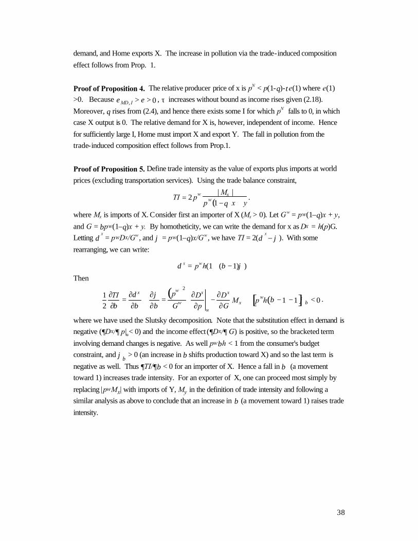
38

demand, and Home exports X. The increase in pollution via the trade-induced composition

effect follows from Prop. 1.

Proof of Proposition 4. The relative producer price of x is pN < p(1-θ)-τe(1) where e(1)

>0. Because εMD, I > ε > 0 , τ increases without bound as income rises given (2.18).

Moreover, θ rises from (2.4), and hence there exists some I for which pN falls to 0, in which

case X output is 0. The relative demand for X is, however, independent of income. Hence

for sufficiently large I, Home must import X and export Y. The fall in pollution from the

trade-induced composition effect follows from Prop.1.

Proof of Proposition 5. Define trade intensity as the value of exports plus imports at world

prices (excluding transportation services). Using the trade balance constraint,

TI = 2 pw | Mx |pw 1 −θ( )x + y

.

where Mx is imports of X. Consider first an importer of X (Mx > 0). Let Gw = pw(1–θ)x + y,

and G = βpw(1–θ)x + y. By homotheticity, we can write the demand for x as Dx = h(p)G.

Letting δ x = pwDx/Gw, and ϕ = pw(1–θ)x/Gw, we have TI = 2(δ x

– ϕ). With some

rearranging, we can write:

δ β ϕx wp h= + −( ( ) )1 1

Then

12

∂TI∂β

=∂δ x

∂β+

∂ϕ∂β

=pw( )2

Gw∂Dx

∂pu

−∂Dx

∂GM x

+ pwh β −1( )−1[ ]ϕβ < 0 .

where we have used the Slutsky decomposition. Note that the substitution effect in demand is

negative (∂Dx/∂ p|u< 0) and the income effect (∂Dx/∂ G) is positive, so the bracketed term

involving demand changes is negative. As well pwβh < 1 from the consumer's budget

constraint, and ϕβ > 0 (an increase in β shifts production toward X) and so the last term is

negative as well. Thus ∂TI/∂β < 0 for an importer of X. Hence a fall in β (a movement

toward 1) increases trade intensity. For an exporter of X, one can proceed most simply by

replacing |pwMx| with imports of Y, My in the definition of trade intensity and following a

similar analysis as above to conclude that an increase in β (a movement toward 1) raises trade

intensity.

Appendix B: Data Set Description

The dependent variable in our study is the concen-tration of sulphur dioxide at observation sites in ma-jor cities around the world as obtained through theGEMS/AIR data set supplied by the World HealthOrganization. Measurements are carried out usingcomparable methods. Each observation station re-ports annual summary statistics of SO � concentra-tions such as the median, the arithmetic and geomet-ric mean, as well as 90th and 95th percentiles.

We have chosen to use a logarithmic transforma-tion of the median SO � concentration as our depen-dent variable. The distribution of concentrations ishighly-skewed towards zero when viewed on a lin-ear scale. As was pointed out in the WHO (1984)report about the GEMS/AIR project, concentrationsare more suitably described by a log-normal distri-bution with a number of observations concentrated atthe measurement threshold of the measurement de-vices. There is also an ambient level of SO � in theair that has natural causes.

A large share of observations were from the UnitedStates due to this country’s extensive network of airquality measurement stations. Other large contribu-tor countries were China, Canada, and Japan. Manyof the other observation stations provided short ordiscontinuous streams of data while participating inthe GEMS/AIR project. All in all, our analysis isbased on over 2,600 observations from 293 obser-vation stations in 109 cities around the world; thesecities are located in 44 countries.

The primary source for our data is the AIRS Execu-tive International database that contains informationabout ambient air pollution in nations that voluntarilyprovide data to the GEMS/AIR program sponsoredby the United Nations World Health Organization.1

We had problems with the identification of severalobservation stations. The longitude and latitude in-formation provided in one of the ancillary files was insome cases incorrect and was corrected case-by-casebased on the the description of the location.

Additional data sources for our regressors includethe Penn World Tables2 for macroeconomic data,the World Investment Report3 for inward FDI stockdata, the CIESIN Global Population DistributionDatabase4 for population density data, the WorldResources Insititute World Resources Database5 fornatural resources and physical endowments, and data

from the Global Historical Climatology Network6

(GHCN) for weather conditions at the observationstations. Yet more time series were obtained for tariffand non-tariff trade barriers,7 and educational attain-ment.8

Summary statistics for the major variables appearin table B-1. Some of the variables warrant furtherexplanation. First, our scale measure of economic ac-tivity GDP per square kilometre is calculated by mul-tiplying a country’s real per-capita GDP ($/person)with each city’s population density (people/km

�).

Extrapolations for per-capita GDP were carried outfor the years past 1993 based on real growth rates ob-tained from the IMF/IFS statistics. Population densi-ties were available only for 1990.

The capital abundance (K/L) of countries was ob-tained from the physical capital stock per workervariable in the Penn World Tables. We have adjustedthis series for human capital by applying a 0–1 aver-

���This package is available from the United States Environ-

mental Protection Agency (US-EPA) at http://www.epa.gov/-airs/aexec.html. The US-EPA kindly provided a much morecomplete version of this dataset that included not only averagesbut also median and other percentiles of SO � concentrations. Wewould like to express our gratitude to Jonathan Miller of the US-EPA for providing additional GEMS/Air data not contained inthe public release of the database, and for patiently answering ournumerous technical questions.���

Robert Summers and Alan Heston, “The Penn World Ta-ble (Mark 5): An Expanded Set of International Comparisons,1950–1988”, Quarterly Journal of Economics, Vol. 106, May1991, pp. 327–368. Available in revision 5.6 from the Center forInternational Comparisons at the University of Pennsylvania athttp://pwt.econ.upenn.edu/.� �

United Nations Centre on Transnational Corporations, 1992and 1999 volumes.��

This data set from the Consortium for International EarthScience Information Network (CIESIN) is only available for1990. It can be obtained freely from the United Nations En-vironmental Programme server maintained by the U.S. Geo-logical Survey at http://grid2.cr.usgs.gov/globalpop/1-degree/-description.html. �

World Resources 1998-1999: A Guide to the Global Envi-ronment”, Oxford University Press, Oxford: 1998.��

Information is available on monthly average temperatures,monthly precipitation, and atmospheric pressure. The raw dataand description file are available from the National Climatic DataCenter of the U.S. National Oceanic and Atmospheric Adminis-tration at ftp://ftp.ncdc.noaa.gov/pub/data/ghcn/v1/.� �

See Sachs and Warner (1995). �These figures were obtained from Robert J. Barro and Jong-

Wha Lee 1994 study, available from the NBER web site athttp://www.nber.org/pub/barro.lee/ZIP/.

40

TABLE B-1: SUMMARY STATISTICS

Variable Dimension Obs. Mean Std.Dev. Min. Max.Log of SO2 log(ppm) 2555 -2.112 0.481 -3.000 -0.939City Economic Intensity $m per km

�2555 0.790 0.878 0.010 5.934

GDP per capita (current) $10k 2555 1.478 0.862 0.109 2.718Population Density 1000p/km

�2555 0.063 0.055 0.001 0.276

Capital Abundance (adjusted) $10k/worker 2555 5.612 2.497 0.829 17.189Capital Abundance (unadjusted) $10k/worker 2555 3.207 1.763 0.130 7.750Education Attainment 0-1 range 2555 0.540 0.226 0.088 0.799GNP per capita, 3yr avg. $10k 2555 1.396 0.815 0.111 2.635Communist Country [—] 2555 0.125 0.331 0.000 1.000C.C. � Income $10k 319 0.302 0.208 0.127 0.716Trade Intensity (X+M)/GDP [—] 2555 0.409 0.322 0.088 2.617Relative

���������(adj.) World=1.00 2555 1.357 0.605 0.203 4.174

Relative Income World=1.00 2555 2.500 1.392 0.221 4.138Inward FDI Stock / Capital Stock [—] 2525 0.106 0.250 0.001 2.193Avg. Temperature � C 2555 14.689 5.600 2.617 28.967Precipitation Coeff. of Var. [—] 2555 0.011 0.006 0.001 0.054Hard Coal Reserves GJoule/worker 2555 0.040 0.043 0.000 0.146Soft Coal Reserves GJoule/worker 2555 0.038 0.052 0.000 0.348

Note: All monetary figures are in 1995 US Dollars. The interaction term for income with the communist countries dummy onlyshows the case where the the dummy is equal to one; thus the mean for this line is the mean for the communist countries only.

age education index (in which 1 represents 16 yearsof schooling) obtained from the Barro/Lee data set.Relative capital abundance is obtained by dividingeach country’s capital abundance by the correspond-ing world average for the given year, where “worldaverage” is defined by all the countries in the PennWorld Tables.

Our income (I) variable is the three-year averageof lagged GNP per capita. This addresses two prob-lems. First, contemporaneous income and the level ofpollution may be determined simultaneously. Laggedincome, however, is exogenous. Second, it is rea-sonable to assume that income changes translate onlyslowly into policy changes. We therefore smooth outsome of the variation introduced through business cy-cles and include three years of data. (We also experi-mented with longer lags, without much effect on ourresults.) More concretely, for a given year � we com-pute ����� �! �!"$#&% �!" � % ��"(' �)��* . Relative incomeis constructed in the same fashion as our relative cap-ital abundance measure. GNP figures were obtainedby adjusting GDP figures with a GNP/GDP correc-tion factor obtained from the International MonetaryFund’s International Financial Statistics. However,such correction factors were unavailable for the for-

mer Czechoslovakia, Egypt, Hong Kong, Iraq, Pery,Poland, and the former Yugoslavia. Unadjusted GDPfigures were used in these cases.

The data on foreign direct investment were ob-tained as percentages of the stock of inward FDI rela-tive to GDP, and interpolated where necessary. Thenthese figures were divided by GDP to capital stock ra-tios obtained from the Penn World Tables in order toobtain the percentage of inward FDI stock relative toa country’s entire capital stock.

The suburban and rural location type dummy vari-ables are from the oiriginal GEMS/AIR dataset. Thethird (default) location type is central city. Our tradeintensity measure is calculated as the sum of ex-ports and imports expressed as a percentage of grossdomestic product. The communist country dummyused in our study identifies the following countries:China, Czechoslovakia, Poland, and Yugoslavia. Thecountry dummy for the Helsinki Protocol identi-fies Austria, Belgium, Bulgaria, Canada, Czechoslo-vakia, Denmark, Finland, France, Germany, Hun-gary, Italy, Luxembourg, The Netherlands, Norway,and Switzerland, in the years after 1985.

41

39

References Antweiler, W., Copeland, B.R. and M.S. Taylor, "Is Free Trade Good for the Environment,"

National Bureau of Economic Research, WP 6707, August (1998).

Chay, K.Y. and M. Greenstone, “The Impact of Air Pollution on Infant Mortality: evidence from geographic variation in Pollution shocks induced by a Recession”, NBER working paper No. 7442, December (1999).

Copeland, B.R. and M.S. Taylor, "North-South Trade and the Environment," Quarterly Journal of Economics, 109 (1994): 755-87.

Copeland, B.R. and M.S. Taylor, "Trade and Transboundary Pollution," American Economic Review, 85 (1995): 716-737.

Dean, J.M, “Testing the Impact of Trade Liberalization on the Environment: Theory and Evidence”, mimeo, John Hopkins University (1998).

Dixit, A.K. and V. Norman, Theory of International Trade, Cambridge University Press, Cambridge (1980).

Ferrantino, M. and L. Linkins “Global Trade Liberalization and Toxic Releases”, US International Trade Commission discussion paper (1996).

Gale, L.R. and J.A. Mendez, "A note on the relationship between trade, growth, and the environment," International Review of Economics and Finance, 7 (1998): 53-61.

Grossman, Gene M, and Alan B. Krueger, “Environmental Impacts of a North American Free Trade Agreement, “ in The U.S.-Mexico Free Trade Agreement, P. Garber, ed. (Cambridge, MA: MIT Press, 1993)

Grossman, Gene M, and Alan B. Krueger, “Economic Growth and the Environment, Quarterly Journal of Economics, (1995): 353-377.

Harrigan, J. “Factor Endowments and the international location of production: Econometric Evidence for the OECD, 1970-1985”, Journal of International Economics, 39, (1995): 123-141.

Harrigan, J. “Technology, Factor supplies, and International Specialization: Estimating the

Neoclassical model”, American Economic Review , 87, (1997): 475-494. Jaffe, A., S. Peterson, P. Portney and R. Stavins, "Environmental Regulation and the

Competitiveness of U.S. Manufacturing: What Does the Evidence Tell Us?" The Journal of Economic Literature, (1995)

Kraushaar, Jack J. and Robert A. Ristinen, Energy and Problems of a Technical Society.

New York: John Wiley & Sons, (1998).

40

Levinson, A. "Environmental Regulations and Industry Location: International and Domestic Evidence", in Fair Trade and Harmonization: prerequisites for free trade, J.N. Bhagwati and R.E. Hudec ed. (Cambridge, MA: MIT Press, 1996)

Lucas, D. Wheeler, and H. Hettige. "Economic Development, Environmental regulation and the International Migration of Toxic Industrial Pollution: 1960-1988, in Low P (ed) International Trade and the Environment, World Bank discussion paper, No. 159 (1992): 67-86.

Low, P. and A. Yeates. "Do 'dirty' Industries Migrate", in Low P (ed) International Trade and the Environment, World Bank discussion paper, No. 159, (1992): 89-104.

Mani, M. and D. Wheeler. “In search of pollution havens?: dirty industry migration in the world economy," World Bank Working paper No. 16, April (1997).

McGuire, M. C. "Regulation, Factor Rewards, and International Trade", Journal of Public

Economics, 17 (1982):335-354. Pethig, R. "Pollution, Welfare, and Environmental Policy in the Theory of Comparative

Advantage", Journal of Environmental Economics and Management, Vol. 2, Feb. (1976):160-169.

Selden, T.M. and D. Song, “Environmental Quality and Development: Is there a Kuznets

Curve for Air Pollution Emissions?” Journal of Environmental Economics and Management, 27, (1994):147-162.

Shafik, Nemat “Economic Development and Environmental Quality: An econometric analysis”, Oxford Economic Papers 46 (1994):757-773.

Siebert, H., J. Eichberger, R. Gronych, and R. Pethig, Trade and the Environment: A Theoretical Enquiry (Amsterdam: Elsevier/North Holland, 1980).

Tobey, J.A., "The effects of domestic environmental policies on patterns of world trade: An empirical test," Kyklos, 43, (1990): 191-209.

United Nations Environment Programme, Urban Air Pollution. Nairobi: UNEP (1991)

Woodland, A.D. International Trade and Resource Allocation, North-Holland, Amsterdam (1982).

World Health Organization, Urban Air Pollution: 1973-1980. Published under the joint sponorship of United Nations Environment Programme and the World Health Organization. Geneva, (1984).