IPO Waves, Product Market Competition, and the Going Public Decision:

Theory and Evidence

Thomas J. Chemmanur*

and

Jie He**

Forthcoming, Journal of Financial Economics

*Professor, Finance Department, Fulton Hall 440, Carroll School of Management, Boston College, Chestnut Hill, MA 02467, Tel:

(617) 552-3980, Fax: (617) 552-0431, email: chemmanu@bc.edu.

**Assistant Professor, Department of Banking and Finance, 424 Brooks Hall, Terry College of Business, University of Georgia,

Athens, GA 30602, Tel: (706) 542-9076, Fax: (706) 542-9434, email: jiehe@uga.edu.

For helpful comments and discussions, we thank Kenneth Ahern, Pierluigi Balduzzi, Walid Busaba, David Chapman, Craig Dunbar,

Joseph Fan, Shan He, Clifford Holderness, Gang Hu, Jiekun Huang, Tim Jenkinson, Yawen Jiao, Karthik Krishnan, Praveen Kumar,

Alan Marcus, Ronald Masulis, Debarshi Nandy, Tom Noe, Neil Stoughton, Paul Povel, Jun Qian, Jonathan Reuter, Ronnie Sadka,

Philip Strahan, Robert Taggart, Hassan Tehranian, and Xuan Tian. We also thank seminar participants at Boston College, The Chinese

University of Hong Kong, Concordia Univesity, George Washington University, Hebrew University of Jerusalem, Nanyang Technological

University, National University of Singapore, Oxford University, Singapore Management University, Tel-Aviv University, University of

Georgia, University of Houston, University of Illinois at Chicago, University of New South Wales, University of Western Ontario, and

conference participants at the RICAFE 2008 conference at Amsterdam, the FIRS 2009 Meetings at Prague, the 2009 Southwestern Finance

Association Meetings, the 2009 Financial Management Association Meetings, the 2009 Midwestern Finance Association Meetings, the

2009 Eastern Finance Association Meetings, the 2009 Northern Finance Association Meetings, and the 2009 Southern Finance Association

Meetings for helpful comments. Special thanks to Bill Schwert and an anonymous referee for several helpful comments. The research

presented in this paper was conducted while the authors were special sworn status researchers at the Boston Research Data Center of

the U.S. Census Bureau. Any opinions and conclusions expressed herein are those of the authors and do not necessarily represent the

views of the U.S. Census Bureau. All results have been reviewed to ensure that no confidential information is disclosed. Any remaining

errors or omissions are the responsibility of the authors.

IPO Waves, Product Market Competition, and the Going Public Decision:

Theory and Evidence

ABSTRACT

We develop a new rationale for IPO waves based on product market considerations. Two firms, with differing

productivity levels, compete in an industry with a significant probability of a positive productivity shock. Going

public, though costly, not only allows a firm to raise external capital cheaply, but also enables it to grab market

share from its private competitors. We solve for the decision of each firm to go public versus remain private, and the

optimal timing of going public. In equilibrium, even firms with sufficient internal capital to fund their new investment

may go public, driven by the possibility of their product market competitors going public. IPO waves may arise in

equilibrium even in industries which do not experience a productivity shock. Our model predicts that firms going

public during an IPO wave will have lower productivity and post-IPO profitability but larger cash holdings than

those going public off the wave; it makes similar predictions for firms going public later versus earlier in an IPO

wave. We empirically test and find support for these predictions.

IPO Waves, Product Market Competition, and the Going Public Decision:

Theory and Evidence

1 Introduction

The existence of IPO waves, otherwise known as "hot" IPO markets, has been widely documented: see, e.g., Ritter

(1984). The reasons for the existence of such IPO waves, however, are less widely understood. Two recent theoretical

models of IPO waves are Pastor and Veronesi (2005) and Alti (2005). Pastor and Veronesi (2005) argue that IPO

waves are generated due to the "real option" effect of going public: entrepreneurs possess a real option to take their

firms public, invest part of the IPO proceeds, and begin producing, and, in a setting of time-varying market conditions,

choose the best time to exercise this option. When stock market conditions are sufficiently favorable (expected market

return is low, expected aggregate profitability is high, and prior uncertainty is high), many entrepreneurs exercise

their options to go public, thus generating an IPO wave. Alti (2005) focuses instead on information spillovers across

IPOs to generate IPO waves. He considers a setting in which IPOs are sold to institutional investors, who are

asymmetrically informed about a valuation factor common across private firms. Since IPO offer prices are set based

on investors’ indications of interest, the outcome of an IPO (a high versus low IPO offer price) reflects information

that was previously private, reducing information asymmetry across investors and reducing valuation uncertainty for

future issuers, thereby triggering an IPO wave.

While the above two theoretical analyses have driving forces quite different from each other, they also have one

feature in common: they are both driven by considerations of stock market valuation and stock returns: the aggregate

stock market in the case of Pastor and Veronesi (2005), and stock valuation in the IPO market in the case of Alti

(2005). While stock market valuation is indeed an important driving force behind the creation of IPO waves, another

driving force that has not been analyzed so far in the literature is product market competition. The objective of

this paper is to develop a theory of the timing of a firm’s going public decision and IPO waves based on product

market considerations that allow us to answer several interesting questions: First, which industries are most likely

to have an IPO wave? Second, what are the differences between firms that go public "on the wave" (i.e., as part of

an IPO wave) versus "off the wave" (i.e., either individually, or part of a cold IPO market) both in terms of pre-IPO

productivity and post-IPO product market performance? Third, within the set of firms going public as part of an

IPO wave, does timing matter: i.e., is there a difference in productivity and post-IPO performance (as well as other

firm characteristics) between firms that go public earlier in an IPO wave versus later in the wave?1 Our theoretical

1While we are not aware of any prior empirical analyses of this question, there is some anecdotal evidence that higher quality firms

go public earlier in an IPO wave: see, e.g., the Harvard Business School Case ImmuLogic Pharmaceutical Corporation (B-2). To quote:

"The one certainty about the current open window for biotechnology initial public offerings (IPOs) was that sooner or later it would

shut again. Furthermore, he (Henry McCance) has observed that in past periods of intense IPO activity, the best firms tended to go

public early in the cycle, while lower-quality firms went public later." See also Ritter and Welch (2002) for a discussion of practitioner

1

model answers these and related questions, and we empirically test the implications of our theory.

Our theory departs from existing analyses with the assumption that going public not only allows a firm to raise

capital at a lower cost than if it were a private firm, but also allows it to grab market share from competitors who

remain private. It is particularly interesting to examine, both theoretically and empirically, the implications of the

notion that going public enables a firm to grab market share from competitors in the product market, since there is

some anecdotal evidence from practitioners that this is indeed the case in practice.2 We do not make any assumptions

regarding the precise mechanisms through which firms going public early are able to grab market share from their

competitors: possible mechanisms include gaining additional credibility with customers and suppliers; being able to

hire higher quality employees as a public firm and rewarding them more efficiently using stock and stock options; and

being able to acquire related firms in the same industry (holding patents valuable for introducing various product

innovations) through takeovers paid for using their own (publicly traded) stock.3

We consider an industry with two firms: firm 1 and firm 2, both of which are private to begin with. Each firm has

a scalable project with decreasing returns to scale, which it proposes to implement. Firm 1 has higher productivity

of capital compared to firm 2, so that its equilibrium scale of investment is higher than that of firm 2. Each firm has

a certain amount of internal capital available to it as a private firm. However, if the amount of capital required for

investment exceeds the above internal capital, the firm needs to either scale back its investment (i.e. operate at a

scale smaller than its optimal level) or raise external financing by going public.4 Thus, going public has two benefits

in our setting: it allows the firm to raise external financing if necessary, and also allows it to grab market share from

other firms in the industry that are private. On the other hand, going public is costly: we assume that each firm has

to incur a significant cost if it chooses to go public.

Each firm knows its own productivity, and also that their industry may soon experience a positive productivity

shock with a certain probability. We assume that, in the absence of a productivity shock, the available internal capital

will be enough to fund the projects of both firm 1 and firm 2 at their optimal scale. If, however, a productivity

shock is realized, firm 1 (which has higher productivity to begin with) needs to go public to raise external financing

arguments on the timing of firms going public within an IPO wave.2To quote Killian, Smith, and Smith (2001): "An IPO can establish its brand and gain loyal customers ahead of competitors. Palm

established itself as the leader with a suite of spiffy handheld devices and great marketing, grabbing 80 percent of market share. Then

Handspring, founded by Palm alums, created a device with a twist: add-on modules that allow Handspring users to download and play

music or to access the Internet. Handspring priced its PDAs aggressively and captured most of the remaining (market) share. With these

two aggressive players dominating PDA sales, it was very difficult for a new entrant to compete. Even Microsoft, with its billions of dollars

of marketing clout, retreated from the field." Killian, Smith, and Smith (2001) also give a number of examples from other industries where

firms that went public earlier were able to grab significant market share in their industry. Examples include Affymetrix, the maker of

microchips that identify and analyze gene sequences; Petsmart, the pet superstore, which went public ahead of its competitor, pets.com,

and grabbed significant market share; and Capstone Turbine, the maker of microturbines, which was the first to introduce such turbines

for commercial use.3Another possibility is that a public firm may compete more aggresively in the product market than a private firm, since a risk-averse

entrepreneur may find it easier to diversify his personal portfolio and therefore care less about operating risk after going public: see Chod

and Lyandres (2010), who develop a model formalizing this argument.4Thus, for simplicity, we assume that it is prohibitively costly for the firm to raise external financing as a private firm. However, note

that all our results go through as long as the cost of external financing is significantly cheaper for a public firm compared to that for a

private firm.

2

in order to operate at its new optimal scale, while firm 2 will continue to have enough internal capital to operate at

its new optimal scale (since, given its lower level of initial productivity, its new optimal scale will be smaller than

its available internal capital even after the productivity shock is realized). We allow a firm to go public either early

(before the productivity shock is realized) or late (after the shock is realized). We assume that there will be two

rounds of competition for market share between the two firms in the product market: one before the productivity

shock is realized, and another one afterward.

We solve for the equilibrium time at which each firm goes public (if at all), which in turn determines whether

or not there is an IPO wave (we define an IPO wave as a situation where both firms in the industry go public).

There are five possible equilibria in our model, depending on the following four parameter values: the magnitude

of a potential productivity shock; the probability of a productivity shock; the cost of going public; and the levels

of initial productivity of each firm in the industry. Consider first the benchmark equilibrium, where going public

merely allows a firm to raise external financing (and does not give it any advantage in terms of competing for market

share). In this case, the lower productivity firm 2 remains private throughout, regardless of whether or not there is

a productivity shock, since going public is costly and it has adequate capital to fund its project at its optimal scale

even in the event of a productivity shock. Firm 1 will go public only if a productivity shock is realized, since going

public does not give it any advantage in terms of competition for market share, and the only reason for going public

is to raise external financing (which becomes necessary if and only if a productivity shock is realized).

Consider now the full-fledged model, where going public enables a firm to grab market share from competitors.

There are three categories of equilibria in this case, depending on the model parameters discussed earlier. The first

category of equilibria involves an IPO wave occurring even without the realization of a productivity shock: i.e., both

firms go public early without waiting to see whether a productivity shock is realized or not. The second category of

equilibria involves both firms going public, but at least one of the two firms goes public only if a productivity shock

is realized: in other words, an IPO wave occurs only in the event of a productivity shock. The third category of

equilibria involves firms going public off the wave: i.e., only one of the two firms goes public, and the other remains

private throughout.

To understand the intuition behind the above equilibria, it is useful to consider the costs and benefits of going

public versus remaining private, as well as those of going public early versus late. Consider first firm 1. This firm

has two benefits from going public. First, in the event of a productivity shock, its internal capital is not sufficient to

fund its investment to its optimal level, so that it needs to raise additional capital by going public. Second, by going

public, it can grab market share from firm 2, in the event that the latter remains private. Its cost of going public

is the deadweight cost discussed earlier. Now consider firm 2. Since its productivity is lower, its only benefit from

going public is to prevent firm 1 from grabbing market share from it (and to grab market share from firm 1 in the

event that it does not go public); recall that we have assumed that firm 2’s initial productivity is low enough that,

3

even after the shock, it can still fund its investment at its optimal level using internal capital. Note, however, that

a productivity shock nevertheless increases its benefit of going public, since its profits from additional market share

will be greater if its productivity is greater. For either firm, the trade-off between going public early versus late is

as follows. The advantage of going public early is that the firm is able to grab market share from the other firm

(and to prevent the other firm from grabbing market share from it) in two rounds of product market competition.

The disadvantage of going public early is that it incurs the cost of going public before it knows for sure whether a

productivity shock is realized (so that the firm may end up being public in a situation where no shock is realized,

and it would have been better off remaining private). Note that the benefit of going public early versus late is always

greater for firm 1 than for firm 2 (since it has multiple reasons for going public, while firm 2 has only the benefit of

grabbing market share); on the other hand, the cost of going public is the same for both firms. We show that the

above trade-offs result in the higher productivity firm going public alone in equilibrium in the absence of an IPO

wave. Further, if the equilibrium involves an IPO wave, the higher productivity firm always goes public either earlier

than or at the same time as the lower productivity firm.

Our theoretical analysis yields several testable predictions. The first prediction is that, on average, firms going

public outside an IPO wave (i.e. in a cold market) will have higher productivity and post-IPO profitability than

those going public within an IPO wave. Second, on average, firms going public earlier in an IPO wave will have

higher productivity and post-IPO profitability than those going public later in the wave. Third, since our model

predicts that firms going public outside an IPO wave have higher average pre-IPO productivity, and given that

higher-productivity firms have a larger optimal scale, firms going public in an IPO wave will on average hold more

cash on hand than firms going public off the wave (for a given amount raised in the IPO). Similarly, our model

predicts that firms going public later in an IPO wave will on average hold more cash on hand than firms going public

earlier in the wave (for a given amount raised in the IPO).

Before testing the implications of our theory, we first provide some evidence regarding our model assumption that

going public allows a firm to grab market share from competitors who remain private. For this empirical analysis, we

make use of the Longitudinal Research Database (LRD) of the U.S. Census Bureau, which covers the entire universe

of private and public U.S. manufacturing firms. We find that IPO firms experience an increase in their market share

soon after they go public at the expense of their private competitors (Table 3). Further, IPOs in a given industry are

associated with a reduction in the market share of same-industry competitors, and this negative correlation is larger

for competitors that are private (Table 4).5 There are two possible scenarios that can explain the above findings.

First, going public causes an increase in the IPO firm’s market share and a reduction in its competitors’ market share

5See also Hsu, Reed, and Rocholl (2010), who document that firms experience negative stock price reactions to completed IPOs in

their industry and positive stock price reactions to IPO withdrawals. Further, they show that following a successful IPO in their industry,

competing firms show significant deterioration in their operating performance. Slovin, Sushka, and Ferraro (1995) present similar evidence

in the context of equity carve-outs.

4

(which is our model assumption). Second, the anticipation of increased market share induces a firm to go public.

Without a valid instrument for the going public decision of a firm, it is difficult to distinguish between the above

two scenarios. Thus, while the above results are broadly consistent with the main assumption of our model, we do

not wish to claim that going public causes an increase in market share.6 In other words, the objective of the above

analysis is not to present convincing empirical support for the above assumption of our model. We believe that, like

all other models, our model should be evaluated based on the evidence we present here regarding its predictions.

We test the predictions of our model using three different data sets. We obtain our overall IPO sample from

the Thomson Financial Securities Data Corporation (SDC) new issues database. We obtain the data required to

calculate the total factor productivity (TFP) and the market share of firms remaining private as well as those going

public (or are already public) from the LRD of the U.S. Census Bureau. Finally, we obtain data on the accounting

performance of IPO firms subsequent to going public (like ROA and cash holdings) from the Compustat database.

To compare on-the-wave IPO firms versus off-the-wave ones in the same industry, we define the "hotness" of an

IPO market as the total number of IPOs in the same Fama-French industry within a 90-day window symmetrically

surrounding the issuance date for any given IPO and use this number as a raw measure of the hotness of the IPO

market in that industry for the particular issuance date under consideration. Consistent with our first prediction, we

find that a firm that goes public within a hot period of 8 other same-industry IPOs will on average have total factor

productivity (TFP) 0.028 less than a firm that goes public within a cold period of only 1 other same-industry IPO.

Given that the mean of TFP in our sample is 0.046, this represents a 61% difference in TFP, which is economically

significant. We also find that a firm that goes public within a hot period of 8 other same-industry IPOs will on average

have a post-issuance ROA 1.1% less than a firm that goes public within a cold period of only 1 other same-industry

IPO. Given that the mean of post-IPO ROA in our sample is 5%, this represents a 20% difference in post-issuance

operating performance. We also use two refinements of the above measure for hotness and find similar results.

To compare leaders and followers in an IPO wave for a particular industry, we first identify and define IPO waves

within that industry and then rank the IPOs in our sample within each wave by the order of their issuance dates.

Consistent with our second prediction, we find that a firm that goes public earlier in an IPO wave (among the first

25% of firms going public in this wave) will on average have TFP 0.081 more than a firm that goes public later in

the wave (among the last 25% of firms going public in this wave). Given that the mean of TFP in our sample is

0.046, this represents a 176% difference in TFP. Further, we find that a firm that goes public earlier in an IPO wave

(among the first 25% of firms going public in the wave) will on average have an ROA 2.3% more than a firm that

goes public later in the wave (among the last 25% of firms going public in the wave). Given that the mean ROA in

our sample is 5%, this represents a 46% difference in post-issuance ROA. Similar results hold if we use alternative

6 It is difficult to find a convincing firm-level instrumental variable for a firm’s going public decision that satisfies the exclusion

restriction requiring that the variable, while correlated with the going public decision, should not directly affect the subsequent product

market share of the firm going public.

5

measures of how early an IPO takes place within a wave.

The above empirical results regarding the TFP as well as post-IPO profitability of firms going public on the wave

versus off the wave, and that of firms going public early in a wave versus later in the wave are also consistent with

the predictions of a variation on the model of Pastor and Veronesi (2005) which relies on stock market conditions

(details in Section 7.2.1 and 7.3.1). We therefore conduct several robustness tests to distinguish our predictions from

those of that model and find that, even after incorporating proxies for short-term and long-term market conditions

as controls, there is residual empirical support for our model predictions.

We also find evidence supporting our other predictions. Our results show that, on average, firms that go public in

an IPO wave will hold more cash on hand after the IPO and experience a larger increase in cash and cash equivalents

around the IPO date than firms that go public off the wave. Similarly, we find that firms going public later in an IPO

wave on average hold a larger cash balance on hand after the IPO and experience a larger increase in cash and cash

equivalents around the IPO date than firms that go public earlier in the wave. Finally, since our model argues that

product market competition is an important factor driving firms’ going public decisions, we analyze whether and

how industry concentration relates to the relationship between post-issuance operating performance and IPO timing

("on the wave" versus "off the wave", and "early in a wave" versus "later in the wave"). We find that a higher level

of industry concentration tends to weaken the difference in post-IPO performance between firms that go public on

the wave versus off the wave, and between firms going public earlier in a wave versus later in the wave. We discuss

the implications of this finding for our theory in section 7.5.

Apart from the two theoretical analyses of IPO waves discussed earlier, the theoretical literature most directly

related to this paper is the literature on the going public decision: see, e.g., Chemmanur and Fulghieri (1999) or

Maksimovic and Pichler (2001). In a recent paper, Spiegel and Tookes (2007) develop a model of the relationship

between product market innovation, product market competition, and the public versus private financing decision

in an infinite horizon model. In their model, the advantage of going public is the ability to obtain cheaper financing

while the disadvantage is the disclosure requirements associated with going public that allow competitors in the

firm’s industry to copy the innovation. Another related model is Pastor, Taylor, and Veronesi (2009), in which an

entrepreneur trades off the diversification benefits of going public against the cost of doing so (the loss of his benefits

of control), in the presence of Bayesian learning about the average productivity of his firm. IPO waves are not the

main focus of the above models.78 In terms of empirical literature, this paper is most directly related to the papers

7Yung, Colak, and Wang (2008) develop a model in which time-varying investment opportunities lead to time-varying adverse selection

in the IPO market. They test this model taking as given the premise that asymmetric information is revealed over time, and find that

hot-market IPOs are associated with greater cross-sectional return variance and higher delisting rates. Khanna, Noe, and Sonti (2007)

develop a model of going public in which screening IPOs requires specialized labor, which is in fixed supply. A sudden increase in demand

for IPO financing increases the compensation of this screening labor, which results in reduced screening, resulting in sub-marginal firms

entering the IPO market. Their model predicts increased underpricing in hot markets. Boot, Gopalan, and Thakor (2006) study an

entrepreneur’s choice between private and public ownership when insiders and outsiders disagree about the best way to maximize firm

value.8Our paper is also broadly related to the literature on product and financial market interactions: see, e.g., Chemmanur and Yan

6

studying hot and cold IPO markets (see, e.g., Helwege and Liang 2004) and the literature studying fluctuations in

IPO volume (see, e.g., Lowry 2003, Lowry and Schwert 2002, or Benveniste, Ljungqvist, Wilhelm, and Yu 2003).

Unlike our paper, Helwege and Liang (2004) mostly study IPO waves in the entire equity market rather than with

respect to each industry, and conclude that there is no difference in the quality of firms going public in hot and

cold IPO markets. In contrast to their findings, our empirical analysis indicates that there is indeed a significant

difference in both pre-IPO productivity and post-IPO operating performance (both in the short and the long run)

between firms going public during an IPO wave versus those going public off the wave. The empirical literature on

the going public decision (see, e.g., Pagano, Panetta, and Zingales 1998 or Chemmanur, He, and Nandy 2010) is also

indirectly related to this paper.9

The rest of the paper is organized as follows. In section 2, we describe our model setup, and in section 3 we

characterize its equilibria. We describe our testable predictions in section 4 and our data and sample selection

procedures in section 5. We discuss variable construction and summary statistics in section 6. In section 7, we

describe our empirical results and conclude in section 8.

2 The Model

We consider the going public decision of two competing private firms in an industry. For simplicity, we assume that

the two firms are duopolies who split the total product market between them. The model has four dates (time 0, 1,

2, and 3). At time 0, the two private firms are endowed with the same amount of initial capital and the same form

of cash-flow-generating technology. Firm 1 has a market share of and firm 2 has the rest (1−).10 Without loss

of generality, we assume firm 1 to have a higher productivity 1 than firm 2, with productivity 2 (1 2). As

we shall see in section 2.1, both firms’ long-term (time 3) valuation increases with their market share and production

efficiency (which depends on their productivity as well as their available capital).

At time 1, each firm knows that a productivity shock may take place at time 2, in which case its productivity may

increase by amount ∆ ( 0) with probability . We denote the enhanced productivity of firm as ≡ +∆.

Given this distribution of potential shocks, the firms will calculate their expected optimal capital level and may go

public in case of an expected funding shortage. Going public, at a fixed cost of , has two benefits. First, it can

provide cheaper capital for a firm’s production than debt or private placements (i.e., we assume that alternative

financing methods are too costly to be feasible). Second, it can improve a firm’s efficiency in grabbing market share

(2008), who analyze the relationship between product market advertising and new equity issues (IPOs and SEOs), and Stoughton, Wong,

and Zechner (2001), who argue that the decision of a firm to go public may serve to signal high quality to the product market.9Our paper is also broadly related to the large theoretical and empirical literature on IPOs: see, e.g., Chemmanur (1993), Allen and

Faulhaber (1989), Welch (1989), and Grinblatt and Hwang (1989), for theoretical IPO models, and Ritter and Welch (2002) for a review.10 Since firms already gone public play no role in our model, we simply assume that they own zero market share. As a result, the sum

of market share for the two private firms is assumed to be 1. Alternatively, we can specify the sum of market share to be (0 1),

which allows our subsequent analysis to go through unaffected.

7

from its competitors, for example, by enhancing its credibility with customers and suppliers; allowing it to hire higher

quality employees as a public firm and rewarding them more efficiently using stock and stock options; or allowing it

to acquire related firms in the same industry through takeovers paid for using their publicly traded stock. After the

firms make their going public decisions, they will start the first round of product market competition, the details of

which will be discussed in section 2.2.

At time 2, productivity shocks, if any, are realized, and a firm can go public at this stage if it hasn’t already done

so at time 1. The capital raised at this stage and the enhancement in its market-share-grabbing ability will also help

the firm increase long-term (time 3) cash flows and thus raise its market valuation. The second round of product

market competition now takes place and the total market share is redivided between the two rivals.

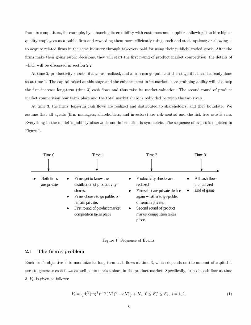
At time 3, the firms’ long-run cash flows are realized and distributed to shareholders, and they liquidate. We

assume that all agents (firm managers, shareholders, and investors) are risk-neutral and the risk free rate is zero.

Everything in the model is publicly observable and information is symmetric. The sequence of events is depicted in

Figure 1.

Time 1 Time 3

Firms get to know the

distribution of productivity

shocks. Firms choose to go public or

remain private. First round of product market

competition takes place

Time 2

Productivity shocks are

realized

Firms that are private decide again whether to go public

or remain private. Second round of product

market competition takes place

All cash flows

are realized End of game

Time 0

Both firms

are private

Figure 1: Sequence of Events

2.1 The firm’s problem

Each firm’s objective is to maximize its long-term cash flows at time 3, which depends on the amount of capital it

uses to generate cash flows as well as its market share in the product market. Specifically, firm ’s cash flow at time

3, , is given as follows:

=© (

)

1−(∗ ) − ∗

ª+ 0 ≤ ∗ ≤ = 1 2 (1)

8

where is the amount of capital firm possesses at the end of time 2. If the firm remains private for the two periods,

then is simply 0, its original capital endowment (which is assumed to be the same for both firms). If, on the

other hand, firm goes public in any period (time 1 or 2), will become 0+, where denotes the amount of

capital raised in the offering. is firm ’s market share at the end of time 2 (i.e., after two rounds of product market

competition), whose level depends on both firms’ going public decisions. The details of product market competition

are provided in section 2.2. is firm ’s productivity at time 2. If it experiences the productivity shock at time 2,

then is . Otherwise

remains at

∗ , the capital firm uses to generate cash flows, cannot exceed ,

the total amount of capital it owns at time 2. is the constant marginal cost of deploying each unit of capital (i.e.,

it is the production cost per unit of capital), 0 ≤ 1. Lastly, we adopt a Cobb-Douglas production function andassume that 0 1 so that the cash-flow generating technology exhibits decreasing returns to scale in its capital

usage.11 All parameters are publicly known.

Given the above setup, it is straightforward to show that the efficient level of capital chosen by firm , , is linearly

increasing in its long-term market share and also increasing in the firm’s productivity: ≡

( )

11− ()

1−1

and ∗ = [ ].

2.2 Product market competition

Product market competition in this model involves the firms’ campaign to gain market share by attracting each

other’s customers.12 There are two successive rounds of competition in our model, during which each firm relies on

its own market power to launch marketing campaigns and to attract customers away from its rival. Specifically, the

evolution of market share for firm is given by:

+1 =

+ (1−)

+1 −

+1 6= and = 0 1 (2)

where is firm ’s market share at the end of time and +1 is its ability to grab rivals’ market share during

the round of competition at time + 1 ( = 0 1). Here, 01 = and 0

2 = 1 −. +1 denotes the effectiveness

of marketing efforts made by firm at time + 1. While firm can grab its competitor’s time-t market share

( ≡ 1−

) with intensity +1 , the other firm (firm ) can also attract customers away from firm at the same

time. Thus its final market share depends on both players’ relative marketing abilities.

To make the model realistic yet tractable, we assume that a public firm’s ability to grab market share after its

11We assume a Cobb-Douglas type of production function to capture the idea that capital and market share are substitutes: the firm

can increase profits either by selling more (if it has greater market share) or by producing more cheaply (which involves greater investment

in capital). We adopt the above production function for analytical simplicity: adopting more complex production functions complicates

our analysis considerably without changing our results qualitatively.12The market share competition is a variant of the Lanchester (1916) battle model, which has been widely adopted in the marketing

literature. Some recent finance papers such as Spiegel and Tookes (2006) also make use of this model to characterize product market

competition.

9

IPO is linear in its existing market share. Moreover, a private firm’s ability to grab market share from competitors

is normalized to be zero. Specifically, we assume:

+1 =

½

, if firm is public

0, if firm is private 0 1 (3)

Here, denotes the per-unit-market-share advantage that a public firm enjoys relative to a private firm in terms of

product market competition. If firm goes public early (i.e. before the first round of competition at time 1), it can

grab market share from firm for two rounds (at time 1 and 2). In other words, a late IPO may be costly due to

the loss in market share at time 1.13

If a firm wants to go public, it is better off doing so at time 1 rather than delaying it to time 2: in other words,

there is a first-mover advantage from going public early. Let’s use firm 1 as an illustration. If the final industry

outcome is that both firms go public, then for firm 1, an IPO at time 1 weakly dominates an IPO at time 2. This is

due to the fact that going public at time 1 will give it an immediate competitive edge while deferring the IPO will

result in a loss of this opportunity and may even subject the firm to more aggressive competition from the rival firm.

Likewise, if the final industry outcome is that only firm 1 goes public, an IPO at time 1 is still weakly dominant. This

means that the IPO decision at time 1 is a real option driven by both capital concerns and competitive forces. While

deferring the IPO decision may save the firm the cost of going public if its productivity turns out not to increase and

it is unnecessary for it to raise external financing, doing so may sacrifice the opportunity to enlarge its market share

at an earlier date. As we will discuss in the next section, this trade-off prompts many firms to go public purely out

of product market competition concerns and drives industry-wide IPO waves.

3 Equilibrium

The equilibrium concept we use is Perfect Bayesian Equilibrium (PBE). At time 1, both firms choose to either go

public or remain private. If they go public at time 1, they have no choice to make at time 2.14 Otherwise they can

choose to go public at time 2 after observing the realization of the potential productivity shock. Therefore a PBE is

13The market-share grabbing technology that we postulate here does not allow a firm that goes public later (at time 2) to grab back

some of the market share it lost to its public competitor in the previous period (when it was private). However, even if we allow the

firm that goes public later to grab back some of the market share it lost to its competitor who went public early, our results will remain

qualitatively unchanged as long as the firm going public earlier retains some of the "first-mover advantage" it gained by going public

earlier even after its competitor goes public. As we illustrated through various anecdotes in the introduction (and document later in

our empirical analysis), this seems to be consistent with practice, at least in many industries. Further, a large theoretical literature in

industrial organization has demonstrated that first movers can obtain significant permanent advantages in the product market through a

variety of mechanisms, three of which are leadership in product and process technology (e.g., Spence (1981)), preemption of scarce assets

(e.g., Schmalensee (1978)), and development of buyer switching costs (e.g., Wernerfelt (1985)): see Lieberman and Montgomery (1988)

for a review of this theoretical literature. Finally, a large empirical literature in industrial organization has documented that market

pioneers can indeed develop first-mover advantages that span decades: see Robinson, Kalyanaram, and Urban (1994) for a review of this

empirical literature.14We do not allow firms to go private once they have gone public. However, there will be no change in the equilibrium of our model

even if we relax this assumption, since, once a firm has already incurred the cost of going public, it does not have any advantage from

reverting back to become a private firm.

10

a complete characterization of all contingent strategies of the two firms in the two periods. First, we will analyze the

benchmark case where an IPO does not affect product market competition. We will then proceed to solve the full

model where an IPO enhances a firm’s competitiveness in the product market. Due to space considerations, in this

section we confine ourselves to intuitive discussions of various equilibria and the situations where they arise. Formal

propositions with proofs can be obtained from the Internet Appendix B available on the authors’ websites or from

the working paper version of this article.

3.1 Benchmark case: IPO does not affect product market competition

Given the level of newly raised capital, , and the rational expectation of the firm’s long-run market value, (),

the sharing rule between existing owners (insiders) and new shareholders during an IPO is determined as follows:

the investors will acquire () fraction of the firm and the remaining shares belong to the existing owners.

Thus, firm insiders will try to maximize the entire firm’s market value (since their stake in the firm is ()− )

and will choose its optimal investment policy. We thus do not model any agency problems between insiders and

outsiders. Insiders can choose to use only a fraction of the capital raised for investment in the firm. Further, unlike

physical production which exhausts raw materials and other inputs, the capital used here is nonperishable.15 The

firm will not use capital beyond the efficient level ( ), which in turn depends on its market share as well as its

productivity at time 2. Depending on whether firm experiences the productivity shock at time 2, can be

either (

)

11−

³

´ 1−1 ≡

(without a productivity shock) or (

)

11−

³

´ 1−1 ≡

(with a

productivity shock), where and denote firm ’s efficient level of capital per unit of market share without

and with the productivity shock, respectively. For simplicity, we assume that 1 = 2 ≡ ( −0 0), ∀ = 1 2. In other words, we assume that if either firm decides to go public, the amount raised is the same, and is large

enough to meet the investment requirement of the higher productivity firm after a productivity shock.16 Since the

investor’s participation constraint has to be satisfied, the fraction of equity sold to new investors is (). Once

15This assumption is innocuous. As long as the capital depreciation rate is the same for both firms, all our results are unaffected.16The assumption that both high and low productivity firms raise the same amount of money in their IPOs can be endogenized in an

asymmetric information setting where the precise productivity of firms (high versus low) is unobservable to outsiders, there are significant

costs associated with making additional equity issues after the IPO, and the objective of firm insiders is to maximize the long-run value

of their equity holdings in the firm. In such a setting, the market valuation of the equity of the two firms will be done in a pooling

equilibrium, where the low productivity firm mimics the high productivity firm (otherwise the low productivity firm will reveal its type

to outsiders and get a lower valuation). The high productivity firm will raise the amount of money needed for it to meet its investment

requirements in the event of a productivity shock in full (it will not raise an amount smaller than that, since it will have to incur additional

costs to make subsequent equity issues); neither will it raise a larger amount, since it wants to minimize the dilution in insider’s equity

holdings at the time of the IPO (recall that it will be undervalued in the pooling equilibrium). In such a scenario, both types of firms

would raise the same amount of money in the IPO. See, e.g., Chemmanur (1993) for an IPO model with asymmetric information where

higher and lower productivity (intrinsic value) firms raise the same amount of money in equilibrium. Since we adopt a reduced-form

modeling approach here, we have chosen not to endogeneize the IPO amount raised by introducing asymmetric information into our

setting, since this will add considerable complexity to our analysis. There is also some empirical support for the assumption that the

amount raised in a firm’s IPO is not directly related to its productivity. In an unreported empirical analysis, we find that the amount

of money raised in the IPO by higher productivity firms (measured by total factor productivity or three-year average sales growth) does

not significantly differ from that raised by lower productivity firms, after controling for firm size and stock market conditions. Moreover,

we also find empirically that the amount of money raised in the IPO is not significantly different for firms going public within a wave

versus outside a wave, and for firms going public early in a wave versus later in the wave.

11

the firm goes public, the long-run (time 3) value of firm , , is given by© (

)

1−( ) −

ª+0+−.

Without product market concerns, a firm will go public if and only if its initial capital level (0) is lower than its

efficient level ( ) and the efficiency gain from raising new capital exceeds the cost of going public . By examining

the expression for efficient capital level, we have 0 ⇔

³

1−0

´¡(

)1−¢ ≡ . Recall that

firm 1 is assumed to have higher productivity. Without loss of generality, we further assume that the productivity

shock raises firm 1’s productivity above the threshold level (1) but not that of firm 2 (2). We make the following

parametric assumption regarding the productivity levels of firms 1 and 2 with and without a productivity shock:17

⎧⎪⎪⎪⎪⎨⎪⎪⎪⎪⎩2 1

1−0

2

1−0

2

1

1−0

[−(1−)]1−≥ 1

(4)

Given the above assumption, both firms are able to operate at their optimal scale if they do not experience a

productivity shock, whether or not they go public. Likewise, firm 2 will always be able to use its efficient level

of capital whether or not its productivity increases. However, firm 1 will need new capital after experiencing a

productivity shock if it is to operate at its efficient scale, though it may also choose to remain private (and operate

at an inefficient scale) if the cost of going public is too large. Lastly, to make the model interesting, we also assume

that the cost of going public is not too large so that firm 1, upon the realization of the productivity shock, will

choose to go public even if doing so results in no additional market share.18

In the above setting, where going public does not enhance a firm’s market-share-grabbing ability (i.e. = 0 for

both public and private firms), neither firm goes public in equilibrium without a productivity shock. Further, even

with a productivity shcok, the lower productivity firm 2 will never go public. Finally, the higher productivity firm

1 will go public if (and only if) there is a productivity shock, driven only by the need to raise additional external

financing. The benchmark case thus predicts no IPO waves (or hot-issuing periods) in the absence of product market

competition (we define an IPO wave in our model to be the situation where both firms go public either at time 1 or

time 2, so that by the end of the game both are public).

17Note that this assumption is not as restrictive as it appears. The crucial assumption here is that firm 1 has higher productivity ex

ante than firm 2. The assumption that firm 1 needs new capital after the productivity shock whereas firm 2 does not (even after the

productivity shock) can be relaxed without affecting the central intuition of the paper, although such relaxation may lead to uninteresting

equilibria where both firms always want to go public at time 1 or to remain private during both periods.18This assumption is not unduly restrictive, since it simply requires that, if external financing is required, then the cash flow benefits

to firm 1 of raising such external financing by going public dominates the cost of doing so, even in absence of any product market benefits

from going public.

12

3.2 Full Model: IPO enhances product market competitiveness

In this section, we assume that going public not only provides necessary funding to firms, but also enhances their

competitiveness in the product market. Without a productivity shock, a firm’s benefit from going public purely

comes from an IPO’s enhancement in its competitiveness in the product market. We assume that the fixed cost of

going public, , exceeds these additional benefits from going public in the absence of a productivity shock. Thus,

both firms will optimally choose to remain private without a productivity shock.19

At time 1, the two firms, under the common belief that a productivity shock may take place in the future with

probability 0, consider their going public decision. We assume that the productivity shocks are industry-wide

(perfectly correlated), which means that with probability , both firm 1 and firm 2 will experience an increase in

productivity at time 2 and with probability 1− they will not.20

Unlike in the benchmark setting, in this full fledged model firm 1 has two incentives to go public: in addition

to the benefit of raising capital that it needs to operate at its optimal scale in the event of a productivity shock,

going public now has the additional benefit of increasing firm 1’s ability to grab market share from its competitor.

Knowing that firm 1 may go public, firm 2 may also wish to go public (even though it does not need to raise any

additional capital if a productivity shock is realized), since staying private will put it in a much worse product market

position. This strategic concern of firm 2 gives firm 1 an additional incentive to go public even at time 1 when the

actual productivity shock is not realized. Of course, to obtain the above benefits from going public, either firm has

to incur the deadweight cost of going public. For either firm, the trade-off between going public early (at time 1)

versus late (at time 2) is as follows. The advantage of going public early is that the firm is able to grab market

share from the competing firm (and to prevent the other firm from grabbing market share from it) in two rounds of

product market competition. The disadvantage of going public early is that it incurs the cost of going public before

it knows for sure whether a productivity shock is realized (so that the firm may end up being public in a situation

where no shock is realized, and it would have been better off remaining private). The benefit of going public early

versus late is always greater for firm 1 than for firm 2 (since it has multiple reasons for going public, while firm 2 has

only the benefit of grabbing market share); on the other hand, the cost of going public is the same for both firms.

Therefore, with product market competition, both firms may go public around the possible arrival of a productivity

shock, potentially creating an IPO wave that would not happen in the benchmark case. Depending on whether or

not an IPO wave is generated (i.e., both firms go public) and the timing of their going public, there are five possible

equilibria, which we discuss in detail in the next section.

19This assumption is not crucial for the intuition behind our results to go through, but is made only for analytical tractability.20We have also analyzed the scenario where either firm’s productivity shock is purely idiosyncratic. Most of our results remain

qualitatively unchanged even in this case. These results are available from the authors upon request.

13

3.2.1 Description of Equilibria and Intuition

There are a total of five possible Perfect Bayesian Equilibria (PBEs) in this game, which are summarized in Figure

2:21

Figure 2: Distribution of Possible Equilibria over Different Parameter Ranges

Eq1 refers to the PBE where IPO waves occur even without a productivity shock. When the magnitude of the

shock is moderate (1 − 2 ∆ ≤ ∆), the probability of the shock is large, the cost of going public is small,

and the existing productivity levels of firm 1 and firm 2 are high, both firms will go public before the realization of a

productivity shock (at time 1). The intuition here is straightforward: when both firms’ existing productivity levels

are high (close to the threshold level ), a highly probable industry-wide shock with a moderate magnitude is very

likely to render the firms’ current production scales inefficient, making firm 1 eager to obtain fresh capital through

an IPO. Since the productivity shock is likely and both firms are close to their efficient operating scales, firm 2 knows

for sure that firm 1 will go public by the end of the game (by conducting its IPO at time 1 or 2), which means

that if it does not go public, it will lose market share at least in the second round of product market competition.

The benefit of additional market share depends on the magnitude of each firm’s productivity level. Hence, the high

existing productivity level of firm 2 makes it care much about the potential loss of market share due to firm 1’s

strengthening competitive position after the IPO. When this potential loss exceeds the cost of going public, firm 2

will go public. Inferring this, firm 1’s incentive to go public is also enhanced. The cost to firm 1 from going public

at time 1 is that it wants to avoid paying an "unnecessary" cost of going public should the shock not be realized at

time 2. Therefore, when the cost of going public is considerably smaller than the expected gain in profits (due to

its high existing productivity) and given its conjecture about firm 2’s aggressive going-public strategy, firm 1 will be

21Note: the definitions of ∆ and ∆ are given in the Internet Appendix B available on the authors’ websites or from the working

paper version of this article.

14

prompted to go public at time 1 itself, even without the realization of a productivity shock. Knowing this, firm 2

will also go public at time 1 to combat firm 1 in the product market as early as possible. Consequently, both firms

end up going public at time 1, creating an IPO wave even before the realization of the productivity shock.

Eq2 and Eq3 refer to PBEs where IPO waves occur only after a productivity shock. When the magnitude of a

potential shock is large (∆ ∆), in addition to Eq1, we have two more equilibria. When the existing market

share of firm 1 is moderately large ( ≥ (2 + −√2 + 4)(2)), and the existing productivity levels of firm 1 and

firm 2 are low, both firms will remain private before the realization of a productivity shock (at time 1) and go public

only upon the realization of a shock (at time 2). This is Eq2. When the existing market share of firm 1 is small

( (2 + −√2 + 4)(2)), the existing productivity of firm 1 is high, and the existing productivity of firm 2 is

low, firm 1 will go public before the realization of a productivity shock (at time 1) and firm 2 will go public only

upon the realization of a shock (at time 2). This is Eq3.

If the existing market share of firm 1 is small enough ( (2 + −√2 + 4)(2)), Eq2, rather than Eq3, willoccur when the other parametric conditions specified above are met. The intuition is as follows. The additional

market share each firm can gain by product market competition depends on two things: the available market share

to grab from rivals (i.e. rivals’ existing market share), and its own market-share-grabbing ability, which in turn

depends on its own existing market share. When firm 1’s existing market share is much smaller than that of firm 2,

the latter’s gain in market share by going public at time 2 would be larger if firm 1 goes public at time 1 compared

to the case where firm 1 goes public only upon the realization of the productivity shock (at time 2). The reason is

that when firm 1 is currently a small player in the product market, firm 2, despite its strong market-share-grabbing

ability, has little to grab by going public, so that its gain from an IPO is small. On the other hand, when firm 1

goes public at time 1, its market share will increase in the first round of product market competition, which in turn

increases firm 2’s incentive to compete for market share in the second round of competition. Thus, firm 2’s incentive

to go public at time 2 will be stronger if firm 1 goes public at time 1 than if firm 1 delays its IPO decision. When

firm 1’s existing market share is larger than (2 + −√2 + 4)(2) and the magnitude of a potential shock ∆ is

between ∆ and ∆ , the benefit of firm 2’s going public upon a productivity shock dominates its cost of going

public if firm 1 remains private at time 1, but is less than its cost of going public if firm 1 chooses to go public one

period earlier. Thus Eq2 cannot occur whereas Eq3 can. When the magnitude of the productivity shock is very large

(∆ ∆), both Eq2 and Eq3 will exist since the initial market share distribution between the two firms does

not matter in determining the equilibrium.

Apart from the existing market share distribution, the difference in the two firms’ existing productivity levels also

determines which PBE will occur when the magnitude of the shock is at least ∆. Note that in both Eq2 and Eq3,

the existing productivity of firm 2 is so low that it has no desire to go public before a productivity shock is realized.

When the existing productivity of firm 1 is high, it has a strong incentive to go public earlier (i.e. at time 1) because

15

each unit of additional market share gained through more effective product market competition will bring it larger

time 3 cash flows. This leads to Eq3, the most interesting "sequential IPO wave equilibrium". On the other hand, if

the existing productivity level of firm 1 is also low (as that of firm 2), it will also choose to wait until the realization

of a productivity shock because the marginal benefit of additional market share gained by going public earlier does

not outweigh the cost of going public. In this scenario, we will observe Eq2, where both firms adopt exactly the same

strategy: remain private at time 1 and go public if and only if the productivity shock occurs at time 2.

Eq4 and Eq5 refer to the PBEs where IPOs only occur off the wave. When the magnitude of a potential

productivity shock is not too large (∆ ∆), we have these two equilibria in addition to the above three

PBEs. When the probability of a potential shock is low, the existing market share of firm 1 is small ( (2 + −√2 + 4)(2)), the existing productivity of firm 1 is low, and the cost of going public is large, firm 1 will go public

only upon the realization of a shock (at time 2) and firm 2 will remain private throughout. This is Eq4. When

the probability of a potential productivity shock is high, the existing market share of firm 1 is moderately large

( ≥ (2 + −√2 + 4)(2)), the existing productivity of firm 1 is high, and the cost of going public is small, firm

1 will go public before the realization of a productivity shock (at time 1) and firm 2 will remain private throughout.

This is Eq5.

In both Eq4 and Eq5, firm 2 will remain private throughout the two periods because its marginal cash flow

benefit from additional market share gained by going public is too small compared to the cost of going public. Even

though a productivity shock may improve its productivity at time 2, firm 2’s incentive to go public is still small

as the shock is not large enough to make it go public after taking into account the cost involved. Hence, the only

difference between Eq4 and Eq5 is the timing of firm 1’s going public. Eq4 will exist if the cost of going public is

very large, and when the existing productivity level of firm 1 is low. Eq5 will exist when the cost of going public

is not too large and the existing productivity level of firm 1 is high. In this case, firm 1 has a stronger incentive to

go public earlier and grab market share from firm 2. Similar to the case of Eq2 and Eq3, the existing market share

distribution affects the occurrence of Eq4 versus Eq5 when ∆ ∆ ∆ .

It is useful to understand why the probability of a potential productivity shock, , influences the occurrence of

various equilibria. Its effect on Eq1 is clear: if is larger, both firms will be more likely to go public at time 1. This is

because given the rival firm going public at time 1, there is no uncertainty with respect to the rival’s strategy at time

2, so each firm’s benefit of going public earlier (at time 1) purely depends on the probability of getting a productivity

shock. Even firm 2’s incentive to go public increases with , since the shock is large enough to make the additional

market share gained from going public early profit-enhancing. The effect of on the occurrence of Eq4 and Eq5 is

also clear: when is larger, firm 1 will be more likely to benefit from the additional market share grabbed from firm

2 if it goes public at time 1. Firm 2 will remain private throughout in both these equilibria (because its benefit of

going public is too small compared to the cost of going public), so that firm 1 does not have to be concerned about

16

the possible loss of market share due to firm 2’s going public at time 2. Thus, its incentive to go public at time 1

monotonically increases with . When is large, we are more likely to observe Eq4, whereas a small leads to Eq5.22

4 Implications and Testable Hypotheses

By inspecting the five possible PBEs above, we can see that an IPO wave (defined as both firms going public, either at

time 1 or time 2) can result from Eq1, Eq2, and Eq3, and that stand-alone IPOs can happen in Eq3, Eq4, and Eq5.23

Under all circumstances, the lower-productivity firm (firm 2 here) never goes public alone, but rather conducts its

IPO either following or at the same time as its higher-productivity rival (firm 1). This leads to the implication that

in general, stand-alone IPOs are conducted only by higher-productivity firms, but IPOs in an IPO wave involve both

high and low productivity firms. The intuition here is simple: besides product market concerns, higher productivity

firms need more capital to approach their efficient operating scales. They therefore have much stronger incentives

to go public than lower-productivity firms who merely go public under pressure from product market competition.

Hence, higher-productivity firms will go public even when doing so does not bring any additional market share. The

same intuition also leads to the implication that everything else equal, firms going public in an IPO wave will, on

average, have lower post-IPO operating performance than firms going public off the wave. This is because if two

firms in an industry having an identical initial capital level (0) raise the same amount of equity () and have

the same post-IPO market share ( ), then the higher productivity firm will also have better post-IPO operating

performance. In summary, our model predicts that, on average, firms going public outside an IPO wave (i.e. in

a cold market) will have higher productivity (H3) and better post-IPO profitability (H5) than those going public

within an IPO wave.

We do not have an equilibrium in which firm 2 goes public at time 1 and firm 1 follows suit at time 2 (thus

creating a "sequential IPO wave"). In fact, as we have discussed in the last section, firm 2 will never go public alone

at time 1. Eq3 is the only equilibrium that may generate an IPO wave that spans both time 1 and 2, given that an

industry-wide productivity shock actually takes place. The intuition why firms with superior pre-IPO productivity

are more eager to go public early on in a given wave is as follows. Both types of firms need to evaluate the benefits

and costs of waiting to go public. On the one hand, the cost of waiting, which is the loss of the opportunity to

gain market share, is larger for the higher-productivity firm 1, due to its superior cash-flow generating ability per

unit of market share. On the other hand, the benefit of waiting until time 2, which arises from being able to avoid

22The effect of on the occurrence of Eq2 and Eq3, however, is ambiguous. For these two equilibria to be possible, the magnitude

of the shock must be large enough so that firm 2, in addition to firm 1, will also find it desirable to go public at time 2 if the shock is

realized. The difference between the two equilibria is firm 1’s choice of IPO timing. On the one hand, a higher gives firm 1 stronger

incentives to go public at time 1 because it knows there is a bigger chance that it will need additional capital after the shock occurs. This

concern tends to make Eq3 more likely than Eq2. On the other hand, a higher means that firm 2 is also more likely to go public at

time 2 when the shock is realized, reducing the additional market share that firm 1 expects to grab by going public before the shock is

actually realized (at time 1). Given this, firm 1 may wish to delay its IPO decision until time 2, leading to Eq2.23Eq3 may involve an IPO wave (if a productivity shock is realized) or only one firm (firm 1) going public (if the shock is not realized).

17

incurring the cost of going public unnecessarily if the productivity shock does not take place, is larger for firm 2

(the lower-productivity firm), since its only benefit of going public comes from considerations of product market

competition (recall that firm 2 does not need additional capital to operate at its optimal scale). Whether or not

the productivity shock occurs, firm 2 does not need extra capital for production, so that if it goes public at time

1, it pays the cost of going public only for product market reasons. In summary, the expected cost of going public

"unnecessarily", arising from the scenario where the firm goes public early (at time 1) but a productivity shock is not

realized at time 2, is bigger for firm 2, which implies that the benefit of waiting is also larger for lower-productivity

firms. Comparing both the costs and benefits of waiting for the two types of firms will give rise to the prediction

that firms with higher pre-IPO productivity will go public earlier within an IPO wave. This fact also means that

these (higher productivity) firms that go public earlier in an IPO wave will perform better after the IPO than those

that go public later in the wave, if they have the same level of post-IPO capital stock and market share. Thus, our

model predicts that everything else equal, a firm that goes public earlier in an IPO wave will have higher post-IPO

operating performance on average than a firm that goes public later in the wave. In summary, our model predicts

that, on average, firms going public earlier in an IPO wave will have higher productivity (H4) and better post-IPO

profitability (H6) than those going public later in the wave.

Since higher-productivity firms in general need more capital for expansion, our next hypothesis (H7) is that

controlling for the total amount of proceeds raised, firms going public in an IPO wave will on average hold more cash

on hand (or use less of the amount raised through their IPO) than firms going public off the wave. Similarly, we have

the hypothesis (H8) that controlling for the total amount of proceeds raised, firms going public earlier in an IPO

wave will on average hold less cash on hand (or use more of the cash raised through their offerings for investment)

than firms going public later in the wave. The above two predictions arise from our assumption that both high and

low productivity firms raise the same amount of money in the IPO. Since higher productivity firms have a larger

optimal scale (investment requirement) than lower productivity firms, they are left with less cash after investing

in their projects than lower productivity firms. As we discuss in section 3 (footnote 16), this assumption can be

endogenized in a setting of asymmetric information where only firm insiders can observe the true productivity of a

firm and there are significant transaction costs to making additional equity issues after the IPO.24

The predictions of our model regarding the effect of industry concentration on the pre-IPO productivity and

post-IPO profitability of firms going public on the wave versus off the wave and earlier in the wave versus later in

the wave are ambiguous. On the one hand, for an industry characterized by a few large players (high concentration),

24Note also that the above two predictions can be generated even in the absence of the assumption that the IPO amount raised by the

two kinds of firms are the same, as long as the IPO amount raised by both firms is greater than their optimal investment requirement, and

this difference between the IPO amount raised and the optimal investment requirement is proportionately greater for low productivity

firms than for high productivity firms. The latter condition is likely to hold as long as there are significant economies of scale in raising

external financing in an IPO, which seems to be the case in practice: see, e.g., Ritter (1987), who documents that the cost of going public

is significantly larger (as a proportion of the IPO amount raised) when the IPO issue amount is smaller.

18

any competitor’s IPO will exert a large product market pressure on the rest of the firms in the industry, which may

then go public, thereby creating an IPO wave. This leads to the prediction that greater industry concentration will

amplify the difference in post-IPO operating performance for firms going public on the wave versus those going public

off the wave, and between those going public earlier in a wave versus those going public later in the wave. On the

other hand, it may be the case that larger firms that already have significant market share in an industry as private

firms do not have too much to gain by going public. This is because such firms already have considerable credibility

with potential employees, customers, and suppliers even as private firms. In this case, firms in more concentrated

industries will be less likely to go public out of product market concerns, attenuating the above difference. In sum,

the effect of industry concentration on the difference in post-IPO operating performance for firms going public on

the wave versus off the wave and earlier in a wave versus later in the wave is an empirical question, and will be the

ninth hypothesis (H9) we test in our empirical analysis.

Before we test the above predictions of our model, we will first present some evidence regarding the important

assumption we make in our model that IPO firms can grab additional market share from their competitors (especially

private competitors). Our objective here is not to show causality, but to analyze the relation between a firm going

public and its subsequent market share. Thus, our first hypothesis (H1) is that going public will be associated with

a significant increase in an IPO firm’s market share. Our second hypothesis (H2) is that IPOs in an industry will be

associated with a reduction in the market share of same-industry competitors, and this negative correlation will be

larger for competitors that are private.

5 Data and Sample Selection

The data used in this study mainly comes from three sources. We obtain our overall IPO sample consisting of 6647

IPO firms from the Thomson Financial Securities Data Corporation (SDC) new issues database. We obtain the data

required to calculate the total factor productivity (TFP) and the market share of firms remaining private as well as

those going public (or are already public) from the LRD of the U.S. Census Bureau. Finally, we obtain data on the

accounting performance of IPO firms subsequent to going public like ROA and cash holdings from the Compustat

database. We test our first four hypotheses (H1 to H4) regarding market share and TFP by using the Longitudinal

Research Database (LRD) of the U.S. Census Bureau, which provides plant level information for all public and private

firms in the manufacturing sector. We test our next five hypotheses (H5 to H9) regarding post-IPO profitability by

using the overall IPO sample from SDC (which includes all industries) merged with Compustat and a number of

other data sources (to be explained in depth below).

We obtain our initial IPO sample from the Thomson Financial Securities Data Corporation (SDC) new issues

database. We exclude from our initial IPO sample spin-offs, ADRs, unit offerings, reverse LBOs, foreign issues,

19

REITS, close-end funds, offerings in which the offer price is less than $5, finance and utilities (with Fama French

49 industry code 31, 45, 46, and 48), and those offerings whose industries are unidentified (with Fama French 49

industry code 49 or missing).25 To minimize the effect of wrong data entries on our study, we corrected for several

mistakes and typos in SDC’s database following Jay Ritter’s "Corrections to Security Data Company’s IPO database"

(http://bear.cba.ufl.edu/ritter/ipodata.htm).26 Thus, our final sample contains 6647 IPOs between 1970 and 2006.

We then extract financial statement information for the IPO firms in our sample from Standard & Poor’s Compustat

files, stock price and shares outstanding data from CRSP, institutional investors’ positions in new stocks from the

Thomson Financial 13 Institutional Holdings database, and IPO firms’ founding years as well as their underwriter

reputation from Jay Ritter’s database. Due to missing observations for various variables, we may lose up to 55% of

the sample when we conduct our empirical analysis (depending on the specification).

To examine the first four hypotheses regarding market share and TFP, we make use of the Longitudinal Research

Database (LRD), maintained by the Center for Economic Studies at the U.S. Bureau of Census. The LRD is a large

micro database which provides plant level information for firms in the manufacturing sector (SIC codes 2,000 to 3,999).

In the census years (1972, 1977, 1982, 1987, 1992, 1997), the LRD covers the entire universe of manufacturing plants in

the Census of Manufacturers (CM). In non-census years, the LRD tracks approximately 50,000 manufacturing plants

every year in the Annual Survey of Manufacturers (ASM), which covers all plants with more than 250 employees.

In addition, it includes smaller plants that are randomly selected every fifth year to complete a rotating five year

panel. Therefore, all U.S. manufacturing plants with more than 250 employees are included in the LRD database

on a yearly basis from 1972 to 2000, and smaller plants with fewer than 250 employees are included in the LRD

database every census year and are also randomly included in the non-census years, continuously for five years, as

a rotating five year panel.27 Most of the data items reported in the LRD (e.g., the number of employees, employee

compensation, and total value of shipments) represent items that are also reported to the IRS, thus increasing the

accuracy of the data.

We use the LRD data to examine private and public firms’ market share based on their sales (total value of ship-

ments) and to construct productivity measures such as the total factor productivity (TFP), which will be described

in detail later. To match our sample of IPO firms and the LRD data, we require that the IPOs take place between

1972 and 2000 and that the primary industry of the firm going public is within the manufacturing sector (SIC codes

2000 to 3999). We also require that the IPO firm is present on Compustat for the fiscal year of the IPO. Then we

25The definition of Fama French 49 industries (based on 4-digit historical SIC codes) is obtained from Ken French’s website

(http://mba.tuck.dartmouth.edu/pages/faculty/ken.french/data_library.html).26Moreover, due to duplicated entries, we checked Factiva and modified the observation for Wynn Resorts Ltd (CUSIP "983134", issue

date "Oct. 25, 2002") whose proceeds and shares offered should be the sum of two entries in the database: "449.8" and "34.6 million",

respectively.27Given that a random sample of smaller plants is continuously present in our sample, our data is not substantially skewed towards

larger firms; smaller firms are well represented in the data. The rotating sample of smaller plants is sampled by the Census Bureau each

year in the non-census years in order to minimize such a bias in the data.

20

match this sample of IPO firms to the LRD using the LRD-COMPUSTAT bridge file for a span of five years around

the IPO date. In addition, we also identified all public firms (as defined by CRSP), i.e., firms that had an IPO prior

to the start of our sample period (1972), in the LRD by using the same approach. For an industry-wise distribution

of LRD firms going public, see Chemmanur, He, and Nandy (2010).

6 Construction of Variables and Summary Statistics

6.1 Definitions of IPO Clusteredness and IPO Waves

To compare the productivity and post-IPO operating performance of on-the-wave IPO firms versus off-the-wave

ones in the same industry, we define the clusteredness ("hotness") of a certain industry’s IPO market for the period

within which a firm goes public. For each IPO in the sample, we count the total number of IPOs in the same

FF-49 industry within a 90-day window symmetrically surrounding the issuance date for the given IPO and use this

number (IPONUM ) as a raw measure of the clusteredness of the IPO market in that industry for the particular

issuance date under consideration. We also use two refinements for this raw measure (IPONUM ). First, to control

for the relative frequency of IPOs across different industries, we deflate IPONUM by the total number of IPOs over

the entire sample period in the same industry as the particular IPO under consideration (IPONUM /Same Industry

Vol.). Second, to control for overall hotness of the IPO market such as in a stock market boom, we deflate IPONUM

by the total number of IPOs done in all industries within the same 90-day window surrounding that particular issue

date (IPONUM /Same Window Vol.).28

To compare the productivity and post-IPO operating performance of firms going public early versus late in an

IPO wave for a particular industry, we first identify and define IPO waves and then rank the IPOs in our sample

within each wave by the order of their issuance dates. Using a procedure similar to that of Helwege and Liang

(2004) as well as Pastor and Veronesi (2005), we first compute the three-month moving averages of IPO volume in

a particular industry for each month.29 Then we define "hot periods" as those in which the moving average falls

into the top quartile of that industry’s IPO months. Lastly, we define IPO waves as all sequences of consecutive

"hot periods" that begin and end with non-zero number of issuances. To minimize the possibility of misclassifying

concurrent stand-alone IPOs as a tiny wave (such as those waves consisting of only two offerings), we reclassify IPO

waves by dropping those with a total number of four offerings or lower.30 Once the waves are defined, we then

28Alternatively, one can do the two deflations by using the number of new business formations gathered from Dun and Bradstreet

(Helwege and Liang 2004) or the number of outstanding public firms in that industry one day before the issuance date (Lowry 2003 and

Pastor and Veronesi 2005).29 It is worth emphasizing that our definition of IPO waves is based on a specific industry, unlike Pastor and Veronesi (2005), who use

an IPO market-wide definition. However, given that we are testing a theory which is based explicitly on competition between firms in an

industry, it seems to be quite appropriate in our case to use an industry-specific definition of waves.30We have repeated our analysis by either keeping all of the originally defined IPO waves (with number of offerings within a wave

greater than or equal to two) or using a stricter filtering rule by dropping all waves with number of IPOs fewer than ten. All our results

are qualitatively similar.

21

identify how early a firm goes public in a particular wave according to its issuance date. If more than one IPOs take

place on the same date, we rank these IPOs according to their filing dates (if possible) or we randomize if the filing

dates are missing (there are 32 such cases). A naive measure of how early an IPO takes place in a wave is just the

order of that IPO’s appearance within its wave (ORDER). However, this measure has two limitations. First, waves

with a larger size will carry an undue weight in our analysis. For example, the last IPO in a wave with five offerings

will get "5" as its score for ORDER whereas the last IPO in a wave with fifty offerings will get "50", even though

they are both the last one in a given wave. Second, the relationship between post-IPO operating performance (or

other accounting measures) and ORDER may not be linear, especially considering the fact that ORDER can only

take positive integer values that can be as huge as 300: those extremely large integers will be unduly influential in

our regression analysis. In light of the above two limitations, we use three refinements to ORDER in our analysis.

First, to make this measure robust to the size of a wave and to control for the possible nonlinear relationship between

post-IPO operating performance and ORDER, we chop ORDER for a given wave into four quartiles and assign "0",

"1", "2", and "3" to each of them with larger numbers meaning later appearance in a wave. We call this measure

EARLINESS. Second, to make the measure comparable across all waves, we divide ORDER by the median of it for a

given wave (ORDER / Median ORDER) so that the order measure for all waves will be centered around 1 and have

an approximate range between 0 and 2. Third, to control for the possible concave relationship between post-IPO

variables and ORDER, we take the natural logarithm of ORDER and use it (Log (ORDER)) as a crude measure of

how early a firm goes public within a hot-issue market.

6.2 Definitions of Variables for Tests of Hypotheses H 1 to H 4

We test our first four hypotheses (H1 to H4) by using the LRD, thus focusing on the IPOs of manufacturing firms.

To test the first two hypotheses, we construct measures for market share growth, fraction of IPO firms within an

industry, and an IPO dummy. More specifically, the 1-year market share growth is the difference between the log

market share in the next year and the current log market share (based on firm sales in the FF-49 industry). The

3-year market share growth is the difference between the log market share three years later and the current log

market share. IPO Fraction is the total number of IPOs in the current year divided by the total number of firms

(both public and private) in the same FF-49 industry in the same year. The reason we scale the total number of

IPOs by the total number of firms is that we want to rule out the possibility that the reduction in market share is

actually due to more firms in the industry (hence a higher level of competition) rather than due to more firms going

public (more IPOs). IPO is a dummy that equals one if the firm went public in the current year, and equals zero

otherwise.

We also measure other control variables by using information within the LRD database. Log (capital stock) is the

22

natural logarithm of firm capital stock in thousands of dollars in the current year, where capital stock is constructed

via the perpetual inventory method and is the sum of building assets plus machinery assets. Log (age) is the number

of years since the birth of the first plant of the firm as recorded in the Census data. Sales growth is the average

growth in sales in the past three years. Market share is a firm’s current-year market share within the FF-49 industries

based on all LRD firms’ sales. Capex Ratio is capital expenditure over capital stock. Venture Capital is a dummy

that equals one if the firm is backed by venture capitalists.

To test the third and fourth hypotheses, we construct our measure for firm productivity, total factor productivity

(TFP). We first calculate TFP for each individual plant at the annual four digit (SIC) industry level using the entire

universe of plants in the LRD as in previous literature (see, e.g., Chemmanur, He, and Nandy (2010)). The total

factor productivity of the firm is then calculated as a weighted sum of plant Total Factor Productivities (TFP) at the

annual level. In particular, we obtain measures of TFP at the plant level by estimating a log-linear Cobb-Douglas

production function for each industry and year. Industry is defined at the level of four-digit SIC codes. Individual

plants are indexed ; industries ; for each year , in the sample. Plant level TFP is computed as the residuals of

regression (5), estimated separately for each year and each four-digit SIC industry.31

ln() = + ln() + ln() + ln() + . (5)

Since the above regressions include a constant term, TFP only contains the idiosyncratic part of plant productivity.

Output (Y) is constructed as plant sales (total value of shipments in the LRD) plus changes in the value of inventories

for finished goods and work-in-progress. Since we appropriately deflate plant sales by the annual industry specific

price deflator, our measure is proportional to the actual quantity of output. Thus, the dispersion of TFP for firms

in our sample almost entirely reflects dispersions in efficiency.

Labor input (L) is defined as production worker equivalent man hours. This is the product of production worker

man-hours, and the ratio of total wages and salaries to production worker wages. We also re-estimate the TFP

regression by specifying labor input to include non-production workers, which yields qualitatively similar results.

Values for the capital stock (K) are generated by the recursive perpetual inventory formula. We use the earliest

available book value of capital as the initial value of net stock of plant capital (this is either the value in 1972,

or the first year a plant appears in the LRD sample). These values are written forward annually with nominal

31This measure of TFP is more flexible than the cash-flow measure of performance, as it does not impose the restriction of constant

returns to scale and constant elasticity of scale. Also, since coefficients on capital, labor, and material inputs can vary by industry and

year, this specification allows for different factor intensities in different industries. These production function estimates are pooled across

the entire universe of manufacturing plants in the LRD, including plants belonging to both public and private firms, thus giving us an

accurate measure of the relative performance of a plant within a particular 4-digit SIC industry in any given year. The TFP measure for

each individual plant is the estimated residual of these regressions. Thus, it is the difference between the actual output produced by the

plant compared to its “predicted output”. This “predicted output” is what the plant should have produced, given the amount of inputs

it used and the industry production technology in place. Hence a plant that produces more than the predicted amount of output in any

given year has a greater than average productivity for that year. Thus, TFP can be understood as the relative productivity rank of a

plant within its industry in any given year.

23

capital expenditure (appropriately deflated at the industry level) and depreciated by the economic depreciation

rate at the industry level obtained from the Bureau of Economic Analysis. Since values of all these variables are

available separately for buildings and machinery, we perform this procedure separately for each category of assets.

The resulting series are then added together to yield our capital stock measure. Finally, material input (M) is defined

as expenses for the cost of materials and parts purchased, resales, contract work, and fuel and energy purchased,

adjusted for the change in the value of material inventories. All the variables are deflated using annual price deflators

for output, materials, and investment at the four-digit SIC level from the Bartelsman and Gray NBER Productivity

Database. Deflators for capital stock are available from the Bureau of Economic Analysis. Plant level TFP measures

are then aggregated to the firm level by a value weighted approach, where the weights on each plant is the ratio of

its output (total value of shipments) to the total output of the firm. The firm level TFP is winsorized at the 1st and

99th percentile.

6.3 Definitions of Variables for Tests of Hypotheses H 5 to H 9

We test hypotheses H5 to H9 by using our overall IPO sample (not restricted to the manufacturing firms in the

LRD). Our basic measure for a firm’s post-IPO operating performance is its return on assets (ROA) for the first

fiscal year after the IPO date (Compustat item DATA13/DATA6).32 To test the seventh and eighth hypotheses

(H7 and H8), we also construct two variables to measure firms’ usage of cash raised in the IPO: (1) the increase

in cash and cash equivalents in the IPO year scaled by total net assets at the first fiscal year-end after the IPO

(DATA274/DATA6); and (2) cash and short-term investments at the first fiscal year-end after the IPO scaled by

total net assets (DATA1/DATA6). To test the ninth hypothesis (H9), we need a measure of industry concentration.

Following previous literature, we calculate the Herfindahl-Hirschman Index (HHI) based on public firms’ market

share in total book assets within the FF-49 industries.33

We construct other control variables for hypotheses H5 to H9 following standard procedures in the litera-

ture. These include: (1) Firms’ financial statement variables (from Compustat): logarithm of firm’s market capital

(DATA199*DATA25) at the first fiscal year end after the IPO; capital expenditure scaled by firm’s net property, plant,

and equipment (DATA128/DATA8); research & development expenses scaled by total net assets (DATA46/DATA6);

and firms’ market share within the FF-49 industries based on all Compustat firms’ net sales (DATA12). (2) IPO

characteristics (from SDC and Jay Ritter’s database): IPO’s offer price; a dummy variable showing whether the

32We have also tried different measures including post-IPO operating cash flows over assets (DATA13-DATA128 divided by DATA6),

return on equity (ROE: DATA172/DATA60), and the profit margin (DATA172/DATA12), which all yield similar results to the ones

reported here. To gauge the impact of IPO timing on firms’ long-term operating performance, we also repeated our study by using the

two-year and three-year averages of post-IPO ROA, operating cash flow over assets, ROE, and profit margin, and obtain broadly similar

results.33The market share is calculated by using data for all public firms’ net assets (DATA6) available in Compustat, thus may have not

incorporated the impact of private firms. However, given the unavailablity of private firms’ data outside the LRD, this is the best

available. This limitation also applies to our measure of market share based on total net sales (DATA12) used as a control variable. For

robustness, we also calculated HHI based on firms’ market share in total net sales and book equity and obtain similar results.

24

issuer is backed by venture capitalists (equals 1 if yes); the initial return of the IPO firm’s stock price (difference

between the first closing price and the offer price, divided by the offer price); logarithm of total IPO proceeds;

percentage of secondary shares sold in the IPO; logarithm of firm’s age at IPO date (the number of years between

the firm’s founding year (from Jay Ritter’s database) and the IPO year); and the reputation of underwriters.34

(3) Institutional investors’ holdings for a company’s stock (from the Thomson Financial 13 Institutional Holdings

database): percentage of shares owned by all types of institutional investors right after the IPO but before the first

fiscal year-end for the firm as a fraction of the total number of shares outstanding in the firm reported in CRSP. In

case there are more than one disclosure for the holdings, we use the first one. To reduce the effect of outliers, all

financial ratios in our study are winsorized at their 1% and 99% values.

6.4 Summary Statistics

Table 1 reports descriptive statistics of IPO waves and IPO characteristics in our overall sample (not restricted to

manufacturing firms in the LRD). Panel A gives the distribution of IPOs and IPO waves across different decades,

both for the whole SDC sample and for the sample with available Compustat information. The 1990’s have the most

number of IPOs (3378) and the highest proportion of "on-the-wave" IPOs among all decades (more than 75% of

the IPOs done between 1990 and 1999 occurred during a hot market). Based on our classification of IPO waves or

"hot periods" (with the number of IPOs greater than or equal to five), 4180 IPOs took place during industry-based

waves while the remaining 2467 offerings occurred during a "cold" period. Except for the 1990’s, the number of "off-

the-wave" IPOs seems to exceed the number of "on-the-wave" IPOs for all decades, suggesting that the "hot-issue"

market for IPOs mainly took place in the 90’s when productivity shocks hit many industries.

Panel B of Table 1 presents the distribution of IPO waves across the FF-49 industries. As we see, both the

"Electronic Equipment" and "Wholesale" industry have sixteen IPO waves over the sample period, but the waves

for the former have a larger magnitude: on average an IPO wave in the "Electronic Equipment" industry has

approximately 25 offerings while a wave in the "Wholesale" industry has approximately 15. The industries ranked

the third to the fifth are: "Computer Hardware", "Retail", and "Medical Equipment", with 15, 14, and 13 IPO

waves, respectively.

Panel C describes the duration of IPO waves in our sample. The mean length of a wave is 268 days while the

median length is 211 days.

Panel D of Table 1 lists the five largest IPO waves in our sample. The "Computer Software" industry has the two

biggest waves with 334 and 278 IPOs, respectively, within each hot-issuing period; the "Business Services" industry

has the two next largest waves with 185 and 104 offerings, respectively; and the "Electronic Equipment" industry

34This variable, obtained from Jay Ritter’s database, has a range from 0 to 9.1, with the higher values indicating better reputation.

For simplicity, we only use the reputation for bookrunners of the offerings.

25

has the fifth largest wave with 81 IPOs. Three out of five of these giant waves took place during the tech bubble

period (from 1998 to 2000). The wave from Nov., 1998 to Nov., 2000 in the "Computer Software" industry is the

most "condensed" hot-issuing period because on average 15 firms in this industry went public per month during this

wave and the maximum number of offerings within one month was as high as 27.

Panel E of Table 1 gives summary statistics of our measures for the industry IPO clusteredness (IPONUM,

IPONUM / Same Industry Vol., and IPONUM / Same Window Vol.) as well as the order of going public in a wave

(EARLINESS, ORDER / Median ORDER, and Log (ORDER) multiplied by 100). A maximum of 100 percent for

IPONUM / Same Window Vol. denotes that the IPOs occurred in the 90-day window centering an offering are all

in the same industry as the given offering. Panel F presents summary statistics of IPO characteristics in our sample,

which are by and large consistent with that in the existing literature.

Table 2 presents the summary statistics of firm characteristics for LRD manufacturing firms that go public (have

an IPO) between 1972 and 2000 and for firms remaining private throughout the same sample period. All reported

statistics are firm-year observations and for the sample of IPO firms only the years prior to the firm’s IPO are included.

These basic comparisons show that firms going public between 1972 and 2000 are on average more productive, larger,

and older than firms that remain private. The average sales growth for firms that have an IPO is 14.5%, which is

significantly greater than the sales growth of firms remaining private, which is around 4%. Moreover, the TFP of

firms going public is on average 0.046, while that of private firms is -0.012, both of which suggest that firms going

public are on average more productive and efficient and perform better than their industry peers.

7 Empirical Tests and Results

In this section, we discuss the empirical methodology used to test our hypotheses and report the results from our

empirical analyses.

7.1 Relation Between Going Public, the Market Share of IPO Firms Themselves, and

the Market Share of Their Competitors

In this subsection, we carry out a multivariate analysis of the relationship between going public and the market share

of IPO firms themselves (H1) as well as the relationship between going public and the market share of its competitors

(H2).35

Table 3 presents OLS regressions of 1-year and 3-year market share growth on an IPO dummy and other firm-

level characteristics. The sample consists of all U.S. manufacturing firms that either went public (IPO) or remained

private in the LRD between 1972 and 2000. The IPO sample is restricted to the IPO year and the years when a firm

35Univariate analyses of these two hypotheses, though unreported, yield similar results.

26

was private (prior to going public). The first two models report results with respect to 1-year market share growth,

and the latter two models report results with respect to 3-year market share growth. IPO is a dummy that equals

one if the firm went public in the current year, and equals zero otherwise. As we can see, the coefficient before IPO

is positive and significant at the 1% level, showing that IPO firms enjoy a significant increase in market share growth

relative to those firms remaining private.36

Table 4 presents OLS regressions of 1-year and 3-year market share growth on the fraction of IPO firms in the

same FF-49 industry (IPO Fraction), lagged market share growth, firm size (as proxied by log of capital stock),

and firm age. All specifications include year and firm fixed effects. For each panel, models (1) and (4) analyze the

market share growth of private firms; whereas models (2) and (5) analyze the market share growth of public firms.

Our results show that IPO Fraction has a significantly negative relationship with both the 1-year and 3-year market

share growth of private as well as public competitors in the same industry. Moreover, this correlation is considerably

larger for private competitors than for public competitors. The magnitude of the drop is even larger for market share

growth measured over a 3-year horizon. These results are both statistically and economically significant. Model (3)

and (6) analyze the market share growth of both private and public firms together. Private is a dummy that equals

one if the firm is private in the year that IPO Fraction is measured, and equals zero otherwise. As we can see,

the interaction of Private and IPO Fraction is significantly negative, suggesting that private firms will experience

a larger reduction in their market share growth than public firms when more competitors in the same industry go

public. Overall, the evidence provided in Table 4 is consistent with our second hypothesis (H2) that IPOs in a given

industry will be associated with a reduction in the market share of same-industry competitors, and this negative

correlation is larger for competitors that are private.

There are two possible scenarios that can explain the above findings. First, going public causes an increase in

the IPO firm’s market share and a reduction in its competitors’ market share (which is our model assumption).

Second, the anticipation of increased market share induces a firm to go public. Without a valid instrument for the

going public decision of a firm, it is difficult to distinguish between the above two scenarios. Thus, while the above

descriptive results are broadly consistent with the main assumption of our model, we do not wish to claim that going

public causes an increase in the market share of the IPO firm or a reduction in the market share of its competitors.

36As a robustness check, we also matched IPO firms with private and already public firms of the same size (amount of capital stock)

and in the same FF-49 industry in the IPO year. We then compared the 1-year and 3-year market share growth for these matched firms.

We found that IPO firms enjoy a significantly positive increase in market share after they go public while the market share of matched

private firms or those that are already public drop during the same period, with the drop for private firms the largest. These results are

available from the authors upon request.

27

7.2 Total Factor Productivity (TFP), Industry IPO Clusteredness, and the Order of

Going Public in a Wave

In this subsection, we carry out a multivariate analysis of the different total factor productivity (TFP) between firms

that go public in an IPO wave and those that go public outside it (H3), and between firms that go public earlier

in an IPO wave and those that go public later in the wave (H4), after controlling for lagged TFP, size, age, and

industry and year fixed effects.37

Table 5 presents the results of multiple regressions of total factor productivity (TFP) on our three measures

of industry IPO clusteredness (Panel A) and our three measures of the order of going public within an IPO wave

(Panel B). Models (1) to (3) study the TFP of IPO firms only in the years before going public, while the rest of

the models study the TFP of IPO firms in all years before and after going public. Panel A shows that average TFP

for firms that go public in a hot period (with larger clusteredness measures) is in general smaller than those that

go public in a cold period, and this relationship is statistically significant at 5% level for both IPONUM / Same

Industry Vol. and IPONUM / Same Window Vol. The significantly negative coefficients of our IPO clusteredness

measures are consistent with our third hypothesis (H3) that firms going public outside a wave have higher pre-IPO

productivity than firms going public within a wave. The coefficient of -0.004 for IPONUM in model 6 tells us that

a firm going public within a hot period of 8 other same-industry IPOs (75% quantile of IPONUM ) will on average

have TFP 0.028 less than a firm going public within a cold period of only 1 other same-industry IPO (25% quantile

of IPONUM ). Given the mean of TFP in our sample is 0.046, this represents a 61% difference in TFP, which is

economically significant.

The results in Panel B with respect to the order of going public in an IPO wave are much stronger: "on-the-wave"

firms that go public later in a hot period (with larger measures for the order of going public) in general have smaller

TFP than those that go public earlier in the wave, and this relationship is significant at the 5% level (and in some

cases at the 1%) for all three measures of the order of going public. This lends strong support to our fourth hypothesis

(H4) that firms going public earlier within a wave have higher pre-IPO productivity than firms going public later

in the wave. The coefficient of -0.027 for EARLINESS in model 6 tells us that a firm going public earlier in a hot

period (among the first 25% of firms going public in this IPO wave) will on average have a TFP 0.081 more than a

firm going public later in the wave (among the last 25% of firms going public in this hot period). Given the mean of

TFP in our sample is 0.046, this represents a 176% difference in overall TFP, which is economically significant.

In sum, the empirical results presented in this subsection support the hypotheses that firms going public outside

an IPO wave (i.e. in a cold market) will have higher productivity than those going public within an IPO wave, and

that firms going public earlier in an IPO wave will have higher productivity than those going public later in the wave.

37An unreported univariate analysis of TFP, industry IPO clusteredness, and the order of going public in a wave yields similar

conclusions.

28

7.2.1 Alternative Explanations and Robustness Tests of TFP Analysis

In this subsection, we discuss an alternative explanation of our TFP results and conduct several robustness tests

regarding the above TFP analysis.

Our findings that firms going public outside a wave have higher productivity and better post-IPO operating per-

formance than those going public within a wave and that firms going public earlier in a wave have higher productivity

and better post-IPO operating performance than those going public later in the wave may also be generated by a

model along the lines of Pastor and Veronesi (2005), as we discuss below (see section 7.3 below for our findings

on post-IPO operating performance). Consider a setting where firms with different productivities (and expected

profitabilities) are born gradually over time and go public as soon as market conditions allow them to do so. If a

firm is strong, then its threshold market condition for going public is low. Such firms will go public soon after they

are born, even if the market conditions are not very good and no IPO wave is generated. When market conditions

improve, weaker firms will start to go public, creating an IPO wave. Hence, firms going public outside a wave

tend to have higher TFP and better post-IPO operating performance because these are the firms that can overcome

unfavorable market conditions to go public, while those firms going public within a wave tend to have lower TFP

and worse post-IPO operating performance. Similarly, early in a wave, when market conditions are good but not

great, the stronger firms will go public. Later in the wave, if market conditions improve and become excellent, many

lower-quality firms will go public. Therefore, firms going public earlier in a wave will have higher TFP and better

post-IPO profitability than firms going public later in the wave.

The above alternative explanation implies that if the market conditions are constant, then we would not observe

better quality (in terms of either TFP or post-IPO operating performance) of off-the-wave and early-in-the-wave

firms. In contrast, our model is purely based on product market competition and does not require market conditions

to differ when firms go public on the wave versus off the wave, and when firms go public early in a wave versus later

in the wave. Hence, to distinguish our model predictions from the variant of the Pastor and Veronesi (2005) market

condition theory outlined above, we control for short-term and long-term stock market conditions when empirically

comparing the TFP and operating performance of on-the-wave versus off-the-wave firms, and early-in-the-wave versus

later-in-the-wave firms. If, even after controlling for differences in such stock market conditions, we find that firms

going public off the wave have higher TFP and better profitability than those going public within an IPO wave, and

those going public early in a wave have higher TFP and better profitability than those going public later in the wave,

these residual effects can be attributed to the product market effects suggested by our theory.

We therefore re-run our regressions on the effect of IPO clusteredness and the order of going public on TFP

after controlling for various market condition variables. We use IPONUM / Same Industry Vol. as our measure of

29

IPO clusteredness and EARLINESS as our measure of the order of going public.38 We construct various proxies for

market conditions mainly following Pastor and Veronesi (2005): see Table VI and VII of their paper for their market

condition variables. The market condition variables are for the month during which a given firm went public (and

also first differences, lags, and leads of such variables). IPO Month Market Return is the total monthly return on the

value-weighted portfolio of all NYSE, AMEX, and NASDAQ stocks. IPO Month Market Volatility is the standard

deviation of daily value weighted market returns. IPO Month Risk-free Rate is the yield on a 1-month T-bill in

excess of expected inflation, where the latter is the fitted value from an AR(12) process applied to the monthly series

of log changes in CPI from the Bureau of Labor Statistics. IPO Month MB Ratio is the sum of market values of

equity across all ordinary common shares divided by the sum of the most recent book values of equity. IPO Month

Ind Stock Return is the monthly return on a value-weighted portfolio of NYSE, AMEX, and NASDAQ stocks in

the same FF-49 industry of the IPO firm. IPO Month Aggregate ROE is aggregate return on equity. IPO Month

New Firm MB is the log difference between the median MB Ratio of new firms and the median MB Ratio across

all firms. IPO Month New Firm Vol is the difference between the median return volatility of new firms and market

volatility. See Pastor and Veronesi (2005), section III.B.1, for more details on the construction of these variables and

the motivation for using them as proxies for market conditions.

Our results incorporating the above controls are presented in Table A1 (as part of Internet Appendix A available

from the authors’ websites). We find that some of the market condition variables are significant in some regression

specifications: for example, IPO Month Market Volatility is negative and significant in our regression for IPO

clusteredness (model (1)), indicating that firms going public during these periods of greater market uncertainty

have lower TFP on average. However, the significantly negative coefficients of IPONUM / Same Industry Vol.

and EARLINESS across all specifications show that, even after controlling for short and long-term stock market

conditions, firms going public outside a wave tend to have higher pre-IPO TFP than those going public within a

wave, and firms going public earlier in a wave tend to have higher pre-IPO TFP than those going public later in the

wave. In summary, even after controlling for various market conditions, we still find residual empirical support for

the predictions of our product market theory of IPO waves.

38Due to space constraints, we present these robustness tests on the effect of IPO clusteredness and the order of going public on TFP

after controlling for various market condition variables using only one measure of IPO clusteredness and one measure of the order of

going public in a wave in Table A1 (as part of the Internet Appendix A available from the authors’ websites). The results of additional

specifications using these two measures as well as our analysis based on specifications using all three measures of clusteredness and the

order of going public are also available upon request. While the significance level varies across specifications, these additional results are

broadly similar to those presented in Table A1.

30

7.3 Post-IPO Operating Performance, Industry IPO Clusteredness, and the Order of

Going Public in a Wave

In this subsection, we carry out a multivariate analysis of the difference in post-issuance operating performance

between firms that go public in an IPO wave and those that go public outside it (H5), and between firms that go

public earlier in an IPO wave and those that go public later in the wave (H6).39

Table 6 summarizes the results of the multivariate analysis of post-issuance ROA on our measures of industry

IPO clusteredness as well as on our measures of the order of an IPO within a wave. To control for unobservable

macroeconomic shocks that affect all firms in a given year, we put a dummy for IPO year in all our model specifica-

tions. Similarly, we use an industry dummy throughout our regressions to control for unobservable industry-invariant

characteristics that may affect the operating performance of all firms in a certain industry.40

Model (1) provides results with respect to the measure IPONUM. The significantly negative coefficient of IPONUM

is consistent with our fifth hypothesis (H5) that firms going public outside a wave have better post-IPO profitability

than firms going public within a wave. The coefficient of -0.0016 for IPONUM tells us that even after controlling

for industry and time effects as well as various firm and IPO characteristics, a firm that goes public within a hot

period of 8 other same-industry IPOs (75% quantile of IPONUM ) will on average have an ROA 1.1% less than a firm

that goes public within a cold period of only 1 other same-industry IPO (25% quantile of IPONUM ). Given that

the mean of ROA in our sample is 5%, this represents a 20% difference in post-issuance ROA, which is economically

significant. Model (2) and model (3) provide results with respect to the measure IPONUM / Same Industry Vol.

and IPONUM / Same Window Vol., respectively. The coefficients of these two measures are also negative and

statistically significant at the 1% level.

Models (4) to (6) summarize the results of multiple regressions of post-issuance ROA on measures of the order

of going public within a hot period. Model (4) provides results with respect to the measure EARLINESS. The

coefficient of this measure is negative and significant at 5% level, which is consistent with our sixth hypothesis (H6)

that firms going public earlier within a wave have better post-IPO profitability than firms going public later in the

wave. The coefficient of -0.0076 for EARLINESS means that a firm that goes public earlier in a hot period (among

the first 25% of firms going public in this IPO wave) will on average have an ROA 2.3% more than a firm that goes

public later in the wave (among the last 25% of firms going public in this hot period). Given that the mean ROA in

our sample is 5%, this represents a 46% difference in post-issuance ROA, which is economically significant. Model

(5) and model (6) yield qualitatively similar results to those in model (4). Taken together, these empirical results

support the hypothesis that, on average, firms going public earlier in an IPO wave will yield a better post-IPO

39An unreported univariate analysis of post-issuance operating performance, industry IPO clusteredness, and the order of going public

in a wave yields results similar to that from our multivariate analysis.40 In unreported results, we tried three other specifications for each of the three measures of clusteredness as well as of the three measures

of the order of going public within a wave. Our results are robust to these alternative specifications.

31

profitability than those going public later in the wave.

In all our regressions using post-IPO ROA as the dependent variable, the coefficient for firm size as proxied by the

logarithm of market capital is significantly positive, which also holds true if we use total net assets as an alternative

size measure. Firm age as proxied by the logarithm of the number of years between a firm’s founding year and

its IPO year also exerts a significantly positive impact on firms’ post-IPO operating performance. These results,

consistent with the findings of previous studies such as Mikkelson, Partch, and Shah (1997), suggest that smaller

and younger firms may be still in their early years of operations and thus need to incur greater setup costs or charge

lower product prices to attract customers (thus earning smaller profit margins). In line with these findings, firms’

capital expenditure and R&D intensity both significantly reduce the profitability of the same fiscal year because they

represent a form of investment that would pay off only in the long run. Similarly, firms’ market share calculated

based on net sales is not statistically significant, which may be the result of two offsetting forces. On the one hand,

higher market share may boost sales and thus increase total cash flows. On the other hand, the firm’s expenditures

to increase its market share may lead to high operating costs, lowering the profits for the current fiscal year (but

may benefit long-term profits).

Everything else equal, IPOs with larger total proceeds exhibit lower post-issuance ROA, which is consistent

with the finding that larger firms (in terms of post-IPO market capital) tend to have better ROA. This is because

conditional on the level of post-IPO market cap, larger total proceeds implies smaller pre-IPO firm size, indicating

a lower profitability after the IPO.41 We also find that the offer price of an IPO is positively related to the issuer’s

post-IPO operating performance, which is consistent with the information spillover argument of Alti (2005) that a

higher offer price reveals better news about firm quality. The dummy for VC backing shows a moderately significant

negative impact on post-IPO ROA, which may be a consequence of VC-backed firms being able to go pulic when they

are younger. We also find a significantly negative relationship between initial returns (underpricing) and post-IPO

operating performance, which is consistent with Ritter (1991) who finds that initial returns are negatively correlated

with long-run stock return performance. Our results show that the percentage of secondary shares sold in an offering

is positively related to its post-IPO ROA, which is consistent with the finding of Mikkelson, Partch, and Shah (1997)

but contradicts that of Jain and Kini (1994). This positive relationship might be the outcome of both issuers’ and

investment banks’ efforts to reduce the unfavorable information conveyed by offerings with secondary share sales

(suggested by models such as Leland and Pyle 1977): in order to successfully complete such an offering, the IPO firm

must have better future prospects and a higher level of expected post-issuance operating profits. Lastly, we find that

41 In fact, the variable Log (IPO proceeds) is highly correlated with the size variable Log (market cap) (with Pearson correlation

coefficient of 085), suggesting some problem of multicollinearity. However, in unreported work, we run regressions with either one of

them and obtain both qualitatively and quantitatively similar coefficients of IPO timing variables (measures for clusteredness and the

order of going public). If we exclude Log (market cap), then IPO proceeds will have a significantly positive effect on post-IPO ROA if

not controlling for firm age and underwriter reputation but a significantly negative effect after we control for firm age and underwriter

reputation. If we exclude Log (proceeds), then Log (market cap) continues to have a significantly positive impact on post-IPO ROA in

all specifications. To avoid omitted variable bias, we thus include both of them in our current model specifications.

32

IPO firms with more shares held by institutional investors and those underwritten by more reputable investment

banks have a higher post-IPO ROA, which is consistent with the common intuition that institutional investors and

higher reputation underwriters are associated with higher quality firms going public.

7.3.1 Robustness Tests of Post-IPO Operating Performance Analysis

In this subsection, we conduct several robustness tests regarding the above post-IPO operating performance analysis.

As we discussed in section 7.2.1, our findings that firms going public outside a wave have better post-IPO profitability

than those going public within a wave and that firms going public earlier in a wave have better post-IPO profitability

than those going public later in the wave may also be generated by a market condition model along the lines of Pastor

and Veronesi (2005). Hence, to distinguish our model predictions from the market condition model of Pastor and

Veronesi (2005), we now control for short-term and long-term stock market conditions when empirically comparing

the post-IPO operating performance of on-the-wave versus off-the-wave firms, and early-in-the-wave versus later-in-

the-wave firms.

As in section 7.2.1, we introduce several market condition variables into our regressions of the effect of IPO

clusteredness and the order of going public on post-IPO profitability mainly following Pastor and Veronesi (2005).

Our results incorporating the above controls are presented in Table A2 (as part of Internet Appendix A available

from the authors’ websites).42 Consistent with the variant of Pastor and Vernesi (2005) market condition theory

discussed in section 7.2.1, the coefficient of IPO Month Market return is significantly negative in models (1) and (6),

suggesting that firms going public during excellent market conditions tend to be lower-quality firms, and therefore

show worse post-IPO operating performance. However, the significantly negative coefficients of IPONUM / Same

Industry Vol. and EARLINESS in all model specifications show that even after controlling for short and long-term

stock market conditions, firms going public outside a wave tend to have better post-IPO operating performance than

those going public within a wave, and firms going public earlier in a wave tend to have better post-IPO operating

performance than those going public later in the wave. In summary, while we find significant support for the variant

of the Pastor and Veronesi (2005) model discussed in section 7.2.1, we also find residual empirical support for the

predictions of our product market theory of IPO waves.43

We have also conducted a long-term post-IPO operating performance analysis by using the three-year average

42Due to space constraints, we present these robustness tests on the effect of IPO clusteredness and the order of going public on

post-IPO operating performance after controlling for various market condition variables using only one measure of IPO clusteredness

and one measure of the order of going public in a wave. The results of additional specifications using these two measures as well as

our analysis based on additional specifications using all three measures of clusteredness and the order of going public are available upon

request. These additional results are very similar to those presented in Table A2.43As a further robustness check, we separated our sample into two subsamples based on IPO Month Stock Return: a "hot" one (when

IPO Month Market Return is above the median) and a "cold" one (when IPO Month Market Return is below the median). We regressed

Post-IPO ROA on the three measures of clusteredness and the three measures of the order of going public in each subsample and found

all the coefficients of these measures to be significantly negative, consistent with our model predictions.

33

ROA after a firm goes public.44 These results are presented in Table A3 (as part of Internet Appendix A available

from the authors’ websites). Consistent with our predictions, models (1) to (3) show that firms going public outside

a wave have better long-term post-IPO profitability than firms going public within a wave, even after controlling for

various firm and market conditions. Similarly, models (4) to (6) show that firms going public earlier in a wave have

better long-term post-IPO profitability than firms going public later in the wave, after various controls.

7.4 Cash Usage, Industry IPO Clusteredness, and the Order of Going Public in a

Wave

In this subsection, we carry out a multivariate analysis of the different cash usage intensities between firms going

public in an IPO wave and those going public outside it (H7), and between firms going public earlier in an IPO wave

and those going public later in the wave (H8).

Table 7 presents the results of multiple regressions of post-IPO cash balance and increases in cash holdings on

measures of IPO timing (industry clusteredness and the order of going public within an IPO wave). Panel A provides

results with respect to our first cash usage measure: the post-IPO increase in cash and cash equivalents scaled by

total net assets. As we can see, the increase in cash balance for firms going public in a hot period (with larger

clusteredness measures) is in general more than those going public in a cold period, and this positive relationship is

statistically significant at the 10% level for IPONUM and at the 5% level for IPONUM / Same Industry Vol. The

results with respect to the order of going public in an IPO wave are much stronger: firms going public later in an IPO

wave (with larger measures for the order of going public) in general have greater increases in cash balance than those

going public earlier in the wave, and the positive relationship is significant at the 1% level for all three measures for

the order of going public. An examination of other control variables shows that younger firms with larger post-IPO

market capital, smaller IPO size (in terms of total proceeds), lower underwriter reputation, and those backed by

venture capital have larger increases in cash and cash equivalents.

Panel B provides results with respect to our second cash usage measure: cash and short-term investments after

the IPO scaled by total net assets. As in Panel A, the post-IPO cash balance for firms going public in an IPO wave

(with larger clusteredness measures) is in general larger than for those going public off the wave, and this positive

relationship is statistically significant at the 1% level for IPONUM and IPONUM / Same Industry Vol. Moreover,

firms going public later in an IPO wave (with larger measures for the order of going public) in general have a larger

balance in cash and short-term investments than those going public later in the wave, but the positive relationship is

significant at the 1% level only for Log (ORDER). However, although the coefficients for EARLINESS and ORDER

/ Median ORDER are not statistically significant, the t-values are not very small (both bigger than 1.3).

44The two-year average ROA results are qualitatively similar and are available from the authors upon request.

34

In sum, the empirical results presented in this subsection broadly support our hypotheses (H7 and H8) that after

controlling for the total amount of proceeds raised, firms going public within an IPO wave will on average hold more

cash on hand (or, use less cash raised through their offerings) than firms going public off the wave, and that firms

going public earlier in an IPO wave will on average hold more cash on hand than firms going public later in the

wave.45

7.5 Post-IPO Operating Performance, Industry Concentration, and IPO Timing

In this subsection, we carry out a multivariate analysis of the influence that industry concentration exerts on the

relationship between post-issuance operating performance and IPO timing variables (clusteredness as well as the

order of going public). We test whether higher industry concentration intensifies or weakens the superior post-IPO

profitability of firms that go public in a cold period or earlier in a wave, which is our ninth hypothesis (H9).

Table 8 summarizes the results of multiple regressions of post-issuance ROA on measures of IPO timing (clus-

teredness or the order of going public), the Herfindahl-Hirschman Index (HHI), and the interaction of HHI and IPO

timing measures. If industry concentration amplifies the difference in post-IPO operating performance for firms that

go public on the wave versus those that go public off the wave and for firms going public earlier in a wave versus those

going public later in the wave, then we expect the coefficients before the interaction of HHI and timing variables to

be significantly negative. If, on the other hand, industry concentration weakens the relationship between post-IPO

ROA and the timing of an IPO, then we expect the interaction variable to be significantly positive. If industry

concentration cannot adequately proxy for how IPOs enhance firms’ product market competitiveness or the two

effects that concentration has on the performance-timing relationship cancel each other, then the coefficient before

the interaction term should be insignificant.

Panel A provides results with respect to industry IPO clusteredness. The interaction of HHI and clusteredness

measures is positive in all three models and statistically significant when we use the measure IPONUM / Same

Window Vol. Even for the models (1) and (2) where the interaction term is not statistically significant at the

10% level, the t-statistics are still greater than 1, showing weak evidence that industry concentration weakens

the relationship between post-IPO ROA and the timing of an IPO. The main effect of clusteredness measures on

post-issuance operating performance remains significantly negative, consistent with our findings in Table 6 (testing

H5). Nevertheless, the Herfindahl-Hirschman Index itself has a weak negative impact on firms’ post-IPO ROA,

contradicting the common intuition that less competition (or more concentration) renders more opportunities to

manipulate price and earn higher monopoly rents.

Panel B presents results with respect to the order of going public within a given IPO wave. Similar to Panel

45By defining hot and cold periods according to total monthly IPO volume (for all industries), Alti (2006) also finds that hot-market

issuers raise more equity than needed, adding more of the IPO proceeds to their cash and short-term investments than to other long-term

assets. However, he does not examine the cash usage of firms going public earlier versus later within an IPO wave.

35

A, the interaction of HHI and earliness measures is positive in all three models. Moreover, the positive effect is

much more significant than in Panel A, with all three t-statistics exceeding 2.29. This finding strongly supports the

conclusion that industry concentration weakens the relationship between post-IPO ROA and the timing of an IPO.

The main effect of measures for the order of going public in a wave on post-issuance operating performance remains

significantly negative, consistent with our findings in Table 6 (testing H6). In addition, the Herfindahl-Hirschman

Index itself has a strong negative impact on firms’ post-IPO ROA, consistent with our findings in Panel A as well as

the sign of interaction variables in Panel B.

In sum, our results suggest that a public debut will add less to a firm’s product market competitiveness in highly

concentrated industries and may thus fail to induce it to go public purely out of competition concerns. Therefore, it

seems to be the case that larger firms that already have significant market share in an industry as private firms do

not have too much to gain by going public. This is because such firms may already have considerable credibility with

potential employees, customers, and suppliers even when they are private. Consequently, a higher level of industry

concentration weakens the difference in post-IPO performance for firms that go public on the wave versus those that

go public off the wave, and firms going public earlier in a wave versus those going public later in the wave.

8 Conclusion

In this paper, we have developed a new rationale for IPO waves based on product market considerations. In our

model, two firms, with differing productivity levels, compete in an industry with a significant probability of a positive

productivity shock. Going public, though costly, not only allows a firm to raise external capital cheaply, but also

enables it to grab market share from its private competitors. We solved for the decision of each firm to go public

versus remain private, and the optimal timing of going public. In equilibrium, even firms with sufficient internal

capital to fund their investment may go public, driven by the possibility of their product market competitors going

public. IPO waves may arise in equilibrium even in industries which do not experience a productivity shock. Our

model predicts that firms going public during an IPO wave will have lower productivity and post-IPO profitability

but larger cash holdings than those going public off the wave; it makes similar predictions for firms going public later

versus earlier in an IPO wave. We empirically tested and found support for these predictions.

References

Allen, Franklin, and Gerald R. Faulhaber, 1989, Signaling by Underpricing in the IPO Market, Journal of Financial

Economics 23, 303-323.

Alti, Aydogan, 2005, IPO Market Timing, Review of Financial Studies 18, 1105-1138.

Alti, Aydogan, 2006, How Persistent is the Impact of Market Timing on Capital Structure, Journal of Finance 61,

1681—1710.

36

Benveniste, Lawrence M., Alexander P. Ljungqvist, William J. Wilhelm, and Xiaoyun Yu, 2003, Evidence of Infor-

mation Spillovers in the Production of Investment Banking Services, Journal of Finance 58, 577-608.

Boot, Arnoud W.A., Radhakrishnan Gopalan, and Anjan V. Thakor, 2006, The Entrepreneur’s Choice between

Private and Public Ownership, Journal of Finance 61, 803-836.

Chemmanur, Thomas J., 1993, The Pricing of Initial Public Offerings: A Dynamic Model with Information Produc-

tion, Journal of Finance 48, 285-304.

Chemmanur, Thomas J., and An Yan, 2009, Product Market Advertising and New Equity Issues, Journal of Financial

Economics 92, 40-65.

Chemmanur, Thomas J., and Paolo Fulghieri, 1999, A Theory of the Going-public Decision, Review of Financial

Studies 12, 249-279.

Chemmanur, Thomas J., Shan He, and Debarshi Nandy, 2010, The Going Public Decision and the Product Market,

Review of Financial Studies 23, 1855-1908.

Chod, Jiri, and Evgeny Lyandres, 2010, Strategic IPOs and Product Market Competition, Journal of Financial

Economics, forthcoming.

Grinblatt, Mark, and Chuan Y. Hwang, 1989, Signaling and the Pricing of New Issues, Journal of Finance 44,

393-420.

Helwege, Jean, and Nellie Liang, 2004, Initial Public Offerings in Hot and Cold Markets, Journal of Financial and

Quantitative Analysis 39, 541-560.

Hsu, Hung-Chia, Adam V. Reed, and Jörg Rocholl, 2010, The New Game in Town: Competitive Effects of IPOs,

Journal of Finance 65, 495-528.

Jain, Bharat A., and Omesh Kini, 1994, The Post-Issue Operating Performance of IPO Firms, Journal of Finance

49, 1699-1726.

Khanna, Naveen, Thomas H. Noe, and Ramana Sonti, 2008, Good IPOs Draw in Bad: Inelastic Banking Capacity

and Hot Markets, Review of Financial Studies 21, 1873-1906.

Killian, Linda R., Kathleen S. Smith, and Kathleen Smith, 2001, IPOs for Everyone: The 12 Secrets of Investing in

IPOs, Indiana: Wiley.

Lanchester, Frederick W., 1916, Aircraft in Warfare: The Dawn of the Fourth Arm, London: Constable.

Leland, Hayne, and David Pyle, 1977, Information Asymmetries, Financial Structure, and Financial Intermediation,

Journal of Finance 32, 371-387.

Lieberman, Marvin B., and David B. Montgomery, 1988, First-Mover Advantages, Strategic Management Journal 9,

41-58.

Lowry, Michelle, 2003, Why Does IPO Volume Fluctuate So Much? Journal of Financial Economics 67, 3-40.

Lowry, Michelle, and G.William Schwert, 2002, IPO Market Cycles: Bubbles or Sequential Learning?, Journal of

Finance 57, 1171-1200.

Maksimovic, Vojislav, and Pegaret Pichler, 2001, Technological Innovation and Initial Public Offerings, Review of

Financial Studies 14, 459-494.

Mikkelson, Wayne H., Megan M. Partch, and Kshitij Shah, 1997, Ownership and Operating Performance of Compa-

nies that Go Public, Journal of Financial Economics 44, 281-307.

Pagano, Marco, Fabio Panetta, and Luigi Zingales, 1998, Why Do Companies Go Public? An Empirical Analysis,

Journal of Finance 53, 27-64.

Pastor, Lubos, and Pietro Veronesi, 2005, Rational IPO Waves, Journal of Finance 60, 1713-1757.

Pastor, Lubos, Lucian Taylor, and Pietro Veronesi, 2009, Entrepreneurial Learning, the IPO Decision, and the

Post-IPO Drop in Firm Profitability, Review of Financial Studies 22, 3005-3046.

37

Ritter, Jay R., 1984, The “Hot Issue” Market of 1980, Journal of Business 57, 215-240.

Ritter, Jay R., 1987, The Costs of Going Public, Journal of Financial Economics 19, 269-280.

Ritter, Jay R., 1991, The Long-Run Performance of Initial Public Offerings, Journal of Finance 46, 3-27.

Ritter, Jay R., and Ivo Welch, 2002, A Review of IPO Activity, Pricing, and Allocations, Journal of Finance 57,

1795-1828.

Robinson, William T., Gurumurthy Kalyanaram, and Glen L. Urban, 1994, First-Mover Advantages from Pioneering

New Markets: A Survey of Empirical Evidence, Review of Industrial Organization 9, 1-23.

Schmalensee, Richard, 1978, Entry Deterrence in the Ready to Eat Breakfast Cereal Industry, Bell Journal of

Economics 9, 305-327.

Slovin, Myron B., Marie E. Sushka, and Steven R. Ferraro, 1995, A Comparison of the Information Conveyed by

Equity Carve-outs, Spin-offs, and Asset Sell-offs, Journal of Financial Economics, 37, 89-104.

Spence, Michael, 1981, The Learning Curve and Competition, Bell Journal of Economics 12, 49-70.

Spiegel, Matthew, and Heather Tookes, 2007, Dynamic Competition, Innovation and Strategic Financing, Working

Paper, Yale University.

Stoughton, Neal M., Kit P. Wong, and Josef Zechner, 2001, IPOs and Product Quality, Journal of Business 74,

375-408.

Yung, Chris, Gönül Çolak, and Wei Wang, 2008, Cycles in the IPO Market, Journal of Financial Economics 89,

192-208.

Welch, Ivo, 1989, Seasoned Offerings, Imitation Costs, and the Underpricing of Initial Public Offerings, Journal of

Finance 44, 421-449.

Wernerfelt, Birger, 1985, Brand Loyalty and User Skills, Journal of Economic Behavior and Organization 6, 381-385.

Wooldridge, Jeffrey, M., 2002, Econometric Analysis of Cross Section and Panel Data, MIT press, Cambridge.

38

Table 1: Descriptive Statistics on IPOs and IPO Waves, 1970-2006 This table presents descriptive statistics on IPOs and IPO waves between 1970 and 2006, as listed on SDC. IPOs in which the offer price is less than $5, ADRs, units, REITS, spin-offs, reverse LBOs, foreign issues, close-end funds, finance and utilities (with FF-49 industry code 31, 45, 46, and 48), and those offerings whose industries are unidentified (with FF-49 industry code 49 or missing) are excluded. The three industry IPO clusteredness measures are defined as follows: “IPONUM” is the total number of IPOs in the same Fama-French 49 industry within the 90-day window symmetrically surrounding each IPO issuance date; “IPONUM/Same Industry Vol.” is IPONUM scaled by the total number of IPOs in the same FF-49 industry during the whole sample period; and “IPONUM/Same Window Vol.” is IPONUM scaled by the total number of IPOs in all FF-49 industries during the same 90-day window used to calculate IPONUM. The three measures for the order of going public within an IPO wave are defined as follows. For any FF-49 industry, we define all IPO waves within it (according to the procedure outlined in the main text of the paper) and rank the offerings in a particular wave in terms of their sequence of issuances. Waves whose number of IPOs is less than 5 are deleted. We denote the rank by an integer variable ORDER, whose larger values indicate late occurrence in a wave. We then divide the ranked offerings in a given wave into four groups of equal size and use a dummy variable (EARLINESS) to denote whether an IPO takes place “early” or “late” in the wave it belongs to. EARLINESS equals “3” if the IPO belongs to the latest batch of offerings, equals “0” if it falls into the earliest category, and “1” and “2” if in the middle. “ORDER / Median ORDER” is ORDER scaled by its median in the given wave; and “Log (ORDER)” is the logarithm of ORDER. The IPO characteristics include: IPO’s offer price; a dummy variable showing whether the issuer is backed by venture capitalists (equals 1 if yes); the initial return of the IPO firm’s stock (difference between the first closing price and the offer price, divided by the offer price); logarithm of total IPO proceeds; percentage of secondary shares sold in the IPO; logarithm of firm’s age at IPO date (number of years between the firm’s founding year and the IPO year); and the reputation for underwriters.

Panel A: Number of IPOs in the sample

Whole Sample Sample with Available Compustat Information Year All On-the-Wave Off-the-Wave All On-the-Wave Off-the-Wave 1970-1979 720 333 387 189 71 118 1980-1989 1661 820 841 1534 756 778 1990-1999 3378 2611 767 3304 2551 753 2000-2006 888 416 472 861 405 456 Total 6647 4180 2467 5888 3783 2105

Panel B: Distribution of IPO waves across the Fama-French 49 industries

Industry Name Number of Waves

Percentage Mean Number of IPOs in the Wave

Median Number of IPOs in the Wave

Std of IPO Volume in the Wave

Minimum Number of IPOs in the Wave

Maximum Number of IPOs in the Wave

1st Electronic Equipment 16 7.51 24.7 9.5 26.3 6 81 2nd Wholesale 16 7.51 14.7 15.0 9.7 5 46 3rd Computers (Hardware) 15 7.04 13.6 10.0 12.8 5 49 4th Retail 14 6.57 27.5 23.5 18.3 8 71 5th Medical Equipment 13 6.10 14.9 8.0 16.3 5 63 Rest 139 65.26 20.7 10.0 40.3 5 334 Total 213 100 20.1 10.0 34.2 5 334

Panel C: Duration of IPO Waves

Mean Duration (days) Median Duration (days) Std of Duration (days) Min Duration (days) Max Duration (days) 268 211 194 60 1430

Panel D: The five largest IPO waves in the sample Industry Name Number

of IPOs Beginning Month of Wave

Ending Month of Wave

Mean No. of IPOs per month

Median No. of IPOs per month

Std of IPO Volume across month

Minimum No. of IPOs per month

Maximum No. of IPOs per month

1st Computer Software 334 Oct., 1994 Aug., 1998 9.0 9 3.9 0* 18 2nd Computer Software 278 Nov., 1998 Nov., 2000 15.2 15 6.2 1 27 3rd Business Services 185 Jun., 1995 Aug., 1998 6.0 6 2.3 0** 10 4th Business Services 104 Feb., 1999 Aug., 2000 7.2 6 3.2 1 13 5th Electronic Equipment 81 Apr., 1999 Nov., 2000 5.5 6 2.9 1 11

* The only month that has zero IPOs in the wave is Nov., 1994. ** The only month that has zero IPOs in the wave is Jan., 1998 Panel E: Summary statistics for measures of Industry IPO clusteredness and the order of going public in a wave

Measure No. of Obs. Mean Median Std Min Max Industry Clusteredness IPONUM 6647 8.0 5.0 10.1 1.0 72.0 IPONUM/Same Industry Vol. (%) 6647 2.3 1.8 2.0 0.1 40.0 IPONUM/Same Window Vol. (%) 6647 8.2 5.5 8.2 0.5 100.0 Order in a Wave ORDER / Median ORDER (%) 4180 99.9 100.0 55.1 1.2 199.4 Log (ORDER) (multiplied by 100) 4180 286.1 270.8 128.5 69.3 581.4 EARLINESS Category Number Percentage 0 972 23.25 1 1174 28.09 2 1055 25.24 3 979 23.42 Total 4180 100

Panel F: Summary statistics for IPO characteristics

Measure No. of Obs. Mean Median Std Min Max Offer Price ($) 6647 12.1 12.0 5.7 5.0 189.6 Initial Return (%) 4182 25.6 11.4 50.0 -96.0 697.5 IPO proceeds ($ million) 6646 54.5 24.0 173.2 0.3 7322.4 Secondary Shares (%) 6646 14.5 0.0 22.8 0.0 100.0 Firm Age at IPO Date (Years) 5455 13.6 7.0 18.5 0.0 165.0 Underwriter Reputation (0-9.1) 5442 7.2 8.1 2.2 0.0 9.1 Dummy for VC backing (Yes=1) Category Number Percentage 0 4008 60.3 1 2639 39.7 Total 6647 100

Table 2: Summary Statistics of the LRD Sample This table presents summary statistics for firms that went public and firms that remained private in the LRD between 1972 and 2000. The going public firms are those firms in the manufacturing sector (SIC 2000-3999) that went public between 1972 and 2000 as recorded in SDC. The firms remaining private are all the firms in the LRD which did not have an IPO between 1972 and 2000, and which were not public prior to 1972. All statistics are firm-year observations, with the IPO sample being restricted to the years when the firms were private, prior to going public. Capital Stock is constructed via the perpetual inventory method and is the sum of building assets plus machinery assets. Sales is the total value of shipments in thousands of dollars. Age is the number of years since the birth of the first plant of the firm as recorded in the Census data. Capital intensity is the capital stock over total employment. TFP is the weighted average of plant level Total Factor Productivity at the four digit SIC level. To calculate TFP one regresses the value of output (total value of shipments adjusted for changes in inventories) on labor (production worker equivalent man hours), capital stock, and material inputs (intermediate inputs, fuels, and energy consumed). Sales growth is the average growth in sales in the past three years. Total wage is sum of total salaries and wages of the firm (in thousands of dollars). Average wage is total wage over total employment. Material Cost is the expenses for the cost of materials and parts purchased, resales, contract work, and fuel and energy purchased in thousands of dollars. Rental and Administrative Expenses is the rental payments or equivalent charges made during the year for the use of buildings, structures, and various office equipments in thousands of dollars. All the dollar values are in real terms. The last two columns report the t-stat and the z-stat for the test of difference in means and the distribution between the sample of firms going public and the sample of firms remaining private, respectively. ***, **, and * indicate significance at the 1, 5, and 10 percent levels respectively.

Firms Going Public Firms Remaining Private Test of Differences

Mean Std. Dev. Obs. Mean Std. Dev. Obs.

Mean difference

t-test

Wilcoxon rank-sum

test

Capital Stock 63451.570 110107.700 6401 5443.286 25768.150 918445 170.00*** 96.06***

Total Employment 1295.147 1795.960 6401 150.792 448.210 918445 190.00*** 100.72***

Total Sales 168558.700 274834.900 6401 17021.850 65688.850 918445 170.00*** 100.20***

Capital Intensity 43.664 48.830 6401 24.229 36.369 882929 42.44*** 52.13***

Age 7.048 6.047 6401 5.178 5.652 918445 26.38*** 31.49***

TFP 0.046 0.246 6361 -0.012 0.250 869203 18.63*** 22.43***

Sales Growth 0.145 0.338 5260 0.038 0.356 637287 21.76*** 27.09***

Total Wage 38131.420 55686.820 6401 3948.162 13190.770 918445 200.00*** 103.23***

Average Wage 29.447 10.246 6401 24.368 10.437 882929 38.77*** 39.75***

Materials Cost 95429.530 160667.400 6401 10559.200 42532.190 918445 150.00*** 95.48***

Rental & Admin. Exp. 7857.582 11935.600 6401 775.621 2821.635 918445 190.00*** 101.72***

Table 3: Relationship between Going Public and the IPO Firm’s Own Market Share Growth This table presents OLS regressions of 1-year and 3-year market share growth on IPO dummy and other firm-level characteristics. The sample consists of all U.S. manufacturing firms that either went public (IPO) or remain private in the LRD between 1972 and 2000. The IPO sample is restricted to the IPO year and the years when a firm was private (prior to going public). The 1-year market share growth is the difference between the log market share in the next year and the current log market share (based on firm sales in the FF-49 industry). The 3-year market share growth is the difference between the log market share three years later and the current log market share. IPO is a dummy that equals one if the firm went public in the current year, and equals zero otherwise. Log (capital stock) is the natural logarithm of firm capital stock in thousands of dollars, where capital stock is constructed via the perpetual inventory method and is the sum of building assets plus machinery assets. TFP, measured one year prior to IPO, is the value weighted average of plant level Total Factor Productivity at the four digit SIC level, where one regresses the value of output (total value of shipments adjusted for changes in inventories) on labor (production worker equivalent man hours), capital stock, and material inputs (intermediate inputs, fuels, and energy consumed). Sales growth is the average growth in sales in the past three years. Market share is firms’ market share within the FF-49 industries based on all LRD firms’ sales. Capex Ratio is capital expenditure over capital stock. Venture Capital is a dummy that equals one if the firm is backed by venture capitalists. All models control for industry and year fixed effects. White standard errors, clustered at the firm level, adjusted for possible correlation within the cluster (Rogers standard errors) are reported. Heteroskedasticity-robust t-statistics are reported in parentheses. ***, **, and * indicate significance at the 1, 5, and 10 percent levels, respectively.

Dependent Variable 1-year Market Share Growth 3-year Market Share Growth

(1) (2) (3) (4)

IPO 0.113*** 0.092*** 0.219*** 0.175***

(5.64) (4.71) (5.18) (4.21)

Lagged Dependent Variable -0.087*** -0.095*** -0.155*** -0.182***

(37.06) (28.90) (32.46) (25.66)

Log (capital stock) 0.001*** 0.009*** -0.016*** -0.008***

(3.92) (16.46) (12.53) (2.69)

TFP -0.049*** -0.047***

(29.05) (7.56)

Market Share -7.022*** -3.968***

(16.53) (3.14)

Sales Growth 0.029*** 0.169***

(7.55) (7.72)

Capex Ratio 0.063*** 0.266***

(10.72) (12.17)

Venture Capital 0.028*** 0.075***

(3.64) (2.92)

Constant -0.118*** -0.111*** -0.097** -0.153***

(10.23) (8.79) (2.01) (2.88)

Observations 437578 363228 119734 112786

R-squared 0.01 0.02 0.04 0.04

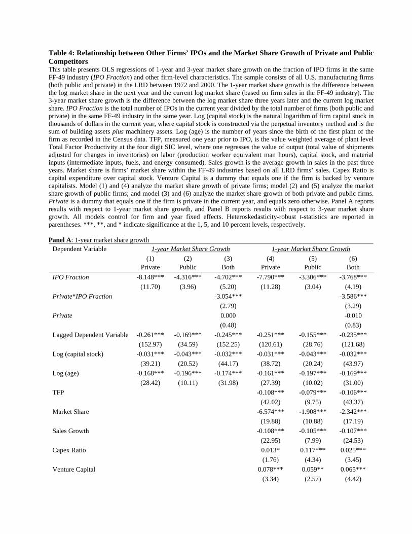
Table 4: Relationship between Other Firms’ IPOs and the Market Share Growth of Private and Public Competitors This table presents OLS regressions of 1-year and 3-year market share growth on the fraction of IPO firms in the same FF-49 industry (IPO Fraction) and other firm-level characteristics. The sample consists of all U.S. manufacturing firms (both public and private) in the LRD between 1972 and 2000. The 1-year market share growth is the difference between the log market share in the next year and the current log market share (based on firm sales in the FF-49 industry). The 3-year market share growth is the difference between the log market share three years later and the current log market share. IPO Fraction is the total number of IPOs in the current year divided by the total number of firms (both public and private) in the same FF-49 industry in the same year. Log (capital stock) is the natural logarithm of firm capital stock in thousands of dollars in the current year, where capital stock is constructed via the perpetual inventory method and is the sum of building assets plus machinery assets. Log (age) is the number of years since the birth of the first plant of the firm as recorded in the Census data. TFP, measured one year prior to IPO, is the value weighted average of plant level Total Factor Productivity at the four digit SIC level, where one regresses the value of output (total value of shipments adjusted for changes in inventories) on labor (production worker equivalent man hours), capital stock, and material inputs (intermediate inputs, fuels, and energy consumed). Sales growth is the average growth in sales in the past three years. Market share is firms’ market share within the FF-49 industries based on all LRD firms’ sales. Capex Ratio is capital expenditure over capital stock. Venture Capital is a dummy that equals one if the firm is backed by venture capitalists. Model (1) and (4) analyze the market share growth of private firms; model (2) and (5) analyze the market share growth of public firms; and model (3) and (6) analyze the market share growth of both private and public firms. Private is a dummy that equals one if the firm is private in the current year, and equals zero otherwise. Panel A reports results with respect to 1-year market share growth, and Panel B reports results with respect to 3-year market share growth. All models control for firm and year fixed effects. Heteroskedasticity-robust t-statistics are reported in parentheses. ***, **, and * indicate significance at the 1, 5, and 10 percent levels, respectively. Panel A: 1-year market share growth

Dependent Variable 1-year Market Share Growth 1-year Market Share Growth (1) (2) (3) (4) (5) (6) Private Public Both Private Public Both

IPO Fraction -8.148*** -4.316*** -4.702*** -7.790*** -3.306*** -3.768***

(11.70) (3.96) (5.20) (11.28) (3.04) (4.19)

Private*IPO Fraction -3.054*** -3.586***

(2.79) (3.29)

Private 0.000 -0.010

(0.48) (0.83)

Lagged Dependent Variable -0.261*** -0.169*** -0.245*** -0.251*** -0.155*** -0.235***

(152.97) (34.59) (152.25) (120.61) (28.76) (121.68)

Log (capital stock) -0.031*** -0.043*** -0.032*** -0.031*** -0.043*** -0.032***

(39.21) (20.52) (44.17) (38.72) (20.24) (43.97)

Log (age) -0.168*** -0.196*** -0.174*** -0.161*** -0.197*** -0.169***

(28.42) (10.11) (31.98) (27.39) (10.02) (31.00)

TFP -0.108*** -0.079*** -0.106***

(42.02) (9.75) (43.37)

Market Share -6.574*** -1.908*** -2.342***

(19.88) (10.88) (17.19)

Sales Growth -0.108*** -0.105*** -0.107***

(22.95) (7.99) (24.53)

Capex Ratio 0.013* 0.117*** 0.025***

(1.76) (4.34) (3.45)

Venture Capital 0.078*** 0.059** 0.065***

(3.34) (2.57) (4.42)

Constant 0.501*** 0.640*** 0.338*** 0.332*** 0.657*** 0.357***

(26.30) (20.92) (31.86) (38.28) (21.33) (33.67)

Observations 439224 48463 487687 437140 48297 485437

R-squared 0.08 0.05 0.07 0.09 0.05 0.08

Panel B: 3-year market share growth Dependent Variable 3-year Market Share Growth 3-year Market Share Growth (1) (2) (3) (4) (5) (6) Private Public Both Private Public Both

IPO Fraction -10.789*** -5.091*** -5.060*** -10.115*** -4.349*** -4.659***

(7.08) (3.08) (3.39) (6.77) (2.71) (3.18)

Private*IPO Fraction -5.561*** -5.243***

(2.76) (2.66)

Private 0.000 -0.010

(0.11) (1.04)

Lagged Dependent Variable -0.331*** -0.301*** -0.317*** -0.283*** -0.236*** -0.273***

(104.91) (50.42) (113.95) (70.98) (31.93) (77.92)

Log (capital stock) -0.110*** -0.123*** -0.113*** -0.096*** -0.096*** -0.096***

(55.57) (31.50) (64.43) (47.44) (24.41) (54.09)

Log (age) -0.388*** -0.447*** -0.402*** -0.332*** -0.258*** -0.321***

(15.91) (8.39) (18.56) (13.83) (4.96) (15.07)

TFP -0.114*** -0.092*** -0.115***

(19.26) (7.50) (21.45)

Market Share -107.161*** -69.420*** -77.339***

(50.95) (38.50) (59.95)

Sales Growth 0.035** 0.136*** 0.069***

(2.41) (5.27) (5.45)

Capex Ratio 0.096*** 0.050 0.088***

(4.74) (1.21) (4.76)

Venture Capital 0.226*** 0.060* 0.126***

(5.50) (1.81) (5.16)

Constant 1.899*** 2.057*** 2.042*** 1.778*** 1.898*** 1.851***

(24.39) (23.84) (29.05) (23.24) (22.50) (26.78)

Observations 120990 32790 153780 120512 32717 153229

R-squared 0.14 0.13 0.14 0.16 0.17 0.16

Table 5: Total Factor Productivity (TFP), Industry IPO Clusteredness, and the Order of Going Public in a Wave This table presents OLS regressions of total factor productivity (TFP) on the three measures of industry IPO clusteredness and the three measures of the order of going public within an IPO wave. The sample consists of U.S. manufacturing firms in the LRD that went public between 1972 and 2000. TFP is the value weighted average of plant level Total Factor Productivity at the four digit SIC level, where one regresses the value of output (total value of shipments adjusted for changes in inventories) on labor (production worker equivalent man hours), capital stock, and material inputs (intermediate inputs, fuels, and energy consumed). The three industry IPO clusteredness measures and the three measures for the order of going public within an IPO wave are defined as in Table 1. Log (capital stock) is the natural logarithm of firm capital stock in thousands of dollars, where capital stock is constructed via the perpetual inventory method and is the sum of building assets plus machinery assets. Log (age) is the number of years since the birth of the first plant of the firm as recorded in the Census data. Years from IPO year are a series of dummies to indicate the gap between the current year and the IPO year of the firm. Model (1) to (3) studies the TFP of IPO firms only in the years before going public, while the rest of the models study the TFP of IPO firms in all years before and after going public. Panel A presents the results for the three measures of industry IPO clusteredness and Panel B presents the results for the three measures of the order of going public within an IPO wave. Panel A analyzes all firms that went public during the sample period, while Panel B analyzes only firms that went public within IPO waves that include at least 5 same-industry IPOs. All models control for industry (FF-49 level) and IPO-year fixed effect. White standard errors, clustered at the firm level, adjusted for possible correlation within the cluster (Rogers standard errors) are reported. Heteroskedasticity-robust t-statistics are reported in parentheses. ***, **, and * indicate significance at the 1, 5, and 10 percent levels, respectively.

Panel A: TFP and IPO clusteredness

Dependent Variable: Total Factor Productivity (TFP)

Years Before Going Public

Years Before and After Going Public

(1) (2) (3) (4) (5) (6) (7) (8) (9) (10) (11) (12) IPONUM -0.010 -0.008*** -0.004** -0.004** (1.60) (2.78) (2.22) (2.55) IPONUM/Same Industry Vol. -3.498** -3.544** -1.602** -1.883** (2.02) (2.45) (2.15) (2.49) IPONUM/Same Window Vol. -2.520** -2.367** -1.019** -0.855* (2.01) (2.44) (2.13) (1.71) Lagged Dependent Variable 0.563*** 0.562*** 0.563*** 0.561*** 0.563*** 0.562*** (31.42) (31.35) (31.30) (31.21) (31.48) (31.37)Log (capital stock) 0.011** 0.011** 0.011** 0.007*** 0.003** 0.003** 0.007*** 0.003** 0.004** 0.007*** 0.003** 0.004** (2.29) (2.39) (2.30) (2.78) (2.32) (2.37) (2.90) (2.38) (2.42) (2.87) (2.38) (2.50) Log (age) 0.020 0.020 0.020 0.010 0.000 0.010 0.010 0.000 0.010 0.010 0.010 0.010 (0.90) (0.85) (0.81) (0.64) (0.38) (1.32) (0.61) (0.34) (1.33) (0.92) (0.59) (1.35) Constant -0.020 0.020 0.030 0.050 0.000 0.209*** 0.086* 0.020 0.188*** 0.088* 0.020 0.149*** (0.34) (0.30) (0.51) (1.31) (0.09) (3.91) (1.78) (0.52) (3.85) (1.89) (0.46) (3.39) Years from IPO Year No No No No No Yes No No Yes No No Yes Observations 3274 3274 3274 7017 6324 6324 7017 6324 6324 7017 6324 6324 R-squared 0.06 0.07 0.06 0.05 0.35 0.36 0.05 0.35 0.36 0.05 0.35 0.36

Panel B: TFP and the order of going public in an IPO wave Dependent Variable: Total Factor Productivity (TFP)

Years Before Going Public

Years Before and After Going Public

(1) (2) (3) (4) (5) (6) (7) (8) (9) (10) (11) (12) EARLINESS -0.063*** -0.049*** -0.027** -0.027** (2.81) (2.67) (2.44) (2.34) ORDER / Median ORDER -0.120** -0.093** -0.052** -0.051** (2.58) (2.51) (2.23) (2.12) Log (ORDER) -0.088** -0.072*** -0.038** -0.038** (2.52) (2.72) (2.31) (2.23) Lagged Dependent Variable 0.500*** 0.500*** 0.500*** 0.500*** 0.500*** 0.500*** (17.45) (17.20) (17.39) (17.14) (17.43) (17.15)Log (capital stock) 0.000 0.000 0.000 0.010 0.000 0.000 0.010 0.000 0.000 0.010 0.000 0.000 (0.30) (0.27) (0.11) (1.23) (1.15) (1.15) (1.19) (1.12) (1.11) (1.06) (1.02) (1.00) Log (age) 0.059** 0.058** 0.058** 0.041* 0.010 0.020 0.041* 0.010 0.020 0.039* 0.010 0.020 (2.26) (2.23) (2.20) (1.89) (0.74) (1.09) (1.88) (0.73) (1.09) (1.78) (0.67) (1.03) Constant 0.220 0.260 0.330 0.349*** 0.090 -0.030 0.380*** 0.103* 0.211** 0.488*** 0.161** 0.090 (1.12) (1.30) (1.62) (3.72) (1.51) (0.08) (4.05) (1.78) (2.43) (4.57) (2.33) (0.30) Years from IPO Year No No No No No Yes No No Yes No No Yes Observations 1607 1607 1607 3274 2920 2920 3274 2920 2920 3274 2920 2920 R-squared 0.22 0.22 0.22 0.16 0.38 0.39 0.16 0.38 0.39 0.16 0.38 0.39

Table 6: Post-IPO Operating Performance, Industry Clusteredness of IPOs, and the Order of Going Public in an IPO Wave This table presents OLS regressions of post-IPO operating performance on three measures of industry IPO clusteredness (“hotness” of the IPO market) and the three measures for the order of going public within an IPO wave. The post-IPO operating performance measure is defined as the return on assets (ROA) for the first fiscal year after the IPO date (COMPUSTAT DATA13/DATA6). The three industry IPO clusteredness measures and the three measures for the order of going public within an IPO wave are defined as in Table 1. The other independent variables include: logarithm of firm’s market capital (DATA199*DATA25) at the first fiscal year end after the IPO; IPO’s offer price; a dummy variable showing whether the issuer is backed by venture capitalists (equals 1 if yes); the initial return of the IPO firm’s stock (difference between the first closing price and the offer price, divided by the offer price); logarithm of total IPO proceeds; percentage of secondary shares sold in the IPO; firms’ market share within the FF-49 industries based on all Compustat firms’ net sales (DATA12); percentage of shares owned by institutional investors right after the IPO; logarithm of firm’s age at IPO date (number of years between the firm’s founding year and the IPO year); capital expenditure scaled by firm’s net property, plant, and equipment (DATA128/DATA8); research & development expenses scaled by total net assets (DATA46/DATA6); and the reputation for underwriters. IPO Month Market Return is the total monthly return on the value-weighted portfolio of all NYSE, AMEX, and NASDAQ stocks for the month during which the firm went public. IPO Month Market Volatility is computed as the standard deviation of daily value weighted market returns for the month during which the firm went public. IPO Month MB Ratio is the sum of market values of equity across all ordinary common shares divided by the sum of the most recent book values of equity for the month during which the firm went public. The first four columns in each panel analyze all firms that went public during the sample period, while the latter four columns analyze only firms that went public within IPO waves that include at least 5 same-industry IPOs. All models control for industry (FF-49 level) and IPO-year fixed effect. White standard errors, clustered at the industry level, adjusted for possible correlation within the cluster (Rogers standard errors) are reported. Heteroskedasticity-robust t-statistics are reported in parentheses. ***, **, and * indicate significance at the 1, 5, and 10 percent levels, respectively.

Dependent Variable: ROA (1) (2) (3) (4) (5) (6) IPONUM -0.0016*** (-4.16) IPONUM/Same Industry Vol. -0.6741*** (-3.09) IPONUM/Same Window Vol. -0.2340*** (-4.72) EARLINESS -0.0076** (-2.40) ORDER / Median ORDER -0.0160** (-2.71) Log (ORDER) -0.0086*** (-3.00) Log (market cap) 0.0579*** 0.0573*** 0.0579*** 0.0543*** 0.0544*** 0.0542*** (8.61) (8.58) (8.64) (8.20) (8.21) (8.07) Offer Price 0.0033** 0.0033** 0.0034** 0.0035** 0.0035** 0.0036** (2.59) (2.56) (2.56) (2.13) (2.12) (2.25) Dummy for VC backing -0.0254** -0.0270** -0.0256** -0.0373*** -0.0374*** -0.0370*** (-2.41) (-2.56) (-2.48) (-3.51) (-3.52) (-3.46) Initial Return (percent) -0.0004*** -0.0004*** -0.0004*** -0.0003*** -0.0003*** -0.0003*** (-4.89) (-5.05) (-4.80) (-3.42) (-3.45) (-3.32) Log (IPO proceeds) -0.0747*** -0.0732*** -0.0749*** -0.0815*** -0.0817*** -0.0818***

(-7.72) (-7.68) (-7.71) (-6.90) (-6.93) (-6.90) Percent of Secondary Shares 0.2032*** 0.2031*** 0.2025*** 0.2367*** 0.2365*** 0.2382*** (7.14) (7.00) (7.04) (7.19) (7.22) (7.32) Market Share -0.2182 -0.2513 -0.2185 0.2956 0.2926 0.2398 (-1.00) (-1.08) (-1.00) (0.51) (0.50) (0.41) Percent of Institutional Holding 0.1165*** 0.1196*** 0.1176*** 0.1392*** 0.1391*** 0.1396*** (5.83) (5.91) (6.00) (4.37) (4.36) (4.42) Log (firm age at IPO date) 0.0317*** 0.0312*** 0.0315*** 0.0316*** 0.0315*** 0.0318*** (5.58) (5.64) (5.62) (5.33) (5.30) (5.34) CapEx/PPE -0.0618*** -0.0638*** -0.0614*** -0.0827*** -0.0829*** -0.0812*** (-4.76) (-4.96) (-4.71) (-5.76) (-5.78) (-5.52) R&D/Assets -1.0463*** -1.0528*** -1.0394*** -1.0647*** -1.0644*** -1.0539*** (-8.84) (-8.98) (-8.88) (-8.82) (-8.76) (-8.71) Underwriter Reputation 0.0095*** 0.0092*** 0.0094*** 0.0111*** 0.0111*** 0.0111*** (4.93) (4.81) (5.01) (4.85) (4.84) (4.90) IPO Month Market Return IPO Month Market Volatility IPO Month MB Ratio Constant -0.0795** -0.0595* -0.0768** -0.1616** -0.1550** -0.1592** (-2.15) (-1.72) (-2.11) (-2.69) (-2.61) (-2.61) Observations 3259 3259 3259 2321 2321 2321 R-squared 0.556 0.555 0.557 0.581 0.581 0.581

Table 7: Post-IPO Cash Balance, Industry Clusteredness of IPOs, and the Order of Going Public in an IPO Wave This table presents OLS regressions of post-IPO cash balance on the three measures of industry IPO clusteredness and the three measures of the order of going public within an IPO wave. The post-IPO cash balance is measured in two ways: Panel A uses the increase in cash and cash equivalents scaled by total net assets (DATA274/DATA6) as the dependent variable; and Panel B uses cash and short-term investments scaled by total net assets (DATA1/DATA6). The three industry IPO clusteredness measures and the three measures for the order of going public within an IPO wave are defined as in Table 1. The other independent variables include: logarithm of firm’s market capital (DATA199*DATA25) at the first fiscal year end after the IPO; IPO’s offer price; a dummy variable showing whether the issuer is backed by venture capitalists (equals 1 if yes); the initial return of the IPO firm’s stock (difference between the first closing price and the offer price, divided by the offer price); logarithm of total IPO proceeds; percentage of secondary shares sold in the IPO; firms’ market share within the FF-49 industries based on all Compustat firms’ net sales (DATA12); percentage of shares owned by institutional investors right after the IPO; logarithm of firm’s age at IPO date (number of years between the firm’s founding year and the IPO year); and the reputation for underwriters. The first three columns in each panel analyze all firms that went public during the sample period, while the latter three columns analyze only firms that went public within IPO waves that include at least 5 same-industry IPOs. All models control for industry (FF-49 level) and IPO-year fixed effect. White standard errors, clustered at the industry level, adjusted for possible correlation within the cluster (Rogers standard errors) are reported. Heteroskedasticity-robust t-statistics are reported in parentheses. ***, **, and * indicate significance at the 1, 5, and 10 percent levels, respectively.

Panel A: The increase in cash and cash equivalents after the IPO scaled by total net assets

Dependent Variable: Increase in cash and cash equivalents after the IPO scaled by assets (1) (2) (3) (4) (5) (6) IPONUM 0.0013* (1.83) IPONUM/Same Industry Vol. 0.4190** (2.12) IPONUM/Same Window Vol. 0.0319 (0.40) EARLINESS 0.0201*** (3.42) ORDER / Median ORDER 0.0387*** (3.53) Log (ORDER) 0.0182*** (4.09) Log (market cap) 0.0212*** 0.0216*** 0.0214*** 0.0214*** 0.0211*** 0.0214*** (5.56) (5.52) (5.41) (4.88) (4.82) (5.02) Offer Price 0.0020** 0.0020** 0.0021** 0.0022 0.0021 0.0018 (2.15) (2.17) (2.20) (1.52) (1.52) (1.31) Dummy for VC backing 0.0323*** 0.0339*** 0.0335*** 0.0339*** 0.0341*** 0.0322*** (3.65) (3.94) (3.81) (3.21) (3.23) (3.10) Initial Return (percent) 0.0003* 0.0003* 0.0003* 0.0002 0.0002 0.0002 (1.73) (1.71) (1.75) (1.19) (1.21) (1.15) Log (IPO proceeds) -0.0426*** -0.0436*** -0.0429*** -0.0423*** -0.0420*** -0.0412***

(-6.09) (-6.39) (-6.15) (-4.38) (-4.36) (-4.40) Percent of Secondary Shares 0.0054 0.0060 0.0054 -0.0085 -0.0082 -0.0133 (0.32) (0.36) (0.33) (-0.37) (-0.35) (-0.60) Market Share -0.5441 -0.5264 -0.5640 -1.7897*** -1.7628*** -1.6637*** (-1.09) (-1.05) (-1.11) (-3.91) (-3.92) (-3.77) Percent of Institutional Holding 0.0083 0.0055 0.0058 0.0116 0.0116 0.0110 (0.45) (0.29) (0.32) (0.54) (0.54) (0.53) Log (firm age at IPO date) -0.0273*** -0.0271*** -0.0272*** -0.0173*** -0.0173*** -0.0178*** (-6.54) (-6.49) (-6.48) (-3.88) (-3.86) (-3.94) Underwriter Reputation -0.0134*** -0.0132*** -0.0132*** -0.0104*** -0.0104*** -0.0105*** (-5.30) (-5.26) (-5.29) (-3.58) (-3.61) (-3.52) Constant 0.3419*** 0.3316*** 0.3464*** 0.1936*** 0.1832*** 0.1970*** (8.83) (8.50) (8.79) (5.34) (5.01) (5.05) Observations 3315 3315 3315 2362 2362 2362 R-squared 0.208 0.207 0.206 0.194 0.194 0.194

Panel B: The cash and short-term investments after the IPO scaled by total net assets Dependent Variable: Cash and short-term investments after the IPO scaled by assets (1) (2) (3) (4) (5) (6) IPONUM 0.0021*** (2.93) IPONUM/Same Industry Vol. 0.8378*** (2.74) IPONUM/Same Window Vol. 0.1948** (2.07) EARLINESS 0.0104 (1.37) ORDER / Median ORDER 0.0218 (1.60) Log (ORDER) 0.0220*** (3.38) Log (market cap) 0.0168*** 0.0175*** 0.0170*** 0.0114* 0.0113* 0.0121* (2.82) (2.92) (2.84) (1.75) (1.74) (1.83) Offer Price 0.0043** 0.0043** 0.0043** 0.0044** 0.0044** 0.0042** (2.44) (2.42) (2.47) (2.03) (2.04) (2.04) Dummy for VC backing 0.0998*** 0.1024*** 0.1007*** 0.1000*** 0.1001*** 0.0982*** (8.27) (8.65) (8.29) (8.19) (8.20) (7.96) Initial Return (percent) 0.0004*** 0.0004*** 0.0004*** 0.0003** 0.0003** 0.0003** (3.20) (3.09) (3.11) (2.29) (2.32) (2.22)

Log (IPO proceeds) -0.0637*** -0.0656*** -0.0636*** -0.0604*** -0.0603*** -0.0594*** (-6.08) (-6.67) (-6.11) (-3.96) (-3.97) (-3.91) Percent of Secondary Shares 0.0005 0.0017 0.0010 -0.0084 -0.0081 -0.0125 (0.019) (0.063) (0.037) (-0.23) (-0.23) (-0.36) Market Share -0.6013 -0.5579 -0.6163 -2.1010*** -2.0927*** -2.0575*** (-0.95) (-0.88) (-0.97) (-3.04) (-3.03) (-3.00) Percent of Institutional Holding -0.0734*** -0.0780*** -0.0758*** -0.0726** -0.0724** -0.0718** (-2.90) (-3.08) (-3.00) (-2.19) (-2.19) (-2.16) Log (firm age at IPO date) -0.0453*** -0.0450*** -0.0451*** -0.0407*** -0.0406*** -0.0407*** (-6.64) (-6.65) (-6.61) (-5.91) (-5.87) (-5.86) Underwriter Reputation -0.0021 -0.0018 -0.0020 0.0030 0.0030 0.0025 (-0.56) (-0.49) (-0.52) (0.78) (0.78) (0.64) Constant 0.4603*** 0.4377*** 0.4613*** 0.4564*** 0.4478*** 0.4173*** (8.72) (8.26) (8.68) (8.23) (7.94) (7.73) Observations 3315 3315 3315 2362 2362 2362 R-squared 0.481 0.479 0.479 0.475 0.475 0.479

Table 8: Industry Concentration, Post-IPO Operating Performance, Industry Clusteredness of IPOs, and the Order of Going Public in an IPO Wave This table presents OLS regressions of post-IPO operating performance on industry concentration, the three measures of industry IPO clusteredness, the three measures of the order of going public within an IPO wave, and the interaction between concentration and IPO clusteredness and order measures. The post-IPO operating performance measure is defined as the return on assets (ROA) for the first fiscal year after the IPO date (COMPUSTAT DATA13/DATA6). Industry concentration is the Herfindahl-Hirschman Index (HHI) calculated based on all Compustat firms’ post-IPO total net assets within a certain FF-49 industry. The three industry IPO clusteredness measures and the three measures for the order of going public within an IPO wave are defined as in Table 1. The other independent variables include: logarithm of firm’s market capital (DATA199*DATA25) at the first fiscal year end after the IPO; IPO’s offer price; a dummy variable showing whether the issuer is backed by venture capitalists (equals 1 if yes); the initial return of the IPO firm’s stock (difference between the first closing price and the offer price, divided by the offer price); logarithm of total IPO proceeds; percentage of secondary shares sold in the IPO; firms’ market share within the FF-49 industries based on all Compustat firms’ net sales (DATA12); percentage of shares owned by institutional investors right after the IPO; logarithm of firm’s age at IPO date (number of years between the firm’s founding year and the IPO year); capital expenditure scaled by firm’s net property, plant, and equipment (DATA128/DATA8); research & development expenses scaled by total net assets (DATA46/DATA6); and the reputation for underwriters. Panel A analyzes all firms that went public during the sample period, while Panel B analyzes only firms that went public within IPO waves that include at least 5 same-industry IPOs. All models control for industry (FF-49 level) and IPO-year fixed effect. White standard errors, clustered at the industry level, adjusted for possible correlation within the cluster (Rogers standard errors) are reported. Heteroskedasticity-robust t-statistics are reported in parentheses. ***, **, and * indicate significance at the 1, 5, and 10 percent levels, respectively. Panel A: Industry concentration and IPO clusteredness

Dependent Variable: ROA (1) (2) (3) IPONUM -0.0020*** (-3.33) Herfindahl Index * IPONUM 0.0064 (1.37) IPONUM/Same Industry Vol. (IPONUM_1) -0.8502** (-2.58) Herfindahl Index * IPONUM_1 1.5138 (1.07) IPONUM/Same Window Vol. (IPONUM_2) -0.3086*** (-4.49) Herfindahl Index * IPONUM_2 1.1343*** (3.02) Herfindahl Index -0.0730* -0.0657 -0.0966** (-1.84) (-0.92) (-2.34) Log (market cap) 0.0580*** 0.0572*** 0.0581*** (8.60) (8.56) (8.61) Offer Price 0.0033** 0.0033** 0.0034** (2.60) (2.57) (2.58) Dummy for VC backing -0.0253** -0.0270** -0.0258** (-2.44) (-2.56) (-2.50) Initial Return (percent) -0.0004*** -0.0004*** -0.0004*** (-5.21) (-5.01) (-5.12) Log (IPO proceeds) -0.0748*** -0.0733*** -0.0752*** (-7.76) (-7.64) (-7.73) Percent of Secondary Shares 0.2019*** 0.2028*** 0.2012*** (7.13) (7.10) (7.04) Market Share -0.2280 -0.2478 -0.2374 (-1.06) (-1.09) (-1.10) Percent of Institutional Holding 0.1162*** 0.1194*** 0.1171*** (5.95) (6.02) (6.13) Log (firm age at IPO date) 0.0317*** 0.0312*** 0.0315***

(5.56) (5.63) (5.61) CapEx/PPE -0.0623*** -0.0639*** -0.0618*** (-4.81) (-4.94) (-4.75) R&D/Assets -1.0484*** -1.0527*** -1.0413*** (-8.94) (-9.03) (-9.01) Underwriter Reputation 0.0095*** 0.0092*** 0.0095*** (4.96) (4.82) (5.11) Constant -0.0627* -0.0476 -0.0557 (-1.78) (-1.59) (-1.64) Observations 3259 3259 3259 R-squared 0.556 0.555 0.557

Panel B: Industry concentration and the order of going public in an IPO wave Dependent Variable: ROA (1) (2) (3) EARLINESS -0.0152*** (-3.62) Herfindahl Index * EARLINESS 0.0750*** (3.40) ORDER / Median ORDER (ORDER_N) -0.0271*** (-3.46) Herfindahl Index * ORDER_N 0.1092** (2.57) Log (ORDER) -0.0143*** (-2.91) Herfindahl Index * Log (ORDER) 0.0633** (2.29) Herfindahl Index -0.1827*** -0.1809** -0.2266*** (-2.96) (-2.50) (-4.05) Log (market cap) 0.0541*** 0.0543*** 0.0542*** (8.13) (8.17) (7.96) Offer Price 0.0034** 0.0034** 0.0037** (2.08) (2.07) (2.32) Dummy for VC backing -0.0373*** -0.0374*** -0.0370*** (-3.54) (-3.54) (-3.48) Initial Return (percent) -0.0003*** -0.0003*** -0.0003*** (-3.39) (-3.40) (-3.50) Log (IPO proceeds) -0.0808*** -0.0810*** -0.0818*** (-6.90) (-6.94) (-6.96) Percent of Secondary Shares 0.2380*** 0.2376*** 0.2384*** (7.21) (7.24) (7.34) Market Share 0.2341 0.2381 0.1824 (0.41) (0.42) (0.32) Percent of Institutional Holding 0.1370*** 0.1371*** 0.1383*** (4.26) (4.26) (4.38) Log (firm age at IPO date) 0.0317*** 0.0316*** 0.0319*** (5.33) (5.28) (5.33) CapEx/PPE -0.0825*** -0.0830*** -0.0818*** (-5.78) (-5.81) (-5.60) R&D/Assets -1.0615*** -1.0619*** -1.0519*** (-8.96) (-8.85) (-8.79) Underwriter Reputation 0.0110*** 0.0110*** 0.0112*** (4.90) (4.85) (4.97) Constant -0.1461** -0.1400** -0.1438** (-2.46) (-2.40) (-2.31) Observations 2321 2321 2321 R-squared 0.582 0.582 0.582