iowa state university - core.ac.uk · according to summary report of iowa lake valuation project...
TRANSCRIPT

IOWA STATE UNIVERSITY
Department of Economics Working Papers Series
Ames, Iowa 50011
Iowa State University does not discriminate on the basis of race, color, age, religion, national origin, sexual orientation, gender identity, sex, marital status, disability, or status as a U.S. veteran. Inquiries can be directed to the Director of Equal Opportunity and Diversity, 3680 Beardshear Hall, (515) 294-7612.
The Role of Water Quality Perceptions in Modeling Lake Recreation Demand
Yongsik Jeon, Joseph A. Herriges, Catherine L. Kling, John Downing
November 2005
Working Paper # 05032
The Role of Water Quality Perceptions in Modeling Lake Recreation Demand
by
Yongsik Jeon SK Research Institute
Joseph A. Herriges and Catherine L. Kling Department of Economics, Iowa State University
John Downing Department of Ecology, Evolution and Organismal Biology, Iowa State University
Preliminary Draft – Please do no quote without permission
November 14, 2005
I. Introduction
According to the U.S. Environmental Protection Agency’s (the U.S. EPA) most
recent national water quality inventory (2000), 45% of the lake acres are impaired. This
assessment is based on physical water quality measures. In Iowa, the problem is no better.
Indeed, over half of the 132 lakes included in the Iowa Lake Valuation project are on the
U.S. EPA's impaired list (EPA water quality inventory for the state of Iowa, 2003).
Despite the fact that physical measures indicate water quality concerns in the state,
these same lakes are used extensively by Iowans for recreational boating, fishing, swimming,
etc. According to summary report of Iowa Lake Valuation project (Azevedo et al. 2003),
approximately 62% of all Iowa households visited one of the 132 lakes in 2002, with an
average of eight day-trips per year. Yet these same respondents indicated that water quality
was the most important factor they consider when choosing a lake for recreation. Clear Lake
in north-central Iowa is the center of many activities and is especially lively in the summer
months despite being on the lists of impaired lakes. Fishermen, recreational boaters,
swimmers and beach users all frequent the lake. As Ditton and Goodale (1973) suggests,
physical water quality is not necessarily the qualities that attract or deter recreation users.
The question is what form of quality attributes drives individual's site choice
decision: physical measures or quality perceptions? How do these affect trip behavior? This
paper utilizes detailed data on trip behavior and water quality perceptions collected from
Iowa Lake Survey 2003 and physical quality measures collected by the Iowa State University
Limnologist laboratory to investigate which measures have the greatest impact on the site
choice decision.
A related issue of interest is whether individual water quality perceptions are
correlated with the available physical measures, i.e., to what extent do individuals have
1
accurate perceptions of quality? Biases in quality perceptions are of interest to policy makers
from the standpoint of welfare analysis. If perceptions do influence recreation trip behavior,
but these perceptions differ from the corresponding physical measures (or the U.S. EPA's
categorization of them), the changes to the physical water quality of a lake may have
unintended impacts of lake usage and the corresponding welfare calculations will be in error.
The remainder of this paper is divided into five sections. Section II provides a review
of the existing literature on water quality perceptions. Section III describes the trip behavior
and quality assessments data collected in the Iowa Lake Survey 2003 and physical measures
of 131 Iowa lakes collected by the Limnology Lab at Iowa State University. The repeated
mixed logit model (RXL) to be used in the analysis is described in Section IV. Welfare
estimation is discussed in Section V. Section VI provides some preliminary conclusions and
an outline of the remaining research issues.
II. Literature Review
Recent studies of recreation demand show that physical water quality measures
significantly impact the site choice decision. Phaneuf, Herriges, and Kling (2000) estimated a
Kuhn-Tucker model analyzing angler behavior in the Great Lakes. They include catch rates
for particular fish species of interest as well as a toxin measure derived from the average
toxin levels given in a study by De Vault et al. (1989). The authors find that the toxin level, a
measure of the presence of environmental contaminants, significantly influences the
recreation decision.
Egan (2003) estimates the demand for day-trips to 129 Iowa lakes using data from the
first year of the Iowa Lakes valuation project. Included in his analysis are 11 physical quality
measures (secchi depth, chlorophyll, nitrogen, total phosphorus, etc.) and a series of other
2
lake specific characteristics (ramp, wake, facilities, state park designation etc). His results
show that individuals do respond to physical quality characteristics in choosing where to
recreate. Egan (2003) goes onto estimate the willingness of Iowans to pay to improve the
physical water quality levels in the state.
The Egan (2003) analysis, however, does not explore the crucial link between the
physical water quality measures and individual perceptions of them. Researchers often argue
that choices are made on the basis of perceptions. Yet, there has been relatively little use of
perceptions of quality attributes in recreation demand modeling in the past due to the cost of
collecting individual perception information. One of the few exceptions is Adamowicz et al.
(1997), which examines perceptual and objective quality attribute measures in discrete choice
models of moose hunting site choice behavior. They employed data collected from
recreational moose hunters in Alberta, Canada including actual and perceived hunting site
attributes (access, moose population and congestion) of hunters. Their analysis shows that the
model with perceptual attributes of hunting place outperforms that of objective quality
attribute, though only modestly. Two scenarios are considered for welfare estimation: one
involving closure of a site and the other involving a change in perceptions to the agency's
objective measure for those individuals who have perceptions that are lower than the target
level. The authors find that welfare estimates obtained using “perception” model are less than
that from “objective quality” model for both scenarios. This is because individuals are
assumed to experience a welfare gain only when their perception of the site quality is below
the agency target.
3
III. Data and Survey Results
Two sources of data will be used in this paper: results from the 2003 Iowa Lakes
Survey and physical water quality measures collected by the ISU Limnology Lab. These data
sources are described in turn in the following two subsections.
A. The 2003 Iowa Lakes Survey
The 2003 Iowa Lakes Survey is the second year survey in a four year study, jointly
funded by the Iowa Department of Natural Resources and the USEPA, aimed at
understanding recreational lake usage in Iowa and the value placed on water quality in the
state. The survey was sent by direct mail in January of 2004 to a random sample 8,000
Iowans, collecting information on their recreation behavior as well as their assessment of the
Iowan's 131 principal lakes. Standard follow-up procedures were used to encourage a high
response rate to the survey (see, e.g., Dillman, 1978, 2000), including a postcard reminder
mailed two weeks after the initial mailing and a second copy of the survey mailed one month
later. In addition, survey respondents were provided with a $10 incentive for completing the
survey.
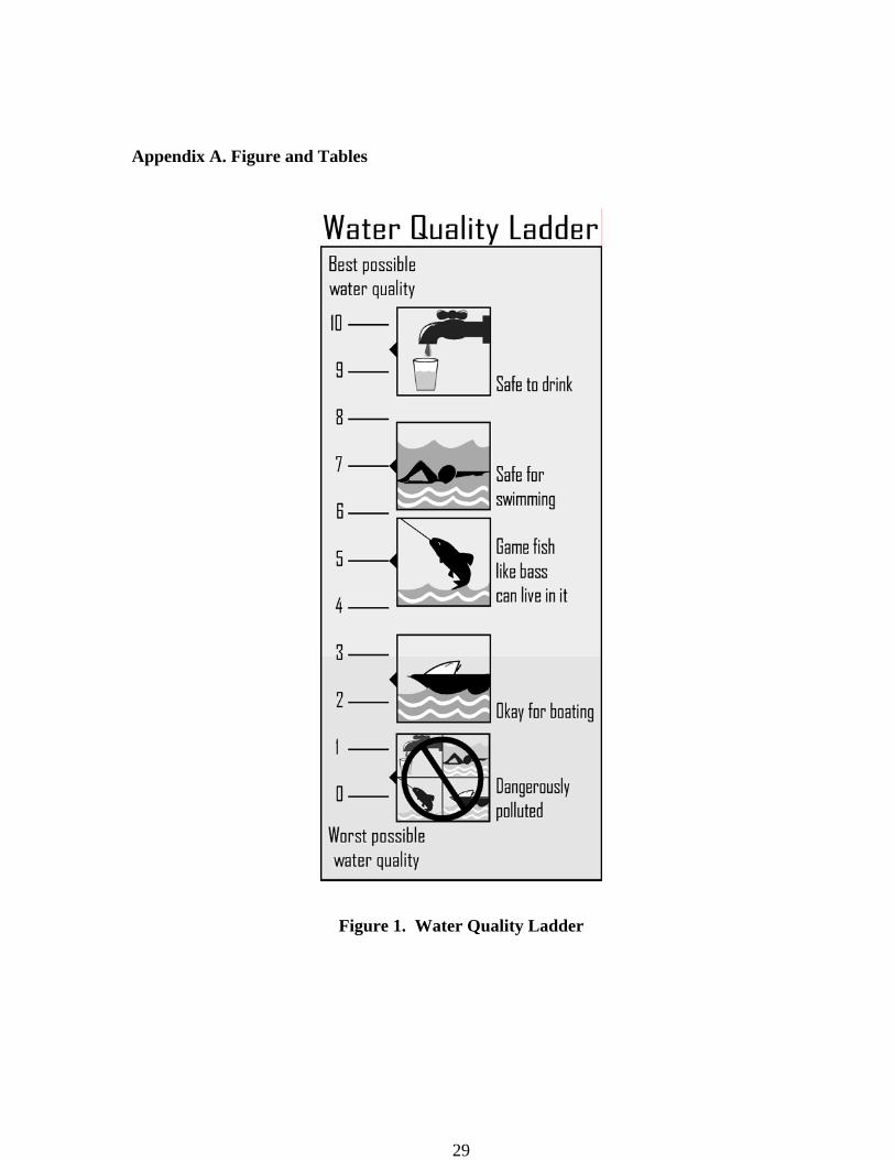
The survey itself has three major sections. The first section (pp. 3-7) asks respondents
to report both how frequently they visited each of 131 lakes in the state during 2003 and to
rate those lakes they are familiar with in terms of water quality. The 10-point water quality
ladder (Figure 1) employed by EPA is used in this water quality assessment. The water
quality ladder has been used in the past both to categorize lakes in terms of quality and in
communicating potential water quality improvements (e.g., from "boatable" to "fishable" or
"drinkable"). The second section of the survey (pp. 8-9) consists of dichotomous choice
referendum questions and is not used in this essay. Section three, (pp. 10-11) collects socio-
demographic information, including age, gender, education, etc.
4
A total of 5,281 surveys have been returned. Allowing for the fact that 219 surveys
that were undeliverable and the 61 deceased individuals in the original sample, this
corresponds to a 68% response rate. From the 5,281 completed surveys, the final sample of
5,052 individuals was obtained as follows. Non-Iowans were excluded (47 observations)
based on zip code. Anyone reporting more than 52 total single day trips to the 131 lakes were
excluded as well (182 observations). The analysis below focuses on single day trips only in
order to avoid the complexity of modeling multiple day visits. Defining the number of choice
occasions as 52 trips per year allows one trip to one of the 131 Iowa lakes per week. While
the choice of 52 is arbitrary, it seems a reasonable cut-off for the total number of allowable
single day trips for the season. Invariably some of the respondents who recorded trips greater
52 did in fact take this number of trips. However, since this survey was randomly sent out to
Iowan, some of the recipients live on a lake and it may be those individuals who record
hundreds of "trips" are simply returning to their sleep of residence.
Table 1 lists the summary statistics for trips and the socio-demographic data. The
average number of total single day trips to all 131 lakes is 6.97, ranging from zero to 52 trips
per year. The survey respondents are more likely to be older, male, have a higher income,
and be more educated than the general Iowa population. Schooling is entered as a dummy
variable equaling one if the individual has attended or completed some level of post high
school education.
As indicated above, water quality assessment data were collected by directly asking
the respondents to assign a number between 0 and 10 based on the water quality ladder
(Figure 1) for the lakes they visited in 2003 or considered visiting recently. Water quality
ladder, proposed by Carson and Mitchell (1983), was pictured page by page on the survey
with verbal descriptions. The top of the water quality ladder stands for the best possible
5
quality of water, while the bottom of the ladder stands for the worst. The lowest level is so
polluted that contact with it is dangerous to human health. Water quality that is "boatable"
would not harm an individual if they happened to fall into it for a short time while boating or
sailing. Water quality that is "fishable" is a higher level of quality than "boatable". Although
some kinds of fish can live in boatable water, it is only when water is "fishable" that game
fish like bass can live in it. Finally, "swimmable" water is of a high enough quality that it is
safe to swim in and ingest in small amounts.
The summary statistics for day trips (per capita) and median, mean, and standard
deviation of the water quality perception for each lake are listed in Table 2. The sample size
is 131 lakes. Total day trips per lake is divided by the total number of surveys sent out to the
local zone where a lake is located in order to standardize population size effect on trips. On
average, Iowans took 0.36 trips per capita to each lake last year.
Although some individuals perceived some of lakes were polluted dangerously, most
respondents perceived the 131 lakes to be safe for swimming and boating on average. The
mean water quality assessment ranges across lakes from 4.11 to 6.81. Standard deviation of
the water quality assessment of a lake measured across individuals who rated the lake in
question ranges from 1.06 to 2.42. This suggests that for some lakes, individuals share very
similar perceptions regarding the lake’s quality. For example, for Green Castle Lake
(Marshall County), the standard deviation of water quality perceptions is 1.07 across 35
respondents. For other lakes, such West Lake (Osceola) with a standard deviation of 2.63
across 62 respondents, the water quality perceptions are wide ranging.
An initial question regarding the lake perceptions data is whether or not it influenced
which lakes Iowan visited in 2003. To investigate this, Table 3 lists number of day trips per
capita to the 20 best and 20 worst lakes sorted by their mean water quality assessments.
6
Although some lakes had few respondents assessing their water quality, the mean number of
day trips to the “best” lakes (with a mean assessment of 6.46) is roughly two and a half times
the mean number of trips to the “worst” lakes (which had a mean assessment of 4.89). The
best lakes, of course, do not have uniformly higher visitation rates. Ottumwa Lagoon
(Wapello), Lake Macbride (Johnson), Swan Lake (Carroll) and George Wyth Lake (Black
Hawk) in the “worst” lakes category all have higher visitation rates than Lake Wapello and
Little River Watershed Lake included in the “best” lakes category. More detailed analysis
will be required to tease out other factors influencing recreational site choices, such as
proximity to population centers. However, these aggregate data do suggest that water quality
perception influence the site choice decision.
It should also be noted that high quality assessments do not necessarily imply that the
lake is less contaminated (based on actual physical water quality measures). According to the
list of impaired lakes of Iowa, Lake Meyer, Lake Keomah, Lake Smith, and Lake Icaria are
impaired, even though they have high mean quality assessments. Moreover, four lakes
among worst assessment lakes, including Mitchell Lake, Meyers Lake, Briggs Woods Lake
and George Wyth Lake are not on the list. This implies that individual's perceptions may not
agree with either EPA or physical water quality assessments.1 Correlation coefficients of
mean water quality assessment with the number of day trip and physical water quality
measures are calculated in the following subsection.
C. Physical Quality Measures
Table 4 lists the summary statistics of physical water quality measures. Secchi depth
is a measure for clarity of water surface indicating how far down into the water an object
1 Of course, factors other than physical water quality conditions may play a role in listing a lake on the impaired water quality list.
7
remains visible. Chlorophyll is an indicator of plant biomass or algae and leads to greenness
in the water. Total phosphorus is usually the principal limiting nutrient in Iowa lakes,
meaning it most likely determines algae growth. Three nitrogen levels are provided,
including NH3+NH4 (measuring particular types of nitrogen such as ammonia which can be
toxic), NO3+NO2 (measuring the nitrates in the water), and total nitrogen. Silicon is
important to diatoms which extract it from the water to use as a component of their cell walls.
Diatoms, in turn, are a key food source for marine organisms. The acidity of the water is
measured by "pH" with levels below 6 or above 8 indicating unhealthy lakes. Alkalinity is
the concentration of calcium or calcium carbonate in the water. Plants need carbon to grow
and all carbon comes from alkalinity, therefore alkalinity is an indication of the abundance of
plant life. ISS is the inorganic suspended solids, basically soil and silt in the water due to
erosion. VSS is volatile or organic suspended solids, both measures that will decrease clarity
in the water.
It is evident that considerable variation in physical water quality characteristics is
present across the lakes in Iowa. For example, Secchi depth varies from a low of 0.17 meters
to a high of 8.10 meters and total phosphorus varies from 17 to 384 µg/L, some of the highest
concentrations in the world. All of the physical measures are the average values for the 2003
season. Samples were taken from each lake three times throughout the year, in spring/early
summer, mid-summer, and late summer/fall, to include seasonal variation.
According to EPA's "Nutrient Criteria Technical Guidance Manual (2000)", the four
paramount variables for nutrient criteria are total phosphorus, total nitrogen, chlorophyll, and
secchi depth. Scientists consider inorganic suspended solids and organic suspended solids to
be crucial indicators as well. The question is how close are the perceptions of individuals and
physical measures of EPA's and/or scientists? Further, do EPA’s water quality index and/or
8
scientist’s water quality index explain water quality perception?
EPA’s water quality index used in the water quality ladder is a weighted average of
up to nine quality indices based on physical quality measures including total phosphates
(PO4), total nitrates (NO3), total suspended solids, dissolved oxygen and pH. A water quality
index using the latter five variables are constructed using data from the ISU limnology lab.2
In addition, Carson’s Trophic State Indices (CSTI) for lakes based on secchi depth
(CTSI_SEC), chlorophyll (CTSI_Chla), total phosphorus (CTSI_TP) are provided from the
ISU Limnology Lab.3 As described in Appendix B, a trophic state index is an objective
standard of the trophic state of any body of water whereas the water quality ladder index
represents a subjective judgment by a group of scientist.
Table 5 lists correlation coefficient of quality assessment with several physical
measures, EPA’s water quality index and Trophic State Indices. The correlations are
provided for the sample as a whole and for two subsamples: those reporting that they
engaged in water contact activities (e.g., swimming and jet skiing) and those who did not
(e.g., nature appreciation and picnicking). One might expect those engaged in water contact
activities might be more aware of and/or affected by the physical water quality conditions.
For the sample as a whole, day trips were found to be positively correlated with the
corresponding water quality perception measure. This suggests, as indicated by Table 3, that
overall quality perceptions do influence trip behavior. The overall water quality assessments
also are generally consistent with the actually physical water quality measures. Specifically,
all of the physical measures are negatively correlated with mean water quality assessment
except for secchi depth; clarity of the water has positive relationship with the water quality
2 Appendix A provides details regarding the construction of these water quality indices. 3 For details about Carson’s Trophic State Index, see Appendix B.
9
ladder assessment (0.351). However, the degree of correlation varies by the physical water
quality measure. For example, there is relatively little correlation between the water quality
assessment and the nitrates, chlorophyll and pH. Water quality perceptions also appear to be
correlated with a number of existing water quality indices, based on physical water quality
measures. EPA’s water quality index is positively correlated with water quality perceptions.
The various CTSI, as expected, consistently have negative correlations with water quality
perceptions, since lower CTSI’s correspond to higher levels of water quality. This indicates
that EPA’s and scientists’ view to water quality is partly consistent with individuals’ water
quality assessments. At the same time, it is important to note that these correlations are by no
means perfect. The correlation between the water quality perceptions and the water quality
index (both of which use the water quality ladder) is just over 0.21. A number of single water
quality measures have higher correlations with the water quality perceptions, including
secchi depth, ISS, and VSS. The CTSI_SEC index fairs somewhat better, but still has a
simple correlation coefficient of only -0.357.
The relationship between the physical measures and the overall water quality
perceptions also appears to vary by the type of activity engaged in at the lakes. About one
third of the households in the sample did not participate in water body contact recreation. As
Ditton and Goodale (1973) suggested, water quality perceptions might be not the same over
all respondents. Most recreation users participate in boating (43%), fishing (52%) and
swimming (40%). Non-participants in water contact recreation enjoy camping (30%),
picnicking (43%), and nature appreciation and viewing wildlife (42%). Overall, 3,619
visitors participated in water contact recreation, whereas 1,433 did not.
The mean assessment of water contact group is highly correlated with day trip (0.257)
than non-contact group (0.047). Because they are more likely to participate in boating,
10
swimming, and fishing activity on the lake, higher quality assessment would lead to more
trips to lake. They are apparently aware of the levels of total nitrogen, phosphorus and
suspended solids or at least their visible impact. All of the correlation coefficients are
statistically different from zero at a 10% level except for the nitrates, chlorophyll, and pH.
On the other hand, for individuals who want to take a walk along the beach at a lake, ride a
bike or simply appreciate the lake’s natural surroundings, the water quality itself may not
impact them as much or they may have less direct contact with the water in constructing an
overall water quality perception. For these households, the correlation coefficient of day trip
and most of physical quality measure (except for total phosphorus, nitrogen, silica and
inorganic suspended solids) are not statistically different from zero.4
These simple summary statistics concerning water quality assessments and physical
quality measures data again suggest that there is a linkage, though imperfect, between
individual water quality perceptions and the actual physical measure. However, the linkage
also appears to depend upon the recreationist' activities. Recreationist’ activities influence on
their site choice decision and their types of activities might in turn impact their water quality
perceptions. For example, if individuals prefer jet skiing or boating to walking around the
lake, they may choose a lake where motorized vessels are allowed or one with boat ramp
regardless of the water’s visibility. The question is whether or not these facilities
characteristics in turn end up impacting the individual’s water quality assessment. To
investigate this, the lake site characteristics were obtained from the Iowa Department of
Natural Resource. Table 6 provides a summary of these site characteristics. As Table 6
indicates, the size of the lakes varies considerably, from 10 acres to 19,000 acres. Four
4 Of course, the sample size is also smaller for this group, which will impact the precision with which the correlation coefficients are estimated.
11
dummy variables are included to capture different amenities at each lake. The first is a
“ramp” dummy variable which equals one if the lake has a cement boat ramp, as opposed to a
gravel ramp or no boat ramp at all. The second is a “wake” dummy variable that equals one if
motorized vessels are allowed to travel at speeds great enough to create wakes and zero
otherwise. About sixty-seven percent of the lakes allow wakes, whereas thirty-three percent
of lakes are “no wake” lakes. The “state park” dummy variable equals one if the lake is
located adjacent to a state park, which is the case for 39 percent of the lakes in our study. The
last dummy variable is the “handicap facilities” dummy variable, which equals one if
handicap amenities are provided, such as handicap restrooms or paved ramps. A concern may
be that handicap facilities would be strongly correlated with the state park dummy variable.
However, while fifty of the lakes in the study are located in state parks and fifty have
accessible facilities, only twenty six of these overlap.
The correlation coefficient of the boat ramp dummy variable with mean water quality
perceptions is positive and significant for water contact group whereas it is insignificant for
the non-water contact group. The disability facilities and state park dummy variables both
have positive correlation coefficients with water quality perceptions. However, these
correlations are insignificant at a 5% critical level with p-values ranging from 7 to 10
percent. Acreage use of lake has a positive correlation, although it is not significant. These
results suggests that individual’s water quality perception are somewhat correlated with the
lake site characteristics, with the boat ramp characteristic having the clearest effect.5
In order to investigate the linkage between water quality perception and physical water
quality measures and/or site characteristics, We ran the regression of mean perceptions on
5 It should be noted that the causation may run in the other direction in the case of lake attributes. For example, boat ramps and lake facilities may be constructed at a lake site because they are generally of high quality and the demand for such facilities is there.
12
physical measures and site characteristics. Some physical measures are logarithmically
transformed (e.g., Chlorophyll, total phosphorus, total nitrogen, total and cyano-bacteria),
whereas others (secchi depth, the nitrogen, silica and alkalinity) are entered linearly
according to Egan et al. (2004). Dissolved oxygen, total nitrates, pH, suspended solid and
turbidity are transformed to quality indices according to McClelland (1974) on which EPA’s
water quality index is based.6 Finally, five lake-characteristic variables (log transformed
acres, ramp, wake, state park and wake dummy variables) are entered. All variables are
standardized with respect to their standard errors in order to compare the size of the impact.
Estimated coefficients are listed on Table 7. Overall, these physical measures and lake
characteristic variables explain water quality perception’s variation about 39% (adjusted R2)
and the model appears to be significantly explaining the perceptions (F-value of null
hypothesis of all coefficients are zero is 3.93 and p-value is less than 0.01). Secchi depth, log
transformed chlorophyll and total phosphorus, alkalinity and square and linear term of
dissolved oxygen quality index and square term of total suspended solid quality index are
significant at 10% level. The signs of these terms are generally as one would expect except
for the turbidity quality index. Also, boat ramp and wake dummy variables appear to be
significant and have positive effect on water quality perception. The result supports the
evidence of a relationship between water quality perception and the physical measures and
site characteristics.
IV. Model
There are two competing hypotheses regarding the role of perceptions and physical
water quality measures in recreation demand. The first assumes that physical measures
6 See Appendix B.
13
influence site choices indirectly by influencing an individual’s overall perception of each
lake, whereas the second suggests the physical attributes influence behavior in a complex
fashion that cannot be captured by a single index or water quality ladder. Of course, there is
also the possibility that neither have a significant impact of lake usage, which may be driven
instead by other site characteristics such as facilities and proximity to population centers. To
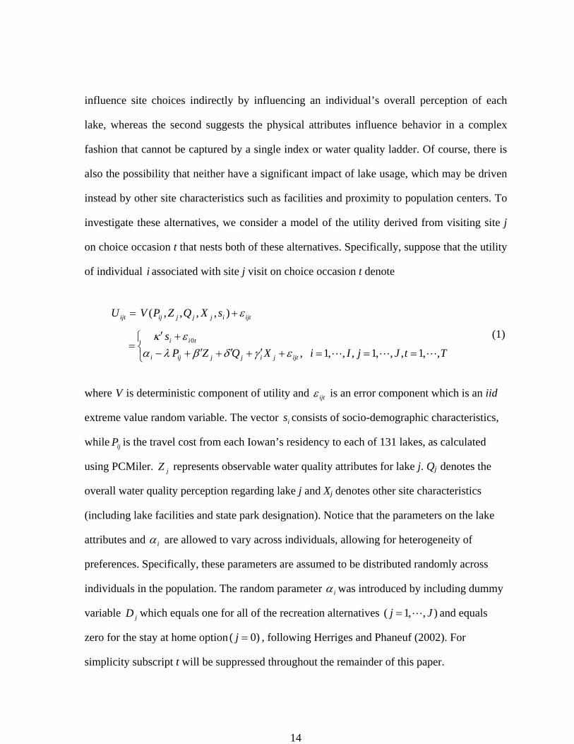
investigate these alternatives, we consider a model of the utility derived from visiting site j
on choice occasion t that nests both of these alternatives. Specifically, suppose that the utility
of individual associated with site j visit on choice occasion t denote i
⎩⎨⎧
===+′+′+′+−+′
=
+=
,,1,,,1,,,1 ,
),,,,(
0
TtJjIiXQZPs
sXQZPVU
ijtjijjiji
tii
ijtijjjijijt
εγδβλαεκ
ε
(1)
where V is deterministic component of utility and ijtε is an error component which is an iid
extreme value random variable. The vector consists of socio-demographic characteristics,
while is the travel cost from each Iowan’s residency to each of 131 lakes, as calculated
using PCMiler. represents observable water quality attributes for lake j. Qj denotes the
overall water quality perception regarding lake j and Xj denotes other site characteristics
(including lake facilities and state park designation). Notice that the parameters on the lake
attributes and
is
ijP
jZ
iα are allowed to vary across individuals, allowing for heterogeneity of
preferences. Specifically, these parameters are assumed to be distributed randomly across
individuals in the population. The random parameter iα was introduced by including dummy
variable which equals one for all of the recreation alternatives jD ),,1( Jj = and equals
zero for the stay at home option )0( =j , following Herriges and Phaneuf (2002). For
simplicity subscript t will be suppressed throughout the remainder of this paper.
14
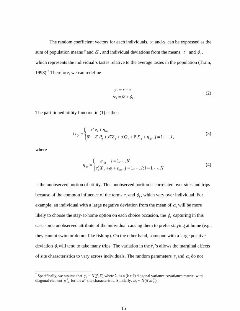
The random coefficient vectors for each individuals, ii αγ and can be expressed as the
sum of population means r and α , and individual deviations from the means, iτ and iφ ,
which represents the individual’s tastes relative to the average tastes in the population (Train,
1998).7 Therefore, we can redefine
.ii
ii rφαατγ+=+=
(2)
The partitioned utility function in (1) is then
⎩⎨⎧
=++′+′+′−+′
=,,,1,
0
JjXQZPz
Uijtjjjij
tiiijt ηγδβλα
ηκ (3)
where
(4) ⎩⎨⎧
==++′=
=NiJjX
Ni
ijtiji
tiijt ,,1;,,1,
,,1 0
εφτε
η
is the unobserved portion of utility. This unobserved portion is correlated over sites and trips
because of the common influence of the terms iτ and iφ , which vary over individual. For
example, an individual with a large negative deviation from the mean of iα will be more
likely to choose the stay-at-home option on each choice occasion, the iφ capturing in this
case some unobserved attribute of the individual causing them to prefer staying at home (e.g.,
they cannot swim or do not like fishing). On the other hand, someone with a large positive
deviation iφ will tend to take many trips. The variation in the iγ ’s allows the marginal effects
of site characteristics to vary across individuals. The random parameters iγ and iα do not
7 Specifically, we assume that ),(~ Σγγ Ni whereΣ is a (k x k) diagonal variance covariance matrix, with diagonal element for the kth site characteristic. Similarly, 2
kγσ ),(~ 2ασαα Ni .
15
vary over sites or choice occasions. Thus, the same preferences are used by the individual to
evaluate each site across time periods. Since the unobserved portion of utility is correlated
over sites and trips choice occasions the familiar IIA assumption does not apply.
Given that the ijtε ’s are assumed to be iid extreme value, the resulting model
corresponds to McFadden and Train’s (2000) mixed logit framework. A mixed logit model is
defined as the integration of the logit formula over the distribution of unobserved random
parameters (Revelt and Train, 1998). Let the vector of random parameters in the model
defined above denoted by ),( iii γαω = and let ),,,,( κλγδβξ = denote the fixed parameters.
If the random parameters, iω , were known then the probability of observing individual
choosing alternative on choice occasion t would follow the standard logit form i j
.)],(exp[
)],(exp[),(
0∑=
= J
kiikt
iijtiijt
V
VL
ξω
ξωξω (5)
Since the iω are unknown, the corresponding unconditional probability, ),( ξθijtP is obtained
by integrating over an assumed probability density function for the iω ’s. The unconditional
probability is now a function of θ , where θ represents the estimated moments of the random
parameters.8 This repeated Mixed Logit model assumes the random parameters are iid
distributed over the individuals with
∫= ωθωξωξθ dfLP iiijtijt )|(),(),( . (6)
8 In the current model, ),,,,,( 1 ασσσαγθ rkr=
16
No closed form solution exists for this unconditional probability and therefore simulation is
required for the maximum likelihood estimates of θ .9
Two hypotheses are of interest. The first hypothesis of interest is , i.e.,
whether or not individuals care about physical quality measures directly. The second
hypothesis of interest is ; i.e., whether or not the perceptions regarding water
quality at the lake, based on USEPA’s water quality ladder, directly influence individual
household behavior. Egan (2003)'s model is the restricted one based on the hypothesis
; i.e., assuming that the physical water quality measures directly influence
household behavior but water quality perceptions do not. Adamowicz et al. (1997) compared
two restricted models and estimated WTPs: one is the model under the hypothesis 1 (using
perceptual data only) and the other one is under hypothesis 2 (using physical quality data
only). The advantage of the current work is that we have a much more extensive list of
physical water quality measures and perceptions data for a larger set of site alternatives.
10 :H β = 0
0
20 :H δ =
0:20 =δH
One issue in using the water quality perceptions data in modeling site choice is that
we do not have data on this water quality perception for each individual and lake
combination. This is similar to the problem associated with catch rate data in standard
recreation demand models; i.e., because a household only visits a limited number of lakes,
individual catch rate information is typically only available for these visited lakes. Moreover,
the catch rates information itself is endogenous. Following the standard procedure used in
case of catch rate, the mean water quality assessment of a lake is used as a proxy variable for
water quality perception in this model because some lakes have a few visitors and
respondents providing water quality assessments.
9 Train (2003) describes simulation methods for use with mixed logit models, in particular maximum simulated likelihood which we employ. Software written in GAUSS to estimate mixed logit models is available from Train’s home page at http://elsa.berkeley.edu/~train.
17
IV. Estimation Result
A. Specification
Although the model for testing the null hypothesis and welfare estimation is set in
equation (1), the functional forms to be useful for the physical water quality measures, lake
characteristics and socio-demographic variables are unknown. Economic theory provides
little or no guidance in terms of these choices. Egan et al. (2004), however, provides an
extensive investigation into the choice of functional form for water quality measures, lake
characteristics and socio-economic variables in their model of recreation. Specifically, using
data from the first year of the Iowa Lakes survey, they split the available sample into 3
subsamples, using the first for specification search, the second for estimation and the third for
investigating out-of-sample predictions. They focused on modeling the role of water quality
characteristics in determining recreation demand patterns, holding constant the manner in
which both socio-demographics and other site characteristics impact preferences. The
specification search process involved comparing numerous combinations of linear and
logarithmic forms for the water quality measures. In the analysis below, we follow Egan et
al.’s (2004) final specification for the physical measures, lake characteristics and socio-
demographic variables.
Socio-demographic characteristics are assumed to enter through the “stay-at-home”
option. They include age and household size, as well as dummy variables indicating gender
and college education. A quadratic age term is included in the model to allow for
nonlinearities in the impact of age. Site characteristic are included with random coefficients.
This is to allow for heterogeneity in individual preferences regarding site characteristics,
such as wake restrictions and site facilities. For example, some households may prefer to visit
less developed lakes with wake restrictions in place, while others are attracted to sites
18
allowing the use of motorboats, jet skis, etc. It is assumed that the random parameters iγ are
each normally distributed with the mean ( kγ ) and dispersion ( kγσ ) for each parameter.
Physical water measures ( ) are categorized into five groups 1) Secchi depth, 2)
Chlorophyll, 3) Nutrients (Total Nitrogen and Total phosphorus), 4) Suspended solids
(Inorganic and Organic) and 5) Bacteria (Cyanobacteria and Total). The first four
characteristic groups directly impact the visible features of the water quality, making it more
likely that households respond to them. Bacteria is included because surveyed households
report it to be the single most important water quality concern (Azevedo et al., 2003). Egan
et al.’s (2004) specification search results suggested bacteria, Chlorophyll, and nutrients
enter logarithmically and the remaining variables enter linearly. This model is referred to as
Model A. A more complex model, including pH, alkalinity, silicon, nitrates, and ammonium
nitrogen is referred to Model B. These additional variables are entered in a linear form,
except for pH for which is a quadratic term is also included.
jZ
A total of seven models are considered. The first four represent variations on models
A and B in Egan et al. (2004):
Model A1: Model A as estimated in Egan et al. (2004)
Model A2: A1 plus the water quality perceptions variable
Model B1: Model B as estimated in Egan et al. (2004)
Model B2: B1 plus the water quality perceptions variable.
In terms of equation (3), the difference between models A1 and A2 (B1 and B2) is that A1 (B1)
constrains 0=δ , hypothesis . We include also three models to illustrate the consequences
of relying on a single measure of water quality, in this case one that is widely used by the
U.S. Environmental Protection Agency:
20H
Model C1: Model A, but replacing all physical water quality measures
19
with the single water quality ladder index.
Model C2: Model A2, but replacing all physical water quality measures
with a single water quality ladder index.
Model C3: Model A1 with the physical water quality attributes constrained
to have no impact (i.e., 0=β in equation 3).
Note that it is the comparison of models A1 and C3 that provides the basis for testing
hypothesis . 10H
B. Estimation Result
The resulting parameter estimates are presented in two Tables, 8a and 8b. Table 8a
lists parameter estimates for socio-demographic variables and mean and dispersion
parameters for random coefficients for lake amenities data. All the coefficients are significant
at 5% level except for inorganic suspended solids for Model B1 and B2 and some of the
socio-demographic data including age, age square and school dummy variables. While age
variable for Model A1, B1, B2, and C1 are not significant, age square variable is not
significant for Model A2. School variable is not significant only for Model A1. Note that the
socio-demographic data are included in the conditional indirect utility for the stay-at-home
option. Therefore, larger households are all more likely to take a trip to a lake. Age has a
convex relationship with the stay-at-home option and therefore has a concave relationship
with trips. For Model C2 and C3, the peak occurs at about age 48, which is consistent with the
estimate of larger households taking more trips, as at this age the household is more likely to
include children. Higher-educated individuals appear to be likely to stay-at-home, with
positive coefficients. The price coefficient is negative as expected and virtually identical in
all seven models.
20
Turning to the site amenities, all of the parameters are of the expected sign. As the
size of a lake increases, has a cement boat ramp, gains handicap facilities, or is adjacent to a
state park, the average number of visits to the site increases. Notice, however, the large
dispersion estimates. For example, in Model A1 the dispersion on the size of the lake
indicates almost all people prefer bigger lakes. The large dispersion on the “wake” dummy
variable seems particularly appropriate given the potentially conflicting interests of anglers
and recreational boaters. Anglers would possibly prefer “no wake” lakes, while recreational
boaters would obviously prefer lakes that allow wakes. It seems the population is roughly
split, with 62 percent preferring a lake that allows wakes and 38 percent preferring a “no
wake” lake. Lastly, the mean of iα , the trip dummy variable, is negative, indicating that on
average the respondents receive higher utility from the stay-at-home option, which is
expected considering the average number of trips is 7 out of a possible 52 choice occasions.
The physical water qualities and mean perception coefficients are reported in Table
8b. Entering mean perception in the Model A and/or Model B does not change the
coefficients much. For four models, the effect of Secchi depth is positive, while inorganic
(volatile) suspended solid have a negative impact, indicating that respondents strongly value
water clarity. However, the coefficients on chlorophyll and volatile suspended solids are
positive, suggesting that on average respondents do not mind some “greenish” water. The
negative coefficient on total phosphorus, the most likely principal limiting nutrient,
indicating higher algae growth leads to fewer recreational trips. Total nitrogen having a
positive coefficient is consistent with expectation given the negative sign on total
phosphorus. With such large amounts of phosphorus in the water, more nitrogen can actually
be beneficial by allowing a more normal phosphorus-to-nitrogen ratio. Two other forms of
nitrogen, NO3+NO2 and NH3+NH4, are negative. Continuing with the additional measures in
21
Model B, alkalinity has a positive coefficient, consistent with alkalinity’s ability to both act
as a buffer on how much acidification the water can withstand before deteriorating and as a
source of carbon, keeping harmful phytoplankton from dominating under low CO2 stress.
Since all of the lakes in the sample are acidic (i.e., pH greater than seven), a positive
coefficient for alkalinity is expected. The positive coefficient on silicon is also consistent
since silicon is important for the growth of diatoms, which in turn are a preferred food source
for aquatic organism. pH is entered quadratically, reflecting the fact that low or high pH
levels are signs of poor water quality. However, as mentioned, in our sample of lakes all of
the pH values are normal or high. The coefficients for pH show a convex relationship (the
minimum is reached at a pH of 8.3) to trips, indicating that as the pH level rises above 8.3,
trips are predicted to increase. This is the opposite of what we expected.
The water quality perception has a positive and statistically significant impact in
model A2 and model B2. Entering mean perception in model A and B does not change the
signs or general size of the physical water quality measures. The coefficients on water quality
perceptions indicate that lakes which have higher mean perception are more likely to be
places where individuals want to visit, as we expected. Clearly we reject the hypothesis
that the physical water quality measures above capture the full impact of water quality on the
household’s trip patterns. Water quality perceptions, as captured by , also significantly
affect where people choose to recreate. However, it is also clear that the perceptions index is
also an incomplete measure of how water quality affects household behavior. We clearly
reject the restriction
20H
jQ
0=β ( ) using either models A or B. 10 10H
10 The corresponding likelihood ratio test statistics or (p-value < 0.001) for model A whereas (p-value < 0.001) for model B.
822 =χ 502 =χ
22
V. Welfare Estimation
Based on the test results in section IV and the random parameter vector estimates,
) ,( ′= iii αγθ , the conditional compensating variation associated with a change in water
quality from to for individual on choice occasion is Q Q′ i t
⎭⎬⎫
⎩⎨⎧
−′−= ∑ ∑= =
J
j
J
jiijtiijtPiit QVQVCV
0 0])];[exp(ln[])];[exp(ln[1)( θθ
βθ , (4)
which is the compensating variation for the standard logit model. The unconditional
compensating variation does not have a closed form, but it can be simulated by
∑ ∑ ∑= = = ⎭
⎬⎫
⎩⎨⎧
−′−=R
r
J
j
J
j
riijt
riijtPiit QVQV
RCV
1 0 0])];[exp(ln[])];[exp(ln[11)( θθ
βθ , (5)
where R is the number of draws and r represents a particular draw from its distribution. The
simulation process involves drawing values of ) ,( ′= iii αγθ and then calculating the resulting
compensating variation for each vector of draws, and finally averaging over the results for
many draws. Following Von Haefen (2003), 2,500 draws were used in the simulation.
Three water quality improvement scenarios, measured by water quality index and/or
water quality perception, are considered with the results from model 5 and 7 used for all the
scenarios. The first scenario improves all 130 lakes to the water quality of West Okoboji
Lake, the clearest, least impacted lake in the state. Table 9 compares the water quality
perception and water quality index of West Okoboji Lake with the average of the other 130
lakes. Two of West Okoboji Lake’s measures are considerably improved over the other 130.
Water quality index and water quality perception are second highest (90.8 and 6.81
respectively) among 130 lakes. Given such a large change, “boatable” to “swimmable” and
“swimmable” to “drinkable” according to water quality ladder, the annual compensating
23
variation estimates are $12.39 and $73.03 using model 5 and 7 respectively (Table 11) for
every Iowa household. Aggregating to the annual value for all Iowans simply involves
multiplying by the number of households in Iowa, which is 1,153,20511. Table 10 also reports
the average predicted trips before and after the water quality improvement. Improving all 130
lakes to the water quality perception of West Okoboji Lakes leads to 18 percent increase in
average trips while improving to the water quality index of West Okoboji Lakes leads to 16
percent increase in average trips.
The next scenario is a less ambitious, more realistic plan of improving nine lakes to
the water quality of West Okoboji Lake (see Table 9 for comparison). The state is divided
into nine zones with one lake in each zone, allowing every Iowan to be within a couple of
hours of a lake with superior water quality. The nine lakes are chosen based on
recommendations by the Iowa Department of Natural Resources for possible candidates of a
clean-up project. The annual compensating variation estimate is $0.90 when water quality
improvement measured by water quality index and $8.26 when quality improvement
measured by water quality perception. As expected, this estimate is 7 percent and 11 percent
of the value if all lakes were improved. This suggests location of the improved lakes is
important and, to maximize Iowan’s benefit from improving a few lakes, policymakers
should consider dispersing them through the state.
The last scenario is also a policy-oriented improvement. Currently of the 131 lakes,
65 are officially listed on the EPA’s impaired water list. TMDLs are being developed for
these lakes and by 2009 the plans must be in place to improve the water quality at these lakes
enough to remove them from the list. Therefore, in this scenario, the 65 impaired lakes would
11 Number of Iowa households as reported by Survey Sampling, Inc., 2003.
24
be improved to the median mean water quality perception and/or water quality index level of
the 66 non-impaired lakes. Table 10 compares the median values for the non-impaired lakes
to the averages of the impaired lakes. This scenario is valued considerably lower than the
first water quality improvement scenario. The estimated compensating variation per Iowa
household is $3.06 when water quality perception is used and $7.28 when water quality
perceptions used. Consistent with this, the predicted trips only increase 1.24 percent for water
quality index increase and 1.90 percent for water quality perception increase.
As discussed above, there is a big margin between compensating variations, one for
water quality perception and the other for water quality index. In terms of predicted trip
change, the impact of water quality perception is bigger than that of water quality index
(14.19, 1.73 percent point for the first two scenarios and 0.7 percent point for the last
scenario). Further, the evidence that compensating variation calculated using water quality
perception is bigger than that calculated using water quality index suggests that agent’s cost-
benefit analysis of improving water quality ignoring lake visitor’s perception could be
biased, for example, underestimate in this analysis.
VI. Conclusion
Individual's day trip data collected from Iowa Lake Survey 2003 shows that
subjective quality assessment may influence individual's site choice decision. In addition,
individuals appear to have somehow different view of objective quality measures than EPA
and/or scientist. Correlation coefficients show that this disparity becomes large between two
recreation groups; water body contact group and non-water body contact group. Repeated
mixed logit model estimation result shows that individuals site choice decision depends on
25
physical water quality, water quality index and water quality perception significantly.
Further, when water quality perception is considered along with water quality index, the sign
of water quality index is opposite. As Adamowitcz et al. (1997) the models with water
quality perception entered outperform the models without water quality perception.
26
References
Adamowicz., Wiktor, Swait, Joffre, Boxall, Peter, Louvier, Jordan., Williams,
Michale.,"Perceptions versus Objective Measures of Environmental Quality in
Combined Revealed and Stated Preference Models of Environmental Valuation,"
Journal of Environmental Economics and Management., 32, 65-84 (1997).
Azevedo, C.D., K.J. Egan, J.A. Herriges, and C.L. Kling (2003). “The Iowa Lakes Valuation
Project: Summary and Findings from Year One.” CARD report.
Dillman, D. A. (1978) Mail and Telecom Surveys: The Total Design Method, New York,
Wiley.
Dillman, D. A. (2000) Mail and Telecom Surveys: The Tailored Design Method, John Wiley
and Sons, New York.
Ditton., Robert and Thomas L. Goodale, "Water Quality Perception and the Recreational
Uses of Green Bay, Lake Michigan," Water Resources Research, Vol. 9, No. 3., June
1973.
Egan, Kevin. J (2003), "Recreation Demand using Physical Water Quality Measures,"
unpublished Ph.D. Dissertation, Iowa State University.
Egan, Kevin. J, Joseph A. Herriges, Catherine L. Kling, and John A. Downing (2004),
“Recreational Demand Using Physical Measures of Water Quality,” Working Paper
04-WP372, Center for Agricultural and Rural Development, Ames, Iowa, Octorber.
Herriges, J., and D. Phaneuf (2002). “Introducing Patterns of Correlation and Substitution in
Repeated Logit Models of Recreation Demand.” American Journal of Agricultural
Economics 84: 1076-1090.
Leggett, Christopher G. (2002) "Environmental Valuation with Imperfect Information,"
Environmental and Resource Economics, 23: 343-355, 2002.
27
McFadden and Train (2000)?
Phaneuf, D.J., C.L. Kling, and J.A. Herriges (2000). “Estimation and Welfare Calculations in
a Generalized Corner Solution Model with an Application to Recreation Demand.”
The Review of Economics and Statistics 82 (1): 83-92.
Revelt, D., and K. Train (1998). “Mixed Logit with Repeated Choices: Households’ Choices
of Appliance Efficiency Level.” The Review of Economics and Statistics 80: 647-57.
Train, K. (1998). “Recreation Demand Models with Taste Differences Over People.” Land
Economics 74 (2) (May): 230-239.
Train, K. (1999). “Mixed Logit Models for Recreation Demand”, in: C.L. Kling, J. Herriges
(Eds.), Valuing Recreation and the Environment, Edward Elgar Publishing Ltd.
Train, K. (2003). “Discrete Choice Methods with Simulation. Cambridge University Press,
Cambridge, UK.
EPA water quality inventory for the state of Iowa, 2003
McClelland, Nina I. “Water Quality Index Application in the Kansas River Basin,” EPA-
907/9-74-001, February 1974.
Carlson, Robert E. “A Trophic State Index for Lakes,” Limnology and Oceanography, Vol.
22, No. 2, March 1977, 361-369.
28
Appendix A. Figure and Tables
Figure 1. Water Quality Ladder
29
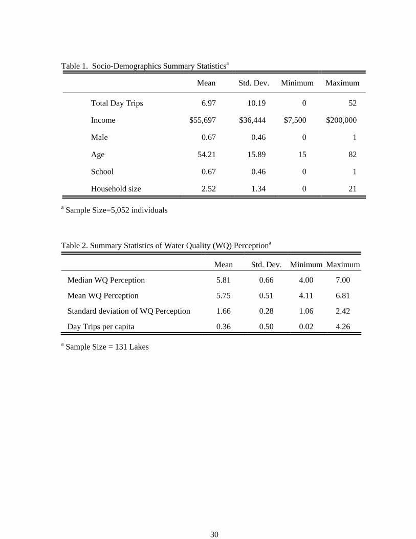
Table 1. Socio-Demographics Summary Statisticsa
Mean Std. Dev. Minimum Maximum
Total Day Trips 6.97 10.19 0 52
Income $55,697 $36,444 $7,500 $200,000
Male 0.67 0.46 0 1
Age 54.21 15.89 15 82
School 0.67 0.46 0 1
Household size 2.52 1.34 0 21
a Sample Size=5,052 individuals
Table 2. Summary Statistics of Water Quality (WQ) Perceptiona
Mean Std. Dev. Minimum Maximum
Median WQ Perception 5.81 0.66 4.00 7.00
Mean WQ Perception 5.75 0.51 4.11 6.81
Standard deviation of WQ Perception 1.66 0.28 1.06 2.42
Day Trips per capita 0.36 0.50 0.02 4.26
a Sample Size = 131 Lakes
30
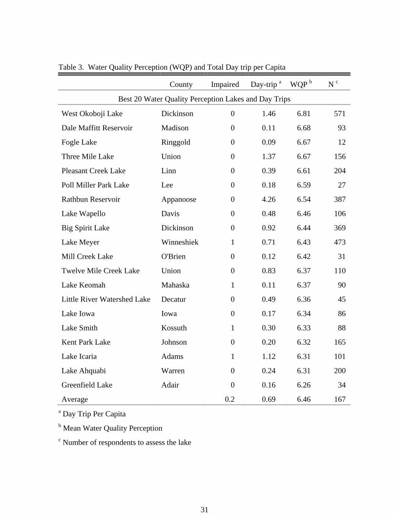
Table 3. Water Quality Perception (WQP) and Total Day trip per Capita
County Impaired Day-trip a WQP b N c
Best 20 Water Quality Perception Lakes and Day Trips
West Okoboji Lake Dickinson 0 1.46 6.81 571
Dale Maffitt Reservoir Madison 0 0.11 6.68 93
Fogle Lake Ringgold 0 0.09 6.67 12
Three Mile Lake Union 0 1.37 6.67 156
Pleasant Creek Lake Linn 0 0.39 6.61 204
Poll Miller Park Lake Lee 0 0.18 6.59 27
Rathbun Reservoir Appanoose 0 4.26 6.54 387
Lake Wapello Davis 0 0.48 6.46 106
Big Spirit Lake Dickinson 0 0.92 6.44 369
Lake Meyer Winneshiek 1 0.71 6.43 473
Mill Creek Lake O'Brien 0 0.12 6.42 31
Twelve Mile Creek Lake Union 0 0.83 6.37 110
Lake Keomah Mahaska 1 0.11 6.37 90
Little River Watershed Lake Decatur 0 0.49 6.36 45
Lake Iowa Iowa 0 0.17 6.34 86
Lake Smith Kossuth 1 0.30 6.33 88
Kent Park Lake Johnson 0 0.20 6.32 165
Lake Icaria Adams 1 1.12 6.31 101
Lake Ahquabi Warren 0 0.24 6.31 200
Greenfield Lake Adair 0 0.16 6.26 34
Average 0.2 0.69 6.46 167 a Day Trip Per Capita b Mean Water Quality Perception c Number of respondents to assess the lake
31
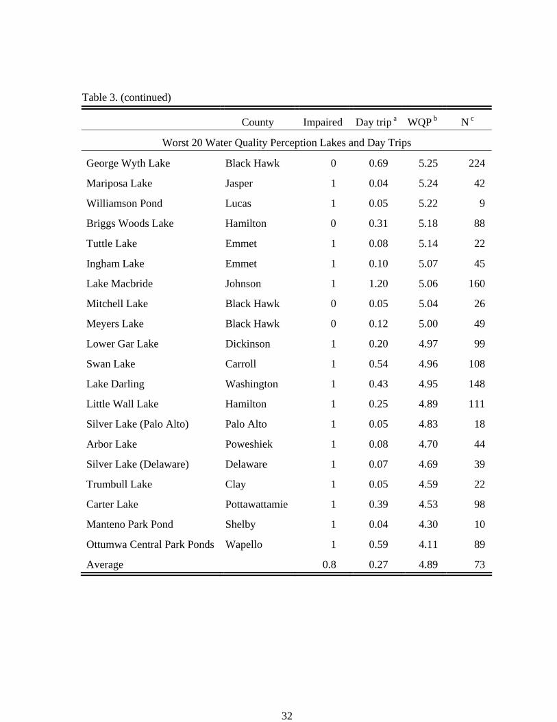
Table 3. (continued)
County Impaired Day trip a WQP b N c
Worst 20 Water Quality Perception Lakes and Day Trips
George Wyth Lake Black Hawk 0 0.69 5.25 224
Mariposa Lake Jasper 1 0.04 5.24 42
Williamson Pond Lucas 1 0.05 5.22 9
Briggs Woods Lake Hamilton 0 0.31 5.18 88
Tuttle Lake Emmet 1 0.08 5.14 22
Ingham Lake Emmet 1 0.10 5.07 45
Lake Macbride Johnson 1 1.20 5.06 160
Mitchell Lake Black Hawk 0 0.05 5.04 26
Meyers Lake Black Hawk 0 0.12 5.00 49
Lower Gar Lake Dickinson 1 0.20 4.97 99
Swan Lake Carroll 1 0.54 4.96 108
Lake Darling Washington 1 0.43 4.95 148
Little Wall Lake Hamilton 1 0.25 4.89 111
Silver Lake (Palo Alto) Palo Alto 1 0.05 4.83 18
Arbor Lake Poweshiek 1 0.08 4.70 44
Silver Lake (Delaware) Delaware 1 0.07 4.69 39
Trumbull Lake Clay 1 0.05 4.59 22
Carter Lake Pottawattamie 1 0.39 4.53 98
Manteno Park Pond Shelby 1 0.04 4.30 10
Ottumwa Central Park Ponds Wapello 1 0.59 4.11 89
Average 0.8 0.27 4.89 73
32
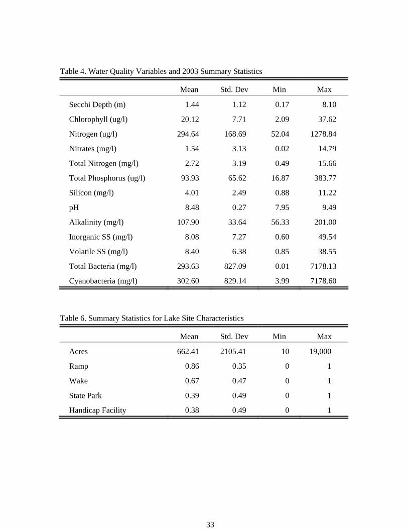
Table 4. Water Quality Variables and 2003 Summary Statistics
Mean Std. Dev Min Max
Secchi Depth (m) 1.44 1.12 0.17 8.10
Chlorophyll (ug/l) 20.12 7.71 2.09 37.62
Nitrogen (ug/l) 294.64 168.69 52.04 1278.84
Nitrates (mg/l) 1.54 3.13 0.02 14.79
Total Nitrogen (mg/l) 2.72 3.19 0.49 15.66
Total Phosphorus (ug/l) 93.93 65.62 16.87 383.77
Silicon (mg/l) 4.01 2.49 0.88 11.22
pH 8.48 0.27 7.95 9.49
Alkalinity (mg/l) 107.90 33.64 56.33 201.00
Inorganic SS (mg/l) 8.08 7.27 0.60 49.54
Volatile SS (mg/l) 8.40 6.38 0.85 38.55
Total Bacteria (mg/l) 293.63 827.09 0.01 7178.13
Cyanobacteria (mg/l) 302.60 829.14 3.99 7178.60
Table 6. Summary Statistics for Lake Site Characteristics
Mean Std. Dev Min Max
Acres 662.41 2105.41 10 19,000
Ramp 0.86 0.35 0 1
Wake 0.67 0.47 0 1
State Park 0.39 0.49 0 1
Handicap Facility 0.38 0.49 0 1
33
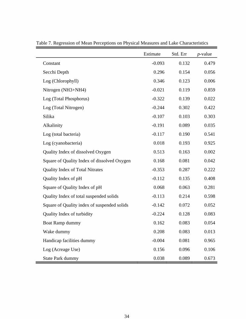
Table 7. Regression of Mean Perceptions on Physical Measures and Lake Characteristics
Estimate Std. Err p-value
Constant -0.093 0.132 0.479
Secchi Depth 0.296 0.154 0.056
Log (Chlorophyll) 0.346 0.123 0.006
Nitrogen (NH3+NH4) -0.021 0.119 0.859
Log (Total Phosphorus) -0.322 0.139 0.022
Log (Total Nitrogen) -0.244 0.302 0.422
Silika -0.107 0.103 0.303
Alkalinity -0.191 0.089 0.035
Log (total bacteria) -0.117 0.190 0.541
Log (cyanobacteria) 0.018 0.193 0.925
Quality Index of dissolved Oxygen 0.513 0.163 0.002
Square of Quality Index of dissolved Oxygen 0.168 0.081 0.042
Quality Index of Total Nitrates -0.353 0.287 0.222
Quality Index of pH -0.112 0.135 0.408
Square of Quality Index of pH 0.068 0.063 0.281
Quality Index of total suspended solids -0.113 0.214 0.598
Square of Quality index of suspended solids -0.142 0.072 0.052
Quality Index of turbidity -0.224 0.128 0.083
Boat Ramp dummy 0.162 0.083 0.054
Wake dummy 0.208 0.083 0.013
Handicap facilities dummy -0.004 0.081 0.965
Log (Acreage Use) 0.156 0.096 0.106
State Park dummy 0.038 0.089 0.673
34
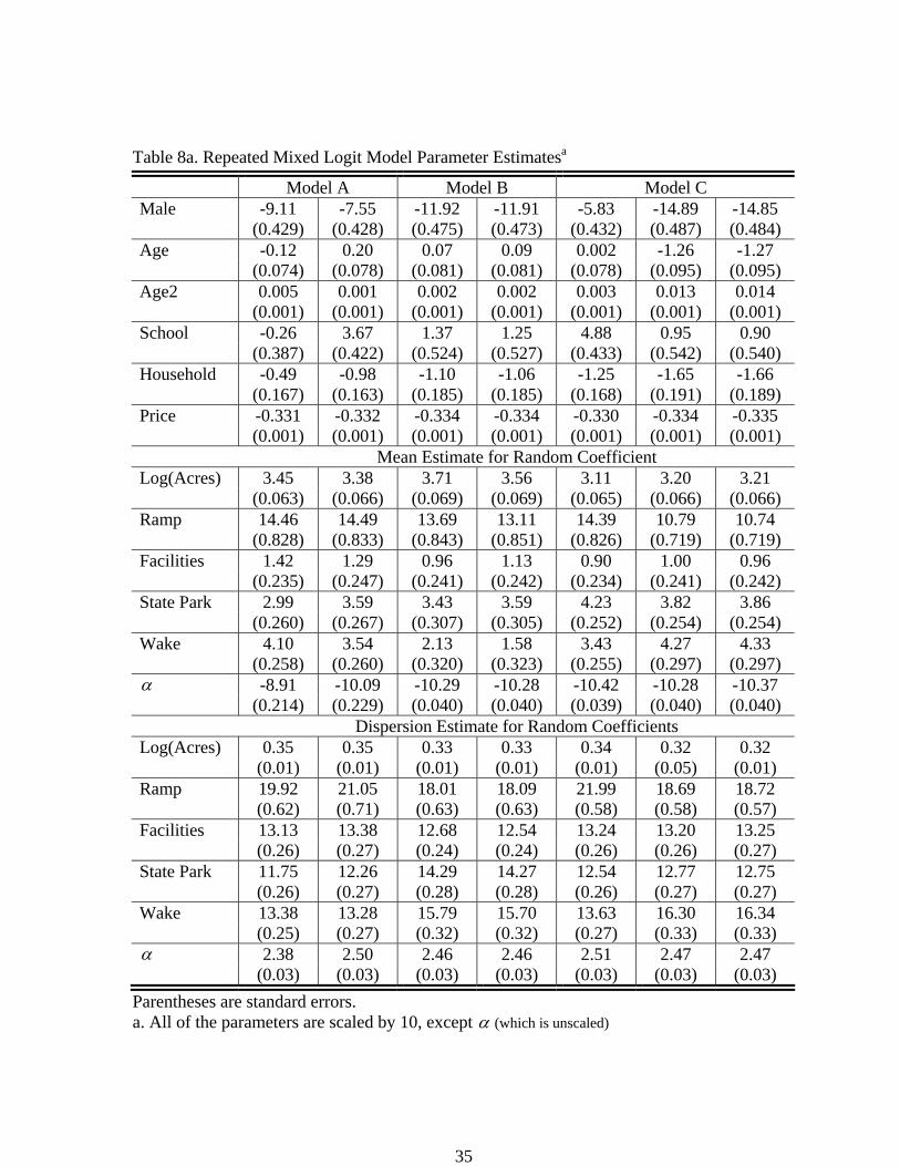
Table 8a. Repeated Mixed Logit Model Parameter Estimatesa
Model A Model B Model C Male -9.11 -7.55 -11.92 -11.91 -5.83 -14.89 -14.85 (0.429) (0.428) (0.475) (0.473) (0.432) (0.487) (0.484) Age -0.12 0.20 0.07 0.09 0.002 -1.26 -1.27 (0.074) (0.078) (0.081) (0.081) (0.078) (0.095) (0.095) Age2 0.005 0.001 0.002 0.002 0.003 0.013 0.014 (0.001) (0.001) (0.001) (0.001) (0.001) (0.001) (0.001) School -0.26 3.67 1.37 1.25 4.88 0.95 0.90 (0.387) (0.422) (0.524) (0.527) (0.433) (0.542) (0.540) Household -0.49 -0.98 -1.10 -1.06 -1.25 -1.65 -1.66 (0.167) (0.163) (0.185) (0.185) (0.168) (0.191) (0.189) Price -0.331 -0.332 -0.334 -0.334 -0.330 -0.334 -0.335 (0.001) (0.001) (0.001) (0.001) (0.001) (0.001) (0.001)
Mean Estimate for Random Coefficient Log(Acres) 3.45 3.38 3.71 3.56 3.11 3.20 3.21 (0.063) (0.066) (0.069) (0.069) (0.065) (0.066) (0.066) Ramp 14.46 14.49 13.69 13.11 14.39 10.79 10.74 (0.828) (0.833) (0.843) (0.851) (0.826) (0.719) (0.719) Facilities 1.42 1.29 0.96 1.13 0.90 1.00 0.96 (0.235) (0.247) (0.241) (0.242) (0.234) (0.241) (0.242) State Park 2.99 3.59 3.43 3.59 4.23 3.82 3.86 (0.260) (0.267) (0.307) (0.305) (0.252) (0.254) (0.254) Wake 4.10 3.54 2.13 1.58 3.43 4.27 4.33 (0.258) (0.260) (0.320) (0.323) (0.255) (0.297) (0.297) α -8.91 -10.09 -10.29 -10.28 -10.42 -10.28 -10.37 (0.214) (0.229) (0.040) (0.040) (0.039) (0.040) (0.040)
Dispersion Estimate for Random Coefficients Log(Acres) 0.35 0.35 0.33 0.33 0.34 0.32 0.32 (0.01) (0.01) (0.01) (0.01) (0.01) (0.05) (0.01) Ramp 19.92 21.05 18.01 18.09 21.99 18.69 18.72 (0.62) (0.71) (0.63) (0.63) (0.58) (0.58) (0.57) Facilities 13.13 13.38 12.68 12.54 13.24 13.20 13.25 (0.26) (0.27) (0.24) (0.24) (0.26) (0.26) (0.27) State Park 11.75 12.26 14.29 14.27 12.54 12.77 12.75 (0.26) (0.27) (0.28) (0.28) (0.26) (0.27) (0.27) Wake 13.38 13.28 15.79 15.70 13.63 16.30 16.34 (0.25) (0.27) (0.32) (0.32) (0.27) (0.33) (0.33) α 2.38 2.50 2.46 2.46 2.51 2.47 2.47 (0.03) (0.03) (0.03) (0.03) (0.03) (0.03) (0.03)
Parentheses are standard errors. a. All of the parameters are scaled by 10, except α (which is unscaled)
35
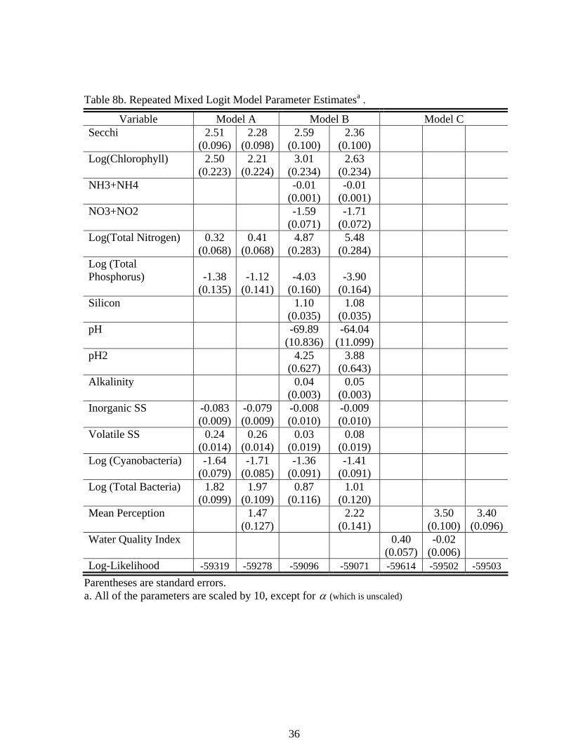
Table 8b. Repeated Mixed Logit Model Parameter Estimatesa .
Variable Model A Model B Model C Secchi 2.51 2.28 2.59 2.36 (0.096) (0.098) (0.100) (0.100) Log(Chlorophyll) 2.50 2.21 3.01 2.63 (0.223) (0.224) (0.234) (0.234) NH3+NH4 -0.01 -0.01 (0.001) (0.001) NO3+NO2 -1.59 -1.71 (0.071) (0.072) Log(Total Nitrogen) 0.32 0.41 4.87 5.48 (0.068) (0.068) (0.283) (0.284) Log (Total Phosphorus) -1.38 -1.12 -4.03 -3.90 (0.135) (0.141) (0.160) (0.164) Silicon 1.10 1.08 (0.035) (0.035) pH -69.89 -64.04 (10.836) (11.099) pH2 4.25 3.88 (0.627) (0.643) Alkalinity 0.04 0.05 (0.003) (0.003) Inorganic SS -0.083 -0.079 -0.008 -0.009 (0.009) (0.009) (0.010) (0.010) Volatile SS 0.24 0.26 0.03 0.08 (0.014) (0.014) (0.019) (0.019) Log (Cyanobacteria) -1.64 -1.71 -1.36 -1.41 (0.079) (0.085) (0.091) (0.091) Log (Total Bacteria) 1.82 1.97 0.87 1.01 (0.099) (0.109) (0.116) (0.120) Mean Perception 1.47 2.22 3.50 3.40 (0.127) (0.141) (0.100) (0.096)Water Quality Index 0.40 -0.02 (0.057) (0.006) Log-Likelihood -59319 -59278 -59096 -59071 -59614 -59502 -59503
Parentheses are standard errors. a. All of the parameters are scaled by 10, except for α (which is unscaled)
36
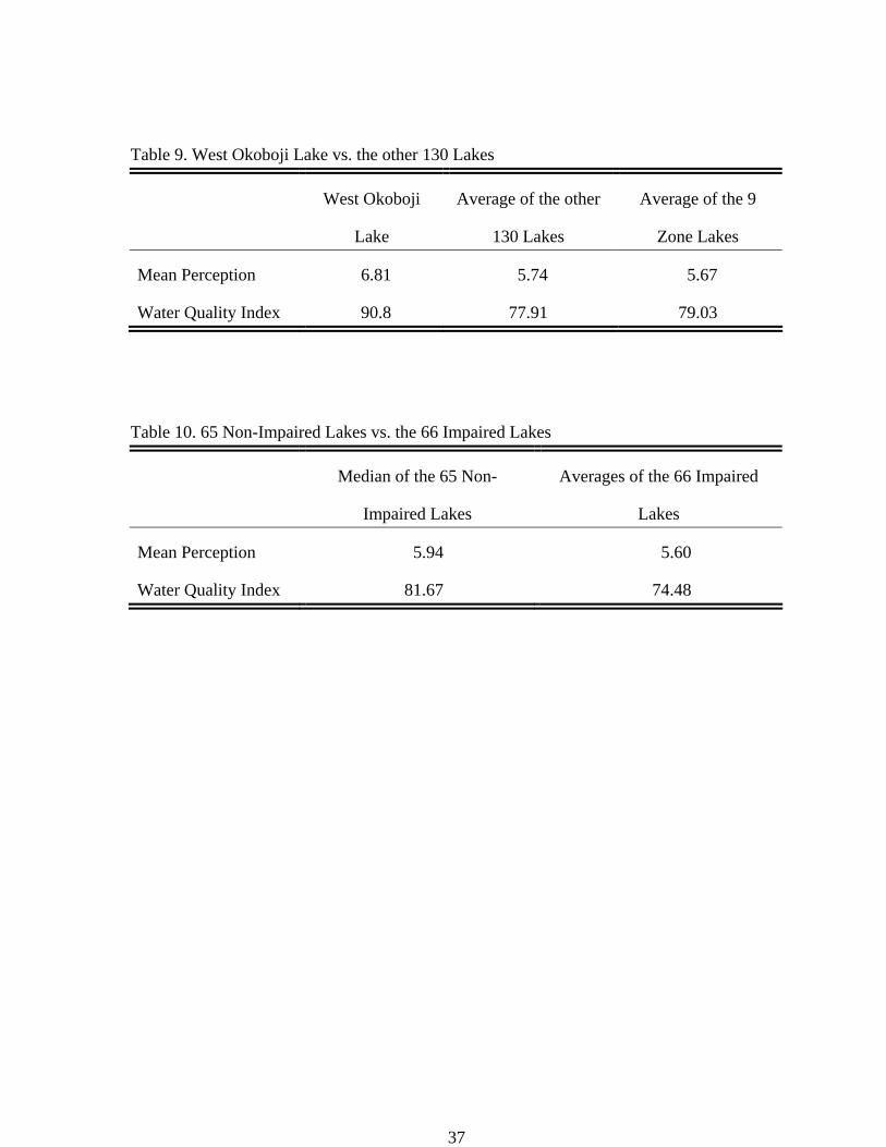
Table 9. West Okoboji Lake vs. the other 130 Lakes
West Okoboji
Lake
Average of the other
130 Lakes
Average of the 9
Zone Lakes
Mean Perception 6.81 5.74 5.67
Water Quality Index 90.8 77.91 79.03
Table 10. 65 Non-Impaired Lakes vs. the 66 Impaired Lakes
Median of the 65 Non-
Impaired Lakes
Averages of the 66 Impaired
Lakes
Mean Perception 5.94 5.60
Water Quality Index 81.67 74.48
37
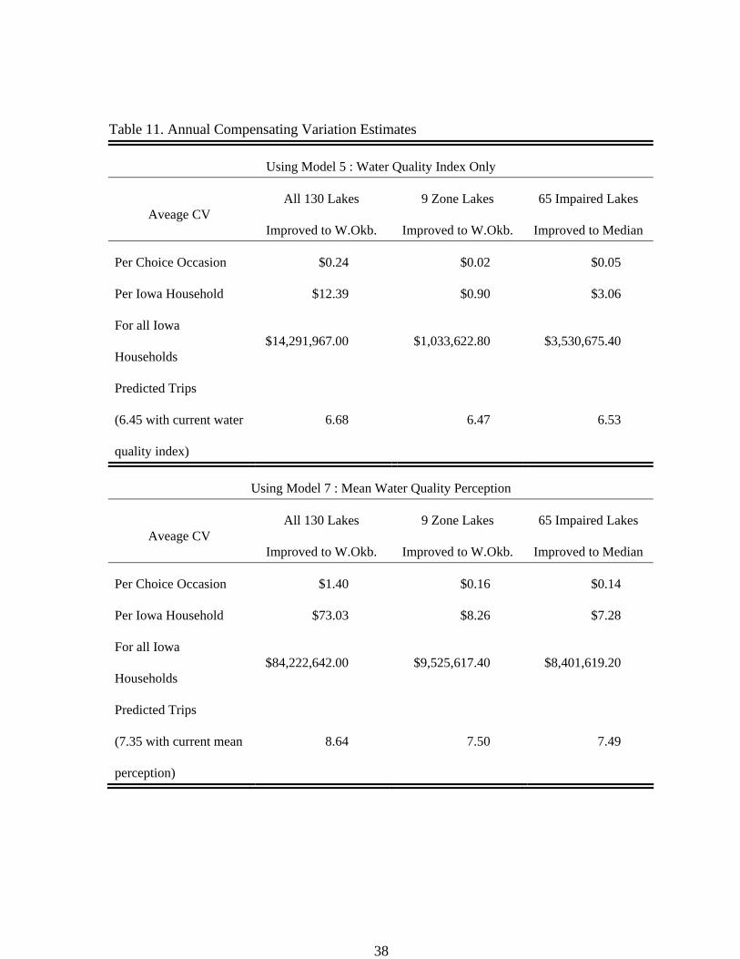
Table 11. Annual Compensating Variation Estimates
Using Model 5 : Water Quality Index Only
Aveage CV All 130 Lakes
Improved to W.Okb.
9 Zone Lakes
Improved to W.Okb.
65 Impaired Lakes
Improved to Median
Per Choice Occasion $0.24 $0.02 $0.05
Per Iowa Household $12.39 $0.90 $3.06
For all Iowa
Households $14,291,967.00 $1,033,622.80 $3,530,675.40
Predicted Trips
(6.45 with current water
quality index)
6.68 6.47 6.53
Using Model 7 : Mean Water Quality Perception
Aveage CV All 130 Lakes
Improved to W.Okb.
9 Zone Lakes
Improved to W.Okb.
65 Impaired Lakes
Improved to Median
Per Choice Occasion $1.40 $0.16 $0.14
Per Iowa Household $73.03 $8.26 $7.28
For all Iowa
Households $84,222,642.00 $9,525,617.40 $8,401,619.20
Predicted Trips
(7.35 with current mean
perception)
8.64 7.50 7.49
38
Appendix A. Water Quality Index
Water Quality Index (WQI) is a continuous scale from 0 to 100 which reflects the
composite influence of nine significant physical, chemical, and microbiological parameters
of water quality. It was developed and field evaluated by the National Sanitation Foundation
(NSF) to provide a uniform method for indicating and reporting the benefits – or lack of
benefits – realized from billions of dollars invested in stream quality improvement program.
It was developed based on an opinion research technique. A panel of 142 persons
with expertise in water quality management was carefully selected and they received a series
of mailed questionnaire. In the first questionnaire, they were asked to rate the 35 parameters
for possible inclusion in a water quality index on a scale of “1” (highest relative significance)
to “5” (lowest relative significance). In the second mailing, respondents were asked to review
their original judgments and modify them if they wished. In addition, panelists were asked to
designate not more than 15 parameters, which they considered to be the “most important” for
inclusion in a water quality index. Utilizing expert opinion derived from first two rounds of
the study, 11 parameters, or groups of parameters, were listed. In the third mailing,
respondents were asked to assign values and draw graphs for the variation in level of water
quality produced by different levels of the nine individual parameters: dissolved oxygen,
fecal coliform density, pH, biochemical oxygen demand (5-days), nitrates, phosphates,
temperature, turbidity, and total solids. Also, respondents were asked to compare relative
overall water quality, using a scale of “1” (highest relative value) to “5” (lowest relative
value) to obtain the parameter weightings. Finally, “Judgments” of all panelists were then
combined to produce a set of “average curve” scaled between 0 and 100 – one for each
parameter (see McClelland, 1974).
The WQI is derived by converting concentrations of each water quality characteristic
into a corresponding index, which is read from the quality curve. Weight for each of the
corresponding index, were derived based on the summary judgments of the expert panel.
These weights were designed to sum to 1 for the nine water quality characteristics. The
and values were combined into a composite multiplicative index of the following form:
iq
iw
iq
iw
39
∏=
n
i
wi
tq1
The subscript refers to the i-th parameter, and n is the number of parameters (in this case,
n=9). By design, WQI varies between and is bounded by 0 and 100.
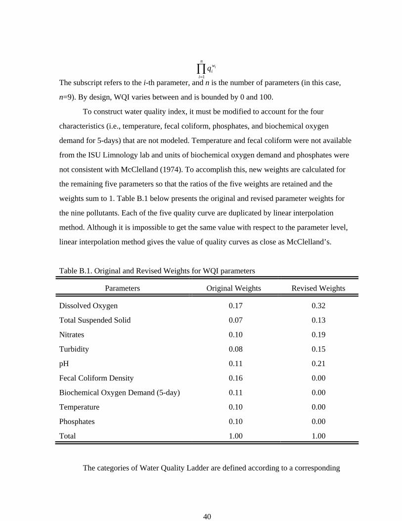
To construct water quality index, it must be modified to account for the four
characteristics (i.e., temperature, fecal coliform, phosphates, and biochemical oxygen
demand for 5-days) that are not modeled. Temperature and fecal coliform were not available
from the ISU Limnology lab and units of biochemical oxygen demand and phosphates were
not consistent with McClelland (1974). To accomplish this, new weights are calculated for
the remaining five parameters so that the ratios of the five weights are retained and the
weights sum to 1. Table B.1 below presents the original and revised parameter weights for
the nine pollutants. Each of the five quality curve are duplicated by linear interpolation
method. Although it is impossible to get the same value with respect to the parameter level,
linear interpolation method gives the value of quality curves as close as McClelland’s.
Table B.1. Original and Revised Weights for WQI parameters
Parameters Original Weights Revised Weights
Dissolved Oxygen 0.17 0.32
Total Suspended Solid 0.07 0.13
Nitrates 0.10 0.19
Turbidity 0.08 0.15
pH 0.11 0.21
Fecal Coliform Density 0.16 0.00
Biochemical Oxygen Demand (5-day) 0.11 0.00
Temperature 0.10 0.00
Phosphates 0.10 0.00
Total 1.00 1.00
The categories of Water Quality Ladder are defined according to a corresponding
40

WQI values, i.e., boatable if WQI value is 25, fishable if WQI value is 50, and swimmable if
WQI value is 70.
41
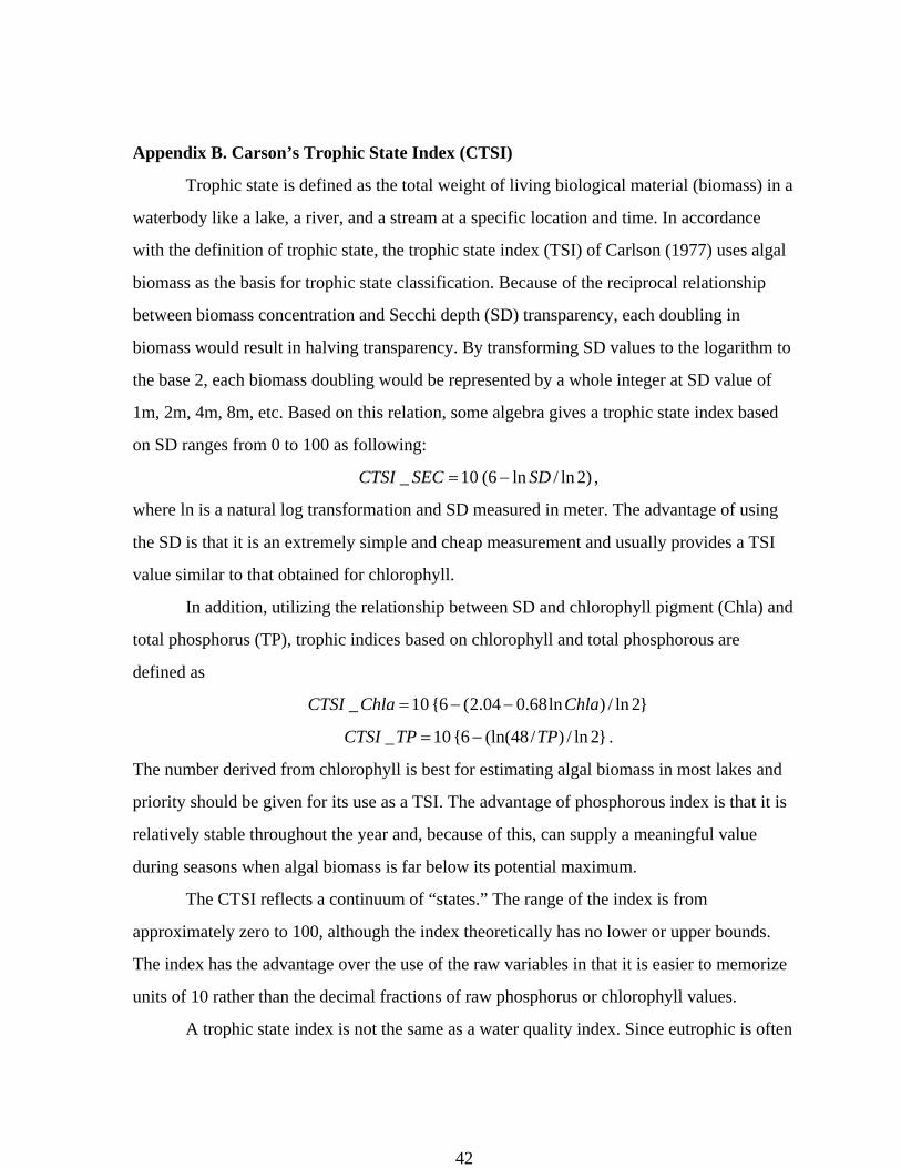
Appendix B. Carson’s Trophic State Index (CTSI)
Trophic state is defined as the total weight of living biological material (biomass) in a
waterbody like a lake, a river, and a stream at a specific location and time. In accordance
with the definition of trophic state, the trophic state index (TSI) of Carlson (1977) uses algal
biomass as the basis for trophic state classification. Because of the reciprocal relationship
between biomass concentration and Secchi depth (SD) transparency, each doubling in
biomass would result in halving transparency. By transforming SD values to the logarithm to
the base 2, each biomass doubling would be represented by a whole integer at SD value of
1m, 2m, 4m, 8m, etc. Based on this relation, some algebra gives a trophic state index based
on SD ranges from 0 to 100 as following:
)2ln/ln6(10_ SDSECCTSI −= ,
where ln is a natural log transformation and SD measured in meter. The advantage of using
the SD is that it is an extremely simple and cheap measurement and usually provides a TSI
value similar to that obtained for chlorophyll.
In addition, utilizing the relationship between SD and chlorophyll pigment (Chla) and
total phosphorus (TP), trophic indices based on chlorophyll and total phosphorous are
defined as
}2ln/)ln68.004.2(6{10_ ChlaChlaCTSI −−=
}2ln/)/48(ln(6{10_ TPTPCTSI −= .
The number derived from chlorophyll is best for estimating algal biomass in most lakes and
priority should be given for its use as a TSI. The advantage of phosphorous index is that it is
relatively stable throughout the year and, because of this, can supply a meaningful value
during seasons when algal biomass is far below its potential maximum.
The CTSI reflects a continuum of “states.” The range of the index is from
approximately zero to 100, although the index theoretically has no lower or upper bounds.
The index has the advantage over the use of the raw variables in that it is easier to memorize
units of 10 rather than the decimal fractions of raw phosphorus or chlorophyll values.
A trophic state index is not the same as a water quality index. Since eutrophic is often
42

equated with poor water quality, TSI and water quality index are confused with each other.
Water quality index depends on the use of that water and the local attitudes of the people,
which is a subjective judgment. On the other hand, the TSI is an objective standard of trophic
state of any body of water.
43