ios press m-cluster and x-ray: two methods for multi ...sxz16/papers/ica00445.pdf · multi-jammer...

Integrated Computer-Aided Engineering 21 (2014) 19–34 19DOI 10.3233/ICA-130445IOS Press

M-cluster and X-ray: Two methods formulti-jammer localization in wireless sensornetworks

Tianzhen Chenga, Ping Lia, Sencun Zhub,∗ and Don TorriericaSchool of Mechatronical Engineering, Beijing Institute of Technology, Beijing, ChinabDepartment of Computer Science and Engineering, Pennsylvania State University, University Park, PA, USAcUS Army Research Laboratory, Adelphi, MD, USA

Abstract. Jamming is one of the most severe attacks in wireless sensor networks (WSNs). While existing countermeasuresmainly focus on designing new communication mechanisms to survive under jamming, a proactive solution is to first localize thejammer(s) and then take necessary actions. Unlike the existing work that focuses on localizing a single jammer in WSNs, thiswork solves a multi-jammer localization problem, where multiple jammers launch collaborative attacks. We develop two multi-jammer localization algorithms: a multi-cluster localization (M-cluster) algorithm and an X-rayed jammed-area localization (X-ray) algorithm. Our extensive simulation results demonstrate that with one run of the algorithms, both M-cluster and X-ray areefficient in localizing multiple jammers in a wireless sensor network with small errors.

Keywords: Multi-jammer localization, wireless sensor networks, clustering, skeletonization

1. Introduction

As sensor nodes with networking capabilities be-come commercially available in recent years, wirelesssensor networks (WSNs) have been increasingly usedin industrial and civilian applications as well as inmilitary applications; e.g., industrial process monitor-ing and control, environment and habitat monitoring,traffic control, and battlefield surveillance [13]. Whensensor networks are deployed in unattended or adver-sarial environments, security becomes a major con-cern [2]. Jamming, which is one of the most serioussecurity threats in the field of WSNs, occurs when anadversary simply disregards the medium access con-trol (MAC) protocol by continually transmitting on awireless channel. The jamming is assumed to originate

∗Corresponding author: Sencun Zhu, Department of ComputerScience and Engineering, Pennsylvania State University, UniversityPark, PA 16802, USA. Tel.: +1 081 486 5995; E-mail: [email protected].

from sources embedded within the WSN or from com-promised sensors. Jamming can easily prevent normaldevices from communicating with legitimate MAC op-erations, introduce packet collisions that force repeatedbackoffs, or even jam transmissions [34]. However, it ischallenging to defend against jamming, because WSNssuffer from many constraints, including low compu-tation capability, and limited memory and energy re-sources.

To protect the communication in WSNs, many al-gorithms have been proposed to detect and defendagainst jamming, such as detection by jamming mea-surements [34], jamming evasion by channel surf-ing [35], and spread spectrum [28]. Most of these al-gorithms only detect jamming or try to keep the wire-less sensor network working under jamming. Amongthe countermeasures against jamming, determining ajammer’s location within a wireless sensor network iscritical to launching certain security actions against theadversary; e.g., deactivating the jamming device, iso-lating the jammer, or even destroying it. Only a fewworks have attempted to identify the physical locations

ISSN 1069-2509/14/$27.50 c© 2014 – IOS Press and the author(s). All rights reserved

AUTH

OR

COPY

20 T. Cheng et al. / M-cluster and X-ray: Two methods for multi-jammer localization in wireless sensor networks

of jammers in a wireless sensor network, and most ofthem [18,22,29] only focus on the scenario of a singlejammer.

A more severe jamming often involves more thanone jammer. Multiple adversaries may attack the net-work at the same time, or even one adversary mayuse multiple wireless devices to achieve a better jam-ming effect. This multi-jammer scenario would makethe existing jammer localization algorithms inapplica-ble [18,22,29]. More specifically, we define the multi-jammer scenario as collaborative jamming by multiplejammers whose jamming regions overlap. All the indi-vidually jammed areas are then merged and can be re-garded as a single jammed area. Any separate jammedarea would only be considered as the single-jammerscenario. This multi-jammer scenario raises new chal-lenges to jammer localization, as multiple jammersneed to be localized in a more complex setting.

In this work, we develop two algorithms to deal withthe multi-jammer localization problem in WSNs: amulti-cluster localization (M-cluster) algorithm and anx-rayed jammed-area localization (X-ray) algorithm.The M-cluster algorithm is based on the grouping ofjammed nodes with a clustering algorithm, and eachjammed-node group is used to estimate one jammer lo-cation. The X-ray algorithm relies on the skeletoniza-tion of a jammed area, and uses the bifurcation pointson the skeleton to localize jammers. We made a com-prehensive study of our algorithms under various con-ditions determined by node density, jammer transmis-sion power, jammer deployment, and number of jam-mers. Our simulation results show that M-cluster andX-ray can achieve a mean localization error of 6.5 me-ters and 5 meters, respectively, in the two-jammer sce-nario. Compared with the mean error of 38.5 metersin a baseline scheme, M-cluster and X-ray improve thelocalization accuracy by 80% and 86%, respectively.

The rest of the paper is organized as follows. Wereview related work in Section 2, and introduce ourmulti-jammer scenario with network and jammer mod-els in Section 3. Then we describe our algorithms inSection 4, and show the simulation results in Section 5.In Section 6, we give further discussions and talk aboutfuture work. We conclude our paper in Section 7.

2. Related work

2.1. Jamming detection

Jamming detection gives one the knowledge of thepresence of jammers in a wireless network. The exist-

ing jamming detection methods enhance network pro-tection by triggering countermeasures and providingrelevant information. In [34], Xu et al. studied four dif-ferent jamming models based on jamming behaviors(constant, deceptive, random, or reactive), and exam-ined different measurements on detecting jamming, in-cluding packet send ratio (PSR), packet delivery ra-tio (PDR), signal strength, and carrier sensing time.Cakiroglu et al. [3] proposed two algorithms for de-tecting a jamming, which are based on bad packet ra-tio (BPR), packet delivery ratio (PDR), energy con-sumption amount (ECA), and neighboring node condi-tions. Li et al. [14] proposed a sequential jamming de-tection technique that works when an increased num-ber of message collisions are observed during an obser-vation window, compared with the previously learnedlong-term average. Misra et al. [20] selected packetsdropped per terminal (PDPT) and signal-to-noise ra-tio (SNR) as the input to their fuzzy inference system.Based on the Mamdani model, the system outputs thejamming index (JI) of each node. Strasser et al. [25]suggested a method for detecting a reactive jammerthrough received signal strength (RSS) and bit errorrate (BER) sampling.

2.2. Countermeasures against jamming

Spread-spectrum (SS) physical-layer techniques us-ing direct-sequence or frequency-hopping spread spec-trum [28] are well-known countermeasures againstcommunication jamming. These solutions require thatboth the sender and the receiver share the same key andthe same pseudorandom function to generate a hoppingor spreading sequence. UFHSS [26] and UDSSS [26]deal with the problem of key establishment withoutpre-shared secret under jamming. Jamming and (unin-tentional) interference are further thwarted by the ap-plication of forward error-correcting codes and specialcoding methods [28].

For WSNs, Wood et al. [32] proposed DEEJAM, anew MAC-layer protocol for defending against stealthyjammers using IEEE 802.15.4-based hardware. Xu etal. [35] presented two techniques, called channel surf-ing and spatial retreats. The main idea is to increase theresistance to jamming by avoiding the interference asmuch as possible in either the transmission frequencydomain or the spatial domain.

Chiang and Hu [7] introduced a technique to miti-gate jamming for broadcast applications by adoptinga binary key tree to control code sequences in direct-sequence spread spectrum. Dong and Liu [9] intro-

AUTH

OR

COPY

T. Cheng et al. / M-cluster and X-ray: Two methods for multi-jammer localization in wireless sensor networks 21

duced a jamming-resistant broadcast system that orga-nizes receivers into multiple channel-sharing broadcastgroups and isolates malicious receivers using adaptivere-grouping. Jiang et al. [12] proposed a compromise-resilient anti-jamming scheme called split-pairing todeal with insider jamming in a one-hop network set-ting. Liu and Ning [17] proposed an encoding methodcalled BitTrickle to defend against broadband andhigh-power reactive jamming. Tague et al. [27] pro-posed a framework for control-channel access schemesusing the random assignment of cryptographic keysto hide the location of control channels in the pres-ence of insider jammers. Wang et al. [30] proposeda delay-bounded adaptive online UFH algorithm foranti-jamming wireless communication.

2.3. Localization against jamming devices

A few jammer-localization algorithms have beenproposed for WSNs. Pelechrinis et al. [22], based onpacket delivery ratio (PDR) and gradient descent meth-ods, designed and implemented a lightweight jammerlocalization algorithm. Their approach can find out thenearest node to the jammed area. Liu et al. devel-oped a jammer localization algorithm called VirtualForce Iterative Localization (VFIL) [16] and anotheralgorithm [18] that exploits nodes’ hearing ranges.Torrieri proposed a direction-finding and localizationmethod based on the special characteristics of spread-spectrum communications and multiple antennae [29].Cheng [6] proposed a new jammer localization al-gorithm, called Double Circle Localization (DCL).DCL uses two classic concepts in geometry, minimumbounding circle (MBC) and maximum inscribed circle(MIC), to solve the jammer localization problem. Allthese works focused on jammer localization in the con-text of a single jammer, and did not study the multi-jammer scenario in WSNs.

Recently, Liu et al. [15] tried to address the caseof two jammers coexisting in wireless networks byleveraging the network topology changes caused byjamming. They studied the jamming effects under twojammers and developed an approach to localize jam-mers under comprehensive simulations. However, theirwork does not have details about how to address thescenario with more than two jammers.

In our recent work [5], we also made a prelimi-nary study of this multi-jammer localization problemby proposing the X-ray method. In this work, we sig-nificantly extended our previous work in the follow-ing ways. First, we introduce a new technique called

M-clustering for multi-jammer localization. A com-parative study has been made for M-clustering, X-rayand a baseline scheme (as shown in Section 5). Prosand Cons of M-clustering and X-ray are also discussed(in Section 6). Second, we propose a method for jam-mer number estimation without the knowledge of jam-mer transmission range (in Section 3.3). Further, weshow through simulation that our algorithms can toler-ate well the errors caused by false estimation of jam-mer number.

3. The case of multiple jammers in wireless sensorsetworks

3.1. Effects of multiple jammers

Jamming is defined as the act of intentionally di-recting electromagnetic energy towards a communi-cation system to disrupt or prevent signal transmis-sion [21]. Wireless devices can successfully receiveinformation based on the signal-to-noise ratio (SNR)(SNR = Psignal/Pnoise), where P is the average power.Noise represents the undesirable electromagnetic spec-trum collected by antennas including the electromag-netic energy from jamming. If the SNR of a receivedmessage is below a minimum SNR threshold, the mes-sage cannot be correctly extracted and decoded fromradio signals. Accordingly, the receiver is consideredto be jammed.

The multi-jammer scenario can be described as fol-lows. Multiple jammers perform collaborative jam-ming in WSNs, and they have overlapping jammedareas. We do not consider the scenarios of a sin-gle jammer or multiple jammers with non-overlappingjammed areas. Indeed, these latter two scenarios canbe simply solved by an existing single-jammer local-ization algorithm [16,18].

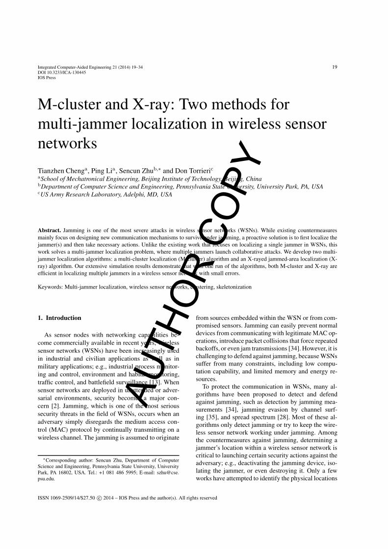
Compared with a single-jammer strategy, a multi-jammer strategy has several advantages to an adver-sary. First and the foremost, under the same overallbudget of power, the multi-jammer strategy is morepower-efficient than the single-jammer strategy be-cause of the rapid attenuation of jamming signals. InFig. 1, we compare the size of jammed areas in fourstrategies under the same overall power: one, two,three and five jammers. For simplicity, the jammedarea in a multi-jammer strategy is the sum of jammedareas caused by all the jammers. As the overall poweris fixed, if more jammers are used, each jammer will beassigned less power (1/n of the overall power, where

AUTH

OR

COPY


Fig. 1. Jammed area comparison of the single-jammer and multi-jammer strategies. X axis represents the overall jamming powerused by the jammer strategies. Jammers in one strategy share out theoverall jamming power.

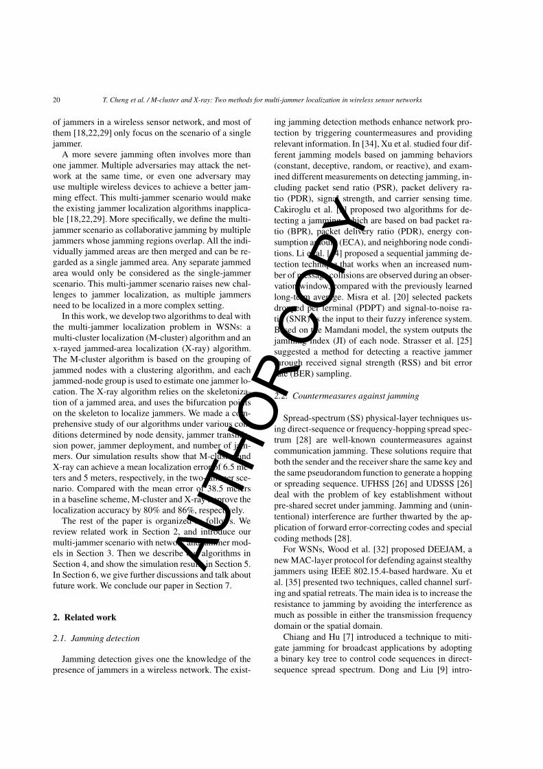
Fig. 2. An illustration of three jammers with overlapping jammingregion in the wireless sensor network.

n is the number of jammers). Figure 1 shows that, un-der the same overall power budget, more jammers re-sult in a larger jammed area (i.e., a better jammingeffect). However, from the perspective of a defender,more jammers mean more jamming-attack strategies,and hence more challenges to protect communicationand to localize jammers.

We further show a possible topology in a multi-jammer scenario. In Fig. 2, according to their connec-tivity, sensor nodes in the network are divided intothree categories: (a) jammed node, which has no com-munication with its neighbor nodes; (b) unaffectednode, whose connectivity has not been affected byjamming; (c) boundary node, whose neighbor nodes

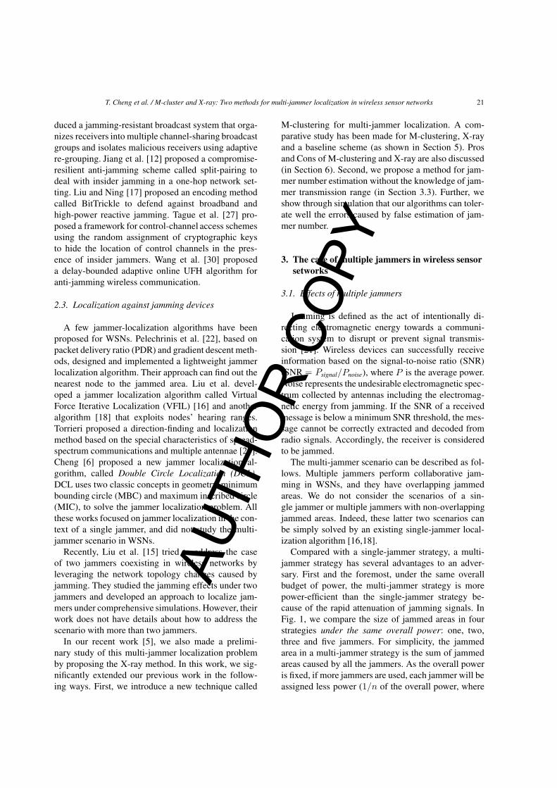
Fig. 3. An overview of the network entities and their roles in ouralgorithms.

are partially jammed. These nodes are represented inblack, white and grey dots, respectively. We note that,in the region where two jammed areas meet, the elec-tromagnetic environment is very complex. In our work,we use the sum of received signal strength of all jam-ming signals as the jamming power at each node.Therefore, as the powers of the different jamming sig-nals accumulate, some nodes near to the intersectionareas of jammed regions also become jammed.

3.2. Network and multi-jammer models withassumptions

Network model. In this paper, we first assume thatWSNs are randomly deployed and static, and a basestation is deployed to gather information and runs ourmulti-jammer localization algorithms. Nodes are as-sumed to know their own locations and can detect jam-ming. Some existing techniques might be used to pro-vide such information [19,34]. Also, every node main-tains a neighbor list and has such information as theirlocations and activeness (jammed or not). By period-ically broadcasting a beacon message, this list can beeasily obtained, and any change of the status of neigh-bors will be updated. In Fig. 3, we show the differenttypes of entities and their roles in the network at thetime of jamming.

Radio propagation channel model. In our work, we usethe radio propagation channel model in which the ratioof received to transmitted power in dB is given by

Pr

PtdB = 10 log10K − 10γ log10

d

d0− ψdB, (1)

where ψdB is a zero-mean Gaussian-distributed ran-dom variable that models the shadowing, K is a unit-less constant that depends on the antenna characteris-tics and the average channel attenuation, d0 is a refer-

AUTH

OR

COPY


ence distance for the far-field antenna, γ is the power-law attenuation or path-loss exponent, and fading is ne-glected [10,28]. In the simulations, the shadowing isneglected by setting ψdB = 0 dB, but both shadow-ing and fading will be considered in future work. Thepower-law attenuation is γ = 3.71, and K = 31.54.The radio transmission is assumed to be omnidirec-tional.

Multi-jammer model. Multiple jammers work togetherand transmit either the same or different jammingpower levels. All jammers are deployed with their loca-tions fixed. To model the deployment of multiple jam-mers in WSNs, we impose a constraint from the ad-versary’s viewpoint. Assume there are n jammers ina wireless sensor network, the distance Dij betweenjammer i and its nearest-neighbor jammer j should fol-low this condition:

Dij ∈ [ω(Ri +Rj), (Ri +Rj)], (2)

where Ri and Rj are the transmission ranges of jam-mer i and jammer j, respectively. ω ∈ (0, 1) is a vari-able. In general, a smaller ω implies closer distance be-tween two nodes. Unless specified, ω is set to 0.5 inthis work, and we will study how this parameter affectsperformance in our simulation section. Under this con-dition, jamming regions are merged, and the jammingimpact is optimized. Note that although multiple jam-mers can be deployed very closely to one another (i.e.,with a small ω), such deployments would waste the po-tential ability to jam more nodes. Moreover, when de-ploying multiple jammers very closely, localizing oneof them would be more likely to expose the other onesthat are close. Indeed, the jammers that are overly closecan be treated as a single jammer. Jammers withoutoverlapping jammed areas (i.e.,ω = 1) will be not con-sidered in this paper, as each of them can be localizedindividually as a single jammer [16,18].

3.3. Jammer number determination

In this paper, we will mainly focus on determiningthe locations of multiple jammers at one time with thenumber of jammers already known. How to accuratelydetect the number of jammers in WSNs in our multi-jammer scenario could be an interesting but undecid-able problem as jammers can vary their transmissionpowers. As such, we address this problem with heuris-tic approaches under different knowledge assumptions.We will also show the impact of false number estima-tions in the simulation section.

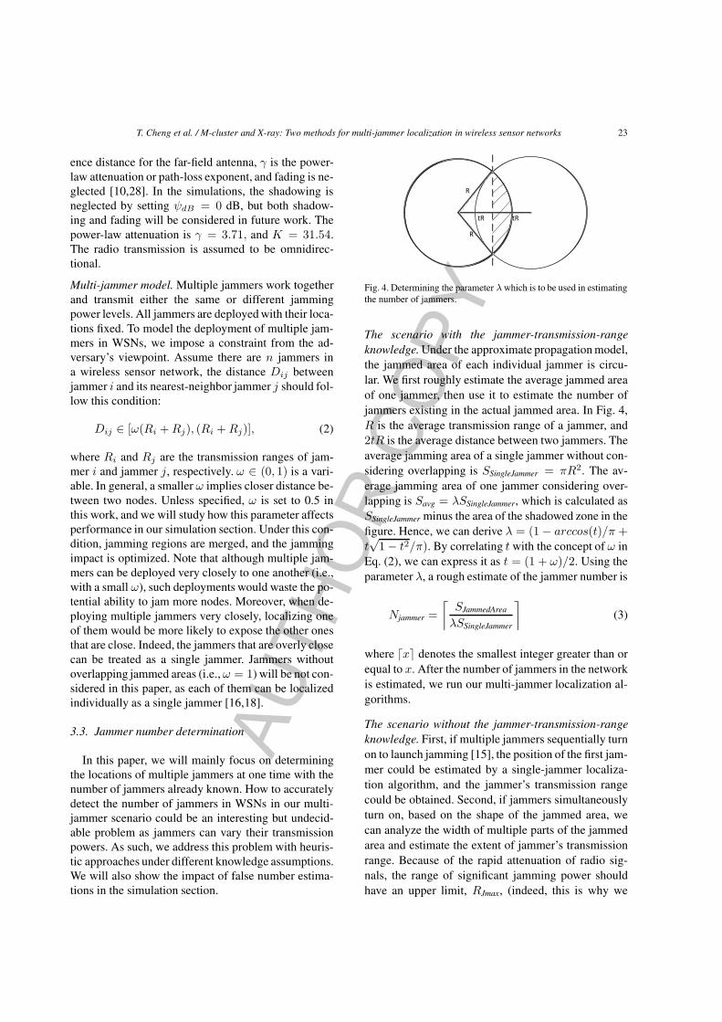
Fig. 4. Determining the parameter λ which is to be used in estimatingthe number of jammers.

The scenario with the jammer-transmission-rangeknowledge. Under the approximate propagation model,the jammed area of each individual jammer is circu-lar. We first roughly estimate the average jammed areaof one jammer, then use it to estimate the number ofjammers existing in the actual jammed area. In Fig. 4,R is the average transmission range of a jammer, and2tR is the average distance between two jammers. Theaverage jamming area of a single jammer without con-sidering overlapping is SSingleJammer = πR2. The av-erage jamming area of one jammer considering over-lapping is Savg = λSSingleJammer, which is calculated asSSingleJammer minus the area of the shadowed zone in thefigure. Hence, we can derive λ = (1− arccos(t)/π +

t√1− t2/π). By correlating t with the concept of ω in

Eq. (2), we can express it as t = (1 + ω)/2. Using theparameter λ, a rough estimate of the jammer number is

Njammer =

⌈SJammedArea

λSSingleJammer

⌉(3)

where �x� denotes the smallest integer greater than orequal to x. After the number of jammers in the networkis estimated, we run our multi-jammer localization al-gorithms.

The scenario without the jammer-transmission-rangeknowledge. First, if multiple jammers sequentially turnon to launch jamming [15], the position of the first jam-mer could be estimated by a single-jammer localiza-tion algorithm, and the jammer’s transmission rangecould be obtained. Second, if jammers simultaneouslyturn on, based on the shape of the jammed area, wecan analyze the width of multiple parts of the jammedarea and estimate the extent of jammer’s transmissionrange. Because of the rapid attenuation of radio sig-nals, the range of significant jamming power shouldhave an upper limit, RJmax, (indeed, this is why we

AUTH

OR

COPY


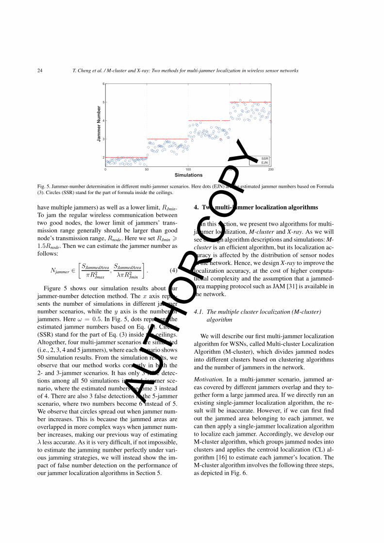
Fig. 5. Jammer-number determination in different multi-jammer scenarios. Here dots (EJN) are the estimated jammer numbers based on Formula(3). Circles (SSR) stand for the part of formula inside the ceilings.

have multiple jammers) as well as a lower limit, RJmin.To jam the regular wireless communication betweentwo good nodes, the lower limit of jammers’ trans-mission range generally should be larger than goodnode’s transmission range, Rnode. Here we set RJmin �1.5Rnode. Then we can estimate the jammer number asfollows:

Njammer ∈[SJammedArea

πR2Jmax

,SJammedArea

λπR2Jmin

]. (4)

Figure 5 shows our simulation results about ourjammer-number detection method. The x axis repre-sents the number of simulations in different jammernumber scenarios, while the y axis is the number ofjammers. Here ω = 0.5. In Fig. 5, dots represent theestimated jammer numbers based on Eq. (3). Circles(SSR) stand for the part of Eq. (3) inside the ceilings.Altogether, four multi-jammer scenarios are simulated(i.e., 2, 3, 4 and 5 jammers), where each scenario shows50 simulation results. From the simulation results, weobserve that our method works correctly in both the2- and 3-jammer scenarios. It has only 3 false detec-tions among all 50 simulations in the 4-jammer sce-nario, where the estimated numbers become 3 insteadof 4. There are also 3 false detections in the 5-jammerscenario, where two numbers become 6 instead of 5.We observe that circles spread out when jammer num-ber increases. This is because the jammed areas areoverlapped in more complex ways when jammer num-ber increases, making our previous way of estimatingλ less accurate. As it is very difficult, if not impossible,to estimate the jamming number perfectly under vari-ous jamming strategies, we will instead show the im-pact of false number detection on the performance ofour jammer localization algorithms in Section 5.

4. Two multi-jammer localization algorithms

In this section, we present two algorithms for multi-jammer localization, M-cluster and X-ray. As we willsee through algorithm descriptions and simulations: M-cluster is an efficient algorithm, but its localization ac-curacy is affected by the distribution of sensor nodesin the network. Hence, we design X-ray to improve thelocalization accuracy, at the cost of higher computa-tional complexity and the assumption that a jammed-area mapping protocol such as JAM [31] is available inthe network.

4.1. The multiple cluster localization (M-cluster)algorithm

We will describe our first multi-jammer localizationalgorithm for WSNs, called Multi-cluster LocalizationAlgorithm (M-cluster), which divides jammed nodesinto different clusters based on clustering algorithmsand the number of jammers in the network.

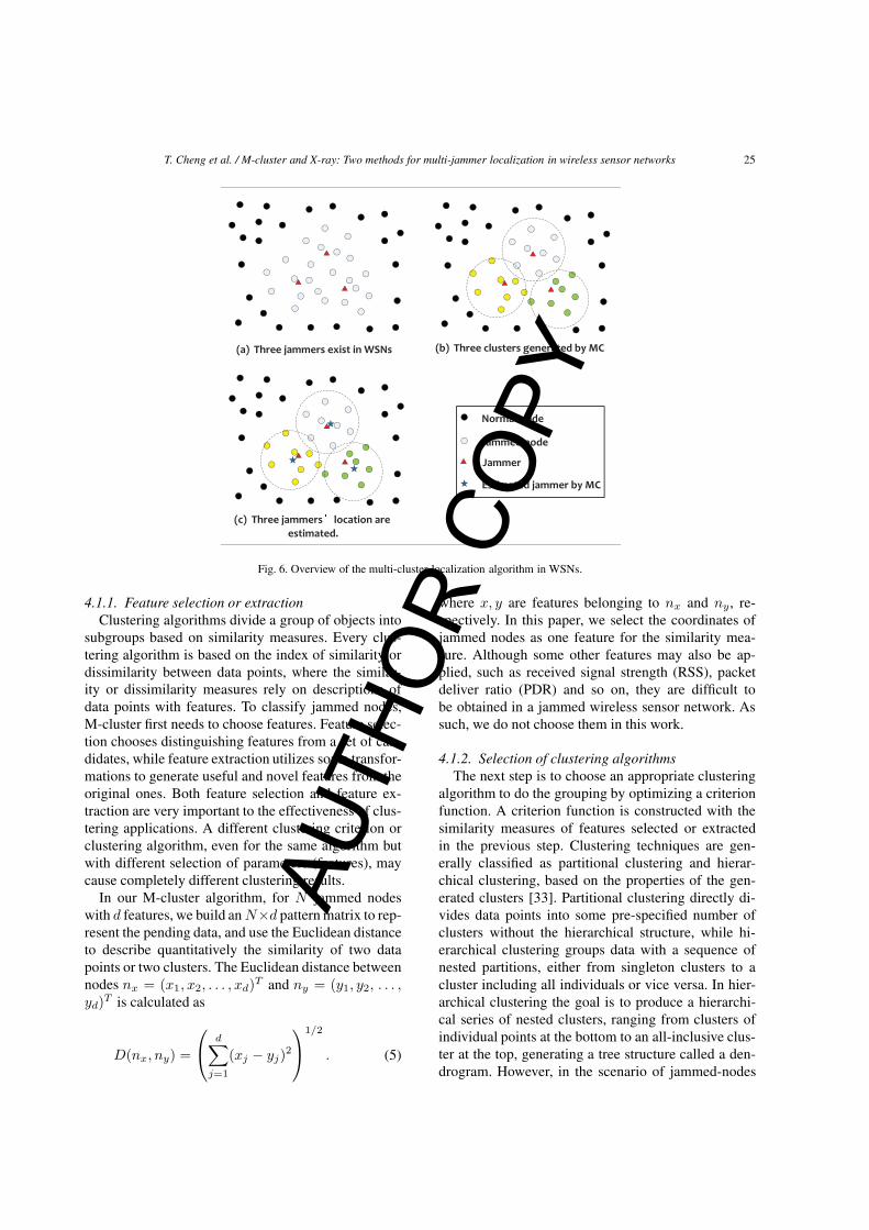
Motivation. In a multi-jammer scenario, jammed ar-eas covered by different jammers overlap and they to-gether form a large jammed area. If we directly run anexisting single-jammer localization algorithm, the re-sult will be inaccurate. However, if we can first findout the jammed area belonging to each jammer, wecan then apply a single-jammer localization algorithmto localize each jammer. Accordingly, we develop ourM-cluster algorithm, which groups jammed nodes intoclusters and applies the centroid localization (CL) al-gorithm [16] to estimate each jammer’s location. TheM-cluster algorithm involves the following three steps,as depicted in Fig. 6.

AUTH

OR

COPY


Fig. 6. Overview of the multi-cluster localization algorithm in WSNs.

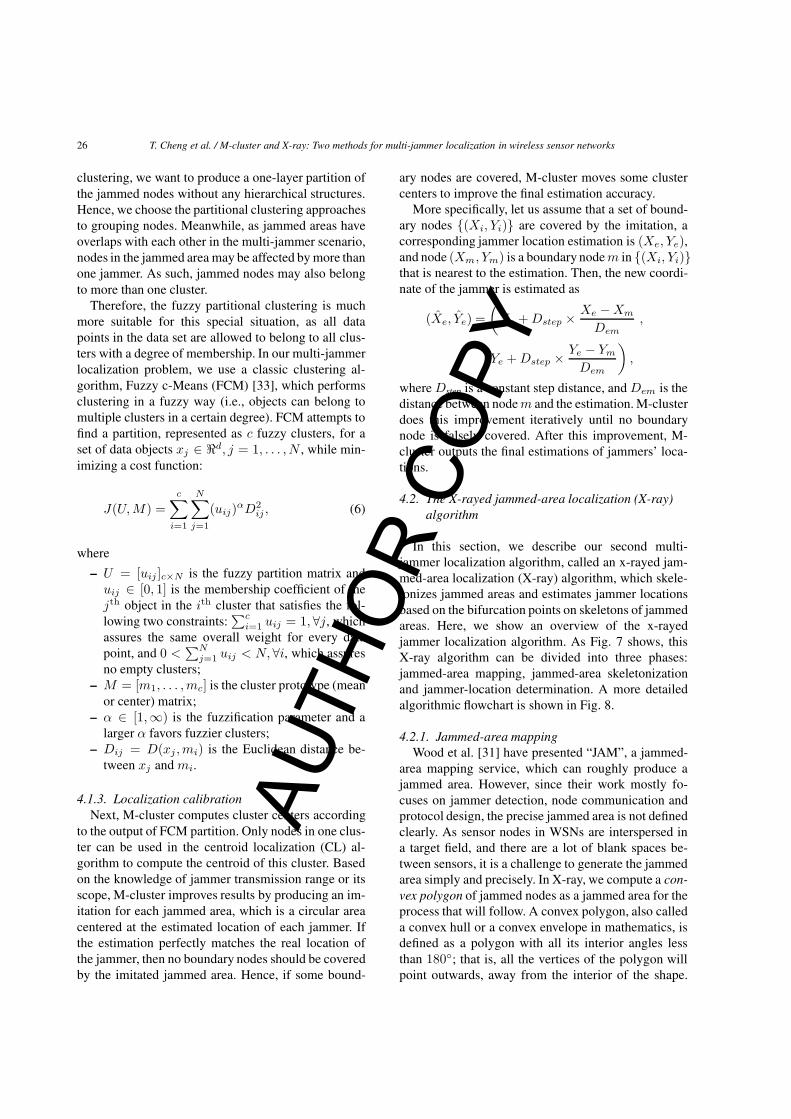
4.1.1. Feature selection or extractionClustering algorithms divide a group of objects into

subgroups based on similarity measures. Every clus-tering algorithm is based on the index of similarity ordissimilarity between data points, where the similar-ity or dissimilarity measures rely on descriptions ofdata points with features. To classify jammed nodes,M-cluster first needs to choose features. Feature selec-tion chooses distinguishing features from a set of can-didates, while feature extraction utilizes some transfor-mations to generate useful and novel features from theoriginal ones. Both feature selection and feature ex-traction are very important to the effectiveness of clus-tering applications. A different clustering criterion orclustering algorithm, even for the same algorithm butwith different selection of parameters (features), maycause completely different clustering results.

In our M-cluster algorithm, for N jammed nodeswith d features, we build anN×d pattern matrix to rep-resent the pending data, and use the Euclidean distanceto describe quantitatively the similarity of two datapoints or two clusters. The Euclidean distance betweennodes nx = (x1, x2, . . . , xd)

T and ny = (y1, y2, . . . ,yd)

T is calculated as

D(nx, ny) =

⎛⎝ d∑

j=1

(xj − yj)2

⎞⎠

1/2

. (5)

where x, y are features belonging to nx and ny, re-spectively. In this paper, we select the coordinates ofjammed nodes as one feature for the similarity mea-sure. Although some other features may also be ap-plied, such as received signal strength (RSS), packetdeliver ratio (PDR) and so on, they are difficult tobe obtained in a jammed wireless sensor network. Assuch, we do not choose them in this work.

4.1.2. Selection of clustering algorithmsThe next step is to choose an appropriate clustering

algorithm to do the grouping by optimizing a criterionfunction. A criterion function is constructed with thesimilarity measures of features selected or extractedin the previous step. Clustering techniques are gen-erally classified as partitional clustering and hierar-chical clustering, based on the properties of the gen-erated clusters [33]. Partitional clustering directly di-vides data points into some pre-specified number ofclusters without the hierarchical structure, while hi-erarchical clustering groups data with a sequence ofnested partitions, either from singleton clusters to acluster including all individuals or vice versa. In hier-archical clustering the goal is to produce a hierarchi-cal series of nested clusters, ranging from clusters ofindividual points at the bottom to an all-inclusive clus-ter at the top, generating a tree structure called a den-drogram. However, in the scenario of jammed-nodes

AUTH

OR

COPY


clustering, we want to produce a one-layer partition ofthe jammed nodes without any hierarchical structures.Hence, we choose the partitional clustering approachesto grouping nodes. Meanwhile, as jammed areas haveoverlaps with each other in the multi-jammer scenario,nodes in the jammed area may be affected by more thanone jammer. As such, jammed nodes may also belongto more than one cluster.

Therefore, the fuzzy partitional clustering is muchmore suitable for this special situation, as all datapoints in the data set are allowed to belong to all clus-ters with a degree of membership. In our multi-jammerlocalization problem, we use a classic clustering al-gorithm, Fuzzy c-Means (FCM) [33], which performsclustering in a fuzzy way (i.e., objects can belong tomultiple clusters in a certain degree). FCM attempts tofind a partition, represented as c fuzzy clusters, for aset of data objects xj ∈ �d, j = 1, . . . , N , while min-imizing a cost function:

J(U,M) =

c∑i=1

N∑j=1

(uij)αD2

ij , (6)

where

– U = [uij ]c×N is the fuzzy partition matrix anduij ∈ [0, 1] is the membership coefficient of thejth object in the ith cluster that satisfies the fol-lowing two constraints:

∑ci=1 uij = 1, ∀j, which

assures the same overall weight for every datapoint, and 0 <

∑Nj=1 uij < N, ∀i, which assures

no empty clusters;– M = [m1, . . . ,mc] is the cluster prototype (mean

or center) matrix;– α ∈ [1,∞) is the fuzzification parameter and a

larger α favors fuzzier clusters;– Dij = D(xj ,mi) is the Euclidean distance be-

tween xj and mi.

4.1.3. Localization calibrationNext, M-cluster computes cluster centers according

to the output of FCM partition. Only nodes in one clus-ter can be used in the centroid localization (CL) al-gorithm to compute the centroid of this cluster. Basedon the knowledge of jammer transmission range or itsscope, M-cluster improves results by producing an im-itation for each jammed area, which is a circular areacentered at the estimated location of each jammer. Ifthe estimation perfectly matches the real location ofthe jammer, then no boundary nodes should be coveredby the imitated jammed area. Hence, if some bound-

ary nodes are covered, M-cluster moves some clustercenters to improve the final estimation accuracy.

More specifically, let us assume that a set of bound-ary nodes {(Xi, Yi)} are covered by the imitation, acorresponding jammer location estimation is (Xe, Ye),and node (Xm, Ym) is a boundary nodem in {(Xi, Yi)}that is nearest to the estimation. Then, the new coordi-nate of the jammer is estimated as

(Xe, Ye) =

(Xe +Dstep × Xe −Xm

Dem,

Ye +Dstep × Ye − YmDem

),

where Dstep is a constant step distance, and Dem is thedistance between nodem and the estimation. M-clusterdoes this improvement iteratively until no boundarynode is falsely covered. After this improvement, M-cluster outputs the final estimations of jammers’ loca-tions.

4.2. The X-rayed jammed-area localization (X-ray)algorithm

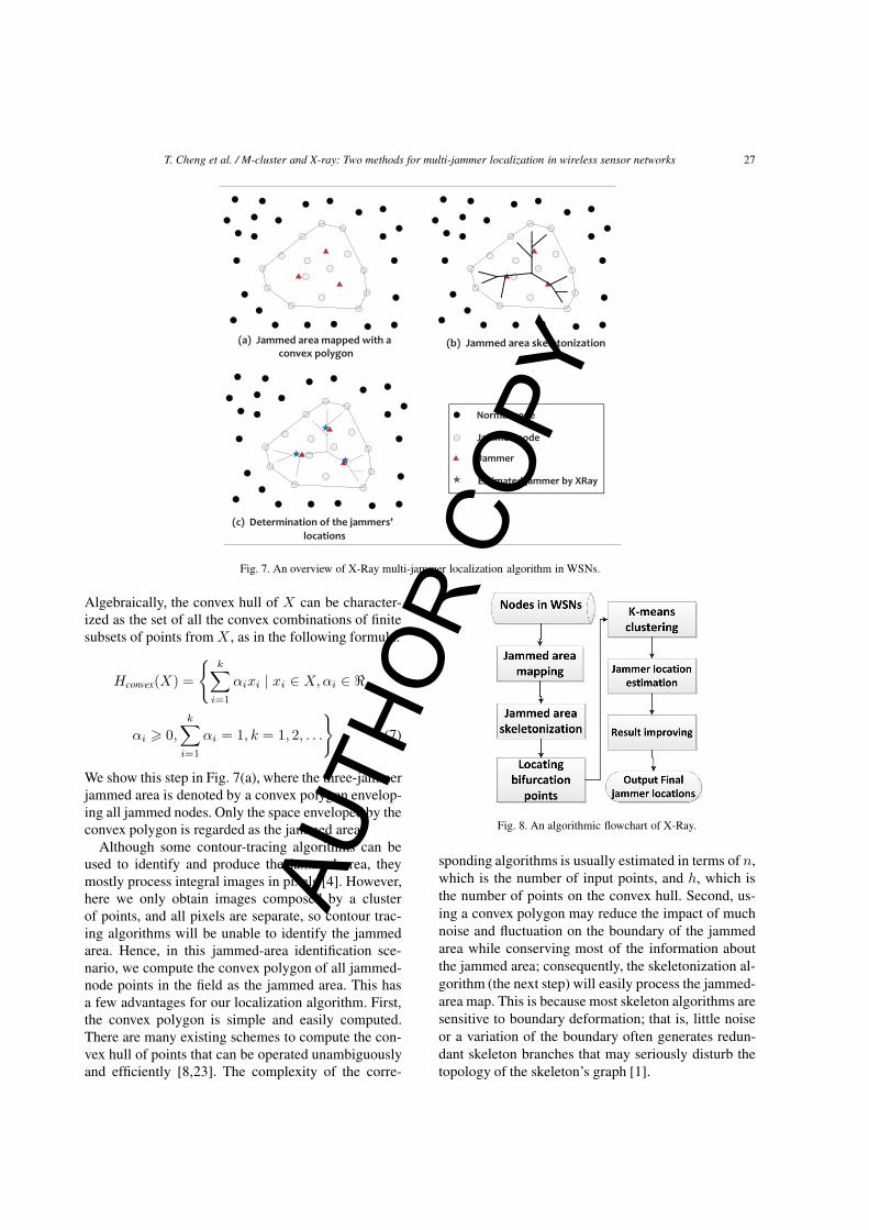
In this section, we describe our second multi-jammer localization algorithm, called an x-rayed jam-med-area localization (X-ray) algorithm, which skele-tonizes jammed areas and estimates jammer locationsbased on the bifurcation points on skeletons of jammedareas. Here, we show an overview of the x-rayedjammer localization algorithm. As Fig. 7 shows, thisX-ray algorithm can be divided into three phases:jammed-area mapping, jammed-area skeletonizationand jammer-location determination. A more detailedalgorithmic flowchart is shown in Fig. 8.

4.2.1. Jammed-area mappingWood et al. [31] have presented “JAM”, a jammed-

area mapping service, which can roughly produce ajammed area. However, since their work mostly fo-cuses on jammer detection, node communication andprotocol design, the precise jammed area is not definedclearly. As sensor nodes in WSNs are interspersed ina target field, and there are a lot of blank spaces be-tween sensors, it is a challenge to generate the jammedarea simply and precisely. In X-ray, we compute a con-vex polygon of jammed nodes as a jammed area for theprocess that will follow. A convex polygon, also calleda convex hull or a convex envelope in mathematics, isdefined as a polygon with all its interior angles lessthan 180◦; that is, all the vertices of the polygon willpoint outwards, away from the interior of the shape.

AUTH

OR

COPY


Fig. 7. An overview of X-Ray multi-jammer localization algorithm in WSNs.

Algebraically, the convex hull of X can be character-ized as the set of all the convex combinations of finitesubsets of points from X , as in the following formula:

Hconvex(X) =

{k∑

i=1

αixi | xi ∈ X,αi ∈ �,

αi � 0,k∑

i=1

αi = 1, k = 1, 2, . . .

}(7)

We show this step in Fig. 7(a), where the three-jammerjammed area is denoted by a convex polygon envelop-ing all jammed nodes. Only the space enveloped by theconvex polygon is regarded as the jammed area.

Although some contour-tracing algorithms can beused to identify and produce the jammed area, theymostly process integral images in pixels [4]. However,here we only obtain images composed by a clusterof points, and all pixels are separate, so contour trac-ing algorithms will be unable to identify the jammedarea. Hence, in this jammed-area identification sce-nario, we compute the convex polygon of all jammed-node points in the field as the jammed area. This hasa few advantages for our localization algorithm. First,the convex polygon is simple and easily computed.There are many existing schemes to compute the con-vex hull of points that can be operated unambiguouslyand efficiently [8,23]. The complexity of the corre-

Fig. 8. An algorithmic flowchart of X-Ray.

sponding algorithms is usually estimated in terms of n,which is the number of input points, and h, which isthe number of points on the convex hull. Second, us-ing a convex polygon may reduce the impact of muchnoise and fluctuation on the boundary of the jammedarea while conserving most of the information aboutthe jammed area; consequently, the skeletonization al-gorithm (the next step) will easily process the jammed-area map. This is because most skeleton algorithms aresensitive to boundary deformation; that is, little noiseor a variation of the boundary often generates redun-dant skeleton branches that may seriously disturb thetopology of the skeleton’s graph [1].

AUTH

OR

COPY


Through simulations, we also notice that some un-jammed nodes may be covered by our convex hull incertain scenarios, which leads to concave cases. To ad-dress this concave problem, we compute the convexhull of the miscovered nodes, and subtract this areafrom the original convex hull of the entire jammedarea, as in the following equation:

Hconcav = Hconcex −Hmiscovered.

4.2.2. Jammed-area skeletonizationIn shape analysis, the skeleton (or topological skele-

ton) of a shape is a thin version of that shape that isequidistant to its boundaries. The skeleton can serveas a representation of the shape (it contains all the in-formation necessary to reconstruct the shape). A for-mal definition is as follows: a skeleton is the locusof the centers of all maximal inscribed hyper-spheres(i.e., discs and balls in 2D and 3D, respectively). Aninscribed hyper-sphere is maximal if it is not coveredby any other inscribed hyper-sphere. All points on thefinal skeleton will have the same distance to morethan one boundaries of the jammed area. Specifically,our X-ray algorithm will leverage the skeletonizationmethod proposed by Xiang [1], which can produce astable skeleton without spurious branches, and there-fore provide accurate skeleton information for the fol-lowing process. More details can be found in the refer-ence [1].

4.2.3. Jammer-location determination andimprovement

As shown in Fig. 7(b), we can see the skeleton of thejammed area has multiple bifurcation points (or skele-ton joints), which are introduced by angles on the con-vex polygon of the jammed area. Due to the discretedistribution of sensor nodes in a WSN, on the edgeof the jammer’s influence region, the jammed area hasno smooth circular edge; hence, the skeleton of thejammed area has branches (bifurcations) at the extrem-ity of the main skeleton. These branches conserve thelocation information of the jammers. Based on the co-ordination information of these bifurcation points onthe skeleton, X-ray can roughly localize the multiplejammers in WSNs. Then the bifurcation points can bedivided into groups based on a K-means clustering al-gorithm. Finally, the centroid of the coordinates of allpoints in one group is considered as the estimated lo-cation of a jammer.

Once the locations of jammers are computed, X-raycalibrates the result based on some specific heuristics.

First, as in the M-cluster algorithm, we consider thefalsely covered boundary nodes and calibrate the resultin a similar way. Second, we discover that when manybifurcation points belong to one jammer, the cluster-ing technique may falsely divide them into two clus-ters, resulting in two jammers. X-ray discovers this er-ror by using a filter that measures the distance betweentwo estimated jammers. As we previously discussed inSection 3, for the purpose of jamming a greater areawith the same number of jamming devices, an adver-sary should separate the jamming devices more. Assuch, for two estimated jammers i, j, whose distancesatisfies the following condition:

Dij ∈ {d|d < ω(Ri +Rj)}, (8)

where R is the transmission range of jammers and ωis the constant variable used in Eq. (2), X-ray makesthe following calibration. These two estimated jammerlocations will be merged into one, whose coordinateis the central of the two estimated jammer locations.Then X-ray generates an imitation of the jamming areawith one fewer jammers. Due to the lack of one jam-mer, this imitation might miss some jammed nodes. Ifso, X-ray records these jammed nodes that are uncov-ered by the imitation and computes their average co-ordinate as another estimated jammer location. Afterfinishing this calibration, X-ray reports the locations ofmultiple jammers.

5. Performance evaluation

In this section, we first show our simulation setupand performance metrics, and then compare our multi-jammer localization algorithms under various networkconditions as a function of network node density, jam-mer transmission power, jammer deployment scenario,and number of jammers in WSNs.

A random-selection multi-jammer localization scheme.For the purpose of comparison, we propose a naiverandom-selection multi-jammer localization scheme asthe baseline scheme. This random scheme localizesjammers based on the coordinates of jammed nodes.After the number of jammers is estimated, it randomlychooses their locations.

5.1. Simulation setup and performance metrics

In our simulation with MATLAB, we deploy sen-sor nodes in a 400-by-400 meter region, with the nor-

AUTH

OR

COPY


mal communication range of each node set to 30 me-ters. Jammers are randomly located in the center of thisfield, following the distance constraint stated in Sec-tion 3. Unless specified, transmission ranges of jam-mers are set the same (60 meters), and the number ofjammers is set to three. For our radio propagation chan-nel model, we set some typical values for the param-eters K = 31.54 and γ = 3.71. To find out the per-formance of our algorithms under different node dis-tributions, we use two network deployments: simpledeployment and mesh deployment. In simple deploy-ment, following a uniform distribution nodes are ran-domly disseminated in the region, so that nodes maycongregate at some spots and miss other areas. In meshdeployment, to increase the coverage of the network,the region is meshed into smaller grids, and nodes aredivided according to the number of grids. The nodesare uniformly deployed in each grid. For each experi-ment, we generate 1000 network topologies to obtainhigher accuracy.

To measure the performance of the algorithms, weuse localization error as the metric, which is definedas the Euclidean distance between the estimated jam-mer locations and the true locations. More specifi-cally, let (xt, yt) be the true location of a jammer, and(xe, ye) be its estimated location. The localization er-ror is Err =

√(xe − xt)2 + (ye − yt)2). We show

both the cumulative distribution functions (CDF) of av-erage localization errors and bar charts of the mean lo-calization errors of 1000 simulations.

5.2. Evaluation results

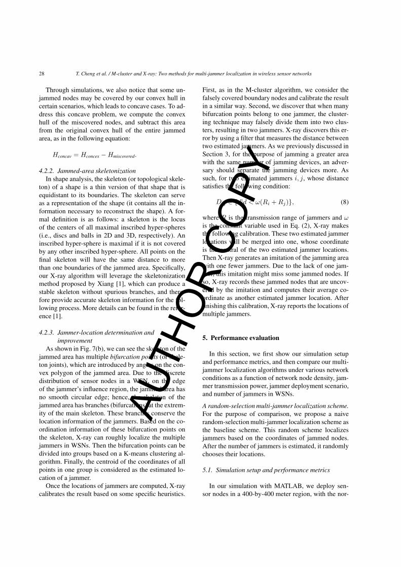
Impact of node density. First, we study the impact ofnode density on the performance of our algorithms. Inthis part, we adjust the total number of nodes by set-ting it to 400, 500 and 600, respectively and calculatethe mean errors for both M-cluster and X-ray. Two sce-narios of simple deployment and mesh deployment areshown in the same figure. From Fig. 9(a), we observethat X-ray has consistently better performance than M-cluster in all node density and node deployment se-tups. In the mesh deployment scenario, X-ray’s meanerrors fall between 6 to 9 meters, while M-cluster’smean errors fall between 8 to 11 meters. M-clusterhas a greater improvement in the localization accuracyas the node deployment model changes from the sim-ple style to the mesh style; in other words, M-clusteris more influenced by the deployment style of sensornodes in WSNs. Meanwhile, both M-cluster and X-rayhave better performance when node density increases.

Fig. 9. Impacts of different conditions on X-ray and M-cluster inmulti-jammer localization: (a) Node density, (b) Jammer transmis-sion range, (c) Jammer number.

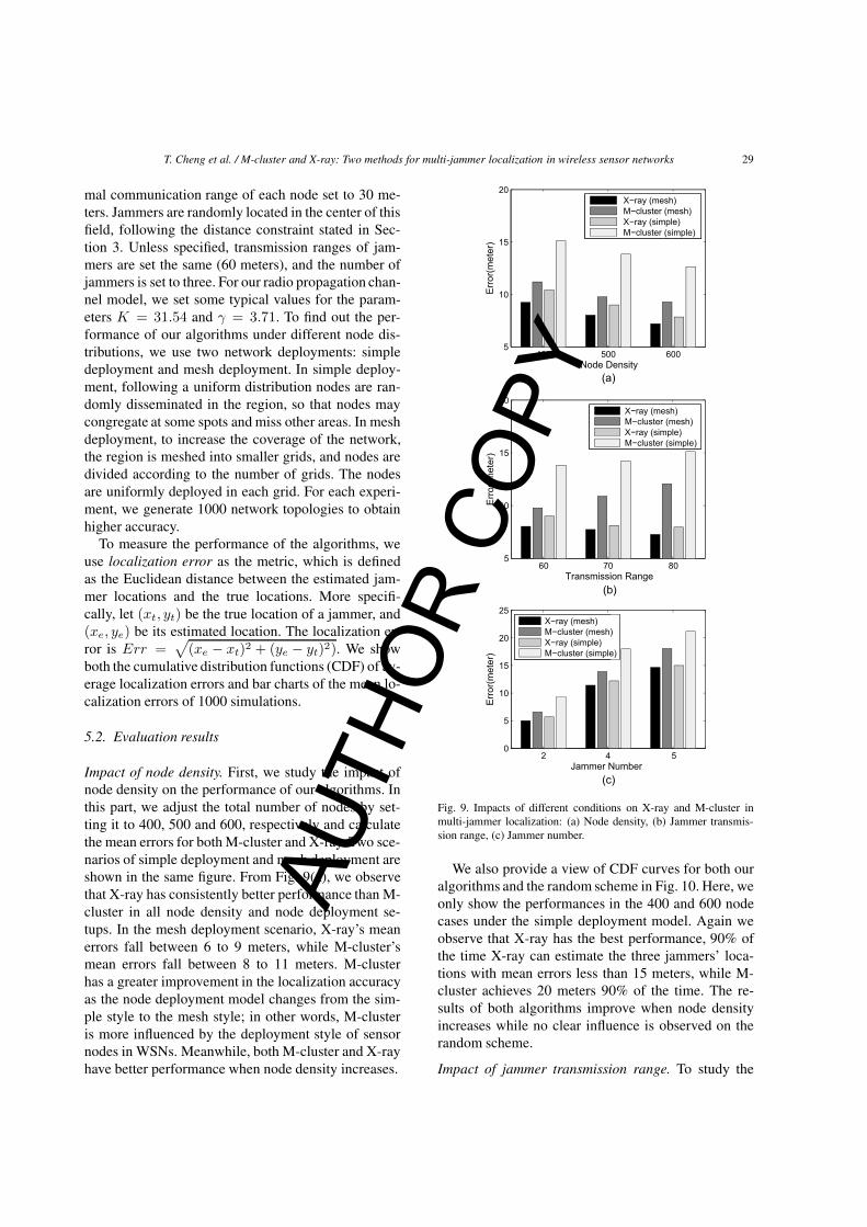
We also provide a view of CDF curves for both ouralgorithms and the random scheme in Fig. 10. Here, weonly show the performances in the 400 and 600 nodecases under the simple deployment model. Again weobserve that X-ray has the best performance, 90% ofthe time X-ray can estimate the three jammers’ loca-tions with mean errors less than 15 meters, while M-cluster achieves 20 meters 90% of the time. The re-sults of both algorithms improve when node densityincreases while no clear influence is observed on therandom scheme.

Impact of jammer transmission range. To study the

AUTH

OR

COPY


Fig. 10. Impact of different node density with the transmission rangeset to 60 meter: (a) N = 400, (b) N = 600.

impact of jammer transmission range on the perfor-mance of our algorithms, we evaluate these algorithmsin two settings: same fixed transmission ranges andrandom transmission ranges. In the fixed transmis-sion range scenario, we fix the jammer’s transmissionranges at 60, 70 and 80 meters, respectively. In therandom transmission range scenario, the jammer trans-mission ranges are randomly chosen from a certainrange in [60, 80], respectively. (Once the transmissionrange is chosen, it would not change in that simula-tion). As a result, each jammer has a different transmis-sion range. From Fig. 9(b), the mean-error figure, weobserve that, with the increase of jammer transmissionrange, X-ray has reduced localization errors, while theerror of M-cluster increases. This is an interesting ob-servation, and it can be explained as follows. As thejammer transmission range increases, the jammed areabecomes bigger; as a result, more sensor nodes are cov-ered in the jammed region. For X-ray, a bigger jammedarea will lead to a larger boundary consisting of morejammed nodes, so more branches on the skeleton ofthe jammed area will be created and X-ray can thenobtain more information about the jammers, improv-ing the final estimation accuracy. For M-cluster, a big-ger jammed area covers more space and nodes. It is

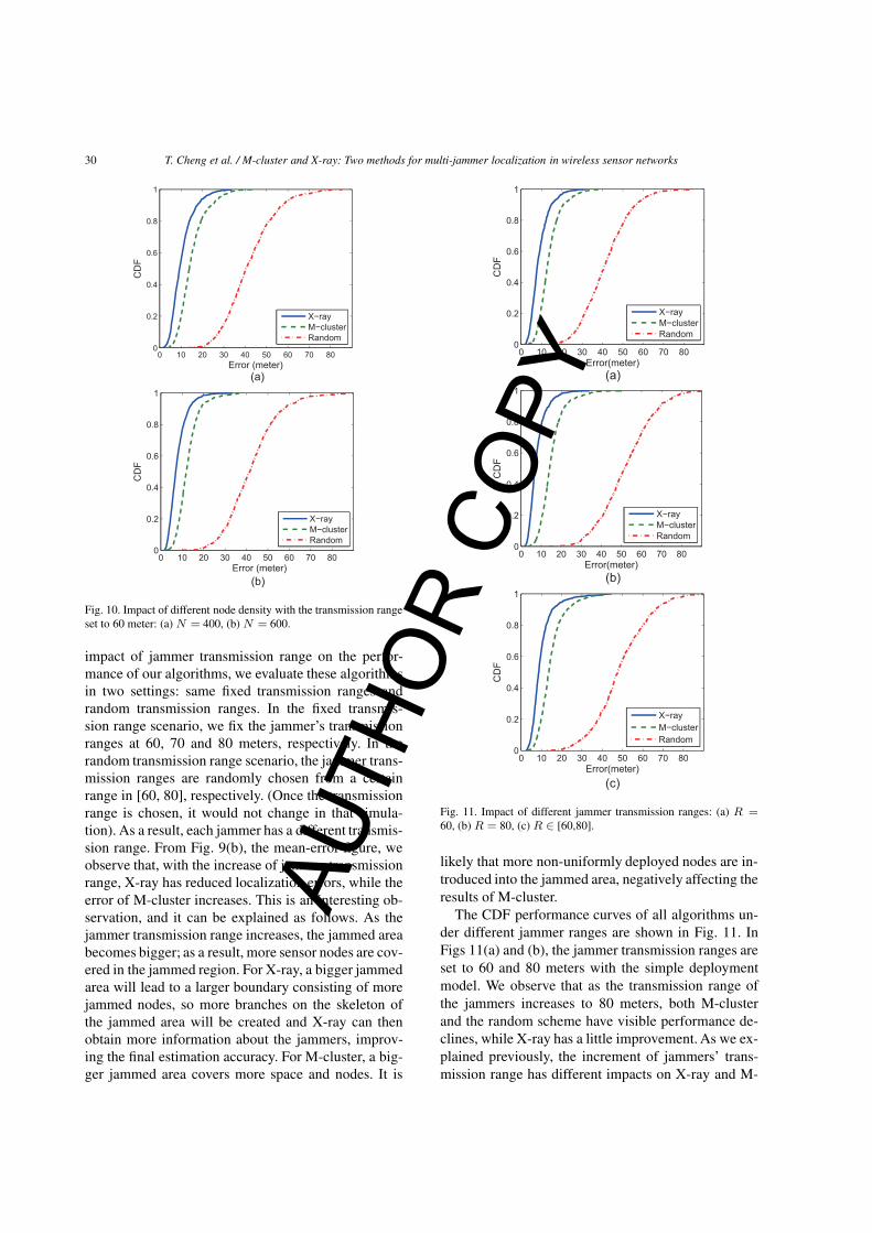
Fig. 11. Impact of different jammer transmission ranges: (a) R =60, (b) R = 80, (c) R ∈ [60,80].

likely that more non-uniformly deployed nodes are in-troduced into the jammed area, negatively affecting theresults of M-cluster.

The CDF performance curves of all algorithms un-der different jammer ranges are shown in Fig. 11. InFigs 11(a) and (b), the jammer transmission ranges areset to 60 and 80 meters with the simple deploymentmodel. We observe that as the transmission range ofthe jammers increases to 80 meters, both M-clusterand the random scheme have visible performance de-clines, while X-ray has a little improvement. As we ex-plained previously, the increment of jammers’ trans-mission range has different impacts on X-ray and M-

AUTH

OR

COPY


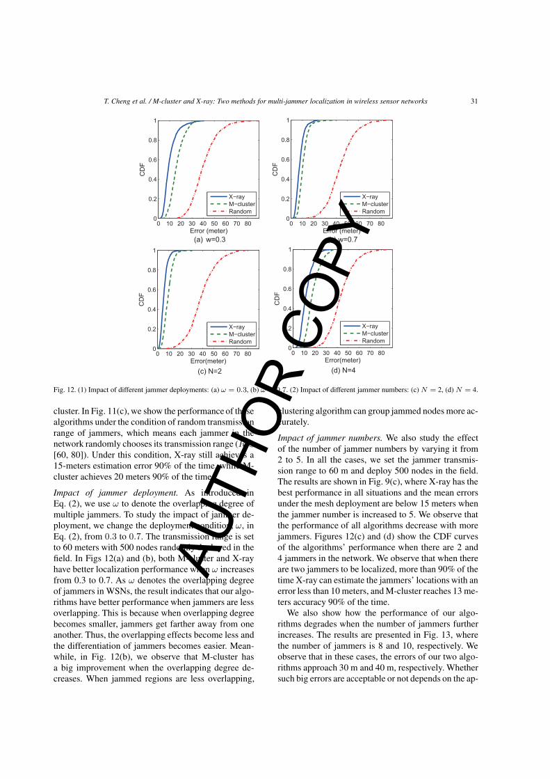
Fig. 12. (1) Impact of different jammer deployments: (a) ω = 0.3, (b) ω = 0.7. (2) Impact of different jammer numbers: (c) N = 2, (d) N = 4.

cluster. In Fig. 11(c), we show the performance of thesealgorithms under the condition of random transmissionrange of jammers, which means each jammer in thenetwork randomly chooses its transmission range (R ∈[60, 80]). Under this condition, X-ray still achieves a15-meters estimation error 90% of the time, while M-cluster achieves 20 meters 90% of the time.

Impact of jammer deployment. As introduced inEq. (2), we use ω to denote the overlapping degree ofmultiple jammers. To study the impact of jammer de-ployment, we change the deployment condition, ω, inEq. (2), from 0.3 to 0.7. The transmission range is setto 60 meters with 500 nodes randomly deployed in thefield. In Figs 12(a) and (b), both M-cluster and X-rayhave better localization performance when ω increasesfrom 0.3 to 0.7. As ω denotes the overlapping degreeof jammers in WSNs, the result indicates that our algo-rithms have better performance when jammers are lessoverlapping. This is because when overlapping degreebecomes smaller, jammers get farther away from oneanother. Thus, the overlapping effects become less andthe differentiation of jammers becomes easier. Mean-while, in Fig. 12(b), we observe that M-cluster hasa big improvement when the overlapping degree de-creases. When jammed regions are less overlapping,

clustering algorithm can group jammed nodes more ac-curately.

Impact of jammer numbers. We also study the effectof the number of jammer numbers by varying it from2 to 5. In all the cases, we set the jammer transmis-sion range to 60 m and deploy 500 nodes in the field.The results are shown in Fig. 9(c), where X-ray has thebest performance in all situations and the mean errorsunder the mesh deployment are below 15 meters whenthe jammer number is increased to 5. We observe thatthe performance of all algorithms decrease with morejammers. Figures 12(c) and (d) show the CDF curvesof the algorithms’ performance when there are 2 and4 jammers in the network. We observe that when thereare two jammers to be localized, more than 90% of thetime X-ray can estimate the jammers’ locations with anerror less than 10 meters, and M-cluster reaches 13 me-ters accuracy 90% of the time.

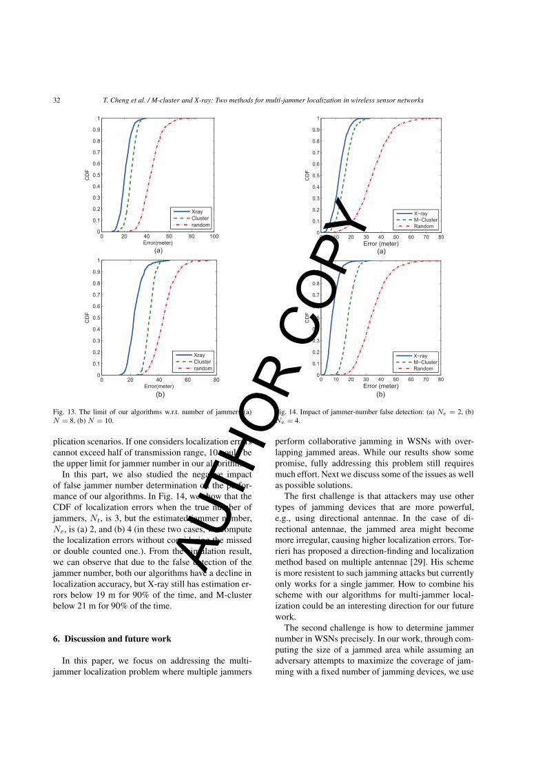
We also show how the performance of our algo-rithms degrades when the number of jammers furtherincreases. The results are presented in Fig. 13, wherethe number of jammers is 8 and 10, respectively. Weobserve that in these cases, the errors of our two algo-rithms approach 30 m and 40 m, respectively. Whethersuch big errors are acceptable or not depends on the ap-

AUTH

OR

COPY


Fig. 13. The limit of our algorithms w.r.t. number of jammers (a)N = 8, (b) N = 10.

plication scenarios. If one considers localization errorscannot exceed half of transmission range, 10 could bethe upper limit for jammer number in our algorithms.

In this part, we also studied the negative impactof false jammer number determination on the perfor-mance of our algorithms. In Fig. 14, we show that theCDF of localization errors when the true number ofjammers, Nt, is 3, but the estimated jammer number,Ne, is (a) 2, and (b) 4 (in these two cases, we computethe localization errors without considering the missedor double counted one.). From the simulation result,we can observe that due to the false detection of thejammer number, both our algorithms have a decline inlocalization accuracy, but X-ray still has estimation er-rors below 19 m for 90% of the time, and M-clusterbelow 21 m for 90% of the time.

6. Discussion and future work

In this paper, we focus on addressing the multi-jammer localization problem where multiple jammers

Fig. 14. Impact of jammer-number false detection: (a) Ne = 2, (b)Ne = 4.

perform collaborative jamming in WSNs with over-lapping jammed areas. While our results show somepromise, fully addressing this problem still requiresmuch effort. Next we discuss some of the issues as wellas possible solutions.

The first challenge is that attackers may use othertypes of jamming devices that are more powerful,e.g., using directional antennae. In the case of di-rectional antennae, the jammed area might becomemore irregular, causing higher localization errors. Tor-rieri has proposed a direction-finding and localizationmethod based on multiple antennae [29]. His schemeis more resistent to such jamming attacks but currentlyonly works for a single jammer. How to combine hisscheme with our algorithms for multi-jammer local-ization could be an interesting direction for our futurework.

The second challenge is how to determine jammernumber in WSNs precisely. In our work, through com-puting the size of a jammed area while assuming anadversary attempts to maximize the coverage of jam-ming with a fixed number of jamming devices, we use

AUTH

OR

COPY


two simple ways to identify the number of jammers.These algorithms are efficient but likely result in in-creased errors as the jammer number goes up. Note thatwhen the jammed areas are disconnected, each individ-ual area can be treated separately with our algorithms.Therefore, the question is how to accurately determinethe number of jammers within one large jammed area.Clearly, if the adversary does not want to maximize hisjamming effect, he may deploy some jamming nodesvery closely (i.e., violating our distance constraint). Asa result, we may not be able to accurately estimate thenumber. Indeed, if the jamming nodes simultaneouslyvary their transmission powers so that they disguisetheir number or if an unjammed area is totally sur-rounded by jammed areas (hence no information aboutthe unjammed nodes can be obtained), jammer-numberidentification could become an undecidable problem.

Fortunately, our ultimate goal is to localize the jam-mers, not to estimate their numbers. As such, we canhave some additional mechanisms to improve the ac-curacy. First, we may overcome the limitation by scan-ning the results of the possible jammer numbers (con-sidering not only the calculated jammer number n, butalso the numbers n − 1 and n + 1), and choose thebest matched estimation result. Second, the defenderis not limited to a single round of localization. It caniteratively localize the jammers in a jammed area un-til no jammer remains. That is, after each round of lo-calization, the localized jammers will be removed ordestroyed immediately and the localization algorithmwill be run again when jamming continues. Third, wemay improve the localization accuracy of our algo-rithms. In M-cluster, we only choose the coordinatesof jammed nodes as the clustering features; however,some other information may be used to improve finalpartitions; e.g., RSS of jammed nodes.

In our simulation results, we discover M-clusteris not as good as X-ray under the proposed differ-ent conditions. However, compared with X-ray, M-cluster has some considerable advantages on compu-tational complexity (much less computation than X-ray) and practical flexibility (no reliance on the avail-ability of a jammed-area mapping service [31] that isitself very complex). In our M-cluster algorithm, wechoose node coordinates as the feature used in clus-tering algorithms, while other characteristics might beextracted to improve the grouping results. This is ourfuture direction to improve the M-cluster algorithm. Inthe X-ray algorithm, we choose the convex envelope tocompute the jammed area, as it is efficient and suitableto derive a unique simple skeleton by the skeletoniza-

tion technique. However, some information may be un-available due to the requirement of convexity. A futureimprovement of X-ray would be to generate a more ac-curate jammed area that can preserve the most infor-mation of jammers. In conclusion, choosing M-clusteror X-ray is primarily a trade-off between localizationaccuracy and computational requirements.

7. Conclusion

This paper studied a multi-jammer localization prob-lem in wireless sensor networks and proposed twomulti-jammer localization algorithms: M-cluster andX-ray. The algorithms attempt to determine the loca-tions of multiple jammers in WSNs in one run. Wemade our comprehensive simulation and comparison,and applied our algorithms under variable conditionsincluding different node densities, transmission ranges,overlapping degrees, and jammer numbers. The sim-ulation results show that our algorithms achieve goodperformance in localizing the jammers under the di-verse situations. Future directions include an improvedjamming propagation model with shadowing and fad-ing, more accurate determination of jammer number,and further improvement of both X-ray and M-cluster.

Acknowledgments

We thank the reviewers for their valuable feedbackwhich greatly helped improve the work. The workof Sencun Zhu was supported in part by the grantW911NF-11-2-0086 from the Army Research Labo-ratory (ARL) and the U.S. NSF CAREER 0643906.The views and conclusions contained here are those ofthe authors and should not be interpreted as necessar-ily representing the official policies or endorsements,either express or implied, of ARL or NSF.

References

[1] X. Bai, L.J. Latecki and W.-Y. Liu, Skeleton pruning by con-tour partitioning with discrete curve evolution, in: IEEE TransPattern Anal Mach Intell (2007), 449–462.

[2] Z. Bankovic, J.M. Moya, A. Araujo, D. Fraga, J.C. Vallejoand J.-M. de Goyeneche, Distributed intrusion detection sys-tem for wireless sensor networks based on a reputation systemcoupled with kernel self-organizing maps, Integr Comput-Aided Eng 17(2) (April 2010), 87–102.

[3] M. Çakiroglu and A.T. Özcerit, Jamming detection mecha-nisms for wireless sensor networks, in: InfoScale ’08: Pro-ceedings of the 3rd International Conference on Scalable In-formation Systems (2008), 4:1–4:8.

AUTH

OR

COPY


[4] F. Chang, C.-J. Chen and C.-J. Lu, A linear-time component-labeling algorithm using contour tracing technique, in: Com-puter Vision and Image Understanding (2004), 206–220.

[5] T. Cheng, P. Li and S. Zhu, Multi-jammer localization inwireless sensor networks, in: Proceedings of InternationalConference on Computational Intelligence and Security (CIS)(2011).

[6] T. Cheng, P. Li and S. Zhu, An algorithm for jammer local-ization in wireless sensor networks, in: Proceedings of The26th IEEE International Conference on Advanced Informa-tion Networking and Applications (AINA) (2012).

[7] J.T. Chiang and Y.-C. Hu, Dynamic jamming mitigation forwireless broadcast networks, in: IEEE Infocom, (2008).

[8] T.H. Cormen, C. Stein, R.L. Rivest and C.E. Leiserson, Intro-duction to algorithms, McGraw-Hill Higher Education, 2ndedition, 2001.

[9] Q. Dong and D. Liu, Adaptive jamming-resistant broadcastsystems with partial channel sharing, in: Proceedings of theInternational Conference on Distributed Computing Systems(ICDCS), 2010.

[10] A. Goldsmith, Wireless commulications, Cambridge Univer-sity Press, 2005.

[11] A. Habib and M. Rupp, Antenna selection in polarized multi-ple input multiple output transmissions with mutual coupling,Integrated Computer-Aided Engineering (2012), 299–312.

[12] X. Jiang, W. Hu, S. Zhu and G. Cao, Compromise-resilientanti-jamming for wireless sensor networks. In Wirel CommunMob Comput Wireless Networks, 17 (2011).

[13] J. Kim, H. Jeon and J. Lee, Network management frameworkand lifetime evaluation method for wireless sensor networks,Integrated Computer-Aided Engineering (2012), 165–178.

[14] M. Li, I. Koutsopoulos and R. Poovendran, Optimal jam-ming attacks and network defense policies in wireless sen-sor networks, in: INFOCOM’07: Proceedings of the 26thIEEE International Conference on Computer Communica-tions. (2007), 1307–1315.

[15] H. Liu, Z. Liu, Y. Chen and W. Xu, Localizing multiple jam-ming attackers in wireless networks, in: ICDCS’11: Proceed-ings of Int’l Conference on Distributed Computing Systems(2011), 517–528.

[16] H. Liu, W. Xu, Y. Chen and Z. Liu, Localizing jammers inwireless networks, in: PERCOM’09: Proceedings of the 2009IEEE International Conference on Pervasive Computing andCommunications (2009), 1–6.

[17] Y. Liu and P. Ning, Bittrickle: Defending against broadbandand high-power reactive jamming attacks, in: Proceedingsof IEEE International Conference on Computer Communica-tions (Infocom) (2012).

[18] Z. Liu, H. Liu, W. Xu and Y. Chen, Wireless jamming local-ization by exploiting nodes’ hearing ranges, in: DCOSS’10:Proceedings of the International Conference on DistributedComputing in Sensor System (2010), 348–361.

[19] G. Mao, B. Fidan and B.D.O. Anderson, Wireless sensor net-

work localization techniques, in: Comput Netw 51 (2007),2529–2553.

[20] S. Misra, R. Singh and S.V.R. Mohan, Information warfare-worthy jamming attack detection mechanism for wireless sen-sor networks using a fuzzy inference system, in: Sensors 10(2010), 3444–3479.

[21] A. Mpitziopoulos and D. Gavalas, An effective defensivenode against jamming attacks in sensor networks, in: Securityand Communication Networks 2 (2009), 145–163.

[22] K. Pelechrinis, M. Iliofotou and S.V. Krishnamurthy, Attacksin wireless networks: The case of jammers, in: IEEE CommunSurveys Tuts 13 (2011).

[23] F.P. Preparata and S.J. Hong, Convex hulls of finite sets ofpoints in two and three dimensions, in: Commun ACM (1977).

[24] S. Roger, C. Ramiro, A. Gonzalez, V. Almenar and A. Vidal,An efficient gpu implementation of fixed-complexity spheredecoders for mimo wireless systems, Integrated Computer-Aided Engineering (2012), 341–350.

[25] M. Strasser, B. Danev and S. Capkun, Detection of reac-tive jamming in sensor networks, in: ACM Trans Sen Netw 7(2010), 16:1–16:29.

[26] M. Strasser, C. Pöpper and S. Capkun, Efficient uncoordinatedfhss anti-jamming communication, in: MobiHoc’09: Proceed-ings of the Tenth ACM International Symposium on Mobile adHoc Networking and Computing (2009), 207–218.

[27] P. Tague, M. Li and R. Poovendran, Mitigation of controlchannel jamming under node capture attacks, in: IEEE Trans-actions on Mobile Computing 8 (2009).

[28] D. Torrieri, Principles of spread-spectrum communicationsystems, 2nd ed., Springer, 2011.

[29] D. Torrieri, Direction finding of a compromised node in aspread-spectrum network, in: MILCOM: Proceedings of theIEEE Military Communications Conference (2012).

[30] Q. Wang, P. Xu, K. Ren and X.-Y. Li, Delay-bounded adaptiveufh-based anti-jamming wireless communication, in: INFO-COM’11: Proceedings of the IEEE International Conferenceon Computer Communications (2011).

[31] A.D. Wood, J.A. Stankovic and S.H. Son, Jam: A jammed-area mapping service for sensor networks, in: RTSS’03: Pro-ceedings of the 24th IEEE International Real-Time SystemsSymposium (2003), 286–297.

[32] A.D. Wood, J.A. Stankovic and G. Zhou, Deejam: Defeatingenergy-efficient jamming in ieee 802.15.4-based wireless net-works, in: Proceedings of IEEE SECON’07 (2007).

[33] R. Xu and D. Wunsch, Clustering, Wiley-IEEE Press, 2008.[34] W. Xu, K. Ma, W. Trappe and Y. Zhang, Jamming sensor

networks: Attacks and defense strategies, in: IEEE Network,(2006).

[35] W. Xu, W. Trappe and Y. Zhang, Channel surfing: defend-ing wireless sensor networks from interference, in: IPSN ’07:Proceedings of the 6th International Conference on Informa-tion Processing in Sensor Networks (2007), 499–508.AU

THO

R CO

PY

ios press m-cluster and x-ray: two methods for multi ...sxz16/papers/ica00445.pdf · multi-jammer...

Documents