ionization and transport - cern

Ionization and Transport

21st FLUKA Beginners’ CourseALBA Synchrotron (Spain)

April 8-12, 2019

OverviewWe will briefly discuss the following interaction mechanisms of charged projectiles traversing a material:

- Ionization losses: energy loss in collisions with target electrons.

- Collisions of charged projectiles with (screened) Coulomb potential of nuclei (Multiple) Coulomb scattering.

In addition to giving a glimpse of FLUKA’s approach to these interaction mechanisms (and FLUKA options governing them), we address here the concept of transport thresholds and transport in magnetic fields.

FLUKA Beginners' Course 2

In a “detailed” Monte Carlo simulationMC: simulate ensemble of particle trajectories + statistical analysis of desired observables.

For each type of event: differential cross section (dxs) → energy loss T, deflection angle.

E.g. ionization losses and Coulomb scattering with target atoms

Ideally one would simulate each particle trajectory event by event (detailed simulation): take step, decide interaction type, sample from dxs, update ene/dir… and loop.


…is this feasible in practice?


Estimate number of ionization lossesRough estimate of number of ionization losses to sample per primary: range/IMFP.

For a 1-MeV e-: range/IMFP ~ 10000 events (!) -> Too many to simulate explicitly.

Electrons in Al

IMFP: inelastic mean free path(EMFP: elastic mean free path)


A more practical approachCondensed simulation schemes are a practical necessity to keep CPU time within acceptable bounds.

Main idea in scheme adopted in FLUKA:- Sample ionization losses explicitly only when the effect is large- Account for global effect of small losses in an effective way

(to be briefly discussed here) along each particle step.

In this session: brief overview of FLUKA’s condensed transport scheme for ionization (as well as multiple Coulomb scattering). 6

Ionization energy losses

Energy losses of charged projectiles in collisions with the electrons of the medium


Ionization energy losses in FLUKA

0 Tδ

Energy loss T

2 different treatments: small vs large energy losses.

Tmax


T>Tδ: Discrete losses

Large loss T transferred to a target electron.

Invested in “releasing” and setting in motion this knock-on electron (δ ray).

δ rays are typically energetic and can transport energy away from their point of origin, so it makes sense to sample their production and transport explicitly (discrete losses).

… how is T sampled?

Tδ Tmax0

Energy loss T


T>Tδ: detailed samplingDepending on projectile, discrete energy losses are sampled from:

Specific expressions:• Møller scattering (e-)• Bhabha scattering (e+)• Mott cross section for heavy ions.

T is sampled from these differential cross section according to projectile type.

All moments reproduced: average energy loss, fluctuations, etc

+

+−=

−=

2

20

22

2

2

2

21

22

2

2

2

0

2112

12

McTT

TT

Tcmr

dTd

TT

Tcmr

dTd

e

max

e

e

ee

e

max

e

e

ee

e

ββπσ

ββπσ


δ-ray production threshold

• Probability of explicit δ-ray production depends on Tδ (δ-ray production threshold).

• FLUKA sets default values, can be overridden (rule of thumb below):

Electrons,positrons: EMFCUT card with PROD-CUT sdum; (see note after MCS for WHAT(3)=FUDGEM)

Charged hadrons/muons: set by DELTARAY card:

where:δThresh production threshold, (from materials Mat1 to Mat2)Ntab, Wtab control the accuracy of dp/dx tabulations (advanced user)PRINT if set (not default), dp/dx tabulations are printed on stdout

* ..+....1....+....2....+....3....+....4....+....5....+....6....+....7..DELTARAY δThresh Ntab Wtab Mat1 Mat2 StepPRINT

* ..+....1....+....2....+....3....+....4....+....5....+....6....+....7..EMFCUT ElePosiTh WHAT(2) WHAT(3) Mat1 Mat2 StepPROD-CUT

Tδ Tmax

Energy loss T0

11

Continuous losses (T<Tδ)

Cross sections go like T-2 → Small losses are frequent → (too much CPU effort to sample them individually).

Idea: account for the aggregate effect of these small losses below the production threshold as a continuous energy loss at each particle step.

For a given step, the continuous energy loss can be calculated by determining the mean energy loss below the production threshold according to restricted

stopping powers (next slide) and by applying energy loss fluctuations on top to account for the stochastic nature of energy

loss (next slide+2)

The energy deposition due to the continuous energy loss of charged particles is local(i.e. energy not carried away by secondary particles)

Tδ Tmax0

Energy loss T


Charged particle dE/dx: Bethe-BlochSpin 0 (spin 1/2 is similar):

ne : electron density of target material (~ Z/A); I : target mean excitation energy, material-dependent; Tmax : maximum energy transfer to an electron (from kinematics)

(Bethe formula derived within 1st Born approx: 1st-order perturbation theory and plane waves, assuming v>>ve)

To improve shortcomings, a series of corrections are used:

δ : density correction; C : is the shell correction, important at low energies L1 : Barkas correction (z3). L2 : Bloch (z4) correction. G : Mott corrections.


+−−++−

−

=

G

ZCLzzL

ITcmzcmrn

dxdE eeee δβββ

ββ

βπ 2)(2)(22

)1(2ln2

22

12

22max

22

2

222

0

∼ln β4γ4 relativistic rise

FLUKA’s approach to loss fluctuations• Aggregate energy loss in a step is sum of n individual losses T~dσ/dT, where n~Poisson and dσ/dT

is the distribution of energy losses for each charged projectile.

• Mathematical machinery: sampling aggregate energy loss distribution in a step from the cumulants of dσ/dT (see extra slides):

• Cumulants and all necessary integrals can be calculated analytically and exactly a priori (minimal

CPU time penalty).

• Applicable to any kind of charged particle, taking into account the proper spin dependent cross

section for δ ray production;

• The first 6-moments of the energy loss distribution are reproduced


Energy-dependence in step and material parametersBelow the δ-ray threshold, energy losses are treated as “continuous”, with some specialfeatures:

• Fluctuations of energy loss are simulated with a cumulant-based FLUKA-specificalgorithm.

• The energy dependence of discrete-loss cross sections and dE/dx along the step istaken into account exactly.

• User has control on dE/dx parameters. The latest recommended values of meanexcitation energy (I) and density effect parameters are implemented for each element(Sternheimer, Berger & Seltzer), but can be overridden by the user (e.g. compounds)via the following cards:

* ..+....1....+....2....+....3....+....4....+....5....+....6....+....7..STERNHEI C X0 X1 a m δ0 MAT*MAT-PROP Gasp Rhosc Iion Mat1 Mat2 Step


Energy loss distributions

Experimental 1 and calculated energy loss distributions for 2 GeV/c positrons (left) and protons (right) traversing 100μm of Si [1] J.Bak et al. NPB288, 681 (1987)


Same scheme for all charged projectiles As discussed above, ionization energy loss scheme in FLUKA is set up in such a way that it is

valid for all charged projectiles:

Electrons/positrons Charged hadrons Muons Heavy Ions

All share the same approach!

… but some extra features are needed for Heavy Ions


Heavy ions In addition to “normal” first Born approximation (Bethe-Bloch formula)

Effective charge (up-to-date parameterizations)

Charge exchange effects (dominant at low energies, ad-hoc model developed for FLUKA)

Mott cross section.

Nuclear form factors (of projectile ion!).

Direct e+/e- production.

Ref: Uggerhoj U.I., Matem.-fys. Meddelelser 52 699 (2006)


Heavy ionsDepth-dose distribution of 238U beam in steel (exp data GSI).

Exaggerated/limiting case (wouldn’t be as dramatic for 12C)FLUKA Beginners' Course 19

Bragg peak: 20Ne @ 670 MeV/n

Dose vs depth distribution for 670 MeV/n 20Neions on a water phantom.

Solid line is the FLUKA prediction. The symbolsare exp data from LBL and GSI.

Tail due to fragmentation products (talktomorrow).

Fragmentation products

Exp. Data Jpn.J.Med.Phys. 18, 1,1998


Dose vs depth distribution for 270 and330 MeV/n 12C ions on a water phantom.

The full green and dashed blue lines arethe FLUKA predictions.

The symbols are exp data from GSI.

Exp. Data Jpn.J.Med.Phys. 18, 1,1998

Idem for 12C


Summary We have discussed two separate treatments for ionization energy losses in FLUKA:

discrete vs continuous.

Discrete losses (above delta production threshold) sampled individually.

Continuous losses described effectively along particle step. First 6 moments of energy-loss distribution reproduced thanks to FLUKA’s approach via cumulants of dσ/dT.

Approach is set up in such a way that it works for all charged projectiles considered in FLUKA.

Dedicated effort for ions leads to good agreement with exp.


2/4 - Transport thresholds


Transport thresholdIn a MC simulation particles are not tracked until they “have lost all their kinetic energy”, but until their energy drops to/below a preset transport threshold

EMFCUT card (without SDUM): energy transport threshold for electrons/positrons/gammas can be set REGION BY REGION.

[WHAT(3) not used]

EMFCUT e±Thresh γThresh 0.0 Reg1 Reg2 Step

When a particle’s energy drops below threshold, what happens?

It is deposited on the spot (for electrons) or ranged out (for heavier projectiles).


Transport thresholds (non EM)

PART-THR card: allows to set transport threshold for hadrons, ions, muons and neutrinos globally for the entire geometry setup

Can be individually set for different particle types, or for all particles.

Neutrons are are special -> The neutron threshold (rounded to closest group boundary), recommended to leave at the default value (1 x 10-14

GeV). Careful to reset if you set threshold from-to in a rangecontaining neutron.

Heavy ion transport thresholds are derived from that of a He4 ion, scaling with ratio of atomic weight ion/He4.

* ..+....1....+....2....+....3....+....4....+....5....+....6....+....7..PART-THR Thresh Part1 Part2 Step


How to set threshold values?

The thresholds have default settings, depending on the SDUM selected on the DEFAULTS card (examine manual)

DO NOT RELY on them, choose those which are best suited for your problem (see next slides)

Guidelines to set threshold energies?


Example• Suppose geometry or scoring grid with dimensions h,w ~ 50 microns

• Let 10-MeV electrons impinge from the left.

What are appropriate threshold values?

Naively: track electrons as long as they can travel farther than one bin width.

Basic idea: put transport threshold at energy such that the range is smaller than bin width.


Examine the particle’s rangeE.g. https://physics.nist.gov/PhysRefData/Star/Text/ESTAR.html

28

Range for electrons in waterWater density: 1 g/cm3 → We may directly read range in cm

Transport threshold at 1 MeV? 1-MeV e- Range is O(1 mm) = 1000 umDepositing/killing them on the spot in a ~50 um geometry is asking too much...

Transport threshold at 10 keV? 10-keV e- range is O(10-4) cm = O(1 um) Depositing them on the spot in a ~50 um geometry is fine

If you’re working with coarser geometries or scoring grids, higher thresholds can be OK!

Note doubledecade jumpin the ordinates…

29

How to set threshold values? General guidelines to set threshold energies?

It depends on the “granularity” of the geometry and/or of the scoring mesh. Energy/range tables are very useful.

Consider the interest in a given region. Warning 1: to reproduce correctly electronic equilibrium, neighboring regions should have the

same electron energy (NOT range) threshold. To be kept in mind for sampling calorimeters Warning 2 : Photon thresholds should be lower than electron thresholds (photons travel farther) Warning 3: low thresholds for e-/ e+/ gammas are CPU eaters

Delta-ray production threshold: If production threshold < transport threshold: CPU wasted in producing and dumping

particles on the spot If production threshold > transport threshold: the latter is increased.


Electron/Photon transport thresholds in the .out file

Ecut: electron transport threshold, given as TOTAL ENERGY in MeV

Pcut: photon transport threshold, given in MeV


Other particle transport thresholds

32FLUKA Beginners' Course 32

Electron/Photon production thresholds in the .out file

Ae: delta-ray production threshold, given as TOTAL ENERGY in MeVAp: photon production threshold, given in MeV


3/4: Multiple Coulomb scattering

Description of potential scattering with screened atomic nuclei


The problem• Besides ionization energy losses, charged particles undergo Coulomb

scattering by (screened) atomic nuclei.

• These collisions are also frequent.

• It is often impractical to sample them all individually.

• One needs effective scheme to sample global effect of Coulomb collisions along a step.

• Formally: what is the distribution of angles after a given step length? What does the spatial distribution look like?

• Approach: specify dxs in individual collision and solve transport equation (with reasonable approx.) to obtain distribution of angles after a traveled path length. 35

Single scattering cross section

At the heart of the approach: assume that in a single Coulomb collision the differential cross section is:

i.e., Rutherford differential cross section with screening parameter.

Advantage: can be integrated analytically for any projectile/material.


Multiple scattering distributionAngular distribution after a given step length?

Molière obtained it from transport equation with approximations:

- Small-angle approximation to the single-scattering cross section.- Number of collisions is large enough (above say 10 or 20).- ...which leads to a minimum applicable step length (!!!!)

Advantage: expressions are simple and depend only parametrically on projectile charge and material properties (!).

Just to see what it looks like, distribution of angles after path length t:

Main idea: every time that the projectile takes a step t, we sample the aggregate deflection from FMol.

( ) ( ) ( )

( ) ( )n

n

Mol

uuJuun

f

fB

fB

tF

=

+++=Ω

∫∞

−

4uln

4ed

!1

sin...11e2d2d,

224/u-

0 0

21

221

2

2

χχ

θθχχχπχθ χ


The FLUKA MCS

Care is taken to maintain relationships among various quantities (correlations):scattering angle ↔ longitudinal displacement

longitudinal displacement ↔ lateral displacement Path length correction ↔ lateral deflection

Careful geometry tracking near boundaries.

MCS is able to coexist with transport in magnetic fields


User control of MCS There are situations where MCS based on Molière theory (despite all efforts) is not applicable:

transport in residual gas, interactions in thin geometries like wire scanners or thin slabs, electronspectroscopies at low energies, microdosimetry, etc.

FLUKA allows user to control various MCS parameters, as well as to switch to detailed singlescattering if needed (CPU demanding, but affordable and accurate e.g. at low electron energies, canbe tuned x material!).

Relevant FLUKA card (to be used on a per-material basis):

Details in FLUKA manual, but essentially:− Switch to single scattering mode.− Spin-relativistic corrections and nuclear finite size effects.

* ..+....1....+....2....+....3....+....4....+....5....+....6....+....7..MULSOPT Flag1 Flag2 Flag3 Mat1 Mat2 StepSDUM

39

Combined result of model effort As a result, FLUKA can correctly simulate electron backscattering even at very low energies

and in most cases without switching off the condensed history transport (a real challenge for an algorithm based on Moliere theory!)

The same algorithm is used for charged hadrons and muons (!).

1.75-MeV electrons on 0.364g/cm2 layer of Cu foil

Transmitted (forward) and backscattered (backward) electron angular distributions

Dots: measured Curves: FLUKA


The FUDGEM parameterIn EMFCUT with SDUM=PROD-CUT, WHAT(3) accounts for the fraction of atomic electrons contributing to MCS.

In Rutherford xs: Z2 Z(Z+f) f=WHAT(3)

A value of 10-5 is fine for low delta-ray production thresholds: the contribution of atomic electrons is accounted for via ionization losses. Low means much lower than typical atomic shell binding energies (several 10s of keV).

For higher delta-ray production thresholds, if WHAT(3)<<1, there would be a fraction of atomic electrons not contributing to scattering. WHAT(3) should be set to 1.

A finite value should be entered for WHAT(3), otherwise:*** Atomic electron contribution to MCS for material …. Set to zero.Are you sure?****

* ..+....1....+....2....+....3....+....4....+....5....+....6....+....7..EMFCUT ElePosiTh WHAT(2) WHAT(3) Mat1 Mat2 StepPROD-CUT


3/4: Summary

We have given a general overview of FLUKA’s approach to multiple Coulomb scattering.

Based on the Moliere theory, with additional effort to maintain various correlations and careful treatment near boundaries.

Possibility to switch to single-scattering mode for delicate situations.

Even for demanding situations like electron backscattering the model performs well!


Cheat Sheet

EMFCUT – Set δ-ray production and transport threshold (e-,e+)DELTARAY – Modify δ-ray production parameters (hadrons, muons)PART-THR - Set particle transport threshold (hadrons, muons)

STERNHEI - Ionization potential and density effectMAT-PROP – Material parameter customization

Some of the ionization, transport, and MCS cards:


4/4 – Transport in magnetic fields


Magnetic field tracking in FLUKAFLUKA allows for tracking in arbitrarily complex magnetic fields. Magnetic field tracking is performed by iterations until a given accuracy when crossing a boundary is achieved. Meaningful user input is required when setting up the parameters defining the tracking accuracy.

Furthermore, when tracking in magnetic fields FLUKA accounts for:

The decrease of the particle momentum due to energy losses along a given step and hence the corresponding decrease of its curvature radius. Since FLUKA allows for fairly large (up to 20%) fractional energy losses per step, this correction is important in order to prevent excessive tracking inaccuracies to build up, or force to use very small steps

The precession of the MCS final direction around the particle direction: this is critical in order to preserve the various correlations embedded in the FLUKA advanced MCS algorithm

The precession of a (possible) particle polarization around its direction of motion: this matters only when polarization of charged particles is a issue (mostly for muons in Fluka)


How to define a magnetic field Declare the regions with field in the ASSIGNMAT card (what(5))

Set field/precision with the card MGNFIELD:

Ifthe field is UNIFORM set its components (in Tesla) in Bx, By, Bz

If not, leave Bx=By= Bz=0 and provide a magnetic field pointwise through the user routine MAGFLD (see later)

α, ε, Smin control the precision of the tracking, (see next slides). They can be overridden/complemented by the STEPSIZE card

* ..+....1....+....2....+....3....+....4....+....5....+....6....+....7..MGNFIELD α ε Smin Bx By Bz


Magnetic field tracking in FLUKA

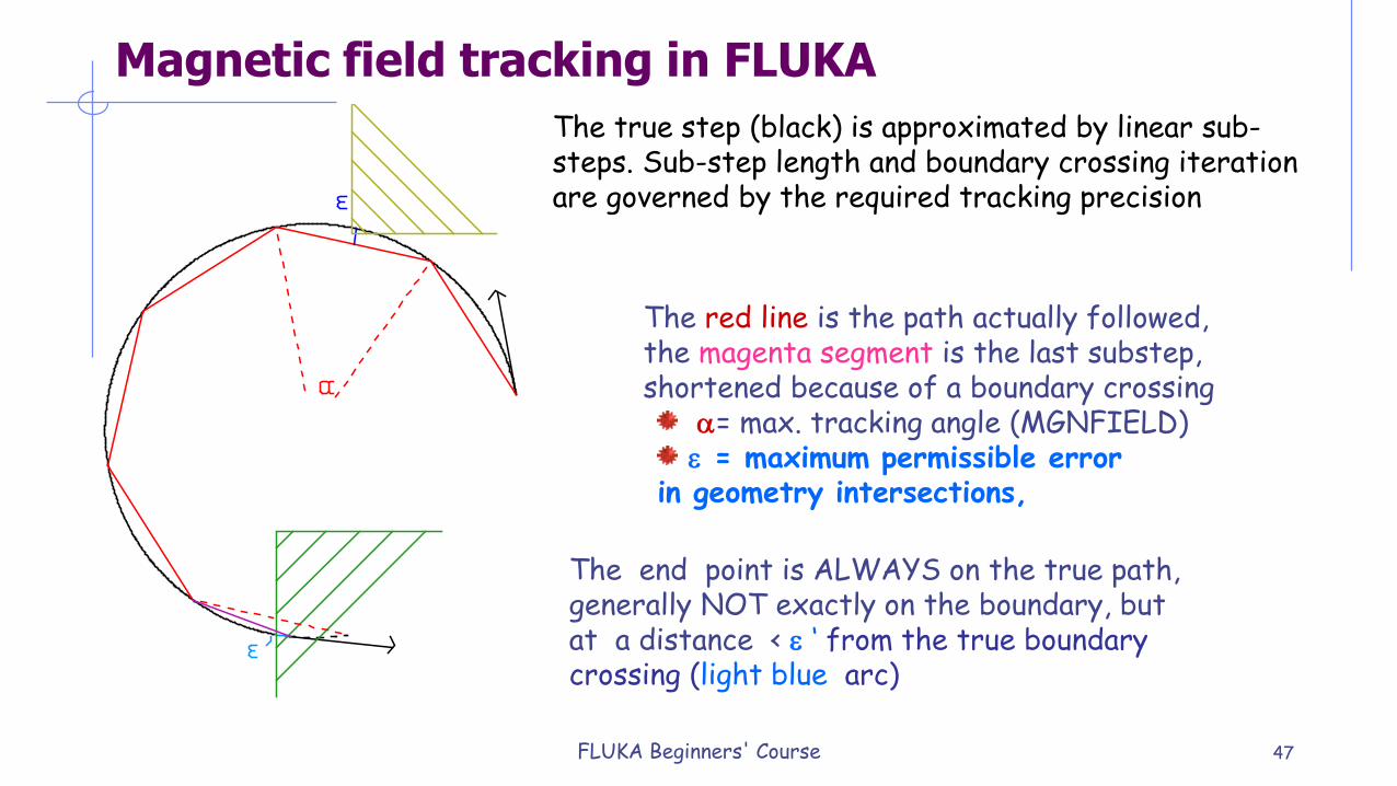
The red line is the path actually followed, the magenta segment is the last substep, shortened because of a boundary crossing

α= max. tracking angle (MGNFIELD)ε = maximum permissible error

in geometry intersections,

The true step (black) is approximated by linear sub-steps. Sub-step length and boundary crossing iterationare governed by the required tracking precision

The end point is ALWAYS on the true path,generally NOT exactly on the boundary, but at a distance < ε ‘ from the true boundary crossing (light blue arc)


Setting the tracking precision I

α largest angle in degrees that a charged particle is allowed to travel in a single sub-step. Default = 57.0 (but a maximum of 30.0 is recommended!)

ε upper limit to error of the boundary iteration in cm (ε’ in fig.). It also sets the tracking error ε. Default = 0.05 cm IF α and/or ε are too large, boundaries may be missed

(as in the plot);

IF they are too small, CPU time explodes....Both α and ε conditions are fulfilled during tracking. Set them according to your problem Tune ε by region with the STEPSIZE card Be careful when very small regions exists in your setting : ε must be smaller than the region dimensions!



Example: Gas Bremsstrahlung


Gas BremsstrahlungIn spite of the high or ultra-high vacuum in storage rings, residual gas molecules lead to an observable effect:

• Electrons impinging on them may lead to the emission of Bremsstrahlung photons.

• E.g. for GeV electrons Bremsstrahlung photons up to ~GeV.

• Photons at these energies are much more penetrating than synchrotron light, which typically does not exceed O(100 keV).

• Thus, there is a radiation hazard.

• It is therefore important to make preliminary studies assessing the dose due to residual-gas Bremsstrahlung.

50

Gas Bremsstrahlung in FLUKA• We cannot do a simulation at the actual density corresponding to 10-9 mbar.

• Main idea: we do a simulation at an artificially higher density, and linearly scale down the results a posteriori to the actual gas density.

• At high densities, however, there are effects leading to the angular broadening of the electron beam which are not present at low densities (i.e. do not scale with density) and should be effectively switched off:

51

…

ExampleADONE e+e- storage ring (INFN-Frascati, 1980s-1990s):

Relevant machine section for this example:• 613.5 cm long straight section (residual gas at 10-9-10-10 Torr)• …followed by a 190.7 cm long vacuum guide • …topped by a 1.87 cm thick stainless steel flange• …surrounded by air (atmospheric pressure).

The detector:• Thermoluminiscent LiF dosimeter (TLD), 3.175x3.175x0.889 mm3

• Arranged in 9x9 matrix: 28.57x27.57 mm2

• Various TLD matrices at various distances after straight section.

TLD matricesFlangeVacuum guide(end of)Straight section

FLUKA Beginners' Course52

Example and references

Relevant references with many more details:Ferrari A. et al., Nucl Instrum Meth B 83 518-524 (1993)Esposito A. et al., Nucl Instrum Meth B 88 345-349 (1994)

Dose (measured vs FLUKA) at the TLD matrix 541.7 cm away from end of straight section:

Open circles: central row… then pairwise away from central row

Exp issues: inhomogeneous pressure


End


Additional material


Topics General settings Interactions of leptons/photons

Photon interactions Photoelectric Compton Rayleigh Pair production Photonuclear Photomuon production

Electron/positron interactions Bremsstrahlung Scattering on electrons

Muon interactions Bremsstrahlung Pair production Nuclear interactions

Ionization energy losses Continuous Delta-ray production

Transport Multiple scattering Single scatteringThese are common to all charged particles, although traditionally associated with EM Transport in Magnetic field


Ionization energy losses in FLUKA

0 Tδ

Energy loss T

T>Tδ: sampled explicitly from corresponding dxs, knock-on electron (δ ray) added to stack of particles to simulate.

T<Tδ : no explicit energy loss sampling / secondary electron tracking.Aggregate effect of many small losses described continuously during particle step.

Tδ : threshold above which it is meaningful to do detailed samplingof knock-on electrons. δ-ray production threshold. User tunable (!)

2 different treatments: small vs large energy losses.

Tmax


Nuclear stopping power Besides collisions with target electrons, charged projectiles undergo

Coulomb scattering with atomic nuclei

The resulting energy losses, called nuclear stopping power, are smaller than the atomic ones, but are important for

Heavy particles (i.e. ions)

Damage to materials:Non-Ionizing Energy Loss (NIEL)Displacements per Atom (DPA)

Scoring built-in.


dpa: Displacements Per Atom FLUKA generalized particle name: DPA-SCO Is a measure of the amount of radiation damage in irradiated

materialsFor example, 3 dpa means each atom in the material has been displaced from its site within the structural lattice of the material an average of 3 times

Displacement damage can be induced by all particles produced in the hadronic cascade, including high energy photons.The latter, however, have to initiate a reaction producing charged particles, neutrons or ions.

The dpa quantity is directly related with the total number of defects (or Frenkel pairs):

ρ atoms/cm3

Ni particles per interaction channel iNf

i Frenkel pairs per channel

∑i

iFi NN

ρ=dpa 1


Control of step size IIStep sizes are optimized by the DEFAULT settings. If the user REALLY needs to change them with:

DEstep should always be below 30% • In most routine problems, a 20% fraction energy loss gives satisfactory results. For

dosimetry, 5-10% should be preferred.WARNING : if a magnetic field is present, it is important to set also a maximum

absolute step length and possibly a precision goal for boundary crossing by means of command STEPSIZE (see later)

For EM

For Had/μ

* ..+....1....+....2....+....3....+....4....+....5....+....6....+....7..EMFFIX Mat1 DEstep1 Mat2 DEstep2 Mat3 DEstep3

* ..+....1....+....2....+....3....+....4....+....5....+....6....+....7..FLUKAFIX DEstep Mat1 Mat2 Step

60

Some warnings about scoring: Every charged particle step Δx has its length constrained by:

Maximum fractional energy loss (see FLUKAFIX) Maximum step size for that region (see STEPSIZE) MCS (or other) physical constraints Distance to next interaction (nuclear, δ ray etc)

The average energy loss is computed as a careful integrationover the dE/dx vs energy curve and then it is fluctuated → a final ΔE is computed and used for scoring → resulting in a scored average effective ΔE/ Δx uniform along that step

The particle energy used for track-length estimators is the average one along the step (E0-ΔE/2)


USRBIN track apportioning scoring

The energy deposition will be Δl/Δx ΔE

Δl

Δx, ΔE


USRBIN track apportioning scoring


USRTRACK scoring: 200 MeV p on C

Default settings, ≈ 20% energy loss per stepFLUKA Beginners' Course 64

Ionization Transport Cheat SheetDELTARAY – Modify δ-ray effect parameters

(for charged hadrons, muons)EMFCUT – Set δ-ray production and transport threshold

(for electrons/positrons)PART-THR - Set particle transport threshold

(for hadron, muons)

STERNHEI - Ionization potential and density effectMAT-PROP parameters customization

IONFLUCT – Set ionization fluctuation options

EMFFIX - Set step size control for electrons/positronsFLUKAFIX – Set step size control for hadrons/muons

MGNFIELD - Set magnetic field precisionSTEPSIZE - Set stepsize in magnetic field


High energies: δ is the so called density correction, extensively discussed inthe literature and connected with medium polarization

Low energies: C is the shell correction, which takes into account the effect ofatomic bounds when the projectile velocity is no longer much larger than thatof atomic electrons and hence the approximations under which the Bethe-Blochformula has been derived break down. This correction becomes important atlow energies.

Higher order: L1 is the Barkas (z3) correction responsible for the differencestopping power for particles-antiparticles, L2 is the Bloch (z4) correction (bothno longer discussed in the following)

Low energies: effective charge. Partial neutralization of projectile charge dueto electron capture, particularly effective at low energies.

Corrections to dE/dx:

66

Landau distribution Lev Landau (1944), assuming: No Bremsstrahlung, only ionization events. Short path lengths ↔ Δ << E, where Δ = total energy loss. Hard events via Thomson cross section:

Distant collisions (small losses): Bethe stopping formula, no fluctuations. Tδ → infinity (Laplace transform involved) With all these approximations, he derived the distribution of energy losses after the

projectile has traveled path length s


FLUKA’s approach to loss fluctuations

- Differences among projectiles are not resolved (Thomson W-2 for all projectiles)

- For distant collisions, no fluctuations.

- Delta-ray cutoff at infinity: cannot be used for too long steps or too low ene!

Landau distribution is somewhat impractical for FLUKA purposes:


Preliminaries: cumulantsProbability density function: f(x)

Characteristic function:

Cumulant generating function:

Cumulants:


Advantages of FLUKA’s approach

• As opposed to Landau distribution (see additional slides), it does

not rely on a particular dσ/dT for ionization!

• Based on general statistical properties of the cumulants of a

distribution (dσ/dT).

• Cumulants and all necessary integrals can be calculated analytically

and exactly a priori (minimal CPU time penalty).

• Applicable to any kind of charged particle, taking into account the

proper spin dependent cross section for δ ray production;

• The first 6-moments of the energy loss distribution are

reproduced.


Ionization fluctuation optionsIonization fluctuations are simulated or not depending on the DEFAULTS used. Can be controlled by the IONFLUCT card:

Remember always that δ-ray production iscontrolled independently and cannot be switchedoff for e+/e- (it would be physically meaningless)

* ..+....1....+....2....+....3....+....4....+....5....+....6....+....7..IONFLUCT FlagH FlagEM Accuracy Mat1 Mat2 STEP


T>Tδ: detailed samplingDepending on projectile, discrete energy losses are sampled from:

• Møller scattering (e-)

• Bhabha scattering (e+)

• δ ray production by spin 0 or ½ projectiles (charged hadrons, muons).• Mott cross section for heavy ions.

T is sampled from these differential xs according to projectile type.All moments reproduced: avg energy loss, fluctuations, etc

−

−−

−+

−

+=

e

ee

e

e

e

ee

Moe TTT

TT

TTT

Tcmr

dTd

02

2

0

22

02

2

2

2 12112γγ

γγ

βπσ

−

−−++

+−

+

−+

−−

++−

−

−+

−−=

00

2

2

2

0

2

2

0

2

02

2

0

2

0

2

02

2

2

2

2

2

112

3121

11

112211

121112

TT

TT

TT

TT

TT

TT

TT

TT

Tcmr

dTd

eee

eee

ee

e

ee

Bhe

γγ

γγγγ

γγ

γγ

γγ

γγ

γγ

γγ

βπσ

72

Energy dependent quantities I Most charged particle transport programs sample the

next collision point by evaluating the cross-section atthe beginning of the step, neglecting its energydependence and the particle energy loss;

The cross-section for δ ray production at low energiesis roughly inversely proportional to the particle energy;a typical 20% fractional energy loss per step would correspond toa similar variation in the cross section

Some codes use a rejection technique based on theratio between the cross section values at the two stependpoints, but this approach is valid only formonotonically decreasing cross sections.


Energy dependent quantities IIFLUKA takes in account exactly the continuous energydependence of:

Discrete event cross section Stopping power

Biasing the rejection technique on the ratio between thecross section value at the second endpoint and itsmaximum value between the two endpoint energies.


Heavy ions dE/dx

Comparison of experimental (R.Bimbot, NIMB69 (1992) 1) (red) and FLUKA (blue) stopping powers of Argon and Uranium ions in different materials and at different energies.


Step size settings for special casesFor typical applications the default 20% fractional energy loss is fine.

For special problems (i.e. thin slabs, microdosimetry, etc) 5-10% is preferred. Stability of results wrt step size should be checked.

If really needed, for EM:

For Had/μ

* ..+....1....+....2....+....3....+....4....+....5....+....6....+....7..EMFFIX Mat1 DEstep1 Mat2 DEstep2 Mat3 DEstep3

* ..+....1....+....2....+....3....+....4....+....5....+....6....+....7..FLUKAFIX DEstep Mat1 Mat2 Step


Maximum step size

Comparison of calculated and experimental depth-dose profiles, for 0.5 MeV e- on Al,with three different step sizes. (2%, 8%, 20%)Symbols: experimental data. r0 is the csda range

Step size is fixed by the corresponding percentage energy loss of the particleThanks to FLUKA mcs and boundary treatment, results are stable vs. (reasonable) step size.First step is where step size matters most.

Moliere: assumes constant energyalong the step (!)

One should not abuse of step length.


Electron Backscattering

Energy(keV)

MaterialExperim.(Drescher et al 1970)

FLUKASingle scattering

FLUKAMultiple scattering

CPU time single/mult ratio

9.3Be 0.050 0.044 0.40 2.73Cu 0.313 0.328 0.292 1.12

Au 0.478 0.517 1.00

102.2Cu 0.291 0.307 0.288 3.00Au 0.513 0.502 0.469 1.59

Fraction of normally incident electrons backscattered out of a surface.All statistical errors are less than 1%.


What about the delta-ray production threshold?

EMFCUT e±Thresh γThresh Fudgem Mat1 Mat2 Step PROD-CUT

Fudgem is related to multiple scattering. = 0 below ≈ 10 keV , = 1 aboveMUST be set, if the field is empty 0

Warning 1: if prod-cut < transport cut, CPU is wasted in producing/dumping particles on spot. Sometimes it could be convenient to define several “equal” materials with different production thresholds (and different names)

Warning 2: if prod-cut > transport cut , the program automatically increases the transport threshold , because it cannot transport a particle that it is not supposed to handle.

EMFCUT with SDUM=PROD-CUT allows to control the threshold for secondary production in any e-/e+/γ interactions

Bremsstrahlung and pair production by muons and charged hadrons (1/2)

PAIRBREM Flag e±Thresh γThresh Mat1 Mat2 Step

PAIRBREM card allows to control the production threshold for bremsstrahlung and pair production by muons, light ions (up to alphas) and charged hadrons

Depending on the DEFAULTS, the processes might be active without explicit production of secondaries (only continuous energy loss treated – see manual)


Bremsstrahlung and pair production by muons and charged hadrons (2/2)

Evidently, the photon transport threshold requested by the EMF-CUTcard should be lower than the Bremsstrahlung production threshold set via PAIRBREM

On the other hand, it is generally recommended to set the e-/e+ pair production threshold to 0 (there is anyway a natural threshold for pair production)

With high thresholds energy loss straggling and energy deposition is not correctly reproduced (but allows to correctly reproduce the average range of muons)


Charged particle transportBesides energy losses, charged particles undergo scattering by atomic nuclei. The Molière multiple scattering (MCS) theory is commonly used to describe the cumulative effect of all scatterings along a charged particle step. However

Final deflection wrt initial direction Lateral displacement during the step Shortening of the straight step with respect to the total trajectory

due to “wiggliness” of the path (often referred to as PLC, path length correction)

Truncation of the step on boundaries Interplay with magnetic field

MUST all be accounted for accurately, to avoid artifacts like unphysical distributions on boundary and step length dependence of the results


The FLUKA MCS Accurate PLC (not the average value but sampled from a

distribution), giving a complete independence from step size Correct lateral displacement even near a boundary Correlations:

PLC ⇔ lateral deflectionlateral displacement ⇔ longitudinal displacement

scattering angle ⇔ longitudinal displacement Variation with energy of the Moliere screening correction Optionally, spin-relativistic corrections (1st or 2nd Born

approximation) and effect of nucleus finite size (form factors) Special geometry tracking near boundaries, with automatic control of

the step size On user request, single scattering automatically replaces multiple

scattering for steps close to a boundary or too short to satisfy Moliere theory. A full Single Scattering option is also available.

Molière theory used strictly within its limits of validity combined effect of MCS and magnetic fields


The FLUKA MCS - II As a result, FLUKA can correctly simulate electron backscattering

even at very low energies and in most cases without switching off the condensed history transport (a real challenge for an algorithm based on Moliere theory!);

The sophisticated treatment of boundaries allows also to deal successfully with gases, very thin regions and interfaces;

The same algorithm is used for charged hadrons and muons.


Single Scattering In very thin layers, wires, or gases, Molière theory does not

apply. In FLUKA, it is possible to replace the standard multiple

scattering algorithm by single scattering in defined materials (option MULSOPT).

Cross section as given by Molière (for consistency) Integrated analytically without approximations Nuclear and spin-relativistic corrections are applied in a

straightforward way by a rejection technique


Magnetic field tracking in FLUKA

The red line is the path actually followed, the magenta segment is the last substep, shortened because of a boundary crossing

α= max. tracking angle (MGNFIELD)ε = max. tracking/missing error

(MGNFIELD or STEPSIZE)ε ‘ = max. bdrx error (MGNFIELD or STEPSIZE)

The true step (black) is approximated by linear sub-steps. Sub-step length and boundary crossing iteration are governed by the required tracking precision

The end point is ALWAYS on the true path,generally NOT exactly on the boundary, but at a distance < ε ‘ from the true boundary crossing (light blue arc) 86

Setting the tracking precision I

α largest angle in degrees that a charged particle is allowed to travel in a single sub-step. Default = 57.0 (but a maximum of 30.0 is recommended!)

ε upper limit to error of the boundary iteration in cm (ε’ in fig.). It also sets the tracking error ε. Default = 0.05 cm

IF α and/or ε are too large, boundaries may be missed ( as in the plot);IF they are too small, CPU time explodes....Both α and ε conditions are fulfilled during tracking. Set them according to your problem Tune ε by region with the STEPSIZE card Be careful when very small regions exists in your setting : ε must be smaller than the region dimensions!


87

Setting precision by region

Smin: (if what(1)>0) minimum step size in cm Overrides MGNFIELD if larger than its setting;

ε (if what(1)<0) : max error on the location of intersection with boundary; The possibility to have different “precision” in different regions allows to

save CPU time. Smax: max step size in cm. Default:100000. cm for a region without

magnetic field, 10 cm with field; Smax can be useful for instance for large vacuum regions with relatively

low magnetic field It should not be used for general step control, use EMFFIX, FLUKAFIX if

needed Settings apply to all charged particles.

* ..+....1....+....2....+....3....+....4....+....5....+....6....+....7..STEPSIZE Smin/ε Smax Reg1 Reg2 Step


Setting the tracking precision II

Smin minimum sub-step length. If the radius of curvature is so small that the maximum sub-step compatible with α is smaller than Smin, then the condition on α is overridden. It avoids endless tracking of spiraling low energy particles. Default = 0.1 cm

Particle 1: the sub-step corresponding to α is > Smin acceptParticle 2: the sub-step corresponding to α is < Smin increase α

Smin can be set by region with the STEPSIZE card



The magfld.f user routineThis routine allows to define arbitrarily complex magnetic fields:SUBROUTINE MAGFLD ( X, Y, Z, BTX, BTY, BTZ, B, NREG, IDISC)

Input variables: x,y,z = current positionnreg = current region

Output variables: btx,bty,btz = cosines of the magn. field vector

B = magnetic field intensity (Tesla) idisc = set to 1 if the particle has to be

discarded

All floating point variables are double precision ones! BTX, BTY, BTZ must be normalized to 1 in double precision


Damage to Electronics

Category Scales with simulated/measured quantity

Single Event effects

(Random in time)

Single Event Upset(SEU) High-energy hadron fluence (>20 MeV)* [cm-2]

Single Event Latchup(SEL) High-energy hadron fluence (>20 MeV)** [cm-2]

Cumulative effects

(Long term)

Total Ionizing Dose(TID) Ionizing Dose [GeV/g]

Displacement damage 1 MeV neutron equivalent [cm-2] NIEL

* Reality is more complicated (e.g.,contribution of thermal neutrons)

** Energy threshold for inducing SEL isoften higher than 20 MeV

DOSE

SI1MEVNE

HADGT20M

Generalized particle


ionization and transport - cern

Documents