investor-owned a mit-ceepr 95-005wp june

System Average Rates of U.S. Investor-OwnedElectric Utilities: A Statistical Benchmark Study

by

Ernst R. Berndt, Roy Epstein, and Michael Doane

MIT-CEEPR 95-005WP June 1995

MASSACHUSETTS INSTITUTE

E•LP 5 1996LURAR!ES

SYSTEM AVERAGE RATES OF U.S. INVESTOR-OWNED ELECTRIC UTILITIES:

A STATISTICAL BENCHMARK STUDY*

by

Ernst R. Berndt, MIT Sloan School of Management

Roy Epstein, Analysis Group, Inc.

Michael Doane, Analysis Group, Inc.

Authors' Addresses:

Ernst R. BerndtMIT Sloan School of

Management50 Memorial Dr., E52-452Cambridge, MA 02142617-253-2665

Roy EpsteinAnalysis Group, Inc.1 Brattle Square,

Fifth FloorCambridge, MA 02138617-349-2179

Michael DoaneAnalysis Group, Inc.100 Bush St., Suite 900San Francisco, CA 94104415-391-6100

*Financial support from San Diego Gas & Electric Company is gratefully

acknowledged, as is the superb research assistance of Laurits R. Christensen

of Analysis Group, Inc. We also acknowledge helpful comments from Robert Dye,

Dr. Larry Schelhorse, and Michael Schneider of San Diego Gas & Electric

Company. The views and opinions expressed in this paper are solely those of

the authors, and do not necessarily reflect positions of San Diego Gas &

Electric Company.

DOCUMENT NAME: ENERGY.JNL DOCUMENT DATE: 8 JUNE 1995

SYSTEM AVERAGE RATES OF U.S. INVESTOR-OWNED ELECTRIC UTILITIES:A STATISTICAL BENCHMARK STUDY

I. INTRODUCTION

Due largely to the fact that they are regulated by public utility

commissions, rates charged by electric utilities are often the focus of

intense public scrutiny. Controversies in rate hearings surrounding

differences in average rates charged residential, commercial and industrial

customers have a long history, but in recent years increasing attention has

focussed on "bottom line" differences across utilities in their overall system

average rates (SARs, revenue per Kwh). Proposals to restructure electric

utilities by, for example, deregulating the generation function and placing

the remaining transmission and distribution functions under some form of

performance-based regulation, or imposing some form of price controls, have

heightened interest in understanding what factors contribute to variations

across utilities in their SARs. State utilities commissions are therefore

examining more closely differences in SARs charged by the various within-state

utilities under their jurisdiction, as well as differences in comparison to

out-of-state utilities.

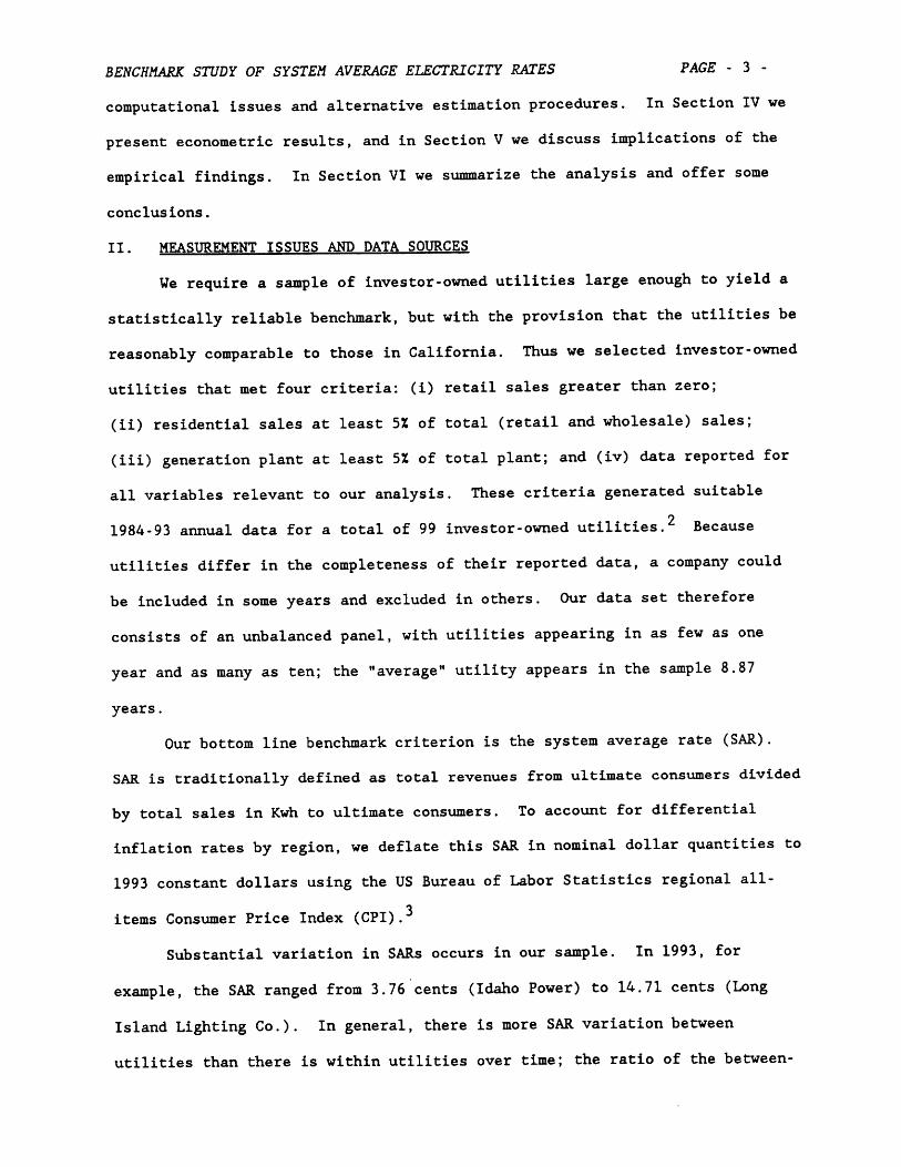
The research reported in this paper emerged from issues brought before

the California Public Utilities Commission (CPUC). California SARs are among

the highest in the US. In 1984, for example, the real (inflation-adjusted)

SAR for San Diego Gas & Electric (SDG&E), Southern California Edison (SCE),

and Pacific Gas and Electric (PG&E) ranked 3, 12 and 24 in comparison with 96

other large investor-owned US electric utilities; a decade later, in 1993, the

respective rankings were 17, 8 and 9. Why are SARs in California so high?

Why are they so much higher than the SARs of, say, Puget Sound Power and

Light, Montana Power Company, Appalachian Power Company, and Idaho Power

Company? Do the high California rates reflect factors largely beyond the

control of utility management, such as the unavailability of low-cost

BENCHMARK STUDY OF SYSTEM AVERAGE ELECTRICITY RATES PAGE - 2 -

generation sources like hydro power and coal; the high local costs of doing

business such as franchise fees, state and local taxes, and state wage rates;

greater regulation-imposed costs such as required conservation and favored

purchasing mandates; or do the high California rates reflect inefficient

management and waste? Understanding why it is that California's SARs are so

high is an essential input in evaluating the likely consequences of

alternative deregulation and price control policy initiatives.

In this paper we report results of a statistical benchmark study

comparing the annual SARs of 99 investor-owned US utilities over the ten-year

time period, 1984-93.1 Our results are based on a statistical model relating

SARs to regional, economic, and regulatory factors largely beyond the control

of utility management, as well as to the effects of management. Following a

tradition originally used in the agricultural economics literature that

focused on estimating production function parameters free of management bias,

we incorporate the effects of management decisions by specifying an error

components model. Using a variety of estimation procedures and data from 99

utilities for up to ten years each, we obtain a surprisingly robust set of

results. Specifically, we find that the SARs of electric utilities are

significantly affected by various regional, economic and regulatory factors.

Controlling for these factors, there is no statistically significant

difference between the SARs charged by the three California utilities and the

national average. Thus, inferences concerning management efficiency made on

the basis of using unadjusted SARs can provide very misleading implications.

The outline of this paper is as follows. In Section II we consider

measurement and data issues. In Section III we develop our econometric model,

and devote particular attention to the error component stochastic

specification. Since our data set consists of an unbalanced panel (not all

utilities have all data available in each of the ten years), we also consider


computational issues and alternative estimation procedures. In Section IV we

present econometric results, and in Section V we discuss implications of the

empirical findings. In Section VI we summarize the analysis and offer some

conclusions.

II. MEASUREMENT ISSUES AND DATA SOURCES

We require a sample of investor-owned utilities large enough to yield a

statistically reliable benchmark, but with the provision that the utilities be

reasonably comparable to those in California. Thus we selected investor-owned

utilities that met four criteria: (i) retail sales greater than zero;

(ii) residential sales at least 5% of total (retail and wholesale) sales;

(iii) generation plant at least 5% of total plant; and (iv) data reported for

all variables relevant to our analysis. These criteria generated suitable

1984-93 annual data for a total of 99 investor-owned utilities.2 Because

utilities differ in the completeness of their reported data, a company could

be included in some years and excluded in others. Our data set therefore

consists of an unbalanced panel, with utilities appearing in as few as one

year and as many as ten; the "average" utility appears in the sample 8.87

years.

Our bottom line benchmark criterion is the system average rate (SAR).

SAR is traditionally defined as total revenues from ultimate consumers divided

by total sales in Kwh to ultimate consumers. To account for differential

inflation rates by region, we deflate this SAR in nominal dollar quantities to

1993 constant dollars using the US Bureau of Labor Statistics regional all-

items Consumer Price Index (CPI).3

Substantial variation in SARs occurs in our sample. In 1993, for

example, the SAR ranged from 3.76 cents (Idaho Power) to 14.71 cents (Long

Island Lighting Co.). In general, there is more SAR variation between

utilities than there is within utilities over time; the ratio of the between-


to within-utility sample variance is 5.63, implying that about 85% of the

sample variation in SAR is due to differences across utilities.

One major problem in comparing SAR across utilities is that the

utilities differ in taxes paid and in the regulatory costs directly imposed on

them. As a first step in moving toward more meaningful comparisons across

utilities over time, we net out the following factors from the total revenues

of each utility on a dollar-for-dollar basis: (i) franchisee fees (payments to

cities and counties for the right to use or occupy public streets, roads and

ways); (ii) state and local tax payments4 ; (iii) demand-side management

expenditures; (iv) the excess burden of qualifying facility (QF) power

purchases, defined as the amount by which QF payments exceed the cost that

would be incurred to obtain the same amount of QF power through own generation

by the utility and power purchases from other generating sources; and (v)

California regulatory adjustments due principally to the Energy Cost

Adjustment Clause mechanism, which adjusts annually for differences between

actual and forecast fuel and purchased power expenses. We then define a net

system average rate (NSAR) as total net revenues from ultimate customers with

the above "taxes" removed, divided by Kwh to ultimate customers.

It is worth noting that use of NSAR rather than SAR does not change much

the rankings of California utilities relative to others in the US. For

example, in 1984, based on NSAR, SDG&E ranked second highest in the US, SCE

was 12th, and PG&E was 22nd; by 1993, the respective rankings were 10, 28 and

14. However, using NSAR rather than SAR results in reducing the total sample

variance by about 25%, with most of the reduction being between rather than

within utilities; the ratio of the between to within variance of NSAR is 3.59,

implying that about 78% of the sample variance is across utilities. In 1993,

Long Island Lighting Company had the highest NSAR at 12.16 cents, while Idaho

Power had the lowest at 3.25 cents.


The unadjusted NSAR, however, still embodies the effects of numerous

differences across utilities, many of which are outside the control of utility

management. We posit that five sets of factors affect NSAR, and now briefly

discuss each in turn.

First, local costs of doing business vary across utilities and over

time. Although the NSAR nets out inter-utility variations in franchise fees

and state and local taxes, it does not control for varying costs of labor. To

allow for this factor, we have collected data on state wage rates. We find

that on average, California wage rates are about 13% higher than the national

average.

Second, power production characteristics should affect costs and

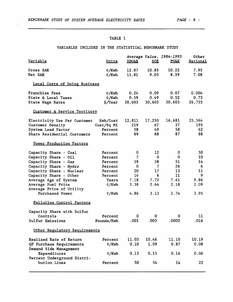
therefore NSAR. As seen in Table 1, California utilities have negligible coal

and oil generation capacity, whereas for the rest of the nation, coal and oil

together account for 60% of capacity.5 Gas capacity averages about 14%

nationally, but is over 50% for the three Califoria utilities. Nuclear power

is also used more intensively in California than in the rest of the nation.

Next we posit that the average age of a utility system affects NSAR. Because

of inflation, gross plant and depreciation expenses are higher for newer

systems, thereby increasing a utility's ratebase and raising its NSAR, other

things equal. We measure average system age by dividing total accumulated

depreciation by total depreciation expense. The three California utilities

have an average age varying from 7.18 to 7.72, more than two years less than

the average age of 9.86 years for the rest of our sample. Further, we expect

costs of fuel and purchased power to affect NSAR. We compute the average cost

of fuel as the sum of fossil, nuclear and other fuel costs divided by net

generation. The average fuel price is 3.38 C/Kwh for SDG&E, 2.64 for SCE and

2.18 for PG&E, while the national average is 2.09. We also calculate the

average cost of utility purchased power as total expenditures for utility


generated purchased power divided by megawatt hours purchased. SDG&E's

average price of utility purchased power is 4.86 C/Kwh compared to a rest of

nation average of 3.95, while that for SCE is 3.13 and PG&E is 2.74.

A third set of factors affecting NSARs comprises customer and service

territory factors. We expect that as use per customer declines, all else

equal, NSAR will increase because fixed costs will be spread over fewer sales.

The weather, customer mix and housing stock in California all contribute to

relatively low use per customer -- about one-half the national average. In

1984, for example, SDG&E ranked third, PG&E twelfth, and SCE fourteenth lowest

in the US in Kwh per customer; in 1993 the respective rankings were third,

seventh and ninth. Customer density -- the number of residential customers

per square mile -- may also influence costs. Given the added expense of

installing and maintaining complex distribution facilities and the higher

costs of obtaining right-of-ways, we expect that other things equal, urban

areas are more costly to serve. SCE and PG&E have much smaller customer

density than the national average (67 and 37 vs. 195), but that for SDG&E

(219) is slightly higher than the average. Customer composition, such as

residential customers as a percentage of total customers, can affect NSAR,

particularly when costs of distribution are large relative to transmission

services. 6 The size of this share for the three California utilities is

virtually the same as the national average -- 88%. A final customer and

service territory factor that can reasonably be expected to affect NSAR is the

system average load factor, calculated as the ratio of system average demand

to the system maximum or "peak" demand, both in megawatts. Since utilities

with lower load factors must allocate the cost of meeting peak demand across

fewer units, we expect that, ceteris paribus, system average load factor and

NSAR are negatively related. Load factors for the SDG&E and PG&E are close to

the national average (58% vs. 62%), but for SCE it is lower at 49%.


A fourth set of factors affecting NSAR reflects the cost of complying

with local, state and federal regulations concerning pollution abatement

standards. To estimate the effects of air pollution regulations on NSAR, we

attempted to obtain data on the amount of nitrogen oxide and sulfur dioxide

generated by various types of generation units, in pounds per Mwh; our

expectation was that such air pollution emissions would be inversely related

to NSAR. Although we were successful in obtaining suitable measures for

sulfur dioxide, we were unable to obtain reliable data for nitrogen oxide.

Thus, we employ sulfur dioxide emissions as a proxy variable for the total

emissions generated by the various types of generation units, and the

percentage of capacity with sulfur control as a measure of the added cost of

pollution controls. While sulfur controls affect 11% of the rest of the

nation's generation capacity, for the three California utilities this share is

zero. Not surprisingly, therefore, sulfur emissions are much smaller -- .001

pounds/Kwh for SDG&E, .003 for SCE, .0002 for PG&E -- than the .016 for the

rest of the nation.

The fifth set of factors affecting NSAR consists of other regulatory

requirements, most of which reflect compliance with state utilities'

commissions. The effects of qualifying facility purchase requirements, as

well as demand side management expenditures, are already accounted for by use

of the NSAR rather than the "gross" SAR; QF excess burdens are especially

large for SCE (1.09¢/Kwh) and PG&E (0.87) relative to the national average of

0.08C/Kwh. Two other regulatory policies are of particular interest. The

CPUC requires California investor-owned electric and telephone utilities to

convert a portion of their overhead distribution lines to underground

facilities, thereby incurring costs to install underground facilities in

already-developed areas, and to remove existing overhead lines. Some local

governments, for example San Diego, require additional underground

BENCHMARK STUDY OF SYSTEM AVERAGE ELECTRICITY RATES

TABLE 1

VARIABLES INCLUDED IN THE STATISTICAL BENCHMARK STUDY

Average Value, 1984-1993Units SDG&E SCE PG&EVariable

Gross SARNet SAR

C/KwhC/Kwh

Local Costs of Doing Business

Franchise FeesState & Local TaxesState Wage Rates

Customer & Service Territory

C/KwhC/Kwh

$/Year

12.8711.81

0.240.59

30,603

10.859.03

0.090.49

30,603

10.228.59

0.070.52

30,603

OtherNational

7.957.08

0.0040.73

26,755

Electricity Use Per CustomerCustomer DensitySystem Load FactorShare Residential Customers

Power Production Factors

Capacity Share - Coal

Capacity Share - Oil

Capacity Share - Gas

Capacity Share - HydroCapacity Share - NuclearCapacity Share - Other

Average Age of SystemAverage Fuel PriceAverage Price of Utility

Purchased Power

Pollution Control Factors

Capacity Share with SulfurControls

Sulfur Emissions

Kwh/Cust 12,811 17,250Cust/Sq Mi 219 67

Percent 58 49Percent 89 88

PercentPercentPercentPercentPercentPercentYearsC/Kwh

C/Kwh

PercentPounds/Kwh

0759

02014

7.183.38

4.86

0.001

12058

717

67.722.64

3.13

0.003

Other Regulatorv Reouirements

Realized Rate of ReturnQF Purchase RequirementsDemand Side Management

ExpendituresPercent Underground Distri-

bution Lines

PercentC/Kwh

C/Kwh

11.03 10.460.10 1.09

0.13 0.15

Percent 50 54

16,681375887

0051261311

7.612.18

2.74

0.0002

25,564195

6288

501014

611

99.862.09

3.95

11.016

11.100.87

0.16

10.190.08

0.06

PAGE - 8 -

14 22


distribution line conversion. We measure the effects of such regulatory

policies as the percent of total cable miles that is underground. While this

percent is 22% for the rest of the nation, for SDG&E it is 50% and for SCE it

is 54%. Finally, in rate case proceedings regulated utilities are assigned an

allowed rate of return. Ceteris paribus, it is reasonable to expect that the

greater the allowed rate of return, the higher the NSAR. Data on allowed rate

of return were not available, but data on average realized rates of return for

the three California utilities suggest allowed rates of return slightly above

the national average -- 11.03% for SDG&E, 10.46% for SCE, 11.10% for PG&E, and

10.19% for the rest of the nation.

The data sources used to construct the variables described above include

the Utility Data Institute's FERC Form 1 Database (containing annual financial

and other information filed at the FERC by major utilities), the Edison

Electric Institute's Electric Fuel Statistics (monthly data on the costs and

quality of fuels used in electric plants), the Edison Electric Institute's

Uniform Statistical Reports (voluntary filings by utilities containing

information describing company operations), the US Bureau of Labor Statistics

(Consumer Price Indexes), and the US Bureau of Economic Analysis (wages and

employment by state).

In Table 1 we list the variables to be used in our econometric analysis,

and also provide sample means of these variables for the three California

utilities and for the remainder of our national sample.

III. SPECIFICATION OF THE ECONOMETRIC MODEL

We now proceed with a discussion of the specification of our econometric

model. We first discuss issues of functional form, next we consider how to

deal with those variables which might not be entirely exogenous to current

utility management, and then we elaborate on how management effects can be

incorporated using an error components stochastic specification that reflects


a hybrid of fixed and random effect considerations. We consider alternative

procedures for estimating parameters in an error components framework, given

the fact that our panel data set is unbalanced, and that the maximum number of

times a utility is observed -- ten -- is rather small.

The dependent variable in our econometric model is the logarithm of the

NSAR -- hereafter denoted LNSAR (later we report results on use of NSAR rather

than its logarithmic transformation). We expect that relationships involving

some variables, for example, real state wage rates, use per customer, customer

density, real average fuel costs, real utility wholesale purchased power, and

system age are most likely to affect LNSAR in a proportional manner, and thus

we include as explanatory variables in our model the logarithmic transforma-

tions of these variables, which we denote as LRWAGE, LUPC, LCD, LRFUEL, LRWPP

and LAGE, respectively. Other explanatory variables are already in percent

form, and thus we include them without further transformation; these include

generation capacity shares for coal, oil, gas, hydro, nuclear and other

(largely, geothermal), named CAPC, CAPO, CAPG, CAPH, CAPN and CAPOTH),

respectively. 7 A realized rate of return variable (ROR) is also included, as

is a time trend.

While many of the explanatory variables are plausibly outside the

immediate control of utility management (e.g., state wage rates, generation

capacity, system age), several other variables might arguably reflect current

management influences. First, use per customer might reflect utility-specific

pricing and other conservation policies; to allow for this possibility, we

will report regression results with and without the LUPC variable

"instrumented", using the logarithm of weather cooling degree days as an

instrumental variable. A second possible endogenous variable is LRFUEL, the

utility real average fuel cost; here an appropriate instrumental variable is

the state-specific average fuel cost. The final variable that could reflect


current management influence is the rate of return measure. In principle, we

would prefer to employ an ex ante rate of return, since in rate hearings NSAR

is set so as to produce an expected rate of return. However, the ex ante rate

of return is unobservable. We explore two alternative ways of handling this

situation.

First, one feasible procedure involves formulating the relationship

between the ex post and ex ante rates of return (ROR) as follows. Let

RORex post - RORex ante + 6-shock + v (1)

where the ex post ROR is the sum of the allowed ex ante ROR plus factors that

"shock" this anticipated ROR, plus a random effect v. We postulate that the

shock is a function of the deviation of use per customer from trend, measured

as the residual from a utility-specific regression equation of LUPC on a time

counter. We then solve the above equation for the ex ante ROR in terms of the

ex post ROR and the demand shock, i.e.,

RORex ante - RORex post - 6*shock - v. (2)

We implement this formulation by including as regressors in the LNSAR equation

both the RORex post and the "shock" (deviation from trend) variable, which we

denote as DLUPC. Note that while we expect the coefficient on RORex post to

be positive, perhaps counterintuitively, this formulation implies that the

sign on the DLUPC variable should be negative.

A second possible procedure is to employ an instrumental variable, such

as the Moody bond rating for each of the utilities. However, it is not clear

how appropriate the Moody bond rating would be, for one could argue that

Moody's ratings reflect their judgment on utility management efficiency, and

thus the Moody rating would be a jointly determined rather than exogenous

variable. Nonetheless, in our empirical results, we will report findings

results on the use of Moody bond ratings as instruments.


We now turn to issues of stochastic specification for our econometric

model, which we simply write as

yit - a + f'xit + uit (3)

where y is the dependent variable, there are K regressors in x in addition to

the constant term, i - 1,...,Nt, and t - 1,...,Ti (in our unbalanced panel,

not all utilities are observed in all years, thus Nt varies by year and Ti

varies over utilities), and a and the K #'s are unknown parameters to be

estimated.

With panel data, a common specification is that the mean zero random

disturbance term uit is the sum of a mean zero utility-specific component vi

that is constant over time, and an independent mean zero component Cit, with

the strictly positive variances of these two components being a2 and a2 8

For our purposes, the interpretation of vi is very important.9 One can

re-write (3) by substituting in the component error and gathering terms. This

gives us

yit - (a + vi) + f'xit + Cit (4)

where (a + vi) can be envisaged as a random intercept in the LNSAR equation

that varies across utilities. Since vi has mean zero, it reflects the

difference in LNSAR for utility i from the national average, ceteris paribus.

If vi is positive (negative), the LNSAR of utility i is larger (smaller) than

the national average, holding fixed the other factors (the x's) affecting

LNSAR. We postulate that that vi reflects the effects of management decisions

of utility i on its LNSAR; we recognize, however, that the effects of other

omitted variables might also be captured by vi.

If the vi's of the three California utilities -- SDG&E, PG&E and SCE --

were insignificantly different from zero, ceteris paribus, then in this

framework we would conclude that once one controls for the various regional,

economic and regulatory factors, the management effects of the three


California utilities are no different from the national average. On the other

hand, if the vi's were found to be positive (negative) and significantly

different from zero, then one might infer that the management impacts of the

three California utilities result in a larger (smaller) NSAR than the national

average, having controlled for the various regional, economic and regulatory

factors.

With the above error components stochastic specification, the variance-

covariance matrix of disturbances is homoskedastic but non-diagonal (see, for

example, Greene [1993, ch. 16]). In particular, E(u t) - aU + a2 for

each i, but E(uituis) - a2 when s t. Under these assumptions, estimation of

parameters by ordinary least squares (OLS) is consistent but not efficient,

and traditional OLS-based estimates of the standard errors are biased.

Two methods have commonly been used to obtain consistent and efficient

estimates of a and P, and reliable estimates of their variances in this error

components specification; these are usually referred to as fixed and random

effects estimators. The random effects estimator employs a transformation

based on consistent (often, OLS) estimates of a2 and a2, denoted s2 and

s2, in which the x's and y are first transformed so that xj t xijt -

Wixij for each of the regressors, and yit " yit - oiYi, where

2 -1/2

s 2 + T.s2

L 1- [ 2:T 2 (5)

OLS is then performed on the transformed y* and x*, which now satisfy the

Gauss-Markov conditions for optimality of OLS. 10 In cases where the panel is

balanced (when Nt - N and Ti - T), and under the assumption of normality of

disturbances, iteration of this feasible generalized least squares procedure

has been shown to yield estimates that are numerically equivalent to maximum


likelihood estimation.11 Although our panel is unbalanced, iteration is

feasible, and thus we iterate the transformation process until changes from

one iteration to the next are insignificant.

An alternative estimation procedure, known as fixed effects, replaces

the common intercept term a + vi (whose expected value is a) with utility-

specific constant terms ai for each i, and then employs OLS estimation. There

are four important facts to note about this fixed effects estimator.

First, it is well-known that employing OLS with utility-specific

intercept terms yields estimates of the P's that are numerically equivalent to

subtracting the utility-specific means of each y and x variable from their

observed values, and then doing OLS on this deviation-from-utility mean-

transformed data.12

Second, use of such a deviation from mean estimation procedure results

in relying completely on the "within-utility" sample variance of the x's and

y's to estimate P (but not the ai) , and therefore results in 4 estimates that

entirely ignore the between-utility variance. In our context, this complete

reliance on within-utility variance could be somewhat detrimental, since as

noted earlier, about 78% of our sample variance in NSAR is across utilities,

and only 22% is within utilities over time. By contrast, the random effects

estimator employs both between and within variance in estimating the '6s.13

Note also that use of the fixed effects estimator requires the estimation of

an additional N-1 utility-specific parameters (almost 100 here) when compared

to the random effects specification.

Third, under traditional assumptions, the fixed and random effects

estimators are asymptotically equivalent. To understand this equivalence,

note from Eq. (5) that the fixed effects estimator is equivalent to setting wi

- i. Since s2 and s2 are both strictly positive, wi approaches unity with

increasing Ti, because the denominator in square brackets in Eq. (5) converges


to infinity. In our sample, while Nt is almost 100, Ti is never larger than

ten and sometimes is as small as one. Evidence from Monte Carlo studies,

presented in Baltagi [1981], suggests that in finite samples (in his case, Ti

- 10) the fixed effects estimators have much greater variance. Thus we

believe that caution should be exercised in using large sample assumptions for

Ti to rationalize results based on the fixed effects estimator.14

Fourth, in the fixed effects specification, the utility-specific

intercept terms can be interpreted as ai - a + vi . Since the sum of all

residuals from econometric estimation is zero, the utility-specific vi thus

essentially reflect the mean of that utility's residuals over its Ti

observations. If the mean of these Ti residuals is large and positive

(negative), then in this framework the impacts of management on LNSAR results

in higher (lower) rates than the average; but if the mean of these Ti

residuals is small and statistically insignificantly different from zero, then

there is no evidence supporting above- or below-average management impacts.

The above discussion on fixed and random effect estimators is based on

the assumption that none of the x's is correlated with the E's. If, for

example, simultaneous equations considerations suggest that use per customer

or average fuel price might be endogenous, then to obtain consistent

estimates, one would want to modify both the fixed and random effect

estimators, employing, for example, an instrumental variable approach.15

These econometric considerations suggest to us a hybrid approach in

estimating management effects on NSAR. Since inclusion of utility-specific

intercepts consumes valuable degrees of freedom, we will employ a compromise

of the fixed and random effects approaches, using a fixed effects (utility-

specific intercepts) specification for observations on the three California

utilities, and a parsimonious in parameters random effects specification for

observations on the remaining 96 non-California utilities in our sample.16


This hybrid specification allows us to test for the existence of a "California

effect", yet does not overly parameterize the model. To test whether there is

a "California effect" (in which, controlling for other factors, the California

utilities are examined for whether their NSARs differ from the national

average), we will test the joint null hypothesis that the three intercept

terms of SDG&E, PG&E and SCE are simultaneously equal to zero. We will,

however, also undertake a number of specification and diagnostic tests, and

assess whether estimates and inference concerning the existence of any

"California effect" are robust to alternative estimation methods.17

IV. ECONOMETRIC RESULTS

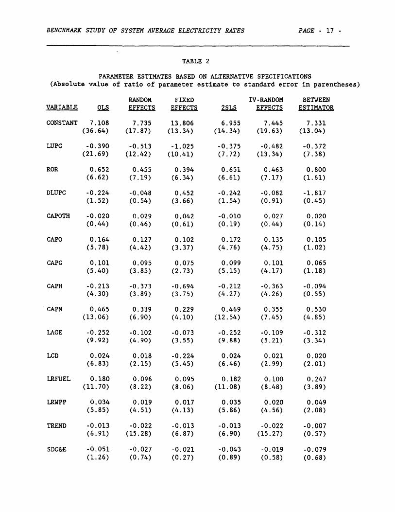
We begin with results from the most simple specification where we

estimate by OLS a model in which in addition to the explanatory variables

discussed above, the three California utilities have separate dummy variables;

results are given in the first column of Table 2. As is seen there, the

parameter estimates on the three California utilities are negative for SDG&E

and SCE, positive for PG&E, but the small t-values imply that each is

insignificantly different from zero. A joint F-test that the three California

utility coefficients are simultaneously equal to zero is not rejected -- the

test statistic is 1.12, while the 0.05 critical value is 2.60.

Several other results from this most basic model are also worth noting.

First, the estimate of the LUPC coefficient is -0.39 and significant, implying

that the elasticity of NSAR with respect to use per customer is about -0.4.

Second, while the impact of ROR on LNSAR is positive and significant as

expected, the coefficient on DLUPC (deviation from trend) is negative, as

expected, although not very reliably so. Third, coefficient estimates on the

generation capacity variables (interpreted as relative to coal) are

signfiicantly positive for oil, gas and nuclear, and negative for hydro.


TABLE 2

PARAMETER ESTIMATES BASED ON ALTERNATIVE SPECIFICATIONS(Absolute value of ratio of parameter estimate to standard error in parentheses)

RANDOM FIXEDEFFECTS EFFECTS 2SLS

IV-RANDOMEFFECTS

BETWEENESTIMATOR

CONSTANT 7.108 7.735(36.64) (17.87)

LUPC

ROR

DLUPC

-0.390 -0.513(21.69) (12.42)

0.652(6.62)

-0.224(1.52)

CAPOTH -0.020(0.44)

CAPO

CAPG

CAPH

CAPN

LAGE

LCD

LRFUEL

LRWPP

TREND

SDG&E

0.164(5.78)

0.101(5.40)

-0.213(4.30)

0.465(13.06)

-0.252(9.92)

0.024(6.83)

0.180(11.70)

0.034(5.85)

-0.013(6.91)

-0.051(1.26)

0.455(7.19)

-0.048(0.54)

0.029(0.46)

0.127(4.42)

0.095(3.85)

-0.373(3.89)

0.339(6.90)

-0.102(4.90)

0.018(2.15)

0.096(8.22)

0.019(4.51)

-0.022(15.28)

-0.027(0.74)

VARIABLE OLS

13.806(13.34)

-1.025(10.41)

0.394(6.34)

0.452(3.66)

0.042(0.61)

0.102(3.37)

0.075(2.73)

-0.694(3.75)

0.229(4.10)

-0.073(3.55)

-0.224(5.45)

0.095(8.06)

0.017(4.13)

-0.013(6.87)

-0.021(0.27)

6.955(14.34)

-0.375(7.72)

0.651(6.61)

-0.242(1.54)

-0.010(0.19)

0.172(4.76)

0.099(5.15)

-0.212(4.27)

0.469(12.54)

-0.252(9.88)

0.024(6.46)

0.182(11.08)

0.035(5.86)

-0.013(6.90)

-0.043(0.89)

7.445(19.63)

-0.482(13.34)

0.463(7.17)

-0.082(0.91)

0.027(0.44)

0.135(4.75)

0.101(4.17)

-0.363(4.26)

0.355(7.45)

-0.109(5.21)

0.021(2.99)

0.100(8.48)

0.020(4.56)

-0.022(15.27)

-0.019(0.58)

7.331(13.04)

-0.372(7.38)

0.800(1.61)

-1.817(0.45)

0.020(0.14)

0.105(1.02)

0.065(1.18)

-0.094(0.55)

0.530(4.85)

-0.312(3.34)

0.020(2.01)

0.247(3.89)

0.049(2.08)

-0.007(0.57)

-0.079(0.68)

PAGE - 17 -


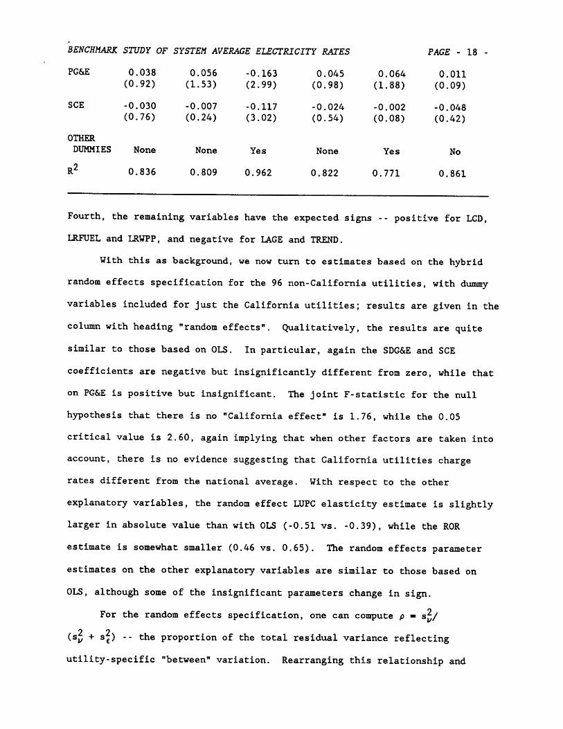
PG&E 0.038 0.056 -0.163 0.045 0.064 0.011(0.92) (1.53) (2.99) (0.98) (1.88) (0.09)

SCE -0.030 -0.007 -0.117 -0.024 -0.002 -0.048(0.76) (0.24) (3.02) (0.54) (0.08) (0.42)

OTHERDUMMIES None None Yes None Yes No

R2 0.836 0.809 0.962 0.822 0.771 0.861

Fourth, the remaining variables have the expected signs -- positive for LCD,

LRFUEL and LRWPP, and negative for LAGE and TREND.

With this as background, we now turn to estimates based on the hybrid

random effects specification for the 96 non-California utilities, with dummy

variables included for just the California utilities; results are given in the

column with heading "random effects". Qualitatively, the results are quite

similar to those based on OLS. In particular, again the SDG&E and SCE

coefficients are negative but insignificantly different from zero, while that

on PG&E is positive but insignificant. The joint F-statistic for the null

hypothesis that there is no "California effect" is 1.76, while the 0.05

critical value is 2.60, again implying that when other factors are taken into

account, there is no evidence suggesting that California utilities charge

rates different from the national average. With respect to the other

explanatory variables, the random effect LUPC elasticity estimate is slightly

larger in absolute value than with OLS (-0.51 vs. -0.39), while the ROR

estimate is somewhat smaller (0.46 vs. 0.65). The random effects parameter

estimates on the other explanatory variables are similar to those based on

OLS, although some of the insignificant parameters change in sign.

For the random effects specification, one can compute p = s2Y

(s2 + s ) -- the proportion of the total residual variance reflecting

utility-specific "between" variation. Rearranging this relationship and


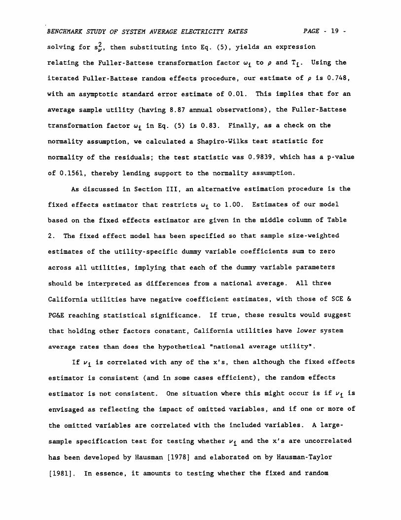
solving for s2, then substituting into Eq. (5), yields an expression

relating the Fuller-Battese transformation factor wi to p and Ti. Using the

iterated Fuller-Battese random effects procedure, our estimate of p is 0.748,

with an asymptotic standard error estimate of 0.01. This implies that for an

average sample utility (having 8.87 annual observations), the Fuller-Battese

transformation factor wi in Eq. (5) is 0.83. Finally, as a check on the

normality assumption, we calculated a Shapiro-Wilks test statistic for

normality of the residuals; the test statistic was 0.9839, which has a p-value

of 0.1561, thereby lending support to the normality assumption.

As discussed in Section III, an alternative estimation procedure is the

fixed effects estimator that restricts wi to 1.00. Estimates of our model

based on the fixed effects estimator are given in the middle column of Table

2. The fixed effect model has been specified so that sample size-weighted

estimates of the utility-specific dummy variable coefficients sum to zero

across all utilities, implying that each of the dummy variable parameters

should be interpreted as differences from a national average. All three

California utilities have negative coefficient estimates, with those of SCE &

PG&E reaching statistical significance. If true, these results would suggest

that holding other factors constant, California utilities have lower system

average rates than does the hypothetical "national average utility".

If vi is correlated with any of the x's, then although the fixed effects

estimator is consistent (and in some cases efficient), the random effects

estimator is not consistent. One situation where this might occur is if vi is

envisaged as reflecting the impact of omitted variables, and if one or more of

the omitted variables are correlated with the included variables. A large-

sample specification test for testing whether vi and the x's are uncorrelated

has been developed by Hausman [1978] and elaborated on by Hausman-Taylor

[1981]. In essence, it amounts to testing whether the fixed and random


effects estimators yield estimates of the P's that are statistically

insignificantly different from each other. Although results from such a

Hausman test suggest a statistically significant difference between the fixed

and random effects estimates at better than the 5% level, thereby favoring the

fixed effects estimator, the fixed effects results appear less plausible on

economic grounds.

For example, the fixed effect estimated elasticity of system average

rate with respect to use per customer is -1.025 -- an estimate we believe is

unrealistically large given the substantial fraction of a typical utility's

variable costs in its total costs. Also, rather than having the expected

negative sign, the estimated coefficient on DLUPC in the fixed effects model

is positive and significant; similarly, while one expects customer density to

have a positive impact on system average rate, the fixed effect parameter

estimate on LCD is negative and significant.

An alternative consistent estimator when vi is correlated with one of

the regressors involves use of an instrumental variable (IV) procedure. Given

the large observed difference between the fixed and random effect coefficient

on LUPC, we focus particular attention on the possible correlation of vi with

LUPC. We therefore re-estimate the OLS and random effect models with LUPC

"instrumented" using the logarithm of cooling degree days. Results are given

in columns 4 and 5, respectively, of Table 2. Again we obtain the robust

finding that none of the California utilities has a significant positive

coefficient estimate; for both 2SLS and IV-Random Effects, the SDG&E and SCE

effect estimates are negative and insignificant, while that for PG&E is

positive but insignificant. Moreover, the IV-Random Effects estimates on the

model's explanatory variables are very similar to the random effects estimates

that do not take the possible correlation of vi and LUPC into account.18 The


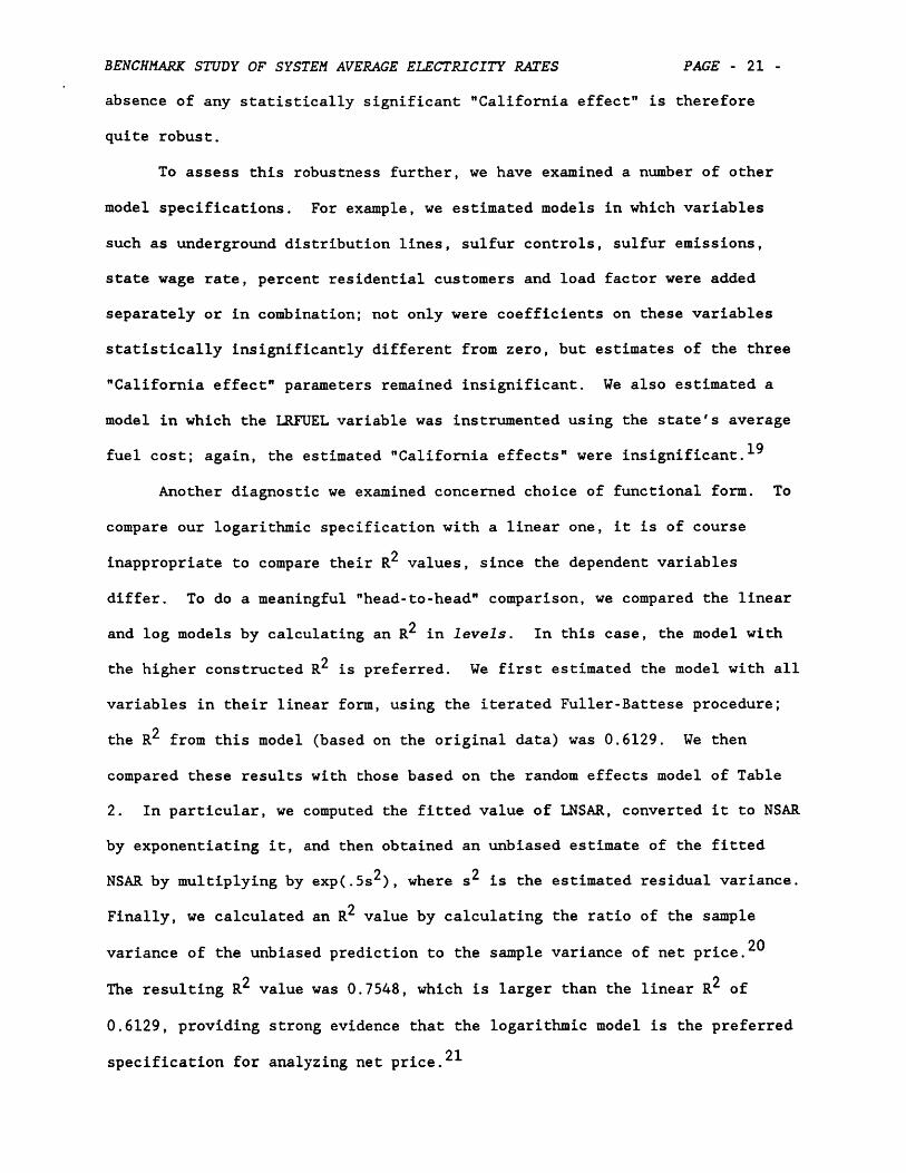
absence of any statistically significant "California effect" is therefore

quite robust.

To assess this robustness further, we have examined a number of other

model specifications. For example, we estimated models in which variables

such as underground distribution lines, sulfur controls, sulfur emissions,

state wage rate, percent residential customers and load factor were added

separately or in combination; not only were coefficients on these variables

statistically insignificantly different from zero, but estimates of the three

"California effect" parameters remained insignificant. We also estimated a

model in which the LRFUEL variable was instrumented using the state's average

fuel cost; again, the estimated "California effects" were insignificant. 19

Another diagnostic we examined concerned choice of functional form. To

compare our logarithmic specification with a linear one, it is of course

inappropriate to compare their R2 values, since the dependent variables

differ. To do a meaningful "head-to-head" comparison, we compared the linear

and log models by calculating an R2 in levels. In this case, the model with

the higher constructed R2 is preferred. We first estimated the model with all

variables in their linear form, using the iterated Fuller-Battese procedure;

the R2 from this model (based on the original data) was 0.6129. We then

compared these results with those based on the random effects model of Table

2. In particular, we computed the fitted value of LNSAR, converted it to NSAR

by exponentiating it, and then obtained an unbiased estimate of the fitted

NSAR by multiplying by exp(.5s 2), where s2 is the estimated residual variance.

Finally, we calculated an R2 value by calculating the ratio of the sample

variance of the unbiased prediction to the sample variance of net price. 20

The resulting R2 value was 0.7548, which is larger than the linear R2 of

0.6129, providing strong evidence that the logarithmic model is the preferred

specification for analyzing net price. 21


Yet another check on robustness involves use of what is commonly called

a "between" estimator. It is of course well-known that in balanced panels the

random effects estimator is a weighted average of the fixed effect "within"

estimator and a between estimator, where the between estimation involves

computing sample means of all variables for each utility, and then (in our

context) running a regression of each utility's mean LNSAR on the sample means

of the explanatory variables.22 This suggests the following mental exercise.

Suppose one collects sample means over 1984-93 annual observations of the

left- and right-hand variables for each of the 96 non-California utilities,

and then runs an OLS regression. Given the resulting parameter estimates

based on only the non-California utilities, use the sample means of the

explanatory variables for SDG&E, SCE and PG&E to generate predicted LNSARs for

these utilities, and then prediction errors by subtracting the predicted LNSAR

from the three utilities' mean actual LNSAR. Then test whether these

prediction errors are statistically significantly different from zero.

The above exercise is numerically equivalent to running the same between

regression, but adding dummy variables for each of the three California

utilities, including these utilities in the estimation, and then testing

whether the dummy variable coefficients for the three utilities are

statistically significantly different from zero.23 Results from such an

exercise are given in the final column of Table 2. As is seen there, again

one finds that the estimated California effects for SDG&E and SCE are negative

and insignificant, while that for PG&E is positive but insignificant. We

conclude, therefore, that once one controls for various regional, economic and

regulatory factors, there is no evidence supporting the notion that the

performance of California utilities is worse than the national average

benchmark.


V. IMPLICATIONS AND INTERPRETATION OF FINDINGS

The results reported in the previous section are surprisingly robust.

The common theme of these results is that once one controls for various

regional, economic and regulatory factors outside the direct and immediate

control of utility management, system average rates charged by the California

utilities are not statistically different from the national average. An

important issue raised by these results, however, concerns the interpretation

of why it is that the unadjusted rates are so much higher in California than

in the rest of the country. What insights can our estimated model provide in

helping us understand what accounts for California's higher unadjusted system

average rates?

One way of interpreting California's relatively high rates is to proceed

as follows. Suppose a California utility had values of the various regional,

economic and regulatory variables equal to those of the national average. In

such a hypothetical case, what would that California utility's system average

rate be, and how much of the difference between its actual and hypothetical

rates could be attributed to each of the various explanatory variables?

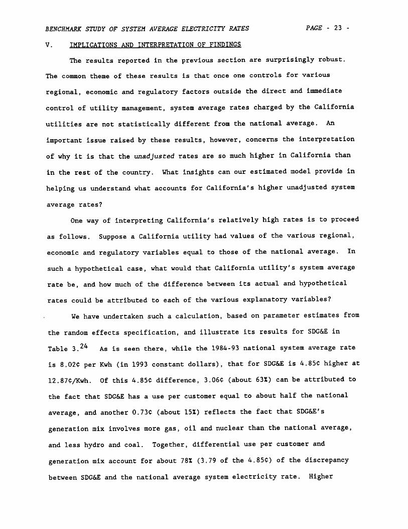
We have undertaken such a calculation, based on parameter estimates from

the random effects specification, and illustrate its results for SDG&E in

Table 3.24 As is seen there, while the 1984-93 national system average rate

is 8.02C per Kwh (in 1993 constant dollars), that for SDG&E is 4.85C higher at

12.870/Kwh. Of this 4.85U difference, 3.06¢ (about 63%) can be attributed to

the fact that SDG&E has a use per customer equal to about half the national

average, and another 0.73C (about 15%) reflects the fact that SDG&E's

generation mix involves more gas, oil and nuclear than the national average,

and less hydro and coal. Together, differential use per customer and

generation mix account for about 78% (3.79 of the 4.85t) of the discrepancy

between SDG&E and the national average system electricity rate. Higher


TABLE 3

DECOMPOSING THE SDG&E AVERAGE ELECTRICITY PRICE DIFFERENCEFROM THE NATIONAL AVERAGE

Average Electricity Price (1984-93)(C/Kwh in 1993 constant dollars)

SDG&E 12.87National Average 8.02Difference 4.85

Decomposition of the Difference

C/Kwh

Lower Electricity Use per Customer 3.06Generation Mix 0.73Higher Average Fuel Price 0.41Younger Age of System 0.25Higher Franchise Fees 0.24Higher Customer Density 0.19Higher Demand-Side Management Expenditures 0.07Higher Cost of Utility Purchased Power 0.06Time Trend 0.04Higher Rate of Return 0.03Expenditures for QF Power 0.00Lower State and Local Taxes -0.14Remaining Influence of the Above Factors

Not Separately Measurable 0.12SDG&E Effect (Not Statistically Significant) -0.21

TOTAL 4.85

% Difference

63.1%15.18.55.24.93.91.41.20.80.60.0-2.9

2.5-4.3

100.0%

average fuel price, younger age of system, higher franchise fees, and higher

customer density together account for another 1.09( (about 22%) of the

difference, while the remaining factors essentially cancel one another out.25

Finally, note that the SDG&E effect -- the effect of SDG&E management on

system average rate -- is slightly negative, -0.21C/Kwh -- implying that

ceteris paribus, SDG&E's prices are slightly lower than the national average.

From a statistical standpoint, however, this estimated SDG&E effect is not

reliably different from zero.

PAGE - 24 -


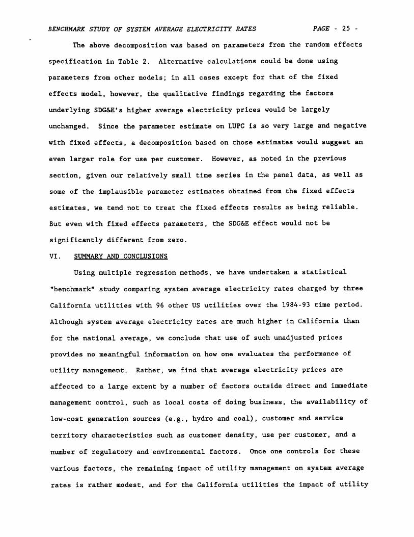
The above decomposition was based on parameters from the random effects

specification in Table 2. Alternative calculations could be done using

parameters from other models; in all cases except for that of the fixed

effects model, however, the qualitative findings regarding the factors

underlying SDG&E's higher average electricity prices would be largely

unchanged. Since the parameter estimate on LUPC is so very large and negative

with fixed effects, a decomposition based on those estimates would suggest an

even larger role for use per customer. However, as noted in the previous

section, given our relatively small time series in the panel data, as well as

some of the implausible parameter estimates obtained from the fixed effects

estimates, we tend not to treat the fixed effects results as being reliable.

But even with fixed effects parameters, the SDG&E effect would not be

significantly different from zero.

VI. SUMMARY AND CONCLUSIONS

Using multiple regression methods, we have undertaken a statistical

"benchmark" study comparing system average electricity rates charged by three

California utilities with 96 other US utilities over the 1984-93 time period.

Although system average electricity rates are much higher in California than

for the national average, we conclude that use of such unadjusted prices

provides no meaningful information on how one evaluates the performance of

utility management. Rather, we find that average electricity prices are

affected to a large extent by a number of factors outside direct and immediate

management control, such as local costs of doing business, the availability of

low-cost generation sources (e.g., hydro and coal), customer and service

territory characteristics such as customer density, use per customer, and a

number of regulatory and environmental factors. Once one controls for these

various factors, the remaining impact of utility management on system average

rates is rather modest, and for the California utilities the impact of utility


management (relative to the national average) is insignificantly different

from zero. This finding of no difference in prices, holding constant the

effects of factors outside of California utilities' control, is robust, being

sustained in a large number of alternative models and estimation methods.

It would of course be desirable to decompose further the reasons for

differences in system average rates. One possible line of research could

examine distinct cost categories such as generation, transmission and

distribution, or even a further disaggregation of these functions. Although

of great interest, such a study would impose very challenging difficulties to

any empirical researcher. The most obvious difficulty is the problem of

obtaining reliable time series of disaggregated cost data that is comparable

across utilities. The accounting procedures by which utilities allocate fixed

and common costs to functional activities vary even between the all-electric

utilities, are considerably more complex and idiosyncratic for combined gas-

electric utilities, and probably have varied over time for all utilities as

well. It is worth emphasizing that in capital-intensive industries such as

electric utilities, how one measures fixed costs presents important

difficulties, and we suspect that reliable conclusions that are robust to

alternative accounting conventions would be difficult to obtain.

There are, however, a number of useful extensions of this research.

Within the electric utility context, one might also want to take into account

variations in the "quality" of electricity, such as the system reliability and

average duration of any downtime. 26 More generally, the approach taken in

this paper could in principle be applied to other industries, not only

partially regulated ones such as natural gas and telecommunications, but also

to firms in various deregulated industries.


FOOTNOTES

iThe methodology of our "bottom line" statistical benchmark study differs ofcourse from benchmark studies that focus on a much more disaggregated,detailed and homogeneous operational or functional level of analysis.

2We selected the 1984-93 time period since public data were not generallyavailable in electronic format prior to 1984.

3We employ the BLS regional CPIs for the Northeast, South, North Central andWest. Although the BLS publishes CPIs for selected metropolitan areas, themetropolitan CPIs do not cover all utilities in our sample; moreover, the BLSadvises that the metropolitan-level data may not be as reliable as theregional data. It is worth noting that use of a regional CPI capturesdifferential rates of price change across regions, but it does not incorporateregional differentials in price levels.

4Since all investor-owned utilities face the same federal statutory tax ratesand provisions, we do not net out federal tax payments.

5The coal capacity indicated for SCE reflects partial ownership of coalgeneration facilities in Arizona. There is no coal generation capacity withinCalifornia.

6Industrial users often receive services from high-voltage transmission lines,whereas residential users require service from low-voltage distribution linesthat transform power to levels acceptable for home use. Thus it is reasonableto posit that NSAR and share of residential customers are positively related.

7Since these percentages sum to 100% for each utility each year, they are notindependent; we drop the coal share, and thus regression coefficients shouldbe interpreted as relative to coal.

8For the moment, assume that E(vivj) - 0 for i7 j, E(Eitejs) - 0 for sft orifj, and that E(eituj ) - 0 for all i, t and j.

9Our interpretation of this error component model builds on the work of Hoch[1955], Mundlak [1961] and Griliches [1957]. These writers were particularlyinterested in obtaining estimates of the #'s (in their contexts, typicallyestimates of Cobb-Douglas production function parameters based on farm outputsand inputs data) that were not biased because of a failure to take managementimpacts into account. While these researchers focussed on consistentestimates of the P's, here we use their approach but instead focus more of ourattention on obtaining consistent estimates of the management effects. For areview of this literature, see Chamberlain [1984].

10This transformation is due to Wayne Fuller and George Battese [1973,1974].

110n this, see Badi Baltagi and Qi Li [1992], and Trevor Breusch [1987].Notice that the traditional concept of a likelihood function whose samplemagnitude is to be maximized becomes quite unclear when the panel isunbalanced, since the disturbance vector has random length.

12 See, for example, Greene [1993, Chapter 16].

13For a clear exposition of this point, see Yair Mundlak [1978].

PAGE - 27 -


14Results of Monte Carlo studies have also been reported in Baltaji-Rak [1992]and Taylor [1980], but all these studies typically focus their attention onsmall sample estimates of the P's, not of the ai's.

15A discussion of estimation issues for error components models in the contextof simultaneous equations is found in, inter alia, Baltagi-Raj [1992, pp.91-94].

16To do this, we employ the Fuller-Battese transformation for all observationsother than those involving the three California utilities, and introduceindicator variables for the three California utilities, whose data are nottransformed with the Fuller-Battese procedure.

17We also considered employing a more time-series oriented stochasticspecification, such as one involving an ARMA process. While feasible in thecontext of balanced panels (see, for example, Galbraith and Zinde-Walsh[1995]), in our situation with missing observations and an unbalanced panel,there would be a very substantial decrease in the number of observationsavailable for efficient estimation.

18It is worth noting that the weather cooling degree days variable performsvery well as an instrument; its t-value in the first-stage regression was11.72.

19We also undertook an analysis in which we instrumented the ROR variableusing Moody's bond rating categories. Although this increased the size of thecoefficient on the ROR variable, again each of the dummy variable coefficientson the three California utilities was insignificantly different from zero(point estimates for SDG&E and SCE were negative, while that for PG&E waspositive).20For a discussion, see fn. 16, p. 144 in Berndt [1991], which in turn is

based on Aitchison and Brown [1966].

21It is worth noting that with the linear specification, occasionally some ofthe California utilities had a positive and significant "California" effect.Such findings are not reliable, however, since the linear specification isclearly dominated by the logarithmic model.

22See Green [1993, Chapter 16] for details and references.

23This occurs since the fitted and actual values are identical (the residualis zero) when each additional parameter is unique to the additional utilityobservation. For discussion, see Berndt [1991, Exercise 7, pp. 48-50]. Itshould also be noted that in the context of an unbalanced panel such as ours,both equations are estimated weighting each utility by Ti.

24To do this with a logarithmic specification, one must allocate the linearand joint multiplicative effects on price, and compute partial effects byevaluating at the sample means of the other variables. This involves use ofTaylor's series approximations. Details of the procedures we employed aregiven in a technical appendix available from the authors upon request.

25The non-zero impact of time trend reflects the fact that data for all threeCalifornia utilities were available for the entire ten-year time period,whereas the "average utility" was observed 8.87 years.

26For analyses of reliability in the electric utility industry, see, inter

PAGE - 28 -


alia, Doane, Hartman and Woo [1988a,b], Grosfeld-Nir and Tishler [1993], andWoo and Train [1989].

PAGE - 29 -


REFERENCES

Aitchison, John and James A. C. Brown (1966], The Lognormal Distribution,Cambridge, England: Cambridge University Press.

Baltagi, Badi [1995], The Econometric Analysis of Panel Data, - get reference

Baltagi, Badi H. [1981], "An Experimental Study of Alternative Testing andEstimation Procedures in a Two-Way Error Component Model," Journal ofEconometrics, Vol. 17, No. 1, September, 21-49.

Baltagi, Badi and Qi Li [1992], "A Monotonic Property for Iterative GLS in theTwo-Way Random Effects Model," Journal of Econometrics, Vol. 53, No. 1-3, July-September, 45-51.

Baltagi, Badi H. and Baldev Raj [1992], "A Survey of Recent TheoreticalDevelopments in the Econometrics of Panel Data," in Baldev Raj and BadiH. Baltagi, eds., Panel Data Analysis, Heidelberg: Physica-VerlagHeidelberg, 85-109.

Berndt, Ernst R. [1991], The Practice of Econometrics, Reading, MA: Addison-Wesley Publishers, Inc. *

Biorn, Erik [1992], "The Bias of Some Estimators for Panel Data Models withMeasurement Errors," in Baldev Raj and Badi H. Baltagi, eds., Panel DataAnalysis, Heidelberg: Physica-Verlag Heidelberg, 51-66.

Breusch, Trevor S. [1987], "Maximum Likelihood Estimation of Random EffectsModel," Journal of Econometrics, Vol. 36, 383-389.

Chamberlain, Gary [1984], "Panel Data," in Zvi Griliches and Michael D.Intriligator, eds., Handbook of Econometrics, Vol. II, Amsterdam: North-Holland, 1247-1318.

Chamberlain, Gary [1982], "Multivariate Regression Models for Panel Data,"Journal of Econometrics, Vol. 18, 5-46.

Doane, Michael, Raymond Hartman and Chi-keung Woo [1988a], "HouseholdPreferences for Interruptible Rate Options and the Revealed Value ofService Reliability," The Energy Journal, Special Electricity 0

Reliability Issue, Vol. 9, pp. 121-134.

Doane, Michael, Raymond Hartman and Chi-keung Woo [1988b], "Households'Perceived Value of Service Reliability: An Analysis of ContingentValuation Data," The Energy Journal, Special Electricity ReliabilityIssue, Vol. 9, pp. 135-150.

Fuller, Wayne A. and George E. Battese [1973], "Transformations for Estimationof Linear Models with Nested Error Structure," Journal of the AmericanStatistical Association, Vol. 68, 636-642.

Fuller, Wayne A. and George E. Battese [1974], "Estimation of Linear Modelswith Cross-Error Structure," Journal of Econometrics, Vol. 2, No. 1,May, 67-78.


Galbraith, John W., and Victoria Zinde-Walsh [1995], "Transforming the Error-Components Model for Estimation with General ARMA Disturbances," Journalof Econometrics, Vol. 66, No. 1, 349-355.

Greene, William H. [1993], Econometric Analysis, Second Edition, New York:MacMillan.

Griliches, Zvi [1957], "Specification Bias in Estimates of ProductionFunctions," Journal of Farm Economics, Vol. 39, 8-20.

Grosfeld-Nir, Abraham and Asher Tishler [1993], "A Stochastic Model for theMeasurement of Electricity Outage Costs,". The Energy Journal, Vol. 14,No. 2, 157-174.

Hausman, Jerry A. [1978], "Specification Tests in Econometrics, Econometrica,Vol. 46, pp. 1251-1271.

Hausman, Jerry A. and William E. Taylor [1981], "Panel Data and UnobservableIndividual Effects," Econometrica, Vol. 49, 1377-1398.

Hoch, Irving [1955], "Estimation of Production Functions and Testing forEfficiency," Econometrica (abstract), Vol. 23, No. 3, July, 325-326.

Hsiao, Cheng [1986], Analysis of Panel Data, Cambridge: Cambridge UniversityPress.

Mundlak, Yair [1978], "On the Pooling of Time Series and Cross Section Data,"Econometrica, Vol. 46, No. 1, January, 69-85.

Mundlak, Yair [1961], "Empirical Production Functions Free of ManagementBias," Journal of Farm Economics, Vol. 43, 44-56.

Taylor, William E. [1980], "Small Sample Considerations in Estimation fromPanel Data," Journal of Econometrics, Vol. 13, No. 2, June, 203-223.

Woo, Chi-keung and Kenneth Train [1989], "The Cost of Electric PowerInterruptions to Commercial Customers," The Energy Journal, SpecialElectricity Reliability Issue, Vol. 9, 161-172.

PAGE - 31 -

investor-owned a mit-ceepr 95-005wp june

Documents