investor networks in the stock market -...

Investor Networks in the Stock Market∗

Han Ozsoylev† Johan Walden‡ M. Deniz Yavuz§ Recep Bildik¶

August 23, 2013

∗We thank seminar participants at the 2012 meetings of the American Finance Association, the Berkeley finance lunchseminar, the Berkeley-Stanford seminar, HKUST, the 2011 Indiana State Conference, the 2011 Mini-Conference on Networksand the Global Economy at Brown University, Johns Hopkins University, the Swedish Institute for Financial Research (SIFR),University of Minnesota, University of Miami, and UT Austin. The Department of Information Technology at UppsalaUniversity, and especially Per Lotstedt have been tremendously supportive. Thanks to Niclas Eriksson and Ludvig Larruyat the same department for excellent research assistance with the program implementation and computational analysis of thedata, and also to Andreas Kieri, Joakim Saltin, and Shiraz Farouq for continuing their work. We also thank Mehmet IhsanCanayaz for research assistance on news collection and Sabanci University School of Management for their hospitality whilepart of this work was carried out. We are grateful to John Beshears, Jonathan Cohn, Jennifer Conrad, Nicolae Garleanu,Simon Gervais, Joel Hasbrouck, Craig Holden, Peter Jones, Ron Kaniel, Shimon Kogan, Christine Parlour, Raghu Rau,Mark Seasholes, Sheridan Titman, Laura Veldkamp and Jeffrey Zwiebel for valuable comments and suggestions, and toAaron Clauset for providing us with code for the community algorithm. We thank Gil Shallom for developing the initialcode. Finally, we thank the Editor, David Hirshleifer, and a referee for very valuable comments and suggestions.

†Said Business School, University of Oxford, and College of Administrative Sciences and Economics, Koc University,E-mail: [email protected]

‡Corresponding author: Haas School of Business, University of California at Berkeley, 545 Student Services Building#1900, CA 94720-1900. E-mail: [email protected], Phone: +1-510-643-0547. Fax: +1-510-643-1420. Supportfrom the Institute for Pure and Applied Mathematics (IPAM) at UCLA is gratefully acknowledged.

§Purdue University, Krannert School of Management, 403 West State Street, West Lafayette, IN 47907. E-mail: [email protected]

¶Istanbul Stock Exchange. E-mail: [email protected]

1

Investor Networks in the Stock Market

Abstract

We study the trading behavior of investors in an entire stock market. Using an

account level dataset of all trades on the Istanbul Stock Exchange in 2005, we identify

traders with similar trading behavior as linked in an empirical investor network (EIN).

Consistent with the theory of information networks, we find that central investors earn

higher returns and trade earlier than peripheral investors with respect to information

events. Overall, our results support the view that information diffusion among the

investor population influences trading behavior and returns.

2

1 Introduction

What determines the heterogeneous trading behavior and performance of individual investors in the stock

market? One motive for heterogeneous trading is that investors have diverse information, allowing well-

informed investors to outperform those who are less informed (Hellwig (1980); Grossman and Stiglitz

(1980); Kyle (1985)). In this paper, we focus on such diverse information as a motive for heterogeneous

trading, and study investor behavior through the lens of information networks (Colla and Mele (2010),

Ozsoylev and Walden (2011), Han and Yang (2013)). Loosely speaking, an information network describes

how diverse information signals diffuse over time among a population of investors. Investors who are

centrally placed in such a network tend to receive information signals early, whereas investors who are in

the periphery tend to receive them later. As a result, the trading behavior and profitability of individual

investors are influenced by their position in the network, and the dynamics of aggregate asset prices

depend on the network’s general topological properties.

Identifying the underlying information network in the entire stock market is of course a major chal-

lenge. Our first contribution in this paper is to develop a method to proxy for the market’s information

network, using observable data. The general idea is that information links may be identified from realized

trades, since traders who are directly linked in the network will tend to trade in the same direction in

the same stock at a similar point in time, say on the same day or even within an hour of each other.

By focusing on such short time periods we aim to capture information that is diffused into the market

over a relatively short horizon, say about a week. Using this approach, we identify an Empirical Investor

Network (EIN), and in simulations show that the true information network is indeed well estimated by

the EIN. This approach may also be applied to partial data. For example, in simulations we show that

when only one third of the agents in a network are included in a reduced network (corresponding to in-

cluding about 10% of the links in the full network), the correlation between true centrality and centrality

calculated in the reduced network is about 0.5.

We calculate the EIN using account level trading data that covers all trades on the Istanbul Stock

Exchange (in Turkey) in 2005. We first verify that the EIN is fairly stable over time. We test the stability

3

by dividing our sample period into two six month sub-periods and define an EIN for each of these periods.

The overlap between the two EINs is strongly significantly different from the overlap of two randomly

generated networks. We also verify that some investors systematically trade before their neighbors, and

that such early trading is positively related to centrality. Together, these results support the view that

the EIN captures information diffusion. This provides our second contribution.

We study the relationship between investor centrality and returns, and find substantial support for a

positive relationship. In our multivariate regressions, a one-standard deviation increase in centrality, all

else equal, leads to a 0.7%-1.8% increase in returns (over a 30-day period) depending on the specification.

These results are obtained after controlling for other variables such as trading volume, so the tests

distinguish investors who are central in the information network from investors who just trade a lot.

Documenting the positive relationship between centrality and returns is our third contribution.

Finally, as a fourth contribution, we document that centrality is directly related to acting early on

information. We identify several idiosyncratic information events that were associated with large stock

price movements, and find that central investors in the network tended to trade—in the right direction—

before peripheral investors. We also verify that when central investors’ trades were delayed by one day,

their excess performance decreased by close to 30%, and that returns to central investors were higher in

months with a relatively large number of earnings announcements. All these results are consistent with

information diffusion, with central agents gaining early access to information.

Our results suggest that information diffusion is an important determinant of investors’ trading be-

havior and profitability. Specifically, our results have two components: First that our network captures

information diffusion and, second, that the network is consistent with a decentralized diffusion mecha-

nism, as opposed to diffusion through public media channels. However, there is also the possibility that

omitted variables, alternative trading motives, or purely mechanical relationships between variables may

generate similar results. In several additional analyses and robustness tests, we find further support for

the information diffusion story over such alternative explanations.

Any alternative explanation of the first component must be consistent with several facts: First, it

4

should generate a network that is stable over time. Second, it should be consistent with the trading

behavior of investors over the short time periods that the network is based upon. Third, it should lead

to a positive relationship between centrality and returns over 1-3-month horizons. Fourth, it should lead

to a positive relationship between centrality and trading early with respect to information events in the

market. Several alternative explanations fail at least one of these properties. For example, various style-

related explanations broadly defined, e.g., correlated wealth shocks or momentum strategies, may satisfy

the first property, but typically not the second, third and fourth.1 Similar arguments make it implausible

that various biases (e.g, home bias) explain the results. Finally, the first, third and fourth properties make

price impact, e.g., because of illiquidity, an unlikely explanation. We discuss this extensively throughout

the paper.

For the second component, our results are not as conclusive but we do find some evidence in support

of a decentralized diffusion mechanism, consistent with, e.g.,word-of-mouth communication and Internet

discussion boards, but not with diffusion through public media channels. First, we verify that the network

is consistent with a decentralized structure. The median number of direct links for an investor is 159,

within the range of what is documented in the literature on social networks. More importantly, the

number of communities in the network, defined as groups of investors who are tightly connected among

themselves but only sparsely connected to other investors, identified by a standard algorithm (Closet,

Newman, and Moore (2004)) is 1,109—much higher than what we would expect if major news media

provided the main diffusion channel. Second, we study the timing of trading activity with respect to

when an information event was reported in media. We find that most of the increased trading activity

occurred before the event was reported, again inconsistent with media as the main diffusion channel.

We also carry out several variations of the tests to show robustness and to rule out mechanical relations

between variables as a driver of the results. We do out-of-sample tests, constructing the centrality measure

in the first six months of the trading period, and verifying that the measure is positively related to profits

1Standard investment “styles” are, e.g., defined in Brown and Goetzmann (1997) and Barberis and Shleifer (2003). Thereis also a large literature that explains heterogeneous portfolio holdings with hedging motives (see, e.g., Mayers (1973); Bodie,Merton, and Samuelson (1992); Massa and Simonov (2006); Parlour and Walden (2011), Betermeier, Jansson, Parlour, andWalden (2012)). Also, heterogeneous preferences, e.g., different risk aversion, induce trading. We include such tradingmotives in our broad definition of “investment styles.”

5

and to trading early with respect to information events in the following six months. We vary window

lengths and several other parameters, exclude links between investors in the same brokerage house, and

use alternative profit measures, all with very similar results. Finally, to rule out explanations related

to the higher sophistication of institutional investors, we run the tests with these investors excluded,

with virtually identical results. This, for example, mitigates the likelihood that our results are due to

automated high-frequency trading algorithms, since we would expect to mainly find such algorithms

among the institutional investor population. Thus, in total our results provide substantial support for

decentralized information diffusion among the investor population, although we cannot completely rule

out alternative explanations.

Our paper belongs to the literature on heterogeneous information, networks, and trading in stock

markets. There is extensive evidence of frequent communication among stock market investors, and this

evidence suggests that investors exchange information about the stocks that they trade. Shiller and

Pound (1989) vividly demonstrates this: the authors survey 131 institutional investors in the NYSE and

ask them what prompted their most recent stock purchase or sale. The majority asserts that it was

their discussions with their peers. Ivkovic and Weisbenner (2007) find similar evidence for households,

and Hong, Kubik, and Stein (2004) provide further evidence that fund managers’ portfolio choices are

influenced by word-of-mouth communication.2 Our paper is also related to the literature that studies the

relationship between news, investor behavior and stock returns, e.g., Tetlock (2007) and Tetlock (2010).

Our study contributes to the literature by providing — to the best of our knowledge — the first market-

wide study of information diffusion in a stock market, and its effects on the entire investor population’s

behavior and trading profits.

Our study reinforces a view of the stock market as a place where information is incorporated into asset

prices through gradual decentralized diffusion. Information networks provide an intermediate information

2Other studies provide indirect evidence that communication between investors affect their trading behavior. Feng andSeasholes (2004) find that Chinese trades are highly correlated when divided geographically, consistent with local communi-cation among investors. Cohen, Frazzini, and Malloy (2008) posit that communication via shared education networks allowsfund managers to earn abnormal returns (see also Das and Sisk (2005), Fracassi (2012) and Pareek (2012)). Shive (2010)develops an epidemic model of investor behavior that predicts individual investor trading. Duffie, Malamud, and Manso(2009) develop a dynamic equilibrium search model, in which information diffusion occurs when agents with heterogeneousinformation meet randomly.

6

channel, in between the public arena where news events and prices themselves make some information

available to all investors, and the completely local arena of private signals and inside information. Such

a view is consistent with the presence of significant stock market movements unaccompanied by public

news events, as studied in Cutler, Poterba, and Summers (1989) and Fair (2002), and with substantially

varying stock market returns and trading volume over time, as analyzed in Gabaix, Gopikrishnan, Plerou,

and Stanley (2003).

2 Framework

We introduce a simple model of information diffusion in a stock market, to describe the concept of an

information network, and to understand how an information network may be identified from observed

trading behavior.

2.1 Trading in an information network

Let us for simplicity study a network structure according to Figure 1, in which there are NI = 21 investors

in an information network, as an example. Each node (circle) represents an agent (investor, trader), and

each edge (line) represents a direct link between two agents, i.e., that the two agents are connected. In

other words, linked agents are neighbors in the network. These connections are bidirectional, i.e., if agent

i is connected to agent j, then j is connected to i. For technical reasons, we always assume that an agent

is connected to himself.

In addition to the agents in the network, we assume that there is a large number, NU of uninformed

noise traders, whose trading motives we do not model and who randomly take on opposite sides of trades.

Altogether there are N = NI +NU traders in the model.

[Figure 1 about here.]

Trading occurs at discrete times, t = 0, 1, 2, . . .. At each point in time, each of the NI agents in the

network receives a distinct signal about stocks in the market, i.e., agent i receives signal sti at time t. We

denote the set of signals agent i’ has received at time t by Iti , and it then follows that st

′i ∈ It

i for t′ ≤ t.

7

For simplicity, we assume that only one signal in each time period, agent nt’s signal, is valuable. Thus,

at time t, agent nt receives a signal and trades. All the other signals at time t are worthless, the other

agents understand this, and therefore do not trade. The expected profits from agent nt’s trade is positive.

We assume that there is a noise trader willing to take the opposite position in the trade, whereas agents

in the information network only trade when they receive information.

Now, agent nt may “share” his signal with one of his neighbors between t and t+ 1. Specifically, for

each of his neighbors, there is a probability of q1 that agent nt shares his information. For example, given

the network in Figure 1, if agent 1 received the initial signal, then for each of agents 2, 3, 4, and 5, the

probability is q1 that he will share it with that agent. Given that information is shared, a receiving agent

— let us call him n2t — then trades at t+1, however his expected trading profit is lower than that of agent

1, in line with the assumption that, as time passes, the expected profits from trading on the information

declines. This could, e.g., be because agent nt has already traded and some of his information is already

incorporated into prices. The signal may also be slowly diffusing into the market through other channels.

We thus have that stnt∈ It+1

n2t. In a similar manner, agent n2

t shares his signal between t+ 1 and t + 2,

with probability q2, to each of his neighbors, who then trade at t + 2 and realize even lower expected

profits than agent n2t . At t+ 3, the signal is completely incorporated into the stock market’s prices and

no further profits can be made.3

A general network of N agents can be represented by a neighborhood (adjacency) matrix, E ∈

{0, 1}N×N , with Eij = 1 if investors i and j are directly connected, and Eij = 0 otherwise.4 The

bidirectionality of connections implies that E is symmetric (i.e., Eij = Eji for all i and j). Symmetric

information sharing arises naturally in the theory of information networks (see, e.g., Ozsoylev and Walden

(2011), Han and Yang (2013), and Walden (2012)), since both agents need to share information in a

relationship for information sharing to be mutually beneficial. Intuitively, with a one-sided relationship,

an agent who only transmits information to another agent but never receives information from that agent

3It would of course be easy to extend the model to longer sequences of information diffusion, as well as trading incontinuous time.

4We use the following matrix notations: A matrix is defined by the [·] operator on scalars, e.g., E = [eij ]ij . We write(E)ij for the scalar in the ith row and jth column of the matrix E , or, if there can be no confusion, we write it as Eij .

8

has no incentive to participate in the relationship.

We use the convention that the first NI agents are the ones in the information network, and the

remaining NU are the noise traders (each of which is only connected to himself). The matrix representa-

tion of the network in Figure 1, is given in Figure 2 below, where it is assumed that there are NU = 29

noise traders, so that the total number of traders is N = 21 + 29 = 50. In the figure, dots represent

connections, i.e., elements for which Eij = 1. The upper left part of the matrix represents the agents in

the network, EI . For example, focusing on the first row, the five first elements are nonzero, showing that

agent 1 is connected to himself, and agents 2-5, respectively. The lower right part of the matrix (elements

22-50) is diagonal, representing the unconnected noise traders.


We are now in a position to formally define a general information network, given an information

diffusion mechanism among agents:

Definition 1 Consider a population of agents among which heterogeneous information signals, sti, diffuse

over time. Then E defines the information network of signals available to the population over time, if for

all agents i, j and times t, t′, the probability that sti ∈ It′j is

• zero when dE (i, j) > t′ − t,

• greater than zero when dE(i, j) ≤ t′ − t.

Here, dE(i, j) denotes the distance between agents i and j in the network E, i.e., the length of the shortest

path between the two agents, where we use the convention that dE (i, j) = ∞ if there is no path between

the two agents.

It is easy to check that given the information diffusion mechanism between agents just described, the

information network is indeed the one shown in Figure 1.

We define the degree of investor i as the investor’s number of neighbors, including himself, Di = |{j :

Eij = 1}|.

9

2.2 Centrality and profits

Intuitively, investor 1 in Figure 1 seems to be well-positioned to make high profits. Although investors

2-5 have more direct neighbors, investor 1 is within a distance of two from all the other investors, in

contrast to the other agents, and will therefore receive many valuable signals. In other words, investor 1

is more central than the other investors and is therefore expected to have higher trading profits (Ozsoylev

and Walden (2011)).

There are several measures of centrality. Common measures include degree, eigenvector, Katz, and

closeness centrality (see, e.g., Friedkin (1991)). Eigenvector and Katz centrality are closely related;

eigenvector centrality can be viewed as a limit case of Katz centrality. As shown in Valente, Coronges,

Lakon, and Costenbader (2008), these measures of centrality are typically strongly correlated in real-world

networks.

We prefer to use eigenvector centrality as our measure for two reasons. The first reason is computa-

tional. It is relatively easy to compute in a large-scale network. Measures like closeness centrality, on the

other hand, require keeping track of higher order paths between nodes, which is simply not feasible given

the size of our network.5 The second reason is theoretical. Walden (2012) shows that the information

advantage—i.e., the advantage an investor has because of his position in the network, that allows him

to earn excess returns—is closely related to eigenvector centrality, but less so to other measures, e.g.,

closeness centrality.

The intuition for why eigenvector centrality works well is simple. In an information diffusion model,

eigenvector centrality captures the fundamental properties of what makes an agent well-positioned in the

network, namely how much information he receives and how delayed the information is. This is easiest

seen by observing that one way to calculate eigenvector centrality is by using so-called power iterations.

Specifically, eigenvector centrality is a sum of powers of the degree matrix—in other words basically a sum

of degrees of different orders. The higher the order, the more signals reaches an investor, but the more

5To calculate closeness and betweenness centrality, powers of the neighborhood matrix, Em, need to be calculated (orsome variant thereof), which is a major task if N is large. The reason is that even though E is a sparse object, Em ismuch less sparse, leading to severe memory and CPU requirements. In contrast, the largest eigenvector can be calculatedefficiently, using just E .

10

delayed these signals are. A measure that perfectly reflects information advantage needs to re-weight the

importance of different orders of degree somewhat, but eigenvector centrality captures the spirit of the

two fundamental properties.

A vector C where the ith element represents agent i’s (eigenvector) centrality is constructed as follows.

Let Ci denote the centrality of investor i. By letting i’s centrality score be proportional to the sum of

the scores of all the investor’s neighbors, we derive

Ci =1

λ

∑

j

EijCj, or in vector form C =1

λEC. (1)

The proportionality constant, λ, is an eigenvalue of E and C is the corresponding eigenvector. The

eigenvector corresponding to the largest eigenvalue is the centrality vector.6 For large matrices, power

iterations provide an efficient way of solving (1).7

A closely related measure that we use is rescaled centrality, C/D, i.e., the ratio between centrality and

degree. This measure may be more robust in capturing information advantage than pure centrality in an

empirically estimated investor network. The reason is that when there are noise traders who trade a lot

for alternative reasons, these traders typically also end up with many links in the empirically estimated

investor network. This, in turn, increases their centrality, although they do not have an information

advantage. Their rescaled centrality will typically be low though, as it should be since these traders are

not central in the information network.

In our empirical tests, our dataset contains the full population of traders in the market. If someone

wanted to use our methodology to estimate centrality in other datasets, however, there may be omitted

agents in those datasets and an important question is therefore how robust the centrality measure is to

omitting some agents. Specifically, given a network with N agents, assume that a centrality measure

6The neighborhood matrix, E , has only nonnegative elements. It therefore follows from the Perron-Frobenius theoremthat it has a real maximal eigenvalue, and that the associated eigenvector has only nonnegative elements. This is thecentrality vector. The only potential issue is uniqueness, since E may not be irreducible, but this has not caused a problemin our tests.

7Specifically, given an estimate of the centrality vector, Ck, an updated estimate is obtained by performing the iterationCk+1 = 1

‖Ck‖ECk, where ‖Ck‖ is some suitable chosen normalization of Ck (e.g., the mean-square norm). If E contains

relatively few non-zero elements—in other words, if the matrix is sparse—and the largest eigenvalue is significantly largerthan the second largest eigenvalue, then each iteration can be calculated quickly and convergence to the true centralityvector is obtained in few iterations.

11

is calculated using only a subset of the network, with n < N of agents. How closely related is this

approximated centrality measure to true centrality among these n agents? To study this question, we

simulate a large number of networks. We then randomly exclude a fraction of agents, and calculate a

“reduced” centrality of the remaining n agents, based on the reduced network. To see how well true

centrality (based on the network with N agents) is approximated by reduced centrality (based on the

subnetwork with n < N agents), we plot the average correlation between the two measures, while varying

n.

The results are shown in Figure 3, using a network size of N = 500 agents. We see that the average

correlation (the vertical axis) is a smooth function that slowly decreases as n (on the horizontal axis)

decreases. When only one third of agents (about 170) are “kept,” the average correlation is about 0.5.

This is quite remarkable, given that only about 10% (1/32) of the links remain in the reduced network.

Even with only 20% of the agents in the reduced network (100 agents, with about 1/52 = 4% of the

original links), the average correlation is still about 0.35. We have verified that the results are scalable

in the size of the network, by varying N . We conclude that the centrality measure is quite robust to

omitting a significant fraction of agents.

The randomness and independence of excluded agents is a parsimonious assumption. For instance,

if the researcher is interested in measuring the relative centrality of agents within a community (defined

as a tightly connected cluster of investors that have fewer connections with investors outside of the

community), excluding the network outside of the community may be even less of an issue. On the

contrary, systematically excluding central agents in a network may potentially increase the problem. We

leave the study of such questions for future research.


2.3 Estimating the neighborhood matrix

In practice the information network is not observable, but since agents who are connected in the network

will tend to trade in similar stocks in the same direction at similar points in time, we can identify an

12

empirical proxy for the true network — an Empirical Investor Network (EIN).

A fairly straightforward approach for small networks would be to use maximum likelihood estimation.

The EIN would be identified as the network for which the observed trades were most likely. For larger

networks, however, simpler approximations are needed. As discussed in Gomez-Rodriguez, Leskovec, and

Krause (2012), exact maximum likelihood estimation is not feasible for large networks because the number

of possible networks grows super-exponentially with the number of nodes, making an exact approach

computationally infeasible. Gomez-Rodriguez, Leskovec, and Krause (2012) study infection contagion

in a network, and the problem of identifying a network from observed contagions. They develop an

approximation method that is computationally feasible for networks with up to several thousand nodes.

However, since our network is a couple of orders of magnitude larger than what is computationally feasible

with their method and, furthermore, our inference problem differs from theirs, we choose an even further

simplified approach.

Definition 2 The Empirical Investor Network, EΔt,M , in a stock market which operates over some finite

time period, is defined such that for each pair of investors, i, j �= i, EΔt,M = 1 if and only if agents i and

j traded in the same stock in the same direction within a time window of Δt at least M times over the

full time period.

The EIN can be computed efficiently even for networks with hundreds of thousands (or even millions)

of investors, as long as the Δt window is not too large. In our tests we will vary Δt between a minute and

a day. Intuitively, the EIN captures information diffusion by linking investors who trade close in time.8

Furthermore, it is straightforward to show (see the Internet Appendix) that the EIN can be viewed as

an approximation of the network one would obtain through maximum likelihood estimation:

Proposition 1 Consider an information network, EI , in which each agent, after receiving a signal,

immediately trades, and then shares the signal with probability q > 0 per unit time within the next Δt

time interval, with each of his neighbors. For small Δt, given a realization of trades between 0 and T , the

8Note that our definition of EIN is different from the one taken in Adamic, Brunetti, Harris, and Krilenko (2010), whoidentify two investors as connected if they traded with each other. Such traders are on the opposite side and will thus notbe viewed as connected in our model.

13

EIN EΔt,1I is a maximum likelihood estimator of the true underlying information network. Specifically, it

is the unique maximum likelihood estimator that minimizes the total number of links in the information

network.

Thus, for small Δt, the EIN is indeed a maximum likelihood estimator, and it is also consistent with a

sparse network in that it minimizes the number of links. The intuition behind the result is that for short

time windows, the likelihood of information diffusion is relatively low and the likelihood of observing a

sequence of trades will therefore be higher if links are formed between any two agents for which diffusion

may have occurred. The EIN will therefore be the maximum likelihood estimator. For longer windows,

the EIN will be an approximation because of the tradeoff between the increased likelihood of observing an

immediate trade when adding a link to the network, and the decreased likelihood such a link introduces

of not observing a trade in the future. For sparse networks, we would usually expect the former effect

to dominate, and the EIN should therefore provide a good approximation for sparse networks even with

relatively longer time windows. We next show that the EIN indeed performs well in simulations for such

networks.

2.4 Performance of estimation method

In this section, we focus on the case where the threshold for a connection is M = 1, and the time period

is one unit of time, so that agents who trade within the period [t, t + 1] for some t are connected, i.e.,

we focus on E1,1. We simulate trades in the network in Figure 1 with N = 100 agents, over 50 trading

periods, with probabilities q1 = 0.25, q2 = 0.5 (defined in Section 2.1). We choose a higher per-agent

probability for information diffusion at the second stage, since it seems natural to assume that agents

are pickier in who they share information with early on, when information is more proprietary.

An example of a realized EIN is shown in Figure 4. We see that the general structure of the true

network is identified, although not every link is correct. For example, in the upper left part of the EIN,

which represents the agents in the information network, there are several elements just off the diagonal

that are nonzero, representing links between agents, although no such links exist in the true information

14

network. This is, for example the case for agents 20 and 21, who are incorrectly linked in the EIN.

The reason is that agent 3 received a signal that he shared with agents 20 and 21, who then traded

simultaneously and who were thereby falsely identified as directly linked, although they are in practice

only indirectly linked through their common connection with agent 3. Similarly, erroneous links occur

in the part of the matrix with uninformed agents. These links arise when two agents happen to take

the opposite position of their informed counterparties, at similar points in time. In the informed part of

the network matrix (the first NI ×NI in the upper left corner), there are 42 agents, who are incorrectly

identified as being linked. Also, there are 4 agents who are actually linked, but who are not estimated to

be linked. Thus, in total, 46 elements are misclassified, corresponding to about 10% of the total number

(441) of elements of EI . In the noise trader part of the network, there are 126 incorrect links, scattered

randomly, corresponding to about 2% of the total number of elements (6,241). Thus, overall the number

of misclassified elements is low. The EIN also captures the true centrality of agents in the network well.

The average correlation between the centrality vector of the true network and that of the EIN is 0.64.


We verify that the method is scalable, i.e., that the fractions of misclassified elements does not blow

up when the size of the network increases, and also that the method works for more general network

structures. To do this, we simulate a large number of networks of N agents, where NI = 0.2N agents

are in the information network, and the remaining agents are noise traders, NU = 0.8N . We randomly

generate links between investors in the information network. To keep the network sparse, a property that

is known to hold for large-scale networks in practice and in this context is consistent with the view that

investors on average are only directly connected to a small part of the rest of the population, we choose

the probability for a link to be such that the expected number of links of each agent in the information

network is√NI . Thus, in an information network of size 100 each agent is on average connected to 10%

(10/100) of the rest of the population, whereas in a network of size 250,000 each agent is on average

connected to about 0.2% (500/250,000). As we shall see, this is of the same order of magnitude as in the

networks we will study.

15

We simulate NI paths of trading in each randomly generated network, and calculate the average

fraction of misclassified elements over many randomly generated networks. By varying N , we verify that

the fraction of misclassified elements does not grow with the size of the network. For N = 200, the total

fraction of misclassified links is 0.23%, and the fraction of misclassified links in the information network

(excluding the NU noise traders) is 2.0%. With N = 2000 agents, the fraction of misclassified links is

slightly lower: 0.20% of the total links and 1.6% for the information network. Thus, the identification

method is scalable.

To summarize, the EIN is scalable, an exact maximum likelihood estimator for short time windows,

and performs well in simulations. We will therefore use it in our empirical tests.

2.5 Limitations and additional analysis

The EIN can be estimated from account level data on trades, but there are limitations to solely relying

on the EIN. We discuss these limitations and additional analyses and tests that can be used to obtain

further insight about the role of information diffusion in the market. We will carry out these tests in

subsequent sections.

Omitted variables and alternative trading motives may potentially generate an empirically estimated

network similar to the one driven by information diffusion. However, any alternative explanation needs to

satisfy several additional properties, in addition to generating correlated trades among investors. First,

it needs to lead to a positive relationship between centrality and profitability in the 1-3 month horizon,

which is the profit horizon we will use in our tests. Second, it should be consistent with investors’

trading behavior over short horizons. Specifically, we will mainly use a time window of 30 minutes

when constructing the EIN. Under information diffusion, central agents systematically trade before their

peripheral neighbors within this time horizon, and an alternative explanation should also have this

property. Third, if the EIN represents links in an information network, it will be relatively stable over

time. By comparing EIN’s constructed over different time periods, such stability may be verified. A

fourth test is based on actual information events. Given a set of information events identified in the

media that moved stock prices, central agents in the EIN should tend to trade earlier with respect to

16

these events than peripheral agents. Such a test provides a direct link between centrality and information,

and therefore efficiently separates information diffusion from other explanations. These predictions and

associated tests will allow us to fairly confidently conclude that EIN captures information diffusion,

although we cannot completely rule out all alternative explanations.

The EIN does not directly identify the underlying channels of information diffusion. Two such chan-

nels may be word-of-mouth communication between investors, and Internet discussion boards. These are

examples of fairly decentralized diffusion mechanisms. An alternative channel would be diffusion through

different public media outlets, where some investors get their information earlier than others, e.g., from

national news broadcasts as opposed to local newspapers. This corresponds to a centralized diffusion

mechanism, with a few information hubs.9 We propose two approaches to gain additional insight about

the underlying channels of diffusion. First, we can measure how centralized the EIN is, using standard

methods. Three natural measures are the median number of connections investors have, the so-called

network centralization index, and the number of local communities in the network, defined as groups of

investors who are tightly connected among themselves but only sparsely connected to other investors. A

low median number of neighbors and centralization index is consistent with a decentralized network, as is

a high number of communities. This, in turn, goes against public media as the main source of diffusion.

The second approach uses the information events. By studying the increased trading activity around

these events, insight about the diffusion channels can be obtained. Specifically, if the bulk of the increase

in trading activity occurs before the event is reported in the news, this goes against public media as

the main channel of diffusion. We will use these tests to better understand the underlying information

diffusion channel.

The EIN alone will not be able to determine whether the information being diffused is about funda-

mentals or about something else. As described in Ozsoylev and Walden (2011), information diffusion can

be incorporated into a noisy rational expectations model. In such a model, asset prices are based on fun-

9Of course, these different channels have the common property that information is gradually incorporated into agents’trading behavior and asset prices, in line with our results. In its most general form, an information network describesinformation available to agents in their trading decisions over time, as expressed in Definition 1, regardless of the channelthrough which information diffusion occurs.

17

damentals, and are semi-strong form efficient in that they reflect all public information. However, there

may also be information, not about fundamentals, but, e.g., about investor sentiment and, furthermore,

prices are not necessarily efficient. Some of the information could even be that central agents know that

peripheral agents will follow suite shortly in their trades, although our tests in Section 4.4 will show that

other types of information events are also important.

Finally, our approach is based on a rational framework with information diffusion, in which central

agents have information advantage, but additional network mechanisms could also be relevant. For exam-

ple, agents could suffer from persuasion bias or other biases, imposing costs of centrality; see DeMarzo,

Vayanos, and Zwiebel (2003), Han and Hirshleifer (2012) and Heimer and Simon (2012). Furthermore,

it could be that agents with many links need to invest more time in upholding these links, and therefore

have less time to invest in their own information acquisition. The latter mechanism would punish direct

links to other investors, but still reward higher-order links, again along the lines of our main theme that

centrality is valuable.

3 Description of the data

3.1 The Istanbul Stock Exchange

The Istanbul Stock Exchange (ISE) was founded as an autonomous, professional organization in early

1986. The ISE is the only corporation in Turkey established to provide trading in equities, bonds and

bills, revenue-sharing certificates, private sector bonds, foreign securities and real estate certificates as

well as international securities. All ISE members are incorporated banks and brokerage houses. There

were exactly 100 ISE members in 2005.

The ISE is an order-driven, multiple-price, continuous auction market with no dedicated market

makers or specialists. A computerized system automatically matches buy and sell orders on a price and

time priority basis. The buyers and sellers enter the orders through their workstations located at the ISE

building and also in their headquarters. It is a blind order system with trading ISE members identified

upon matching. The system enables members to execute several types of orders such as “limit,” “limit

18

value,” “fill or kill,” “special limit,” and “good till date” type orders. Members can enter buy and sell

orders with various validity periods of up to one trading day. Unmatched orders without a specific validity

period are canceled at the end of the trading session.

The stock trading activities are carried out on workdays in two separate sessions, 9:30-12:00 for the

first session and 14:00-16:30 for the second session. Settlement of securities traded in the ISE is realized

by the ISE Settlement and Custody Bank Inc. (Takasbank), which is the sole and exclusive central

depository in Turkey. Turkey has a liberal foreign exchange regime with a fully convertible currency. In

2005, the value of one Turkish Lira (TL) varied between 0.7-0.8 USD. Since August 1989, the Turkish

stock and bond markets have been open to foreign investors without any restrictions on the repatriation

of capital and profits. At the start of our sample period, the vast majority (94.7%) of the institutional

investors in our sample were foreigners.

ISE ranks 19th across the world with market capitalization of 201 billion dollars in 2005 (Source:

World Development Indicators). The average daily trading volume ranged between approximately USD

300 and 700 million. The turnover ratio of the ISE was 155% in 2005, which was comparable to the

turnover ratio of %129 for the US. There is only one time zone in Turkey.

3.2 The data

Our dataset contains all the trades on the ISE over a 12 month period, January 1-December 31, 2005.

During this period there were 303 stocks actively traded in the market. In the data, each trader is

identified by a unique account number, and for each trade the following information is available: time of

trade, stock ticker, number of shares traded, price, account number of purchaser and seller, purchaser and

seller types (private, institutional or brokerage house trading on its on own account), and whether the

trade was a short sale. In total there were 580,142 active accounts during the time period. Of these, 489

were classified as institutional accounts and the remaining 579,653 were classified as individual accounts.

On average about 200,000 trades were executed on a day when the ISE was open.

19

3.3 The Empirical Investor Network

We calculate the EIN for the market, using the threshold M = 3, and varying the length of the time

window, Δt, between 1 minute and 30 minutes. We will subsequently extend the time window to a

whole day, and also vary the threshold M between 1 and 10. By using a window length of no more

than one day, we separate information driven “fast” trading from other types of trading such as portfolio

rebalancing, momentum investing, style investing etc., which we typically think of as occurring over lower

trading frequencies. For example, momentum strategies are typically implemented over a 3-month to 1-

year horizon, and the impact of value and size strategies are rarely studied over shorter than monthly

horizons. In contrast, the EIN is constructed to capture information diffusion effects at horizons of about

a week taking higher order effects into account (i.e., degrees of order higher than one). For computational

reasons, we use shorter time windows for several analyses.10

In Table 1, we provide summary statistics for the EIN, using window lengths between 1 minute and

half an hour. Overall the network is very sparse. Even with the 30-minute time window, investors are on

average only connected to a small fraction, 0.3% (1,781/580,142), of the population. This may still seem

like a large number. With a narrow interpretation of network connectedness representing communication

between investors in a social network, one may expect the number of links to be in the low hundreds, not

in the thousands. For example, Ugander, Karrer, Backstrom, and Marlow (2011) find that the average

Facebook user in the U.S. had 214 friends, and about one per mil of the users have 5,000 friends (the

maximum number allowed by Facebook), as of May 2011. Hampton, Goulet, Rainie, and Purcell (2011)

report a similar number. They survey 2,255 American adults on their use of social networking sites and

their overall social networks. In their sample, the average Facebook user has 229 friends. They also

find that the average American adult has an overall network of 634 social ties, including weak ties, e.g.,

acquaintances. Dunbar (1992) proposes 150 as being a natural size of social groups. With a stricter

definition of social ties, e.g., only including family, close friends, and colleagues, one may expect an even

10This is justified since it turns out that the structure of the EIN is very similar across different length, as are our mainresults. This is not surprising since two investors who are directly linked when a window length of ΔT is chosen, are typicallyalso indirectly connected (at a higher degree than one) with a window length ΔT ′ < ΔT . The main difference when varyingthe windows length is that we find a somewhat stronger relationship between centrality and profitability for longer windows.

20

lower number, say less than 50. Internet discussion boards about stocks as channels for information

diffusion on the other hand may bring the number higher, perhaps even above 1,000.

The mean number of links in our network is relatively high. However, our distribution is severely

skewed, caused by the small fraction of investors with a very large number of links. The most connected

investor when the 30-minute window length is used has over two hundred thousands links, and is thereby

directly connected to almost half of the other investors. We suspect that these investors are (unofficial)

market makers that provide liquidity—an investor group that is not part of our theoretical model—and

therefore come out as extremely connected, although they are not part of the information network. We

will eliminate the undo influence of such extreme observations by truncating the distribution and by

using logs of variables. In Figure 5, we show the cumulative distribution of number of investor links.

We see that 90% of investors have less than 4,000 links. The median number of links thus seems more

informative than the mean. The median number of links with the 30-minute window is 159, which is

within the lower range of numbers mentioned in the literature.

A related measure is the number of communities in the network. Briefly, a set of investors who are

heavily connected among themselves, but sparsely connected with other investors, form a community. In

a decentralized information diffusion process, e.g., representing diffusion through social ties, we would

expect a large number—many hundreds or even thousands—of relatively small communities in the net-

work. With a more centralized diffusion process on the other hand, we would expect a smaller number

of communities. For example, if the network represents information diffusion through different media

channels, we would typically expect the number of communities to be less than a hundred.11

We estimate the number of communities, using the method developed in Closet, Newman, and Moore

(2004). This is one of the few methods that can be used for a network of our size; see also Newman

(2004). For computational reasons, we exclude the 10% most connected investors. This also helps us

avoid influence from outliers. The algorithm detects 1,109 communities of average size 523, consistent

with decentralized information diffusion, but not with centralized diffusion, e.g., through news media.

11There were 4 TV news channels and 28 newspapers with an average daily circulation over 10,000 in Turkey in 2005(source: www.medyatava.com).

21

A third measure of network centralization is the network centralization index, NCI, which is a number

between 0 and 100% that measures how centralized a network is compared with a completely centralized

star network, see Freeman (1979). Such a star network has the maximal NCI of 100%. The NCI for our

EIN is 4.5%. This is quite low. For example, in a network with many local communities where each

community has a star structure, an NCI of 4.5% corresponds to having about 1,250 such communities

with about 460 investors in each, again higher than what we would expect from diffusion through public

media channels.

In total, the structure of our EIN is thus consistent with decentralized information diffusion through

social ties, Internet discussion boards, and local communities rather than through public media.

[Table 1 about here.]


3.4 Trading volume, number of trades, and returns

For each investor i and trade z we define number of shares traded (Niz), trading price (Piz) and trading

quantity (Qiz = Niz ∗ Piz). We first construct a vector of total trading quantity, Qi, where Qi =∑

z Qiz

is the total value (in TL) of purchases and sales that investor i executes over the full time period (1 year).

Similarly, we define the vector of number of trades of each individual investor, Ni, over the total time

period. We also define the log-counterparts, qi and ni, i.e., vectors with qi = log(Qi) and ni = log(Ni).

To measure trading returns, we use the same approach as in in Barber, Lee, Liu, and Odean (2009),

but focus on individual investors’ trades rather than on investor groups. Briefly, we define a window

length, ΔT which we set to 30 days but vary for robustness purposes later. For each trade, z, the realized

return is

μiz = sign ∗ P t+ΔT − P t

P t,

where P t+ΔT is the closing price of the stock 30 days after the trade (or, if the market is closed on

that day, the closing price the nearest open day after), P t is the price at which the stock was traded and

the sign indicates the direction of the trade, and is negative for an investor on the sell side of a trade

22

and positive for an investor on the buy side of a trade. Here, P is corrected for stock splits, and takes

dividend payments into account. We then define the return of the investor from all trades as the value

weighted average returns from all trades within a year,12

μi =

∑z μiz ∗Qiz∑

z Qiz. (2)

We use the value weighted return measure μi in our main tests. In robustness tests, we verify that the

results are very similar when using average returns instead, i.e., when weighing each transaction equally

in determining an investor’s profitability.

Our return measure captures returns that are generated within a month after a trade. Given our focus

on information that is diffused into the market relatively quickly, we believe that this window is long

enough. Returns over longer time horizons will not be captured by this return measure, but investors

who trade and realize returns at higher frequencies will be measured correctly, on average. For example,

assume that an investor has positive information about a stock, buys it (this is trade z at t), and that it

subsequently generates high returns over the next week after which the investor sells it (this is trade z′ at

t′). The first trade will be profitable whereas the second trade will on average yield zero return, so given

that current information shocks are uncorrelated with future information shocks, returns realized over a

shorter period than a month will also be captured. In robustness tests, we will verify that the results also

hold with longer profit windows than 30 days, and when using the time when trades are actually closed,

by limiting our sample to trades that are closed within the sample period.

Our weighted return measure μi also captures market movements, i.e., a trader may be profitable

because the market happened to go up during the period in which he traded, although he had no valuable

information about the stock. To adjust for market movements, we define μeiz as the excess return for

transaction z,

12Our data does not contain any information about investors’ portfolios, so we can not calculate the return on theseportfolios. Neither can we calculate the total value of an investor’s portfolio. In principle, over a long enough period, wecould “build” the portfolios by adding up investors’ trades, but our sample period is not long enough to do this. Anotherlimitation is that we can not identify a trader who uses multiple accounts.

23

μeiz = sign ∗

P t+ΔT P tM

P t+ΔTM

− P t

P t,

where PM is the value of the ISE 100 index. Then we calculate value weighted excess returns as

μei =

∑z μ

eiz ∗Qiz∑z Qiz

. (3)

It is unclear whether we should adjust for market returns or not, since it could be that valuable stock

information actually happened to apply to all firms in the market. We therefore use both the raw and

excess returns in our analysis.

3.5 Summary statistics

We provide summary statistics for the variables in panels A and B of Table 2, where we have used the

30-minute window for the EIN, M = 3, and the 30-day return window. Several observations are in place:

(i) Mean profits, defined as Πi =∑

z μiz ∗ Qiz and mean excess profits Πei =

∑z μ

eiz ∗ Qiz are both

identically equal to zero, since there are always investors on both sides of a trade; (ii) C, D, and N are

all severely right skewed which can be seen from their mean being much higher than their median. Also,

their standard deviations are high, consistent with heavy-tailed distributions (In a separate analysis,

available upon request, we verify statistically that the distributions are indeed heavy-tailed); (iii) C and

D, as well as their logarithms, c and d, are significantly positively correlated. Nevertheless, we shall

see that the additional information provided by centrality beyond what is provided by connectedness is

important in explaining investor performance.

In Panel C of Table 2, we have divided the total sample into the subgroups of institutional and

individual investors. The 489 institutional investors behave quite differently than the individual investors.

They are on average more central and connected; the average centrality of institutional investors is 44.6

versus 4.95 for individual investors, and the average degree is 28,347 versus 1,759. Also, not surprisingly,

institutional investors trade in much larger total quantity. Since individual investors make up the vast

majority, the summary statistics of the total investor pool are almost identical to the summary statistics

24

of the individual investors, as is seen by comparing panels A and C in Table 2. The only number that

is significantly different in the two tables is average trading quantity, where the institutional investors,

although they make up less than a per mille of the total investor pool, increase the average trading

quantity by about 10% when they are included. An implication of the dominance of individual investors

is that our results are not affected by whether we include or exclude institutional investors. We will

therefore usually include them, but verify that the results do not change when they are excluded — for

the sake of robustness.


4 The centrality in the EIN, information and returns

4.1 Stability of EIN over time

For the EIN to be consistent with an information network, we would expect it to be relatively stable

over time. Equivalently, for information networks to provide a meaningful concept and to be measurable,

they should not change too fast. A simple test of such stability is to divide the total time period of one

year into two sub-periods of six months each, calculate EINs for both sub-periods, E1 and E2, and see

whether they are more similar than what they would be, if randomly generated.

Obviously, the test will depend on our assumptions about the data generating process for the EINs.

The simplest null hypothesis is that these are completely random (except of course for the self-connection

between an investor and himself, which is always present), i.e., that if the matrix E1, with N investors,

contains k1 links, then for each pair of investors, i and j �= i, the chance to be linked is k1

K , where

K = N(N − 1)/2 is the total number of possible (bidirectional) links. This corresponds to a situation

where the data generating process for E1 was such that links were randomly added until the matrix had

in total k1 elements.

We let y denote the number of overlaps between the two EINs, i.e., the number of investor pairs that

are linked in both E1 and E2. Given that both E1 and E2 are completely random (with the given data

generating process), and that k1 << K, k2 << K, where k2 is the number of links in E2, it follows

25

immediately that the expected number of overlaps is approximately13

ECompletely random[y] ≈ k1k2K

. (4)

We compare the realized and expected number of overlaps, for the EINs generated with 1-minute and

5-minute time windows, in Table 3. We do this for different choices of the threshold for the number of

trades needed for two investors to be treated as connected in the network, M . We let M vary between

1-80. Clearly, the hypothesis of completely random network generating processes for the EINs can be

strongly rejected. In fact, as seen in Table 3, the likelihood of being linked is between 72.2 and 26,200

times higher than what is predicted under the hypothesis of completely random network generating

processes, depending on the window length and the link threshold.


Now, obviously the EINs are not completely random; if they were, the degree distributions would

be Poisson distributed. However, the true distribution has heavier tails (see Section 3.5). A more

appropriately specified test for stability is therefore to study the number of overlaps, given the (heavy-

tailed) degree distributions observed in practice. We define such a degree adjusted measure in the Internet

Appendix and show that the overlap with this measure is still substantially higher than under the null:

6.09 times higher with the 5-minute window and 7.55 times higher with the 1-minute window, both highly

statistically significant.

4.2 Centrality and returns

The theory suggests that centrally placed investors, all else equal, are more profitable than peripheral

investors. This is a novel prediction, and if it holds empirically, it lends support to the information

network story. Specifically, it is quite natural that the degree of an investor—being derived from the

investor’s trading behavior—is strongly related to other variables, e.g., number of trades, trading volume,

13Here, the approximation is that we treat the addition of links as “draws with replacement”, whereas in practice thereis no replacement, i.e., in practice the probability that a new link in E2 overlaps with one in E1 depends on how many linksalready exist in E2. The error introduced by this approximation is marginal, given that k1 << K and k2 << K.

26

and even trading returns, and it is therefore difficult to draw inferences from properties of the degree.

Centrality, on the other hand, a priori has no such direct relation to other measures, or stories, of trading

behavior—the natural interpretation is that it measures investor advantage from information diffusion.

We regress returns, μi, and excess returns, μei , on log-trading quantity, number of trades, connected-

ness and centrality, using a 30-minute time window. To avoid influence by outliers, we truncate the data,

so that investors in the bottom two percentiles and top two percentiles of connectedness are discarded.

The results in univariate regressions, shown in Table 4, columns 1-5, generally support the presence of a

positive relation between centrality and returns. For example, the coefficients for centrality, rescaled cen-

trality and degree are all positive and significant in explaining returns (panel A), suggesting that higher

degree and centrality are associated with higher returns. When excess returns are regressed (panel B),

the coefficients on centrality and rescaled centrality are positive, but not significant.

To better identify the effect of centrality, we do multivariate regressions, controlling for trading quan-

tity, number of trades and degree. The multivariate results are stronger. The centrality coefficient comes

out positive in all regressions and the economic significance is higher than in the univariate regressions.

Specifically, a one standard deviation increase in centrality, all else equal, implies an increase in returns

by 0.7%-1.8%, depending on the regression. We have no reason to believe that error terms are normally

distributed, so in addition to ordinary least squares, we perform an OLS regression that is robust to

heavy-tailed error terms, and an iteratively re-weighted least square (using Ramsey’s E-function) for

multivariate regressions. These regressions, displayed in columns 8-11, provide similar results. The co-

efficients for d in the multivariate regressions are negative whereas the coefficients for c are positive,

suggesting that it is indeed centrality above and beyond degree that is important in determining returns.

Indeed, in multivariate regressions the coefficient of rescaled centrality (Table 4, columns 7, 9 and 11) all

come out with a positive sign, and strongly statistically significant with one exception. These regressions

also work as a robustness test that the results are not driven by multicollinearity, given that the correla-

tion between centrality and degree is quite high. Thus, the positive relationship between centrality and

returns is well documented.

27


The previous results are based on a threshold for the number of overlapping trades of M = 3. It is

an open question what is the “right” value of this threshold. A too low M may mistakenly identify too

many links. On the other hand, a too high M may tend to under-identify links, especially for agents who

do not trade much.

To address this concern, we carry out the tests for all M between 1 and 10 and report the results in

Table 5. The coefficient of centrality is always positive, and significant for most of the range (the one

exception being M=7, using raw returns), but of course the actual magnitude of coefficients varies. It is

higher for lower M ’s, and lower for higher M ’s. However, the relationship between centrality and returns

is not monotonically decreasing in M ; it increases for M > 7. The fact that the results hold up for a wide

range of M mitigates the concern regarding the choice of threshold. We also note that the correlation

between the different centrality measures is high when varying M . For example, the correlation between

the centrality vector with M = 1 and with M = 3 is 0.98, and the correlation between the two vectors

with M = 1 and M = 5 is 0.95.

With this in mind, going forward, we will mainly use the threshold M = 3 as the base case, cor-

responding to a median number of links of 159. This is in the low range of the numbers mentioned in

Section 3.3. Another rationale for choosing a fairly low threshold number is that although this may

lead to mistakenly identified links, such over-identification is possible to control for to some extent, by

controlling for number of trades, total trading quantity and degree (which are directly affected by number

of trades), and by using rescaled centrality. On the other hand, as M increases, we are more likely to

miss connections for agents who do not trade much, and it seems difficult to control for such missed links.


As is common for tests on individual investor performance, the adjusted R2’s (shown in row 6 of

panels A and B, respectively of Table 4) are low, because of the noisiness of individual’s trade returns.

As a comparison, Ivkovic and Weisbenner (2007) use about 27,000 households to check the correlation

28

between average monthly excess returns and their locality measures (see their Table V, columns 7 and

8). Their main variable of interest is significant and adjusted R2 varies between 0.0002 and 0.0004

(though they get somewhat higher R-squares in other tests). This is about 10 times lower than the R2 we

obtain in univariate regression using raw returns. As another example, Massa and Simonov (2006) study

almost 300,000 Swedish households to find the determinants of portfolio choice. In their multivariate

individual household regressions (see their Table 4), they report adjusted R2’s of 1-2%. These are of

similar magnitudes as our adjusted R2 of 0.9% in our multivariate regressions for raw returns. We note

that we are trying to explain trading returns, which add up to zero by definition, and which are going to

be noisier than the portfolio returns used in the studies above.

By sorting investors into groups, based on their centrality, we can of course largely cancel the noise

out. For example, if we sort investors into 30 groups based on their centrality, and do a univariate

regression of average returns on average group centrality across groups, we get an R2 of 83% and a t-stat

of 11.96 for the coefficient of centrality. We avoid such grouping, since we are interested in studying the

complete investor population from an information network perspective.

4.3 Centrality, information, and timing of trades

We verify that centrality is related to trading earlier than ones’ neighbors, and also to actual information

events in that investors who trade earlier with respect to such events are more central than investors

who trade later. Also, we show that delaying the trades of central investors by a day decreases their

performance, further underlining the importance of the timing of their trades. These results provide ad-

ditional support for the information diffusion story over alternative explanations, e.g., liquidity provision

and style investing.

As a first test, we verify that trading before ones’ neighbors is related to centrality.14 Specifically,

we define the vector w, where the ith element represents the average fraction of times investor i traded

14We have also carried out several tests that show that a general property of the EIN is that some investors tend tosystematically trade before their neighbors (the analysis is available upon request). This is a distinguishing feature betweenthe information story and several alternative stories of investing, e.g., liquidity provision and style investing (broadly defined).Without further assumptions, two liquidity providers who trade in the same stock will tend to trade ahead of each otherabout half of the time each, as will two style investors using the same investment style.

29

before his neighbors. We regress w on rescaled centrality, c − d, and verify that the two variables are

positively related (t-stats above 20 for OLS, and for iterated re-weighted robust regressions with Ramsey’s

E-function, and 12.9 for OLS with t-distributed errors).

To verify that centrality is also related to trading early with respect to real information events, we

proceed as follows. Using public news outlets, we identify eleven events that can be related to large daily

stock movements in 2005. Details about the type of event, affected company, and size of stock movement

are provided in the Internet Appendix. We have focused on medium-size companies with a couple of

exceptions. The companies operate in fairly diverse business areas. All in all there were nine events that

led to positive returns and two that led to negative returns. The information events were reported in

public news outlets within five business days prior to and after stock movement dates. All events were

stock specific, i.e., idiosyncratic for one specific firm.

We choose a time window of seven days before and after the day the event was mentioned for the

first time in the news. Within this window we identify the investors who traded in the right direction

(i.e., purchased the stock if the news led to positive returns and sold it if returns were negative). For

each investor, we identify the time of the trade relative to the date of the information event (time 0). If

an investor traded multiple times (over the time period of one event and/or across events), we use the

(unweighted) average time traded for that investor. This leads to a vector, T , of trading times (in the

range [−7, 7]) for each investor who traded within the window around any of the events, in total 37,779

investors.

We regress T on the logarithms of centrality (c), degree (d), number of trades (n) and trading quantity

(q), where c and d were constructed using the 30-minute window, with threshold M = 3. The results are

shown in Table 6, Panel A. We see that there is a strongly significant negative relation between c and

T , i.e., that central investors trade earlier than peripheral investors, both in multivariate and univariate

regressions. The result is robust to several variations. For example, very similar results are obtained if

we move c to the left hand side of the regression and T to the right hand side, with the reversed causality

interpretation that centrality is explained by investors trading early with respect to information events.

30

In the univariate regressions of T on c, the t-statistic in the OLS regression is -19.4, it is -9.3 in the robust

least squares regression, and -19.3 in the reweighed iterated least square regression.

To get an indication of the economic significance of this relationship, we note that since the (univariate)

coefficient on c is -0.15, and since the standard deviation of c is 17.0 (from Table 2), a one standard

deviation increase in centrality corresponds to trading 2.55 days earlier with respect to the event. The

average absolute return in an event is 15.1%, that is, 1.1% per day over the 14 day period. So, a one

standard deviation increase in centrality would correspond to higher profits of 1.1%×2.5 = 2.8%. This is

higher than the economic significance obtained in Table 4, which for the univariate regression was 0.6%.

Of course, it is difficult to directly compare these two return measures, although they do not seem

inconsistent. The events we have focused on in this section are special, in that they were reported in

media. This could mean that they were “larger” information events than normal, and thereby more

profitable for central investors. It could also mean that they were just more easily identifiable, thereby

decreasing the information advantage and profitability of central investors. Moreover, the events were

not rare with respect to their size of returns. In fact, there were 3,291 events in 2005, in which a

stock’s absolute return was over 15% within a 10-day period, so such events could potentially contribute

significantly to the performance of central investors.


We also verify that the results are still present when we use a larger set of events. We expand the

number of events to 27, in total covering 67,509 investors. Some of the events in the expanded set were

less clear-cut than in the original set, because the link between the reported news and the stock movement

was (subjectively) somewhat ambiguous. For instance, it could be questioned whether the news on April

22, 2005, that GIMA (a national retail chain) was to open a branch in a mid-sized coastal town could

have caused a sizable jump to its stock price, although such a jump was observed around this news event.

The results for the expanded set, shown in Table 6, Panel B, are still similar to those of the original set.

For example the univariate OLS t-statistic is -19.4, and the multivariate OLS t-statistic is −10.2.

31

We next study the trading activity of investors around the information event, to get an indication of

what is the right time horizon for information diffusion. We calculate the number of trades in the stock

per hour for each of the original 11 events, where t = 0 corresponds to the date when the event occurred

in the news. For each event, we normalize, by dividing with the average number of hourly trades over

the whole year. A number higher than one thus represents a higher-than-average trading activity. We

calculate the average of these normalized hourly trading activities across the 11 events and, since there

is considerable noise at the hourly level, form a rolling average with a three-day backward-looking time

window. This measure of trading activity is shown in Figure 6.

We see that the activity is above average from about 12 trading days before the news event, until

about 2 days after. The main increase in activity, however, lasts between 11 and 3 trading days before the

news event. During this period, a sharp increase of trading activity occurs to almost twice the average,

followed by an equally sharp decline. We draw two conclusions from this: First, that our conjectured

information diffusion horizon of about a week to ten days is in line with observed trading activity. Second,

that most of the activity occurs before the event is reported in the news. This provides additional support

for that diffusion occurs through other channels than public media.


We also verify that timely trades by central investors are important. We sort traders into high and

low centrality groups (using the median centrality as a cutoff) and delay the trades of the high centrality

investors by 1 day.15 Using market adjusted returns to measure performance, the hypothesis is then that

central investors—who will tend to take the right side of the trade against less central investors around

information events—should lose out when their trades are delayed, whereas less central investors should

gain (the net effect is zero).

Indeed, we find that excess returns of high (above median) centrality investors decrease by 0.21%

when their trades are delayed by a day. In contrast, excess returns of low (below median) centrality

15We use 1 day, since shorter delays may introduce micro-structure issues such as bid-ask bounce effects, especially in lessliquid stocks.

32

agents increase by 0.26% when trades are delayed by a day.16 The t-stats in all of these tests are strongly

significant.

Finally, we regress returns from delayed trades on centrality. The hypothesis is that the relationship

between centrality and returns becomes weaker when trades are delayed. Indeed, when trades are delayed,

the centrality coefficient decreases from 0.0027 to 0.0019, and the economic significance of a one standard

deviation increase in centrality decreases from 0.57% to 0.42%. Thus, close to 30% of the positive

relationship between centrality and returns is lost when trades are delayed.

4.4 Alternative explanations and robustness of results

We have shown that centrality is positively related to profitability and to trading early with respect to

information events, in line with information diffusion being the driving force behind our results, and we

have argued that several other explanations are unlikely. In this section we carry out several additional

tests, and find additional support for information diffusion over alternative explanations. Especially, our

robustness tests favor information diffusion over spurious mechanical relationships between centrality and

other variables, algorithmic trading or other trading strategies by institutional investors, momentum, and

price impact from illiquidity, adverse selection, or market micro-structure effects. In the on-line Internet

Appendix, we provide further robustness tests, using alternative profit measures and conditioning the

regressions on degree.

Out-of-sample tests

Since our dataset is restricted to only one year, we have constructed all variables using the full year of

data. A weakness of this approach is that since profits are measured in-sample, there may potentially be

a purely mechanical relationship between centrality and returns that is driving the results. To address

this concern, we divide the full year into two periods. We construct C, D, N and Q during the first

eight months, and then measure μ and μe during the remaining four months of the year. The tests are

then restricted to include only investors who traded in both sub-periods, and to avoid losing too many

16The changes in returns of high and low centrality agents do not exactly add up to zero since we weigh each agent equally,to be consistent with the rest of the paper.

33

investors we use the threshold M = 1. There were 228,538 such investors.

The results, shown in Panel A of Table 7 for the returns and in Panel B for the excess returns, are

similar to the previous results, although the statistical significance is somewhat weaker. We attribute

this to the shorter time period in combination with smaller sample size. Specifically, all the centrality

coefficients have the correct sign, and most of them are highly statistically significant. The economic

impact on returns of a one standard deviation increase in centrality varies between 0.2% and 2.1% —

which is similar to the previous tests (see Table 4).


We also study the out-of-sample relationship between trading early on information events and cen-

trality. In the base sample, with eleven events, all events were chosen to be in the second half of 2005,

so we construct C, D, N and Q using the first six months (and a 30-minute window). This reduces

the number of traders in the sample to 32,375. The results are shown in Panel C of Table 7. For the

multivariate regressions, all centrality coefficients have the right sign (negative). For the robust least

square regression, the coefficient is strongly significant (t-statistic -12.9), whereas the coefficients are in-

significant for the OLS and reweighed least square regressions (t-statistic of about -1.4 for both). For the

univariate regressions, all results are strongly negatively significant (t-statistics of -13.8, -9.5 and -13.7,

respectively, for the three regressions).

Thus, our results hold out of sample and therefore do not seem to be driven by a mechanical rela-

tionship between centrality, returns, and early trading.

Excluding institutional investors

We carry out the same tests as before, but exclude institutional investors. The results (not reported)

are virtually identical. That is, we get very similar regression coefficients, statistical and economic

significance when institutional investors are excluded as when they are included. That the results are

very similar is not surprising, given that each investor has the same weight in the regressions, and

individual investors make up more than 99.9% of the investor population in our sample. Our results are

34

therefore not capturing differences between institutional and individual investors, but rather differences

among individual investors. This also suggests that (profitable) high-frequency, automated portfolio

algorithm based trading strategies are not the source of our results, since it is unlikely that these are

prevalent among the noninstitutional investor population.

High- and low-information periods

Given that the source of higher returns of central agents is information-based, we would expect the effect

to be stronger in periods of high information diffusion. The amount of information being diffused into

the market at any given time is unobservable, but a reasonable proxy may be given by the number of

earnings announcements in a given month. The hypothesis is then that, all else equal, in months with a

large number of earnings announcements central agents should outperform peripheral agents more than

in months with few earnings announcements. The number of earnings announcements per month during

the year varied as follows:

Jan Feb Mar Apr May Jun Jul Aug Sep Oct Nov Dec

8 41 178 109 182 87 19 176 120 55 179 80

We see that the numbers in the months of March, May, August and November are substantially higher

than during the rest of the year (averaging 178, versus 65 during the remaining months). We therefore

run regressions where profits are based on trades in these months, and compare them with regressions

on the remaining months. The results are shown in Table 8. In line with the hypothesis, the effects

are much stronger in the high-information months. For example, the centrality coefficient in the OLS

regression is 0.019 in the high-information period with economic significance of 3.6%, whereas it is 0.0008

in the low-information period, with an economic significance of 0.2%. These results further support our

findings in section 4.3 that information diffusion significantly contributes to the returns of central agents.


35

Realized returns

According to our model, investors trade when information arrives. However, the positions may not

necessarily be closed right after the information is incorporated into prices. Rather, the closing date

may be determined by other factors, like liquidity needs. In order to measure the information content of

trades in a short time period, we have therefore used a fixed holding period of one month for each trade.

This assumption could potentially induce spurious correlation in measured returns of investors.

As a robustness test, to ensure that such spurious correlation is not inflating the significance of our

results, we repeat our main test using a return measure that is based on actual realized returns. This

specification reduces the number of trades that the return measure is based upon, since many trades are

not closed during the sample period, and also the number of traders in the sample, since many investors

did not close any trades during the period. The number of remaining traders in the sample is 332,766.

As shown in Table 9, the results are similar with the alternative specification. All coefficients except

one have the right sign, and the economic and statistical significance are similar as in the base tests,

despite the large reduction in sample size. This indicates that high significance we obtain is not caused

by spurious correlation induced by the fixed holding period assumption.

This specification also addresses concerns that the positive relationship between centrality and returns

arises because of price impact or other micro-structure effects, since returns in this test are realized. Of

course, the time horizon typically assumed for these micro-structure effects, whether due to illiquidity,

adverse selection, or other effects, is typically way shorter than our return window of one month (see, e.g.,

Campbell, Grossman, and Wang (1993), Chan (1993) and Engelberg, Sasseville, and Williams (2012)),

so it should be of little concern in the base test too, and even less so in our robustness test below, which

uses a three-month return window.


36

Longer return window

We extend the profit window. This shows that our results are robust to longer profit horizons, and also

supports information diffusion over some alternative explanations. Specifically, given the time windows

used in this and earlier sections, momentum or price impact are unlikely to explain our results.

We extend the profit window, ΔTP , to 3 months (our sample period of one year make longer windows

infeasible). With the extended window, centrality and returns are positively correlated, and the magni-

tude is similar as before. For example, the multivariate regression for excess returns, using a three-month

profit window, leads to a coefficient of β = 0.0061 with a t-stat of 10.1 (not reported in a table), compared

to β = 0.0060 with a t-stat of 14.1 when the 30-day window is used (see Table 4). Similar results arise

in the other regressions. Thus, the bulk of returns seem to be realized within 30 days.

When stocks are sorted into winner and loser categories based on their past performance in the

momentum strategy, one month is skipped (Jegadeesh and Titman (1993), Jegadeesh and Titman (2001)),

before investing and holding for 6-12 months. It is therefore implausible that momentum plays a major

role behind the results in this study, given the one-month window used when defining trading profits.

Indeed, momentum portfolio returns go in the wrong direction for the one-month horizon (see Jegadeesh

and Titman (1993)). Further, as noted above, the results are somewhat weaker—not stronger—when

using the three-month profit window, again at odds with the momentum explanation. Overall, momentum

therefore does not seem to be a likely driver of our results.

Longer time window

So far, we have used time windows of up to 30 minutes. The time horizon for information diffusion

that we are considering is about a week and the time window should be chosen significantly shorter,

since higher-order connections are also taken into account. Focusing on short windows also helps us

to differentiate our results from alternative explanations such as traditional style motives, as previously

discussed.

It could be argued, however, that a longer time window should be preferred, given the increased

37

trading activity over 8 trading days observed in Section 4.3. To verify the robustness of our results, we

therefore also extend the time window, Δt, to one day. Because of computational limitations we are

restricted to studying one third of the investors (about 193,000, randomly chosen) and construct the

EIN from three months of trades instead of a year.17 The results, shown in Table 10, again document a

positive relationship between centrality and returns, with similar economic and statistical magnitudes as

in our previous tests.


No neighbors in the same brokerage house

If brokers are trading on behalf of their clients, systematic sequencing of trades could mean that the

brokers are prioritizing important clients rather than that the clients themselves are trading sequentially.

To address this concern, we do not count links between investors who are associated to the same brokerage

house when creating the EIN. The results (not reported) are almost identical as before. Thus, such broker

sequencing of trades, although potentially present, does not seem to be the mechanism behind our results.

5 Concluding Remarks

Central agents in our empirical information network earn higher profits and trade earlier with respect

to information events than their peripheral neighbors. Our results support a view of the stock market

as a place where information is incorporated into asset prices through gradual decentralized diffusion.

Information networks provide an intermediate information channel, in-between the public arena where

news events and prices themselves make some information available to all investors, and the completely

local arena of private signals and inside information. In an information network, the degree of publicness

of a signal is determined by how long it has been diffusing, in which part of the network it initially entered,

and by the network’s topological properties. This is consistent with significant asset price movements

occurring independently of public information events, with investors taking on diverse portfolio positions,

17Even so, the program took several days to run on UPPMAX, a high performance computer cluster, using multipleservers with up to 72GB of RAM memory.

38

and with extensive trading in the market.

Although we cannot identify the exact channels of information diffusion, our results suggest a de-

centralized diffusion mechanism, more in line with diffusion through localized channels—for example,

social networks—than through public news channels. This is the view taken in several recent studies

that focus on specific investor groups, e.g., in Hong, Kubik, and Stein (2004) and Cohen, Frazzini, and

Malloy (2008). Our knowledge is still limited, however. Which factors determine a market’s information

network? Geographical location? Social networks? Other channels? Given datasets with more detailed

information about investors in the market, further research may shed light on this important question.

39

References

Adamic, L., C. Brunetti, J. Harris, and A. Krilenko, 2010, “Trading Networks,” Working paper, Univer-sity of Michigan.

Barber, B., Y. T. Lee, Y. J. Liu, and T. Odean, 2009, “Just how much do individual investors lose bytrading?,” Review of Financial Studies, 22, 609–632.

Barberis, N., and A. Shleifer, 2003, “Style investing,” Journal of Financial Economics, 68, 161–199.

Betermeier, S., T. Jansson, C. Parlour, and J. Walden, 2012, “Hedging Labor Income Risk,” Journal ofFinancial Economics, 105, 622–639.

Bodie, Z., R. Merton, and W. Samuelson, 1992, “Labor Supply Flexibility and Portfolio Choice in a LifeCycle Model,” Journal of Economic Dynamics and Control, 16, 427–449.

Brown, S. J., and W. N. Goetzmann, 1997, “Mutual Fund styles,” Journal of Financial Economics, 43,373–399.

Campbell, J., S. Grossman, and J. Wang, 1993, “Trading Volume and Serial Correlation in Stock Re-turns,” Quarterly Journal of Economics, 108, 905–939.

Chan, K., 1993, “Imperfect Information and Cross-Autocorrelation among Stock Prices,” Journal ofFinance, 48, 1211–1230.

Closet, A., M. E. J. Newman, and C. Moore, 2004, “Finding Community Structure in Very Large Net-works,” Physical Review E, 70.

Cohen, L., A. Frazzini, and C. Malloy, 2008, “The small world of investing: Board connections andmutual fund returns,” Journal of Political Economy, 116, 951–979.

Colla, P., and A. Mele, 2010, “Information linkages and correlated trading,” Review of Financial Studies,23(1), 203–246.

Cutler, D. M., J. M. Poterba, and L. H. Summers, 1989, “What moves stock prices,” Journal of PortfolioManagement, 15, 4–12.

Das, S. J., and J. Sisk, 2005, “Financial Communities,” Journal of Portfolio Management, 31, 112–123.

DeMarzo, P. M., D. Vayanos, and J. Zwiebel, 2003, “Persuasion bias, social influence and unidimensionalopinions,” Quarterly Journal of Economics, 118, 909–968.

Duffie, D., S. Malamud, and G. Manso, 2009, “Information percolation with equilibrium search dynam-ics,” Econometrica, 77, 1513–1574.

Dunbar, R. I. M., 1992, “Neocortex size as a constraint on group size in primates,” Journal of HumanEvolution, 22, 469–493.

Engelberg, J., C. Sasseville, and J. Williams, 2012, “Market Madness: The Case of Mad Money,” Man-agement Science, 58, 351–364.

Fair, R. C., 2002, “Events that Shook the Market,” Journal of Business, 75, 713–731.

Feng, L., and M. Seasholes, 2004, “Correlated trading and location,” Journal of Finance, 59, 2117–2144.

Fracassi, C., 2012, “Corporate finance policies and social networks,” Working Paper, UT Austin.

Freeman, L., 1979, “Centrality in Social Networks Conceptual Clarification,” Social Networks, 1, 215–239.

40

Friedkin, N., 1991, “Theoretical Foundations for Centrality Measures,” American Journal of Science, 96,1471–1504.

Gabaix, X., P. Gopikrishnan, V. Plerou, and H. E. Stanley, 2003, “A theory of power-law distributionsin financial market fluctuations,” Nature, 423, 267–270.

Gomez-Rodriguez, M., J. Leskovec, and A. Krause, 2012, “Inferring Networks of Diffusion and Influence,”ACM Transactions on Knowledge Discovery from Data, 5, 21:1–37.

Grossman, S., and J. Stiglitz, 1980, “On the impossibility of informationally efficient markets,” AmericanEconomic Review, 70, 393–408.

Hampton, K., L. S. Goulet, L. Rainie, and K. Purcell, 2011, “Social networking sites and our lives,” PewResearch Center, Washington D.C., and University of Pennsylvania.

Han, B., and D. Hirshleifer, 2012, “Self-Enhancing Transmission Bias and Active Investing,” Workingpaper, UC Irvine.

Han, B., and L. Yang, 2013, “Social Networks, Information Acquisition, and Asset Prices,” ManagementScience, 59, 1444–1457.

Heimer, R. Z., and D. Simon, 2012, “Facebook Finance: How Social Interaction Propagates ActiveInvesting,” Working paper, Brandeis University.

Hellwig, M. F., 1980, “On the aggregation of information in competitive markets,” Journal of EconomicTheory, 22, 477–498.

Hong, H., J. D. Kubik, and J. C. Stein, 2004, “Social Interaction and Stock-Market Participation,”Journal of Finance, 49, 137–163.

Ivkovic, Z., and S. Weisbenner, 2007, “Information diffusion effects in individual investors’ common stockpurchases: Covet thy neighbors’ investment choices,” Review of Financial Studies, 20, 1327–1357.

Jegadeesh, N., and S. Titman, 1993, “Returns to Buying Winners and Selling Losers: Implications forStock Market Efficiency,” Journal of Finance, 48, 65–91.

, 2001, “Profitability of Momentum Strategies: An Evaluation of Alternative Explanations,”Journal of Finance, 56, 699–720.

Kyle, A. S., 1985, “Continuous Auctions and Insider Trading,” Econometrica, 53, 1315–1336.

Massa, M., and A. Simonov, 2006, “Hedging, Familiarity, and Portfolio Choice,” The Review of FinancialStudies, 19(2), 633–685.

Mayers, D., 1973, “Nonmarketable assets and the determination of capital asset prices in the absence ofa riskless asset,” Journal of Business, 46(2), 258–267.

Newman, M. E. J., 2004, “Detecting Community Structure in Networks,” European Physics Journal B,38, 321–330.

Ozsoylev, H., and J. Walden, 2011, “Asset Pricing in Large Information Networks,” Journal of EconomicTheory, 146, 2252–2280.

Pareek, A., 2012, “Information networks: Implications for mutual fund trading behavior and stock re-turns,” Working Paper, Rutgers University.

Parlour, C., and J. Walden, 2011, “General Equilibrium Returns to Human Capital and InvestmentCapital under Moral Hazard,” Review of Economic Studies, 78, 394–428.

41

Shiller, R. J., and J. Pound, 1989, “Survey evidence on the diffusion of interest and information amonginvestors,” Journal of Economic Behavior, 12, 47–66.

Shive, S., 2010, “An Epidemic Model of Investor Behavior,” Journal of Financial and QuantitativeAnalysis, 45, 169–198.

Tetlock, P. C., 2007, “Giving Content to Investor Sentiment: The Role of Media in the Stock Market,”Journal of Finance, 62, 211–221.

, 2010, “Does Public Financial News Resolve Asymmetric Information,” Review of FinancialStudies, 23, 3520–3557.

Ugander, J., B. Karrer, L. Backstrom, and C. Marlow, 2011, “The Anatomy of the Facebook SocialGraph,” Working Paper, Cornell University.

Valente, T., K. Coronges, C. Lakon, and E. Costenbader, 2008, “How correlated are network centralitymeasures?,” Connect, 28, 16–26.

Walden, J., 2012, “Trading, profits, and volatility in an information network model,” Working Paper,UC Berkeley.

42

1

23

45

6

7

8

9

10

11

12

13

14

15

16

17

18

19

20

21

Figure 1: Information network. The figure shows an information network of 21 agents in a market. Each agentis represented by a node (a filled circle). An edge (line) between two agents represents that these are connected inthe network, i.e., that they are neighbors. In addition, there is a large number of liquidity traders.

43

0 10 20 30 40 50

0

5

10

15

20

25

30

35

40

45

50

Figure 2: Neighborhood matrix. The figure shows the neighborhood matrix, E , for the network shown inFigure 1, with NI = 21 agents who trade for information purposes (the upper left part), and NU = 29 noise traders(the lower right part). A blue dot on row i and column j in the matrix means that agent i and j are linked, i.e.,that Eij = 1. All other elements are zero.

44

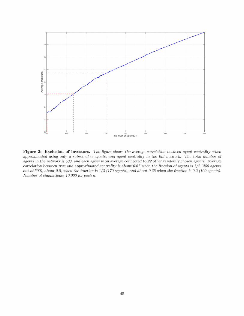
100 150 200 250 300 350 400 450 5000.2

0.3

0.4

0.5

0.6

0.7

0.8

0.9

1

Ave

rage

cor

elat

ion

Number of agents, n

Figure 3: Exclusion of investors. The figure shows the average correlation between agent centrality whenapproximated using only a subset of n agents, and agent centrality in the full network. The total number ofagents in the network is 500, and each agent is on average connected to 22 other randomly chosen agents. Averagecorrelation between true and approximated centrality is about 0.67 when the fraction of agents is 1/2 (250 agentsout of 500), about 0.5, when the fraction is 1/3 (170 agents), and about 0.35 when the fraction is 0.2 (100 agents).Number of simulations: 10,000 for each n.

45

0 20 40 60 80 100

0

10

20

30

40

50

60

70

80

90

100

Figure 4: Empirical Investor Network. The figure shows the empirical investor network, EIN, generated froma simulation of 50 trading periods, in a network with N = 100 traders, of which NI = 21 belong to the informationnetwork and NU = 79 are noise traders as in Figure 1. We assume that probabilities of q1 = 0.25, q2 = 0.5 and thethreshold for a connection is M = 1.

46

100

101

102

103

104

105

0

0.1

0.2

0.3

0.4

0.5

0.6

0.7

0.8

0.9

1

Degree − number of links

Cum

ulat

ive

dist

ribut

ion

Figure 5: Distribution of number of links. The figure shows the cumulative distribution function of the580,142 investors’ number of links (degrees) in the Empirical Investor Network (EIN), calculated by using actualtrades from Istanbul Stock Exchange over a 12 month period, January 1-December 31, 2005. Two agents are linkedwhen they trade in the same stock in the same direction within a 30 minute window at least M = 3 times. Themedian number of links is 159. Further, 90% of investors have less than 4,000 links. A small number of investorshave an extremely large number of links, leading to a significantly higher average number of links (1,781) than themedian.

47

−15 −14 −13 −12 −11 −10 −9 −8 −7 −6 −5 −4 −3 −2 −1 0 1 2 3 4 5 6 7 8 9 10 11 12 13 14 15

0.6

0.8

1

1.2

1.4

1.6

1.8

Day

Num

ber

of tr

ades

Figure 6: Trading activity. The figure shows the average hourly trading activity over time for the 11 events(described in the Internet Appendix), where Day 0 represents the point in time when each respective event wasreported in the news. A level higher than one represents a higher-than-average trading activity. The main increasein trading activity occurs between 11 and 3 trading days before the event is reported in the news.

48

Time window, ΔT 1 min 5 min 15 min 30 minNumber of links 161M 402M 731M 1.03BAverage number of links 277 693 1,260 1,781Median number of links 14 43 97 159Fraction of links 0.05% 0.12% 0.22% 0.31%Maximum number of links 116,720 171,823 219,123 251,943

Table 1: Summary statistics for EIN. The table shows summary statistics for the Empirical Investor Network(EIN) calculated by using actual trades from Istanbul Stock Exchange over a 12 month period, January 1-December31, 2005. Two agents are linked when they trade in the same stock in the same direction within 1, 5, 15 and 30minute window. Fraction of links is equal to average number of links divided by the number of potential links,which is equal to 580,142 during the time period. The threshold M = 3 is used.

49

A. All investors

CorrelationMean Std. dev. Median C D N Π Πe V

Centrality, C 4.99 12.1 0.64 1Degree, D 1,781 5,786 159 0.95 1Number of trades, N 149 1,467 8 0.71 0.60 1Profits, Π 0 2.0E5 -19.0 0.021 0.040 0.011 1Excess profits, Πe 0 1.3E5 -2.4 0.018 0.039 0.010 0.69 1Quantity, Q 9.1E5 20.4E6 11,340 0.27 0.43 0.14 0.21 0.18 1

B. All investors: log variables

CorrelationMean Std. dev. Median c d n μ μe v

Centrality, c -1.11 17.0 -0.43 1Degree, d 5.23 2.23 5.07 0.23 1Number of trades, n 2.41 2.00 2.08 0.17 0.93 1Returns, μ -0.014 0.085 -0.038 0.013 0.067 0.083 1Excess returns, μe -0.058 0.074 -0.0012 0.003 0.002 0.018 0.86 1Quantity, q 9.34 2.95 9.34 0.16 0.82 0.84 0.050 0.006 1

C. Split into individual and institutional investor groupsIndividual Institutional

Mean Std. dev. Median Mean Std. dev. Median

Centrality, C 4.95 12.0 0.64 44.6 41.6 36.1Degree, D 1,759 5,632 159 28,347 37,685 14,262Number of trades, N 144 1,350 8 6,805 18,390 1,460Profits, Π 23.7 2.0E5 -19.0 -28,070 1.0E6 2.98Excess profits, Πe -31.2 1.3E5 -2.4 37,040 3.6E5 8,680Quantity, Q 8.3E5 18.3E6 11,310 9.9E7 2.9E8 1.3E7

Table 2: Summary statistics for investors. The table shows summary statistics from the Empirical InvestorNetwork (EIN) calculated by using actual trades from Istanbul Stock Exchange over a 12 month period, January1-December 31, 2005. Two agents are linked when they trade in the same stock in the same direction within 30minute window at least M = 3 times during the period. Degree measures the number of links an agent is connectedto, including himself. Centrality is the eigenvector centrality. The variable μ is the value weighted return for alltrades of an investor for the entire year assuming a 30 day holding period for each trade and μe is the excess returnof the investor calculated similar to μ after adjusting return from each trade by the market return (ISE 100 indexreturn). Quantity is the sum of value of all transactions for an investor. The panel A and B shows summarystatistics for all investors and the correlation between the variables. The panel C splits investors into two groups,institutions and individual investors, and shows summary statistics.

50

A. One minute time window (ΔT = 1)Connection threshold 1 10 20 40 80

Number of links in first half, k1 129,146,847 11,174,905 5,014,735 2,150,618 903,097Number of links in second half, k2 136,493,437 12,006,001 5,539,690 2,442,503 1,057,607Number of overlaps, y 11,860,359 1,347,214 659,874 314,779 148,704

ECompletely random[y] 104,750 793 165 31 6

y/ECompletely random[y] 113.2 1,690 3,997 10,084 26,200

EDegree adjusted[y] 1,570,908

y/EDegree adjusted[y] 7.55

B. Five minute time window (ΔT = 5)Connection threshold 1 10 20 40 80

Number of links in first half, k1 259,906,612 33,510,862 16,238,861 7,420,656 326,895Number of links in second half, k2 274,034,135 35,975,750 17,924,953 8,449,474 3,817,082Number of overlaps, y 30,556,857 4,659,221 2,400,323 1,180,224 559,647

ECompletely random[y] 423,237 7,164 1730 373 74

y/ECompletely random[y] 72.2 650 1,388 3,168 7,548

EDegree adjusted[y] 5,017,607

y/EDegree adjusted[y] 6.09

Table 3: Stability of EIN. The table shows the stability of the empirical investor network across the first andsecond half year in the sample period of January 1-December 31, 2005. Two agents are linked when they tradein the same stock in the same direction multiple times, determined by the connection threshold, within the timewindow. In Panel A the time window is 1 minute and in Panel B the time window is 5 minutes. The connectionthreshold, M , is between 1 and 80 and displayed in columns. The total number of potential connections betweeninvestors is K = N(N − 1)/2 = 1.68× 1011 (counting the relationship that investors i and j are linked as one link,i.e., not double counting bidirectional links), where N = 580, 142 is the number of investors. Number of overlaps, ymeasures the number of intersecting links between the first and second half of the year. ECompletely random[y] is

the expected number of intersecting link between the first and second half of the year if the networks are random.EDegree adjusted[y] is also a measure of expected number of intersecting links between the first and second periods

and corrects for the degree distributions observed in practice.

51

A.Retu

rns

12

34

56

78

910

11

OLS

OLS

OLS

OLS

OLS

OLS

OLS

t−

error

t−

error

Ramsey

Ramsey

Cen

trality

(c)

0.0027

0.0060

0.0032

0.0060

>20

14.1

3.7

13.8

Degree(d)

0.0027

-0.0091

-0.0062

-0.0091

>20

−18.6

-6.4

-18.4

RescaledCen

trality

(c−

d)

0.00003

0.0038

0.0008

0.0038

4.13

9.2

0.94

8.9

#oftrades

(n)

0.0037

0.0092

0.0063

0.0072

0.0041

0.0092

0.0062

>20

>20

>20

19.9

19.0

>20

>20

Quantity

(q)

0.0014

-0.0017

-0.0019

-0.0013

-0.0015

-0.0017

-0.0015

>20

<−2

0<

−20

−8.8

-10.3

<−2

0<

−20

R2

0.0043

0.0041

3.1E-5

0.0040

0.0024

0.0091

0.0083

Δμ

0.6%

0.6%

0.05%

0.7%

0.4%

1.2%

0.1%

0.7%

0.001%

1.2%

0.1%

B.Excess

retu

rns

12

34

56

78

910

11

OLS

OLS

OLS

OLS

OLS

OLS

OLS

t−

error

t−

error

Ramsey

Ramsey

Cen

trality

(c)

0.0001

0.0090

0.0066

0.0090

1.52

>20

8.8

>20

Degree(d)

-0.0003

-0.0136

-0.0114

-0.0137

-0.43

<−2

0−1

3.4

<−2

0RescaledCen

trality

(c−

d)

0.00001

0.0056

0.0031

0.0056

1.7

15.6

4.3

15.4

#oftrades

(n)

0.00069

0.0063

0.0019

0.0056

0.0009

0.0063

0.0018

13.3

>20

19.7

17.8

4.7

>20

18.8

Quantity

(q)

0.00014

-0.0004

-0.0008

-0.0004

-0.0008

-0.0004

-0.0008

4.2

-6.4

-12.2

-3.4

-6.0

-6.7

-12.6

R2

0.000041

3.5E-9

5.2E-6

0.00031

0.000029

0.0033

0.0010

Δμ

0.01%

-0.004%

0.02%

0.1%

0.04%

1.8%

0.2%

1.3%

0.1%

1.8%

0.2%

Table

4:

Centrality

and

Retu

rns.

Thetable

displaysresultsfrom

regressionsofvalueweightedreturns(P

anel

A)andvalueweightedexcess

returns(P

anel

B)onlogcentrality,logdegree,

logrescaledcentrality,lognumber

oftrades

andlogquantity.Each

columnrepresents

aregression.

Thefirstrow

displayscoeffi

cients

whilethesecondrow

displaysthet-statistics.

Thefirst7columnsdisplayresultsfrom

OLSregressions,

columns

8-9

displayresultsfrom

aregressionthatis

robust

toheavy-tailed

errorterm

s,andcolumns10-11displayresultsfrom

iterativelyre-w

eightedleast

square

regression(usingRamsey’sE-function).

Thevariable

μisthevalueweightedreturn

foralltrades

ofaninvestorfortheentire

yearassuminga

30day

holdingperiodforeach

tradeandμeis

theexcess

return

oftheinvestorcalculatedsimilarto

μafter

adjustingreturn

from

each

tradebythe

market

return

(ISE

100index

return).

Degreemeasuresthenumber

oflinksanagentis

connectedto,includinghim

self.Centrality

istheeigenvector

centrality.Tradingquantity

isthesum

ofvalueofalltransactionsforeach

investor.

And#

oftrades

isthetotalnumber

oftrades

foreach

investor.

Thevariables,

Δμ

andΔμehighlighttheeconomic

significance

oftheresultsbyshow

ingthechangein

returns(andexcess

returns),given

aone

standard

deviationincrease

ofthevariable

inunivariate

regressionsandcentrality

orrescaledcentrality

inmultivariate

regressions,allelse

equal.The

Δt=30-m

inuteswindow

isused.Thedata

istruncated,such

thatinvestors

inthebottom

twopercentilesandtoptw

opercentilesofconnectedness

are

discarded

from

thedata.

52

A.Retu

rns

Threshold

(M)

12

34

56

78

910

Med

ian#

links

673

294

159

119

86

73

58

52

44

39

Cen

trality

(c)

0.012

0.098

0.0060

0.0035

0.0019

0.0014

0.00001

0.00015

0.00019

0.00019

>20

19.8

14.1

9.3

5.8

6.3

0.19

6.1

13.0

16.3

Degree(d)

-0.014

-0.013

-0.0091

-0.0061

-0.0042

-0.0033

-0.0019

-0.0017

-0.0018

-0.0017

<−2

0<

−20

-18.6

-13.6

-10.5

-10.7

-7.5

-11.1

-11.2

-10.9

#oftrades

(n)

0.0084

0.095

0.0092

0.0087

0.0085

0.0079

0.0078

0.0076

0.0076

0.0075

>20

>20

>20

>20

>20

>20

>20

>20

>20

>20

Quantity

(q)

-0.0017

-0.0016

-0.0017

-0.0017

-0.0017

-0.0017

-0.0018

-0.0018

-0.0018

-0.0017

<−2

0<

−20

<−2

0<

−20

<−2

0<

−20

<−2

0<

−20

<−2

0<

−20

R2

0.01

0.010

0.0091

0.0088

0.0086

0.0085

0.0082

0.0084

0.0087

0.0087

Δμ

2.2%

1.9%

1.2%

0.7%

0.4%

0.3%

0.01%

0.1%

0.2%

0.2%

B.Excess

retu

rns

Threshold

(M)

12

34

56

78

910

Med

ian#

links

673

294

159

119

86

73

58

52

44

39

Cen

trality

(c)

0.0098

0.013

0.0090

0.0059

0.0043

0.0015

0.0005

0.0001

0.0001

0.0001

>20

>20

>20

17.9

15.4

7.9

3.7

3.1

5.9

6.9

Degree(d)

0.013

-0.017

-0.014

-1.02

-0.0081

-0.0049

-0.0032

-0.0026

-0.0024

-0.0023

<−2

0<

−20

<−2

0<

−20

<−2

0-18.4

-15.1

-19.3

-18.0

-17.0

#oftrades

(n)

0.0038

0.0059

0.0063

0.0059

0.0055

0.0048

0.0042

0.0040

0.0037

>20

>20

>20

>20

>20

>20

>20

>20

>20

>20

Quantity

(q)

-0.0004

-0.0003

-0.0004

-0.0004

-0.0005

-0.0004

-0.0006

-0.0005

-0.0006

-0.0006

-6.6

−4.8

−6.38

-6.54

-8.1

-7.1

-8.8

-8.9

-9.1

-8.4

R2

0.0032

0.0044

0.0033

0.0025

0.0020

0.0016

0.0013

0.0012

0.0012

0.0010

Δμ

1.8%

2.6%

1.8%

1.2%

0.9%

0.3%

0.1%

0.03%

0.1%

0.1%

Table

5:Differentth

resh

olds.

Thetable

displaysresultsfrom

OLSregressionsofvalueweightedreturns(P

anel

A)andvalueweightedexcess

returns(P

anel



oftrades

andlogquantity,similarto

Table

4,when

varyingthe

threshold

forconnections,M

,between1and10.Each

columnrepresents

aregression.Thefirstrowdisplayscoeffi

cients

whilethesecondrow

displays

thet-statistics.

Thevariable

μis

thevalueweightedreturn

foralltrades

ofaninvestorfortheentire

yearassuminga30day


tradeandμeis

theexcess

return


μafter

adjustingreturn

from

each

tradebythemarket

return

(ISE

100index

return).


oflinksanagentis

connectedto,includinghim

self.Centrality

istheeigenvectorcentrality.Tradingquantity

isthesum


investor,

and#

oftrades

isthetotalnumber

oftrades

foreach

investor.

Thevariables,

ΔμandΔμe

highlighttheeconomic

significance

oftheresultsbyshow

ingthechangein

returns(andexcess

returns),given

aonestandard

deviationincrease

ofthe

centrality,allelse

equal.

TheΔt=30-m

inuteswindow

isused.Thedata

istruncated,such

thatinvestors

inthebottom


opercentilesofconnectednessare

discarded

from

thedata.

53

A. Original set of 11 events1 2 3 4 5

Centrality Centrality Degree Number of trades Trading Quantityc c d n q

βOLS -0.15 -1.0 1.0 -0.19 -0.03

tOLS < −20 -15.0 14.9 -11.2 -3.3tt−error -15.1 -6.4 5.2 -1.9 -2.0tRamsey < −20 -14.8 14.7 -10.8 -3.2

B. Extended set of 27 events

Centrality Centrality Degree Number of trades Trading Quantityc c d n q

βOLS -0.19 -1.1 1.3 -0.31 -0.18

tOLS -19.4 -10.2 12.7 -11.6 -15.7tt−error -13.7 -6.4 7.0 -4.3 -9.2tRamsey -19.4 -10.2 12.7 -11.6 -15.6

Table 6: Trading time versus centrality. The table shows the trading time (T ) regressed on log-centrality(c) in univariate regressions (first column), and in multivariate regressions (columns 2-5), together with log-degree(d) log-number of trades (n) and log-trading-quantity (q). For a detailed definition of these variables, see Table 4.Panel A includes 11 events, and Panel B includes an extended set of 27 events. In both panels, the first two rowsshows the coefficient and t-statistics from OLS regressions. Rows 3 and 4 display t-statistics from a regressionthat is robust to heavy-tailed error terms and from iteratively re-weighted least square regression (using Ramsey’sE-function), respectively.

54

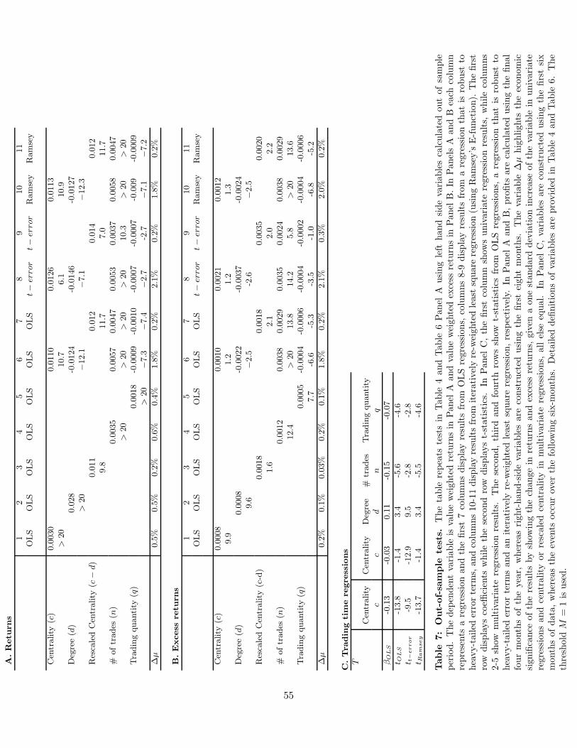
A.Retu

rns

12

34

56

78

910

11

OLS

OLS

OLS

OLS

OLS

OLS

OLS

t−

error

t−

error

Ramsey

Ramsey

Cen

trality

(c)

0.0030

0.0110

0.0126

0.0113

>20

10.7

6.1

10.9

Degree(d)

0.028

-0.0124

-0.0146

-0.0127

>20

−12.1

−7.1

−12.3

RescaledCen

trality

(c−

d)

0.011

0.012

0.014

0.012

9.8

11.7

7.0

11.7

#oftrades

(n)

0.0035

0.0057

0.0047

0.0053

0.0037

0.0058

0.0047

>20

>20

>20

>20

10.3

>20

>20

Tradingquantity

(q)

0.0018

-0.0009

-0.0010

-0.0007

-0.0007

-0.009

-0.0009

>20

−7.3

−7.4

−2.7

-2.7

−7.1

−7.2

Δμ

0.5%

0.5%

0.2%

0.6%

0.4%

1.8%

0.2%

2.1%

0.2%

1.8%

0.2%

B.Excess

retu

rns

12

34

56

78

910

11

OLS

OLS

OLS

OLS

OLS

OLS

OLS

t−

error

t−

error

Ramsey

Ramsey

Cen

trality

(c)

0.0008

0.0010

0.0021

0.0012

9.9

1.2

1.2

1.3

Degree(d)

0.0008

-0.0022

-0.0037

-0.0024

9.6

−2.5

-2.6

−2.5

RescaledCen

trality

(c-d)

0.0018

0.0018

0.0035

0.0020

1.6

2.1

2.0

2.2

#oftrades

(n)

0.0012

0.0038

0.0029

0.0035

0.0024

0.0038

0.0029

12.4

>20

13.8

14.2

5.8

>20

13.6

Tradingquantity

(q)

0.0005

-0.0004

-0.0006

-0.0004

-0.0002

-0.0004

-0.0006

7.7

-6.6

-5.3

-3.5

-1.0

-6.8

-5.2

Δμ

0.2%

0.1%

0.03%

0.2%

0.1%

1.8%

0.2%

2.1%

0.3%

2.0%

0.2%

C.Tra

dingtimere

gre

ssions

TCen

trality

Cen

trality

Degree

#trades

Tradingquantity

cc

dn

q

βOLS

-0.13

-0.03

0.11

-0.15

-0.07

t OLS

-13.8

-1.4

3.4

-5.6

-4.6

t t−error

-9.5

-12.9

9.5

-2.8

-2.8

t Ram

sey

-13.7

-1.4

3.4

-5.5

-4.6

Table

7:

Out-of-sa

mple

tests.

Thetable

repeats

testsin

Table

4andTable

6Panel

Ausingleft

handsidevariablescalculatedoutofsample

period.Thedep

endentvariable

isvalueweightedreturnsin

Panel

Aandvalueweightedexcess

returnsin

Panel

B.In

PanelsA

andB

each

column

represents

aregressionandthefirst7columnsdisplayresultsfrom

OLSregressions,

columns8-9

displayresultsfrom

aregressionthatis

robust

toheavy-tailed

errorterm


iterativelyre-w

eightedleast

square

regression(usingRamsey’sE-function).

Thefirst

row

displayscoeffi

cients

whilethesecondrow

displayst-statistics.

InPanel

C,thefirstcolumnshow

sunivariate

regressionresults,

whilecolumns

2-5

show

multivariate

regressionresults.

Thesecond,thirdandfourthrowsshow

t-statisticsfrom

OLSregressions,

aregressionthatis

robust

toheavy-tailed

errorterm

sandaniterativelyre-w

eightedleast

square

regression,respectively.

InPanel

AandB,profits

are

calculatedusingthefinal

fourmonthsoftheyear,

whereasright-hand-sidevariablesare

constructed

usingthefirsteightmonths.

Thevariable

Δμ

highlights

theeconomic

significance

oftheresultsbyshow

ingthechangein

returnsandexcess

returns,

given

aonestandard

deviationincrease

ofthevariable

inunivariate



inmultivariate

regressions,

allelse

equal.

InPanel

C,variablesare

constructed

usingthefirstsix

monthsofdata,whereastheevents

occurover

thefollow

ingsix-m

onths.

Detailed

definitionsofvariablesare

provided

inTable

4andTable

6.The

threshold

M=

1is

used.

55

A.Retu

rns

High-inform

ation

periods

Low-inform

ation

periods

OLS

t−

error

Ramsey

OLS

t−

error

Ramsey

Cen

trality

(c)

0.019

0.015

0.019

0.0008

0.0025

0.0014

>20

12.5

>20

1.7

2.6

2.9

Degree(d)

-0.016

-0.013

-0.017

0.0015

-0.0018

0.0007

<−2

0-10.7

<−2

03.0

-1.9

1.3

#oftrades

(n)

0.0064

0.0059

0.0064

0.0007

0.0006

0.0007

>20

>20

>20

6.8

3.0

7.2

Quantity

(q)

-0.0054

-0.0049

-0.0054

-0.0010

-0.0007

-0.0010

<−2

0<

−20

<−2

0-14.5

-5.0

-14.4

R2

0.016

0.0031

Δμ

3.6%

2.8%

3.6%

0.2%

0.5%

0.3%

B.Excess

retu

rns

High-inform

ation

periods

Low-inform

ation

periods

OLS

t−

error

Ramsey

OLS

t−

error

Ramsey

Cen

trality

(c)

0.010

0.0080

0.010

0.0025

0.0026

0.0029

19.6

7.9

19.8

5.9

3.0

6.8

Degree(d)

-0.010

-0.0088

-0.011

-0.0023

-0.0033

-0.0028

<−2

0-8.6

<−2

0-5.2

-3.8

-6.5

#oftrades

(n)

0.0023

0.0017

0.0022

-0.0001

0.000003

-0.0004

19.3

7.0

17.8

-0.7

-2.3

0.05

Quantity

(q)

-0.0019

-0.0013

-0.0018

-0.0001

0.00003

-0.0002

<−2

0-7.9

<−2

0-2.4

-2.3

-2.8

R2

0.0032

0.00004

Δμ

1.9%

1.5%

1.9%

0.5%

0.5%

0.6%

Table

8:High-andlow-inform

ationperiods.

Thetable

displaysresultsfrom


anel

A)andvalueweighted

excess

returns(P

anel

B),when

totaltimeperiodissplitinto

high-inform

ationmonths,in

whichthereweremanyearningsannouncements

(March178,

May

182,August

176,andNov

170),

andlow-inform

ationmonths,

inwhichtherewerefew

such

announcements

(January

8,February

41,April109,

June87,July

10,October

55,andDecem

ber

80).

Thefirstrow

displayscoeffi

cients

whilethesecondrow

displaysthet-statistics.

Columnscolumns

2-4

displayresultsin

high-inform

ationmonths(O

LS,heavy-tailed

errorterm

s,anditerativelyre-w

eightedleast

square

withRamsey’s

E-function).

Columns5-7

displaytheregressionsin

thelow-inform

ationmonths.

Thevariable

μis


foralltrades

ofaninvestorforthe

entire

yearassuminga30day


tradeandμeistheexcess

return


μafter

adjustingreturn

from

each

tradebythemarket

return

(ISE

100index

return).


oflinksanagentisconnectedto,includinghim

self.Centrality


isthesum


investor.

And#

oftrades

isthetotalnumber

oftrades

foreach

investor.

Thevariables,ΔμandΔμehighlighttheeconomic

significance

oftheresultsbyshow

ingthechangein

returns(andexcess

returns),

given

aonestandard

deviationincrease

ofthevariable

inunivariate



inmultivariate

regressions,

all

else

equal.

TheΔt=30-m

inuteswindow

isused.Thedata

istruncated,such

thatinvestors

inthebottom


opercentilesof

connectednessare

discarded

from

thedata.

56

A.Retu

rns

12

34

56

78

910

11

OLS

OLS

OLS

OLS

OLS

OLS

OLS

t−

error

t−

error

Ramsey

Ramsey

Cen

trality

(c)

-0.012

0.0007

0.013

0.011

<−2

00.48

4.1

6.7

Degree(d)

-0.012

0.0012

-0.0010

-0.0091

<−2

00.73

-3.2

-5.4

RescaledCen

trality

(c−

d)

0.058

0.0040

0.015

0.013

>20

2.6

4.8

8.4

#oftrades

(n)

-0.013

-0.013

-0.014

-0.013

-0.011

-0.013

-0.014

<−2

0<

−20

<−2

0−1

4.8

<−2

0<

−20

<−2

0Quantity

(q)

-0.0081

-0.0013

0.0016

0.0016

0.0048

0.0016

0.0039

<−2

0−6

.78.1

7.8

5.4

7.6

19.3

R2

0.016

0.022

0.0059

0.022

0.017

0.023

0.023

Δμ

1.9%

2.0%

1.1%

2.2%

2.0%

0.1%

0.08%

2.0%

0.3%

1.7%

0.3%

B.Excess

retu

rns

12

34

56

78

910

11

OLS

OLS

OLS

OLS

OLS

OLS

OLS

t−

error

t−

error

Ramsey

Ramsey

Cen

trality

(c)

0.0041

0.016

0.0096

0.018

>20

13.2

4.0

14.8

Degree(d)

0.0038

-0.015

-0.00934

-0.017

>20

−11.7

−3.7

-13.7

RescaledCen

trality

(c−

d)

0.0059

0.016

0.0096

0.018

6.0

13.6

4.0

15.0

#oftrades

(n)

0.0038

0.0048

0.0057

0.0025

0.0026

0.0045

0.0050

>20

16.2

>20

4.1

6.2

14.8

>20

Quantity

(q)

0.0019

-0.0004

-0.0008

0.0015

-0.0008

0.0004

0.0005

>20

-6.2

-5.6

4.9

-6.0

2.7

3.1

R2

0.0031

0.0029

0.0001

0.0033

0.0016

0.0040

0.0040

Δμ

0.7%

0.6%

0.2%

0.7%

0.5%

2.5%

0.3%

1.5%

0.2%

2.9%

0.4%

Table

9:Realizedretu

rns.

Thetable

displaysresultsfrom


anelA)andvalueweightedexcess

returns(P

anel



oftrades

andlogvolume.

Each

columnrepresents

aregression.Thefirstrow

displayscoeffi

cients

whilethesecondrowdisplaysthet-statistics.


OLSregressions,columns8-9

displayresults

from

aregressionthatis

robust

toheavy-tailed

errorterm


iterativelyre-w

eightedleast

square

regression

(usingRamsey’s

E-function).

Thevariable

μis


foralltrades

ofaninvestorandμeis

theexcess

return

oftheinvestor.

Incontrast

toTable

4,realizedreturnsofclosedpositionsare

usedin

thereturn

calculations.


oflinksanagentisconnected

to,includinghim

self.Centrality


isthesum


investor.

And#

oftrades

isthetotalnumber

oftrades

foreach

investor.

Thevariables,ΔμandΔμehighlighttheeconomic

significance

oftheresultsbyshow

ingthechangein

returns(andexcess

returns),given

aonestandard

deviationincrease

ofthevariable

inunivariate



inmultivariate

regressions,allelse

equal.TheΔt=30-m

inuteswindow

isused.Thedata

istruncated,such

thatinvestors

inthebottom

twopercentiles

andtoptw

opercentilesofconnectednessare

discarded

from

thedata.

57

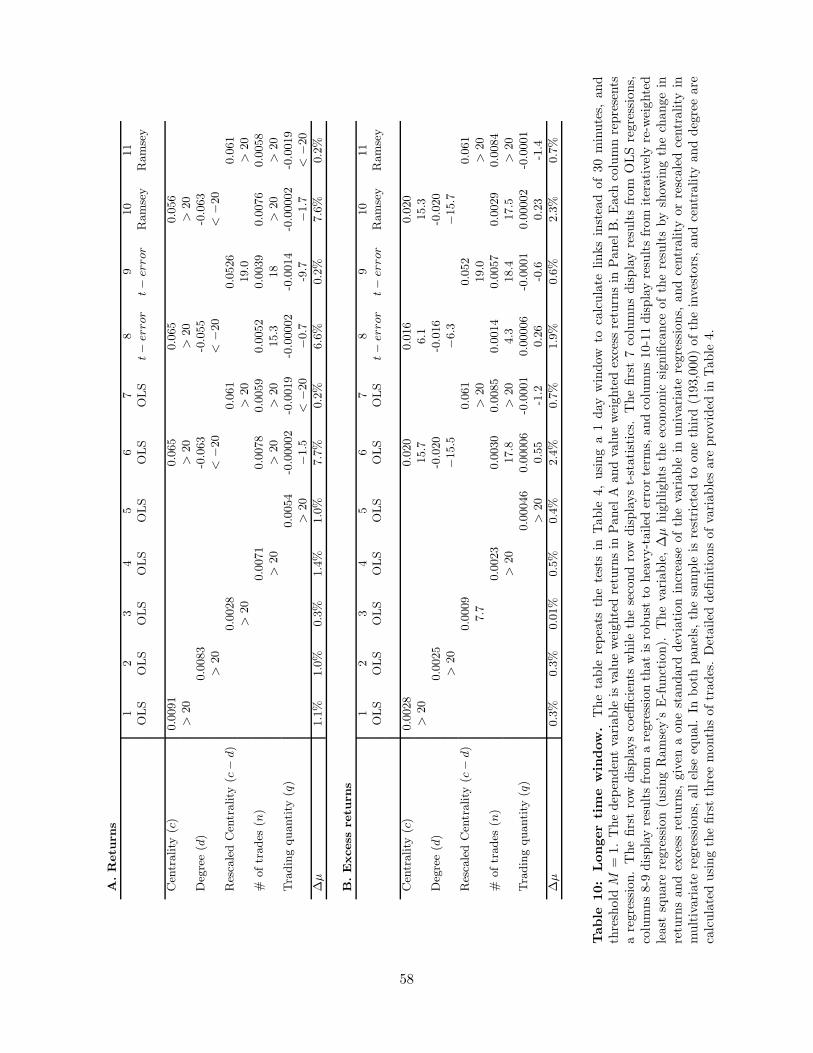
A.Retu

rns

12

34

56

78

910

11

OLS

OLS

OLS

OLS

OLS

OLS

OLS

t−

error

t−

error

Ramsey

Ramsey

Cen

trality

(c)

0.0091

0.065

0.065

0.056

>20

>20

>20

>20

Degree(d)

0.0083

-0.063

-0.055

-0.063

>20

<−2

0<

−20

<−2

0RescaledCen

trality

(c−

d)

0.0028

0.061

0.0526

0.061

>20

>20

19.0

>20

#oftrades

(n)

0.0071

0.0078

0.0059

0.0052

0.0039

0.0076

0.0058

>20

>20

>20

15.3

18

>20

>20

Tradingquantity

(q)

0.0054

-0.00002

-0.0019

-0.00002

-0.0014

-0.00002

-0.0019

>20

−1.5

<−2

0−0

.7-9.7

−1.7

<−2

0

Δμ

1.1%

1.0%

0.3%

1.4%

1.0%

7.7%

0.2%

6.6%

0.2%

7.6%

0.2%

B.Excess

retu

rns

12

34

56

78

910

11

OLS

OLS

OLS

OLS

OLS

OLS

OLS

t−

error

t−

error

Ramsey

Ramsey

Cen

trality

(c)

0.0028

0.020

0.016

0.020

>20

15.7

6.1

15.3

Degree(d)

0.0025

-0.020

-0.016

-0.020

>20

−15.5

−6.3

−15.7

RescaledCen

trality

(c−

d)

0.0009

0.061

0.052

0.061

7.7

>20

19.0

>20

#oftrades

(n)

0.0023

0.0030

0.0085

0.0014

0.0057

0.0029

0.0084

>20

17.8

>20

4.3

18.4

17.5

>20

Tradingquantity

(q)

0.00046

0.00006

-0.0001

0.00006

-0.0001

0.00002

-0.0001

>20

0.55

-1.2

0.26

-0.6

0.23

-1.4

Δμ

0.3%

0.3%

0.01%

0.5%

0.4%

2.4%

0.7%

1.9%

0.6%

2.3%

0.7%

Table

10:

Longertime

window.

Thetable

repeats

thetestsin

Table

4,usinga1day

window

tocalculate

linksinsteadof30minutes,

and

threshold

M=

1.Thedep

endentvariable

isvalueweightedreturnsin

Panel

Aandvalueweightedexcess

returnsin

Panel

B.Each

columnrepresents

aregression.Thefirstrow

displayscoeffi

cients

whilethesecondrow

displayst-statistics.


OLSregressions,

columns8-9

displayresultsfrom

aregressionthatisrobust

toheavy-tailed

errorterm


iterativelyre-w

eighted

least

square

regression(usingRamsey’s

E-function).

Thevariable,Δμhighlights

theeconomic

significance

oftheresultsbyshow

ingthechangein

returnsandexcess

returns,

given

aonestandard

deviationincrease

ofthevariable

inunivariate

regressions,

andcentrality


inmultivariate

regressions,

allelse

equal.

Inboth

panels,

thesample

isrestricted

toonethird(193,000)oftheinvestors,andcentrality

anddegreeare

calculatedusingthefirstthreemonthsoftrades.Detailed

definitionsofvariablesare

provided

inTable

4.

58

investor networks in the stock market -...

Documents