investments
DESCRIPTION
Investments solution manual by Charles P. JonesTRANSCRIPT
PART ONE: BACKGROUND
Chapter 1: Understanding Investments
CHAPTER OVERVIEW
Chapter 1 is designed to be a standard introductory chapter. As such, its purpose is to introduce students to the subject of Investments, explain what this topic is concerned with from a summary viewpoint, and outline what the remainder of the text will cover. It defines important terms such as investments, security analysis, portfolio management, expected and realized rate of return, risk-free rate of return, and risk.
IT IS IMPORTANT TO NOTE THAT Chapter 1 discusses some important issues, such as the expected return--risk tradeoff that governs the investment process, the uncertainty that dominates investment decisions, the globalization of investments, the impact of institutional investors, and the basic idea behind the Efficient Market Hypothesis. As such, the chapter is important in setting the tone for the entire text and in explaining to the reader what Investments is all about. It establishes a basic framework for the course without going into too much detail at the outset.
Chapter 1 also contains some material that will be of direct interest to students, including the importance of studying investments (using illustrations of the wealth that can be accumulated by compounding over long periods of time) and investments as a profession. The CFA designation is discussed, and the Appendix contains a more detailed description of the CFA program.
1
Equally important, Chapter 1 does not cover calculations and statistical concepts, data on asset returns, and so forth, either in the chapter or an appendix. The author feels strongly that Chapter 1 is not the place to do this when students in most cases have no real idea what the subject is all about. They are not ready for this type of important material, and since it will not be used immediately they will lose sight of why it was introduced. The author believes that it is much more effective to introduce the students thoroughly to what the subject involves without getting into technical details at the very beginning of the course.
It is highly desirable for instructors to add their own viewpoints at the outset of the course, perhaps using recent stories from the popular press to emphasize what investments is concerned with, why students should be interested in the subject, and so forth.
CHAPTER OBJECTIVES
To introduce students to the subject matter of Investments from an overall viewpoint, including terminology.
To explain the basic nature of the investing decision as a tradeoff between expected return and risk.
To explain that the decision process consists of security analysis and portfolio management and that external factors affect this decision process. These factors include uncertainty, the necessity to think of investments in a global context, the environment involving institutional investors, and the impact of the internet on investing.
To organize the remainder of the text.
2

MAJOR CHAPTER HEADINGS [Contents]
The Nature of Investments
Some Definitions[investment; investments; financial and real assets; marketable securities; portfolio]
A Perspective on Investing in Financial Assets[investing is only one part of overall financial decisions]
Why Do We Invest?[to increase monetary wealth]
The Importance of Studying Investments
The Personal Aspects[most people make some type of investment decisions; examples of wealth accumulation as a result of compounding; how an understanding of the subject will help students when reading the popular press]
Investments as a Profession[various jobs, salary ranges; Chartered Financial Analyst designation]
Understanding the Investment Decision Process
The Basis of Investment Decisions[expected return; realized return; risk; risk-averse investor; the Expected-Return--Risk Tradeoff; diagram of tradeoff; ex post vs. ex ante; risk-free rate of return, RF]
Structuring the Decision Process[a two-step process: security analysis and portfolio management; passive and active investment strategies; the Efficient Market Hypothesis]
3
Important Considerations in the Investment Decision Process for Today’s Investors
The Great Unknown[uncertainty dominates decisions--the future is unknown!]
The Global Investments Arena[the importance of foreign markets; the Euro; emerging markets]
The New Economy vs. The Old Economy[old economy stocks are the traditional service, consumer and financial companies; new economy stocks have a focus on technology, e-commerce, etc. In most cases the latter have little or no earnings, and certainly don’t pay dividends in virtually all cases]
The Rise of the Internet[using the internet to invest; the impact of the sharp market decline in 2000-2001]
Institutional Investors [individual investors compete with institutional investors, but individuals are the beneficiaries of institutional investor activity, such as pension funds; the issue of market efficiency]
Organizing the Text
[Background; Realized and Expected Returns and Risk; Bonds; Stocks; Security Analysis, including both fundamental and technical analysis; Derivative Securities; Portfolio Theory and Capital Market Theory; the Portfolio Management Process and Measuring Portfolio Performance]
Appendix 1-A The Chartered Financial Analyst Program
[a description of the CFA program]
POINTS TO NOTE ABOUT CHAPTER 1
4
Tables and Figures
There is only one figure in Chapter 1, but it is crucial because it the basis of investing decisions--indeed, it is the basis of all finance decisions. It shows the expected return--risk tradeoff available to investors. This diagram may be desirable to use as a transparency because it can be used to generate much useful discussion, including:
The upward-sloping tradeoff that dominates Investments. The role of RF, the risk-free rate of return. The importance of risk in all discussions of investing. The different types of financial assets available. The distinction between realized and expected return.
NOTE: THIS DIAGRAM IS RELEVANT ON THE FIRST DAY OF CLASS, AND THE LAST. IT IS A GOOD WAY TO START THE COURSE, AND TO END IT.
Table 1-1 shows wealth accumulations possible from an IRA-type investment. It typically generates considerable student interest to see the ending wealth that can be produced by compounding over time. This type of example can be related to 401 (k) plans, which are quickly becoming of primary importance to many people.
Boxed Inserts
Box 1-2 is a good example of why Investments is a difficult subject. It highlights some predictions by the investing community, which did not work too well. This Box Insert is taken from a regular feature of Smart Money, and offers a good opportunity to start informing students about the popular press magazines and newspapers available to investors.
Box 1-2 is a discussion of spinoffs. The discussion indicates that spinoffs do well over a period of one to three years, unlike many IPOs. Most importantly, individual investor can invest in spinoffs as well as, or better than, institutional investors. In other words, this is an opportunity for individual investors to compete effectively in the investing arena. Professional managers often dump spinoffs because they do not fit in with what they are currently doing. Analysts often ignore them. Thus, this can be an opportunity for individual investors.
5
ANSWERS TO END-OF-CHAPTER QUESTIONS
1-1. Investments is the study of the investment process. An investment is defined as the commitment of funds to one or more assets to be held over some future time period.
1-2. Traditionally, the investment decision process has been divided into security analysis and portfolio management.
• Security analysis involves the analysis and valuation of individual securities; that is, estimating value, a difficult job at best.
• Portfolio management utilizes the results of security analysis to construct portfolios. As explained in Part II, this is important because a portfolio taken as a whole is not equal to the sum of its parts.
1-3. The study of investments is important to many individuals because almost everyone has wealth of some kind and will be faced with investment decisions sometime in their lives. One important area where many individuals can make important investing decisions is that of retirement plans, particularly 401 (k) plans. In addition, individuals often have some say in their retirement programs, such as allocation decisions to cash equivalents, bonds, and stocks.
The dramatic stock market gains of 1995,1996, 1997, and 1998 illustrate almost better than anything else the importance of studying investments. Investors who were persuaded in the past to go heavily, or all, in stocks have reaped tremendous gains in their retirement assets as well as in their taxable accounts.
1-4. A financial asset is a piece of paper evidencing some type of financial claim on an issuer, whether private (corporations) or public (governments).
A real asset, on the other hand, is a tangible asset such as gold coins, diamonds, or land.
1-5. Investments, in the final analysis, is simply a risk-return tradeoff. In order to have a chance to earn a
13
return above that of a risk-free asset, investors must take risk. The larger the return expected, the greater the risk that must be taken.
The risk-return tradeoff faced by investors making investment decisions has the following characteristics:
The risk-return tradeoff is upward sloping because investment decisions involve expected returns (vertical axis) versus risk (horizontal axis).
The vertical intercept of this tradeoff is RF, the risk free rate of return available to all investors.
1-6. An investor would expect to earn the risk-free rate of return (RF) when he or she invests in a risk-free asset and is, therefore, at the zero risk point on the horizontal axis in Figure 1-1.
1-7. False. Risk-averse investors assume risk if they expect to be adequately compensated for it.
1-8. The basic nature of the investment decision for all investors is the upward-sloping tradeoff between expected return and risk that must be dealt with each time an investment decision is made.
1-9. Expected return is the anticipated return for some future time period, whereas realized return is the actual return over some past period.
1-10. In general, the term risk as used in investments refers to adverse circumstances affecting the investor’s position. Risk can be defined in several different ways. Risk is defined here as the chance that the actual return on an investment will differ from its expected return.
Beginning students will probably think of default risk and purchasing power risk very quickly. Some may be aware of interest rate risk and market risk without fully understanding these concepts (which will be explained in later chapters). Other risks include political risk and liquidity risk. Students may also remember financial risk and business risk from their managerial finance course.
14
1-11. Although risk is the most important constraint, investors face other constraints. These include:
legal constraints taxes transaction costs income requirements exchange listing (or lack thereof) diversification requirements
1-12. All rational investors are risk averse because it is not rational when investing to assume risk unless one expects to be compensated for doing so. All investors do not have the same degree of risk aversion. They are risk averse to varying degrees, requiring different risk premiums in order to invest.
1-13. The external factors affecting the decision process are:
(1) uncertainty(2) the investing environment (institutional investors
vs individual investors)(3) the globalization of the investing process(4) the rise of the internet
The most important factor is uncertainty, the paramount factor with which all investors must deal. Uncertainty dominates investments, and always will.
1-14. Institutional investors include bank trust departments, pension funds, mutual funds (investment companies), insurance companies, and so forth. Basically, these financial institutions own and manage portfolios of securities on behalf of various clienteles.
They affect the investments environment (and therefore individual investors) through their actions in the marketplace, buying and selling securities in large dollar amounts. However, although they appear to have several advantages over individuals (research departments, expertise, etc.), reasonably informed individuals should be able to perform as well as institutions, on average, over time. This relates to the issue of market efficiency.
15
1-15. An efficient market is one in which the prices of securities quickly and (on balance) correctly reflect information about securities. In such a market, the
prices of securities do not depart for long from their justified economic values.
1-16. An efficient market is significant to investors because it will affect their behavior. Quite a few actions, such as performing the same security analysis as everyone else, are of no value in an efficient market. Technical analysis is ruled out, as is standard fundamental analysis. Portfolio management is also affected, with fewer actions justified than would be the case if the market is not efficient.
1-17. Required rates of return differ as the risk of an investment varies. Treasury bonds are less risky than corporates, and therefore have a lower required rate of return.
1-18. Investors should be concerned with international investing for several important reasons. First, more opportunities are now available to investors in the form of mutual funds and closed-end funds investing in foreign stocks and bonds. Second, the returns may be better in foreign markets at a particular point in time than in the U. S. markets. Third, by investing in foreign securities, investors may be able to reduce the risk of their portfolios. Fourth, many U. S. companies are increasingly affected by conditions abroad--for example, Coca Cola derives most of its revenue and profits from foreign operations. U. S. companies clearly are significantly affected by foreign competitors.
The exchange rate (currency risk) is an important part of all decisions to invest internationally. As discussed later in the text, currency risk affects investment returns, both positively and negatively.
The creation of the Euro presents new opportunities and challenges for investors. This is a significant change for European financial markets, and it is too early to tell what will happen as a result of these changes.
16
1-19. The “Old Economy” refers to the traditional manufacturing, service, and financial companies, many of which are very large corporations such as IBM, Exxon, and Merrill Lynch. These companies typically show positive earnings, and many pay dividends. They can be analyzed using the standard financial analysis techniques such as ratio analysis, P/E ratios, and so forth.
The “New Economy” refers to the e-commerce and technology-driven companies such as Cisco, E-Bay, Amazon, and so forth. Most of these companies have shown little or no earnings, and certainly don’t pay dividends. It is difficult to analyze these companies using the traditional methods—if they have no earnings, for example, they can’t have a meaningful P/E ratio. A significant number of these new companies failed in 2000-2001.
17
SOME RECOMMENDATIONS WHEN DISCUSSING CHAPTER 1:
1. The expected return-risk tradeoff is fundamental to any understanding of Investments. While it seems to be a straightforward concept, I find that students have problems with it. These problems revolve around understanding the ex-post tradeoff (what did happen) vs. the ex-ante tradeoff (what is expected to happen). I draw the following relationships to show the various tradeoffs.
a). The expected tradeoff (illustrated in the text) which is always upward sloping—rational investors must expect to receive a larger return if they are to assume more risk. This is the basis of decision-making when investing.
b). The shorter-term ex-post tradeoff, which can be downward sloping. 2000-2001 offers the perfect example. The market is down sharply, and therefore T-bills returned more than stocks. The tradeoff slopes downward.
c). The long-term (40, 50, 70 year) ex-post tradeoff, as illustrated by the Ibbotson data. This tradeoff better slope upward if what is taught in Investments is to make sense. And, of course, it does. Stocks have returned more than bonds, which have returned more than T-bills, over very long periods of time.
2. The decline in the economy and in the stock market in 2000-2001 is a good illustration of risk, predicting the future using the recent past, and why understanding the basics of Investments is important. Up through part of 2000, we heard a lot about day traders, and that we were now in a new environment where the old standards of valuation such as profitability were much less important. Since then, of course, many of the high-flyers have crashed and/or gone out of business. There now is a renewed appreciation of the importance of being profitable.
18
Chapter 2: Investment Alternatives
CHAPTER OVERVIEW
The purpose of Chapter 2 is to provide an overview of the major types of financial assets available to investors and discussed in later chapters. It also develops the important alternatives of direct and indirect investing, thereby providing the foundation for Chapter 3, which covers indirect investing through investment companies.
Obviously, these assets cannot be discussed in detail in this chapter; however, it is important for students to be exposed to the major types of financial assets early in the course in order for them to understand the basics of alternative investment opportunities. For example, if an instructor were to refer to an example or concept involving a call option or a convertible security, the student may have no idea what is being discussed. Thus, this chapter seeks to provide basic information about financial assets at the outset so that students are prepared to handle basic discussions of investing during the course.
Chapter 2 first discusses the non-marketable alternatives available to investors, such as savings accounts, because many students have encountered these already. Also, they offer a good contrast to the marketable securities, which are the focus of the text.
Money market securities are discussed briefly, and in table format. An important reason for this discussion is that these assets typically are owned by individual investors in the form of money market mutual funds.
Chapter 2 concentrates on the major capital market assets, bonds and stocks, while providing a very brief coverage of derivative securities.
The idea of indirect investing--the ownership of investment company shares--is introduced in Chapter 2 in Figure 2-1. This is because of the important alternative that such ownership provides all investors--they can turn their funds over to a mutual fund or closed-end company and not have to make investment
19
decisions. It is desirable for students to think about this alternative early in their study. Many investors will opt for a combination of direct and indirect investing, and this alternative needs to be explained early in the course. Chapter 3 is devoted to indirect investing and provides a detailed discussion of investment companies.
CHAPTER OBJECTIVES
To provide an overview of the major financial assets available to investors and discussed in subsequent chapters.
To explain in some detail the financial assets of importance to most investors, bonds, and stocks.
To explain investors’ alternatives, which consist of direct investing, indirect investing, or, as is often done, a combination of the two.
20

MAJOR CHAPTER HEADINGS [Contents]
Organizing Financial Assets
[invest directly and indirectly in money market, capital market and other types of securities]
An International Perspective[why this is important in today's investing environment; typically done through investment companies]
Non-marketable Financial Assets
[savings accounts; certificates of deposit (CDs); money market deposit accounts (MMDAs); U. S. government savings bonds--key features summarized in table form]
Money Market Securities
[discussion of important money market securities in table form; emphasis on Treasury bills as the risk-free (RF) rate]
Fixed-Income Securities
Bonds[definition; characteristics--par value, maturity, zero coupon bond, call feature, legal nature of bonds]
Types of Bonds[Treasuries; Federal Agencies; Municipals; Corporates; debentures, convertible bonds, bond ratings]
Asset-backed Securities[definition, examples; securitization trends; why investors buy asset-backed securities]
Equity Securities
Preferred Stock[definition; characteristics; new forms]
Common Stock
21
[definition; characteristics--book value, market value, dividends, dividend yield, payout ratio, stock dividends and stock splits, the P/E ratio; investing internationally in equities]
Derivative Securities [Corporate-created securities: warrants; Options; Futures
Contracts]
Options[definition; very brief basics of puts and calls]
Futures Contracts[definition; purposes]
Appendix 2-A Taxes and Investing[a brief discussion of marginal tax rates and capital gains]
POINTS TO NOTE ABOUT CHAPTER 2
Tables and Figures
Table 2-1 outlines the major non-marketable financial assets in order that this topic can be covered efficiently.
Table 2-2 discusses the major money market securities in table format, relieving the student and instructor from even more tedious details in the body of the chapter. This table contains the relevant facts about these assets, and further elaboration is not beneficial at this point. THE IMPORTANT POINT TO STRESS IS THAT MOST INDIVIDUAL INVESTORS WILL OWN THESE ASSETS INDIRECTLY THROUGH MONEY MARKET MUTUAL FUNDS.
Figure 2-1 is useful for organizing financial assets into one diagram. It illustrates both direct and indirect investing.
Figure 2-2 contains a basic summary of S&P debt rating definitions.
Box Inserts
22
Box 2-1 is a discussion of options, focusing on LEAPs. Options are briefly covered in Chapter 2 along with other investment alternatives, and this allows the instructor to expand somewhat more on options early in the course. LEAPS illustrates the variety of financial assets available to investors—previously, we had only short-term options on the organized exchanges, and now we have both short-term and these longer-term options. This boxed insert also illustrates the leverage available with options, as well as their wasting-asset nature.
23

ANSWERS TO END-OF-CHAPTER QUESTIONS
2-1. Marketable securities are classified into money market or capital market instruments.
Money market instruments are short-term, highly liquid, low risk securities
Capital market instruments are long-term instruments of higher risk and varying degrees of liquidity.
Capital market securities are separated into fixed-income securities and equity securities.
Fixed-income securities promise to pay stated amounts at stated times
Equity securities represent ownership rights, with a residual claim to assets and earnings.
Finally, derivative securities include:
Options
Futures contracts
2-2. A savings deposit is a non-marketable account at banks and other financial institutions. It offers safety and liquidity. Traditionally, the rates paid on such accounts have been heavily regulated.
Certificates of deposit, offered by the same institutions, are available for various maturities and at various rates. Institutions are free to set their own rates and terms on most CDs. Again, however, these CDs are non-marketable (to be distinguished from negotiable CDs discussed in the section on money market instruments).
2-3. Money market “investment” accounts can pay rates competitive with money market funds. There are no federal minimum requirements to open this type of insured (up to $100,000) account. Non-personal withdrawals
24
(i.e., using checks and automatic transfers) are restricted, while personal withdrawals are not limited.
The NOW account, a money market checking account, offers unlimited transfers, with basic features similar to the money market deposit account. The rate earned is slightly lower, and charges are often imposed.
2-4. Treasury bills are auctioned weekly in a bid process. Bills are sold at less than face value (a discount) and redeemed at maturity for the face value, with this spread constituting an investor’s return. The greater the discount (the smaller the price paid for the bills), the larger the return.
2-5. Negotiable certificates of deposit (CDs) are marketable deposit liabilities of the issuing bank that pay a stated interest rate and are redeemable from the issuer at maturity by the holder. The minimum deposit is $100,000. Because they are negotiable, they can be sold in the open market before maturity.
Non-marketable certificates of deposit sold by banks and other institutions to individuals are now virtually deregulated (for maturities exceeding 31 days). Penalties for early withdrawal of funds remain in effect. Most importantly, these CDs are nonnegotiable. The owner (purchaser) must deal directly with the issuing institution.
2-6. Bonds are issued by the federal government, federal
government agencies, municipalities, and corporations. The last two are the most risky. If one has to be chosen as the most risky, it presumably would be corporates since general obligation municipals (as opposed to revenue bonds) are backed by the taxing power of the issuer.
2-7. Fannie Maes are issued by the Federal National Mortgage Association, a government-sponsored agency which is actually a privately owned corporation whose shares trade on the NYSE.
Ginnie Maes are issued by the Government National Mortgage Association, a wholly-owned government agency
25
issuing fully-backed securities. Ginnie Mae is known for its pass-through certificates, where both principal and interest are passed through monthly to the certificate holders.
2-8. The two basic types of municipals are general obligation bonds, which are backed by the “full faith and credit” of the issuer, and revenue bonds, which are repaid from the revenues generated by the project they were sold to finance.
2-9. As a result of mortgage refinancings, investors in both Ginnie Maes and CMOs face the risk that the mortgages may be repaid earlier than expected by borrowers refinancing their obligations.
2-10. The advantages of Treasury bonds include:
(1) the practical elimination of default risk(2) the minimization of call risk(3) a very liquid and viable market
The possible disadvantages of Treasury bonds are the lower rates of return and the exposure to inflation risk (unless the new inflation-adjusted bonds are used).
2-11. A savings bond represents the non-marketable part of the U. S. government debt. It cannot be sold in the open market. Treasury bonds represent the marketable portion of federal debt, and can be sold at virtually any time.
2-12. Preferred stock is referred to as a hybrid security because it has some features similar to fixed-income securities (it pays a fixed return and has a meaningful par value) and some features similar to equity securities (it never matures and it pays dividends).
2-13. Common stockholders are the residual claimants of a corporation because they are entitled to all earnings after payment of any debt interest and any preferred dividends. In case of liquidation, they are entitled to any assets remaining after bondholder and preferred stockholder claims have been satisfied.
26
2-14. There is no requirement for a company to pay a dividend on the common stock. Any payment is decided by the company’s board of directors, who can change the dividend (or abolish it) at any time.
2-15. A derivative security is a security that derives its value from other more basic underlying assets, such as securities, commodities, or currencies. Derivative securities are also referred to as contingent claims.
Equity derivative securities derive all, or part, of their value from the underlying common stock; that is, part, or all, of their value is due to their claim on the common stock.
Corporate-created equity-derivative securities include rights, warrants and convertibles, all of which are issued by corporations while investor-created equity-derivative securities involve options (puts and calls),which are written and bought by investors (both individuals and institutions).
Futures contracts are also derivative securities.
2-16. Securitization refers to the transformation of illiquid risky individual loans into more liquid, less risky securities.
2-17. The best example of securitization is the mortgage-backed securities issued by the federal agencies to support the mortgage market, such as Ginnie Maes. Other recent examples include car loans, aircraft leases, credit-card receivables, railcar leases, small-business loans, photocopier leases, and so forth.
2-18. With a serial bond, a certain percentage of the issue matures each year. A term bond has a specified maturity date in the future for the entire issue.
2-19. Indirect investing involves the purchase and sale of investment company shares. Since investment companies hold portfolios of securities, an investor owning investment company shares indirectly owns a pro-rata share of a portfolio of securities.
27
2-20. For practical purposes, Treasury bills, like other Treasury securities, are considered to be default-free securities. Although very safe, both bank CDs and commercial paper carry some risk of default, however small. Therefore, T-bills should have a lower return.
2-21. The call feature is a disadvantage to investors who must give up a higher-yielding bond and replace it (to continue having a position) with a lower-yielding bond. Issuers will call in bonds when interest rates have dropped substantially (e.g., two or three percentage points) from a period of very high rates.
Of course, the bonds may be protected from call for a certain period and cannot be called although the issuer would like to do so. Generally, once unprotected, issuers will call bonds when it is economically attractive to do so, which is when the discounted benefits outweigh the discounted costs of calling the bonds.
2-22. Investors are more likely to hold zero coupon bonds in a non-taxable account because holders must pay taxes each year on zero coupons as if they actually received the interest. By holding zeros in a non-taxable account, the tax can be deferred.
2-23. These abbreviations refer to a new hybrid security combining features of preferred stock and corporate bonds. They offer fixed monthly or quarterly dividends considerably higher than investment grade corporate bond yields, are rated as to credit risk, and have long maturities (in the 30 to 49 year range).
2-24. An ADR represents indirect ownership of a specified number of shares of a foreign company. These shares are held on deposit in a bank in the issuer’s home country, and the ADRs are issued by U. S. banks called depositories. In effect, then, ADRs are tradable receipts.
2-25. Stock dividends and splits do not, other things being equal, represent additional value. Of course, if a stock
28
dividend is accompanied by a higher cash dividend, the stockholder gains, but this is a change in the dividend policy. Some people believe that these transactions increase the ownership of a stock by bringing it into a more favorable price range, but even if true it is doubtful this would add real value.
2-26. A stockholder is the residual claimant in a corporation, entitled to the earnings remaining after the bondholders and preferred stockholders are paid (of course, all earnings are not usually paid out to stockholders). Also, in case of liquidation, the stockholders are entitled to the residual assets after the bondholders and preferred stockholders (as well as other) claims are settled.
In the case of IBM, the bondholder has considerable assurance of receiving the interest payments, even with IBM’s current problems, because of IBM’s overall financial strength; however, the bondholder will never receive more than the stated interest and principal payments. While stockholders assume the risk that returns will be negative in some years, they expect some large returns in other years. They also expect, on average, to earn more than the bondholders.
2-27. The $3.20 dividend is the annual dividend. The stock goes ex-dividend on August 11. An investor must buy the stock on or before August 10 to receive the dividend.
With 150 shares, 150 ($.80) = $120 will be received (the quarterly dividend is 1/4 of $3.20, or $.80).
29

ANSWERS TO END-OF-CHAPTER PROBLEMS
2-1. Taxable equivalent yield = tax-exempt municipal yield
1.0 - marginal tax rate
The taxable equivalent yield for a tax-exempt yield of 9.5%, for an investor in a 15% tax bracket, is
Taxable equivalent yield = .095 / [1-.15]
= 11.18%
2-2. According to the problem, the corporate bond pays 12.4 percent after tax.
The municipal bond has a taxable equivalent yield of
.08 / [1 - .36] = 12.5 percent
2-3. First, calculate the effective state rate as:
Marginal state rate x (1 – marginal federal rate)
.07 x (1 - .31) = 4.83%
Next, calculate the combined effective fed/st tax rate as:
Combined rate = effective state rate + federal rate
= .0483 + .31 = .3583
Finally, solve the combined TEY equation using this new combined rate:
Combined TEY = .06 / ( 1 - .3583) = .0935 or 9.35%
25
Chapter 3: Indirect Investing
CHAPTER OVERVIEW
Chapter 3, covering indirect investing, is a logical sequence to Chapter 2, which focused on direct purchases and sales of assets by investors. Furthermore, investment companies warrant a separate chapter. The importance of investment companies, primarily mutual funds, to investors in the 1990s is obvious, and it continues to increase in the 21st Century. For most investors, investment companies in some form are an integral part of their investing activities. This material deserves emphasis as a separate chapter where the relevant issues can be read and studied as a unified package.
It is also important that investment companies be studied early on in an investments course because of the many references to mutual fund investing that are likely to occur. Students should be exposed to this material early, and make use of it during the course. It may often be the case that term papers or term projects will involve mutual funds and/or other investment companies.
Chapter 3 begins by showing how households have increasingly turned to indirect investing through pension funds and mutual funds. Some discussion of financial intermediation may be appropriate at this point. The dramatic growth in mutual fund assets is illustrated with a graph.
The process of investing indirectly through investment companies is explained and illustrated with a graph. The increasing movement toward “fund superstores” at brokerage houses, thereby combining direct investing with indirect investing, is mentioned.
The basic concept of an investment company is discussed in terms of how it is organized, regulated, and operated. This is followed by a discussion of the three types of investment companies: unit investment trusts, closed-end funds, and open-end funds. Included here is a discussion and illustration of net asset value.
26
Mutual funds receive primary emphasis in Chapter 3 because that is the type of investment company most frequently owned. Money market funds are discussed first, followed by equity and bond & income funds. The types of mutual funds are considered, using the objectives defined by the Investment Company Institute. Value funds and growth funds are considered, and the dramatic growth of all mutual funds is discussed.
The details of indirect investing are considered next. What is involved when buying a mutual fund or closed-end fund in terms of how to do it, the expenses involved, and so forth?
Investment company performance is analyzed in Chapter 3, although a detailed discussion of return and risk measures does not occur until Chapter 6. Performance is explained using actual data for one fund. The consistency of mutual fund performance is explored.
The Eighth Edition contains a discussion of exchange-traded funds because of their emerging importance. Some detail is provided on the differences between ETFs and mutual funds, as well as closed-end funds.
Investing internationally through investment companies is analyzed because many investors are interested in international diversification.
CHAPTER OBJECTIVES
To emphasize the important alternative for all investors of indirect investing, and how it fits in most investors' overall plans when investing.
To explain the various types of investment companies, including how they operate, objectives, expenses, and so forth.
To discuss important issues such as fund performance and how to use funds to invest internationally.
To discuss important new developments in this area, primarily exchange-traded funds.
27
MAJOR CHAPTER HEADINGS [Contents]
[Introduction explains increasing importance of indirect investing to households--the rising ownership of pension fund assets and mutual fund shares]
Investing Indirectly
[diagram showing direct and indirect investing; rise of indirect purchase of investment companies in brokerage accounts]
What Is An Investment Company?
[how organized, regulated, and operated]
Types of Investment Companies
Unit Investment Trusts[definition, characteristics]
Closed-End Investment Companies[characteristics]
Open-End Investment Companies (Mutual Funds)[how organized and operated; net asset value description and calculation; examples using a Fidelity fund; minimum investment requirements]
Major Types of Mutual Funds
Money Market Funds[description; characteristics; holdings]
Equity and Bond and Income Funds[description; objectives of these funds; growth funds and value funds; growth of these funds]
The Growth in Mutual Funds[growth in number of funds; changing distribution of assets by type of fund]
28
The Mechanics of Investing Indirectly
Closed-End Funds[discounts and premiums]
Mutual Funds[load funds, no-load funds, and low-load funds; fees, such as 12b-1; management fee]
Investment Company Performance
[total return; cumulative total return; average annual return--explanation and examples]
Benchmarks
[different funds use different benchmarks]
How Important Are Expenses? [expenses are increasing and investors should be aware]
Consistency of Performance[the controversy continues]
Investing Internationally Through Investment Companies
[international funds; global funds; single-country funds]
New Developments in International Investing[passively managed country funds, WEBS and CountryBaskets]
Exchange-Traded Funds (ETFs)
[mechanics; types; how they work]
Distinguishing Among ETFs, Closed-End Funds, and Mutual Funds
The Future of Indirect Investing
[fund supermarkets offered by brokerage houses]
29
Appendix 3-A Obtaining Information on Investment Companies
Daily and Weekly Price and Performance Information
Obtaining Information About Investment Companies
POINTS TO NOTE ABOUT CHAPTER 3
Tables and Figures
There are no tables in Chapter 3.
Figure 3-1 shows assets of mutual funds for selected years. The dramatic growth in assets is obvious.
Figure 3-2 illustrates the difference between direct investing and indirect investing. The important point here is that indirect investing accomplishes the same things as direct investing.
Figure 3-3 shows basic information for a few closed-end funds. Illustrated are net asset value and market price, and the discounts and premiums that result.
Figure 3-4 shows the minimum investment requirements for mutual funds. These are, all in all, quite low and illustrate that most investors can invest by using mutual funds.
Figure 3-5 shows the major investment objectives of mutual funds. This allows us to organize mutual funds by objective.
Figure 3-6 shows a “style map” for Fidelity’s Equity-Income fund. This map shows at a glance the types of securities a fund invests in—for this fund, large cap, value stocks.
Figure 3-7 shows the assets of stock and bond & income funds over time. Equity funds constitute about 60 percent of the total assets in this category, and have enjoyed recent rapid growth.
Box Inserts
30
Box 3-1 discusses fund taxes. This issue has been in the news quite a lot lately. More and more investors are concerned about the tax efficiency of inefficiency of their mutual funds after what happened in 2000 when a number of funds made very large capital gains distributions even as their NAVs declined sharply in the market drop.
31
ANSWERS TO END-OF-CHAPTER QUESTIONS
3-1. Indirect investing involves the purchase and sale ofinvestment company shares. Since investment companies hold portfolios of securities, an investor owning investment company shares indirectly owns a pro-rata share of a portfolio of securities.
3-2. An investment company is a financial corporation organized for the purpose of investing in securities, based on specific objectives.
• Open-end investment companies (mutual funds) continually sell and redeem their shares, based on investor demands. Shareowners deal directly with the company.
• Closed-end investment companies have a fixed capitalization, and their shares trade on exchanges or over-the-counter.
3-3. A money market fund is an investment company formed to
invest in a portfolio of short-term, highly liquid, low risk money market instruments. Interest is earned daily, and shares can be sold at anytime. There are no sales commissions or redemption fees.
Most money market mutual funds hold a substantial part of their assets in the form of Treasury bills because of their safety and liquidity. In effect, these funds are doing for investors what they could do for themselves if they had enough funds to purchase Treasury bills and earn the going risk-free rate of return directly.
Money market funds have appealed to investors seeking to earn the often-attractive rates being paid on money market instruments but who could not afford the large minimum initial investments required. Liquidity is excellent, and safety has been no problem although an investor’s funds are uninsured. Fund expenses are very low. In addition, most money market funds offer check writing privileges (often with some minimum amount constraint).
48
The creation of the money market deposit accounts at financial institutions has lessened the appeal of money market funds. MMDAs are insured, and locally available.
3-4. A closed-end fund selling at a discount is technically worth more dead than alive in the sense that if investors could take over the fund, they could liquidate the portfolio and enjoy a gain. Think of a closed-end selling at a 20 percent discount. If assets could be bought for $0.80 on the dollar and liquidated at face value, in principle a nice gain could be realized. Of course, attempts to take over a fund would likely drive the price up and reduce some, or all, of the potential gain.
3-5. A regulated investment company can elect to pay no federal taxes by “flowing through” distributions of dividends, interest, and realized capital gains to shareholders who pay their own marginal tax rates on these distributions.
3-6. Benefits of money market funds include:
(a) current money market rates can be earned(b) securities with high minimum denominations, which most
investors could not purchase, are held by these funds on
behalf of shareholders
(c) diversification(d) check-writing privileges--investors continue to earn
interest until the check actually clears
(e) shares are quickly redeemable by wire (f) no sales charge or redemption charge
(g) interest is earned and credited daily
A possible disadvantage is that these funds are not insured.
The money market deposit accounts (MMDAs) offered by banks and other financial institutions are a close substitute for a money market fund.
49
3-7. The board of directors of an investment company must specify the objective that the company will pursue in its investment policy. The company will try to follow a consistent investment policy, given its objective.
(a) common stock funds: aggressive growth, growth, growth and income, international, and precious metals
(b) balanced funds: hold both bonds and stocks
(c) bond and income funds: income funds, bond funds, municipal bond funds and option/income funds
(d) specialized funds: index funds, dual-purpose funds, and unit investment trusts.
3-8. A unit investment trust is an unmanaged portfolio handled by an independent trustee, while investment companies are actively managed. The sponsor maintains a secondary market for the trust for those wishing to sell, while investment company shares are traded, or redeemed, more actively. The assets in the portfolio of a trust are seldom changed, a situation completely different from an investment company which pursues a more active management strategy.
3-9. The net asset value (NAV) for any investment company share is computed daily by calculating the total market value of the securities in the portfolio, subtracting any trade payables, and dividing by the number of investment company fund shares currently outstanding.
3-10. A pure intermediary refers to the concept of achieving the same objective that an investor could achieve directly in terms of owning a portfolio. That is, a mutual owns a portfolio of stocks which, in principle, investors could own directly. The fund passes on to the investors the same dividends and capital gains that they could earn themselves through direct investing (less fund expenses).
3-11. Investors might prefer a closed-end fund because it could be bought on an exchange, through a broker, like any other stock. Thus, it would be added to the portfolio like any other
security, and when it came time to sell all that would be required would be a call to the broker. Also, an investor might feel there is an advantage to buying a closed-end fund at a discount, because a narrowing of the discount would lead to a gain for the investor. Finally, a particular closed-end fund might appeal to an investor better than the open-end funds that are available because of the closed-end fund’s particular focus, managers, expenses, past record, and so forth.
50
3-12. So-called international funds tend to concentrate primarily on international stocks. In one recent year Fidelity Overseas Fund was roughly one-third invested in Europe and one-third in the Pacific Basin, whereas Kemper International had roughly one-sixth of its assets in each of three areas, the United Kingdom, Germany, and Japan. On the other hand, global funds tend to keep a minimum of 25 percent of their assets in the United States. For example, in one recent year Templeton World Fund had over 60 percent of its assets in the United States, and small positions in Australia and Canada.
3-13. A cumulative total return measures the actual performance over a stated period of time, such as the past 3, 5 or 10 years. Standard practice in the mutual fund industry is to calculate and present the average annual return, a hypothetical rate of return that, if achieved annually, would have produced the same cumulative total return if performance had been constant over the entire period. The average annual return is a geometric mean (discussed in Chapter 6) and reflects the compound rate of growth at which money grew over time.
3-14. A value fund generally seeks to find stocks that are cheap on the basis of standard fundamental analysis yardsticks, such as earnings, book value, and dividend yield.
Growth funds, on the other hand, seek to find companies that are expected to show rapid future growth in earnings, even if current earnings are poor or, possibly, nonexistent.
3-15. Unit investment trusts are considered to be passive investments because they are designed to be bought and held, with capital preservation as a major objective. They are, by and large, unmanaged investment companies.
3-16. Mutual fund shares are typically purchased directly from the investment company that operates the fund. The investor contacts the company, obtains a prospectus and
51
application, and buys and sells shares by mail and phone. Alternatively, mutual funds can be purchased indirectly from a sales agent, including securities firms, banks, life insurance companies, and financial planners. Mutual funds may be affiliated with an “underwriter,” which usually has an exclusive right to distribute shares to investors. Most underwriters distribute shares through broker/dealer firms.
3-17. When the investor is ready to sell the shares of Equity-Income Fund, he or she would contact Fidelity by phone or mail and instruct Fidelity to sell the shares. The company is obligated to do so under normal circumstances at the NAV prevailing at the time of sale.
3-18. Since 1986 Equity funds as a percentage of total fund assets doubled to about 45 percent. Taxable Money Market funds declined from about 32 percent of total fund assets to approximately 22 percent. The percentage of assets held in Bond and Income funds also declined. In the mid-1990s, investors were clearly emphasizing Equity funds.
3-19. Mutual funds are corporations typically formed by an investment advisory firm that selects the board of trustees directors) for the company. The trustees, in turn, hire a separate management company, normally the investment advisory firm, to manage the firm.
3-20. Mutual funds involve investment risk because they hold risky financial assets such as stocks and bonds. However, mutual funds are able to reduce risk, relative to many investors, by holding a diversified portfolio of securities. Proper diversification may require 30 or more stocks, which many individual investors cannot achieve through direct investing.
3-21. The “load” refers to the sales charge. A no-load fund has no sales charge, while a load fund has a sales charge, which may often be as much as 5-6 percent. A low-load fund has a lower sales charge, often 2 percent or 3 percent.
3-22. Passively managed country funds are geared to match
52
a major stock index of a particular country. Each of these offerings will typically be almost fully invested, have little turnover, and offer significantly reduced expenses to shareholders.
Morgan Stanley has created World Equity Benchmark Shares (WEBS) which track a pre-designated index (one of Morgan Stanley’s international capital indices) for each of 17 countries. These are closed-end funds, and trade on the Amex.
Deutsche Morgan Grenfell has created CountryBaskets, designed to replicate the Financial Times/Standard & Poor’s Actuaries World Indices. These are available for each of nine countries. Unlike WEBS, which attempt to match the performance of a particular index without owning all of the stocks in the index, CountryBaskets own every stock in the index for that country.
3-23. Once an investor buys a particular fund within an investment company, such as Vanguard or Fidelity, he or she can easily sell the shares of that fund and purchase shares of another fund within the same organization. This can be done by phone or mail.
Chapter 4: Securities Markets
CHAPTER OVERVIEW
53
Chapter 4 is designed to cover the markets where financial assets trade, with particular emphasis on equity markets. This chapter is a followup to Chapter 2 which discussed the financial assets available to investors through direct investing, with primary emphasis on marketable securities.
Primary markets are discussed at the outset of the chapter for completeness and as a contrast to secondary markets, which are the main focus of Chapter 4. Investment banking functions are considered, with a detailed discussion of the underwriting function. New trends in investment banking also are covered, including the shelf rule and the unsyndicated stock offering. Global investment banking is analyzed because of its increasing importance.
Chapter 4 provides an analysis of the structure of secondary markets, with securities organized by where they are traded. Terminology is explained, and the functioning of the markets, primarily the NYSE and Nasdaq, are considered in some detail. Because of the increasing importance of Nasdaq, it is given special attention. It is recommended that instructors spend some time developing the differences between the NYSE and Nasdaq, and discuss the possible future forms that markets may assume.
Chapter 4 includes brief discussions of bond markets and derivatives markets, both of which are considered in more detail in their respective chapters. Foreign markets are discussed in some detail so that students will have some idea of what is happening around the world. New trends are analyzed, such as "in-house" trading by institutional investors.
This chapter also contains a discussion of major market indices, including the Dow Jones Averages, the S&P Indexes, and brief descriptions of Amex, Nasdaq, and foreign stock indices. This discussion has been expanded from the 7th edition. Appendix 4-A contains more details on the construction and composition of these market indicators.
The chapter contains a discussion of the changing securities markets. This begins with the stimulus for the many changes that have transpired in recent years--institutional pressure and the Securities Acts Amendments of 1975--and ends with the current and projected status of the markets. An up-to-the-minute analysis of the changing nature of Wall Street is presented here, including
54
the globalization of securities markets and the NYSE’s role in the global marketplace. Obviously, the structure of the securities markets continues to change, and instructors can update developments as they choose.
CHAPTER OBJECTIVES
To explain primary and secondary markets in terms of their components and organizational structure.
To explain terminology (e.g., broker, specialist, and so forth) pertaining to markets and participants.
To emphasize the structure and functioning of the secondary markets, with emphasis on the NYSE and Nasdaq.
To discuss the changes that have occurred in the secondary markets and that may occur in the next few years.
55
MAJOR CHAPTER HEADINGS [Contents]
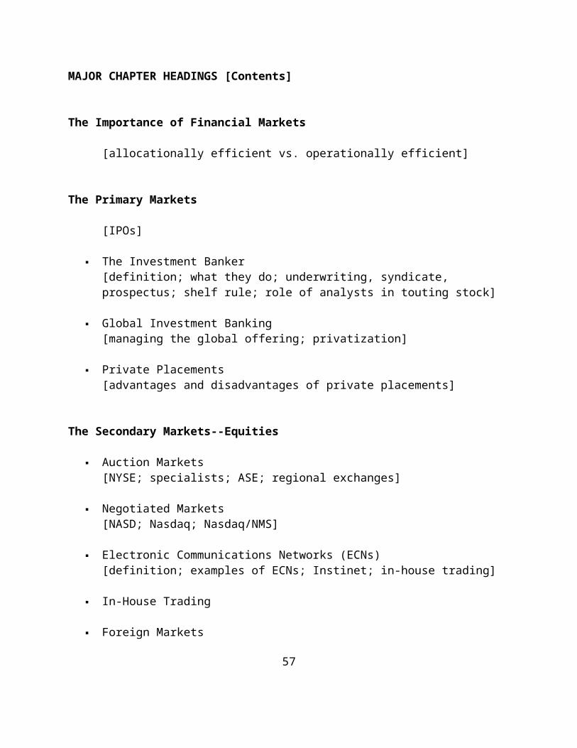
The Importance of Financial Markets
[allocationally efficient vs. operationally efficient]
The Primary Markets
[IPOs]
The Investment Banker[definition; what they do; underwriting, syndicate, prospectus; shelf rule; role of analysts in touting stock]
Global Investment Banking[managing the global offering; privatization]
Private Placements[advantages and disadvantages of private placements]
The Secondary Markets--Equities
Auction Markets [NYSE; specialists; ASE; regional exchanges]
Negotiated Markets[NASD; Nasdaq; Nasdaq/NMS]
Electronic Communications Networks (ECNs)[definition; examples of ECNs; Instinet; in-house trading]
In-House Trading
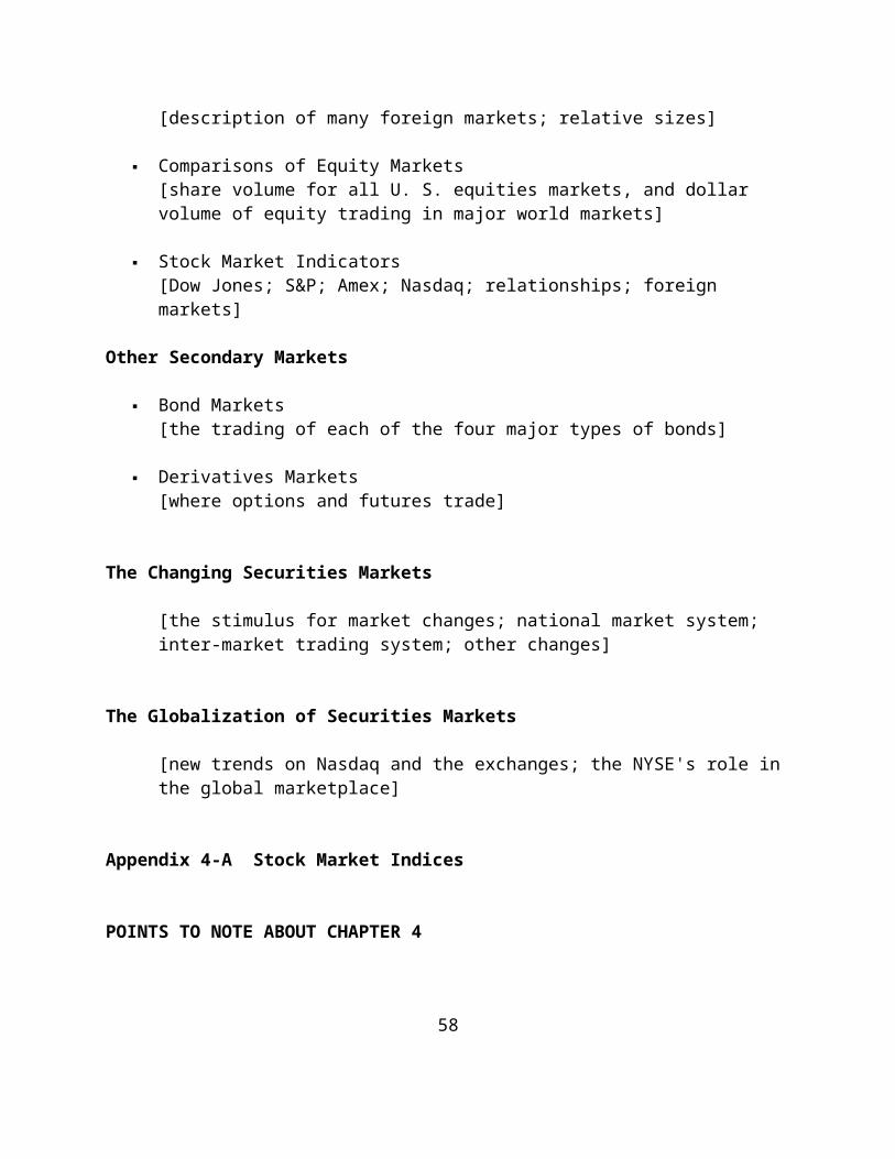
Foreign Markets[description of many foreign markets; relative sizes]
Comparisons of Equity Markets[share volume for all U. S. equities markets, and dollar volume of equity trading in major world markets]
Stock Market Indicators
56
[Dow Jones; S&P; Amex; Nasdaq; relationships; foreign markets]
Other Secondary Markets
Bond Markets[the trading of each of the four major types of bonds]
Derivatives Markets [where options and futures trade]
The Changing Securities Markets
[the stimulus for market changes; national market system; inter-market trading system; other changes]
The Globalization of Securities Markets
[new trends on Nasdaq and the exchanges; the NYSE's role in the global marketplace]
Appendix 4-A Stock Market Indices
POINTS TO NOTE ABOUT CHAPTER 4
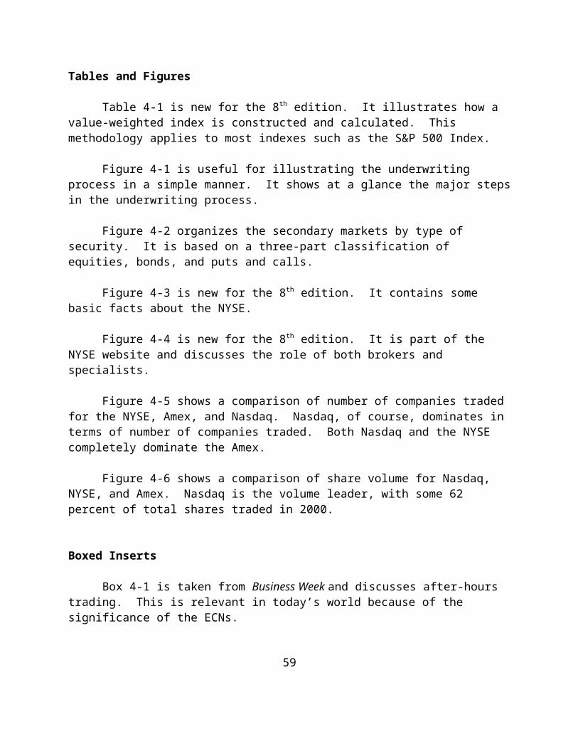
Tables and Figures
Table 4-1 is new for the 8th edition. It illustrates how a value-weighted index is constructed and calculated. This methodology applies to most indexes such as the S&P 500 Index.
Figure 4-1 is useful for illustrating the underwriting process in a simple manner. It shows at a glance the major steps in the underwriting process.
Figure 4-2 organizes the secondary markets by type of security. It is based on a three-part classification of equities, bonds, and puts and calls.
57
Figure 4-3 is new for the 8th edition. It contains some basic facts about the NYSE.
Figure 4-4 is new for the 8th edition. It is part of the NYSE website and discusses the role of both brokers and specialists.
Figure 4-5 shows a comparison of number of companies traded for the NYSE, Amex, and Nasdaq. Nasdaq, of course, dominates in terms of number of companies traded. Both Nasdaq and the NYSE completely dominate the Amex.
Figure 4-6 shows a comparison of share volume for Nasdaq, NYSE, and Amex. Nasdaq is the volume leader, with some 62 percent of total shares traded in 2000.
Boxed Inserts
Box 4-1 is taken from Business Week and discusses after-hours trading. This is relevant in today’s world because of the significance of the ECNs.
58
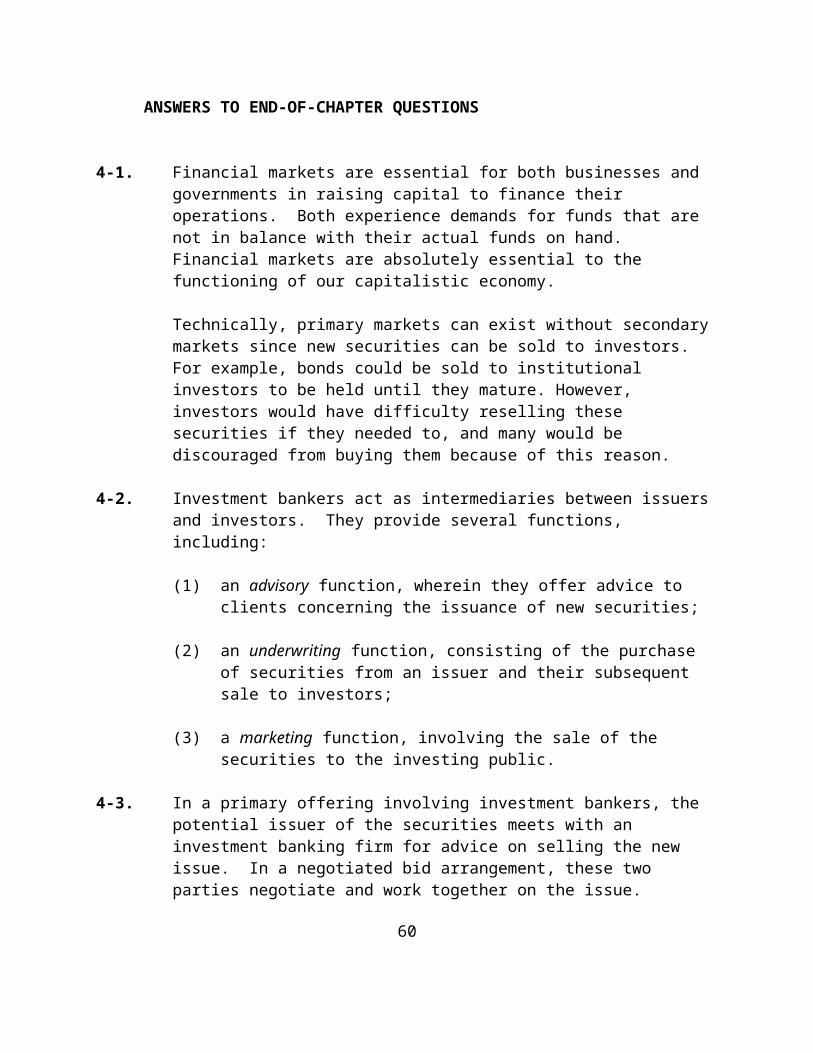
ANSWERS TO END-OF-CHAPTER QUESTIONS
4-1. Financial markets are essential for both businesses and governments in raising capital to finance their operations. Both experience demands for funds that are not in balance with their actual funds on hand. Financial markets are absolutely essential to the functioning of our capitalistic economy.
Technically, primary markets can exist without secondary markets since new securities can be sold to investors. For example, bonds could be sold to institutional investors to be held until they mature. However, investors would have difficulty reselling these securities if they needed to, and many would be discouraged from buying them because of this reason.
4-2. Investment bankers act as intermediaries between issuers and investors. They provide several functions, including:
(1) an advisory function, wherein they offer advice to clients concerning the issuance of new securities;
(2) an underwriting function, consisting of the purchase of securities from an issuer and their subsequent sale to investors;
(3) a marketing function, involving the sale of the securities to the investing public.
4-3. In a primary offering involving investment bankers, the potential issuer of the securities meets with an investment banking firm for advice on selling the new issue. In a negotiated bid arrangement, these two parties negotiate and work together on the issue. Subsequently, the investment banker, working with other investment banking firms (i.e., a syndicate), underwrites the issue; that is, the investment bankers purchase the securities from the issuer, thereby assuming the risk involved in actually selling the securities. After all legal requirements have been met (e.g., the issue is registered with the SEC), the selling group sells the
59
securities to the public via brokers who contact their customers about the issue.
4-4. The equity markets in the United States consist of the organized exchanges (the NYSE, the AMEX, and the regional exchanges) and the over- the-counter market.
• Auction markets, involving exchanges, include a bidding (auction) process in a specific physical location with brokers representing buyers and sellers.
• The over-the-counter market is a negotiated market, where dealers make the market in securities by standing ready to buy from, and sell to, investors based on bid-ask prices.
4-5. Commission brokers are members of brokerage houses with memberships on exchanges. They act as brokers for customers. Investment bankers act as middlemen between the issuers of the securities and the purchasers, in the same way that brokers do. Some firms offer both investment banking and retail brokerage services.
4-6. Specialists are members of exchanges who are assigned to particular stocks on an exchange. They are charged by the exchange with maintaining a continuous, orderly market in their assigned stocks. They do this by going against the market, buying (selling) when the public is selling (buying).
Specialists act as brokers by executing orders for other brokers for a commission. They act as dealers by buying and selling specific stocks for their own accounts.
4-7. Specialists should be, and are, closely monitored and regulated. Because they maintain the limit books, they have knowledge of all limit orders on either side of the current market price. They are charged with acting for the public interest by maintaining an orderly market; simultaneously, they buy and sell for their own accounts in hopes of profiting from the spread between purchases and sales. Clearly, specialists must be closely regulated because of these potentially conflicting roles.
60
4-8. A specialist on the exchange often acts as a dealer, buying and selling for his or her own account. This is exactly what an OTC dealer does.
4-9. NASD stands for the National Association of Security Dealers, a self- regulating body of brokers and dealers that oversees OTC practices. NASD licenses brokers and handles the punishment for violators of its prescribed fair practices.
Nasdaq is the acronym for the NASD Automated Quotation System, a computerized communications network providing current bid-ask prices for thousands of OTC stocks simply by pressing buttons on a terminal.
4-10. The third market involves OTC transactions in securities listed on the organized exchanges.
The fourth market involves direct transactions among large institutions, bypassing intermediaries such as brokers and dealers.
4-11. The two primary factors accounting for the rapid changes in U.S. securities markets are:
(1) Pressure by institutional investors, who have emerged as the dominant force in the market.
(2) The Securities Acts Amendments of 1975, which called for a national market system.
4-12. The NYSE has favored the ITS system because NYSE brokers can ignore better quotes on other exchanges. The system does not guarantee that orders will be routed to the exchange offering the best price.
4-13. Investors have become increasingly interested in equity markets around the world because the United States now accounts for only about one-third of the world's stock market capitalization. Many equity markets exist. Examples in the developed countries include the United Kingdom, France, Germany, Italy, Switzerland, Japan, Hong Kong, and Canada. U.S. investors are also interested in the stock markets of emerging countries such as Mexico, Brazil, and Indonesia. Based on the dollar volume of
61
equity trading in major world markets for the year 1995 the NYSE dominated, followed by Nasdaq, London, and Tokyo.
NASD members in the United Kingdom can use Nasdaq as if they were located in this country. The Nasdaq International Market started in 1991, trading OTC stocks early in the morning during regular trading hours in London. Although the NYSE has already traded several hundred foreign stocks, it would like to trade hundreds more in order not to become a “regional exchange” in the global marketplace.
4-14. The Nasdaq National Market System combines the system of competitive multiple market makers in the OTC market with the continuous reporting of trades found on the organized exchanges. The conventional OTC market has multiple dealers, but stocks are reported on a bid-ask basis.
The Nasdaq/NMS could be a prototype for the future structure of a national market system. It would appear to combine the best elements from the organized exchanges and the OTC market, but in terms of execution the issue is unsettled. An auction market such as the NYSE also offers advantages.
4-15. The Dow-Jones Industrial Average is a price-weighted average of 30 large (blue-chip stocks) trading on the NYSE. The S&P 500 Composite Index is a market value index consisting of 500 stocks, with a base period set to 10 (1941-1943).
These measures are the two most often-used indicators of what stocks in general are doing. The Dow-Jones Averages are carried by The Wall Street Journal, while the S&P 500 Index is the indicator most often used by institutional investors.
4-16. Blue chip stocks are large, well-established and well-known companies with long records of earnings and dividends. They are typically traded on the NYSE. Examples include Coca-Cola, General Electric, Merck, Philip Morris, and IBM (despite any recent problems).
62
4-17. The EAFE Index, or the European, Australia, and Far East Index, is a value-weighted index of the equity performance of major foreign markets. It is, in effect, a non-American world index.
4-18. Blocks are defined as transactions involving at least 10,000 shares. Large-block activity on the NYSE is an indicator of institutional investor participation in equity trading. The total number of large-block transactions has increased over the years on the NYSE, with an average of 13,961 blocks changing hands daily by the end of 1998. Block volume accounted for about 49 percent of the NYSE’s reported volume at the end of 1998, amounting to some 83 billion shares.
4-19. The NYSE’s role in global trading will depend on several events. The NYSE position is that investors need a public auction market. Another important variable is the listing of big foreign stocks on the NYSE. About half of the foreign listings on the NYSE occurred only in the last few years. The NYSE wants to list more, but the SEC has been reluctant because of accounting differences between countries.
4-20. Instinet, a part of the fourth market, is an electronic trading network that handles a few billion shares each year. It allows institutions to trade among themselves. Brokers can use Instinet to trade Nasdaq stocks, thus taking business from dealers in that market.
4-21. In-house trading refers to internal trading by fund managers within one company without the use of a broker or an exchange. Traders agree to buy and sell in-house, or cross-trade, perhaps at the next closing price. Fidelity Investments operates an in-house trading system for its own funds because of the large amount of buying and selling it does every day. Large international investors will benefit from in-house trading.
4-22. Although a few bonds trade on the NYSE and ASE, the bond market is primarily an OTC market. All federal, agency, and municipal bonds trade OTC, and most corporates.
4-23. Growth stocks are the most likely stocks to split. As high-priced stocks split and their prices decline, they
63
lose relative importance in the DJIA, which is a price-weighted series. High-price stocks carry more weight than do low-priced stocks in such a series.
4-24. Institutional investors have become increasing important on Nasdaq. For Nasdaq national market stocks, by 1997 institutions accounted for about 48 percent of shares held as well as for about 48 percent of the market value of holdings.
4-25. Merrill Lynch acts as the lead investment banker in bringing out a new issue, or IPO. In effect, Merrill Lynch (and the syndicate, if any) purchases the securities from the issuer and resell them to the public, hoping to profit by the spread between the two prices. It assumes the risk involved in adverse price movements.
Chapter 5: How Securities Are Traded
CHAPTER OVERVIEW
Chapter 5 allows students to concentrate solely on the mechanics of securities trading after learning about financial markets in Chapter 4. This material typically is of great
64
interest to most students, and instructors must decide how much time and effort to devote to it.
Chapter 5 devotes considerable attention to the major aspects of brokerage transactions. An important part of this discussion centers around brokers themselves, a subject which tends to interest many students quite a lot. The chapter discussion explains what brokers do, the types of brokerage operations (full-service vs. discount vs. deep discount), how brokers are compensated, and how much they make annually.
The remainder of the brokerage transaction discussion covers the major points that students need to know. These include the types of brokerage accounts, commissions, investing without a broker, how orders work, the types of orders, clearing procedures, using the internet, and so forth. Instructors will wish to vary their discussions of this material depending upon student knowledge, interest, time availability, and current discussions in the popular press.
There are numerous interesting illustrations that can be given of brokerage costs, how orders work on the exchanges and in the OTC, market orders versus limit orders, and so forth. The popular press regularly has articles that would be appropriate for class discussion, including Smart Money, Worth, Forbes, Business Week, and Financial World.
Chapter 5 contains a thorough discussion of investor protection in the markets, a topic of concern to many investors. This covers not only federal legislation and the SEC but also self-regulation by the stock exchanges, including the latest measures on the NYSE such as trading halts and sidecars. The role of the NASD in regulating brokers and dealers also is covered. An extended example of regulation involving penny stocks is given.
The remainder of the chapter is devoted to margin trading and short selling. These are important subjects, and ones that many students have difficulty understanding, particularly short selling. It is suggested that instructors spend a reasonable amount of time explaining these concepts.
CHAPTER OBJECTIVES
65
To provide students with a good understanding of what brokers do, how securities are traded, and so forth as a natural extension of the discussion of financial markets in Chapter 4.
To explain the mechanics of securities trading, such as brokerage transactions, margin trading, and short selling.
To provide an overview of how markets are regulated without simply describing the various federal acts.
66
MAJOR CHAPTER HEADINGS [Contents]
Brokerage Transactions
Brokerage Firms[full-service brokers, discount brokers, how brokers earn their income, examples of discount brokers]
Types of Brokerage Accounts[cash vs. margin, asset management account, wrap account]
Commissions[negotiated rates; examples]
Investing Without a Broker[dividend reinvestment plans; direct stock purchase programs]
How Orders Work
Orders on the Organized Exchanges[how orders work on the NYSE; specialists; automation on the NYSE]
Orders In The Over-The-Counter Market[bid price and asked price]
Decimalization of Stock Prices[NYSE and Nasdaq convert to decimals]
Types of Orders[market, limit, stop]
Clearing Procedures[settlement date; street name; clearing houses]
Investor Protection In The Securities Markets
Government Regulation[Federal legislation; the SEC; insider trading]
67
Self-Regulation[regulation by the NYSE--trading halts, sidecars, Rule 80A; the role of the NASD]
Other Investor Protections[Securities Investor Protection Corporation (SIPC); arbitration]
One Example of Regulation--The Case of Penny Stocks
Margin
[definition; types; margin calls; examples]
Short Sales
[definition; examples; details of short selling]
Appendix 5-A The Details of Margin Accounts
POINTS TO NOTE ABOUT CHAPTER 5
Tables and Figures
Table 5-1 outlines the details on types of orders: market, limit and stop orders. The intent is to present this material in a concise format, and illustrate it with examples.
Table 5-2 contains a brief description of the major legislative acts regulating the securities markets. This material can be very tedious when presented as regular text. This presentation better allows instructors to devote as much, or as little, time as they desire.
Table 5-3 presents the details of short selling. Such details are important, and this presentation helps to keep these details from being “lost”.
68
Box Inserts
There are no boxed inserts for this chapter.
69
ANSWERS TO END-OF-CHAPTER QUESTIONS
5-1. A market order ensures that a customer’s order will be executed quickly, at the best price the broker can obtain. Thus, an investor who wants to be certain of quickly establishing a position in a stock (or getting out of a stock) will probably want to use a market order.
A limit order specifies a particular price to be met or bettered. The purchase or sale will occur only if the broker obtains that price, or betters it. Therefore, an investor can attempt to pay no more than a certain price in a purchase, or receive no less than a certain price in a sale; a completed transaction, however, cannot be guaranteed.
A stop order specifies a certain price at which a market order takes effect. The exact price specified in the stop order is not guaranteed, and may not be realized.
Limit orders are placed on opposite sides of the current market price of a stock from stop orders. For example, while a buy limit order would be placed below a stock’s current market price, a buy stop order would be placed above its current market price.
5-2. Most securities are sold on a regular way basis, meaning the settlement date is three business days after the trade date. The three-day settlement period--T+3--took effect in mid-1995.
5-3. By keeping their securities in a street name, investors transfer the safekeeping function to their brokers; furthermore, upon sale they do not have to worry about delivering the securities to the broker.
Possible disadvantages include the financial failure of the brokerage house, resulting in at least a temporary tie-up of the securities. Also, an investor may wish to use securities for collateral, and it can take weeks to have them delivered from a street name.
5-4. Margin is the equity that a customer has in a transaction. The Board of Governors of the Federal Reserve System sets the initial margin, which is the
percentage of the value of a securities transaction that the purchaser must pay at the time of the transaction. The purchaser then borrows the remainder from the broker, traditionally paying as interest charges the broker loan rate plus 1-2% (approximately). Completion, however, may result in significantly different rates paid by the customer.
In addition to the initial margin, all exchanges and brokers require a maintenance margin below which the actual margin cannot go (this is typically 30% or more).
5-5. Actual margin between the initial and maintenance margins results in a restricted account where no additional margin purchases are allowed.
If the actual margin declines below the maintenance margin, a margin call results, requiring the investor to put up additional cash or securities (or be sold out by the brokerage firm).
5-6. If an investor sells short, he or she is (usually) selling a security that is not owned. The broker borrows the security from another customer (who owns it), and lends it to the short seller who must subsequently replace it. In effect, the investor from whom the security is borrowed never knows it since his or her monthly statement continues to reflect a long position.
5-7. Short sales on the exchanges are permitted at the last trade price only if that price exceeded the last different price before it. Otherwise, the seller must wait for an uptick. This restriction does not apply to OTC stocks.
5-8. A sell limit order and a buy stop order are above the current market price.
A buy limit order and a sell stop order are below the current market price.
5-9. The margin requirement for U. S. government securities is 10 percent or less.
5-10. With a wrap account, investors with large sums to invest use a broker as a consultant to choose an outside money
manager from a list provided by the broker. All costs are wrapped in one fee--the cost of the broker-consultant, the money manager, and transactions costs. For stocks, a typical fee is 3% of the assets managed (and less for larger accounts).
5-11. A discount broker offers reduced brokerage commissions relative to full-service brokers such as Merrill Lynch but also offers most of the same services, the exception being research reports and recommendations/advice. Large discount brokers include Fidelity, Charles Schwab, and Quick and Reilly. Investors can visit an office, call a broker at one of these firms, or use their internet facilities.
Deep-discount brokers offer bare-bones brokerage commissions but little else. These firms tend to be quite small and provide services primarily over the internet.
5-12. More than 800 companies offer dividend reinvestment plans, whereby dividends can be used to purchase additional shares of the company paying the dividend.
Many companies now offer direct purchase stock plans, allowing investors to purchase shares directly from the company. Exxon is a good example. Investors can open a direct-purchase account with Exxon to buy its stock.
5-13. The role of specialists is critical on an auction market such as the NYSE. They are expected to maintain a fair and orderly market in those stocks assigned to them, often going against the market.
As brokers, specialists maintain the limit book, which records all limit orders. The commission brokers leave the limit orders with the specialist to be filled when possible, paying a specialist a fee to do this.
As dealers, specialists buy and sell shares of their assigned stocks to maintain an orderly market. The specialist will buy from commission brokers with orders to sell and sell to those with orders to buy, hoping to profit by a favorable spread between the two sides.

5-14. SuperDot is an electronic order routing system for NYSE-listed securities. Member firms send orders directly to the specialist post where the securities are traded and confirmation of trading is returned directly to the member firm over the same system. The system has order processing capacity of 800 million shares a day. SuperDot also includes components to handle both preopening buy and sell orders and postopening market orders.
5-15. Both of these terms apply to limit orders. An open order remains in effect for six months unless canceled or renewed. A day order is effective for only one day.
5-16. The mission of the SEC is to administer laws in the securities field and to protect investors and the public in securities transactions. In general, it administers all securities laws.
5-17. The National Association of Securities Dealers (NASD) regulates brokers and dealers. All brokers must register with the NASD in order to trade securities. The NASD can bar individuals from association with any NASD member; having done so, it has no jurisdiction over the individual. The NASD can fine an individual. Penalties can be appealed to the SEC, which suspends the monetary penalties until resolution.
5-18. Investors are interested in margin accounts because such accounts permit the magnification of gains (but also losses). With a margin requirement of 50%, percentage gains are doubled (ignoring transaction costs and interest costs) because the investor only has 50% of the value of the transaction at stake; that is, his or her own equity is only 50% of the value of the transaction.
The risks are obvious. If the transaction goes against the investor, the percentage losses are doubled, and interest costs must still be paid.
Investors are required to have margin accounts for some transactions, such as short sales.
5-19. Short sales account for approximately 9 percent of all reported sales. The public accounts for about one third
of short sales on the NYSE, with NYSE members accounting for about two-thirds.
5-20. The basis of regulation of mutual funds is the Investment Company Act of 1940. This federal act has been incredibly successful in regulating the investmentcompany industry, providing almost total confidence in investors as to the operations of investment companies.
5-21. The Investors Advisors Act of 1940 simply requires would-be investment advisors to fill out a form and pay a fee to register with the SEC. There are no education or competency requirements. Therefore, investors have no assurances as to the abilities of people offering advice.
5-22. The NYSE has established certain trigger points referred to as “circuit-breakers” that are designed to reduce market volatility. Rule 80B was revised in 1998. Trigger levels are now set at 10%, 20%, and 30% of the DJIA, calculated at the beginning of each quarter. Trading halts of one hour and two hours are associated with the 10% and 20% declines (but vary depending upon time of day). A decline of 30% closes the market for the rest of the day.
5-23. Investors may choose to use a full-service broker for several reasons. First, they may have confidence in a particular broker and wish to have the personal contact implied in such a relationship. Second, they can seek, and obtain, advice from the broker, and by extension, the entire resources of a firm such as Merrill Lynch. Third, they can obtain considerable research reports and investing information, which are often extensive in nature. Fourth, full-service brokers may offer a wider range of services than many discount brokers, and investors needing such services will want to have them available.
5-24. The SEC does not provide assurances to investors when an IPO is marketed in terms of being able to tell investors that the company will be successful. The SEC does ensure that the company selling the new securities has complied with various accounting and legal provisions, thereby hopefully preventing the sale of new securities based upon fraudulent or misleading information.
5-25. The specialist system on the exchanges assigns stocks to specialist firms, who then make a market in the stock. Specialists buy from and sell to the public to maintain an orderly market in the stock. The system has worked well over the years, and has provided some notable successes in maintaining orderly markets. For example, in the great crash of October 19, 1987, specialists remained at their posts, trading stocks and providing liquidity.
Dealers in the over-the-counter market make markets in stocks, buying from investors and selling to them from their inventory. Thus, they have a vested interest in each transaction, and in the spread between the bid and asked price. Investigations in the 1990s revealed that these spreads often were too wide relative to what should be expected. In many cases, these spreads have narrowed since these investigations.
ANSWERS TO END-OF-CHAPTER PROBLEMS
5-1. (a) A limit order to sell is placed above the current market price. If the limit order is set at $130, the investor will realize a gross profit of at least $30 (ignoring transaction costs).
(b) A sell stop order is placed below the market price. If the stop order is placed at $120, the investor should realize a profit of approximately $20 per share. Technically, to be certain of $20 per share, the stop order probably would have to be set slightly above $120 because a stop price is actually an activator that initiates a market order when the specified price is reached.
5-2. To realize a gross profit of $5000 on 200 shares sold short at $75, the investor must cover at (ignoring transaction costs):
200($75) = $15,000 - X ─────── = $ 5000 profit
X is $10,000, which must be divided by 200 shares.
ANSWER: $50 per share
For a profit of $1000, the calculation is:
$15,000 - X ─────── $ 1000
X is $14,000, which again must be divided by 200 shares.
ANSWER: $70 per share.
5-3. 100 shares at $50 per share is a total cost of $5000. At 50% margin, the investor must put up $2500, resulting in a gross profit percentage relative to equity of
63
$1000/$2500 = 40%
At 40% margin, the investor must put up $2000, resulting in a gross profit percentage relative to equity of
$1000/$2000 = 50%
At 60% margin, the investor must put up $3000, resulting in a gross profit percentage relative to equity of
$1000/$3000 = 33.3%
5-4. The initial margin is 50% of $6000, or $3000. The other $3000 is borrowed from the broker.
(a)
market value of securities - amount borrowedactual margin = ──────────────────────────────────────────── market value of securities
$5000 - $3000 = ───────────── $5000 = 40%
(b) In a restricted account, the actual margin is between the initial margin (i.e., 50%) and the maintenance margin (i.e., 30%). The actual margin is now:
market value of securities - amount borrowed actual margin = ──────────────────────────────────────────── market value of securities
$5500 - $3000 = ───────────── $5500
= 45.5%
Therefore, the account is restricted.
64
(c) A margin call results when the actual margin declines below the maintenance margin. At a stock price of $49, the actual margin is:
$4900 - $3000 actual margin = ───────────── $4900 = 38.8%
Because the actual margin is not below the maintenance margin of 30%, there is no margin call.
(d) At a stock price of $45, the actual margin is
$4500 - $3000 actual margin = ───────────── $4500
= 33.3%
There is no margin call at a price of $45.
At $35, however, the actual margin is
$3500 - $3000 actual margin = ───────────── $3500
= 14.3%
The amount of the margin call is calculated as:
(x + $3500) - $3000.3 = ----------------------
(x + $3500)
= $785.71
5-5. a) The margin requirement is 55%.
65
Amount put up = .55 x 28,600 = $15,730
Amount borrowed = .45 x 28,600 = $12,870
Gross profit = $28,600 - $5,400 = $23,200
Net Profit = $23,200 – [$12,870 x .09] - $40 = $22,001.70Gross pr.-Int. costs- 2 way transactions costs
b) initial investment = $15,730 + $20 = $15,750
% return on investment = $22,001.70 / $15,750= 1.397, or 140% return (rounded)
5-6. a) initial cost of 100 shares = $15,600 + $20.
Initial investment put up by investor buying on 60% margin = .6 ($15,600) = $9,360
Initial cost = 9,360 + 20 = 9,380
Margin cost for one year=$6,240 x .09 =$561.60
Dollar gain = $23,300 – $15,600 - $561.60 + 130 -$40
= $7,228.40
b) % return on investment = $7,228.40/$9,380=77%
66
Chapter 6: The Returns and Risks From Investing
CHAPTER OVERVIEW
The purpose of Chapter 6 is to present an analysis of risk and return early enough in the text for these concepts to be used throughout the book. Return and risk are the key elements of investment decisions--in effect, everything else revolves around these two factors. It makes sense, therefore, to analyze and discuss these concepts in detail.
Chapter 6 focuses only on understanding and measuring realized returns and wealth. This allows students to concentrate on this one issue, in a comprehensive manner. All of the equations for calculating various types of returns are included in this chapter, providing a complete package in this regard. It is doubtful that beginning students could need any more than what is contained here with regard to realized returns.
Chapter 6 provides a complement to Chapter 7, which covers expected returns and risk and the basic calculations of portfolio theory. Thus, in Chapter 6 we analyze and calculate realized returns, while in Chapter 7 we analyze and calculate expected returns, based on probability distributions.
This discussion centers around the definition and meaning of return and risk, including the components of return, the sources of risk, and types of risk. The emphasis is on how to both understand and measure return and risk. Considerable attention is devoted to explaining the total return (TR), return relative (RR), and cumulative wealth calculations, which are used throughout this text and are exactly comparable to the definitions used in such prominent sources as the Ibbotson Associates Yearbook. Numerous examples of these important calculations are presented.
The discussion of returns measures facilitates the presentation of the data on rates of return and wealth indexes. This data is both important (as benchmarks) and interesting (it can be the basis of lively class discussion). The data used here
67
were collected and calculated by the author, and correspond closely with the Ibbotson data.
The use of the geometric mean is fully explored, along with wealth indexes. Calculations include measuring the yield component and capital gains component of total returns and cumulative wealth separately, measures of inflation-adjusted returns, and risk premiums.
Definitions of risk are presented and discussed. Examples include calculations involving the standard deviation. The breakdown of total risk into a systematic part and a nonsystematic part is introduced in Chapter 6 to facilitate the discussion of market risk, portfolio diversification, and so forth. These concepts are treated in more detail in Chapter 7, and in Chapters 19 and 20.
This chapter contains an extensive problem set.
CHAPTER OBJECTIVES
To explain the meaning and measurement of both return and risk.
To illustrate the use of such measures as the geometric mean and standard deviation.
To present the well-known Ibbotson data on rates of return.
To present and illustrate virtually all the calculations needed for a thorough understanding of return and risk.
68
MAJOR CHAPTER HEADINGS [Contents]
Return
The Components of Return[Yield; Capital gain/loss; total return = the sum of these two]
Risk
Sources of Risk[sources include: interest rate; market; inflation; business; financial; liquidity; exchange rate; country]
Types of Risk[total risk can be divided into nonsystematic risk and systematic risk]
Measuring Returns
Total Return[definition; examples]
Return Relative[definition; example]
Cumulative Wealth Index[definition; index]
Taking a Global Perspective
[definition; index]
International Returns and Currency Risk[calculating foreign returns to U.S. investors]
Summary Statistics for Returns[arithmetic mean; geometric mean; comparisons]
Inflation-Adjusted Returns[definition; calculations]
69
Measuring Risk
Standard Deviation[definition; formula; example]
Risk Premiums[definition; equity risk premium; maturity premium]
Realized Returns And Risk From Investing
Total Returns and Standard Deviations[linkage between arithmetic and geometric mean; data on rates of return for major asset classes]
Cumulative Wealth Indexes[cumulative wealth figure; inflation-adjusted cumulative wealth; the yield and price change components of cumulative wealth]
POINTS TO NOTE ABOUT CHAPTER 6
Tables and Figures
Exhibit 6-1 should be reviewed carefully with students as examples of how to calculate total returns and return relatives for three different securities.
Table 6-1 shows annual S&P 500 data--prices and dividends--from 1919 through the latest year possible. Calculated total returns for each year are presented. This table provides a good source of data for discussions throughout the text involving market returns as measured by the S&P 500 Index. These data were calculated and compiled by Jack Wilson and Charles Jones.
Tables 6-2 and 6-3 involve the calculation and interpretation of the arithmetic and geometric means using TRs. It is suggested that instructors stress the meaning of the geometric mean.
Table 6-4 (for historical data) shows calculations for the standard deviation and can be handled by students on their own or
70

emphasized by instructors to the extent thought necessary.
Table 6-5 is an important table on rates of return and should be used as a transparency for class discussion. This table is important for numerous reasons: investors need to know the historical return series for benchmark purposes, it illustrates the nature of the return--risk tradeoff, and it allows you to talk about the variability in returns over time by analyzing the arithmetic and geometric means as well as the standard deviations presented in the table. In addition, other points can be developed, such as the “small” stock effect, and so forth.
NOTE: This table corresponds quite well with the comparable table from Ibbotson Associates. Key differences include a start date at the end of 1919, and the use of 500 stocks instead of 90 stocks (which Ibbotson Associates uses) for a number of years.
Figure 6-1 shows the spread in returns for the major financial assets covered in Table 6-5. As we would expect, both stock categories have wider spreads than do bonds, and small stocks have a wider dispersion than does the S&P 500.
Figure 6-2 shows cumulative wealth indices for the major financial assets since 1919 and is a good source of class discussion because students find this interesting. Instructors may wish to emphasize how these values are calculated (which is covered in the chapter).
Box Inserts
Box 6-1 is an interesting discussion from Business Week about the equity risk premium. The discussion concerns what the equity risky premium is, how to measure it, and what the controversy is all about. This boxed insert can provide a basis for good class discussion.
71
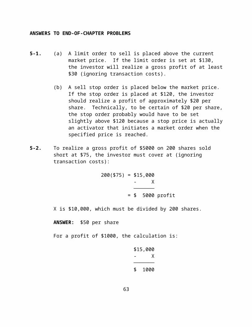
ANSWERS TO END-OF-CHAPTER QUESTIONS
6-1. Historical returns are realized returns, such as those
reported by Ibbotson Associates.
Expected returns are ex ante returns--they are the most likely returns for the future, although they may not actually be realized because of risk.
6-2. A Total Return can be calculated for any asset for any holding period. Both monthly and annual TRs are often calculated, but any desired period of time can be used.
6-3. Total return for any security consists of an income (yield) component and a capital gain (or loss) component. • The yield component relates dividend or interest
payments to the price of the security.
• The capital gain (loss) component measures the gain or loss in price since the security was purchased.
While either component can be zero for a given security over a specified time period, only the capital change component can be negative.
6-4. TR, which is another name for holding period yield, is a percentage return, such as +10% or -15%. The term “holding period return” is sometimes used instead of TR.
Return relative adds 1.0 to the TR in order that all returns can be stated on the basis of 1.0 (which represents no gain or loss), thereby avoiding negative numbers so that the geometric mean can be calculated).
6-5. The geometric mean is a better measure of the change in wealth over more than a single period. Over multiple periods the geometric mean indicates the compound rate of return, or the rate at which an invested dollar grows, and takes into account the variability in the returns.
The geometric mean is always less than the arithmetic mean because it allows for the compounding effect--the earning of interest on interest.
72
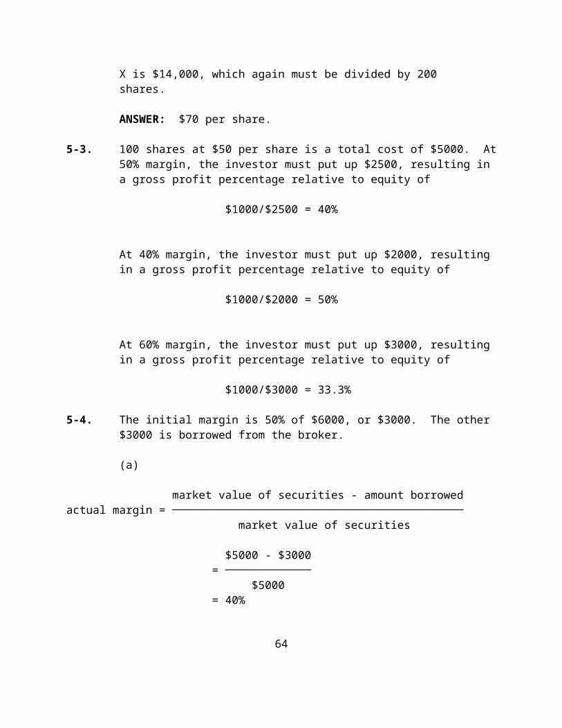
6-6. The arithmetic mean should be used when describing the average rate of return without considering compounding. It is the best estimate of the rate of return for a single period. Thus, in estimating the rate of return for common stocks for next year, we use the arithmetic mean and not the geometric mean. The reason is that because of variability in the returns, we will have to average the arithmetic rate in order to achieve a rate of growth which is given by the smaller geometric mean.
6-7. See Equation 6-14. Knowing the arithmetic mean and the standard deviation for a series, the geometric mean can be approximated.
6-8. An equity risk premium is the difference between stocks and a risk-free rate (proxied by the return on Treasury bills). It represents the additional compensation, on average, for taking the risk of equities rather than buying Treasury bills.
6-9. As Table 6-5 shows, the risk (standard deviation) of all common stocks for the 1920-2000 period was 20.7%, about two and one-half times that of government and corporate bonds. Therefore, common stocks are clearly more risky than bonds, as they should be since larger returns would be expected to be accompanied by larger risks over long periods of time.
6-10. Market risk is the variability in returns due to fluctuations in the overall market. It includes a wide range of factors exogenous to securities themselves.
Business risk is the risk of doing business in a particular industry or environment. Interest rate risk and inflation risk are clearly directed related. Interest rates and inflation generally rise and fall together.
6-11. Systematic risk: market risk, interest rate risk, inflation risk, exchange rate risk, and country risk.
Nonsystematic risk: business risk, financial risk, and liquidity risk.
6-12. Country risk is the same thing as political risk. It refers to the political and economic stability and
73
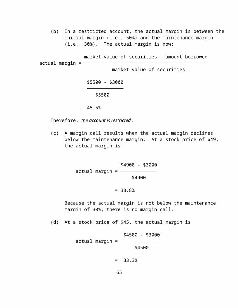
viability of a country’s economy. The United States can be used as a benchmark with which to judge other countries on a relative basis.
Canada would be considered to have relatively low country risk although some of the separation issues that have occurred there have probably increased the risk for Canada. Mexico seems to be on the upswing economically, but certainly has its risk in the form of nationalized industries, overpopulation, and other issues. Mexico also experienced a dramatic devaluation of the peso.
6-13. The return on the Japanese investment is now worth lessin dollars. Therefore, the investor’s return will be less after the currency adjustment.
EXAMPLE: Assume an American investor on the Japanese market has a 30% gain in one year but the Yen declines in value relative to the dollar by 10%. The percentage of the original investment after the currency risk is accounted for is (0.9)(130%) = 117%. Therefore, the investor’s return is 17%, not 30%. In effect, the investor loses 10% on the original wealth plus another 10% on the 30% gain, or a total of 13 percentage points of the before-currency-adjustment wealth of 130% of investment.
6-14. Risk is the chance that the actual outcome from an investment will differ from the expected outcome. Risk is often associated with the dispersion in the likely outcomes. Dispersion refers to variability, and the standard deviation is a statistical measure of variability or dispersion.
Standard deviation measures risk in an absolute sense.
Beta is a relative measure of the risk of an individual security in relation to the overall market, which has a beta of 1.0. Betas have intuitive meaning only in relation to the benchmark of 1.0 for the market beta.
6-15. A wealth index measures the cumulative effect of returns over time, typically on the basis of $1 invested. It measures the level rather than changes in wealth.
74

The geometric mean is the nth root of the wealth index. Alternatively, adding 1.0 to the decimal value of the geometric mean and raising this number to the nth power produces the ending wealth index.
6-16. You cannot validly compare a 79-year mean return with recent return figures because of inflation premiums. The expected return on common stocks may be higher than the historical realized mean because of a higher inflation premium (at a minimum). The proper comparison is either between the historical returns on both stocks and bonds or the current expected returns on both stocks and bonds.
6-17. Dividing the geometric mean return for common stocks by the geometric mean for inflation for a given period produces the inflation-adjusted rate of return.
6-18. The two components of the cumulative wealth index are the yield (income) component and the price change (capital gain or loss) component. Multiplying these two components together produces cumulative wealth. Knowing one of these components, the other can be calculated by dividing the known component into the cumulative wealth index number.
6-19. No. These relationships are not linear, nor is there any reason why they should be. The risk on common stocks relative to bonds has been more than twice as great.
6-20. This means that a loss occurred. An index number less than 1.0 connotes a loss. The capital gain component for bonds over very long periods of time has, in fact, been less than 1.0, indicating a negative rate of return.
CFA6-21. Purchasing power risk is the risk of inflation reducing
the returns on various investments. One should look at the total return of equities on a price level adjusted basis.
Interest Rate Risk is a rise in the level of interest rates that depresses the prices of fixed income instruments and frequently causes lower prices for equities. Interest rate volatility and uncertainty are both relevant.
75
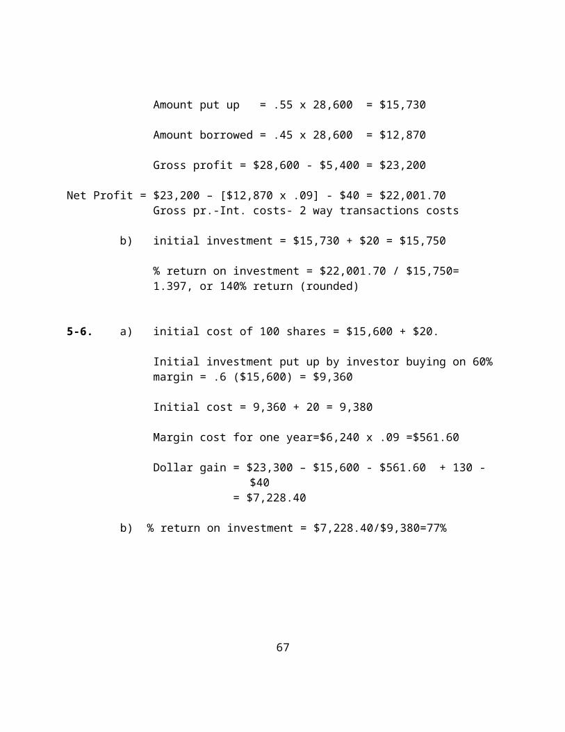
Business Risk includes the risks associated with the business cycle. Stock prices tend to go down in anticipation of a downturn in the business cycle. Factors affecting the business cycle include the impact of monetary policy, changes in technology, changes in supply of raw materials. Attempting to correctly forecast the turning point in a business cycle and the factors that affect a business cycle can reduce the business risk.
Market Risk is the general risk associated with fluctuations in the stock market. When the stock market declines, most stocks go down. While a low beta for a stock or a defensive stock position may reduce the volatility, the stock market has a pervasive influence on individual stocks.
Exchange rate risk is the potential decline in investment value due to a decline in the currency in which the shares or bonds are held.
Regulatory risk is the risk of an unanticipated change in the regulation of factors that affect investments such as changes in tax policy.
Political risk is the unanticipated change in investment environment due to a change in political parties or a change of view of the current political party.
76
ANSWERS TO END-OF-CHAPTER PROBLEMS
6-1. Using IBM data from Demonstration Problem 6-1:
Year capital gain total $ return (loss) 19X1 -$10.30 -$6.86 19X2 3.40 6.84 19X3 -11.00 -7.56 19X4 39.55 42.99 19X5 25.75 29.46
TR for 19X3 = ($3.44 + ($56.70 - $67.70))/$67.70
= -.1117 or -11.2%
TR for 19X4 = ($3.44 + ($96.25 - $56.70))/$56.70
= .7582 or 75.8%
NOTE: These two years (actual 1973 and 1974 returns) were chosen specifically for their contrast. This is a good opportunity for instructors to point out how TRs for even a blue chip company such as IBM have fluctuated violently from year-to-year. This shows dramatically the risk of common stocks as well as the opportunities for large returns.
6-2. This investor would have a (short-term) capital gain, with a tax liability of
$5000 - $4000 = $1000 (.28) = $280
6-3. Calculating Total Returns (TRs) for these assets:
(a) TRps = (Dt + (PE - PB))/PB
where Dt = the preferred dividend PE = ending price or sale price PB = beginning price or purchase price
TR = (5 + -7)/70 = -2.86%
84
(b) TRw = (Ct + PC)/PB
where Ct is any cash payments paid (there are none for a warrant)
PC = price change during the period
TR = (0 + 2)/11
= 18.18% for the three month period
(c) TRb = (It + PC)/PB
= (240* + 60)/870
= 34.5% for the two year period.
*interest received is $120 per year (12% of $1000) for two years.
Calculating Return Relatives (RRs) for these examples:
(a) a TR of -2.86% is equal to a RR of .9714 or (1.0+[-.0286])
(b) a TR of 18.18% is equal to a RR of 1.1818(c) a TR of 34.5% is equal to a RR of 1.345
6-4. Calculate future values using tables at end of text: @12%
$100 (1.762) = $176.20 after 5 years$100 (3.106) = $310.60 after 10 years$100 (9.646) = $964.60 after 20 years $100 (29.96) = $2996.00 after 30 years
Calculate present values using tables at end of text: @12%
$100 (.567) = $56.70 after 5 years$100 (.322) = $32.20 after 10 years$100 (.104) = $10.40 after 20 years $100 (.033) = $3.30 after 30 years
6-5. (a) The arithmetic rate of return is
85

[.3148 + (4.847) + 20.367 + 22.312 + 5.966 + 31.057]/6 = 17.72
The geometric mean rate of return for the S&P 500 Composite Index for 1980-1985 (from Table 6-1) is:
G = (1.3148 x .95153 x 1.20367 x 1.22312 x 1.05966 x 1.31057)1/6 - 1.0
= (2.5579111)1/6 - 1.0
= 1.1694 - 1.0 = .1694 or 16.94% 6-6. Refer to Equation 6-12 for the standard deviation formula.
We will use n-1 in the calculation.
Year TR(%),X X-X (X-X)2
1980 31.480 13.7575 189.2688 1981 -4.847 -22.5695 509.3823 1982 20.367 2.6445 6.9934 1983 22.312 4.5895 21.0635 1984 5.966 -11.7565 138.2153 1985 31.057 13.3345 177.8089 ─────── ───────── 106.335 1042.7322 _ X = 17.7225
1042.7322/5 = 208.5464 = variance
(208.5464)1/2 = 14.44%
6-7. $100(1.3148)(.95153)(1.20367)(1.22312)(1.05966)(1.31057)(1.18539)(1.05665)(1.16339)(1.31229) = 4.89140
(4.89140)1/10 = 1.17204
1.17204 - 1.0 = .17204 or 17.204%
6-8. There are 79 years for the period Dec. 1919 through Dec. 1998.
Cumulative wealth = (1.1098)79 = $3,752.61
86
Allowing for rounding, this agrees with the number shown in Figure 6-2 for the S&P 500 Index.
6-9. According to Table 6-5, the geometric mean for government bonds for the period 12/1919 through 12/1998 was 5.4636.
Cumulative wealth = (1.054636)79 = $66.8505
6-10. (1.05)68 = 27.60
NOTE: the data starts at the beginning of 1926; therefore, there are 68 years, or (1993 - 1926) + 1
This problem provides some practice for periods other than 79 years.
6-11. (95.84)1/79 = 1.0595; 1.0595 - 1.0 = 5.95%
6-12. First, raise 3.00 to the 73th power (12/1925—12/1998);
(1.0300)73 = 8.652
Second, divide nominal cumulative wealth by the cumulative inflation index.
13,293.14 / 8.652 = 1,536.42 = inflation-adjusted CWI for small common stocks, 1926-1998.
6-13. (9/1)1/74 = 1.0301
1.0301 - 1.0 = .0301 or 3.01%
NOTE: For this problem, there are 74 years.
6-14. (1.0446)79 = 31.41 = cumulative wealth index for the yield component
From Figure 6-2, 3,741.37 is the cumulative wealth index value for stocks at the end of 1998.
3,741.37 / 31.41 = 119.11 = cumulative wealth index value for the capital gain component
NOTE: 31.41 X 119.11 = 3,741.37
87
6-15. Obviously, we must put the two components of cumulative wealth on the same basis. Converting the geometric mean for the yield component to cumulative wealth, we have
(1.039)68 = 13.4852
Cumulative wealth index = 13.4852 x 197.10 = $2,657.93
The CWI for this (or any other financial asset) series is the product of the two components.
6-16. The two ways to calculate inflation-adjusted returns are:
1. 1.0546 / 1.0262 = 1.027675; (1.027675)79 = 8.642
2. (1.0546)79 = 66.6705; (1.0262)79 = 7.7149;
66.6705/ 7.7149 = 8.642
6-17. Using some type of statistics package: Enter the 5 TRs from Table 6-1 for the years 1927- 1931. Use minus signs as necessary and round the returns to two decimal places. The program should calculate the geometric mean as -4.46%.
Knowing that the ending wealth index for 1931 is 0.79591, the same result can be obtained by calculating the geometric mean. Taking the fifth root of the wealth index using a calculator produces a result of .955, which is a geometric mean of -4.46%.
6-18. Any set of TRs that are identical will produce a geometric mean equal to the arithmetic mean; for example, 10%, 10% and 10%, or any other set of three identical numbers.
6-19. The calculated results are:
Arithmetic Mean 15.77%Standard Deviation 13.15%Geometric Mean 15.07%
As we can see, the standard deviation for the shorter period was less than that of the entire period. This is because of the good years in the 1980s that were more
88

similar than in a typical 10 or 11 year period. Also, there were only two negative years during this period, whereas the historical norm for many years was 3 negative years out of 10 (this has not occurred in the 1990s).
6-20. Using whatever stat package is available should verify that the standard deviation is calculated as 19%.
Changing the 1975 value from 36.92 to 26.92 changes the standard deviation from 19% to 17.48%. This is obviously because the dispersion is reduced. This value moves closer to the mean.
6-21. (1.11)79 = $3,806.41
6-22. (1.059)79 = $92.64
6-23. Ending wealth for small common stocks since the beginning of 1926 (when the data for small stocks begins in Table 6-5):
$1.00 (1.128)73 = $1.00 (6,585.13) = $6,585.13 Ending wealth for the S&P 500 since the beginning of
1926 :
CWI = $1(1.11)73 = $2,035.06
The difference between ending wealths for all common stocks (the S&P 500) and “small” common stocks is a result of the power of compounding the roughly two percentage points difference between the two series over a 73 year period.
Note the difference in the CWI for the S&P 500 between question 6-21, where the data start in 12/1919 (79 years), and 6-23, where the date begin in 12/1925 (73 years).Such is the power of compounding.
6-24. The capital appreciation index for common stocks means:
a. Relative to the beginning point at the end of 1919, $1.00 invested in stocks at the geometric mean annual
89

rate of return for capital appreciation of 6.234% would have accumulated to approximately $118.78 by the end of 1998. The geometric mean is calculated by taking the 79th root of 118.78.
b. The total return index is composed of the capital appreciation index and the income index (dividend yield). Knowing the ending values of each of the two components, we can calculate the total return index. Knowing the CWI for stocks is 3741.37, we can calculate the CWI for the yield component, given the CWI of 118.78 for the capital appreciation component (it is 31.498).
Comparing the size of each of the two components would indicate which contributed more to total return--in this case, the capital appreciation component, as shown below.
6-25. Knowing these two items, the total return or cumulative
wealth index and the capital appreciation index, we can calculate the other component of total return.
a. The other component is the dividend yield or income component.
b. A total return index for common stocks of 3741.37 and a capital appreciation index of 118.78 implies an ending wealth for the income component of 31.498 (3741.37 / 118.78), or a geometric mean of 4.46%.
c. Capital gains have been more important than the income component, given the 6.23% vs. 4.46% geometric means. However, the importance of the dividend component may surprise some students because they think of common stocks primarily for the capital appreciation. In fact, the dividend component of common stocks is a very important component, as these geometric means show. Furthermore, the capital gains component has gotten larger only in the last few years as the dividend component declined in importance. Historically, the two were much closer together in size, although the capital gains component has typically been the larger to the two.
90
The emphasis here should be on the importance of the dividend component over time.
6-26. Knowing two wealth index values, we can compute the rate of return involved. In this case,
[675.592 / 517.449] - 1.0 = annual rate of return
= 1.10 - 1.0 = 30.56% return for 1991.
6-27. Given a 0.87 capital appreciation index for long-term governments and the table in the problem set,
a. ending wealth = $1.00 (1.055)79 = 68.698
b. (0.87)1/79 = 0.9982 = -0.0018 = -0.2%
Returns for capital appreciation alone amounted to a decrease in the $1.00 at the beginning of 1920 to 87 cents at the end of 1998. This is a compound annual negative growth rate of -0.2%.
c. The income component accounted for all of the total return, which would have been higher if the capital appreciation component had not existed.
6-28. As of the end of 1998, using data in the table given, the ending number for inflation was (2.6)79, or 7.597. This means that $1.00 of consumer goods measured in the CPI would have cost $7.60 by the end of 1998. Obviously, the content of any consumer goods basket has changed over time.
6-29. The real total return index for common stocks can be calculated by dividing the ending wealth for common stocks by the ending number for inflation, or
3741.37 / 7.60 = 492.29
Therefore, on an inflation-adjusted basis, $1.00 invested in stocks at the beginning of 1920 would have grown to $492.29 by the end of 1998.
91
6-30. The geometric mean annual real rate of return on common stocks is:
(492.29)1/79 - 1.0 = .0816 or 8.16%.
6-31. For corporates, (1.032)79 = 12.042 for the inflation-adjusted cumulative wealth index. This compares to the inflation-adjusted cumulative wealth index of 492.29 for stocks.
6-32. The difference between the two is caused by the variability in the returns. The greater the variability in the return series, the greater the difference in the two means.
The linkage between the geometric mean and the arithmetic mean is given, as an approximation, by Equation 6-14.
(1 + G)2 (1 + A.M.)2 - (S.D.)2
where G = the geometric mean of a series of asset returns
A. M. = the arithmetic mean of a series of asset returns
S. D. = the standard deviation of the arithmetic series of returns11
Thus, if we know the arithmetic mean of a series of asset returns and the standard deviation of the series, we can approximate the geometric mean for this series. As the standard deviation of the series increases, holding the arithmetic mean constant, the geometric mean decreases. Using the data given in Problem 6-32 for common stocks:
(1 + G)2 (1.15)2 - (.50)2
(1 + G)2 1.3225 - .2500(1 + G)2 1.0725 G 3.56%
In this example, the very high standard deviation for this category of stocks results in a very low geometric mean annual return despite the high arithmetic mean. Variability matters!
92
6-33. Rankings on the basis of both return and risk would be expected to be:
(1) Bergstrom Capital (2) Adams Express (3) INA Investment Securities
General corporate bond funds would be expected to have less risk and return than equity funds. Since Bergstrom Capital is seeking capital appreciation, it would be expected to have a greater risk, and a higher average return, than Adams Express.
6-34. INA Investment Adams Bergstrom
Capital Express
1 year perf. 3 1 2 ___________________________________________________________ 3 year avg. 3 2 1 5 year avg. 3 2 110 year avg. 3 2 1
These are the actual rankings in terms of performance. Over 3, 5, and 10 year periods the two equity funds outperformed the bond fund, and the more risky equity fund outperformed the less risky. This obviously does not have to be the case for any of these time periods, and certainly not for the one year period when, in fact, the rankings did not match those for longer periods. The rankings for other funds of a similar nature might be different. Over longer periods, we would typically expect these rankings to hold.
Students cannot be expected to know the actual rankings, and one could make a case for various rankings over different periods. Knowing nothing else, however, it would be reasonable to rank the funds on an a priori basis the same as the actual performance turned out to be--the bond fund last, the fund seeking capital appreciation in the middle, and the aggressive fund at the top.
6-35. INA Adams Bergstrom S&P
93
Mean 10.73% 18.64% 28.81% 16.34%Std. Dev. 11.54 14.83 32.44 13.03Geo. Mean 10.19 17.79 25.38 15.65
6-36. No, INA Investment is a bond fund, and the S&P 500 is a stock index. We should not be mixing bond fund returns and the S&P 500 together.
6-37. The ending wealth index for 1980-1992 starting with $1.00 on 1/1/80 is:
INA 3.53Adams 8.40Bergstrom 18.93 S&P 500 6.62
As we might expect, the ending wealth for the bond fund is considerably less than the ending wealth for the stock funds.
6-38. The geometric mean returns are:
Adams 17.79%Bergstrom 25.38%
S&P 500 1980-1992 15.65%S&P 500 1926-1992 10.3%
This analysis clearly shows that the 1980s (including here through 1992) was one of the great periods to own common stocks. The S&P 500 during this period had a high geometric mean average relative to the entire 70 year period examined in the previous problem set, and the two stock funds outperformed the market. The returns for Bergstrom are obviously quite extraordinary, with money compounding at the rate of 25% a year during this 13-year period.
Chapter 7: Expected Return and Risk
CHAPTER OVERVIEW
94

Part II provides a concise, but complete, coverage of returns and risk—all that a student in a beginning Investments course needs. Chapter 7 concludes Part II with a discussion of expected return and risk, whereas Chapter 6 focuses exclusively on realized return and risk. This organization allows the reader to focus on expected return and risk in Chapter 7 where portfolio theory, which is based on expected returns, is developed.
Chapter 7 covers basic portfolio theory, allowing students to be exposed to the most important, basic concepts of diversification, Markowitz portfolio theory, and capital market theory relatively early in the semester. They can then use these concepts throughout the remaining chapters. For example, it is very useful to know the implications of saying that stock A is very highly correlated with stock C, or with the market, and to be able to use the CAPM in some basic applications.
Chapter 7 serves as an introduction to portfolio theory. It is a standard treatment of basic portfolio theory, centering on the important building blocks of the Markowitz model. Students learn about such well known concepts as diversification, efficient portfolios, the risk of the portfolio, covariances, and so forth.
The first part of the chapter discusses the estimation of individual security return and risk, which provides the basis for considering portfolio return and risk in the next section. It begins with a discussion of uncertainty, and develops the concept of a probability distribution. The important calculation of expected value, or, as used here, expected return, is presented, as is the equation for standard deviation.
The next part of the chapter presents the Markowitz model along the standard dimensions of efficient portfolios, the inputs needed, and so forth. The discussion first examines expected portfolio return and risk. The portfolio risk discussion shows why portfolio risk is not a weighted average of individual security risks, which leads naturally into a discussion of analyzing portfolio risk. The concept of risk reduction is illustrated for the cases of independent returns (the insurance principle), random diversification, and Markowitz diversification.
95

Correlation coefficients and covariances are explained in detail. This is a very standard discussion.
The calculation of portfolio risk is explained in two stages, starting with the two-security case and progressing to the n-security case. Sufficient detail is provided in order for students to really understand the concept of calculating portfolio risk using the Markowitz model, and why the problem of the large number of covariances is significant.
Efficient portfolios are explained and illustrated in brief fashion so that this concept can be referred to throughout the course. This concept is elaborated on further in Chapter 19.
Because of its importance, the concepts of diversifiable and non-diversifiable risk are explained in Chapter 7. This allows instructors to discuss systematic risk throughout the course, and the related concept of beta, which is discussed next.
Chapter 7 concludes with a brief discussion of the CAPM, and the concept of beta. This allows students to use the concept when necessary to calculate a required rate of return, or for other purposes. The final issue mentioned is that of the SML. This discussion gives students what they need to use the CAPM in the course without getting bogged down in great detail with Capital Market Theory, which is discussed in detail in Chapter 20.
CHAPTER OBJECTIVES
To explain the meaning and calculation of expected return and risk for individual securities using probabilities.
To fully explain the concepts of expected return and risk for portfolios, based on correlations/covariances.
To present the basics of Markowitz portfolio theory, including the concept of efficient portfolios.
To develop and analyze the basics of systematic risk, beta, the CAPM and the SML, for use throughout the course.
96
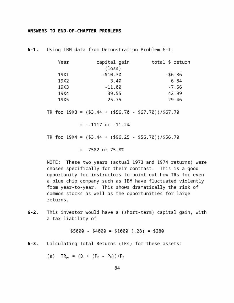
MAJOR CHAPTER HEADINGS [Contents]
Dealing With Uncertainty
Using Probability Distributions
Calculating Expected Return[expected value/expected return]
Calculating Risk[standard deviation using probabilities]
Portfolio Return And Risk
Portfolio Expected Return[portfolio weights; portfolio expected return is a weighted average of individual security returns]
Portfolio Risk[portfolio risk is not a weighted average]
Analyzing Portfolio Risk
Risk Reduction: The Insurance Principle[insurance principle—risk sources are independent]
Diversification[random diversification; international diversification; how many securities are needed to diversify properly?]
Markowitz Diversification[basic ideas of Markowitz]
Measuring Comovements In Security Returns
Markowitz Portfolio Theory[description; the basic concepts]
The Correlation Coefficient[description; graphs of perfect positive correlation, perfect negative correlation, 0.55 positive correlation]
Covariance[description; relation with correlation coefficient]
97
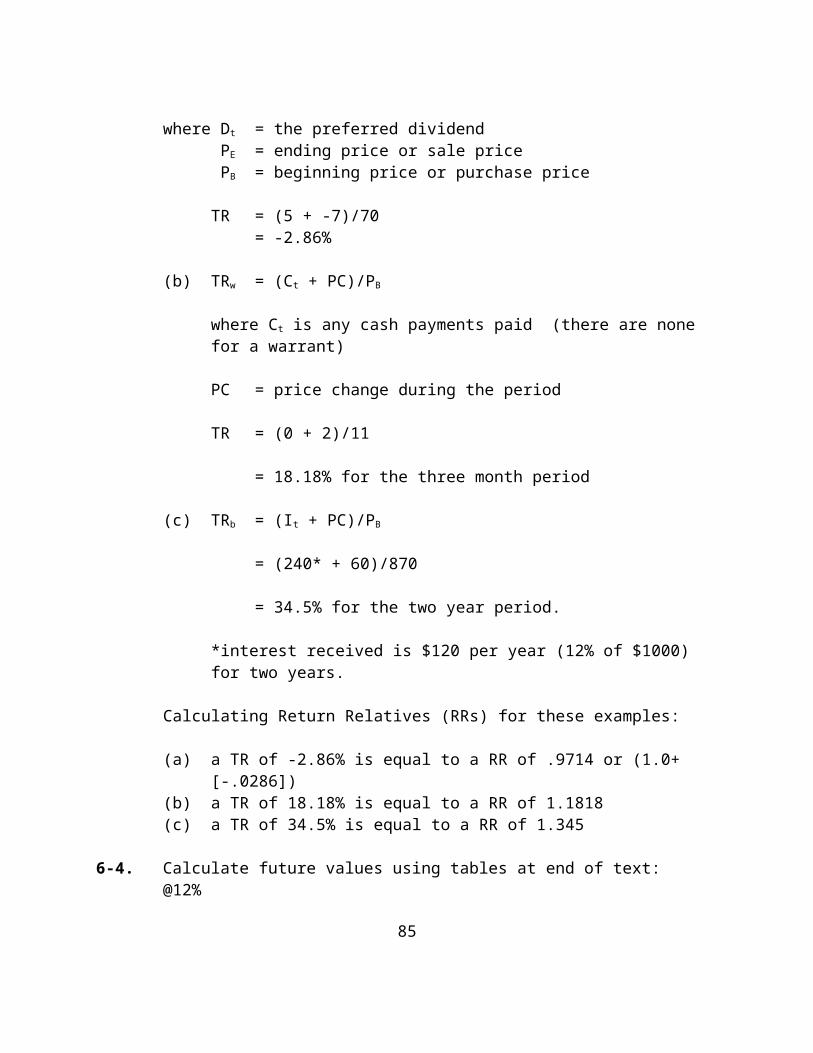
Calculating Portfolio Risk
The Two-Security Case[detailed example and explanation]
The n-Security Case[formula; explanation; the variance-covariance matrix illustrated]
Simplifying the Markowtiz Analysis[the problem with too many covariances]
Efficient Portfolios
[the attainable set and the efficient set of portfolios]
Diversifiable Risk Versus Nondiversifiable Risk
[the concepts of systematic and nonsystematic risk—what diversification can accomplish]
The Capital Asset Pricing Model
[the concept of beta; graphs of beta]
The CAPM’s Expected Reeturn-Beta Relationship[the CAPM model; the SML]
POINTS TO NOTE ABOUT CHAPTER 7
Tables and Figures
NOTE: The figures and tables in this chapter are either the standard figures typically seen in portfolio theory or illustrate calculations and examples. As such, they can be referred to directly or instructors can substitute their own figures and examples without any loss of continuity.
98
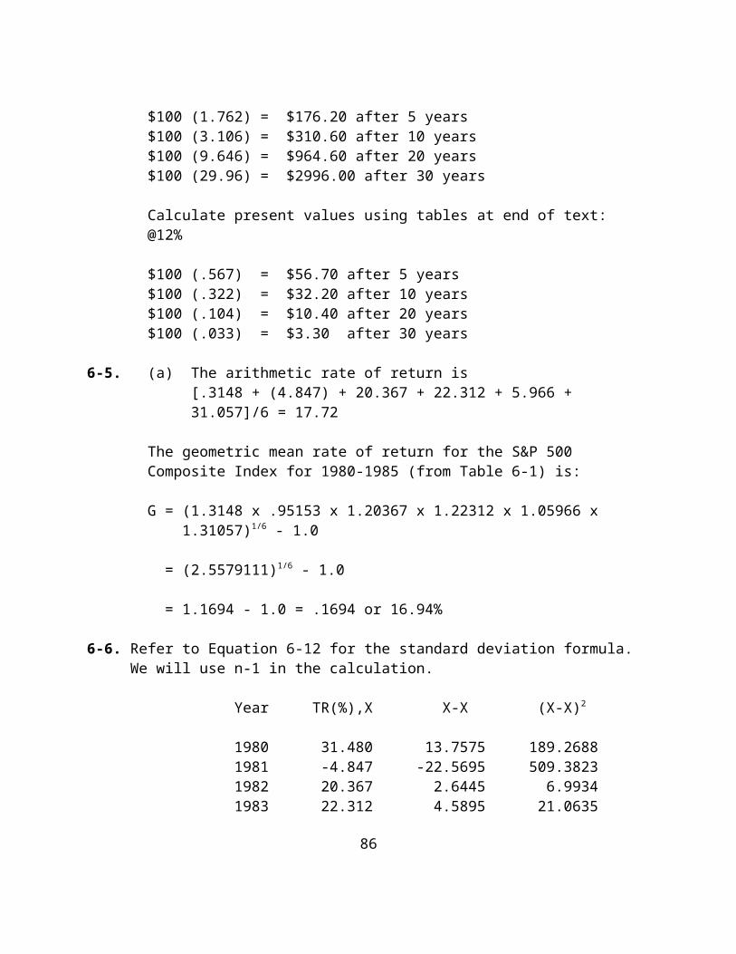
Table 7-1 illustrates the calculation of standard deviation when probabilities are involved.
Table 7-2 shows the expected standard deviation of annual portfolio returns for various numbers of stocks in a portfolio.
Table 7-3 illustrates the variance-covariance matrix involved in calculating the standard deviation of a portfolio of two securities and of four securities. The point illustrated is that the number of covariances involved increases quickly as more securities are considered.
Figure 7-1 illustrates a discrete and a continuous probability distribution.
Figure 7-2 illustrates the concept of risk reduction when returns are independent. Risk continues to decline as the number of observations increase.
Figure 7-3 illustrates diversification possibilities with international stocks as opposed to only domestic stocks.
Figures 7-4, 7-5 and 7-6 illustrate, respectively:
. the case of perfect positive correlation, . the case of perfect negative correlation,
. the case of partial positive correlations between the returns for two securities based on the average correlation for NYSE stocks of approximately +0.55.
Figure 7-7 illustrates the effects of portfolio weights on the standard deviation of the portfolio.
Figure 7-8 shows the attainable set and the efficient set of portfolios as developed by Markowitz. This allows students to understand the efficient frontier.
Figure 7-9 illustrates the important concepts of systematic (non-diversifiable) risk and nonsystematic (diversifiable) risk. These terms are used throughout the course.
Figure 7-10 is a graph of different betas.
Figure 7-11 shows the SML, which is the CAPM in graphical form.
99
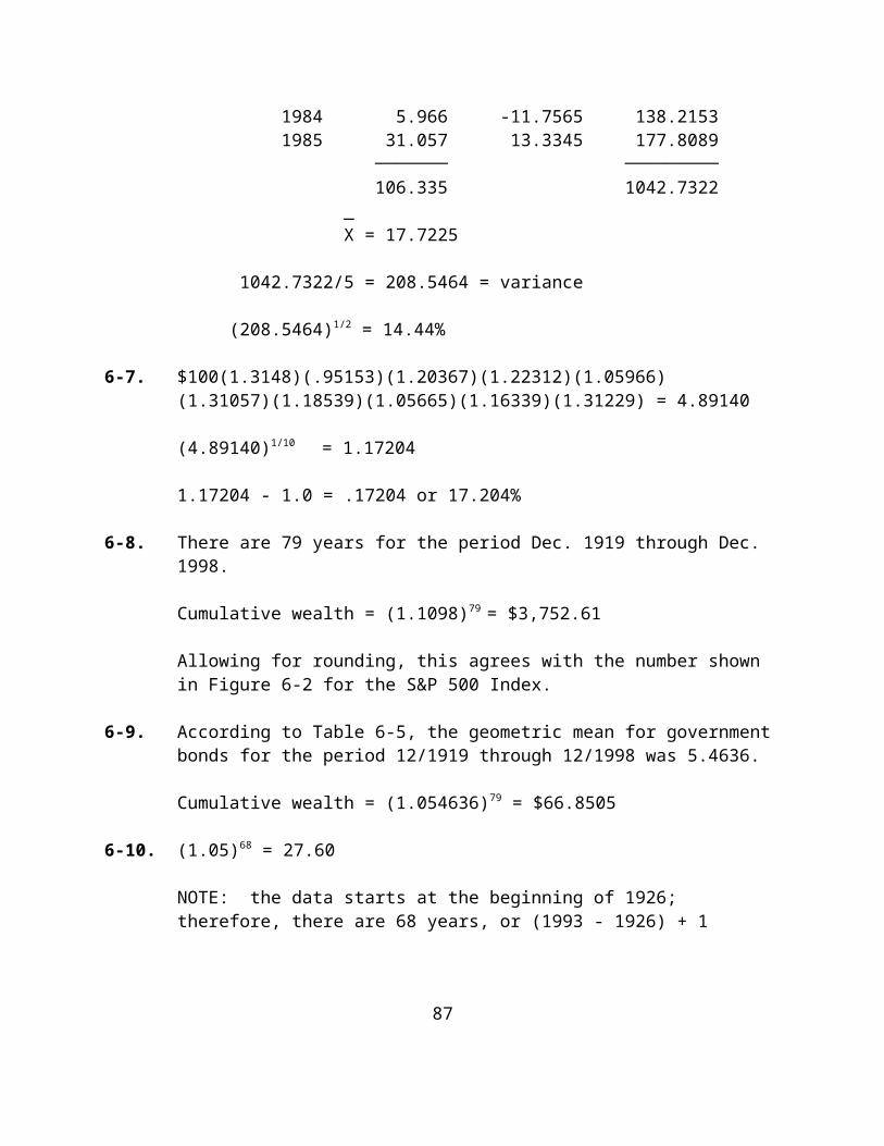
Box Inserts
There are no boxed inserts for Chapter 7.
100
ANSWERS TO END-OF-CHAPTER QUESTIONS
7-1. Historical returns are realized returns, such as those reported by Ibbotson Associates and Wilson and Jones in Chapter 6.
Expected returns are ex ante returns--they are the most likely returns for the future, although they may not actually be realized because of risk.
7-2. The expected return for one security is determined from a probability distribution consisting of the likely outcomes, and their associated probabilities, for the security.
The expected return for a portfolio is calculated as a weighted average of the individual securities’ expected returns. The weights used are the percentages of total investable funds invested in each security.
7-3. The basis of portfolio theory is that the whole is not equal to the sum of its parts, at least with respect to risk. Portfolio risk, as measured by the standard deviation, is not equal to the weighted sum of the individual security standard deviations. The reason, of course, is that the covariances must be accounted for.
7-4. In the Markowitz model, three factors determine portfolio risk: individual variances, the covariances between securities, and the weights (percentage of investable funds) given to each security.
7-5. The Markowitz approach is built around return and risk. The return is, in effect, the mean of the probability distributions, and variance is a proxy for risk. Efficient portfolios, a key concept, are defined on the basis of return and risk--that is, mean and variance.
7-6. A stock with a large risk (standard deviation) could be desirable if it has high negative correlation with other stocks. This will lead to large negative covariances which help to reduce the portfolio risk.
101
7-7. The correlation coefficient is a relative measure of risk ranging from -1 to +1. The covariance is an absolute measure of risk.
Since COVAB = rAB A B
COVAB
rAB = ───── A B
7-8. Markowitz was the first to formally develop the concept of portfolio diversification. He showed quantitatively why, and how, portfolio diversification works to reduce the risk of a portfolio to an investor. In effect, he showed that diversification involves the relationships among securities.
7-9. The expected return for a portfolio of 500 securities is calculated exactly as the expected return for a portfolio of 2 securities--namely, as a weighted average of the individual security returns. With 500 securities, the weights for each of the securities would be very small.
7-10. Each security in a portfolio, in terms of dollar amounts invested, is a percentage of the total dollar amount invested in the portfolio. This percentage is a weight, and the general assumption is that these weights sum to 1.0, accounting for all of the portfolio funds.
7-11. The expected return for a portfolio must be between the lowest expected return for a security in the portfolio and the highest expected return for a security in the portfolio. The exact position depends upon the weights of each of the securities.
7-12. Naive or random diversification refers to the act of randomly diversifying without regard to relevant investment characteristics such as expected return and industry classification.
7-13. For 10 securities, there would be n (n-1) covariances, or 90. Divide by 2 to obtain unique covariances; that is, [n(n-1)] / 2, or in this case, 45.
7-14. With 30 securities, there would be 900 terms in the variance-covariance matrix. Of these 900 terms, 30 would
102
be variances, and n (n - 1), or 870, would be covariances. Of the 870 covariances, 435 are unique.
7-15. Most stocks have a significant level of co-movement with
the overall market of stocks--that is, they have systematic risk. The risks are not independent, and risk cannot be eliminated because common sources of risk affect all firms.
7-16. The correlation coefficient is more useful in explaining diversification concepts because it is a relative measure of association between security returns--we know the boundaries of the association.
7-17. Investors should expect stock and bond returns to be positively related, and bond and bill returns, and these relationships have been true in the past. Stocks and gold have been negatively related, but stocks and real estate have been positively related.
7-18. The number of unique covariances needed for 500 securities using the Markowitz model is:
n(n-1) 500(499) 249,500 ────── = ──────── = ─────── = 124,750 2 2 2
The total pieces of information needed:
[n(n+3)]/2 = [500(503)]/2 = 251,500
CFA7-19. c
CFA7-20. c
CFA7-21. d
CFA7-22. d
CFA7-23. b
103

7-24. No—their systematic risk differs, and they should priced in relation to their systematic risk
7-25. c
7-26. d answer b: exp. return is always a wgtd.av.)
7-27. c (30 securities would have 30 x 30 = 900 terms)
7-28. a,b, and d
7-29. b
104
ANSWERS TO END-OF-CHAPTER PROBLEMS
7-1. (.15)(.20) = .030(.20)(.16) = .032(.40)(.12) = .048(.10)(.05) = .005(.15)(-.05) = -.0075 .1075 or 10.75% = expected return
To calculate the standard deviation for General Foods, use the formula
n VARi = [PRi-ERi]2Pi
i=1
VARGF = [(.20-.1075)2.15] + [(.16-.1075)2.20] + [(.12-.1075)2.40] + [(.05-.1075)2.10] + [(-.05-.1075)2.15]
= .00128 + .00055 + .00006 + .00033 + .00372 = .00594
Since i = (VAR)1/2
the for GF = (.00594)1/2 = .0771 = 7.71%
7-2. (a)
(.25)(15)+(.25)(12)+(.25)(30)+(.25)(22)= 19.75%
(b)(.10)(15)+(.30)(12)+(.30)(30)+(.30)(22)= 20.70%
(c)(.10)(15)+(.10)(12)+(.40)(30)+(.40)(22)= 23.50%
7-3. (a) (1){3 decimal places} (1/3)2(10)2 = 11.089 +(1/3)2( 8)2 = 7.097 +(1/3)2(20)2 = 44.360 + (2)(1/3)(1/3)(.6)( 8)(10) = 10.645 + (2)(1/3)(1/3)(.2)(20)(10) = 8.871 + (2)(1/3)(1/3)(-1)(20)( 8) = -35.485
46.577 variance = 46.577; = 6.82%
100
101
(2) variance = (.5)2(8)2 + (.5)2(20)2 + 2(.5)(.5) (-1)(20)(8) = 16 + 100 - 80 = 36 = 6%
(3) variance = (.5)2(8)2 + (.5)2(16)2 + 2(.5)(.5)(.3)(8)(16) = 16 + 64 + 19.2 = 99.2 = 9.96%
(4) variance = (.5)2(20)2 + (.5)2(16)2 + 2(.5)(.5)(8)(20)(16) = 100 + 64 + 128 = 292 = 17.09%
(b)(1) variance = (.4)2(8)2 + (.6)2(20)2 + 2(.6)(.4) (-1)(8)(20) = 100 + 144 - 76.8 = 77.44 = 8.8%
(2) variance = (.6)2(8)2 + (.4)2(20)2 + 2(.6)(.4) (-1)(8)(20) = 23.04 + 64 - 76.8 = 10.24 = 3.2%
(c) In part (a), the minimum risk portfolio is 50% of the portfolio in B and 50% in C. But this may not be the highest return. For the combinations in (a) above, the return/risk combinations are:
Portfolio ER SD
(1) A, B, C 19% 6.82%(2) B&C 21% 6.00%(3) B&D 17% 9.96%(4) C&D 26% 17.09%
Combination (BC) is clearly preferable over (ABC) and (BD), because there is a higher ER at lower
102
risk. The choice between (BC) and (CD) would depend on the investor's risk-return tradeoff.
NOTE: Problems 7-4 through 7-7 are based on the same data.
7-4. We will confirm the expected return for the third case shown in the table-- 0.6 weight on EG&G and 0.4 weight on GF. Each of the other expected returns in column 1 are calculated exactly the same way.
ERp = 0.6 (25) + 0.4 (23) = 24.2
7-5. We will confirm the portfolio variance for the third case, 0.6 weight on EG&G and 0.4 weight on GF. Each of the other portfolio variances in column 2 are calculated exactly the same way.
variancep = (.6)2(30)2 + (.4)2(25)2 + 2(.6)(.4)(112.5)
= 324 + 100 + 54 = 478
7-6. Knowing the variance for any combination of portfolio weights, the standard deviation is, of course, simply the square root. Thus, for the case of 0.6 and 0.4 weights, respectively, using the variance calculated in 7-5, we confirm the standard deviation as
(478)1/2 = 21.86 or 21.9 as per column 3.
7-7. The lowest risk portfolio would consist of 20% in EG&G and 80% in GF.
CFA7-8. d
CFA7-9. c
CFA7-10. b
CFA
103
7-11. a
CFA7-12. b
7-13. (a) In order to calculate the beta for each stock, it is necessary to calculate each of the covariances with the market, using the correlation coefficient for the stock with the market, the standard deviation of the stock, and the standard deviation of the market.
Stock A cov = (.8)(25)(21) = 420
beta = 420/(20)2 = 0.952
Stock B cov = (.6)(30)(21) = 378
beta = 378/(21)2 = 0.857
(b) From the SML, Ri = 8 + (12-8)bi
Stock A = 8 + (12-8)(0.952) = 11.8% Stock B = 8 + (12-8)(0.857) = 11.4%
7-14. (a) ER = (.6)(7) + (.4)(12) = 9% SD = .4(20) = 8%
(b) ER = (-.5)(7) + (1.5)(12) = 14.5% SD = 1.5(20)= 30%
(c) ER = (0)(7) + (1.0)(12) = 12% SD = 20%
7-15. E(Ri) = 7.0 + (13.0-7.0)bi = 7.0 + 6.0bi
GF 7 + 6( .8) = 11.8% < 12% undervaluedPepsiCo 7 + 6( .9) = 12.4% < 13% undervaluedIBM 7 + 6(1.0) = 13.0% < 14% undervaluedNCNB 7 + 6(1.2) = 14.2% > 11% overvaluedEG&G 7 + 6(1.2) = 14.2% < 20% undervaluedEAL 7 + 6(1.5) = 16.0% > 10% overvalued
104

7-16. If Exxon is in equilibrium, the relationship is:
.14 = RF + [E(RM) - RF] ß
= 6 + [E(RM) - 6] 1.1
Therefore,
a. the slope of the SML must be [E(RM) - 6] or approximately 7.3% in order for the relationship to hold on both sides
b. the expected return on the market is 7.3% + 6% or 13.3%(approximately)
CFA7-17. d
105
Chapter 8: Bond Yields and Prices
CHAPTER OVERVIEW
Chapter 8 concentrates on the issues of bond yields and prices. In effect, virtually all of the calculations concerning bonds are contained in this chapter, thereby allowing Chapter 9 to concentrate on analysis and management issues.
The first part of Chapter 8 deals with bond yields and begins with a discussion of interest rates because of their obvious relationship to bond yields. After briefly considering terminology, the chapter discusses what determines interest rates. Important concepts such as the real rate of interest and the Fisher hypothesis are considered here.
The important concept of yield to maturity is examined in detail. Both conventional bonds and zero-coupon bonds are considered. The issue of the effect of reinvestment rates on realized returns is explained in detail. Yield-to-call and horizon return are also discussed.
The next part of the chapter focuses on bond prices by explaining the capitalization of income method of valuation and then applying this methodology to the valuation of bonds. Detailed examples are provided based on semiannual discounting.
Next, bond price changes are considered in detail. This starts with bond price changes over time (price must converge to face value at maturity) and then considers bond price changes as a result of interest rate changes (Malkiel's Theorems).
A central part of this discussion is the measurement of bond price volatility, centering on duration. This key variable is defined and described, and all of the relationships involving duration are illustrated. Convexity is also briefly discussed.
Instructors may wish to add to the material in this chapter, or expand on various issues such as bond valuation, yield to maturity, and horizon return analysis. The essential building blocks are presented here, and additional work is possible
106

depending upon preferences and time constraints. This is the minimum material that students should be exposed to, but it is also a very reasonable package in terms of what beginners should be expected to master. It allows total flexibility for
instructors to add to this material with their own examples, problems, calculations, and so forth.
CHAPTER OBJECTIVES
To consider the determination of market interest rates as a natural complement to the discussion of bond yields.
To analyze important calculations such as yield to maturity, yield to call, and realized compound yield.
To explain the concept of valuation (capitalization of income) and apply it specifically to bonds.
To analyze the issues involved with both prices and yields, with particular emphasis on calculations.
107
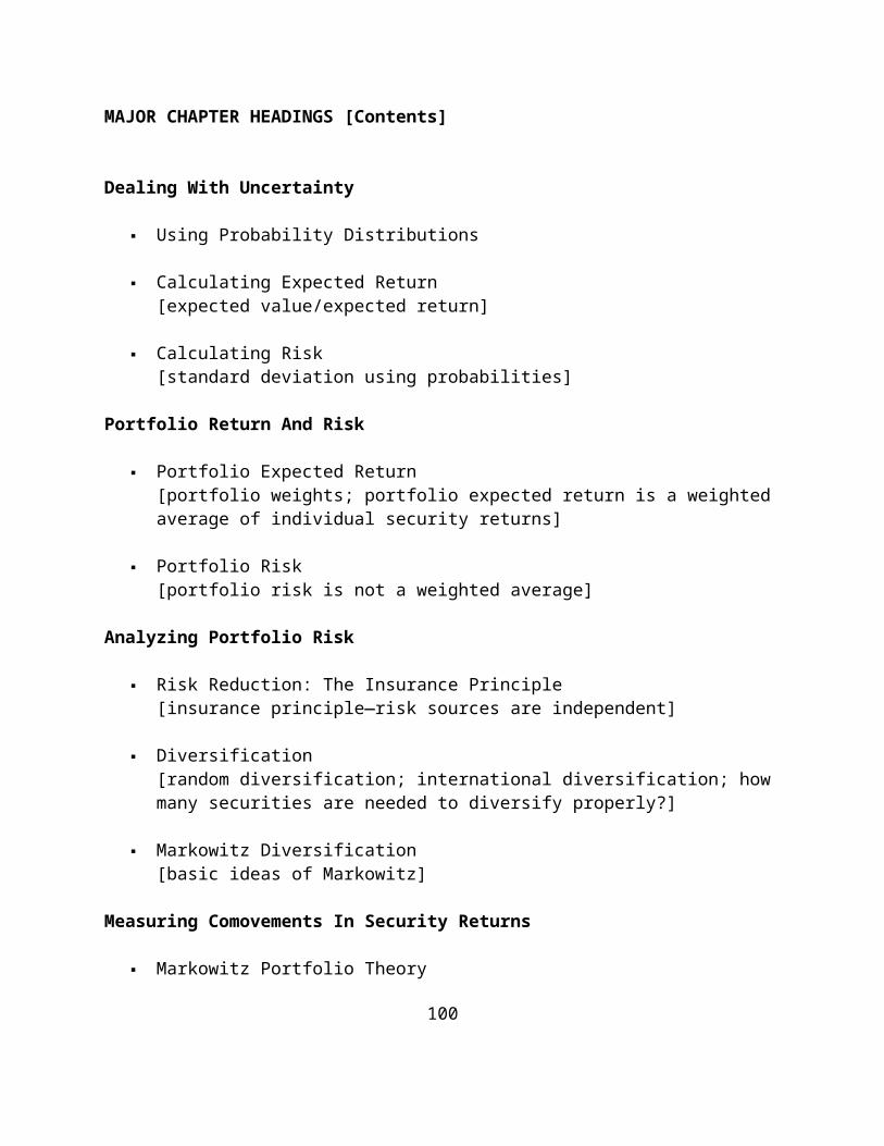
MAJOR CHAPTER HEADINGS [Contents]
Bond Yields
[bond yields and interest rates are the same concept]
The Basic Components of Interest Rates[real rate of interest; Fisher hypothesis]
Measuring Bond Yields[current yield; yield to maturity; yield to call; realized compound yield; reinvestment risk; interest-on-interest; calculations; examples for both coupon bonds and zero-coupon bonds; horizon return]
Bond Prices
The Valuation Principle[the calculation of intrinsic value using discounted cash flow analysis]
Bond Valuation[calculating bond prices using semiannual discounting; required yield]
Bond Price Changes
Bond Price Changes Over Time[price must converge to face value by maturity date]
Bond Price Changes As a Result of Interest Rate Changes[explanations and illustrations of Malkiel’s bond theorems; the implications of Malkiel’s theorems to investors--coupon and maturity are key factors, given a change in rates]
Measuring Bond Price Volatility: Duration[definition; calculation; understanding duration; measuring price changes using duration; examples of all calculations; convexity explanation, with diagram; some conclusions on duration]
108
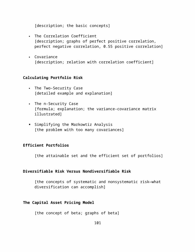
Appendix 8-A Convertible Bonds
POINTS TO NOTE ABOUT CHAPTER 8
Tables and Figures
Table 8-1 illustrates the calculation of realized yield based on varying reinvestment rates. This analysis is useful to emphasize in order for students to really understand interest-on-interest and related concepts such as the yield to maturity and the realized compound yield.
Table 8-2 is of interest in showing bond price calculations. It illustrates the inverse relationship between prices and yields for varying time periods.
Table 8-3 is an example of calculating the duration of a bond.
Figure 8-1 is a simple illustration of the fact that bond prices must converge by maturity date to the face value. Thus, other things equal, a discount bond must rise in price while a premium bond must decline in price, both moving to $1,000 by maturity date.
Figure 8-2 illustrates the convex relationship between yields and prices. Instructors may choose to explain this concept in a basic manner in a beginning course, but it probably is not necessary, or desirable, to elaborate on it in too much detail.
Figure 8-3 illustrates the cash flow pattern of a coupon-paying bond as an aid in understanding the difference between a bond's maturity and its duration.
Figure 8-4 illustrates the convex relationship between yields and prices as an aid in understanding the convexity principle.
109

Box Inserts
Box 8-1 illustrates how duration is used to manage actual bond portfolios. It defines duration, explains how investors can use it, and shows how some particular mutual fund managers actually do use it in managing their bond portfolios.
110

ANSWERS TO END-OF-CHAPTER QUESTIONS
8-1. Yield to maturity (YTM) is defined as the indicated (promised) compounded rate of return an investor will receive from a bond purchased at the current market price and held to maturity.
Two methods of determining YTM are:*
(a) bond tables(b) solving the equation for YTM using a calculator or
software
*We ignore the approximation formula because there is little or no justification for using it in today's world of computers and calculators.
8-2. It is YTM that equilibrates in the marketplace, and bond prices change to reflect this equilibration. Investors invest on the basis of promised yields (i.e., YTMs), reflecting current conditions in the marketplace. Bond prices must adjust to these new conditions as reflected in new YTMs.
8-3. To say that YTM is an expected yield is to say that if we purchase the bond today at its current market price and hold it to maturity (and the issuer does not default), and if we reinvest the coupons at the indicated YTM rate, we can expect to earn the stated YTM. Obviously, the rate is promised--it may not materialize. If the conditions outlined do not occur, the actual yield will differ from the expected yield.
8-4. Investors buy bonds, like any other asset, on the basis of their expected future performance. Therefore, they must consider measures of the promised return. We use the realized compound yield to calculate what we actually earned, but we must make estimates of what we expect to earn when we purchase an asset.
8-5. Interest on interest refers to the fact that investment in a bond generates coupon (interest) income which in turn is reinvested to earn additional interest. Therefore, we are earning interest on interest already
111
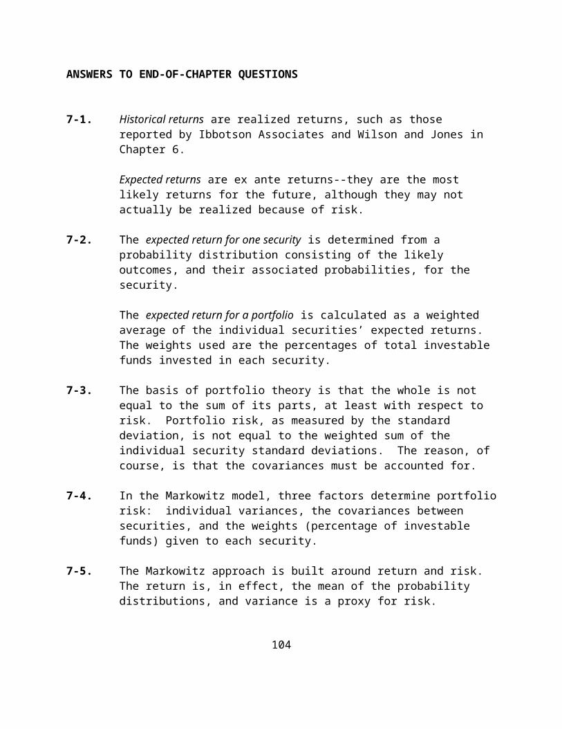
earned. It is part of the compounding process inherent in the nature of bond calculations.
8-6. Bond A will be more affected because of the higher coupon.
8-7. Promised yield (YTM) is exactly that--what an investor expects to earn over the life of a bond purchased at the current price and held to maturity. However, this depends upon the rates at which the coupons are assumed to be reinvested over time.
Realized yield indicates what has been earned on a bond held to maturity, given a constant reinvestment rate.
Typically, because of reinvestment rate risk (interest-on-interest), the realized (actual) yield will differ from the promised yield.
8-8. One way to eliminate reinvestment rate risk is with zero coupon bonds. Since there are no coupons to reinvest, there is no reinvestment rate risk. Investors know their realized yields at time of purchase if the bond is held to maturity (and, of course, barring default).
8-9. The intrinsic value of any asset is usually thought of as a present value process--the present value of the expected cash flows from that asset. These cash flows must be discounted at an appropriate discount rate; therefore, intrinsic value and present value are closely related.
8-10. The price of a bond is determined as the present value of its coupons and the principal repayment (ignoring zero coupon bonds). The discount rate used is the appropriate market yield for that issue. The present value process for a standard bond will involve use of both a present value term (for the principal repayment) and a present value of the annuity term (for the coupons).
This process is relatively straightforward because the payment dates and the amounts of coupon and principal repayment are known at time of issuance. Furthermore, it is relatively easy to determine the discount rate from current market rates on similar bonds.
112
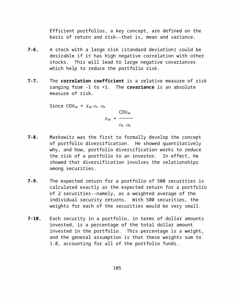
8-11. The simple point here is that there is obviously a difference between using annual and semiannual discounting. The exact effects of the difference are somewhat complex.
• In general, if the discount rate used in the valuation is higher than the coupon rate, annual discounting will result in a higher present value than will semiannual discounting (a result of a higher present value for the principal repayment when using annual discounting).
• On the other hand, if the discount rate is less than the coupon rate, semiannual discounting produces the higher present value (a result of a higher present value for the coupons when using semiannual discounting).
Based on the above, we would predict that a 10%, 8 year bond, given a discount rate of 12%, would have a higher value using annual discounting as opposed to semiannual discounting. Specifically,
Annual discounting Semiannual discounting $100 (4.9676) = $496.76 $50 (10.1059) = $505.30 $1000 (.4039) = $403.90 $1000 (.3936) = $393.60 $900.66 $898.90
8-12. The implications of Malkiel’s bond price theorems to bond investors concern how investors should act with regard to trading in bonds. Specifically, the two bond variables of major importance in assessing price changes are:
• the coupon and • the maturity.
To receive the maximum impact from an expected change in interest rates, investors should purchase low coupon, long-maturity bonds.
8-13. Duration accounts for the entire pattern (both size and timing) of a bond's cash flows over its life. It tells investors (in years) the economic lifetime of a bond,
113
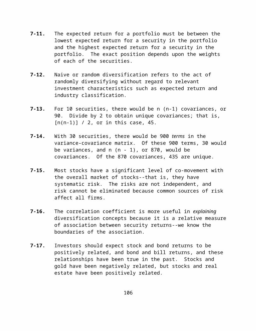
whereas time to maturity focuses only on the return of principal at the maturity date.
8-14. • Duration increases with time to maturity, but at a decreasing rate, particularly beyond 15 years time to maturity.
• The coupon is inversely related to duration.
For a zero coupon bond, duration is equal to time to maturity.
8-15. This investor should choose bonds with the longest duration. Duration is positively related to maturity and negatively related to coupon. Since duration is additive, a portfolio's duration is a weighted average of each individual bond's duration.
8-16. Duration may not be a complete measure of bond risk. It measures volatility, which is only one aspect of the risk in bonds. It may or may not be the best measure, depending on the investor's perspective. If volatility is the most important factor to an investor, duration is probably the best measure to use.
8-17. If the coupon rate is below the current required yield, a bond is selling for a discount; if the coupon rate is above, it is selling for a premium.
8-18. The investor makes an assumption about the reinvestment rate expected to prevail over the planned investment horizon. The investor may also make an assumption about the yield to maturity expected to prevail at the end of the planned investment horizon, which in turn is used to estimate the price of the bond at that time.
8-19. For all coupon-paying bonds, duration is always less than time to maturity. Duration expands with time to maturity, but at a decreasing rate, particularly as we get beyond 15 years. For a zero coupon bond, duration is equal to time to maturity.
Both coupon and yield to maturity are inversely related to duration.
114

8-20. Convexity is the term used to refer to the degree to which duration changes as the yield to maturity changes. As the change in yield increases, the error that results from using a straight line to estimate a bond's price behavior as given by a curve increases.
Bond investors can use convexity calculations to improve the estimate of total percentage price change referred to in the duration discussion. Although still an approximation, this estimate is improved over that using only duration.
115

ANSWERS TO END-OF-CHAPTER PROBLEMS
8-1. 1.
Future date Assumption A Assumption B 6 months $50/(1.04) = 48.077 1 year $100/(1.08) = 92.593 50/(1.04)2 = 46.228 1.5 years 50/(1.04)3 = 44.450 2 years $100/(1.08)2 = 85.734 50/(1.04)4 = 42.740 2.5 years 50/(1.04)5 = 41.096 3 years $100/(1.08)3 = 79.383 50/(1.04)6 = 39.516 3 years $1000/(1.08)3 = 793.832 1000/(1.04)6 = 790.315 $1051.54 $1052.42
2. Under either assumption A or B, price = $1000 (par).
Using a calculator, the discount factors can be determined by raising the rates to the appropriate power and taking the reciprocal.
8-2. Assumption A Assumption B
100 1 1000 50 1 1000P = ───[1- ───────] + ────── P = ───[1- ────── ] + ───── .08 (1.08)3 (1.08)3 .04 (1.04)6 (1.04)6
P = 1250[.2062] + 793.83 P = 1250[.2097] + 790.31
P = 257.75 + 793.83 = $1051.58 P = 262.13 + 790.31
= $1052.44
8-3. 25 1 1000 P = ─── [1 - ──────── ] + ──────── .02 (1.02)12 (1.02)12
P = 1250[.2115068] + 788.4932
P = 264.38353 + 788.4932 = $1052.88
8-4. Given the amount of the coupon and the market interest rate, semiannual coupon payments provide a higher price for securities selling at a premium, but a lower price
120

for those securities selling at a discount. In this problem the coupon rate is 10% and the market rate 12%; therefore, the security will be selling at a discount, and we should expect the price for semi-annual payments to be less than the price using annual payments.
Annual discounting: $100 X 4.968 = $496.80 $1000 X .404 = $404.00 ─────── $900.80
Semiannual discounting: $50 X 10.106 = $505.30 $1000 X .394 = $394.00 ─────── $899.30
For the sake of comparison, the alternative methodology suggested in Demonstration Problem 8-2 is applied here, and with more decimal places. One can compare the answers to see how close they are.
--------------ANNUAL--------------
100 1 1000P = ────[1 - ─────── ] + ─────── .12 (1.12)8 (1.12)8
P = 833.333[.5961168] + 403.883
P = 496.764 + 403.883 = $900.647
-----------SEMIANNUAL-------------
50 1 1000P = ───[1 - ──────── ] + ──────── .06 (1.06)16 (1.06)16
P = 833.333[.6063537] + 393.6463
P = 505.29474 + 393.6463 = $898.941
8-5. Solve for price for the 10% coupon bond in Problem 8-4: r = 12%: Use the tables at the end of the text.
121

$50 X 15.046 = $752.30 [15.046 = PV annuity @ 40 periods,6%]
$1000 X .097 = $ 97.00 ─────── $849.30
According to Malkiel’s principles, for a given change in market yields, changes in bond prices are directly related to time to maturity.
8-6. 30 $50 $1000P = ─────── + ──────── = $862.34
t=1 (1.06)t (1.06)30
or
P = $50(13.7648) + $1000(.1741)
= $688.24 + 174.10
= $862.34
8-7. r = [FV/P]1/2n - 1 for a zero-coupon bond
For a zero-coupon bond sold at $400,
= [$1000/$400]1/20 - 1= 2.5.05 - 1= 1.04688 - 1= .04688 or 4.688% semiannually or 9.376% annually
For a zero-coupon bond sold at $300
= 3.333.05 - 1= 1.06204 - 1= .06204 or 6.204% semiannually or 12.408% annually
8-8. realized compound yield = [total future dollars/purchase price of bond]1/2n – 1.0
122
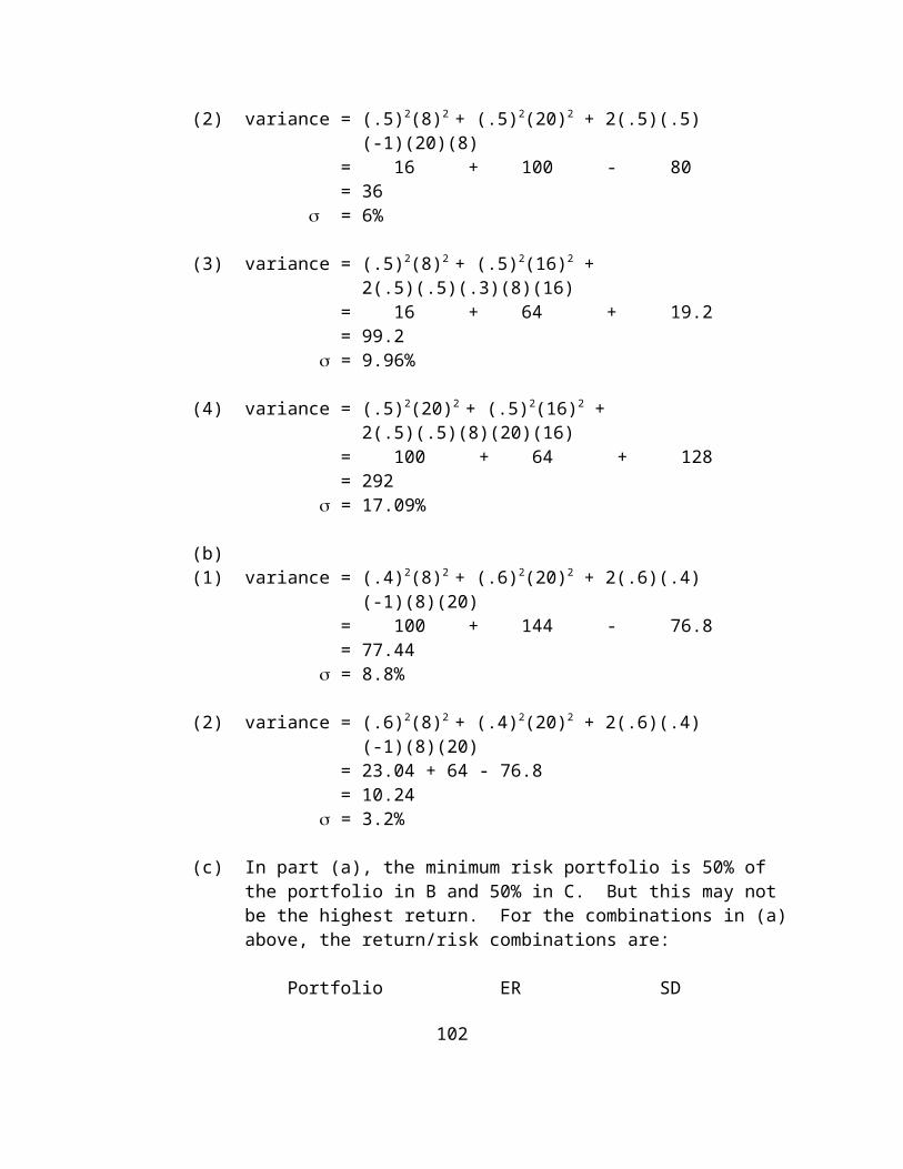
= [$5751/$1000]1/40 - 1.0= [5.751].025 - 1.0= .0447 or 4.47% semiannually or 8.94% annually
NOTE: This problem is based on Table 8-1 and:
• total future dollars = total return in $ + purchase price
• purchase price = $1000• total return = sum of an annuity for 40 periods, 8%
reinvestment, $50 semiannual coupons or95.026 [$50] = $4751 where 95.026 is the sum of the annuity factor for 40 periods, 4%
8-9. Given: 12%, 10-year bond bought at par, reinvestment rate = 10%
(a) total return = sum of an annuity [20 periods, 5%] X $60
= 33.066 X $60 = $1983.96
(b) interest-on-interest = amount attributable to reinvestment = total return - coupon income
= $1983.96 - $1200 = $783.96
(c) realized return = [total future dollars/purchase
price]1/2n - 1.0 price]1/2n – 1.0
= [$2983.96/$1000].05 - 1.0 = 2.98396.05 - 1.0 = .05618 or 5.618%
semiannually or 11.237% annually
NOTE: total future dollars = total return + purchase price = $1983.96 + $1000 = $2983.96
8-10. @ 15% required rate of return, price = $811.08
123
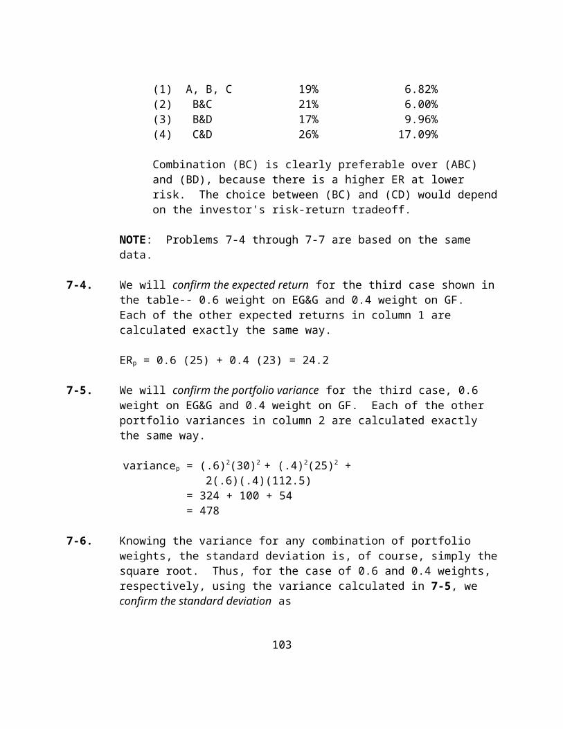
@ 17% required rate of return, price = $717.14@ 20% required rate of return, price = $608.84
8-11. The duration is calculated as 6.16 years. Dividing by 1+YTM, or 1.1361, the modified duration is calculated as 5.42.
8-12. Using a price of $300, the YTM is 17.07%. This problem is easily solved with a calculator.
8-13. Start with 15 years. The duration is 8.84 years. Using 20 years, the duration is 9.07 years. At 25 years, the duration has decreased to 8.82 years.
8-14. To calculate the yield to first call (YTC):
Market Price = $970$100 is the annual dollar coupon; $50 semiannual10 is the number of years to maturityBUT 5 is the number of years until first call, And this is used in the calculation$1050 is the call price, as given in the problem; use this number instead of $1,000 as the future value
The YTC is 11.57% and the YTM is 10.49%. The YTC is greater than the YTM because of the call premium received when the bond is called.
8-15. using semiannual interest rates
(a) 12.3394%(b) 8.4632%(c) 15.3231%
8-16. • recognize that the dollar coupon is $100• use the correct price of $1093.75 or 109.375% of par
• there are 28 periods on a semiannual basis
Current Yield = 9.14%
YTM = 8.8209%
124
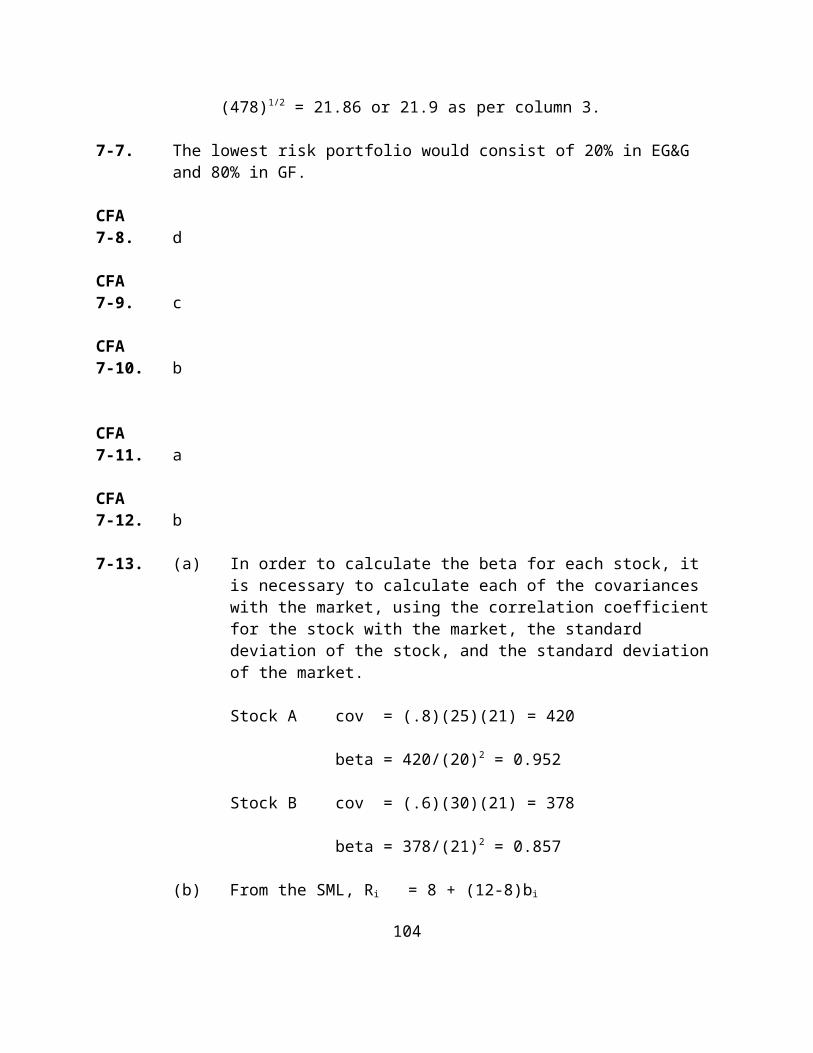
8-17. Doubling the maturity to 28 years changes the YTM to 9.0721%.
The current yield does not change.
8-18. The current market price is $899.47.
With a YTM of 11.5% instead of 12.5%, the price of the bonds would be $964.65. If the market is demanding a lower rate on the bonds, the market price would be higher. In other words, the discount rate is lower, therefore the price is higher.
8-19. The only variation here is to recognize that the current market price to be entered is $800 because it is stated that the bond is selling for 20% less than face value. The YTM is calculated as 15.21%.
8-20.
(1) (2) (3) (4) (5) (6)Future Present P.V./date Return 1/(1.04)2t value 1052.42 (1)x(5)
.5 $50 .9615385 48.076923 .0456823 .0228411.0 50 .9245562 46.227811 .0439252 .04392521.5 50 .8889964 44.449818 .0422358 .06335372.0 50 .8548042 42.74021 .0406114 .08122272.5 50 .8219271 41.096355 .0390494 .09762353.0 50 .7903145 39.515726 .0375475 .11264253.0 1000 .7903145 790.31453 .7509497 2.2528492 1.0000013 2.6744578
Duration = 2 years, 8 months, and 3 days
This bond, with a term to maturity of three years, has a duration of slightly over two years and eight months. That is, the weighted average time to the full recovery of interest and principal is two years, eight months, and three days.
8-21. The duration as calculated in Problem 8-20 is 2.67 years.
125
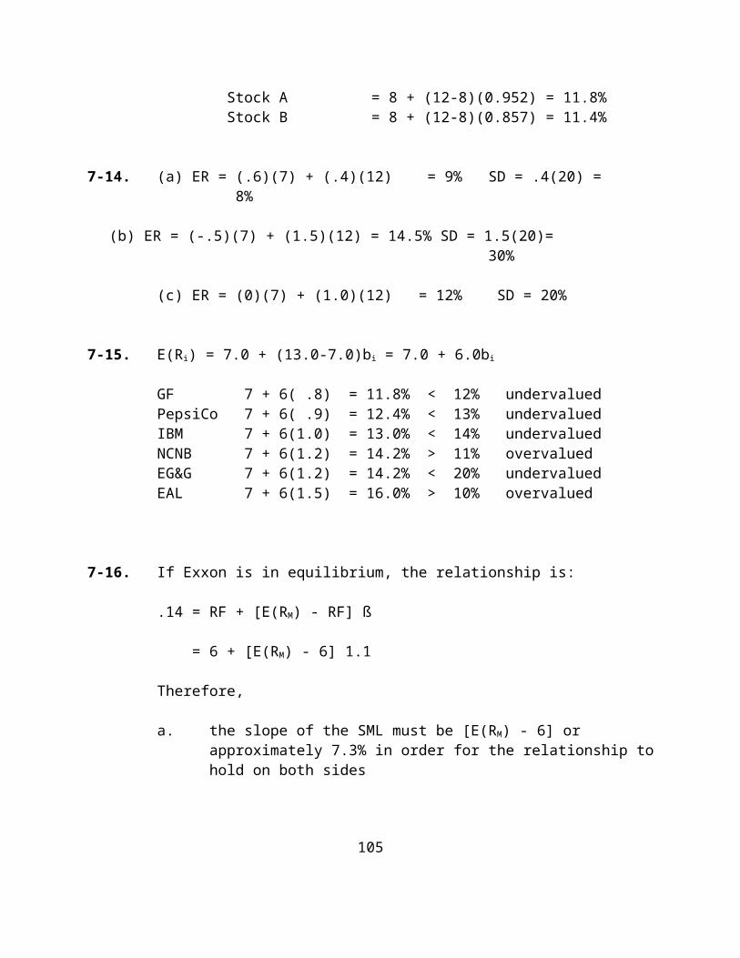
(a) modified duration = 2.67/1.04 = 2.5673.
(b) approximate price change = -2.5673 X .0050 = 1.28%. therefore, if interest rates declined to 7.5% on an annual basis, or 3.75% on a semiannual basis, the price of the bond would increase to approximately
$1,052.24 x 1.28%, or $1,065.71
Solving with a calculator for the new price of this bond, using 3.75% as the semiannual rate, produces a price of $1,066.06.
8-22. Calculate duration for a 12% coupon bond with 10 years to maturity and selling at par (i.e., the price of this bond is $1000). Use Annual Interest for this problem.
(1) (2) (3) (4) (5) (6) Year Cash flow PV factor PV of (2) PV/price (1)x(5)
1 $ 120 .8929 $107.148 .107148 .107148 2 120 .7972 95.664 .095664 .191328 3 120 .7118 85.416 .085416 .256248 4 120 .6355 76.26 .076260 .305004 5 120 .5674 68.088 .068088 .34044 6 120 .5066 60.792 .060792 .364752 7 120 .4523 54.276 .054276 .379932 8 120 .4039 48.468 .048468 .387744 9 120 .3606 43.272 .043272 .389448 10 1120 .3220 360.640 .360640 3.6064 $1000 1.000035 6.32848
Therefore, the duration is 6.33 years.
8-23. approximate % change in bond price = -D/(1+YTM) X % point change in the YTM
= -6.33/(1+.12) X (-.0075)
[NOTE: we are using annual interest here, so we divide by 1 + YTM, or 1.12.
= -5.6518 X -.0075 = +4.239%
126

Therefore, this bond would increase in price by approximately 4.24%, resulting in a price of $1,042.40.
Using a calculator, solving for the new bond price at an interest rate of 11.25% produces a price of $1,043.71.
CFA8-24. A. 1. At 8% - 10-year duration. Obviously, the
duration of a zero coupon bond is always equal to the term-to-maturity irrespective of the market rate.
2. Present value factor at 4% for 20 periods is .456; therefore issue price is $4,560.
3. Present value factor at 6% for 10 periods is .350; therefore market value a year later is $3,500. Therefore, the rate of return is:
3,500 - 4,560 -1,060───────────── = ────── = -23.25% 4,560 4,560
B. 1. Modified Duration = Duration: (1 + Market Yield/the number of coupon payments per year)
D 8 8Modified Duration = ─────── = ───────── = ──── = 7.69 years
1 + r/2 1 + .08/2 1.04
2. Percent change in bonds price = Modified Duration x
(Change In Market Yield in Basis Points)──────────────────────────────────────── 100
2007.69 x ─── = 7.69 x 2 = 15.38% 100
CFA
127
8-25. A. I. The Wiser bond’s duration is less than its maturity because some of the bond’s cash flow payments (i.e., the coupons) occur before maturity. Since duration measures the weighted average time until cash flow payment, its duration is less than its maturity. Bond duration is defined as
N PVCFt x t t = 1D = ────── N PVCFt
t = 1
II. For coupon bonds, duration is a better measure of the bond’s sensitivity to changes in interest rates. Using the bond’s maturity is deficient as a benchmark because it measures only when the final cash flow is paid and ignores all of the interim flows. Duration is a better measure because it measures the weighted average time until cash flow and thus is a more representative measure of the bond's overall cash flow sensitivity to interest rate changes. Duration takes into account coupon (inverse relationship) and yield to maturity (inverse relationship) as well as time to maturity.
B. I. Duration will increase. As rates decline, all of the cash flows increase in value, but the longest ones increase at the greatest rate. Therefore, the redemption payment has much greater effect, causing the duration to increase.
II. Duration will increase. As rates decline, all of the cash flows increase in value, but the longest ones increase at the greatest rate. Therefore, the redemption payment has much greater effect, causing the duration to increase.
128

III. Duration will decrease. The elapsing of time is accompanied by the reduction of total coupon payments and the shortening of time until the redemption payment. Therefore, because the redemption payment comes sooner, the duration decreases.
129
Chapter 9 Bonds: Analysis and Strategy
CHAPTER OVERVIEW
Valuation, prices and yields are covered in Chapter 8, and analysis and strategy in Chapter 9. The purpose of this chapter is to cover issues involving the analysis of bonds from an investor’s perspective, and some strategies that could be employed in managing a portfolio of bonds.
Chapter 9 starts with a discussion of why investors buy bonds, both domestic and foreign. Included in this discussion is a discussion of the total returns on bonds over long periods of time. Instructors should emphasize how different types of investors are interested in bonds--some for the income return and some for the chance to earn capital gains as a result of interest rate changes. The discussion of foreign bonds is a good place to once again talk about currency risks. This discussion concludes with the case for not buying bonds outlined by Peter Bernstein.
A key part of this chapter is the discussion on important considerations in managing a bond portfolio. This includes the term structure of interest rates, and the risk structure of interest rates (yield spreads). The author feels strongly that the essential elements of this material are covered while tedious details are avoided. Students in a beginning Investments course do not need to get bogged down in the details of the term structure, and the various theories to explain term structure.
The remainder of Chapter 9 is devoted to a discussion of bond strategies and management. This chapter sets the foundation for the comparable chapter on stocks (Chapter 11) by dividing the discussion of strategies into passive and active. This is consistent with modern investing approaches and also allows instructors to incorporate any discussion of Efficient Markets they may choose as well as touch on such issues as direct versus indirect investing.
130
This chapter concludes with a discussion of building a bond portfolio. The discussion is divided into how conservative investors approach this issue as opposed to aggressive investors. It concludes with a consideration of the international perspective. It is here that instructors will want to mention the use of mutual funds and closed-end funds when investing internationally.
CHAPTER OBJECTIVES
To analyze the reasons why investors buy bonds.
To recognize important considerations in managing a bond portfolio, including the term structure of interest rates and yield spreads.
To differentiate between the passive and active strategies for managing a bond portfolio.
To consider how both conservative investors and aggressive investors go about building a fixed-income portfolio.
131
MAJOR CHAPTER HEADINGS [Contents]
Why Buy Bonds?
[reasons why investors buy bonds; bond returns over long periods of time; large annual gains in bonds do occur]
Buying Foreign Bonds?
[international considerations, primarily problems in transacting; discussion of the Euro]
Important Considerations In Managing A Bond Portfolio
Understanding the Bond Market[the importance of expected inflation on the bond market; currency effects]
The Term Structure of Interest Rates[definition; yield curves; forward rates; term structure theories: expectations theory, liquidity preference theory, market preferred habitat theory, segmentation theory]
The Risk Structure of Interest Rates--Yield Spreads[definition; factors leading to yield spreads; junk bonds; yield spreads over time]
Bond Strategies
Passive Management Strategies[definition; case for doing this; buy and hold; indexing]
Immunization--A Structured Portfolio Strategy[definition; extended example]
Active Management Strategies[forecasting changes in interest rates; identifying mispricings among securities; interest rate swaps]
Building A Fixed-Income Portfolio
Conservative Investors[factors that must be considered]
Aggressive Investors[how they might behave]
The International Perspective[returns and risks; procedures]
POINTS TO NOTE ABOUT CHAPTER 9
Tables and Figures
Exhibit 9-1 is new to the 8th edition. It explains as a flow diagram, in words, what immunization is all about. This will make the discussion in Table 9-1 easier to follow.
Table 9-1 is a detailed example of the immunization principle. It is probably worth some significant class discussion in order to help students better understand duration and reinvestment rate risk (which were covered in Chapter 8).
Figure 9-1 illustrates the relationship between real GDP growth rates, CPI growth rates, and yields on 10-year Treasuries. The CPI growth rate behaves in a manner similar to bond yields.
Figure 9-2 shows yield curves for various periods, illustrating the different shapes that yield curves can take.
Figure 9-3 illustrates yield spreads for a recent period by showing differences between Baa corporates and Aaa corporates.
Box Inserts
Box 9-1 is an interesting analysis of the unusual rates on municipal bonds. The stated rates for munis exceeded those for Treasuries, and this is before the adjustment for taxes. That is, putting the muni bond yields on a taxable equivalent basis made the muni yields significantly higher. This illustrates how these relationships can fluctuate widely over time.
ANSWERS TO END OF CHAPTER QUESTIONS
9-1. Some investors are interested in bonds because they offer a steady stream of interest income over the life of the obligation and a return of principal at maturity. On the other hand, other investors are interested in bonds exactly because bond prices will change as interest rates change. Because bonds can be purchased on margin, large potential gains are possible from speculating on interest rates.
9-2. In buying and selling foreign bonds, individual investors may find it difficult to invest directly in foreign bonds both in a dollar sense and in a time sense. Secondary markets in some foreign countries are not comparable to the U. S. Treasury market. Transaction costs are an issue. Currency risk is always a potential problem.
9-3. The key factor in analyzing bonds is the behavior of interest rates. Market yields and prices for all bonds are directly related to interest rate behavior.
9-4. Two passive bond management strategies are:
(a) Buy and hold(b) Immunization--protecting a portfolio against
interest rate risk.Note, however, that immunization requires activity to succeed. It is not a true passive strategy.
9-5. Immunization is the strategy of immunizing (protecting) a portfolio against interest rate risk. It involves offsetting the two components of interest rate risk--the price risk and the reinvestment rate risk--which move in opposite directions.
Duration is the basis for immunization theory. A portfolio is immunized if its duration is made equal to a preselected investment horizon for the portfolio.
9-6. Active bond management strategies include forecasting interest rates and bond swaps. The two are related in that at least some bond swaps involve some type of forecast of interest rates (e.g., the rate anticipation swap).
9-7. A sharp decline in interest rates is, of course, the ideal environment for the bond investor seeking capital gains. Such an investor should concentrate on low coupon, long maturity bonds, or bonds with the longest duration. All bonds will perform well in such an environment, but investors may prefer certain types depending on the circumstances. For example, yield spreads should be considered. Governments can be purchased on 8-15% margin. The after-tax return of municipals may be superior. Zero coupons offer maximum volatility. And so forth.
9-8. Long maturities have greater price fluctuations; therefore, if a rise in market rates is expected, these bonds will be unattractive for speculative purposes. The lower the coupon, the higher the price volatility. Bonds selling at large discounts presumably have lower coupons. Again, these would not be preferable if rates are expected to rise.
9-9. Bond swaps--the term usually refers to the purchase and sale of bonds in an attempt to improve the rate of return on the bond portfolio by identifying temporary mispricings in the bond market. Thus, managers of bond portfolios attempt to adjust to changing conditions by identifying mispricings among securities.
9-10. Horizon analysis is one form of interest rate forecasting. It involves the projection of bond performance over a planned investment horizon. The investor evaluates bonds being considered for purchase over a selected holding period in order to determine which will perform the best. To do this, the investor must make assumptions about reinvestment rates and future market rates and calculate the realized compound yields for the bonds being considered.
9-11. If you think the British economy will slow down, interest rates are likely to drop because of slack loan demand, and bond prices are likely to rise.
If you are bullish on the pound, you could take an unhedged position. A bearish investor might choose to hedge the position.
CFA9-12. a
CFA9-13. a
CFA9-14. c
CFA9-15. (a) The three issues that Robert and Neil should address
are the following:
(1) The starting yield level relative to the U.S. If the spread is positive, this provides a cushion against unfavorable moves in either interest rates in the foreign market or in the value of the foreign currency. If the spread is negative, the foreign market must make up the difference by outperforming in local currency terms or by experiencing an appreciation in its currency (or both).
(2) The prospects for internal price movements relative to the U.S. bond market. In other words, what is the likely trend in yield spreads between the foreign market and the U.S.? Unlike in the U.S., where yields in different sectors will generally move in the same direction, albeit at different rates, yields in foreign markets may move in opposite directions to the U.S., due to differences in economic, social and political factors in those foreign markets.
(3) The prospects for currency gain or loss versus the dollar. The factors Robert and Neil should look at to assess prospects for the Deutschemark and the Australian dollar include:
(a) trends in the balance of payments.(b) inflation and interest rate differentials.(c) the social and political atmosphere,
particularly as it relates to foreign investment.
(d) the extent of central bank intervention in the currency markets.
(b) The two reasons for investing in a mixture of international bonds are (1) the opportunity for superior rates of return and (2) diversification. With respect to return, economic and interest rate cycles tend not to move in parallel worldwide. As a result, being able to invest in a host of different markets presents opportunities for above-average return in comparison to having access to only one individual and relatively homogeneous market. Similarly, as regards diversification, foreign bond markets are not perfectly correlated with the U.S. bond market. This means that the volatility of return for a portfolio of global bonds will be less than for a portfolio comprised only of U.S. bonds.
The ERISA account does have a 10% position in Canadian bonds, but the close interrelationship of the Canadian economy and its capital markets makes Canada highly correlated with the U.S. In that sense, the Canadian position does not afford the return and diversification opportunities that other foreign bond markets would offer.

ANSWERS TO END OF CHAPTER PROBLEMS
CFA9-1. There are three components of return for international
(German) bonds: coupon income, capital appreciation (or loss) and resulting from interest rate movements, and profits (or loss) from changes in currency exchange rates; in contrast, only the first two components of return (coupon income and capital appreciation, or loss) apply to domestic (U.S. government) bonds.
Since both bonds were selling at par on 1/1/91 in both cases, the market yields on the bonds equalled their coupons), the contribution from coupon income is simply the coupon rate indicated in the table. Given we're dealing with holding period return here, it's appropriate to use the beginning price of the issue to measure the current yield (coupon) component of return. Price change resulting from interest rate movements can be calculated using the change in yield times the modified duration, with the sign changed:
Percent price change = - modified duration x yield change x 100
German government bond: -0.50 x -7.0 = +3.50%
U.S. Government Bond: -1.25 x -6.5 = +8.13%
The percentage change from currency movements can be approximated by taking the reciprocal of the DM/U.S. exchange rate (to express the exchange rate in dollar terms) and finding the percentage change:
(1/1.50)/(1/1.55) = .6667/.6452 = 1.033 = +3.3% change
Thus, the contribution to total return for the two bonds can be summarized as follows:
135
Domestic Domestic
Coupon + Capital Currency Total Income Gain + Movements = Return
German Govt. Bond 8.5% + 3.5% + 3.7%* = 15.7%or approximated as 8.5% + 3.5% + 3.3% = 15.3%U.S. Govt. Bond 8.0% + 8.1% + 0.0% = 16.1%
As indicated in the table above, the U.S. government bond offered the superior return relative to the German government Bond.
*A more accurate formula to reflect currency movements is:
[(100% + coupon income + capital change) x (currency change)]
=(100% + 8.5% + 3.5%) x (.033)] = 3.7%
CFA9-2. A. Note that the concepts discussed below are applied
specifically to non-callable bonds. The notions of duration and convexity do pertain to callable securities, but their behavior does not necessarily follow the pattern described in this guideline answer.
Duration is a gauge of a bond's basic price volatility. Macaulay duration is the weighted term to maturity expressed in years where the weights are the present values of the cash flows occurring in those years. Modified duration is the Macaulay duration divided by (1 + semi-annual yield) for bonds with semi-annual payments. Equivalently the first derivative of the bond price-yield equation with respect to yield divided by the price (present value) of the bond produces the same modified duration. Modified duration measures bond price volatility and provides an estimate of the rate of
136
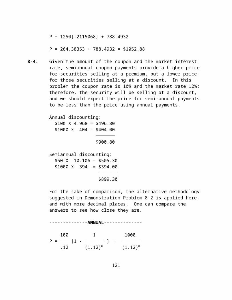
change in bond price due to a change in yield. As such, modified duration measures a bond's sensitivity to interest rate changes and its exposure to interest rate risk.
Convexity indicates the extent to which duration is affected by the curvature of the price/yield relationship. That is, in conjunction with duration, convexity shows how much more bond price will rise with a drop in yield and how much less price will fall with an increase in bond yield. As such, convexity acts to adjust duration so that when used together they provide a more complete measure of bond price volatility.
Price-yield relationship is fundamental to bond price behavior and is based on the principle that bond prices and yields move in opposite directions. This principle is derived from the fact that the price of a bond is equal to the present value of its future cash-flows. That is, a change in yield mathematically must produce an off-setting change in price in the opposite direction. Because present value is an exponential function, the price-yield relationship is convex, meaning that bond prices rise at an increasing rate when yields fall and decline at a decreasing rate when yields rise. Because the relationship is non linear, both duration and convexity are needed to accurately represent bond price behavior.
Now, because duration is the first derivative of bond price with respect to yield, it is represented by a straight line tangent to the price-yield relationship at a given bond yield. As such, the rate of change in bond price estimated by duration remains the same for all changes in bond yields. Duration alone underestimates price appreciation (when rates fall) and overestimates price depreciation (when rates rise). While this is not much of a problem for small changes in yield, the differences can become substantial for large differences.
Because convexity is the second derivative (of price
137
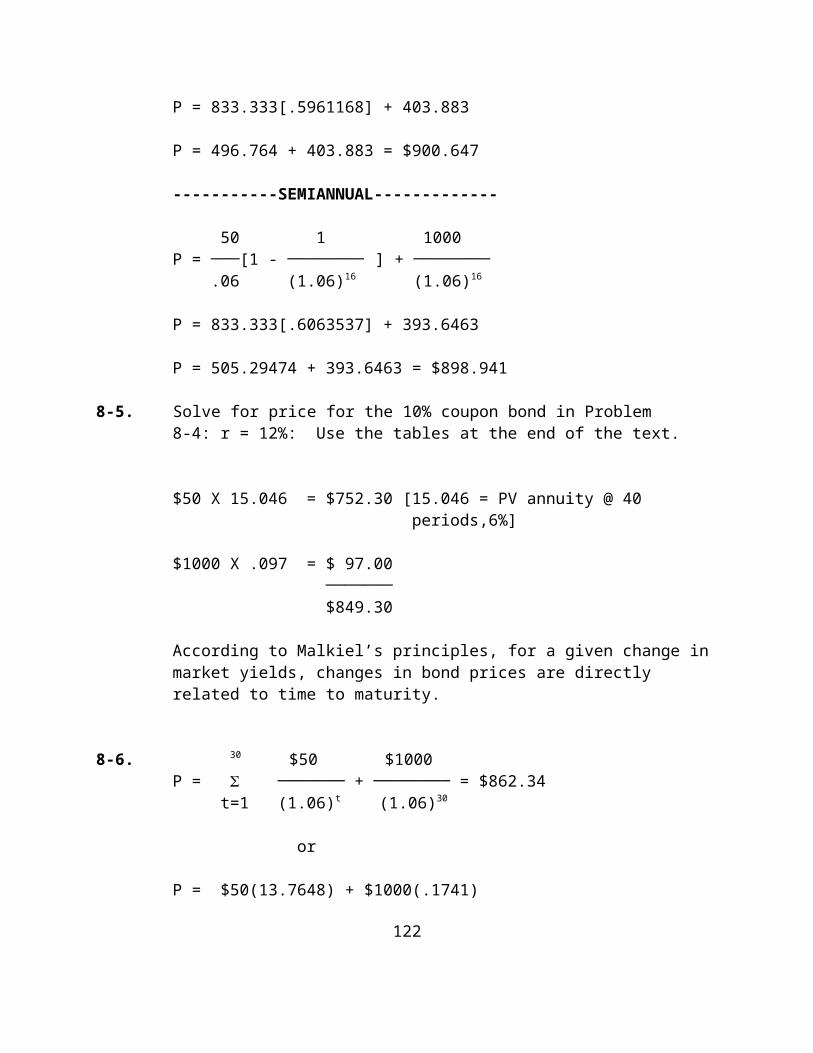
with respect to yield), it results in a curved price-yield relationship which much more accurately reflects bond price behavior. Essentially, convexity is used with duration to correct errors in estimated price behavior, especially with large swings in yields. That is:
Price Change Estimated by Duration + Adjustment in Price Change Due to
Convexity= More Accurate Measure of Price Change
As can be derived from the discussion above, the best way to monitor bond price volatility, whether individually or in a portfolio, is to use BOTH duration and convexity. Duration is fine for small moves in yield, but as the change in yield increases (to more than 100 basis points or so), the combination of both duration and convexity provides the superior measure of estimated bond price behavior.
B. A barbell portfolio combines two bonds such that the portfolio has the desired (bullet) modified duration. The term barbell comes from the usual practice of combining bonds at opposite ends of the term structure. The motivation for a barbell position is to manage the convexity of the investment.
The barbell position is a combination of the two bonds, such that the weighted modified duration is eight years:
3.97 w1 + 9.73 (1 - w1) = 8.0
w1 = .30 (bond 1)
w2 = .70 (bond 2)
138
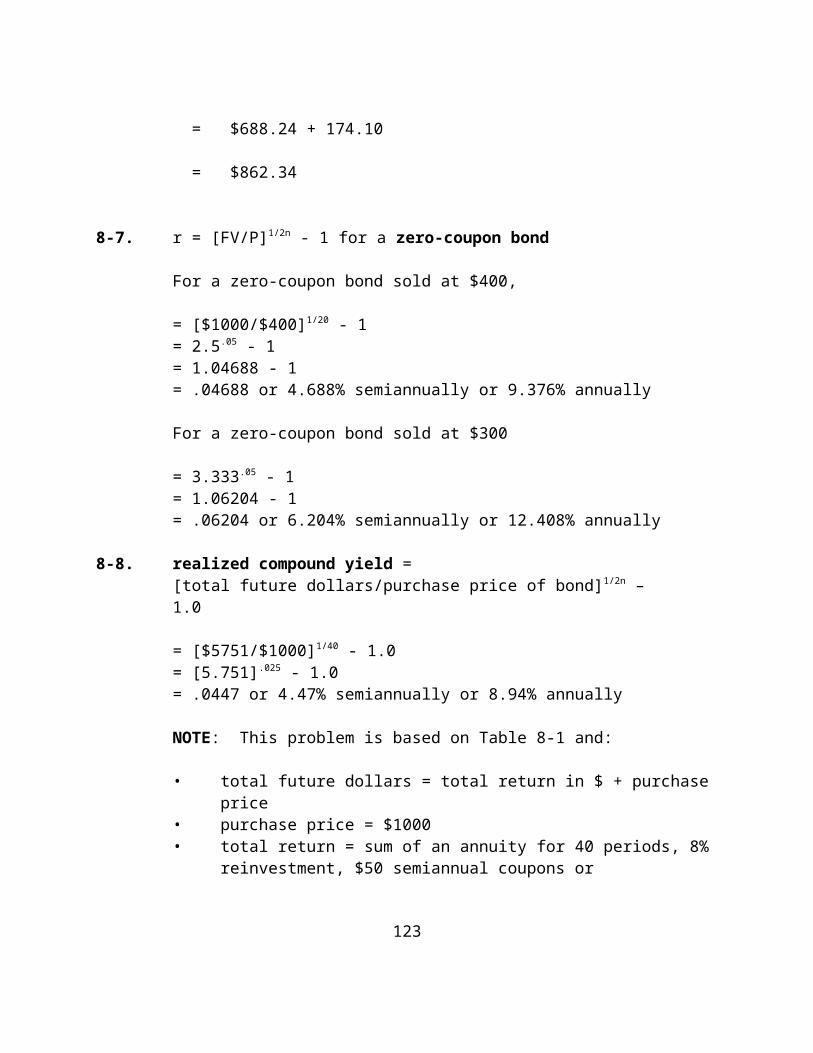
Mod. Wt't. Mod.Bond Weights Duration Duration
1 .30 * 3.97 yrs. = 1.19 yrs. 2 .70 * 9.73 yrs. = 6.81 yrs. 1.00 8.00 yrs. ═════════
At the same time, this barbell portfolio will also have its own weighted average convexity:
Wt'd. Avg.Bond Weights Convexity Convexity
1 .30 19.58 5.87 2 .70 167.56 117.29 1.00 123.16 ══════
Thus, the two positions stack up as follows:
Mod. Duration Convexity15-year T-Bond Currently Held 8.0 years 94.36Proposed Barbell Portfolio 8.0 years 123.16
Clearly, while the two positions result in the same duration, the convexity of the barbell is considerably higher than the bond currently held. The net result is that the price behavior of these two positions will not be the same over different yield environments. More specifically, the two positions will undergo about the same price volatility if rates drop by only 50 basis points, since the durations are the same and convexity doesn't have much of an impact with small swings in yields. In sharp contrast, if rates drop by 250 basis points, the barbell will experience much better price appreciation, as the larger convexity will lead to more price volatility. All of this, of course, assumes an equal shift in the term structure --i.e., that both 5-year and 30-year issues experience the same change in yield. If they don't, the price behavior could differ -- not because of
139
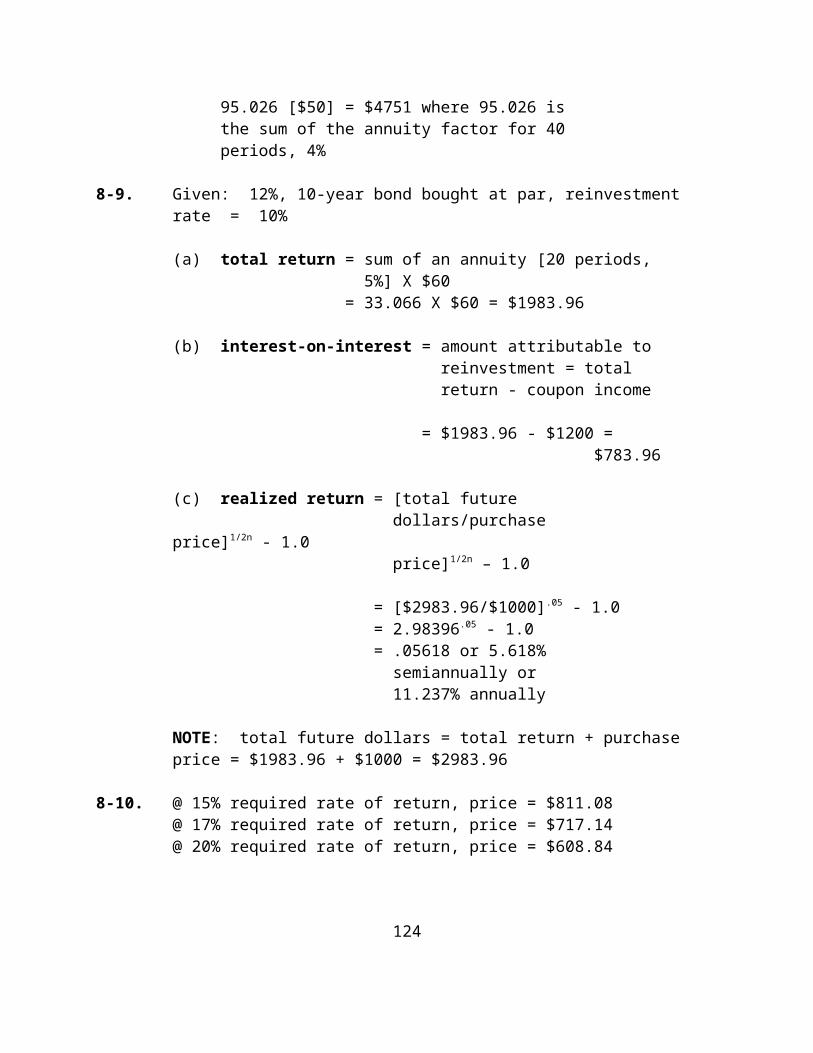
variations in convexity, but because of variations in yield behavior.
CFA9-3. The three reasons for these discrepancies that could be
cited from the information provided are:
1. Modified duration, when used to estimate the expected price behavior of a bond, is only accurate for small changes in yield. The relatively large 100 basis point change assumed in the question accentuates this fact. The inaccuracy of modified duration as an estimator of percentage price change is referred to as convexity. Therefore, convexity is a measure of the degree to which modified duration (a linear estimate of price sensitivity) fails to capture the true dynamics of the curvilinear price/yield function.
2. The percentage volatility indicated by the modified duration number applies to the full price of the bond including accrued interest, and not the quoted (flat) price. Here, only market quoted prices have been used (excludes accrued interest).
3. The effect of a call price is shown by examining Bond Z. Since Bond Z only rose in price by 2.4% (to 101), it is obvious that the price rise has been constrained by the greater likelihood of it being called at par (100) in one year on June 1, 1990.
Although no specific information is provided in the question, two other possible sources of discrepancy are:
4. A change in tax rate could impact market prices, so that their change would vary from the amount predicted by the modified duration number.
5. Differences in market liquidity could impact the changes in market price of the three bonds. Supply and demand considerations could affect one type of bond more significantly than another.
140
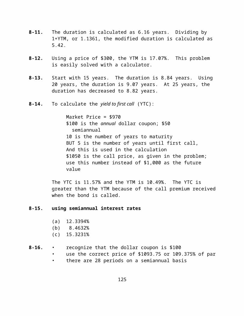
Chapter 10: Common Stock Valuation
CHAPTER OVERVIEW
141

Similar to the two chapter sequence on bonds, there are two chapters on common stocks involving first the valuation of the asset, followed by analysis and management. In addition, the chapter on efficient markets has been moved to Part IV because the concept is almost entirely concerned with stocks as far as students in a beginning Investments course are concerned.
Chapter 10 is one of the most important chapters in the text. It covers the valuation of common stocks in detail, including both the discounted cash flow approach and the P/E ratio approach. Clearly, students should know how to find the intrinsic value of a stock using the capitalization of income approach--that is, they should know how to use the Dividend Discount Model. The eighth edition has been expanded to discuss other discounted cash flow approaches.
The chapter opens by explaining the present value approach again (this was also done in Chapter 8 with bonds). This capitalization of income method seeks to determine the value of a security (its intrinsic value) by discounting all expected future cash flows using a required rate of return. This discussion also includes a brief consideration of the required rate of return (explained in detail in Chapter 11) and the expected cash flows.
The chapter emphasized the classic Dividend Discount Model, which is fully developed, including the three growth rate cases: no growth, constant growth, and multiple growth. However, some of this material has been moved to an Appendix. Numerous examples are provided throughout. The purpose of this analysis is to provide students with the necessary knowledge to work valuation problems, which are found at the end of the chapter.
Relative valuation models are discussed, with primary emphasis on the P/E ratio model. The P/E ratio approach is explained as an alternative way of doing fundamental analysis, and one that many practicing analysts use. The determinants of the P/E ratio, using the constant growth model, are examined. The relationship between P/E ratios and interest rates is considered. Finally, this approach is contrasted to the Dividend Discount Model.
Other valuation techniques are briefly examined, including price to book and price/sales ratio. These other techniques
142
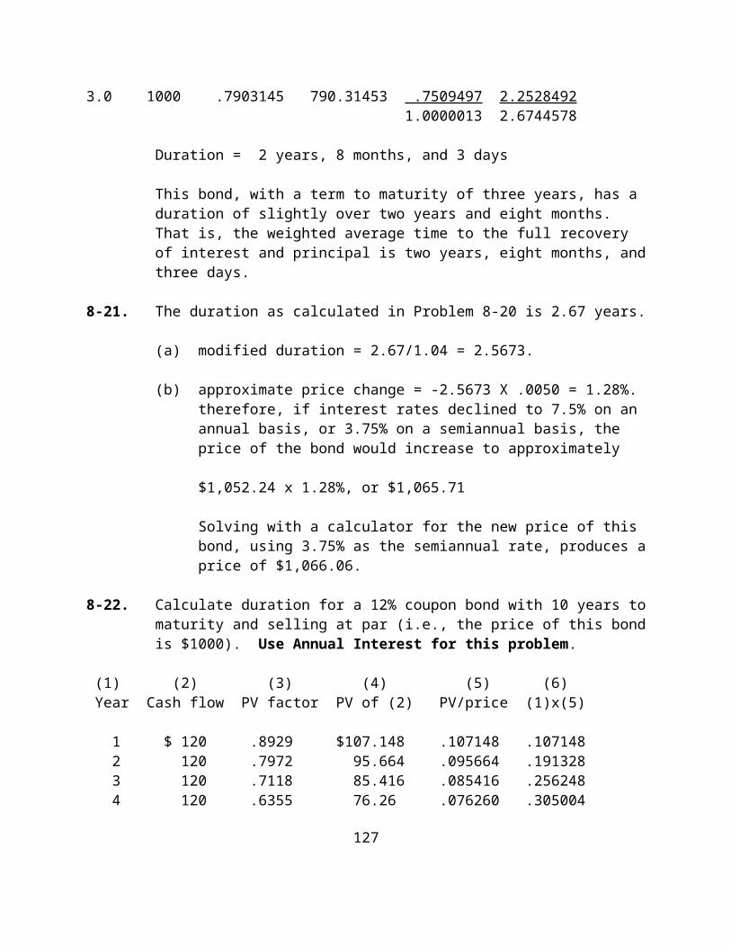
deserve some discussion, but the principal focus remains on the discounted cash flow techniques and the P/E ratio model.
CHAPTER OBJECTIVES
To explain the nature of fundamental security analysis as it applies to common stocks.
To explain discounted cash flow models in general, and the Dividend Discount Model in particular.
To explain relative valuation techniques, with special emphasis on the P/E ratio model.
To establish a framework for fundamental analysis that is used in the three chapter sequence on fundamental analysis (the first three chapters in Part V).
143
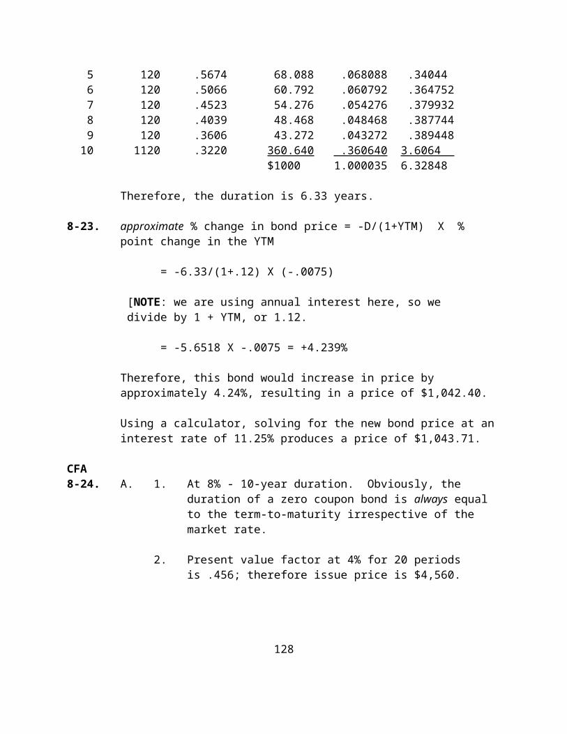
MAJOR CHAPTER READINGS [Contents]
Discounted Cash Flow Techniques
[the discounted cash flow (present value) equation]
The Required Rate of Return [brief description of what it is; more detail in Chapter 11]
The Expected Cash Flows[brief description of what is involved]
The Dividend Discount Model[the equation; the 3 growth rate cases]
Dividends, Dividends--What About Capital Gains?[how dividends plus a terminal price are equivalent to the estimated stream of all future dividends]
Intrinsic Value and Market Price[what it is and what it means; rules for stock selection]
The Dividend Discount Model in Practice [an example of real-world use of this model]
Other Discounted Cash Flow Approaches [Streetsmart Guide to Valuing a Stock]
The P/E Ratio or Earnings Multiplier Approach to Valuation
[model; definition; importance]
The Valuation Model [how this information is presented]
Determinants of the P/E Ratio[factors that affect the P/E ratio; how affected; examples]
Understanding the P/E Ratio[P/Es reflect investor expectations about growth prospects and the risk involved]
P/E Ratios and Interest Rates
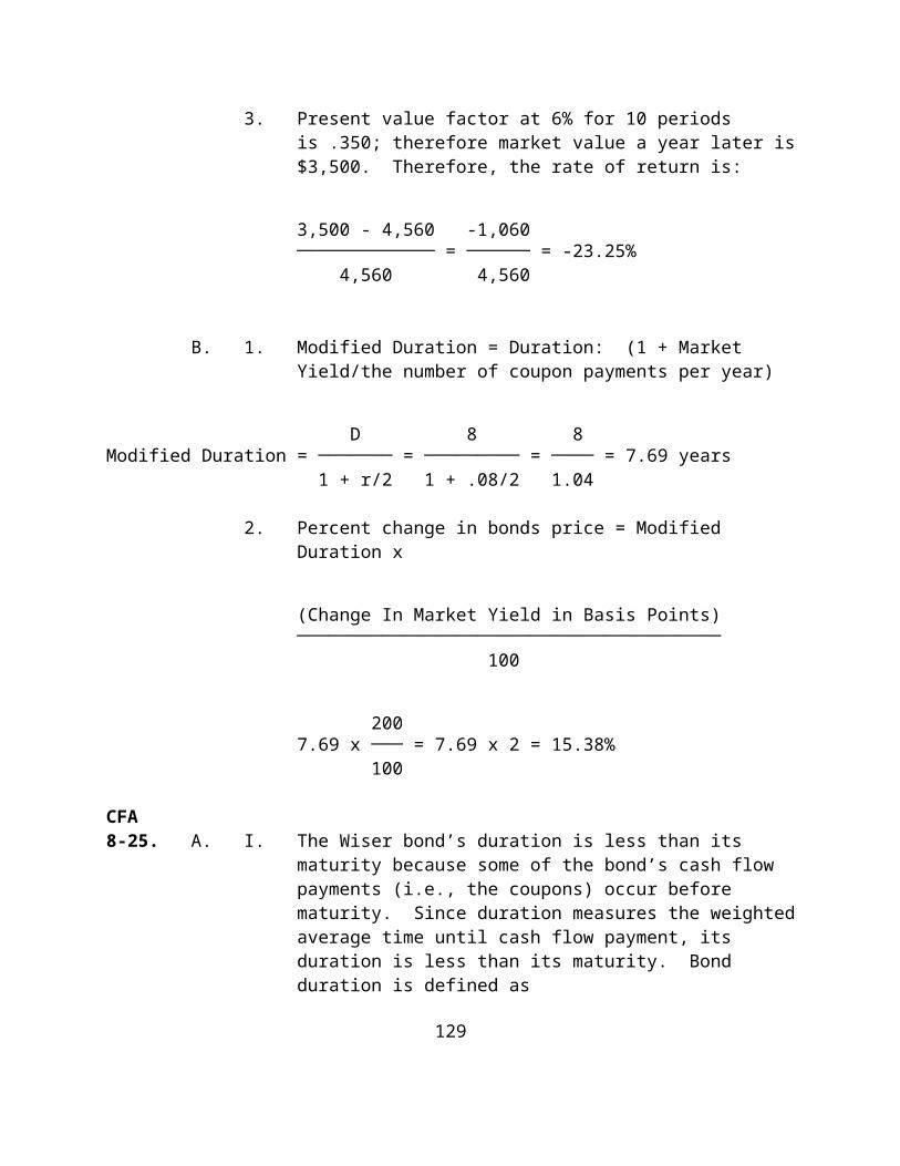
P/E ratios and interest rates are inversely related]
Relative Valuation Techniques
[based on making comparisons in order to determine value]
P/E Ratios[is the P/E for a stock lower or higher than justified by its prospects?; example]
Price/Book Value[P/E ratios and interest rates are inversely related]
P/S Ratio (PRS)
Economic Value Added
Which Approach to Use?
[both approaches, discounted cash flow techniques and relative valuation techniques, can be used and both involve subjective judgments]
Bursting the Bubble on New Economy Stocks—A Lesson in Valuation
[the debacle in dot.com companies; valuation methods do apply]
Some Final Thoughts on Valuation
[subjective nature of valuation]
Appendix 10-A The Constant Growth Version of the DDM
Appendix 10-B The Analysis and Valuation of Preferred Stock
POINTS TO NOTE ABOUT CHAPTER 10
Tables and Figures
Table 10-2 shows the relationship between yields on bonds and P/E ratios. The general point is that interest rates are directly related to required rates of return, and that as the required rate of return increases (decreases), other things equal, the P/E ratio decreases (increases). Therefore, bond yields and P/E ratios are usually inversely related.
Figure 10-1 is designed to illustrate the present value approach to valuation for organizational purposes. The emphasis is on the determination of intrinsic value, which can then be compared to current market price.
Figure 10-2 illustrates the valuation process for a multiple growth company and could be used as a transparency for the purpose of working through these calculations in class. Most students have genuine difficulty in understanding supergrowth (multiple growth) models.
Exhibit 10-1 shows an actual stock recommendation based on P/E ratios and earnings. Students can clearly see how this information is presented by the investment industry to subscribers of investment advisory services.
Figure 10-3 shows stock market capitalizations and P/E ratios for groups of stocks for the year 1998. In this particular case, the largest stocks commanded the highest P/Es.
Figure 10-1A (Appendix) illustrates the constant growth model using a specific example developed in the text (see Table 10-1A). The point here is to show how the nominal value of dividends grows over time as compared to the present value of the dividends.
Table 10-1A illustrates in detail the constant growth version of the Dividend Discount Model by showing year-by-year results for a particular set of inputs. Shown are the dollar dividend, the PV factor, and the PV of the dollar dividend. Because of the format of the equation, many students fail to recognize that the constant growth version involves a present value process and accounts for all dividends from now to infinity.
Box Insert
Box 10-1 is an interesting popular press discussion of the DDM and how it can be used to select stocks, particularly with regard to equation 10-9.
ANSWERS TO END-OF-CHAPTER QUESTIONS
10-1. The intrinsic value of an asset is its fair economic value as estimated by investors. This value is a function of underlying economic variables--specifically, expected returns and risk.
Traditionally, intrinsic value is determined through a present value process. The future expected cash flows on an asset are discounted at a required rate of return.
10-2. The required rate of return for a stock is the minimum expected rate of return necessary to induce an investor to purchase a stock. It accounts for opportunity cost and the risk involved for a particular stock. If an investor can expect to earn the same return elsewhere at a lesser risk, why buy the stock under consideration? Or, put another way, if your opportunity cost for a given risk level is 15%, you should not purchase a stock with that risk level unless you can expect to earn 15% or more from that stock.
10-3. Earnings cannot be used directly in the present value approach because reinvested earnings would be double counted, first as earnings reinvested currently and later as dividends paid. If properly defined and separated, these two variables will produce the same results. Dividends, however, can be used directly.
10-4. The Dividend Discount Model is a widely used method to value common stocks. A present value process is used to discount expected future dividends at an appropriate required rate of return. The equation is:
D1 D2 D3 D
PVcs = ───── + ────── + ────── + ... + ────── (1+k) (1+k)2 (1+k)3 (1+k)
10-5. The problems encountered in the dividend discount model stated as Equation 10-2 in the text, and shown above in answer number 10-4, include:
(a) The last term indicates we are dealing with infinity.(b) The dividend stream is uncertain.(c) The required rate of return has to be determined.
10-6. The three possibilities for dividend growth are:
(a) no growth--the dollar dividend will remain fixed.
(b) constant growth--the dividend will grow at a steady (constant) rate over time.
(c) multiple (super growth)--at least two different growth rates are involved. Many multiple-growth-rate companies grow rapidly for some years and then slow down to a more normal growth rate.
The constant growth model is probably the most applicable to the typical large common stock, and certainly is more often used, rightly or wrongly (because of its simplicity). The no-growth case is the least likely to apply.
10-7. Although dividends are paid to infinity, they can be modeled as either (ignoring the no-growth case) a constant growth rate or a supergrowth situation involving rapid growth for some years plus a constant growth situation for the remainder. In either case, the infinity sign is eliminated.
On a practical basis, after 30 or 40 years dividends discounted at rates of 10% to 20% (or higher) will have insignificant value and can be ignored.
10-8. The dividend discount model can be stated as:
Dt
(a) P0 = ────── t=1 (1+k)t
where P0 is the current market price of the stock. Alternatively, we could say
n Dt Pn
(b) P0 = ────── + ────── t=1 (1+k)t (1+k)n
In (b), Pn is a function of all dividends to be paid from n+1 to infinity, or

Dt
(c) Pn = ────── n+1 (1+k)t
Substituting the right-hand side of (c) into (b) for Pn produces (a), putting us back to where we started. Therefore, the combination of a specified number of dividends and a terminal price is exactly equivalent to an infinite number of dividends because the terminal price takes up where the specified number of dividends stopped (i.e., it is equal to the discounted value of all future dividends).
10-9. The two investors are likely to derive different prices because:
(a) They will probably use different estimates of g, the expected growth rate in dividends.
(b) They are likely to use different required rates of return.
10-10. Investors compare intrinsic value (IV) to the current market price (CMP) of the stock.
If IV > CMP, the stock is undervalued -- buy
If IV < CMP, the stock is overvalued -- sell
If IV = CMP, the stock is correctly valued and in equilibrium.
10-11. P/E ratios shown daily in The Wall Street Journal reflect the current market price of the stock divided by the latest 12 month earnings. Therefore, they show only the current multiple for a stock. While this can be a useful reference point, investors seeking to value a stock will need an estimate of the future multiplier.
10-12. The P/E ratio is affected by:
(a) The expected dividend payout ratio (D/E).(b) The required rate of return.
(c) The expected growth rate of dividends.
The P/E ratio is quite sensitive to a change in these factors. A one percentage point change in the required rate of return, for example, can easily change the price of a stock 30 or 40%. A one percentage point change in g, the expected growth rate of dividends, also has a significant impact, but not as large as a change in the required rate of return. Both of these factors usually have more impact than the payout ratio.
10-13. Some analysts argue that the dividend discount model is unrealistic because it requires a forecast of dividends into the distant future (technically, infinity). Also, many investors are seeking capital gains, while this model seemingly focuses on dividends. In response, it should be noted that the dividend growth rate can be modeled in a workable manner, avoiding the infinite horizon problem. Furthermore, investors can structure a stream of dividends and a terminal price (which allows for capital gains) and have an alternative that is equivalent to the basic model.
Perhaps the most important point here is that either model, the dividend discount model or the multiplier model, requires estimates of the future. These estimates cannot be avoided! Whether the inputs for one model as opposed to the other model are more realistic is probably an unresolvable argument.
10-14. This analysis is based on the equation (D/E)/(k-g).
(a) decline
(b) decline
(c) increase
(d) increase*
*the riskless rate of return is a component of the required rate of return, which has an inverse relationship with the P/E.

ANSWERS TO END-OF-CHAPTER PROBLEMS
10-1. Using the constant growth version of the Dividend Discount Model:
k = D1/P0 + g
= $2.00/$45 + .09
= .1344 or 13.44%
10-2. Reversing the formula used in answer 10-1 to solve for price, and recognizing that we must compound the stated dividend, D0, up one period to obtain D1,
P0 = D1/(k-g)
= D0(1+g)/(k-g)
= $2.25(1+.08) / (.13-.08)
= $2.43/.05
= $48.60
10-3. Again using the constant growth version of the Dividend Discount Model, solve for g
k = D1/P0 + g k-g = D1/P0
-g = D1/P0 - k g = k - D1/P0
Or: g = k - [(D0(1+g))/P0]
Therefore: g = .15 - [($3.00(1+g))/50] 50g = 7.50 - 3 - 3g 53g = 7.50 - 3 53g = 4.50 g = 08.49 or 8.49%
10-4. P = D0/k = 1.50/.15 = $10.00
10-5. (a) k = D0/P0 = $3.00/$40 = 7.5%
159

(b) The price will decline because required rates of return rise while dividends remain fixed.
Specifically,
P = $3.00/.09 = $33.33
10-6. Given a one year horizon, this problem can be formulated as
D1 P1
P0 = ─────── + ─────── (1+k) (1+k)
$25 = $3.00/(1+k) + $30/(1+k) (1+k)25 = 3 + 30 1+k = 33/25 =1.32 k = 32%
10-7. (a) (1) Stock A kA = RF + ßA (RM-RF) = .10 + 1.0(.15 -.10) = .15
(2) Stock B kB = .10 + 1.7(.15-.10) = .185
(3) Stock C kC = .10 + .8(.15-.10) = .14
(b) If RF increases to .12, required rates of return are:
kA = .12 + 1.0(.03) = .15
kB = .12 + 1.7(.03) = .171
kC = .12 + 0.8(.03) = .144
(c) If RM increases to 17%, the required rates of return also rise. The new results are:
kA = .10 + 1.0(.17-.10) = .17
kB = .10 + 1.7(.17-.10) = .219
160
kC = .10 + 0.8(.17-.10) = .156
10-8. (a) It is necessary to calculate the growth rate since it is not given. Referring to the future (compound) value table at the end of the text, and reading across the 12 year row, we find a factor of about 2.0 (actually, 2.0122) at the intersection of the 6% column (or, using the rule of 72, 72/12 = 6%). Therefore g = 6% and
k = [$3.00(1.06)]/$60 + .06 = 053 + .06 = .113 or 11.3%
(b) Using the same table to find a factor of 3.0 on the 6 year row, we find g to be approximately 20% (the exact factor at 20% is 2.986). Therefore, using g = 20%,
k = [$3.00(1.20)]/$60 + .20 = .06 + .20 = .26 or 26%
10-9. (a) Solving for k as the expected rate of return,
k = [$1.80(1.08)]/$36 + .08 = .054 + .08 = .134 or 13.4%
Since the expected return of 13.4% is less than the required rate of return of 14%, this stock is not a good buy.
(b) P0 = D1/(k-g) = [$1.80(1.08)]/[.14-.08] = $32.40
An investor should pay no more than $32.40 if his or her required rate of return is 14%.
If the required rate of return is 15%, the maximum an investor should pay is obviously less than in the previous problem. Specifically,
161
P0 = [$1.80(1.08)]/[.15-.08] = $27.77
10-10. (a) The current P/E ratio is $32/$4 = 8
(b) E0 = $4
E1 = E0(1+g) = $4(1+.10) = $4.40
With an unchanged P/E of 8, the new price will be
8 x $4.40 = $35.20
(c) D/E = 50% -- payout ratio g = 10% -- expected growth rate of dividends k = 16% -- required rate of return
expected rate of return = D1/P0 + g = $2.20/$32 + .10 = .169 or 16.9%
Alternatively,
P0 = D1/(k-g) = $2.20/(.16-.10) = $36.66
This stock is a good buy because the expected return exceeds the required return or, alternatively, the estimated value (price) of the stock exceeds the current market price.
(d) If interest rates are expected to decline, the likely effect is an increase in the P/E ratio for Joy Juice as well as other stocks.
10-11. $1.30 (1.11) ──────────── = $30.38
162
15.75 - .11
10-12. $1.30 (1.16) ──────────── = no solution 15.75 - .16
This problem cannot be solved using this equation because the growth rate is greater than the discount rate (required rate of return).
10-13. Using any computer package that solves stock valuation problems, the correct price of $32.29 should be produced.
10-14. This problem is a 3-stage growth model, which is solved exactly as in 10-13 except three growth rates and the time periods covered are entered rather than two. The program will produce a price for this stock of $27.50.
10-15. Lowering the growth rate in the first supernormal growth period from 30% to 25% will clearly result in a lower price because of the lesser growth rate in dividends and the lesser dollar value of the resulting dividend stream. Making this one change(obviously, no other changes are necessary) results in a new price of $23.08.
10-16. D0 = $1.60; k = 16%; g = 8%
$1.60 (1.08) $1.73P0 = ──────────── = ───── = $21.63 .16 - .08 .08
10-17. $2.00 (.40) = $0.80 = D1
The correct growth rate to use is the expected growth rate of 7%.
$0.80P0 ─────── = $10 .08
10-18. P0 = $0.60 (.847) + $1.10 (.718) + $1.25 (5.556)
163
(.718) = $0.51 + $0.79 + $4.99
= $6.29
NOTE: 5.556 is 1/.18 (to account for the perpetuity). This value must then be discounted back to today using the 2-year factor since the perpetuity is valued as of the beginning of year three, which is the same as the end of year two.
10-19. D1 = $1.80 (1.06) = $1.91
= .90 (since the stock is 10% less risky than the market)
k = 5% + .9 (7%) = 11.3%
$1.91P0 = ────────────── = $36.04 .113 - .06
10-20. k = D0 / P0
$1.00k = ─────── = 8.33% $12
10-21. k = (D1 / P0)+ g
k = $2.00 (1.07) / $40 + 7% = 12.35%
10-22. P0 = ($3.00/.25)(.328) = $3.94
10-23. k = D1/P0 + g
g = k - D1/P0
g = .10 - $2.00/$50
= .06
10-24. P0 = $10 (4.192) + $15 (5.00) (.162)
= $41.92 + $12.15 = $54.07
164

NOTE: 4.192 is the present value of an annuity factor for 10 periods at 20%. 5.00 is the perpetuity factor for 20%, and .162 is the present value factor for 10 periods, 20%.
10-25. This is a 2-stage growth model, or supergrowth. Find the present value of all dividends from now to infinity.
n D0(1+g1)t Dn(1+gc) 1 P0 = ─────────── + ────────── ──────── t=1 (1+k)t k-gc (1+k)n
where g1 is the supergrowth rate in dividends, gc is the constant growth rate, and n is the number of years of supernormal growth. Solving for the present value of the dividends for the first five years of supergrowth:
PV D0 = $1.00 PVIF.18 in $ D1 = 1.00(1.25) = $1.25 .847 $1.06 D2 = 1.00(1.25)2 = 1.56 .718 1.12 D3 = 1.00(1.25)3 = 1.95 .609 1.19 D4 = 1.00(1.25)4 = 2.44 .516 1.26 D5 = 1.00(1.25)5 = 3.05 .437 1.33 PV of dividends for first 5 years = $5.96
D5(1+gc) $3.05(1.07) $3.26 P5 = ──────────── = ─────────────── = ───────── = $29.67 k-gc .18 - .07 .11
We must discount P5 back to time period zero and add this value to the present value of the first five years of dividends.
NOTE: P5 is the price at the end of year five; therefore, we use the discount factor for 5 years, not 6 years.
P5 discounted to time period zero: P5 (PVIF.18,5) = $29.67(.437) = $12.97 P0 = $5.96 + $12.97 = $18.93
10-26. This is a three stage growth model. It is unusual in that in the second stage of growth, the growth rate is equal to the discount rate. The process remains the same.
165
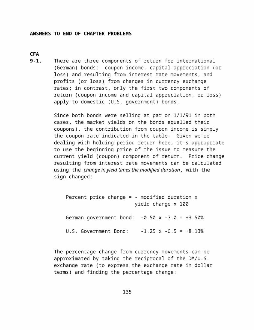
D0 = $2.00 PVIF.20 PV in $ D1 = 2.00(1.30) = $2.60 .833 $ 2.17 30% = g D2 = 2.00(1.30)2 = 3.38 .694 2.35 D3 = 2.00(1.30)3 = 4.39 .579 2.54----------------------------------------------------------- D4 = D3(1.20) = $4.39(1.20) = $5.27 .482 2.54 D5 = D4(1.20) = 5.27(1.20) = 6.32 .402 2.5420% = g D6 = D5(1.20) = 6.32(1.20) = 7.58 .335 2.54 D7 = D6(1.20) = 7.58(1.20) = 9.10 .279 2.54 D8 = D7(1.20) = 9.10(1.20) = 10.92 .233 2.54 ────── $19.76
D8(1.06) $10.92(1.06) $11.58 P8 = ───────── = ──────────── = ────── = $82.71 .20 - .06 .14 .14
Discounting P8 back eight periods:
$82.71(.233) = $19.27
P0 = $19.76 + $19.27 = $39.03
10-27. This is a case of three years of zero dividends, followed by a no-growth period of infinite length. Note that one year prior to the start of the no-growth period is year 3. Therefore,
P3 = D/k = $1/.14 = $7.14
P0 = P3 (PVIF.10,3) = $7.14 (0.675) = $4.82
CFA D1
10-28. a. VALUE0 = ------ K - g
D1 = next year’s dividend
K = required rate of return
166

g = constant growth rate
D1 = (EPS0)(1 + g)(P/0) = (4.50)(1.045)(.55) = $2.59
K = given at 11% or .11
g = (ROE)(1 - P/0) = (.10)(1 - .55) = .045
$ 2.59 $2.59VALUE0 = ──────── = ────── = $39.85 .11-.045 .065
b. Multistage Dividend Discount Model (where g1 = .15 and g2 is .045):
D1 D2 D3/(K-g2)VALUE1 = ───── + ────── + ───────── (1+K) (1+K)2 (1+K)2
D1 = (EPS0)(1 + g1)(P/0) = (4.50)(1.15)(.55) = $2.85
D2 = (D1)(1 + g1) = ($2.85)(1.15) = $3.27
K = given at 11% or .11
g2 = .045
D3 = (D2)(1 + g2) = ($3.27)(1.045) = $3.42
VALUE0 = $2.85 $3.27 3.42/(.11-.045) ────── + ─────── + ─────────────── (1.11) (1.11)2 (1.11)2
$2.85 $3.27 $52.62 ────── + ─────── + ─────── (1.11) (1.11)2 (1.11)2
= $2.56 + $2.65 + $42.71
= $47.92
CFA
167
10-29. d(a) The dividend discount model is: P = ───── k - g
Where P - value of the stock today d - annual dividend one year forward
k - discount rate g - constant dividend growth rate
d dSolving for k: (k - g) = ───; then k = ─── + g p p
So k becomes the estimate for the long-term return of the stock.
$.60k = ────── + 8% = 3% + 8% = 11% $20.00
(b) Many professional investors shy away from the dividend discount framework analysis due to its many inherent complexities.
(1) The model cannot be used where companies pay very small or no dividends and speculation on the level of future dividends could be futile. (Dividend policy may be arbitrary.)
(2) The model presumes one can accurately forecast long term growth of earnings (dividends) of a company. Such forecasts become quite tenuous beyond two years out. (A short-term valuation may be more pertinent.)
(3) For the variable growth models, small differences in g for the first several years produce large differences in the valuations.
(4) The correct k or the discount rate is difficult to estimate for a specific company as an
168
infinite number of factors affect it which are themselves difficult to forecast, e.g., inflation, riskless rate of return, risk premium on stocks and other uncertainties.
(5) The model is not definable when g > k as with growth companies, so it is not applicable to a large number of companies.
(6) Where a company has low or negative earnings per share or has a poor balance sheet, the ability to continue the dividend is questionable.
(7) The components of income can differ substantially, reducing comparability.
(c) Three alternative methods of valuation would include:
(1) Price/Earnings ratios(2) Price/Asset value ratios (including market and
book asset values)(3) Price/Sales ratios(4) Liquidation or breakup value(5) Price/cash flow ratios
CFA10-30. A. The formula for the constant growth discounted
dividend model is shown below:
D0 (1 + g) Price = ──────────── k - g
Where D0 = current dividends per share
For Eastover:
1.20 * 1.08Price = ───────────── = 43 0.11 - 0.08
This compares with its current stock price of 28. On this basis, it appears that Eastover is undervalued.
169

B. The formula for the two-stage discounted dividend model is as follows:
D1 D2 D3 P3
Price: ───── + ─────── + ─────── + ─────── 1+k (1+k)2 (1+k)3 (1+k)3
D4
where P3 = ──────── k - g2
For Eastover: g1 = .12 g2 = .08
D0 = 1.20D1 = 1.20 * 1.12 = 1.34D2 = 1.20 * (1.12)2 = 1.50D3 = 1.20 * (1.12)3 = 1.69D4 = D3 * (1.08) = 1.82
P3 = 1.82 / (.11 - .08) = 60.67
1.34 1.50 1.69 60.67Price = ──── + ─────── + ─────── + ─────── 1.11 (1.11)2 (1.11)3 (1.11)3
= 48.03
This approach indicates that Eastover is even more undervalued than was the case with the constant growth approach.
An alternative solution to two-stage model is:
D1 D2 P2
Price = ───── + ────── + ────── (1+k) (1+k)2 (1+k)2
D3 1.69P2 = ──── = ─────── = 56.33 k-g2 .11-.08
1.34 1.50 56.33
170
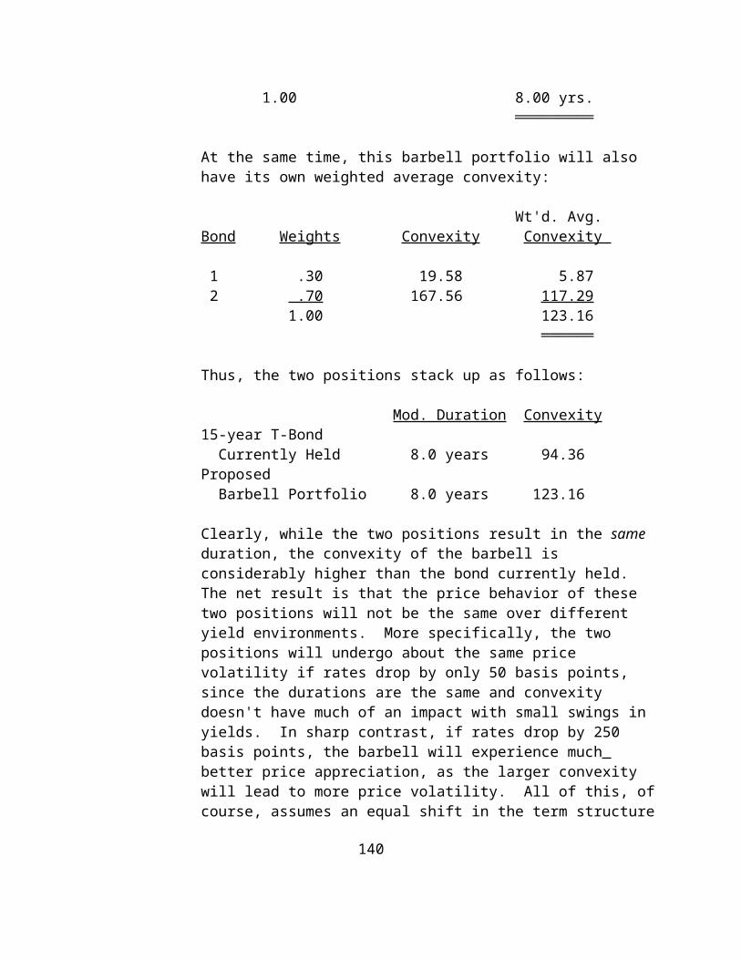
Price = ──── + ─────── + ──────── 1.11 (1.11)2 (1.11)2
= 1.21 + 1.22 + 45.72
= 48.15
This answer differs from previous answer because of round off error.
C. Constant growth model:
Advantages: 1) logical, theoretical basis2) simple to compute3) inputs can be estimated
Disadvantages: 1) very sensitive to inputs of growth
2) g and k difficult to estimate accurately
3) result is meaningless if g > k4) constant growth is an
unrealistic assumption5) assumes growth will never slow
down6) dividend payout must remain
constant7) not usable for firms not
paying dividends8) assumes stock price will
increase at g
Improvements with the two-stage model:
1. The two-stage model is more realistic. It accounts for low, high, or zero growth in the first stage, followed by constant long-term growth in the second stage.
2. The model can solve for stock value when the growth rate in the first stage exceeds the required rate of return.
171
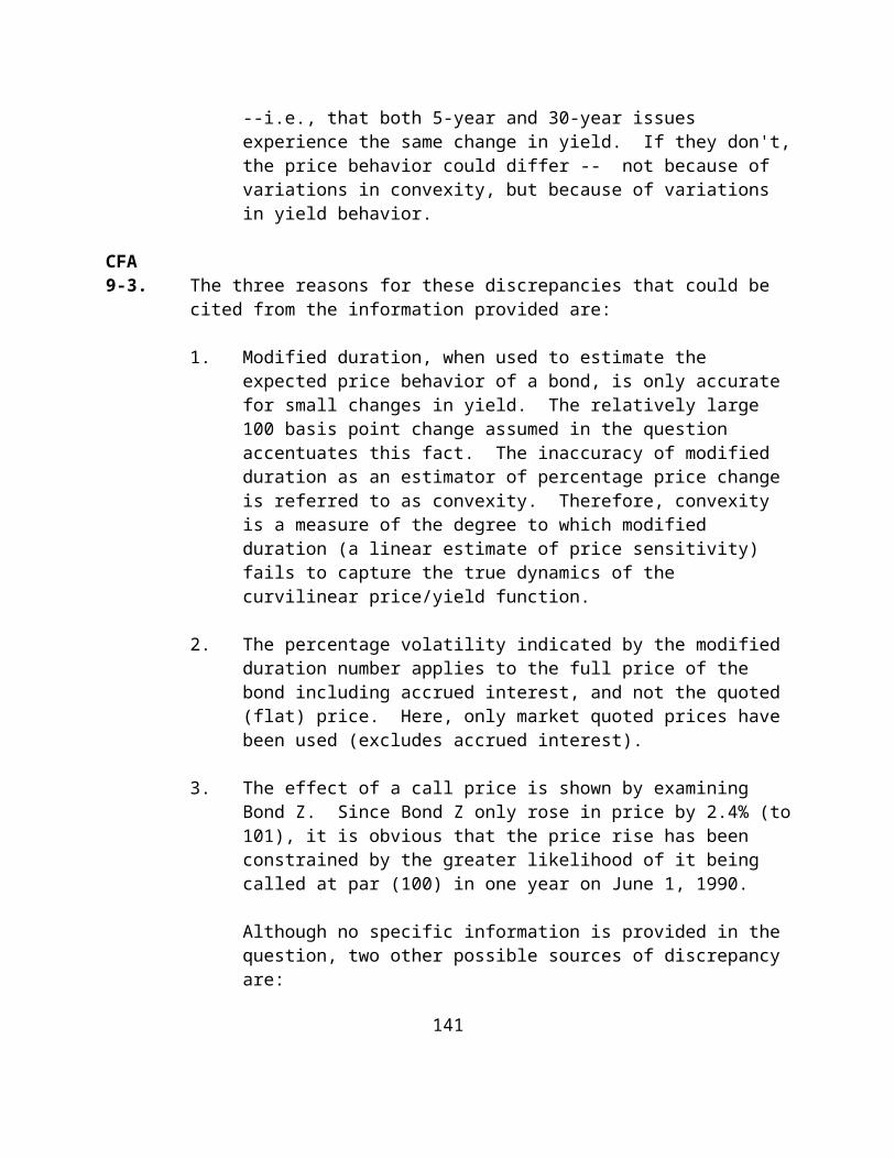
Chapter 11: Common Stocks: Analysis And Strategy
CHAPTER OVERVIEW
Chapter 11 completes a two-chapter sequence on the analysis, valuation, and management of common stocks--the same sequence used earlier for bonds. This chapter concentrates on issues important to the analysis and management of common stocks, given that the valuation of stocks was discussed in Chapter 10. Market efficiency is covered in Chapter 12.
This arrangement allows us to efficiently cover common stocks by discussing valuation in Chapter 10, analysis and management in Chapter 11, and market efficiency in Chapter 12. This provides an in-depth discussion of common stocks that in many cases will suffice for an introductory course; that is, instructors may choose to forego Part V on security analysis, or cover it in less detail. Students will be exposed to the basic terminology, ideas, and concepts involving common stocks by covering these three chapters.
Chapter 11 begins by analyzing common stocks in terms of the impact of the market on common stocks (obviously a major consideration) and in terms of the required rate of return for common stocks (a very important concept covered briefly in earlier chapters). Now that we are analyzing stocks in detail, a full discussion of these two key topics is extremely valuable.
Earlier chapters defined and briefly discussed systematic risk and beta, and we can now emphasize that all investors who plan to analyze and manage a portfolio of stocks must be keenly aware of market risk, both domestic and foreign. In a similar manner, in Chapter 10, in order to concentrate on the techniques of valuation, we assumed that we knew the discount rate or required rate of return. Here we consider it in detail because of its importance to any successful understanding of stocks.
172
Chapter 11 relates to themes developed in Chapter 19, where it is noted that investors often consider the investment decision as consisting of two steps, asset allocation and security selection. We are assuming here that the asset allocation decision has been made.
Following the comparable chapter in the bond sequence (Chapter 9), the discussion of how investors should approach the analysis and management of stocks is divided into the two major alternatives, passive strategies and active strategies. This division is an effective and realistic way to organize this discussion, and once again allows the instructor flexibility in bringing up such topics as Efficient Markets.
The passive strategy discussion covers the buy-and-hold strategy and index funds. The active strategy discussion covers the major alternatives investors have when pursuing an active approach--security selection, sector rotation, and market timing. This discussion is followed by a consideration of how Efficient Markets concepts affect active strategies, and opens up numerous possibilities for discussion.
The remainder of Chapter 11 organizes the analysis of stocks by outlining the approaches to analyzing and selecting stocks--the fundamental approach and the technical approach--which, in effect, organizes the four chapter sequence on security analysis in Part V that follows Chapter 12.
The last section of the chapter provides a framework for fundamental analysis, thereby organizing the first three chapters of the four-chapter sequence in Part V. The recommended order for fundamental security analysis is market/economy, industry, and company analysis.
CHAPTER OBJECTIVES
To concentrate only on the analysis and management of common stocks.
To describe some major concepts and issues that investors should understand when analyzing stocks.
To outline investors’ alternatives in terms of passive and active strategies.
173
To establish a framework for security analysis, which follows in Part V.
174

MAJOR CHAPTER HEADINGS [Contents]
Taking a Global Perspective
[U. S. investors have been myopic]
Analyzing Some Important Issues Involving Common Stocks
The Impact of the Overall Market on Individual Stocks[the significance of market risk; international examples]
The Required Rate of Return[what it is; components; risk and required rate of return]
Building Stock Portfolios
[the asset allocation decision; security selection]
Passive Strategy
[passive strategies seek to do as well as the market]
Buy-And-Hold Strategy[description]
Index Funds[stock-index funds]
The Active Strategy
[assumes investor possesses some advantage relative to others]
Security Selection[the importance of stock selection; the role of the security analyst; forecasting EPS; cross-sectional variation in common stocks]
Sector Rotation[what it involves; examples; use of mutual funds to do this]
Market Timing
[what is involved; evidence on likelihood of success]
Rational Markets And Active Strategies[brief description of the EMH; implications to investors]
Approaches For Analyzing And Selecting Stocks
[framework]
Technical Analysis[brief description; momentum strategies]
Fundamental Analysis[brief description]
Behavioral Finance Implications [brief summary]
A Framework For Fundamental Analysis
Bottom-Up Approach to Fundamental Analysis[definition; growth stocks vs. value stocks]
Top-Down Approach to Fundamental Analysis[definition; rationale for using it here;Economy/Market Analysis; Industry Analysis;Company Analysis]
The Framework for Fundamental Analysis In Perspective[using a diagram to depict the process]
POINTS TO NOTE ABOUT CHAPTER 11
Tables and Figures
There are no tables in Chapter 11.
Figure 11-1 plots the performance of Fidelity’s Magellan Fund, one of the two largest mutual funds in the United States, against the S&P 500 Index for a recent 9-year period. The two track quite closely, illustrating the importance of the market on the performance of diversified portfolios.
Figure 11-2 shows the ex-ante trade-off between required rate of return and risk, as measured by beta. This is always an
important figure to stress to students. The greater the expected risk, the greater the required rate of return.
Figure 11-3 shows the framework for fundamental analysis, setting the stage for the next three chapters (of four) in Part V on security analysis. It indicates that in fundamental analysis investors must estimate the expected cash flows and the risk involved, using either the Dividend Discount Model or the P/E ratio model, and this should be done in the recommended order--market/economy first, industry second, company third.
Box 11-1 is an interesting discussion of security analysts, who occupy a key role in security analysis and the valuation of common stocks. It illustrates that security analysts are often wrong with their recommendations. In 2001 the popular press became much more critical of security analysts and their recommendations, including the “superstars” like Mary Meeker and Henry Blodgett. It is important for students to understand that analysts have traditionally not issued many “sell” recommendations, at least using that word, and that they appear to have often been influenced by the investment banking side of their firm. Because the firm wants to secure or keep a client’s investment banking business, the analyst for that firm may be influenced when issuing opinions about the client’s stock.
ANSWERS TO END OF CHAPTER QUESTIONS
11-1. The market has a major impact on the average stock. For a well-diversified portfolio, which has little or no nonsystematic risk (attributable to individual company factors), the market is the dominant influence on the portfolio, explaining most of the variation in its returns. Since most mutual funds are very diversified, they will tend to move very much like the market.
11-2. Common stock investors recognize that returns will be quite variable on a year-to-year basis. One has only to examine the S&P data given in the text to verify this. Nevertheless, owning common stocks is a prudent thing to do because of their larger returns. Diversification is an absolute essential, which helps to reduce the risk. Also, owning stocks over a long period helps to reduce the risk in the sense that a portfolio does not have to be liquidated during bear market periods. Based on the historical evidence, it would not be prudent to own a portfolio of fixed-income securities over a long period of time because of their much lower returns (and ending wealth), particularly on an inflation-adjusted basis.
11-3. The ownership of foreign stocks is a natural, and important, part of the diversification process as well as the process of seeking the best returns possible, given the risk involved. Investors must operate in an international environment in today’s world.
The fact that Japanese stock prices dropped drastically simply means that for new investors a significant opportunity exists. The question, of course, has been when to buy. For example, Japanese stocks rallied sharply in 1993 from the low point reached but also had problems after that time. As of August, 2001, Japanese stocks were at a 17-year low.
All stock markets are risky, domestic and foreign. 11-4. The required rate of return for IBM is the minimum
expected rate of return necessary to induce investors to purchase IBM shares. The required rate of return takes into account the opportunity cost involved of investing in a particular stock with a given level of risk. In
169
the case of IBM, an investor can justify purchasing shares if he or she can expect to earn a level of return that will adequately compensate for the risk involved as measured by the stock’s beta coefficient.
11-5. The two components of the required rate of return are:
• the risk-free rate of return--available to all investors by buying risk-free assets
• the risk premium--compensation for the particular risk of an asset--the larger the risk, the larger the risk premium
11-6. There are many financial assets and, therefore, many different required rates of return. Within a particular asset category such as common stocks, there are many required rates of return. The level of required rates changes over time.
11-7. The shape of the tradeoff between the required rate of return and risk is upward sloping because the relationship is formulated on an ex-ante basis. That is, investors purchase assets to hold based on their expectations of the future. Ex post, for relatively short periods, this relationship can, and does, slope downward. It does not, however, when long periods of time are considered--for example, data since 1920 clearly shows that stocks return about twice what bonds return over long periods.
11-8. Since the market has a beta of 1.0 by definition, the required rate of return is simply the expected rate of return on the market.
11-9. Passive strategies are based on the proposition that an investor does not possess either the knowledge or the ability to outperform the market as a whole. These strategies simply seek to do as well as the market. Passive strategies are related to the concept of efficient markets.
11-10. Three active strategies for common stocks include:
stock selection--searching for undervalued or
170
overvalued stocks
sector rotation--shifting the sector weights in a portfolio to take advantage of
those sectors expected to do relatively better and avoid those expected to do relatively worse
market timing-- the attempt to earn excess returns by varying the percentage of portfolio assets in equity securities.
11-11. In evaluating common stocks, according to one study, security analysts rely on presentations from top management of companies, annual reports, and Form 10-K reports that the companies must file with the SEC.
11-12. The cross-sectional variation in common stocks is large. In a given year, there is a wide range in performance of stocks. Investors who can confine stock selection to the stocks in the highest quartile in a given year would largely avoid losing years. However, about 25 percent of the time even the best stocks would have lost money. Cross-sectional variation of returns has been increasing steadily over the decades.
11-13. Sector rotation is an active strategy involving shifting sector weights in the portfolio in order to take advantage of those sectors that are expected to do relatively better, and avoid or de-emphasize those sectors that are expected to do relatively worse. Investors using this strategy are betting that particular sectors will repeat their price performance relative to the current phase of the business and credit cycle.
The key to effective strategies involving sector rotation is an accurate assessment of current economic conditions.
11-14. The evidence on market timing suggests that there is little evidence of many investors doing this successfully on a consistent basis. The evidence from mutual funds is particularly persuasive in this regard.
11-15. The Efficient Market Hypothesis has to do with the adjustment of stock prices to new information. If the
171
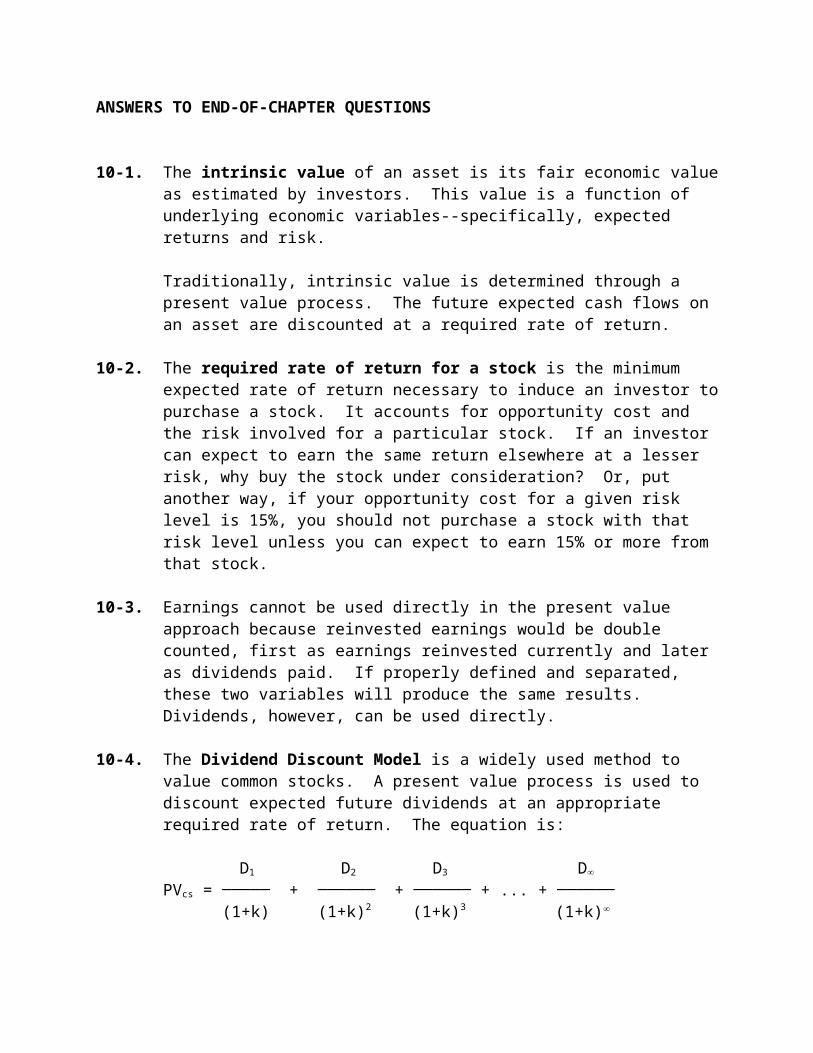
market is efficient, stock prices adjust quickly, and on balance accurately, to new information. This hypothesis has obvious implications for the strategies and approaches discussed in this chapter.
11-16. The implications of the EMH to both stock selectors and market timers is that they are unlikely to be successful unless they have access to information others do not have or they have superior ability and skill. If the market is efficient, prices currently reflect all available information.
11-17. The two traditional approaches to analyzing and selecting common stocks are fundamental analysis and technical analysis. Fundamental analysis uses the fundamental accounting and related data of the firm--sales, earnings, financing, and so forth--to estimate the intrinsic value of a company. Technical analysis uses the past price and volume data for a company or the market as a whole in an attempt to forecast the future price direction, and/or technical indicators.
11-18. The recommended framework for fundamental analysis is market/economy first, industry second, and company third. This is a top-down approach because it starts with the economy/market first and works down to the individual company.
11-19. The top-down approach is consistent with the discussion about the impact of the market on the typical stock, and in particular the typical well-diversified portfolio. If the market is expected to go down, most stocks also can be expected to decline, and it would not be desirable to be assuming long positions at such a time. Thus, it makes sense to analyze the market first, before considering either particular industries or particular companies.
11-20. Fundamental analysis is based on the premise that any security has an intrinsic value, or its true value as estimated by an investor. This value is a function of the firm’s underlying variables, which combine to produce an expected return and an accompanying risk.
172
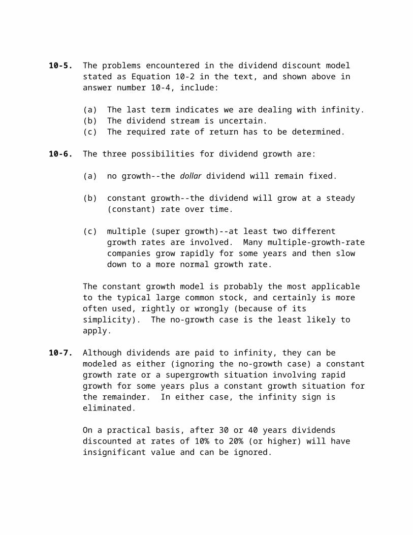
Chapter 12: Market Efficiency
CHAPTER OVERVIEW
A chapter on market efficiency is a natural sequence to the other two chapters in Part IV dealing with common stocks. It is also desirable for students to be familiar with this topic at this point so that market efficiency can be referred to when discussing other topics, such as technical analysis or fundamental security analysis.
Chapter 12 begins by explaining the rationale for arguing that the market is efficient. It then proceeds to outline the
173
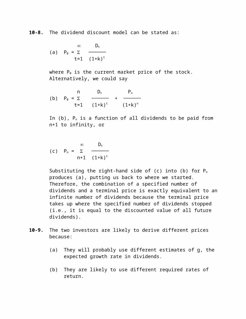
classic three forms of market efficiency laid out by Fama in 1970: weak, semi-strong, and strong.
Evidence on market efficiency is presented in some detail, starting with weak form efficiency and concluding with strong form efficiency. Within the weak form section the distinction is made between statistical tests and trading rule tests. In the semi-strong form section the concept of event studies is developed, along with abnormal returns. Strong form evidence is developed in considerable detail.
Chapter 12 presents a thorough analysis of the implications of the EMH. This is important in getting students to think about the real issues involved here. The implications for both technical analysis and fundamental analysis are considered, along with those for money managers. This discussion serves as a good introduction to the last part of the chapter on possible market anomalies.
Chapter 12 concludes with a complete discussion of possible market anomalies or evidence of possible market inefficiency. This evidence is divided into earnings announcements (which is related to the unexpected earnings concept in Chapter 15), low P/E ratios, the size effect, the January effect, and the Value Line results.
The chapter ends with some conclusions about market efficiency. It is important for students to think about what they have learned and the implications for their approach to investing in general and to such areas as technical analysis in particular. The reference to the Keane article (Financial Analysts Journal, March-April 1986) is important. This is a very desirable article to read with regard to efficient markets.
Overall, most instructors will want to leave their students with a balanced view of the efficient market controversy. Certainly, the evidence on market efficiency cannot be ignored. It is too well documented, and augmented by such factors as the mediocre performance of professional fund managers. On the other hand, to date no one has conclusively explained why the anomalies exist. There may in fact be explanations, but they have not been widely accepted. Much work in this area remains to be done. Students must realize that in the area of efficient markets, as in numerous other areas of investing, there is no definitive answer, which is universally agreed upon and no definitive, universal statement that can be made.
174
CHAPTER OBJECTIVES
To explain the rationale for efficient markets and what the concept means.
To present the three forms of market efficiency and well known empirical evidence concerning each of the three forms.
To consider the possible market inefficiencies (anomalies) that have been widely discussed to date.
175
MAJOR CHAPTER HEADINGS [Contents]
The Concept of an Efficient Market
What is an Efficient Market?[prices fully reflect information quickly and accurately; diagram and explanation of adjustments to information]
Why the U. S. Market Can Be Expected to Be Efficient[many participants, widely available information randomly generated, investors react quickly to the new information]
The International Perspective[would seem reasonable that most foreign markets are less efficient, but new evidence suggests strong contemporaneous relationships among regional exchanges that are open at the same time]
Forms of Market Efficiency[weak, semistrong, strong]
Evidence On Market Efficiency
Weak-Form Evidence[statistical tests of price changes, trading rule tests, weak-form contra-evidence]
Semistrong-Form Evidence[explanation of event study, abnormal return, and cumulative abnormal return; review of evidence involving stock splits, money supply changes, accounting changes, dividend announcements, reactions to other announcements]
Strong-form Evidence[corporate insiders]
Implications of the Efficient Market Hypothesis
185
For Technical Analysis
For Fundamental Analysis
For Money Management
Evidence of Market Anomalies
Earnings Announcements[unexpected earnings, SUE analysis]
Low P/E Ratios[Basu studies, Dreman arguments]
The Size Effect[small firms outperform large firms on risk-adjusted basis]
The January Effect[the strong performance in January by small-company stocks]
The Value Line Ranking System[the performance of the 5 ranking categories]
Other Anomalies[brief mention of others, such as the neglected firm effect]
Some Conclusions About Market Efficiency
[Keane’s arguments; the October 1987 market crash]
POINTS TO NOTE ABOUT CHAPTER 12
Tables and Figures
Figures 12-1 and 12-2 are to help students visualize the adjustment process of stock prices to information and the cumulative levels of efficiency, respectively.
Figure 12-3 on SUE categories is a striking figure. It shows that stocks do not fully adjust to quarterly earnings on
186
the day of announcement, or shortly after. It also suggests that insiders are at work before the earnings are announced.
Figure 12-4 shows the record for the Value Line ranks (without allowing for changes) for the period 1965-2000). It is an impressive record for such a long period. Value Line produces an even more impressive chart that does allow for changes, but such a procedure would have generated a prohibitive portfolio turnover rate, generating large transaction costs and short-term capital gains.
Figure 12-5 is a Value Line graph showing a comparison of the relative price performance of its Group 1 stocks with four other strategies: low P/E, low cap (small size), low price/book value, and low price/sales. The period covered is 1965-2000. The figure suggests that Value Line’s Group 1 stocks outperformed the other four strategies by a significant amount.
Boxed Inserts
Box 12-1 provides some international perspective on the issue of market efficiency. Taken from The Economist, it focuses on British portfolio managers and their success in outperforming the market, or lack of success. This article is a good discussion of the issues, and shows that other countries, and other investment communities besides the United States, must wrestle with the issue of market efficiency.
187
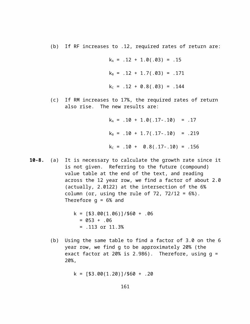
ANSWERS TO END-OF-CHAPTER QUESTIONS
12-1. An efficient market is defined as one in which the prices of securities fully reflect all known information quickly and accurately.
12-2. The three (cumulative) forms of market efficiency are:
(a) The weak form, which states that market data (price and volume information) are reflected in current prices and should be of no value in predicting future price changes.
(b) The semistrong form, which states that all publicly known and publicly available data are incorporated into stock prices.
(c) The strong form, which states that prices fully reflect all information, public and nonpublic (i.e., information that can be restricted to certain groups)
12-3. The conditions for an efficient market to exist are:
(a) A large number of profit-maximizing investors who actively participate in the market.
(b) Information that is costless and widely available to all at approximately the same time.
(c) Information that is generated in a random fashion such that announcements are basically independent of one another.
(d) Investors that react quickly and accurately to new information.
These conditions, which appear strict, are met quite closely in reality. For example, while information is not costless to produce, many market participants receive it “free” (of course, it has to be paid for in the commissions investors pay).
188
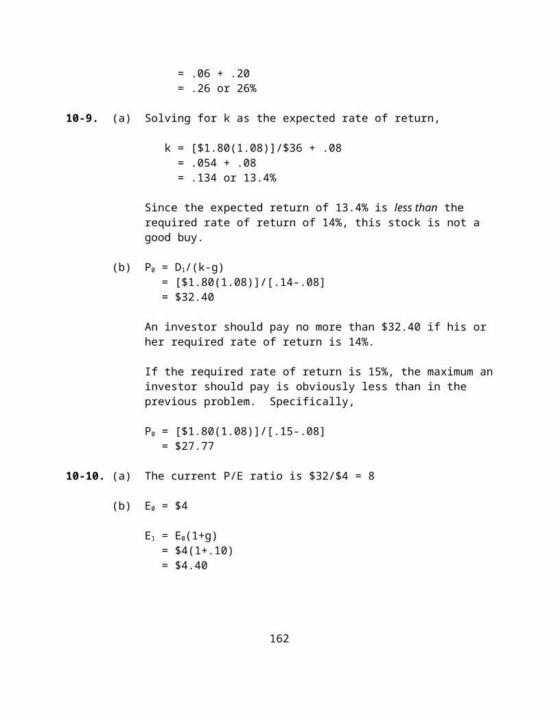
12-4. Technical analysis relies heavily on known price and volume data to predict future price changes. The weak form of the EMH states that such data should already be reflected in current prices and therefore is of no value in predicting future price changes.
12-5. Semistrong form tests are tests of the speed of price adjustments to public information. They seek to determine if investors can use publicly available information to earn excess returns.
12-6. Two different ways to test for weak form efficiency are:
(a) Statistically test the independence of stock price changes, using such techniques as the serial correlation test and the signs test.
(b) Test specific trading rules that attempt to use past price and volume data. One well-known technical trading rule is the filter rule.
12-7. Statistical significance results from formal tests in statistics, such as the calculation of the t statistic or the F statistic. Such significance relates to the probability of accepting or rejecting certain hypotheses.
Economic significance refers to the possibility of being able to actually exploit a statistical dependence. After all costs are accounted for, can excess returns be earned through such exploitation?
12-8. If the EMH is true, there are several implications for investors:
(a) Technical analysis has no validity or, at the very least, is seriously in doubt.
(b) Conventional fundamental analysis--the type done by the majority of analysts--is of little value, producing, at best, average results. What is necessary is to perform clearly superior fundamental analysis.
(c) As for money management activities, passive strategies would receive much more emphasis.
189
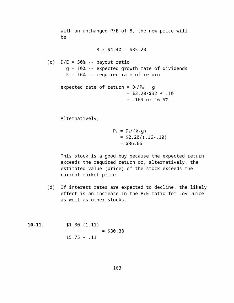
Nevertheless, several tasks must still be performed, such as diversifying, establishing and maintaining the risk level, and being concerned with the tax status of the investor and his or her transaction costs.
12-9. The performance of mutual fund investors can be a test of semistrong efficiency in the sense that the managers may be using nothing other than the publicly available information to which all investors have access. The semistrong form is concerned with publicly available information. If the managers are unable to outperform the market (after all proper adjustments) using this information, semistrong efficiency is supported.
12-10. The money management activities for a portfolio manager who believes that the market is efficient will include at least the following:
(a) ascertain that the correct amount of diversification has been achieved
(b) achieve a level of risk appropriate for the portfolio
(c) maintain the desired risk level over time
(d) be constantly aware of the tax implications of the portfolio
(e) seek to reduce transaction costs.
12-11. Market anomalies are research findings that do not support market efficiency; that is, they are evidence that inefficiencies do exist. These results are in contrast to what would be expected in a totally efficient market.
Well known anomalies include:
(a) the SUE effect, or the proposition that the adjustment of stock prices to quarterly earnings announcements occurs with a lag
190
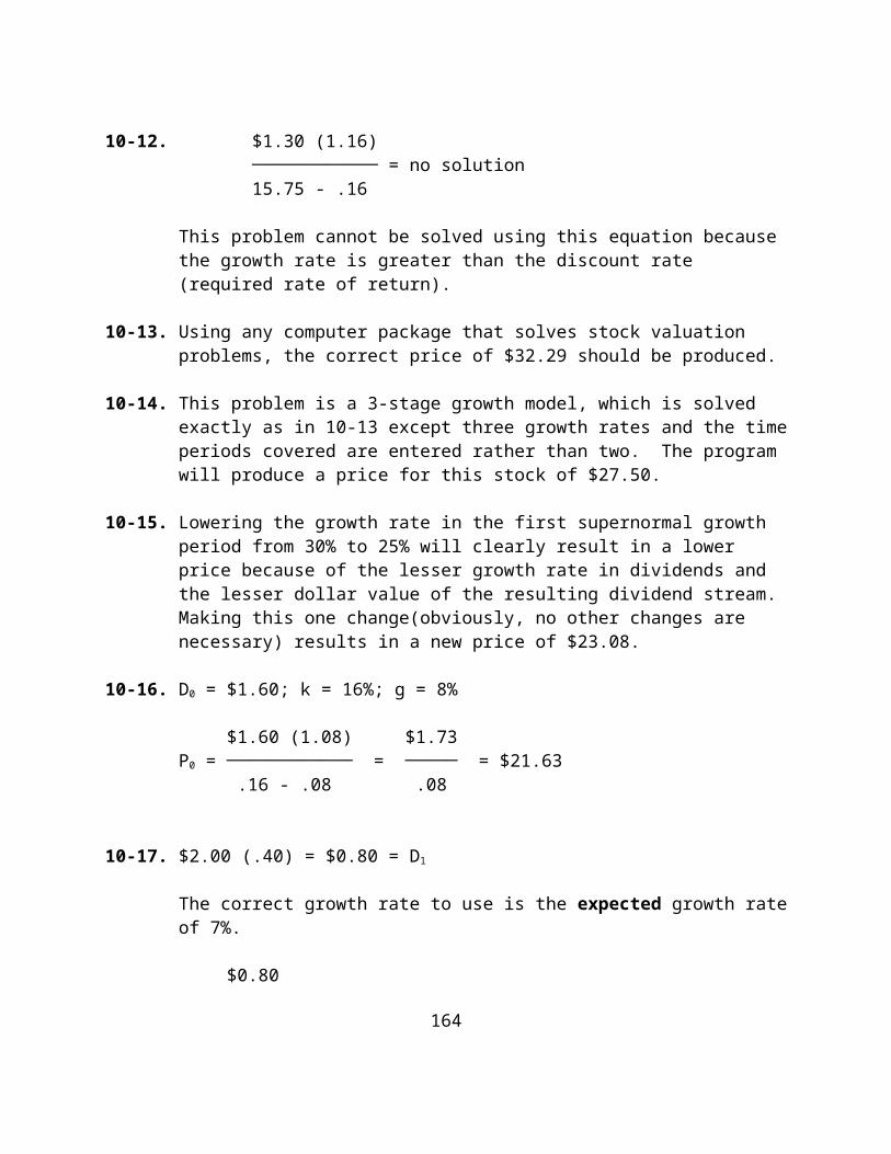
(b) the P/E effect, or the proposition that low P/E stocks will, on average, outperform high P/E stocks
(c) the size effect, or the proposition that small
capitalization stocks have earned higher risk-adjusted returns than have large capitalization stocks
(d) the seasonal effect, or the proposition that stocks have exhibited higher returns than expected in January. This could also include the monthly effect, the weekend effect, and so forth.
(e) the Value Line results, which seem to indicate that this investment advisory service has classified stocks into five groups that have performed in a monotonic fashion, with very impressive results for the top (expected best performers) two groups
12-12. If all investors believed that the market is efficient, and numerous participants ceased the pursuit and study of information about stocks, the result could be less market efficiency. Obviously, this statement would depend upon who is left to do the analysis, and how much they do. The point of this question is to stimulate thinking about what is going on in the market in the way of information gathering and processing.
12-13. SUE is directly related to fundamental analysis. First, earnings are a primary component of fundamental analysis. Second, stock prices should be expected to adjust to any unexpected information contained in the earnings, and SUE captures this unexpected element. The question is how long this adjustment takes.
12-14. Numerous types of events or information have been used in semistrong form tests. The text discusses the following: stock splits, money supply changes, accounting changes, dividend announcements, and reactions to various announcements such as major world events and the information in the “Heard in the Street” column of The Wall Street Journal.
Of course, earnings announcements have been studied in regard to semistrong efficiency. Because SUE is
191
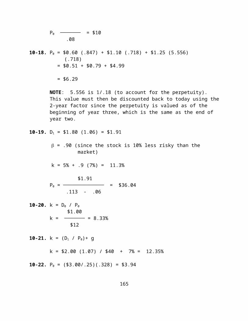
discussed in other sections of the book, it was not included in the list discussed above; however, earnings announcements are one of the major items to be studied in this regard. Furthermore, the other anomalies discussed later in the chapter, such as the P/E ratio, involve tests of semistrong efficiency.
Other studies have examined management forecasts, new issues, and options. Finally, as discussed elsewhere, tests of mutual fund performance can be regarded as semistrong efficiency tests.
12-15. In an efficient market, prices reflect information quickly and accurately. Investors could expect to buy and sell stocks at “fairly-valued” prices. Corporations could assume that when they make good decisions, or experience favorable events, the corporation’s stock price will reflect this. Funds will be better allocated in such a market. Furthermore, resources would not be devoted to pursuits of dubious or no value, such as technical analysis.
12-16. No! Upward trends are not inconsistent with weak form efficiency. Price changes can be random around an upward trend. Any random series can show clear trends.
12-17. Security analysts are still needed in an efficient market to disseminate information and value securities based on their estimates. If this were not being done, the market could become inefficient. The important question here involves the number of analysts needed to perform this role, and the type of analysis they do.
12-18. The fact that a mutual fund, or any portfolio, has outperformed the market for the last four years is not a very significant finding. To be potentially significant, we must show first of all that the results are on a risk-adjusted basis, and that all expenses relative to a buy-and-hold strategy has been accounted for. Until this is done, the statement is basically meaningless.
12-19. To conduct a fair test of a technical trading rule, certain adjustments must be made, including:
(a) risk
192
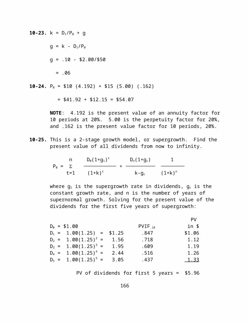
(b) transaction and other costs
(c) consistency
(d) out-of-sample validity
12-20. Filter rules are related to timing strategies, indicating when to be long or short. Filter rules should be compared with a buy-and-hold strategy.
12-21. An analysis of specialists is a test of strong form efficiency. They possess information (such as a knowledge of limit orders) not publicly available, and the issue is whether they can earn excess returns.
12-22. Some researchers writing about the size anomaly, in particular Banz and Reinganum, have attributed it to a misspecification of the CAPM. Size may be a proxy for some other variable, or may be highly correlated with other variables and be picking up part of their effects.
12-23. Directly testing the profitability of insider trading involves strong form efficiency. And tests of insider activity indicate that they do earn returns in excess of those expected.
Investors can use the insider reports that must be filed with the SEC and are, therefore, publicly available. Several advisory services report these transactions. A test of whether investors can use such publicly available information to earn excess returns is a test of semistrong efficiency.
12-24. Mutual fund data can be used to test strong form efficiency by assuming that mutual fund managers are in possession of non-public information. Since they are full-time managers with staffs to assist them, have adequate resources for research, and offer the potential for brokers to earn large commissions, it is reasonable to expect them to discover information more quickly than the average investor.
Mutual fund data can also be used to test semistrong form efficiency. If all publicly available information is
193

quickly reflected in stock prices, and mutual funds use only publicly available information, they should not be able to earn excess returns.
12-25. If the market is semistrong efficient, you would expect to see an immediate adjustment at the time the information becomes available. On a graph with stock price as the vertical axis and time as the horizontal axis, think of the price between period 0 and period 1 as a horizontal line extending from the stock price on the vertical axis.
At time period 1, the price would adjust immediately to the new (and assumed) higher price; therefore, on the graph there would be a small vertical line representing this immediate adjustment to the new and higher justified level. For completeness in this simple situation, you could then draw a new horizontal line representing the price between period 1 and period 2.
P │ r │ i │ c │ ┌───── e ├─────┘ │ │ └───────────────────────────────────────Time 0 1 2 3
If there is a lag in the adjustment of the price to this information, there would not be the sharp, immediate adjustment at period 1. Rather, this adjustment would be gradual.
12-26. The SUE analysis is not related to technical analysis, which uses market data in an attempt to forecast future price changes. SUE is part of fundamental analysis because it is concerned with the adjustment of stock prices to earnings announcements, and earnings are a primary fundamental variable.
12-27. The standard definition of an operationally efficient market is one with the lowest possible prices for
194
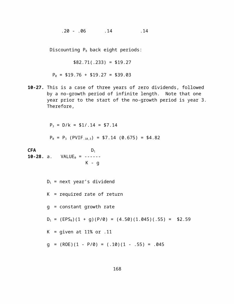
transactions services. This is different from the informational efficiency discussed in this chapter.
According to Keane, an operationally efficient market is one in which only a relatively few investors have the skill to detect a divergence between price and semistrong value. These few investors can earn economic rents. Such opportunities are not available for most investors.
CFA12-28. a.
The notion that stock prices already reflect all available information is referred to as the efficient market hypothesis (EMH). It is common to distinguish among three versions of the EMH: the weak, semi-strong, and strong forms. These versions differ by their treatment of what is meant by “all available information.”
The weak-form hypothesis asserts that stock prices already reflect all information that can be derived from studying past market trading data. Therefore, “technical analysis” and trend analysis, etc., are fruitless pursuits. Past stock prices are publicly available and virtually costless to obtain. If such data ever conveyed reliable signals about future stock performance, all investors would have learned already to exploit such signals.
The semi-strong form hypothesis states that all publicly-available information about the prospects of a firm must be reflected already in the stock’s price. Such information includes, in addition to past prices, all fundamental data on the firm, its products, its management, its finances, its earnings, etc., that can be found in public information sources.
The strong-form hypothesis states that stock prices reflect all information relevant to the firm, even including information available only to company “insiders.” This version is an extreme one. Obviously, some “insiders” do have access to pertinent information long enough for them to profit from trading on that information before the public obtains it. Indeed, such
195
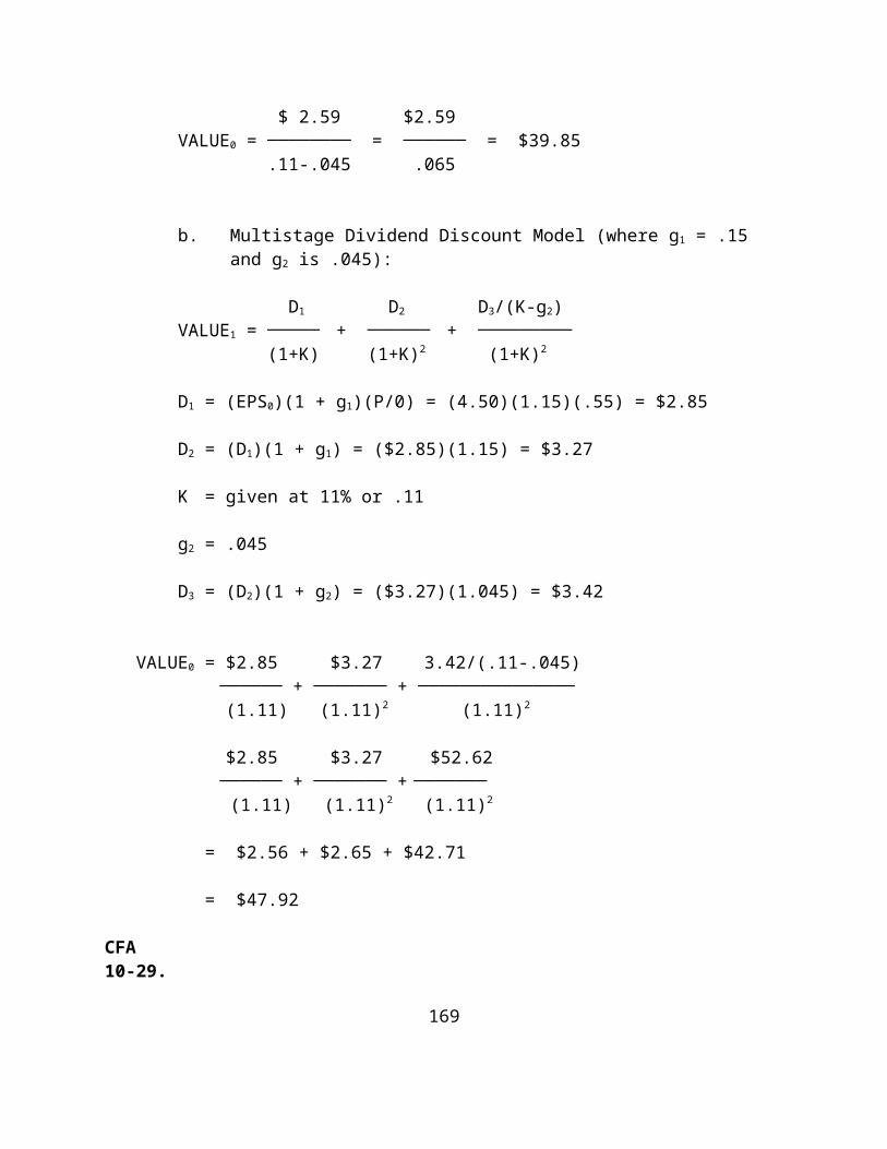
trading - not only by the “insiders” themselves, but also by relatives and/or associates - is illegal under rules of the SEC.
For the weak-form or the semi-strong forms of the hypothesis to be valid does not require the strong-form version to hold. If the strong-form version was valid, however, both the semi-strong and the weak-form versions of efficiency would also be valid.
b.
Even in an efficient market, a portfolio manager would have the important role of constructing and implementing an integrated set of steps to create and maintain appropriate combinations of investment assets. Listed below are the necessary steps in the portfolio management process:
1) Counseling the client to help the client to determine appropriate objectives and identify and evaluate constraints. The portfolio manager together with the client should specify and quantify risk tolerance, required rate of return, time horizon, taxes considerations, the form of income needs, liquidity, legal and regulatory constraints, and any unique circumstances that will impact or modify normal management procedures/goals.
2) Monitoring and evaluating capital market expectations. Relevant considerations, such as economic, social, and political conditions/expectations are factored into the decision making process in terms of the expected risk/reward relationship for the various asset categories. Different expectations may lead the portfolio manager to adjust a client’s systematic risk level even if markets are efficient.
3) The above steps are decisions derived from/implemented through portfolio policy and strategy setting. Investment policies are set and implemented through the choice of optimal combinations of financial and real assets in the marketplace - i.e., asset allocation. Under the
196
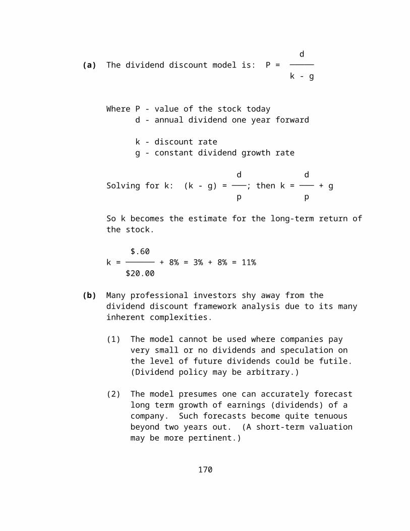
assumption of a perfectly efficient market, stocks would be priced fairly, eliminating any added value by specific security selection. It might be argued that an investment policy which stresses diversification is even more important in an efficient market contest because the elimination of specific risk becomes extremely important.
4) Market conditions, relative asset category percentages, and the investor’s circumstances are monitored.
5) Portfolio adjustments are made as a result of significant changes in any or all relevant variables.
CFA12-29. c
CFA12-30. a
CFA12-31. d
CFA12-32. d
197
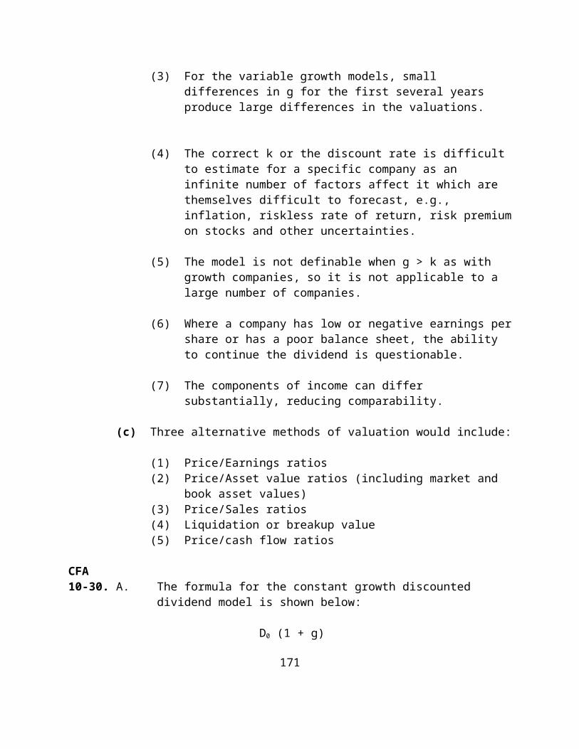
ANSWERS TO END-OF-CHAPTER PROBLEMS
12-1. SUE = (Actual Earnings - Expected Earnings) / Standard Error of Estimate
= (.50 - .30) / .05 = 4.0
This would be a good buy on the basis of the research that has been done because SUE values over 3.0 have, on average, been associated with positive excess returns, and the higher the SUE value, other things equal, the better. A SUE of 4 or better would put this stock in the top decile of SUE stocks based on previous studies.
198
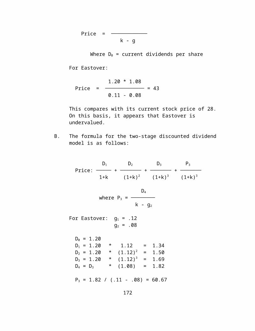
PART V SECURITY ANALYSIS
Chapter 13: Economy/Market Analysis
CHAPTER OVERVIEW
Chapter 13 is the first of four chapters explaining security analysis, and the first of three explaining the top-down approach to fundamental analysis of common stocks by proceeding from market analysis to industry analysis to company analysis. All three of these chapters stress the same model of valuation: use a discounted cash flow analysis, or, for illustrative purposes here, a P/E ratio model. In other words, estimate an expected return in the form of dividends or next year's earnings, and apply an appropriate capitalization rate or multiplier, respectively.
Chapter 13 begins by considering relationships between the economy and the stock market, with emphasis on the business cycle. It is important to emphasize that the market typically leads the economy. Macroeconomic forecasts of the economy are also considered.
The next part of the chapter focuses on understanding the stock market. It begins with an analysis of what is meant by the “market.” Given the information in Chapter 4 on market indexes, the discussion here involves the simple point that the “market” generally refers to a market index such as the Dow or the S&P 500. The remainder of this discussion focuses on the uses of market measures.
To understand the stock market, think in terms of the expected returns and risk for the market. To do this, it is instructive to examine the Keran model as presented in the text. Regardless of the fact that the Keran model was presented many years ago, it is as valid today as it was then--which should help to reassure students about the concepts being developed here.
The Keran model leads naturally to a framework of considering earnings and interest rates. One can use the framework of the constant growth version of the Dividend Discount
199
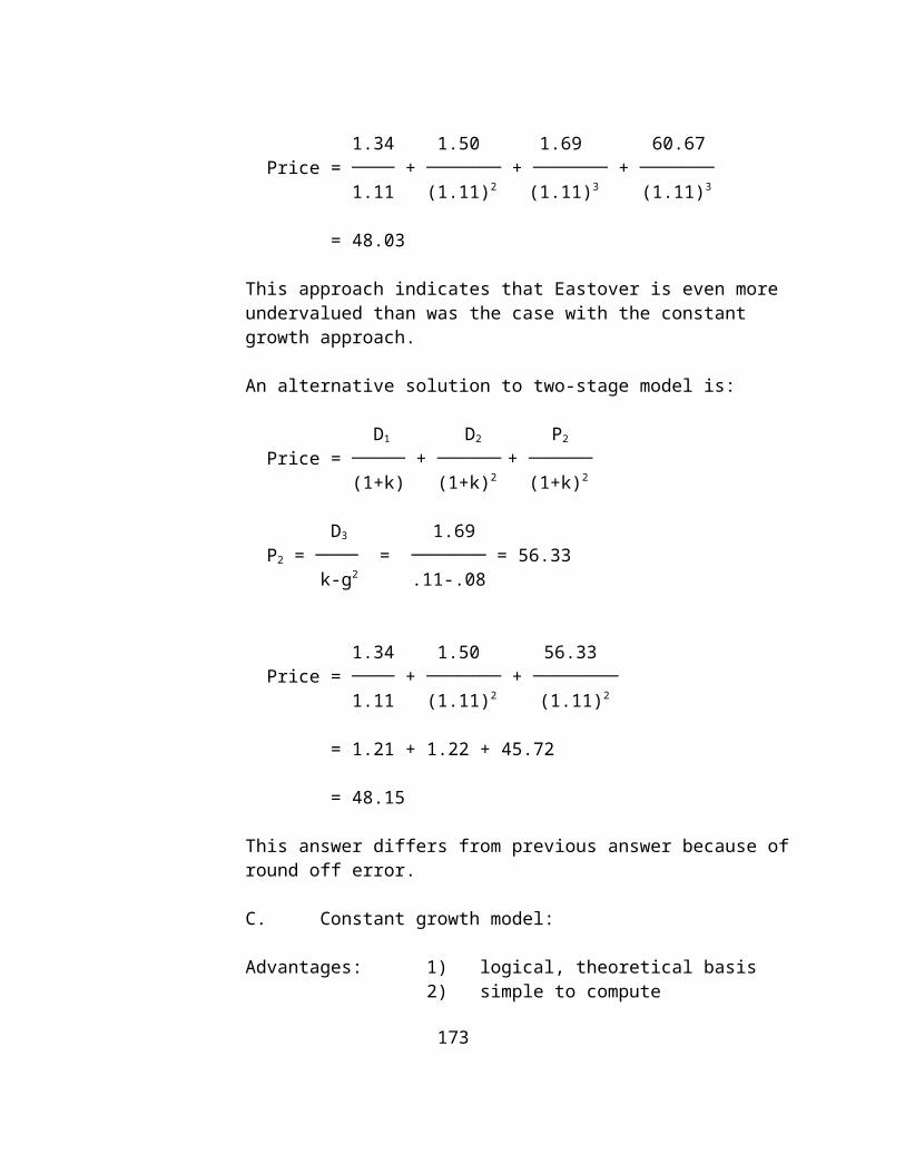
Model to illustrate the important points about what determines stock prices.
To value the market, we use the same framework and talk about estimating corporate earnings and a multiplier. Using ex post data for the market, we can examine what did happen as these variables changed from year to year. Such an exercise is useful to make students think about the logic of what is going on.
To forecast changes in the market, economic variables can be used as clues. This involves analysis of the business cycle and of such factors as monetary variables. Specific relationships between economic activity and market advances or declines have been noted, and may be useful for helping to forecast the market.
The Value Line Industrial Composite analysis is used to illustrate how various simple forecasts of the market can be made. This is useful for showing students that data are readily available for this purpose and that the underlying models themselves are simple to use. Nevertheless, errors are inevitable because we cannot forecast the future without mistakes. In the final analysis, the earnings estimate may be inaccurate, even for the year ahead, and the spread between k and g may widen or narrow. No one can possibly know for certain.
CHAPTER OBJECTIVES
To examine the relationships between the economy and the stock market.
To explain conceptually how the market can be understood and forecasts made of possible future movements in the market.
To illustrate fundamental analysis as it applies to the aggregate stock market using the same types of models developed in Chapter 10.
200
MAJOR CHAPTER HEADINGS [Contents]
Taking a Global Perspective
[the general trend worldwide is to open up economies and deregulate industries]
Assessing the Economy
The Business Cycle[basics of the business cycle; composite indexes of leading indicators; the stock market and the business cycle]
The Relationship Between the Bond Market, The Stock Market, and the Economy[bond investors react to daily information and the stock market is affected]
Forecasts of the Economy[how good are they? the impact of Greenspan]
Understanding The Stock Market
What Do We Mean by the “Market”?[most investors are referring to some market index; reasons why we need measures of the stock market]
The Determinants of Stock Prices[the Keran model of stock price determination; Corporate Earnings, Interest Rates, and Stock Prices--earnings directly related; interest rates inversely related]
Valuing the Market
[two approaches--DDM and the P/E ratio model]
The Earnings Stream[the process of estimating earnings for a market index]
The Multiplier[recent history of P/Es]
Putting the Two Together[explaining the market in hindsight]
Forecasting Changes in the Market
[the difficulty of timing the market consistently]
Using The Business Cycle To Make Market Forecasts
Using the Business Cycle to Make Market Forecasts[recognizing peaks and troughs; does January market performance forecast annual performance?]
Using Key Variables To Make Market Forecasts[the use of key indicators and macro variables]
Using Valuation Models to Make Market Forecasts[illustration of the multiplier model with Value Line data]
Appendix 13-A Published Information About The Economy-- Government Publications
POINTS TO NOTE ABOUT CHAPTER 13
Tables and Figures
Table 13-1 shows a simple analysis of interest rates and total returns on the S&P 500 Index. It clearly demonstrates the interest rate relationship with stock prices.
Figure 13-1 provides basic information by showing GDP over the last 25 years. Students should realize there is significant volatility in the series.
Figure 13-2, the Keran model of stock price determination, is useful for discussion and should be used as a transparency. It is a classic foundation for understanding the determinants of stock prices, as valid today as when it was first published.
Figure 13-3 shows an excerpt from Standard & Poor’s publication, The Outlook. It makes the point directly that stock
prices are affected primarily by earnings and interest rates, which parallels the discussion in the chapter. It is also reassuring for students to see that the points being made in the text are also being made in the popular press.
Figure 13-4 shows interest rates, corporate earnings, and the S&P 500, matched up since 1975. Recessionary periods are highlighted.
Figure 13-5 shows S&P 500 P/E ratios since 1947. It illustrates the point that P/E ratios fluctuate dramatically over time, making it very difficult to forecast the market even if an investor has a good estimate of earnings for the next period. The P/E ratio has hovered around different levels for extended periods of time, as shown in Figure 13-5. For example, in the 1960s and early 1970s it was around 17, while in the late 1970s it tended to hover around 10. In the 1990s, the P/E has been on a strong upward movement.
Figure 13-6 shows Value Line’s Industrial Composite, which is published twice annually—early in the year, and late summer. This is a convenient way to look at the overall market with data that are readily available.
This information is used in the chapter to illustrate how valuation models can be applied to forecast the market. Value Line’s analysis is quite useful for this purpose because all of the information needed is contained on one page for a market aggregate--earnings, dividends, P/E ratios, growth rates in dividends, and so forth.
Box Inserts
Box 13-1 is an interesting analysis of how investors should react during market declines, a topic of importance to most investors. The message here is to not cut and run because you will likely miss the next upturn. The real problem with market timing is deciding when to get back into the market.
The numbers and analysis presented are quite interesting, and could generate some good class discussion. Given the recent levels in the market, hitting 8000, then 9000, 10,000 and 11,000, many investors were asking should they get out of the market. Thus, instructors can use this Box Insert as the basis for
talking about a very important topic that is of interest to many investors.
ANSWERS TO END-OF-CHAPTER QUESTIONS
13-1. Market analysis is important because some 30% to 50% of the variability in an individual stock's return is attributable to aggregate market effects. Not only is the market the largest single factor explaining fluctuations in individual stock returns, it has an even greater impact on a diversified portfolio.
13-2. The two determinants of stock prices are
(a) the expected benefits stream (earnings or dividends)
(b) the required rate of return (or, alternatively, the P/E ratio).
These two determinants are equivalent to the two components of a valuation model--return and risk. Return is represented by (a), and risk by (b).
13-3. Interest rates are the basic component of discount rates, with the two usually moving together. Therefore, Keran’s model contains a proxy for the discount rate (required rate of return) used in the dividend valuation model.
13-4. The Federal Reserve directs monetary policy, which is one of the four independent variables in the Keran model. Control of the money supply through monetary policy may be quite significant in affecting such factors as output, employment, inflation, GNP, etc.
13-5. Historically, a close direct relationship has existed between corporate profits and stock prices. A parallel between the two series can often be seen, both upward and downward, although stock prices may move first.
An inverse relationship exists between stock prices and interest rates. Because interest rates are closely tied to discount rates, a rise in interest rates will have a negative impact on stock prices.
13-6. To value the market, investors need to analyze the expected earnings (or dividends) for a market index as well as an expected P/E ratio (or discount rate). These
198
values are difficult to accurately predict; however, the concept is simple and intuitive. If earnings are expected to rise and the P/E to at least remain constant, the market should rise. If a decline is expected, ceteris parabus, a drop in value can be expected. And so forth.
It is desirable for instructors to impress upon students the basic nature of this process, even if exact estimates are difficult to obtain. No one is ever going to be able to forecast the market accurately on a consistent basis, but it is possible to make some astute judgments periodically (such as in 1982 before the peak in interest rates) and benefit from them.
13-7. The primary cause of a rise in stock prices in 1982 was a dramatic decline in interest rates, and therefore discount rates. While it is not likely that many investors caught the exact bottom, a sizeable number did benefit by expecting such a decline sometime in 1982 and using this expectation in the manner suggested in the previous answer.
13-8. Stock prices tend to lead the economy's turning points, both peaks and troughs. However, there are finer points to consider:
(a) Stock prices almost always rise as the business cycle is approaching a trough. Furthermore, these increases have been large.
(b) Stock prices often drop suddenly as the business cycle enters into the initial phase of recovery. Prices stabilize, or even decline, as the economy moves ahead.
13-9. • Stocks should be purchased before a bottoming of the economy occurs because prices almost always rise before the trough.
• As the economy recovers, be prepared for a leveling off, or even a decline.
13-10. Considerable evidence suggests that investors cannot use past changes in money supply to forecast stock prices.
199
Stock price movements may lead changes in money supply. As in numerous other areas of research in investments, this relationship has been controversial, and the evidence presented has been mixed.
13-11. The market P/E is higher at the end of the slump than at its low point of the slump; in other words, the P/E ratio usually rises toward the end of each slump relative to its low point during the downturn. It then remains roughly unchanged over the next year.
13-12. The data suggest rather clearly that the P/E ratio declined over much of the 1970's. Profits, on the other hand, trended up over the last half of the decade. (Note, however, that “real” profits may have acted differently-- adjusted for inflation, inventory effects, etc. Controversy exists about the true performance of corporate profits.) Regardless, the sharp drop in P/E ratios in the mid-to-late 1970s clearly had a negative impact on the market.
13-13. You cannot answer this question with the information provided. The reason is that the value of stocks is dependent upon both components of the valuation model-- returns and risk. Therefore, while you may know with certainty what corporate earnings will do, you do not know what the discount rate (or, alternatively, the P/E ratio) will do. It could easily change more than enough to negate the favorable impact of the increase in corporate earnings.
CFA13-14. A. A basic premise of the business cycle approach to
investing is that stock prices and bond prices tend to move in cycles and those cycles tend to relate over time in a reasonably uniform way to the business cycle. For example, there is evidence that stock prices tend to move about six months ahead of the economy. In fact, stock prices are a leading indicator for the economy.
Over the course of a business cycle this approach to investing would work as follows. As the top of a business cycle is perceived to be approaching, stocks purchased should not be vulnerable to a
200

recession. When a downturn is perceived to be at hand, stock holdings should be lightened with proceeds invested in high-quality, short-term instruments which should be yielding reasonably well with a reasonably flat yield curve. Once the recession is clearly underway interest rates should be at a peak and holdings should be switched to high-quality, long-term bonds. Once the recession has matured to some extent, a switch should be made to lower quality debt instruments as yield spreads should have widened. As it’s perceived the recession is about to end, profits should be taken in the bonds and reinvested in stocks, particularly those in cyclical industries or with a high beta.
Excess returns generally will only be earned if the above switches precede these turning points by several months. Switches made after the turning points may not lead to excess returns.
B. Based on the business cycle approach to investment timing, the ideal time to invest in a cyclical stock like a passenger car company would be just before the end of a recession. If the recovery is underway, Adam’s recommendation would be late. The equities market generally anticipates the changes in the economic cycle. Therefore, since the “recovery is underway,” the price of Universal Auto should reflect the anticipated improvements in the economy.
However, since recoveries typically last for an extended period, there may still be upside left in Universal Auto's stock price as the recovery works its way through Universal Auto’s operations. Adam will want to analyze the current valuation and operating potential of Universal Auto relative to the economic recovery to determine further potential appreciation.
201
ANSWERS TO END-OF-CHAPTER PROBLEMS
13-1. NOTE: The earnings ($15.24) and dividends ($6.97) for 19X6 are given, as is the year-end price of 186.24.
a) P/E = 186.24/15.24 = 12.22D/E (100) = 100(6.97/15.24) = 45.73%D/P (100) = 100(6.97/186.24) = 3.74%
As an additional piece of information,TR = 100[(186.24-157.62+6.97)/157.62] = 22.58%
b) The indices have different base years, different base values are calculated differently, and the Value Line Industrial Index has broader coverage. The basic similarity is that they both cover industrial corporations. The price, earnings, and dividend values are not comparable. The ratios, however, may be compared.
c) k = 6.97/186.24 + .095 = .132425
d) calculated in a) above.
e) E19X7 = (1.25)(15.24) = 19.05
f) (.40)(19.05) = 7.62
7.62/19.05 .40 g) P/E = ────────────── = ─────── = 10.69
.132425 - .095 .037425
h) P = 7.62/.037425 = 203.61, or
P = 10.69(19.05) = 203.64
i) 1. P/E = .40/(.14-.095) = .40/.045 = 8.89
P = 7.62/.045 = 169.33
2. P/E = .40/(.13-.095) = .40/.035 = 11.43
P = 7.62/.035 = 217.71
202

3. P/E = .40(.12-.095) = .40/.025 = 16
P = 7.62/.025 = 304.80
203
Chapter 14: Industry Analysis
CHAPTER OVERVIEW
Chapter 14 covers industry analysis, the intermediate or second step in the fundamental analysis of common stocks which starts with market analysis and concludes with company analysis. As such, it is designed to cover the essentials of thinking about and analyzing industries without being overly technical.
The philosophy behind Chapter 14 is important to note. Beginning students in Investments are unable to do detailed fundamental analysis, both because of knowledge limitations and time constraints. The author thinks it is unrealistic to ask students to do detailed industry analysis, involving tax rates, depreciation charges, and so forth. Therefore, the emphasis in Chapter 14 is on the conceptual issues: Why do we do industry analysis, what are the problems involved, and how should we conceptually go about doing industry analysis?
In the final analysis, the point is made that industry analysis, like all aspects of fundamental analysis, comes down to estimating the future expected cash flows and discounting these cash flows at a proper discount rate, or using the estimated earnings for the industry next year and an appropriate P/E ratio. It is more important to get students to think about the conceptual issues involved in doing security analysis than in too many details of industry analysis that most will not understand or use again.
Chapter 14 first documents the importance of industry analysis by showing how some industries outperform others over various time periods. There is no doubt that some industries outperform others over long periods of time. The discussion next demonstrates that short-term consistency is very difficult to find, which means that we cannot simply buy the industries that performed well last year and expect them to perform well this year. In many cases the opposite is true--bad performers for one year become good performers in the next year or the year after that. Therefore, investors interested in both long-term
204
performance and shorter-term performance must do industry analysis.
Chapter 14 also examines such issues as the definition of industries and the problem with classifying a particular company in one industry. The industry life cycle, which is often used as part of industry analysis, is explained as a conceptual method of analyzing industries. The implications of business cycle analysis for industries are considered, which provides useful classifications for industries such as growth industries, defensive industries, cyclical industries, and interest-sensitive industries.
Qualitative aspects of industry analysis are presented, including brief excerpts from the well-known Porter material on industry analysis. Two well-known diagrams from the Porter analysis on industries, one showing the five competitive forces that determine industry profitability and one showing the elements of industry structure, are included in the discussion. Once again, this analysis is consistent with the approach emphasized on the CFA examinations, particularly at Level II.
The sources of industry information are covered in an appendix, consistent with the philosophy of having descriptive material such as this in an appendix.
CHAPTER OBJECTIVES
To demonstrate why industry analysis is an important component of fundamental analysis, and why we must do industry analysis.
To explain conceptually how to analyze industries. The emphasis is on the broad conceptual approach, and not the specific details which cannot readily be mastered by beginners.
To discuss various aspects involved in industry analysis. A central focus of this material is some excerpts from the Porter analysis.
205
MAJOR CHAPTER HEADINGS [Contents]
Performance of Industries over Time
The Importance of Industry Analysis Over Long Periods[comparisons of industry price indices over various periods]
Consistency of Industry Performance[consecutive-year performance comparisons show instability]
What Is an Industry?
[problems in determining what industry a company is in]
Classifying Industries[SIC system, other classifications such as Value Line]
Analyzing Industries
The Industry Life Cycle[pioneering; expansion; stabilization; implications for investors]
Qualitative Aspects of Industry Analysis[historical; competition; government; structural changes; the Porter analysis--five competitive forces and elements of industry structure]
Evaluating Future Industry Prospects
[brief verbal explanation of how to do this]
Assessing Longer-Term Prospects
Picking Industries for Next Year[some empirical findings]
Business Cycle Analysis[growth industries; defensive industries; cyclical industries; interest-sensitive industries]

Appendix 14-A Sources of Industry Information
[general information--S&P, Forbes, etc.; specific information]
POINTS TO NOTE ABOUT CHAPTER 14
Tables and Figures
Table 14-1 is useful for discussion purposes about the performance of various industries over time and the consistency of performance over short periods. This table illustrates the large differences that occur in industry performance over time, both over long periods and over shorter periods.
Two points should be emphasized. It clearly matters which industries an investor buys into over long periods of time because some industries are going to perform very well, and some very poorly. A second important issue is whether future performance can be predicted from past performance. The evidence presented here suggests that while some continuation occurs, it is not readily apparent that the future strong performers can be predicted from past performance. This should come as no surprise in investing.
Figure 14-1 illustrates the industry life cycle. This is a simple but well-known part of industry analysis which does provide some valuable insights.
Figure 14-1 shows Porter’s five competitive forces that determine industry profitability. This discussion is based on well-known work by Porter on the issue of competitive strategy, which involves the search for a competitive position in an industry.
Figure 14-2 is a follow-up to Porter’s work. While the five competitive forces determine industry profitability, the strength of each of these factors is a function of industry structure. Exhibit 14-2 shows the important elements of industry structure.
Box Inserts
Box 14-1 is an interesting discussion of a technique suggested by S&P in its publication, The Outlook. It indicates that picking industries on the basis of their prior year's performance relative to the S&P 500 Index can produce superior results. What is interesting about this is that both last year’s leaders and last year’s laggards are recommended, as long as they are exhibiting upward momentum.

ANSWERS TO END-OF-CHAPTER QUESTIONS
14-1. It is difficult to classify industries because of the problem of determining in which industries particular companies belong. Companies often cross traditional industry lines. Industries continue to become more mixed in their activities and less identifiable with one product or service. At best, industries cannot be identified casually.
14-2. Industry analysis is valuable because industries have turned in widely-varying performances in the past, and undoubtedly will continue to do so in the future. Investors’ results have been greatly affected by the industries in which they invested. Some industries’ price performance have been virtually flat over long periods, while others show very large gains.
14-3. Obviously, differences of opinion will exist about industries expected to perform well in the future. In the next five years (i.e., roughly 2000-20005), such industries as information/communications and medical technology (artificial organs, genetic engineering, etc.) may do well. Over the next 10 to 15 years, instructors and students are free to make their own choices.
14-4. Year-to-year industry performance is not consistent. Investors cannot simply choose industries performing well in the recent past and expect this to continue over the next several years.
14-5. The stages of the industry life cycle are the pioneering stage, the expansion stage, and the stabilization stage. It is also possible to talk of a fourth stage--decline, either on an absolute or a relative basis.
14-6. The internet-related activities, such as E-commerce, is in the pioneering stage. The medical service industry is in the expansion stage as is cellular phones. The supermarket industry is in the stabilization stage, as is the electric utility industry. Declining industries could include, as possibilities, steel and metals and mining.
210
14-7. The pioneering stage offers the greatest risk.
14-8. Cyclical industries, such as autos, appliances, and houses, are the most sensitive to the business cycle. Defensive industries, such as the food industry, are the least affected by recessions and economic adversity.
14-9. Investors should analyze the stage of the business cycle and the likely movements in interest rates. As the economy approaches a recession, cyclical industries are likely to be more affected than other industries while defensive industries will be least affected. An expected rise in interest rates will have adverse consequences for such industries as homebuilding and savings and loans.
14-10. The fundamental valuation of industries is based on the same concept of valuation used throughout the book. Specifically, it is necessary to estimate the expected returns (earnings or dividends) and a multiplier (or, alternatively, a discount rate) for industries, as was done in the preceding chapter with the market, or as will be done in the next chapter with individual companies.
14-11. Several sources of information would be useful to an investor doing a detailed industry analysis.
• Standard & Poor’s Industry Survey provides basic data.
• Dun & Bradstreet Key Business Ratios provides ratio information.
• The Quarterly Financial Report for Manufacturing, Mining, and Trade Corporations, a government publication, provides timely information on individual industries.
• Forbes magazine rates industry performance annually in its January issue. This gives investors calculated information for a five year period.
• The Media General Financial Weekly publishes up-to-date weekly information on about 60 industries, showing recent price performance.
• The Value Line Investment Survey estimates industry statistics for both the current year and the coming year, and ranks all industries covered in terms of timeliness (probable performance over the next 12 months).
211
14-12. Figure 14-A1 (from Value Line) shows the industries covered by Value Line (typically, between 90 and 100) ranked in order of timeliness--probable performance over the next 12 months. Investors should pay attention to those industries ranked at the top in searching for stocks to buy. This does not mean that other stocks are not good buys, but that stocks in the top-ranked industries are likely to perform better. Investors should consider avoiding stocks in the industries ranked at the bottom in terms of near-term performance. On the other hand, some stocks in these industries are probable turnaround situations.
CFA14-13. Note: Candidates could select any three of the following
five competitive forces and then relate those selected to both Ford and Merck.
1. Rivalry among existing firms.
a) Ford faces intense competition from other domestic and foreign auto manufacturers.
b) Merck has a dominant market share in many of its product lines because a limited number of companies can supply specific drugs. For many of its most profitable drugs, Merck faces no competition for an extended period of time because of patent protection. Hence, Merck's dominant market share and limited competition allow it to develop strategies of product differentiation and focusing on market segments.
2. Threat of new entrants.
a) Despite substantial capital requirements and technological barriers to entry, domestic auto manufacturers have seen foreign manufacturers establish strong market positions.
b) The drug industry has natural barriers to entry as years of research are required to develop competing products and receive FDA approval to
212
market. Once patent protection has been achieved, Merck can take advantage of product differentiation and focus on market segments.
3. Threat of substitute products.
a) A Lexus can be substituted for a Lincoln and a Chevy for a Ford. In addition, some buyers can substitute other products such as motorcycles for cars.
b) Some drugs provide unique therapy while others have limited prescription substitutability. Again, Merck can focus on market segments and differentiate its products.
4. Power of buyers.
a) A car buyer has several alternatives among different brands and modes of transportation. In addition, the potential buyer can defer purchase by repairing an older car. Accordingly, manufacturers are often forced toprovide rebates to stimulate sales, cutting profit margins.
b) Drugs, on the other hand, are aimed at specific ailments, and potential purchasers are unlikely to defer purchase once the drug has been prescribed by a doctor. Frequently, insurance companies or the government picks up the cost of the prescription. Accordingly, drug companies have a great ability to increase prices with little consumer resistance. Again, Merck can focus on market segments.
5. Power of suppliers.
a) In theory, Ford should have an advantage here because auto manufacturers exercise great control over their suppliers. Some of these suppliers have Ford as their major customer. This could be important in cost containment. However, there are no hints in the financial
213
statements that Ford has been able to exploit its power over suppliers in recent years.
b) Merck has no special advantages in dealing with its suppliers.
CFA14-14. A. The concept of an industrial life cycle refers to
the tendency of most industries to go through various stages of growth somewhat resembling those of a person. Generally four stages are talked about with no uniformity in the length of each stage. The rate of growth, the competitive environment, profit margins and pricing strategies tend to shift as an industry moves from one stage to the next although it is usually difficult to pinpoint exactly when one stage has ended and the next has begun.
The initial stage is characterized by perceptions of a large market and by a high optimism for potential profits. Little or no profits are usually achieved, however, in this stage and there is usually a high rate of failures. In the second stage, often called rapid expansion or follow-through, growth is high and accelerating, the markets are broadening, unit costs are declining and quality is improving. The third stage, usually called mature growth, is characterized by decelerating growth caused by such things as maturing markets and/or competitive inroads by other products. Finally, an industry reaches a stage of full maturity in which growth slows or even declines.
Product pricing, profitability and industry competitive structure often (though not necessarily) vary by phase. Thus, for example, the first phase usually encompasses high product prices, high costs (R&D, marketing, etc.) and a (temporary) monopolistic industry structure. In phase two (rapid expansion), new entrants appear and costs fall rapidly due to the experience curve. Prices generally don't fall as rapidly allowing profit margins to increase. In phase three (mature growth), growth begins to slow as the product or service begins to saturate the market, and
214
significant price reductions become less common. There’s a choking out of competitors as quality and other non-price factors become more important as competitive tools. In the final stage, industry cumulative production is so high that production costs have stopped declining, profit margins are thin (assuming competition exists), and the fate of the industry depends on the extent of replacement demand and the existence of substitute products/services.
B. The passenger car business in the United States has probably entered the final stage in the industrial life cycle because normalized growth is quite low. The information processing business, on the other hand, is undoubtedly earlier in the cycle. Depending on whether or not growth is still accelerating or not, it is either in the second or third stage.
C. Cars: In the final phases of the life cycle, demand tends to be price elastic. Thus, Universal can't raise prices without losing volume. Moreover, given the industry’s maturity, cost structures are likely to be similar across all competitors, and any price cuts are likely to be matched immediately. Thus, Universal’s car business is boxed-in--product pricing is determined by the market--the company is a “price-taker.”
Idata: Idata should have much more pricing flexibility given its phase in the industrial life cycle. Demand is growing faster than supply, and, depending on the presence and/or actions of an industry leader (umbrella or experience curve pricing), Idata may price high to maximize current profits and generate cash for product development or price low in an effort to gain market share.
215
Chapter 15: Company Analysis
CHAPTER OVERVIEW
Chapter 15 concludes the three chapter sequence on fundamental security analysis by discussing the analysis of individual companies. It expands on the discussion in Chapter 10 involving valuation methods by examining more closely the components involved when implementing either the Dividend Discount Model or the P/E ratio model.
216
Starting with a discussion of what fundamental analysis is, the chapter devotes considerable space to understanding earnings, one of the two components of the multiplier valuation model. This is done by examining the financial statements for Coca-Cola, and analyzing the determinants of accounting EPS.
Ratio analysis is used to show how the firm's variables interact in determining EPS, with particular emphasis on ROE and its determinants. It is important to note here that the analysis of the financial statements, involving the calculation of ROA and ROE, follows the format used on the Level I CFA examination. This allows the use of CFA examination questions to illustrate these points, and shows students that what they are learning here exactly parallels the type of knowledge they are expected to have when seeking a CFA designation, which is widely recognized in the money management business.
A thorough discussion is included of which earnings are important (future earnings), and how one might go about forecasting earnings and earnings growth. Both security analysts’ estimates and mechanical estimates are examined. The concept of unexpected earnings is explained and illustrated. Chapter 15 contains an up-to-date discussion of the earnings “process,” including whispers, consensus estimates, the management of earnings, and more.
The remainder of the chapter is devoted to the P/E ratio, the other half of the valuation equation when using a multiplier model. Each of the three determinants of the P/E ratio are examined in detail. Coke’s P/E is examined, and the reasons why P/Es vary from company to company are discussed. Additional company analysis, including the beta, is considered.
Chapter 15 will help students to better understand the components of a valuation model--what they are, why they are being used, how they are determined, and so forth. In Chapter 10 students learn to calculate intrinsic values for stocks but do not have the opportunity to go behind the calculations. This chapter provides that opportunity.
When covering Chapter 15, it is strongly recommended that instructors emphasize such daily issues as earnings surprises, which drive stock price changes to a significant extent. There are plenty of examples available in the press each day on
217
earnings surprises, and from major websites such as CBS.Marketwatch and Yahoo!Finance.
The text strongly argues that fundamental security analysis should be performed in a particular order, and that means company analysis is the last step. On the other hand, by the time students get to Chapter 15 they should have a good feel for the subject matter and be able to really start understanding conceptually what fundamental security analysis is all about which is all one can expect at this point.
CHAPTER OBJECTIVES
To explain fundamental security analysis at the company level.
To examine the details behind the valuation models used in Chapter 10.
To use approaches for analyzing earnings that are comparable to those used on CFA examinations, thereby allowing actual CFA examination questions to be used as part of the problem set.
To stress the importance of both understanding and making forecasts of EPS and P/E ratios.
218
MAJOR CHAPTER HEADINGS [Contents]
Fundamental Analysis
[two alternative ways of calculating intrinsic value: the dividend discount model and the P/E ratio model; the importance of earnings as shown by a close relationship between change in earnings per share and change in stock price]
The Accounting Aspects Of Earnings
[the importance of EPS]
The Financial Statements[the balance sheet and income statement; illustrations of both using Coca-Cola's financial statements; certifying the statements on the basis of GAAPs]
The Problem with Reported Earnings[how different accounting methods can produce varying EPS; the FASB; the role of accountants and management; the concept of earnings quality]
Analyzing A Company's Profitability
[EPS, ROE, ROA, and leverage based on ratio analysis; the accounting definition of EPS]
Analyzing Return on Equity (ROE)[definition of Return on Assets (ROA); the four ratios that comprise ROA, with an example for Coca-Cola; the effects of leverage; how leverage and ROA go together to determine ROE; ROE calculated using five ratios, with example for Coca-Cola]
Estimating the Sustainable (Internal) Growth Rate[definition and analysis of g, the internal or sustainable growth rate]
Earnings Estimates
[involves the future earnings, not the past]
A Forecast of EPS[security analysts' estimates; mechanical estimates]
The Accuracy of Earnings Forecasts[evidence on analysts vs. mechanical estimates]
Earnings Surprises[unexpected earnings or earnings surprises; SUEs; the earnings “game”]
Useful Information for Investors About Earnings Estimates[summarizes the discussion about earnings forecasts]
Sales Growth—An Alternative to Earnings[examines the newer emphasis on sales growth]
The P/E Ratio
Determinants of the P/E Ratio[discussion of each of the three components: payout; required rate of return; expected growth rate; analyzing the P/E ratio]
Why P/E Ratios Vary Among Companies[expectations about future growth rates; variability in P/Es; illustration of P/Es from Value Line]
Fundamental Security Analysis In Practice
[the beta coefficient; relationships expected on average; a page from The Value Line Investment Survey]
Appendix 15-A Sources of Information For Common Stocks
The Financial Press (Newspapers; Magazines) Corporate Reports Brokerage Firms Investment Information Services Investment Advisory Services and Investment Newsletters (Value
Line; Other Advisory Services and Letters)
POINTS TO NOTE ABOUT CHAPTER 15
Tables and Figures
Exhibits 15-1 and 15-2 show the balance sheet and income statement respectively for Coke to facilitate the discussion of accounting data as it is needed for security analysis. Only a very basic and brief review of accounting terms is included here.
Exhibit 15-3 is new to the 8th edition. It shows the Statement of Cash Flows for Coke in order that this important variable can be discussed.
These financial statements can easily be replaced by those for other companies or bypassed if it is felt the student does not need this review. Thus, instructors have considerable flexibility in using this material.
Exhibit 15-4 shows weekly ratings of the highest and lowest P/E stocks by The Value Line Investment Survey. Students can see the wide range of P/E ratios, and instructors may wish to expand on why such a wide range exists at any point.
Exhibit 15-5 shows a typical company coverage (in this case, Coca-Cola) from The Value Line Investment Survey. This is useful both to illustrate the analysis of Coke as is done in this chapter and to show students what is available and widely used when doing security analysis. The use of this figure in Chapter 15 is in keeping with the theme of the seventh edition of using material where it is needed, rather that simply presenting it in a separate chapter as a source of information.
Figure 15-1 shows the relationship between earnings changes and price changes, and is well worth emphasizing as a transparency. Perhaps it makes the case as well as anyone is likely to see it, but it is clearly dramatic and hammers the point home extremely well. It is highly recommended as a basis
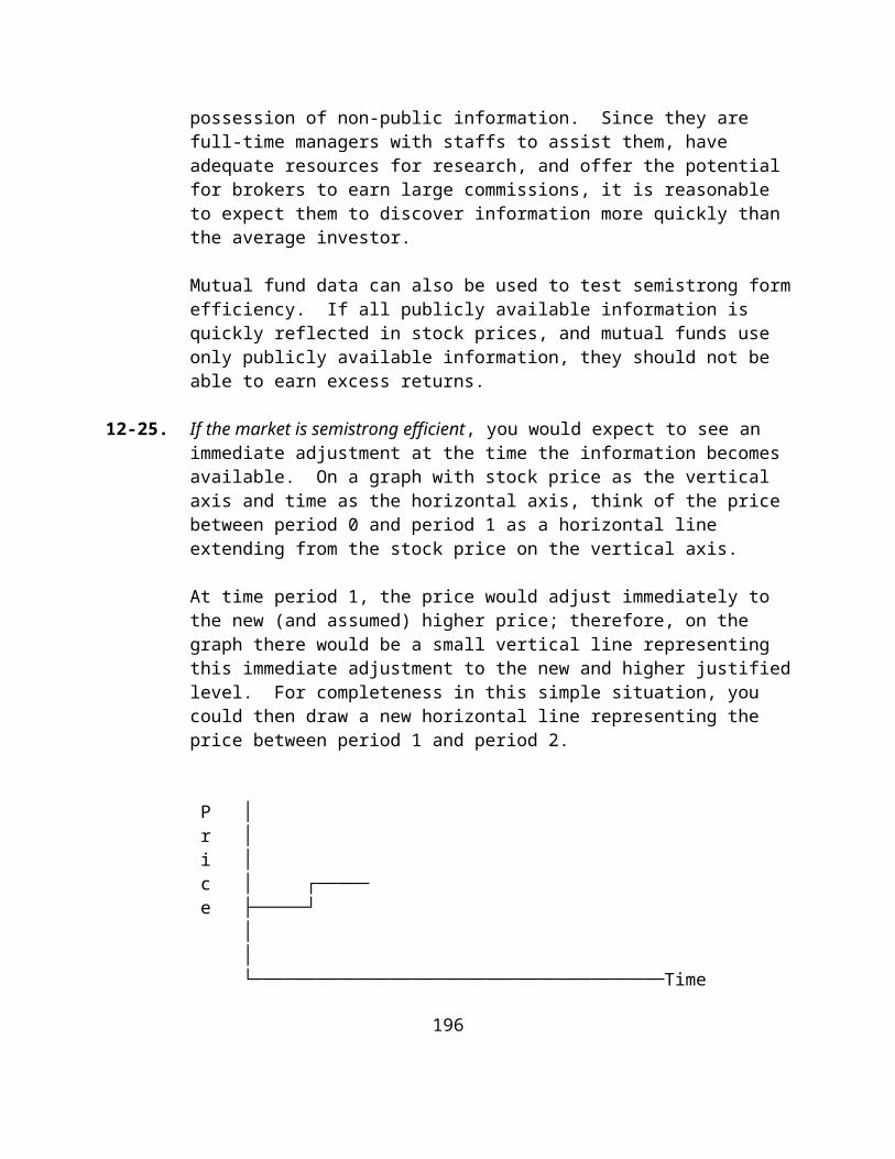
for class discussion and to emphasize the point--earnings changes and stock price changes are closely related.
Box Inserts
Box 15-1 is an interesting discussion, from the popular press, of a new emphasis in security analysis—focusing on sales growth. Some believe more companies are now trading on revenue growth rather than earnings growth.
Box 15-2 is a straightforward description of P/E ratios as carried in the popular press. It has a very complete description of the issue, and it is good for students to see its emphasis in the popular press.
Box 15-3 is a good example of security analysis, with one person saying to buy HandSpring and one saying don't buy. This is what investing is all about, differences of opinion. This type of exhibit gives instructors a good opportunity to emphasize how investors differ on the future prospects of companies, which in turn makes trading in the markets viable.
ANSWERS TO END-OF-CHAPTER QUESTIONS
15-1. In fundamental analysis, the intrinsic value of a stock is its justified price; that is, it is the price justified by investors' evaluations of a company's fundamental financial variables.
15-2. A stock’s intrinsic value can be estimated by using the dividend discount model or the earnings multiplier model.
15-3. The limitations of using the normal (constant) growth version of the dividend valuation model are:
(a) The model is only applicable if dividends can be expected to grow at a constant rate (at least approximately) over the future.
(b) It is necessary to estimate g, the expected growth rate in dividends. Obviously, different users of the model will (legitimately) come up with different estimates of the future growth rate, and it is impossible to determine ex ante who is correct.
(c) k, the investor’s required rate of return, must be estimated, an imprecise process.
15-4. “GAAP” refers to Generally Accepted Accounting Principles, a standard set of rules developed by the accounting profession primarily on the basis of historical costs. These principles assure some uniformity in the financial statements produced by companies.
15-5. The problem with accounting earnings is that alternative accounting principles can be used to prepare financial statements. Numerous combinations of these principles are possible. It is probably impossible to estimate the true performance of a company in one accounting figure.
15-6. The auditor’s report signifies only that generally accepted accounting principles were applied on a consistent basis. It does not guarantee the accuracy or the quality of the earnings in an absolute sense.
15-7. The management of a company hires an auditing firm to prepare the financial statements. The accounting firm is supposed to conform to accepted accounting standards and act independently. However, management may be able to influence the accounting firm, which wishes to keep the business, because some flexibility in how certain items are treated does exist.
15-8. The concept of earnings quality has to do with the qualitative (and subjective) factors that contribute to producing the earnings figure and that help to assess the true earning power of the company. There are no absolute elements of earnings quality, but some guidelines for determining quality involve: liberal versus conservative accounting policies, the integrity of the reporting period, the use (or misuse) of discretionary costs, the variability of earnings, and balance sheet analysis.
15-9. The determination process for earnings:
• EPS is the product of ROE (return on equity) and book value per share.
• ROE is the product of ROA (return on assets) and leverage (total assets divided by equity).
• ROA, in turn, is the product of the net income margin and turnover.
15-10. A firm has two basic choices in financing, debt and equity. Debt is a cheaper source of financing, but it is more risky because of the fixed interest payments which must be made. If leverage is favorable, it can magnify the EPS (or diminish them if unfavorable). Given the ROA, leverage determines the ROE, one of the two basic components of EPS.
15-11. Although higher ROE leads to higher EPS, two factors determine stock price, the ultimate variable of interest to investors. The increasing use of debt financing increases the risk to stockholders, raising their required rate of return. The increase in the required rate of return will, at some point, offset the higher EPS and lower the stock price.
15-12. The earnings growth rate, g, is defined as:
g = br
where r = ROE and b is the retention rate (1 - dividend payout ratio). This is an important formulation in fundamental analysis.
15-13. Earnings growth rates for individual companies usually do not persist over time. Investors cannot simply assume that a particular trend will continue. Year-to-year growth rates are often quite variable.
15-14. Investors can obtain the forecasts of security analysts from several sources such as The Value Line Investment Survey and other investment advisory publications, brokerage houses, and data banks accessible through a personal computer. Alternatively, mechanical estimates can be made, using procedures such as time series models. The evidence is mixed as to which source is better. Brown and Rozeff found that analysts’ (specifically, Value Line) estimates were superior. However, there is no real consensus on this issue.
15-15. Malkiel and Cragg, among others, have shown how important it is to know what the market thinks the earnings growth rate will be. Investors form expectations about EPS, and these expectations play a key role in affecting stock prices. In short, earnings expectations are a key variable in selecting stocks.
15-16. The unexpected component of EPS consists of the earnings surprise factor. One way to use this factor is by calculating a stock’s SUE, the ratio of the unexpected earnings to a standardization value. Having calculated SUEs for a group of stocks, those ranking at the top (i.e., the highest SUE stocks) are selected for purchase. Those with the lowest SUEs are candidates to be sold if owned, or possibly sold short.
15-17. SUE is closely related to fundamental security analysis. Earnings is one of the primary variables in fundamental analysis. Earnings surprises should be, and are, closely related to changes in stock prices. Unexpected information about earnings justifies a revision in investor probability beliefs about the future and, therefore, an adjustment in stock prices.
15-18. P/E ratios are often shown on a current basis (current stock price divided by the latest 12 months earnings per share). Alternatively, the P/E could be calculated using the estimated earnings for the next period (typically, a year).
15-19. Any P/E ratios collected will reflect the specific time periods.
The purpose of this exercise is twofold:
(a) To show students the differences in P/E ratios among companies at a given time--in this case, the average annual P/E ratios for a year. For example, investors were willing to pay over 26 times earnings for EG&G but only 16 times for Apple Computer in one particular year. It is easy to generate discussion about the potential return and risk involved in owning these companies, which are quite different types of companies, by comparing numbers such as these. Instructors should point out that certain types of companies--for example, financial institutions, typically have low P/E ratios.
(b) To show the differences in P/E ratios across time for all companies, but in particular high technology and growth companies. Coke’s P/E ratio has varied greatly over the years. Apple Computer was relatively stable for a company in the volatile computer industry, but by 1997 Apple had run into severe problems and was facing the issue of survival. Electric utilities can be expected to show low, but relatively stable, P/E ratios.
15-20. As Equation 15-9 shows, the three variables that affect the P/E ratio are:
(a) The dividend payout ratio (direct relation)
(b) The required rate of return (inverse relation)
(c) The expected growth rate in dividends (direct relation).
15-21. (a) Earnings and dividends are directly related; therefore, an increase in the expected growth rate of earnings would equate with an increase in g, which is directly related to the P/E (the typical assumption is that the payout ratio is constant; therefore, g is the expected growth rate in both dividends and earnings).
(b) A decline in the expected payout will lead to a decline in the P/E.
(c) An increase in the risk-free rate of return will result in a rise in k and, therefore, a decline in the P/E.
(d) An increase in the risk premium will result in a rise in k and, therefore, a decline in the P/E.
(e) A decrease in the required rate of return will increase the P/E.
15-22. Beta reflects the relative systematic risk for a stock. Other things being equal, the higher the beta, the higher the risk, and the higher the required rate of return. Investors will want to know about a stock’s beta in order to estimate the volatility of the stock’s returns. If a rise in the market is expected, investors would prefer, other things being equal, stocks with higher betas. Likewise, with an expected market decline, lower betas would be preferred if stocks are to be held.
15-23. Beta is not the only component of a stock’s return. Return is a function of two components, the systematic component (which includes the beta) and the unique component (that part attributable to the company itself). This analysis is based on the market model.
15-24. Obviously, the exact answer to this question will depend upon the Value Line issue used. However, it is to be expected that the P/Es will show some significant differences, and as the timespan increases these differences will become more pronounced. In short, the P/E ratio is not likely to be stable over time.
ANSWERS TO END-OF-CHAPTER PROBLEMS
15-1. For 19X5, the calculations for parts (a), (b) and (c) are:
(a) 100(721/8256) = 8.73%(b) 100(289/8256) = 3.50%(c) 289/51.92 = $5.57
The same values for 19X1-19X4 are:
Year (a) (b) (c) 19X1 9.6% 4.2% $4.65 19X2 9.0 4.3 5.12 19X3 8.6 3.9 5.16 19X4 8.3 2.6 4.47
(d), (e), (f), (g), and (h) are calculated for 19X5, and are summarized for 19X1-19X5 below.
(d) 2315/1342 = 1.72(e) (736/2804)(100) = 26.2%, as a percentage(f) 1872/51.92 = $36.06(g) 100 (Net Income after tax/Common Equity) =
100(289/1872) = 15.4%(h) (289/4310)100 = 6.7%
Year (d) (e) (f) (g) (h)
19X1 2.05 14.9% $26.46 17.6% 9.0%19X2 1.86 13.8 29.62 17.3 8.619X3 2.11 18.4 32.57 15.8 8.219X4 1.86 29.3 32.88 13.6 5.7
Again the 19X5 calculations will be shown for (i) - (n), and summarized for the other years.
(i) 4310/1872 = 2.30 NOTE: 2.30 X 6.7% = 15.4%, the ROE(j) (289/8256)100 = 3.5%, as a percentage(k) 8256/4310 = 1.92(l) 535 + 139 = $674 mn.(m) (289/674)100 = 42.9%(n) (674/8256)100 = 8.2%
234
Year (i) (j) (k) (l) (m) (n)
19X1 1.94 4.2% 2.13 $483mn 48.0% 8.8%19X2 2.01 4.3 2.00 509 50.3 8.519X3 1.93 3.9 2.13 523 48.8 7.919X4 2.37 2.6 2.16 570 38.8 6.8
(o) Evaluate the current status of the health of GF: Examining the figures for the years 19X1-19X5 from parts (a) to (n), we see that ROE declined through 19X4, although it recovered somewhat in 19X5. The same is true of ROA. Leverage has increased. Operating efficiency declined through 19X4 before turning up in 19X5.
Reviewing more basic components, we see that operating income/net revenue has been deteriorating, as has net profits/revenue. The current ratio has deteriorated.
In summary, it would appear that GF underwent some deterioration between 19X1 and 19X5, with some (but not complete) improvement in 19X5. Examining the ROE and ROA in 19X5, we can see that GF had recovered some ground, but still compared unfavorably to 19X1 and 19X2.
15-2. (a)Year 100(D/E)% ROE% TR%
19X4 49.2% 14.5% 16.319X5 40.1 18.9 29.619X6 35.5 16.9 23.7
(b) for dividends: (1+r) = 2.40/1.72 = 1.3953491/5 = 1.068899, r% = 6.9%
It is assumed that measurement begins at the beginning of 19X2; therefore, we use the year-end 19X1 number.
for earnings: (1+r) = 6.75/4.56 = 1.4802631/5 = 1.081603, r% = 8.2%
235
(c) P/E = $47/$6.75 = 6.963
(d) (7)($7.50) = $52.50
(e) Coca-Cola is a blue-chip company but with a very good growth record. GF is a stable, blue chip company in a pedestrian line of activity with dividends growing approximately in line with the economy as a whole. Earnings growth for Coca-Cola has been much more rapid than for GF. Therefore, Coca-Cola would have commanded a larger P/E than GF in the past.
(f) .4/(.14-.07) = .4/.5 = 8
(g) r = 1-.4 = .6; g = .6(.15) = .09
CFA15-3. A. Decomposition of ROE or duPont System:
1990 Components
Tax Burden = Net Income/pretax income
= $1650/$2550= .647
Interest Burden = Pretax Income/Pretax Income + interest expense
Operating Margin = Pretax Income + interest expense/Sales Revenue
= $2550 + $10/$7120= .36
Asset Turnover = Sales Revenue/Total Assets
= $7120/$7250= .982
236
Financial Leverage = Total Assets/Stockholders' Equity
= $7250/$3860= 1.878
ROE = Tax burden x Interest Burden x Operating Margin x Asset Turnover x Financial Leverage
= .647 x .996 x .360 x .982 x 1.878= .428 or 42.8%
Note: Alternative formulas for the duPont System are shown in other textbooks. All would give the same ROE.
B. Impact on change
1985 1990 in
Tax Burden .628 .647 FavorableInterest Burden .989 .996 FavorableOperating Margin .245 .360 Major PositiveAsset Turnover .724 .982 Major PositiveFinancial Leverage 1.877 1.878 Unchanged
The ROE for Merck more than doubled from 20.7% in 1985 to 42.8% in 1990. The two primary factors behind this improvement were an increase in the operating margin and an increase in the asset turnover. Merck was able to increase selling prices or reduce operating costs, or some combination of both. The higher asset turnover is indicative of greater efficiency because Merck was able to produce more sales revenue per dollar of assets.
In the Bodie, Kane and Marcus method of computing the duPont System, an increase in the tax burden means a lower tax rate, and an increase in the interest burden means interest is a smaller percentage of pretax income. Both of these items had a small, but favorable, impact on ROE.
CFA15-4. Part A
237
If ROE and the retention rate are statistically independent, the probability distribution for the growth rate, PG, is given by:
Retention x ROE = Growth
40% x 15% = 6% 40% x 20% = 8% 60% x 15% = 9% 60% x 20% = 12%
PRET x Price = PG
0.70 x 0.40 = 0.280.70 x 0.60 = 0.420.30 x 0.40 = 0.120.30 x 0.60 = 0.18 1.00
Part B
E(Growth) = (Growth x PG) = (6% x 0.28) + (8% x 0.42) + (9% x 0.12) + (12% x 0.18) = 8.28%
CFA15-5. A. The intercept can be interpreted as the level of the
dependent variable (company lumber production) given a zero value for the independent variable (industry lumber production). For Eastover, the intercept is 2.79 units and for Southampton 1.28 units. The slope coefficient represents the change in the dependent variable given a unit change in the independent variable. For Eastover the slope coefficient is -.03 and for Southampton, 0.10. A regression coefficient (slope of intercept) is statistically significant from zero if its (t-ratio) is greater than or equal to the t-critical value of 1.83. According to the t ratios for Eastover, the intercept is statistically significant at the 5% level, but not the slope coefficient. For Southampton both the intercept and the slope
238
coefficient are statistically significant at the 5% level.
B. The R2 is the statistic that indicates the percentage of the variance in the dependent variable that is explained by the independent variable. In these regressions, variations in industry lumber production accounts for 63% of the variation in EO’s lumber production, but accounts for a much higher 90% of the variation in SHC’s lumber production.
Sophisticated candidates may have seen that Mulroney must have made an error in his calculations of the Eastover regression. The relatively high R2 = .63 and the almost insignificant slope t-statistic (t = -.25) cannot happen simultaneously. Either the true t-statistic is larger (more negative) or the true R2
is lower.
C. Mulroney should be much less confident about using the regression model to forecast Eastover’s lumber production than using the model to forecast Southampton’s lumber production. The R2 statistic is much lower for Eastover, and the slope coefficient was not found to be statistically significant from zero. There may be other factors besides industry production that could be used to predict lumber production of each company, particularly Eastover’s production. In addition, both regression models were based on historical time series data and it is not known if, (i) the regression relationship is stable through time; (ii) the independent variable (industry lumber production) could be forecast one or more years into the future in order to use the model; or (iii) there are statistical problems with these regressions, such as serial correlation, etc.
CFA15-6. A. One of the most familiar ROE formulas is:
ROE = operating margin x interest burden x asset turnover x leverage x tax burden. Using the
239
definitions below, ROE for Eastover (EO) and Southampton (SHC) in 1990 are:
operating = EBIT/ SHC: 145/1793 = 8.1%margin Sales EO : 795/7406 = 10.7%
interest = Pretax/ SHC: 137/145 = 0.95xburden EBIT EO : 600/795 = 0.75x
asset = Sales/ SHC: 1793/2104 = 0.85xturnover Assets EO : 7406/8265 = 0.90x
leverage = Assets/ SHC: 2104/1167 = 1.80x Equity EO : 8265/3864 = 2.14x
tax burden = Net Inc/ SHC: 91/137 = 0.66x Pretax EO : 394/600 = 0.66x
ROE SHC: = 7.8% EO : = 10.2%
Note: Two alternative approaches to the ROE formula are also correct:
[Op. Margin - (Int. Burden*/Asset Turnover)] x Financial Lev. x Asset Turnover x (100% - Income Tax Rate)
[(Financial Lev. x Asset Turnover x Op. Margin) - (Financial Lev. x Interest Burden*)] x (100% - Income Tax Rate)
*In these versions of the formula, interest burden is defined as:
Interest Expense──────────────── x 100%, Assets
for example, in 1990: SHC = .38 EO = 2.36
240
B. The differences in the components of ROE for Eastover and Southampton for 1990 are as follows:
operating margin EO has a higher margin
interest burden EO has a higher interest burden because its pretax profits are a lower percentage of EBIT
asset turnover EO is more efficient at turning over its assets
leverage EO has higher financial leverage
tax burden No major difference here between the two companies
ROE EO has a higher ROE than SHC, but this is only in part due to higher margins and a better asset turnover--greater financial leverage also plays a part.
C. An internal growth rate can be calculated by multiplying ROE times the earnings retention rate. For 1990, the internal growth rates for Eastover and Southampton are as follows:
1990 Earnings Internal ROE x Retention* x GrowthEastover 10.2% 0.36 3.7%Southampton 7.8% 0.58 4.5%
241
The internal growth rates derived in this manner are not likely to be representative of future growth going forward, since 1990 was probably not a "normal" year. For Eastover, earnings had not recovered to 1987-88 levels yet, and earnings retention of only 0.36 seems low for a company in a capital intensive industry. Southampton's earnings fell by over 50% in 1990 and its earnings retention will probably be higher than 0.58 in the future. There is a danger, therefore, in basing a projection on just one year's results, especially for companies in a cyclical industry like forest products.
*Earnings Retention = (1 - payout ratio) EO = (1 - .64) = .36 SHC = (1 - .42) = .58
CFA15-7. A. The formula for the constant growth discounted
dividend model is shown below:
D0 (1 + g) Price = ──────────── k - g
Where D0 = current dividends per share
For Eastover:
1.20 * 1.08Price = ───────────── = 43 0.11 - 0.08
This compares with its current stock price of 28. On this basis, it appears that Eastover is undervalued.
B. The formula for the two-stage discounted dividend model is as follows:
D1 D2 D3 P3
Price: ───── + ─────── + ─────── + ─────── 1+k (1+k)2 (1+k)3 (1+k)3
242
D4
where P3 = ──────── k - g2
For Eastover: g1 = .12 g2 = .08
D0 = 1.20D1 = 1.20 * 1.12 = 1.34D2 = 1.20 * (1.12)2 = 1.50D3 = 1.20 * (1.12)3 = 1.69D4 = D3 * (1.08) = 1.82
P3 = 1.82 / (.11 - .08) = 60.67
1.34 1.50 1.69 60.67Price = ──── + ─────── + ─────── + ─────── 1.11 (1.11)2 (1.11)3 (1.11)3
= 48.03
This approach indicates that Eastover is even more undervalued than was the case with the constant growth approach.
An alternative solution to two-stage model is:
D1 D2 P2
Price = ───── + ────── + ────── (1+k) (1+k)2 (1+k)2
D3 1.69P2 = ──── = ─────── = 56.33 k-g2 .11-.08
1.34 1.50 56.33Price = ──── + ─────── + ──────── 1.11 (1.11)2 (1.11)2
= 1.21 + 1.22 + 45.72 = 48.15
243
This answer differs from previous answer because of round off error.
C. Constant growth model:
Advantages: 1) logical, theoretical basis2) simple to compute3) inputs can be estimated
Disadvantages: 1) very sensitive to inputs of growth
2) g and k difficult to estimate accurately
3) result is meaningless if g > k4) constant growth is an
unrealistic assumption5) assumes growth will never slow
down6) dividend payout must remain
constant7) not usable for firms not
paying dividends8) assumes stock price will
increase at g
Improvements with the two-stage model:
1. The two-stage model is more realistic. It accounts for low, high, or zero growth in the first stage, followed by constant long-term growth in the second stage.
2. The model can solve for stock value when the growth rate in the first stage exceeds the required rate of return.
CFA15-8.
244
Eastover seems to be clearly undervalued under both discounted dividend models. Eastover also looks cheap on both a relative P/E and on a relative P/B basis. Southampton, on the other hand, looks expensive using discounted dividend models and is slightly overvalued using the relative price/book model. On a relative P/E basis, SHC looks only to be fairly valued. Southampton does have a slightly higher internal growth rate, but not appreciably so, and its ROE is less than Eastover.
The current P/E for Eastover is based on relatively depressed current earnings, yet the stock still comes out as attractive on this basis. In addition, the price/book ratio for Eastover is overstated due to the low historical cost basis used for the timberland assets. This makes Eastover all the more attractive on a price/book basis. Based on this analysis, Mulroney selected Eastover over Southampton.
Chapter 16: Technical Analysis
245
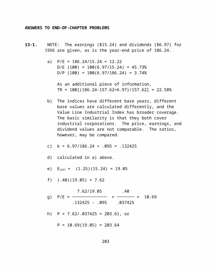
CHAPTER OVERVIEW
Chapter 16 is a straightforward discussion of technical analysis without going too far in trying to explain the myriad details involved in doing technical analysis. As such, it is a good balance between the tools and techniques typically discussed and used in sources that investors might see and the exact steps involved in implementing them. The focus is on a basic description of the techniques and a look behind the concepts involved.
The what and why of technical analysis is developed at the beginning of the chapter, including an overall framework for technical analysis. This discussion provides a foundation for an overall understanding of the subject.
The chapter is organized along two major themes. The first involves stock price and volume techniques. We start with the Dow Theory and then consider charts of price patterns. Again, only the highlights are included because of the voluminous nature of this material and the difficulty in knowing what is the correct interpretation to present. Included here are the best known patterns of stock prices as presented by an article in the popular press. Moving averages are covered here, as is relative strength.
The second organizational theme is technical indicators, such as the advance-decline line, new highs and lows, volume, sentiment indicators as illustrated by the short-interest ratio, the opinions of investment advisory services, mutual fund liquidity, and the CBOE put/call ratio. Each of these indicators is explained in enough detail to make them understandable without getting bogged down in too many how-to details.
An important part of this chapter involves the testing of technical analysis strategies. It is very important to understand how to construct proper tests of various techniques advocated in investments literature. Finally, some conclusions about technical analysis are presented in detail in order to get students thinking about the issues and the logic of technical analysis.
246

Chapter 16 seeks a balance between the conceptual and the descriptive. It attempts to make a fair presentation of the case for technical analysis, but makes it clear that skepticism is warranted although the techniques have not been completely refuted. Ideally, students will come away with an understanding of what must occur for technical analysis to work, and the likelihood of that occurring. Hopefully, they will think logically about what is involved here, and how likely it is to really work--particularly in the case of charts of stock prices.
Clearly, this chapter can be related back to Chapter 12 concerning market efficiency.
CHAPTER OBJECTIVES
To present the basics of technical analysis so students will know what it is all about.
To outline the major techniques and tools of technical analysis so that students can properly classify them.
To present the conceptual issues involved in technical analysis so that students will think about what is being done, and the likelihood of success.
247
MAJOR CHAPTER HEADINGS [Contents]
What is Technical Analysis?
[the use of market data: price and volume information; what technicians believe; a summary of key points about technical analysis]
A Framework for Technical Analysis[diagram outlining the framework; market vs. individual stocks; techniques vs. charting]
Stock Price And Volume Techniques
The Dow Theory[bull and bear market; primary and secondary movements; discussion of how the theory is typically interpreted; criticisms of the theory]
Charts of Price Patterns[support and resistance levels; bar and point-and-figure charts; some evidence on price charts by Levy]
Moving Averages[50-day and 200-day moving averages; signals]
Relative Strength[strength of a stock relative to an index; how relative strength is often used; chart depicting relative strength]
Using the Computer for Technical Analysis[sources of charts, widespread availability]
Technical Indicators
Breadth Indicators[Advance-Decline line is compared to a market average; new highs and lows--how these are used as signals; volume--high trading volume is generally a bullish sign]
245

Sentiment Indicators[short-interest ratio; the opinion of investment advisory services; mutual fund liquidity; CBOE put/call ratio]
Testing Technical Analysis Strategies
[adjustments necessary to conduct a fair test of a trading rule; discussion of filter rules]
Some Conclusions About Technical Analysis
[logical reasons why it probably does not work]
POINTS TO NOTE ABOUT CHAPTER 16
Tables and Figures
There are no tables in Chapter 16. There is no boxed insert.
Figure 16-1 is designed to organize the chapter, outlining the technical analysis approach to common stock selection.
Figure 16-2 illustrates the Dow Theory and can be omitted from discussion if desired.
Figure 16-3 is new to the 8th edition. It illustrates graphically support and resistance levels, and shows a breakthrough. These terms are relatively important in technical analysis, and this graph should facilitate a better understanding of them.
Figure 16-4 illustrates bar charting. Individual instructors will have to decide how much emphasize to give this material. This figure is designed to show students the basics of a chart of stock prices.
Figure 16-5, from a popular press article, illustrates the important price patterns for investors when using charts. This will give students a good feel for what many technicians are typically searching for when they study charts of stock prices.
246
Figure 16-6 illustrates a point-and-figure chart. The same discussion presented above for Figure 16-3 applies here. This type of chart is much less important than the bar chart to most technicians, and can be commented on very quickly, if at all.
Figure 16-7 shows a bar chart for Coca Cola and illustrates moving averages as they are often shown in technical analysis. In this case both a 50-day and a 200-day moving average are shown. This figure is taken from Yahoo and illustrates the type of technical analysis material readily available on the internet.
Figure 16-8 illustrates the relative strength technique. This technique is widely seen (for example, in the chart of each company covered by Value Line). Relative strength can be calculated in various ways.
247
ANSWERS TO END-OF-CHAPTER QUESTIONS
16-1. The rationale of technical analysis can be summarized as:
(a) Prices are determined by the forces of demand and supply.
(b) Many factors affect demand and supply, including fundamental factors as well as market psychology factors.
(c) Stock prices tend to move in trends as they adjust to a new equilibrium level.
(d) Trends can be analyzed, and changes in trends detected, by studying the action of price movements and trading volume over time.
16-2. Fundamental analysis uses a present value model (or, alternatively, a P/E model) to produce an estimate of a stock’s intrinsic value, which is then compared to the market price. It is based on fundamental economic variables such as earnings and dividends.
Technical analysis involves the use of published market data (price and volume information) to predict short-term price movements in either individual stocks or the market. Technicians attempt to forecast trends in price changes.
16-3. Technicians assume that there is a gradual adjustment of stock prices from one equilibrium to another. As this adjustment occurs, prices tend to move in trends.
16-4. Price and volume are the primary tools of the technical analyst. Volume data are used to gauge the general condition in the market and to help assess its trends. Thus, volume information is used in conjunction with price information to help confirm rising or falling trends.
16-5. The Dow Theory is used to predict movements in the stock market. Specifically, it is designed to detect the start
248
of a primary movement (a broad market movement that lasts years).
The confirmation signal is important in interpreting the Dow Theory. A movement is not validated until the Transportation Average confirms the primary movement in the Industrials. The trend will continue as long as the averages confirm each other. (The determination of confirmation, however, is up to each user.)
16-6. The Dow Theory does not forecast how long the primary movement will last.
16-7. With a moving average, a general sell signal occurs when actual prices decline through the moving average on high volume.
16-8. The advance-decline line measures (on a cumulative basis) the net difference in the number of stocks advancing in price and the number of stocks declining in price. The net advance (or decline), therefore, reflects the breadth of the market, or whether the majority of issues are rising or declining in price.
16-9. A contrarian should react in the opposite direction of the sentiment exhibited by investment advisory services. The reason for this is attributed to the fact that these services tend to follow trends rather than forecast them. They are reporting and reacting to what has happened rather than concentrating on anticipating what is likely to happen.
16-10. The rationale for the traditional theory of contrary opinion is that some investors almost always lose. These investors include the small investor, supposedly unsophisticated and usually wrong in his or her actions. The idea is to trade opposite (contrary) these investors.
A newer theory (e.g., Dreman’s) of contrary opinion is that most investors, including institutional investors, are often wrong and that it pays to do the opposite of what they are doing. One way to do this is to buy low P/E stocks, which are not popular at the time.
16-11. The odd-lot index is calculated as:
249
odd-lot sales odd-lot index = ───────────────── odd-lot purchases
A decline in this index indicates more purchases (relative to sales) by small investors. Therefore, according to contrary opinion, it is time to sell and go against this group.
16-12. A rising short interest ratio is considered to be a bullish indicator because a high short interest represents a large number of shares that must be repurchased in order to close out the short sale. The larger the short sale ratio, the larger the potential demand that is indicated.
16-13. A bar chart is the simplest chart in technical analysis. Price is on the vertical axis and time on the horizontal axis. Each day’s price movement is represented by a vertical bar whose top (bottom) shows the high (low) price for the day. The bottom of a bar chart usually shows the trading volume for each day. Time intervals can be days, weeks, months, or anything else.
A point-and-figure chart shows only significant price changes, with volume omitted completely. Although the horizontal axis is time, specific calendar time is unimportant. X’s are typically used to show upward movements, and O’s to show downward movements. The X or O is recorded only when the price moves by a specified amount.
16-14. Relative strength is generally used to forecast individual stocks or industries. It is calculated as the ratio of a stock’s price to a market index, an industry index, or the average price of the stock itself over some previous period. These ratios are plotted to form a graph of relative price across time. A rising ratio indicates relative strength, and it is often assumed that the trend will continue.
16-15. Assume a chart pattern is predictive in the sense that each time it gives a signal it correctly predicts
250
movements in price. More and more investors will start to use it as they observe what is happening. This is a destructive process because price will reach its equilibrium value quickly, taking away profit opportunities from all but those acting the fastest. Also, some participants will try to anticipate the pattern or signal, driving price to an equilibrium even more quickly. Eventually, the value of this predictor will be negated.
16-16. No! It is not possible to test all the techniques of technical analysis and their variations and interpretations because they are too numerous! Therefore, absolutely definitive statements cannot be made.
16-17. In order to scientifically test a claim of success using technical analysis, an alternative needs to be constructed. For example, can this technician outperform a buy-and-hold strategy consisting of stocks from the same population used by the technician, on a risk-adjusted basis, over some period of time (preferably years) after all relevant costs are accounted for?
16-18. The traditional contrarians focused on the small investors such as the old-lotters. The new contrarians tend to go against the “crowds” in general, including “sophisticated” investors such as institutional investors.
16-19. No inherent reason exists for stock price movements to repeat themselves. However, by sheer chance alone, some probability exists of a pattern repeating itself.
16-20. It does present enough data to show some secondary reactions, and a penetration of a previous high or low. However, it would be highly desirable to use more data.
16-21. This chart contains both the industrial and transportation averages (as well as the utilities average and volume figures). The latter is needed to confirm any signal given by the industrial average.
16-22. Increased trading in stock options and financial futures has caused the short interest ratio to be less reliable.
251
These instruments provide investors with new ways to hedge and speculate, and they have helped to distort the historical boundaries for the short interest ratio.
16-23. A buy (bullish) signal is generated when actual prices rise through the moving average on high volume.
A sell (bearish) signal is generated when actual prices decline through the moving average on high volume.
A rising advance-decline line, in conjunction with a decline in a market average, suggests that the decline in the latter should reverse itself. If the market average rises while the advance-decline line weakens or declines, a fall in the market is expected.
16-24. This figure was produced using a random number generator; therefore, in answering (a) and (b), any patterns are purely coincidental. As for (c), any guess is as good as another. Finally, in (d), the answer is obviously yes since this chart was produced by such a process.
CFA16-25. b
CFA16-26. a
CFA16-27. d
CFA16-28. c
CFA16-29. a
252
PART VI: DERIVATIVE SECURITIES
Chapter 17: Options
CHAPTER OVERVIEW
253
Chapter 17 is a complete and detailed analysis of options--puts and calls--including market index options. It is designed to cover all the terminology and trading mechanics as well as considerable analytics involving the valuation and use of options. It can be used with software for solving the Black-Scholes call option model, although use of the software is optional because complete examples are presented to illustrate the model. Such concepts as put-call parity and hedge ratios also are covered. Overall, this chapter is a comprehensive treatment of options from the standpoint of the typical undergraduate student. It is also a very lengthy chapter.
The first few pages of the chapter provide the necessary background information, including terminology and an analysis of exactly how options work, with an extended example. The mechanics of trading also are covered, including a detailed description of the role of the clearing corporation, margin, and brokerage commissions.
The payoffs and profits from basic option positions are analyzed in detail, using graphs, in order for students to clearly understand how options can be used and how they change the distribution of potential outcomes in ways that could not readily be accomplished (if at all) without the use of options. Each of the four basic cases is analyzed, buying a call and buying a put, and selling (writing) a call and selling a put. Somewhat more sophisticated options strategies are examined in a briefer format in Appendix 17-A by considering straddles, strips, straps, and spreads. While the basics are covered here, the instructor may choose to augment this discussion. At the beginning level, however, it is sufficient as presented.
Considerable attention is devoted to option pricing. The discussion begins with a general framework of in-the-money and out-of-the money conditions, and the resulting intrinsic value of an option. The speculative premium is then developed. Examples are used in all cases, and these examples are based on option prices as might be seen in The Wall Street Journal.
The next part of the discussion on option pricing develops the boundaries on option prices in graph format, which provides a framework for understanding actual option prices. This discussion leads into the Black-Scholes model, which is developed in a detailed but understandable format. All of the variables
254
are explained, and a comprehensive example illustrates the calculations. Following this, the idea of hedge ratios is developed, and the put-call parity relationship presented.
Having developed all of the above, the chapter proceeds to explain what puts and calls mean to investors in terms of truncating the distribution of potential returns and the concept of purchasing insurance. This is followed by a discussion of portfolio insurance, with a detailed example that clearly illustrates this often-talked about concept. Finally, the evolutionary use of options is discussed, as we consider how institutions are using options.
Chapter 17 concludes with a thorough discussion of stock index options. Basics are covered, and examples given. Strategies with stock index options are developed, showing how investors might use these instruments in managing their portfolios.
Appendix 17-A covers spreads and options. This material is placed in an appendix because Chapter 17 is a long chapter, and this material is not absolutely necessary for students to obtain a basic knowledge of options.
Appendix 17-B contains a quite-detailed discussion of warrants for those who wish to cover this subject.
CHAPTER OBJECTIVES
To present the necessary background--terminology and mechanics--to thoroughly understand puts and calls.
To explain uses of, and strategies with, options.
To explain the pricing of options.
To present a complete basic discussion of stock index options.
255
MAJOR CHAPTER HEADINGS [Contents]
Introduction
[definitions; why options markets?]
Understanding Options
Options Terminology[strike price, expiration date, option premium; LEAPS; reading The Wall Street Journal]
How Options Work[detailed examples of buying and selling calls and puts]
The Mechanics of Trading[secondary markets; the clearing corporation]
Payoffs And Profits From Basic Option Positions
Calls[buying a call; selling a call; diagrams]
Puts[buying a put; writing a put; diagrams]
Some Basic Options Strategies
Covered Calls[explanation and example; diagram]
Protective Puts[explanation and example; diagram]
Portfolio Insurance[explanation; discussion; example; costs]
256
Option Valuation
A General Framework[in the money and out of the money definitions]
Intrinsic Values and Time Values[intrinsic value definition and examples]
Boundaries on Option Prices[graphical illustration of how boundaries are established]
The Black-Scholes Model[model variables and equations; analysis of the inputs; complete example]
Put Option Valuation[using put/call parity to derive the price of a put]
Summarizing the Factors Affecting Options Prices[effects of various variables on put and call prices]
Hedge Ratios[definition; example]
Using the Black-Scholes Model[brief analysis of the evidence]
An Investor’s Perspective on Puts and Calls
What Puts and Calls Mean to Investors[truncating the distribution of returns]
The Evolutionary Use of Options[institutional trends; use in strategic portfolio management]
Stock Index Options and Interest Rate Options
[mention of interest rate options]
The Basics of Stock Index Options[what is available; differences from stock options; example]
257

Strategies with Stock Index Options[example of buying a call; example of buying a put]
The Popularity of Stock Index Options
Appendix 17-A Spreads and Combinations
Appendix 17-B Warrants
POINTS TO NOTE ABOUT CHAPTER 17
Tables and Figures
Table 17-1 analyzes how the relevant variables affect both put and call prices.
Figures 17-1 through 17-5 illustrate the basic options strategies (buying and writing puts and calls) and can be used to emphasize important points about the distribution of returns. Both the payoff profiles and the profit and losses are shown for each case.
Figure 17-6 shows the payoff profiles for a covered call position, while Figure 17-7 shows the profit and loss possibilities for a covered call position.
Figure 17-8 illustrates the payoff profile and profit/loss possibilities for a protected put position.
Figure 17-9 illustrates the boundaries on option prices.
Box Inserts
Box 17-1 is a good popular press discussion of how to use puts to protect positions during a bear market. It has a good general discussion of options, an effective analysis of puts, and very clear examples.
258
ANSWERS TO END-OF-CHAPTER QUESTIONS
17-1. Puts and calls are short-term options, with maturities (on organized exchanges) measured in months. Warrants generally have maturities of several years, and a few are perpetual.
A second distinction is that puts and calls are created by investors (individuals or institutions), while warrants are created by corporations.
Finally, every warrant is unique, with the corporation (issuer) setting its parameters on a case-by-case basis.
17-2. The potential advantages of puts and calls include:
(a) the smaller investment required relative to transacting in the common
(b) leverage--potential magnification of gains
(c) maximum loss is known in advance
(d) an expanded opportunity set, increasing the risk-return combinations available.
(e) possible lower transactions cost for the portfolio as a whole
(f) the ability to hedge or speculate on broad market movements and/or interest rates using index options
17-3. (a) Strike or exercise price--the per-share price at which the common stock may be purchased (or sold to a writer)
(b) Naked option--a call option written without the stock being owned by the writer, or a put option written by a writer who is not short the stock
(c) Premium--the price paid by the option buyer to the writer or seller of the option--the market price of the option
259
(d) Out-of-the-Money Option--a call whose exercise price exceeds the current stock price or a put
whose exercise price is less than the current stock price.
17-4. Investors, both individuals and institutions, write puts and calls in an attempt to profit from their beliefs about the underlying stock’s likely price performance. Writers earn the premiums paid by the buyers.
17-5. The options clearing corporation (OCC) plays an important role in the options market. The OCC guarantees the performance of the contracts, preventing potential problems with writers who must honor their obligations. The OCC facilitates the taking of an opposite (closing) position at any time by buyers or sellers.
17-6. Option prices almost always exceed intrinsic values. This excess, sometimes called the premium over parity, exists because buyers are willing to pay some price for potential future stock price movements.
17-7. Option prices almost always exceed intrinsic values, with the difference reflecting the option’s potential appreciation typically referred to as the time value. Time obviously has a positive value for call options because the longer the time to expiration for a call option, the more chance it has to appreciate.
17-8. The Black-Scholes model uses five variables to value a call option:
(a) the price of the underlying stock(b) the exercise price of the option(c) the time remaining to the expiration of the option(d) the riskless rate of return(e) the volatility of the underlying stock price.
The first two variables determine whether an option is in-the-money or not. A difference between (a) and (b) that results in an in-the-money option has a direct (positive) effect on the option’s value.
260
The last three factors, (c) through (e), have a direct (positive) effect on an option’s value.
17-9. Reasons for purchasing a call are:
(a) to establish a position with minimum initial investment
(b) to protect a short sale
(c) to maximize leverage for speculative purposes
(d) to engage in hedging strategies.
17-10. Investors writing calls often are seeking the income from the premium. Such a strategy can supplement the dividend income on stocks held.
The obligation of a call writer is to deliver the stock for the strike price if called upon to do so.
17-11. A straddle (see Appendix 17-A) is a combination of a put and a call on the same stock with the same exercise date and exercise price.
A straddle buyer believes that the underlying stock price is highly volatile, and may go either up or down. Since each part of the straddle can be exercised separately, a buyer can profit from a large enough move either way.
17-12. A spread (see Appendix 17-A) is defined as the purchase and sale of an equivalent option varying in only one respect (exercise price or expiration date). The purpose of a spread is to reduce risk in an option position.
17-13. Two types of spreads are (see Appendix 17-A):
(a) A money spread involves the purchase of a call option at one exercise price and the sale of the same maturity option, but a different exercise price.
(b) A time spread involves the purchase and sale of options identical except for expiration dates.
261

17-14. The call or put writer’s position is considerably different from the buyer’s position because of the obligation involved on the part of a writer. A call writer must be prepared to deliver the stock, regardless of the level to which the stock price has risen. A put writer must be prepared to take delivery of a stock and pay a specified price for it, regardless of the level to which the stock price has declined. Buyers know their potential losses while writers do not.
17-15. A stock index option is a call or put contract on a stock market index. Stock index options enable investors to trade on general stock market movements in the same way that they can trade on individual stocks.
Stock index options have included the S&P 100 Index, the S&P 500 Index, the New York Stock Exchange Index, the Major Market Index, the Value Line Index, the National OTC Index, and various industry sub-indices such as the Computer Technology Index and the Gold/Silver Index. Index options were also available for an Institutional Index and a NYSE Beta Index. This list changes from time to time; therefore, it is best to consult the current issue of The Wall Street Journal.
17-16. The major differences between a stock index option and a stock option is that buyers of index options receive cash from the seller upon exercise of the contract. Stock options, in contrast, require the actual delivery of the stock upon exercise.
17-17. A put can be used to protect a profit that an investor has. Assume a stock purchased at $100 rises to $130. To protect against a decline, an investor may be able to purchase a put with an exercise price of $130 which would offset the lost profits should the stock price decline.
A call could be used to protect a short sale position. To protect against an unexpected rise in price, an investor could purchase a call. If the stock price rises, the call can be exercised and the stock acquired and delivered to cover the short sale.
17-18. Writing covered calls is basically a conservative strategy. The writer forgoes possible price appreciation
262
while knowing what the likely gains are, whether the stock is called or not.
For a naked call writer, the potential gain is limited while the potential loss is large.
17-19. Return volatility is greater because the options sell at relatively small prices. Thus, the returns on options as a percentage of the invested funds is larger than for the corresponding common stock.
17-20. With industry sub-index stock index options, investors can speculate on certain segments of the market. Thus, if an investor is optimistic about the technology stocks, a call on the Computer Technology Index can be purchased; if pessimistic about the prospects of such a group, a put can be purchased. And so forth.
17-21. (a) If you fear a market decline over a six month period, you could purchase a put on one of the market indices, thereby establishing a short position.
(b) Basically, this hedge would be quite effective. However, the exact degree of effectiveness will depend upon how closely correlated the 50 stock portfolio is with the particular market index involved. For example, if most of the stocks in the portfolio were on Nasdaq, a put option on the NYSE Composite Index would not be as effective as if the 50 stocks were large NYSE stocks.
(c) Other things being equal, as the number of stocks in the portfolio increases, the protection should be more effective because the portfolio resembles more and more the market as a whole.
17-22. If you expect interest rates to rise, you could purchase an interest rate option put. If interest rates are expected to rise, bond (i.e., fixed income securities) prices will decline; therefore, you need a put.
17-23. To say an option is worth more alive than dead refers to the fact that it never pays to exercise an American call option on a non-dividend-paying stock early.
263
Consider such an option holder who is ready to close out the position. The holder has two choices: exercise the call or sell it. It can be shown that the proceeds from the sale of the option exceed the proceeds from exercising. Thus, the option should be continued by selling it rather than “killing” it through exercise.
CFA17-24. a
CFA17-25. a
CFA17-26. a
CFA17-27. a
CFA17-28. a
CFA17-29. a
CFA17-30. b
264
ANSWERS TO END-OF-CHAPTER PROBLEMS
17-1. (a) The Teledyne calls that are in the money, given a closing stock price of $162, are the calls with exercise prices of 140, 150, and 160.
(b) The Teledyne puts in the money are the puts with exercise prices of 170 and 180.
(c) Although the stock closed at $162, investors are willing to pay 1/4 for the 180 call because they feel there is some probability that the price of the stock will rise to the 180 area. They are willing to pay only 1 for the 150 put because they feel there is less chance of the stock declining to the 150 area.
17-2. (a) Using the Teledyne data, the intrinsic value of the April 140 call is
162 - 140 = 22
The intrinsic value of the October 170 call is $0 (zero) since the stock price is less than the exercise price.
(b) The intrinsic value of the April 140 put is $0 (zero) since the strike price is less than the stock price.
The intrinsic value of the October 170 put is
170 - 162 = 8
(c) The stock price is on the higher end of the range of exercise prices available for Teledyne options. Therefore, the intrinsic values for the calls are greater.
17-3. (a) The cost of 10 October 150 call contracts in total dollars is: a price of 25 = $2500 per contract; therefore, 10 contracts would involve a total dollar amount of $25,000. From the text, the brokerage cost for 10 option contracts is $65.
284

Therefore, the total cost of this transaction would be $25,065.
(b) The cost of 20 October 160 put contracts in total dollars is: a price of 9 = $900 per contract; therefore, 20 contracts would involve a total dollar amount of $18,000. From the text, the brokerage cost for 20 contracts is $115. Therefore, the total cost of this transaction would be $18,115.
(c) If Teledyne closed at $164 the following day, the in-the-money call options would increase in value, and the out-of-the-money calls probably would also. As the stock price rises, the prices of the put contracts should decline.
(d) If the price of this option rises $1, from 25 to 26, the gross profit per contract would be $100. Therefore, for 10 contracts the one-day profit would be $1000. Subtracting out two-way brokerage cost of 65 x 2 = $130, an investor would net $870.
(e) If the October 160 put goes to 7 1/2, each contract would show a loss of 9 - 7 1/2, or 1 1/2 ($150). Therefore, the one-day loss on 20 contracts would be $150 x 20 = $3000. Adding in two-way brokerage costs of $115 x 2 = $230, the total loss would be $3230 if these contracts had been bought at 9 and sold one day later at 7 1/2.
(f) These contracts, like any option contracts, can expire worthless, resulting in a total loss of investment plus brokerage costs. You can lose the full purchase price plus at least one-way commissions.
17-4. (a) More, because of its longer time to maturity.
(b) $3--the intrinsic value is zero.
(c) Using the put-call parity relationship, the price of a put is:
285
price of put = EP/(ert) - CMP + CP
= $50/(e.08(.25)) - $45 + $3
= $50/1.0202013 - $45 + $3
= $7.01
NOTE: e.08(.25) = .02 raised to the ex.
It is not working according to this calculation.
17-5. Using the put-call parity relationship, the price of a put is:
price of put = EP/(ert) - CMP + CP
= $45/(e.08(.25)) - $47.375 + $8.94
= $45/1.0202013 - $47.375 + $8.94
= $5.67
NOTE: e.08(.25) = .02 raised to the ex.
NOTE: THE REMAINING PROBLEMS WERE SOLVED WITH software. Numerous alternative software packages for solving options problems are available.
17-6. Price of call = $7.30Price of put = $1.53
17-7. (a) $7.84(b) $10.65
The change in volatility caused the greater change in the value of the call. In general, call prices are going to be more sensitive to a change in volatility than in a change in the risk-free rate.
17-8. The hedge ratio as determined by the program is -0.66. Therefore, for every call option written, 0.66 shares of common would be required to hedge the position. For a standard 100-share option contract, 66 shares of common would be required.
286
17-9. (a) $20.66(b) $14.44(c) $6.63
17-10. If the stock is currently $2 out of the money, it is selling for $38. Using this price and the information given, the price of the call is calculated to be $6.31.
17-11. The put would sell at a higher price because it would be in the money since the stock price is less than the exercise price. Solving for the price produces a value of $7.33.
Chapter 18: Futures
287
CHAPTER OVERVIEW
Chapter 18 is designed to cover the basics of futures markets in general but with primary emphasis on financial futures. While the basics are applicable to any commodity, and money can be thought of as another commodity, it is felt that students will receive the most benefit from concentrating on financial futures after a general introduction to the subject, which is one of the more difficult subjects for beginners.
The first part of the chapter develops the idea of a forward market and a futures market, outlines current U. S. futures markets, and describes the structure of futures markets. This provides the student with the necessary background information.
The chapter next focuses on the mechanics of trading, including all of the basics. Margin, which is completely different from that involving stocks, is developed in detail, including an example.
The chapter discusses the use of futures contracts by explaining the role of hedgers and speculators. This includes a description of basis. The subsequent discussion is organized by examining how to both hedge and speculate in both interest rate futures and stock index futures. The necessary background information is provided, along with examples of how to use the contracts, with particular emphasis on short hedges. The limitations of hedging are considered. Speculating with both interest-rate futures and stock-index futures is discussed.
The chapter concludes with a discussion of program trading, which is often cited in the popular press.
288
CHAPTER OBJECTIVES
To explain the basics of futures markets in general.
To explain financial futures in particular--what is available, how they are used, what they can accomplish.
To illustrate various hedging and speculating strategies using both interest rate options and stock index options.
MAJOR CHAPTER HEADINGS [Contents]
Understanding Futures Markets
Why Futures Markets?[reasons for forward markets and futures markets]
Current U. S. Futures Markets[futures markets as classified in The Wall Street Journal]
Foreign Futures Markets[brief description of futures markets in other countries]
Futures Contracts[basic characteristics]
The Structure Of Futures Markets
Futures Exchanges[members of the exchanges]
The Clearinghouse[the role of the clearinghouse]
289
The Mechanics of Trading
Basic Procedures[short position vs. long position; offset; price fluctuations; commissions]
Margin[good faith deposit; margin call; how accounts are marked to the market, including example]
Using Futures Contracts
[traditional uses]
Hedgers[trying to offset the risk in a cash position]
How to Hedge With Futures[basic idea; short hedge; long hedge]
Speculators [trying to profit by their actions]
Financial Futures
[reasons for; differences between these and commodity futures]
Interest Rate Futures[what contracts are available; reading quotes; hedging and speculating with interest rate futures, with examples]
Stock-Index Futures[how they work; hedging with stock-index futures; how short hedges work; example; long hedges; limitations of hedging with stock index futures; index arbitrage and program trading; speculating with stock index futures--benefits; strategies--spreaders (intramarket and intermarket]
290
Appendix 18-A Futures Options
POINTS TO NOTE ABOUT CHAPTER 18
Tables and Figures
Exhibit 18-1, showing the types of futures contracts available, is for general reader interest.
Table 18-1, showing how investor accounts involving futures are marked to the market, is worth emphasizing because it helps to explain the real risk of futures contracts--the equity can be wiped out, or diminished severely, very quickly.
Exhibit 18-2 on characteristics of interest rate futures contracts can be examined by students on their own.
Exhibit 18-3 on hypothetical quotes on bond futures contracts also provides basic information.
Exhibit 18-4 illustrates a short hedge for interest rate futures. The major emphasis should be on the short hedge since most investors are long the cash position and must hedge by selling futures.
Table 18-2 illustrates both short and long hedges using stock-index futures. Although designed to be simple examples, they convey the essence of the hedge involved, and students can readily understand them.
Figure 18-1 shows return distributions for hedged and unhedged positions on a conceptual basis. The idea, of course, is to show why investors might choose to hedge their positions.
Figures 18-2 through 18-4 are worthwhile as transparencies to reinforce the points illustrated and provide the basis for classroom discussion.
• Figure 18-2 shows that the value of a well-diversified stock portfolio tracks very closely the price of the S&P 500 index futures.
291
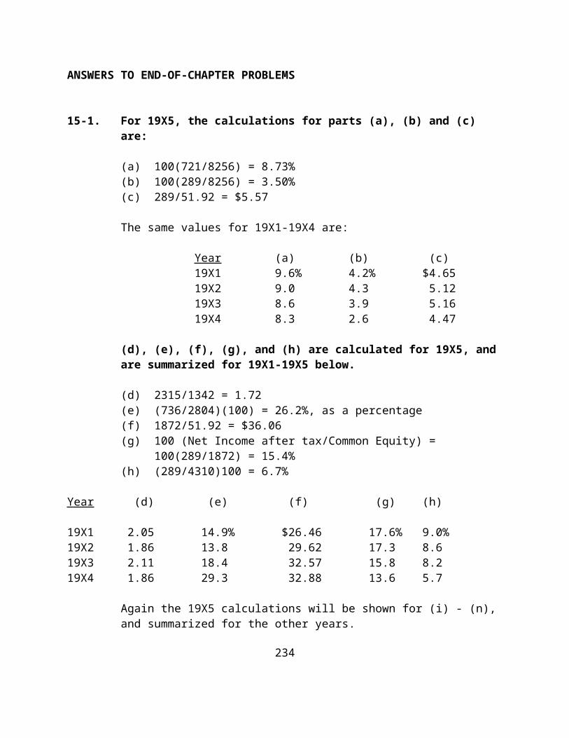
• Figure 18-3 shows the value of a well-diversified portfolio versus the value of the same portfolio hedged by sales of S&P 500 index futures--the hedged portfolio is much less volatile than the unhedged portfolio.
• Figure 18-4 (a) compares the value of a relatively undiversified portfolio with the price of the S&P 500 futures contract. This portfolio is only 66 percent diversified, and the futures contract does not move all that closely with the portfolio.
Figure 18-4 (b) shows that a hedged position in this situation is only 27 percent lower than an unhedged position. Thus, stock-index futures generally do not provide a good hedge for relatively undiversified portfolios.
NOTES ABOUT APPENDIX 18-A
This appendix, which covers futures options, can easily be omitted without any loss of continuity. It is provided for the sake of completeness for those who want to cover this topic. Because of time constraints and because of the difficulty of the subject, many instructors choose to skip this topic. Perhaps the best approach is to simply acknowledge the existence of these instruments but not spend time discussing them.
292
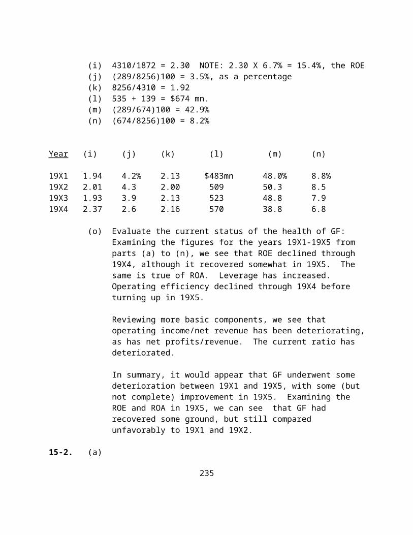
ANSWERS TO END-OF-CHAPTER QUESTIONS
18-1. A futures contract is a commitment to buy or sell at a specified future settlement date a designated amount of some item. A firm agreement by two parties, the seller of the futures contract agrees to make delivery, and the buyer agrees to take delivery, at a currently determined market price.
18-2. All futures contracts are marked to the market daily; that is, all profits and losses on a contract are credited and debited to each investor's account every trading day.
Almost all (95%+) futures contracts are settled by offset rather than delivery; that is, holders liquidate a position by arranging an offsetting transaction.
18-3. The clearinghouse ensures the fulfillment of each futures contract. Buyers and sellers settle with the clearinghouse, not with each other. The clearinghouse is on the other side of all transactions, and stands ready to fulfill a contract if either buyer or seller defaults. Thus, the clearinghouse helps to facilitate an orderly market in futures.
18-4. The initial margin deposited with a broker is the equity of the transactor. Each contract also requires a maintenance margin below which the investor’s equity cannot drop. If the equity declines below the maintenance margin, a margin call occurs. It should be remembered that all contracts are marked to the market daily; that is, all profits and losses are debited and credited daily to an investor’s account.
18-5. Differences between trading in stocks and trading in futures contracts include:
(a) The whole concept of margin is different because no credit is being extended with futures contracts.
(b) Margin is the norm in futures but not in stock trading.
293
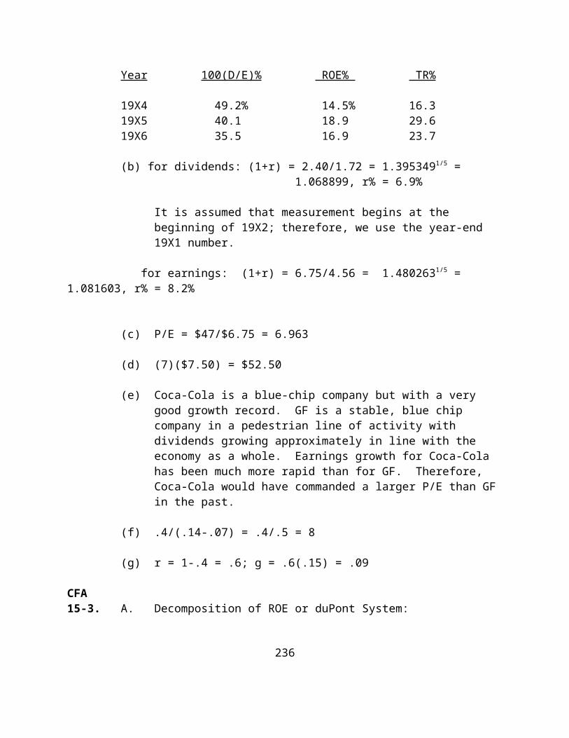
(c) Most futures contracts have a daily price limit while stocks do not.
(d) Unlike stocks, there are no price movement restrictions with short sales.
(e) Futures positions have definite termination dates.
(f) Brokerage commissions for futures are paid on the basis of a completed contract, unlike stocks.
(g) There are no specialists on futures exchanges.
(h) Futures contracts are not securities.
18-6. Financial futures differ from other futures contracts in a few respects.
With stock index futures, the seller settles in cash at maturity--there is no delivery. Also, unlike traditional futures contracts, stock index futures typically have no daily price limits.
18-7. Hedgers buy or sell futures contracts in order to offset the risk in some other position. They want to reduce the risk of adverse price fluctuations. Hedgers forego some potential profits to eliminate part of the risk.
Speculators buy or sell futures contracts in an attempt to earn a return. They are willing to assume the risk of price fluctuations, hoping to profit from them.
18-8. Basis can be, and is, defined in different ways. In this edition basis is defined as the difference between the cash price of an item and the futures price of the contract used, and the basis is positive when this difference is positive.
18-9. Price quotations on Treasury bonds are percentages of par, are quoted in 32nds, and the face value is $100,000. Therefore, a price of:
80-5 is 80 5/32 of $100,000 or $80,156.25
294
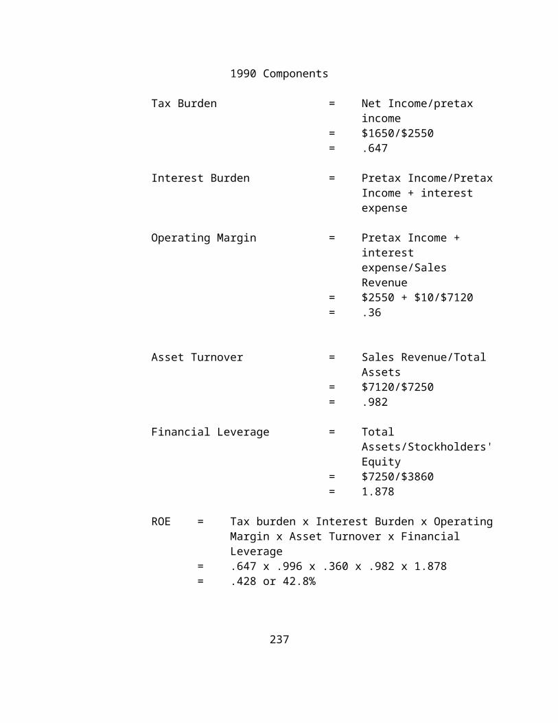
90-24 is 90 24/32 of $100,000 or $90,750.00
69-2 is 69 2/32 of $100,000 or $69,062.50.
18-10. A manager with a bond position may plan to sell the bonds later but meanwhile fears a rise in interest rates. To protect the portfolio, a short hedge can be used. If interest rates rise (and, therefore, bond prices drop), the manager will gain on the short hedge while losing on the cash position (i.e., the portfolio).
18-11. Risk cannot be entirely eliminated in a hedge because of basis risk. The basis fluctuates in an unpredictable manner, and changes in the basis will affect the hedge position during its life.
18-12. A weighted short hedge adjusts for the differences between the 8% coupon assumed in the Treasury bond futures contract and the coupon bonds actually being held in the portfolio. Higher coupon bonds will cause a greater decline in dollar value relative to the futures contract. A conversion factor is available to adjust hedge amounts.
A straight short hedge, on the other hand, would simply match the dollar value of the portfolio with the number of $100,000 contracts that would be comparable.
18-13. Investors could have preferences among the different stock index futures as a result of the composition of their particular portfolios. The New York Stock Exchange Index, covering only NYSE stocks, is not the same as the Value Line Index, which covers NYSE, AMEX, and OTC stocks.
295

18-14. Stock index futures allow investors to hedge systematic (market) risk. This is desirable for investors attempting to earn the unique part of a stock's return while avoiding market risk. The futures contract helps to protect the portfolio against market fluctuations.
18-15. A pension fund could use a long hedge with stock index futures if a market rally was expected but the fund was not ready with individual stock selections. Buying futures contracts would provide gains if the market does rise, and would help to offset the cost of buying stocks at the higher prices existing after the rise.
18-16. • An investor would likely buy a call on a stock index if he or she expected a rise in the market and wanted to try to take advantage of this expectation.
• An investor would likely buy puts on interest rate futures if he or she expected interest rates to rise (which would cause a decline in bond prices).
18-17. Program trading involves the use of computer-generated orders to buy and sell securities based on arbitrage opportunities. The arbitrage occurs between common stocks, on the one hand, and index futures and options, on the other.
Large institutional investors seek to exploit differences between the two sides. Specifically, when stock index futures prices rise substantially above the current value of the stock index itself (e.g., the S&P 500), they sell the futures and buy the underlying stocks, typically in “baskets” of several million dollars.
Because the futures price and the stock index value must be equal when the futures contract expires, these investors are seeking to “capture the premium” between the two, thereby earning an arbitrage profit. That is, they seek high risk-free returns by arbitraging the difference between the cash value of the underlying securities and the prices of the futures contracts on these securities. In effect, they have a hedged position and should profit regardless.
CFA
296
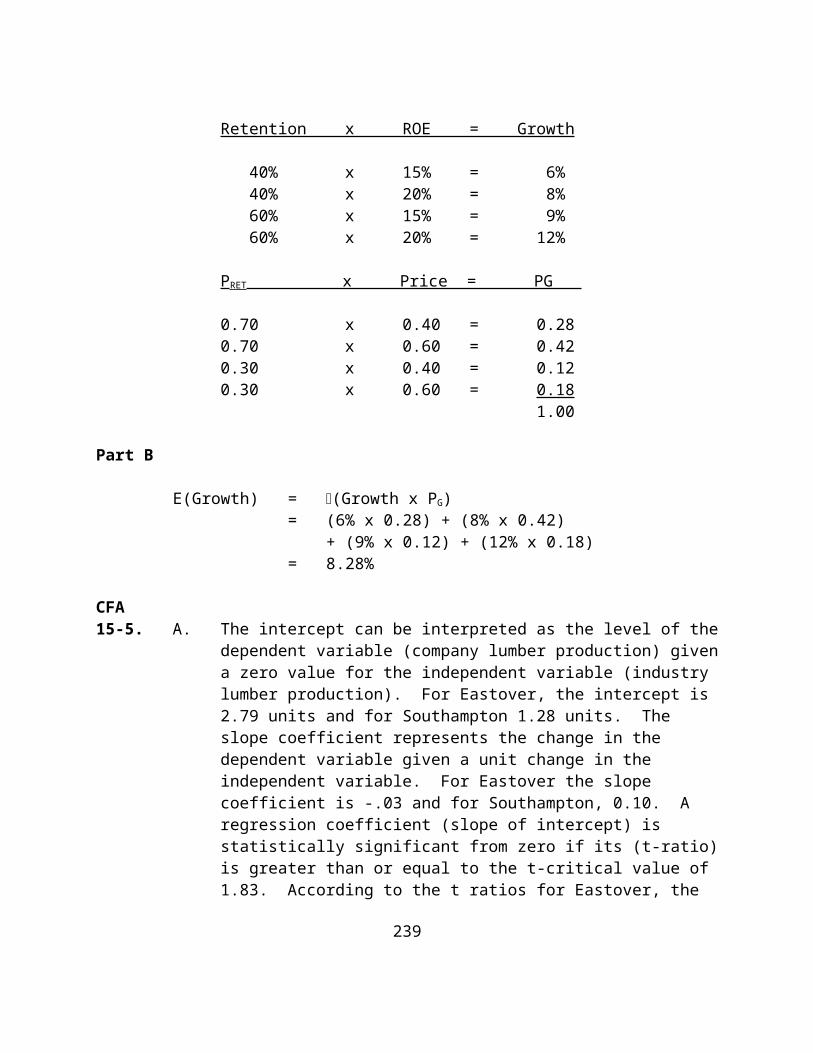
18-18. Call options give the owner the right, but not the obligation, to purchase SFr’s for a pre-specified amount of domestic currency. Purchasing an at-the-money call option would guarantee the current exchange rate over the life of the option. If the SFr declines in value, the call will not be exercised since francs can be purchased more cheaply in the open market and redeeming the bond issue will be less costly.
Contrasting characteristics:
• Currency options are traded world-wide and enjoy a liquid market.
• Exchange-traded currency option contracts have standard amounts, maturities, etc.
• Over-the-counter options could be tailored to meet Michelle's needs.
• The initial cash outflow would be the premium. • The use of options preserves the ability to
profit. • No counterparty credit risk. • Must roll to match 5-year obligation.
Currency forward contracts commit the seller to deliver the specified amount of currency to the buyer on a specified future date at a fixed price. A short position in a forward contract requires delivery.
Contrasting characteristics:
• The market for forward contracts is over-the-counter and sometimes may not be as liquid as option or futures market.
• Forward contracts may be custom-designed for specific applications.
• Cash does not change hands until a forward contract is settled.
• Counterparty credit risk. • Can best match 5-year obligation.
Currency futures are like forward contracts except the gain or loss is settled daily under the supervision of an organized exchange. A short position in the futures requires either offset or delivery at expiration.
297
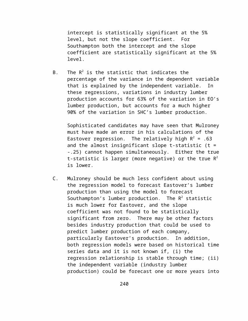
Contrasting characteristics:
• Futures are traded in standardized contracts and are highly liquid.
• Cash is required for daily settlement. • A margin account is required. • Management and administration costs are higher than
with a forward or option contract. • No counterparty credit risk. • Must roll to match 5-year obligation.
CFA18-19. d
CFA18-20. d
CFA18-21. b
CFA18-22. c
CFA 18-23. b
CFA18-24. b
298

ANSWERS TO END-OF-CHAPTER PROBLEMS
18-1. (a) The initial margin is $3500. Each point in price is equivalent to 20 ticks worth $25 each, or $500.
Equity on day of purchase = $3500--the initial position
Equity 1 day after purchase = $3650 [67.8 - 67.5 = .3 or 6 ticks worth $150]
Equity 2 days after purchase = $3800 [68.1 - 67.8 = .3 or 6 ticks worth $150]
Equity 3 days after purchase = $3750 [68 - 68.1 = -.1 or 2 ticks worth -$50]
Equity 4 days after purchase = $4000 [68.5 - 68 = .5 or 10 ticks worth $250]
(b) The excess equity for these four days is +150, +300, +250, and +500.
(c) The final gain is one point, or $500.
(d) An investor who was short over this same period would show the same numbers in reverse; that is, equity shortages and a final loss of $500.
18-2. The aggregate change in market value is the difference between the current price (or closing price) and the initial price multiplied by $500. Therefore
[70.5 - 67.5] X $500 = $1500
18-3. (a) Sell 10 contracts at 82-20 each82-20 = $82,625 and 10 contracts = $826,250
Buy 10 contracts at 76-12 each 76-12 = $76,375 and 10 contracts = $763,750
This is a short position and the price declined. The total profit is $826,750 - $763,750 = $63,000.
299
(b) Sell 10 contracts at 80-14 each80-14 = $80,437.50 and 10 contracts = $804,375
Buy 10 contracts at 77 each77 = $77,000 and 10 contracts = $770,000
This is a short position, and the price declined. The total profit is $804,375 - $770,000 = $34,375.
(c) Buy 15 contracts at 62-1062-10 = $62,312.50 and 15 contracts = $934,687.50Sell 15 contracts at 64-2464-24 = $64,750 and 15 contracts = $971,250
This is a long position, and the price rose. The total profit is $975,250 - $934,687.50 = $40,562.50.
(d) Sell one contract at 70-1470-14 = $70,437.50Buy one contract at 78-0878-08 = $78,250
This is a short position; however, the price rose. The total loss is $78,250 - $70,437.50 = $7812.50.
18-4. (a) The manager is long in the cash market, so to protect this position the manager would establish a short position. At $100,000 per contract, the manager should sell 10 futures contracts with a maturity three months hence (we are ignoring weighted hedges).
(b) The manager sells 10 contracts at a current price of 68, for a total transaction value of $680,000. The manager repurchases 10 of these contracts three months later at a price of 59-12, for a total transaction value of $593,750 ($59,375 x 10). Therefore, this was a successful hedge with a total dollar gain of $86,250.
The futures position gains $86,250.
(c) If the bonds are priced at 67-8 three months later, the cash market position is:
300
beginning -- $76,062.50 X 10 = $760,625 ending -- $67,250 X 10 = 672,500 loss $ 88,125
The portfolio (cash) position declines $88,125.
(d) The net effect of this hedge is a loss of $88,125 - $86,250 = $1875
CFA18-5. Information about foreign firms is often difficult to
obtain on a timely basis and, once obtained, can be difficult to interpret and analyze due to language and presentation differences.
Financial statements are not comparable from country to country. Different countries use different accounting principles. Even when similar accounting methods are used, cultural, institutional, political and tax differences can make cross-country comparisons hazardous and misleading.
Stock valuation techniques useful in the U.S. may be less useful in other countries. Stock markets in different countries value different attributes.
Smith must consider currency risk in selecting non-U.S. stocks for his portfolio.
Increased costs: custody, management fees, and transactions expenses are usually higher outside the U.S.
The candidate must realize that a futures contract is a commitment to transact in the future. The price of the contract on any given day is a function of the current price of the underlying commodity (index price) plus the time value of money less, in this case, any dividends received.
F0 = S0(1 + rj - d)m
Where: F0 = Futures Contract PriceS0 = Index Price = 15,000rj = Risk Free Rate = .05d = Dividend Yield = .02
301
m = Length of Contract (years) = .5
Therefore:
F0 = 15,000(1 + .05 - .02)0.5
F0 = 15,223
ANSWERS TO APPENDIX 18-A
18A-1. (a) greater than(b) greater than(c) less than(e) less than
Chapter 19: Portfolio Selection
CHAPTER OVERVIEW
302
Chapter 19 is a follow-up to Chapter 7, which discussed the basics of Markowitz portfolio theory in terms of the expected return and risk of a portfolio. Chapter 19 concludes this discussion by analyzing the efficient frontier, the Single Index Model simplification of the efficient frontier, how the efficient frontier is changed by borrowing and lending, and the Separation Theorem. This organizational structure allows students to concentrate on related ideas together, and does not overwhelm them all at once with the complete details of this important material.
Chapter 19 begins by discussing the steps involved in building a portfolio of financial assets. The chapter follows these steps.
The first step is to use the Markowitz portfolio selection model to choose an efficient portfolio. The efficient set of portfolios is explained in detail, including the necessary information about indifference curves. This discussion concludes with matching indifference curves (preferences) with the efficient set (possibilities). Important points about the Markowitz analysis that often cause confusion are explained.
Alternative methods of obtaining the efficient frontier via the Single Index Model are noted. This model is developed in some detail. Multi-index models are also considered.
This discussion includes an analysis of selecting optimal asset classes (rather than individual assets) with the Markowitz model. This brings up the topic of asset allocation, which is defined at this point.
The second step involves the consideration of borrowing and lending possibilities, which are explained in detail. This discussion centers around the risk-free asset. The new efficient set is illustrated.
Step three is to choose the final portfolio based on preferences, given borrowing and lending possibilities. This structure provides a smooth flow, from the Markowitz efficient frontier to the straight-line set encountered when borrowing and lending is considered.
The discussion in Chapter 19 provides a natural lead-in to a discussion of the Separation Theorem. This discussion assumes an
303
investment firm with multiple clients or that all investors have identical forecasts concerning the relevant variables.
The implications of portfolio selection are discussed as the conclusion to Chapter 19. At this point we reemphasize the discussion at the end of Chapter 7--that the relevant risk of an individual security is its contribution to the riskiness of a well-diversified portfolio. This sets the foundation for Chapter 20 because the return that should be expected on the basis of this contribution can be estimated using the CAPM.
CHAPTER OBJECTIVES
To supplement the brief analysis of portfolio theory in Chapter 7 by showing the details of Markowitz portfolio theory, and the Single Index Model.
To outline and describe the steps involved in building a portfolio, starting with the efficient set and then allowing for borrowing and lending possibilities.
To present the Separation Theorem.
304
MAJOR CHAPTER HEADINGS [Contents]
Building A Portfolio
[the steps involved]
Step 1: Use The Markowitz Portfolio Selection Model
Efficient Portfolios[definition; diagram of the efficient frontier]
Selecting an Optimal Portfolio of Risky Assets[indifference curves; tangency between indifference curves and efficient set; important points about Markowitz analysis]
Alternative Methods of Obtaining the Efficient Frontier[the single-index model simplification; details of the model; examples; discussion of return and risk using the single index model; multi-index models]
Selecting Optimal Asset Classes[applying Markowitz model to asset classes; the asset allocation decision]
Step 2: Consider Borrowing And Lending Possibilities
[introducing the risk-free asset]
Risk-free Borrowing and Lending[risk-free lending; borrowing possibilities; equations; diagrams]
The New Efficient Set[it is now linear, given borrowing and lending]
Step 3: Choose The Final Portfolio Based On Preferences
[match indifference curves with the straight line]
The Separation Theorem
[definition; explanation related to Figure 8-5; the significance of this theory to investors]
305
The Implications of Portfolio Selection
[dividing total risk into systematic and nonsystematic risk;]
POINTS TO NOTE ABOUT CHAPTER 19
Tables and Figures
There are no tables in Chapter 19.
Figure 19-1 illustrates indifference curves.
Figure 19-2 shows how a portfolio on the efficient frontier is selected.
Figure 19-3 illustrates the Single Index Model, including the difference between the actual return and the estimated return.
Figure 19-4 illustrates how the Markowitz efficient frontier is changed with borrowing and lending possibilities.
Figure 19-5 shows the new efficient frontier when borrowing and lending possibilities are allowed.
Box Inserts
Box 19-1 is a very valuable illustration of the benefits of diversifying as it affects individuals. It illustrates the concept of using asset classes to build a portfolio that both earns high returns and reduces volatility as compared to holding only one or two of these assets.
The discussion in Box 19-1 involves the principles of diversification and asset allocation, discusses key concepts such as the S&P 500, volatility, money market funds, non-diversifiable risk, and so forth. As such, it is highly recommended as an example of popular press discussion of investment concepts and practices as they affect intelligent individual investors.
306
ANSWERS TO END-OF-CHAPTER QUESTIONS
19-1. The number of unique covariances needed for 500 securities using the Markowitz model is:
n(n-1) 500(499) 249,500 ────── = ──────── = ─────── = 124,750 2 2 2
The total pieces of information needed:
[n(n+3)]/2 = [500(503)]/2 = 251,500
19-2. The number of covariances needed for 500 securities with the Sharpe model is 500. The total pieces of information needed is:
3n + 2 = 3(500) + 2 = 1502
19-3. The Markowitz approach is built around return and risk. The return is, in effect, the mean of the probability distributions, and variance is a proxy for risk. Efficient portfolios, a key concept, are defined on the basis of return and risk.
19-4. A stock with a large risk (standard deviation) could be desirable if it has high negative correlation with other stocks. This will lead to large negative covariances which help to reduce the portfolio risk.
19-5. The optimal portfolio for any investor occurs at the point of tangency between the investor's highest indifference curve and the efficient frontier.
19-6. Rational investors seek efficient portfolios because these portfolios promise maximum expected return for a specified level of risk, or minimum risk for a specified expected return.
19-7. Conceptually, efficient portfolios are determined in the following manner. Select a level of expected return, for example, 10%. Varying the weights among securities for which expected returns, variances and covariances are available, determine the combinations (portfolios) of
307

securities with an expected return of 10%. From this set, select the portfolio with the lowest risk level. Next, select a return of, for example, 11%, and repeat the process. Continuing in this fashion will produce the efficient frontier.
19-8. An indifference curve describes investor preferences for risk and return. Each indifference curve represents all combinations of portfolios that are equally desirable to a particular investor given the return and risk involved. Thus, an investor's risk aversion would be reflected in his or her indifference curve. The curves for all risk-averse investors will be upward-sloping, but the shapes of the curves can vary depending on risk preferences.
19-9. The introduction of a risk-free asset introduces the possibilities of borrowing and lending into the Markowitz analysis. Once these possibilities are allowed, the efficient set of portfolios changes from the Markowitz efficient set arc to a straight line.
19-10. Lending portfolios refer to the case where part of the portfolio funds are placed in the risk-free asset, which is typically proxied by Treasury bills. When an investor purchases T-bills, he or she is, in effect, lending money to the Federal government.
19-11. The separation theorem states that the investment decision (which portfolio of risky assets to hold) is separate from the financing decision (how to allocate investable funds between the risk-free asset and the risky asset). One risky portfolio is optimal for every investor regardless of that investor's utility function.
19-12. The separation theorem, given multiple clients or complete agreement by all concerned about the future prospects of securities, argues that the “tailoring” process (whereby each client is matched with a portfolio designed specially for that individual) is inappropriate. All investors should hold the same portfolio of risky assets and achieve their own position on the risk-return tradeoff through borrowing and lending. The opportunity set is the same--investors with different preferences can be accommodated with this same opportunity set.
308
CFA19-13. a
CFA19-14. b
19-15. d
19-16. d
19-17. a
19-18. d
309
ANSWERS TO END-OF-CHAPTER PROBLEMS
19-1. This is best solved using software.
(a) The highest expected return is 25% (the upper boundary) for portfolio 5.
(b) The lowest standard deviation is for portfolio #1.
(c) All portfolios except #2 involve short sales.
(d) By definition, all portfolios are efficient. An investor would have to choose the one most suitable to his or her risk-return preferences.
19-2. Changing the correlation coefficient between securities 1 and 2 to -0.20 from 0.20 does not change the expected returns on the portfolios. The risk of each portfolio is lowered because of the desirable negative correlation, although the change in risk for portfolio #3 is barely perceptible. The weights of each security in each of the portfolios also change.
19-3. To answer this question, eliminate the dominated portfolios by either comparing the return and risk for various pairs, or by graphing the portfolios. For example, portfolio 1 is dominated by portfolio 9 (higher return and lower risk). The set of dominated portfolios include: 1, 2, 3 and 5. The remaining portfolios are in the efficient set.
19-4. b (12 X 20 X .30)
19-5. a (50% X 16% + 50% X 22% = 19%)
19-6. a
310
Chapter 20: Capital Market Theory
CHAPTER OVERVIEW
Chapter 20 follows Chapter 19 because capital market theory builds on portfolio theory by examining how asset prices are determined in a world of Markowitz diversifiers. Chapter 20 also contains some important concepts relevant to a better understanding of such topics as systematic and nonsystematic risk and beta.
The first part of Chapter 20 outlines the necessary assumptions to derive capital market theory and introduces the concept of equilibrium in the capital markets. Important related concepts are introduced and discussed, primarily the market portfolio. Both its importance and its composition are considered.
Using the concepts developed to this point, the equilibrium risk--return tradeoff is analyzed in detail. The capital market line is developed and illustrated. This line applies to efficient portfolios, with the slope of the line showing the market price of risk for efficient portfolios. The equation is explained, and certain points about the line are emphasized.
The security market line is developed next. The equation is developed, and beta as a measure of volatility is considered in some detail. The CAPM’s expected return--beta relationship is analyzed, with each of the components of the required rate of return analyzed and explained. The process of identifying undervalued and overvalued securities using the SML follows this discussion.
Problems in estimating the SML are described, and this leads into a detailed discussion of the accuracy of beta estimates and tests of the CAPM. The characteristic line is also explained.
The chapter concludes with a complete discussion of Arbitrage Pricing Theory in terms of what beginners need to know. Although this concept probably has not advanced in terms of being widely used in the investments world as much as some have predicted, it is an important development that can be used for discussion purposes if the instructor so chooses. Factor models
311
are explained as part of this discussion. A reasonably detailed discussion on understanding the APT is included. Consistent with the emphasis in this text, the use of APT in investment decisions is considered. Students should be able to see how the model could be applied in actual practice.
NOTE: The discussion of APT probably contains all that beginners need to know and can reasonably handle.
CHAPTER OBJECTIVES
To develop the concept of asset pricing theory as a natural extension of portfolio theory.
To develop the concepts of the CML and SML, explain what they mean, and consider how they can be used.
To discuss related issues such as what beta measures and the problems with estimating beta, systematic and nonsystematic risk, problems in testing asset pricing models, and so forth.
To provide the necessary information about APT, including
what it means and how it could be used to make investment decisions.
312
MAJOR CHAPTER HEADINGS [Contents]
The Assumptions Of The CAPM
[assumptions used to derive capital market theory]
Equilibrium in the Capital Markets[What are the implications of the assumptions?]
The Market Portfolio
[definition; graph showing the market portfolio on the efficient frontier]
The Importance of the Market Portfolio[Why do all investors hold identical risky portfolios?]
Composition of the Market Portfolio[what it consists of; limitations]
The Equilibrium Return--Risk Tradeoff
[CAPM is an equilibrium relationship encompassing both the CML and the SML]
The Capital Market Line[equation; diagram; example; important points to note about the CML]
The Security Market Line[deriving the equation; graph; what beta is; the CAPM's expected return--beta relationship; over-and-undervalued securities with explanation and diagram]
Estimating the SML
[estimating the variables in the equation]
Estimating Beta
[the accuracy of beta estimates; characteristic line for Coca-Cola; problems when estimating beta; stability of portfolio beta]
Tests Of The CAPM
[predictions of the model; findings]
Arbitrage Pricing Theory
[basic description of the model; assumptions; factor models; characteristics of factors; example of factor model; equations for actual return and expected return; factors that have been identified through research]
Using APT in Investment Decisions[possible strategies when using APT to make decisions]
Some Conclusions About Asset Pricing[controversy remains]
POINTS TO NOTE ABOUT CHAPTER 20
Tables and Figures
There are no tables or boxed inserts in Chapter 20.
The four major figures in this chapter are all standard figures of the efficient frontier with borrowing and lending, the CML, the SML, and so forth. As such, they are interchangeable with virtually any other comparable figures that an instructor may already have developed. They are not unique although they are keyed to the discussion in the text.
Figure 20-1 shows the Markowitz efficient frontier and the borrowing and lending possibilities resulting from introducing a risk-free asset. This figure is the same as Figure 7-5 except the point of tangency has been changed from T to M to emphasize the market portfolio and its importance.
Figure 20-2 shows the capital market line and the components of its slope. It is important to emphasize that standard deviation is on the horizontal axis and to emphasize what the slope of this line measures.
Figure 20-3 shows the SML. The emphasis now is on beta as the measure of risk on the horizontal axis.
Figure 20-4 illustrates how an overvalued and an undervalued security can be identified by using the SML. It could be pointed out here that in some sense this is how to think of modern security analysis--the search for securities not on the equilibrium tradeoff that should exist.
Figure 20-5 shows the characteristic line for Coca-Cola, using monthly data.
ANSWERS TO END-OF-CHAPTER QUESTIONS
20-1. Lending possibilities change part of the Markowitz efficient frontier from an arc to a straight line. The straight line extends from RF, the risk-free rate of return, to M, the market portfolio. This new opportunity set, which dominates the old Markowitz efficient frontier, provides investors with various combinations of the risky asset portfolio M and the riskless asset.
Borrowing possibilities complete the transformation of the Markowitz efficient frontier into a straight line extending from RF through M and beyond. Investors can use borrowed funds to lever their portfolio position beyond point M, increasing the expected return and risk beyond that available at point M.
20-2. Under the CAPM, all investors hold the market portfolio because it is the optimal risky portfolio. Because it produces the highest attainable return for any given risk level, all rational investors will seek to be on the straight line tangent to the efficient set at the steepest point, which is the market portfolio.
20-3. The basic difference between graphs of the SML and the CML is the label on the horizontal axis. For the CML, it is standard deviation while for the SML, beta. Also, the CML is applicable to portfolios while the SML applies to individual securities and to portfolios.
20-4. In theory, the market portfolio (portfolio M) is the portfolio of all risky assets, both financial and real, in their proper proportions. Such a portfolio would be completely diversified; however, it is a risky portfolio.
In equilibrium, all risky assets must be in portfolio M because all investors are assumed to hold the same risky portfolio. If they do, in equilibrium this portfolio must be the market portfolio consisting of all risky assets.
20-5. The slope of the CML is
ERM - RF ────────
SDM
where ERM is the expected return on the market M portfolio, RF is the rate of return on the risk-free asset, and SDM is the standard deviation of the returns on the market portfolio.
The slope of the CML is the market price of risk for efficient portfolios; that is, it indicates the equilibrium price of risk in the market. It shows the additional return that the market demands for each percentage increase in a portfolio's risk.
20-6. The CML extends from RF, the risk-free asset, through M, the market portfolio of all risky securities (weighted by their respective market values). This portfolio is efficient, and the CML consists of combinations of this portfolio and the risk-free asset. All asset combinations on the CML are efficient portfolios consisting of M and the risk-free asset.
20-7. The contribution of each security to the standard deviation of the market portfolio depends on the size of its covariance with the market portfolio. Therefore, investors consider the relevant measure of risk for a security to be its covariance with the market portfolio.
20-8. Using some methodology (such as the dividend valuation model) to estimate the expected returns for securities, investors can compare these expected returns to the required returns obtained from the SML. Securities whose expected returns plot above the SML are undervalued because they offer more expected return than investors require; if they plot below the SML, they are overvalued because they do not offer enough expected return for their level of risk.
20-9. When a security is recognized by investors as undervalued, they will purchase it because it offers more return than required, given its risk. This demand will drive up the price of the security as more of it is purchased. The return will be driven down until it reaches the level indicated by the SML as appropriate for its degree of risk.

20-10. The difficulties involved in estimating a security's beta include deciding on the number of observations and the length of the periods to use in calculating the beta. The regression estimate of beta is only an estimate of the true beta, and subject to error. Also, the beta is not perfectly stationary over time.
20-11. The major problem in testing capital market theory is that the theory is formulated ex-ante, concerning what is expected to happen. The only data we typically have are ex-post.
20-12. The CAPM can be tested empirically by regressing the average return on security i over some number of periods on security I’s beta. This is usually done for a large number of securities. The equation involved is:
_Ri = a1 + a2bi
_where Ri is the average return on security i over some number of periods and bi is the estimated beta for security i.
The expected results of regressing average returns on beta are that a1 should approximate the average risk-free rate during the period studied and a2 should approximate the average market risk premium during the period studied (RM - RF).
20-13. The law of one price states that two otherwise identical assets cannot sell at different prices.
20-14. Roll has argued that the CAPM is untestable because the market portfolio, which consists of all risky assets, is unobservable.
20-15. The CAPM is a useful model for estimating required returns. These required returns can be used in conjunction with independently derived expected returns to determine overvalued and undervalued securities. This model is also useful in estimating the cost of equity capital for a security. And, as we shall see in Chapter 22, the CAPM provides a basis for measuring portfolio performance.
20-16. The CML is drawn tangent to the Markowitz efficient frontier. When this is done, it can be seen that the CML dominates the Markowitz efficient frontier. The CML is a straight line tangent to the efficient frontier at point M, the market portfolio, and with an intercept of RF.
20-17. Investors decide where they are to be on the new efficient frontier (the straight line dominating the Markowitz efficient frontier) by their risk preferences. If they are conservative, they will be on the lower end of the line toward RF; if aggressive, they will be on the upper end, which represents larger expected returns and larger risks.
20-18. The CML is the trade off between expected returns and risk for efficient portfolios. The slope of the CML indicates the equilibrium price of risk in the market.
20-19. A diagram of the SML is simply an upward-sloping tradeoff between expected return on the vertical axis and risk as measured by beta on the horizontal axis. In effect, this is a diagram of the whole concept of investing, which is, in fact, best described simply as an upward-sloping tradeoff between expected return and risk.
(a) If the risk-free rate shifts upward, and nothing else changes, the diagram would show a new upward-sloping line above the old line, running parallel with it. The difference between the two vertical intercepts would reflect the increase in the risk-free rate.
(b) In this case, the SML would rotate upward to the left to reflect a greater tradeoff. As investors become pessimistic, the line becomes steeper (rotates upward to the left); as they become optimistic, the line rotates downward to the right, approaching a horizontal line at the extreme.
20-20. Unlike the CAPM, APT does not assume:
1. a single-period investment horizon2. the absence of taxes3. borrowing and lending at the rate RF4. investors select portfolios on the basis of
expected return and variance
APT, like the CAPM, does assume:
1. investors have homogeneous beliefs2. investors are risk-averse utility maximizers3. markets are perfect4. returns are generated by a factor model.
20-21. A factor model is based on the view that there are underlying risk factors that affect realized and expected security returns. These risk factors represent broad economic forces and not company-specific characteristics and, by definition, they represent the element of surprise in the risk factor--the difference between the actual value for the factor and its expected value.
20-22. The factors must possess three characteristics:
1. Each risk factor must have a pervasive influence on stock returns. Firm-specific events are not APT risk factors.
2. These risk factors must influence expected return, which means they must have non-zero prices. This issue must be determined empirically, by statistically analyzing stock returns to see which factors pervasively affect returns.
3. At the beginning of each period, the risk factors must be unpredictable to the market as a whole.
20-23. Most empirical work suggests that three to five factors influence security returns and are priced in the market. For example, Roll and Ross identify five systematic factors:
1. changes in expected inflation2. unanticipated changes in inflation3. unanticipated changes in industrial production4. unanticipated changes in the default-risk premium5. unanticipated changes in the term structure of
interest rates
20-24. A factor model makes no statement about equilibrium.
20-25. A portfolio manager could design strategies that would expose them to one or more types of these risk factors,
or “sterilize” a portfolio such that its exposure to the unexpected change in the growth rate of profits matched that of the market as a whole. Taking an active approach, a portfolio manager who believes that he or she can forecast a factor realization can build a portfolio that emphasizes or deemphasizes that factor. In doing this, the manager would select stocks that have exposures to the remaining risk factors that are exactly proportional to the market. If the manager is accurate with the forecast--and remember that such a manager must forecast the unexpected component of the risk factor--he or she can outperform the market for that period.
20-26. APT is not critically dependent on an underlying market portfolio as is the CAPM, which predicts than only market risk influences expected returns. Instead, APT recognizes that several types of risk may affect security returns.
20-27. An arbitrage profit, in the context of the APT, refers to a situation where a zero investment portfolio can be constructed that will yield a risk-free profit. If arbitrage profits arise, a relatively few investors can act to restore equilibrium.
20-28. We can evaluate how each security affects the standard deviation of the market portfolio by evaluating the way it would change if the proportion invested in a particular security changes. (In effect, we take the partial derivative of the standard deviation of the market portfolio with respect to the proportion of portfolio funds invested in that particular security.)
The result is that a security’s contribution to the risk of the market portfolio is given by:
i,M
--- M
where i,M = the covariance between stock i and the market portfolio.
CFA20-29. Any three of the following are criticisms of beta as
used in CAPM.
1. Theory does not measure up to practice. In theory, a security with a zero beta should give a return exactly equal to the risk-free rate. But actual results do not come out that way, implying that the market values something besides a beta measure of risk.
2. Beta is a fickle short-term performer. Some short-term studies have shown risk and return to be negatively related. For example, Black, Jensen and Scholes found that from April 1957 through December 1965, securities with higher risk produced lower returns than less risky securities. This result suggests that (a) in some short periods, investors may be penalized for taking on more risk; (b) in the long run, investors are not rewarded enough for high risk and are overcompensated for buying securities with less risk; and (c) in all periods, some unsystematic risk being valued by the market.
3. Estimated betas are unstable. Major change in a company affecting the character of the stock, some unforeseen event not reflected in past returns may decisively affect the security’s future returns.
4. Beta is easily rolled over. Richard Roll has demonstrated that by changing the market index against which betas are measured, one can obtain quite different measures of the risk level of individual stocks and portfolios. As a result, one would make different predictions about the expected returns, and by changing indexes, one could change the risk-adjusted performance ranking of a manager.
CFA20-30. Under CAPM, the only risk that investors should be
compensated for bearing is the risk that cannot be diversified away (systematic risk). Because systematic risk (measured by beta) is equal to one for both portfolios, an investor would expect the same return for Portfolio I and II.
Since both portfolios are fully diversified, it doesn't matter if the specific risk for each individual security is high or low. The specific risk has been diversified away for both portfolios.
CFA20-31. b
CFA20-32. a
CFA20-33. d
CFA20-34. b
CFA20-35. d
CFA20-36. The following comments are presented in the same order as
the points made by Statdud:
1. This statement is incorrect. Since monthly observations (returns) are employed, the constant (alpha) value of .59 indicates that if the return on the S&P 500 were zero in a given month, the monthly return on the stock would tend to be .59%. During a year when the return on the S&P 500 is zero, the annual return on the stock can be approximated as: (.59%) x (12) = 7.08%.
2. This statement is incorrect. The alpha value of .59 is the y-interest and represents a return on CCE that is unrelated to the return on the market. Variability of the market is measured by variance or standard error of the estimate.
3. The statement regarding the slope coefficient and the volatility of the return on CCE’s common stock relative to the market is correct, assuming that the S&P 500 represents the average stock.
4. This statement is incorrect. The high t-statistic for the slope coefficient (beta) suggests the value is statistically significant at the .01 level.
5. This statement is incorrect. The R2 of .215 indicates that 21.5% of the dependent variable (return on CCE common stock) is explained by the independent variable (return on the market).
6. This statement is incorrect. The slope term (beta) is statistically significant in this problem and alpha is not. Beta values found by regressing stock returns against market returns tend to be more stable over time than alpha values.
7. This statement is incorrect. While rerunning the regression using data over a longer period should improve the statistical reliability of the estimated coefficients, it is not without a price. The new regression would be constructed using data that may be so old that it does not reflect the current situation.
ANSWERS TO END-OF-CHAPTER PROBLEMS
20-1. Characteristic Line
ß = 3061.185/3946.285 = .7757131_ _Y = 11.61 X = 8.45 = 11.61-(.7757131)(8.45) = 5.055224Y = 5.055 + 0.776X
20-2. (a) CML slope = (12-8)/20 = .2
(b) Affiliated 8 + .2 (14) = 10.8%Omega 8 + .2 (16) = 11.2%Ivy 8 + .2 (20) = 12.0% Value Line 8 + .2 (25) = 13.0%New Horizons 8 + .2 (30) = 14.0%
(c) The rank order is the same as in (b), which is from low risk to high risk.
(d) Ivy does because it has the same risk as measured by the standard deviation.
20-3. (a) From the SML:
Stock 1 8 + .9(4) = 11.6% 2 8 + 1.3(4) = 13.2% 3 8 + .5(4) = 10.0% 4 8 + 1.1(4) = 12.4% 5 8 + 1.0(4) = 12.0%
(b) This is the SML, with the formula
Ri = 8 + 4bi
(c) Funds 1, 3, and 4 are undervalued because each has an expected return greater than its required return as given by the SML.
(d) The slope of the SML, or (12-8) = 4.
20-4. (a) In order to calculate the beta for each stock, it is necessary to calculate each of the covariances
301
with the market, using the correlation coefficient for the stock with the market, the standard deviation of the stock, and the standard deviation of the market.
Stock A cov = (.8)(25)(20) = 400
beta = 400/(20)2 = 1.0
Stock B cov = (.6)(30)(20) = 360
beta = 360/(20)2 = .9
(b) From the SML, Ri = 8 + (12-8)bi
Stock A = 8 + (12-8)(1.0) = 12% Stock B = 8 + (12-8)(.9) = 11.6%
20-5.
(a) ER = (.6)(7) + (.4)(12) = 9% SD = .4(20) = 8%
(b) ER = (-.5)(7) + (1.5)(12) = 14.5% SD = 1.5(20) = 30%
(c) ER = (0)(7) + (1.0)(12) = 12% SD = 20%
20-6. E(Ri) = 7.0 + (13.0-7.0)bi = 7.0 + 6.0bi
GF 7 + 6( .8) = 11.8% < 12% undervaluedPepsiCo 7 + 6( .9) = 12.4% < 13% undervaluedIBM 7 + 6(1.0) = 13.0% < 14% undervaluedNCNB 7 + 6(1.2) = 14.2% > 11% overvaluedEG&G 7 + 6(1.2) = 14.2% < 20% undervaluedEAL 7 + 6(1.5) = 16.0% > 10% overvalued
20-7. If Exxon is in equilibrium, the relationship is:
.14 = RF + [E(RM - RF] ß
= 6 + [E(RM - 6] 1.1
Therefore,
302
a. the slope of the SML must be [E(RM - 6] or approximately 7.3% in order for the relationship to hold on both sides
b. the expected return on the market is 7.3% + 6% or 13.3%(approximately)
303
PART EIGHT: INVESTMENT MANAGEMENT
Chapter 21: Portfolio Management
CHAPTER OVERVIEW
Chapter 21 covers some portfolio management topics primarily having to do with actual investment practice. The emphasis in Chapter 21 is on the more practical, day-to-day aspects of portfolio management whereas Chapters 19 and 20 cover the theoretical aspects of portfolio management.
Chapter 21 is designed to integrate very closely with AIMR’s approach to portfolio management, which emphasizes that it is a process to be followed by all firms and managers. While the details will vary from manager to manager, the process will be the same.
Chapter 21 begins by explaining portfolio management as a process, integrating a set of activities in a logical and orderly manner. The process is systematic, continuous, dynamic, and flexible. It encompasses all portfolio investments. Having structured portfolio management as a process, any portfolio manager can execute the necessary decisions for an investor.
Figure 21-1 outlines the process as described by Maginn and Tuttle in Managing Investment Portfolios, an AIMR book on the subject. These steps are described in more detail in the chapter.
Individual investors are contrasted with institutional investors. Instructors may wish to add their own detail in this area. Covered here are such concepts as the life cycle.
The remainder of the chapter focuses on the steps in the investment process. The first step, the determination of portfolio policies, receives the most emphasis because this is
304
the part of the process involving objectives, constraints, and preferences, and this material receives the bulk of the attention in the CFA program.
The other steps in the process are discussed, and details are added where appropriate. For example, in the discussion of forming expectations, the author's work on probabilities associated with common stock returns is included. This material allows students to see the risk involved with common stocks, and can be a good focal point for class discussion.
Other important topics are discussed in this chapter. These include the important topic of asset allocation, including the types of asset allocation. Other topics are also touched upon, such as portfolio optimization and the costs of trading.
CHAPTER OBJECTIVES
To discuss why portfolio management should be thought of, and implemented as, a process.
To describe the steps involved in the portfolio management process.
To assess related issues of importance, such as asset allocation.
305

MAJOR CHAPTER HEADINGS [Contents]
Portfolio Management as a Process
[description of the process and what is involved; outline of the steps; figure showing the process]
Individual Investors vs. Institutional Investors[a summary of the differences between the two; characteristics of investment policies for each]
Formulate an Appropriate Investment Policy
[overall view]
Objectives[discussion of life cycle for individual investors; inflation considerations]
Constraints and Preferences[time; liquidity; taxes; regulatory; unique needs; example of stating all of these factors for two different investors]
Develop Investment Strategies
[Forming Expectations--macro and micro; rate of return assumptions--importance of historical data; arithmetic and geometric means; probabilities associated with common stock returns]
Constructing the Portfolio[steps in the process]
Asset Allocation[importance; making the decision; example; types of asset allocation]
Portfolio Optimization[the Markowitz model]
Monitor Market Conditions and Investor Circumstances
306
Monitoring Market Conditions
Changes in Investor Circumstances
Make Portfolio Adjustments As Necessary
[the costs of trading]
Performance Measurement
[introduction to Chapter 22, which covers the evaluation of portfolio performance]
POINTS TO NOTE ABOUT CHAPTER 21
Tables and Figures
Figure 21-1 is a diagram, from Maginn and Tuttle, of the portfolio management process.
Figure 21-2 illustrates risk/return positions at various life cycle stages.
Table 21-1 contains the probabilities associated with common stock returns as calculated and reported in The Journal of Portfolio Management. This is a very detailed table of probabilities and can be used to show the risk of common stocks.
Table 21-2, taken from AAII Journal, illustrates some asset allocation possibilities depending upon stage in the life cycle and risk posture assumed.
Box Inserts
There are no box inserts for Chapter 21.
307
ANSWERS TO END-OF-CHAPTER QUESTIONS
21-1. Portfolio management is best thought of as a process, meaning that it can applied in any situation to any manager. As a process, it is continuous, systematic, dynamic and flexible, and it applies to all investments.
21-2. NO! The process should be used by all managers, but the details can vary. Therefore, firms can be organized differently.
21-3. A major difference between the two occurs with regard to time horizon because institutional investors are often thought of on a perpetual basis, but this concept has no meaning when applied to individual investors. As explained below, for individual investors it is often useful to think of a life cycle approach, as people go from the beginning of their careers to retirement. This approach is less useful for institutional investors because they typically maintain a relatively constant profile across time.
Kaiser has summarized the differences between individual investors and institutional investors as follows:1
1. Individuals define risk as “losing money” while institutionals use a quantitative approach, typically defining risk in terms of standard deviation (as in the case of the Ibbotson data presented in Chapter 6).
2. Individuals can be characterized by their personalities, while for institutions we consider the investment characteristics of those with a beneficial interest in the portfolios managed by the institutions.
3. Goals are a key part of what individual investing is all about, along with their assets, while for institutions we can be more
1 See Ronald W. Kaiser, “Individual Investors,” in Managing Investment Portfolios, 2nd. ed., John L. Maginn, CFA and Donald L. Tuttle, CFA, eds. (Charlottesville, Va.: Association for Investment Management and Research, 1990), p. 3-2.
319

precise as to their total package of assets and liabilities.
4. Individuals have great freedom in what they can do with regard to investing, while institutions are subject to numerous legal and regulatory constraints.
5. Taxes often are a very important consideration for individual investors, whereas many institutions, such as pension funds, are free of such considerations.
21-4. The investment policy is the first step in the portfolio management process. It consists of objectives, constraints, and preferences, and sets the stage for the entire process. The investment policy describes what the investor is trying to achieve in terms of return and risk, and the investor's constraints and preferences.
21-5. The investment policy statement spells out the investor's objectives, constraints and preferences, thereby making operational a statement for investment managers to follow. For example, if, under constraints, it is stated that the investor is in the highest tax bracket and wishes to hold some bonds, the manager may be guided very quickly to municipals.
21-6. The asset allocation decision, having been made, has the greatest impact on the portfolio. For example, if it is decided to allocate 90 percent of the portfolio to stocks, a strong upward stock market, or a strong downward market, will clearly have a very large impact on the performance of the portfolio.
21-7. 1. Strategic asset allocation This type of allocation is usually done once every few years, using simulation procedures to determine the likely range of outcomes associated with each mix. The investor considers the range of outcomes for each mix, and chooses the preferred one, thereby establishing a long-run, or strategic asset mix.
2. Tactical asset allocation This type of allocation is performed routinely, as part of the ongoing process of asset management. Changes in asset mixes are driven by changes in predictions
320
concerning asset returns. As predictions of the expected returns on stocks, bonds and other assets change, the percentages of these assets held in the portfolio changes. In effect, tactical asset allocation is a market timing approach to portfolio management intended to increase exposure to a particular market when its performance is expected to be good, and decrease exposure when performance is expected to be poor.
21-8. Given the increased complexity in managing institutional portfolios, it is critical to establish a well-defined and effective policy. Such a policy must clearly delineate the objectives being sought, the institutional investor’s risk tolerance, and the investment constraints and preferences under which it must operate.
The primary reason for establishing a long-term investment policy for institutional investors is twofold:
(1) it prevents arbitrary revisions of a soundly-designed investment policy;
(2) it helps the portfolio manager to plan and execute on a long-term basis and resist short-term pressures that could derail the plan.
21-9. There is no definitive answer to this question. On the one hand, more recent years should generally be more relevant to the current situation for obvious reasons. For example, we have not had a Depression since the 1930s, and government interest rates were held to artificial lows for many years. On the other hand, the entire historical record from 1926 should be, on average, representative of a broad sweep of market history and may indicate what investors, on average, can expect from stocks when various conditions are taken into account--wars, inflation, deflation, stability, and so forth.
CFA21-10.
A. FRAMEWORKOBJECTIVES CONSTRAINTS
Return Time Horizon
321
Risk Liquidity NeedsTax ConsiderationsLegal/Regulatory IssuesUnique Needs and Circumstances
B. APPLICATION DIFFERENCESPension Fund Widow's
Portfolio
Return Total Return Objective Income-Oriented with Some InflationProtection
Risk Above-Average Capacity; Somewhat Below-AverageCompany Bears Risk Capacity Indicated;Widow bears Risk;Safety Important
Time Horizon Long Term; Infinite Medium Term; Finite Life Life
Liquidity Low; Cash Flow Accrues Probably Mediumto High;No Reinvestment Likely
Tax U.S. Tax-Exempt Federal (andProbably State)Income Taxes Paidon Most
322
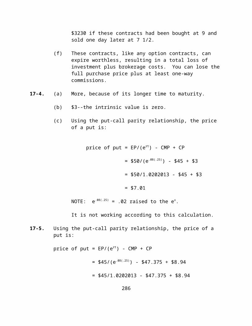
InvestmentReceipts
Legal/ Government by ERISA "Prudent Man" RuleRegulatory(Federal)Applies (State)
Unique Needs Cash Flow Reinvested; Widow's Needs And Are Immediate Circumstances And Govern
Now;Children’s Needs Should Be Considered in Planning for future
CFA21-11.
A. A useful framework that identifies and organizes the required inputs to an investment policy statement is the following:
Objectives Constraints
Return requirement Liquidity needsRisk tolerance Time horizon Tax
considerations Legal and regulatory considerations Unique needs, circumstances and preferences
B. The returns of a well-diversified portfolio (within an asset class) are highly correlated with the returns of the asset class itself. Over time, diversified portfolios of securities within an asset class tend to produce similar returns. In contrast, returns between different asset classes are often much less correlated, and over time, different asset classes are very likely to produce
323
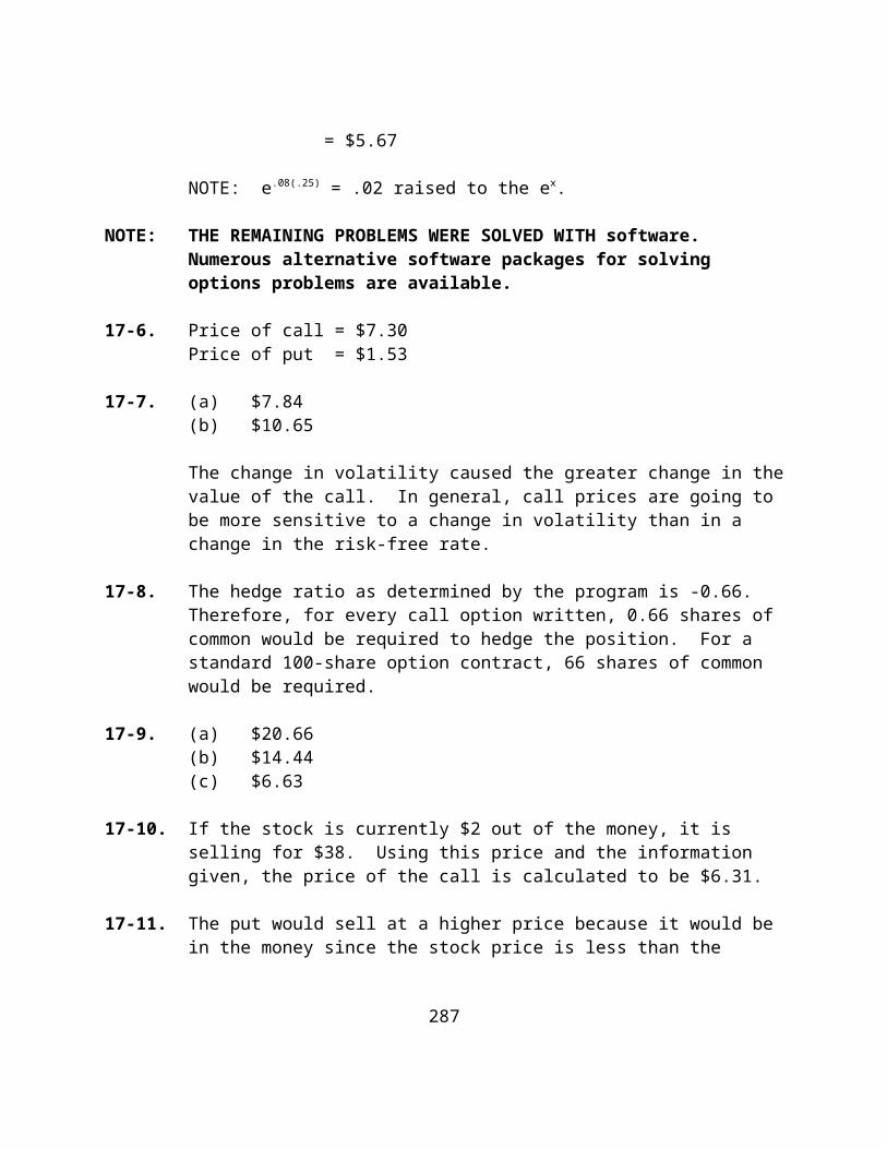
quite different returns. This expected difference in returns arising from differences in asset class exposures (i.e., from differences in asset allocation) is, thus, the key performance variable.
C. Three reasons why successful implementation of asset allocation decisions is more difficult in practice than in theory are:
(1) Transaction costs - investing or rebalancing a portfolio to reflect a chosen asset allocation is not cost-free; expected benefits are reduced by the costs of implementation.
(2) Changes in Economic and Market Factors - changing economic backgrounds, changing market price levels and changing relationships within and across asset classes all act to reduce the optimality of a given allocation decision and to create requirements for eventual rebalancing. Changes in economic and market factors change the expected risk/reward relationships of the allocation on a continuing basis.
(3) Changes in Investor Factors - the passage of time often gives rise to changes in investors needs, circumstances or preferences which, in turn, give rise to the need to reallocate, with the attendant costs of doing so.
In summary, even the “perfect” asset allocation is altered by the very act of implementation, due to transaction costs and/or changes in the original economic/market conditions and, as time passes, changes in the investor’s situation. These impediments to successful implementation are inherent in the process, mandating ongoing monitoring of the relevant input factors. In practice, the fact of change in one or more of these factors is a “given;” constant attention of the degree and the importance of the effects is required.
324

CFA21-12.
A. The investment process itself is common to all managers everywhere. Systematic exploitation of this underlying reality is as readily accomplished at a one-manager shop in which a hand-held calculator is used as it is by an industry giant employing the latest in real-time, on-line, interactive computer systems. The dynamic is there, and it is useful and fundamental.
The four key steps in the portfolio management process are:
1. Identify and specify the investor's objectives, preferences and constraints in order to develop explicit investment policies.
2. Develop and implement strategies through the choice of optimal combinations of financial and real assets in the marketplace.
3. Monitor market conditions, relative asset values and the investor's circumstances.
4. Make portfolio adjustments as appropriate to reflect significant changes in any or all of the relevant variables.
Portfolio management is a dynamic and continuous process with the four steps repeated again and again.
B. Objectives
Risk: While a need exists to protect both the corpus and the income stream against inflation, the Board of Trustees is “conservative” and spending needs are continuous while gift income is quite variable. These circumstances argue for adoption of a non-aggressive, medium-risk policy posture.
325
Return: Current income production of adequate proportions is clearly of major importance here, mitigated to some extent by the historical availability of gift supplements to endowment returns. A “spending rule” should be formulated by the Board that takes inflation into account, and policy should state a preference for income over gain without, however, adopting an extreme income orientation.
Constraints
Time Horizon: The actual horizon is clearly a very long one (perpetual, in concept) but given the nature of the objectives it would be useful if the policy statement spoke of, say, successive 5-year planning horizons with some fairly definite 1-year sub-goals.
LiquidityNeeds Since gifts are important but are quite
a variable as well, a 12-18 month liquidity reserve would be appropriate here to provide for spending continuity and possibly emergency needs. The existence of such a reserve might allow the Board to be a bit more aggressive in its asset allocation overall.
TaxConsiderations: Aside from meeting whatever Federal and
State reporting requirements may exist, taxes are a very minor matter here and
should have no effect on investment policy.
Legal &RegulatoryRequirements: Except for required conformity with the
Prudent Man Rule relating to
326
investments, and to any human-rights type regulations that may impact policy, these considerations are minor in this case. The policy statement may wish to give some specific attention to proxy-voting and like matters.
Unique Needs &Circumstances: The need to satisfy a conservative Board
and the wide variations in gift income must be addressed in whatever policy statement is produced. These are easily accommodated, however, and should not disrupt normal investment action.
CFA21-13.
A. Policy statement. An investment policy statement for the Foote family is as follows: “The Foote account should be invested to achieve maximum after-tax, inflation-adjusted, total return subject to their risk profile. Their substantial ability to tolerate risk is increased by the long time horizon and the absence of any need for liquidity. The tax implications favor focusing on long-term appreciation.”
Using the objectives constraints template, relevant policy considerations would include the following:
. Risk tolerance: high Return objectives:high - maximum
. Time horizon: long Taxes: important
. Liquidity needs: small Legal: observance of appropriate law
Justification. The Footes have said they do not expect to use the income or principal of the fund before their retirement, which is at least 30 years in the future. With such a long time horizon, they have a maximum ability to accept uncertainty of
327

returns and should seek the highest return given this high risk tolerance. The return focus should be “total” with an after-tax inflation-adjusted emphasis. The Footes do not need liquidity, and the couple does not have any truly unique limitations that would impose constraints on investment policy.
The interests of the charitable remainder do not conflict with those of the Footes and should not constrain the policy developed above. With significant passage of time or major changes in client circumstances, a policy adjustment might be necessary, but not at this point.
B. The expected versus required returns of the three funds as determined by the security market line are as follows:
Expected RequiredFund A 16.5% 17.6%Fund B 13.0% 12.8%Fund C 8.0% 8.0%
Determining an appropriate allocation for the Foote family requires considering both the security market line and the policy findings in Part A. The policy statement in Part A found the couple could tolerate high risk and therefore could accept the higher betas of Funds A and B. However, the required returns of the security market line must be determined to make a judgment about the propriety of each fund.
As the table above shows, Fund A is an inefficient portfolio because the expected returns are less than the required returns. Fund B would be a better choice considering only the security market line (SML). If taxes are considered and capital gains remain unrealized, Fund A’s after-tax rate of return would be 16.1 percent and Fund B's after-tax rate of return would be 11.8 percent. Taxes widen the return spread between A and B to 4.3 percent and can be used to justify the inclusion of Fund A. Because Fund B has 3 percent of its total 13 percent return from dividends, which are taxed at
328
40 percent, the after-tax expected return in Fund B drops from 13 percent to 11.8 percent.
A portfolio that uses more than one of the available funds should still have a growth orientation. The use of Fund C can be justified only by diversification or risk reduction and should be minimal given the high risk/high return policy objectives.
C. The $350,000 inheritance is expected to achieve a 12 percent rate of return, or $42,000, from its investment in the small-capitalization portfolio. The improved return from leverage would be the difference between the expected return, 12 percent, and the cost of borrowing, 8 percent, or 4 percent multiplied by the incremental funds, $150,000, or $6,000. The leverage would improve the total expected return from the portfolio and would, of course, impart additional risk to the portfolio.
D. The borrowing is appropriate based upon the policy statement in Part A. The fund has no liquidity needs and can accept the volatility implicit in a 1.4 beta because of the long time horizon.
CFA21-14.
A. A policy statement for the Hope Ministries would read: “The Foundation’s assets should be invested in keeping with the special requirements of its Charter and fiduciary laws to produce $90,000 of current income. Because of the perpetual nature of the Foundation, consideration should be given to protecting the value of the fund and the value of the future income stream from the effects of inflation. Moderate risk may be tolerated to achieve these objectives. Only minimal liquidity is required and taxes are of no concern.”
Using the objectives and constraints template, the following justification would be appropriate:
Return objectives: $90,000 in current income and appreciation of income and
329

asset value sufficient to offset expected inflation.
Risk tolerance: Moderate because the time horizon is long and inflation poses a potential threat over time.
Taxes: Tax exempt.
Legal constraints: Include the terms of the Charter, which require all income to be distributed and all appreciation, realized or not, to be retained (making a total return approach inappropriate), and the normal requirements of fiduciary law.
Liquidity: Not a major factor.
Unique factors: The Charter requirements mentioned above are relatively unique.
B. Fund B and C
A minimum of $90,000 in income must be achieved under any acceptable allocation. Because the Foundation can tolerate moderate risk, Omega could allocate $1,500,000 between Fund B and Fund C. For example, by investing $900,000 of the assets in Fund C, the Foundation receives $72,000 (8% x $900,000) of current income toward the required $90,000 annual income. Investing the remaining $600,000 in Fund B, which is also an efficient portfolio, produces income of $18,000, (3% x $600,000). This allocation produces the required $90,000 of income and would appreciate at a rate of $60,000 annually (10% x $600,000). Therefore, if Omega expects inflation to exceed 2%, this allocation ($900,000 to Fund C and $600,000 to Fund
330
B) would provide inflation protection up to 4% ($60,000/$1,500,000).
Undesirable AllocationsAllocating the endowment funds between U.S. Treasury bills and Fund C would lower the return and also lower the risk. This approach is not allowed by the question and is not recommended because the Foundation can tolerate a higher level of risk than provided by such an allocation.
Investing the entire amount in U.S. Treasury bills, Fund A or Fund B would not achieve the Foundation's objective of earning $90,000 in annual income.
. Treasury bills would provide only $60,000 (4% x $1,500,000) in annual income.
. Fund A would provide only $15,000 (1% x $1,500,000) in annual income.
. Fund B would provide only $45,000 (3% x $1,500,000) in annual income.
Fund A is an inefficient portfolio because the required return is 17.6% ([RA = 4% + 1.7 (12% - 4%)]) but its expected return is 16.5 percent. Therefore, Omega should avoid allocating funds to this inefficient portfolio.
Investing the entire portfolio in Fund C would provide no inflation protection because all of the income must be distributed for operations.
331
Chapter 22: Evaluation of Investment Performance
CHAPTER OVERVIEW
This chapter, which is concerned with measuring portfolio performance, is a logical concluding chapter for an investments text. The bottom line of investing for investors is deciding how well their portfolio performed and if they need to make changes.
Chapter 22 is a typical chapter in this area, covering the composite measures of portfolio performance as well as some of the newer concepts such as performance attribution. Although the composite measures have some problems, there is nothing better that is widely accepted, these measures are often seen and used in both textbooks and in the popular press, and they are easy to understand.
The chapter begins with a discussion of what is involved in evaluating portfolio performance, including the need to adjust for differential risk and differential time periods, the need for a benchmark, and constraints on portfolio managers. It also considers the difference between the portfolio’s performance and the manager's performance.
Included in the discussion is an outline of AIMR’s presentation standards, which likely will have a major impact in this area. These are minimum standards for presenting investment performance. These standards are being widely adopted by investment management firms.
The dollar-weighted and time-weighted returns measures are described, and the issue of risk is considered.
For expositional and other purposes at this level, the discussion centers around the three well-known risk-adjusted
332

(composite) measures of portfolio performance: Sharpe, Treynor and Jensen. Each of these is developed and illustrated separately. Actual mutual fund data is used to show how the measures are computed and evaluated. Additional discussion involves a comparison of the measures to each other, such as how the Sharpe and Treynor measures compare.
Along with the discussion of the measures themselves is related discussion of such issues as how to measure diversification. Also, capital market issues related to Jensen's measure are considered.
The chapter next considers the problems with portfolio measurement. This remains an unsettled issue in investments, with people using different measures and techniques, different benchmarks, and so forth. Students should be made aware that there is no standardized, widely accepted approach to this problem.
The chapter concludes with other issues in performance evaluation. Performance attribution is briefly considered.
CHAPTER OBJECTIVES
To outline the issues involved in measuring portfolio performance, including the problems that remain.
To present AIMR’s new presentation standards, and develop well-known measures of return consistent with these standards.
To develop and illustrate the three composite measures of portfolio performance.
To consider other important issues, such as performance attribution.
333
MAJOR CHAPTER HEADINGS [Contents]
Framework for Evaluating Portfolio Performance
Some Obvious Factors to Consider[differential risk levels; differential time periods; appropriate benchmarks; constraints on portfolio managers; other considerations]
AIMR’s Presentation Standards[outline of some of the minimum standards for presenting investment performance]
Return and Risk Considerations
Measures of Return[Total Return; dollar-weighted return; time-weighted return]
Risk Measures[total risk; nondiversifiable risk]
Risk-Adjusted Measures of Performance
The Sharpe Performance Measure[equation; diagram; example with mutual fund data]
The Treynor Performance Measure[equation; diagram; example with mutual fund data; comparing the Sharpe and Treynor Measures; measuring diversification]
Jensen’s Differential Return Measure[development of equation; diagram; how to use; significance; a comparison of the three composite measures]
Problems With Portfolio Measurement
[Roll’s arguments about beta; benchmark error; other problems]
Other Issues In Performance Evaluation
334
Monitoring Performance
Performance Attribution[definition; issues; bogey]
Can Performance Be Predicted?
POINTS TO NOTE ABOUT CHAPTER 22
Tables and Figures
Table 22-1 is an outline of AIMR’s Performance Presentation Standards. These standards are discussed at various points in the chapter.
Table 22-2 contains the mutual fund data discussed in the chapter. As such, it is for informational purposes in illustrating the calculations of the composite measures, the measure of diversification, and so forth.
Table 22-3 shows the risk-adjusted measures for the five equity mutual funds used in the analysis of the risk-adjusted measures.
The figures in this chapter are standard figures showing the three measures of composite performance and characteristic lines. They are keyed to discussion in the text in terms of the mutual fund data used, but otherwise there is nothing unique about them. Instructors can easily use comparable figures of their own to illustrate the major points about the composite measures of performance.
Figure 22-1 shows Sharpe’s measure of performance for five mutual fund portfolios, with three funds plotting above the CML and two below.
Figure 22-2 shows Treynor’s measure of performance for three mutual fund portfolios, with three of these funds plotting above the SML and two below.
Figure 22-3 illustrates Jensen’s measure of portfolio performance for three hypothetical funds.
335
Box Inserts
There are no box inserts for this chapter.
336
ANSWERS TO END-OF-CHAPTER QUESTIONS
22-1. The framework for evaluating portfolio performance primarily involves an analysis of both the returns and the risk of the portfolio being evaluated and a comparison to a proper benchmark. Other issues include the diversification of the portfolio and an evaluation of the manager as opposed to the portfolio itself.
22-2. It is important to determine if a portfolio manager is following the stated objectives for the portfolio. It is also necessary to analyze any constraints imposed on a portfolio manager. If a portfolio outperforms its expected benchmark, such results may be attributable to the manager. If the portfolio manager ceases to manage this portfolio, potential investors will want to be aware of this fact.
22-3. The three composite measures use either standard deviation (from the CML) or beta (from the SML) as a risk measure. It is easy to see how Jensen’s measure is directly related to the CAPM. There is a derivable relationship between Jensen's measure and Treynor’s measure, thereby connecting Treynor’s measure to the CAPM. Finally, Sharpe’s measure can be related to capital market theory.
22-4. The Sharpe measure takes into account how well diversified the portfolio was during the measurement period. Any difference in rankings between the two measures should reflect the lack of diversification in the portfolio. With perfect diversification, the two measures produce identical rankings.
22-5. Regressing a portfolio’s returns against the market’s returns for some period of time results in a characteristic line for the portfolio. Such a line shows the linear relationship between the fund’s returns and the market’s returns; that is, it shows how well the former is explained by the latter.
22-6. Portfolio diversification can be measured by the coefficient of determination (R2), which is produced when a characteristic line is fitted. If the fund is totally diversified, the R2 will approach 1.0, indicating that
the fund’s returns are completely explained by the market’s returns. On average, mutual funds have high degrees of diversification (i.e., an R2 of .85 or .90, or higher).
22-7. An index fund should show complete diversification.
22-8. Investors who have all (or substantially all) of their assets in a portfolio of securities should rely more on the Sharpe measure because total risk is important.
For investors whose portfolio constitutes only one part of their total assets, systematic risk is the relevant risk and the Treynor measure would be appropriate.
22-9. Start with the CAPM equation, using a portfolio subscript p. If investor’s expectations are, on average, fulfilled, the equation can be approximated ex post as:
Rpt = RFt + bp[Rmt-RFt] + Ept (22-5)
Rearranging,
Rpt - RFt = bp[Rmt-RFt] + Ept (22-6)
Finally, an intercept term, alpha, can be added to 22-6 to identify superior or inferior portfolio performance.
22-10. The Jensen measure is computationally efficient because the beta for the portfolio is estimated simultaneously with the alpha, or performance measure.
22-11. The alpha must be statistically significant to be meaningful. If it is not significantly different from zero, it doesn’t mean much, whether positive or negative.
22-12. Roll has argued that no unambiguous test of the CAPM has yet been conducted. Since the composite performance measures are based on the CAPM (or capital market theory), they are also called into question.
22-13. The use of different market indices can result in different betas for a portfolio. This, in turn, could lead to different rankings for a portfolio; that is, if a “wrong” market index was used, a portfolio could rank lower than it otherwise would.
22-14. In theory, the proper market index to use would be the “true” market portfolio--the portfolio of all risky
assets, both financial and real, in their proper proportions. Such a portfolio is completely diversified.
22-15. The steeper the angle, the higher the slope of the line, and the better the performance. A portfolio with a line steeper than that of the market has outperformed the market.
22-16. No. Sharpe and Jensen use different measures of risk, and different procedures; therefore, different rankings of performance can be obtained.
22-17. b
22-18. b
22-19. c

ANSWERS TO END-OF-CHAPTER PROBLEMS
22-1. (a) The RVAR are:
Fund Rank 1 (14-6)/21 = .38 fourth 2 (16-6)/21 = .48 second 3 (26-6)/30 = .67 first 4 (17-6)/25 = .44 third 5 (10-6)/18 = .22 fifthMarket (12-6)/20 = .30
(b) The RVOL are:
Fund Rank 1 (14-6)/1.15 = 6.96 fifth 2 (16-6)/1.10 = 9.09 third 3 (26-6)/1.30 = 15.38 first 4 (17-6)/ .90 = 12.22 second 5 (10-6)/ .45 = 8.89 fourthMarket (12-6)/1.00 = 6.00
(c) Yes, there are differences. Note that the numerator values for the RVAR are exactly the same as for the RVOL. The differences arise from the differences in risk as measured by the SD and the beta. The difference in rankings is caused by the degree of diversification.
(d) For the RVAR, only Fund 5 failed to outperform the market. For the RVOL, all of the funds outperformed the market.
22-2. (a) Fund 1. It has the highest R2.
(b) Standard deviations are needed to answer this question.
(c) Fund 4 has the lowest market risk, and fund 5 is the highest.
(d) Funds 2 and 5 are the only funds with alphas that are positive and statistically different from zero.
22-3. (a) The RVAR are:
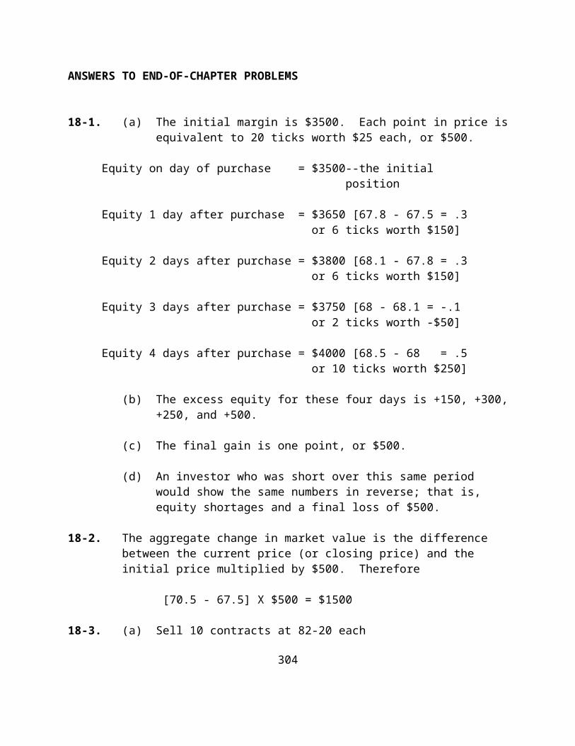
Fund Rank
A (17.0-8.6)/20.0 = .42 fifth (5) B (19.0-8.6)/17.8 = .584 first (1) C (12.3-8.6)/25.0 = .15 tenth (10) D (20.0-8.6)/24.5 = .47 fourth (4) E (15.0-8.6)/17.4 = .37 sixth (6) F (19.0-8.6)/18.0 = .578 second (2) G ( 8.6-8.6)/19.0 = 0.0 eleventh (11) H (20.0-8.6)/21.5 = .53 third (3)
Market (11.0-8.6)/20.5 = .117
(For some of the funds, the RVAR are shown to an additional number of decimal places in order to eliminate ties).
(b) The RVOL are:
Fund Rank
A (17.0-8.6)/ .88 = 9.545 fifth (5)B (19.0-8.6)/ .65 = 16.000 first (1) highC (12.3-8.6)/ .83 = 4.478 ninth (9)*D (20.0-8.6)/1.00 = 11.400 fourth (4) E (15.0-8.6)/ .79 = 8.101 sixth (6)F (19.0-8.6)/ .83 = 12.530 second (2)G ( 8.6-8.6)/ .91 = 0.0 eleventh (11) lowH (20.0-8.6)/ .93 = 12.258 third (3)
Market (11.0-8.6)/1.00 = 2.40
(* = ranking by RVOL different from that of RVAR.)
(c) The highest R2 (the greatest diversification) is for Fund G, the lowest is for Fund C. Except for Funds B and C, it appears that the funds are highly diversified.
(d) Funds F and H have positive alphas (and positive t values greater than 2.365), and therefore have above average performance.

(e) betas alphas
excess original excess excess original excess - orig. - orig.
A .87 .88 -.01 6.57 7.53 - .96 B .61 .65 -.04 8.81 11.70 -2.89 C .86 .83 +.03 1.58 7.53 -1.54 D 1.03 1.00 +.03 8.98 3.12 - .02 E .81 .79 +.02 4.34 6.15 -1.81 F .83 .83 0.0 8.69 10.11 -1.42 G .92 .91 +.01 -2.22 -1.37 - .85 H .95 .93 +.02 8.88 9.52 - .64
Using the [excess-original] beta differences, two betas are less, one unchanged, and five are larger. No generalization about larger or smaller betas is possible because it depends on the relative covariance of RF with the market return and the covariance of RF with the portfolio return. Therefore, the betas using excess returns may be greater or smaller than the betas with the original returns.
With the alpha differences [excess-original], all are negative, but the magnitudes vary widely. This is somewhat illusory, because no beta is greater than unity. If we had used a constant for RF (the average RF for the period) then the betas above would have not been equal to the excess betas, and:
excess alpha = [RF(ß-1) + original alpha]
So, for portfolios with betas less than unity, the excess alpha is smaller; and for portfolios with betas greater than unity, the excess alpha is larger.
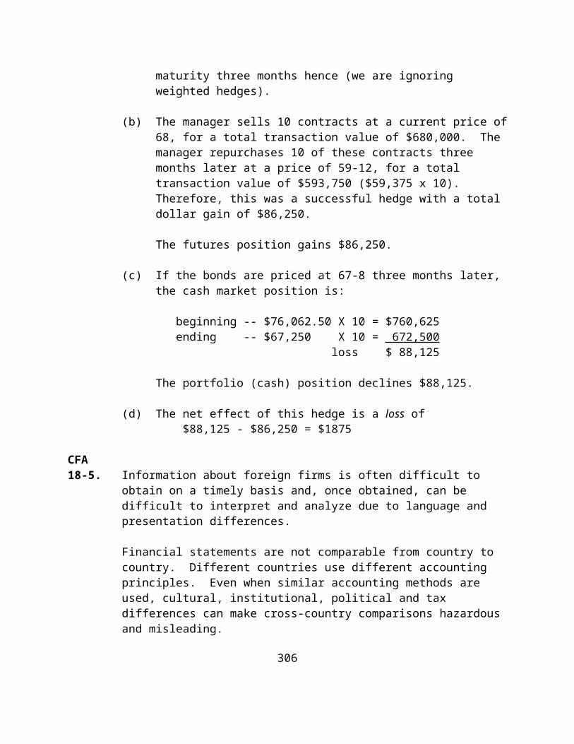
22-4. Using the data as given in the problem, the results are as follows:
Market Return RF Portfolio 1 Portfolio 2
Mean 8.0 7.6 10.3 9.9SD 13.3 - 15.8 17.12Beta 1.0 - 1.15 1.24R2 1.0 - 0.93 0.93RVAR 0.03 - 0.17 0.13RVOL 0.40 - 2.35 1.85Alpha 0.00 - 2.24 1.80
Based on these results, the answers are as follows:
(a) portfolio 1 ranks higher
(b) portfolio 1 ranks higher
(c) portfolio 1 has the higher alpha
(d) since the R2 is the same for each, unsystematic risk is a tie
(e) portfolio 2 has the larger beta
(f) portfolio 2 has the larger standard deviation
(g) portfolio 1 has the larger mean return
(h) portfolio 1 has a larger mean return but a smaller SD and beta compared to portfolio 2. The result is a larger RVAR and RVOL.
22-5. (a) portfolio 3 has the widest range of returns and the largest beta
(b) portfolio 3 for the same reason
(c) portfolio 1’s returns are closest to the market, and therefore best explained by the market
(d) there is no way to be certain without doing the calculations
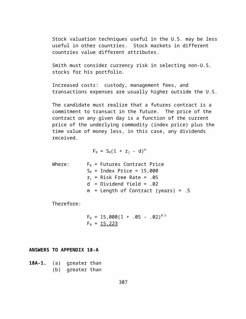
(e) the results using the data as given are as follows:
Market Portfolio Portfolio Portfolio Return RF 1 2 3
Mean 12.33 7.17 16.33 17.15 15.17SD 12.36 - 12.63 13.55 18.5Beta 1.0 - 1.00 1.06 1.35R2 1.0 - 0.96 0.94 0.81RVAR 0.42 - 0.73 0.76 0.43RVOL 5.17 - 9.17 9.73 5.93Alpha 0.00 - 4.00 4.84 1.03
Based on this, the portfolios rank as follows:
on RVAR: 2, 1, 3on RVOL: 2, 1, 3
(f) on R2, the portfolios rank 1, 2, 3
(g) portfolio 2 had the largest alpha
(h) portfolio 2, using composite measures
22-6. (a) portfolio 1 has returns identical to the market and a beta of 1.0
(b) portfolio 2 has returns exactly twice those of the market, and a beta of 2.0
(c) the R2 is going to be 1.0 in each case because the market returns will explain each portfolio’s returns perfectly
(d) the market has an alpha of zero, so portfolio 1 does also
(e) it would have to be identical since the returns are the same
CFA22-7. a
CFA22-8. d

CFA22-9. a
CFA22-10. c
CFA22-11. A. The Treynor measure (T) relates the rate of return
earned above the risk-free rate to the portfolio beta during the period under consideration. Therefore, the Treynor measure shows the risk premium (excess return) earned per unit of systematic risk:
Ri-Rf
Ti = ─────, i
whereRi = average rate of return for portfolio i
during the specified period,
Rf = average rate of return on a risk-free investment during the specified period, and
i = beta of portfolio i during the specified period.
Performance Relative Treynor Measure to the Market (S&P 55)
10%-6% T = ────── = 6.7% Outperformed 0.60
Market (S&P 500)
12%-6% TM = ────── = 6.0%
1.00
T examines portfolio performance in relation to the security market line (SML). Because the portfolio would plot above the SML, it outperformed the S&P 500 Index. Because T was greater than TM, 6.7 percent versus 6.0 percent, respectively, the portfolio clearly outperformed the market index.
The Sharpe measure (S) relates the rate of return earned above the risk free rate to the total risk of a portfolio by including the standard deviation of returns. Therefore, the Sharpe measure indicates the risk premium (excess return) per unit of total risk:
Ri-Rf
Si = ─────, i
Ri = average rate of return for portfolio i during the specified period,
Rf = average rate of return on a risk-free investment during the specified period, and
i = standard deviation of the rate of return for portfolio i during the period.
Performance Relative Sharpe Measure to the Market (S&P 500)
10%-6% S = ────── = 0.222 Underperformed 18%
Market (S&P 500)
12%-6% SM = ────── = 0.462 13%
The Sharpe measure uses total risk to compare portfolios with the capital market line (CML). The portfolio would plot below the CML, indicating that it under-performed the market. Because S was less than SM, 0.222 versus 0.462, respectively, the portfolio under-performed the market.
B. The Treynor measure assumes that the appropriate risk measure for a portfolio is its systematic risk, or beta. Hence, the Treynor measure implicitly assumes that the portfolio being measured is fully diversified. The Sharpe measure is similar to the Treynor measure except that the excess return on a portfolio is divided by the standard deviation of the portfolio.
For perfectly diversified portfolios (that is, those without any unsystematic or specific risk), the Treynor and Sharpe measures would give consistent results relative to the market index because the total variance of the portfolio would be the same as its systematic variance (beta). A poorly diversified portfolio could show better performance relative to the market if the Treynor measure is used but lower performance relative to the market if the Sharpe measure is used. Any difference between the two measures relative to the markets would come directly from a difference in diversification.
In particular, Portfolio X outperformed the market if measured by the Treynor measure but did not perform as well as the market using the Sharpe measure. The reason is that Portfolio X has a large amount of unsystematic risk. Such risk is not a factor in determining the value of the Treynor measure for the portfolio, because the Treynor measure considers only systematic risk. The Sharpe measure, however, considers total risk (that is, both systematic and unsystematic risk). Portfolio X, which has a low amount of systematic risk, could have a high amount of total risk, because of its lack of

diversification. Hence, Portfolio X would have a high Treynor measure (because of low systematic risk) and a low Sharpe measure (because of high total risk).