investment in australian aboriginal art

1

Investment in Australian Aboriginal Art

Jenny Lye and Joe Hirschberg1

October 2020

Abstract

Recent changes in Australian legislation that limit the value of how artworks that can be considered as assets in retirement funds have had an impact on the Australian Aboriginal Art market. In this paper we estimate the impact of these changes on the price index based on prices paid for 15,845 works by over 200 artists at art auctions from 1986 to 2019.

Using an OLS and a quantile regression approach, we estimate hedonic price models for various segments of the Australian Aboriginal art market. These models are used to estimate price indices in order to investigate if the changes in Australian laws concerning the sale and use of art assets has influenced the potential returns for different segments of the market.

Key words: resale royalties, art market price index, segmented price index, restrictions on assets for retirement funds

1 Department of Economics, University of Melbourne, Melbourne 3010, AUSTRALIA.

2

Contents

1: Introduction ............................................................................................................................. 3

2: Australian Aboriginal Art (AAA). ............................................................................................... 4

3: Factors Affecting the AAA Market .......................................................................................... 7

3:a 2018 Changes to the Protection of the Moveable Cultural Heritage Act 1986 (PMCH) .... 7

3:b Indigenous Australian Art Commercial Code of Conduct .................................................. 8

3:c Global Financial Crisis (GFC) ............................................................................................ 8

3:d Resale Royalty Scheme (RRS) – June 2010 ....................................................................... 8

3:e Changes to self-managed superannuation funds July 2011 – July 2016 ............................. 9

4: The Hedonic Price ndex Model ................................................................................................ 11

5: Estimation Results and the Art Index.................................................................................... 16

5:1 Estimating the Average Art Index using the OLS Model ................................................. 16

5:2 The Quantile Art Index ..................................................................................................... 19

6: Discussion ............................................................................................................................. 28

References ......................................................................................................................................... 30

Appendix Estimated Coefficient plots ........................................................................................... 32

Figure A.1 The year indicator variables ....................................................................................... 32

Table A.2 The Auction House Indicator Variables ...................................................................... 34

Figure A.3 The Repeat sales, Sold out of Australia, Sold after death and Telstra Awards Indicator Variables ........................................................................................................................ 36

Figure A.4 The Artist Specific Indicator Variables ..................................................................... 37

3

1: Introduction

In the past 10 years fine art has increasingly become an alternative investment asset

for more than just high net wealth individuals. The Luxembourg office of the Deloitte

consulting firm has promoted the consideration of art as financial asset in conjunction with

more traditional assets such as equites, bonds, real estate and precious metals in a series of

special reports on this alternative since 2011 (Deloitte and ArtTatic 2019). The increases in

value of some portfolios of fine art have been measured as appreciating faster than many

alternative traditional assets Etro and Stepanov (2019). The most recent estimate of the

private holdings of art and collectables has been estimated as US$1.742 trillion (page 27

Deloitte and ArtTatic 2019). In 2019 it has been estimated that global sales of art were

US$64.1 billion (page 1, McAndrew 2020) and since 2000 the increase in the price index for

contemporary art has been approximately 300% (Etro and Stepanov 2019).

The increased volume in the fine art market has attracted a greater degree of

government regulation. In this paper we investigate the extent to which the sales of

Australian Aboriginal Art (AAA) may have been influenced by the introduction of legislation

in Australia. This legislation has changed three factors in the sale of AAA. First, the

conditions under which it can be considered as an investment asset. Second, that removal

from Australia may be limited when classified as cultural heritage. And third, that they are

subject to royalty payments when resold.

The rest of the paper proceeds as follows. First, we provide a brief description of the

rise of the contemporary AAA. Then, we provide a background of the current market in AAA

and the legislative actions that may have had an influence on the recent sales pattern. We

then describe the hedonic price model we specify to account for characteristics of the art that

can influence its sale price. We also include indicators for the dates when changes in

legislation occur to determine if they have had a measurable influence on the sale price. We

estimate this model with both the least-squares and quantile methods. The quantile approach

allows us to accommodate different segments of the market and because of the wide variation

in the prices of artworks in the sample. We compare the estimated price indices with the

returns from traditional stock indices and the price indices that have been produced for the

international market in contemporary art to determine how the market for AAA compares.

The final section presents conclusions and caveats to the results.

4

2: Australian Aboriginal Art (AAA).

All Aboriginal societies share similar creation stories often referred to as ‘the

dreaming’ or ‘the dreamtime’. These explain the origin of the universe and the purpose of

everything in it. Art is used to pass knowledge down through the generations. Initially these

were depicted on rock walls, the body and in the sand. The present-day artwork on bark,

canvas and board only commenced around 50 years ago. Aboriginal Artists need permission

to paint particular stories and inherit the rights to these stories which are passed down

through generations within certain skin groups. An Aboriginal artist cannot paint a story that

does not belong to their clan. As Michael Nelson Tjakamarra, one of the well-known desert

painters said, “Without the story the painting is nothing” (Genocchio 2008 pg. 96). Many

women artists for example, paint stories associated with finding bush tucker such as bush

potatoes, bush cabbage, honey ants and wild yams since women are the traditional principal

food gatherers.

Until the 1970s Indigenous art was largely of ethnographic interest (Acker 2016).

However, during the 1970s the beginnings of a commercial art market began and now for

many residents of remote Indigenous Australian communities' art production is the principal

non-welfare source of income. Typically, the artist's first or primary sale is through an agent

whereas subsequent or secondary sales are most predominantly through an auction house.

Only since the mid-1990s has there been a substantial secondary market for Aboriginal

artwork (Genocchio 2008 pg 214). Primary and secondary markets are intricately linked as

collectors are unlikely to spend significant amounts of money in the primary market if the

artist does not have an established auction market. The most expensive Aboriginal artwork

ever sold at auction was Clifford Possum Tjapaltjarri’s painting Warlugulong (1977)2 selling

for $2.4 million in 2007.3 Prior to this it had been sold at auction in 1996 for $39,200.

Originally, Clifford Possum Tjapaltjarri sold Warlugulong (1977) for $1,200 to a small art

gallery where it was later bought by a bank and for twenty years it was hung in their

cafeteria.4 Two months earlier in 2007, Emily Kame Kngwarreye’s painting Earth’s Creation

2 It is quite common for Aboriginal Artists to name multiple work with the same name thus it is often necessary to use either numbering or dates to distinguish them. 3 Unless otherwise noted the $ amounts listed in this paper are in Australian dollars of the time. Note that for the period from 1987 to 2019 the average purchasing power parity rate was $US .73 to $AU 1.00. (OECD tables at https://data.oecd.org/conversion/purchasing-power-parities-ppp.htm.) 4 See https://www.reuters.com/article/us-australia-art/aboriginal-masterpiece-sets-new-art-record-idUSSYD16281320070725

5

I (1994) sold for $1.056 million and more recently in 2017 for $2.1 million. It is the most

expensive piece of art by an Australian woman ever sold.5

It has been suggested that the rise of the Aboriginal art market in Australia began in

the early 1980s, when museums began including the work in contemporary art shows. In

1981 the Art Gallery of New South Wales included work by Clifford Possum Tjapaltjarri and

Tim Leura Tjapaltjarri in the inaugural edition of “Australian Perspecta,” a biennial

exhibition of contemporary Australian art that ran through 1999.6 Other major exhibitions by

the Papunya Tula Artists have also drawn significant attention to Aboriginal art including the

display at the World Expo '88 in Brisbane and a major retrospective exhibition in Sydney to

coincide with the Sydney Olympics in 2000. The National Aboriginal and Torres Strait

Islander Art Award started in 1983 and has become a significant annual showcase of

contemporary Aboriginal art. Major exhibitions have also been held overseas. In 1988,

“Dreamings: The Art of Aboriginal Australia”, opened at the Asia Society in New York City

and later moved to the David and Alfred Smart Gallery of the University of Chicago. The

auction house Sotheby’s has promoted Indigenous art in the global market since launching its

stand-alone Aboriginal art auctions in 1997. In 1990, Rover Thomas and Trevor Nickolls

exhibited their work at the Venice Biennale followed by Emily Kame Kngwarreye, Yvonne

Koolmatrie and Judy Watson in 1997. In 2008 the exhibition Utopia: The Genius of Emily

Kame Kngwarreye attracted over 120,000 visitors to the National Museum of Art in Osaka

and the National Arts Center in Tokyo.7 In December 2019, Sotheby’s held the first New

York auction of Aboriginal contemporary art. The sale totaled US$2.8 million and the most

expensive painting sold was Emily Kame Kngwarreye’s painting Celebration (1991)

estimated at US$300,000 to US$400,000 and selling for US$596,000.8

There are many different styles of Australian Aboriginal art. Aboriginal bark painting

is a practice that goes back thousands of years and before the 1970s they were the most

identifiable form of Aboriginal art. Today they are mainly associated with Arnhem Land and

other regions in the Top End of Australia. The paintings can be drawn using different

mediums showing aspects of Aboriginal life and most carry the sign of the clan, essentially

naming the people responsible for the art. Cross hatching is often used and involves closely

spaced fine lines drawn in particular colours, intersecting each other. The chosen colours

5 See https://www.theguardian.com/artanddesign/2017/nov/17/emily-kame-kngwarreye-painting-sells-for-21m-in-sydney 6 See https://www.artsy.net/article/artsy-editorial-driving-rise-aboriginal-art-market 7 See https://japan.embassy.gov.au/tkyo/indigenousarts.html 8 See https://news.artnet.com/market/sothebys-new-york-first-aboriginal-sale-1733955

6

may be specific to a clan. As bark paintings can warp and change shape over time they tend

to not achieve as high a price as paintings on canvas.

Albert Namatjira was the most famous Aboriginal artists to work in a European style.

He captured Australia’s desert scenery in a European-watercolour style. He was born in 1902

and learnt to paint using watercolours while working as a ‘camel boy’ on painting exhibitions

to central Australia in the 1930s with the Australian artist Rex Battarbee. His landscapes

have now been evaluated as coded expressions on traditional sites and sacred knowledge.9

His style of work was adopted by other Indigenous artists in the region beginning with his

close male relatives, and they became known as the Hermannsburg School.

The ‘dot painting’ style originating in the early 1970s has become one of the

recognizable characteristics of Aboriginal art. An art teacher for the children in Papunya

helped Aboriginal artists transfer depictions of their stories from desert sand to flat surfaces.

However, the early paintings had few dots at all. Rather, they tended to be an accurate

cursive style representation of cultural traditions and sometimes depicted sacred objects and

secret information that was forbidden to be seen by the uninitiated. This provoked outrage

and anger within the desert Aboriginal community once these paintings began to sell outside

the settlement. The ‘dot painting’ style was developed to provide a more simplified

iconography that was less revealing (Gennocchio 2008). Originally colours were restricted to

variations of red, yellow, black and white produced from ochre, charcoal and pipe clay. Later

acrylic mediums were introduced allowing for more vivid colourful paintings.

While in the 1970s the painting movement was largely confined to Papunya it

developed rapidly in the 1980s. It is not a homogeneous entity. It differs in character and

style depending from which region the artist is from and what language is spoken. The usual

groupings are of art from the Central Australian desert; the Kimberley in Western Australia;

the northern regions of the Northern Territory, particularly Arnhem Land, and northern

Queensland, including the Torres Strait Islands.

Urban art is another distinct style of Indigenous art. This label emerged in the 1980s

and includes Aboriginal artists from all metropolitan centres and suburbs across Australia, as

opposed to Aboriginal artists living in rural or remote communities. These artists tend to

work in a wide range of media and often the works are statements on contemporary social

issues.

9 See https://www.artgallery.nsw.gov.au/collection/artists/namatjira-albert/

7

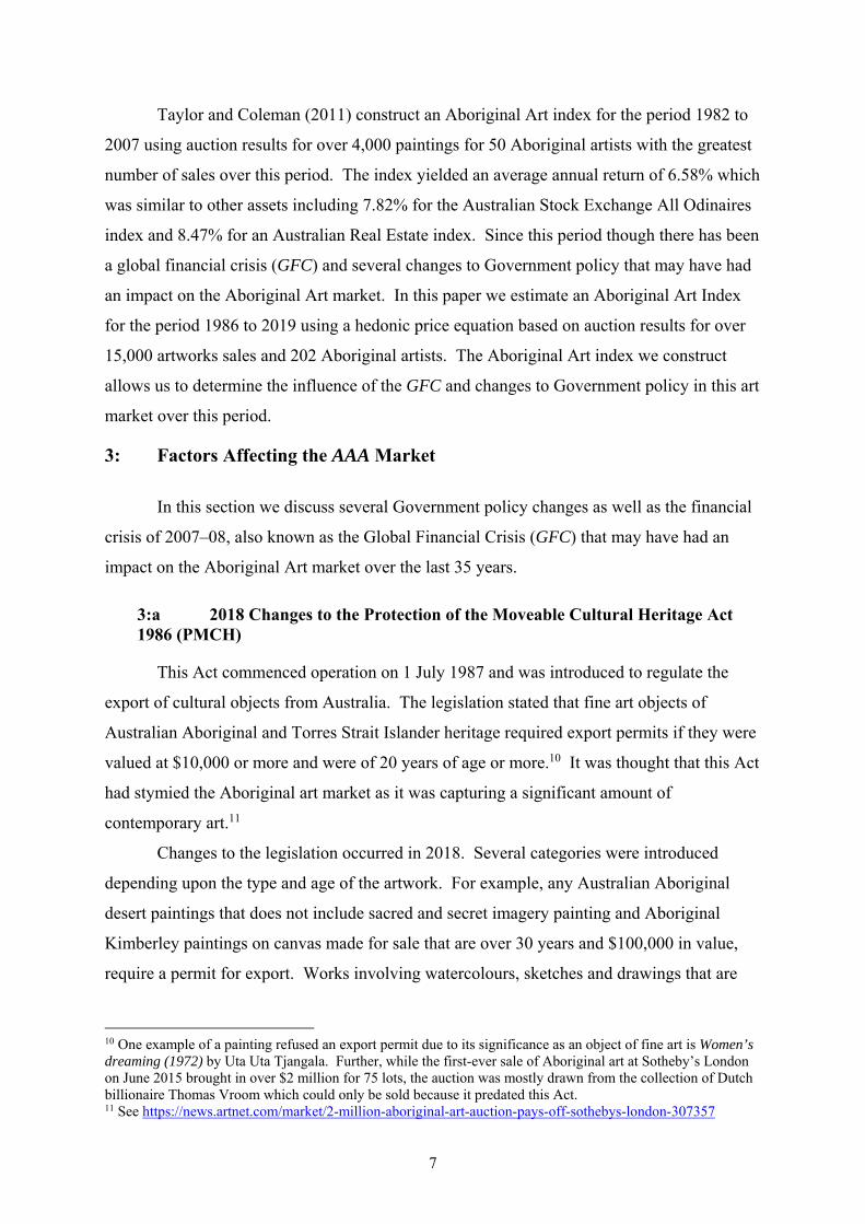
Taylor and Coleman (2011) construct an Aboriginal Art index for the period 1982 to

2007 using auction results for over 4,000 paintings for 50 Aboriginal artists with the greatest

number of sales over this period. The index yielded an average annual return of 6.58% which

was similar to other assets including 7.82% for the Australian Stock Exchange All Odinaires

index and 8.47% for an Australian Real Estate index. Since this period though there has been

a global financial crisis (GFC) and several changes to Government policy that may have had

an impact on the Aboriginal Art market. In this paper we estimate an Aboriginal Art Index

for the period 1986 to 2019 using a hedonic price equation based on auction results for over

15,000 artworks sales and 202 Aboriginal artists. The Aboriginal Art index we construct

allows us to determine the influence of the GFC and changes to Government policy in this art

market over this period.

3: Factors Affecting the AAA Market

In this section we discuss several Government policy changes as well as the financial

crisis of 2007–08, also known as the Global Financial Crisis (GFC) that may have had an

impact on the Aboriginal Art market over the last 35 years.

3:a 2018 Changes to the Protection of the Moveable Cultural Heritage Act 1986 (PMCH)

This Act commenced operation on 1 July 1987 and was introduced to regulate the

export of cultural objects from Australia. The legislation stated that fine art objects of

Australian Aboriginal and Torres Strait Islander heritage required export permits if they were

valued at $10,000 or more and were of 20 years of age or more.10 It was thought that this Act

had stymied the Aboriginal art market as it was capturing a significant amount of

contemporary art.11

Changes to the legislation occurred in 2018. Several categories were introduced

depending upon the type and age of the artwork. For example, any Australian Aboriginal

desert paintings that does not include sacred and secret imagery painting and Aboriginal

Kimberley paintings on canvas made for sale that are over 30 years and $100,000 in value,

require a permit for export. Works involving watercolours, sketches and drawings that are

10 One example of a painting refused an export permit due to its significance as an object of fine art is Women’s dreaming (1972) by Uta Uta Tjangala. Further, while the first-ever sale of Aboriginal art at Sotheby’s London on June 2015 brought in over $2 million for 75 lots, the auction was mostly drawn from the collection of Dutch billionaire Thomas Vroom which could only be sold because it predated this Act. 11 See https://news.artnet.com/market/2-million-aboriginal-art-auction-pays-off-sothebys-london-307357

8

over 30 years old and $40,000 in value require a permit as well as any Aboriginal acrylic

painting over $350,000 in value. Aboriginal or Torres Strait Islander ochre paintings that are

on bark, composition board, wood, cardboard, stone or other similar supports require a permit

if they are 30 years of age or more and valued at $20,000 or more. However, pre-1901

Aboriginal or Torres Strait Islander artworks valued at $25,000 or more and pre-1960

Aboriginal or Torres Strait Islander bark paintings or sculptures valued at $25,000 or more

cannot be exported out of Australia.12 The changes were designed to allow “decisions to be

made more quickly, cheaply, transparently, and certainly – while more effectively protecting

Australia’s most significant material” (Simpson 2015).

3:b Indigenous Australian Art Commercial Code of Conduct

The Code was officially launched on 29 November 2010 to specify a set of minimum

standards for dealers, agents and artists, and defined terms of trade and rights and

responsibilities for the sale and management of artworks. It is considered to not have had a

major impact on the market as registration to the code was voluntary.13

3:c Global Financial Crisis (GFC)

GFC refers to the period of between mid-2007 and early 2009. It “impacted on

people’s appetite for art and it became a luxury spend” (Lamont 2011). During this crisis the

global art market aggregate sales fell by over 37% when they went from US$62 billion in

2008 to US$39 billion in 2009. By 2018 sales global sales had recovered to US$67 billion

(see Solimano 2019).

Higgs (2012) constructed an art price index based on works from 71 well-established

Australian (including only 4 Indigenous) artists. She found this index was similar to the

Australian stock market with a downturn in the middle of 2008 corresponding to the GFC.

Further, she showed that during the GFC average art returns declined in nominal terms by

close to six per cent with a standard deviation of twenty-one per cent.

3:d Resale Royalty Scheme (RRS) – June 2010

A resale royalty scheme in Australia was established with the intention of giving

artists the right to receive a share in the financial profit from resales of their artworks. This

12 See https://www.greeradamsfineart.com/news/exporting-aboriginal-art 13 Details of the code can be found at https://indigenousartcode.org/the-indigenous-art-code/ and for a discussion on the impact see http://www.abc.net.au/worldtoday/content/2012/s3597288.htm

9

scheme was particularly important for Aboriginal artists who lived in poverty while their

artwork resold at high prices at auctions.

For example, Johnny Warangkula Tjupurrula (1925-2001) was a founding member of

the Papunya Tula painting movement. While in the early 1980s his paintings frequently sold

for $10,000 by the mid-1980s he developed cataracts affecting the quality of his artwork.

Most of the money he had made from the sales of his artwork he had given away to family

and in 2001 he died without any possessions. However, while his painting Water Dreaming

at Kalipinypa created in 1972 originally sold for $150, in 1997 it sold at auction for $206,000

and in 2000 for $486,500. He received none of the proceeds of these higher sales

(Gennocchio 2008).

The Resale Royalty Scheme came into effect on 9th June 2010. This scheme entitles

the artist to a 5% royalty of the sales price of the artwork when it resells commercially for

$1,000 or more although, the artist is required to satisfy a residency test and if they are

deceased the royalty is payable to beneficiaries who also meet the test. The royalty only

applies on works that are sold during the life of the artist or within 70 years following their

death. Between June 2010 – December 2019 more than $8 million dollars has been generated

for over 1,900 artists from 20,000 resales with most royalties being between $50 and $500.14

However, for auctions, Wilson-Anastasios (2019) reports that two market auction houses,

Deutscher and Hackett and Sotheby’s, that account for almost half of Australia’s auction

turnover collected less than $70,00 and $6,200 for Indigenous artists respectively. Further, it

has been suggested that auction houses may avoid the sale of low value transactions as a way

to minimize the administrative burden of the scheme (Challis 2019).

3:e Changes to self-managed superannuation funds July 2011 – July 2016

Due to the increased use of art as an investment, national governments have found it

necessary to codify the distinction between investment in art and collecting art in order to

establish how art sales are considered under tax legislation. For example, the United States

Internal Revenue Service (IRS) make a distinction for taxation purposes between the sale of

pieces of fine art as either part of a personal collection or as the inventory of a gallery. In

addition, the IRS does not allow investment in collectables to be considered in the portfolio

of an Individual Retirement Account (IRA).15

14 See www.resaleroyalty.org.au 15 See details at: https://www.irs.gov/retirement-plans/investments-in-collectibles-in-individually-directed-qualified-plan-accounts.

10

Australian self-managed superannuation funds (SMSFs) are privately run investment

funds that can currently have between 1 and 4 members who must also be trustees of their

funds. The superannuation scheme in Australia allows individuals to shelter income for

retirement in one of three forms of funds: Industry, Retail and SMSF. The SMSFs were

defined in October 1999 from the former regime of “excluded” funds (funds with fewer than

5 members). As of March 2019, they accounted for $747 billion or about 27% of all

Australian superannuation funds16. Artwork can be included as investments held by the

SMSFs with certain recent restrictions.

In a similar move to the US Internal Revenue Service, the Australian Taxation Office

(ATO) declared that as of the end of June 2011 art collections cannot be used as assets in

Self-Managed Superannuation Funds (SMSF) unless they satisfy the sole purpose test which

implied that they are not to be displayed. The Australian legislature's Super System Review

panel made the following comment on art as assets prior to the institution of this legislation:

that these investments (art) lend themselves to personal enjoyment and therefore can involve current day benefits being derived by those using or accessing the assets. The panel argued that these assets should not be regarded as investments that build retirement savings and consequently should not be available to SMSFs.17

From the first of July, 2011 trustees of SMSFs in which artworks were included were

required to comply with a new set of rules regarding the storage, insurance and display of

artworks.18 Thus, all artworks in SMSFs had to be stored externally to any premise in which

the owner or related party lived or conducted business. The SMSFs could hire the artwork to

a gallery for display purposes otherwise the artwork was required to be unseen. Investors

were given five years from June 2011 to comply with the new set of rules or the artworks

were to be sold. Prior to this ruling there were no such limitations as to the display of these

artworks. At the time it was anticipated this change would have a significant impact on the

Indigenous art market. In 2010 the managing director of Moss Green auctions estimated that

around 60% of Indigenous art sales were made through SMSFs (Lehman-Schultz 2013). The

impact of this ruling could be quite profound given that a recent global survey of the location

of private art collections indicated that 60% are displayed in homes and offices (page 334

McAndrew 2020).

16 See the reference at: https://www.superguide.com.au/smsfs/smsfs-lead-the-super-pack-again. 17 Page 12, TAX LAWS AMENDMENT (2011 MEASURES No. 2) BILL 2011, https://parlinfo.aph.gov.au/parlInfo/download/legislation/ems/r4563_ems_2f20a3c1-8cc7-4b75-8591-1b729d64b92f/upload_pdf/353786.pdf;fileType=application%2Fpdf 18 Where artworks are defined as painting, sculpture, drawing, engraving, photograph including reproductions.

11

4: The Hedonic Price ndex Model

Most artists first sell their artwork through a gallery, an agent, using an online

platform, through an art exhibition or fair and these sales are known as primary sales. The

secondary or auction market represents the resale of paintings typically with artworks by

artists who have a reputation. However, both the primary and secondary markets are linked.

For example, if an artwork is sold at a low price on the secondary market, it can be

detrimental to an artist’s career and the value of future works.

In this paper, we analyze the auction results for the period 1986-2019 for 15,845

works by 202 Australian Aboriginal artists to investigate determinants of prices in the

Aboriginal art market. The auctions are conducted as English-style or ascending bid

auctions. In these auctions the auctioneer calls out increasingly higher prices and when no

other bidder is prepared to exceed this price, the auctioneer strikes his hammer, and the

painting is sold at this highest bid price provided this price exceeds the seller’s reserve price.

In addition to the hammer price the buyer must also pay the buyer’s premium which is a fee

that covers the associated costs of selling at auction houses. This fee can be up to 25% of the

hammer price. The amount of the premium is stated in the auction house terms and

conditions of sale.

For this analysis we adopt a hedonic price equation specification. Here we assume

that prices received at auction are the market clearing price. In this model all sales (including

repeat sales) are considered as single sales and are assumed to be determined by a bundle of

characteristics, such as the name of the artist, size of the painting, medium and source of the

painting, auction house, month and year of sale. These characteristics contribute to the utility

derived from its ownership (Rosen 1974). The price of this bundle is assumed to equal the

sum of the ‘implicit’ prices of the characteristics that constitute the artwork. The

characteristics can only be bought in bundles and the price of the bundle, the hammer price

and buyer’s premium in this case, is observed. Court (1939) first proposed using a hedonic

model to construct a price index. Since then this approach has been used to generate price

indices for such diverse goods as: automobiles (Griliches 1961); pesticides (Ferandez-

Cornejo and Jans 1995); laptop computers (Chwelos 2003), US colleges (Schwartz and

Scafidi 2004) and Australian private schools (Lye and Hirschberg 2017). This approach has

also been used to construct price indices for the art market in numerous countries including

Demir et al (2018) for Turkish paintings, Witkowska (2014) for Polish paintings, Higgs and

12

Worthington (2005) and Higgs (2012) for Australian paintings, Renneboog and Van Houtte

(2002) for Belgium paintings and Hodgson and Seçkin (2012) for Canadian paintings.

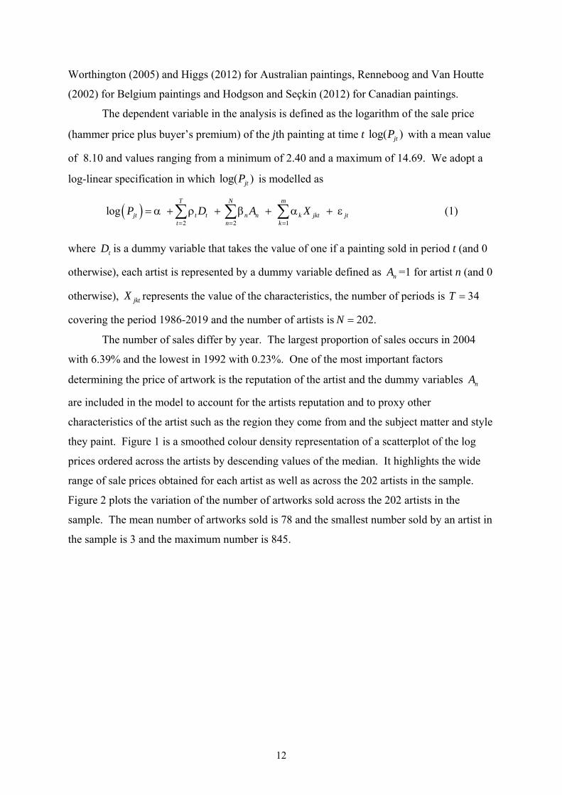
The dependent variable in the analysis is defined as the logarithm of the sale price

(hammer price plus buyer’s premium) of the jth painting at time t log( )jtP with a mean value

of 8.10 and values ranging from a minimum of 2.40 and a maximum of 14.69. We adopt a

log-linear specification in which log( )jtP is modelled as

2 2 1

log T N m

jt t t n n k jkt jtt n k

P D A X

(1)

where tD is a dummy variable that takes the value of one if a painting sold in period t (and 0

otherwise), each artist is represented by a dummy variable defined as nA =1 for artist n (and 0

otherwise), jktX represents the value of the characteristics, the number of periods is 34T

covering the period 1986-2019 and the number of artists is 202.N

The number of sales differ by year. The largest proportion of sales occurs in 2004

with 6.39% and the lowest in 1992 with 0.23%. One of the most important factors

determining the price of artwork is the reputation of the artist and the dummy variables nA

are included in the model to account for the artists reputation and to proxy other

characteristics of the artist such as the region they come from and the subject matter and style

they paint. Figure 1 is a smoothed colour density representation of a scatterplot of the log

prices ordered across the artists by descending values of the median. It highlights the wide

range of sale prices obtained for each artist as well as across the 202 artists in the sample.

Figure 2 plots the variation of the number of artworks sold across the 202 artists in the

sample. The mean number of artworks sold is 78 and the smallest number sold by an artist in

the sample is 3 and the maximum number is 845.

13

Figure 1: Scatterplot of the Logarithm of sale prices at auction by artists ordered by the median price

0 50 100 150 200

2.5

5.0

7.5

10.0

12.5

15.0

The median log price

20

40

60

80

100

Fre

quen

cy

The

log

pric

e

Rank

Figure 2: The distribution of the number of artworks sold at auction by artist.19

Artists Ordered by Median Price 5

10

20

50

100

250

500

1000

Nu

mb

er o

f A

rtw

ork

s S

old

The other characteristics include the size of the painting as represented by the surface

area in square meters (sqa) with mean 1.083 m2 and the surface area squared (sqa2). As the

death of an artist caps the stock of paintings a dummy variable (YD) is included to indicate

whether the artist is deceased at the time of the auction. On average the proportion of artists

19 Only one artist that has sold fewer than 5 pieces is not shown.

14

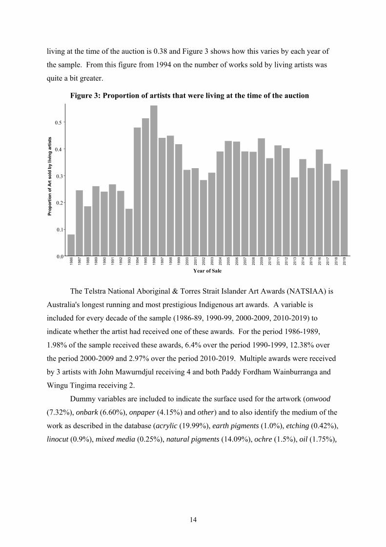
living at the time of the auction is 0.38 and Figure 3 shows how this varies by each year of

the sample. From this figure from 1994 on the number of works sold by living artists was

quite a bit greater.

Figure 3: Proportion of artists that were living at the time of the auction

19

86

19

87

19

88

19

89

19

90

19

91

19

92

19

93

19

94

19

95

19

96

19

97

19

98

19

99

20

00

20

01

20

02

20

03

20

04

20

05

20

06

20

07

20

08

20

09

20

10

20

11

20

12

20

13

20

14

20

15

20

16

20

17

20

18

20

19

Year of Sale

0.0

0.1

0.2

0.3

0.4

0.5

Pro

po

rtio

n o

f A

rt s

old

by

livi

ng

art

ists

The Telstra National Aboriginal & Torres Strait Islander Art Awards (NATSIAA) is

Australia's longest running and most prestigious Indigenous art awards. A variable is

included for every decade of the sample (1986-89, 1990-99, 2000-2009, 2010-2019) to

indicate whether the artist had received one of these awards. For the period 1986-1989,

1.98% of the sample received these awards, 6.4% over the period 1990-1999, 12.38% over

the period 2000-2009 and 2.97% over the period 2010-2019. Multiple awards were received

by 3 artists with John Mawurndjul receiving 4 and both Paddy Fordham Wainburranga and

Wingu Tingima receiving 2.

Dummy variables are included to indicate the surface used for the artwork (onwood

(7.32%), onbark (6.60%), onpaper (4.15%) and other) and to also identify the medium of the

work as described in the database (acrylic (19.99%), earth pigments (1.0%), etching (0.42%),

linocut (0.9%), mixed media (0.25%), natural pigments (14.09%), ochre (1.5%), oil (1.75%),

15

pen (0.13%), pencil (0.14%), polymer paint (0.10%), gouache (0.45%), screenprint (1.40%),

synthetic polymer paint20 (33.27%), watercolour (23.42%) and other.

Dummy variables are also included to account for the 44 auction houses where the

sales take place. Figure 4 shows the distribution of total sales across the sample by the 27

auction houses with over $150,000 in turnover. The market is dominated by Sotheby's21,

Menzies and Deutscher and Hackett.22 For this sample, the highest proportion of sales

occurred in October and the lowest in May. To account for seasonal fluctuations in sales,

monthly dummy variables are included. Overseas sales account for 2.2% of the sales. A

dummy variable is included to indicate whether the painting was sold at an auction that was

held overseas (overseas). Although each painting is treated as a single sale, we also include a

dummy variable to indicate whether the sale was a repeat sale (repeat). In the sample only

2.6% of the sales were identified as being repeat sales23.

Figure 4: Distribution of Auction Turnover by House24

$0 $20 mill $40 mill $60 mill $80 mill

Turnover

Deutscher

Cornette de Saint Cyr

McKenzies Auctioneers

Cromwell's Sydney

ArtCurial

Goodmans Auctioneers

Gaia Auction Paris

Philips Auctions Australia

Davidson Auctions

Phillips De Pury & Company

Theodore Bruce Auctions

GFL Fine Art

Lawsons

Bonhams & Goodman

Joel Fine art

Other

Elder Fine Art

Shapiro Auctioneers

CooeeArt MarketPlace

Leonard Joel

Christies

Deutscher-Menzies

Mossgreen

Bonhams

Lawson-Menzies

Deutscher and Hackett

Menzies

Sothebys

Auction House

20 Note that acrylic and synthetic polymer paints are identical. However, contemporary artists are labelling their paintings synthetic polymer paint rather than using the acrylic label due to a perceived difference in nomenclature see e.g. artistmarketingresources.com. 21 For example as noted by Cascone S. (2015). 22 Note that in some cases the name of the auction house was not consistent, and we report the name as recorded. 23 Due to the lack of an indication that the work had been previously sold we determined if it was a repeat sale if the work had the same: title, artist, description of medium and dimensions, where the sales were at least 120 days apart. 24 The values are in nominal Australian dollars. The other category is the total for auction houses that have less than 150,000 in total turnover.

16

5: Estimation Results and the Art Index

5:1 Estimating the Average Art Index using the OLS Model

The estimated OLS coefficients of the hedonic pricing regression model specified in

(1) are presented in Table 1. To account for an unknown form of heteroskedasticity the

standard errors and corresponding p-values are based on heteroskedastic-consistent standard

errors. The adjusted R2 is 0.732 and the four joint F-tests on the coefficients on the dummy

variables for years, the dummy variables for month, the auction house dummy variables and

the artists fixed effects are all rejected.

Table 1: OLS Estimation Results

Variable OLS Variable OLS Constant 7.263*** Synthetic 1.344*** YD 0.063** Water 0.656*** sqa 0.049* Overseas 0.582*** sqa2 -4.6E-5** Tel80 -2.14*** Onwood 0.559*** Tel90 0.053 Onbark -0.223*** Tel00 0.17** Onpaper -0.285*** Tel10 0.048 Acrylic 0.801*** Repeat 0.042 Earth 1.308*** Fixed Effects Etching -0.749*** Years Yes Linocut -1.094*** Months Yes Mixed 0.904*** Auction houses Yes Natural 1.29*** Artists Yes Ochre 1.239*** Oil 0.691*** Observations 15,845 Pen -0.302

2R 0.732

Pencil 0.121 F tests (years) 46.98*** Polymer 1.049*** F tests (months) 12.02*** Gouache 0.256* F tests (auction houses) 53.26*** Screenprint -0.955*** F tests (artists) 72.35*** Notes: Dependent variable: logarithm of the sale price. The omitted year is 1986, omitted month is April, omitted artist is Rover Thomas, omitted auction house is Ainger, omitted medium is other and omitted surface is other. Significance levels: *** p<0.01, ** p<0.05, * p<0.1 based on heteroskedastic-consistent standard errors.

From Table 1 it can be noted that if the artist is no longer living at the time of sale

(YD) generates a positive effect on the price of the artwork as does sales in overseas auctions.

While the surface area (sqa) has a positive effect on the price of the artwork, the squared term

(sqa2) has a negative effect. This implies that there is an increase in the sales price associated

with an increase in the artwork size but this impact diminishes with increasing size. A

similar result was also found in Higgs and Worthington, (2005). In comparison to other

mediums, acrylic, earth, mixed, natural, ochre, oil, polymer, gouache and synthetic are more

expensive whereas etching, linocut, pen and screenprint are less expensive. Artworks on

17

wood (onwood) are more expensive compared to artworks on other surfaces whereas those on

bark (onbark) and on paper (onpaper) are less expensive. The results also suggest that

artworks are more expensive for those who received Telstra National Aboriginal & Torres

Strait Islander Art Awards in the 2000’s but less expensive in the 1980’s.

The estimates of t can be used to form an art price index conditioned on the other

explanatory variables included in (1). The level of the art price index is defined as 100 for

the year 1986. For subsequent years, the price index is computed by exponentiating the

estimates of t . That is, the estimated price index for 1987 is 2ˆ100exp , at time 1988 is

3ˆ100exp and up to 2019 which is 34

ˆ100exp . A plot of the nominal art price index is

shown in Figure 5. To provide a comparison with Australian financial assets also plotted in

Figure 5 is the nominal All Ordinaires price index. As both art and housing can be

considered as consumption and investment goods (Higgs 2012), the housing price index is

also plotted. The All Ordinaires price index tracks the movements of the 500 largest

companies listed on the Australian Securities Exchange (ASX) accounting for over 95% of

all the shares listed on the ASX and is used here to provide a comparison between the art

market and Australian financial assets. The Australian housing price index is the weighted

prices for eight Australian capital cities produced by the Australian Bureau of Statistics.25

Highlighted in Figure 5 are the periods of the GFC, the introduction of the RRS, the

period of the self-managed superfund changes (SUPER) and the 2018 amendment to the

Protection of the Moveable Cultural Heritage Act 1986 (PMCH). Over the sample period, we

see that the housing price index has been steadily increasing with moderate falls in 2010 and

more recently in 2019. The All Ordinaries stock index and Art Price indices had similar

profiles up until the GFC and they also both fell during the period of the GFC. However, the

All Ordinaries stock index increased again from 2010 followed by a moderate fall in 2011

but by 2019 it was slightly higher than its 2007 value. The Art Price index though, continued

to fall until a slight increase in 2013 although in 2014 there was another fall followed by only

moderate increases and by 2019 it had still not reached its 2007 value.

25 ABS 6416.0 - Residential Property Price Indexes: Eight Capital Cities

18

Figure 5: Art Price, All Ordinaires and Housing Price Indices

Figure 6 shows a comparison of the annual returns for the three markets.26 There was

a world art market downturn in the 1990s (Higgs 2012) and in Figure 6 a large fall in returns

in the art market occurred in 1995. During the period of the GFC we see falls in both art and

All Ordinaires returns. For art returns we also see falls in 2010 and 2014 and we do not see

corresponding falls in these time periods for either the All Ordinaries or housing.

Figure 6: Art Price, All Ordinaires and Housing Price Returns

26 Annual returns are calculated as 1ˆ ˆ100 exp 1t t

020

040

060

080

0

-40

-20

020

40

198

71

988

198

91

990

199

11

992

199

31

994

199

51

996

199

71

998

199

92

000

200

12

002

200

32

004

200

52

006

200

72

008

200

92

010

2011

201

22

013

201

42

015

201

62

017

201

82

019

19

5:2 The Quantile Art Index

Prices of artworks sold in the sample vary widely from a minimum value of $11 to a

maximum value of $2,400,000. This suggests a possible segmentation in the art market with

respect to price. In order to analyze the segments of the market separately we can model the

different price quantiles as different segments of the market. This can be done by use of

quantile regression (Koenker and Bassett 1978). In the regressions estimated in Section 4 we

assumed that we were modelling the conditional mean of the prices. By contrast the quantile

regression approach models the conditional quantiles of the prices.

The quantiles of a random variable are parameters of the distribution just as the

expected value and the variance are. They are defined as the percentage levels of the

variable. The most commonly referred to quantile is the 50% of the variable. Just as the

average of the variable can be used to estimate the expected value (µ) of the variable as:

( )xf x dx

(2)

where for the random variable x with a probability density defined by ( )f x . The 50%

quantile of the same random variable is defined as the value of x where the probability

of all values below it is equal to .50 or 50( ) .50P x that is defined as:

50

.50 ( )f x dx

. (3)

Thus 50 can be estimated can be estimated via the mid-point (or median) of the

observations.27 Other quantiles can be defined by different percentages. Thus, for any

quantile q (where 0 1q ) which is defined as ( )qP x q and formally we have:

( )q

q f x dx

(4)

The estimates of q can be found from the empirical cumulative density of the data by

finding the value that corresponds to the qth value of the data. Alternatively, if we sort the

observations in ascending order the quantiles can be found by the values of x at each

percentage.

27 Nomenclature is difficult here since many text book treatments refer to the mid-point value as the median where the 50% percentile is a parameter of the distribution and not the estimate.

50( )

20

Figure 7 is a plot of the empirical cumulative distribution function of the log

transformation of the prices ( log( )jtP that is used as the dependent variable in (1)) except that

the axes are reversed. From this plot we can locate the values of the log( )jtP that define the

various quantiles. From Figure 7 we can read the qth quantile of the log prices where

0 1q , 10ˆ 5.8 , 25

ˆ 6.7 , 50ˆ 8.1 , 75

ˆ 9.2 and 90ˆ 10.2 . Which are equivalent to

$330, $812, $3,294, and $26,903 respectively.

Figure 7: Quantiles of the Dependent Variable

0

5

10

15

0 .2 .4 .6 .8 1Proportion of the data

qth Q

uant

ile

of t

he l

og p

rice

s

10ˆ 5.8

25ˆ 6.7

50ˆ 8.1

75ˆ 9.2

90ˆ 10.2

Renneboog and Spaenjers (2013) provide three reasons for the segmentation of the art

market. First, art is indivisible so typically small investors are not able to invest in high-end

work. Secondly, wealthy individuals may be less likely to buy in the lower end of the market

as these works may not necessarily signal the same social status. Thirdly, the more expensive

parts of the market may be prone to speculation.

In this section we use quantile regression to examine art characteristics and to develop

indices across the price distribution. Quantile regression estimates the conditional qth

quantile of the dependent variable for 0 1q . For example, q= 0.5 (or median) measures

the middle value price of artworks given certain characteristics, whereas the 0.1 quantile

represents a lower segment and the 0.9 quantile an upper segment. The conditional quantile

model for the dependent variable iy given the independent variables ix is given by,

i

qy i iQ q x x (5)

21

where, logi jty P and 2 2 1

.T N m

qi t t n n k jkt

t n k

x D A X

The coefficients of the qth

quantile of the conditional distribution are defined as a solution to the minimization problem

(Koenker and Bassett 1978)

: :

min 1i i i i

q qi i i i

i y x i y x

q y x q y x

(6)

Although the optimization defined by (6) does not have an explicit solution we can

find a solution when (6) is posed as a linear programming problem. The estimation results

and pseudo-R2 for five different quantiles, q=0.1, 0.25, 0.5, 0.75 and 0.9 are shown in Table

2.28 Standard errors for the quantile regression are obtained using the XY-pair bootstrap

method with 100 replications. Also shown in this Table are the F-tests for the joint

significance on the coefficients of the year dummy variables, the dummy variables for month,

the auction house dummy variables and the artists fixed effects. The F-tests are all

significant for all quantiles. Table 3 reports Wald-tests on the equality of slope parameters

(that the parameters estimated for the different quantiles are equal) for two quantile

comparisons (0.1, 0.5) and (0.5, 0.9).

The quantile regression results indicate that artwork at varying price levels is

influenced in different ways by their characteristics. Although the quadratic term on the

surface area (sqa2) is not significant for any of the quantiles, the linear term is significant for

each quantile and increasing with higher quantiles. The slope equality test on the linear term

(sqa) can be rejected for both quantile pairs (0.1, 0.5) and (0.5, 0.9) this implies that the size

of the artwork influences the price to a greater and greater extent for art in the different price

segments.

In the case of the different mediums we get differences between price segments for

wood but not bark or paper. The estimated coefficients for the onwood characteristic are

positive and significant and increase in magnitude across all the quantiles although a slope

equality test can only be rejected for the (0.1, 0.5) pair. However, for both onbark and

onpaper, a slope equality test cannot be rejected at either of the quantile pairs (0.1, 0.5) and

(0.5, 0.9).

In the case of the mediums, the estimated coefficients for acrylic, earth, mixed,

natural, ochre, oil, polymer and synthetic are positive and significant for all quantiles

although the estimated coefficients consistently decrease in magnitude with higher quantiles.

28 The pseudo-R2 is calculated according to Koenker and Machado (1999).

22

Further, the slope equality test can be rejected for both quantile pairs (0.1, 0.5) and (0.5, 0.9)

except for mixed where neither can be rejected.

The pattern for the estimated coefficients on gouache, pencil and water follow a

similar pattern to the other mediums. However, the estimated coefficients are only

significant for the lower quantiles. The slope equality test is rejected for both quantile pairs

(0.1, 0.5) and (0.5, 0.9) for gouache but only for the (0.1, 0.5) pair for pencil and water.

The estimated coefficients for etching and linocut are negative and decreasing in

value with higher quantiles. Further, they are only significant for the higher quantiles

although for etching the slope equality test can be rejected for both quantile pairs (0.1, 0.5)

and (0.5, 0.9) whereas it can only be rejected for the (0.5, 0.9) pair for linocut.

For screenprint the estimated coefficients are also negative and decreasing in value

with higher quantiles and are significant for all quantiles except the 0.1 quantile. A slope

equality test is rejected for both quantile pairs (0.1, 0.5) and (0.5, 0.9). The slope equality

tests cannot be rejected at either of the quantile pairs (0.1, 0.5) and (0.5, 0.9) for repeat, yd,

overseas and for all of the awards variables (Tel80, Tel90, Tel00 and Tel10).

We observe some heterogeneity across the quantiles for auction houses, particularly

among the higher quantiles. Individual slope equality tests can be rejected for 95% of the

coefficients on auction houses between the 0.5 and 0.9 quantiles whereas only 10% can be

rejected between the 0.1 and 0.5 quantiles.29 Figure 1 highlights the heterogeneity in the

prices each artist received for their artwork. This can also be seen in the results of the

individual slope equality tests on the coefficients for the artists fixed effects as 60% can be

rejected between the (0.5, 0.9) quantiles and 40% between the (0.1, 0.5) quantiles. However,

no individual slope equality tests can be rejected for any of the coefficients on the month

dummy variables between either the (0.1, 0.5) quantiles and the (0.5, 0.9) quantiles.

29 For auction houses, artist, months and years the percentages of the slope equality tests that could be rejected were based on 1, 5 and 10% levels of significance.

23

Table 2: Quantile Regression Results

Variable Q0.1 Q0.25 Q0.5 Q0.75 Q0.9 Variable Q0.1 Q0.25 Q0.5 Q0.75 Q0.9 C 5.43*** 5.978*** 6.493*** 7.485*** 9.329*** Synthetic 1.825*** 1.486*** 1.24*** 0.808*** 0.637*** YD 0.042 0.071** 0.091*** 0.068** 0.055 Water 1.677*** 1.078*** 0.586*** 0.194 0.285 sqa 0.034** 0.045*** 0.053*** 0.060*** 0.063*** Overseas 0.225 0.144 0.41** 0.602*** 0.607*** sqa2 -0.000 -0.000 -0.000 -0.000 -0.000 Tel80 -2.51*** -2.33*** -2.21*** -2.21*** -2.33*** Onwood 0.350*** 0.485*** 0.838*** 0.986*** 0.912*** Tel90 0.028 0.117 -0.07 0.092 0.272* Onbark -0.067 0.049 0.143* 0.258*** 0.219 Tel00 0.099 0.094 0.287*** 0.272*** 0.31*** Onpaper -0.170*** -0.205*** -0.143*** -0.151*** -0.108** Tel10 0.229 0.161*** 0.08* 0.098* 0.018 Acrylic 1.326*** 0.961*** 0.796*** 0.392*** 0.289*** Repeat -0.048 0.004 0.003 -0.05 0.006 Earth 1.718*** 1.335*** 1.311*** 0.846*** 0.758*** Fixed Effects Etching 0.164 -0.252 -0.424*** -0.724*** -0.987*** Years Yes Yes Yes Yes Yes Linocut 0.21 -0.469 -0.593* -0.935*** -1.388*** Months Yes Yes Yes Yes Yes Mixed 1.019*** 0.921** 0.901*** 0.649*** 0.701*** Auction houses Yes Yes Yes Yes Yes Natural 1.664*** 1.369*** 1.280*** 0.820*** 0.635*** Artists Yes Yes Yes Yes Yes Ochre 1.596*** 1.187*** 1.178*** 0.79*** 0.919*** Oil 1.217*** 0.921*** 0.807*** 0.518*** 0.359*** Observations 15,845 15,845 15,845 15,845 15,845

Pen 0.499 -0.75 -0.675 -1.454* 0.066 Pseudo2

R 0.491 0.544 0.561 0.562 0.556

Pencil 0.929** 0.599* 0.056 0.092 -0.15 F tests (years) 38.97*** 56.19*** 45.22*** 30.49*** 23.68*** Polymer 1.792*** 1.206*** 0.998*** 0.502*** 0.222 F tests (months) 2.75*** 7.04*** 5.71*** 4.67*** 3.69*** Gouache 1.278*** 0.873*** 0.581*** 0.1 0.022 F tests (auction houses) 19.93*** 41.24*** 62.19*** 35.80*** 34.71*** Screenprint -0.212 -0.578*** -0.72*** -1.092*** -1.297*** F tests (artists) 32.69*** 62.55*** 70.38*** 96.67*** 34.48***

Notes: Dependent variable: logarithm of the sale price. The 2

R is Pseudo 2

R calculated according to Koenker and Machado (1999). Significance levels: *** p<0.01, ** p<0.05, * p<0.1 based on standard errors obtained using the XY-pair bootstrap method with 100 replications.

24

Table 3: Slope Equality Tests for two quantile pairs (0.1, 0.5) and (0.5, 0.9).

Variable (0.1,0.5) (0.5,0.9) Variable (0.1,0.5) (0.5,0.9) YD 0.307 0.416 Gouache 0.008 0.009 sqa* 0.034 0.000 Screenprint 0.006 0 Onwood 0.000 0.520 Synthetic 0 0 Onbark 0.144 0.574 Water 0 0.269 Onpaper 0.624 0.512 Overseas 0.424 0.253 Acrylic 0.001 0.000 Tel80 0.239 0.637 Earth 0.045 0.002 Tel90 0.839 0.100 Etching 0.019 0.001 Tel00 0.116 0.829 Linocut 0.298 0.025 Tel10 0.409 0.488 Mixed 0.785 0.555 Repeat 0.446 0.964 Natural 0.017 0.000 Years* 0 0 Ochre 0.022 0.085 Months* 0.817 0.165 Oil 0.035 0.002 Auction houses* 0 0 Pen 0.721 0.390 Artists* 0 0 Pencil 0.062 0.675 Notes: These are the Koenker and Bassett (1982) test for the equality of the slope coefficients across quantiles. p-values reported. * These are the joint tests reported.30

The estimated coefficients on the year dummy variables consistently fall between the

0.1 and 0.5 quantiles whereas there is no consistent pattern between the higher-level

quantiles. Further, at the lower quantiles 91% of the individual slope equality tests on each of

the year dummy coefficients between the (0.1, 0.5) quantiles can be rejected but none can be

rejected between the (0.5, 0.9) quantiles.

Figure 8 provides plots of the estimated coefficients and their confidence intervals for

the different mediums based on a comparison of the OLS and LAV (50% quantile). These

comparisons are less formal than the tests reported in Table 3 however they provide a visual

representation of these types of comparisons. From this plot we note there are no coefficients

were both are significant but that differ in their sign. Except for the Gouache medium in all

other cases the estimated coefficients for each medium have equivalent coefficients. Because

the LAV estimates are more robust to outliers for the dependent variable they tend to be of

smaller magnitude than the OLS values.

30 The individual values of these parameter estimates are plotted in the appendix.

25

Figure 8 Coefficient plot of the Medium Characteristics for the LAV and OLS Estimates.

WATER

SYNTHETIC

SCREENPRINT

POLYMER

PENCIL

PEN

ONWOOD

ONPAPER

ONBARK

OIL

OCHRE

NATURAL

MIXED

LINOCUT

GOUACHE

ETCHING

EARTH

ACRYLIC

-2 -1 0 1

OLSLAVEstimation Method

Figure 9 is the equivalent to Figure 8 except where the comparison of coefficient

estimates is between the 10% and 90% quantiles. In this case we note that the contributions

of most of the medium characteristics generally have a greater influence on the sale price in

the model of the lower 10% versus in the 90% model. However, there are exceptions for the

estimated coefficients for those on wood and on paper. This would indicate that works on

these mediums tend to be less valuable in the lower tier of the market than the upper tier.

Figure 9 Coefficient Plot of the Medium Characteristics for the 10% and 90% Quantile Estimates.

WATER

SYNTHETIC

SCREENPRINT

POLYMER

PENCIL

PEN

ONWOOD

ONPAPER

ONBARK

OIL

OCHRE

NATURAL

MIXED

LINOCUT

GOUACHE

ETCHING

EARTH

ACRYLIC

-2 0 2

90%10%Estimation Method

26

Figure 10 plots the nominal art price index constructed for each of the quantile

regressions as well as for OLS. While there is little difference in the profiles of the indices at

the higher-level quantiles there is at the lower quantile levels. For the lower-level quantiles

the index is higher for every year than the corresponding index at the higher-level quantiles

and OLS. Also, in 2011 the lower-level quantile indices seem to be slightly increasing

whereas the OLS and higher-level indices are still falling. This finding appears to confirm

the negative "masterpiece effect" that has been observed by several researchers in prices paid

for contemporary and impressionist work.31

Figure 10: Art Price Indices based on OLS and Quantile Estimates

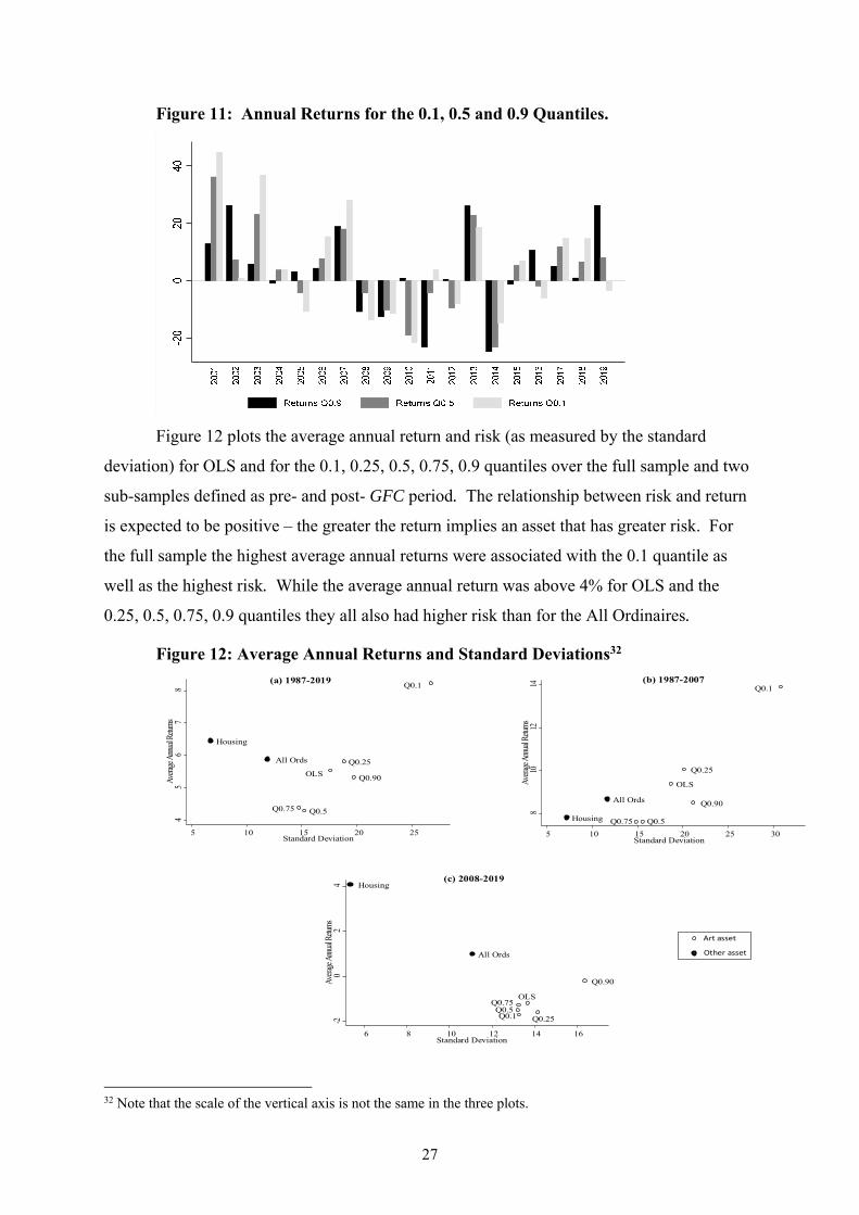
Figure 11 shows a comparison of the annual returns for the 0.1, 0.5 and 0.9 quantiles.

During the period of the GFC we see falls in annual returns for all the quantiles. Around the

time of the introduction of the Resale Royalty Scheme in 2010 we see falls in the annual

returns for the 0.1 and 0.5 quantiles. Corresponding to the introduction of changes to self-

managed super funds we see a large fall in the annual returns for the 0.9 quantile and a

smaller fall for the 0.5 quantile in 2011 and falls in all the annual returns for the 0.1, 0.5 and

0.9 quantiles in 2014.

31 The masterpiece effect proposes that prices of high value works will appreciate faster than lower value works. See the comparison of the results of previous attempts to find this effect in Table 2 in Ashenfelter and Graddy (2003).

27

Figure 11: Annual Returns for the 0.1, 0.5 and 0.9 Quantiles.

Figure 12 plots the average annual return and risk (as measured by the standard

deviation) for OLS and for the 0.1, 0.25, 0.5, 0.75, 0.9 quantiles over the full sample and two

sub-samples defined as pre- and post- GFC period. The relationship between risk and return

is expected to be positive – the greater the return implies an asset that has greater risk. For

the full sample the highest average annual returns were associated with the 0.1 quantile as

well as the highest risk. While the average annual return was above 4% for OLS and the

0.25, 0.5, 0.75, 0.9 quantiles they all also had higher risk than for the All Ordinaires.

Figure 12: Average Annual Returns and Standard Deviations32

Q0.1

Q0.25

Q0.5Q0.75

Q0.90OLS

All Ords

Housing

45

67

8Av

erage

Annu

al Re

turns

5 10 15 20 25Standard Deviation

(a) 1987-2019Q0.1

Q0.25

Q0.5Q0.75

Q0.90

OLS

All Ords

Housing

810

1214

Avera

ge An

nual

Retur

ns

5 10 15 20 25 30Standard Deviation

(b) 1987-2007

Q0.1 Q0.25Q0.5

Q0.75

Q0.90

OLS

All Ords

Housing

-20

24

Avera

ge An

nual

Retur

ns

6 8 10 12 14 16Standard Deviation

(c) 2008-2019

Art asset

Other asset

32 Note that the scale of the vertical axis is not the same in the three plots.

28

However, a different pattern emerges when the pre- and post-GFC subsamples are

considered. For the pre-GFC subsample each have a similar or higher average annual return

than housing as well as a higher risk which matches the idea of higher risk resulting in higher

returns for works from all segments of the market. However, for the post-GFC subperiod

while all segments of the art market have higher risk than either housing or the All Ordinaries

stock index, they also have a negative average annual return. This suggests that the GFC and

Government policies since 2008 have had a strong impact on the art market.

In comparison to the global art market we find that while both sales and volumes fell

sharply in 2009, there was a strong rebound for the period 2009-2011 following the GFC

(Solimano 2019). Etro and Stepanov (2019) develop a global art price index for

contemporary artists based on Western art and more than 500 artists using repeated sales.

They show that for contemporary art prior to 2007 there was a rapid increase in prices and

although there was a substantial decline during the GFC there has subsequently been a

sustained increase. Their art price index is illustrated in Figure 13 (solid line) and for

comparison the AAA price index is shown based on OLS estimates (dashed line) where both

are scaled to start at 100 in 2000. This highlights a prolonged decrease in price changes for

aboriginal art with only a recent slight increase.

Figure 13: Comparison of the estimated mean price index and the global price index for top contemporary western artists.

50

100

150

200

250

300

350

400

450

2000 2002 2004 2006 2008 2010 2012 2014 2016 2018

Price index for contemporary artists based on Western art

Aboriginal art price index

6: Discussion

In this paper we have estimated the price index for the Australian Aboriginal Art

market by collecting the sale price and the characteristics of 15,845 works of art that were

sold at auction from 1986 to 2019 by 202 artists. The characteristics of these works were

29

determined from the auction catalogues. These include the time sold, the medium of the

work, the dimensions of the work, the auction house were sold and the status of the artist.

This model allows us to determine how the market for these works changed over time in

order to estimate a price index for this period. The variation in value of these artworks over

this period is particularly important due to the changes in Australian Federal legislation

concerning the status of these artwork as investment assets and the requirement to adhere to

the Resale Royalty Act.

We find that the value of these artwork fell after these changes to the investment

status of these works and the rates of return for these works as investment assets fell to the

point where they became negative for a longer period than art work in other countries after

the Global Financial Crisis. Using a quantile regression approach, we were able to subdivide

the impacts of these changes by the segment of the market. In doing so we identified

significant differences between the impacts of these changes for artwork in the top 10% of

the market from the rest of the market. This approach allowed us to estimate separate price

indices for these different aspects of the market.

A caveat to our findings is the inherent limitations in the price data we employ for our

analysis. In the 2019 global art market sales of 64.1 billion $US only 24.2 billion $US or less

than 38% were estimated to be sold at auction (page 19 McAndrew 2020) with the remainder

sold by dealers, at art fairs and on-line. In addition, we have no indication of the number of

works that came to auction but did not sell nor do we know the actual transaction for the item

since there are usually significant auction costs. Also, when comparing the rates of return of

investments, we have not included the significant frictional costs in the market. The 10 to

17.5% buyer's premium charged the buyer and the 10% sellers commission would indicate

that the price of an artwork would need to rise by up to 27.5% for a seller to make a profit

from the sale.

Recently there is a growing concern that the rapid increase in the value of art sales has

been fueled by money laundering activities which has resulted in the imposition of a more

regulated art market (page 80 McAndrew 2020). This new set of requirements on the

provenance of art and the details of ownership has increased costs for the sellers of art but on

the other hand may lead to a more stable market for art.33

33 Due to the remote locations of some Aboriginal artists, the provenance a few works has been an issue as documented in Chappell and Hufnagel (2014).

30

References

Acker, T. (2016), “Somewhere in the world: Aboriginal and Torres Strait Islander art and its place in the global art market”, CRC-REP Research Report CR017. Ninti One Limited, Alice Springs.

Ashenfelter, O., K. and Graddy, (2003) "Auctions and the Price of Art", Journal of Economic Literature, 41, 763-786.

Cascone S. (2015), “$2 Million Aboriginal Art Auction Pays Off for Sotheby’s London”, artnet, June 11.

Challis D. (2019), “The Australian art market has flatlined. What can be done to revive it?”, The Conversation, Sept. 27.

Chappell D., S. and Hufnagel (2014), ‘Case Studies on Art Fraud: European and Antipodean Perspectives’ in Contemporary Perspectives on the Detection, Investigation and Prosecution of Art Crime, Eds. Chappell D and Hufnagel S, Ashgate Publishing Ltd., England, pp. 57 – 77.

Chwelos P. (2003), “Approaches to Performance Measurement in Hedonic Analysis: Price Indexes for Laptop Computers in the 1990s”, Economics of Innovation and New Technology, 12, 199–224.

Court A. (1939), “Hedonic Price Indexes with Automotive Examples.” In: The Dynamics of Automobile Demand, edited by V. von Szeliski, S. Horner, and C. Roos, 99–117. New York: The General Motors Corporation.

Deloitte, ArtTactic, (2019), Art & Finance Report 2019, https://www2.deloitte.com/content/dam/Deloitte/global/Documents/Finance/gx-fsi-art-and-finance-report-2019.pdf

Demir E., Gozgor G. and Sari E. (2018), “Dynamics of the Turkish paintings market: A comprehensive empirical study”, Emerging Markets Review, 36, 180-194.

Etro, F. and E. Stepanova (2019), "On the Efficiency of Art Markets. Evidence of return rates from old masters' paintings to contemporary art." University of Florence, Working Paper 29, September. https://www.disei.unifi.it/upload/sub/pubblicazioni/repec/pdf/wp29_2019.pdf

Fernandez-Cornejo, J. and S. Jans (1995), “Quality-adjusted Price and Quantity Indices for Pesticides.” American Journal of Agricultural Economics, 77, 645–659.

Genocchio, B. (2008), Dollar Dreaming inside the Aboriginal Art World, Hardie Grant Books, Melbourne.

Griliches Z. (1961), “Hedonic Price Indexes for Automobiles: An Econometric Analysis of Quality Change.” in The Price Statistics of the Federal Government, General Series No. 73, edited by Price Statistics Review Committee, 137–196. New York: Columbia University Press.

Higgs H. and Worthington A. (2005), “Financial Returns and Price Determinants in the Australian Art Market, 1973–2003”, Economic Record, 81, 113–123.

Higgs H. (2012), “Australian Art Market Prices during the Global Financial Crisis and Two Earlier Decades”, Australian Economic Papers, 51, 189–209.

31

Hodgson D. and Seçkin A. (2012), “Dynamic Price Dependence of Canadian and International Art Markets: An Empirical Analysis”, Empirical Economics, 43, 867–890.

Koenker R. and Bassett, G. (1978), “Regression Quantiles”, Econometrica, 46(1), 33-50.

Koenker R. and Bassett, G. (1982). “Robust Tests for Heteroskedasticity Based on Regression Quantiles,” Econometrica, 50, 43-62.

Koenker R. and Machado J. (1999), “Goodness of Fit and Related Inference Processes for Quantile Regression”, Journal of the American Statistical Association, 94, 1296–1310.

Lamont L. (2011), “Art investors painted into tight corner”, The Sydney Morning Herald, 14 March

Lehman-Schultz C. (2013), “How super laws are killing the market for Indigenous art”, The Conversation, Nov. 1, 2013.

Lye J. and J. Hirschberg (2017), “Secondary school fee inflation: an analysis of private high schools in Victoria, Australia”, Education Economics, 25, 482-500.

McAndrew, C. (2020), The Art Market 2020, An Art Basel & UBS Report. https://d2u3kfwd92fzu7.cloudfront.net/The_Art_Market_2020-1.pdf.

Renneboog L. and Spaenjers, C. (2013), “Buying Beauty: On Prices and Returns in the Art Market”, Management Science, 59, 36-53.

Renneboog L. and van Houtte T. (2002), “The Monetary Appreciation of Paintings: From Realism to Magritte”, Cambridge Journal of Economics, 26, 331–358.

Rosen S. (1974), “Hedonic Prices and Implicit Markets: Product Differentiation in Pure Competition.” Journal of Political Economy,82, 34–55.

Schwartz A. and B. Scafidi (2004), “What’s Happened to the Price of College? Quality-adjusted Net Price Indexes for Four-year Colleges”, The Journal of Human Resources, 39, 723–745.

Simpson S (2015), Review of the Protection of movable Cultural Heritage Act 1986, downloaded https://www.arts.gov.au/sites/default/files/borders-of-culture-review-of-the-protection-of-movable-cultural heritage-act-1986-final-report-2015.pdf?acsf_files_redirect 5th June 2020.

Solimano A. (2019), “The Art Market at Times of Economic Turbulence and High Inequality”, downloaded https://institute.eib.org/wp-content/uploads/2019/06/Art-Market-Economic-Trubulence-Inequality-Paper-Solimano.pdf, 25th Feb 2020.

Taylor D. and L. Coleman (2011), “Price determinants of Aboriginal art, and its role as an alternative asset class”, Journal of Banking and Finance, 35, 1519–1529.

Wilson-Anastasios M. (2019), “Health check due on Resale Royalty Scheme as data murky on Indigenous beneficiaries”, Oct 3rd, The Sydney Morning Herald.

Witkowska D. (2014), “An Application of Hedonic Regression to Evaluate Prices of Polish Paintings”, International Advances in Economic Research, 20, 281–293.

32

Appendix Estimated Coefficient plots

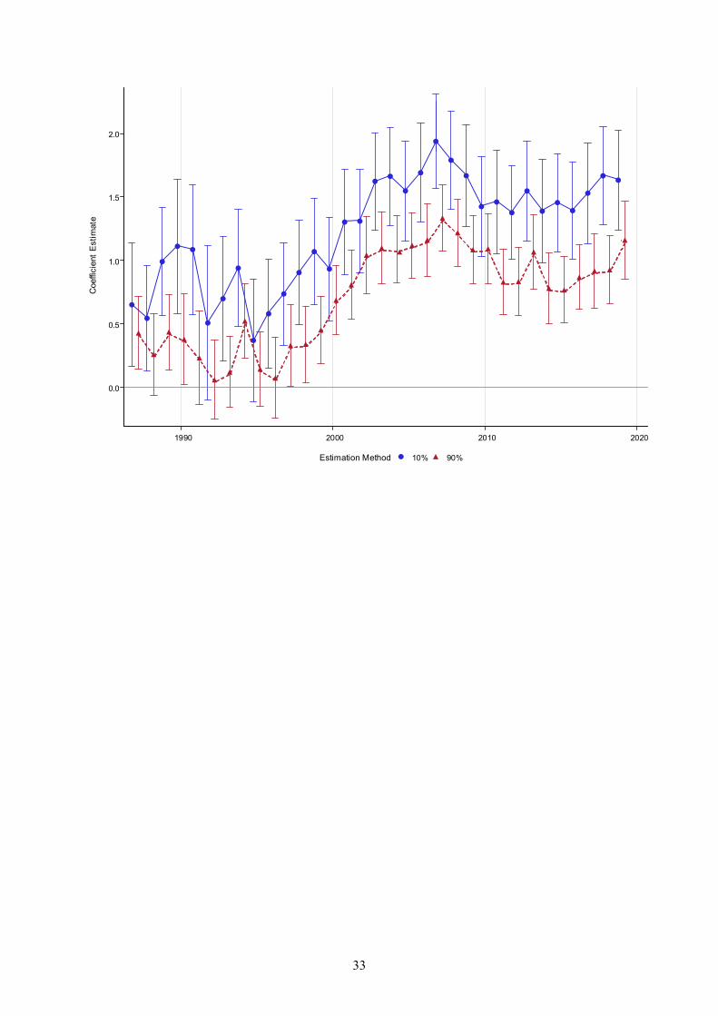
Figure A.1 The year indicator variables

1990 2000 2010 2020

-0.5

0.0

0.5

1.0

1.5

2.0

Coe

ffici

ent

Est

imat

e


33

1990 2000 2010 2020

0.0

0.5

1.0

1.5

2.0

Coe

ffici

ent

Est

imat

e


34

Figure A.2 The Auction House Indicator Variables

Webb's


Stanley and Co

sothebys

Small & Whitfield Auctions

Shapiro Auctioneers

Scammell Auctions

Raffan Kelaher & Thomas P/L



Spink Auctions

Mossgreen

Lawson-Menzies


Mason Gray

Leski Auctions Pty Ltd

Leonard Joel

Lawsons

Joel Fine art

Gregsons


Gibson's Auctioneers & Valuers

Geoff K Gray

Gaia Auction Paris

GFL Fine Art

Elder Fine Art

Dunbar Sloane

Deutscher-Menzies


Davidson Auctions

Cromwell's Sydney

The Collection of Arnaud Serval


Christies

Canberra Antique Auctions

Bonhams

Bay East Auctions

Barsby Auctions

Badgery's Auctioneers

Aust. Art Auctions

ArtCurial

Archers Auctioneers & Valuers

Amanda Addams Auctions

hous

e

-2 -1 0 1

Coefficient Estimate


Auction House Parameter Estimates with 95% Confidence LimitsComparison of OLS and LAV

35

Webb's


Stanley and Co

sothebys

Small & Whitfield Auctions

Shapiro Auctioneers

Scammell Auctions

Raffan Kelaher & Thomas P/L



Spink Auctions

Mossgreen

Lawson-Menzies


Mason Gray

Leski Auctions Pty Ltd

Leonard Joel

Lawsons

Joel Fine art

Gregsons


Gibson's Auctioneers & Valuers

Geoff K Gray

Gaia Auction Paris

GFL Fine Art

Elder Fine Art

Dunbar Sloane

Deutscher-Menzies


Davidson Auctions

Cromwell's Sydney

The Collection of Arnaud Serval


Christies

Canberra Antique Auctions

Bonhams

Bay East Auctions

Barsby Auctions

Badgery's Auctioneers

Aust. Art Auctions

ArtCurial

Archers Auctioneers & Valuers

Amanda Addams Auctions

hous

e

-2 0 2



Auction House Parameter Estimates with 95% Confidence LimitsComparison of 10% and 90%

36

Figure A.3 The Repeat sales, Sold out of Australia, Sold after death and Telstra Awards Indicator Variables

YD

TEL90

TEL80

TEL10

TEL00

REPEAT

OVERSEAS

Var

iabl

e

-2 -1 0 1



Other Parameter Estimates with 95% Confidence LimitsComparison of OLS and LAV

YD

TEL90

TEL80

TEL10

TEL00

REPEAT

OVERSEAS

Var

iabl

e

-3 -2 -1 0 1



Other Parameter Estimates with 95% Confidence Limits

Comparison of 10% and 90%

37

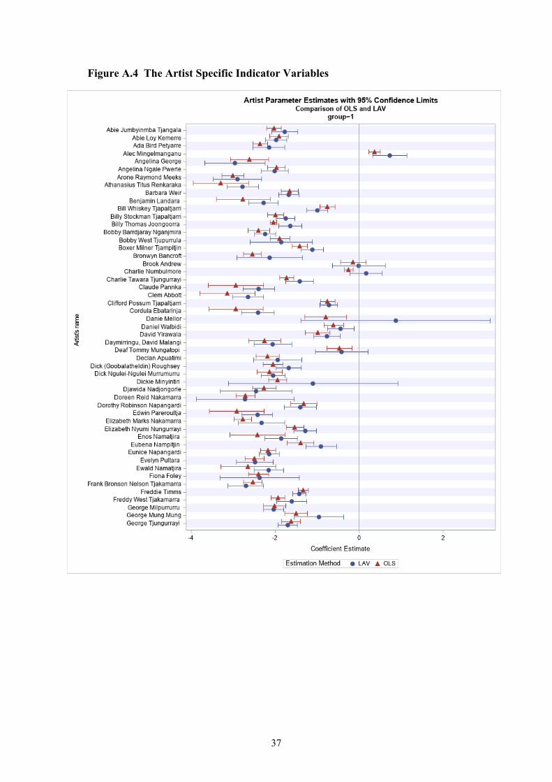
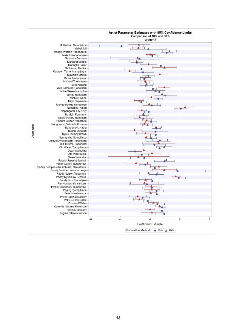
Figure A.4 The Artist Specific Indicator Variables