investment and uncertainty with time to build
TRANSCRIPT
Investment and Uncertainty With Time to Build:
Evidence from U.S. Copper Mining
Margaret E. Slade1
Vancouver School of Economics
The University of British Columbia
Vancouver, BC V6T1Z1
Canada
Email: [email protected]
November 2013
PRELIMINARY DRAFT
Abstract:The standard real–options model predicts that increased uncertainty discourages investment.When projects are large and take time to build, however, this prediction can be reversed.I investigate the investment/uncertainty relationship empirically using historical data onopening dates of new U.S. copper mines — large, irreversible projects with substantial con-struction lags. Both the timing of the decision to go forward and the price thresholds thattrigger that decision are assessed. I find that, in this market, greater uncertainty encouragesinvestment and lowers the price thresholds.
JEL classifications: G11, L72, Q39
Keywords: Investment, Uncertainty, Real options, Copper mining, Exhaustible resources
1 I would like to thank Avner Bar–Ilan, Robert Pindyck, and Joris Pinkse for thoughtful suggestions.

1 Introduction
The standard real options model of investment timing predicts that, since waiting allows
investors to obtain new information about market conditions, increased uncertainty discour-
ages investment.2 In other words, when market conditions are uncertain, investors possess
a valuable call option that is lost when an irreversible decision is made. However, Bar-Ilan
and Strange (1996) show that, when it takes time to build and funds must be committed
up front, flexibility at the completion date also gives investors a put option.3 Since these
two forces work in opposite directions — the first discouraging and the second enouraging
investment — it is impossible to predict theoretically which will prevail. Moreover, there
is little empirical work on large irreversible projects that demonstrates that reversal of the
standard result is a reality and not just a theoretical possibility.4
The ideal setting for assessing the possibility that uncertainty can encourage investment
requires data on projects where i) the investor makes a 0/1 decision to go ahead or to wait,
ii) there are substantial investment lags, iii) once a decision has been made it is di�cult to
alter the scale of the project, iv) there is some flexibility upon completion, and iv) there is
considerable uncertainty. This study uses data on investment in U.S. copper mining — the
opening of new mines — over the 1835 to 1986 period. Copper mines are large irreversible
projects that take time to build. Moreover, the size of the processing facility, the smelter or
leaching plant, fixes the scale of the project several years in advance of completion. When
completion nears, however, it is possible to delay opening, to abandon the mine, or to declare
bankruptcy. Finally, copper prices, like commodity prices in general, are notoriously volatile.
Since I consider a single industry, many factors that would vary across industries can
be ignored. Furthermore, since that industry produces a homogenous product, there is a
well defined output price and variation in that price is the principal source of uncertainty
for investors. Finally, assessing go/no go decisions rather than investment flows leads to a
cleaner test of the real options models. Unfortunately, however, there are also disadvantages
to my approach. Indeed, within an industry, investment in very large–scale projects is apt
to be an infrequent event. When this is true, the data must span a long time period, 150
years in this case, which implies that imperfect proxies for some of the key variables must
be used.
Two aspects of the investment problem are assessed: the timing of the irreversible decision
and the price thresholds that trigger investment. With both the standard model and the
2 See, e.g., Dixit and Pindyck (1994).3 In the context of learning by doing and immediate entry, Roberts and Weitzman (1981) show that
endogenous learning can also reverse the standard results.4 A few studies have found a positive relationship between uncertainty and investment (e.g., Mohn and
Misund (2007) for oil and gas investment and Stein and Stone (2012) for investment in R&D). However,those studies assess investment flows (I/K) rather than irreversible projects that are 0/1 decisions.
1

model with investment lags, projects are initiated when their net present value exceeds their
investment cost plus their option value. Moreover, there exists a threshold or critical value of
the random variable, in this case price, that triggers investment. In other words, investment
is initiated when the market price exceeds the threshold price.
The standard model can be solved analytically to yield interesting comparative statics
for the timing of investment and the price thresholds. Unfortunately, this is not true of the
model with investment lags, which can only be used to determine the circumstances under
which the standard predictions are more likely to be reversed.
My empirical approach does not impose the restrictions that are implied by either the-
oretical model. Instead, empirical comparative statics are obtained by assuming that both
aspects of the problem, the timing and the thresholds, are functions of the ‘parameters’ of
the theoretical models, most of which are allowed to vary with time. Although a structural
model would provide a direct link between theory and findings, as with all structural es-
timation, inference would most likely be sensitive to the assumptions that are required to
produce a tractable model. In addition, estimating equations that are suitable for assessing
more than one structural model are required.
In the following sections, the theoretical models, previous empirical work that assesses
those models, and the U.S. copper industry are discussed, followed by a presentation of the
data, the empirical specifications, and the findings
2 The Theory
Three real options models are discussed in this section: the standard and two time–to build
models. After this has been done, a theoretical model that is designed to capture the
conditions in the copper industry is developed.
2.1 The Theoretical Models
The standard real options model of investment is based on the assumption that a project
comes on line immediately after the decision to invest is made.5 This means that, when
conditions are uncertain, waiting allows the investor to gain additional information about
market conditions. If the news is good, the investor can enter the market immediately,
whereas if it is bad, an unfortunate irreversible decision will have been avoided. Moreover,
when uncertainty increases, a low price becomes more likely, which raises the value of waiting.
The value of delay, or the option value, is therefore a consequence of an asymmetry between
the e↵ects of good and bad news.
5 For early papers, see, e.g., Brennan and Schwartz (1985) and McDonald and Siegel (1987), and for acomprehensive treatment, see Dixit and Pindyck (1994).
2

There are at least two types of time–to–build models in the literature, where time–to–
build means that there is a lag between the initial decision to invest and the completion of the
project. The first is due to Majd and Pindyck (1986) and the second to Bar-Ilan and Strange
(1996). As with the standard model, investment in time–to build models is irreversible. With
the Madj and Pindyck model, decisions are sequential and, as new information concerning
the completed project’s value arrives, plans can be costlessly altered.6 In particular, in
each period, the investor chooses whether to invest at all and, when the answer is yes, how
much to invest. However, there is a maximum rate at which investment can occur. With this
model, investors possess compound call options, and a decision rule determines whether an
additional dollar should be spent, given total expenditures to date. Under these assumptions,
investors have greater flexibility, which causes the option value to increase. Furthermore,
as the lag becomes longer, the variance of returns becomes larger, which further increases
the value of waiting. Both of these factors augment inertia and reinforce the standard
predictions.
Investment in advertising or R&D might fit this model. Indeed, with both there are
delays between expenditures and outcomes. However, even when funds are committed up
front, as new information arrives, plans can be altered. In other words, in each period, e↵orts
can be accelerated or postponed.
In contrast to the Majd and Pindyck model, with the Bar Ilan and Strange model,
funds are committed up front and the scale of the project cannot be changed during the
construction phase. In other words, investors make a 0/1 decision. Moreover, unlike the
standard model, where an increase in uncertainty raises the value without a↵ecting the
opportunity cost of delay, with the Bar Ilan and Strange model, the opportunity cost of
delay also increases with uncertainty. In particular, if a firm delays and the news is good, it
cannot benefit from the favorable conditions unless it has already initiated the investment
process. The costs of delay therefore rise with increases in the probability of good news.
On the other hand, unlike the model of Majd and Pindyck, the possibility of abandonment
truncates the downside risk of bad news. In other words, in addition to the call option,
investors possess a valuable put option. Moreover, abandonment introduces a convexity
that causes the expected value of being active in a future period to rise with uncertainty.7
Although the net e↵ect of uncertainty depends on the relative sizes of the costs and benefits
of delay, with this model it is possible for greater uncertainty to hasten investment.
Investment in large construction projects such as buildings, which take several years to
6 Unlike Roberts and Weitzman (1981), Majd and Pindyck assume that information arrives exogenously.7 This is a straight forward application of Jensen’s inequality. Moreover, convexity of the returns to
investment links the time–to–build model of Bar Ilan and Strange to the neoclassical models of Hartman(1972) and Abel (1983) in which uncertainty increases investment. In those models, convexity arises due toimperfect substitutability between the variable and fixed factors. In Stiglitz and Weiss (1981) convexity isintroduced by the possibility of bankruptcy that truncates the consequences of downside risk.
3

complete, seems to fit the Bar Ilan and Strange assumptions. Indeed, when the real estate
market booms and construction has not been initiated, it is not possible to reap the fruits
of the boom. On the other hand, if the market collapses, the building is not apt to be
downsized but, after completion, the building can be sold at a loss and, in the extreme, can
be abandoned.8
In what follows, the second sort of time to build is contrasted with the standard model,
and when I refer to time to build, I have in mind the assumptions that underlie the Bar Ilan
and Strange model. I do this because I think that those assumptions approximate investment
conditions in mines and processing facilities in the copper industry.
2.2 An Example
A fairly standard real options model that is tailored to fit the copper industry is set up before
time to build is introduced. I consider the decision to open a single mine in a competitive
environment and assume that mining is characterized by constant returns to scale up to
capacity, Q. It is thus optimal to produce at capacity or not at all. In addition, fixed
investment cost, I, is assumed to be proportional to capacity, I = IQ, where I is per unit
investment cost. The mine’s size therefore cancels out and the problem is cast in per unit
terms.
I assume that price variation is the principal source of uncertainty. Let P be price, an
exogenous stochastic process, ↵ be the drift in P , and �2 be the variance of percentage
changes in P . As is customary, the stochastic process for price is assumed to be
dP = ↵Pdt+ �Pdz, (1)
where z is a Wiener process. In addition, let c be average variable (equal marginal) operating
cost, r be the risk–free rate of return, µ the risk–adjusted rate of return from the Capital
Asset Pricing Model (CAPM), and � = µ � ↵, which is positive by assumption (otherwise
the option would never be exercised).
The project lasts forever and produces unless it is exogenously closed. Let � be the
constant per period probability of closure.9 Closure could be due to, for example, exhaustion
of reserves, obsolescence of the capital equipment due to the arrival of a new processing
technology, or development of a cheaper substitute for the output. With the first possibility,
� is a proxy for reserve uncertainty. I have no data on reserves but it is clear that initial
8 When it is possible to sell the asset at a loss, the investment is only partially irreversible. Furthermore,in developing countries, it is not uncommon to see abandoned buildings that have never been occupied.
9 In fact, mines can optimally close, reopen, and eventually exit. See, e.g., Brennan and Schwartz(1985) for a theoretical model and Moel and Tufano (2002) and Slade (2001) for empirical assessments.Unfortunately, I have no data on temporary suspension, idling, and reopening.
4

estimates are highly imprecise and subject to error. Indeed, not only can discoveries occur
as extraction proceeds but also reserve estimates can be revised downwards.10
At time t, an investor can pay an amount I to obtain a project whose current value is
V (Pt). Consider first the value of the project once it is open (i.e., when the firm is active).
Price appreciates at the rate ↵ and is discounted at the rate µ+�, the risk–adjusted discount
rate plus the closure probability. The expected present value of per–unit revenues is thus
Pt/(µ + � � ↵) = Pt/(� + �). Unit costs, which are certain,11 are discounted at the rate
r + �. The expected value of an open project is then V (Pt) = Pt/(� + �) � c/(r + �). A
risk–adjusted net present value (NPV) calculation, which ignores the option value, would
thus yield the rule: invest if
Pt � P ⇤NPV = (� + �)[
c
r + �+ I], (2)
where P ⇤NPV is the NPV threshold.
The value of a mine prior to investment, when the firm is inactive, includes an option
value, which is the value of delay. At time 0, the decision maker wants to choose the exercise
time, t⇤, to maximize the expected value of [V (Pt)�I]e�µt, where V now includes the option
value. This problem, which is fairly standard, results in a threshold, P ⇤RO for real options,
such that investment is undertaken if Pt � P ⇤RO. Standard real–option calculations can be
used to show that one should invest if
Pt � P ⇤RO =
�
� � 1(� + �)[
c
r + �+ I], (3)
where
� = 1/2� (r � � � �)/�2 +q[(r � � � �)/�2 � 1/2]2 + 2r/�2. (4)
A comparison of (2) and (3) shows that �/(� � 1) > 1 is the markup that determines
the wedge between the present value of revenues and costs.12 This wedge is due to the fact
that the exercise date can be chosen optimally.
Comparative statics with respect to the model parameters show that increases in �, ↵, c,
or I raise the threshold and thus delay investment, whereas increases in �, µ, or � cause the
threshold to fall and thus hasten investment. However, c and I do not a↵ect �, the option
markup. Finally, just as in the neoclassical model of investment, a rise in r leads to delay
but for a di↵erent reason. With the neoclassical model, a higher real interest rate raises the
10 See Slade (2001) for an analysis of reserve uncertainty in the copper industry.11 It is straight forward to allow costs to increase or decrease at a known constant rate. Moreover, a model
with uncertain costs is available from the author upon request. That model has two new parameters, �c,a measure of cost uncertainty and ⇢pc, a measure of the covariation between prices and costs. If those twoparameters are constant, then my empirical model incorporates cost uncertainty.
12 It can be shown that � > 1.
5

monetary cost of investment whereas here it raises the opportunity cost — the value of the
option.
When time to build is introduced, the standard model must be modified. Specifically, let
⌧ > 0 be the time that must elapse between initiation and completion of a project and, as
before, let I be the fixed entry cost. In other words, IQ is committed when the project is
initiated and paid when it is completed.
The introduction of time to build changes the problem in a number of ways. First, as
with the standard model, one must consider the value of the project prior to the irreversible
decision, when the firm is inactive, as well as after the project is complete, when the firm is
active. Now, however, there is an additional stage, the construction stage. In this stage, V
depends not only on P but also on a parameter, ✓, the time remaining until completion, with
0 ✓ ⌧. Second, the solution to this problem yields two thresholds or trigger prices. As
with the standard model, there is an upper trigger price, P ⇤H , that induces an inactive firm
to initiate construction. Now, however, there is also a lower trigger price, P ⇤L, that induces
an active firm to abandon the completed project at a cost.
Only in rather uninteresting special cases can one obtain an analytic solution to the
model with time to build. For example, the investment lag has no real e↵ect on the decision
to invest if there is no abandonment, in which case there is no put option, or if there is
no uncertainty, in which case there is neither a put nor a call option. For more interesting
cases, one must resort to numerical solutions. Bar Ilan and Strange (1996) use numerical
methods to show that investment lags lower the deterrent e↵ect of uncertainty and, under
some conditions, hasten investment. They also show that the e↵ect of uncertainty on the
lower trigger price is standard.
Theoretical comparative statics with respect to the length of the lag are ambiguous. In
particular, a larger ⌧ increases the option value, through a higher variance of the return,
but it also increases the opportunity cost of investment, through a higher expected value of
the project. Nevertheless, with Bar Ilan and Strange’s numerical simulations, the cost e↵ect
tends to dominate the value–of–information e↵ect, and a longer lag leads to less inertia.
3 Tests of the Theory
Empirical tests of the investment/uncertainty relationship can be partitioned into four groups
that depend on the type of data used: aggregate, industry, firm, or project. I do not discuss
the first two types but simply note that most aggregate and industry studies find a significant
negative relationship between investment and uncertainty.13 14
13 The earlier papers are surveyed in Carruth, Dickerson, and Henley (2000).14 I also do not discuss the large literature that deals with uncertainty due to exchange rate volatility.
6

There is a large literature in the third group that employs panel data on capital expen-
ditures by firms,15 and much of that research uses Compustat data on U.S. manufacturing
enterprises. Furthermore, uncertainty (�) is typically measured as the annualized standard
deviation of industry or firm stock market returns calculated from daily data.
An advantage to using stock market returns is that stocks represent claims on firms’
future profits. Moreover, firm–level returns are measures of the total uncertainty facing a
firm. A disadvantage to using stock returns is that they are very noisy and can be influenced
by bubbles, fads, and the activities of noise traders. Finally, the use of firm returns introduces
an endogeneity problem, since current investment decisions will a↵ect a firm’s expected future
profitability. Panel data instruments are often used to overcome this problem.
Usually, some variant of the equation
(I/K)it = a�it + bi + ct + dTxit + uit (5)
is estimated, where I/K is the ratio of investment expenditures to the capital stock, b and
c are firm and year fixed e↵ects, and x is a vector of other explanatory variables such as
Tobin’s q.
As with the more aggregate research, these studies often seek to provide evidence on
the basic question of how uncertainty influences a firm’s investment decisions per se rather
than to test di↵erent theoretical models. For example, Leahy and Whited (1996, p. 68)
note that “we are not interested in the fit of any particular model — only in the sign of the
investment–uncertainty of relationship.”
Most researchers who use firm–level data find a significant negative relationship between
investment and uncertainty, either directly, indirectly through the e↵ect of uncertainty on
Tobin’s q (Leahy and Whited (1996)), or at higher levels of demand (Bloom, Bond, and
Van Reenen (2007)). These findings are not surprising. In particular, when deciding on
investment flows, a firm makes a sequence of decisions that evaluate the incremental or
marginal unit of capital, whereas time–to–build models of the sort that I have in mind are
more appropriate for lumpy or 0/1 decisions. Moreover, there are few zero values in annual
investment data at the firm or industry level.
There is also a large literature in the fourth group. An advantage of project level or
0/1 data is that such data are purged of expenditures that are maintenance driven or that
are undertaken to comply with environmental regulations. Furthermore, with project data,
expenditures are zero in most years, and discrete data facilitate a clean test of timing.
Not surprisingly, the data, models, measures of uncertainty, and findings from project
level studies are more varied. Most researchers assess decisions in natural–resource industries,
15 Examples include Leahy and Whited (1996), Bell and Campa (1997), Bulan (2005), Folta, Johnson,and O’Brien (2006), Bloom, Bond, and Van Reenen (2007), and Stein and Stone (2012).
7

oil and gas or mining. For example, Hurn and Wright (1994) and Kellogg (2010) look at
oil and gas well drilling in the U.K. and U.S., respectively, Favero, Pesaran, and Sharma
(1994) assess oil field development, Dunne and Mu (2010) consider refinery expansions, and
Moel and Tufano (2002) investigate flexible operation of gold mines (temporary closures
and reopenings). In addition, Bulan, Mayer, and Somerville (2009) study condominium
development.
Most researchers in this group estimate a hazard model of time to development (Hurn and
Wright; Favaro, Pesarn, and Sharma; Bulam, Mayer, and Summerville; and Dunne and Mu).
However, Moel and Tufano use a probit model with the current state (open or closed) as an
explanatory variable and Kellog estimates a dynamic structural model of a firm’s investment
problem.
Turning to measures of volatility, they include residuals from a random walk model of
price (Hurn and Wright; Favaro, Pesaran, and Sharma), the standard deviation of percent
changes in price (Moel and Tufano; Bulan, Mayer, and Sommeville), the standard devia-
tion of forward refinery margins (Dunne and Mu), and price volatility from futures options
(Kellog).
Finally, the findings from the discrete choice studies concerning the investment uncer-
tainty relationship are also mixed. In particular, Dunne and Mu and Kellog find significant
negative relationships; Hurn and Wright and Moel and Tufano find negative relationships
that are not significant; Bulan, Mayer, and Somerville find a significant negative relationship
for idiosyncratic but not for market uncertainty;16 and Favaro, Pesaran, and Sharma obtain
results that are mixed in both sign and significance and that depend on the model used
(rational or adaptive expectations, Cox or Weibull specifications).
It is not surprising that studies of well drilling, which use high frequency data, find a neg-
ative investment/uncertainty relationship. Moreover, compared to greenfield development
of large new projects, flexible operations and expansions are more marginal decisions. On
the other hand, development of new condos and oil fields fit the time–to–build assumptions
more closely. Perhaps that is why the conclusions from research into those markets are more
mixed
4 The U.S. Copper Industry
Archaeological evidence suggests that Native Americans mined copper in Michigan from at
least 3,000 B.C. until as late as the sixteenth century and traded it throughout the Mississippi
16 Note that the standard real option model predicts a negative relationship for both.
8

Valley and the Southeast.17 By the time that Europeans arrived in Michigan, however, not
only was copper no longer mined but the location of the early mines had been forgotten.
Moreover, since copper nuggets had been carried by glaciers to far distant places, the mines
were di�cult to rediscover. For this reason, the earliest successful colonial copper mine was
not in Michigan but was instead developed in Simsbury, Connecticut in 1707. Other colonial
mines were subsequently opened in New Jersey, Pennsylvania, and Vermont.
It was more than a century later in the early 1840s when Michigan once again became
a major producer of copper. In 1841, Douglass Houghton, Michigan’s first state geologist,
published his findings concerning copper deposits in the Keweenaw Peninsula. When sum-
maries of his remarks appeared in major newspapers, the “Michigan copper fever” — the
first American copper rush — began, and by 1880 Michigan was producing 84% of U.S.
copper and the U.S. was producing about 20% of world copper.
Michigan’s heyday lasted until the about 1890 when Montana became the biggest U.S.
copper producing region. However, Montana’s reign as the top producer was short lived.
Indeed, by 1910 Arizona had caught up and by 1920 not only was its production triple that
of Montana, but also the U.S. accounted for about 80% of world copper output. Unlike
the mines of Montana and Michigan, which were underground, most of the mines in the
Southwest, which also includes Nevada, New Mexico, and Utah, were surface or strip mines.
Although the United States is no longer the dominant producing country, having long been
surpassed by Chile and later by other countries, the Southwest is still the dominant copper
producing region of the U.S.18
The production of copper metal from ores consists of four stages: mining, concentrating,
smelting, and refining, with the output of the first being ore and the last pure metal. How-
ever, if the ore is su�ciently rich, some of the stages can be skipped. Most copper ores are
either oxides (compounds with oxygen) or sulfides (compounds with sulfur). However, most
of the copper mined in Michigan was native ore or pure metal.
Copper ores often contain as little as 0.05% copper metal. For this reason, ores are rarely
shipped but are instead processed in situ. Most sulfide ores are treated in a froth flotation
plant, a pyrometallurgical process that uses heat to concentrate the raw material. Oxide
ores, in contrast, are usually leached, which is a hydrometallurgical alternative to smelting
that involves treatment with sulfuric acid to liberate the copper minerals.
The scale of a mine, particularly a strip mine, is usually not well defined. In particular,
strip mining involves the use steam shovels to remove surface material, and the scale of the
mining operation depends to a large extent on the number of shovels. Instead, the processing
17 Historians di↵er as to the dates during which Michigan copper was mined. Much of the information onthe history of copper mining in the U.S. that is reported here comes from Hyde (1998). For a brief accountof world copper history over the last 7000 years, see Radetzki (2009).
18 For an account of the rise and fall of the U.S. copper industry, see Slade (2013).
9

facility, smelter or leaching plant, determines a mine’s capacity. For this reason, the empirical
analysis assesses the time to build the processing facility.
A positive relationship between uncertainty and investment requires some form of flex-
ibility upon completion of a project. Indeed, the option to abandon or postpone limits
downside risk and leads to an asymmetry between good and bad news. However, many
industry practitioners claim that projects always go forward and there is little flexibility
upon completion. Nevertheless, the facts belie this claim. For example, Magma acquired the
Kalamazoo ore body in 1968 and began development several years later. Production was
scheduled to commence in 1979. However, Infomine.com, a mineral commodity data base,
still lists the status of Kalamazoo as unknown.
Delaying mine openings after construction can also limit downside risk, and postponement
is more common than abandonment. For example, in early 2013 when copper prices fell,
Chile’s Copper Commission announced that a number of mining projects that were scheduled
to come on line that year would be postponed. Seven of the delayed projects were copper
properties, some greenfield developments and some expansions of existing facilities.
5 The Data
The data begin in 1835 or earliest available year and end in 1986. 1986 was chosen because
the U.S. producer price of copper, which is assumed to be the price that triggers investment,
ceased to be published at that time. The U.S. producer price was chosen because it was the
most relevant price for investors during the period.19
Industry and economy–wide variables include the U.S. producer price of copper (PRICE),
U.S. industrial production (INDP), the U.S. wholesale price index (WPI, 1967=1),20 the
consumer price index (CPI, 1983 = 1), nominal interest rates, (NINR), and data on the S&P
composite stock index (S&PI). PRICE was deflated by the wholesale price index to form a
real price (RPRICE).
Individual mine data were obtained from a search involving history books, company
reports, newspaper articles, the internet, and the files of copper commodity specialists at
the U.S. Geological Survey (USGS). Mines were selected only if copper was listed as the
principal commodity. In particular, it is assumed that entry responds to the price of the
principal commodity rather than to the prices of byproducts. Unfortunately, this is not
always the case. For example, when the price of gold is very high, mines in which gold is a
byproduct might enter. Nevertheless, that is the exception, not the rule.
19 The London Metal Exchange price also existed during all but the earliest years in the period and is nowthe relevant price worldwide. The two prices behaved very di↵erently. In particular, the producer price wasmore stable (see Slade (1982) for a graph, and Slade (1991) for an analysis, of the two prices.)
20 The WPI later became the Producer Price Index.
10

The data include a total of 441 copper mines; 353 or 80% have entry dates, and of those
with entry dates, 340 or 96% entered after 1835. The data contain all of the substantial
mines and account for a very large fraction of U.S. production during the entire period.
Montana is least well covered. Unfortunately, when consolidation of the Montana mines
occurred, much of the history of the smaller mines was lost.
I classify mines according to their mining method, underground (UND) or strip (STRIP);
ore type, oxide (OX), sulfide (SUL) or native (NAT); and deposit type, porphyry (POR),
pipe, vein or replacement (PVR), massive sulfide (MS), or other (OTH, which is principally
Lake Superior), where ore type denotes the geochemical composition of the ore, whereas
deposit type denotes the geological occurrence of the deposit. The classifications are not
partitions of the data into mutually exclusive categories. For example, an underground
mine could open and be worked for many years until a strip mine was opened on the same
site. Moreover, many mines contain both oxide and sulfide ores. Finally, a deposit could, for
example, be part massive sulfide and part replacement. To a large extent, these classifications
determine both the type of processing facility and the unit investment and operating costs.
I also collected mine locations, which are used to classify mines into five geographic
regions: the East (E), Michigan (M), the Southwest (SW), the West (W), and Alaska (A).
Mines within those regions are not only spatially related but are also similar with respect
to their characteristics. Figure 1 shows the locations of the mines as well as the regional
divisions. The Eastern region extends from the Ozark Mountains along the Appalachian
trail to the far Northeast. Most of the Michigan mines are on the Upper Peninsula but a
few are in Wisconsin. The Southwest includes Colorado as well as the major mining states,
Arizona, Nevada, New Mexico, and Utah, and the Western region contains all other mines in
the contiguous U.S. Finally, the Alaskan region consists of the mines in that state. Some of
the divisions might seem arbitrary, e.g., the division between Southwest and West. However,
the Southwestern mines are in the desert whereas the Western are in the mountains, and this
distinction makes a di↵erence for deposit type. For example, porphyry deposits, which are
the most important mines today, occur in the desert. I constructed five dummy variables,
Ri that equal 1 if mine i is in region R, R = EAST, MICH, SW, WEST, or ALASKA, and
0 otherwise.
In addition, some mines are classified as major or highly profitable. This classification
is based on information obtained from the sources that were used to obtain entry dates and
mine characteristics. The set of major mines was also verified through consultation with
USGS copper specialists. There are 34 major mines.
There were a number of significant technological breakthroughs during the period that
changed mining and processing costs. Probably the most important occurred in Bingham,
Utah in 1906, when the steam shovel was introduced in the first modern open pit mine.
11

By lowering the cuto↵ or lowest economical grade, this innovation increased reserves sub-
stantially and facilitated the development of mass mining. The second most important
development was the introduction of froth flotation in Butte, Montana in 1911. This pro-
cess, which is used to concentrate sulfide ores, lowered the cost of processing the deposits in
Montana and many parts of the Southwest. The third breakthrough was the introduction
of the solvent extraction electrowinning (SX-EW) technology for leaching oxide ores. The
SX-EW technology, which was first used commercially in the U.S. in Arizona in 1968, has
a number of advantages including lower capital costs, faster startup times, and the ability
to process mining waste dumps. These breakthroughs are modeled as potential profitability
shifts.21
A number of aggregate economic events ware identified — major wars, copper cartels,
U.S. government copper price controls, and the Great Depression. In particular, dummy
variables were created that equal one during the periods of the events and zero elsewhere.
The following wars are considered: the U.S. Civil War, World Wars I and II, the Korean
War, and the War in Vietnam. Copper cartels are those that were identified by Herfindahl
(1959) as well as CIPEC, which occurred somewhat later, and copper price controls were in
place in the U.S. during World War II and the War in Vietnam.
Finally, some specifications require instruments for copper price. I assume that there
are common shocks to commodity markets that a↵ect all mineral commodity prices but,
conditional on copper price volatility, do not a↵ect the thresholds. The real prices of lead
and pig iron are used as instruments, as those commodities are the only ones for which price
data could be found for the entire 1835–1986 period. However, since lead can be a byproduct
of copper mining, the price of lead is more questionable than that of pig iron. For this reason
instrument validity is tested. In addition, exactly identified equations are estimated that use
only the price of pig iron.
The appendix contains a more detailed description of the variables, the sources from
which they were obtained, and the years for which they are available.
6 The Key Variables
Price, P , is the state variable in the theoretical real option models. In addition, the following
parameters appear in the models: ↵, the drift in P , �, the variance of P /P , c, unit operating
cost, I, unit investment cost, r the risk free rate of return, µ, the risk adjusted rate of return,
�, the probability of closure, and ⌧ , the time to build. Finally, � = µ � ↵. Some of these
‘parameters’ are allowed to vary over time and thus become explanatory variables, whereas
21 It is straight forward to incorporate technological change at a constant rate, in which case, that ratewould be one of the constant parameters.
12

others are assumed to be constant.
Measuring expected uncertainty
The uncertainty measure, �, is perhaps the most important variable in the model. For
this reason, several measures of � are assessed, all of which are motivated by a discrete
approximation to equation (1). The first, which is the most straight forward, is the standard
deviation of percentage changes in real prices (SIGPDP) calculated from three years of
data, the current period and two past years. A fairly short time horizon is used because
it is desirable to have substantial time series variation in the variables, particularly in the
investment timing equations. I also experimented with the standard deviation of the residuals
from an equation of the form, (Pt+1 � Pt)/Pt = a1 + b1Pt + u1t, which nests a geometric
Brownian motion and a mean reverting process. However, the results were virtually identical
to those obtained from the simpler measure.
The second measure, the coe�cient of variation of the natural logarithm of real price
(SIGLNP), also calculated from three years of data, is less standard. The coe�cient of
variation was chosen because it purges the measure of � of possible dependance on the
level of P . In particular, all else equal, the standard deviation will be higher when prices
are higher.22 The standard deviation of the residuals from the regression ln(Pt) = a2 +
b2ln(Pt�1) + u2t, which is an alternative approximation to equation (1), was also tried but
was not substantially di↵erent.
Although I experimented with many measures of uncertainty and report results from two,
none of the conclusions depend on the measure of uncertainty that was used.
Investors are assumed to forecast future uncertainty from current and past values.23 In
particular, they must forecast �t+⌧ . I therefore estimated AR models of � using di↵erent
values of ⌧ , the time to build, and di↵erent lag structures. When this was done, the results
were very consistent. In particular, when an equation of the form �t = a+b0�t�⌧+b1�t�⌧�1+
. . .+ bk�t�⌧�k + ut, of the b coe�cients only b0 was significant, regardless of the values of ⌧
and k.24 For this reason, in the empirical model �t�⌧ is included as an explanatory variable
rather than forecasts of � from an AR model.
Measuring costs
Measures of c and I must also be constructed. However, in the absence of variables that
22 Note that the coe�cient of variation cannot be used with the first measure because �P/P is bothpositive and negative.
23 A disadvantage to using 150 years of data is that data on stock returns or futures and options contractsare not available for the early period. Three months forward contracts (on arrival of ship) only began tradingon the London Metal exchange in the middle of the 19th century, and consistent data are not available untilmuch later. Even if data were available for the entire period, the forward contracts would be for periodsthat are much shorter than several years. See Slade (1991) for a discussion of LME trading.
24 This finding is consistent with � being a random walk.
13

shift one while holding the other constant, c and I are not separately identified. For this
reason the cost measures are proxies for I + c/(r + �) from equation (3). In other words, I
assume that the decision to invest involves an expected future payment of I + c/(r + �).
The mine characteristics – mining method, ore type, deposit type, and the presence of
byproducts – are the principal measures of cost.25 Unfortunately, the mine characteristics
do not vary over time. This means that, although the dummy variables are apt to shift the
price thresholds, they are not likely to influence the timing decision.
Cumulative investment in the region is therefore used as a time varying cost proxy. In
particular, the number of mines that were opened in the region in previous years (CMOR)
was constructed based on the hypothesis that, as mines open, local infrastructure such as
transportation improves and skilled labor becomes more abundant. An alternative measure,
the number of mines that were opened in the U.S. in previous years (CMO) is also used to
evaluate whether industry wide factors, such as the development of better mining equipment,
are better determinants of cost.
Measuring rates of return
There are two relevant rates of return, r, the risk free rate, and µ, the risk adjusted rate.
The measure of r (RINR, in %) is the real interest rate, which is calculated from the nominal
interest rate using the Fisher equation,
rt = [(1 +nt
100)CPItCPIt+1
� 1] ⇤ 100, (6)
where n is the nominal interest rate in %, and CPI is the consumer price index.
Data on nominal interest rates were found only as far back as 1857, and even those data
are inaccurate in the early years. Moreover, variables must be lagged ⌧ years. Unfortunately,
20% of the mines entered during the missing years. Rather than throw out such a large
fraction of the data, for the baseline specifications, I use a proxy for real interest rates, the
growth in industrial production (GRINDP). In particular, lower real interest rates should be
associated with growth. Moreover, the two variables are significantly negatively correlated
in the data. However, since GRINDP is also a proxy for demand growth, as a check on the
baseline specifications, equations that use the smaller number of mines are estimated with
RINR.
The measure of µ is obtained from the equation26
µ = r + �⇢pm�, (7)
25 It is straight forward to incorporate technological change at a constant rate, in which case, that ratewould be one of the constant parameters.
26 See Dixit and Pindyck (1994, p.148).
14

where � is the market price of risk from the CAPM and ⇢pm is the correlation of the return
to holding copper with the rate of return on the market portfolio. The data required to
estimate the risk premium were available only as far back as 1871. For this reason, the
risk premium is assumed to be constant in the baseline specifications, an assumption that is
relaxed later.
Company acquisition and the investment lag
The time between a company’s acquisition of a deposit and first production from that
deposit is the period of interest.27 Indeed, this is the period between the purchase of a
real option and realizing the gains from exercising that option. However, one must divide
that period into two subperiods, the investment waiting phase and the construction waiting
phase. During the first, the investor must decide whether to exercise the option or not,
and, in the years prior to the irreversible decision, the option was not exercised. During
the second period, in contrast, the investor must wait before realizing any gains from the
decision to invest. The commencement of construction of the beneficiation facility – usually
a flotation plant or leaching operation – is chosen as the divide between the two periods.
Fortunately, the U.S. Bureau of Mines published an information circular that assesses the
time to develop selected U.S. copper mines (Burgin (1976)). That circular estimates that,
in their sample, the average time between acquisition and production is about six years,
whereas the average construction time is about two years.28 I therefore assume that ⌧ = 2.
However, sensitivity analysis with respect to that assumption is performed.
Constant parameters
Two parameters remain to be specified, ↵, the drift in price, and �, the probability of
mine closure. Percentage changes in price range between -19 and + 23%, but the average
is statistically indistinguishable from zero.29 For the baseline specifications, ↵ is therefore
set equal to zero, an assumption that is relaxed later. Finally, � is set equal to 0.04, which
corresponds to an expected lifetime of 25 years.
Summary Statistics
Table 1, which contains descriptive statistics for the aggregate time series variables,
shows that there is substantial variation in all of them. In particular, real price, the source
of uncertainty, is highly variable with a standard deviation that is about half the mean.30
Table 2 contains means of the mine–characteristic variables, all of which are dummies.
27 The date of discovery is not particularly interesting. In particular, it is not uncommon for somethingto have been known about a potential mine for many decades before development.
28 These numbers can be obtained from the information in Burgin (1976, table 1).29 Regressions of the form �P/P = ↵ + u yielded a t statistic of 0.20. Moreover, Slade (2001) reports a
similar regression for a shorter time period with a t of -0.9.30 There is no obvious trend in real price that could account for this fact.
15

It shows that the Southwest has the greatest number of mines, followed by Michigan. It also
shows that the majority of mines are underground, and that about 70% of the mines contain
byproducts, usually gold, silver, lead, zinc, or molybdenum. Finally, note that the dummies
for mining method, ore type, and deposit type do not sum to one due to overlaps.
7 Empirical Specification
Two equations are estimated, the first is the investment timing equation and the second is
the price threshold equation.
7.1 The Timing of Investment
When an investor purchases a property, he acquires a valuable real option, and in each
subsequent period, he must decide whether or not to exercise that option. According to
theory, the option will be exercised and construction will be initiated in period t if Pt � P ⇤it,
where P ⇤ is the threshold or trigger price. Furthermore, after the option has been exercised,
production will commence after ⌧ years, where ⌧ is the time to build. On the other hand,
an investor will chose not to exercise the option in period t if Pt < P ⇤it.
With my data, the year when the option was exercised is not observed. Instead, the year,
ti, when a mine i began production is observed and it is assumed that the decision to invest
was made in period ti � ⌧ . In addition, it is known that the option was not exercised prior
to the exercise date.
Formally, assume that P ⇤it = P ⇤(xit) + uit is the trigger price in period t, where x is a
vector of observed covariates and u is due to the influence of unobserved covariates that
are independent of x. Let Dit = 1 if mine i came on line in period t and 0 otherwise. In
particular, Dit = 1 implies that Pt�⌧ � P ⇤it�⌧ . Furthermore, Dit will equal zero in periods
t� ⌧ � k, k = 1, . . . , ki, where t� ⌧ � ki is the acquisition date. It then follows that
PROB[Dit = 1|xit�⌧ ] = PROB[Pt�⌧ � P ⇤(xit�⌧ )� uit�⌧ � 0] = G[Pt�⌧ � P ⇤(xit�⌧ )], (8)
where G(.) is the cdf of u. I assume that G(.) is the standard normal.
For the empirical model, Pt � P ⇤(xit) is approximated with a linear function of P and x
and a reduced form model is estimated. This is done for several reasons. First, there is no
analytical solution to the Bar Ilan and Strange (1996) model, which instead yields a set of
highly nonlinear equations that must be solved for each set of parameter values. However,
this problem is not insurmountable and it is still possible to estimate a structural model.
Second and more important, I am not interested in imposing the structure of that model
on the data nor do I claim that the data were generated by that model. Instead I wish
16
to assess the sign of the investment/uncertainty relationship in a context in which a sign
reversal (i.e., a positive relationship) is quite likely. Finally, it is not clear if estimating a
structural model would be the best strategy for testing this relationship. Indeed, as with all
structural models, inference would be sensitive to the simplifying assumptions that would
have to be made to derive an estimable equation or set of equations.
A problem arises because the date when the company acquired the property is not ob-
served (i.e., ki is not observed). However, it is possible to estimate the average ki, k, from
data in Burgin (1976). For the baseline specifications it is assumed that ki = k = 3 for
all i, which is the average from Burgin.31 This assumption has the advantage that the
population and sample choice frequencies are approximately the same. However, sensitivity
checks are performed using di↵erent values of k. When this is done, each observation where
choice J was made is weighted with weights that equal the ratio of the population frequency
for choice J to the sample frequency for that choice.32
Finally, I have assumed thus far that uit is a draw from an i.i.d. normal. However, the i.i.d.
assumption is not very palatable here. Indeed, mines and regions can di↵er in systematic
ways. For example, initial reserves di↵er by mine, transport can be easily accessible for some
locations but not for others, and labor costs can di↵er by region. I model this possibility by
changing the trigger price equation to
P ⇤it = P ⇤(xit) + ei + ✏it, ei|xi ⇠ N [0, �2
e ], (9)
where ei is a random e↵ect and ✏it has a standard normal distribution.
The estimating equation for the timing of investment is then
PROB[Dit = 1|Pt, xit, ei] = �(↵Pt + �Txit + ei), (10)
where � is the cdf of a standard normal.
Consistent estimation of a random e↵ects probit requires strong assumptions that are
unlikely to be met here. Nevertheless, as Wooldridge (2010, p.613) points out, one can relax
the strict exogeneity and conditional independence assumptions. In particular, under the
assumptions embodied in equations (9) and (10) only, one can obtain consistent estimates
of the population–averaged parameters of this model as a pooled probit of Dit on Pt and
xit.33 However, when ei is truly present, robust inference is needed to account for serial
dependence.34
31 In the context of construction, Bulan, Mayer, and Somerville (2009) assume that all properties becomeavailable for development in the first year of the data. However, with a long time frame like ours, this isclearly not a good idea. In the context of mining, Harchaoui and Lasserre (2001) take my approach andassume that k = 4, which is one year longer than the baseline k here.
32 Manski and Lerman (1977) recommend this choice of weights in the context of choice based sampling.33 Since the signs and not the magnitudes of the parameters are of interest here, the population averaged
parameters, �e = �/(1 + �2e)
1/2 su�ce.34 The robust variance matrix for this case can be found in Wooldridge (2010) equation (13.53).
17

7.2 The Price Thresholds
To obtain an equation for the price thresholds, P ⇤, I make use of the fact that market prices
evolve continuously. This means that, if the market price was less than the trigger price
during the entire t � 1 period and greater than or equal to the trigger in period t, the two
must have been equal at some point during period t. However, rather than being measured
on the decision day, Pt is a yearly average. Nevertheless, measurement error from this source
is expected to be zero on average. I therefore assume that, if a decision to invest was made
in period t, P ⇤it = Pt + ⌫it, where ⌫ has a zero mean.
The estimating equation for the price threshold is then
P ⇤it = Pt = P ⇤(xit) + wit = �Txit + wit, (11)
where w is due not only to measurement error but also to the unobservables. As with the
timing equation, I take a linear approximation to this equation.
Although w follows a mean zero distribution, P ⇤ is observed only when a decision to
go ahead was made. In other words, P ⇤ is observed only when it was equal to P for the
first time. This implies that, due to the selection problem, in the subsample where P ⇤ is
observed, the conditional distribution of w is not zero.
Following Harchaoui and Lasserre (2001), I assume that w is normally distributed and
apply a Heckman (1979) correction to equation (11). For identification purposes, in addition
to x, the selection or investment equation should contain instruments, z, that explain entry
but are not correlated with P ⇤. I hypothesize that there are short–run commodity market
shocks that a↵ect the prices of all mineral commodities but not the thresholds and use the
prices of lead and pig iron as instruments. In other words, the probit equation for entry is a
function of the covariates xit, the random e↵ects ei, and the instruments, zt. The threshold
and selection equations can be estimated by maximum likelihood. Finally, for the latter,
observations when a decision was made and for three years previous to that decision are
used.
8 Results
This section presents the baseline specifications and assesses the sensitivity of the baseline
regressions to changes in specification. In particular, the alternative regressions are designed
to investigate whether the baseline findings concerning the relationship between investment
and uncertainty are robust. No attempt is made to produce a final specification. In particu-
lar, many factors are assessed and presenting results from a preferred model with explanatory
variables selected using a sequential hypothesis testing procedure would run into pre–test
problems.
18

The results for the timing of investment are presented first, followed by those for the
thresholds. However, the two approaches should be viewed as two methods of assessing the
same phenomenon rather than as two independent decisions.
8.1 The Timing of Investment
The assessment of the timing of investment is based on equation (10). The specifications dif-
fer, however, depending on the variables that are included in x and the estimation technique
that is used.
8.1.1 Baseline regressions
Table 3 contains the baseline probit specifications.35 In that and subsequent tables, unless
noted otherwise, all explanatory variables are lagged two years. The first two columns in the
table are specifications with only price and a measure of uncertainty (SIGPDP or SIGLNP),
whereas the remaining four columns also include other explanatory variables. Furthermore
the cost lowering variable in columns (3) and (4), cumulaltive openings in each region, varies
by region, whereas that in columns (5) and (6), cumulative openings in the nation, does not.
The table shows that, regardless of the measure of uncertainty, in all specifications the
coe�cient of that variable is positive and significant at 1%. Although this finding contradicts
the prediction of the standard real–options model with immediate entry, it can be explained
by the model with time to build. Indeed, with time to build, increased uncertainty can
encourage investment.
In addition, a high real copper price and higher growth in industrial production encourage
investment. However, the price e↵ect is not always significant at conventional levels. Finally,
cumulative mine openings, both by region and at the national level, encourage investment,
probably through their cost–lowering e↵ect. However, the national variable has greater
explanatory power.
8.1.2 Regional variation
In this subsection, I experiment further with regional variation. Table 4 contains probit
regressions with regional fixed e↵ects The inclusion of fixed e↵ects allows the constant to
vary, which means that the means of the explanatory variables can di↵er by region. The two
35 The coe�cients in this and most subsequent tables are population averaged parameters from a randome↵ects probit, and the standard errors are calculated using the robust formula that appears in Wooldridge(2010) equation (13.53), which allows for serial correlation of the scores. However, when a standard randome↵ects probit (which is consistent under the null of �2
e = 0) was estimated, the parameter ⇢ = �2e/(1 + �2
e)was estimated to be zero. This means that, in this case, there is almost no di↵erence between an ordinaryand a random e↵ects probit.
19

specifications are distinguished by the measure of uncertainty that is used. Finally, Michigan
is the base case.
The last row in table 4 contains p–values that test the null of no regional variation. The
large p–values imply that significant regional di↵erences in timing, at least of this form, are
absent.36 However, it is not surprising that the region in which a property is located is not
a significant determinant of the timing of investment in that property, since the property’s
location does not change during the period in which the investor is making a decision.
In what follows, specifications without regional variation are estimated. In addition,
since the log pseudolikelihoods in table 3 are greater for specifications with CMO compared
to those with CMOR, the national cost–lowering variable is used in the timing equations.
However, none of the results depend on this choice. Finally, to save on space, in all subsequent
tables only specifications with the second measure of uncertainty, the coe�cient of variation
of ln(P), are shown. As with the other simplifications, this one does not a↵ect the conclusions
that can be drawn.37
8.1.3 The time to build
The time to build, ⌧ , is clearly an important parameter, and I have had to estimate its value.
In particular, I have assumed that it takes two years to build a processing facility. In this
subsection, the sensitivity of the investment/uncertainty relationship to variations in ⌧ is
assessed.
Table 5 shows specifications of the baseline equation with di↵erent values of ⌧ . With the
first, ⌧ equals one year, with the second it equals two, and with the third it equals three. In
other words, the explanatory variables are lagged ⌧ years with ⌧ = 1, 2, or 3.
The log pseudolikelihoods at the base of the table measure goodness of fit, and it is clear
that ⌧ = 2, the value that I have assumed, provides the best fit. For this reason, in what
follows a two year construction time is assumed. However, regardless of the value of ⌧ , the
e↵ect of uncertainty on entry is positive. Furthermore, the coe�cient of the uncertainty
measure is significant or marginally so in all three regressions.
8.1.4 Exogeneity of prices
Copper prices are determined in a world market and it is unlikely that the initiation of a single
project a↵ects that price. I have therefore assumed that price is exogenous. Nevertheless,
since the decision to invest is based on the current price, in other words a project is initiated
36 I also experimented with specifications that allow some of the coe�cients, as well as the variance, tovary by region but found no significant di↵erences.
37 Additional regressions with CMOR and SIGPDP are available from the author upon request.
20
when Pt � P ⇤it, this assumption is tested. I do this in two ways. First, price is instrumented
and second, the major mines are dropped from the sample.
To test the exogeneity assumption, linear probability models using ordinary least squares
(OLS) and instrumental variables (IV) are estimated. The OLS specifications are included
because it is not possible to compare the coe�cients from linear probability models to those
from probits. Finally, the instruments for copper price are the prices of lead and pig iron.
Table 6 contains the linear probability regressions. Columns (1) an (2) in that table
are the OLS specification whereas (3) and (4) were estimated by IV. As expected, the
magnitudes of the OLS coe�cients are di↵erent from those in table 3 but the significance of
those coe�cients is similar to that in column (6) of the baseline table.
With the IV specifications, some of the coe�cients loose significance. However, an ex-
amination of the coe�cients of the uncertainty measure, SIGLNP, shows that the OLS and
IV coe�cients, as well as their t statistics, are virtually identical.
In the lower half of table 6, all p–values fail to reject the null of exogenous prices. Fur-
thermore, the first–stage F statistics indicate that the instruments are not weak. Finally,
the overidentifying restrictions in column (3) are not rejected. Failure to reject the overi-
dentifying restrictions is evidence that, in addition to price, the other explanatory variables
are also exogenous.
Although the over identifying restrictions are not rejected, a second check is performed.
In particular, it was noted that lead is often a byproduct of copper mining. For this reason,
the price of lead could have an independent impact on investment that does not work through
copper price. An exactly identified equation was therefore estimated that uses only the price
of pig iron as an instrument. A comparison of this specification, which appears in column
(4), to the over identified equation in column (3) shows that the estimates are very similar.
Despite the fact that formal exogeneity tests fail to reject the null, one might still worry
that announcing a large new project might influence the world price and, to a lesser extent,
price volatility. Since it is unlikely that initiation of a small mine a↵ects price, a specifica-
tion was estimated in which the major mines were dropped from the sample. Comparing
column (2) in table 6, which contains the results from the smaller sample, to the full sample
specification in column (1) shows that the coe�cients and their t statistics are virtually
identical.
There is therefore no evidence that endogeneity is a problem. In particular, failure
to account for the endogeneity of price cannot explain the positive relationship between
investment and uncertainty.
21

8.1.5 Mine characteristics
Costs, and therefore price thresholds and investment decisions, vary by mine. However, as
those characteristics do not change during the decision period, they are not expected to
a↵ect the timing of investment. This hypothesis is now examined.
Table 7 contains probit regressions with mine characteristics. Columns (1)–(4) are spec-
ifications with a single set of dummy variables (for mining method, ore type, deposit type,
and the presence of byproducts, respectively), whereas the final column is a specification
with all of the characteristics.
The p–values in the last row of the table test the null that the characteristics do not
a↵ect the timing of investment. The very large p–values indicate that the null is never
rejected. More importantly, the inclusion of the mine characteristics does not a↵ect the sign
or significance of the investment/uncertainty relationship.
8.1.6 Technological breakthroughs
The next extension of the baseline model introduces technical change. For this extension,
dummy variables that equal zero prior to the year of the adoption of each new technology and
one thereafter are included. The underlying assumption is that, once a technology has been
introduced, it is available to investors. The dummy variables control for the introduction of
open–pit mining, froth flotation, and solvent extraction electrowinning.
Table 8 contains probit regressions with technological dummies. The first three columns
are specifications with a single technology variable, whereas the fourth has all three. The
p–values at the bottom of the table indicate that the technology variables are not significant
determinants of timing. This result is expected since, for most mines, those variables do not
change during the decision period. Moreover, as with the mine characteristics, inclusion of
the technology variables does not a↵ect the sign or significance of the investment/uncertainty
relationship.
8.1.7 Aggregate economic events
In an unregulated market, conditional on price and the growth in industrial production,
aggregate economic conditions such as wars and cartels should have no e↵ect on the timing
of investment. However, this need not be the case if there are are nonmarket policies, such
as investment subsidies or output restrictions, in place during the periods of interest. This
possibility is now investigated.
Table 9 contains probit regressions with dummy variables for aggregate economic events.
As with table 7, the first four columns are specifications with a single aggregate variable (for
cartels, wars, the Great Depression, and copper price controls, respectively), whereas the
22

last specification includes all of the events. The p–values in the last row of the table show
that only wars and price controls had significant e↵ects on timing, and both e↵ects were
positive.
It is not surprising that wars encouraged investment in copper mines. Indeed, due to
war e↵orts, the demand for copper rose more steeply than aggregate economic activity.
Moreover, in war time it was not uncommon to subsidize mining investments. On the other
hand, the positive e↵ect of price controls is counterintuitive. However, when both war and
price control variables are included in an equation, the latter looses its significance. The loss
of significance occurs because price control years are a subset of war years.
Although some aggregate variables have significant e↵ects on the timing of investment,
the table shows that the sign and significance of the investment/uncertainty relationship is
not a↵ected by those inclusions.
8.1.8 Time varying risk premia
With the results reported thus far, the risk premium is assumed to be constant. In this
subsection, that assumption is relaxed. Unfortunately, due to data constraints this involves
dropping approximately one third of the mines.
Ideally, one would have data on firm or an aggregate of copper industry stock returns
and calculate firm or industry betas.38 However, using firm or industry stock returns would
mean dropping an even larger fraction of the sample. Lacking these data, I consider an
alternative measure of risk, the risk that is associated with holding copper metal. A copper
beta is then calculated as COV(RP,RM)/VAR(RM), where RP is the percentage change
in real copper price and RM is the real return (capital gains plus dividends) on the S&P
Composite Index. In order to capture entire business cycles, betas are calculated using data
from the previous ten years.39
The last row of table 1 contains summary statistics for the calculated betas, which average
0.36 and range between -0.47 and 1.21. Probit regressions with time varying risk premia
can be found in table 10. The first column is the baseline specification estimated on the
smaller sample, the measure of systematic risk (BETA) is added in the second column, and
the risk free rate (RINR) is added in the third. The table shows that, with both of the
latter specifications, the coe�cient of beta is negative, indicating that higher systematic risk
discourages investment. However, that coe�cient is never significant. Finally, as before,
the coe�cient of the measure of total risk, SIGLNP, is positive and significant in all three
specifications.
38 Beta is the the measure of systematic risk that is associated with holding an asset.39 Five years would capture most business cycles. However, betas calculated from five years of data were
very unstable.
23

8.1.9 Alternative proxies
Due to data limitations, proxies for real interest rates and mining costs have been used. This
section investigates the sensitivity of the investment/uncertainty relationship to the choice
of proxies.
Interest rate data were not available for the entire sample and, rather than drop 20% of
the observations, a proxy — the rate of growth of industrial production — was used. I argued
that this variable should be negatively correlated with real interest rates, a hypothesis that
is confirmed by the data. I now experiment with specifications that include real interest
rates (RINR) and are estimated on the smaller sample.
The first three columns in table 11 assess the e↵ect of including RINR. The first column
is the baseline specification estimated on the smaller sample. That column shows that,
although the significance of the explanatory variables drops relative to the full sample, all
of the explanatory variables remain significant at 5%. The proxy (GRINDP) is replaced
by RINR in column two, whereas both variables are included in column three. The table
shows that a rise in real interest rates delays investment, as expected. Moreover, when
RINR is included, the significance of GRINDP drops. However, the inclusion of the interest
rate variable does not a↵ect either the sign or the significance of the investment/uncertainty
relationship.
It is more di�cult to assess sensitivity to the cost proxy, cumulative mine openings
(CMO). In particular, I have no direct measurement of costs, even for a smaller sample.40
However, it is possible to experiment with other proxies. Specifically, I hypothesize that
major mine openings might have a stronger cost–lowering e↵ect than total openings. To test
this hypothesis, in columns (4) and (5) of of table 11, CMO is replaced with new variables:
cumulative openings of major mines in the U.S. (CMMO) and cumulative openings of major
mines in the region (CMMOR). The table shows that, although the coe�cient of CMMO is
significant and that of CMMOR is marginally so, as before, these substitutions do not a↵ect
the findings concerning the uncertainty/investment relationship.
8.1.10 The number of years during which the option was not exercised
I have assumed that the option to invest was not exercised during the three years prior to
the investment decision (i.e., k = 3). Although this is the average in Burgin’s (1976) data,
some properties may have been owned for less time. On the other hand, Harchaoui and
Lasserre (2001) assume that k = 4 for copper mining. For these reasons experiments with
alternative values of k are performed.
40 Although it would be possible to obtain mining wage rates and the prices of mining machinery andequipment, the data for those variables would be available for a small fraction of the years and even smallerfraction of the mines.
24

Table 12 contains specifications of the investment timing equation with di↵erent values
of k. With the first two columns k =2, with the third k =3 (the baseline), and with (4) and
(5) k = 4. For each value of k, the first specification is an unweighted probit, whereas the
second is weighted, where the weight for each choice is the frequency with with that choice
was made in the population divided by the frequency in the sample. Note that, when k = 3,
population and sample frequencies are the same, implying that weighted = unweighted. The
table shows that the estimates in all five columns are very similar and that the conclusions
concerning the investment/uncertainty relationship are una↵ected by variations in k.
8.1.11 Serial correlation
The possibility of serial correlation was modeled by including random e↵ects in the probit
model.41 However, there are other ways of modeling serial correlation. In particular, I
experimented with clustering the standard errors by mine, which is a more general model
of correlation. It is not clear, however, that increased generality of this form should be
preferred. Indeed, although one can treat the data as a panel, the t dimension is not a year
(e.g., 1865). Instead it is the time before a decision was made (i.e., -3, -2, -1, or 0) where 0
can refer to many di↵erent calendar years.
When clustering by mine was introduced, the standard errors became smaller, and the
evidence in favor of the basic conclusion became even stronger.42
8.1.12 Other specifications
In addition to varying �, the measure of uncertainty,43 numerous other assessments of
sensitivity were performed. For example, instead of being zero, ↵, the rate of growth of
price, was allowed to vary over time. Specifically, a variable ALPHAt, was constructed as
the average of �P/P over the previous three years. When lagged values of this variable were
included in regressions, its coe�cient was never significant and its inclusion did not a↵ect
the basic conclusion.
I also experimented with other cost lowering variables. In particular, I hypothesized that
recent investment might have a stronger e↵ect on costs than investment in the more distant
past. To test this hypothesis, variables that equal the number of mines that opened in the
U.S. or the region in the previous j years were constructed for di↵erent values of j. How-
ever, none of those experiments a↵ected the sign or significance of investment/uncertainty
relationship.
41 See subsection 7.1 for a discussion of the random e↵ects model.42 Smaller standard errors usually imply negative correlation within clusters.43 See section 6.
25

8.2 The Price Thresholds
The assessment of the price thresholds is based on equation (11). In particular, I assume
that, if production began in year t, P ⇤ was equal to P in year t� ⌧ . Furthermore, since P ⇤
is only observed when a positive decision was made, selectivity is a potential problem. For
this reason, most specifications that are reported below are corrected for this bias. Finally,
the selection equation in the two–step procedure includes the prices of lead and pig iron as
instruments that a↵ect P but not P ⇤.
With the exception of price, the timing and threshold equations should contain the same
variables (compare equations 10 and 11). However, their coe�cients should be opposite in
sign. Indeed, any variable that lowers the price threshold should encourage investment.
8.2.1 Baseline thresholds
Table 13 contains the baseline specifications. The first two columns in that table were
estimated by OLS whereas columns (3) and (4) were estimated by maximum likelihood
using Heckman’s two–step procedure. In addition, the specifications in columns (1) and (3)
use the uncertainty measure SIGLNP, whereas those in (2) and (4) use SIGPDP.
The Wald tests strongly reject the null hypothesis that the errors in the two equations
are uncorrelated and, in fact, the correlation is negative. Furthermore, the p–values indicate
that the inverse Mills ratio is highly significant in the threshold equation. Selectivity is
therefore a problem, and the OLS coe�cients are biased.
The table shows that, regardless of uncertainty measure used, the corrected coe�cients
are larger than the uncorrected and tend to be more significant. In addition, as predicted,
the signs of the coe�cients in the threshold and selection equations are opposite, with the
former negative and the latter positive. Finally, the negative and significant coe�cients of
SIGLNP and SIGPDP indicate that increases in uncertainty lower the thresholds and make
investment more likely. As before, this finding is inconsistent with the standard real options
model but can be rationalized by a model with time to build.
8.2.2 Regional variation
The first sensitivity exercise assesses potential regional variation in the thresholds. Table 14
contains specifications with regional fixed e↵ects and, as in table 4, the Michigan is the base
case and the two equations are distinguished by the measure of uncertainty that is used. To
save on space, in this and subsequent tables, the selection equation is not shown. However,
there is evidence of selectivity in all threshold equations.
The table shows that, in contrast to the timing of investment, there is significant regional
variation in the price thresholds. In particular, relative to the Michigan, not only is the
26

investment trigger price is lower in all other regions but also it falls as one moves west.
These di↵erences in thresholds are probably due to regional cost di↵erences. The role of
uncertainty, however, does not change when regional e↵ects are introduced.
8.2.3 Mine characteristics
Although there are regional di↵erences in trigger prices, it is unlikely that the regions are
di↵erent per se. Instead it is more likely that the mines in di↵erent regions have distinctive
characteristics. In this subsection, I dig deeper into why the regions di↵er. In particular,
threshold equations with mine characteristics instead of regional fixed e↵ects are presented.
Table 15 contains those regressions. The base case for ore type is native, for deposit type
is other, and for mining method is underground, which essentially implies that Michigan is
the relevant comparison. As with table 7, columns (1)–(4) show specifications with a single
set of dummy variables, whereas column (5) includes all of the characteristics. In contrast
to table 7, however, many coe�cients of the characteristics are now significant.
Columns (2) and (3) show that thresholds are lower when ores are not native and when
deposits are not of the type found on the upper peninsula, which explains why thresholds
are higher in Michigan. In addition, not surprisingly, thresholds are lower when a property
contains valuable byproducts. Finally, thresholds do not di↵er between underground and
strip mines.
When all of the characteristics are included in a single equation, only the coe�cients
of the dummies for sulfide deposits and byproducts remain significant. This reduction in
significance is perhaps due to multicollinearty. For example, the ores of most porphyry
deposits are sulfide.
Finally, as with the previous sensitivity assessments, the inclusion of mine characteristics
does not change the sign or significance of the investment/uncertainty relationship.
8.2.4 Technological breakthroughs
The next sensitivity assessment involves the technology dummies that control for the intro-
duction of open pit mining, froth flotation, and solvent extraction electrowinning (SX-EW).
Table 16, which contains those regressions, shows that, in contrast to the timing equations
in table 8, the introduction of open pit mining and froth flotation lowered the thresholds
significantly. On the other hand the introduction of SX-EW did not.44 The latter find-
ing is probably due to the fact that the principal e↵ect of the SX-EW technology was to
raise output, through its ability to process waste dumps, not investment. As before, the
investment/uncertainty relationship is unchanged.
44 A regression with all of the technology variables is not shown because the maximum likelihood algorithmdid not converge.
27

8.2.5 Aggregate economic events
For the final sensitivity exercise, economic events that influence the economy or the copper
industry are assessed. As with the timing equation, it is not clear if, conditional on price and
the growth in industrial production, those events should a↵ect the thresholds. Furthermore,
if they do, the direction of the e↵ects is not obvious.
The specifications with dummy variables for aggregate events can be found in table 17.
As with table 9, the first four columns of 17 contain a single dummy variable (for copper
cartels, wars, the great depression, and copper price controls, respectively), whereas column
(5) assesses all four jointly.
The table shows that only the coe�cient of the cartel variable is significant at conventional
levels, both by itself and when combined with the other aggregate variables. Moreover, the
coe�cient of that variable is negative, implying that cartels encourage investment. This
might at first seem counterintuitive. However, although copper cartels were able to raise
prices, they were not very successful at limiting output. For example, Herfindahl (1959,
p. 74) states that, during the short–lived Secretain cartel, “the high price of copper induced
an increase in world copper output of about a sixth from 1887 to 1888. Most of this increase
came from the United States.” In fact, the history of the copper industry provides many
lessons in how not to manage a cartel.
Finally, as with all of the other threshold sensitivity exercises, the coe�cients of the
uncertainty measure remain negative and highly significant here.
9 Conclusions
Investment in copper mining provides an ideal laboratory in which to test the predictions of
the theory of real options with time to build. Indeed, projects are large, prices are highly
variable, investment is infrequent, and completion takes several years. This setting allows
me to present the first clean empirical evidence that uncertainty can encourage investment
when it takes time to build.
There are, of course, other models that predict a positive relationship between uncer-
tainty and investment. For example, Hartman (1972) and Abel (1983) show that, with con-
vex adjustment costs, uncertainty encourages investment because imperfect substitutability
between variable and fixed factors causes profit functions to be convex.45 With such models,
however, one expects to see constant marginal adjustments to the capital stock, the pattern
that is often observed in aggregate accounting data. With my data, in contrast, investment
is an infrequent and lumpy event.
45 See also the summary in Caballero (1991).
28

In addition, a model with endogenous learning by doing might predict a positive relation-
ship between investment and uncertainty, and investors can learn as construction progresses.
However, the basic intuition of the Bar Ilan and Strange model — that an asymmetry be-
tween good and bad news at the completion stage limits downside but not upside risk —
would still hold in this context, and learning about costs would only strengthen their results.
Does this mean that, from a policy point of view, one should be less concerned about the
possibility that uncertainty will inhibit growth in this and similar industries? Not necessarily.
I provide evidence that uncertainty a↵ects the timing of investment. However, given that
all of the mines in the data eventually entered the market, it is not possible to say that
uncertainty encouraged the volume of investment. In fact, as Dixit and Pindyck (1994,
p.422) note, “It is important to emphasize that the models do not describe investment per
se, but rather the critical threshold required to trigger investment.” In particular, it is
possible that, although increased volatility encourages investment in projects that are at the
planning stage, at the same time it reallocates resources from industries that experience high
levels of uncertainty to more stable ones. This might explain why, using more aggregate data,
Slade (2013) finds evidence that higher uncertainty reduces the number of copper mines that
open each year.
Finally, even with the standard model, one cannot claim that increased uncertainty delays
investment. Indeed, there are two opposing factors at work. Although an increase in volatility
raises the threshold, it also increases the probability that price will hit some arbitrary level in
some arbitrary time period. In other words, because price is more volatile, even though the
threshold is higher, it might be crossed sooner. Thus one cannot say how increased volatility
a↵ects the expected time until investment occurs.
29

References
Abel, A. B. (1983): “Optimal Investment Under Uncertainty,” American Economic Re-
view, 73(1), 228–233.
Bar-Ilan, A., and W. C. Strange (1996): “Investment Lags,” American Economic
Review, 86(3), 610–622.
Bell, G. K., and J. M. Campa (1997): “Irreveraible Investments and Volatile Markets:
A Study of the Chemical Processing Industry,” Review of Economics and Statistics, 79(1),
79–87.
Bloom, N., S. Bond, and J. Van Reenen (2007): “Uncertainty and Investment Dy-
namics,” Review of Economic Studies, 74(2), 391–415.
Brennan, M. J., and E. S. Schwartz (1985): “Evaluating Natural Resource Invest-
ments,” Journal of Business, 58(2), 135–157.
Bulan, L., C. Mayer, and T. Somerville (2009): “Irreversible Investment, Real Op-
tions, and Competition: Evidence from Real Estate Development,” Journal of Urban
Economics, 65(3), 237–251.
Bulan, L. T. (2005): “Real Options, Investment, and Firm Uncertainty: New Evidence
from U.S. Firms,” Review of Financial Economics, 14(3–4), 255–279.
Burgin, L. B. (1976): “Time Required in Developing Selected Arizona Copper Mines,”
U.S. Bureau of Mines Information Circular 8702.
Caballero, R. J. (1991): “On the Sign of the Investment Uncertainty Relationship,”
American Economic Review, 81(1), 279–288.
Carruth, A., A. Dickerson, and A. Henley (2000): “What Do We Know About
Investment Under Uncertainty?,” Journal of Economic Surveys, 14(2), 119–153.
Dixit, A. K., and R. S. Pindyck (1994): Investment Under Uncertainty. Princeton
University Press, Princeton, NJ.
Dunne, T., and X. Mu (2010): “Investment Spikes and Uncertainty in the Petroleum
Refining Industry,” Journal of Industrial Economics, 63(1), 190–213.
Favero, C. A., M. H. Pesaran, and S. Sharma (1994): “A Duration Model of Irre-
versible Oil Investment: Theory and Empirical Evidence,” Journal ofApplied Economet-
rics, 9, S95–S112.
30

Folta, T. B., D. R. Johnson, and J. O’Brien (2006): “Uncertainty, Irreversibility, and
the Likelihood of Entry: An Empirical Assessment of the Option to Defer,” Journal of
Economic Behavior and Organization, 61(3), 432–452.
Harchaoui, T. M., and P. Lasserre (2001): “Testing the Option Value of Irreversible
Investment,” International Economic Review, 42(1), 176–184.
Hartman, R. (1972): “The E↵ects of Price and Cost Uncertainty on Investment,” Journal
of Economic Theory, 5(1), 258–266.
Heckman, J. J. (1979): “Sample Selection Bias as a Specification Error,” Econometrica,
47(1), 153–161.
Herfindahl, O. C. (1959): Copper Costs and Prices: 1987-1957. Johns Hopkins Press,
Baltimore, MD, Resources for the Future.
Hurn, A., and R. E. Wright (1994): “Geology or Economics? Testing Models of Irre-
versible Investment Using North Sea Oil Data,” Economic Journal, 104(423), 363–371.
Hyde, C. K. (1998): Copper for America: The United States Copper Industry from Colonial
Times to the 1990s. University of Arizona Press, Tucson, AZ.
Kellogg, R. (2010): “The E↵ect of Uncertainty on Investment: Evidence from Texas Oil
Drilling,” NBER working paper 16541.
Leahy, J. V., and T. M. Whited (1996): “The E↵ect of Uncertainty on Investment,”
Journal of Money, Credit, and Banking, 28(1), 64–82.
Majd, S., and R. S. Pindyck (1986): “Time to Build, Option Value, and Investment
Decisions,” Journal of Financial Economics, 18(1), 7–27.
Manski, C. F., and S. R. Lerman (1977): “The Estimation of Choice Probabilities from
Choice Based Samples,” Econometrica, 45(8), 1977–1988.
McDonald, R., and D. Siegel (1987): “The Value of Waiting to Invest,” Quarterly
Journal of Economics, 101(4), 707–728.
Moel, A., and P. Tufano (2002): “When are Real Options Exercised? An Empirical
Study of Mine Closings,” Review of Financial Studies, 15(1), 35–64.
Mohn, K., and B. Misund (2007): “Investment and Uncertainty in the International Oil
and Gas Industry,” Energy Economics, 31(2), 240–248.
31
Radetzki, M. (2009): “Seven Thousand Years in the Service of Humanity — The History
of Copper,” Resources Policy, 34(4), 176–184.
Roberts, K., and M. L. Weitzman (1981): “Funding Criteria for Research, Develop-
ment, and Exploration Projects,” Econometrica, 49(5), 1261–1268.
Slade, M. E. (1982): “Trends in Natural Resource Commodity Prices: An Analysis of the
Time Domain,” Journal of Environmental Economics and Management, 9(2), 122–137.
(1991): “Market Structure, Marketing Method, and Price Instability,” Quarterly
Journal of Economics, 106(4), 1309–1340.
(2001): “Managing Projects Flexibly: An Application of Real Option Theory to
Mining Investments,” Journal of Environmental Economics and Management, 41(2), 193–
233.
(2013): “The Rise and Fall of an Industry: Entry in U.S. Copper,” UBC mimeo.
Stein, L. C. D., and E. C. Stone (2012): “The E↵ect of Uncertainty on Investment,
Hiring, and R&D: Causal Evidence from Equity Options,” Stanford mimeo.
Stiglitz, J., and A. Weiss (1981): “Credit Rationing in Markets with Imperfect Infor-
mation,” American Economic Review, 71(3), 393–410.
Wooldridge, J. M. (2010): Econometric Analysis of Cross Section and Panel Data. MIT
Press, Cambridge, MA, 2nd Edition.
32

Data Appendix
This appendix contains a description of the historic mine, industry, and economy–wide
data. The time–series data, which were obtained from the following sources, are described
first.
Time–Series Data Sources
• FRB: Federal Reserve Statistical Release – Historical Data. Downloaded from the
Internet.
• BLS: US Bureau of Labor Statistics – Historic Data. Downloaded from the Internet.
• HS: Carter, S.B. et. al. Historical Statistics of the United States, Earliest Times to
the Present, Millennial Edition, Cambridge University Press.
• HS2: Historical Statistics of the United States, Department of Commerce, Bureau of
Labor Statistics.
• MAN: Manthy, R.S., 1978, Natural–Resource Commodities, A Century of Statistics,
Johns Hopkins University Press.
• MY: U.S. Bureau of Mines, Minerals Yearbook, various years. Early volumes are called
Mineral Resources of the United States and were compiled by the U.S. Geological
Survey.
• SHIL: Shiller, R.J., Stock Price Data, Annual, Available on Shiller’s web page.
Time–Series Data Series
• PRICE: Copper price in cents/lb. Sources: HS: 1835–1869, MAN: 1870–1973, MY:
1974–1986. In the early years, prices varied by region. I use the prices that HS
reports. In particular, the price of sheathing is reported for the years 1835 to 1859 and
of Lake copper for the years 1860 to 1869. For later years price is the U.S. Producer
price.
• INDP: An index of U.S. industrial production, 1905 = 100. Source: HS: 1835–1918,
FRB: 1919–1986.
• NINR: Nominal interest rates in %. Source: HS2: 1857–1970, FRB: 1971–1986. These
data are an index of yields of American railroad bonds for the years 1857–1918, and
Moody’s Corporate Aaa bond yields for the years 1919–1986.
33

• WPI: The U.S. wholesale price index, which later became the U.S. producer price
index, 1967 = 1. Source: MAN: 1870–1973, BLS: 1974–1986. For the years prior to
1870, values were obtained by regressing WPI on the consumer price index (CPI) and
backcasting.
• CPI: The U.S. consumer price index, 1983=1. Source: HS: 1835–1986.
• PLEAD: Price of lead in cents/pound, Source: HS: 1835–1986.
• PIRON: Price of pig iron in cents/pound. Source: HS: 1835–1986.
• S&PR: Return on the Standard and Poor Composite Index. Source: SHIL: 1871–1986
Percentage changes in any variable x are calculated as (xt+1 � xt)/xt.
Mine Data
Individual mine data were obtained from a search involving history books, company
reports, newspaper articles, the internet, and the files of copper commodity specialists at
the U.S. Geological Survey (USGS). Mines were selected only if copper was listed as the
principal commodity. The date of entry is the year when production started. Unfortunately,
this date is not consistently reported for some of the early mines. Whenever possible, the
date reported in mindat.org is used here. A few mines are counted twice. This occurs when
for example, an underground mine becomes a strip mine or when the type of ore that is mined
changes dramatically. These cases require major new investments in processing facilities and
are not just expansions of existing facilities.
Cumulative openings, whether at the national or regional level or whether in total or
just those that are major, are constructed as the number that of mines that opened in the
current and in all previous years.
In addition to the opening dates, I collected the mining method (underground and strip),
deposit type (oxide, sulfide, and native), ore type (porphyry, pipe/vein/replacement, massive
sulfide, and other – mostly deposits that occur on the upper Michigan peninsula), whether
there are byproducts, and the location of each mine.
Mines are classified as major when historic accounts portray them as highly profitable.
Although this classification might seem arbitrary, when mines are mentioned by many au-
thors, it seems plausible that those were the ones that might have triggered investment.
Moreover, historians often note the economic influence that such mines exerted on the re-
gion where they were found.
34

Aggregate and Industry Economic Events Data
• Wars: US Civil War, 1861–1865; WWI, 1914-1918; WWII, 1939–1945; Korean War
(US involvement), 1950–1953; War in Vietnam (US involvement), 1965–1973.
• Cartels: Secretan, 1888–1890; Amalgamated Copper Restriction, 1899–1901; CEA,
1919–1922; CEI, 1926–1932; ICC, 1935–1939; and CIPEC, 1967–1988.
• Price Controls: 1942–1946 during WWII and 1971–1973 during the War in Vietnam.
There were also controls during WWI and the Korean War. However, the former are
considered not to have been e↵ective, whereas the latter were accompanied by subsidies
for investment in mining.
• The Great Depression: 1929–1933.
35

Table 1: Summary Statistics, 152 Years
Variable Description Mean Stan. Dev. Minimum Maximum
PRICE Nominal copper price 25.9 18.2 5.6 101.4
RPRICE Real copper price 47.3 22.4 16 8 108.6
SIGPDP Stan.Dev. % change in RPRICE 12.4 8.9 0.19 40.7
SIGPLNP Ceof.Var. ln(RPRICE) 2.67 1.94 0.17 9.0
INDP U.S. industrial production 364.7 518.0 2.03 1841
GRINDP % change in INDP 5.01 8.99 -23.1 27.4
CMO Cumulative mine openings 193 114 0 339
NINR Nominal interest rate 5.56 2.44 2.53 14.2
RINR Real interest rate 3.65 5.96 -15 04 18.57
WPI Wholesale price index 0.66 0.64 0.24 3.11
CPI Consumer price index 0.21 0.21 0.07 1.10
BETA Systematic risk 0.36 0.38 -0.47 1.21
130 observations on interest rates, 106 observations on beta
WPI = 1 in 1967, CPI = 1 in 1983
Table 2: Means of Mine Characteristic Dummies, 340 Mines
Region: East Michigan S. West West Alaska
(EAST) (MICH) (SWEST) (WEST) (ALAS)
0.07 0.28 0.51 0.10 0.04
Mining Method : UND STRIP
0.86 0.24
Ore Type: OX SUL NAT
0.32 0.65 0.29
Deposit Type: POR PVR MS OTH
0.25 0.51 0.11 0.22
Byproducts: BYP
0.69
36

Table 3: Baseline Probit Regressions
Dependent variable: Dummy = 1 when mine opens
(1) (2) (3) (4) (5) (6)
Regional Regional National National
RPRICE .0019 .0025 .0043 .0037 .0083 .0086
(1.1) (1.4) (2.0) (1.7) (2.8) (2.9)
SIGPDP .013 .015 .015
(3.0) (3.5) (3.1)
SIGLNP .070 .071 .070
(3.4) (3.4) (3.3)
GRINDP .015 .012 .016 .016
(3.2) (2.7) (3.4) (3.3)
CMOR .0017 .0014
(1.9) (1.5)
CMO .0017 .0016
(2.6) (2.4)
CONST -0.938 -0.990 -1.28 -1.20 -1.66 -1.67
(-7.4) (-7.5) (-7.1) (-7.0) (-6.1) (-6.2)
ln(pslh) -757.9 -756.9 -751.4 -752.3 -750.0 -749.5
Explanatory variables lagged 2 years
Population averaged parameters from a random e↵ects probit
z–statistics in parentheses
Robust standard errors
Regional (national) means regional (national) cost–lowering variable
ln(pslh) is log pseudolikelihood
1356 observations
37

Table 4: Probit Regressions with Regional Fixed E↵ects
Dependent variable: Dummy = 1 when mine opens
(1) (2)
RPRICE .0056 .0050
(2.2) (1.9)
SIGPDP .077
(3.6)
SIGLNP .016
(3.5)
GRINDP .015 .016
(3.2) (3.3)
CMOR .0024 .0026
(2.2) (2.4)
EAST .113 .144
(0.7) (0.9)
MICH .014 .037
(0.1) (0.3)
WEST .169 .180
(1.2) (1.2)
ALAS .150 .202
(0.7) (0.9)
CONST -1.43 -1.43
(-7.1) (-7.0)
p–value 0.78 0.69
Explanatory variables lagged 2 years
Population averaged parameters from a random e↵ects probit
z–statistics in parentheses
Robust standard errors
Base case is the Southwest
H0 for p–value: No regional di↵erences
1356 observations
38

Table 5: Probit Regressions with Di↵erent Times to Build (⌧)
Dependent variable: Dummy = 1 when mine opens
(1) (2) (3)
⌧ = 1 ⌧ = 2 ⌧ = 3
RPRICE .0064 .0086 .0041
(2.2) (2.9) (1.4)
SIGLNP .065 .070 .043
(3.2) (3.3) (1.9)
GRINDP .008 .016 .013
(1.7) (3.3) (2.9)
CMO .0012 .0016 .0010
(1.8) (2.4) (1.4)
CONST -1.43 -1.67 -1.22
(-5.4) (-6.2) (-4.6)
ln(pslh) -756.0 -749.5 -755.9
Explanatory variables lagged ⌧ years
Population averaged parameters from a random e↵ects probit
z–statistics in parentheses
Robust standard errors
ln(pslh) is the log pseudolikelihood
1356 observations
39

Table 6: Exogeneity Tests
Dependent variable: Dummy = 1 when mine opens
(1) (2)a (3) (4)b
OLS OLS IV IV
RPRICE .0027 .0028 .0013 .0019
(2.9) (2.9) (1.0) (1.1)
SIGLNP .023 .025 .022 .022
(3.3) (3.4) (3.2) (3.2)
GRINDP .0048 .0050 .0045 .0046
(3.3) (3.3) (3.1) (3.1)
CMO .0005 .0005 .0003 .0004
(2.4) (2.3) (0.9) (1.1)
CONST -.056 -0.68 .061 .009
(-0.7) (-0.8) (0.5) (0.1)
Observations 1356 1220 1356 1356
p–value exogeneity
Wu–Hausman 0.15 0.30
Durbin 0.15 0.30
1st stage F statistic 621 581
p–value overidentifying restrictions
Hansen–Sargan 0.55
Basman 0.55
Linear probability models
Explanatory variables lagged 2 years
t–statistics in parentheses
Robust standard errors
Instruments: other commodity pricesa Major mines droppedb Exactly identified
40

Table 7: Probit Regressions with Mine Characteristics
Dependent variable: Dummy = 1 when mine opens
(1) (2) (3) (4) (5)
METHOD ORE DEP BYP ALL
RPRICE .0087 .0083 .0082 .0085 .0083
(2.9) (2.7) (2.5) (2.8) (2.5)
SIGLNP .069 .071 .077 .070 .077
(3.2) (3.4) (3.3) (3.3) (3.3)
GRINDP .016 .016 .017 .016 .017
(3.4) (3.3) (3.4) (3.3) (2.2)
CMO .0018 .0017 .0015 .0016 .0017
(2.5) (2.5) (2.1) (2.5) (2.2)
CONST -1.68 -1.64 -1.40 -1.65 -1.41
(-6.2) (-5.8) (-4.5) (-5.8) (-4.5)
Mine characteristics:
Mining method yes no no no yes
Ore type no yes no no yes
Deposit type no no yes no yes
Byproducts no no no yes yes
p–value 0.49 0.89 0.25 0.87 0.72
Explanatory variables lagged 2 years
Population averaged parameters from a random e↵ects probit
z–statistics in parentheses
Robust standard errors
H0 for p–value: Mine characteristics are not significant
1356 observations
41

Table 8: Probit Regressions with Technological Breakthroughs
Dependent variable: Dummy = 1 when mine opens
(1) (2) (3) (4)
OPEN FROTH SXEW ALL
RPRICE .0085 .0085 .0082 .0079
(2.7) (2.8) (2.6) (2.4)
SIGLNP .070 .071 .071 .072
(3.3) (3.2) (3.4) (3.3)
GRINDP .016 .016 .016 .016
(3.3) (3.3) (3.3) (3.3)
CMO .0015 .0015 .0015 .0013
(1.5) (1.6) (2.0) (1.1)
CONST -1.66 -1.66 -1.63 -1.60
(-5.6) (-5.8) (-5.8) (-5.0)
Technological breakthroughs:
Open pit yes no no yes
Froth flotation no yes no yes
SX-EW no no yes yes
p–value 0.92 0.93 0.69 0.98
Explanatory variables lagged 2 years
Population averaged parameters from a random e↵ects probit
z–statistics in parentheses
Robust standard errors
H0 for p–value: Technological breakthroughs are not significant
1356 observations
42

Table 9: Probit Regressions with Aggregate Economic Events
Dependent variable: Dummy = 1 when mine opens
(1) (2) (3) (4) (5)
CARTEL WAR GDEP PC ALL
RPRICE .0080 .0056 .0084 .0077 .0043
(2.7) (1.8) (2.8) (2.6) (1.3)
SIGLNP .067 .075 .072 .074 .075
(3.1) (3.5) (3.4) (3.5) (3.5)
GRINDP .016 .012 .015 .013 .012
(3.3) (2.6) (3.3) (3.2) (2.4)
CMO .0013 .0004 .0016 .0013 .0001
(1.9) (0.6) (2.4) (1.9) (0.1)
CONST -1.61 -1.38 -1.66 -1.58 -1.25
(-5.9) (-4.9) (-6.1) (-5.8) (-4.3)
Aggregate Variables:
Cartels yes no no no yes
Wars no yes no no yes
Great Depression no no yes no yes
Price Controls no no no yes yes
p–value 0.20 0.00 0.63 0.03 0.00
Explanatory variables lagged 2 years
Population averaged parameters from a random e↵ects probit
z–statistics in parentheses
Robust standard errors
H0 for p–value: Aggregate variables are not significant
1356 observations
43

Table 10: Probit Regressions with Time Varying Betas
Dependent variable: Dummy = 1 when mine opens
(1) (2) (3)
RPRICE .0118 .0132 .0103
(2.4) (2.6) (1.9)
SIGLNP .053 .061 .054
(2.1) (2.3) (2.0)
GRINDP (.0073 .0078 .0015
(1.4) (1.5) (0.2)
CMO .0018 .0021 .0014
(2.3) (2.5) (1.5)
BETA -.163 -.163
(-1.2) (-1.1)
RINR -.025
(-1.7)
CONST -1.77 -1.85 -1.45
(-5.1) (-5.3) (-3.5)
Explanatory variables lagged 2 years
Population averaged parameters from a random e↵ects probit
z–statistics in parentheses
Robust standard errors
878 observations
44

Table 11: Probit Regressions with Alternative Proxies
Dependent variable: Dummy = 1 when mine opens
(1) (2) (3) (4) (5)
RINR RINR MAJOR MAJOR
National Regional
RPRICE .0071 .0019 .0036 .0066 .0044
(2.0) (0.5) (0.9) (2.7) (2.1)
SIGLNP .062 .054 .057 .078 .077
(2.8) (2.4) (2.5) (3.7) (3.7)
GRINDP .013 .008 .015 .014
(2.5) (1.5) (3.2) (3.1)
RINR -0.034 -0.030
(-3.7) (-3.1)
CMO .0014 .0001 .0004
(2.0) (0.2) (0.5)
CMMO .012
(2.3)
CMMOR .010
(1.6)
CONST -1.53 -0.83 -1.02 -1.46 -1.26
(-5.2) (-2.6) (-3.0) (-6.9) (-7.4)
Number of obs. 1096 1096 1096 1356 1356
Explanatory variables lagged 2 years
Population averaged parameters from a random e↵ects probit
z–statistics in parentheses
Robust standard errors
CMMO is the cumulative number of major mine openings
CMMOR is the cumulative number of major mine openings in the region
45
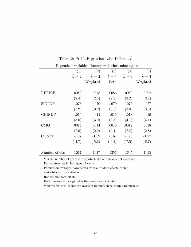
Table 12: Probit Regressions with Di↵erent k
Dependent variable: Dummy = 1 when mine opens
(1) (2) (3) (4) (5)
k = 2 k = 2 k = 3 k = 4 k = 4
Weighted Both Weighted
RPRICE .0080 .0078 .0086 .0089 .0092
(2.4) (2.5) (2.9) (3.2) (3.2)
SIGLNP .073 .070 .070 .075 .077
(3.2) (3.2) (3.3) (3.8) (3.8)
GRINDP .016 .015 .016 .018 .019
(3.0) (3.0) (3.3) (4.1) (4.1)
CMO .0014 .0014 .0016 .0018 .0018
(2.0) (2.0) (2.4) (2.8) (2.8)
CONST -1.37 -1.59 -1.67 -1.90 -1.77
(-4.7) (-5.6) (-6.2) (-7.5) (-6.7)
Number of obs. 1017 1017 1356 1695 1695
k is the number of years during which the option was not exercised
Explanatory variables lagged 2 years
Population averaged parameters from a random e↵ects probit
z–statistics in parentheses
Robust standard errors
Both means that weighted is the same as unweighted
Weights for each choice are ratios of population to sample frequencies
46

Table 13: Baseline Threshold Regressions
Dependent variable: PSTAR
(1) (2) (3) (4)
OLS OLS Corrected Corrected
SIGLNP -1.83 -3.07
(-4.3) (-4.9)
SIGPDP -.231 -.581
(-2.3) (-4.3)
GRINDP -.152 -.141 -.505 -.528
(-1.2) (-1.1) (-3.2) (-3.3)
CMOR -.228 -.238 -.233 -.245
(-13.6) (-13.6) (-8.8) (-9.5)
CONST 72.8 71.2 116.4 116.6
(26.6) (23.5) (38.0) (35.7)
Selection equations
SIGLNP .101
(5.0)
SIGPDP .020
(4.7)
GRINDP .0058 .0068
(1.2) (1.4)
CMOR .0034 .0037
(4.6) (5.0)
Wald test: 281 354
p–value IMR: 0.00 0.00
PSTAR is the price threshold
PSTAR and explanatory variables lagged 2 years
Maximum likelihood estimates
z–statistics in parentheses
Robust standard errors
Corrected means a selectivity correction
Selection equations include instruments and a constant
H0 for Wald test: independent errors
H0 for p–value: no selection
339 observations for threshold equation, 1356 for selection equation
47

Table 14: Thresholds with Regional Fixed E↵ects
Dependent variable: PSTAR
(1) (2)
SIGLNP -1.49
(-2.5)
SIGPDP -.242
(-1.9)
GRINDP -.502 -.505
(-3.8) (-3.7)
CMOR -.236 -.239
(-8.9) (-8.6)
EAST -12.0 -12.2
(-2.5) (-2.5)
SWEST -17.8 -18.5
(-5.5) (-5.5)
WEST -27.5 -27.9
(-6.4) (-6.1)
ALAS -38.8 -39.9
(-7.1) (-7.5)
CONST 120.6 120.5
(42) (39)
PSTAR is the price threshold
PSTAR and explanatory variables lagged 2 years
Correction for sample selection bias
Maximum likelihood estimates
z–statistics in parentheses
Robust standard errors
Base case is the Michigan
339 observations for threshold equation
1356 observations for selection equation
48

Table 15: Thresholds with Mine Characteristics
Dependent variable: PSTAR
(1) (2) (3) (4) (5)
METHOD ORE DEP BYP ALL
SIGLNP -3.28 -2.29 -2.61 -2.47 -1.94
(-5.4) (-3.7) (-4.3) (-4.1) (-3.2)
GRINDP -.417 -.451 -.416 -.461 -.428
(-3.0) (-3.1) (-2.8) (-3.2) (-3.0)
CMOR -.225 -.212 -.223 -.225 -.212
(-7.5) (-9.0) (-8.3) (-9.3) (-7.8)
STRIP -3.65 2.37
(-1.1) (0.7)
SUL -13.9 -9.74
(-5.4) (-3.1)
OX -4.87 -1.58
(-1.9) (-0.6)
POR -10.5 -3.94
(-3.5) (-1.1)
PVR -11.4 -4.79
(-4.6) (-1.7)
MS -5.37 4.66
(-1.2) (1.0)
BYP -12.9 -6.87
(-5.0) (-2.3)
CONST 117.4 120.4 114.7 120.0 115.4
(40) (42) (38) (40) (36)
PSTAR is the price threshold
PSTAR and explanatory variables lagged 2 years
Correction for sample selection bias
Maximum likelihood estimates
z–statistics in parentheses
Robust standard errors
Base case is a Michigan type deposit (UND, NAT, OTH)
339 observations for threshold equation, 1356 for selection equation
49

Table 16: Thresholds with Technological Breakthroughs
Dependent variable: PSTAR
(1) (2) (3)
OPEN FROTH SXEW
SIGLNP -2.67 -3.27 -3.37
(-4.2) (-5.4) (-5,1)
GRINDP -.556 -.462 -.518
(-3.9) (-3.1) (-3.3)
CMOR -.115 -.133 -.235
(-3.1) (-3.3) (-7.0)
OPEN -18.5
(-4.7)
FROTH -15.4
(-3.7)
SX-EW -2.25
(-0.3)
CONST 115.3 115.1 118.4
(42) (39) (40)
PSTAR is the price threshold
PSTAR and explanatory variables lagged 2 years
Correction for sample selection bias
Maximum likelihood estimates
z–statistics in parentheses
Robust standard errors
339 observations for threshold equation, 1356 for selection equation
50

Table 17: Thresholds with Aggregate Economic Events
Dependent variable: PSTAR
(1) (2) (3) (4) (5)
CARTEL WAR DEP PC ALL
SIGLNP -2.98 -3.74 -3.26 -3.34 -3.84
(-4.8) (-6.0) (-5.2) (-5.3) (-5.6)
GRINDP -.527 -.555 -.533 -.504 -.554
(-3.3) (-3.5) (-3.4) (-3.2) (-3.2)
CMOR -.214 -.240 -.237 -.234 -.196
(-7.8) (-7.7) (-8.9) (-8.1) (-5.5)
CARTEL -12.6 -12.7
(-4.0) (-3.6)
WAR -2.74 (-3.07
(-0.7) (-0.8)
DEPRESSION -10.0 -7.29
(-1.3) (-0.8)
CONTROLS -14.4 -11,7
(-1.8) (-1.3)
CONST 118.9 120.9 118.3 118.1 124.4
(40) (36) (40) (40) (35)
PSTAR is the price threshold
PSTAR and explanatory variables lagged 2 years
Correction for sample selection bias
Maximum likelihood estimates
z–statistics in parentheses
Robust standard errors
339 observations for threshold equation, 1356 for selection equation
51
