arX

iv:0

912.

3089

v3 [

cs.N

I] 2

8 Ju

n 20

101

Investment and Pricing with SpectrumUncertainty: A Cognitive Operator’s Perspective

Lingjie Duan, Student Member, IEEE, Jianwei Huang, Member, IEEE, and Biying Shou

Abstract—This paper studies the optimal investment and pricing decisions of a cognitive mobile virtual network operator (C-MVNO)under spectrum supply uncertainty. Compared with a traditional MVNO who often leases spectrum via long-term contracts, a C-MVNOcan acquire spectrum dynamically in short-term by both sensing the empty “spectrum holes” of licensed bands and dynamically leasingfrom the spectrum owner. As a result, a C-MVNO can make flexible investment and pricing decisions to match the current demandsof the secondary unlicensed users. Compared to dynamic spectrum leasing, spectrum sensing is typically cheaper, but the obtaineduseful spectrum amount is random due to primary licensed users’ stochastic traffic. The C-MVNO needs to determine the optimalamounts of spectrum sensing and leasing by evaluating the trade off between cost and uncertainty. The C-MVNO also needs todetermine the optimal price to sell the spectrum to the secondary unlicensed users, taking into account wireless heterogeneity ofusers such as different maximum transmission power levels and channel gains. We model and analyze the interactions between theC-MVNO and secondary unlicensed users as a Stackelberg game. We show several interesting properties of the network equilibrium,including threshold structures of the optimal investment and pricing decisions, the independence of the optimal price on users’ wirelesscharacteristics, and guaranteed fair and predictable QoS among users. We prove that these properties hold for general SNR regimeand general continuous distributions of sensing uncertainty. We show that spectrum sensing can significantly improve the C-MVNO’sexpected profit and users’ payoffs.

Index Terms—Cognitive radio, spectrum trading, spectrum sensing, dynamic spectrum leasing, spectrum pricing, Stackelberg game,Subgame Perfect equilibrium.

✦

1 INTRODUCTION

W IRELESS spectrum is typically considered as ascarce resource, and is traditionally allocated

through static licensing. Field measurements show that,however, most spectrum bands are often under-utilizedeven in densely populated urban areas ( [2]). To achievemore efficient spectrum utilization, people have pro-posed various dynamic spectrum access approaches in-cluding hierarchical-access and dynamic exclusive use( [3]–[7]). Hierarchical-access allows a secondary (unli-censed) network operator or users to opportunisticallyaccess the spectrum without affecting the normal oper-ation of the spectrum owner who serves the primary(licensed) users. Dynamic exclusive use allows a spec-trum owner to dynamically transfer and trade the usageright of its licensed spectrum to a third party (e.g., asecondary network operator or a secondary end-user) inthe spectrum market. This paper considers a secondaryoperator who obtains spectrum resource via both spec-trum sensing as in the hierarchical-access approach anddynamic spectrum leasing as in the dynamic exclusive useapproach.

• Lingjie Duan and Jianwei Huang are with the Department of InformationEngineering, The Chinese University of Hong Kong, Hong Kong.E-mail: {dlj008, jwhuang}@ie.cuhk.edu.hk.

• Biying Shou is with the Department of Management Sciences, CityUniversity of Hong Kong, Hong Kong. E-mail: biying.shou@cityu.edu.hk.

Part of the results has appeared in IEEE INFOCOM, San Diego, USA, March2010 [1].

Spectrum sensing obtains awareness of the spectrumusage and existence of primary users, by using geoloca-tion and database, beacons, or cognitive radios (e.g., [8]–[11]). The primary users are oblivious to the presence ofsecondary cognitive network operators or users. The sec-ondary network operator or users can sense and utilizethe unused “spectrum holes” in the licensed spectrumwithout violating the usage rights of the primary users(e.g., [4], [7]). Since the secondary operator or users doesnot know the primary users’ activities before sensing, theamount of useful spectrum obtained through sensing isuncertain (e.g. [12]–[15]).

With dynamic spectrum leasing, a spectrum ownerallows secondary users to operate in their temporarilyunused part of spectrum in exchange of economic return(e.g., [5], [7], [16]). The dynamic spectrum leasing can beshort-term or even real-time (e.g., [17]–[19]), and can beat a similar time scale of the spectrum sensing operation.

In this paper, we study the operation of a cognitiveradio network that consists a cognitive mobile virtualnetwork operator (C-MVNO) and a group of secondaryunlicensed users. The word “virtual” refers to the factthat the operator does not own the wireless spectrumbands or even the physical network infrastructure. TheC-MVNO serves as the interface between the spectrumowner and the secondary end-users. The word “cog-nitive” refers to the fact that the operator can obtainspectrum resource through both spectrum sensing usingthe cognitive radio technology and dynamic spectrumleasing from the spectrum owner. The operator then

2

resells the obtained spectrum (bandwidth) to secondaryusers to maximize its profit. The proposed model is ahybrid of the hierarchical-access and dynamic exclusiveuse models. It is applicable in various network sce-narios, such as achieving efficient utilization of the TVspectrum in IEEE 802.22 standard [20]. This standardsuggests that the secondary system should operate on apoint-to-multipoint basis, i.e., the communications willhappen between secondary base stations and secondarycustomer-premises equipment. The base stations can beoperated by one or several C-MVNOs introduced in thispaper.

Compared with a traditional MVNO who only leasesspectrum through long-term contracts, a C-MVNO candynamically adjust its sensing and leasing decisions tomatch the changes of users’ demand at a short time scale.Moreover, sensing often offers a cheaper way to obtainspectrum compared with leasing. The cost of sensingmainly includes the sensing time and energy, and doesnot include explicit cost paid to the spectrum owner.With a mature spectrum sensing technology, sensing costshould be reasonable low (otherwise there is no pointof using cognitive radio). Spectrum leasing, however,involves direct negotiation with the spectrum owner.When the spectrum owner determines the cost of leasing,it needs to calculate its opportunity cost, i.e., how muchrevenue the spectrum can provide if the spectrum ownerprovides services directly over it. It is reasonable tobelieve that the leasing cost is more expensive than thesensing cost in most cases1. Although sensing is cheaper,the amount of spectrum obtained through sensing isoften uncertain due to the stochastic nature of primaryusers’ traffic. It is thus critical for a C-MVNO to find theright balance between cost and uncertainty.

Our key results and contributions are summarizedas follows. For simplicity, we refer to the C-MVNO as“operator”, secondary users as “users”, and “dynamicleasing” as “leasing”.

• A Stackelberg game model: We model and analyzethe interactions between the operator and the usersin the spectrum market as a Stackelberg game. Asthe leader, the operator makes the sensing, leasing,and pricing decisions sequentially. As the followers,users then purchase bandwidth from the operatorto maximize their payoffs. By using backward in-duction, we prove the existence and uniquenessof the equilibrium, and show how various systemparameters (i.e., sensing and leasing costs, users’transmission power and channel conditions) affectthe equilibrium behavior.

• Threshold structures of the optimal investment andpricing decisions: At the equilibrium, the operatorwill sense the spectrum only if the sensing costis cheaper than a threshold. Furthermore, it willlease some spectrum only if the resource obtained

1. The analysis of this paper also covers the case where sensing ismore expensive than leasing, which is a trivial case to study.

through sensing is below a threshold. Finally, theoperator will charge a constant price to the users ifthe total bandwidth obtained through sensing andleasing does not exceed a threshold. The thresholdsare easy to compute and the corresponding deci-sions rules are easy to implement in practice.

• Fair and predictable QoS: The operator’s optimal pric-ing decision is independent of the users’ wirelesscharacteristics. Each user receives a payoff that isproportional to its channel gain and transmissionpower, which leads to the same signal-to-noise(SNR) for all users.

• Impact of spectrum sensing: We show that the avail-ability of sensing always increases the operator’sprofit in the expected sense. The actual realizationof the profit at a particular time heavily dependson the spectrum sensing results. Users always getbetter payoffs when the operator performs spectrumsensing.

Section 2 introduces the network model and prob-lem formulation. In Section 3, we analyze the gamemodel through backward induction. We discuss variousinsights obtained from the equilibrium analysis andpresent some numerical results in Section 4. In Section5, we show the impact of spectrum sensing on both theoperator and users. We conclude in Section 6 and outlinesome future research directions.

1.1 Related Work

There is a growing interest in studying the investmentand pricing decisions of cognitive network operatorsrecently. Several auction mechanisms have been pro-posed to study the investment problems of cognitivenetwork operators (e.g., [21], [22]). Other recent resultsstudied the pricing decisions of the cognitive networkoperators who interact with a group of secondary users(e.g., [23]–[30]). [21] considered users’ queueing delaysand obtained most results through simulations. [23] pre-sented a recent survey on the spectrum sharing gamesof network operators and cognitive radio networks.[24] studied the competition among multiple serviceproviders without modeling users’ wireless details. [25]considered a pricing competition game of two operatorsand adopted a simplified wireless model for the users.[26] derived users’ demand functions based on the ac-ceptance probability model for the users. [27] exploreddemand functions based on both quality-sensitive andprice-sensitive buyer population models. [28] formulatedthe interaction between one primary user (monopolist)and multiple secondary users as a Stackelberg game.The primary user uses some secondary users as re-lays and leases its bandwidth to those relays to collectrevenue. [29] studied a multiple-level spectrum marketamong primary, secondary, and tertiary services whereglobal information is not available. [30] considered theshort-term spectrum trading between multiple primaryusers and multiple secondary users. The spectrum buy-

3

Spectrum Owner’s Service Band Spectrum Owner’s Transference Band

Channels PUs’ Activity Band Operator’s Sensed Band Operator’s Leased Band

1t

( )f HZ

2t

1 2 3 4 5 6 7 8 9 10 111213141516171819202122232425262728293031323334

Fig. 1. Operator’s Investment in Spectrum Sensing andLeasing

ing behaviors of secondary users are modeled as anevolutionary game, while selling behaviors of primaryusers are modeled as a noncooperative game. [26]–[30]obtained most interesting results through simulations.There are only few papers (e.g., [19], [29], [31]) thatjointly considered the spectrum investment and servicepricing problem as this paper. None of the above workconsidered the impact of supply uncertainty due tospectrum sensing.

Our model of spectrum uncertainty is related to therandom-yield model in supply chain management (e.g.,[32]–[34]). The unique wireless aspects of the systemmodel lead to new solutions and insights in our problem.

Our paper represents a first attempt of understandinghow spectrum uncertainty impacts the economic deci-sions of an cognitive radio operator. To obtain sharpinsights, we focus on a stylized model where a monopo-list operator faces a group of secondary users. There aremany more interesting research issues in this area. Someare further discussed in Section 6.

2 NETWORK MODEL

2.1 Background on Spectrum Sensing and Leasing

To illustrate the opportunity and trade-off of spectrumsensing and leasing, we consider a spectrum owner whodivides its licensed spectrum into two types:

• Service Band: This band is reserved for serving thespectrum owner’s primary users (PUs). Since thePUs’ traffic is stochastic, there will be some unusedspectrum which changes dynamically. The operatorcan sense and utilize the unused portions. There areno explicit communications between the spectrumowner and the operator.

• Transference Band: The spectrum owner temporarilydoes not use this band. The operator can lease thebandwidth through explicit communications withthe spectrum owner. No sensing is allowed in thisband.

Due to the short-term property of both sensing andleasing, the operator needs to make both the sensing andleasing decisions in each time slot.

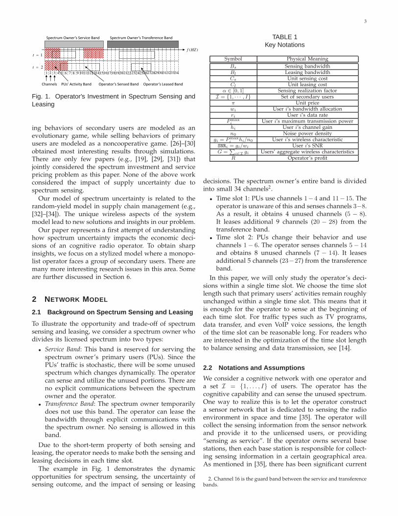
The example in Fig. 1 demonstrates the dynamicopportunities for spectrum sensing, the uncertainty ofsensing outcome, and the impact of sensing or leasing

TABLE 1Key Notations

Symbol Physical Meaning

Bs Sensing bandwidthBl Leasing bandwidthCs Unit sensing costCl Unit leasing cost

α ∈ [0, 1] Sensing realization factorI = {1, · · · , I} Set of secondary users

π Unit pricewi User i’s bandwidth allocationri User i’s data rate

Pmaxi

User i’s maximum transmission powerhi User i’s channel gainn0 Noise power density

gi = Pmaxi

hi/n0 User i’s wireless characteristicSNRi = gi/wi User i’s SNRG =

∑

i∈Igi Users’ aggregate wireless characteristics

R Operator’s profit

decisions. The spectrum owner’s entire band is dividedinto small 34 channels2.

• Time slot 1: PUs use channels 1−4 and 11−15. Theoperator is unaware of this and senses channels 3−8.As a result, it obtains 4 unused channels (5 − 8).It leases additional 9 channels (20 − 28) from thetransference band.

• Time slot 2: PUs change their behavior and usechannels 1− 6. The operator senses channels 5− 14and obtains 8 unused channels (7 − 14). It leasesadditional 5 channels (23−27) from the transferenceband.

In this paper, we will only study the operator’s deci-sions within a single time slot. We choose the time slotlength such that primary users’ activities remain roughlyunchanged within a single time slot. This means that itis enough for the operator to sense at the beginning ofeach time slot. For traffic types such as TV programs,data transfer, and even VoIP voice sessions, the lengthof the time slot can be reasonable long. For readers whoare interested in the optimization of the time slot lengthto balance sensing and data transmission, see [14].

2.2 Notations and Assumptions

We consider a cognitive network with one operator anda set I = {1, . . . , I} of users. The operator has thecognitive capability and can sense the unused spectrum.One way to realize this is to let the operator constructa sensor network that is dedicated to sensing the radioenvironment in space and time [35]. The operator willcollect the sensing information from the sensor networkand provide it to the unlicensed users, or providing“sensing as service”. If the operator owns several basestations, then each base station is responsible for collect-ing sensing information in a certain geographical area.As mentioned in [35], there has been significant current

2. Channel 16 is the guard band between the service and transferencebands.

4

�Stage I: Operator determines sensing amount ��

realize available

bandwidth ���

Stage II: Operator determines leasing amount ��

Stage III: Operator announces price � to market

Stage IV: End-users determine the demands for

bandwidth from the operator

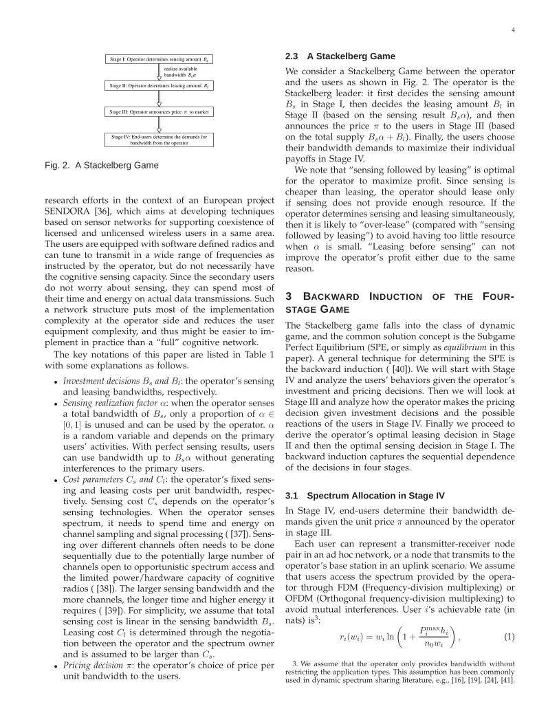
Fig. 2. A Stackelberg Game

research efforts in the context of an European projectSENDORA [36], which aims at developing techniquesbased on sensor networks for supporting coexistence oflicensed and unlicensed wireless users in a same area.The users are equipped with software defined radios andcan tune to transmit in a wide range of frequencies asinstructed by the operator, but do not necessarily havethe cognitive sensing capacity. Since the secondary usersdo not worry about sensing, they can spend most oftheir time and energy on actual data transmissions. Sucha network structure puts most of the implementationcomplexity at the operator side and reduces the userequipment complexity, and thus might be easier to im-plement in practice than a “full” cognitive network.

The key notations of this paper are listed in Table 1with some explanations as follows.

• Investment decisions Bs and Bl: the operator’s sensingand leasing bandwidths, respectively.

• Sensing realization factor α: when the operator sensesa total bandwidth of Bs, only a proportion of α ∈[0, 1] is unused and can be used by the operator. αis a random variable and depends on the primaryusers’ activities. With perfect sensing results, userscan use bandwidth up to Bsα without generatinginterferences to the primary users.

• Cost parameters Cs and Cl: the operator’s fixed sens-ing and leasing costs per unit bandwidth, respec-tively. Sensing cost Cs depends on the operator’ssensing technologies. When the operator sensesspectrum, it needs to spend time and energy onchannel sampling and signal processing ( [37]). Sens-ing over different channels often needs to be donesequentially due to the potentially large number ofchannels open to opportunistic spectrum access andthe limited power/hardware capacity of cognitiveradios ( [38]). The larger sensing bandwidth and themore channels, the longer time and higher energy itrequires ( [39]). For simplicity, we assume that totalsensing cost is linear in the sensing bandwidth Bs.Leasing cost Cl is determined through the negotia-tion between the operator and the spectrum ownerand is assumed to be larger than Cs.

• Pricing decision π: the operator’s choice of price perunit bandwidth to the users.

2.3 A Stackelberg Game

We consider a Stackelberg Game between the operatorand the users as shown in Fig. 2. The operator is theStackelberg leader: it first decides the sensing amountBs in Stage I, then decides the leasing amount Bl inStage II (based on the sensing result Bsα), and thenannounces the price π to the users in Stage III (basedon the total supply Bsα + Bl). Finally, the users choosetheir bandwidth demands to maximize their individualpayoffs in Stage IV.

We note that “sensing followed by leasing” is optimalfor the operator to maximize profit. Since sensing ischeaper than leasing, the operator should lease onlyif sensing does not provide enough resource. If theoperator determines sensing and leasing simultaneously,then it is likely to “over-lease” (compared with “sensingfollowed by leasing”) to avoid having too little resourcewhen α is small. “Leasing before sensing” can notimprove the operator’s profit either due to the samereason.

3 BACKWARD INDUCTION OF THE FOUR-STAGE GAME

The Stackelberg game falls into the class of dynamicgame, and the common solution concept is the SubgamePerfect Equilibrium (SPE, or simply as equilibrium in thispaper). A general technique for determining the SPE isthe backward induction ( [40]). We will start with StageIV and analyze the users’ behaviors given the operator’sinvestment and pricing decisions. Then we will look atStage III and analyze how the operator makes the pricingdecision given investment decisions and the possiblereactions of the users in Stage IV. Finally we proceed toderive the operator’s optimal leasing decision in StageII and then the optimal sensing decision in Stage I. Thebackward induction captures the sequential dependenceof the decisions in four stages.

3.1 Spectrum Allocation in Stage IV

In Stage IV, end-users determine their bandwidth de-mands given the unit price π announced by the operatorin stage III.

Each user can represent a transmitter-receiver nodepair in an ad hoc network, or a node that transmits to theoperator’s base station in an uplink scenario. We assumethat users access the spectrum provided by the opera-tor through FDM (Frequency-division multiplexing) orOFDM (Orthogonal frequency-division multiplexing) toavoid mutual interferences. User i’s achievable rate (innats) is3:

ri(wi) = wi ln

(1 +

Pmaxi hi

n0wi

), (1)

3. We assume that the operator only provides bandwidth withoutrestricting the application types. This assumption has been commonlyused in dynamic spectrum sharing literature, e.g., [16], [19], [24], [41].

5

where wi is the allocated bandwidth from the operator,Pmaxi is user i’s maximum transmission power, n0 is the

noise power per unit bandwidth, hi is user i’s channelgain (between user i’s own transmitter and receiver inan ad hoc network, or between user i’s transmitter to theoperator’s base station in an uplink scenario). To obtainrate in (1), user i spreads its maximum transmissionpower Pmax

k across the entire allocated bandwidth wi.To simplify the notation, we let gi = Pmax

i hi/n0, thusgi/wi is the user i’s signal-to-noise ratio (SNR). Herewe focus on best-effort users who are interested inmaximizing their data rates. Each user only knows itslocal information (i.e., Pmax

i , hi, and n0) and does notknow anything about other users.

From a user’s point of view, it does not matterwhether the bandwidth has been obtained by the opera-tor through spectrum sensing or dynamic leasing. Eachunit of allocated bandwidth is perfectly reliable for theuser.

To obtain closed-form solutions, we first focus on thehigh SNR regime where SNR ≫ 1. This is motivated by thefact that users often have limited choices of modulationand coding schemes, and thus may not be able to decodea transmission if the SNR is below a threshold. In thehigh SNR regime, the rate in (1) can be approximated as

ri(wi) = wi ln

(giwi

). (2)

Although the analytical solutions in Section 3 are derivedbased on (2), we emphasize that all the major engineeringinsights remain true in the general SNR regime. A formalproof is in Section 4.

A user i’s payoff is a function of the allocated band-width wi and the price π,

ui(π,wi) = wi ln

(giwi

)− πwi, (3)

i.e., the difference between the data rate and the linearpayment (πwi). Payoff ui(π,wi) is concave in wi, and theunique bandwidth demand that maximizes the payoff is

w∗i (π) = arg max

wi≥0ui(π,wi) = gie

−(1+π), (4)

which is always positive, linear in gi, and decreasingin price π. Since gi is linear in channel gain hi andtransmission power Pmax

i , then a user with a betterchannel condition or a larger transmission power hasa larger demand.

Equation (4) shows that each user i achieves the sameSNR:

SNRi =gi

w∗i (π)

= e(1+π).

but a different payoff that is linear in gi,

ui(π,w∗i (π)) = gie

−(1+π).

We denote users’ aggregate wireless characteristics asG =

∑i∈I gi. The users’ total demand is

∑

i∈I

w∗i (π) = Ge−(1+π). (5)

1( )S

2( )S

3( )S

0 1

( )D

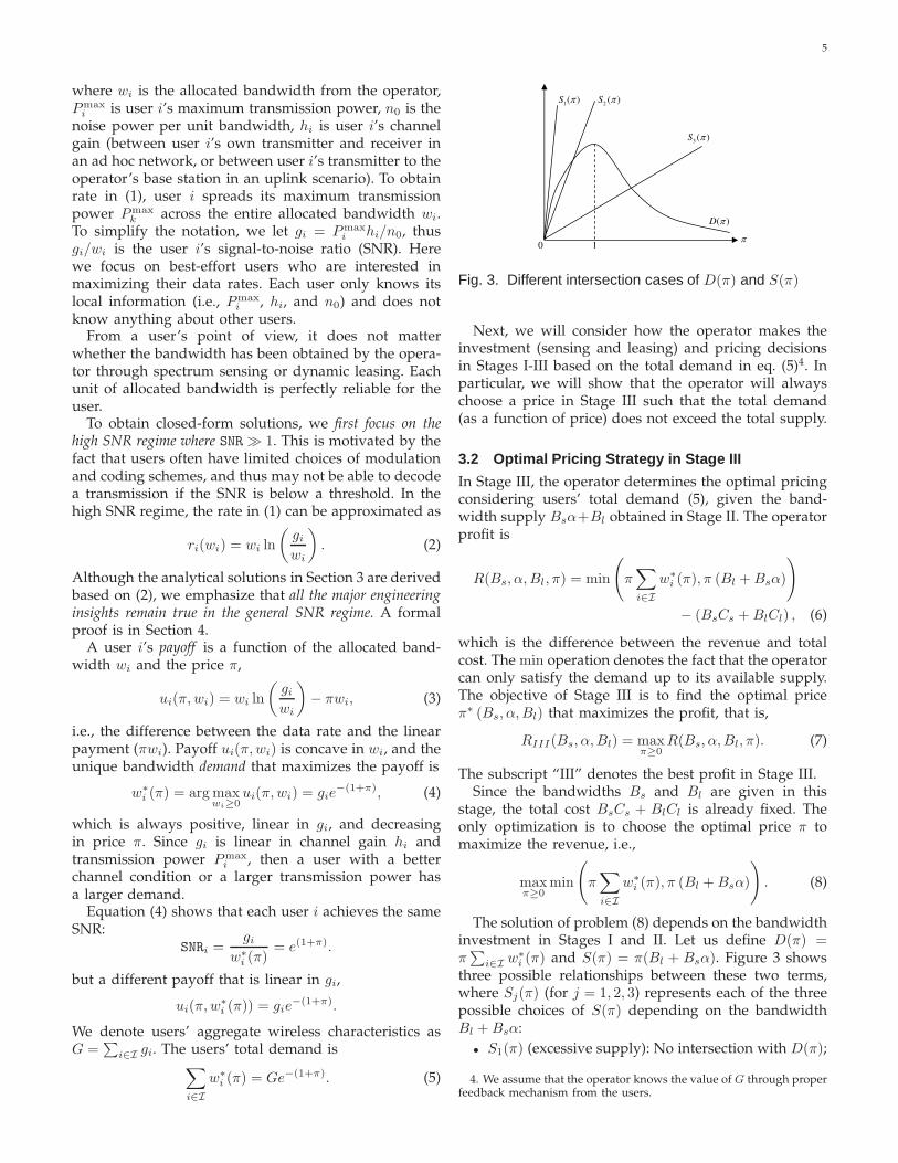
Fig. 3. Different intersection cases of D(π) and S(π)

Next, we will consider how the operator makes theinvestment (sensing and leasing) and pricing decisionsin Stages I-III based on the total demand in eq. (5)4. Inparticular, we will show that the operator will alwayschoose a price in Stage III such that the total demand(as a function of price) does not exceed the total supply.

3.2 Optimal Pricing Strategy in Stage III

In Stage III, the operator determines the optimal pricingconsidering users’ total demand (5), given the band-width supply Bsα+Bl obtained in Stage II. The operatorprofit is

R(Bs, α,Bl, π) = min

(π∑

i∈I

w∗i (π), π (Bl +Bsα)

)

− (BsCs +BlCl) , (6)

which is the difference between the revenue and totalcost. The min operation denotes the fact that the operatorcan only satisfy the demand up to its available supply.The objective of Stage III is to find the optimal priceπ∗ (Bs, α,Bl) that maximizes the profit, that is,

RIII(Bs, α,Bl) = maxπ≥0

R(Bs, α,Bl, π). (7)

The subscript “III” denotes the best profit in Stage III.Since the bandwidths Bs and Bl are given in this

stage, the total cost BsCs + BlCl is already fixed. Theonly optimization is to choose the optimal price π tomaximize the revenue, i.e.,

maxπ≥0

min

(π∑

i∈I

w∗i (π), π (Bl +Bsα)

). (8)

The solution of problem (8) depends on the bandwidthinvestment in Stages I and II. Let us define D(π) =π∑

i∈I w∗i (π) and S(π) = π(Bl + Bsα). Figure 3 shows

three possible relationships between these two terms,where Sj(π) (for j = 1, 2, 3) represents each of the threepossible choices of S(π) depending on the bandwidthBl +Bsα:

• S1(π) (excessive supply): No intersection with D(π);

4. We assume that the operator knows the value of G through properfeedback mechanism from the users.

6

TABLE 2Optimal Pricing Decision and Profit in Stage III

Total Bandwidth Obtained inStages I and II

Optimal Price π∗ (Bs, α, Bl) Optimal Profit RIII(Bs, α,Bl)

Excessive Supply Regime:Bl + Bsα ≥ Ge−2

πES = 1 RES

III(Bs, α,Bl) = Ge−2 − BsCs − BlCl

Conservative Supply Regime:Bl + Bsα < Ge−2

πCS = ln(

G

Bl+Bsα

)

− 1 RCS

III(Bs, α,Bl) = (Bl + Bsα) ln

(

G

Bl+Bsα

)

−

Bs(α + Cs)−Bl(1 + Cl)

• S2(π) (excessive supply): intersect once with D(π)where D(π) has a non-negative slope;

• S3(π) (conservative supply): intersect once withD(π) where D(π) has a negative slope.

In the excessive supply regime,maxπ≥0min (S(π), D(π)) = maxπ≥0 D(π), i.e., themax-min solution occurs at the maximum value of D(π)with π∗ = 1. In this regime, the total supply is largerthan the total demand at the best price choice. In theconservative supply regime, the max-min solution occursat the unique intersection point of D(π) and S(π). Theabove observations lead to the following result.

Theorem 1: The optimal pricing decision and the corre-sponding optimal profit at Stage III can be characterizedby Table 2.

The proof of Theorem 1 is given in Appendix A. Notethat in the excessive supply regime, some bandwidthis left unsold (i.e., S(π∗) > D(π∗)). This is becausethe acquired bandwidth is too large, and selling all thebandwidth will lead to a very low price that decreasesthe revenue (the product of price and sold bandwidth).The profit can be apparently improved if the operatoracquires less bandwidth in Stages I and II. Later analysisin Stages II and I will show that the equilibrium of thegame must lie in the conservative supply regime if thesensing cost is non-negligible.

3.3 Optimal Leasing Strategy in Stage II

In Stage II, the operator decides the optimal leasingamount Bl given the sensing result Bsα:

RII(Bs, α) = maxBl≥0

RIII(Bs, α,Bl). (9)

We decompose problem (9) into two subproblems basedon the two supply regimes in Table 2,

1) Choose Bl to reach the excessive supply regime inStage III:

RESII (Bs, α) = max

Bl≥max{Ge−2−Bsα,0}RES

III(Bs, α,Bl).

(10)2) Choose Bl to reach the conservative supply regime

in Stage III:

RCSII (Bs, α) = max

0≤Bl≤Ge−2−BsαRCS

III(Bs, α,Bl), (11)

To solve subproblems (10) and (11), we need to con-sider the bandwidth obtained from sensing.

• Excessive Supply (Bsα > Ge−2): in this case, thefeasible sets of both subproblems (10) and (11) are

empty. In fact, the bandwidth supply is already inthe excessive supply regime as defined in Table II,and it is optimal not to lease in Stage II.

• Conservative Supply (Bsα ≤ Ge−2): first, we can showthat the unique optimal solution of subproblem (10)is B∗

l = Ge−2 − Bsα. This means that the optimalobjective value of subproblem (10) is no larger thanthat of subproblem (11), and thus it is enough toconsider subproblem (11) in the conservative supplyregime only.

Base on the above observations and some furtheranalysis, we can show the following:

Theorem 2: In Stage II, the optimal leasing decisionand the corresponding optimal profit are summarizedin Table 3.

The proof of Theorem 2 is given in Appendix B. Table3 contains three cases based on the value of Bsα: (CS1),(CS2), and (ES3). The first two cases involve solvingthe subproblem (11) in the conservative supply regime,and the last one corresponds to the excessive supplyregime. Although the decisions in cases (CS2) and (ES3)are the same (i.e., zero leasing amount), we still treatthem separately since the profit expressions are different.

It is clear that we have an optimal threshold leasingpolicy here: the operator wants to achieve a total band-width equal to Ge−(2+Cl) whenever possible. When thebandwidth obtained through sensing is not enough, theoperator will lease additional bandwidth to reach thethreshold; otherwise the operator will not lease.

3.4 Optimal Sensing Strategy in Stage I

In Stage I, the operator will decide the optimal sensingamount to maximize its expected profit by taking the un-certainty of the sensing realization factor α into account.The operator needs to solve the following problem

RI = maxBs≥0

RII (Bs) ,

where RII (Bs) is obtained by taking the expectation ofα over the profit functions in Stage II (i.e., RCS1

II (Bs, α),RCS2

II (Bs, α), and RES3II (Bs, α) in Table 3).

To obtain closed-form solutions, we assume that thesensing realization factor α follows a uniform distri-bution in [0, 1]. In Section 4.1, we prove that the majorengineering insights also hold under any general distribution.

To avoid the trivial case where sensing is so cheapthat it is optimal to sense a huge amount of bandwidth,

7

TABLE 3Optimal Leasing Decision and Profit in Stage II

Given Sensing Result Bsα After Stage I Optimal Leasing Amount B∗l

Optimal Profit RII (Bs, α)

(CS1) Bsα ≤ Ge−(2+Cl) BCS1l

= Ge−(2+Cl) −Bsα RCS1II

(Bs, α) = Ge−(2+Cl) +Bs(αCl − Cs)

(CS2) Bsα ∈(

Ge−(2+Cl), Ge−2]

BCS2l

= 0 RCS2II

(Bs, α) = Bsα ln(

G

Bsα

)

− Bs(α + Cs)

(ES3) Bsα > Ge−2 BES3l

= 0 RES3II

(Bs, α) = Ge−2 − BsCs

0 0.01 0.02 0.03 0.04 0.05 0.060

0.005

0.01

0.015

0.02

0.025

Bs

RII (

Bs )

(Cl,C

s)=(2,0.8)

(Cl,C

s)=(2,1.2)

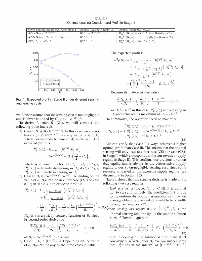
Fig. 4. Expected profit in Stage II under different sensingand leasing costs

we further assume that the sensing cost is non-negligibleand is lower bounded by Cs ≥ (1− e−2Cl)/4.

To derive function RII (Bs), we will consider thefollowing three intervals:

1) Case I: Bs ∈ [0, Ge−(2+Cl)]. In this case, we alwayshave Bsα ≤ Ge−(2+Cl) for any value α ∈ [0, 1],which corresponds to case (CS1) in Table 3. Theexpected profit is

R1II(Bs) =Eα∈[0,1]

[RCS1

II (Bs, α)]

=Ge−(2+Cl) +Bs

(Cl

2− Cs

),

which is a linear function of Bs. If Cs > Cl/2,R1

II(Bs) is linearly decreasing in Bs; if Cs < Cl/2,R1

II(Bs) is linearly increasing in Bs.2) Case II: Bs ∈

(Ge−(2+Cl), Ge−2

]. Depending on the

value of α, Bsα can be in either case (CS1) or case(CS2) in Table 3. The expected profit is

R2II(Bs) =E

α∈[0,Ge

−(2+Cl)

Bs

][RCS1

II (Bs, α)]

+ Eα∈

[Ge

−(2+Cl)

Bs,1][RCS2

II (Bs, α)]

=Bs

2ln

(G

Bs

)−

Bs

4+

Bs

4

(Ge−(2+Cl)

Bs

)2

−BsCs.

R2II(Bs) is a strictly concave function of Bs since

its second-order derivative

∂2R2II(Bs)

∂B2s

=1

2Bs

[(Ge−(2+Cl)

Bs

)2

− 1

]< 0

as Bs > Ge−(2+Cl) in this case.3) Case III: Bs ∈

(Ge−2,∞

). Depending on the value

of α, Bsα can be any of the three cases in Table 3.

The expected profit is

R3II(Bs) =E

α∈[0,Ge

−(2+Cl)

Bs

][RCS1

II (Bs, α)]

+ Eα∈

[Ge

−(2+Cl)

Bs,Ge−2

Bs

][RCS2

II (Bs, α)]

+ Eα∈

[Ge−2

Bs,1] [RES3

II (Bs, α)]

=

(G

e2

)2e−2Cl − 1

4Bs

− BsCs +G

e2.

Because its first-order derivative

∂R3II(Bs)

∂Bs

=

(Ge−2

Bs

)21− e−2Cl

4− Cs < 0,

as Bs > Ge−2 in this case, R3II(Bs) is decreasing in

Bs and achieves its maximum at Bs = Ge−2.

To summarize, the operator needs to maximize

RII(Bs) =

R1II(Bs), if 0 ≤ Bs ≤ Ge−(2+Cl);

R2II(Bs), if Ge−(2+Cl) < Bs ≤ Ge−2;

R3II(Bs), if Bs > Ge−2.

(12)We can verify that Case II always achieves a higher

optimal profit than Case III. This means that the optimalsensing will only lead to either case (CS1) or case (CS2)in Stage II, which corresponds to the conservative supplyregime in Stage III. This confirms our previous intuitionthat equilibrium is always in the conservative supplyregime under a non-negligible sensing cost, since someresource is wasted in the excessive supply regime (seediscussions in Section 3.2).

Table 4 shows that the sensing decision is made in thefollowing two cost regimes:

• High sensing cost regime (Cs > Cl/2): it is optimalnot to sense. Intuitively, the coefficient 1/2 is dueto the uniform distribution assumption of α, i.e., onaverage obtaining one unit of available bandwidththrough sensing costs 2Cs.

• Low sensing cost regime (Cs ∈[1−e−2Cl

4 , Cl

2

]): the

optimal sensing amount BL∗s is the unique solution

to the following equation:

∂R2II(Bs)

∂Bs

=1

2ln

(1

Bs/G

)−3

4−Cs−

(e−(2+Cl)

2Bs/G

)2

= 0.

(13)The uniqueness of the solution is due to the strictconcavity of R2

II(Bs) over Bs. We can further showthat BL∗

s lies in the interval of[Ge−(2+Cl), Ge−2

]

8

TABLE 4Choice of Optimal Sensing Amount in Stage I

Optimal Sensing Decision B∗s Expected Profit RI

High Sensing Cost Regime: Cs ≥ Cl/2 B∗s = 0 RH

I= Ge−(2+Cl)

Low Sensing Cost Regime: Cs ∈[

(1 − e−2Cl )/4, Cl/2]

B∗s = BL∗

s , solution to eq. (13) RL

Iin eq. (14)

and is linear in G. Finally, the operator’s optimalexpected profit is

RLI =

BL∗s

2ln

(G

BL∗s

)−BL∗

s

4+

1

4BL∗s

(G

e2+Cl

)2

−BL∗s Cs.

(14)

Based on these observations, we can show the follow-ing:

Theorem 3: In Stage I, the optimal sensing decisionand the corresponding optimal profit are summarizedin Table 4. The optimal sensing amount B∗

l is linear inG.

Figure 4 shows two possible cases for the functionRII(Bs). The vertical dashed line represents Bs =e−(2+Cl). For illustration purpose, we assume G = 1,Cl = 2, and Cs = {0.8, 1.2}. When the sensing costis large (i.e., Cs = 1.2 > Cl/2), RII(Bs) achieves itsoptimum at Bs = 0 and thus it is optimal not to sense.When the sensing cost is small (i.e., Cs = 0.8 < Cl/2),RII(Bs) achieves its optimum at Bs > e−(2+Cl) and it isoptimal to sense a positive amount of spectrum.

4 EQUILIBRIUM SUMMARY AND NUMERICALRESULTS

Based on the discussions in Section 3, we summarizethe operator’s equilibrium sensing/leasing/pricing de-cisions and the equilibrium resource allocations to theusers in Table 5. Several interesting observations are asfollows.

Observation 1: Both the optimal sensing amount B∗s

(either 0 or BL∗s ) and leasing amount B∗

l are linearin the users’ aggregate wireless characteristics G =∑

i∈I Pmaxi hi/n0.

The linearity enables us to normalize optimal sensingand leasing decisions by users’ aggregate wireless char-acteristics, and study the relationships between the nor-malized optimal decisions and other system parametersas in Figs. 5 and 6.

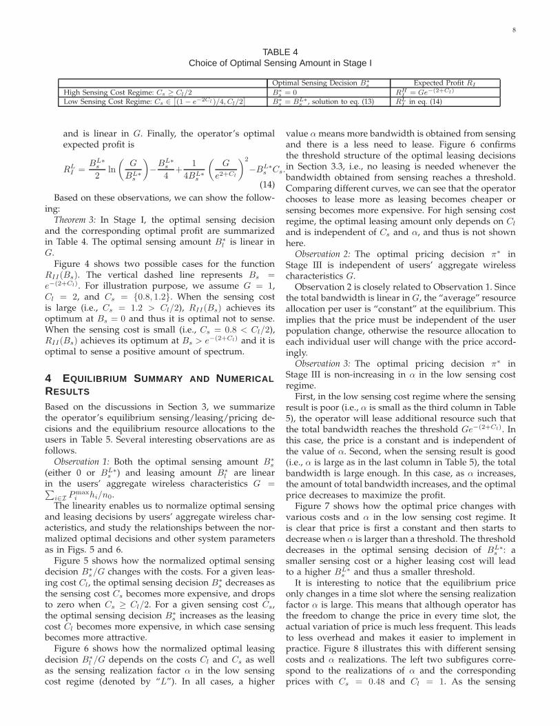
Figure 5 shows how the normalized optimal sensingdecision B∗

s/G changes with the costs. For a given leas-ing cost Cl, the optimal sensing decision B∗

s decreases asthe sensing cost Cs becomes more expensive, and dropsto zero when Cs ≥ Cl/2. For a given sensing cost Cs,the optimal sensing decision B∗

s increases as the leasingcost Cl becomes more expensive, in which case sensingbecomes more attractive.

Figure 6 shows how the normalized optimal leasingdecision B∗

l /G depends on the costs Cl and Cs as wellas the sensing realization factor α in the low sensingcost regime (denoted by “L”). In all cases, a higher

value α means more bandwidth is obtained from sensingand there is a less need to lease. Figure 6 confirmsthe threshold structure of the optimal leasing decisionsin Section 3.3, i.e., no leasing is needed whenever thebandwidth obtained from sensing reaches a threshold.Comparing different curves, we can see that the operatorchooses to lease more as leasing becomes cheaper orsensing becomes more expensive. For high sensing costregime, the optimal leasing amount only depends on Cl

and is independent of Cs and α, and thus is not shownhere.

Observation 2: The optimal pricing decision π∗ inStage III is independent of users’ aggregate wirelesscharacteristics G.

Observation 2 is closely related to Observation 1. Sincethe total bandwidth is linear in G, the “average” resourceallocation per user is “constant” at the equilibrium. Thisimplies that the price must be independent of the userpopulation change, otherwise the resource allocation toeach individual user will change with the price accord-ingly.

Observation 3: The optimal pricing decision π∗ inStage III is non-increasing in α in the low sensing costregime.

First, in the low sensing cost regime where the sensingresult is poor (i.e., α is small as the third column in Table5), the operator will lease additional resource such thatthe total bandwidth reaches the threshold Ge−(2+Cl). Inthis case, the price is a constant and is independent ofthe value of α. Second, when the sensing result is good(i.e., α is large as in the last column in Table 5), the totalbandwidth is large enough. In this case, as α increases,the amount of total bandwidth increases, and the optimalprice decreases to maximize the profit.

Figure 7 shows how the optimal price changes withvarious costs and α in the low sensing cost regime. Itis clear that price is first a constant and then starts todecrease when α is larger than a threshold. The thresholddecreases in the optimal sensing decision of BL∗

s : asmaller sensing cost or a higher leasing cost will leadto a higher BL∗

s and thus a smaller threshold.It is interesting to notice that the equilibrium price

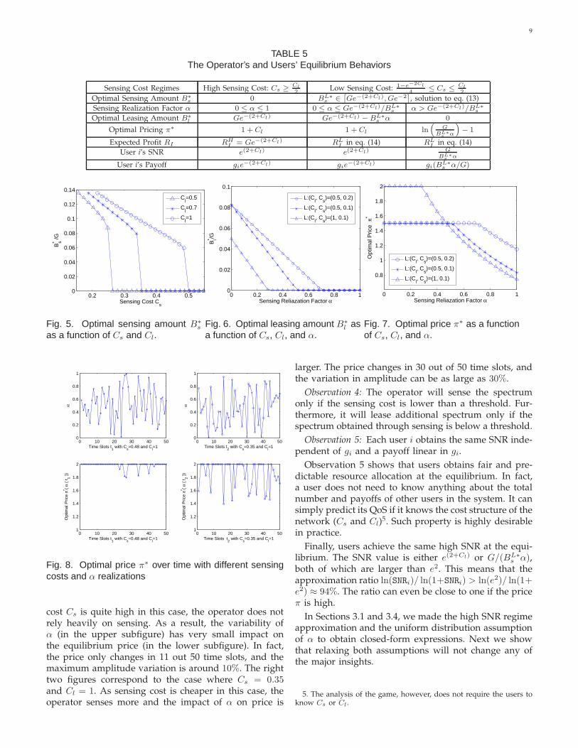
only changes in a time slot where the sensing realizationfactor α is large. This means that although operator hasthe freedom to change the price in every time slot, theactual variation of price is much less frequent. This leadsto less overhead and makes it easier to implement inpractice. Figure 8 illustrates this with different sensingcosts and α realizations. The left two subfigures corre-spond to the realizations of α and the correspondingprices with Cs = 0.48 and Cl = 1. As the sensing

9

TABLE 5The Operator’s and Users’ Equilibrium Behaviors

Sensing Cost Regimes High Sensing Cost: Cs ≥ Cl

2Low Sensing Cost: 1−e

−2Cl

4≤ Cs ≤ Cl

2

Optimal Sensing Amount B∗s 0 BL∗

s ∈[

Ge−(2+Cl), Ge−2]

, solution to eq. (13)

Sensing Realization Factor α 0 ≤ α ≤ 1 0 ≤ α ≤ Ge−(2+Cl)/BL∗s α > Ge−(2+Cl)/BL∗

s

Optimal Leasing Amount B∗l

Ge−(2+Cl) Ge−(2+Cl) − BL∗s α 0

Optimal Pricing π∗ 1 + Cl 1 + Cl ln(

G

BL∗s

α

)

− 1

Expected Profit RI RH

I= Ge−(2+Cl) RL

Iin eq. (14) RL

Iin eq. (14)

User i’s SNR e(2+Cl) e(2+Cl) G

BL∗s

α

User i’s Payoff gie−(2+Cl) gie−(2+Cl) gi(BL∗s α/G)

0.2 0.3 0.4 0.50

0.02

0.04

0.06

0.08

0.1

0.12

0.14

Sensing Cost Cs

Bs* /G

Cl=0.5

Cl=0.7

Cl=1

Fig. 5. Optimal sensing amount B∗s

as a function of Cs and Cl.

0 0.2 0.4 0.6 0.8 10

0.02

0.04

0.06

0.08

0.1

Sensing Reliazation Factor α

Bl* /G

L:(Cl, C

s)=(0.5, 0.2)

L:(Cl, C

s)=(0.5, 0.1)

L:(Cl, C

s)=(1, 0.1)

Fig. 6. Optimal leasing amount B∗l as

a function of Cs, Cl, and α.

0 0.2 0.4 0.6 0.8 1

0.8

1

1.2

1.4

1.6

1.8

2

Sensing Reliazation Factor α

Opt

imal

Pric

eπ

*

L:(Cl, C

s)=(0.5, 0.2)

L:(Cl, C

s)=(0.5, 0.1)

L:(Cl, C

s)=(1, 0.1)

Fig. 7. Optimal price π∗ as a functionof Cs, Cl, and α.

0 10 20 30 40 500

0.2

0.4

0.6

0.8

1

Time Slots t1 with C

s=0.48 and C

l=1

α

0 10 20 30 40 500

0.2

0.4

0.6

0.8

1

Time Slots t2 with C

s=0.35 and C

l=1

α

0 10 20 30 40 501

1.2

1.4

1.6

1.8

2

Time Slots t1 with C

s=0.48 and C

l=1

Opt

imal

Pric

e π

* (α

( t 1 )

)

0 10 20 30 40 501

1.2

1.4

1.6

1.8

2

Time Slots t2 with C

s=0.35 and C

l=1

Opt

imal

Pric

e π

* (α

( t 2 )

)

Fig. 8. Optimal price π∗ over time with different sensingcosts and α realizations

cost Cs is quite high in this case, the operator does notrely heavily on sensing. As a result, the variability ofα (in the upper subfigure) has very small impact onthe equilibrium price (in the lower subfigure). In fact,the price only changes in 11 out 50 time slots, and themaximum amplitude variation is around 10%. The righttwo figures correspond to the case where Cs = 0.35and Cl = 1. As sensing cost is cheaper in this case, theoperator senses more and the impact of α on price is

larger. The price changes in 30 out of 50 time slots, andthe variation in amplitude can be as large as 30%.

Observation 4: The operator will sense the spectrumonly if the sensing cost is lower than a threshold. Fur-thermore, it will lease additional spectrum only if thespectrum obtained through sensing is below a threshold.

Observation 5: Each user i obtains the same SNR inde-pendent of gi and a payoff linear in gi.

Observation 5 shows that users obtains fair and pre-dictable resource allocation at the equilibrium. In fact,a user does not need to know anything about the totalnumber and payoffs of other users in the system. It cansimply predict its QoS if it knows the cost structure of thenetwork (Cs and Cl)

5. Such property is highly desirablein practice.

Finally, users achieve the same high SNR at the equi-librium. The SNR value is either e(2+Cl) or G/(BL∗

s α),both of which are larger than e2. This means that theapproximation ratio ln(SNRi)/ ln(1+SNRi) > ln(e2)/ ln(1+e2) ≈ 94%. The ratio can even be close to one if the priceπ is high.

In Sections 3.1 and 3.4, we made the high SNR regimeapproximation and the uniform distribution assumptionof α to obtain closed-form expressions. Next we showthat relaxing both assumptions will not change any ofthe major insights.

5. The analysis of the game, however, does not require the users toknow Cs or Cl.

10

4.1 Robustness of the Observations

Theorem 4: Observations 1-5 still hold under the gen-eral SNR regime (as in (1)) and any general distributionof α.

Proof: We represent a user i’s payoff function in thegeneral SNR regime,

ui(π,wi) = wi ln

(1 +

giwi

)− πwi. (15)

The optimal demand w∗i (π) that maximizes (15) is

w∗i (π) = gi/Q(π), where Q(π) is the unique positive

solution to F (π,Q) := ln(1 +Q)− Q1+Q

− π = 0. We find

the inverse function of Q(π) to be π(Q) = ln(1+Q)− Q1+Q

.By applying the implicit function theorem, we can obtainthe first-order derivative of function Q(π) over π as

Q′(π) = −∂F (π,Q)/∂π

∂F (π,Q)/∂Q=

(1 +Q(π))2

Q(π), (16)

which is always positive. Hence, Q(π) is increasing in π.User i’s optimal payoff is

ui(π,w∗i (π)) =

giQ(π)

[ln(1 +Q(π))− π]. (17)

As a result, a user’s optimal SNR equals gi/w∗i (π) = Q(π)

and is user-independent. The total demand from all usersequals G/Q(π), and the operator’s investment and pric-ing problem is

R∗ =maxBs≥0

Eα∈[0,1][maxBl≥0

maxπ≥0

(min

(π

G

Q(π), π(Bl +Bsα)

)

−BsCs −BlCl)]. (18)

Define R̃∗ = R∗

G, B̃l = Bl

G, and B̃s = Bs

G. Then solving

(18) is equivalent to solving

R̃∗ =maxB̃s≥0

Eα∈[0,1][maxB̃l≥0

maxπ≥0

(min

(π

Q(π), π(B̃l + B̃sα)

)

− B̃sCs − B̃lCl)]. (19)

In Problem (19), it is clear that the operator’s optimaldecisions on leasing, sensing and pricing do not dependon users’ aggregate wireless characteristics. This is truefor any continuous distribution of α. And a user’soptimal payoff in eq. (17) is linear in gi since Q(π)is independent of users’ wireless characteristics. Thisshows that Observations 1, 2, and 5 hold for the generalSNR regime and any general distribution of α. We canalso show that Observations 3 and 4 hold in the generalcase, with a detailed proof in Appendix C.

5 THE IMPACT OF SPECTRUM SENSING UN-CERTAINTY

The key difference between our model and most existingliterature (e.g., [19], [21], [22], [24], [26], [27]) is thepossibility of obtaining resource through the cheaper butuncertain approach of spectrum sensing. Here we willelaborate the impact of sensing on the performances ofoperator and users by comparing with the baseline case

where sensing is not possible. Note that in the highsensing cost regime it is optimal not to sense, as a result,the performance of the operator and users will be thesame as the baseline case. Hence we will focus on thelow sensing cost regime in Table 5.

Observation 6: The operator’s optimal expected profitalways benefits from the availability of spectrum sensingin the low sensing cost regime.

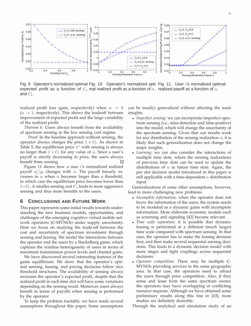
Figure 9 illustrates the normalized optimal expectedprofit as a function of the sensing cost. We assumeleasing cost Cl = 2, and thus the low sensing cost regimecorresponds to the case where Cs ∈ [0.2, 1] in the figure.It is clear that sensing achieves a better optimal expectedprofit in this regime. In fact, sensing leads to 250%increase in profit when Cs = 0.2. The benefit decreases asthe sensing cost becomes higher. When sensing becomestoo expensive, the operator will choose not to sense andthus achieve the same profit as in the baseline case.

Theorem 5: The operator’s realized profit (i.e., theprofit for a given α) is a strictly increasing function in αin the low sensing cost regime. Furthermore, there existsa threshold αth ∈ (0, 1) such that the operator’s realizedprofit is larger than the baseline approach if α > αth.

Proof: As in Table 5, we have two cases in the lowsensing cost regime:

• If α ≤ Ge−(2+Cl)/BL∗s , then substituting BL∗

s intoRCS1

II (Bs, α) in Table 3 leads to the realized profit

RCS1II (α) = Ge−(2+Cl) −BL∗

s Cs +BL∗s αCl,

which is strictly and linearly increasing in α.• If α ≥ Ge−(2+Cl)/BL∗

s , then substituting BL∗s into

RCS2II (Bs, α) in Table 3 leads to the realized profit

RCS2II (α) = BL∗

s α

(ln

(G

BL∗s α

)− 1

)−BL∗

s Cs.

Because the first-order derivative

∂RCS2II (α)

∂α= BL∗

s

(ln

(G

BL∗s α

)− 2

)> 0,

as BL∗s ≤ Ge−2, RCS2

II (α) is strictly increasing in α.

We can also verify that RCS1II (α) = RCS2

II (α) whenα = Ge−(2+Cl)/BL∗

s . Therefore, the realized profit is acontinuous and strictly increasing function of α.

Next we prove the existence of threshold αth. Firstconsider the extreme case α = 0. Since the operator ob-tains no bandwidth through sensing but still incurs somecost, the profit in this case is lower than the baselinecase. Furthermore, we can verify that RCS2

II (1) > RHI in

Table 5, thus the realized profit at α = 1 is always largerthan the baseline case. Together with the continuity andstrictly increasing nature of the realized profit function,we have proven the existence of threshold of αth.

Figure 10 shows the realized profit as a function of αfor different costs. The realized profit is increasing in α inboth cases. The “crossing” feature of the two increasingcurves is because the optimal sensing B∗

s is larger undera cheaper sensing cost (Cs = 0.5), which leads to larger

11

0.2 0.4 0.6 0.8 10.01

0.02

0.03

0.04

0.05

0.06

0.07

Sensing Cost Cs

Nor

mal

ized

Exp

. Pro

fit R

I /G

Cl=2, with sensing

Cl=2, w./o. sensing

Fig. 9. Operator’s normalized optimalexpected profit as a function of Cs

and Cl.

0 0.2 0.4 0.6 0.8 1−0.04

−0.02

0

0.02

0.04

0.06

0.08

0.1

Sensing Realization Factor α

Nor

mal

ized

Rea

lized

Pro

fit R

IICS

1/2 (

α)/

G

Cl=2,C

s=0.8

Cl=2,w./o. sensing

Cl=2, C

s=0.5

Fig. 10. Operator’s normalized opti-mal realized profit as a function of α.

0 0.2 0.4 0.6 0.8 10.01

0.02

0.03

0.04

0.05

0.06

0.07

0.08

Sensing Realization Factor α

Nor

mal

ized

Rea

lized

Pay

off o

f Use

r u i* (α

) /g

i

Cl=2, C

s=0.8

Cl=2, C

s=0.5

Cl=2, w./o. sensing

Fig. 11. User i’s normalized optimalrealized payoff as a function of α.

realized profit loss (gain, respectively) when α → 0(α → 1, respectively). This shows the tradeoff betweenimprovement of expected profit and the large variabilityof the realized profit.

Theorem 6: Users always benefit from the availabilityof spectrum sensing in the low sensing cost regime.

Proof: In the baseline approach without sensing, theoperator always charges the price 1 + Cl. As shown inTable 5, the equilibrium price π∗ with sensing is alwaysno larger than 1 + Cl for any value of α. Since a user’spayoff is strictly decreasing in price, the users alwaysbenefit from sensing.

Figure 11 shows how a user i’s normalized realizedpayoff u∗

i /gi changes with α. The payoff linearly in-creases in α when α becomes larger than a threshold,in which case the equilibrium price becomes lower than1+Cl. A smaller sensing cost Cs leads to more aggressivesensing and thus more benefits to the users.

6 CONCLUSIONS AND FUTURE WORK

This paper represents some initial results towards under-standing the new business models, opportunities, andchallenges of the emerging cognitive virtual mobile net-work operators (C-MVNOs) under supply uncertainty.Here we focus on studying the trade-off between thecost and uncertainty of spectrum investment throughsensing and leasing. We model the interactions betweenthe operator and the users by a Stackelberg game, whichcaptures the wireless heterogeneity of users in terms ofmaximum transmission power levels and channel gains.

We have discovered several interesting features of thegame equilibrium. We show that the operator’s opti-mal sensing, leasing, and pricing decisions follow nicethreshold structures. The availability of sensing alwaysincreases the operator’s expected profit, despite that therealized profit in each time slot will have some variationsdepending on the sensing result. Moreover, users alwaysbenefit in terms of payoffs when sensing is performedby the operator.

To keep the problem tractable, we have made severalassumptions throughout this paper. Some assumptions

can be (easily) generalized without affecting the maininsights.

• Imperfect sensing: we can incorporate imperfect spec-trum sensing (i.e., miss-detection and false-positive)into the model, which will change the uncertainty ofthe spectrum sensing. Given that our results workfor any distribution of the sensing realization α, it islikely that such generalization does not change themajor insights.

• Learning: we can also consider the interactions ofmultiple time slots, where the sensing realizationsof previous time slots can be used to update thedistributions of α in future time slots. Again, theper slot decision model introduced in this paper isstill applicable with a time-dependent α distributioninput.

Generalizations of some other assumptions, however,lead to more challenging new problems.

• Incomplete information: when the operator does notknow the information of the users, the system needsto be modeled as a dynamic game with incompleteinformation. More elaborate economic models suchas screening and signaling [42] become relevant.

• Time scale separation: it is possible that dynamicleasing is performed at a different (much larger)time scale compared with spectrum sensing. In thatcase, the operator has to make the leasing decisionfirst, and then make several sequential sensing deci-sions. This leads to a dynamic decision model withmore stages and tight couplings across sequentialdecisions.

• Operator competition: There may be multiple C-MVNOs providing services in the same geographicarea. In that case, the operators need to attractthe users through price competition. Also, if theysense and lease from the same spectrum owner,the operators may have overlapping or conflictingresource requests. Although we have obtained somepreliminary results along this line in [43], morestudies are definitely desirable.

Through the analytical and simulation study of an

12

idealized model in this paper, we have obtained vari-ous interesting engineering and economical insights intothe operations of C-MVNOs. We hope that this papercan contribute to the further understanding of propernetwork architecture decisions and business models offuture cognitive radio systems.

APPENDIX APROOF OF THEOREM 1Given the total bandwidth Bl + Bsα, the objective ofStage III is to solve the optimization problem (8), i.e.,maxπ≥0min(D(π), S(π)). First, by examining the deriva-tive of D(π), i.e., ∂D(π)/∂π = (1 − π)Ge−(1+π), we cansee that the continuous function D(π) is increasing inπ ∈ [0, 1] and decreasing in π ∈ [1,+∞], and D(π) ismaximized when π = 1. Since S(π) always increases inπ and D(π) is concave over π ∈ [0, 1], S(π) intersects

with D(π) if and only if ∂D(π)∂π

> ∂S(π)∂π

at π = 0, i.e.,Bl +Bsα < Ge−1.

Next we divide our discussion into the intersectioncase and the non-intersection case:

1) Given Bl+Bsα ≤ Ge−1, S(π) intersects with D(π).By solving equation S(π) = D(π) the intersection

point is π = ln(

GBl+Bsα

)− 1. There are two sub-

cases:

• when Bl + Bsα ≤ Ge−2, S(π) intersects withD(π), and min(D(π), S(π)) is maximized at the

intersection point, i.e., π∗ = ln(

GBl+Bsα

)− 1.

(See S3(π) in Fig. 3.)• when Bl + Bsα ≥ Ge−2, S(π) intersects with

D(π), and min(D(π), S(π)) is maximized at themaximum value of D(π), i.e., π∗ = 1. (See S2(π)in Fig. 3.)

2) Given Bl+Bsα ≥ Ge−1, S(π) doesn’t intersect withD(π). Then min(D(π), S(π)) is maximized at themaximum value of D(π), i.e., π∗ = 1. (See S1(π) inFig. 3.)

APPENDIX BPROOF OF THEOREM 2Given the sensing result Bsα, the objective of StageII is to solve the decomposed two subproblems (10)and (11), and select the best one with better optimalperformance. Since RES

III(Bs, α,Bl) in subproblem (10)is linearly decreasing in Bl, its optimal solution alwayslies at the lower boundary of the feasible set (i.e., B∗

l =max{Ge−2−Bsα, 0}). We compare the optimal profits oftwo subproblems (i.e., RES

II (Bs, α) and RCSII (Bs, α)) for

different sensing results:

1) Given Bsα > Ge−2, the obtained bandwidth afterStage I is already in excessive supply regime. Thusit is optimal not to lease for subproblem (10) (i.e.,BES3

l = 0 of case (ES3) in Table 3).2) Given 0 ≤ Bsα ≤ Ge−2, the optimal leasing deci-

sion for subproblem (11) is B∗l = Ge−2 − Bsα and

we have RESIII(Bs, α,Bl) = RCS

III(Bs, α,Bl) whenBl = Ge−2 −Bsα, thus the optimal objective valueof (10) is always no larger than that of (11) and it isenough to consider the conservative supply regimeonly. Since

∂2RCSIII(Bs, α,Bl)

∂B2l

= −1

Bl +Bsα< 0,

RCSIII(Bs, α,Bl) is concave in 0 ≤ Bl ≤ Ge−2 −Bsα.

Thus it is enough to examine the first-order condi-tion

∂RCSIII(Bs, α,Bl)

∂Bl

= ln

(G

Bl +Bsα

)− 2− Cl = 0,

and the boundary condition 0 ≤ Bl ≤ Ge−2 −Bsα.This results in optimal leasing decision B∗

l =max(Ge−(2+Cl) − Bsα, 0) and leads to BCS1

l =Ge−(2+Cl) −Bsα and BCS2

l = 0 of cases (CS1) and(CS2) in Table 3.

By substituting BCS1l and BCS2

l into RCSIII(Bs, α,Bl)

in Table 2, we derive the corresponding optimal profitsRCS1

II (Bs, α) and RCS2II (Bs, α) in Table 3. RES3

II (Bs, α)can also be obtained by substituting BES3

l intoRES

III(Bs, α,Bl).

APPENDIX CSUPPLEMENTARY PROOF OF THEOREM 4In this section, we prove that Observations 3 and 4hold for the genera case (i.e., the general SNR regimeand a general distributions of α). We first show thatObservation 4 holds for the general case.

C.1 Threshold structure of sensing

It is not difficult to show that if the sensing cost ismuch larger than the leasing cost, the operator hasno incentive to sense but will directly lease. Thus thethreshold structure on the sensing decision in Stage I stillholds for the general case. We ignore the details due tospace limitations.

C.2 Threshold structure of leasing

Next we show the threshold structure on leasing in StageII also holds. Similar as in the proof of Theorem 1, wedefine D(π) = π G

Q(π) and S(π) = π(Bsα+Bl).

• We first show that D(π) is increasing when π ∈[0, 0.468] and decreasing when π ∈ [0.468,+∞). Tosee this, we take the first-order derivative of D(π)over π,

D′(π) =2Q(π)2 +Q(π)− (1 +Q(π))2 ln(1 +Q(π))

Q(π)3,

which is positive when Q(π) ∈ [0, 2.163) and nega-tive when Q(π) ∈ [2.163,+∞). Since eq. (16) showsthat Q(π) is increasing in π and π(Q) |Q=2.163=0.468, as a result D(π) is increasing in π ∈ [0, 0.468]

13

1( )S

0 0.468

2( )S

1thB

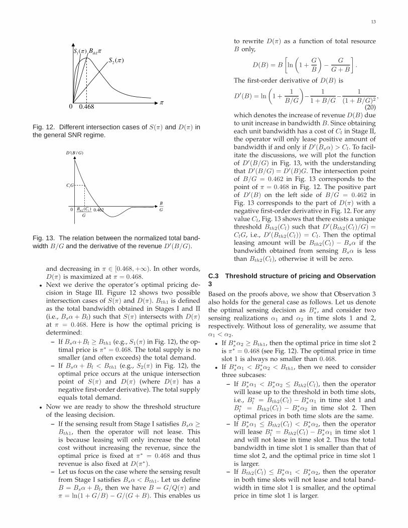
Fig. 12. Different intersection cases of S(π) and D(π) inthe general SNR regime.

0.4622( )

th lB C

G

B

G

lC G

'( / )D B G

0

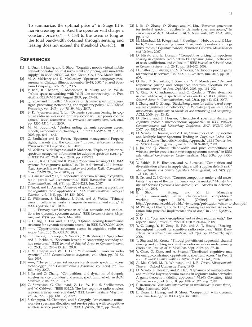
Fig. 13. The relation between the normalized total band-width B/G and the derivative of the revenue D′(B/G).

and decreasing in π ∈ [0.468,+∞). In other words,D(π) is maximized at π = 0.468.

• Next we derive the operator’s optimal pricing de-cision in Stage III. Figure 12 shows two possibleintersection cases of S(π) and D(π). Bth1 is definedas the total bandwidth obtained in Stages I and II(i.e., Bsα + Bl) such that S(π) intersects with D(π)at π = 0.468. Here is how the optimal pricing isdetermined:

– If Bsα+Bl ≥ Bth1 (e.g., S1(π) in Fig. 12), the op-timal price is π∗ = 0.468. The total supply is nosmaller (and often exceeds) the total demand.

– If Bsα + Bl < Bth1 (e.g., S2(π) in Fig. 12), theoptimal price occurs at the unique intersectionpoint of S(π) and D(π) (where D(π) has anegative first-order derivative). The total supplyequals total demand.

• Now we are ready to show the threshold structureof the leasing decision.

– If the sensing result from Stage I satisfies Bsα ≥Bth1, then the operator will not lease. Thisis because leasing will only increase the totalcost without increasing the revenue, since theoptimal price is fixed at π∗ = 0.468 and thusrevenue is also fixed at D(π∗).

– Let us focus on the case where the sensing resultfrom Stage I satisfies Bsα < Bth1. Let us defineB = Bsα + Bl, then we have B = G/Q(π) andπ = ln(1 +G/B) − G/(G + B). This enables us

to rewrite D(π) as a function of total resourceB only,

D(B) = B

[ln

(1 +

G

B

)−

G

G+B

].

The first-order derivative of D(B) is

D′(B) = ln

(1 +

1

B/G

)−

1

1 +B/G−

1

(1 +B/G)2,

(20)which denotes the increase of revenue D(B) dueto unit increase in bandwidth B. Since obtainingeach unit bandwidth has a cost of Cl in Stage II,the operator will only lease positive amount ofbandwidth if and only if D′(Bsα) > Cl. To facil-itate the discussions, we will plot the functionof D′(B/G) in Fig. 13, with the understandingthat D′(B/G) = D′(B)G. The intersection pointof B/G = 0.462 in Fig. 13 corresponds to thepoint of π = 0.468 in Fig. 12. The positive partof D′(B) on the left side of B/G = 0.462 inFig. 13 corresponds to the part of D(π) with anegative first-order derivative in Fig. 12. For anyvalue Cl, Fig. 13 shows that there exists a uniquethreshold Bth2(Cl) such that D′(Bth2(Cl)/G) =ClG, i.e., D′(Bth2(Cl)) = Cl. Then the optimalleasing amount will be Bth2(Cl) − Bsα if thebandwidth obtained from sensing Bsα is lessthan Bth2(Cl), otherwise it will be zero.

C.3 Threshold structure of pricing and Observation3

Based on the proofs above, we show that Observation 3also holds for the general case as follows. Let us denotethe optimal sensing decision as B∗

s , and consider twosensing realizations α1 and α2 in time slots 1 and 2,respectively. Without loss of generality, we assume thatα1 < α2.

• If B∗sα2 ≥ Bth1, then the optimal price in time slot 2

is π∗ = 0.468 (see Fig. 12). The optimal price in timeslot 1 is always no smaller than 0.468.

• If B∗sα1 < B∗

sα2 < Bth1, then we need to considerthree subcases:

– If B∗sα1 < B∗

sα2 ≤ Bth2(Cl), then the operatorwill lease up to the threshold in both time slots,i.e., B∗

l = Bth2(Cl) − B∗sα1 in time slot 1 and

B∗l = Bth2(Cl) − B∗

sα2 in time slot 2. Thenoptimal prices in both time slots are the same.

– If B∗sα1 ≤ Bth2(Cl) < B∗

sα2, then the operatorwill lease B∗

l = Bth2(Cl) − B∗sα1 in time slot 1

and will not lease in time slot 2. Thus the totalbandwidth in time slot 1 is smaller than that oftime slot 2, and the optimal price in time slot 1is larger.

– If Bth2(Cl) ≤ B∗sα1 < B∗

sα2, then the operatorin both time slots will not lease and total band-width in time slot 1 is smaller, and the optimalprice in time slot 1 is larger.

14

To summarize, the optimal price π∗ in Stage III isnon-increasing in α. And the operator will charge aconstant price (π∗ = 0.468) to the users as long asthe total bandwidth obtained through sensing andleasing does not exceed the threshold Bth2(Cl).

REFERENCES

[1] L. Duan, J. Huang, and B. Shou, “Cognitive mobile virtual mobilenetwork operator: optimal investment and pricing with unreliablesupply,” in IEEE INFOCOM, San Diego, CA, USA, March 2010.

[2] M. A. McHenry and D. McCloskey, “Spectrum occupancy mea-surements: Chicago, illinois, november 16-18, 2005,” Shared Spec-trum Company, Tech. Rep., 2005.

[3] P. Bahl, R. Chandra, T. Moscibroda, R. Murty, and M. Welsh,“White space networking with Wi-Fi like connectivity,” in Proc.ACM SIGCOMM 2009, August 2009, pp. 27–38.

[4] Q. Zhao and B. Sadler, “A survey of dynamic spectrum access:signal processing, networking, and regulatory policy,” IEEE SignalProcessing, vol. 24(3), pp. 78–89, May 2007.

[5] S. K. Jayaweera and T. Li, “Dynamic spectrum leasing in cog-nitive radio networks via primary-secondary user power controlgames,” IEEE Transactions on Wireless Communications, vol. 8(6),pp. 3300–3310, Jun. 2009.

[6] M. M. Buddhikot, “Understanding dynamic spectrum access:models, taxonomy and challenges,” in IEEE DySPAN 2007, April2007, pp. 649 – 663.

[7] G. Faulhaber and D. Farber, “Spectrum management: Propertyrights, markets and the commons,” in Proc. TelecommunicationsPolicy Research Conference, Oct. 2003.

[8] M. Wellens, A. de Baynast, and P. Mahonen, “Exploiting historicalspectrum occupancy information for adaptive spectrum sensing,”in IEEE WCNC 2008, Apr. 2008, pp. 717–722.

[9] S.-Y. Tu, K.-C. Chen, and R. Prasad, “Spectrum sensing of OFDMAsystems for cognititve radios,” in The 18th Annual IEEE Interna-tional Symposium on Personal, Indoor and Mobile Radio Communica-tions (PIMRC’07), Sept. 2007, pp. 1–5.

[10] G. Ganesan and Y. Li, “Cooperative spectrum sensing in cognitiveradio, part I: two user networks,” IEEE Transactions on WirelessCommunications, vol. 6(6), pp. 2204–2213, Jun. 2007.

[11] T. Yucek and H. Arslan, “A survey of spectrum sensing algorithmsfor cognititve radio applications,” IEEE Communications Survey &Tutorials, vol. 11(1), pp. 116–130, 2009.

[12] D. Willkomm, S. Machiraju, J. Bolot, and A. Wolisz, “Primaryusers in cellular networks: a large-scale measurement study,” inIEEE DySPAN, Oct. 2008.

[13] ——, “Primary user behavior in cellular networks and implica-tions for dynamic spectrum access,” IEEE Communications Maga-zine, vol. 47(3), pp. 88–95, Mar. 2009.

[14] S. Huang, X. Liu, and Z. Ding, “Optimal sensing-transmissionstructure for dynamic spectrum access,” in IEEE INFOCOM, 2009.

[15] ——, “Opportunistic spectrum access in cognitive radio net-works,” in IEEE INFOCOM, 2008.

[16] O. Simeone, I. Stanojev, S. Savazzi, Y. Bar-Ness, U. Spagnolini,and R. Pickholtz, “Spectrum leasing to cooperating seconday adhoc networks,” IEEE Journal of Selected Areas in Communications,vol. 26(1), pp. 203–213, Jan. 2008.

[17] J. M. Chapin and W. H. Lehr, “Time-limited leases in radiosystems,” IEEE Communications Magazine, vol. 45(6), pp. 76–82,Jun. 2007.

[18] ——, “The path to market success for dynamic spectrum accesstechnology,” IEEE Communications Magazine, vol. 45(5), pp. 96–103, May 2007.

[19] J. Jia and Q. Zhang, “Competitions and dynamics of duopolywireless service providers in dynamic spectrum market,” in ACMMobiHoc, 2008, pp. 313–322.

[20] C. Stevenson, G. Chouinard, Z. Lei, W. Hu, S. Shellhammer,and W. Caldwell, “IEEE 802.22: The first cognitive radio wirelessregional area network standard,” IEEE Communications Magazine,vol. 47, no. 1, pp. 130–138, 2009.

[21] S. Sengupta, M. Chatterjee, and S. Ganguly, “An economic frame-work for spectrum allocation and service pricing with competitivewireless service providers,” in IEEE DySPAN, 2007, pp. 89–98.

[22] J. Jia, Q. Zhang, Q. Zhang, and M. Liu, “Revenue generationfor truthful spectrum auction in dynamic spectrum access,” inProceedings of ACM MobiHoc. ACM New York, NY, USA, 2009,pp. 3–12.

[23] M. Manshaei, M. Felegyhazi, J. Freudiger, J. Hubaux, and P. Mar-bach, “Spectrum sharing games of network operators and cog-nitive radios,” Cognitive Wireless Networks: Concepts, Methodologiesand Visions, 2007.

[24] D. Niyato and E. Hossain, “Competitive pricing for spectrumsharing in cognitive radio networks: Dynamic game, inefficiencyof nash equilibrium, and collusion,” IEEE Journal on Selected Areasin Communications, vol. 26(1), pp. 192–202, 2008.

[25] H. Inaltekin, T. Wexler, and S. B. Wicker, “A duopoly pricing gamefor wireless IP services,” in IEEE SECON 2007, Jun. 2007, pp. 600–609.

[26] O. Ileri, D. Samardzija, T. Sizer, and N. B. Mandayam, “Demandresponsive pricing and competitve spectrum allocation via aspectrum server,” in Proc. DySPAN, 2005, pp. 194–202.

[27] Y. Xing, R. Chandramouli, and C. Cordeiro, “Price dynamicsin competitive agile spectrum access markets,” IEEE Journal onSelected Areas in Communications, vol. 25(3), pp. 613–621, 2007.

[28] J. Zhang and Q. Zhang, “Stackelberg game for utility-based coop-erative cognitiveradio networks,” in Proceedings of the tenth ACMinternational symposium on Mobile ad hoc networking and computing.ACM, 2009, pp. 23–32.

[29] D. Niyato and E. Hossain, “Hierarchical spectrum sharing incognitive radio: a microeconomic approach,” in IEEE WirelessCommunications and Networking Conference, 2007. WCNC 2007,2007, pp. 3822–3826.

[30] D. Niyato, E. Hossain, and Z. Han, “Dynamics of Multiple-Sellerand Multiple-Buyer Spectrum Trading in Cognitive Radio Net-works: A Game-Theoretic Modeling Approach,” IEEE Transactionson Mobile Computing, vol. 8, no. 8, pp. 1009–1022, 2009.

[31] J. Jia and Q. Zhang, “Bandwidth and price competitions ofwireless service providers in two-stage spectrum market,” in IEEEInternational Conference on Communications, May 2008, pp. 4953–4957.

[32] V. Babich, P. H. Ritchken, and A. Burnetas, “Competition anddiversification effects in supply chains with supplier default risk,”Manufacturing and Service Operators Manangement, vol. 9(2), pp.123–146, 2007.

[33] S. Deo and C. J. Corbett, “Cournot competition under yield uncer-tainty: the case of the u.s. influenza vaccine market,” Manufactur-ing and Service Operations Management, vol. Articles in Advance,pp. 1–14, 2008.

[34] B. Shou, J. Huang, and Z. Li, “Managingsupply uncertainty under chain-to-chain competition,”working paper, 2009. [Online]. Available:http://personal.ie.cuhk.edu.hk/∼jwhuang/publication/chain-to-chain.pdf

[35] M. Weiss, S. Delaere, and W. Lehr, “Sensing as a service: An explo-ration into practical implementations of dsa,” in IEEE DySPAN,2010.

[36] S. D. 2.1, “Scenario descriptions and system requirements,” Eu-ropean Union, Project number ICT-2007-216076, 2008.

[37] Y. C. Liang, Y. H. Zeng, E. Peh, and A. T. Hoang, “Sensing-throughput tradeoff for cognitive radio networks,” IEEE Trans-actions on Wireless Communications, vol. 7(4), pp. 1326–1337, Apr.2008.

[38] T. Shu and M. Krunz, “Throughput-efficient sequential channelsensing and probing in cognitive radio networks under sensingerrors,” in Proc. of ACM MobiCom, Sept. 2009, pp. 37–48.

[39] Y. Chen, Q. Zhao, and A. Swami, “Distributed cognititve macfor energy-constrained opportunistic spectrum access,” in Proc. ofIEEE Military Communication Conference (MILCOM), 2006.

[40] A. Mas-Colell, M. D. Whinston, and J. R. Green, MicroeconomicTheory. Oxford University Press, 1995.

[41] D. Niyato, E. Hossain, and Z. Han, “Dynamics of multiple-sellerand multiple-buyer spectrum trading in cognitive radio networks:A game-theoretic modeling approach,” Mobile Computing, IEEETransactions on, vol. 8, no. 8, pp. 1009 –1022, aug. 2009.

[42] E. Rasmusen, Games and information: an introduction to game theory.Wiley-Blackwell, 2007.

[43] L. Duan, J. Huang, and B. Shou, “Competition with dynamicspectrum leasing,” in IEEE DySPAN, 2010.