Investigations of Intrinsic Brain

Activity during Rest and Work in the Human Brain

using Functional MRI

C A R O L I N E K A B I N G E R

Master of Science Thesis Stockholm, Sweden 2007

Investigations of Intrinsic Brain

Activity during Rest and Work in the Human Brain

using Functional MRI

C A R O L I N E K A B I N G E R

Master’s Thesis in Biomedical Engineering (20 credits) at the School of Electrical Engineering Royal Institute of Technology year 2007 Supervisor at CSC was Erik Fransén Examiner was Anders Lansner TRITA-CSC-E 2007:005 ISRN-KTH/CSC/E--07/005--SE ISSN-1653-5715 Royal Institute of Technology School of Computer Science and Communication KTH CSC SE-100 44 Stockholm, Sweden URL: www.csc.kth.se

Investigations of intrinsic brain activity during rest and work in the human brain using functional MRI Abstract In studies where brain activity is analysed using functional MRI, result differs between the trials. This is partially because the measured signal is noisy. This noise consists of an inherited underlying activity, low-frequent spontaneous fluctuations which are time correlated across different regions of the brain. In the present study, I investigated these spontaneous fluctuations, also known as intrinsic activity, during rest as well as at work. By correcting the estimated signal for intrinsic activity, the noise is decreased by approximately 30 %. I further wanted to address whether a correlation between human behaviour and spontaneous fluctuations exists and more specifically if the spontaneous fluctuations affect reaction times. I have found a relationship but since the results are based upon only one subject, further work is needed in order to fully understand this issue and with certainty conclude that the suggested relationship exists. Studier av spontana fluktuationer i hjärnan med funktionell MRI Sammanfattning Vid studier där hjärnans aktivitet analyseras med funktionell MRI har det visat sig att resultatet skiljer sig mellan olika försök samt att signalen innehåller en stor mängd brus. Tidigare studier har funnit att en orsak kan vara en inneboende underliggande aktivitet bestående av lågfrekventa spontana fluktuationer som korrelerar mellan hjärnhalvorna över tiden. Det här exjobbet analyserar dessa spontana fluktuationer (benämnda ”intrinsic activity”) under vila och vid enklare arbetsuppgifter och visar att om den totala uppmätta signalen korrigeras för dessa underliggande spontana fluktuationer så kan bruset reduceras med ca 30 %. Vidare har undersökts om det finns ett samband mellan mänskligt beteende och spontana fluktuationer, då speciellt om spontana fluktuationer påverkar reaktionstiden. Vi har funnit ett visst samband men då det är en pilotstudie måste det poängteras att det krävs mer forskning i området för att med säkerhet fastställa sambandets giltighet.

Contents 1. AIMS AND LIMITATIONS __________________________________________________1

1.1 Aims _________________________________________________________________________ 1 1.2 Limitations ____________________________________________________________________ 1 1.3 Acknowledgements______________________________________________________________ 1

2. BACKGROUND ____________________________________________________________2 2.1 Introduction____________________________________________________________________ 2 2.2 The somatosensory system in the human brain_________________________________________ 3

3. THEORY __________________________________________________________________4 3.1 Statistic theory__________________________________________________________________ 4

3.1.1 Definition of a time series _____________________________________________________________ 4 3.1.2 The Correlation Coefficient ____________________________________________________________ 5 3.1.3 The Significance_____________________________________________________________________ 7

3.2 MR Physics ____________________________________________________________________ 8 3.2.1 BOLD Contrast______________________________________________________________________ 9 3.2.2 MR Contrasts and Pulse Sequences _____________________________________________________ 12

3.3 The Signal-to-Noise Ratio, SNR___________________________________________________ 14

4. METHOD_________________________________________________________________15 4.1 Introduction to SPM ____________________________________________________________ 15 4.2 Pre-processing Data ____________________________________________________________ 16

4.2.1 Spatial Pre-processing _______________________________________________________________ 16 4.3 General Linear Model ___________________________________________________________ 18

4.3.1 The t-test__________________________________________________________________________ 19 5. RESULT__________________________________________________________________21

5.1 Correction for spontaneous fluctuations _____________________________________________ 21 5.1.1 Model for the "Button press" paradigm __________________________________________________ 21 5.1.2 Model for the "Rest" paradigm_________________________________________________________ 21 5.1.3 Correction procedure ________________________________________________________________ 25 5.1.4 Estimations ________________________________________________________________________ 25 5.1.5 Results ___________________________________________________________________________ 26 5.1.6 Conclusion ________________________________________________________________________ 30

5.2 Reaction times and intrinsic activity________________________________________________ 31 5.2.1 Collection of new data _______________________________________________________________ 31 5.2.2 Method for analysing new data_________________________________________________________ 31 5.2.3 Results and discussion _______________________________________________________________ 33 5.2.4 Conclusion ________________________________________________________________________ 37

6. CONCLUSIONS ___________________________________________________________38

7. FUTURE WORK __________________________________________________________39

Acronyms ___________________________________________________________________40

Bibliography ________________________________________________________________41

1. AIMS AND LIMITATIONS 1.1 Aims The first aim of this project is to reproduce the results given in the study “Coherent spontaneous

activity accounts for trial-to-trial variability in human evoked brain responses” (Michael D Fox et

al., Nature Neuroscience, published online 2005-12-11) [2], to find out whether it is possible to

reduce the trial-to-trial variability of the MR signal through calculating the intrinsic activities and

then subtract it from the total activity which is measured. A rest experiment is incorporated in the

investigation for analysing functional connectivity of intrinsic activity and I will assume that

underlying changes in the fMRI BOLD signal due to intrinsic activity remain present during

finger press experiments.

The second aim is to address if reaction times are affected by the intrinsic activity.

1.2 Limitations For the task of reproducing the result from Fox et al. suitable fMRI data from 11 healthy subjects

already exists. This means searching for volunteers and running MR scans are left out. In

preparing and analysing data, the Matlab toolbox SPM shall be used. The latest version, updates

and manual are available at the SPM web site.

The second task is a new experiment and fMRI data must be collected from one single person,

enough to detect any tendency. However setting up the experiments and manage the MR scanner

is not part of the project.

1.3 Acknowledgements I foremost want to thank Peter Fransson, my Supervisor at Karolinska Institutet, for believing in

my work and for his guidance and support. This project would not be carried out without him! I

am grateful to the Ph D students at MR Centrum for all their help. I am also thankful to Erik

Fransén, my supervisor at KTH, for valuable pieces of advice. Finally I want to thank my beloved

sister Louise for keeping my mood on top while writing the thesis.

1

2. BACKGROUND 2.1 Introduction In the area of neuroimaging, researchers investigate neuronal correlates, which are patterns of

brain activity that are associated with a phenomenon of interests, such as mental state or

behaviour. One typically compares brain activities during rest with those evoked from a goal

directed task performance, assuming that the resting state constitute the baseline activity in the

brain. By rest we mean lying quietly but awake, trying not to participate in any mental activity.

The goal directed task is often uncomplicated where a person for instance is told to press a button

with their right index every time a given stimuli appears on a screen but it may also be a more

complex task, such as a working memory task. Usually a block design describes the goal directed

task versus the rest condition. A newer invention that is unique to functional magnetic resonance

imaging (fMRI) is event-related design, which I have used in the present study. Event related

designs tries to catch the neuronal correlates of single stimuli. In fMRI studies researchers

encounter a trial-to-trial variability and it is of great importance to minimize this in the imaging

process. One part of the problem is to map out the cause of the variability source. It is known that

differences in stimuli, type of scanner and general psychological factors such as motivation,

tiredness and vigilance will influence the outcome of experiments. The brain is always active, at

work as well as at rest. Even if a person is lying on her back and is asked to just stare up the

ceiling, a remarkable neuronal activity is still taking place. The explanation lies in the fact that a

human never abandon her ego, it is natural with thoughts about the past and the future, for

example what to eat for dinner or relationships. Humans are also constantly aware of their

surroundings for discovering threats and dangers.

Spontaneous fluctuations (that is, in fMRI signal intensity time courses) in neuronal activity were

first observed by Biswal et al. [1]. These fluctuations, also called intrinsic activities, are low

frequent signals, typically below 0.1 Hz, appearing in the resting state. Biswal proved that there is

a temporal correlation, referred as functional connectivity, between different regions of the brain

such as the left and right sensory motor cortex. These correlated spontaneous fluctuations

ongoing in the absences of any task might contribute to the variability in measured task related

responses since they are not directly coupled to the stimuli.

2

2.2 The somatosensory system in the human brain Humans are said to have five senses. The largest sensor is the somatosensory system which got

about 20 different receptor cells divided in all body tissues except in the brain itself. Receptors

convert sensory energy into neural activity. The somatosensory system is composed of four sub

modalities: touch pressure elicited by stimulation of the body surface, the position sense of limbs,

heat and cold, and pain. The somatotopic maps in the brain are in proportionally magnitude to the

sensitivity of corresponding body surfaces. This is often illustrated with the homunculus, as in

figure 2.2A, which is a funny deformed man where the lips, tongue, hands and fingers are

proportionate to the up taken cortical area and the subjective experience of the sensitivity in those

areas [7]. Figure 2.2B is a schematic view of the location of different functional areas in the

brain. A sequence of tapping with the index finger produces increases in blood flow in the somato

motor cortex situated in the middle of the brain that can be measured using for instance fMRI.

(A) (B)

Figure2.2 (A) The homunculus. Size of fingers, hands, lips and tongue are proportional to their sensitivities to stimuli. (B) The localisation of different brain regions. Of major interest in this thesis is the somatosensory cortex including the motor cortex.

3

3. THEORY 3.1 Statistic theory Since this Master Thesis rests on a statistic analysis, I will give a short review to the laws of

statistics.

Research hypothesis is a proposition about the nature of the world that makes result predictions

of an experiment. For a hypothesis to be well formed, it must be falsifiable. The null hypothesis

proposes that the experimental manipulation will have no effect on the experimental data.

Research hypothesis is either true and null hypothesis false or the reverse. The null hypothesis is

simple: difference between the conditions has no effect on the fMRI data.

We want to evaluate whether differences between conditions are likely to be due to chance. I.e.

the result depends by chance and we have just been lucky with our rejection of the null

hypothesis, since the null hypothesis in reality is true (false positive).

An alpha value defines the number of false positive activated voxels we can approve on. It is

challenging to decide which alpha value should be used. For example alpha = 0.025 signifies that

1 out of 40 are false positive. Normally, probabilities below the alpha value are significant, while

probabilities above the alpha value are insignificant. It is common that alpha values of 0.05, 0.01

and 0.001 are used and marked as *significant, **significant, ***significant respective [4]. You

overcome the problem with too many false positive by lowering the alpha value.

3.1.1 Definition of a time series

A time series signifies a series of observations made within different periods of time. These

periods of time normally have the same distance between each other. A time series is made out of

2 variables, the computer (data) values, and the time values [3].

4

3.1.2 The Correlation Coefficient

The Correlation Coefficient r, is a norm measurement that depicts the linear relationship of two

variables without taking into consideration if the relationship for instance is exponential but is

only a measure of strength and direction of a linear relation. Suppose we got a time series of n

values, let xi and yi be data points in this time series (i goes from 1 to n) and x the mean of all x-

values and y the mean of all y-values then the Correlation Coefficient is defined accordingly:

∑ ∑∑

−−

−−=

22 )()(

))((

yyxx

yyxxr

ii

ii

The sign on r, tells if the connection is positive or negative. The numerical value of r is a

measurement of the linear’s connection strength, i.e., a measure which gives a description about

how good a straight line can represent the observed data. If all the points in an x-y plot are

located on a straight line the numerical value of r = ±1.

This is illustrated in figure 3.1.

5

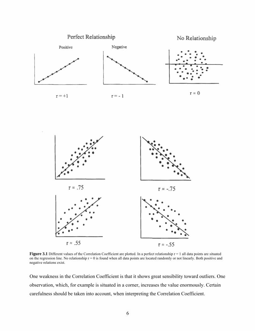
Figure 3.1 Different values of the Correlation Coefficient are plotted. In a perfect relationship r = 1 all data points are situated on the regression line. No relationship r = 0 is found when all data points are located randomly or not linearly. Both positive and negative relations exist.

One weakness in the Correlation Coefficient is that it shows great sensibility toward outliers. One

observation, which, for example is situated in a corner, increases the value enormously. Certain

carefulness should be taken into account, when interpreting the Correlation Coefficient.

6

A numerical high value on r, can be explained by: yx → Variable x influence variable y. yx ← Variable y influence variable x. yx ⇔ Mutual influence between the variables.

yzx →← One or several variables Z influence simultaneously the variables x and y without

their need of a logical connection.

It is because of the fourth point there is a reason for a careful interpretation. There are several

examples of so called nonsense correlation, where a high correlation is noticed, but without a

direct connection between the variables i.e. the Correlation Coefficient does not say anything

about causality.

3.1.3 The Significance

How significant is the correlation?

The Determination Coefficient R2 is a measurement of how well the adaptation is connected to

the y-observations. R2 is defined accordingly where yi is one data value of the time series y, is

the corresponding point on the regression line,

y

y is the mean of all yi.

∑∑

−

−−= 2

22

)()ˆ(

1yyyy

Ri

ii

Consider the numerator and the denominator; if they are the same size, the model can not explain

anything of the variables in y. If the residuals are found to be 0, the model explains all of the

variation in y. Often we get a value of r that lies somewhere in between 0 and 1 and it is

interesting to calculate R2 to see how much of the variation in y that can be explained by the

model.

7

3.2 MR Physics A strong, static, homogenous magnetic field is the foundation for all MRI. Magnetic field

homogeneity is of importance to record good quality MR images. The magnetic field in our MR

scanner is 1.5 T. The hydrogen atom is the most commonly depicted atom, since it is the most

frequently occurring atom in the human body. The proton has a spin, as a consequence of thermal

energy. The higher the temperature, the faster the movement of the proton, at the absolute zero

the protons stands still (if this is not familiar, you might reread laws of particle physics). The

proton has a positive charge and the spin movement generates electricity which generates a

magnetic momentum, when it is placed in a magnetic field. Because the magnetic momentum is

odd (in the case of hydrogen=1) the spin also results in an angular momentum. To be able to use

an atom for MRI purposes, the atom needs both a magnetic and an angular momentum. Every

odd atom number has this quality.

Without an additional magnetic field the atom-spin is oriented randomly with a very small or

non-existent net magnetism. The atoms have a spin around their own axis, which are either

parallel or anti-parallel with the magnetic field. If a strong magnetic field is added, the net

magnetism will increase. The parallel condition has a lower energy level than the anti-parallel

condition, which results in a high frequency of parallel spin. If energy is provided at a special

frequency, the so called resonance frequency or Larmor frequency, which equals the rotation rate

of the net magnetization, some spin will absorb the energy and switch to the higher energy state.

When the external energy supply is cut again, the spin will return to the lower energy state and

then emit energy in the form of a RF pulse. The Larmor frequency v is proportional to the

magnetic field B where the constant depend on the magnetic moment μ and Planck’s constant h:

v = (2μ/h) B

A birdcage head coil is used that both transmit and receive RF pulses. The coil transmits a radio

impulse of Larmor frequency that excites the protons. The spins are tipped to the transverse plan

hence changing the net magnetism:

t∂∂

−=φε

8

Yet, to acquire an image and not just a signal, introducing an additional varying magnetic field is

necessary that forces the resonance frequency of the protons at different locations to vary in

space. The idea of spatial magnetic field gradients came from the scientist Paul Lauterbur who

made it clear that measuring the emitted energy at different frequencies would encode spatial

properties of the sample being scanned. Lauterbur concluded that several gradients were needed

in order to achieve information from more than one spatial dimension. To get the full description

of the proton, 3 gradients are needed in the x, y, and z directions. Gradients to achieve a spatial

encoding are used in all MR. Nevertheless since fMRI measures vascular changes the procedure

must be rapid. The technique used is known as Echo-Planar Imaging, EPI, developed by Peter

Mansfield. Gradients are introduced quickly in a fixed manner and the emitted pulse from the

protons is picked up by the birdcage coil as an echo. Frequencies from the whole slice are

recorded at the same time. Subsequently, a Fourier transform is used to convert the frequency

data into spatial information.

The MR signal is completely gone in the range of a few seconds after the excitation pulse is taken

away. This process of extinction of the received MR signal in the coil can be described by two

time constants, T1 and T2. This depends on the spin’s gradual going back to the lower energy

condition. The return to the lower energy condition is called Longitudinal Relaxation, and the

time constant is indicated by T1. In addition to longitudinal relaxation, the spin coherence also

disappears, which is called Transverse Relaxation and the indication for this is T2. There are two

causes for transverse relaxation, one intrinsic and the other extrinsic. The intrinsic cause is from

spin-spin interaction, i.e. the many spins interact on each other. Also accounting to the loss of

coherence is that the external static magnetic field is inhomogeneous due to air-tissue

susceptibilities, presence of iron, imperfections in the scanner etc. The combined effects of spin-

spin interaction and field inhomogenity lead to a signal loss known as T2* decay which is

characterized by the time constant T2*.

3.2.1 BOLD Contrast

FMRI stands for Functional Magnetic Resonance Imaging. Functional MRI is based on the

hemodynamic response in the area of neuronal activity and uses the magnetic properties of the

haemoglobin molecule, which varies depending on the oxygen presence. De-oxygenated

9

haemoglobin is paramagnetic and disturbs the signal by creating distortions and inhomogeneities

in the magnetic field. The increase in neuronal activity of one part of the brain results in that the

brain overcompensates with an increase in blood flow (that is 2-3 times higher than required) in

comparison to the relative increase in oxygen consumption so that the net result is a decrease in

the absolute concentration of de-oxy haemoglobin, resulting in a signal increase in T2*-weighted

MR images. The phenomenon is called BOLD contrast and the mechanism is illustrated in figure

3.2.1. After a while the demand of oxygen will arise and the positive signal response attenuates

and eventually become undershoot which slowly increases to baseline. The undershoot is

probably caused by a temporal mismatch of increases in CBF and CBV and the main reason for

the positive BOLD signal returning to baseline levels is simply a return to baseline levels in

neuronal activity. Figure 3.2.2 shows the course of events in a model of BOLD response created

in Matlab, the BOLD signal has a peak after a few seconds, thereafter undershoot and then the

signal increases to baseline.

10

Brain activity

Increase in T2*

Increase in MR signal

Increase in blood flow and oxygen utilization

Oxy haemoglobin + De-oxy haemoglobin –

Decrease in magnetic susceptibility

Figure 3.2.1 The BOLD fMRI. Activity in the brain leads to increases in blood flow and oxygen utilization, which in turn leads to a local increase in oxy haemoglobin and a decrease in de-oxy haemoglobin. Since de-oxy haemoglobin is paramagnetic and disturbs the magnetic field the decrease in de-oxy haemoglobin leads to reduced magnetic susceptibility and enhanced contrast (called T2*) and MR signal.

11

Figure 3.2.2 Model of BOLD response due to finger button press. One sees the peak, undershoot and the growing back to baseline.

3.2.2 MR Contrasts and Pulse Sequences

To understand the mechanisms behind MRI, a description of the tissue contrasts and parameters

that affect the appearance of the images is needed. What is a contrast? A contrast is the difference

in the signal between any two tissues. As soon as a difference in the signal strength between two

tissues occurs, there is a contrast. It is easy to realise that if the tissues have the same signal, the

image is going to be constant, and no details appears. There are two factors that govern the time

at which MR images are collected. These two are the repetition time and the echo time and can be

manipulated to achieve a contrast in the image. The repetition time (TR) is the time interval

between the excitation pulses. The echo time (TE) is the time interval between excitation pulse

and data acquisition. Given the magnetization M0, the time constants T1 and T2, the obtained MR

signal from the equation is:

12

21 //0 )1()( TTETTR eeMtM −−−=

By choosing different T1 and T2 one is able to achieve images which are sensitive to a specific

characteristic.

T1 contrast

The most common structural contrast for anatomical images is T1 weighting. If TR is too short,

the longitudinal relaxation will not have time to recover and no MR signal is recorded. On the

other hand, if TR is too long, then all longitudinal relaxation is recovered. The meaning of these

two cases is that the amount of magnetization will be similar to both of two tissues and no

contrast is achieved. If a “middle TR” is obtained, one will receive a contrast, since there will

appear a signal difference between the tissues. This is a typical optimization problem: There is an

optimal TR to any two tissues who differs in T1. To receive an exclusive T1 contrast, we must

have very short TE to minimize T2 contrast. Summing up, a short TE and an intermediate TR is

needed to generate T1 sensitive images.

T2 contrast

Signal loss depends upon the time between excitation and data acquisition, echo time (TE). The

optimization problem: Choose TR and TE for maximizing the T2 contrast. The right choice is an

intermediate TE. Exclusive T2 contrast is obtained if the TR is very long so that the influence of

the T1 contrast vanishes.

T2* weighted images are sensitive to the amount of de-oxygenated haemoglobin present which

changes according to the metabolic demands of active neurons. T2* contrast is like T2 provided

by pulse sequences with a long TR and a medium TE. But some additional requirements are

needed which I will not discuss further here. However T2* weighted images are used in fMRI and

it is worth knowing about the conceptions of these contrasts. For the first task suitable fMRI data

already existed and for the second task all contrast parameters were already adjusted so I could

start scanning without considering them.

13

3.3 The Signal-to-Noise Ratio, SNR The signal-to-noise ratio (SNR) is one of the important measures of the performance in a MRI

system. Noise in MR images shows an overall grainy appearance in the image. During MRI

studies the magnitude of a current in the detector coil is measured, this quantity is both noise and

signal. The signal arises from changes in magnetization, e.g. the MR signal. The noise consists of

everything that is uninteresting for us to measure. There exist several kinds of noises, such as

thermal noise, system noise, scanner drift, motion artefacts and physiological noise.

Raw signal-to-noise ratio is calculated through dividing the intensity of the image in a region that

contains the sample by the intensity of the image in a region that is outside the sample. You

simply make a division of the brain signal with the signal outside the brain. As you would expect,

one is also interested in the differences in MR signal within different regions of the brain. This is

called contrast-to-noise ratio, CNR. However in this study, like in most fMRI experiments, we

want to distinguish between two states of the brain by comparing signal from a goal directed task

and a control state (resting state). Functional SNR depends upon signal intensity difference

between groups of voxels, region over time or even within a voxel. For simplicity I will refer

functional signal-to-noise ratio as signal-to-noise ratio [6].

14

4. METHOD 4.1 Introduction to SPM Different brain activations as a result of external stimuli is being analysed and measured. For

example, after a right handed button press it is possible to see a typical activation in the Left

Motor Cortex, LMC.

SPM stands for Statistic Parametrical Mapping [8]. It is a toolbox for Matlab, which calculates

the probability of the activation in every individual voxel of the brain, i.e., labelling all voxels

within the image according to the outcome of a statistical test. The goal of the statistical test is to

evaluate the probability that each voxel is consistent with the null hypothesis. When statistical

tests from all voxels in the brain are combined, the result is a statistical map or a statistical

parametric map of brain activity. The statistical results can be displayed in different ways. The

easiest way is the “Glass-brain view”, where only the activations are visible and is frequently

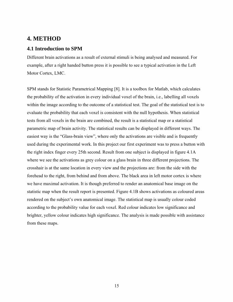
used during the experimental work. In this project our first experiment was to press a button with

the right index finger every 25th second. Result from one subject is displayed in figure 4.1A

where we see the activations as grey colour on a glass brain in three different projections. The

crosshair is at the same location in every view and the projections are: from the side with the

forehead to the right, from behind and from above. The black area in left motor cortex is where

we have maximal activation. It is though preferred to render an anatomical base image on the

statistic map when the result report is presented. Figure 4.1B shows activations as coloured areas

rendered on the subject’s own anatomical image. The statistical map is usually colour coded

according to the probability value for each voxel. Red colour indicates low significance and

brighter, yellow colour indicates high significance. The analysis is made possible with assistance

from these maps.

15

(A) (B)

Figure 4.1 Outcome of a right handed finger button press experiment. (A) Glass-brain views of the fMRI data displaying where

we got activations. The black spot shows our maximum. (B) Colour coded maps rendered on anatomical image. SPM shows three

projections and the arrow or cross hair is at same location in each brain view. In the upper left view the forehead is to the right and

we see activations from the side. The right view is seen from behind. The lower left image is taken from above with the forehead

to the right.

4.2 Pre-processing Data Raw data must be worked up before the analysis. First, the files of DICOM format are converted

so that the SPM can read them. In these experiments, 8700 files per subject are being converted

and results in 300 volumes, each containing 29 slices1. Thereafter spatial processing is carried

out.

4.2.1 Spatial Pre-processing

MRI is sensible for movements because the images are acquired at absolute spatial locations. If

the head moves, the image will be acquired with the brain in the wrong location. Motions are due

to the fact that a subject may shift the position of his/her head or swallow more, because of

nervousness. There are also small regular oscillatory motions due from regularly oscillations of

1 The DICOM Conversion was made in SPM2, while the remaining parts of the analysis were made in the later version, SPM5.

16

the heart and lungs. Despite different innovative attempts to minimize movements during the MR

scanning session, pre-processing of data is necessary for removing deviations. The deviations are

often small, about the size of a few millimetres, but in the worst of cases the movements are so

large that they may render the data completely un-interpretable. If the subject move 5 millimetres

each voxel’s time series will contain data from two different brain regions that are 5 millimetres

apart. SPM corrects for small deviations with its function Realign, which makes a least square

approximation of all the images. The meaning of Realign is to match the images spatially in time

by laying the images on top of each other and then calculate the mean. Thereafter a co-

registration is made to be able to compare a structural image with a functional image since we are

interested in how activity map onto anatomy. Functional images have typically low resolution

and little anatomical contrast whereas structural images have high resolution, are detailed and

have distinct boundaries between different tissues. Co-registration makes two different kinds of

images, like T1- and T2 weighted, resemble each other in space. For this purpose the Realign

Mean Image is used as a template (sometimes called target image) that remain stationary while

the structural image is moved to suit like a hand in glove for the template image.

A Standardisation procedure normalizes the images to a standard volume, which is defined by

some kind of ideal model or the patient’s own anatomical image. All brains do not look the same

but they are unique like our faces and differ in size, shape and anatomy. To be able to analyse

data from different subjects a normalisation is made so that the researcher can derive data from

homologous parts of the brain. Thereafter a function called Smooth is used in SPM to flatten out

the activations and quell noises and other disturbances. For this task, a Gaussian filter is used. I

used a Gaussian filter with a FWHM (Full width at half Maximum) of 8 millimetres. Without

smooth there would have been sharp delimitations between the activations but with the use from

a Gaussian kernel it is possible to achieve a more smoothed-out divide of the activity, which is

also in better accordance with reality. Smooth increases the SNR and since the activation is

spread over a range of voxels, it facilitate studies between subjects because the probability that

activation in one single voxel will agree between subjects is rare, more feasible is that the

activation appears somewhere in the adjacent area. After these steps of the pre-processing, the

data is ready for usage in models where we aim to investigate if the data we have recorded fits

hypothesises we have embodied in our model.

17

4.3 General Linear Model A statistical analysis of fMRI data is first happening through the creation of a linear model, called

regression analysis:

exbxbxbay kk +++++= ...2211

The general linear model is an equation that express the observed response variable y in terms of

a linear combination of explanatory variables x plus an error term e. The general model assumes

that the errors are independent and identically distributed with zero mean and variance σ2,

N (0, σ2) but this is not really the case in fMRI since the data at different time points correlates

with each other, so called autocorrelation [5]. Fortunately SPM take this into account by

modelling the autocorrelation with an AR(1) filter. The parameter weights bi indicates how much

each explanatory variable contributes to the overall fit of the data. The parameter a reflects the

total contribution of all variables that are held constant throughout the experiment i.e. the mean

signal interest, that we often do not concern ourselves with. A curve with a minimal deviation

from all data points is desired. The Method of Least Squares can obtain this best-fitting curve.

The vertical deviations between the searched line and the points in a spreading diagram are called

residuals. The square of the residuals shall be minimized. Explanation:

22 )()ˆ( iiii bxayyy −−=− ∑∑

The minimization is done with a partial derivation and the parameter weights are obtained after

the calculations.

The fMRI paradigms can be either event related or block designed. What determinate this is the

length of stimuli. Here we look at event related responses. This means that a stimulus lasts during

a rather short time and is illustrated graphically as a peak on a time diagram and is

mathematically described with a delta function but convoluted with a canonical hemodynamic

response function in SPM. A block design on the other hand is illustrated as boxes in the time

diagram.

18

4.3.1 The t-test

As mentioned before a statistical map is created with use from a statistical test, e.g. the t-test. The

t-test evaluates if voxels have different mean signal levels in two experimental conditions.

The t-distribution describes the expected difference between two random samples. Mean of t-

distribution is zero, since the two samples should on average have the same mean value, and the

standard deviation of the t-distribution is the sampled standard deviation divided by the square

root of the sample size.

The t-distribution has approximately the same look as a normal distribution with a mean of 0 and

a standard deviation of 1, although the t-distribution is a bit wider. The numbers of degrees of

freedom decides exactly how the t-distribution looks like. The more numbers of degrees of

freedom, the closer the t-distribution will approach to a normal distribution. The number of

degrees of freedom is often equal to the number of observations minus 1. In figure 4.3 we see a t-

distribution with 8 degrees of freedom. The t-statistic is equal to 2.30 and you can calculate (or

look up in a table) to verify that this gives an alpha value of 0.025(the black painted area).

Figure 4.3 T-distribution with 8 degrees of freedom and an alpha value of 0.025

19

A t-test is appropriate when the research question can be answered by evaluating whether or not

two samples have statistically different means. My paradigm consists of two conditions, finger

presses and rest. The null hypothesis is that there is no event-related signal evoked.

To conduct the t-test: calculate the mean from all data points during rest and calculate the mean

from all data from finger presses, then divide the difference between the two conditions by the

shared standard deviation δ. The t-statistic should be compared to the experiments Alpha value

for deciding the significance of an explanatory variable at a given voxel.

However since fMRI data contains thousands of voxels there will be thousands of t-tests

performed and the chance of a false-positive result is enhanced due to the multiple comparisons.

A solution is Bonferroni correction in which the alpha value is decreased proportionally to the

number of statistical test. If n is the number of performed t-tests, the probability for having no

false-positive results is:

n

nalphap )1( −=

But given about 40 000 voxels, n becomes very large resulting in a small value of p that is too

conservative. SPM’s solution is the random Gaussian field approach [5].

20

5. RESULT 5.1 Correction for spontaneous fluctuations

5.1.1 Model for the "Button press" paradigm

At the present fMRI study, two conditions were used. One condition defines rest and the other

defines work. For resting measurements, a rather passive, simpler task is done for making the

definition of the baseline or control state through which activity from the work paradigm can be

compared. In this experiment, the subject where shown a counter that counted from ‘1’ up to

‘24’, and when the figure ‘25’ was supposed to be shown, a red cross appeared and the subjects

where instructed to press a key with their right index finger. Thereafter the procedure was

repeated. The whole test took 600 seconds, and the last cross was shown at 599 seconds. The first

task was to describe the paradigm with a linear model. I modelled this train of key presses as a

vector of onsets of responses in Matlab. The cross symbols appeared at 24, 49….599. Thereafter

the duration and the conditions are stated. The duration is stated as 0 since it is event design and

convolved with the canonical hemodynamic response function.

A global maximum is shown in left motor cortex at certain coordinates (i.e. a cluster of activated

pixels) on the statistical map. This is exactly what we saw in figure 4.1 above. MarsBar (SPM

toolbox) is used to define a region of interest (ROI) for these coordinates. The time series data

from this ROI was extracted using an add-on toolbox (MarsBar) in SPM. It is important to

threshold high enough not to receive too many false positive activations and extensive clusters. I

threshold at p < 0.05 corrected for multiple comparisons that satisfy a T-value = 4.97. This time

series, press_lmc, is compensated for the global signal and the result sees in figure 5.1.1A. With

the use of Matlab, all the 23 button press responses were plotted together as a time-locked

average, figure 5.1.1B.

5.1.2 Model for the "Rest" paradigm

In the second experiment the subject is simply asked to relax and watch a cross, “rest”. The ROI

from the previous button press data is used and rest data is applied, which gives a new time

series, figure 5.1.2A. This time series will approximately represent the signal intensity timecourse

21

in left motor/somatosensory cortex during rest. After compensation for the global signal, the time

series will be the regressor in a new model applied on rest data. A functional

connectivity/temporal correlation between left and right cortex appears on the rest model map

shown in figure 5.1.2B. In the left motor cortex a maximal activation and correlation is seen,

which is natural, since it correlates itself. Interestingly, we now see a strong correlation in the

right motor cortex.

The task is now to define a new ROI in the right motor cortex on the basis of the rest model. Here

I threshold lower. I decided it suitable to threshold at p < 0.00005 corrected for multiple

comparisons that satisfy a T-value = 6.44. Then extract rest data to the right motor cortex ROI

and extract new time series and compensate for the global signal.

22

Figure 5.1.1 (A) Time series from button press data in LMC. (B) Time-locked average of the time series displayed in (A).

23

(A)

(B)

Figure 5.1.2 (A) fMRI time series from rest data applied on ROI in LMC. (B) Functional connectivity is seen as bright spots in left- and right MC, here displayed on anatomic base image.

24

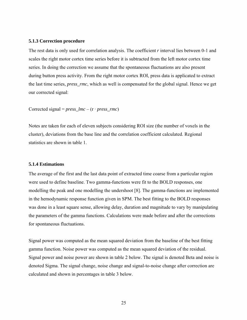
5.1.3 Correction procedure

The rest data is only used for correlation analysis. The coefficient r interval lies between 0-1 and

scales the right motor cortex time series before it is subtracted from the left motor cortex time

series. In doing the correction we assume that the spontaneous fluctuations are also present

during button press activity. From the right motor cortex ROI, press data is applicated to extract

the last time series, press_rmc, which as well is compensated for the global signal. Hence we get

our corrected signal:

Corrected signal = press_lmc – (r · press_rmc)

Notes are taken for each of eleven subjects considering ROI size (the number of voxels in the

cluster), deviations from the base line and the correlation coefficient calculated. Regional

statistics are shown in table 1.

5.1.4 Estimations

The average of the first and the last data point of extracted time coarse from a particular region

were used to define baseline. Two gamma-functions were fit to the BOLD responses, one

modelling the peak and one modelling the undershoot [8]. The gamma-functions are implemented

in the hemodynamic response function given in SPM. The best fitting to the BOLD responses

was done in a least square sense, allowing delay, duration and magnitude to vary by manipulating

the parameters of the gamma functions. Calculations were made before and after the corrections

for spontaneous fluctuations.

Signal power was computed as the mean squared deviation from the baseline of the best fitting

gamma function. Noise power was computed as the mean squared deviation of the residual.

Signal power and noise power are shown in table 2 below. The signal is denoted Beta and noise is

denoted Sigma. The signal change, noise change and signal-to-noise change after correction are

calculated and shown in percentages in table 3 below.

25

5.1.5 Results

In the plot (figure 5.1.5A) showing the uncorrected time-locked averaged BOLD responses in the

left MC, a rather clear button press response is visible but also a remarkable trial-to-trial

variability. Consider figure 5.1.5 where both uncorrected and corrected button press responses are

exposed.

A

26

B

Figure 5.1.5 Bold Responses from 23 finger button presses, before (A) and after (B) the subtraction of spontaneous fluctuations

in right motor cortex of one Subject.

Generally the signal is weakened a bit (mean value = -14%) and the noise is decreased with

approximately 30 %. In table 3 one sees that noise decreases in all the subjects after correcting

for spontaneous fluctuations. Obvious noise reduction is compensated by a weakened MR signal.

The noise reduction though is bigger than the weakening of the signal. It is interesting to

calculate and distinguish the change in the signal-to-noise ratio before and after the correction.

We observe that in six out of eight subjects, the signal -to- noise is far improved after the

correction. In subject number 10 as much as 112%! Although two subjects shows a worsening in

the signal-to-noise ratio. Three subjects diverge far from the other in that they does not show

activated voxels in right motor cortex, one of them did not even show activated voxels in the

brain at all. I tried to clear this up by choosing higher alpha values maybe I was too strict? But

no, the glass-brain view still appeared empty.

27

Table 1 The coordinates (x,y,z), ROI sizes (number of voxels) and correlation coefficient for each subject.

Left motor cortex region Right motor cortex region Subject Coordinates Size (voxels) Coordinates Size (voxels) Correlation coef 5 -44 -48 64 1019 58 -38 52 515 0.37 6 -36 -40 66 809 42 -40 60 1073 0.54 8 -34 -34 72 1220 48 -40 58 515 0.63 10 -46 -20 60 841 28 -40 62 940 0.91 11 -34 -26 68 269 showed no activity in right motor cortex 12 -38 -44 66 280 58 -34 30 239 0.50 13 showed no activity in motor cortex 15 -54 -58 44 200 showed no activity in right motor cortex 16 -36 -46 68 157 36 -20 72 287 0.50 17 -30 -26 72 2187 44 -18 66 510 0.83 18 -52 -28 46 1507 60 -20 40 1545 0.83 Table 2 Signal power (Beta) and noise power (Sigma) before and after the correction for intrinsic activity. Subject Beta before Sigma before Beta after Sigma after 5 11.1451 3.4571 9.2349 3.2047 6 7.3801 2.8761 6.0870 1.8934 8 8.5033 2.0273 6.6616 1.3330 10 7.4660 2.3435 9.8737 1.4567 12 9.5866 9.0989 7.5822 8.7522 15 7.4073 7.1396 16 6.9556 7.4565 7.5652 5.7657 17 8.9752 1.8742 5.4783 0.6046 18 7.0350 2.2168 4.6886 1.3014

28

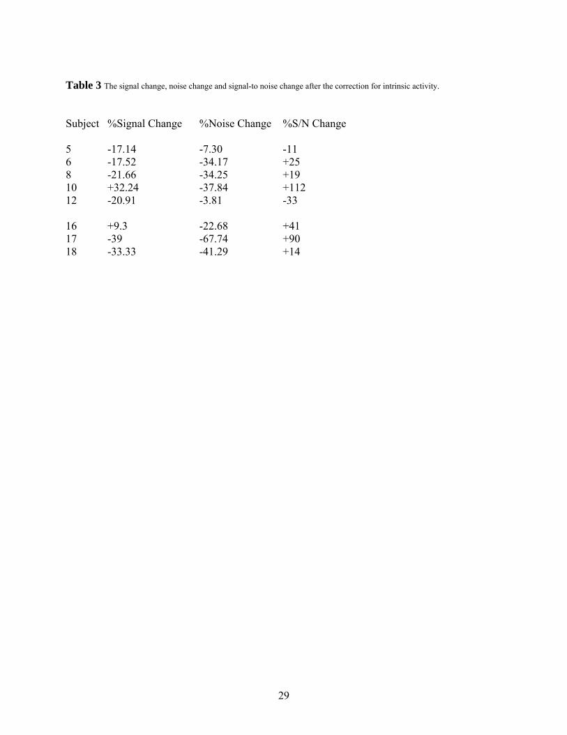
Table 3 The signal change, noise change and signal-to noise change after the correction for intrinsic activity.

Subject %Signal Change %Noise Change %S/N Change 5 -17.14 -7.30 -11 6 -17.52 -34.17 +25 8 -21.66 -34.25 +19 10 +32.24 -37.84 +112 12 -20.91 -3.81 -33 16 +9.3 -22.68 +41 17 -39 -67.74 +90 18 -33.33 -41.29 +14

29

5.1.6 Conclusion

We see in table 1 that the size of the ROI varies between the subjects. This depends on the voxel

activation, which is highly individual, some people get many activated voxels and others get few.

Individual deviations are one explanation to differences in result. Another example of individual

deviation is the global maximum, which is situated on different coordinates on all individuals.

The fact that the results differ could also depend on the scanner, or that the subject is counting or

rehearsing during the control state. On the basis of the results we see that it is possible to reduce

the trial-to-trial variability of the MR signal through calculating the intrinsic activities and then

subtract it from the total activity, which is measured.

30

5.2 Reaction times and intrinsic activity

5.2.1 Collection of new data

In the second part of this Master Thesis I wanted to evaluate whether intrinsic signal fluctuations

might affect reaction times. This required a new collection of data. Since it is a pilot study, it is

enough to examine only one subject, to see if it is possible to find any relations to build further

upon.

Since I did not know the paradigm details in advance, I could be the subject myself. Each

paradigm was 600 s long and when a blue circle turned into a red cross, the instruction was to

press the button as fast as possible with the right index. The purpose was to minimize the reaction

time as much as possible each time, a bit like a competition with myself to receive the fastest

result. It was important to keep the motivation up during the whole paradigm length. I did not

know in advance which times the cross would show on the screen, the crosses had been put in at

different times, some crosses came up close after one another, and some crosses took longer time

to appear. The reason for this was to make it hard for me to guess when the next cross was going

to appear, and therefore eliminate this source of error and upholding credibility. Only the button

presses that are 20 s apart can be used. This is because of the avoidance of unlinearities in the

hemodynamic BOLD response that can come up if the responses are overlapping each other.

Data was collected from 3 such paradigms. After this process, a series of anatomical images were

taken, one shorter session with 152 scans, and one rest paradigm. The rest paradigm task was just

to lay down, relaxing and look at the cross.

5.2.2 Method for analysing new data

After the pre-processing of data, which was made in a customary way as described above, the

next step was to sort out the times which had the button presses 20 s apart. There were 19 in each

session (in total 3*19). For each event, I extracted a BOLD response and saved those in a vector

for later usage. The shorter session was used alone to define the Region of Interests (ROI) in the

left motor cortex. I connected rest data to this ROI to be able to put it in as an independent

regressor in the next model to apply rest data upon, and to find a suitable ROI in the right motor

31

cortex. Both ROIs were created as 10 mm spheres, centred on the relevant coordinates. It was

suitable to get a rather big proportion of coherence between the activated voxels. The coordinates

and sizes of the ROIs are presented in table 4.1. So far the steps were the same as in the first part.

But thereafter it was time to apply new data to the ROI in the right motor cortex and extract the

time series from these. Data was thus connected from the first session to the cluster, and from the

cluster the time series was picked out. The global signal was erased as well as the mean. The

same was done with sessions 2 and 3. A preliminary analysis of the time series and the response

times was made to begin with. I draw a plot to see if I could discover any connections with the

plane eye on the basis of the spreading diagram.

A Band-pass filter was added to the time series to remove the drift in the signal. Otherwise there

is a risk for obtaining an incorrect result, because the time series might drift with time. I plotted x

and y, where x is the vector of all fixed time series from the right motor cortex and y is the

measured response time. A weak tendency is discovered. At the peak in the bold response there

are longer response times, but when there is a decrease in the bold response, the response times

are shorter.

I calculated the correlation coefficient between x and y. I tested some different points in time

during the calculation, exactly at the onset time, 1-4 s after and 1-4 s before to find out at what

time there was the highest correlation. The correlations coefficients are listed in table 4.2.

Summary of the Methods:

1) Extract the time series from the RMC cluster

2) Compensate for a global signal, subtract the mean and Band-pass filter

3) Pick out only the responses which are 20 s apart

4) Pick out the belonging relevant onset times

5) Pick out the values of the time series at the onset times and mark the corresponding response

times, plot

6) Calculate the correlation coefficient between the response times and the time series values

around the onset time. Examine at which time there is the highest correlation

7) Plot all the 3 sessions in the same diagram.

32

5.2.3 Results and discussion

When reflecting on figure 5.2.1, a weak but persistent tendency is noticed. The correlation

coefficient is 0.3412 and significant**. The R2 is 0.8836, which means that more than 88% of the

connection is explained by the regression coefficient. It is therefore possible to draw the

conclusion that the reaction times are dependent on the amplitude of the spontaneous

fluctuations, the higher the value of the bold response, the longer reaction time. A low value on

the spontaneous activity affects the reaction time in a positive manner so it becomes shorter.

Figure 5.2.1 Plot of data from the three sessions. There is a weak but persistent correlation between the amplitude of the bold response and the time response.

I still want to encourage being careful when interpreting the result above. We have only analysed

data from one subject, with the knowledge that there occur enormous individual deviations we

can not be completely sure that the result is not a discrepancy from the norm. Maybe a study of

20 subjects would have given an opposite result. Although, what makes this a credible result is

33

because the activation of the brain voxels looked like expected with a maximum activation in the

left motor cortex. The three sessions also follows the same pattern with a correlation of > 0.3 as

you may verify from the correlation plots shown below. Figure 5.2.2 shows the result from the

first session, figure 5.2.3 shows the result from the second session and figure 5.2.4 shows the

result from the third session.

Figure 5.2.2 The result from first session. The rings mark the button finger presses.

34

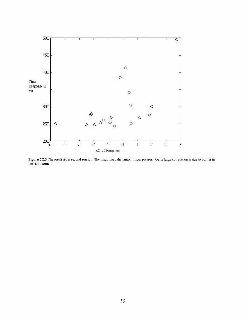
Figure 5.2.3 The result from second session. The rings mark the button finger presses. Quite large correlation is due to outlier in the right corner.

35

Figure 5.2.4 The result from third session. The rings mark the button finger presses.

Table 4.1 Coordinates and size of ROI.

Left Motor Cortex Right Motor Cortex

Coordinates Size (voxels) Coordinates Size (voxels)

-50 -38 60 515 58 -38 54 515

Table 4.2 The estimated correlation coefficient for each session.

Session Correlation Coefficient

Session 1 0.40

Session 2 0.60

Session 3 0.40

Session 1, 2, 3 0.34

36

5.2.4 Conclusion

There seems to be a connection between behavior and intrinsic spontaneous fluctuations. The

spontaneous fluctuations are nothing we can steer and it is easy to draw the conclusion that the

reaction times are not completely under our will either. Other factors that we know affect the

result are the level of tiredness, motivation, and the general condition of the subject. I have tried

to aim at the shortest reaction times possible in my study; I have been competing against myself

and tried to keep my motivation on top to minimize the response times. This single experiment

shows promising results regarding the hypothesis that intrinsic brain activity influence response

times. But the results is based upon only one subject and much further work is needed in order to

fully understand this issue and with certainty conclude that the suggested relationship exist. The

results above are very preliminary and reflect work in progress.

37

6. CONCLUSIONS Intrinsic activity is low frequent fluctuations occurring spontaneously in the resting brain. We can

assume that these fluctuations are present even during work and by accounting for them the noise

is reduced and the signal-to-noise ratio is approved. A relation between intrinsic activity and

behaviour is likely to exist. My pilot study shows promising results regarding that intrinsic

activity influence reaction times. Larger BOLD amplitudes of the intrinsic activity seem to cause

longer reaction times but this assumption might fail due to for instance individual deviations.

38

7. FUTURE WORK To conclude whether reaction times are influenced by the intrinsic activity much further work is

required in order to fully understand this issue. Appropriate future work is to try to reproduce my

study on several healthy subjects and readdress if the suggested relationship exists. How intrinsic

activity affects human behaviour is fairly unexplored and there lies further work in more

research.

39

Acronyms

BOLD Blood Oxygen Level Dependent CBF - Cerebral Blood Flow CBV - Cerebral Blood Volume EPI - Echo-Planar Imaging fMRI - functional Magnetic Resonance Imaging LMC - Left Motor Cortex MC - Motor Cortex RF - Radio Frequency RMC - Right Motor Cortex ROI - Region Of Interest SNR - Signal-to-Noise Ratio

40

Bibliography

[1] Bharat Biswal, F. Zerrin Yetkin, Victor M. Haughton, James S. Hyde. Functional Connectivity in the Motor Cortex of Resting Human Brain Using Echo-Planar MRI. MRM 34:537-541, 1995 [2] Michael D Fox, Abraham Z. Snyder, Jeffrey M Zacks, Marcus E Raichle. Coherent spontaneous activity accounts for trial-to-trial variability in human evoked brain responses. Nature Neuroscience, published online 2005-12-11 [3] Göran Andersson, Ulf Jorner, Anders Ågren. Regressions- och tidsserieanalys. Studentlitteratur. Lund. 1994 [4] Gunnar Blom. Sannolikhetsteori och statistikteori med tillämpningar. Studentlitteratur. Lund.1989 [5] R.S.J Frackowiak, K J Friston, C.D Frith, R.J Dolan, J.C Mazziotta. Human Brain Function. Academic Press. Canada. 1997 [6] Scott A. Huettel, Allen W. Song, Gregory McCarthy. Functional Magnetic Resonance Imaging. Sinauer Associates, Inc. 2004 [7] Bryan Kolb, Ian Q. Whishaw. Human Neurophysiology. W.H. Freeman and Company. New York. 1996 [8] http://www.fil.ion.ucl.ac.uk/spm/. Last visited 2006-11-22

41

TRITA-CSC-E 2007:005 ISRN-KTH/CSC/E--07/005--SE

ISSN-1653-5715

www.kth.se