investigation of the sources and sinks of atmospheric methane
TRANSCRIPT

Portland State University Portland State University
PDXScholar PDXScholar
Dissertations and Theses Dissertations and Theses
2010
Investigation of the sources and sinks of Investigation of the sources and sinks of
atmospheric methane atmospheric methane
Christopher Lee Butenhoff Portland State University
Follow this and additional works at: https://pdxscholar.library.pdx.edu/open_access_etds
Part of the Chemistry Commons, and the Physics Commons
Let us know how access to this document benefits you.
Recommended Citation Recommended Citation Butenhoff, Christopher Lee, "Investigation of the sources and sinks of atmospheric methane" (2010). Dissertations and Theses. Paper 2813. https://doi.org/10.15760/etd.2807
This Dissertation is brought to you for free and open access. It has been accepted for inclusion in Dissertations and Theses by an authorized administrator of PDXScholar. Please contact us if we can make this document more accessible: [email protected].

ABSTRACT
An abstract of the dissertation of Christopher Lee Butenhoff for the Doctor of Philosophy
in Applied Physics presented June 11, 2010.
Title: Investigation of the Sources and Sinks of Atmospheric Methane
Methane (CfLi) is a potent greenhouse gas and its atmospheric abundance has .nearly
tripled since pre-industrial times. With a radiative forcing of 0.48 W m-2 it is second only
to carbon dioxide in changing the radiative balance of the atmosphere. The behavior of
CH.i has been interesting in recent years. After nearly a century of rapid growth fueled by
anthropogenic emissions from sources such as agricultural production and energy, in the
past two to three decades the trend of CRi has declined to nearly zero, and its growth
today is stalled. There is much interest in understanding why and how CRi changes on
decadal time scales, not only to explain past behavior but more importantly to predict
where CRi is heading in the future. This has implications not only for future climate
change, but also for mitigation policies that aim to reduce emissions of greenhouse gases.
The work presented here represents a number of independent studies that
investigated various components of the CHi budget, namely the sources and sinks. We
used a chemical-tracer model and created unique long-term time series of atmospheric
CRt, carbon monoxide (CO), molecular hydro$en (H2), and methylchloroform
(CH3CCh) measurements at marine background air to derive histories of atmospheric
hydroxyl radical (OH) - the main .chemical oxidant .of CRi, biomass burning - an

important source of Cl4 in the tropics, and emis~ions of CfL from rice paddies - one of
the largest anthropogenic sources of c14," over decadal scales. Globally gridded
inventories of CH4 emissions froin rice paddies and terrestrial vegetation were created by
synthesizing greenhouse and field CH4 fluxes, satellite-derived biophysical data, and
terrestrial geospatial information.
Our main finding is. that although global sources and sinks of Cf4 appear to be in
balance now, as evidenced by stable levels of atmospheric CI4, this is likely due to
competing trends in individual sources and sinks. In particular we.find good evidence that
atmospheric OH levels have declined by 10-15% over the past few decades, with most of
this change happening in the northern hemisphere. If so, this implies that glo~al Cl4
emi~sioris have f~llen by abo~t 50 Tg y-1 in the northern hemisp~ere. We find that this
decrease is due in part to declining emissions of Cf4 from rice production in China
driven by changes in agricultural practices there: In the southern tropics we find that
biomass burning emissions have risen per~aps as much as 20%, though no significant
change is observed in the northern tropics. Finally, if terrestrial vegetation is a source of
CfL, which recent reports indicate to be S?, our work shows that it is potentially
·significant globally, up to 30 Tg y-1 as constrained by the ice core record. Emissions from
this source co~ld vary significant! y on deca<;ial scales due to pressures from climate and
human activities such as land clearing and deforestation, and may balance the increase in
e~ssisons from biomass burning. A dynamic picture of CfLi emerges from this work.
The near-constant global burden of CfL seen today hides the changing behavior of the
sources and sinks beneath .. Our findings will help us understand whether Cf4 levels will
remain stable in the future.
2

Dedication
To my family ...
andTMZ.
1

ACKNOWLEDGEMENTS
As a child I never knew what a Ph.D. was or what scientists do. I only knew
they wore white lab coats and peered inquisitively into bubbling beakers of colorful
liquids (alas I do neither, which seriously calls into question whether I'm a real
scientist!). But I had good teachers. Completion of this dissertation is the cap on my
formal education that stretches back to Mrs. Beyers' morning kindergarten class at
Minnesota City Elementary School in southeastern Minnesota, and continued there in
the classrooms of Mrs. Taylor, Mrs. Fort, and Mrs. Poppe, in whose class I learned what
a googol was before it could be googled. I thank all the teachers I had at Minnesota City
and Goodview Elementary Schools, and Winona Junior and Senior High Schools. These
teachers created a solid foundation for me to pursue higher education.
A good adviser does more than just advise, and this is certainly the case for my
adviser, Aslam Khalil. Throughout my program, not only has Aslam been a guiding
influence, but he has provide me opportunities to engage in the broader scientific
community such as attending and organizing scientific conferences and meetings, and
reviewing and contributing papers to books and other publications. Aslam is a world
class scientist and I have learned much under his guidance. But beyond that I've
enjoyed our many long talks on politics, economics, human nature, religion, cycling,
and any number of other topics completely unrelated to methane. I have sincerely
enjoyed working with him and thank him for his support.
ii

I would also like to thank the other members of my dissertation committee, Erik
Bodegom (Physics), David Ervin (Economics), James Pankow (Chemistry and Civil &
Environmental Engineering), and Andrew Rice (Physics). My journey through this
program has been somewhat unorthodox and my committee members were very kind in
their understanding and flexibility
Martha Shearer has been a constant member of our research group since I
arrived. She manages all the day-to-day research activities and is the go-to person for
everything from key requests to data sources, besides being a top-notch scientists to
boot. She's invaluable to all work done in the group. Most importantly she ensures that
our Friday research meetings (typically) end at a reasonable time.
There have been a number of students and post-docs who have passed through
our group in the years I've been here, Kiren Bahm, Conrado Salas Cano, Aida Biberic,
Zhengqin Xiong, Doug Parsons, Alec Sithole, Ellyne Kutsche, and Will Porter. Their
friendship made this process much mo~e bearable.
Additional thanks to James Pankow and Martha Shearer for their meticulous
reading and editing of my dissertation .. It is significantly better as a result.
Words can't fully convey my appreciation to my parents Ed and Nora
Butenhoff. First for creating a home environment where academics and knowledge were
valued which led to my pursuit of graduate education. But more importantly for always
being there for me. My pursuit of a Ph.D. took me thousands of miles away from home,
and yet they never once questioned my path. Even at that distance they've been my
iii

biggest cheerleaders and have been a very important part of this work. A million thanks
are not enough.
Finally I wish to thank my partner in life, Teresa Zahariades. I couldn't ask for a
better person to share this experience with. She alone has felt the day-to-day trials and
tribulations of these past years most keenly and has given me nothing but
encouragement and support throughout. My everlasting thanks to her is not enough.
This degree is as much hers as mine.
iv

Investigation of the Sources and Sinks of
Atmospheric Methane
by
Christopher Lee Butenhoff
A dissertatiqn submitted in partial fulfillment of the requirements for the degree of
Doctor of Philosophy in
Applied Physics
Dissertation Committee: M. Aslam K. Khalil, Chair
Etik Bodegom David Ervin
James Pankow Andrew Rice
Portland State University ©2010

--------------------------------------------------------------------------------------i----·
'{able of Contents
Dedic.ation .......................................................................................................................... i
ACKNOWLEDGEMENTS ............................................................................................. ii
List of Tables ............................................... .' ................................................................... xi
L . fp· .. 1st o 1gures ................................................................................................................. x11
Chapter 1 - A Changing World: The Importance of Atmospheric Methane .............. 1
1.1 Introduction . . . . . . . . . . .. . . . . .. . .. . . . . . . . . . . .. . .. . . .. . . . . . . . . . . . . . . . . . . . . . . . . .. . .. . . . . . . . . . . . . .. . . . .. . . . . . . . . . . . . . . 1
1.2 Mitigation Potential .......................................................................................... 5
1.3 Structure of dissertation .................................................................................... 6
1.4 Closing thoughts ...................................... ···········~.·!······ ..................................... 7
Chapter 2 - Inverse Modeling of Atmospheric Methane Mixing Ratios .................... 9
2.1 Introduction ...................................................................................................... 9
2.2 Composite CH4 record ................................ :·········································· .. ······· 10
2.3 Trend of the composite record ........................................................................ 16
2.4 Inverted sources.............................................................................................. 19
2.5 Discussion ....................................................................................................... 23
Chapter 3 - Is The Chemical Oxidation Sink Of Methane Changing? ................... 25
3 .1 Introduction .................................................................................................... 25
3.2 Emissions ........................................................................................................ 33
v

---------------------------------------------,--:-!
3.3 Atmospheric methylchloroform measurements ............................................. 35
3.3.1 Oregon Graduate Institute ...................................................................... 35
3.3.2 ALE/GAGE/AGAGE ............................................................................. 36
3.3.3 NOAA ESRL-GMD ............................................................................... 38
3.3.4 Comparison of MCF networks ............................................................... 39
3.4 Modeling ......................................................................................................... 40
3.4.1 Description of transport model ............................................................... 40
3 .4.2 Inversion scheme .................................................................................... 44
3.4.3 Temperature ............................................................................................ 46
3.4.4 Initialization scheme ............................................................................... 48
3.5 Results ............................................................................................................ 51
3.5.1 Atmospheric lifetimes ............................................................................ 56
3.6 Sensitivity of the OH record ........................................................................... 59
3.6.1 Model and inversion method .................................................................. 59
3.6.2 Temperature trends ................................................................................. 60
3.6.3 Absolute calibration ................................................................................ 64
3.6A Emissions ................................................................................................ 67
3.7 HCFC-22 ......................................................................................................... 74
3.8 Discussion ....................................................................................................... 81
Chapter 4 - Assessment Of Biomass Burning On Decadal Scales Using
Atmospheric Measurements of Carbon Monoxide and Hydrogen ................................. 84
4.1 Introduction ..................................................................... : .............................. 84
vi

4.2 Methods of biomass burning assessment ....................................................... 85
4.2.1
4.2.2
Bottom-up methods ................................................................................ 86
Top-down method .................................................................................. 90
4.3 Time series of atmospheric CO and H2 .......................................................... 94
4.3.1
4.3.2
4.3.3
001 ......................................................................................................... 95
NOAA-GMD .......................................................................................... 98
CSIRO .................................................................................................. 101
4.3.4 Comparison of data sets ........................................................................ 110
4.3.4.1 Carbon monoxide ............................................................................. 110
4.3.4.2 Hydrogen .......................................................................................... 117
4.3.5 Composite record .................................................................................. 121
4.4 Modeling ....................................................................................................... 126
4.4.1 Sink processes ...................................................................................... 131
4.4.2 Oxidation of metliane ........................................................................... 135
4.4.3 Inversion ............................................................................................... 137
4.5 Source deconvolution· ................................................................................... 139
4.5.l
4.5.1.l
4.5.1.2
4.5.1.3
4.5.1.4
4.5.2
Sources of CO and H2 in the tropics ..................................................... 143
Direct natural sources ....................................................................... 143
Direct anthropogenic sources ........................................................... 145
Oxidation of natural NMHCs ........................................................... 146
Oxidation of anthropogenic NMHCs ............................................... 149
Emissions from biomass burning ............................ : ............................ 151
vii

4.5.3 Fire counts ............................................................................................ 159
4.5.4 Integration of source peaks ................................................................... 162
Chapter 5 - Variability Of Methane Flux From Rice Paddies ................................ 164
5.1
5.2.
5.3
5.4
5.4.1
5.4.2
5.4.3
5.4.4
5.4.5
Introduction .................................................................................................. 164
Empirical functions of spatial and temporal variability ............................... 170
Modeling Approach ...................................................................................... 176
Results .......................................................................................................... 181
Question ( 1) .. . . . . . .. . . . . . . . . . . . . . . . . . . . . . . . . . .. . . . .. . .. . . . . . .. .. . . . . . . .. .. .. .. . . .. .. . . . . . . .. . . . . . . .. . 184
Question (2) .......................................................................................... 187
Question (3) .......................................................................................... 188
Question ( 4) .......................................................................................... 188
Question (5) .... : ..................................................................................... 191
5 .5 Discussion and Conclusions ............ : ............................................................ 191
Chapter 6 - Application of an Empirical Rice Flux Model to National and Global
Spatial Scales ................................................................................................................. 193
6.1 Introduction ............................................... ; .................................................. 193
6.2 PSU-Rice Emissions Model ......................................................................... 199
6.3 Model inputs ................................................................................................. 202
6.3.1 Location and extent of rice growing areas ........................................... 204
6.3.2 Crop phenology .................................................................................... 204
6.3.3 Soil temperature .................................................................................... 205
6.3.4 Organic carbon inputs ........................................................................... 208
viii

6.3.5 Nitrogen inputs ..................................................................................... 214
6.3.6 Inundation ............................................................................................. 215
6.4 Methane fluxes and emissions ...................................................................... 218
Chapter 7 -Trends of Methane Emissions From Rice Fields and Mitigation Potential
229
7 .1 Introduction .................................................................................................. 229
7 .2 Changes in drivers ........................................................................................ 230
7 .2.1 Harvested area ...................................................................................... 231
7.2.2 Water management ............................................................................... 232
7 .2.3 Fertilization ........................................................................................... 234
7 .3 Temperature .................................................................................................. 239
.7.4 Emission trends (1961-2000) ....................................................................... 242
. 7 .5 Future trends and mitigation possibilities ..................................................... 244
7.6 Mitigation potential of rice agriculture ........................................... : ............. 247
Chapter 8 - Global Modeling Of Aerobic Methane Emissions From Terrestrial
Plants 253
8.1 Introduction .................................................................................................. 253
8.2 Previous emission estimates ......................................................................... 257
8.3 Vegetation emissions model ......................................................................... 259
8.4 Leaf biomass maps ....................................................................................... 261
8.4.1 Method 1: Leaf area index .................................................................... 261
8.4.2 Method 2: Aboveground net primary production ................................. 263
ix

8.5 Methane emissions from foliage biomass .................................................... 264
8.6 Results .......................................................................................................... 265
8. 7 Emissions from non-wetlands ...................................................................... 269
8.8 Top-down constraints on plant emissions .................................................... 270
8.8.1 Historical constraints from ice-core record .......................................... 272
Chapter 9 -Conclusion ........................................................................................... 277
9.1 Summary ....................................................................................................... 277
9.2 Closing thoughts ........................................................................................... 284
References .................................................................................................................... 286
x

Table 1.1
Table 1.2
Table 3.1
Table 3.2
Tab le 4.1
Table4.2
Table 4.3
Table 4.4
List of Tables
Radiative properties of long-lived greenhouse gases................. 2
Sources and sinks of atmospheric C~ . . . . . . . . . . . . . . . . . . . . . . . . . . . . . . . . . 4
Effective atmospheric temperatures (K) for model regions ... ... . .. 47
Inferred OH trend from c;lifferent measuring networks . . . . . . . . . . . . . .. 51
Sites and dates of CO measurements . . . . . . . . . . . . . . . . . . . . . .. . . . . . . . . . . . . 93
Sites and dates of H2 measurements ............... ·. . .. . .. . . . . . .. . . . . . . . 94
Trends of the CO composite time series . . . . . . . . . . . . . . . . . . . . . . . . . . . . . . . 125
Trends of the H2 composite time series . . . . . . . . . . . . . . . . . . . . . . . . . . . . . . . . 126
xi

List of Figures
Figure 2.1 NOAA-GMD measurements of CH4 at northern mid-latitude
sites . . . . . . . . . . . . . . . . . . . . . . . . . . . . . . . . . . . . . . . . . . . . . . . . . . . . . . . . . . . . . . . . . . . . ... 10
Figure 2.2 Ratio of CH4 measurements taken by the OGI and NOAA-GMD
networks . . . . . . . . . . . . . . . . . . . . . . . . . . . . . . . . . . . . . . . . . . . . . . . . . . . . . . . . . . . . . . . . . . 12
Figure 2.3 The composite record of atmospheric CH4 constructed by
linking the OGI and NOAA data sets................................. 13
Figure 2.4 The moving trend of the composite CH4 record . . . . . . . . . . . . . . . . . . . . . 14
Figure 2.5 The global inverted CH4 emissions modeled from the composite
data record . . . . . . . . . . . . . . . . . . . . . . . . . . . . . . . . . . . . . . . . . . . . . . . . . . . . . . . . . . . . . . . . 17
Figure 2.6 Same as in Fig. 2.5 except here emissions are for the northern
hemisphere only··················································.···.... 18
Figure 2. 7 Same as in Fig. 2.5 except here emissions are for the southern
hemisphere . . . . . . . . . . . . . . . . . . . . . . . . . . . . . . . . . . . . . . . . . . . . . . . . . . . . . . . . . . . . . . . 20
Figure 2.8 Predictions of a one-box model assuming constant emissions of
Figure 3.1
Figure 3.2
Figure 3.3
Figure 3.4
Figure 3.5
Figure 3.6
550 Tg y-1 and a lifetime of 8.9 yr . . . . . . . . . . . . . . . . . . . . .. . .. . . . . . . . .. .. 22
The effect of an OH trend over the years 1978 to 2000 on trace
gas emissions estimated using inversion techniques . . . . . . . . . . . . .. . . . 30
Emissions of methylchloroform from industrial production . . . . . . . 33
Gaps in the measurement record of OGI methylchloroform . . . . . . . 35
ESRL-GMD methylchloroform measurements from northern
mid-latitude sites . . . . . . . . . . . . . . . . . . . . . . . . . . . . . . . . . . . . . . . . . . . . . . . . . . . . . . ... 38
Ratio of AGAGE and OGI CH3CC13 mixing ratios measured at
common sites ........................................................... . 39
Methylchloroform measurements from the· OGI,
ALE/GAGE/AGAGE, and ESRL-GMD networks ................ . 44
r
xii

Figure 3.7 Simulated methylchloroform is compared with measured data
from the ALE/GAGE/AGAGE network ........................... .. 49
Figure 3.8 Derived OH using ALE/GAGE/AGAGE, ESRL-GMD, and OGI
methylchloroforrn measurements . . . . . . . . . . . . . . . . . . . . . . . . . . . . . . . . . . . . .. 53
Figure 3.9 The ratio of ESRL and AGAGE MCF at Samoa and Cape Grim 56
Figure 3.10 Stratospheric profiles of methylchloroform.. .. .. . . .. . .. . . . . . . . ... ... 57
Figure 3.11 Tropospheric temperature trends over 1979-2000.. .. . ...... .. ...... 62
Figure 3.12 Changes in simulated OH due to differences in MCF calibration. 65
Figure 3.13 Comparison of OH anomalies from the base-run and a model run
66
Figure 3.14 Comparison of model-inverted emissions and estimates of MCF
industrial emissions . . . . . . . . . . . . . . . . . . . . . . . . . . . . . . . . . . . . . . . . . . . . . . . . . . . . . 68
Figure 3.15 Addition of biomass burning CH3CC13 source to industrial
Figure 3.16
Figure 3.17
Figure 3.18
Figure 3.19
Figure 4.1
Figure 4.2
!i~ure 4.3
Figure 4.4
Figure4.5
Figure4.6
Figure4.7
emissions................................................................. 71
Anomalies of the derived OH from industrial emissions only ... .
Atmospheric concentration of HCFC-22 ........................... .
Atmospheric OH derived from HCFC-22 and MCF records ...... .
Emissions of HCFC-22 ................................................ .
Sources of H2 and CO given as percent of total budget ........... .
CO volume mixing ratios for Mauna Loa and Cape Kumukahi ... .
Seasonal cycle of CO and H2_ mixing ra~ios at Cape Kumukahi
73
76
77
79
91
96
and Mauna Loa . . . . . . . . . . . . . . . . . . . . . . . . . . . . . . . . . . . . . . . . . . . . . . . . . . . . . . . . . . 97
Volume mixing ratios of H2 measured at Mauna Loa (dashed
line) and Cape Kumukahi (solid gray) ............................... . 99
Comparison of (a) CO and (b) H2 seasonal cycles at several
NOAA-GMD northern midlatitude sites............................. 100
CSIRO-CO measurements at northern mid-latitudes............... 102
Atmospheric H2 mixing ratios from three different trace gas 105
xiii

Figure 4.8
Figure 4.9
monitoring networks ................................................... .
Atmospheric CO measurements from three different trace gas
monitoring networks . . . . . . . . . . . . . . . . . . . . . . . . . . . . . . . . . . . . . . . . . . . . . . . . . . . . 107
Latitudinal gradient.of H2 measured by three different networks.. 109
Figure 4.10 Ratios of (a) H2 and (b) CO mixing ratios measured by different
networks . . . . . . . . . . . . . . . . . . . . . . . . . . . . . . . . . . . . . . . . . . . . . . . . . . . . . . . . . . . . . . . . . . 111
Figure 4.11 Seasonal cycles of CO at different sites and measured by
Figure 4.12
Figure 4.13
Figure 4.14
Figure 4.15
Figure 4.16
Figure 4.17
different networks . .. .. . . . .. . .. . . . . .. . . . . .. . . . . . . .. .. .. . .. .. . .. . . .. . . .. ... 113
Adjusted CO records at different sites and by different sampling
networks . . . . . . . . . . . . . . . . . . . . . . . . . . . . . . . . . . . . . . . . . . . . . . . . . . . . . . . . . . . . . . . ... 115
Evidence of a calibration drift is seen in the time series of
calibration ratios . . . . . . . . . . . . . . . . . . . . . . . . . . . . . . . . . . . . . . . . . . . . . . . . . . . . . . . . . . 118
Seasonal cycles of H2 at different sites and measured by different
networks . . . . . . . . . . . . . . . . . . . . . . . . . . . . . . . . . . . . . . . . . . . . . . . . . . . . . . . . . . . . . . . . . 120
Composite time series of CO using measurements from the OGI
and NOAA-GMD networks . . . . . . . . . . . . . . . . . . . . . . . . . . . . . . . . . . . . . . . . . . 122
Analysis of CO seasonal cycles in the northern hemisphere . . . . . . 124
Composite time series of H2 using measurements from the OGI
and CSIRO networks..................................................... 128
Figure 4.18 Average seasonality of H2 soil deposition velocities for the six
latitudinal regions of our simulation . . . . . . . . . . . . . . . . . . . . . . . . . . . . . . . . . 135
Figure 4.19 CO production from C~ oxidation.................................. 137
Figure 4.20 Simulated (a) CO and (b) H2 emissions based on our inversion.. 141
Figure 4.21 Simulated emissions from inversion for the south tropical (ST)
region . . . ... . . .. . . . . .. . . . . . . . . . . . . . . . . . . . .. . . . . .. . . . . . . . . . . . . . . . . . . .. .. . . . . 142
Figure 4.22 CO emissions from anthropogenic sources........................... 145
Figure 4.23 .Emissions of (a) CO and (b) H2 from the oxidation of terpenes
and isoprene .................................. .... ......................... 149
Figure 4.24 Emissions of hydrocarbons from anthropogenic sources . . . . . . . . . .. 151
xiv

Figure 4.25 Inverted emissions with contributions from the oxidation of
natural NMHCs removed . . . . . . . . . . .. . . . . . . .. . . . . . . . . . . . . . . . . . . . . . . . . . .. 152
Figure 4.26 Deseasonalized inverted emissions of CO and H2 in the (a)
northern tropics (NT) model region, and the (b) southern tropics
(ST) regions ..... ... ... . .. .. . ... . .. .. . .. . . . . . ... .. .. . .. .. ... . .. .. .. . .. . ... 154
Figure 4.27 Seasonal cycles of inverted CO and H2 emissions . ... .... ...... ..... 156 ;
Figure 4.28 The seasonality of CO emissions from biomass burning from
various studies............................................................. 158
Figure 4.29 Seasonality of CO emissions from biomass burning in the
northern tropics (0-30 N) . . . . . . . . . . . . . . . . . . . . . . . . . . . . . . . . . . . . . . . . . . . . . . . . 160
Figure 4.30 Comparison of satellite-derived fire count data with our inverted
emissions ............................................... 4. • • • • • • • • • • • • • • • • 161
Figure 4.31 Integrated emission peaks of CO in the (a) NT region, and
emission peaks of CO and H2 in the (b) ST region . .. .. .. .. .. .. .. .. . 162
Figure 5.1 Seasonally averaged fluxes from eighteen years of measurements
Figure 5.2
Figure 5.3
Figure 5.4
Figure S.5
Figure 5.6
in China . . . . . . . . . . . . . . . . . . . . . . . . . . . . . . . . . . . . . . . . . . . . . . . . . . . . . . . . . . . . . . . . . . . 169
The histogram shows the differences between seasonally
averaged fluxes from single plots and the mean flux from all
plots in the same system .. .. .. .. .. .. .. . .. . .. .. .. . . .. . .. .. .. .. .. . . . .. .. .. . 170
Simulated temporal variability for a "type I" canonical function
for a paddy system with (a) 3 plots and (b) 10 plots................ 174
Simulated seasonally averaged fluxes (yellow circles) with their
measured counterparts (blue symbols) for four sites in China
............................................................................... Distribution of simulated (filled black circles) and measured
(filled bars) SAFs from the eighteen-year record o~ rice paddy
176
studies . . . . . . . . . . . . . . . . . . . . . . . . . . . . . . . . . . . . . . . . . . . . . . . . . . . . . . . . . . . . . . . . . . . . . 178
Simulated variability of the seasonally averaged flux over a 180
xv

Figure 5.7
Figure 5.8
Figure 5.9
spatial scale of 1 m2 ..•.........••...•..••....•..••...••••.•••.••••.•..•.
The plot shows the results of a test of our statistical model to
simulate our eighteen-year flux data set.............................. 183
Maximum percent offset (90% confidence interval) between the
simulated seasonally averaged flux and the true flux for a range
of sampling strategies and average field fluxes (Fk) . . . . . . . . . . . . . . . 185
The minimum number of plots required to ensure the measured
field flux is within 10% (diamonds), 20% (squares), 30% (solid
triangles), 40% (plusses ), and 50% (open triangles) of the true
flux......................................................................... 187
Figure 5 .10 Minimum number of samples required to attain the specified
accuracy limits . . . . . . . . . . . . . . . . . . . . . . . . . . . . . . . . . . . . . . . . . . . . . . . . . . . . . . . . . . 188
Figure 5 .11 The figures quantify the impact of increase the intensity of the
sampling strategy by one unit . . . . . . . . . . . . . . . . . . . . . . . . . . . . . . . . . . . . . . . . . 191
Figure 6.1 Methane fluxes from greenhouse (red) and field (green) studies 201
Figure 6.2 Harvested area of rice agriculture in units of hectares per cell . . . 204
Figure 6.3
Figure 6.4
Figure 6.5
Figure 6.6
Figure 6.7
Figure 6.8
Surface and soil temperature at Tuzu, Sichuan Province, China
(2005-2006) . . . . . . . . . . . . . . . . . . . . . . . . . . . . . . . . . . . . . . . . . . . . . . . . . . . . . . . . . . . . .. . 207
Soil temperatures at 10 cm depth averaged over the first 60 days
of the growing season ............................... ·. . . . . . . . . . . . . . . . . . . . . 208
Distribution of leaf area index (LAI) for (a) modeled rice
agriculture lands, and (b) other vegetation types . . . . . . . . . . . . . . . . . . . . 211
Simulated organic amendement application rates from all model
grid cells with harvested rice areas . . . . . . . . . . . . . . . . . . . . . . . . . . . . . . . . .... . 213
Simulated organic amendment application rates for rice
producing regions of monsoon Asia .. .. . .. .. . . .. .. .. .. . .. .. . .. . . . .. ... 214
Simulated seasonally averaged methane fluxes across all rice-
producing areas . . . . . . . . . . . . . . . . . . . . . . . . . . . . . . . . . . . . . . . . . . . . . . . . . . . . . . . . . . . 218
xvi

Figure 6.9 Methane emissions from south and southeast Asia paddy fields
221
Figure 6.10 Annual emissions from rice agriculture for select countries of
monsoon Asia . . . . . . . . . . . . . . . . . . . . . . . . . . . . . . . . . . . . . . . . . . . . . . . . . . . . . . . . . . . . . 223
Figure 6.11 Published estimates of global CH4 emissions from rice
Figure 7.1
Figure 7.2
Figure 7.3
Figure 7.4
Figure 7.5
Figure 7.6
Figure 7.7
Figure 7.8
Figure 8.1
Figure 8.2
Figure 8.3
Figure 8.4
Figure 8.5
agriculture . . . . . . . . . . . . . . . . . . . . . . . . . . . . . . . . . . . . . . . . . . . . . . . . . . . . . . . . . . . . . . . . . 225
Harvested hectares of rice in China . . . . . . . . . . . . . . . . . . . . . . . . . . . . . . . . . . . . 231
Fertilizer usage in China from 1961 to 2000 . . . . . . . . . . . . . . . . . . . . . . . . . 235
Average seasonally-averaged soil temperatures for paddy fields
in China ...................................................... ~.. . . . . . . . . . . . . 240
Estimated methane emissions from rice agriculture in China . . . . . . 241
Methane emissions from rice agriculture in China
243
Ensemble of multi-model temperature predictions . . . . . . . . . . . . . . . ... 246
Predicted deviations in C~ emissions from rice agriculture
using an ensemble average of temperature anomalies for year
2100......................................................................... 247
Mitigation of Cl4 emissions from rice paddies . . . . . . . . . . . . . . . . . . . . . 251
Modeled foliar biomass at half degree resolution using Method 1 262
Methane emissions from oxic vegetation source using Method 1 266
Latitudinal distribution of monthly methane emissions from
vegetation based on leaf biomass distributions from Method 1 . . . 268
Distribution of oxic methane emissions according to vegetation
type·································.········································ 270
Distribution of amended-methane budget against sources derived
from an inversion of the atmospheric methane record . . . . . . . . . . . . . . 272
Figure 8.6 . Sensitivity of the historic pyrogenic source (S,) to the strength of 274
xvii

the oxic source flux (S.) ................................................ .
xviii

Chapter 1-A Changing World: The Importance of Atmospheric Methane
1.1 · Introduction We have reached an important marker in the course of human development
Througho~t our history, human impact on earth's biota and its supporting systems has
been minimal in scope and scale and limited to local disruptions and disturbance.
Though forests have been felled, fish stocks depleted, and waters and air polluted, these
activities have had little global impact despite hardship to local biota and inhabitants.
But population and -industrial growth has led us into a new era. The waste products of
our technological society now perturb global ~ystems and affect regions far removed
from pollution sources. For the past one hundred years or so our agricultural and
industrial activities have dramatically altered the atmosphere's chemical composition
and have disrupted the earth's radiative. balance. The impacts of climate change are now
widespread. Policy makers, planners, and indeed common citizens require a complete
and accurate understanding of the life cycles of greenhouse gases (GHGs) to effectively
and efficiently allot scant resources to climate change mitigation and adaptation.
The work presented here strives to better unders~and the behavior of a principal
GHG, methane (CH.i), which has increased nearly threefold since pre-industrial times
(Ferretti et al., 2005). The singular fact that.CH.i is over 20 times more potent on a per-
1

molecule basis than C02 (over a time horizon of 100 years) makes C~ an important
gas to study (Table 1.1). The direct radiative forcing from CILi (calculated from 1750)
is 0.48 W m-2, which is 18% of the total long-lived greenhouse-gas forcing, and 49% of
the non-C02 greenhouse-gas forcing (Forster et al., 2007). If we include CRi's
contribution to tropospheric ozone and stratospheric water vapor, its radiative forcing is
closer to 0.7 W m-2 (Hansen et al., 2000). By some accounts, CRi contributes more to
climate change than fossil fuel burning, since the negative forcing of the combustion
aerosols offsets some of C02's positive forcing (Hansen et al., 2000). Regardless, CH4
plays an important role in Earth's radiative budget today and will continue to do so i_n
the future.
Beyond its radiative properties, methane's impact on atmospheric chemistry is
significant. It decreases the abundance of the hydroxyl radical (OH) through oxidation,
which in tum increases the lifetime of hydrocarbons and other oxidized gas species,
including the hydrofluorocarbons (HFCs) and hydrocholorofluorocarbons (HCFCs ), the
replacement compounds for the stratospheric ozone-destroying compounds, potent
greenhouse gases themselves. In addition, transport of methane to the stratosphere and
its subsequent oxidation there contributes 20-25% of the total water vapor flux to the
stratosphere where it participates in the ozone-destroying HOx cycle (Warneck, 1999).
Table 1.1. Radiative properties of.long-lived greenhouse gases.
Gas
Carbon dioxide
Methane Nitrous oxide
a Data from IPCC 2007 (Forster et al., 2007)
Radiative forcing8
wm-2
1.6 0.48
0.16
20yr 1
62 275
Global Warming Potential8
Time Horizon IOOyr
1 23
296
500yr 1
7 156
2

Our awareness of the problem is recent. In the 1950s methane was identified as
a "non-variable component of atmospheric air" (Glueckauf, 1951). Recognition of its
increasing atmospheric burden dates back less than thirty years (Rasmussen and Khalil,
1981). Since then we've extended the evidentiary record backwards thousands of years
using ice cores drilled from Greenland and Antarctica. For methane, the ice core record
indicates that preindustrial Holocene background CHi was ~660 ppbv (parts per billion
by volume, or nmol mol-1) (Peretti et al., 2005) and rose rapidly starting around the
year 1750 to present-day global mean levels of about 1760 ppbv (Dlugokencky et al.,
2009).
The behavior of atmospheric CH4 is complex due to the diversity of its sources
and sinks which individually respond to different pressures. Though the recent history
of CH4 can be reconstructed from ice cores and direct atmospheric measurements, if we
wish to go beyond explaining the past and project forward the path to the future, we
must understand how current CH4 sources and sinks are changing today. This will
allow us to predict future responses to a changed physical and human climate and chart
a possible path to the mitigation of emissions.
Like any budget, the balance of methane in the atmosphere represents the net
sum of its receipts and outlays. The receipts of atmospheric methane are source
emissions released entirely at the surface and tyPically quantified as a flux in units of
Tg CRi per year (1 Tg=1012 g). The sources of methane are many and varied, both
3

natural and anthropogenic (Table 1.2), but are dominated by anaerobic bacterial
production in soils and ruminants. In total, annual emissions of methane are estimated
Table 1.2. Sources and sinks of atmospheric Cf4. All values are Tg CI4f1• Adapted from Lowe (2006).
Sources Estimates Range of estimates Wetlands 145 92-237 Rice agriculture 60 40-100 Ruminants 93 80-115 Termites 20 2-22 Biomass burning 52 23-55 Energy generation 95 75-100 Landfills 50 35-73 Ocean 10 10-15 Hydrates 5 5-10 Vegetation 35 0-60 Total sources 565 500-600
Sinks Estimates Range of estimates Tropospheric oxidation 507 450-510 Stratospheric loss 40 40-46 Soils 30 10-44 Total sinks 577 460-580
between 500-600 Tg CH4 per year (Denman et al. 2007). Emissions from natural
wetlands are widely believed to be the largest of all sources, though a recent study
reported the controversial finding that aerobic emissions from plants may be larger
(Keppler et al. 2006). An assessment of the inventory for this source is part of the
current work. Emissions from anthropogenic sources such as ruminants and rice
agriculture have grown rapidly during the twentieth century (Khalil and Shearer, 2000).
The outlays of methane are its sinks, how it is removed from the atmosphere.
C~ is removed primarily by gas phase oxidation through its reaction with OH in the
troposphere. Smaller sinks include microbial uptake in soils, and an unknown but
4

presumably minor removal from ocean-produced chlorine atoms (Gupta et al., 1997;
Tyler et al., 2000; Platt et al., 2004; Allan et al., 2005).
1.2 Mitigation Potential CILi has properties that make it an attractive gas to trade under future climate
mitigation policies. Most importantly, its large global warming potential allows
economic actors to offset roughly 20 tons of C02 for every ton of CILi mitigated. CH4's
relatively short lifetime of 8-10 years means its mitigation today will have a real impact
on climate in less than a decade. Compared to the relatively long lifetime of carbon
dioxide, CILi becomes an attractive gas to target for rapid climate mitigation. Actors
with the ability to reduce CILi emissions hold valuable assets that will significantly
impact the overall trading price of carbon credits.
There is significant potential for GHG mitigation in agriculture as mitigation
costs are typically cheaper for agriculture than for non-agricultural sources (Smith et al.,
2007). Caldeira et al (2004) estimated that agricultural emissions of up to 5 Gt C02-eq
i 1 (1Gt=1 gigaton = 1015 g, C02-eq is equivalent C02 emissions calculated using the
GWP of GHGs) could be mitigated by 2030. For CILi, mitigation potential is primarily
via rice management and livestock. Smith et al. (2007) calculated that up to 500 Mt
C02-eq y-1 could be mitigated through improvements in these practices by 2030.
The purpose of the work here is simple, to better understand the sources, sinks,
and trends of atmospheric Cl4 in hopes of providing a firmer base on which we can
predict its future behavior. Of course the future of CILi is not left to fate. We can alter
its future through our decisions and policies. In this light, the proposed work also helps
5

to inform the debate on how best to manage methane emissions, and what sources are
the best targets for mitigation.
1.3 Structure of dissertation The logic of the following chapters is as follows. We start by using the global
C~ record as a constraint to understand how emissions of C~ have changed over the
past few decades. Whatever trends we find in individual sources and sinks should be
consistent with this record. We find that the inversion permits no unique solution, as
sources and sinks may be changing simultaneously. In Chapter 3 we investigate the
main sink of C~, oxidation by OH, using a composite set of methylchlorofonn.
(CH3CCh) measurements as a proxy. Molecular hydrogen (H2) and carbon monoxide
(CO) are two other chemically important trace gases that are removed by OH. These
gases are emitted from biomass burning and in Chapter 4 we use them to infer trends in
the biomass burning strength. From this we can assess potential trends in C~ emissions
from biomass burning.
Our focus next turns to one the largest sources of C!ii, rice production. Global
inventories of rice emissions are ultimately based upon field studies of C~ flux from
paddies using small static chambers. The low spatial and temporal frequency of
measurement introduce uncertainty in seasonal averages. In Chapter 5 we perform
Monte Carlo-style experiments to quantify how sampling uncertainty propagates into
the seasonally-averaged C~ flux. This effort has practical implications. Not only can
we retroactively assess uncertainty on past field studies, but our results are also useful
in future work to strategically plan sampling campaigns. In Chapter 6 we outline one
6

such sampling campaign that was conducted simultaneously in greenhouses at Portland
State University and in the field at Nanjing, China. We use the functional relations that
were derived to connect CILi flux to its driving factors and construct globally-gridded
maps of Cl4 emissions from rice paddies. This important study helps us to understand
not only current emissions from rice agriculture, but in Chapter 7 we estimate trends of
paddy emissions due to changes in agricultural management practices and climate. In
Chapter 8, we investigate the potential of terrestrial vegetation as a globally significant
source of Cf4. This work is based on a novel report (Keppler et al., 2006) that suggests
CRi is emitted from plants in aerobic conditions. This finding is not consistent with the
known mechanisms of Cl4 production. Finally we present our conclusions in Chapter
9.
1.4 Closing thoughts
In a somewhat more philosophical bent, perhaps we also study CILi not just out
of concern for our future, but out of curiosity for our past as well. A snapshot of the
CH4 in the atmosphere records the natural and anthropogenic CH4 activities of roughly
the past ten years. From this view, we see the current CH4 component of the atmosphere
to be an echo of the very recent past. But thottgh the present CILi may have a short
history, the processes responsible for its emission and destruction are the chemical,
physical, and biological products of hundreds, thousands, millions, even billions of
years of evolutionary history. Microbial evolution, continental drift, mountain building,
carbonaceous rock building, ancient plant decomposition, not to mention human
7

evolution, are all recorded today in this C~ snapshot. Thus the patterns of Cf4 in the
atmosphere today, reflect not only the. past ten years, but more importantly our ancestral
past in all its varied meanings. Measuring the atmosphere in its current state is akin to
receiving the ending to a story but not knowing the plotline that brought it there.
Fortunately we are aided in this quest by an entire flipbook of snapshots that animates
the record of CH.i over thousands of years.
The seven studies reported in the following pages were each designed to
improve our understanding of the C}4 budget. The complexity of the methane cycle as
mentioned makes these individual stories inherently disparate. Running throughout
however, is a single thread, that binds the stories tightly, providing continuity. This
thread is part of the larger fabric of a changing world and our changing role within it.
8

Chapter 2 - Inverse Modeling of Atmospheric Methane Mixing Ratios
2.1 Introduction Atmospheric methane rose rapidly throughout much of the past century but its
rate of increase has slowed in recent years (Khalil and Rasmussen, 19?0; Khalil and
Rasmussen, 1993; Dlugokencky et al., 1998; Karlsdottir and Isaksen,· 2000;
Dlugokencky et al., 2003). A number of reasons for this decrease have been postulated
including declining emissions from the former Soviet Union (Olivier and Berdowski,
2001), a reduction in wetland emissions due to climate variability (Bousquet et al.,
2006), and increasing OH concentrations (Karlsdottir and Isaksen, 2000 ).
The behavior of CILi in the atmosphere is determined by changes in its sources
and sinks. As the budget of methane in the previous chapter shows (Table 1.2), the
sources of CILi are diverse, making it difficult to construct a temporal history of global
CILi emissions. An alternative approach is to invert the atmospheric measurements with
a chemical-transport model that can simulate the mass balance and transport of CILi in
the atmosphere.
Here we investigate what scenarios of sources and sinks are consistent with the
current behavior of methane. In particular, we look to understand the likelihood that the
declining rate of methane increase is driven by decreasing emissions. We extended this
analysis as far back as possible with available measurements. We created a unique time
9

1800
1750
1700 --Cape Meares, OR
--Niwot Ridge, CO
1650 - ---- -- --- - -- - -- - ·- - --- -- --- - - -· -- · - · · · · · · ·Mace Head, Ire.
l600-1--.....-.--,--+--.-...--.-4---.--,.--.-l---r--.-~--+-..--..----.---+--r--,--,--!
1982 1986 1990 1994 1998 2002 2006
Figure 2.1. NOAA-GMD measurements of CH4 at northern mid-latitude sites. Here we see the record at
Mace Head is in better agreement with the earlier record from Cape Meares. We chose Mace Head to
extend the Cape Meares after sampling at Cape Meares finished.
series of methane measurements by joining together the data sets of two independent
trace gas monitoring networks. We used a chemical transport model to invert the
measurements ~d study the trend in the deconvoluted sources. As this is the first time
the some of these measurements have been used in this way, our study will make
valuable contributions to this question.
2.2 Composite CR. record We used atmospheric C~ data from two trace gas monitoring networks to create
a composite time series of measurements that span over twenty years, from 1981 to
2004. Data from the Oregon Graduate Institute (OGI) are available from eight sites
worldwide (Barrow, Alaska 71.16N, 156.5W; Cape Meares, Oregon 45.5N, 124W;
Mauna Loa 21.08N, 157.2W and Cape Kumukahi 19.3N, 154.SW, Hawaii; Samoa
10

14.1S,170.6W; Cape Grim, Tasmania42S, 145E, Palmer Station, Antarctica, 64.46S,
64W and the South Pole 90S) between 1979 and 1997. These sites were chosen to
sample clean background air from the major global air masses. Triplicate samples were
taken weekly and analyzed using standard laboratory methods (gas
chromatography/flame ionization detection). All samples were calibrated against a
single standard. Details 1n the analytical method can be found in Rasmussen and Khalil
(1980, 1981).
Methane measurements are also available from the National Oceanic and
Atmospheric Administration's Global Monitoring Division (Dlugokencky et al., 2009).
Air was sampled at all of the same stations used by the 001 network. Sampling at most
sites began in 1983 and continues today. The Cape Meares station was discontinued in
1997 with the ending of the 001 program and replaced with Niwot Ridge, Colorado
(40.0SN, 105.58W) and Mace Head, Ireland (53.33N, 9.90W). To extend the northern
mid-latitude record past the record available from Cape Meares we used Clti measured
at Mace Head, as this record is most consistent with Cape Meares in terms of absolute
levels (Fig. 2.1). During times of overlap between the two stations (1991-1997), we
took a latitudinally-weighted average of both station's Cf4.
To fill in short gaps (less than six months) in the data record, artificial data were
constructed by adding an average seasonal cycle onto a linear interpolation across the
time space of missing data. For longer gaps, we constructed data using the latitudinal
gradients of neighboring sites. For this method we calculated the average latitudinal
gradients between sites. The calculated gradients were BRW/CMO=l.011,
11

CMO/MLO=l.034, MLO/KUM=0.988, KUM/SMO=l.042, SMO/CGO=l.004,
CGO/PSA=l.007, and PSA/SPO=l.003, where BRW=Barrow, AK, CMO=Cape
Meares, OR, MLO=Mauna Loa, ID, KUM=Cape Kumukahi, HI, SMO=Samoa,
CGO=Cape Grim, Tasmania, PSA=Palmer Station, Antarctica, and SPO=South Pole.
With these gradients, the missing values were interpolated. If both neighboring sites had
measurements, a simple average was taken of the two interpolated values.
1.05 -..--------------------------------.
1.04
~ 1.03
~ 1.02
s Q, 1.01 0 ·.a ~ 1.00
0.99
--Barrow, AK --Cape Meares, OR
- --·--Mauna Loa, HI --Cape Kumukahi, HI
--Samoa --Cape Grim, Tasmania
0.98 -i---r---,----.----r---t---r----r-..--,.---i--.....-~--.----r--+---..---.-.----.-----..----.-----.---.---1
1982 1986 1990 1994 1998 2002
Figure 2.2. Ratio of CRi measurements taken by the OGI and NOAA-GMD networks. Ratios are
calculated as OGI:NOAA and are shown for sites common to both networks.
Our next goal was to create a composite data set by combining the records from
the OGI and NOAA networks. As both networks measured C!Li from the same sites,
this process is straightforward. The only concern was correction for possible calibration
differences in the standards used by each network. To determine the calibration ratio
12

between the two data sets we used measurements from the common sites, Barrow, Cape
Meares, Cape Kumukahi, Mauna Loa, Samoa, and Cape Grim. When both sites had
data for a particular month we formed the ratio. The time series of ratios is shown in
Fig. 2.2.
The ratios were consistent across sites, but there an abrupt transition in the time
series occurred February 1998. Before this date the average ratio across all sites was
·c; s 0 s i:::
i u ~ ~ >
1900
1800
1700
1600
1500
1400
-- Barrow, AK
Hawaii (MLO+CKU)
-- Cape Grim, Tasmania
-- Cape Meares, OR
-- Samoa
-- Ant. (P AL+SPO)
1978 1982 1986 1990 1994 1998 2002 2006
Figure 2.3. The composite record of atmospheric CH4 constructed by linking the OGI and NOAA data
sets.
1.008 ±0.012 and after this date the ratio jumped to 1.024±0.011. We have no
explanation as to why the calibration changed at this time. The available NOAA
information makes no mention of this. In the past there have been concerns about the
stability of the OGI standards (Aslam Khalil, personal communication) and so we chose
to adjust the OGI data.
13

In forming the composite time series, we reduced all OGI data before 2/1998 by
the factor of 1.008 and by 1.024 after this date. The composite time series was
constructed by taking the weighted average of the scaled OGI data and the NOAA data.
The weights were (llo')2, where (j is the standard deviation of the monthly average. The
35
30 - - - -- - ~- - - - -- - - - -- - - - - - - - -- - -- - - - -- - - -· - - - - - - - - - -- -- - -· - - . • . . • • •. NH
...... 25 ·~ ---Global
> ---SH ..0 20 ~ ....!' 15 ~ ,.....,
~ 10
u 5 L..-1
"'C
0
-5 -+-...l.--1---'---L--+---L..-J..--i.--L~~L....-.l.--J...-..1..--!--l--1---1...-L--+----l..---L.--i.---I---!
1980 1985 1990 1995 2000 2005
Figure 2.4. The moving trend of the composite CRi record. For each 13-month window, the result of the
linear regression is plotted. The value is plotte'd in the middle date of the window. NH=northem
hemisphere, SH=southem hemisphere.
composite time series is on the NOAA calibration scale and covers the period Jan 1981
to Dec. 20003. The 23-year time series for each site is shown in Fig. 2.3.
Some notable features stand out. After a rapid increase in the late 1970s and early
1980s, atmospheric CI!i began to level off around 1990. This has created much
14

speculation about what the responsible agent may have been and we offer our own
thoughts on this below when we invert the measurements. Seco~dly, there was a strong
hemispheric gradient as well as latitudinally varying mixing ratios in the northern
hemisphere (NH). As the major sink of CRi is OH, and OH levels are observed here to
have been broadly symmetric about the equator, the gradient was established by
hemispheric differences in sources. Mixing ratios at all three stations in the SH were
nearly constant, indicating that the hemispheric air mass was well mixed and that larger
sources were absent. Starting from high northern latitudes extending southward to the
equator, CRi levels fell precipitously. Mixing ratios at Barrow, Alaska were slightly
higher than at mid-latitudes. The lifetime of CH4 is relatively long in the arctic due to
the oblique angle of insolation throughout much of the year, which inhibits the
production of OH. Only small emissions are required here to maintain this gradient.
A strong seasonal cycle in CH.i was observed at most stations. This likely was
produced mainly by the Cfti+OH oxidation sink, since OH peaks in the summer months
of each hemisphere. Wetland emissions in the mid to high northern latitudes also are
strongly seasonal and add to the cycle at these locations. There is only weak seasonality
at Samoa which is a tropical location where OH levels vary only slightly throughout the
year. Emissions from biomass burning, an important source of C~ in the tropics, peak
during the dry season and also contribute to the seasonal cycle of CHi in the tropics.
Atmospheric levels of C~ are nearly identical at Cape Grim and Antarctica. The large
fraction of area here is ocean or ice-covered lands so emissions of CHi are minimal.
The air mass from latitude 30S southward is well-mixed.
15

2.3 Trend of the composite record The rate at which atmospheric c~ is changing from year to year provides
valuable insight into the behavior of its sources and sinks. We examined how the trend
of Cl4 has changed over the 23-year span by calculating a moving linear regression of
the time series. Here we used a 13-month moving window over which to calculate the
regression (dCH#dt) to filter out signals from seasonality and preserve interannual
variability. The global and hemispheric trends are shown in Fig. 2.4.
The trend sharply declined from the beginning of the record when methane rose
by 25 ppbv per year. From 1993 onwards, the trend was near zero except for some brief
positive excursions that may be related to specific events such as volcanic eruptions and
wildfires (e.g. Dlugokencky et al., 1996, Dlugokencky et al., 2001).
16

At first glance it appears that emissions must be declining over this period to
explain this behavior. If we use the conversion that 1 ppb equals 2.75 Tg of methane
(Feretti et al., 2005) and assume the total methane sink is constant, the decline implies
that CHi emissions have dropped by about 70 Tg CHi per year, or about 13% of the
650 -.---------------------------~ 675
~600 E-t B' fg
625 ~ E-t £' ~
d)
a 550 0 Cll
'-4
575 d)
a 0
~ u
500
ell
~ 525 u
~ 0 ...; Cll s:: 0 450 u
-Const.OH
--Poly. fit to MCF-OH
\
...... ·'. / ~ 1: I 0 I., .
' .. ~ .. .. '
··: 475 > -- - - - ~·- - - - - - - - - -~
· - · · · ··Prinn et al. (2001) OH
400 425 1980 1982 1984 1986 1988 1990 1992 1994 1996 1998 2000 2002
Figure 2.5. The global inverted C~ emissions modeled from the composite data record. The solid black
line are results assuming that OH is constant throughout. The dashed line gives results based on changing
OH time series from Prinn et al. (2001 ). The gray line shows emissions using an OH history derived in
Chapter 3.
annual total. Some authors have suggested that C~ emissions have declined due to the
economic collapse of the former Soviet Union (fSU) (Olivier and Berdowski, 2001;
17

Olivier, 2002 ). Dlugokencky et al. (2003) found that CRi emissions from the natural
gas industry in the fSU decreased by 20 Tg CRi y-1 from1991to1997.
To investigate this question, we used a two dimensional global chemical-transport
box model to invert our composite CH4 record. This model is described in detail in
Butenhoff (2002 ), and we provide additional description in Chapters 3 ~d 4. For now a
~ ~ 50
£ e Q)
B o ::s 0 en
a I -50
s ....... = --Const.OH
75
I
s ~
8 -100 - - --Poly. fit to MCF-OH - - -· -75 > · · · · · · ·Prinn et al. (2001) OH
1980 1982 1984 1986 1988 1990 1992 1994 1996 1998 2000 2002
Figure 2.6. Same as in Fig. 2.5 except here emissions are for the northern hemisphere only.
brief overview suffjces.
The model was developed to simulate the atmospheric behavior of long-lived
greenhouse gases (lifetimes on the _order of months or longer) and consists of four major
environmental compartments, each simulated as a number of two-dimensional well-
mixed boxes: the deep ocean (four boxes), the ocean mixed-layer (six boxes), the
18

troposphere (twelve boxes), and the stratosphere (eleven boxes). The boxes span the
latitudes 65-90N, 30-65N, 0-30N, 0-30S, 30-65S, and 65-90S. Gas in the troposphere is
transported into the ocean through the thin film model of Liss and Slater ( 1974 ).
Tropical convection brings gas from the troposphere into the stratosphere where it
spreads to higher latitudes. Above 100 hPa, the stratosphere is modeled as a series of six
ID layers. Though largely unimportant for Cl!i, the model ocean contains a mixed layer
and deep ocean components. Transport between atmospheric boxes occurs via both
advection and turbulent processes (sub-grid scales). Chemical lifetimes of gases are
added as inputs to the model in each box allowing for the chemical destruction of gases.
The model can be run either ~n forward mode, where atmospheric mixing ratios are
calculated based on input emissions, or inverse mode, where surface fluxes are derived
from atmospheric measurements. We used this mode for the following work.
2.4 Inverted sources Chemical lifetimes of methane due to the Cl!i+OH reaction were calculated for
each box in the troposphere using the monthly averaged OH fields of Spivakovsky et al.
(2000 ). In the stratosphere, OH profiles from Bruehl et al ( 1996) were used. We derived
climatological temperatures from the National Center for Environmental Prediction
Reanalysis Project (Kalnay et al., 1996) to determine the C~+OH rate coefficient
according to Sander et al. (2000 ). Results of the inversion are shown in Figs. 2.5, 2.6,
and 2. 7, for the global, northern hemisphere, and southern hemisphere emissions,
respectively. We focus attention first on the source record we derived using a constant
OH field.
19

100 150
t; 100
~ ~ 50 E-4 a} B' ~ 50 1-1 cd
<1) 1-1
~ <1)
~ 0 00 0
as 0 0 Cl.)
~ u u I
::c: I
-50 ::c: 0 0 ..... Cl.) -50 ~ i::I 0 -Const.OH > u
-100 --Poly. fit to MCF-OH
· · · - · · · Prinn et al (2001) OH
-100 -150 1980 1982 1984 1986 1988 1990 1992 1994 1996 1998 2000 2002
Figure 2.7. Same as in Fig. 2.5 except here the emissions are only for the southern hemisphere.
The inversion produces global emissions of CILi that are about 550 Tg y-1• This in
good agreement with the CILi budgets listed in the latest Intergovernmental Panel on
Climate Change (IPCC) working report on climate change (Denman et al., 2007). Our
estimate is in the middle of the reported budgets. Perhaps more importantly, our
inverted emissions remain constant over the entire 23-year period of the simulation.
That is, we find that the declining trend of atmosphere methane can be explained by a
non-changing source over this time, without a need to find deceasing sources. It implies
that atmospheric levels of CILi are reaching steady state conditions, meaning that the
sinks of cai are coming into balance with the sources. This behavior is seen in both the
20

northern and southern hemispheres (Figs. 2.6 and 2. 7). This is a somewhat surprising
and non-intuitive result. We can use a simple one-box model to understand this
behavior.
If we model the atmosphere as a single box, the time rate of change of C~ in that
box is
dC -S- C - ' dt '[
(2.1)
where c is the mixing ratio of c~ in ppbv (nmol mor1), s is the global emission rate
(ppbv i 1 ), and 't is the lifetime in years. The solution to this equation is
C(t) =Si-+ (C0
-Si-)· exp(-,;;;.), (2.2)
where C0 is the mixing ratio at time zero. If we take the derivative of this we find
(2.3)
With Eqs. 2.2 and 2.3 we can explore what the behavior of CH4 would be if the lifetime
and emissions were constant. In Fig. 2.8 we plot Eq. 2.2 along with the global mean
CH4 mixing ratio and Eq. 2.3 with the time series of C~ trend from Fig. 2.4. In both
equations we assume constant emissions at 550 Tg i 1 as derived ~rom our inversion.
We kept the lifetime 't constant at a value that optimized the fits between the one box
model and the data records. We found ~e fit is best when 't=8.9 years. We used this
value in both equations.
21

1750 T-
l
0 E 1100 0 E c: 1650 ..q ..
::r: ()
a: 1600 ~ >
1550 - Global OGVNOAA
--Steady-state fit
(a) 1500 ~'-'---'--+-..__..__.._-+-....___.___,_-t-...__'---'--t--'---~----r-~~--i
Tl
1980
25
>. 20 ll 8: 15
1984 1988 1992 1996 2000 2004
-5-+-.l..-L-'--+-""'---''-'--+---'-.1-l-+--'---'-'-+-'--'--'---1--'--'---'--i
1980 1984 1988 1992 1996 2000 2004
Figure 2.8. Predictions of a one-box model assuming constant emissions of 550 Tg f 1 and a lifetime of
8.9 yr. The model predictions are in gray and data from the measurement record are plotted in black.
The match between the fitted steady state model and the actual data is excellent.
The decline in the trend follows a smooth exponential with a decay constant equal to the
lifetime of CH4• An exponential function also provides a good fit to the increase in
22

mixing ratio observed since the early 1980s. The global burden of CH4 at steady state is
found by setting dC/dt equal to zero in Eq. 2.1 At this point, C=St: With S=550Tgf1
(or 200 ppbv f 1) and -z?=8.9, C (at steady state) would be 1780 ppbv. In 2004, the global
mean mixing ratio was 17 60 ppbv.
2.5 Discussion While the recent behavior of methane can reasonably be explained by an
approach to steady state, this explanation requires that the lifetime of CH4 remains
constant throughout this period. For reasons discussed in the next chapter this may not
be so. In Figs. 2.8a & 2.8b we also plot results from our inversion study based upon a
non-constant OH history. Two different OH histories are used. One is from Prinn et al.
(2001) where the authors estimated that OH has decreased by 0.64% y-1 over this
period, and the second one is based on our own evaluation of OH using methyl
chloroform measurements. By allowing OH to vary, we are also effectively changing
the lifetime of C~. Doing so affects the emissions derived from the inversion.
There are two important points to take away from these simulations. Allowing
OH to decline, increases the lifetime of CH4. As the lifetime increases, the emissions
required for mass balance also decrease. The model results show that global emissions
drop by about 50 Tg y-1 if the C~ lifetime increases by 10%. Thus there is an
alternative scenario to consider when explaining current methane trends. Emissions may
not be constant after all, rather they could be declining if the lifetime of CH4, as
governed here by the decreasing OH abundance, is increasing. Thus we can't assume a
priori that methane has reached steady state.
23

The second point is seen by comparing the simulated emissions in the northern
hemisphere with those in the southern hemisphere. We see that the non-constant OH
does not affect the simulated emissions in the SH. That is, here the emissions remain
constant throughout the entire interval. The global drop of 50 Tg y-1 occurs in the
northern hemisphere. This is an important result.in understanding how the sources of
methane may be changing. If OH is behaving as modeled, global CHi emissions are not
constant, but declining, and they are declining 01.11Y in the northern hemisphere. Thus it
is here where we should be looking for decreasing emissions. What we will discover
later in this work, is that we have identified one source that is changing in the NH, that
is emissions from rice production. We will explore this topic further.
24

Chapter 3 - Is The Chemical Oxidation Sink Of Methane Changing?
3.1 Introduction The most important sink of atmospheric methane is chemical oxidation by the
hydroxyl radical OH, which is responsible for about 90% of the total destruction of
methane in the troposphere (Denman et al., 2007). Smaller sink processes include
reaction with OH, chlorine (Cl), and 0(1D) in the stratosphere, as well as a small soil
sink ( .... 30 Tg CH4 t 1, Denman et al., 2007) and reaction with chlorine in the marine
boundary layer ( .... 20 Tg CRi y-1, Tyler et al., 2000).
The hydroxyl radical plays a vital role in the chemistry of the troposphere (e.g.
Warneck, 2000; Finlayson-Pitts, Criitzen and Lelieveld, 2001). It is the major oxidant of
gas species with bonds to hydrogen, including hydrocarbons (carbon monoxide CO,
CILi, and non-CRi hydrocarbons) and the hydrochlorofluorocarbons (HCFCs ), which
have replaced the banned chlorofluorc~bons. Reactions with OH are responsible for
90%, 80%, 80%, and 25% of the removal of CO, methyl chloride (CH3Cl), and
hydrogen (H2) from the atmosphere, respectively. If oxidation of hydrocarbons takes
place in the presence of nitrogen oxides, photochemical production of ozone ensues.
Thus any change in global OH levels will directly affect the abundances of these
chemicals and their impacts on the atmospheric environment.
25

The production of OH is initiated by the photolysis of ozone (03) by ultraviolet
radiation(< 320 nm) in the troposphere which produces 0(1D), an excited oxygen
species. This in turn reacts with water vapor to form OH. Since the production of OH
requires short-wave sunlight and water vapor, concentrations·of OH are highly seasonal,
peaking in the tropics during the summer months of each hemisphere. Its seasonally
averagecI global concentration is estimated to be -lxl06 molecules cm-3 (WMO, 1999).
There is concern that OH is decreasing since concentrations of its major sinks,
including C~ and CO, have increased from pre-industrial levels. There are however
competing processes that may offset these changes. Over this same period stratospheric
03 has decreased, increasing the UV radiation reaching the troposphere. Tropospheric
water vapor has likely increased in recent decades due to global warming. Both of these
changes would enhance OH production. The net effect of these changes is uncertain as
modeling studies produce estimates of the OH trend ranging from -0.06 % i 1 (Wang
and Jacob, 1998) to 0.43 % y-1(Karlsdottir and Isaksen, 2000) indicating that OH may
be either increasing or decreasing.
In situ measurements of tropospheric OH have been made for many years.(Wang
and Davis, 1974; Davis et al., 1976; Campbell et al., 1986; Hard et al., 1992). Due to
its short lifetime ( -1-2 s) however, it is not possible to construct a global record of OH
since it is highly variable in both space and time, and in situ measurements are
representative only of local conditions (Ehhalt, 1999).
Despite the lack of direct measurements, global OH levels can be inferred from
the atmospheric abundances of proxy gases that are primarily removed by OH. If
26

emissions of the proxy gas are well defined, OH levels can be determined through mass
balance and the atmospheric record.
The most important gas used to date for this purpose is methylchloroform
(CH3CCh). Methylchloroform (MCF) is an industrial solvent that has been used by
manufacturers and the dry cleaning industry since the 1950s. Despite efforts to recycle
and recover it during use, some fraction of it evaporates and reaches the atmosphere,
where it is destroyed primarily by OH. The production of MCF is almost entirely
anthropogenic and emissions rose rapidly throughout the 1960s and 1970s (McCulloch
and Midgley, 2001). Due fo its long lifetime, MCF reaches the stratosphere and releases
chlorine where it is photolyzed. Because of this, MCF production was banned under the
Montreal Protocol and its amendments. Since the early 1990s production has nearly
stopped and atmospheric levels have dropped precipitously. Industry groups have good
records of its production making annual emission estimates possible (e.g. McCulloch
and Midgley, 2001). This, combined with its relatively long lifetime of 5 to 6 years,
makes MCF a good tracer of global OH.
Atmospheric MCF was first measured in 1972 by Lovelock (Lovelock, 197 4) but
systematic measurements only began in the late 1970s and early 1980s by the Oregon
Graduate Institute (Rasmussen et al., 1981,· Khalil and Rasmussen, 1981; Rasmussen
and Khalil, 1986) and the Atmospheric Lifetime Experiment (Prinn et al., 1983).
Measurements continue today by the National Oceanic and Atmosphere.Association's
Global Monitoring Division (Montika et al., 2000) and the Advanced Global
27

Atmospheric Gas Experiment (Prinn et al., 2000, 2001). These programs measure MCF
at latitudinally-distributed clean air background sites.
These measurements have been used to estimate the global OH burden
(Lovelock, 1977; Neely and Plonka, 1978; Prinn et al., 1987; Prinn et al., 1992; Prinn
et al., 1995; Krol et al., 1998;Montzka et al, 2000; Prinn et al., 2001).
Methylchloroform is also commonly used to test simulations of OH fields from
atmospheric chemistry models (Spivakovsky et al., 2000; Kanakidou et al., 1995).
A number of studies have used MCF to diagnose the OH trend, but much debate
remains about its long-term trend and interannual variability (Prinn et al., 1995; Krol et
al., 1998; Prinn et al., 2001, Prinn and Huang, 2001; Krol and van Leeuwen, 2001;
Krol and Lelieveld, 2003; Prinn et al., 2005 ). The A GAGE group releases MCF
measurements every few years and from these they estimate the OH trend from the
beginning of the AGAGE measurements (1978) to the most recent measurements. The
calculated long-term trend tends to change with each new release of data.
The first estimate of the OH trend using ALE/GAGE/ A GAGE by Prinn et al.
(1992) suggested that that OH was increasing over the period 1978 to 1990 with a trend
o~ 1 % y-1 which was surprising considering the increasing levels of OH sinks. The
trend was later revised downwards to 0.0 ± 0.2 % y-1 when extended to 1994 (Prinn et
al.,1995). Over the same time period and using the same measurement data set Krol et
al. (1998) found that OH trend was s~ll positive, with an estimate of 0.46 ± 0.6 % y-1•
The reasons offered for the differences varied. Prinn-and Huang (2001) attributeq the
disagreement to different emissions, a different representation of the MCF
28

measurements, and an incorrect initialization scheme used by Krol et al. ( 1998 ).
Though both studies used ALE/GAGE/ A GAGE methylchloroform measurements, Krol
et al ( 1998) fit these measurements with Legendre polynomials, which Prinn et al.
(2001) claimed were invalid. According to their modeling, these differences were
sufficient to bring the trend estimates in line. Krol et al. (2001) concluded that the
discrepancy between trends was due to different models and optimization methods used.
Updating their earlier work, Prinn et al. (2001) estimated the OH trend from
1978 to 2000 to be -0.64 ± 0.60 % y-1• Thus the trend went from zero to negative. The
sign of the estimated trend again changed when Prinn et al. (2005) used
ALE/GAGE/AGAGE measurements from 1978 to 2003 to calculate a trend of 0.2~:! %
-1 y.
29

-, .,,, . _, - .,,,, ""
-CH4
--co ••• ·H2*50
-BQ0-1-~~.--~--.-~~-.-~~-.--~---.~~--.-~~-.-~~..--~--.-~~~
-1 -o.8 1:.o.6 -o.4 -0.2 o 0.2 o.i 0.6 0.8 1
d[OH]/dt, % yr·1
-0.64 (Prinn et al., 2001) 0.46 (Krol et al., 1998}
Figure 3.1. The effect of an OH trend over the years 1978 to 2000 on trace gas emissions estimated using
inversion techniques. The offsets are relative to emissions calculated for the case with no OH trend. The
impact of two trends from the literature are shown. The Prinn et al (2001) trend would cause estimates of
current CO emissions to be about 400 Tg y-1 smaller relative to zero OH trend. The notation O(x) means
that emissions are on the order of source x.
Though there is some qualitative agreement in the behavior of OH during the
past couple decades, there is still considerable uncertainty to the decadal trends. This
uncertainty is propagated to source inversions of trace gases such as methane. In Fig.
3.1 we show the impact that a trend in OH has on inverted emissions of CH4, CO, and
H2. For example~ an OH trend of-0.61 % i 1 over1978 to 2000 (Prinn et al., 2001)
would lower top-down estimates of current CO emission by 400 Tg i 1 relative to a zero
OH trend. Estimates of C~ emissions would decrease by about 50 Tg y-1• A trend of
0.46 % y-1 would increase emissions relative to a zero trend.
30

There's concern that the OH trend has been calculated for the most part with one
network of measurements, one atmospheric model, and one inversion scheme. It is
unclear how robust the reported OH trend is, and whether it is subject to artifacts from
the measurements or modeling.
In this work we investigated the global OH trend using novel modeling cµid
inversion scheme. In addition, we used a set of atmospheric MCF measurements that
until now has not been used to infer OH concentrations. In particular, we pose the
following questions to investigate:
1. How sensitive is the MCF-derived OH trend to measurements of MCF from different
trace gas monitoring networks? There exists three independent time series of
atmospheric MCF covering three different periods. We used all three to infer the OH
record and assess the robustness of the OH time series across measurement networks,
the first time a comparison across data sets has been performed. This helped us identify
which features of the OH time series are likely real and not artifacts of the modeling
process.
2. How sensitive is the modeled OH trend to emissions of MCF from biomass burning?
The release of methylchloroform from biomass burning has been measured from both
field and laboratory studies (Rudolph et al. 1995; Rudolph et al., 2000). Due to the
small number of measurements the global s·ource strength is highly uncertain, but
estimates range from 2 to 16 Gg CH3CCh t 1 (Lobert et al., 1999; Rudolph et al.,
2000). Until its ban, industrial production of MCF far exceeded the small contribution
from biomass burning. However, in recent years as industrial production has declined,
31

the contribution of biomass burning has increased in importance, and now may be the
largest source of MCF. Here we assess the sensitivity of the inferred OH trend to the
biomass burning source. No study to date has assessed this impact carefully.
3. How does the timing of the MCF emissions affect the calculate OH trend?
We've seen from past efforts that modeled OH rises until 1990 then falls thereafter (e.g.
Prinn et al. 2001, 2005). Curiously, this is also the temporal pattern of MCF emissions,
raising suspicion that changes in the modeled OH are related to artifacts of the
emissions record. We investigate whether the major features of the derived OH time
series are robust relative to shifts in the industrial emissions of MCF within their
estimated uncertainties.
One uncertainty that has not been considered to date is the intra-annual timing of
the industrial emissions. The production and emissions of industrial MCF are reported
on an annual basis providing no basis to establish the exact monthly timing of the
emissions. As input emissions to the mass balance model are specified as rates and not
burdens, there is an unrealistic discontinuity in emissions rate between the end of one
year and the beginning of the next. One solution is to interpolate rates from one year to
the next across months. But this forces us to assign the reported rate to a particular
month of the year. With no a priori reason to choose one month over another, there is a
range of permitted _emission time series. Though this. uncertainty seems minor, it can
significantly influence the magnitude of the OH concentrations calculated around the
time of the emissions peak, which as previously mentioned is the same time that
reported OH time series peak.
32

700
600
'7 ~ 500 t; ~ 400
...... 171 171
~ 300
200
100
ol--...-r<'~~~==--.--..-.----,..---.---.--.--.------.--.---.~--.--.-.-...:~~.----.-.--~ 1950 1960 1970 1980 1990 2000 2010
Figure 3.2. Emissions of. methylchloroform from industrial production (McCulloch and Midgley, 2001).
Gray lines show one standard deviation and errors bars are two standard deviations.
3.2 Emissions Emissions of industrial methyl chloroform are relatively well known from 1951 to
2000. Over the bulk of this period (1970 - 1995), MCF producers in countries
belongillg to the Organization for Economic Cooperation and Development (OECD)
reported and categorized production and sales according to the delay between
production and emissions; rapid release (less than one year between production and
emission), medium release (between one and two years), and slow release (delay about
two years). These data were independently audited and verified for internal consistency.
From 1992 onwards parties to the Montreal Protocol were required to report production
33

figures for compliance providing another source of information over the latter years of
production.
Emissions from production and sales were estimated by McCulloch and Midgley
(2001) using an emissions function based upon the release delay categories. Seventy
five percent of rapid release production is assumed emitted during the year of
production and the remainder in the following year. The fractions are reversed for the
medium release category, and 25% of slow release production is emitted one year after
production and the remainder is emitted two years following production. The resulting
time series of emissions rise from about 500 {!g i 1 in 1978 to a peak of 700 Gg i 1 in
1990 and fall rapidly thereafter (Fig. 3.2). The uncertainty of emissions (lcr) over the
period of highest production is about 5 %.
The geographical distribution of MCF sales is known from industry data at the
regional level (USA+Canada, Europe, Far East, other north mid-latitudes (30-90 N),
northern hemisphere tropics, and the SH). Further refinement was performed by
Midgley and McCulloch ( 1995) on the basis of gross domestic product and population
which when used in an earlier study, were shown to be good proxies for the distribution
of chlorofluorocarbons (McCulloch et al., 1994). Keene et al. ( 1999) created a lxl 0
gridded inventory based on this distribution for the year 1990. We integrated emissions
from this inventory over the boundaries of our atmospheric transport model's regions
(0-30°N,S, 30-65°N,S, 65-90°N,S). The percentage of the total source in each region
is 0.1 %, 91.2%, 5.6%, 1.5%, and 1.5%, for 65 - 90N, 30 - 65N, 0 - 30N, 30S - 0, and
65 - 30S, respectively. We transformed the emissions to a monthly time scale using a
34

~ •'"'1 en en "§ .....; t)
~
120
100 -·-----
80
60
40 -----~-----
20
-•t-C.Meares
~)t--E -C.Kumukahi
·- - A . - Samoa IJ •', 1 Tasmania . ' q
' : ', . - -El- .... Antarctica . . . ~-~--f-~--------------- -----
. . \ . \
\ I I
- - - - .... -· ~ - - t"" ... ·~ - - .- - - - - - - - - - - - - - , .. - - -I I
'. •' a
----------. .
0+-~~~~~~~~~~-----------------...----~t-mt-'"lit--~~-----1
1975 1980 1985 1990 1995 2000
Figure 3.3. Gaps in the measurement record of OGI methylchloroform. The figure shows the percentage
of months in a given year when no data are available.
cubic spline interpolation (Press et al., 1986). The interpolated emissions were
smoother and reduced the variability of the derived OH. We consider this time series
the base emissions scenario. We extended these emissions to 2008 below using UNEP-
reported production and also consider the contribution of biomass burning.
3.3 Atmospheric methylchloroform measurements
3.3.1 Oregon Graduate Institute
Some of the first measurements of CH3CCb were made by Rasmussen et al
(1981) at the South Pole, and Cape Meares, Oregon (45.5N, 124W). These early
measurements showed that global MCF was increasing as expected with reported
emissions (Khalil and Rasmussen, 1981). Sampling continued until 1997 and MCF
measurements are available over the time span 1981 - 1996 at the following stations:
35

Barrow, Alaska (71.3 N, 156.7 W), Mauna Loa and Cape Kumukahi, Hawaii (19.3N,
154.5W); American Samoa (14.lS, 179.6E), Cape Grim, Tasmania (42S, 145E), Palmer
Station, Antarctica (-64.5, 64.3W), South Pole (-90). (Rasmussen et al., 1981; Khalil
and Rasmussen, 1981), though there are significant gaps in the record for some stations
throughout the period (Fig. 3.3). We filled in small gaps(< 4 months) by linear
interpolation and use neighboring stations to reconstruct longer periods of missing data.
We used Cape Kumukahi as our north tropical site over Mauna Loa since the latter is at
altitude ( -3300 m), and Kumukahi is near sea level, compatible with the other sites. We
combined measurements from Palmer Station and South Pole into a single Antarctica
record. The average ratio between Palmer Station and the South Pole is 0.98 ± 0.04.
Over the period of measurements the average gradient between the northern and
southern hemispheres is 1.19 ± 0.07.
3.3.2 ALE/GAGE/AGAGE Beginning in 1978 atmospheric levels of CH3CC13 have been measured
continuously at four semi-hemispheric sites as part of a series of experiments to
measure atmospheric trace gases, the Atmospheric Lifetime Experiment (ALE), the
Global Atmospheric Gas Experiment (GAGE), and the Advanced Global Atmospheric
Gas Experiment (AGAGE) (Prinn et al., 1983; Prinn et al., 1987; Prinn et al., 1992;
Prinn et al., 2000; Prinn et al., 2001). Measurements from the north mid-latitudes (30-
65°N) come from Adrigole, Ireland ( 52°N, 10°W; 7/1978 - 12/1983); Cape Meares,
OR (45.5°N," 124°W; 1/1980- 6/1989), Mace Head, Ireland (53°N, 10°W; 111987 -
present), and Trinidad Head, CA (41°N, 124°W; 10/1995--present). A single northern
36

mid-latitude monthly average time series was constructed from these four stations.
During those times when only one station was operating, that station's record was used
uniquely; during all other times, a weighted mean was calculated based upon each
station's latitude and each month's standard deviation. CH3CCh was measured from a
single station throughout the duration of the three experiments from each of the other
three semi-hemispherical regions; Ragged Point, Barbados (13°N, 59°W), Point
Matatula, American Samoa (14°S, 171°W), and Cape Grim, Tasmania (41°S, 145°E).
During times when the ALE, GAGE, and AGAGE experiments overlap, we calculated
weighted means based on standard deviations of monthly averages.
37

180 ·- - -- - - -- ·-
1 :s: lef
160 ': • nwr 140 . ' • hfm > t· ....
.:: 120 '.t t • thd
c. ~, .. • rmd c..
100 ,;;
C3 0 80
M
I 0 60
40
20
0 1990 1992 1994 1996 1998 2000 2002 2004 2006 2008 2010
Figure 3.4. ESRL-GMD methylchloroform measurements from northern mid-latitude sites.
lef=Wisconsin, USA (45.6N, 90.9W), nwr=Niwot Ridge, CO, USA (40.0N, 105.6W),
hfm=Massachusetts, USA (42.5N, 72.2W), thd=Trinidad Head, CA, USA (41N, 124W), mhd=Mace
Head, Ireland (53N, !OW).
3.3.3 NOAA ESRL-GMD
The National Oceanic and Atmospheric Administration has monitored CH3CCh
through its Earth Systems Research Laboratory's Global Monitoring Division (ESRL-
GMD) since 1991 (Montzka et al., 2000). Many of the sites are common with the OGI
and ALE/GAGE/ AGAGE networks, and in these cases we used CH3CCh
measurements from those sites for this study. ESRL-GMD measures CH3CCh at a
number of northern mid-latitude sites including Niwot Ridge, CO (40.0°N, 105.6°W).
We chose this site over the others due to the length of the period over which
measurements were taken, extending back to 1991. As a check that we were not biasing
our simulations by choosing this site over the others, we compared CH3CCh from five
38

mid-latitude stations (Fig. 3.4). By visual inspection we concluded that there were no
meaningful systematic differences in MCF concentrations between sites.
s Q,
0.86
~ 0.82 -~ ~ < 0.78 '-"
~ ::E
0.74
- - - - - Cape Meares
--Samoa
----Cape Grim
0.7+---------..,....---------,..--------.---------,.----------,---------.---------r---------1 1987 1988 1990 1991 1993 1994 1995 1997 1998
Figure 3.5. Ratio of AGAGE and OGI CH3CCI3 mixing ratios measured at common sites.
3.3.4 Comparison of MCF networks We place the 001 MCF measurements on the ALE/GAGE/AGAGE absolute
calibration scale due to concerns about the absolute scale of OGI measurements (Aslam
Khalil, personal communication). This in essence puts the OGI MCF on the Scripps
Institution of Oceanography (SI0)-2005 calibration scale as this is the standard used by
the AGAGE program (Prinn et al., 2000). A direct comparison of monthly average
CH3CCb mixing ratios at common sites of the AGAGE and OGI programs (Fig. 3.5)
revealed a mean scaling factor of 0.82 ± 0.02, i.e. MCF(AGAGE) = 0.82 x MCF(OGI).
39

Fig. 3.6 shows the scaled OGI, ALE/GAGE/AGAGE, and ESRL-GMD measurements
of MCF in the mid-latitudes and tropics. In general, there is good agreement of
measured MCF between the networks. The exception is the measurements from the
northern tropics. Plotted are the mixing ratios measured at Cape Kumukahi, HI for the
OGI and ESRL-GMD networks, and at Ragged Point, Barbados for the
ALE/GAGE/ A GAGE network. The station at Ragged Point is closer to the equator
( 13 °N) than Cape Kumukahi ( 19°N) and we expect mixing ratios at Ragged Point to be
lower since OH levels are higher there, and the site is farther from major MCF
emissions. However this alone can not explain the differences. The OGI Cape
Kumukahi MCF begins lower than the Ragged Point series, then crosses and remains
above it past 1985. Since it is difficult to envision a realistic scenario that would
produce this behavior, the anomaly is likely due to calibration problems. We kept the
OGI Cape Kumukahi record as it is, but we used caution interpreting the OH record
derived from OGI measurements before 1985.
3.4 Modeling
3.4.1 Description of transport model We estimated OH from the methyl chloroform measurements and emissions
with a two-dimensional transport box model. The model contains twelve boxes in the
troposphere and eleven boxes in the stratosphere. The latitudinal resolution of the model
is consistent with long term measurements of MCF which are available only. at a few
locations globally. The troposphere is divided into six latitudinal sections (90-65°N,S;
65-30°N,S; 30-0°N,S) and two atmospheric layers (surface - 500 hPa; 500 hPa -
40

tropopause, where the tropopause height varies with both latitude and season). The
lower stratosphere is divided into six boxes extending latitudinally between the
tropopause and 100 hPa. The remainder of the stratosphere (up to 1 hPa) is one-
dimensional with increments of 20 hPa. The meridional partitioning of the lower
stratosphere allows gas to be transported from the troposphere to the stratosphere in the
tropical Hadley cell. Return flow occurs at mid-latitudes.
Transport across box interfaces is described both in terms of advection and
turbulence. Additional tropospheric-stratospheric exchange occurs through the changing
level of the tropopause. Transport coefficients were derived from empirical
meteorological data (Newell, 1972, Prinn, 1984) on a seasonal basis. The model
transport was calibrated using trichlorofluoromethane (CFC-11) as a tracer and was
further validated through the use of trichlorodifluoromethane (CFC-12) (Butenhoff,
2002). The latitudinal gradients and stratospheric profiles of these gases were well
simulated by the model.
For each model box, a differential equation is written of the form
dz. L: -
1 = S. - n . .,,, - transport .. , dt I '/i.11~1 .. 1J I)
(3.1)
where Xi is the mixing ratio of box i, Si is the emission into box i in units of mixing ratio
per time, 'T'li = l/'ti, where 'ti is the lifetime of the gas in box i, and the last term is the
summation of the transport between box i and all adjacent boxesj. For the current
study, all emissions are confined to the lower tropospheric boxes. A unique feature of
41

the model is the capability of producing an analytical solution of the system of
differential equations using matrix techniques (Khalil and Rasmussen, 1984). Solving
the equations exactly rather than numerically permits us to set the model temporal
resolution (one month) to be equal to the transport resolution without encountering
errors that would arise using a finite time step in a numerical scheme. The lower
resolution requires fewer computational resources with no concurrent loss of
information.
The lifetime is determined by the aggregate sinks of the CH3CCh molecule. The
dominant sink for methyl chloroform is the reaction
(3.2)
Additional sinks include losses in the stratosphere through photolysis and hydrolysis in
the ocean. Since the solubility of CH3CCh in seawater is low, little gas is transported
from the atmosphere to the ocean. Butler et al. ( 1991) estimates that only 5% of MCF is
removed by the ocean. In addition, few MCF molecules reach the stratosphere due to
slow troposphere-stratosphere exchange and the strength of the tropospheric OH sink.
Those that do are removed in the lower layers either through reaction with OH or
through photolysis by shortwave radiation (A,< 240 nm; DeMore et al., 1997).
In the troposphere the lifetime is given as tbH or l/k[OH]. In the lower six
tropospheric boxes this lifetime is augmented to account for the loss of methyl
chloroform to the mixed layer ocean. We used an estimate of 85 yr for the lifetime of
42

CH3CCh with respect to the ocean (Kurylo and Rodriguez, 1998). Using other
published lifetimes of 89 yr (Butler et al., 1991) and 83 yr (Krol et al., 1998) had little
impact on our results.
We calculated photolysis rates in the stratosphere using the Tropospheric
Ultraviolet (TUV) model developed by the National Oceanic and Atmospheric
Administration (Madronich, 1993). The photolytic coefficients estimated by TUV were
integrated and averaged over the dimensions of each of the stratospheric boxes. We
calculated a weighted monthly mean OH field in the stratosphere from the data set of
Bruhl (2000 ). Measured OH values were weighted by CH3CCh density. Stratospheric
OH concentrations are fixed in the model and are not allowed to vary with time. The
total lifetime in the stratosphere is
(3.3)
43

180 180
160 160
140 140
E.. 120 E.. 120 0. 0. .zi 100 .zi 100 u u u 80 ~ 80 ;13 :x:
60 u 60 u 40 . 40
20 (a) 20
0 0 1975 1980 1985 1990 1995 2000 2005 2010 1975 1980 1985 1990 1995 2000 2005 2010
140 140
120 120
z: 100 z: 100 0. 0. 0.
80 0.
80 .zi .zi u u u 60 u 60 :E ;13 u
40 u
40
20 (c) 20 (d) 0 0 1975 1980 1985 1990 1995 2000 2005 2010 1975 1980 1985 1990 1995 2000 2005 2010
Figure 3.6. Methylchloroform measurements from the OGI, ALE/GAGE/ AGAGE, and ESRL-GMD
networks. (a) northern mid-latitude, (b) northern tropics (OGI & ESRL - Cape Kumukahi, AGAGE -
Ragged Pt., Barbados), (c) southern tropics (Samoa), (d) southern mid-latitudes (Cape Grim, Tasmania).
where 'thu is the photolytic lifetime and 'tott is the lifetime due to reaction with OH.
3.4.2 Inversion scheme Base tropospheric OH levels are initially specified using the global OH fields
provided by Spivakovsky et al. (2000). The authors calculated monthly OH
concentrations at a spatial resolution of 6°over a global two-dimensional grid using an
atmospheric chemistry model. From these we derived our reference OH field. We ran
our model over 12 month time increments. For each model run we scaled the OH levels
in the northern hemisphere and southern hemispheres independently by the factors ~N
44

and ~s· The simulated MCF concentrations are compared to the measurements and the
fit between the two time series is assessed by a weighted x2 parameter given by
2 -~ 2 Z global - LJ Zs ' (3.4) s
where z: is the fit for site s and is calculated as
~w.x(c~ -c?);c~ · LJ i I l l
(3.5)
cim and C;° are the modeled and observed MCF concentrations, respectively, during
month i and the weight wi is set equal to l/cri2, where cri2 is the monthly standard
deviation of the MCF measurements. Over each simulated time period, the ~s are
optimized simultaneously and independently, so as to minimize z:1obal. The f3 parameter
space is sampled using a standard gradient search (Bevington, 1969). The reference OH
values are scaled by the ~s that produced the minimized x:lobal • In this manner the
optimized OH field is constructed annually and from the resulting time series of global
OH averages, the trend is derived.
The measurement record of MCF is influenced by processes and instrumental
variability not reproducible by model calculations. Both Krol et al. ( 1998) and Prinn et
45

al. (2001) used functional fits as replacements of the MCF measurements to better
reflect the capabilities of their models. Though our model suffers from similar
weaknesses as these, we do not smooth the measurements but instead use the raw data
directly in our experiments. This preserves the intra-annual variation in the MCF
concentrations due to the seasonal cycles of OH and global transport .. In practice we
find smoothing the measurements had little impact on our results. The difference in the
calculated OH average and trend using unprocessed or highly processed (12 month
running average) measurements was slight.
3.4.3 Temperature The rate coefficient for the reaction between CH3CCh and OH is
k = 1.8xl0-12 exp(-1500/T) (Talukdar et al., 1992). (3.6)
Reference temp({ratures are calculated for each model box seasonally to
determine the appropriate reaction rate coefficient. The coefficient is sensitive to
temperature (a 5 % increase in temperature at a typical temperature of 293 K increases
the reaction rate by 26 % ) and directly influences the derived OH values.
46

Table 3.1. Effective Atmospheric Temperatures (K) For Model Regions
Region8 Winter Spring Summer Fall Annual
NP(L) 241 253 267 256 254
NP(U) 223 227 240 229 235
NM(L) 233 238 249 240 271
NM(U) 233 238 249 240 240
NT(L) 282 284 284 284 284
NT(U) 252 253 255 254 253
ST(L) 283 283 282 282 282
ST(U) 254 253 250 252 252
SM(L) 270 268 264 266 267
SM(U) 242 239 234 237 238
SP(L) 256 247 243 250 249
SP(U) 231 226 222 220 225
a NP=north polar, NM=north midlatitude, NT=north tropics, ST=south tropics, SM=south midlatitude, SP=south polar; L=lower troposphere, U=upper troposphere.
We constructed our temperature field from the NCEP/NCAR Reanalysis Project
(Kalnay et al., 1996) and the 1986 COSP AR International Reference Atmosphere
(Fleming et al., 1988). The NCEP/NCAR data are compiled from various sources,
including the Microwave Sounding Unit (MSU) data (Christy et al., 2000), radiosonde
networks, and general circulation model meteorological fields. Both data sets provide
temperatures on an altitude-latitude grid, and we calculated the reaction rate coefficient
at each grid point. Since the MCF loss rate is highest where methyl chloroform and
hydroxyl radical concentrations are high, we weighted the reaction rate coefficient by
these concentrations. As measurements of MCF at altitude are sparse, we assumed the
MCF concentrations falls off with the atmospheric density. We calculated the
47

appropriate k for each model box through
J k(r,O)OH(r,O)n(r,O)dA r;,B, (3.7)
J OH(r,O)n(r,O)dA ri,B,
The rate coefficient k is calculated on an altitude (r) - latitude ( 8) grid and weighted by
the OH and air density (n ). The coefficients are integrated over the boundaries (r, (}) of
the model boxes and the weighted mean is determined. A representative temperature is
derived for each model box i by inverting Eq. 3.6 for Tusing the rate coefficient
calculated from Eq. 3.7 . We find that the temperatures derived from the NCEP and
COSPAR data sets agree to within 1 %. We averaged the two and used these results as
our reference temperature field (Table 3 .1 ).
3.4.4 Initialization scheme The computational efficiency of our transport model allowed us to initialize all
concentrations to zero and begin the model calculations in 195i, when MCF emissions
are first reported. During the years when no MCF measurements exist, OH
concentrations were taken to be constant and are optimized with respect to the first
twelve months of the measurement series. For the AGAGE measurements, this means
OH levels are constant during 1951-1979. Hence the OH calculated for 1979 is not
strictly representative of that year, rather it is an OH average over 1951-1979.
An alternative i~ to initialize the model to conditions immediately precedi~g the
measurement time series to avoid the necessity of calculation over 1951-1979. For
48

those model boxes in which measurements stations lie, we simply used the
concentrations from the first month of the measurement time series and started the
200 160
~60 120 Q.
j20 'ri 80
8 BO £ 40 - AGA, Barbados ~40 - Model, NM - Model, NT
0 0
1990 1998 2002 1976 1982 1986 1990 1994 1998 2002
1978 1982 1986 1994
160 160
a 120 120 Q.
M
C3 80 80 (,)
£ - AGA, Samoa 40 - AGA,C.Grim
~ 40 - Model, ST - Model, SM
0 0
1978 1982 1986 1990 1994 1998 2002 1978 1982 1986 1990 1994 1998 2002
Figure 3.7. Simulated (red line) methylchlorofom is compared with measured data from the
ALE/GAGE/AGAGE network. Results are shown for the northern midlatitude (NM), northern tropics
(NT), southern tropics (ST), and southern midlatitude (SM).
model run in the following month. For the other model boxes we ran the model in its
original initialization mode (i.e. starting in 1951) and optimized the OH to 1979
measurements. We found the ratios between the non-source and source boxes'
concentrations and applied these to the measurements from the first month to construct
the MCF field used to initialize the model. We refer to this initialization as the "non-
zero scheme" and the previous initialization as the "zero-scheme".
We observed that differences caused by the different initialization schemes
affect only the first three years of calculation, after which the derived OH time series
49

are identical. W ~ tested the appropriateness and validity of each scheme by conducting
a series of shortened model runs. For the test runs we restricted the
ALE/GAGE/AGAGE times series to the period 1990-2000. We made separate model
runs using each of the two initialization schemes in turn and compared the derived OH
values to those calculated using the full ALE/GAGE/AGAGE time series. Using the full
time series, by the year 1990 the model is fully initialized and the OH values in 1990
and beyond are completely independent of the initialization scheme. We found that
using the non-zero initialization scheme produced derived OH values nearly identical
with the base run, while the OH values derived from the zero scheme varied
significantly over the three year initialization period. On the basis of this experiment,
we utilized the non-zero scheme to initialize the model.
50

Table 3.2. Inferred OH Trend From Different Measuring Networks
Sampling network
ALE/GAGE/ A GAGE ESRL-GMD OGI
(1978- 2008) -0.43 ± 0.21
(1986- 1997) -0.81 ±0.85 -0.82± 1.1
(1992 - 2007) -0.27 ±0.53 -0.15 ±0.61
(1979-2000) -0.54±0.36
(1979-2000) -0.64 ± 0.608
(1979 - 2000) -0.27 ± 0.26b
(1979 - 2000) -0.16 ± 0.29c
(1979 - 2000) -0.07 ± 0.29d
a Prinn et al. (2001 ); bderived from an emissions scenario that includes 5 Gg y'1 from biomass burning; c biomass burning emissions of
10 Gg y'1; d15 Gg y·1•
3.5 Results Simulated CH3CCb mixing ratios using the optimized OH concentrations are
presented in Fig. 3.7 with the ALE/GAGE/AGAGE measurements. Overall the match
between the simulations and measurements is quite good and demonstrates the model
ably reproduces the time series of MCF at various latitudes. The model tends to
overestimate the magnitude of the seasonal CH3CCh cyde in the northern tropics. The
model cycle results from the movement of the Intertropical Convergence Zone (ITCZ)
into the northern tropics during the northern hemisphere summer. As it does so, it
allows once isolated air in the north to mix rapidly into the southern tropics .where
levels of CH3CCb are lower. This lowers the concentration in the north. The AGAGE
station in the north tropics, Ragged Point, Barbados, lies above the northernmost extent
of the ITCZ and is less sensitive to. the annual ITCZ cycle.
51

Fig 3.8 shows the derived OH time series for each measurement network, and the
calculations of OH from Prinn et al. (2001) for comparison. The trends of OH over
different time periods were estimated using a linear regression method. The results are
listed in Table 3.2 along with the formal errors on the trend specified at the 95%
confidence level. For ~ specified data set trends are calculated over a range of time
periods to permit direct comparison with the other data sets.
We derived an average trend of-0.43 ± 0.21 % y-1 over the time period 1979-
2008 using the ALE/GAGE/ A GAGE data set and a global mass-weighted OH average
of 1.15 ± 0.08 x 10⁶ mol cm-3. This corresponds to a decrease in OH of about 14% over
this period, though this fall-off is not constant with time, and a single trend does not
capture the behavior of OH. As the ALE/GAGE/AGAGE daLJ:i set is the longest running
record of CH3CCh, this is our best estimate of the OH trend over the past three decades
using industrial emissions alone, and in later discussions, we refer to this result as the
"base run". If we restrict the time interval to 1979- 2000, the estimated trend is -0.54 ± .
0.36 % y-1, which is similar to the Prinn et al. (2001) estimate of-0.64 ± 0.60 % y-1over
the same interval.
52

2.0
1.5
1.0 -;"s
C,) 0.5
i "O 0.0 ....
><
~ -0.5
ll.. -1.0 --o-This work(AGAGE)
--7-pt. Mvg. Avg. • -1.5
• Prinn et al. (2001) -2.0
1975 1980 1985 1990 1995 2000 2005 2010
2.0
1.5
1.0 .... E!
u 0.5 0
E! "O 0.0 ';:(
~ -0.5 p...
-1.0 -<>-AGACE
-1.5 - -Ir - ESRlrCMD
-2.0
1975 1980 1985 1990 1995 2000 2005 2010
2.5
1.5
..... E! u 0 0.5 s
"O ';:( $ -0.5 g p...
-<>-AGACE . , •
-1.5 • - -· - OGl
-2.5
1975 1980 1985 1990 1995 2000 2005 2010
Figure 3.8. Derived OH using (a) ALE/GAGE/AGAGE (upper panel), (b) ESRL-GMD (middle panel),
and (c) OGI methylchloroform measurements (lower panel). The OH record of Prinn et al. (2001) and the
7-pt. moving average of our AGAGE-derived OH are also displayed in (a).
53

The non-linear nature of the derived OH is apparent when the record is smoothed
by applying a 7-point moving average (Fig. 3.8a). There appears to be three distinct
periods, pre-1991, 1991 - 2000, and 2000 to present. Pre-1991, OH levels are roughly
constant or even increasing slightly from 1982 onwards. The large interannual
variability at the beginning of the record confuses the behavior of OH during this
period. This large variability in part can be attributed to the relatively low precision of
the ALE measurements, which have relative uncertainties four to five times larger than
the ensuing years of GAGE measurements. Starting in 1984, the relative uncertainty of
the ALE/GAGE/AGAGE meast;trements improves to about 1-2%. We estimated the
trend of OH from 1984 to 1991 is 0. 7 5 ± 1.4 % i 1• From 1991 to 2000, the trend is -1.4
± 1.2 % i 1, and is -0.53 ± l .S % i 1from 2000 ~nwards. In isolation the only trend that
is formally significant is during 1991 - 2000, when OH decreases by about 10% over a
ten year period. Thus the overall trend of-0.43 ± 0.21 % y-1 from 1978 to 2008 is better
understood as a sharp drop in OH in the middle of the time period. We return to this
point later in our discussion.
In Figs. 3.8b and 3.8c we plot the OH record derived from the ESRL-GMD and
OGI measurements. Each of these records is only roughly half the length of the
ALE/GAGE/ A GAGE series, but both cover the critical period when the AGAGE-OH
rapidly decreases. The ESRL-GMD derived OH agrees well with the AGAGE-OH
except during 1998 - 2002, when the interannual variability is anti-correlated. The two
records agree remarkably well from 1992-1997, which·suggests that the dip during
54

this time is a robust feature of the derived OH record. On average ESRL-OH levels after
1997 are smaller than those before, in agreement with the AGAGE-OH.
After 1997, ESRL-OH is on average 1.5% higher than AGAGE-OH. This is in
part due to a relative change in the calibration scale between the ESRL and AGAGE
MCF measurements. Fig. 3.9 shows the ratio of ESRL to AGAGE MCF measurements
at Samoa and Cape Grim from 1992 to 2007. Over this time ESRL-MCF decreases
relative to AGAGE-MCF by about 3%. Mass balance requires the derived OH for
ESRL to increase relative to AGAGE-OH by an equal amount. The offset in derived
OH is small and doesn't affect our major conclusions, but illustrates the importance of
absolute calibration to the modeled OH series.
Except for a three year period (1991 - 1993), the OGI-OH is also in good
agreement with the AGAGE-OH. In particular OH anomalies are positive from 1986 to
1990, and the global OH concentration drops rapidly from 1995 to 1997. The global OH
concentration from 1991to1994 is lower than the AGAGE-OH during this time. This is
likely attributable to the disagreement between the MCF measured at Cape Kumukahi
and Ragged Pt., Barbados, during this time. The derived OH is sensitive to MCF
concentrations in the tropics. For the same emissions, OH levels need to be smaller in
order to explain the elevated MCF measured at Cape Kumukahi. We have some
reservations about whether these higher MCF measurements are real or reflect a drift in
the calibration. If they are real, they may indicate the presence of a local source of
MCF, and if so, the concentrations measured here would not represent the larger
55

1.06 ----------------------------,
~ 1.04
~ ~ .g ~
e u
1.02
~ - 0.98 - · - ·-Samoa
--Cape Grim
0.96 ""----~----~---.------.---'-r-----.----r-------r-----1
1990 1994 1998 2002 2006 2010
Figure 3.9. The ratio of ESRL and AGAGE MCF at Samoa and Cape Grim, Tasmania. The downward
trend in ratio indicates th~t the ESRL measurements are increasing relative to AGAGE, which in turn
elevates the derived ESRL-OH relative to the AGAGE-OH. -
northern tropics region. In either case we place lower weight on the OGI-derived OH
during this period.
3.5.1 Atmospheric lifetimes Using the results from the ALE/GAGE/AGAGE analysis we computed lifetimes
of MCF with respect to tropospheric OH oxidation 'ttrop and stratospheric destruction
'tstrat on a monthly basis. The total atmospheric lifetime is calculated as (ll'ttrop + ll'tstrat +
ll'toceanr1, where 'tocean is fixed at 85 yr.
The MCF lifetime is not constant but varies with OH and 'tstrat· We found that
'tstrat decreases by 25% over 1979-~000 as MC~ is transported to the stratosphere. The
average total MCF lifetime over this period is 4.7 ± 0.8 y ('ttrop = 5.4 ± 0.8 y, 'tstrat 65 ± 6
56

] _.... Q)
"O B •.zj -<
35
30
/:;,.
25
20
15 .
10
/:;,.
/:;,. /:;,. -.
-Sim.J.lated
• 17.5 N (Borchers et al., 1989)
t:;,. 44 N (Schmidt et al, 1986, 1991)
• 68 N (Schmidt et al., 1986, 1991)
• • - - - - -. • •
•
5+-~~~~--.-~~~~-r-~~~~-,-~~~~---.----A-~~~----1
. 0.01 0.1 10 100 1000
CH3CCh mixing ratios (pptv)
Figure 3.10. Stratospheric profiles of methylchloroform. Modeled concentrations have been averaged
across all latitudes and over the time period 1986 to 1991.
y). Our total lifetime is consistent with other estimates by Prinn et al. (2001)
( 4.90~:~~ y), Montik~ et al. (2000) (5.2~:;y), Kanakidou et al.(1995) (5.3 y), Krol et al.
(1998) (4.6 ± 0.1 y), and Spivakovsky et al. (2000) (4.6 y). Our calculated 'tstrat is higher
than other estimates: Prinn et al. (2001) (38.9~~~i y); Krol et al. (1998) (50 y);
Kanakidou et al. (1995) (54 y); and Spivakovsky et al. (2000) (43 y).
The stratospheric lifetime is determined by the in situ photolytic and oxidation
rates and transport both within the stratosphere and across the tropopause. The
stratospheric profile of MCF is largely determined by these processes and we compared
our simulated profile to observations by Schmidt et al. ( 1991) and Borchers et al. ( 1989)
57

in Fig. 3.10 over the time-averaged period 1985-1990 to verify the validity of our model
processes. The modeled concentrations were increased by 20% to adjust for offsets in
the calibration scales. By visual inspection we confirmed that the J?Odel reproduces the
measurements correctly. The simul~ted data fall between the mid-to-high and low
latitude measurements, consistent with the one-dimensionality of the model
stratosphere. In addition, the vertical concentration gradients of the balloon and model
data are similar.
We next assessed the sensitivity of the stratospheric CH3CCh profile to 'tstrat· We
scaled the stratospheric transport by appropriate factors to reduce the MCF stratospheric
lifetime to 45 yr, consistent with the above estimates. Doing so increased the MCF
concentrations at altitude to an extent that the profile was inconsistent with the balloon
measurements. Thus we rule out this possibility.
Another method to reduce 'tstrat is to decrease the photolysis lifetimes. We scaled
the lifetimes by 0.60 to reduce 'tstrat to 45 y to be consistent with the above estimates.
Doing so, we found the new stratospheric profile was still consistent with the balloon
observations and had similar concentration gradients as the base run. The change in 'tstrat
had only a small effect on the OH trend. Our findings show that the OH trend is
insensitive to the stratospheric lifetime, and supports the notion that a range of
stratospheric lifetimes are consistent with the observed stratospheric CH3CCh profile,
~bile largely preserving the tropospheric OH trend.
58

3.6 Sensitivity of the OH record A consistent history of OH emerges from the three studies above. OH increases
slowly from the early 1980s to a peak around 1995, then falls rapidly and reaches a
minimum near 1998. It then rebounds slightly and remains generally constant, though at
a lower level than at the beginning part of the time series. The most significant event is
the 1996 to 1998 drop. This feature shows up in all three analyses. This is an important
result and proves that the feature is robust and not an artifact of the measurement
record. This derived history of OH however could be the artifact of other factors, such
as the model and inversion method, an atmospheric temperature trend, and most
importantly the emissions record. We examined these possibilities in tum, and assessed
how sensitive our OH history is to these factors.
3.6.1 Model and inversion method The best evidence that supports our view that the simulated OH history is not an
artifact of our model or inversion method is the direct comparison of our OH with that
derived OH from Prinn et al. (2001). The authors used the same ALE/GAGE/AGAGE-
MCF measurements and emissions (with minor modification in distribution), but a
different chemical-transport model and inversion scheme. In particular, the authors used
a recursive weighted-least squares Kalman filter and a twelve-region box model to
invert the methylchloroform measurements. Their OH anomalies (difference from
mean) are shown in Fig. 3.8a, alongside our AGAGE-OH estimates. The match is
remarkably good considering the two independent methods used to deduce the OH. The
magnitude and cycle of the interannual variability is nearly the same for both records.
The only significant difference between the two OH histories is the mean global OH.
59
·While we calculated a global mean [OH] of (l.17 ± 0.08) x 106 mol cm -3 , Prinn et al.
(2001) estimated the mean [OH] is (9.4 ± 1.3) x 105 mol cm -3. One important reason
for this difference is the reference temperatures used to calculate the reaction rates
constants. The CH3CCh+OH reaction rate is very sensitive to temperature. A 5%
increase in temperature at temperatures appropriate to the lower troposphere produces a
30% increase in the rate coefficient k. For unknown reasons Prinn et al .. ' s reference
temperatures are about 4% higher than ours. This would increase k by about 25% and in
turn reduce the amount of OH needed for tq.e appropriate CH3CCh lifetime. This is
. consistent with the percent difference between our global OH means (24% ). We
conclude then that the derived OH history is not an artifact of the inverse .modeling
method.
3 .6.2 Temperature trends As previously discussed, simulated OH values are sensitive to model reference
temperatures via the rate coefficient. Temperatures were held constant throughout the
experiments we reported above. Here we consider the possibility that by neglecting to
include the true atmospheric variations in temperature, we artificially inflict upon the
simulated OH a trend that rightly belongs to the temperature record. A positive
temperature trend would increase simulated OH with time, since the only recourse of
the model is to boost OH in response to the decreasing lifetime of CH3CCh due to
temperature.
We derived tropospheric temperature trends from three ~ifferent networks; the
Microwave Sounding Unit (MSU) satellite data (Christy et al., 2000), the Angell
60

radiosonde balloon network (Angell, 2000), and the National Center for Environmental
Prediction/National Center for Atmospheric Research (NCEP/NCAR) reanalysis data
(Kalnay et al. 1996). The MSU products include integrated soundings between the
surface and 300 hPa (2LT) and soundings between 300 and 100 hPa (LT). We used
these as representative of the lower and upper troposphere in our model respectively,
though we recognize that the LT sounding includes the lowermost layer of the
stratosphere, which responds differently to forcings than the troposphere. Temperature
anomalies were zonally averaged and latitudinally weighted by surface area to form
seasonal trends. Annual temperature trends for all three datasets are shown in Fig. 3.11.
Trends from the MSU data set were taken over the time period 1979-2001. The 2LT
trends range from 0.28 K decade-1 in the north polar region (65 -90°:N) to -0.25 K
decade-1 in the south polar region (65 - 90°S). The model-calculated OH trend are most
sensitive to temperature trends in the tropics where OH levels are at their highest. Here
the 2LT trends are near zero, -0.025 K decade-1 in the northern tropics (0 - 30°N) and
-0.013 K decade-1 in the southern tropics (30-0°S). The tropical trends are consistent
with the 2LT trends calculated by Christy et al. (2001) for the region 20°N - 20°S,
-0.06 ± 0.16 K decade-1• Trends in the LT layer range from 0.15 K decade-1 in the
northern mid-latitudes (30 - 65°N) to -0.33 K decade-1 in the southern polar region.
Trends in the LT tropics are slightly positive at 0.05 K decade-1•
61

Figure 3.11. Tropospheric temperature trends over 1979-2000 from radiosonde (Angell), satellite (MSU)
and reanalysis data (NCEP). UT=upper troposphere which is roughly 300 to 100 hpa. LT=lower
troposphere which is 850 to 300 hPa.
Unlike the MSU campaign that has global coverage, the Angell network
includes only 63 stations globally. The network measured temperature anomalies since
1951. We calculated trends over the time period 1979-1999. The temperature
deviations were averaged over the north and south polar regions (60-90°N,S); north and
south mid-latitudes (30-60°N,S); north and south sub-tropics (10-30°N,S); equatorial
region (10°S-10°N), and tropics (30°S-30°N). The first two intervals correspond well
to our model polar and mid-latitude boxes and we made no changes to these deviations.
To calculate appropriate trends for our tropical boxes (0°-30°S,N) we took a weighted
average of the sub-tropical and equatorial boxes (e.g. NT = 0.35xtropics +
0.65xequatorial). We used the integrated temperature anomalies over 850-300 hPa and
62

300-100 hPa for our lower and upper tropospheric model boxes respectively. As above,
measurements were averaged over the latitudinal boundaries of the model. The
weighted temperature trends in the lower troposphere ranged from 0.25 K decade-1 in
the northern mid-latitudes to -0.29 K decade-1 in the southern mid-latitudes. The trends
in the tropics were 0.11 K decade-1 in the north and 0.00 K decade-1 in the south.
In the upper troposphere (300-100 hPa), the trends were lower, as the 100 hPa
layer includes the bottom of the stratosphere, where the temperature is decreasing over
the past two decades due to the decrease in tropospheric longwave radiation. The trends
ranged from 0.012 K decade-1 in the northern tropics, to -1.2 K decade-1 in the southern
polar region. The average trend for the upper troposphere was -0.50 K decade-1, which
is larger than.the trend of-0.14 K decade-1 in the lower troposphere. Again, this
difference reflects the inclusion of the lower stratosphere into the upper layer.
Trends computed from the NCEP/NCAR reanalysis were in agreement with
those computed from the MSU data as seen in Fig. 3.11. The latitudinal profiles of the
NCEP/NCAR trends in the lower troposphere (1000-500 hPa) and the MSU 2LT layer
are in good agreement, except for an anomalous NCEP/NCAR trend in the southern
polar region. The latitudinal profiles in the upper troposphere are also similar. The
NCEP/NCAR trends in the lower tr~pospheric tropics are small, 0.017 and 0.015 K
decade-1 in the north and south, respectively. In the upper troposphere the respective
trends are-0.087 and-0.021 K decade-1.
We re-ran the MCF inversions separately using the temperature trends from the
three networks using AGAGE-MCF. We found that the temperature trends only
63

marginally influenced the derived OH histories. Including the MSU, Angell, and
NCEP/NCAR temperature series into the simulations changed the 1979-2000 trend by
-3.4%, 6.9%, and 0.0%, respectively. These results point to the fact that global patterns
of OH are predominately influenced by conditions in the tropics, and despite
temperature trends being large at high latitudes, their impact on the OH budget is small.
We conclude that any change in the tropospheric lapse rate due to global wanning has
little impact on model simulations of the OH record.
3.6.3 Absolute calibration Calibration standards are difficult to prepare at the required parts per trillion
level. As a result CH3CCh measurements may differ from true values by some scaling
factor. For example, when the CH3CCh standard was improved for the AGAGE phase
of the ALE/GAGE/AGAGE experiments, the previous ALE/GAGE .measurements had
to be lowered by a factor of 0.818 (Prinn et al., 2005). Differences in absolute
calibration also exist between the AGAGE and ESRL-GMD measurements before 2002
as we showed above. Errors in calibration, both drifts and constant scaling, can produce
false trends in OH derived from inversion techniques like. The effect of a constant
calibration error aon the derived OH trend is complicated and depends on the source
(dS/dt) and concentration trends (dC/dt) at the time of interest. For example, if dC/dt is
constant and negative, OH trends would be overestimated if a<.l, and underestimated if
a> 1. During a time when concentrations of CH3CCh are turning over rapidly (i.e.
d2Cldi2 << 1) the reverse would be true. Since CH3CCh concentrations and source
64

8 .--c
~ 6 - • • s 4 - ·- -• - • • • 0 •• • cJ:: l""'"'1 • •• ll:: 2 - • • • • •• 0 • • ~
• <> c+-c 0 A
0 <> • <> <> <> 4':> ..,
...- <> <> <> <> f<> -
11) <> <> <> <> <> <>
~ -2 - <> <> <> • t+-i <> <> <> <> • 0 <> <> <> <> ....,J -4 - • u ~
-6 I I I I I
I I I I I
1975 1980 1985 1990 1995 2000 2005 2010
Figure 3.12. Changes in simulated OH due to differences in MCF calibration. The solid symbols are the
changes in OH when the ALE/GAGE/AGAGE-MCF was scaled by a factor of0.97. The open symbols
show the case when the scale factor is 1.03.
trends are variable over-the time period considered, it is unclear a priori what influence
a has on our derived OH.
We used the 3% difference between the ESRL-GMD and AGAGE
measurements as a reasonable estimate for the calibration error and simply scaled all
AGAGE measurements by 1.03. Doing so reduced the overall trend (1979-2008) to
-0.33±0.23 % i 1, a decrease of 23%. When we decreased the measurements oy 3%, the
trend increased by 44% to -0.62 ± 0.25 % i 1• Fig. 3.12 illustrates the changes in
simulated OH due to the application of different calibration factors. We see the OH
offsets (relative to OH calculated from the base MCF) are large (-3-4%) early in the
record but decay to near zero towards the end. If we solve the one box model version of
the mass balance equation (dC/dt = S - k OH C, where C is the MCF concentration, S is
MCF emissions, and k is the rate coefficient) for OH, OH is proportional to
65

(3.3)
3.0
~Baserun
2.0 - - - - - - - - - - - - - - - - - - - - - - - - - - - - - - - - - - - - - - - . <> alphar=l.10 - - -
'7s 1.0 u·
] "b 0.0 -I><
s= ~ :
Q. -1.0 ..
"O ~ \ .· ~ ~ . / ~ ·<> <> <> I I () () '.
'I <> ' -2.0 't·
11
·• I
<> -3.0
1975 1980 1985 1990 1995 2000 2005 2010
Figure 3.13. Comparison of OH anomalies from the base run and a model ~n where CH3CCh
measurements were scaled upwards by 1.10.
where a again is the calibration factor. When a is close to unity, it will only affect OH
when S >> dC/dt. This condition is met early on when MCF emissions are high, but
after the ban on emissions, S falls rapidly and OH is no longer affected by a. Thus
because emissions are changing over this period a constant calibration factor can
influence the derived OH trend. Within the 3% calibration uncertainty band, the OH
trend is still statistically significant. If a is increased to 1.10, the trend disappears (0.02
± 0.28 % i 1), as seen in Fig. 3.13 .. Scaling the measurements by this factor pulls down
the OH values before 1997 .but preserves them thereafter. The net effect is to remove the
66

trend. The implication of this is, if the SI0-2005 standard on which ·the
ALE/GAGE/AGAGE measurements are based is 10% too low, our results suggest the
derived OH trend disappears. Prinn et al. ( 1995) estimate that the uncertainty on the
SI0-1998 standard, which preceded the current SI0-2005 standard, was± 5%. Since the
SI0-2005/SI0-1998 ratio for CH3CCh is 0.9957 (Prinn et al., 2000) this equally
applies to recent calibration as well. If this accurately represents the maximum error on
the calibration, we estimate the smallest allowable OH trend is -30 ± 0.25 % f 1, which
is still significant. However, intercomparisons of laboratory standards suggest the error
may be larger. Montzka et al. (2000) reported that intercomparisons of CH3CCh
standards between different laboratories revealed differences of 20 to 35%, suggesting
that errors of this magnitude are possible.
In conclusion, the history of OH before the downturn in emissions around 1991
is sensitive to the absolute calibration of CH3CCh measurements. Even though the
derived OH trend persists if measurements are increased to the upper bounds of their
reported error range, we note that the drop in OH observed in the derived record, is
consistent with an artifact produced by an incorrect calibration.
3.6.4 Emissions We next determined the optimal MCF emissions consistent with the
ALE/GAGE/AGAGE measurements and an OH trend of zero. We then compared these
zero-trend emissions with the industrial MCF emissions to see if the two data sets agree
within error. To do so, we ran our model in inverse mode and used a constant OH field
throughout the simulation period. Though the constant value chosen for OH is not
67

10 -+-.....--.-~--.---.~..--..---.--....,.--,--.--.----,----r~..---r---.---.---.--r---r--1
1980 1984 1988 1992 1996 2000
Figure 3.14. Comparison of model-inverted emissions and estimates of MCF industrial emissions The
simulated emissions are inverted from ALE/GAGE/ AGAGE measurements with the assumption of no
trend in the OH fields over the period of study.
important, we used a global mean OH that optimally fit the MCF concentrations over
the period 1979-1990. Tnese inverted emissions are plotted against the industrial
emissions and their 2cr error bars in Fig. 3.14.
There is very good agreement between the two errµssions series up until 1992,
when the industrial emissions begin to fall short of the inverted emissions. The
divergence is 50 Gg i 1 in1997 and about 20 Gg i 1 in2000. These differences show
that the optimal emissions needed for mass balance, assuming a zero trend, are not
consistent with known industrial emissions. We are left to conclude that either there is a
trend in the OH record, or the current estimates of MCF emissions are in error.
Considering the latter, we note that the three largest sources of error in the emissions are 68

1) non-reported industrial production, 2) d~lays between sales and emissions, and 3)
non-industrial sources of MCF. We first examine sources of possible errors in the
industrial emissions, and then consider natural emissions of CH3CCh from biomass
burning. These latter sources are thought to be small but may now be relevant as
industrial emissions go to zero.
As mentioned, there are two main sources of error in the industrial CH3CCh
record, uncertainties in the production and uncertainties in the release history following
production. Midgley ( 1989) estimated that the average uncertainty for industry-reported
net production is ±2.1 %. Before manufacturers reported production, the uncertainty is
much higher, but this doesn't affect our results since our simulation begins after
industries began reporting. The uncertainty in the release history is bounded by practical
considerations. First nearly all MCF that is produced is eventually emitted (McCulloch
and Midgley, 2001) and the only uncertainty is when the MCF is released. According to
manufacturers, the quickest release cycle is 75% emission the year of production and
25% the year after. The minimum rate of release is 50%_ emission th~ year of
production. Overall the lcr uncertainties to the emissions range from 2-3% when during
the 1970s and 1980s when manufacturers reported emissions, to 30% in the 1990s. We
used these error estimates to conduct Morite Carlo simulations by varying the emission
histories and recalculating the OH histories. For all years of emissions, we created a
normal distribution defined by the mean emissions for that year and the 1 a errors. Thus
there is a unique distribution for every year of simulation. We constructed new emission
histories by randomly sampling each distribution for each year. For each new emission
69

history we re-ran the simulation and calculated the trend of the simulated OH history.
The simulations produced OH trends (1979-2008) that varied over a range of± 20% (1
cr) of the mean. AU trends from the Monte Carlo runs remained negative, which
suggests that the reported errors in the industrial emissions are not large enough to
negate the trend~ We further investigated the possibility of errors in the emissions
function used by McCulloch and Midgley (2001) to estimate emissions from production.
Conceptually the differences between the inverted and industrial emissions can be
resolved by increasing the delay between sales and emission. Increasing the delay
would lower emissions at the beginning of the time interval and raise them at the erid.
The resulting time series of emissions could potentially be in agreement then with the
inverted emissions, as this change would force the model to lower the constant OH field
throughout the simulation, and in so doing the emissions required for mass balance
would decrease.
We constructed an alternative emissions time series using production data from
McCulloch and Midgley (2001) (though production is not explicitly provided, it can be
cal~ulated from the emissions and bank data; production equals emissions plus the
change in bank from the previous year). We assumed that emissions follow an
exponential function w!th lifetime 't, such that the remaining MCF sold in year y after t
years is MCF(t) = MCF(y) exp(-t/t). This model produced emissions nearly identical to
estimates of McCulloch and Midgley (2001) if t=0.7 y. A lifetime t of O.i yr means
7 6% of the product will be released within the first year of purchase, consistent with the
modeling of the short-term release category by McCulloch and Midgley (2001) who
70

assumed that 75% of the product is released the first year. Our goal is to determine if it
is possible to optimize 't to produce emissions consistent with the zero-trend inverted
emissions. If it is possible, it suggests the reported OH trend could be an artifact of
errors in the emissions history.
We found it is not possible to produce emissions that simultaneously match both
1.12 2.8
1.1 0 -+-OH -tr- Emissions 2.4 ·~
0 1.08 cj ;.... ....... 00 ~ 2 = ;.... 1.06 0 ::c ....... 00
0 1.04 1.6 00 .......
~ 1.02 1.2
0.8 1980 1984 1988 1992 1996 2000 2004 2008
Figure 3.15. Addition of the biomass burning CH3CCh source to industrial emissions. Plotted are the
ratios between total emissions (industrial plus biomass burning) to industrial emissions (open symbols),
and the ratio of the OH derived from enhanced emissions to the OH derived from industrial emissions
only (closed symbols). The figure indicates the impact of biomass burning emissions is seen only later in
the period.
the beginning and end of the inverted emissions time series. Using 't= 1. 9 y, the
industrial emissions are in good agreement with the inverted emissions over 1980-1992,
but exceed the inverted emissions by up to 37 Gg y-1 from 1992-2000. If we optimize
the industrial emissions to ~e inverted emissions over this latter period, the industrial
emissions are too large over the earlier. We conclude that the OH trend is not an artifact
71

of the release model used to calculate industrial emissions. In this regard and with
consideration of the above discussion, we consider the trend robust to uncertainties in
the industrial emissions, without recourse to more drastic changes in our understanding
of MCF production and emission.
We consider lastly the role of non-industrial CH3CCh emissions. Rudolph et al.,
( 1995) reported emission of methylchloroform from biomass burning on the savannas .
of West Africa. Lobe rt et al. ( 1999) extrapolated the fluxes to estimate global emissions
at 12 Gg y-1• Follow-up laboratory studies verified emission from tropical wood
burning, though the measured flu:x was considerably lower than that reported from the
field studies (Rudolph et al., 2000). The authors lowered the global emission rate to
2.5-5.3 Gg i 1• Ice core measurements place an upper limit of -1.5 ppt on preindustrial
levels of C~3CCh (Butler et al., 1999). If we assume a MCF lifetime of 5 yr and steady
state concentrations during the preindustrial period, this constrains natural CH3CCh
emissions to be less than -6 Gg i 1•
We added a constant 6 Gg i 1 to our base industrial emissions and reran the
ALE/GAGE/ AGAGE simulation. Emissions were distributed by geographic region
based. on the lxl 0 gridded inventory of CH3CCh emissions from biomass burning by
Lobert et al. (1999). The authors used biomass burning carbon emissions as a guide to
their distribution. The inclusion of biomass burning CH3CCh makes little difference in
the emissions history for most of the study period. At peak industrial emissions, the
biomass burning contributes less than 1 % of the total budget. However, in recent years,
6 Gg y-1 exceeds estimated emissions from industrial production.
72

0.6 ~
·s 0.4
u 0.2 ~
0 s 0 \I")
0 -0.2 ~
~ -0.4 r--1 ....,._Industrial + BB ::c:: -0.6 0 .........,
-0.8 -<>--Industrial c..o
-1
1980 1984 1988 1992 1996 2000 2004 2008
Figure 3.16. Anomalies of the derived OH from industrial emissions only (open symbols) and OH
derived from total emissions (industrial plus biomass burning, closed symbols). The addition of biomass
burning emissions causes the OH to return to earlier levels.
In Fig. 3.15 we plot the ratio of total to industrial emissions alongside the ratio
of simulated OH derived from industrial emissions alone to the OH derived from the
inclusion of biomass burning emissions. The additional emissions have little influence
on the derived OH record before the year 2000. After this time, the OH derived from
adjusted emissions rises rapidly relative to the OH calculated from the base emissions,
and is about 10% higher than the base OH by year 2008. The adjusted OH trend from
1979 to 2008 is -0.27 ±0.26 % y-1•
Fig. 3.16 shows the OH anomalies derived from the base emissions (industrial
only) and the enhanced emissions (industrial+ biomass burning). Again we see that the
OH doesn't respond to the added emissions until after 1996. The effect of the added
biomass burning emissions is to force OH upwards to levels approaching those of 1993.
73

Importantly, however the emissions are not large enough to erase the large dip in OH.
This is consistent with our results from the inversion, which showed a deficit in
emissions of about 40-50 Gg y-1 during this time.
We are now in a period where the potential biomass burning source dominates
the record. We see the degree to which this source determines current OH levels based
upon the methylchloroform record. As CH3CCh emissions from biomass burning are
highly uncertain, the utility of CH3CCh as a tracer of atmosphere OH is waning. This
work shows that if we want to continue using CH3CCh as a tracer of future OH, we
need more measurements of the biomass burning source over a wide range of burning
conditions and ecosystems.
To summarize this section, within the known uncertainties of methylchloroform
emissions, both industrial and non-industrial, the OH trend remains. The large drop in
OH observed in the simulated record after 1990 requires additional emissions of 40-50
Gg y-1 to resolve. It is unlikely the estimates of industrial emissions are in error by this ·
amount, and ice core measurements of CH3CCh prevent non-industrial emissions from
being this large. Biomass burning emissions, if real, now dominate MCF emissions, and
will control the future history of atmospheric CH3CCh.
3.7 HCFC-22 We investigated the possibility of using other halocarbons to infer the OH trend.
The hydrochloroflumocarbon CHCIF2 (HCFC-22) is a refrigerant in use since the early
1950s. Unlike the chlorofluorocarbons it reacts with OH in the troposphere, and has a
lifetime of about 9-10 years (Miller et al.; 1998). As a result, only a small fraction
74

reaches the stratosphere. In consideration of this, HCFC-22 was not banned by the
Montreal Protocol and its production continues today.
HCFC-22 is purely anthropogenic. Manufacturers report sales and production data
to the Alternative Fluorocarbons Environmental Acceptability Study (AFEAS), an
industry group that compiles and maintains a production and emissions database
(AFEAS, 2001). While most western companies report production, manufacturers in
China, India, Korea, and Russia do not, creating an information gap in production. To
some extent these gaps can be filled· using production ·and consumption data reported by
nations to the United Nations Environment Program in compliance with the Montreal
Protocol (UNEP, 2002). McCulloch et al. (2003) synthesized data from AFEAS, UNEP,
and various country-based reports production, and estimated emissions of HCFC-22
from 1948 to 2000 using an emissions function that accounts for loss of HCFC-22 from
the separate use categories of refrigeration, open and closed-cell foams, and aerosols.
Emissions range from 100 Mg i 1 in 1948 to a high of 267 .6 Gg i 1 in 2000. The
production of HCFC-22 has fallen in recent years, as use switches to other
hydrochlorofluorocarbons such as HCFC-141b (CH3CC}zF) and HCFC-142b
(CH3CClF2). As a result, the percentage of HCFC-22 produced by AFEAS-reporting
countries has fallen to less than half of total production (AFEAS, 2008). Because of this
AFEAS no longer compiles industry data and current emissions are largely uncertain.
We used the emissions history (1942-2000) of McCulloch et al. (2003) for our
OH simulation and added two additional years to it from an updated AFEAS database.
We increased emissions in these additional years by 10% to account for production
75

~ 180 -- -- - - -- --, 180 North mid-latitudes North tropics 8: 160 160
~140 140 C'll 0 120 120 IL. NOAA-
0 100 - Model 100 - Model ~
80 80 1992 1994 1996 1998 2000 2002 1992 1994 1996 1998 2000 2002
180 ----- - --. 180 -1 ~ 8: 160 South tropics 160 South mid-latitudes I
~140 140 C'll 0 120 120 IL. 0 100 100 ::c ......
80 80 1992 1994 1996 1998 2000 2002 1992 1994 1996 1998 2000 2002
Figure 3.17. Atmospheric concentrations of HCFC-22. Solid circles are NOAA-GMD observations at
Niwot Ridge (north mid-latitudes), Mauna Loa (north tropics), Samoa (south tropics), and Cape Grim
(south mid-latitudes). Simulated concentrations (solid red line) are from model runs with OH levels
optimized for fits.
from non-reporting countries (Miller et al., 1998). The geographical distribution of
emissions was taken from the lxl 0 spatially gridded HFC-22 inventory of Aucott et al.
( 1992), which is part of the Reactive Chlorine Emissions Inventory. The inventory gives
emissions for the year 1990 and we take the distribution to be constant in time. From
north to south the fractional distribution of HCFC-22 into the model surface boxes is
0.002, 0.828, 0.116, 0.035, and 0.0 respectively.
Measurements of HCFC-22 concentrations were undertaken by NOAA's Global
Monitoring Division starting in 1992 at the same sites that we used for the MCF
analysis (Montzka et al., 1993; Montzka et al., 1996; Montzka et al., 1999).
76

5.0
4.0
3.0
'? 2.0 E 0
0 E
IO 1.0 0 x I' @ 0.0
-1.0
-2.0
-3.0 1990 1995
__.__ HCFC-22
--6-MCF
2000 2005 2010 .
Figure 3.18. Atmospheric OH derived from HCFC-22 and methylchloroform records.
Atmospheric levels of HCFC-22 were about 100 ppt in 1992 and increased to 155 ppt in
2002. This period of time, though short, covers a crucial span of the OH time series
where the trend is most negative. Independent verification of the trend during this time
through a second proxy gas will strengthen the decreasing OH argument. The
ALE/GAGE/AGAGE group also measures HCFC-22, but this record doesn't begin
until 1998 and is only available at two sites, so here we restrict our modeling to the
NOAA data set.
We again used NCAR' s Tropospheric Ultraviolet Radiation model (Madronich,
1993) to calculate stratospheric photolytic lifetimes for HCFC-22. The rate coefficient
77

for the HCFC-22 +OH reaction was taken from Sander et al. (2000) (A=l.Oxl0-12,
B=-1600). We ignore loss to the ocean since the lifetime of HCFC-22 with respect to
the ocean is 986 yr (Kanakidou et al, 1995).
We plot observed atmospheric HCFC-22 concentrations against our simulated
results after optimizing OH levels (Fig. 3.17}. The agreement is quite good which gives
us confidence that our optimized OH values are appropriate. The OH time series is
highly variable from year to year and no significant trend can be derived from it (Fig.
3.18.). In general the OH derived from HCFC-22 is about 10% higher than that
calculated from MCF. 11\e result that HCFC-22 produces higher OH than MCF is
consistent with findings from Miller et al. ( 1998) who used ALE/GAGE measurements
of HCFC-22 and.MCF. This result could be explained by overestimated HCFC-22
emissions, or alternatively, by absolute calibration standards that are too low for both
the NOAA and ALE/GAGE measurements.
78

'-~ en CJ N' N
I (.) LL. (.) :c
"'
350
300
250
200
150
100
50
._.~ ~ - • - - - ~. ~ ~ -~ ~ - - - - - - - - - - H - - H - - J_ - -· H - - - H H - - - - H H - H ±/-_2<J .........,,....
[OH] optimized for this time period
--- Inverted emissions
- Industrial emissions (McCulloch et al., 2003)
0 -+-~~~~~~~~~~~~~--~~~~--~~~---1
1992 1994 1996 1998 2000 2002
Figure 3.19. Emissions ofHCFC-22. The black line shows inverted HCFC-22 emissions assuming a zero
trend OH field. The constant OH was optimized so inverted emissions were in agreement with estimated
emissions during the first half of the simulation period. Estimated HCFC-22 emissions from industrial
production are shown in red along with their 2cr uncertainties.
Though no significant trend can be assigned to the HCFC-22 OH time series, the
simulated OH does decrease throughout the 1990s, which is consistent with the MCF
work. For a second test, we inverted the atmospheric HCFC-22 record for the HCFC-22
emissions under the assumption of a zero OH trend. In particular we adjusted tlie
constant OH levels such that the inverted emissions would be on average equal to the
estimated HCFC-22 industrial emissions (i.e. emissions from McCulloch et al., 2003)
over the first half of the time period. If OH were constant, we'd expect the inverted
emissions over the second half the time period to also match the industry estimates. The
results are shown in Fig. 3 .19. The plot shows that the inverted emissions are consistent
79

with the emission estimates up until 1998 then diverge upwards thereafter. On average
the inverted emissions are about 30 Gg y-1, or about 11 % higher than the estimated
e~ssions during this time. These ~missions lie outside the 2cr uncertainty window
· calculated by McCulloch et al. (2003). The reported uncertainties include contributions
from the uncertainty in production, distribution between different end-use categories,
timing of emissions from refrigeration, aerosols, and foams.
We conclude that the HCFC-22 record provides some, but not strong, evidence
for a negative trend in OH levels over the short period of study that is consistent with
OH record deduced from the MCF record. If HCFC-22 emissfons are underestimated by
about 10%, the suspected trend would disappear. Unlike methylchloroform, HCFC-22
emissions are still high (> 250 Gg t 1 ), meaning an underreport of 30 Gg t 1 would be
easier to accommodate than if emissions were near zero.
As a final note, we also tried to use the replacement compounds HCFC-141 b,
HCFG-142b, and HFC-134a (CH2FCF3), as proxies for the OH record. These gases are
found at miniscule levels in the atmosphere(< 20 pptv) (Prinn et al., 2000). Our
experiments revealed that the simulated atmospheric records of these gases are very
insensitive to OH levels. As one example, when we scaled the model OH field by
factors of 0.5 and 2.5, our modeled HFC-134a varied by only -5%. As the sink term is
proportional to the atmospheric burden, the behaviors of these gases are currently
dominated by emissions.
80

3.8 Discussion The general pattern of OH deduced from these studies suggests that OH increases
by about 10% from the early 1980s to 1991, then falls 15% to a minimum in 1997,
before rebounding back in recent years. This behavior is difficult to reconcile with the
observational methane record unless methane emissions are correlated with changes in
OH, which is unlikely (Lelieveld et al., 2006), though there are features of the CO and
CRt that support this behavior. Large fires occurred both in 1994-95 and 1997-98
(Novelli et al., 2003; Langenfelds et al., 2002). We see dips in the OH record near each
of these periods. The dip in 1997-1998 coincides with large fires in Indonesia during
this time and is consistent with estimates by Duncan et al. (2003) that the increased CO
and aerosol emissions from fires would decrease OH levels by 6%. Additional
emissions of non-methane hydrocarbons from the fires wo~ld also add to the decrease
of OH (Prinn et al., 2005). A decrease in OH would increase the lifetime of C~,
creating positive anomalies in the C~ record. One large anomaly occurs from 1996 to
2000, when the atmospheric c~ growth rate increased from 3.9 ppb i 1 during1995-
1997 to 12.7 ppb i 1 in 1998 (Dlugokencky et al., 2001; Khalil et al., 2007). The reverse
is also true, large emissions of methane would lower OH levels. These.two processes
taken together may explain this low period of OH.
Karlsdottir and Isaksen (2000) calculated that OH levels should have increased
by 7% from 1980 to 1996 based on increasing emissions of CO, non-methane
hydrocarbons, and NOx (NO and N02). This is similar to the rate we observed before
the drop in mid 1990s. If this drop is due to fire events, our results are consistent with
this modeling, which did not consider enhanced biomass burning emissions. However
81

our modeled OH remains low past this time and only slowly begins to recover in 2004,
well past the observed peak in CO concentrations, suggesting that this event alone may
not explain this feature. If real, these decadal trends are significant and should show up
in the atmospheric record of gases removed by OH.
These trends are supported by other studies Using a three-dimensional chemical
tracer model and ALE/GAGE/ A GAGE data, Krol et al. (2003) found that OH rose by
12% from 1978 to 1990 and fell by about an equal amount from 1991to2000. Bousquet
et al. (2005) also found positive and negative trends of OH respectively in the 1980s
and 1990s respectively as above, but were again smaller. Also using AGAGE
methylchloroform, the authors deduced an OH trend of only 0.1 % f 1 during the 1980s
or a total OH increase of about 1 % for the decade. This smaller trend is supported by
chemical modeling of OH by Dentener et al. (2002) who considered changes in
tropospheric water vapor, photolysis rates, and surface emissions of CO and CRi, and
estimated OH increased by 0.28 % f 1 from1979 to 1993. During the 1990s, the
decrease in OH inferred by Bousquet et al. (2005) is about 30% smaller than that from
Prinn et al (2001) and Krol et al. (2003 ).
Recently, measurements of radiocarbon carbon monoxide (14CO) have been
used to assess the trend of OH (Manny et al., 2005 ). Though 12CO itself has many
sources of unknown strength and variability making it unfit to constrain OH, 14CO is
produced primarily in the atmosphere by cosmic radiation at rates that are relatively
well quantified, though sensitive to factors such as solar activity. The short lifetime of
82

carbon monoxide makes this method sensitive to regional and monthly variations of
OH.
Manny et al. (2005) measured 14CO in New Zealand and Antarctic over a
thirteen-year period from 1989 to 2003. From these measurements, no significant long
term trend of OH was deduced, though recurring variations of 10 % were observed
every few months, consistent with the variability found in previous work.
There is good evidence that OH has varied by 10-15% over the past few
decades. This conclusion is supported by independent modeling and atmospheric
records of methylchloroform and to a lesser degree, HCFC-22. The major impediments
to the use of halocarbons in deriving the OH record are uncertainties in their industrial
production and the absolute calibration standards used to monitor their atmospheric
abundance. We have shown that errors in both, and especially in calibration, can
significantly alter the inferred OH trend.
83

Chapter 4 - Assessment Of Biomass Burning On Decadal Scales Using Atmospheric Measurements of Carbon Monoxide and Hydrogen
4.1 Introduction One of tpe major agents of global change today is the burning of the world's
living and dead vegetation. Though fires have occurred naturally since the dawn of
plants, most fires today are anthropogenic and a strong correlation exists between
human settlement and fire frequency throughout history (Schule, 1990). Biomass
burning is most pronounced in the tropics, where fire is used as a tool in deforestation,
removal of crop residues, clearing of grasslands for agriculture, pest control, and energy
production, releasing a wide range of trace gases and particulate matter, including
methane (CH.i), carbon monoxide (CO), hydrogen (H2), non-methane hydrocarbons,
volatile organic compounds, halides, and nitrogenous species. Roughly 40% of all
anthropogenic C02, CO, and H2 comes from biomass burning (Levine, 1996). Methane
is released in large quantities but estimates vary considerably. In its latest report on
climate change, the UN' s Intergovernmental Panel on Climate Change include source
strengths for biomass burning ranging from 14 to 88 Tg CILi y-1, which represe_nt
anywhere from 5 to 25% of the total anthropogenic source (Denman et al., 2007).
These collective emissions have significant consequences on the local and global
environment. The emissions contribute to climate change, stratospheric ozone depletion,
acid rain, and perturb the oxidation capacity of the atmosphere. In addition biomass
84

burning alters the nitrogen and carbon biogeochemical cycles, changes the radiative
properties of surfaces, and impacts water run-off and evaporation (Levine, 1996).
Since biomass burning is primarily anthropogenic in origin, the extent and
frequency of burning vary with socioeconomic, political, and agricultural factors, as
well as temperature and precipitation. As population and demand for forest and
agricultural products grow, there is increased pressure for greater burning. Though there
is speculation that biomass burning has increased over the past couple decades (e.g.
Crutzen and Andreae, 1990; Hao and Liu, 1994) few studies have investigated whether
this is so.
Current assessments of biomass burning and its impacts are typically either for
mean conditions or short time periods (Seiler and Crutzen, 1980; Logan, 1983; Crutzen
and Andreae, 1990; Andreae, 1991, Hao and Liu, 1994). Few studies have produced
biomass burning emissions spanning the past couple decades. In this study we used
atmospheric records of CO and H2 over a 20-year period to investigate the trend,
interannual variability, and seasonal cycles of biomass burning. In particular the goals
of our project were to 1) investigate the use of atmospheric CO and H2 as tracers of
biomass burning, 2) assess the trend and interannual variability of biomass burning in
the tropics since the early 1980s, 3) compute the time series of methane emissions from
biomass burning over decadal scales.
4.2 Methods of biomass burning assessment Most biomass burning occurs in developing countries with few resources to
compile statistical data on fire frequency and extent. Where data do exist, they are often
85

inconsistent, inaccurate, or lack the necessary temporal resolution (Hoelzmann et al.,
2004). The sparseness of available data challenges efforts to quantify trace gas
emissions and chart trends and interannual variability of biomass burning. In lieu of
direct records indirect means have been used to quantify the impact and variability of
this source. These options include biogeochemical modeling of biomass fuel load (e.g.
van der Weif et al., 2003), satellite remote sensing of burn scar area and fire frequency
(e.g. Levine, 1999; Hoelzmann et al., 2004; Ito and Penner, 2004), and inversion of
atmospheric measurements of trace gases released by biomass burning (e.g.
Bergamaschi et al., 2000a; Bergamaschi et al., 2000b; Petron et al., 2004, Arellano et
al., 2006). Some studies have also pieced together the existing sparse fire activity data
and created global estimates but these are prone to larger uncertainties (e.g. Hao and
Liu, 1994; Kasischke et al., 2002; Stocks et al., 2002).
4.2.1 Bottom-up methods In general these methods fall within two broad categories, bottom-up and top-
down approaches as we introduced above. To calculate emissions from biomass burning
using the bottom-up approach requires the use of an equation typically of the form (e.g.
Hao and Liu, 1994)
E . . = A. x B. x flx f; . , l,J J J l,J (4.1)
where Eii is the emissions of gas species i from vegetation typej, A is the area burned,
Bj is the biomass per area for vegetation type j, p is the burning efficiency (i.e. fraction
of biomass burned), and f is the emission factor for gas species i and vegetation type j
(i.e. mass of gas released for mass of biomass burned).
86

Burned area is perhaps the most difficult of these factors to estimate. Until
recently, global maps of area burned were mainly based on annual country reports that
were of questionable quality and available for only some countries (e.g. the UN's Food
and Agriculture Organization databases). In recent years satellite-borne instruments
have been used to detect both active fires and global burnt area (Simon et al., 2004;
Tansey et al., 2004 ). Arrino and Rosaz ( 1999) used data from the Along Track Scanning
Radiometer 2 (ATSR-2) on the European Remote-Sensing-2 Satellite (ERS-2) to
estimate fire counts for the World Fire Atlas. Pixels of surface reflectance maps were
considered fire detections if the pixel's nighttime brightness temperatu~e at the
wavelength 3. 7 µm exceeded 308 K.
Active fire counts however often yield false detections due to the single criterion
used to identify them. For example, fire counts may falsely include oil gas flares or city
hot spots (Hoelzemann et al., 2004). Fire counts may miss daytime fires as the detection
algorithm is typically applied only to nighttime imagery to avoid false detections of sun
glare. The detection algorithm may also ·miss low intensity fires like peat fires (Arino
and Plummer, 2001) or fires below thick canopies. Even when a fire is correctly.
detected the real spatial extent of the fire is still required to calculate emissions.
An improvement to fire counts is the mapping of burned areas. Burned area can
be determined from characteristic properties of burned vegetation such as low surface
reflectance and warm temperatures (Hoelzemann et al., 2004; Simon et al., 2004). Since
fires alter vegetated landscapes and change surface reflectance properties, burned areas
87

can be identified with algorithms that compare surface reflections for the same region
over a period of time (e.g. Roy et al., 2002; Gregoire et al., 2003; Simon et al., 2004).
The Global Burnt SCAR (GLOBSCAR) was derived from the daytime ATSR-2
data using an algorithm that searched for pixels with enhanced brightness temperature
and low surface reflectance (Simon et al., 2004 ). A comparison between GLOBSCAR
and another burned area product, the Global Burnt ~ea Initiative (GBA-2000) from the
Joint Research Center of the European Commission (Gregoire et al., 2003) howe~er
reveals considerable uncertainty in this method. These products, which are the two
major fire products in use today, currently disagree by nearly 70% in their estimations·
of global burned areas (Kasischke and Penner, 2004). The disagreement between
estimates of global burned forest areas was over 250%.
There are a number of reasons for these differences that highlight the challenges
of detecting burned areas. Cloud cover,_which is especially prominent in the tropics
where most fires occur, obscures fires and burn scars. Surfaces that have naturally low
albedos may be"falsely detected as burned areas. In both fire count and burned area
studies, fire activity may be under detected in the case of sub-pixel fires and fires that
are obscured by vegetation canopies. Rapid regrowth of vegetation over burned areas
may also cover recent burns. Further, bum scars may persist for many years, producing
false detections years after the original fire. And finally some algorithms are unable to
detect large areas of woodland or shrub fires (Simon et al. 2004).
In addition, temporal records of biomass burning inferred from satellite records
are typically of short duration and cover only a few years. Schultz (2002) and Generoso
88

et al (2003) used ATSR fire counts to estimate seasonal and interannual variability of
biomass burning over the five year period 1996 - 2000. Cooke et al. ( 1996) used fire
counts from the Advanced Very High Resolution Radiometer (A VHRR) to estimate
seasonality of biomass burning from 1984 to 1989. Herman et al. (1997) used ozone
measurements from the Total Ozone Mapping Spectrometer (TOMS) to infer aerosol
loading from biomass burning over the same time period. Dwyer et al. (2000) also used
A VHRR fire counts to analyze the spatial and temporal distribution of fires during
1992-1993. The study period is typically short due to the time span of the satellite data,
and the computational expense of processing and analyzing the spatially and temporally
high-resolution data sets.
There are additional challenges to using Eq. 4.1. (i.e. bottom-up methods) to
investigate biomass burning impact. Once the area of bum is known, the vegetation type
or cover is needed to estimate the available fuel load of the bum. Land cover maps may
be determined from regional reports (Lavoue et al., 2000), satellite products such as
normalized difference vegetation or leaf area index (e.g. Barbosa et al., 1999), or
biogeochemistry models that compute net primary production and standing biomass,
such as the Carnegie-Ames-Stanford-Approach (CASA) model (e.g. van der Werf et al.,
2006). As a wide range of biomes undergo burning, fuel loads per area can vary by
nearly two orders of magnitude (van der Werf et al., 2003). The quantification of fuel
loads remains one of the chief obstacles· to accurate biomass burning emissions
- (Kasischke and Penner, 2004).
89

In addition, the calculation of trace gas emissions using the bottom-up method
of Eq. 4.1 requires knowledge about the burning efficiency ~ and emission factor f. The
burning efficiency, which is the fraction of the fuel load that is consumed, is a function
of a number of variables including fuel type, fuel moisture, and fire stage, i.e.
smoldering, flaming, etc., which makes it difficult to model across large spatial and
temporal extents. It ranges for example from 0.2 for tropical forests and 0.5 for peat
(Levine and Cofer, 1999). The emission factor also depends on these same variables and
is gas specific and is sensitive to fire P:hase. For example, carbon is primarily converted
to C02 during the flaming stage of fire, but CO, Clti and other hydrocarbons dominate
emissions when the fire is smoldering ( Criltzen and Andreae, 1990).
4.2.2 Top-down method The preceding discussion reviewed the current literature on using bottom-up
methods. to estimate emissions from biomass burning and delineated some of the
challenges faced in using this method. Because of the scarcity of the relevant data,
bottom-up methods are typically used to produce either mean climatological biomass
burning emissions, or emissions specific to a region or short span of time, for example
the Indonesian fires of 1997-98 (Levine, 1999). Our goal in this study is to assess the
decadal trends of biomass burning, so we looked to other techniques.
Atmospheric CO and H2 can serve as tracers of biomass burning. As mentioned
above, about 40% of the total anthropogenic source of CO and H2 is from biomass
bu~ing, making these gases well suited to this purpose. In fact, both gases share similar
sources in general. Both are products of combustion processes and are intermediate
90

steps in the oxidation of methane and other hydrocarbons. Out of an annual global
source strength of about 2600 Tg CO, approximately 1200 Tg CO is emitted due to the
combined activities of anthropogenic combustion and biomass burning, and another
1200 Tg CO is emitted due to the oxidation of methane and non-methane hydrocarbons
(Khalil and Rasmussen, 1990). For H2 the breakdown in the budget is similar.
30
•H2 25 •co
«$
0 20 +-' ..... 0 15 ti a_
10
5
0 "Tl C" g?, 0 0 0 0 OJ < < 0 c 0 0 s: ~. :::J x Sl> x "Tl §.: 0 <I> en <I> z -· z -· 0 cc ~· 3 3 Sl> <I> a.
~~ ~~ -· 0
~ s·~ s- a x cc Sl> - :::J Sl> -· :::J c cc en en Sl> 5· (') g (')g :::::!'. 0 0 <I> :::J :::J o~ <I> 5· "ii) <I>
0 en 0 en 0 :::J en :::J z - - - I\)
Figure 4.1. Sources of H2 and CO given as percent of total budget.
Combustion, oxidation processes, and biomass burning are responsible for nearly 90%
of the global source strength of 80 Tg H2 i 1 (Warneck, 2000).
Since biomass burning is r€?sponsible for much of the temporal variability of
atmospheric CO (Novelli et al., 2003; van der Werf et al., 2004), inversion of
atmospheri~ CO has been effective in constraining emissions from biomass burning
91

using measurements from global surface networks (e.g. NOAA's Global Monitoring
Division), regional airborne programs (e.g. Transport and Atmospheric Chemistry Near
. the Equator -Atlantic, TRACE-A, Southern African Fire-Atmosphere Research
Initiative, SAFARI) and space-borne instruments (e.g. Measurements Of Pollution In The
Troposphere sensor onboard NASA's Terra satellite) (Arellano et al., 2004, 2006; Pe "tron et
al., 2002; Muller and Stavrakou, 2005; Heald et al., 2004; Palmer et al., 2003; Pfister
et al., 2004). Most of these studies focused on constraining the seasonal cycle or annual
source strength of biomass burning emissions. Bergmaschi et al. (2000a) estimated the
annual source strength of CO from tropical biomass burning to be 653 - 740 Tg CO
from three years of surface NOAA-GMD CO measurements. Petron et al. (2002) used
eight years of NOAA-GMD data to estimate the mean seasonal cycle of biomass
burning. Petron et al. (2004) and Arellano et al. (2006) used CO column retrievals from
the MOPITT instrument to constrain the seasonal timing of fire emissions in the
Southern Hemisphere. Targeted campaigns such as SAFARI and TRACE-A flew air-
borne instruments over regions of interest and measured CO concentration profiles.
These are helpful to constrain regional emissions from biomass burning but are limited
in both time and space (e.g. McMillan et al., 2003).
Carbon monoxide and hydrogen compose a unique pair of gases, for while they '
share similar sources (Fig. 4.1) their means of destruction differ. Carbon monoxide is
removed primarily by oxidation with t:he hydroxyl radical OH (90% of its total sink;
Khalil et al., 1999), while H2 is oxidized in the soil by extra-cellular enzymes (-90% of
its total sink; Wameck, 2000 ). This means that if emissions of these gases can be
92

inverted from their atmospheric records, we have confidence that any coincident
patterns will reflect changes in their sources and not their sinks, since it is unlikely their
disparate sink processes
Table 4.1. Sites and dates of CO measurements
Latitudinal Region OGI NOAA-GMD CSIRO North Polar 8/1980 - 12/1997 1211989 - 6/2002 2/1992 - 12/2001
(Barrow) (Barrow) (Alert) North Mid-latitudes 10/1984- 1211997
(Cape Meares) North Tropics 1111979 - 12/1997 12/1989 - 6/2002 111992 - 12/2001
(Cape Kumukahi) (Cape Kumukahi) (MaunaLoa) South Tropics 1211979 - 1211997 2/1989 - 6/2002 2/1992 - 12/2001
(Samoa) (Samoa) (Cape Fergusen) South Mid-latitudes 811984 - 5/1996 1111992 - 6/2002 3/1985 - 12/2001
(Cape Grim) (Cape Grim) (Cape Grim) South Polar 8/1984 - 5/1996 9/1993 - 6/2002 111992 - 12/2001
(South Pole*) (South Pole) (South Pole)
should behave similarly. Biomass burning is the largest source of CO in the tropics
(Crutzen and Carmichael, 1993), where contamination from other anthropogenic
sources such as combustion is minimal. Overall, CO is more sensitive to the variation of
biomass burning emissions in the southern hemisphere than in the northern hemisphere
as CO emission from fossil fuels and biofuels is relatively low in the SH (Bien et al.,
2007).
. To summarize, inverse or top-down techniques are valuable methods to
constrain emissipns and lend insight into biomass burning. To date, most studies have
focused on quantifying annual budgets and investigating the seasonal cycle of emissions
over short time spans. In this study we use long-term measurements of both CO and H2
in tandem to investigate the temporal variability of biomass burning in the tropics where
most fire activity occurs. From these measurements, we constructed unique records of
93

atmospheric CO and H2 using global surface measurements that have not previously
been used for this purpose. Using a low resolution chemical-transport model we
inverted the time series and constructed a history of CO and H2 emissions. We used this
paired emissions history to investigate the patterns of biomass burning activity on
decadal scales.
Table 4.2. Sites and dates of H2 measurements
Latitudinal Region OGI NOAA-GMD CSIRO North Polar 10/1985 - 3/1997 1/1989-12/2003 211992 - 12/2001
(Barrow) (Barrow) (Alert) North Mid-latitudes 4/1985 - 3/1997 1/1992-12/2003
(Cape Meares) Cape Meares et al. North Tropics 10/1985 - 3/1997 7/1989-12/2003 1/19~2 - 12/2001
(Cape Kumukahi) (Cape Kumukahi) (MaunaLoa) South Tropics 4/19~5 - 3/1997 611989-12/2003 211992 - 12/2001
(Samoa) (Samoa) (Cape Fergusen) South Mid-latitudes 3/1985 - 3/1997 6/1991-12/2003 211992 - 12/2001
(Cape Grim) (Cape Grim) (Cape Grim) South Poiar 2/1985 - 3/1997 4.1993-12/2003 1/1992 - 12/2001
(South Pole) (South Pole) (South Pole)
4.3 Time series of atmospheric CO and H2 The foundation of this work is the long-term time series of atmospheric
measurements of CO and H2 concentrations. We used measurement data from three
sources, the Oregon Graduate Institute (OGn (Khalil and Rasmussen, 1984, Khalil and
Rasmussen, 1988, Khalil and Rasmussen, 1994), the National Oceanic and Atmospheric
Administration Global Monitoring Division (NOAA-GMD) (Novelli and Masarie,
2009), and the Global Atmospheric Sampling Laboratory of Australia's Commonwealth
Science and Industrial Research Organization (CSIRO-GASLAB) (Steele et al., 2007).
Specific sites and dates of measurements used for this are shown in Table 4.1. Though
94

some measurements began in the late 1970s no single continuous record exists over this
period, and part of our effort here was to construct such a record by conjoining
measurements from the networks. The sites chosen were those that predominately
experience well-mixed background marine air. This is important to ensure that the CO
and H2 mixing ratios are representative of large air masses and free from local sources.
4.3.1 OGI Carbon monoxide and hydrogen were monitored at clean air sites between the
early 1980s and 1998 as part of the Oregon Graduate Institute trace gas sampling
program. Triplicate air samples were collected at each site in 0.8 1 flasks and analyzed
at OGI by gas chromatography (GC) with flame ionization (FID) and mercury oxide
(HgO) detectors. Absolute calibration was maintained with National Institute of
Standards and Technology SRM 1677B standards (Khalil and Rasmussen, 1994).
Specific start dates of available data varied with location and are provided in Table 4.1.
Sites were strategically selected worldwide to monitor the major semi-hemispherical air
masses. Long term measurements were made at Pt. Barrow, Alaska (71.3°N, 156.6°W),
Cape Meares, Oregon (45.5°N, 124°W), Mauna Loa, Hawaii (19.5°N, 155°W), Cape
Kumukahi, Hawaii (19.5°N, 155°W), Tutuila, American Samoa (14.2°S, 170.8°W),
Cape Grim, Tasmania (40.7°S, 144.7°E), and the South Pole (90°S). These stations
were chosen to reflect concentrations of trace gases in air masses representing north
polar latitudes, north mid-latitudes, north tropics, south tropics, south mid-latitudes, and
south polar latitudes, respectively. Short term records exist at other sites but these were
not used in this work. At most locations samples were taken several times per month
95

--A- ·MLoa
-+-- C.K:mm 120 --Conlb"med •
~ ~ 100
] i:: 6 80 u
~ 60
40
20-+----.--....----.--..---.--..---.---.--.---.--.----..--.---.--....----.--..---.--....--t
1980 1982 1984 1986 1988 1990 1992 1994 1996 1998 2000
Figure 4.2. CO volume mixing ratios for Mauna Loa and Cape Kumukahi. Data from the 001 network.
and monthly averages were constructed from these. We filled in gaps in the data record
by linear interpolation if only one month of data was missing, or by an interpol~tion
method based on seasonal gradients between sites.
All sites are located at or near sea level with the exception of the Mauna Loa
Observatory (elevation 3397 m). To cover gaps in the measurement record, we created a
single data record at Hawaii by combining the Mauna Loa measurements with those at
Cape Kumukahi, which is a sea level site receiving air from the marine boundary layer.
Mauna Loa nominally samples air from the free troposphere, though on occasion
upslope wind conditions may transport air from the marine boundary layer (Karl et al.,
2002). Typically away from landmasses and sources, vertical gradients of CO are small
(Bergamaschi et al., 2000).
96

The CO records at both sites are shown in Fig. 4.2 along with their seasonal
cycles in Fig. 4.3. The seasonal cycles are well matched with maxima and minima
o.ccurring on the same month throughout the time series. Carbon monoxide levels at
Cape Kumukahi are about 10% higher on average than at Mauna Loa. The higher CO at
Cape Kumukahi may be due-to local sources, though this is unlikely, since the station
receives predominately marine air brought in by consistent northeasterly trade winds.
The offset between the sites tends to increase during the fall and early winter, and
reaches a peak during the early spring, which follows the cycle of biomass burning
40
--4- C. Kumukahl t:.. Matlla Loa
.40 ........... -----------
40
30
20
10
i 0 ~ ;;!;. -10 <I
-20
-30 NOAA-GMO
-40 -'-.---..---.---.---.---.---.---.---.----
Ogi
Ogi
__._ C. Kumukahl ···•·· MaLIUI Loa
1 2 3 4 5 6 7 8 9 10 11 12 1 2 3 4 5 6 7 8 9 10 11 12
Month Month
Figure 4.3. Seasonal cycles of CO (upper) and H2 (lower) mixing ratios at Cape Kumukahi and Mauna
Loa. Measurements from both the OGI (right) and NOAA-GMD (left) are shown.
97

emission.s in the northern tropics (Hao and Liu, 1994). The measurements are better
matched at the CO minima during the late summer months when the sink term
dominates the CO trend. Long range mixing and some chemical destruction likely leads
to the small vertical gradient between the sites. For consistency with the other surface
sites, we scaled the Mauna Loa data by a single factor (1.10) and found the average of
the modified time series with the Cape Kumukahi data to create a single time series for
the northern tropics (Fig. 4.2).
For H2, the direction of the difference is reversed, with higher mixing ratios
observed at Mauna Loa than at Cape Kumukahi (Fig. 4.4 ). The lower surf ace levels are
maintained by microbial consumption in the soils, which is the largest sink for
hydrogen. Seasonal cycles observed at the two sites are again similar (Fig. 4.3). There is
a small seasonal cycle observed in the ratio of mixing ratios, varying from 1.02 to 1.04
(MLO/CKU). We again scaled the Mauna Loa data and averaged the two sites to create
a single H2 time series at Hawaii. We note that the H2 data from the NOAA-GMD
network showed similar behavior at Mauna Loa and Cape Kumukahi and have nearly
the identical vertical gradient.
4.3.2 NOAA-GMD
98

550
540
530
-·- 520 ~ ~ 510 c::
=E 500 ~
~ 490
480
470
460
• '1 +'1
,161 1! I I I
I
I
I~ •
--A- -M.Loa
--+----- C.Kwru --Coni>ined
1984 1986 1988 1990 1992 1994 1996 1998 2000
Figure 4.4. Volume mixing ratios of H2 measured at Mauna Loa (dashed line) and Cape Kumukahi
(solid gray). Data come from the OGI flask network. Also plotted (solid black) is the combined record for
Hawaii, which is the simple mean of the Cape Kumukahi data and scaled Mauna Loa.
Measurements from NOAA-GMD begin in the early 1990s and continue today
(Table 4.1). NOAA-GMD samples air at the same six sites as the OGI network and we
principally use measurements from these six sites throughout this work. However
sampling was discontinued at Cape Meares in 1998 and an alternate site was necessary
to continue the record. NOAA-GMO measures H2 and CO at numerous north mid-
latitude sites (30-65°N) as part of its Cooperative Air Sampling Network. We narrowed
the list of candidates to include only marine sites receiving predominantly clean
background air, which are located at or near sea level. These sites would measure air
masses most similar to those sampled at Cape Meares. We also excluded any sites that
had considerable spans of data missing for any reason. Thi~ left us with five possible
99

1.2 1.10
1.1
·~; I.OS _-q
0 0 ·--. /0 ~ a ).0 a i~-·~ / /.'-< .g 11.00 ~-~ j
"i .9 ?= / ~ -~ ~~ ! 0.9
e! . ~ 6' ....... g o~ \
~ 0.95 0.8 o-o/ /
(a) /o (b)
Q.7 0.90 Jan Feb Mar Apr May Jun Jul Aug Sep Oot Nov Dee Jan Feb Mar Apr May Jun Jul Aug Sep Oct Nov Dec
Month Month
Figure 4.5. Comparison of (a) CO and (b) H2 seasonal cycles at several NOAA-GMD northern
midlatitude sites. The data are the ratios between CO mixing ratios at Cape Meares, OR to Shemaya Is.,
AK (upward triangle), Cold Bay, AK (diamond), Iceland (downward triangle), Mace Head, Ireland
(square), and Azores, Portugal (open circle).
replacement sites, Terceira Island, Azores (38.8°N, 27.4°W), Cold Bay, Alaska
(55.2°N, 162.7°W), Storhofdi, Iceland (63.3°N, 20.3°W), Mace Head, Ireland (53.3°N,
10.0°W), and Shemya Island, Alaska (52.7°N, 174°E).
The degree of similarity between each of these sites and Cape Meares was
investigated by taking ratios between the seasonal CO cycle of each site and Cape
Meares (Fig. 4.5). There is a clear grouping of four of the sites (all but Azores) with
seasonalities that are most similar to Cape Meares, though there is a departure during
October and November when CO levels at Cape Meares are noticeably higher than at
these sites. The seasonality at Azores shows departures from Cape Meares and the other
four sites in all months except June-August. This is due to overall lower CO levels at
100

Azores (by about 10%) and also due to its smaller seasonal cycle amplitudes. We
computed the latitudinally-weighted average of these four sites and added the record to
the Cape Meares data to complete the NOAA-GMD northern mid-latitude CO record.
We used a similar scheme to construct the NOAA-GMD northern mid-latitude H2
record, but in this case the Azores data were not obvious outliers (Fig. 4.5), and we
included measurements from this station in the composite record.
4.3.3 CSIRO Australia's CSIRO began measurements of CO and H2 in the early 1980s at the
Cape Grim Baseline Station (Cape Grim, Tasmania) as part of the World
Meteorological Organization's Global Atmospheric Watch program (Cooper et al.,
1999). The program grew into the Global Atmospheric Sampling Laboratory (CSIRO-
GASLAB) and trace gas sampling was expanded globally to nine other stations in 1992
(Francey et al., 1996). Both CO and H2 were analyzed by GC/HgO instruments.
Calibration was based on the NOAA-GMD (then Climate Monitoring and Diagnostics
Laboratory) standard.
The extended network has three sites in common with the OGI program (Mauna
Loa, Cape Grim, and the South Pole) and four with the NOAA-GMD network - the
above sites plus Alert, Nunavut, Canada (82.5°N, 62.5°W). In addition, CSIRO
measured CO and H2 at Shetland Islands, Scotland (60.2°N, l.2°W), Estevan Point,
B.C., Canada (49.4°N, 126.5°W), and Cape Ferguson, Australia (19.3°S, 147.1°E). The
first two sites represent northern mid-latitude air masses and the latter samples the
southern mid-latitude air mass.
101

We analyzed the data sets at Shetland Islands and Estevan Point to determine if
the air sampled at these locations is drawn from similar air masses. To do so, we
deconstructed each time series and compared the various components. The
60 (a)
40 .•..... Shet.I
> '8.
20 --Est.Pt
0..
0 0
u (.() -20
-40
-60
1 2 3 4 5 6 7 8 9 10 11 12
Month
18 (b)
16
14
ti.I 12 '5 = ~
10
Ei 8
~ 6
4
2
0 N '<I" \0 00 - N '<I" \0 00 - N '<I" ~ °' °' °' °' 5 q q q - t: ci ci ci 0 - - -
Shell/Est.Pt rmnthly CO avg.
Figure 4.6. CSIRO-CO measurements at northern mid-latitudes. (a) Seasonal cycle at Estevan Pt., B.C.,
and Shetland Is., Scotland. Errorbars show one standard deviation of the mean. l=Jan, ... , 12=Dec. (b)
Ratios of the monthly averages measured at each site (columns). The solid line is a Gaussian fit to the
data.
measurement time series at any site can be written as
102

C(t) = C(t) + As(m(t)) + e(t), (4.2)
where C(t) is the slowly varying baseline component, As represents the
seasonal anomaly from the baseline which is specified monthly, m(t) is the current
month, and e is a random fluctuation. The baseline component can be approximated by
taldng a running average of the time series of length 2At,
Typically At is 6 mo.
t+llt J C(t)dt C(t) = ..._t-=-M __
t+llt
J dt t-llt
(4.3)
The CO seasonal cycles at Shetland Is. and Estevan Pt. are in close agreement
(Fig. 4.6a). The maximum and minimum occur at the same month for both records and
the peak-to-peak amplitude is nearly identical for both. We also took the running ratio
of the baseline CO (e.g. Eq. 4.2) at Shetland I. to Estevan Pt. (Fig. 4.6b). The
distribution is roughly normal indicating that the trends at both sites are similar, ~d that
there is no systematic difference in the behavior of CO at each site. The mean ratio of
the CO baselines is 1.02 ± 0.01 (95% CI) in the sense that CO levels at Shetland Is. are
about 2% higher than at Estevan Point. This is a small difference and we conclude that
each site is measuring the similar northern mid-latitude air masses. We chose the
Estevan Pt. series to represent CO an4 H2 concentrations in the mid-latitudes since it is
closer to the middle of the region (i.e. 49 .4 °N).
We plot the deseasonalized H2 and CO in Figs. 4.7 and 4.8 respectively, along
with the moving averages of each series. In the notation ofEq. 4.2 the deseasonalized
103

data are found according to C(t)-A3(m.(t)), and the moving averages are C(t) with L1t
= 12mo.
, The general features of the CO measurements include a pronounced latitudinal
gradient. CO levels at north mid-latitudes are about three times higher than at equivalent
latitudes in the southern hemisphere. The gradient is maintained by large northern
hemisphere CO emission as we discuss further below. Polar CO is nearly equivalent to
104

1JOW JOWU lIWJ\ 'H
4 . .. ... . .
0 ~ ~ g ~ ~ ..,.
,.1om JOWU '1IW1\ 1f
. . ·
~
0
~ ..._ ..,.
~
~ & .....
~ ll8 ~
~ ~
~ ..... ..,. 0
"' "' 0
"' "' 0 0 ... "' "' "'
0
"' "' 0 0
"'
g o0 a ...> tJ ·c
~ «I [I..(,) 0
tj ~ ~ ~ ~ ~ <i!.:'l:E uu.n
4 . - ... . .
0 O> ... 0 ..... ...
1JOW (OWU lIWJ\ 'H
(!!; 0 rl
8 "' § "' ~
~
~
~ ~ ~
ll8 °' ....
~ .... ~
0 0 ~
"' "' ... ...
Figure 4.7. Atmospheric H2 mixing ratios from three different trace gas monitoring networks, (a) OGI,
(b) NOAA-GMD, and (c) CSIRO-GASLAB. The symbols are deseasonalized monthly averages, while
the solid lines show the 12-month moving averages.
105

mid-latitude CO in both hemispheres indicating that CO emissions at high latitudes are
negligible. A strong OH "trap" exists in the tropics, which destroys CO as it moves
across the ITCZ. This produces a ratio of nearly two to one between CO levels at the
northern tropical site (Hawaii) and its partner station in the south at Samoa and also at
Cape Ferguson.
Also evident in Fig. 4.8 are strong positive CO anomalies during 1997-99.
Though we discuss these features in more detail below when we deconvolute the
measurement record, here we note that in the north the anomaly appears first at the
tropical site and occurs at mid- and polar latitudes a few months later. Likewise in the
southern hemisphere. Also the signal appears in the southern hemisphere before it
shows up in the north. This suggests a signal that starts in the tropics and spreads to
higher latitudes. These features are thought to be the result of wildfires brought on by El·
Nino drought conditions. The emissions required to produce these features are estimated
below .using inverse modeling.
106

§ "'
... ... ... ~~~~~~~~~~~~~~~~~~~~+~
~ ~ ~ ~ § ~
... . .. ~ ..
,JOUJ JOWU '11wA O;J
0
~· ..... 8 .....
,.1ow 1owu ·~l/'jf\ 00
0 .....
~·
~ aO s ..l 1:1 ·c
... ~:gr:;~~ ~.:Jilt.if~ . . ... ~ ..
~ g ..... .....
Figure 4.8. Atmospheric CO measurements from three different trace gas monitoring networks, (a) OGI,
(b) NOAA-GMD, and (c) CSIRO-GASLAB. The symbols are deseasonalized monthly averages, while
the solid lines show the 12-month moving averages.
107

There is also a secular downward trend in CO levels at northern hemisphere
sites observed in all three networks. The trend is largest at polar and mid-latitudes
where CO levels drop about 15% over 1981to1998 in the OGI data. This trend
continues in later years as observed in the NOAA and CSIRO time series. Despite these
long term changes in the north, there is little evidence for a similar trend in the south.
CO levels overall are quite steady over the past few decades. The existence of the
tropical OH trap largely isolates the CO in each hemisphere, so the hemispheric
behavior of OH need not be the same in the north and south, as observed here.
108

550 -.-----------------,
540 .......u.. r::::::=""'°~,,,:;;- "
0 530 E 0 520 E c
C\i 510 I Cl ~ 500
490
-----li- ~ . - - - "-A·--. · ·- ·- ·- ~- ·- A..'
t OGI
---- NOAA-GMO • • -lz • ·CSIRO
480 +--- - .,.-----.-----...-------i
-1.00 -0.50 0.00 0.50 1.00
Sin (latitude)
Figure 4.9. Latitudinal gradient of H2 measured by three different networks. The plotted data are
averages over the respective measurement periods. The red open triangle is the CSIRO average at Mauna
Loa scaled to be consistent with the surface site at Cape Kumukahi. With this adjustment, the gradients
are in good agreement.
In contrast to CO, H2 levels are highest in the southern hemisphere (Fig. 4.7). As
sources of CO and H2 are similar, this gradient must be maintained by processes that
remove atmospheric H2. As mentioned above, the largest sink of H2 is uptake by soils,
which is larger in the northern hemisphere owing to the presence of the major
continental land masses. The lifetime of H2 is longer in the southern hemisphere and
leads to higher H2 levels. H2 levels are also nearly constant at all sites in the southern
hemisphere, in contrast to the north where large latitudinal gradients exist (Fig. 4.9).
This suggests that sources and sinks in the southern hemisphere are small compared to
those in the north, and transport times in the south are short enough to homogenize the
H2 here.
109

Though there is large interannual variability observed in all records, in part due
to this variability, there are no significant trends. OGI is the only network with pre-1990
measurements, and here we see a large peak in H2 levels, at all sites, centered about
1988-1999. Another peak occurs around 1998-99 and this is observed in all networks.
The peaks are modest in magnitu~e, though exaggerated in the figure due to scale. The
1988-89 peak is about 2-3% higher than the.average during this period and the 1998-99
peak is similar. We investigate below the emission anomalies required to produce these
peaks.
4.3.4 Comparison of data sets
4.3~4.1 Carbon monoxide Significant differences in the absolute calibration of the H2 and CO
measurements are evident in Figs. 4.7 and 4.8. Differences in the absolute calibration
scale of the three networks were determined through direct monthly comparison of the
gas concentrations at the common sites (Fig. 4.10). We excluded the OGI South Pole
data from the analysis due to problems with the site's absolute calibration. The
calibration scale of this site was set with respect to Cape Grim based upon the Cape
Grim:South Pole ratio calculated from the NOAA-GMD data.
110

1.2
(a) H2
0 1.1
~ 1.0 c 0
~ 0.9
:9 a; 0.8 0
0.7 Alt Brw Cmo Mio Cku Smo Cgo Spo
1.2
(b) co 1.1
0 ~
! 1.0 r:: 0
~ 0.9
:9
~ 0.8
0.7 Alt Brw Cmo Mio Cku Smo Cgo Spo
Figure 4.10. Ratios of (a) H2 and (b) CO mixing ratios measured by different networks. The diagonally
striped column gives the ratio of CSIRO to NOAA-GMD, gray columns are ratios of OGI to NOAA
GMD, and black columns are ratios of OGI to CSIRO. Error bars show one standard deviation of the
mean. Station abbreviations are Alt=Alert, Brw=Barrow, Cmo=Cape Meares, Mlo=Mauna Loa,
Cku=Cape Kumukahi, Smo=Samoa, Cgo=Cape Grim, and Spo=South Pole.
Based on the other common sites the average ratio between the CO calibration
scales is 0.80±0.01 (OGl/NOAA-GMD) with a range of 0.74 (Samo~) to 0.81 (Barrow).
Performing a similar analysis on the OGI and CSIRO data sets, the average ratio is
0.79±0.04 (OGI/CSIRO) with a range of 0.78 (Cape Grim) to 0.79 (Mauna Loa).
Finally, using common sites of the NOAA-GMD and CSIRO networks we calculate the
average ratio to be 0.96±0.01 (NOAA/CSIRO).with a range of 0.94 (South Pole) to 1.03
(Mauna Loa).
111
The close agreement between the NOAA and CSIRO networks is not surprising
as CSIRO uses a NOAA standard for their measurements. As the OGI calibration is
considerably lower, we scaled all OGI measurements by 1.25 to put them on the
NOAA-GMD scale. We also applied a modest correction of 0.96 to the CSIRO data.
112
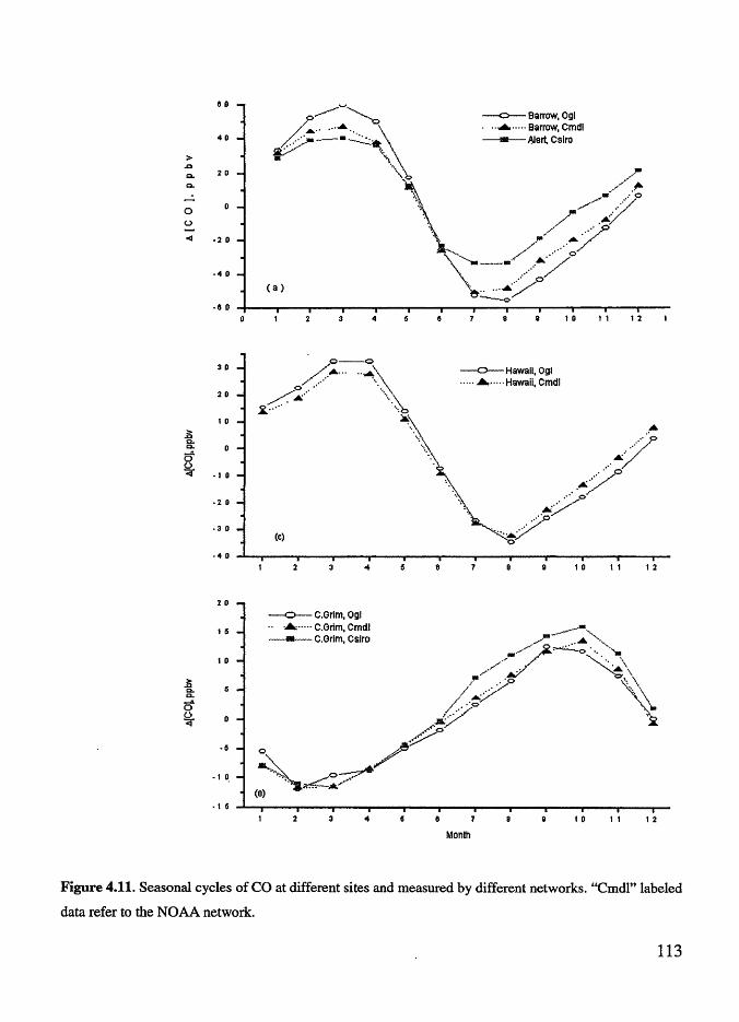
G II
411
> ..Q
Q.. 2 0
Q..
.....:. 0 0
-<I • 2 II
.4 II
·II II
311
2 II
1 II
A Q. Q.
cf ~ • 1 II
·2 0
.3 0
·4 II
2 0
1 ('i
1 II
1l a.. Q.
cf (.)
<r
.(I
·111.
• t G
Ca)
4
(c)
-0-C.Grlm, Ogl .. . .......... C.Grim, Cmdl
----- C.Grlm, Cslro
--o--Barrow, Ogl . .. ..... · ·· ·· Barrow, Cmdl -----Alert. Cslro
1 II
-o--Hawaii, Ogl .............. Hawaii, Cmdl
1 II
111
Month
11 1 2
11 1 2
11 1 2
Figure 4.11. Seasonal cycles of CO at different sites and measured by different networks. "Cmdl" labeled
data refer to the NOAA network.
113

After making the calibration adjustments, we constructed the seasonal cycles
(these are the d8(m(t))from Eq. 4.2) for all sites and networks (Fig. 4.11) as well as the
12-month moving averages ( C(t) ), which are plotted in Fig. 4.12. With the exception of
the South Pole, there is good agreement between the OGI and NOAA-GMD cycles at
all sites. The May peak in CO observed in the OGI South Pole data is not a permanent
feature of the seasonal cycle, rather it can be attributed to high concentrations during
this month in 1986 and 1991. These years have a disproportionate.weight to the
seasonal average as there are significant gaps in the OGI South Pole record, and the
interpolated data covering these periods are not used to derive the seasonal cycle.
The seasonal cycle measured at Alert, Canada, by the CSIRO network has a
smaller amplitude than observed at Barrow from the other networks·. As Alert
(lat=82.5°N) is considerably more north than Barrow (71.3°N), the summertime trough
is shallower since OH levels decline with higher latitudes and reduce the oxidation sink
of CO at Alert. At the other two common sites, Cape Grim and the South Pole, we see
good correspondence in the phase of the CSIRO cycles, though the peak-to-peak
amplitude is larger. This occurs because the global scaling factor used to calibrate the
CSIRO data underestimates the true difference here, producing a residual calibration
difference of about 2% (in the direction that CSIR.0-CO is higher than NOAA). As this
is a polar site, the small discrepancies here will not significantly impact our findings in
the tropics.
114

'10 s 160 ........
~ = 120 0 u cO 80
< 40
(a)
--Ba now, OGI _________________________________ _
- .... - . Banow,NOAA-GMO
-·-Alert, csnw 0-'---.-~---+--------.--~....--....-.....-4--.---.--.--+--r--,----r-t--r--r--r--1
1980 1984 1988 1992 1996 2000 2004
'10 s 160
] = 120
8
.. ~\
------------------------------:~-,,,~2~\~~ ---cO 80
< 40
--C.Meares,OGI
- . - - ••. C. Meares+others, NOAA-GMO
-·-Est.Pt.,CSJRO
Q+---.---.--..---+---....--.---.--~.---.--.--l--..--.--.--+--.----i--..--+-...--r--r-~
1980 1984 1988 1992 1996 2000 2004
'10 s 160
(c)
] ~ 120
8 ~ 80
< > 40 ~
- --Hawaii, OGI - - - - - - - -· - - -- - - - - -- - - - - - - - - - - - - - - - - - - -- • - ..•. Hawaii, NOAA-GMO
-·-MLoa,CSJRO 0 4---.--.--.---+--..--.-..---1--.....--.---.--1--.---.----..~1-...-......--....--1--,.--.----r---l
1980 1984 1988 1992 1996 2000 2004
Figure 4.12. Adjusted CO records at different sites and by different sampling networks. The data plotted
are 12-month moving averages that have been scaled by the appropriated calibration factor to place
measurements on the NOAA-GMD standard. (a) north polar, (b) north mid-latitudes, (c) north tropics.
115

70 s 160
~ i::::: 120 6 u bD 80
< > 40 0
~
(d) --Samoa, OGI
....... samoa,NOM-GMD
-·-Cape Ferg.,CSIR.O
o+--.--..---,--+----r--r-~-+--.---.---r--+--,-.--,...-+--.---.---.--+-~~--,-~
1980 1984 1988 1992 1996 2000 2004
200-.-------------------------~
70 (e) --Cape Grim, OGI ....... Cape Grim, NOAA-GMO
-·-Cape Grim, CS IRO
s 160 ---~ i::::: 120 -~ c5 u bD 80 -~
< > 40 -~ 0
~ 0
1980
....... I
I I I I I I I I
1984 1988 1992 1996 2000 2004
(f) --S.Po~.OGI .... - .. S. Pole, NOAA-GMO ~ 1()() -- -- - -- - -- - ~ --- - - - -- - -- - - - -- - -- - - .. ~- -· ·- ·- --- -- -- - . -
~ -·-S.Pole,CSIRO
i::::: 120
g bD 80
< > 40
~ ,,_,_-.,.....'.••••.·••".!"·'''~~·~ ..... ! ....... OJ ..... .--
O-t-.....--.--,--+--.-~--.---+---...---...--,___,--,,--,--,--;--.,---.-.--+---,--,--,..--i
1980 1984 1988 1992 1996 2000 2004
Figure 4.12 (cont). (d) south tropics, (e) south rnid-lati~udes, and (t) south polar region.
116

We next compared the calibrated moving averages at each site from all networks
(Fig. 4.12) to assess whether it is feasible to composite records from different networks
into a single long term time series. It is evident from this figure that the latitudinal
gradient measured by the OGI network is in excellent agreement with NOAA-GMD
measurements. Though overall the moving average records for all sites show few
features, the "hump" observed from 1993-1997 in the northern mid-latitudes is seen in
both records. In addition, the slight interannual variability over the same time period at
Hawaii is also evident in both records. There is also good correlation between the small
features in the South Pole records. We conclude that the OGI.and NOAA records are in
close enough agreement to create a composite CO time series that spans from 1981 to
2004. To our knowledge this is the longest CO time series that has been constructed.
We inverted this composite time series below to estimate the CO emissions over this
time period.
4.3.4.2 Hydrogen As we mentioned above, the hydrogen record shows some interesting behavior
over the time span of measurement (Fig. 4.7). Broadly, this behavior is seen across all
networks. During the period of measurement overlap between the OGI and CSIRO data
sets, H2 levels rise from a minimum in 1994. This rise is captured in both data sets. The
OGI data set finishes just after H2 peaks in 1996-97. The CSIRO measurements, which
extend past this time, reveal that this peak sits on the shoulder of a broader feature that
peaks a couple years later in 1998-99. After this CSIRO-H2 levels fall rapidly by 4-5
ppbv f 1 until the record ends in 2002.
117

1.03
~ 1.00
~ 0.98
'iii (..) 0.95
0.93 (a)
- Alert - Mloa
-CGrim -SPole
0.90 +----.----r---,-----,-------.-----1
1990 1992 1994 1996 1998 2000 2002
1.05 -,------------~----------.,
1.03
"'C 1.00 E Q 0.98 'Ci 0 0.95
0.93
- Barrow - C. Meares - M. Loa - C. Kumukahi - Samoa -C. Grim
- S. Pole 0.90 +----r"-~--r----,,-----,-----.-----1
1.05
1.03
e 1.00 '(ii
Q 0 .98
8 0 .95
0 .93
1990 1992
(c)
1994 1996 1998 2000
M . Loa
-C. Grim
S. Pole
2002
0 .90 +-----------,---------~------<
1990 1992 1994 1996 1998 2000 2002
Figure 4.13. Evidence of a calibration drift is seen in the time series of calibration ratios. Plotted are the
ratios of (a) CSIRO H2 to NOAA-GMD (Cmdl), (b) OGI to NOAA-GMD, and (c) OGI to CSIRO. Ratios
are derived using measurements from common sites (labeled). ratio of H2 data between different
networks.
Consistent with the OGI record, NOAA H2 also falls from the start of the record
in 1989 to a minimum in 1993-94 and then rises again to another peak in 1996.
118

However unlike the OGI record, H2 levels do not rebound back to 1989 levels after the
1993-94 minimum. The OGI record indicates that H2 levels are comparable in 1988-89
and 1996-97. Even past this 1996-97 peak, NOAA H2 never returns to the levels at the
beginning of the time series in 1989. Because of this, there is an overall downward
trend in the NOAA H2, which is not present in the records from the other two networks .
. In part this is due to a drift in the calibration seen in the NOAA-GMD and
CSIRO H2• This drift can be seen in the inter-network comparisons of H2 shown in Fig.
4.13. Here we plot the time series ofCSIRO/NOAA, OGl/NOAA, and OGl/CSIRO
ratios of H2 for all sites in common between networks. The largest drift in calibration
exists from 1992 to 1997 between the OGI and NOAA measurements. Over this
interval, the calibration ratio increases from 0.94 to 0.99 for a trend of 1.23% f 1. A
trend also exists, though smaller, in the ratios from the other two network
intercomparisons. We calculated a trend of 0.67% f 1 and 0.60% i 1 for the OGl/CSIRO
and CSIRO/NOAA ratios. Since all intercomparisons reveal a trend in the calibration,
there must be a drift in the calibration for at least two networks. Since the CSIRO scale
is based on NOAA standards, it seems reasonable that the calibration standard for both
networks is drifting. If so, and if the OGI standard was stable, then from 1992 to 1997
the NOAA calibration drifted downwards at a rate of -1.23 % y-1, and the calibration
for the CSIRO data declined by --0.6% i 1•
After 1997 the calibration stabilizes and the CSIRO/NOAA ratio is close to
unity during this time. We adjusted the OGI measurements to the NOAA scale
correcting for this drift. We use caution when interpreting the emissions inverted from
119

40
30
20
10
i 0
~-10 <I -20
-30
-.CD
10
l 0
~ <I
-10
-o-OGI .-•· --.l - •·· NOAA-GMO
~~~~,········-. ... -+-CSIRO
/ ~' \: _.,/ ..
~ (a) North polar ,,..
5 6 7 B 9 10 11 12 13 ........ .... -:::: ·· ... .··.:;,.&:,::_::;:;:f~~-.
.... / ·····~ / "·.~· ,,.-;i .• ~·· •/'' · .. fl'" .•. "• ..
\"·•? ... ~
(c) North tropical \:. ....... ..
-20 -+--r--..---.--.----r---,----r---.-----.-~~--r---.
30
20
10
l 0
g. -10 <I
-20
-30
35
30
25
20
3 4 5 6 7 8 9 10 11 12 13
15 5 6 7 B 9 10 11 12 13 20 1 10 11 12
l ;?:
10
<I -5
-10
(e) South mld-lelltudes -15 +---T---.---.--.--......--.----r---.-----.-...---.---T---.
0 5 8 B 9 10 11 12 13
16
10
.i!: 5 8: ~o <I .5
·10
(f) South polar
3 ' 6 6 7 8 g 10 11 12 13
Figure 4.14. Seasonal cycles of H2 at different sites and measured by different networks. The sites for
each region are (a) Barrow (OGI, NOAA), Alert (CSIRO); (b) Cape Meares (OGI, NOAA), Est. Pt.
(CSIRO); (c) Mauna Loa for all three, plus Cape Kumukahi (OGI, NOAA, avg. with M.Loa); (d) Samoa
(OGI, NOAA), Cape Ferguson (CSIRO); (e) Cape Grim (all); and (f) South Pole (all).
the measurement record from 1992 to 1997 from the NOAA and CSIRO networks. We
note that the OGI measurements span this period of concern, and we generally base our
conclusions on the OGI record during this time.
Despite absolute calibration differences, there is good agreement of the seasonal
cycles of H2 measured at each station (Fig. 4.14). The timing of the peaks and the
troughs is consistent between networks at all sites except at the north polar sites where
120

the minimum of the seasonal cycle for each network occurs at a different month. The
minimum at Alert occurs a month earlier than at the NOAA Barrow station, which in
tum occurs a month earlier than at the OGI Barrow location. Since the minimum is
largely determined by the soil sink, it is reasonable that the shorter growing season at
Alert would produce an earlier minimum than Barrow is southward. It is unclear why
the timing is different for the other two networks as both are sampling air from the same
station. The cycles indicate the H2 maximum is reached during April and May
throughout the northern hemisphere, and during December and January in the southern.
The minimum in the northern hemisphere occurs at later dates in the year for southern
sites showing the dominance of the destruction term. We also observe that the
amplitude of the seasonal cycle is largest at the higher latitudes in the northern
hemisphere, again consistent with the strong seasonality of the climate there and large
land mass area, both which determine the strength of soil uptake. In general the
amplitude of the cycle is largest for the NOAA-GMD measurements. This is consistent
with our finding that the NOAA-GMD absolute calibration is higher than the others
during the period of overlap.
4.3.5 Composite record We show the composite record of CO in Fig. 4.15. This was created by joining
together the scaled OGI and unscaled NOAA-GMD measurements. During the period
of overlap, monthly averages from each site were weighted by their respective standard
deviations and the weighted average was determined. The monthly data are decomposed
121

-- Barrow - North mid-lat. Hawaii -- Samoa - - Cape Grim -- South Pole
60
-60 (b)
Year
1 2 3 4 5 6 7 8 9 10 11 12
Month
Figure 4.15. Composite time series of CO using measurements from the OGI and NOAA-GMD
networks. (a) Deseasonalized time series at the major latitudinal sites. (b) Average seasonality of the
composite record at each site.
into two components: the deseasonalized data, C(t)-11.(m(t)), and the seasonal cycles
11.(m(t).
The deseasonalized CO composite series stretches from Jan 1981 to Dec. 2003,
a twenty-three year time span. Besides the variability and departures from the average
seasonality seen in the time series, the most notable feature is the trend, and the change
in trend with latitude. The trend for each site was computed over the entire time span
(Table 4.3). We find two different behaviors of the CO concentrations at the different
sites; large decreases and negative trends for Barrow and Cape Meares, (- 1.01±0.14 %
f 1, and-0.86 ± 0.17 % y-1
, respectively, where the uncertainties relate to 90%
confidence intervals), while the more southerly sites show little to no decrease (the
trend ranges from -0.07 % f 1 to -0.31 % f 1). The trends at the sites reflect
122
predominately changes in local sources and sinks owing to the relatively short lifetime
of CO (,.., 2 months).
Trends can be produced in the atmospheric record by changing sources and/or
sinks, or perhaps a mixture of the two. More information about the nature of the trend
can be obtained.by looking at the pattern of the seasonal cycle strength over these years.
We calculated the cycle strength in the following manner. For each site we selected a
three-month window centered on the cycle maximum and a window centered on the
cycle minimum. For each year we found the maximum and minimum concentrations
that fall within the windows. We defined the cycle strength to be the difference between
these two values.
123
t I
I I
I .I
I !

(e) (b)
200-(C) .
....-<r-mlnlma 240- /"'O'O -o- maldme
240 0
1~ V'°\, ........._peak-to-peak tA· 0
100-220 220
0
200 0 "o'o l 200 "<>'o,.o"o 1SO
~ \"O \A, ,f\ ,,J\~p•f \,,._~ ~ 180 'o"O)>\ 180 1411-
.g_ 160 '-b-0
160- 'b V\P'° l-o'o-o V\ a. 120
5' 140
pr-\r..._ 140 "' 2. ;~
100
120 120- }\-<'\ ·15 c "':V.~~4»4A ? ........... , ... liO
100 /'qr"\•-c-u.P'D\, ,,.!:I~~'. 100 oA~ "./·>.1.1'\fx.;_
80 . ..a.., \ 'ti~ 80 EiO I I' l·• ",. '-'\ D~ :t;
60 60 40
1980 1984 1988 1992 1996 2000 2004 1980 1984 1988 1992 1996 2000 2004 1!BI 1984 1988 1992 1996 2000
Year Year Year
Figure 4.16. Analysis of CO seasonal cycles in the northern hemisphere. As described in the text,
minimum and maximum values of the seasonal CO cycle were determined from the composite record.
Peak-to-peak values is the difference between the two. (a) Barrow, (b) Cape Meares, (c) Hawaii.
Fig. 4.16 shows the trend of the cycle strengths for the sites in the northern
hemisphere. At these sites the cycle strength decreases faster than the decrease in
GOncentration (-2.1, -2.3, and -1.7 % f 1 vs. -1.0, -0.86, and-0.14 % f 1, respectively
from north to south). Furthermore we see that it is the fall in the cycle maxµna that
causes
20J4
124

Table 4.3. Trends of the CO composite time series
Location Deseasonalized Cycle Cycle Cycle D trend Strength maxima minima (maxima - minima)
% yr·l % yr·l % yr·l % yr·l % yr·l
Barrow -1.01 -2.08 -1.50 -0.79 -0.70 (0.14)a (0.32) (0.36) (0.49)
Cape -0.86 -2.34 -1.29 -0.15 -1.14 Meares et (0.17) (0.39) (0.45) (0.60) al. Hawaii -0.14 -1.66 -0.62 -0.38 -1.01
(0.10) (0.39) (0.50) (0.64) Samoa -0.07 0.99 0.00 -0.68 0.38
(0.07) (0.53) (0.75) (0.73) Cape Grim -0.22 -0.45 -0.59 -0.68 0.10
(0.06) (0.48) (0.75) (0.89) South Pole -0.31 -1.68 -0.98 -0.30 -0.68
(0.15) () (0.70) (1.14) (1.34) a Values in parenthesis are 90% confidence limits
the strength to decrease with time as the cycle minima remain constant or nearly so. For
these three sites the trends in the maxima are negative and are significantly different
than the respective trends in the minima at the 90% confidence level (Table 4.3). This is
not the case for the three southern hemisphere sites. From this fact we conclude that the
reason for the drop in CO concentrations is due to a fall in its sources rather than an
increase in its sinks. An i~crease in CO's sink, i.e. in the concentration of the hydroxyl
radical, would not only decrease the cycle's maxima but also its minima. Though a
decrease in CO source would decrease the cycle's minima, it would have a greater
impact on the cycle's maxima, since the maxima represents an integrated sum of CO
emissions over the months when the lifetime of CO is long, namely the winter season,
whereas in the summer the concentration of CO is more a reflection of acute emissions
due to the short lifetime of CO during these months. Thus the observed decrease in CO
125

cycle strength must be in response to diminishing CO emissions in the northern
hemisphere.
Table 4.4. Trends of the Hi composite time series
Location Deseasonalized Cycle Cycle Cycle A. Trend % yr·l Strenyth Maxima Minima (maxima - minima)
%yr· % yr·t % yr·t % yr·l
Barrow -0.94 -1.2 (1.4) -0.34 -0.21 -0.12 (0.14) (0.10) (0.21) (0.24)
Cape Meares -0.45 -1.4 (1.9) -0.27 -0.15 -0.11 et al. (0.12) (0.10) (0.19) (0.21) Hawaii -0.20 1.3 -0.08 -0.15 0.07
(0.10) (2.8) (0.10) (0.13) (0.17) Samoa 0.28 . -0.02 0.01 (0.10) 0.01 (0.09) 0.00
(0.08) (2.9) (0.14) Cape Grim 0.37 (0.08) -0.15 -0.01 0.01 (0.09) -0.01 (0.14)
(2.8) (0.10) South Pole 0.24 (0.08) -1.5 -0.03 0.04 (0.08) -0.07 (0.13)
(1.8) (0.10)
There is somewhat different behavior in the hydrogen composite time series
than observed in the CO data. There. are again significant negative trends in the
deseasonalized data in the northern hemisphere, but in the southern hemisphere where
CO was also decreasing, we observe hydrogen to be increasing slightly but statistically
significant (Table 4.4). Whereas the average CO trend in the NH is-0.51±0.07 and-
0.18 ± 0.04 % t 1 in the SH, for hydrogen we find the average NH trend is -0.44 ± 0.07
and the average SH trend is 0.30 ± 0.05 % t 1•
In addition, we find different behaviors in the cycles. There is no significant
decrease in hydrogen cycle strength, nor is there any significant difference betwee~ the
trends in the minima and maxima in either hemisphere (Table 4.4). Rather we find the
averag~ minima and maxima trends in the NH are both negative and are both positive in
126

the SH, thereby producing a nearly constant cycle strength throughout this period in
both hemispheres. Also the average NH maxima trend is significantly different than the
SH maxima trend and likewise for the minima trends.
We found above that the observed behavior of CO can be explained by a
decrease in its sources. Since the sources of CO and H2 are similar, it follows that H2
sources are also decreasing. Though the behavior of H2 is different than CO, decreasing
emissions are consistent with the observed trends considering the lifetime of H2 is more
than ten times greater than the lifetime of CO.
4.4 Modeling
127

Inverse modeling exploits the mass balance equation to estimate emissions
based on the atmospheric record of a gas. For a one-box model, the mass balance
equation can be written
(a·n) :: =S-(a·n)~, (4.4)
where xis the globally-averaged volume mixing ratio of the gas (e.g nmol mor1), S is
- - Barrow Cape Meares et al. Hawaii - - Samoa -- Cape Grim -- South Pole
560 40
30
540 20 ---- ................ . ,
- --- ..__l'--.·~ ~\ 520 10
• l l. l.
~ §: 0 \ :;/
\ ·-:?. 500 ~ -10 :..
<I -20
480 -30
(a) (b)
460+--.~--.-,c-----.-,--~-.--~~.---~-.---,-~ 1984 1988 1992 1996 2000 2004 1 2 3 4 5 6 7 8 9 10 11 12
Figure 4.17. Composite time series of H2 using measurements from the OGI and CSIRO networks. (a)
Deseasonalized time series at the major latitudinal sites. (b) Average seasonality of the composite record
at each site.
the emissions per time interval (e.g mol f 1), ris the lifetime of the gas, and n is the size
of the atmosphere in moles (mol), and a is a conversion factor that translates, in this
example, nmol to mol. If the temporal record of x is known, the equation can be
"inverted" for the global emissions S
128

(4.5)
In practice -c will be a function of time since removal processes are rarely spatially or
temporally homogeneous. Nonetheless the above equation gives a good first order
approximation of global emissions. Here we wish to estimate e~ssions over specific
geographical regions where biomass burning is most prevalent so the one box model
approach is not appropriate.
In principle w~ can apply the above equations to any homogeneous volume of
atmosphere, within which the mixing ratio and lifetime are spatially constant. This
volume element or "box" is considered well-mixed, which requires that transport.times
are short enough to overcome small spatial differences in sources and sinks. The major
complication that arises when adding spatial resolution to the one-box model of Eq. 4.4
is the transport of the gas into and out of the volume element. This transport can be
roughly categorized as either turbulence or advection. Adding transpon processes, the
one box model above becomes
ax =T-V ·((x)(v)+ K · ci~). dt dx
(4.6)
Here T represents both the sources and sinks of the gas and the second term on the right
hand side is the transport processes. Advection is characterized by the mean flow v, thus
the first term in the brackets is the flux of the gas across the boundary of the volume
element. The second term in the brackets specifies turbulent flow characterized by the
eddy diffusivity coefficient K. Since our model has two spatial dimensions K is a two-
dimensional matrix. Turbulent transport is then the product of K with the mixing ratio
129

gradient az/a;. Mean winds and eddy coefficients were derived from meteorological
data (Butenhoff, 2002).
By integrating Eq. 4.6 over well-mixed volume elements and using matrix
methods Eq. 4.6 can be written as
dx =S+nx. dt
Here the bold style denotes a one or two-dimensional matrix and n is a two-
(4.7)
dimensional matrix that contains all the transport and lifetime terms. The solution to Eq.
4.7 is
I(t) = 10
exp(Ut) + n-1s[exp(Ut)-I], (4.8)
where I is the identity matrix. The equation can be inverted to find the emissions S,
S = (expilt-It1n11 -(expilt-Jt1U(expilt)1°. (4.9)
Here 11 and 1° are the current and initial mixing ratios, respectively. As written, S
includes sources from all model boxes. For our purposes we are only interested in
emissions into the surface model boxes since this is where biomass burning occurs.
Both H2 and CO have non-surface sources due to oxidation processes. Emissions from
these sources will not be part of the model inversion, rather we include them into the
simulation. To accommodate this, we split Eq. 4.8 into two equations, one equation for
surface emissions, and the other for non-surf ace emissions. To simplify notation we
define
130

G = (exp flt - I t1, X=exp!lt,
S = surface boxes,
N = non - surface boxes,
and T = all boxes.
(4.10)
In the following equations, the subscripts refer to the dimensions of the matrix. We also
drop the bold style for convenience as the subscripts clearly denote matrices. With this
notation the emissions from the surface boxes are found by
(4.11)
and the emissions from the non-surface boxes are
(4.12)
Since we do not know z1 (the current mixing ratios in the non-surface boxes) a priori,
but do know the emissions here, we rearrange Eq. 4.12 to solve for z1:
(4.13)
All terms on the right hand side are known. SN is the emissions from oxidation of
methane and other hydrocarbons in the upper troposphere, and z~ is the surface mixing
ratios of CO and H2 known from measurements. By calculating z1 and supplementing
with z~ , we can construct z~ , which then allows us to calculate the surface sources Ss
in Eq. 4.11. Note that the inverted surface emissions will still include the oxidation
products in the lower troposphere. These we remove a posteriori. In the next two
sections we discuss the modeling of the removal process of both gases, and emissions of
H2 and CO from oxidation of hydrocarbons.
131

4.4.1 Sink processes Reaction with OH is about 90% of the total CO sink but is responsible for only
about 5% of hydrogen's total removal. To model the OH sink, mqnthly OH fields were
taken from Spivakovsky et al. (2000) and averaged over the mass balance model
latitudinal and altitudinal boundaries The reaction rate coefficient between OH and CO
is pressure-dependent and specified as kco+oH =l.5xl0-13 (1+0.6p[atm]), (DeMore et
al., 1997). We also include the loss of CO and H2 by stratospheric oxidation using the
stratospheric OH fields of Bruhl et al. ( 1990 ).
Soil uptake by biological processes is the dominant removal mechanism for
hydrogen, representing some 90-95% of its total sink (Warneck, 2000). Soil uptake is
less important for carbon monoxide, but still accounts for about 5-17% of its total sink
(Conrad and Seiler, 1985). The removal of atmospheric CO and H2 by soils is due to
the oxidation of these gases by soil bacteria (CO) and extra-cellular enzymes (H2)
(Yonemura et al., 2000). Field studies indicate that deposition rates vary little with
temperature (R2=0.171, 0.150, 0.05, from a field study in Japan; Yonemura et al, 2000),
but fluctuate strongly with soil moisture, being lower in moist soil conditions
(Yonemura et al., 1999, Yonemura et al., 2000; Conrad and Seiler, 1985). Yonemura et
al. (2000) reported R2 values of 0.861 (CO) and 0.676 (H2) between deposition
velocities and soil moisture over a limited range of soil moisture levels (soil moisture
content, r~tio in volume, =0.2 to 0.4 ). This observation is likely a result of a reduction in
the exchange of air between the atmosphere and soil when soil pores are clogged with
water (Conrad and Seiler, 1985). Soil moisture lev_els may also affect rates of microbial
132

activity (Shuler and Conrad, 1991). Conrad and Seiler ( 1985) estimated global
deposition values of 7 x10⁻⁴ m s-1 for H2 and 3 xlff4 m s-1 for CO.
There is little information about the seasonal or regional patterns of either H2 or
CO deposition. Previous studies have used net primary production (NPP) as a proxy to
allocate deposition velocities spatially (Hauglustaine and Ehhalt, 2002; Muller and
Brasseur, 1995). Though primary production is influenced by soil moisture, it also
depends on sunlight, nutrient level, and temperature, variables that are not expected to
influence deposition.
Instead of NPP, we used soil moisture to model the variability of deposition. We
used 0.5x0.5° maps of soil moisture from the University of Delaware Climate Resource
Center (data downloaded from
http://gcmd.nasa.gov/records/GCMD_UDEL_CSD.html) Soil moisture is quantified as
an index between-1 (dry) and 1 (saturated) on a monthly cycle from 1950 to 1999. For
simulation years outside this range, we used a mean seasonal climatology.
We transformed the soil moisture indices (SMI) to deposition velocities (V)
using a logistics equation of the form
v = AVO BV+(A-BV
0exp(-A·SMI)'
(4.14)
where A and B are constants and related by B=AIV nuzx, and V max and V0 are the maximum
and minimum deposition velocities, respectively. The use of the logistics equation
ensures that the deposition velocity stays within a specified range which was
determined from the literature, and that the relationship between soil moisture and
133

deposition is nearly linear over much of the range of soil moisture which is consistent
with the field studies of Yonemura et al. (2000). V~ = 0.14 and 0.07 cm s-1
respectively for H2 and CO, and V0 = 0.01and0.05 cm s-1 respectively for CO (Conrad
and Seiler, 1985; Yonemura et al., 2000). The constant A was adjusted until the global
median was equal to 0.07 cm s-1 for H2, which was reported by Conrad and Seiler
( 1985 ). The same value of A (2.2) was used to compute the CO deposition velocities.
The mean seasonal cycle of H2 deposition velocities based on soil moisture only are
plotted in Fig. 4.18 for each model region. Deposition velocities are highest during the
summer months of the northern polar and mid-latitudes.
134

0.12
0.10
0.08
~ >~ 0.06
0.04
2 3 4 5 6 7 8 9 10 11 12
Month
---np ----nm -.t.-nt ~st --+---sm --.c- sp
Figure 4.18. Average seasonality of H2 soil deposition velocities for the six latitudinal regions of our
simulation. n=north, s=south, p=polar, m=mid-latitudes, t=tropics. Month l=Jan, 12=Dec.
Past work has found that deposition velocities go to zero when soils freeze
(Bergamaschi et al., 2000) and when the temperature exceeds 40°C, which is too high
to support relevant microbial activity (Liebl and Seiler, 1976). Globally gridded lxl 0
maps of monthly average surface temperatures were used to filter out dates and pixels
meeting these conditions. Non-soil land types such as permanent wetlands, snow and
ice, and water bodies were removed from area estimates using the lxl 0 MODIS Land
Cover Product which includes 17 different land cover categories (Strahler et al., 1999).
We also excluded deserts and barren lands as soil moisture needs to be at least 5-10%
for deposition to occur (Conrad and Seiler, 1985). From the filtered data set, a time
series of frost-free land areas was derived for use in calculating soil uptake over the
135

model regions. We assumed the areas of the land cover types were not seasonally
dependent.
4.4.2 Oxidation of methane Methane and non-methane hydrocarbons (NMHCs) react with atmospheric OH
and produce a number of oxidation products, including both CO and H2. Oxidation
occurs throughout the atmosphere meaning some CO and H2 will be produced in both
the lower and upper tropospheric layers of our model atmosphere. Before inverting the
CO and H2 records, we need to include these emissions of CO and H2 from oxidation
into the model, otherwise simulated surface fluxes would be forced in error to account
for this atmospheric production. According to the above notation, emissions of CO and
H2 in non-surface boxes are labeled SN.
The first stable product from the Clti+OH reaction is formaldehyde (CH20).
The photodissociation of CH20 has two branches, one that produces both CO and H2
directly,
(Rla)
and a second branch that produces HCO by
CH20 +hv -7 HCO + H, (Rlb)
which is then oxidized to CO:
HCO +02 OH 4 H02 + CO. (R2)
The oxidation of formaldehyde by OH also.leads to CO through the intermediary
product of HCO
(R3)
136

The fraction of CH20 that is oxidized decreases with altitude due to decreasing OH
levels. Warneck (2000) estimated that about 40% of the CH20 produced from CH4+0H
reaction is oxidized. Of the fraction that is photolyzed, branch la occurs about 68% of
the time.
"";'" 200 >. C>
...... 6 {) 100
----~---
1975 1980 1985 1990 1995 2000
100
"7>C> 50
......
g 0 t:=:~~~---t~==i >
-50
1 2 3 4 5 6 7 8 9 10 1112
-np
-nm
· · nt
-st -sm
-sp
Figure 4.19. CO production from C~ oxidation. (a) 12-mo moving avg. of CO production from C~
oxidation. (b) Seasonal cycle of CO production averaged over time series. n=north, s=south, p=polar,
m=mid-latitude, t=tropics.
Formaldehyde is water soluble and can be scavenged by rain before conversion
to CO. From inverse modeling studies, Bergamaschi et al. (2000) estimated an average
CO yield of 86% from methane oxi~ation, and we adopted that figure here. We
calculated a time series of CO production from the C~+OH reaction using the
composite OGI-NOAA methane record and the monthly OH fields from Spivakovsky et
al. (2000) For the upper troposphere where no systematic measurements exist, we
scaled surface concentrations by 0.9 to account for the slight vertical gradient. Over the
137

entire time interval (1981 - 2004), the average loss rate of C~ due to OH oxidation
was 473 Tg y-1.
This compares well with the range of global loss rate cited in the 2007 IPCC report
(425-511 Tg i 1) (Denman et al. 2007). We computed CO production by scaling these
emissions by the 0.86 factor above and multiplying by the ratio of molecular weights
(28.01 g mor1/16.0 g mor1). We found on average annual CO production from
CH4+0H oxidation was 826 Tg i 1• This is quite close to th~ value of 830 Tg y-1
estimated by Bergamaschi et al. (2000 ). The CO production for all surf ace model
regions is plotted in Fig. 4.19 along with the average seasonal cycle. Consistent with the
atmospheric methane trend, the CO produced from the Cl4 oxidation has been nearly
constant in past years. We estimated that 75% of the total CO production occurs in the
tropics, and only 1 % in the polar regions.
The H2 production was found by
s H2 (t) = 0.68. 0.60. '}5CH4 (t). (M H2 IM CH4 ), (4.15)
where 'Y is the fraction of CH20 not removed by scavenging, 0.6 is the fraction of CH20
photolyzed, 0.68 is the quantum yield of branch a, and SCH4 (t) is the time series of c~
oxidized as calculated above. From this we calculated an average production of 25 .4 Tg
i 1. This is comparable to the estimate of Wameck (2000) of 20 Tg i 1•
4.4.3 Inversion
Due to latitudinal gradients, H2 and CO levels are not constant through the
volum~ elements represented by boxes in our model. To account for the small mixing
138

ratio gradients we integrated the latitudinal profile z( (}) over the latitudes ( 8) of each
model box i,
(4.15)
In practice we do not know the mixing ratios at the boundaries of each model box (i.e.
81 and fh.). Instead we interpolate values using the mixing ratios ~t neighboring sites. In
this manner the modified mixing ratio Xi reflects the true abundance of the gas in each
model box. This adjustment has the greatest impact in the tropics boxes where the
interhemispherical gradient lowers the effective mixing ratio in the north and increases
it in the south. In the vertical direction, observations indicate that the mixing ratios of
CO and H2 remain nearly constant in clean air where there are few surface sources
(Emmons et al., 2004; GTE aircraft,). The vertical profile is maintained by production
of both gases at altitude by oxidation processes.
The mathematics of our mass-balance transport model allowed us to invert the
time series of atmospheric concentrations directly without recourse to an optimization
scheme. To do so, we needed to describe the state of the atmosphere with regards to the
CO and H2 mixing ratios at the date of initialization. We did this using an a priori set of
emissions that are optimized so that model-simulated mixing ratios are consistent with
the observed mixing ratios at the beginning of our time interval in the surface boxes. If
we run this simulation for a number of years, mixing ratios in the upper troposphere and
stratosphere come into steady state with the mixing ratios in the lower box. This steady-
state field of mixing ratios was then used to initialize consequent model runs.
139

The output of the model inversions was monthly surface emissions of CO and
H2 distributed by latitude. Our focus here was primarily on the tropical boxes spanning
the region from 30S to 30N. The reason for this was twofold. About 90% of global
biomass burning occurs in the tropics dominated by savanna, grassland, and biofuel
burning. And secondly, biomass burning is the dominant surface source of CO and H2
in the tropics. Thus the record of CO and H2 emissions that we inverted from the
atmospheric record should largely reflect the variability and trend of biomass burning.
4.5 Source deconvolution
140

The deconvoluted CO and H2 emissions are presented in Fig. 4.20. A comparison
of CO and H2 emissions is shown in Fig. 4.21 for the ST region. They include all
emissions in the lower tropospheric boxes. This includes not only surface fluxes but in
"';->. Cl I-c5 (.)
(j)
';" >. Cl I-
N" I
(j)
3500
3000
2500
2000
1500
1000
500
0 1980
160
140
120
100
80
60
40
20 (b)
-Global ---- -- -_-_-N_H_, ______ :::s_H _____ --i
' •' .. , ;·:·: : I .. ..
' .. :'
' .. :
1985
-Global . .. \ ..
•' ' ,, :' . . I :
'
1990 1995
--NH
• ' .. ' .. .. , ..
I
'
,. ,,. ...
•"
" " 1, I ' I
2000
I
2005
----~
: : .... " '· ... I ~ I O f I I .. : ·.
O+-~-.,--,--,----J-.,---,---r-~-+--~--,.-~-,--+--r-~-,-~--+-~-,--~~-+----,-J
1984 1988 1992 1996 2000 2004
Figure 4.20. Simulated (a) CO and (b) H2 emissions based on our inversion. The solid lines are 12-month
moving averages of the average monthly source strengths (dashed lines). Emissions are shown for global
(black), northern hemisphere (blue), and southern hemisphere (black) totals. Data shown include all
sources of emissions except for production in the upper troposphere from Ciii oxidation.
141

1200 ---· --- - - --- ----- - - - 70
1000 60
... 800 50 ... a ~ N
0 ::c en 600 40 C)
I- I-
0 N :c u 400 30 en en
200 20 --co --H2
0 10 1985 1990 1995 2000 2005
Figure 4.21. Simulated emissions from inversion for the south tropical (ST) region.
situ production of CO and H2 from the oxidation of both CH4 and NMHCs in the lower
troposphere. Production in the upper troposphere is not part of the total.
We estimated the total CO source strength is 2210 Tg i 1• If we included the CO
from the CH4+0H reaction in the upper troposphere, this increased to 2340 Tg i 1• This
is within the range of recent estimates if not on the low end (Khalil and Rasmussen,
1990; Pacyna and Graedel, 1995; Hauglustaine et al. 1998; Bergamaschi et al., 2000).
The inverted records also indicate the predominance of northern hemisphere (NH)
emissions to the global total. We estimate that CO production in the NH is 2.3 times
higher than in the southern hemisphere. This is primarily due to the burning of fossils
fuels in the transportation and industrial sectors.
142

There is an evident downward trend to the global CO source strength that begins
in 1988 and continues to the end of record. Though there is a small trend in the SH
emissions from 1988 to 1993, the emissions past this point remain nearly constant. The
global trend is for the most part caused by the behavior of CO in the NH. If we remove
the positive anomaly in the NH CO around 1997, the CO trend from 1998 to 2003 is -
0.7 % y-1• Over the course of this period, this is a decline of 11 % or about 270 Tg CO y-
1. The most probable reason for this is the reduction of CO emissions from vehicles.
The U.S. Environmental Protection Agency estimates that CO emissions from on-road
vehicles (i.e. cars, light and heavy trucks, etc.) have declined by 40% since 1970 (EPA,
2010).
The coincidence of the seasonality of CO and H2 emissions is evident in Fig~ 4.21.
This is further evidence that CO and H2 share similar sources. In the ST region, the
cyclical nature of emissions is driven primarily by biomass burning and oxidation of
hydrocarbons. We expect the contribution from the oxidation cycle to be modest in the
tropics, since the production of OH is not as seasonally variable as it is at higher
latitudes. We see clear interannual variability of the cycle amplitudes over this twenty
year period. Both the H2 and CO emissions show similar variability. This is evidence
that the cycles are being driven by changes in sources and not sinks due to the diverse
nature of the major sink processes for the two gases.
We expect emissions from biomass burning to be located primarily in the tropics.
Before we analyzed the emissions from the northern and southern tropical regions, we
removed other non-biomass burning emissions based on known information. We review
143

these other sources next, and discuss the methods we used to estimate their contribution
to these regions. After we remove this contribution, the_ emissions left behind should be
dominated by the biomass burning source. This is the record we will analyze to assess
the interannual variability of biomass burning. Our discussion here will focus primarily
on the south tropical region, but the methods applied here are similar to those we used
to remove the non-biomass burning emissions from the northern tropical region.
4.5.1 Sources of CO and H2 in the tropics
4.5.1.1 Direct natural sources Oceans and land-based vegetation are the only natural sources that directly emit
CO. Natural wildfires would also be included, but here we treat natural and
anthropogenic fire emissions as a single group as it is impossible to distinguish them in
our treatment. The total emissions from these two sources fall within the range 40-100
Tg i 1 and 75-130 Tg y·1 (Logan et al., 1981; Seiler and Conrad, 1987; Khalil and
Rasmussen, 1990; Pacyna and Graedel, 1995) respectively with likely values near 50
Tg i 1 and 75 Tg i 1• The oceans are supersaturated in CO with respect to the
atmosphere with. production thought to be from photoactive organic compounds in the
seawater (Wameck 2000). As the supersaturation is reported to be independent of
latitude (Lamontagne, 1974; Seiler 1974; Seiler and Schmidt, 1974; Conrad et al.,
1982), we apportioned the global ocean emissions into model boxes based on ocean
area fractions. This put ocean emissions of CO from 0-30°S at 14 Tg i 1•
The mechanisms for CO production and emission in land-based vegetation are
unclear but have been observed for numerous plant species (Seiler et al., 1978; Bauer et
144

1.2E+10
1.0E+10
-::>, B.OE+09 O>
cJi c 0 ·c;; 6 .0E+09 en .E Q)
Q 4.0E+09 (.)
2.0E+09
--- - - - - - --- - ----All sources
- Transportation: Land (Road)
--Biomass burning
······ -All other
-- 1 I
·80 -60 -40 -20 0 20 40 60 80
Latitude
Figure 4.22. CO emissions from anthropogenic sources. Data are from the GEIA inventory (Olivier et
al., 1999).
al., 1979, Guenther et al., 2000). Proposed mechanisms include degradation of
chlorophyll (Troxler and Dokos, 1973) and photooxidation of plant cellular material
(Bauer et al., 1979). Without specific information on plant type or regions we spatially
apportioned the emissions based on vegetation land cover. Doing so, we estimated the
vegetation CO source in the ST box to be 21 Tg i'.
Direct natural sources of H2 are limited to the oceans and biological nitrogen
fixation (Seiler and Conrad, 1987; Novelli et al., 1999; Warneck, 2000). There likely is
some small negligible emission from volcanoes as well (Warneck, 2000). H2 emission
from oceans and nitrogen fixation is each about 3-5 Tg i'. Like CO, the oceans are
supersaturated in H2. Lacking any specific latitudinal distribution of oceanic H2
emissions, we calculated ocean emissions in the southern tropical (ST) region based on
145

ocean area. This produced 1.1 Tg y-1 in the ST region. H2 emission from biological I
fixation is assumed to follow vegetation distributions. We used vegetation land cover
map to distribute this small source.
None of these direct natural sources contributes significantly to the total source
and most likely can be safely ignored. Since the precise mechanisms for these natural
sources are not well known, it is difficult to comment on trends in these sources over
the past twenty years. The deforestation and desertification of the ST region may
produce a negative trend in the vegetation source.
4.5.1.2 Direct anthropogenic sources CO and H2 are directly emitted from biomass burning, industry, and the
transportation sector, among others. A GEIA (Global Emissions Inventory Activity)
inventory of gridded CO emissions provides the latitudinal distribution of these sources
(Olivier et al., 1999) which allowed us to assess the importance of these sources in the
ST region (Fig. 4.22). Overwhelmingly biomass burning is the largest direct
anthropogenic source of CO (and H2) in this region, contributing 67 out 94 Tg CO y-1 or
72 % of the total anthropogenic emissions. We distributed the remainder of the
emissions over the year, a.S there is no evidence for any seasonality, and subtract these
emissions from the inverted ST emission record, assuming there is no trend to
emissions. Since these emissions are small relative to biomass burning, any real trend
would likely have little influence on the total emissions in this region.
About 30-45% of all H2 emissions are emitted directly from anthropogenic sources
(Seiler and Conrad, 1987; Novelli et al., 1999 ). Studies indicate that the H2/CO volume
146

ratio resulting from anthropogenic emissions is close to unity. This permits us to use the
GEIA gridded inventory of anthropogenic CO sources as a proxy for hydrogen
emissions as no such inventory exists for hydrogen. Of the total direct CO
anthropogenic emissions (not incluqing biomass burning), about 9% are emitted in the
ST region. Warneck (2000) reports 20 Tg i 1 of total hydrogen emissions from non-
biomass burning anthropogenic sources. Assuming a similar distribution of hydrogen as
CO, about 2 Tg of H2 are emitted per year in the ST,
4.5.1.3 Oxidation of natural NMHCs We discussed the production of CO and H2 from CRi oxidation above. Here we
focus on the production of these gases from non-methane hydrocarbons (NMHCs).
Natural NMHCs come primarily from biogenic processes in vegetation foliage.
Isoprene and terpenes are the main hydrocarbons emitted from vegetation. The former
is emitted primarily by deciduous vegetation, while the major source for the latter is
conifers. Field studies reveal that isoprene emissions are related to photosynthesis
(Warneck, 2000) and net primary production has been used as a proxy for isoprene
emiss.ions. Estimates of global isoprene emissions range widely, from 175 to 500 Tg y-1
(Muller et al., 1992; Guenther et al., 1995). Guenther et al. (1995) modeled natural
volatile organic compound emissions from vegetation based on such ecological factors
as plant foliage biomass, light intensities, and temperature. Emissions of isoprene and
monoterpenes were gridded on a lxl 0 map on a monthly basis. Global isoprene and
terpene emissions were estimated to be 502 and 127 Tg C i 1, but emission estimates
147

may be in error by a factor of 3 (Guenther et al., 1995). These source strengths are
about twice those estimated by Mueller et al. (1992).
Terpenes and isoprenes are rapidly oxidized within a few hours of production
(Bergamaschi et al, 2000) by OH and ozone which initiates an oxidation pathway that
converts a fraction of the original gas to H2 and CO. The yield of CO from isoprene has
been estimated at 0.2 to 0.8 (Crutzen et al., 1985; Jacob and Wofsy, 1990; Kanakidou
and Crtuzen, 1999). Myoshi et al. (1994) found that CO yields under NOx-rich
conditions was 74%, but only 35% when NOx levels were low. Since NOx levels are
higher over land masses where isoprenes are emitted, we m~ed a yield of 0. 7 4 for our
calculations. Using the isoprene distribution of Guenther et al. ( 1995) we estimated
global CO production from isoprene oxidation at 865 Tg C i 1• Of this, about 427 Tg i 1
is produced in the south tropics and 324 Tg i 1 in the north tropics. The yield factor
from terpenes is thought-to be smaller since some fraction of terpenes is converted to
aerosols after oxidation. Based on experiments by Hanst et al. ( 1980 ), Warneck (2000)
estimates that 20% of carbon in terpenes is converted to CO and we adopt that figure
here. From this, we calculated that 59 Tg y-1 of CO is produced from terpenes, and 78%
of this is emitted in the tropics. Together we estimated CO emissions from the oxidation
of natural NMHCs to be 924 Tg i 1•
148

Like CO, not all oxidation processes lead to the production of H2. Formaldehyde
is a necessary intermediary compound for the production H2• The oxidation of terpenes
produces little formaldehyde . Novelli et al. ( 1999) estimate total H2 production from
terpenes at 0.2-5 Tg/yr. This is a negligible amount and we can safely ignore it. For
160 -..-----------------------.- 60
"';">-0
140
(.) 120 C)
l-
a> 100 c: ~ c. 0 g 80
8 en 60
/
./ .P / I '
,a---/5. I/
/
'~ .... c
----a/ /
/
.0 /
/
- -o - lsoprene - Nf
----- lsoprene - ST - -/Jr - Terpene - Nf __..,._ Terpene - ST
50,... '>-0
40 (.) C)
1-
30 gr c: (])
e-20 (]) c.
0 0
10en
(a) 40-i--..----.--.---------.--..--~-~-~--1-0
"';">:f 5 C)
1-"""'4 (]) c: ~3 c. 0 en ~2 J: en
1
2 3 4
.......... ..Ll
- - -a"
(b)
5 6 7 8 9 10 11 12
- -o - lsoprene - Nf
---- lsoprene - ST
0-r--.--r---ir----r----r----r--.----,..---.---~--1
1 2 3 4 5 6 7
Month
8 9 10 11 12
Figure 4.23. Emissions of (a) CO and (b) H2 from the oxidation of terpenes and isoprene. The seasonal
cycles are based on the inventory of Guenther et al. ( 1995).
149

every carbon molecule in isoprene, between one and three formaldehyde molecules are
produced. The exact number depends on NOx concentrations. Novelli et al. ( 1999)
estimate total H2 production from isoprene to be 2-7 Tg i 1. This is significantly
different from the 18 Tg i 1 estimated by Wameck (2000). We took the former estimate
as more reliable as it accounts for the sensitivity of formaldehyde to NOx. As isoprene
emissions are highest in the ST region, we took 5 Tg y-1 to be a reasonable estimate for
H2 production here. Novelli et al. ( 1999) estimated H2 production from the other
biogenic NMHCs at 0.4-12 Tg i 1• With no further information about its distribution,
we partitioned this amount based on vegetation distribution and arrived at 2 Tg i 1 in
the ST region. The total of all these sources is then about 7 Tg y-1 from oxidation of
natural NHMCs. Seasonal cycles of CO and H2 emissions in the tropics are plotted in
Fig. 4.23. In the north tropics emissions from both isoprene and terpenes peak in NH
late summer/early fall, which is about 6 months out of phase with emissions in the SH.
This pattern reflects the seasonality of the wet season in each hemisphere. Importantly
as we discuss below, these emissions are out of phase with emissions from biomass
burning peak during the dry season. This means that uncertainties in our estimates of
isoprene and terpene emissions will not fully propagate into our estimates of biomass
burning emissions.
4.5.1.4 Oxidation of anthropogenic NMHCs
150

3.0E+04
•0-308 00-30N 'C'
~ (!) 2.0E+04 -en c 0 ·u; en 1.0E+04 ·e w
0.0E+OO CJ ::0 ~ ::0 ~ (J) 0 s· (') 0 0 ....
D> D> < :::J"' 3 0 "' CD .... c. <D .., D> <D :::3
"' .... "'
Figure 4.24. Emissions of hydrocarbons from anthropogenic sources. Data come from the EDGAR
inventory (Olivier et al., 1996).
The indirect anthropogenic sources of CO and H2 are largely the same as the
direct sources, namely technological sources and biomass burning. The former includes
hydrocarbon emissions from such sources as automobiles, the dry cleaning industry,
and organic solvents, but it is a smaller percentage of the total ( 48%) than what is
estimated for the direct CO sources. Unlike the natural NMHCs, there are no single
hydrocarbons that dominate this group (alkenes, alk,anes, aromatics, and aldehydes),
thus it is difficult to assign a single yield factor. Heterogeneous processes will remove
many of the reactive oxidative intermediates (Novelli et al., 1999). Bergamaschi et al.
(2000) assumed that 30% of the carbon in this group is converted into CO. From this,
they estimated that 80 Tg CO y-1 are emitted. Novelli et al. ( 1999) estimated the H2
source from this category at less than 2 Tg H2 i 1• Since the main source of
151

800 --nNM-ICs- Guenther et al. (1995)
600 - . " - .. · nNM-iC - !Voeller ~t al. ( 1992)
'";"~
C> I- 400 cf (.)
en 200
0 1980 1985 1990 1995 2000 2005
Figure 4.25. Inverted emissions with contributions from the oxidation of natural NMHCs removed.
Shown are the adjusted emissions using two different" global inventories of isoprene and terpene
emissions.
anthropogenic NMHCs in the tropics is biomass burning (Olivier et al., 1996) (Fig.
4.24 ), we argue that emissions from technological hydrocarbons are unimportant; one,
because emission is small, and two, there is likely no seasonality to these sources. Any
trend would not contribute significantly to the overall CO trend.
4.5.2 Emissions from biomass burning After correcting for the above sources, the inverted emissions decrease
significantly. We show the corrected CO emissions from the ST region in Fig. 4.25. We
see that during the first two or three months of each year, the emissions are nearly zero.
This is reasonable if we have successfully removed all sources except those from
biomass burning and some small technological sources. As we show below, biomass
burning happens in the second half of the year in the southern tropics, and so we would
152

expect a peak here, and near-zero emissions before. We also plot emissions based on the
Mueller et al. ( 1992) isoprene and terpene inventory. Since the Mueller emissions are
lower than those estimated by Guenther et al. ( 1995 ), the corrected CO emissions are
higher. It makes a small difference to the overall record, but importantly it does not
affect the amplitudes of the seasonal cycle. The seasonal cycle is what we use below to
estimate biomass burning emissions.
153

,_ I
~ 175 0 (.) C> 0 1-6
as -175 D
(a) 0-30N -CO ····· ·· H2
5
-5
-350-+----.---r---.-~-.-~--.~.--..--...--.----r--.--,--r---r-r--r--i--1- -15 1985 1990 1995 2000 2005
350--~~~------------------------------------------~------------.,...a
,..... ·~ 175 4
0 (.)
~ 0 o(.)
'B -175
0
-4
(b) 0-308 -350 -+---r---r---r---ir--..---r--r---r--...----r----ir--..---r--r------.------.---r---r-.-----i- -8
1985 1990 1995 2000 2005
C\J J:
(f) D
Figure 4.26. Deseasonalized inverted emissions of CO and H2 in the (a) northern tropics (NT) model
region, and the (b) southern tropics (ST) regions. The mean of each deseasonalized record was
subtractedand the residuals of this calculation are plotted.
We analyzed the time series of emissions by decomposing the inverted emissions
for both gases into a deseasonalized component and the seasonal cycle. Fig. 4.26 shows
the deseasonalized records for both gases in the NT and ST regions. The deseasonalized
record is derived as follows. From the original emissions data we calculated the 12-
month moving average record. We subtracted the moving averages from the original
emissions to construct the detrended emissions record. We then averaged the monthly
record over the entire time series of the detrended data. This we call the seasonality of
154

the sources. The seasonal cycle is then removed from the original record. In addition,
we removed the mean of the deseasonalized record for both gases for ease of
comparison. The axis scales are also adjusted to aid comparison. The residuals produced
tell us how the amplitude seasonal cycle in any given year compares with the temporal
average. For years of strong biomass burning, we would expect to see positive
anomalies.
If our inverted tropical emissions are predominately driven by biomass burning,
we expect there to be a correlation between the CO and H2 records In general the
pattern of emissions seen in both gases is well matched throughout much of this record.
For example, in the ST region from 1990 to 2004, the ups and downs of the
deseasonalized data correspond closely between the gases. Both gases have large peaks
during the 1997-99 period and fall to a dip in 2001. They then rise again to the end of
the record. The pattern of peaks and valleys during the early 1990s is also consistent
between H2 and CO. However before this period, the agreement is less good. From
1985 to 1990, H2 lies below the CO record. The absolute offset is not a concern since
the records could simply be shifted to match during this time. However the trends of H2
and CO are different during this time, with CO on a downward track while H2 slightly
rise. It is unclear what could physically cause this divergence in behavior and this could
be evidence of a calibration problem during this time.
155

300 --------- - --- ·----- 20
-.-co 15 200
-.- H2 10 ''- ~ .,_ >-100
5 >. 0 ~ () O> 0 0 O>
I- I-o- IN-
-5 I 0 (/) cn-100 13 13 -10
-200 -15
(a) 0-30N
-300 -20
1 2 3 4 5 6 7 8 9 10 11 12
300 - -- -- ---- - ----- - 15
200 -.-co 10
-.- H2 5
~ .,_ .,_ >. 100 >. 0 f () 0
O> O> 0 I-I-
-5 IN-cf I 0 (/) (/) -100
-10 13 13
-200 -15 (b) 0-308
-300 -20
1 2 3 4 5 6 7 8 9 10 11 12 Month
Figure 4.27. Seasonal cycles of inverted CO and H2 emissions. Cycles are shown for the (a) north and (b)
south tropical model regions. Month l=Jan, 12=Dec.
The large 1997-99 positive anomaly is also present in the NT records of both
gases. As there is little transport across the ITCZ, the occurrence of this feature in both
hemispheres indicates that local burning events were responding to the same pressure.
156

During this period an unusually strong El Nino event occurred and produced severe
droughts across much of the western Pacific, including the countries of Indonesia,
Malaysia, Singapore, and Papua New Guinea. Normal biomass burning events to clear
fields and crop residues spread rapidly due to dry conditions and set off uncontrolled
wildfires in forests, peatlands, and bush areas. An estimated land area of 45,600 km2
burned (Levine, 1999). The peak of the fires is thought to be late 1997/early 1998 which
is when we see the positive anomalies. The anomaly is greater in the NH. During NH
winter, the ITCZ is located below these island nations so emissions would be largely
contained to the NH. We see from this comparison, that emissions of CO and H2 are
well correlated. Again, we expect this behavior due to ~hat we know about the nature
of their sources. We next use the seasonal pattern of biomass burning to help us
understand how the strength of this source has varied during the past two decades.
157

1000 12000 ,...
900 -o--Hao and Uu (1994)
· · ·•· · • Galanteret al (2000) 10000 800 -+ - - Petron et al (2002)
700 - ·lie • - van der Werf et al (2003)
• • · • · · Hoel2emann et al. (2004) 8000
600 Cll
l-i -+ - Duncan et al. (2003) .....
>. c: ::s bl) - -• · - O>oke et a. (1996) 6000
0 E-< 500 (.)
g --o--A TSR Fire O>unts Cl)
400 tt 4000
300
200 2000
............ .......... 0
2 3 4 5 6 7 8 9 10 11 . 12
Month
Figure 4.28. The seasonality of CO emissions from biomass burning from various studies. Emissions by
Hoelzemann et al., Duncan et al., and the ATSR fire counts are derived from satellite imagery. Month
l=Jan., 12=Dec.
We plot the seasonal cycles of tropical CO and H2 emission in Fig. 4.27. In the
SH emissions of both gases begin to rise in July and reach a peak during September to
October. The minima occur during March/ April. The NH cycle is anti-correlated with
the cycle in the SH. In th~ NH the peak occurs during early NH spring, around March
and April, with a broad minimum extending from August to November. This behavior
is seen for both gases. If CO and H2 are good indicators of biomass burning, the
seasonal cycle of emissions should peak at the end of the dry season in each hemisphere
when most fires occur, roughly February-March in the northern hemisphere, and
September-October in the southern hemisphere. This is consistent with our results.
158

In Fig. 4.28 we show estimates of the seasonal cycle of CO emissions from
biomass burning, along with satellite-derived fire counts. A number of methods have
been used to estimat~ the seasonality of biomass burning emissions. Noting that surface
ozone (03) concentrations peaked during the dry season in the Congo, Angola, and
Brazil, which would coincide with the burning season, Hao and Liu ( 1994) used 03 to
distribute annual biomass burning emissions. Galanter et al. (2000) used regional
cultural information, local climate, and satellite information to derive the timing of CO,
NOx, and. 03 emissions from a range of burning types. Petron et al. (2002) optimized
the distribution of biomass burning CO emissions to NOAA-GMD CO surface
measurements. van der Weif et al. (2003) modeled emissions using the Camegie-Ames
Standford Approach biogeochemical model. In other cases, satellite-derived bum scars
(Hoelzemann et al., 2004) and fire counts (Duncan et al., 2003) were used for this
purpose. The peak of emissions from most of these studies occurs in September ± 1
month. This is in good agreement with our derived cycle and supports our view that our
residual inverted source record is largely dominated by biomass burning emissions.
There is less information about biomass burning emissions ~n the northern tropics.
Fig. 4.29 shows seasonality of emissions derived by Galanter et al. (2000 ). Here, CO
emissions peak during Februrary/March then flatten from June through September. This
is the same pattern of emissions we saw in the simulated cycle from the model NT
region. Again this supports our view that our simulated emissions provide information
about biomass burning in the tropics.
159

The only other large source of CO in this region is fossil fuel-use, which
shouldn't exhibit strong seasonality (e.g. the EDGAR inventory, Olivier et al., 1996).
Also, although there is considerable uncertainty to the source strength of CO and H2
from the oxidation of methane and non-methane hydrocarbons, this source peaks
seasonally out of phase with biomass burning, occurring at the end of the wet season
(e.g. Petr_on et al., 2004). Thus any errors in our estimate of the oxidation source
strength should not affect our conclusions about the variability of biomass burning.
4.5.3 Fire counts To further validate that our inverted emissions track biomass burning emissions,
we compared our emission record with seasonal and interannual variations of fire count
data derived from satellite imagery. Fire counts provide a useful proxy for the seasonal
variation of biomass burning as they have global coverage and high temporal frequency.
Fire counts used here were measured from the Along Track Scanning Radiometer
a.. a 0 m ... uf
1200
1000
800
600
400
200
0
-..-- Galanter et al. (2000)
2 3 4 5 6 7 8 9 10 11 12
Month
Figure 4.29. Seasonality of CO emissions from biomass burning in the northern tropics (0-30 N). Month
l=Jan, 12=Dec. The cycles shown here are similar to the cycles of our inverted emissions in the NT
model region.
160

850 2.B+-04 40 2.Bl-04
(a)0-30S O -co. (b)0-30S 0 -H2 0 ATSR 0 0 ATSR
'";"!;!. 650 l.B+04 30 1.B+04
~ ....
~ 0 >.
~ 450 Cl> :f! 0
8.B+03 Q 00 20 8.E+-03 ~ E-< § E-<
8 ii t::S fit Fir
Cl) 250 4.B+03 Cl) 10 4.E+-03
so 0.&00 0 0.E+OO
1996 1998 2<XX) 2002 2004 1996 1998 2<XX) 2002 2004
1200 9.Bt-03 9.Bt-03
40 (d) 0-30N -H2
0 ATSR 7.E+-03 '";"!;!. l(XX) 7.B+03 ~ 30 .,,
~ al.
0 f 5.Bt-03 9 t.l
800 5.Bt-03 (") ~ 20 00
I c
E-< !l! ~ 8 :n 10 3.E+-03 Cl) (i()O 3.B+03
400 5.Bf-02 0 5.E+02
1996 1998 2<XX) 2002 2004 1996 1997 1998 1999 2<XX) 2001 2002 2003 2004
Figure 4.30. Comparison of satellite-derived fire count data with our inverted emissions. CO emissions
are shown in (a) and (c), and H2 is plotted in (b) and (d). The fire count data are derived from the
European Space Agency's Along Track Scanning Radiometer aboard the ERS-2 satellite.
(ATSR) aboard the European Remote Sensing-2 satellite (Arino and Rosaz, 1999). As
we discussed earlier, fire counts were determined from nighttime satellite images using
the 3.7 µm channel on the radiometer. A pixel was counted as containing a fire event if
the brightness temperature of the pixel exceeded 308 K. Data are available from 1996
to 2004 on a 1x1° grid. We integrated the grid over the latitudes of our tropical model
boxes and created a monthly time series of fire counts.
We compare the time series of fire counts against our CO and H2 emissions in
Fig. 4.30 for both the NT and ST model regions. There is excellent agreement in timing
in all four plots, with the fire count data peaking on the same month as our emissions
for nearly all cycles. There is considerable interannual variability in the peak height of
the fire count data during this interval. The CO data track this variability well;
161

200
150
100 . >. 0 u ~ 50 r5
~ 0
-50 -
-100
1984 1988 1992 1996 2000 2004
3 100
60
'7;:... 20 '7;:...
0 ::e CJ bl) 0 bl)
f-1 f-1 bi -20 8 I'll I'll co
-1 co
-2 -60
-i:r--H2
-3 -100 1980 1984 1988 1992 1996 2000 2004 2008
Figure 4.31. Integrated emission peaks of CO in the (a) NT region, and emission peaks of CO and H2 in
the (b) ST region. The solid straight lines in (b) are linear fits to the emissions up to 1998.
especially in the southern tropics where we think our emissions record best reflects
biomass burning. We also note that we do not expect one-to-one agreement between fire
and emissions peaks. Since fire counts do not provide information regarding fire size or
type (e.g. smoldering or flaming), emissions from the same fire count may vary
considerably.
Overall there is small variability to the H2 peaks in the ST region, and a bit more
in the NT. The H2 data do not track the fire count data as well as the CO data. H2
162

emissions are considerably smaller than CO emissions from biomass burning, as we
expect the sensitivity of H2 to be smaller for fire events. The lack of variability in the H2
record may also indicate that our H2 sink, soil deposition, dominates the inversion. This
may indicate that our source sink here is too strong. This possibility is supported by the
larger global H2 emissions estimated by the inversion compared to hydrogen budgets
form other sources. In the ST, where the soil sink is smaller, we see greater sensitivity
of H2 to fire events, which again is consistent with our interpretation. This comparison
increases our confidence that our seasonal peak in emissions captures biomass burning.
We conclude that CO serves as an excellent tracer of biomass burning, while the utility
of H2 is limited to the ST region.
4.5.4 Integration of source peaks The above discussion shows that the fall/spring peaks in the CO and H2 source
record reflects biomass burning. The source strength of a biomass burning season will
be the integrated emission over the season. To integrate the cycle we summed emissions
above a baseline over the months when the cycle is positive, June to December for the
SH, December to June for the NH and for each year. We took this to be an estimate of
the biomass burning strength for that year. The time series of integrated peaks is shown
in Fig. 4.31. In the ST, biomass burning emissions for both CO and H2 rise from the
beginning of the record to a peak in 1997 /98. We estimated that the CO emissions
increase by 2.7 % i 1, and the H2 emissions rise by 1.2% i 1
• This suggests that biomass
burning emissions have increased by about 20% over this period.
163

The integrated CO emissions for the NT region are plotted in Fig. 4.3 la. A
much different behavior is seen here. The exceptional f<?ature is the large peak in
1997/98. These emissions come from the El Nino-related fires mentioned earlier. We
estimate that emissions during this event were elevate~ by 20 Tg CO relative to normal
biomass burning seasons. Levine ( 1999) estimated CO emissions from the 1997
Indonesian fires to be between 16 and 49 Tg CO.
We conclude that there is evidence from the H2 and CO measurement records
that biomass burning emissions have increased in the southern tropics, though likely not
in the northern tropics. Our conclusion is supported by the unique nature of H2 and CO,
a pair of gases that share sources, but whose primary sink processes are different. This
gives us confidence that the errors in our removal processes are not responsible for the
simulated positive trend, since it is unlikely errors would be of similar magnitude and in
the same direction. Also the fact that CO emissions do not increase in the NT, shows
that the positive trend is not due to a systematic problem with our CO modeling, since if
it were, we would expect this modeling artifact to produce similar behavior in the NT.
164

Chapter S -Variability Of Methane Flux From Rice.Paddies
5.1 Introduction Rice is grown in paddy fields under a wide variety of climates, soil conditfons,
and agricultural practices, perhaps more so than any other crop (Neue and Roger, 2000).
The aggregate of all paddy variables, both human and natural, is called the paddy
treatment. Not only does the paddy treatment vary from field to field, it may also vary
from season to season within a given paddy field; as factors such as water and crop
residue inputs may change from one rotation to the next. How the paddy field is
managed before planting commences also influences yield and greenhouse gas
emissions, and therefore also contributes to the paddy treatment. This is often the case
in tropical fields where triple-cropping is commonly practiced.
It is well known that methane fluxes vary widely by paddy treatment responding
to differences in factors such as inundation, soil organic carbon content, rice cultivar,
and temperature (Khalil and Shearer, 1991; Khalil et al., 1998; Neue and Roger, 2000,·
Shearer and Khalil, 2000, Wassmann et al., 2000; Yan et al., 2005 ). One recent survey
of published field studies reported fluxes that range~ from 0.1to56 mg CH4 m-~ hr-1
over a number of paddy systems in monsoon Asia (Yan et al., 2005 ). To account for this
variability, researchers typically organize rice-growing regions into treatments and
apply canonical fluxes to the harvested areas over which the treatment is practiced
165

(Matthews et al., 1991; EDGAR, 2008). Alternatively, emissions are estimated using
process-level models, which include both physical and biogeochemical processes
important to methane production and release, and which compute fluxes directly from
factors that characterize a paddy system (Matthews et al., 2000; van Bodegom et al.,
2001; Zhang et al., 2002; Yao et al., 2006) Though the heterogeneity and complexity of
rice agriculture across systems hinders attempts to estimate emissions at large scales,
much effort has been spent in understanding it.
Not so for the type of variability we introduce here. Unlike the above variability
that is characterized by differences in methane fluxes between paddy systems, little
work has been performed trying to characterize and quantify the variability of methane
fluxes within a paddy system, that is the intra-system variability.
Intra-system variability results from heterogeneous conditions within a field such
as microclimates, uneven distribution of fertilizers, and pooling of water. Fluxes from
paddy fields are typically measured using static chambers, which are placed over small
areas typically no larger than one square meter (Wassmann et al., 2000a). This area is
smaller than the scale of variability so measured fluxes can vary from plot to plot,
sometimes substantially. A common practice to sample this spatial variability is to
measure methane fluxes from three replicates or plots within a field (Khalil et al.,
2008); though in some campaigns six (Khalil et al., 1998) or more plots (Wassmann et
al., 2000a) have been used. The time series of fluxes from all plots are then pooled to
estimate the seasonally averaged flux for the paddy treatment under investigation. In
many cases the seasonally averaged flux (SAP) is used to estimate national and global
166

emissions inventories; hence, uncertainties in SAFs propagate into our understanding of
larger issues such as budgets and emissions mitigation policy.
Though standard statistical tools can be used to evaluate the accuracy of
seasonally averaged fluxes retrospectively, to date no statistical modeling of paddy
variability exists that could be used to plan field sampling strategies that would ensure
the seasonally averaged flux reaches desired levels of accuracy. The statistical modeling
developed here can also be used to retrospectively evaluate past studies to discern if the
accuracy of the estimated SAF is captured by the reported sample standard deviation,
which is the most commonly reported statistic of variability. As we show below, three
plots in many cases are not enough to capture the full spatial variability of the field, and
consequently the accuracy of the reported SAF will be overestimated.
This study is motivated by over fifteen years measuring methane flux
measurements from rice paddies in China (Khalil and Rasmussen, 1991; Khalil et al.,
1998a; Khalil et al., 1998b, Khalil et al., 1998c, Khalil et al., 2008a; Khalil et al,
2008b ). During this time 8853 fluxes were sampled from fields under various
conditions. From this data set we have come to realize that intra-field variability can
lead to large µncertainties when plot-sized fluxes are extrapolated to larger scales.
Having such a large data set of fluxes gives us a unique ability to study this variability
and assess its importance on larger scales. To our knowledge this is the only study of
its kind to investigate this variability. In particular the questions we explore in this study
are:
167

(1) For a sampling strategy that uses P number of plots and D sampling days, how
close will the measured flux be to the true field flux? This perhaps is the main question
to be addressed. If a field study includes P plots and D sampling days, how close can
the researcher expect the measured seasonally averaged flux be to the true field flux?
(2) Given a standard sampling schedule (e.g. weekly, bi-weekly, and once every two
weeks) what is the minimum number of plots required for the measured flux to be
within a specified percentage of the true field flux?
168

70
• Tuzu .. Jinsha 60 - • • Guangzhou
• 'Y Qingyuan
• • 50 - • • : • i • • • -.... t • • • • ..t:
N- 40 - * I E I • • • • t - • Ol • • • E I • • • • • • - • • * x 30 -
I • l . ... ;j • • LL ! ' • •
t • • • • • " 20 - • •I • " l ... . ,, • t
,, • ' 10 - ... I .,,, ... . •
' * ' • I I I I 0 1987 1990 1993 1996 1999 2002 2005
Time
Figure 5.1. Seasonally averaged fluxes from eighteen years of measurements in China. Each grouping is
a paddy system that is sampled by anywhere from 3 to 24 plots. The data reveal the spatial variability
inherent to paddy systems. From Khalil and Butenhojf (2008)
(3) What is the minimum number of samples cP*D) required for the measured flux
to be within a specified percentage of the true flux ? Here we examine the total number
of flux measurements that are required throughout the growing season if we wish to be
within a specified percentage of the true field flux.
169

l!ll!ll!illField
0.40 -standard normal
>u c 0.30 CD :s C" e 0.20 u.
0.10
I ..... 00
I ..... ~
I ..... 6 6 0 0 <» i\> i\> <»
Standardized ~jk
I\)
i\>
Figure S.2 The histogram shows the differences between seasonally averaged fluxes from single plots
and the mean flux from all plots in the same system. The differences for a given system were normalized
according to the mean and standard deviation of plot fluxes within the same system. The figure shows
that the distribution of spatial anomalies within paddy systems is near normal.
(4). What are the diminishing returns if the intensity of the sampling strategy is
increased? At some point increasing the number of plots or the sampling frequency will
no longer significantly increase the accuracy of the experimentally measured SAF.
Knowing where this threshold occurs will prevent wasting resources by oversampling
the field.
(5). What is the probability that the measured flux will be within 10% of the true
field flux if the most practically intensive sampling strategy is adopted? There is a
practical limit to the intensity of sampling, perhaps twenty plots sampled every other
day. Given this threshold, how likely is it that the measured flux will be within 10% of
170

the true flux? This is an interesting question as it addresses how well we can
realistically know the true flux from a paddy field. This has greater implications when
extrapolating to regional and global scales.
Together, the answers to these questions will aid in retroactively evaluating past
field studies to better understand the uncertainties of the extrapolations, and the answers
will help future researchers design field studies efficiently.
5.2 Empirical functions of spatial and temporal variability Methane fluxes from rice paddies were measured from 1988 to 2004 at several
sites in Sichuan Province and Guangdong Province, China (Khalil et al., 1998b, Khalil
et al., 1998c, Khalil et al., 2008a; Khalil et al, 2008b ). Over this time fluxes from 230
plots in 63 fields were measured for the total of 8853 values The number of plots
sampled per field ranged from three to twenty-four, which provides a rich data set to
discern the relationship between sampling strategy and variability. In total, fluxes were
measured from seventeen unique paddy systems over this period (Fig 5.1).
In ~ddition to the spatial variability discussed above due to the heterogeneity of
field factors such as inundation levels and fertilizer concentrations, the measured flux
from a single plot also varies in time. This temporal variability has both high and low
frequency components. Flux varies slowly through the. season due to factors such as .
changes in solar insolation, plant growth, and onset of senescence. These changes are
regular and can be modeled with a smooth function. The high frequency variability has
a timescale of hours or days, and presumably is random. The exact cause of the ·
171

variability is unknown but is likely driven by factors such as ebullition (bubbling), wind
and pressure disturbances, or acute changes in microbial populations and rates.
With this understanding, we can consider the daily flux Fik(t) measured from
plot j in paddy system k to be the sum of three distinct components (Khalil and
Butenhoff, 2008),
F;k (t) = Fk (t) + pik (t) +A ik (t). (5.1)
The first component Fk(t) is the smoothly varying function for paddy system k, i.e. the
function which describes how the space-averaged flux from system k would vary
throughout the season in the absence of temporal variability. From our data set we find
that nearly all growing seasons can be adequately described by one of three canonical
functions (Khalil and Butenhoff, 2008 ). The functions describe the rise and fall of flux
throughout the season. For a single season, a normal function is used to describe the
single hump of the flux time-series (function type I). For a double rice crop, two offset
Gaussians are added to create a double-humped function, with the dip corresponding to
the beginning fo the second rice crop (function type II). The third canonical function is
positively skewed and single humped, which describes the case where flux initially
rapidly increases, then gradually declines (function type III).
The second component in Eq. 5.1 captures the plot to plot spatial variability of
system k. The smoothly varying function describing the flux from any plotj within
system k, Fjk(t), is the system function Fit) plus a time varying offset /J.ik(t). From the
172

observational data set described above, it was found that the /3.ik(t)'s are normally
distributed (see Fig 5.2) with a mean of zer<;> and a standard deviation given by (Khalil
and Butenhoff, 2008 ):
(-)0.55
. a= Fk(t) , (5.2)
where the overbar on Fk(t) indicates the seasonal average. This relation, derived from
the seasonally averaged fluxes from the 63 plots, indicates that spatial variability
increases with flux. Any plotj will have an offset from the system SAF drawn from this
distribution. Figure 5 .3 shows simulated spatial variability in four fields using this
relation.
The final component, A ik (t) , in Eq. 5 .1 represents the high frequency temporal
variability of day to day measurements. It is a random offset added to function Fjk(t).
The distribution of the A ik (t) s is determined by the field data above and can be
described by the Laplace function with a flux-dependent standard deviation given by
(Khalil and Butenhoff, 2008)
173

30
.. 25 ~
!';IE :f 20 0
~ 15 x :> u: 10
5
35
30
-'.£: ~E 25
:e o· 20 0)
E >( 15 :3 u:
10
5
(a) 3plots
A
1p 20 30 40
(b) 10 plots
0 10 20 30 40'
A. •
A
50 60 70 80.
Days since transplanting ·
A.
A A
•
50
J
60
A
A
70 80
Days since transplanting
- "True" flux
"' Sampled flux • Avg. sampled
• 90 100 110 120 130
A
- "True" flux A Sampled flux
• Avg. sampled
• 90 100 110 120 130
Figure 5.3. Simulated temporal v~ability for a "type I" canonical function for a paddy system with (a) 3
plots and (b) 10 plots. The solid line shows the underlying function, the triangles show the day to day
flux, and the red dots are the daily means. The seasonal averaged is calculated from the mean of the daily
fluxes.
u=(~2b(F;t)), . (5.3)
174

where
b(F;t) = 0.53(Fik (t) )0·77
• (5.4)
Here the flux is not the seasonally-averaged flux as in Eq. 5.2, rather it is the value of
the smoothly varying function for plotj and system k at time t. Since this is a function I
of time (e.g. number of days from beginning of season), the distribution from which the
~ jk (t) s are drawn changes from d~y to day, and must be calculated every simulation
day for the flux modeling we describe below. We show simulated temporal variability
in Fig. 5 .3. The figure shows that variability of the simulated flux increases with
increasing daily flux, as borne out by the observations.
With this description of the flux, we simulated flux from a single plot, with
spatial and temporal variability representative of field conditions. To summarize, the
underlying base function captures the slowly varying component of the flux due to
changes in temperature, plant maturity, etc. The spatial variability captures the
heterogeneity in field conditions. The flux from each plot in the field Fjk(t), has the
. same base function F k( t ), as other plots, but there is some off set Pjk( t) due to spatial
heterogeneity. Finally, the temporal variability L1jk(t) captures the random day to day
variability due to short term changes in temperature, inundation, soil conditions, and
measurement uncertainty.
175

70 _._Tuzu
-.-Jinsa
60 ----- Ghangzhou
.... :c 50 ~ E ~ 40 ::c
0 C> 30 E u: <C 20 en
10
0
0
§ 0
' 0 0 0·
-+-Qinyuan
o Simulated
r. i 1986 1990 1994 1998 2002 2006
Year
Figure 5.4. Simulated seasonally averaged fluxes (yellow circles) with their measured counterparts (blue
symbols) for four sites in China. For the most part the spread of the simulated data matches the observed
range quite well. At high fluxes, there is a tendency for the statistical model to underestimate the
variability.
To test how well our statistical model captured the observed variability, we
simulated all 230 seasonally averaged fluxes shown in Fig. 5.1. The model was run for
all seventeen paddy systems over the eighteen year period of measurements. The
number of plots used for each system and the number of days that fluxes were sampled
in each case were treated as inputs to the model. Simulated SAFs are overlaid on top of
the measured fluxes in Fig. 5 .4 and the distributions of both simulated and measured
fluxes are shown in Fig. 5 .5. From these plots we see that our statistical model captures
the variability observed in the real data set of fluxes. In particular it reproduces
reasonably well the bimodal distribution of field fluxes seen in Fig. 5.5. In Fig. 5.6 we
176

plot the simulated and measured fluxes against one another. The linear fit of the plot is
described by Simulated SAF =:= -0.7 (± 5.8) + 1.025 (± 0.3) x Measured SAF, with a
correlation coefficient of 0.92. Within the uncertainty, the slope is one, again showing
that the statistical model is performing well. It does tend to underestimate variability at
higher flux (Fig. 5.4). Thus the model does a reasonable job reproducing field
variability and can be used to answer the proposed questions above.
5.3 Modeling Approach
To answer the questions posed above with this statistical flux model, requires a
priori knowledge of the canonical base function appropriate for the paddy system under
investigation, and the system seasonally averaged flux. The base function is dictated
primarily by the crop cycle, i.e. single-rice, double-rice, so is known to the experimenter
beforehand. The seasonally averaged flux is not known in advance, rather is one of the
primary statistics to be determined by the study. However, reported fluxes from similar
systems can be used to provide a reasonable estimate. For this work, we simulated
paddy systems with seasonally averaged fluxes that span 10 to 70 mg CH4 m-2 h-1, at
intervals of 10 mg CH4 m-2 h-1• This range covered most reported fluxes (Yan et al.,
2005).
177

30 ~ c:
~ 20 C'" ~
LL 10
0 0
Avg. plot flux
II Field
•Simulated
Figure 5.5. Distribution of simulated (filled black circles) and measured (filled bars) SAFs from the
·eighteen-year record of rice paddy studies. Fluxes have units of mg Cf4 m-2 h-1• Both data sets are
bimodally distributed with a tail extending to high fluxes. The lower mode peaks around 5 mg Cf4 m-2 h-
1, while the upper mode is centered about 30 mg C~ m-2 h-1• The comparison shows the distribution of
measured fluxes is well simulated by the model.
We started with the three canonical functions for the underlying function that
describes the shape of the methane flux function during the rice-growing season. We
added the random variations in flux from day-to-day (temporal variability) and across
fields from plot-to-plot (spatial variability). These forms of variability add "noise" to
our measurements and reduce the accuracy of our estimate of the seasonally averaged
field flux Fik (t), which for simplicity of notation we henceforth call F;. Again the k
denotes the paddy system and the prime here signifies that this is an estimate of the true
seasonally averaged.flux Fk. To quantify the impact of the variability on F~ we
designed a series of computational experiments that simulated the measurement of
methane fluxes during the growing season. The experiments simulated paddy systems 178

where the flux is described by one of the three canonical functions with Fk 's from 10 to
70 mg CH4 m-2 h-1• We can sample these simulated fields using any number of plots we
choose at any sampling rate. For this work we set the maximum number of plots per
field at forty and allow the sampling rate to be as high as daily. It is unlikely any real
sampling strategy would be more intense than this.
179

(a) Av.,.ag• fl&ld Flux..., 10
20
•• • • :..i
• •• I I •
•
• • • • II
1S I • a :i • •
· - · - .. ...s .j.J ~-.. I . ' . .. ' ~ ~ ll • ' • • -. "· ... ,/'l·l1jl'1 •. ·.! . • • • • ' • 4T1 L ~ . . I • • ,-J" ~-'! .... ' •• ....... .. ;:,_)'•:,, ··-- -. .
• • • • •
10
15 20 •O "' X~l'"l"lC'flS!Of\ cf f;e!d X-dimcns1on ol herd
(c) 1-.verage Fteld Flux "' 50 (d) Avet:lgft Field ft'J~ ":"! 70
20 " " 13 " "
II
" I '
" Cl< <><
10
'"' "'' CTCi r m
(j f.I'• -: u:
o:.r. c ~(.
, .. ' "'
10 ,. 20 10 • 5 20
X-cirr.cm.ion of field X-diry~ern :on cf fie.d
Figure 5.6. Simulated variability of the seasonally averaged flux over a spatial scale of 1 m2• This
resolution corresponds roughly to the size of a standard flux chamber. The panels represent four fields
with average source strengths of (a) 10, (b) 30, (c) 50, and (d) 70 mg C~ m·2 h-1• The values displayed
are the ratios between the flux of the grid cell and the average flux of the entire field. For example, a cell
in panel (a) with a value of 1.2 has a flux of 12 mg CH4 m·2 h·'. The inset histograms show the
distribution of ratios in each simulated field . The simulated data reproduce the pattern of declining
relative variability with flux strength observed in real paddy systems.
Our experiment simulated twenty-one different paddy systems corresponding to
the three flux functions at seven different field averages, Fk = 10, 20, 30, 40, 50, 60,
and 70 mg CH4 m·2 h·1• To each of these field conditions we added spatial and temporal
180

variability as specified by the power law relations derived from the field measurements.
We "measured" flux from these simulated fields using different sampling strategies. We
defined a sampling strategy by the number of plots we sampled per field (P, range is 1
to 40) and the sampling rate (D, 1 to 100% of the total number of days in the growing
season, evenly distributed in time). The number of samples that are measured per
season (P*D) then ranged from one (one plot sampled once per season) to 4000 (40
plots sampled every day) for a 100-day growing season. We thus performed a total of
84,000 different experiments using all permutations of field conditions (21) and
sampling strategies ( 4000).
Due to the random nature of the prescribed spatial and temporal variability, a
Monte Carlo style analysis was performed and each experiment was conducted 500
times to gather the required statistics to assess the mean and standard deviation of the ·
underlying distribution which is nearly normal. The number of simulations is a
compromise between computational efficiency and the robustness of the statistical
parameters.
In Figure 5.6 we show the simulated spatial variability (scale factors of the
average field flux) in 50 m x 50 m fields on spatial scales of 1 m x 1 m. The latter
dimensions are typical of the field area sampled by standard flux chambers. Though
these graphs are for visualization only, we chose-field and chamber dimensions to be
representative of typical conditions. Simulated fields with average seasonal fluxes of
10, 30, 50, and 70 mg CRi m-2 h-1 are shown.
181

These plots reflect the relationship observed in the real field measurements
described above, namely fields with lower emissions have higher relative spatial
variability. Due to their higher spatial variability, low emission fields require more
intensive sampling to reduce uncertainties in the seasc;mally averaged flux, though it is
important to remember that the absolute uncertainties are still lower than in the high
emission fields. It is the spatial not the temporal variability thaf primarily determines the
relationship between sampling strategy and the true field flux.
We also simulated the eighteen-year record of field experiments using the same
number of plots and sampling frequency as used in the original experiments. Each
simulation was run once per field campaign. At the end of the simulated season, the
seasonally-averaged flux was computed. We then compared the simulated fluxes with
the real fluxes in Fig. S.7. Within the uncertainty of the slope, there is a one to one
correspondence between the simulated and measured results. This shows the model
captures the range and variability of the actual field experiments.
5.4 Results Results from our experiments are shown in Figs. S.8-5.11. Each figure is a
response to a question posed while evaluating or designing an effective sampling
strategy to measure methane flux in the field. The figures quantify the relationship
between the number of measured flux samples and the accuracy of the estimated field
flux. They are meant to help the researcher achieve the accuracy required in their
. research plan with the minimal number of samples, or alternatively to evaluate
measurements already completed.
182

60
50
40
30
20 •
10
0 0 10
• Tuzu A Jinsha + Qingyuan T ·Guangzhou
•
• .. •
•• . ·• • • . ... . . _ ... ,.
~#···· \ .. • ti • .. ·····' ... ,.
, . . .. ..
.. .... . •••• L .,, 4--. .. ••
• •• • • ••••• •
•
20 30 40
Measured Flux (mg/m2/hr)
•
•
50 60
Figure S.7. The plot shows the results of a test of our statistical model to simulate our eighteen-year flux
data set. Different symbols are used to represent data for different field sites. The equation for the linear
regression is y=-0.7 (±5.8) + 1.03 (±o.3)x, with a correlation coefficient of 0.92.
For concision, we only show results for a single canonical function or averages
over all three functions. There are only small differences in the results using different
underlying functions, so the data displayed here are representative of all three functions.
This also gives us confidence that our conclusions are valid for other functions not
considered in this work. We also remind the reader that our results are probability-
based. For each experiment involving field condition and sampling strategy, we
183

determined the normal distribution of the simulated flux. The flux for any one run, that
is, a single growing season of field measurements, will vary over a range of values
defined by the distribution. We do not know how close the flux from any one run will
be to the true flux, but can only state the probability that it will be within some
percentage of the true flux. For the remainder of the chapter we adopt the criterion of
90% probability. Thus question 1 is more accurately stated as: given P plots and D
sampling days, there is a 90% chance that the measured flux will be within a specified
percentage of the true flux. To aid readability we omit the reference to the 90% criterion
in the remainder of this chapter.
184

40 40
100 100 35 35
"' 90
JO "' JO ..
70 70
JI) 25 .. JI) 25 .. 0 0 15.
" 15.
" 'a 20 "g 20 ~ .. ~ .. "' "' ~ 15
30 ~ 15 30
lO 20
10 10 10 10
10 20 JO 40 so 60 70 00 90 100 10 20 JO 40 so 00 70 80 90 100
Sampling days(% of total) Sampling day (%of total)
40 40
100 35
100 35 .. "' 30 eo JO "'
70
JI) 25 ., ~ 25 "' 0 15.
"' 15.
"' 'S 20 0 20 ~ "" ~ "" "' "' ~ 15 JO § 15 JO
z z 20 20
10 10 10 10
10 20 30 40 so 80 70 80 90 100 10 20 30 40 so 60 70 60 90 100
Sampling day (% of total) Sam piing days(% of total)
Figure 5.8. Maximum percent offset (90% confidence interval) between the simulated seasonally
averaged flux and the true flux for a range of sampling strategies and average field fluxes (Fk). Areas of
white along left margins of each panel indicate offsets greater than 100%. This figure is used to determine
how close we expect measured field fluxes to be to the true field fluxes for different sampling strategies.
Results are shown for Fk =(a) 10, (b) 30, (c) 50, and (d) 70 mg CH4 m-2 h-1• For example, if we use 15
plots at a sampling frequency of 15% for a field of low average flux (e.g. panel a), there is a 90% chance
that the measured flux will be within 30% of the true flux. We expect the relative accuracy of the
measured field flux to improve with source strength. The data shown here are for the "type I" canonical
function, but results are similar for other function types.
5.4.1 Question (1)
Figure 5.8 shows results from all 4000 simulated experiments for four field
conditions. The flux function for all four plots is type I, and the season averages are 10,
30, 50, and 70 mg CH4 m-2 h-1• For each experiment, we sample fluxes from the
185

simulated field over the entire growing season using the specified sampling strategy.
After the run, we calculated the average flux over the season and compared it to the true
flux. We repeated the experiment 500 times to build the distribution of fluxes. From the
distribution we then calculated how close the flux is to the true flux. We call this the
offset percentage. The figure illustrates how the accuracy of the measured flux is
expected to change with sampling strategy. For the low emission conditions (10 mg
CH4 m-2 h-1 ), if we want our measurements to lie .within 30% of the true flux Fk , we
need to sample 15 plots at a rate of 15 % of the growing season. As expected, the
accuracy improves as we increase the number of plots and sampling rate. We see also
that relative accuracy improves as field emissions increase. This is due to the nature of
the spatial variability as discussed previously.
186
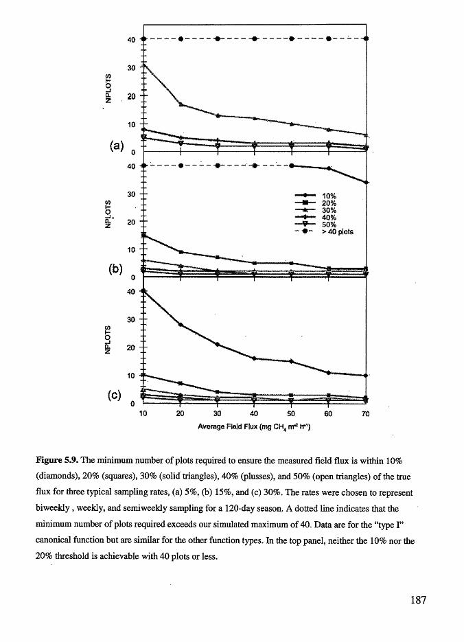
40 -~--·-----------------·----·--~-
30
~ g a. 20 z
10
{a) 0
40 :...---·- _.::.. _ ..... ---·--- --·- -
30 ...... 10% ti) --- 20% b --- 30%
a:· .............. 40% z 20 --9- 50%
•N ·->40 plots
10
(b) 0
40
30
~ 0 ...J 0. 20 z
10
(c) 0
10 20 30 40 50 60 70
Average Field Flux (mg CH4 m4 h"1)
Figure S.9. The minimum number of plots required to ensure the measured field flux is within 10%
(diamonds), 20% (squares), 30% (solid. triangles), 40% (plusses), and 50% (open triangles) of the true
flux for three typical sampling rates, (a) 5%, (b) 15%, and (c) 30%. The rates were chosen to represent
biweekly, weekly, and semiweekly sampling for a 120-day season. A dotted line indicates that the
minimum number of plots required exceeds our simulated maximum of 40. Data are for the "type I"
canonical function but are similar for the other function types. In the top panel, neither the 10% nor the
20% threshold is achievable with 40 plots or less.
187

5.4.2 Question (2)
Question 2 is addressed in Fig. 5.9 where we give the minimum number of plots
required to ensure that the measured flux is within 10, 20, 30, 40, and 50% of the true
flux for three typical sampling rates (5, 15, 30%). These rates roughly correspond to
sampling intervals of biweekly, weekly, and semiweekly, respectively, for a 120-day
growing season. The dotted line indicates levels that are not achievable within our 90%
probability criterion.
10000 -+- 10%
----- 20% --.-- 30% -+- 40%
1000 --9- 50% (/) Q)
c. E «I
Cl) - 100 0 .... Q) .c E :l z
10
1 10 20 30 40 50 60 70
Average Field Flux (mg CH4
m-2 h-1)
Figure 5.10. Minimum number of samples required to attain the specified accuracy limits. The sample
·size is the number of plots times the sampling rate assuming a 100-day field season. For other season
lengths the number of samples needs to be scaled by the ratio (new season length: 100).
These experiments show the difficulty in reaching the highest accuracy levels at
these modest s~pling rates. In fact, the highest accuracy expected using a small
188

number of plots (P~3) is typical~y 30-40%. Only for those fields with large methane
emissions do we expect the measured flux to be within 20% of the true flux if three or
fewer plots are used.
5.4.3 Question (3)
To answer question 3, we considered the total number of_ measurements required
over the course of the growing season to meet our accuracy standards (Fig. 5.10). The
numbers given in the figure are based on a 100-day field season but are easily modified
to accommodate any season length.
The number of samples required range from 1400 per season to ensure the
measured flux is within 10% of the true flux for the lowest emission fields to only five
samples to meet the 50% mark in the highest emission fields. In general we never need
more than about 20 samples per season to reach the 50% mark for any field flux.
However if we wish to reach the 10% stan~ard, we have to sample more than 200 times.
5.4.4 Question ( 4)
From our results in Fig. 5 .11 we see th~t improvements in the accuracy of the
measured flux decreases rapidly with increasing plot number and sampling rate and in
fact become negligible past a certain sampling intensity. Clearly there is no need to
increase the level of sampling past this point. We quantify the diminishing returns of
increasing the sampling intensity by defining an offset gradient relative to both the
number of plots and sampling rate. The offset gradient (dC/dD) is simply the change in
the offset percentage ( C) divided by the change in sampling rate (D) or number of plots
(P), in which case the offset gradient is dC/dP. It tells us how fast the offset is changing
189

as we increase our sampling. We chose D and P to be three and calculated the
gradients over all grid points for the data in Fig. 5.8. We divided the gradients by two so
that the resultant is the change in the offset percentage per unit increase (either plot
number or sampling rate). These are plotted in Fig. 5.11.
190
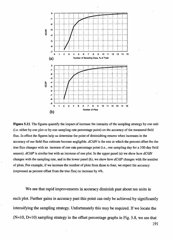
-1
I I I I
-2 ................................... I I I I . . . . . . . . . .
z -3 ..... : ...... ; ..... ~- ....... : ....
s ,, -4 ....... ! ....... ~ ..... -: ........ ·:· ....
I I I I
-5 .... - • ? ..... i .... ·:- .... ·:·.... ~... .. . . . . .......... . . . . . . . . . . . I I I I
..... 1 ...... , •••• J> ................................. . . . . . -6 I I I I
I I I I . . . . . . . . -1 ......_ _________________ _
0 1 2 3 4 5 6 7 8 9 10 11 12 13 14 15
(a) Number of Sampling Days, 9k of Total
I I I I I ~ ....................... .,,, ....... ,. ....... -........... .. . . . . . . . . . . . . . .
-2 .••• ~ .... i· ... -~·. ···:·· ·r ... -~ .... j· ... j·· .. ·~· ... ·( .. ·~· ... ·1· ... i .... ~ ... . -3 .... :· .. ·:··· ··:·. ·:-··· ·:····:····:·· .. :···· :· ... -:···. ·:. ···:· ... :····: ... .
I I I I I I I I I I t I I
I I I I I I I I I f I I I
~ -4 ----~····~---· =·····;·····~---~~----~-- .. ~----·~····-~----·~-----~----~----~ .. --~ .. 5 ..... : .... ~ .... : ...... ~ ..... ~ .... ; ..... : ..... : .. ---~---·..: ...... :. .... :. ..... : ..... : ..... . . . . .
I I I I I
-6 ....... ! .... ~.. .. . ·:· ..... ·:· ..... ~ ...... ~ ....... ~ ...... ~:. ...... ~ .... ·:· .... -~ ..... ~ ..... ~ ........ ~ ...... . . . . . . . . . . . . . .
-7 .... i .... ~ .. ·i· ... -~ .... t .... i .... j .... j .... ~- ... ~- ... ·~ ... -~ .... i .... ~ ... . -8 •.•. ~ ........ ·~· .•. -~- .... ~ •... ~ ... + ... ! .... ·~· ... -~- ... ·~· ... + ... ~ .... ~ ... .
. . . . . . . . . . . . . . . . . . . . . . . . . . . . -9 .....__ _________________ __.
0 1 2 3 4 5 6 1 8 9 10 11 12 13 14 15
(b) Number of Plots
Figure 5.11. The figures quantify the impact of increase the intensity of the sampling strategy by one unit
(i.e. either by one plot or by one sampling rate percentage point) on the accuracy of the measured field
flux. In effect the figures help us determine the point of diminishing returns when increases in the
accuracy of our field flux estimate become negligible. dC/dN is the rate at which the percent offset fro the
. true flux changes with an increase of one rate percentage point (i.e., one sampling day for a 100-day field
season). dC/dP is similar but with an increase of one plot. In the upper panel (a) we show how dC/dN
changes with the sampling rate, and in the lower panel (b ), we show how dC/dP changes with the number
of plots .. For example, if we increase the number of plots from three to four, we expect the accuracy
(expressed as percent offset from the true flux) to increase by 4%.
We see that rapid improvements in accuracy diminish past about ten units in
each plot. Further gains in accuracy past this point can only be·achieved by significantly
intensifying the sampling strategy. Unfortunately this may be required. If we locate the
(N=lO, D=lO) sampling strategy in the offset percentage graphs in Fig. 5.8, we see that
191

this strategy only takes us to within 30-40% of the true flux. In many cases we would
like to achieve a higher standard than this, which will require more flux measurements.
5.4.5 Question (5) Finally for question 5, there i~ a practical limit to the intensity of sampling. A
reasonable limit may be set at twenty plots sampled every other day. This would require
1200 flux measurements over a 120-day growing season. Doing so we find we can get
to within 7 to 14% of the true flux depending on the average field flux.
5.5 Discussion and Conclusions We have examined the observed variability of methane emissions from rice fields
and delineated its components. The nature of this variability affects the accuracy of
regional and global extrapolations and the reliability of field experiments. The
prevailing sampling practices tend to have fairly frequent measurements of about once a
week and more. Because of that, the temporal variability is not likely to be a major
source of uncertainty in the calculated seasonally averaged flux. The spatial variability
however is large, and is not as well handled in the usual sampling strategy by triplicate
plots. A minimum of three plots is convenient and permits statistical comparisons, but
according to our result.s, it leads to large uncertainty in the calculated flux of 40%-60%.
When the flux is low, our calculations show that it takes an unrealistically large number
of replicates to overcome the effects of spatial variability. This is partly because we
have defined accuracy as· a relative measure. Therefore if the true flux is 1 mg m-2 h-1, to
be within 20% we must have a sensitivity of measurement that can distinguish 1 mg
CHi m-2 h-1 from 1.2 mg CH4 m-2 h-1, which is nearly impossible. But for a large flux,
192

say 20 mg CH4 m-2 h-1, to be within 20% requires us to distinguish between 20 and 24
mg Cff4 m-2 h-1, which is possible. 9n the other hand, a great deal of accuracy for low
emitting fields is not needed since such fields do not make a large contribution to the
regional or global emissions. While these statements are true for rice fields, for other
sources such as wetlands, the problem is not so easily dismissed. There are cases where
the flux is low over most of an extensive area. Then the low fluxes are the major
contributors to the regional and global emissions. In such cases chamber methods
looking at small areas are unreliable.
193

Chapter 6-Application of an Empirical Rice Flux Model to National and Global Spatial Scales
6.1 Introduction Rice agriculture is an important source of atmospheric methane but its global
source strength remains uncertain (Denman et al., 2007). In large part this is due to the
many different ways that rice is grown. Neue and Roger (2000) claim that rice is
"cultivated under a wider variety of climatic, so.il, and hydrological conditions than any
other crop", and as a result, methane fluxes range broadly (Wassman et al., 200b; Yan et
al., 2005). Far from being static, these conditions will respond to pressures brought
about by increasing human population, climate change, water shortages, and changing
agricultural practices. Evaluating how emissions respond to these changes is necessary
to predict future forcings of climate and consequent changes.
Emissions from paddy fields are influenced by both natural and anthropogenic
factors, such as climate and the agricultural practices used by the farmer to manage the
field. The practice of intermittently draining paddy fields for example is known to
reduce methane emissions, as is the use of synthetic fertilizers over organic fertilizers.
Considering this, and the fact that methane is twenty times more potent than carbon
dioxide on a per molecule basis, rice agriculture is an attractive source to target for
emissions reduction. This increases the importance of evaluating its source strength
both at the national and global levels. Currently, all countries that are signatories to the
194

United Nations Framework Convention on Climate Change (UNFCCC) are required to
periodically report national inventories of greenhouse gas emissions from all sources,
including rice agriculture. The Intergovernmental Panel on Climate Change has
developed "good practice" guidelines (IPCC, 1997, 2000) for countries to estimate
emissions from these sources based on default seasonal CH4 emission factors and
scaling factors. These IPCC methods will likely be the methods used by countries to
assess reductions in emissions.
Generally, emissions are estimated over-large scales either by upscaling field
measurements or using process-based modeling. As we discussed in the previous
chapter, methane flux from rice agriculture is typically measured using static chambers,
both in the field and in greenhouse studies. Early estimates of global methane emissions
were often based on flux measurements from a single site and tended to be large. For
example, Holzapfel-Pschorn and Seiler ( 1986) used flux measurements from Italy to
derive global emissions of 120 Tg y-1• Using fluxes from multiple sites Khalil and
Shearer (1993) revised this down to 66 Tg i 1• Other studies used a number of proxies
to scale emissions including crop biomass, grain yields, and net primary production.
(Taylor et al., 1990; Neue et al., 1990; Anastasi et al., 1992; Kern et al., 1997).
More recently mechanistic or process-based models have been used to simulate
the dynamics of methane production, oxidation, and emission. Because details of these
processes are largely unknown, in many cases the dynamics of these processes are
linked to other more easily measured variables. For example, Cao et al. ( 1998) related
methane production to soil Eh, and Huang et al. ( 1998) linked the rate of root exudation
195
to the daily aboveground biomass. Others calculated these mechanisms directly. The
Decomposition-Denitrification (DNDC) biogeochemical model captures soil redox
dynamics by simulating soil Eh and the activity of microbial reducers (Li et al., 2002).
Matthews et al. (2000/ presented a model (MERES) that simulates soil organic matter
decomposition and predicts the amount of carbon substrate available for
methanogenesis. It simulates nitrogen transformations in the soil and calculates the
uptake of water and nitrogen by the rice crop.
These mechanistic models are useful in simulating the dynamics and variability
of daily emissions over the duration of the rice growing season for a single site, but both
the data needs and computational expense to apply the models at multiple sites become
prohibitive when applied to global scales. For example, the DNDC model requires
information on soil texture, pH, bulk density, and organic carbon content, besides crop
management properties. Though available at local scales, these details are not known
over wide areas.
Recognizing this difficulty some process models keep the number of input
variables low at the expense of increasing the number of fixed model parameters. A
model described by van Bodegom et al. (2001) requires only eight input variables but
includes about twenty fixed parameters such as root decomposition rate, oxidation rate,
and rice growth rates. Though they are kept constant, there is little knowledge about
how these parameters vary from site to site or during the growing season.
Also some variables that control paddy emissions can change on yearly
timescales, such as fertilization and water management. To investigate the changes
196

these factors make on global emissions requires a model that is deft enough to permit
multi-year simulations. The flux model we used and describe below, allowed us to do
just this and study how known decadal changes to paddy management in China and
elsewhere would translate into changes in the global source strength of methane. We
used this flux model to develop a new global inventory and to investigate possible
changes to the paddy methane budget.
Besides assessments, spatially gridded inventories are useful in other
applications. Spatially resolved inventories provide insight to high emission source
areas at sub-national scales. These regions may be targeted for future study or
mitigation and help focus research efforts. Spatially distributed emissions are necessary
as inputs to regional and global climate models as well as chemical-tracer models.
Patterns of atmospheric concentrations produced by these latter models can themselves
be iJ?.puts to various regional climat~ and chemistry models. This work is becoming
increasingly important as the 1?-eed for planning mitigation and adaptation strategies
around regional climate and impacts increases. Furthermore the patterns of
concentrations predicted by chemical-tracer models can be compared with surface and
remotely-sensed measurements of concentrations to both verify and improve inventories
based on bottom-up techniques. In addition, this forward modeling of surface emissions
helps us to identify the best sites to place instruments in order to monitor emissions and
constrain estimates. Finally, and perhaps most importantly, spatially resolved emission
estimates help us predict the future trend of gas emissions. For example, since paddy
emissions are sensitive to soil inundation which is often achieved through irrigation, we
197

can predict that methane emissions from rice-growing regions of the world that face
future water scarcity, will decrease.
At present few gridded inventories of paddy emissions exist at either national or
global scales. Process models have been applied primarily to country-level emissions,
for example China (Huang et al. 2006; Li et al. 2004) and India (Pathak et al., 2005),
and the few global inventories that exist are based on proxy or statisti~al methods.
Matthews et al. ( 1991) produced a global 1x1 ° inventory of methane from rice
production, but lacking information on how flux varied from site to site, chose instead a
constant flux, such that global emissions were 100 Tg t 1• Bachelet and Neue (1994)
updated this work by scaling methane fluxes to soil type and estimated methane
emissions from Asia are 63 Tg t 1• The most used.global inventory is part of the
Emission Database for Global Atmospheric Research (EDGAR) project. For this
Olivares et al. (2005) used rice ecosystem-based fluxes from Neue ( 1997) and scaled
them by national harvested rice areas from FAO (2000 ). Though an improvement over
single flux methods, only four different flux values were used with no consideration of
the influence of climate or fert~lizer among other factors that control methane flux.
Perhaps the most detailed inventory to date is by Yan et al. (2009 ). Here the authors
used the United Nations Framework on Climate Change Convention (UNFCCC) Tier 2
method to estimate fluxes. The Tier 2 method specifies a base methane flux appropriate
for continuously-flooded fields with no fertilizer inputs. The base flux is then scaled by
designated factors for fields under different management. This inventory estimated
global emissions at 25.6 Tg t 1•
198

Emissions from these inventories have not yet converged at either national or global
levels, indicating a need for continued study and refinement. Our effort sought to move
us closer to this goal by using novel methods and data sets, including the following
innovations.
First, the new inventory is based on a model that is empirically derived from
controlled experiments in a greenhouse and confirmed by measurements in the field.
Though the model is simple in structure, it is complete in the sense it includes the major
variables that control methane from the paddy environment, namely organic carbon and
nitrogen inputs, water management of the paddy, and climate factors. Though more
detailed models exist that adequately predict paddy fluxes they require input that is
difficult to gather at the appropriate spatial and temporal scales. The current model
determines flux base~ on variables that can reasonably be acquired.
Secondly, we used orbital remote-sensing of vegetation to estimate application rates
of crop biomass to paddy fields, a major source of organic-carbon material and driver of.
methane flux. This method provides global coverage of this factor at high spatial
resolution.
Finally, our model includes the impact of nitrogen fertilizer on methane emissions.
Our experimental results indicate that increased rates of nitrogen application increased
methane emissions in paddies continuously flooded but decreased methane emissions
otherwise. To our knowledge, the sensitivity of methane to N-fertilization has not been
included in any other methane inventory.
199

6.2 PSU-Rice Emissions Model Our model is based on a three-year study of methane flux from rice paddies in
Nanjing, China, and experimental pots in the PSU greenhouse during the years 2005 -
2007 (Khalil et al., unpublished). At both sites, the major factors that determine flux
were controlled at various levels and the response of the methane flux measured. The
factors investigated included soil type (sandy loam and silt loam), water management
(continuously flooded, intermittently flooded, and drainage interval), organic carbon
application rate (crop residues), nitrogen fertilizer application rate (urea), and soil
temperature. In China, rice was grown in adjacent plots that measured 4 m x 4 m, while
in the PSU greenhouse, rice was grown in microcosms that had footprints of 45 cm x 63
cm. At both sites, methane and nitrous oxide fluxes were measured by the rate of
accumulation in static chambers placed over the rice plants. A summary of results from
both the greenhouse and field site is shown in Fig. 6.1 for seventeen experimental
conditions.
The figure shows that there is good agreement between the fluxes measured from
the greenhouse and the Nanjing plots, which gives us confidence that the relations
between flux and factor developed from all these data are robust and may be applied to
other sites. All relations are based on evaluation of the seasonally averaged flux. We
summarize these relations as follows.
200

Figure 6.-1. Methane fluxes from greenhouse (red) and field (green) studies. Fluxes are plotted against
different factors and levels of factors. Key to numbers: The experiments are classified by water
management (W), organic carbon inputs (S=straw), and nitrogen fertilization (N). WO=continuous
flooding, W2=intermittent flooding, Sx = Straw added, where x=O, 1,2,3 and depends on application rate
(0, 3, 6, and 9 Gt dry matter ha-1, respectively). Nx= nitrogen fertilizer where x=O,l,2,3 depending on
level (0, 100, 220, and 300 kg N ha-1, respectively). The last three experiments are for midseason drainage
conditions Dx, where x=l,2,3 showing increasing drainage (5, 10, and 15 days, respectively).
l=WOSONO, 2:;:::W2SONO, 3=WOS1NO, 4=WOS2NO, 5=WOS3NO, 6=W2S1NO, 7=W2S3NO, 9=W2SON1,
lO=WOSONl, 1l=WOSON3,12=W2SON2, 13=W2SON3, 15=WOS2Nl, 16=W2S2Nl, 17=WOSIN2Sl,
18=WOSIN2SO, 19=WOS1N2 (no plant), 20=W2SIN2Dl, 21=W2SlN2D2, 22=W2S1N2D3. From
Khalil et al. (unpublished).
Methane flux increased when increasing supplies of organic carbon was added to
· the soil (experiments 3-5 in Fig. 6.1). At both sites, the organic carbon was supplied by
the addition of rice straw. Methane flux decreased when sites were managed under an
intermittent flooding regime, i.e. fields were drained at least once during the season
{experiments 6-7). The addition of synthetic urea decreased the methane flux
(experiments 15-19), while methane flux also decreased as the drainage period
increased (experiments 20-22). From ~hese measurements the following relation was
developed (Khalil et al., unpublished)
201

(6.1)
Here Fis the methane flux in units of mg CH4 m-2 h-1, F0 is the base flux with no
organic carbon or nitrogen fertilizer application, C and N are the amounts of added
organic carbon and nitrogen fertilizer with units of g (dry biomass) m-2 and g N m-2,
respectively, a is the sensitivity of the flux to the added organic carbon, and f3 is the
sensitivity to nitrogen fertilizers. F0 = 7.3±2.7 and 2.4 ±0.8 mg CH4 h-1 m-2, and/3
=0.016 and-0.036, for continuously and intermittently flooded fields respectively. The
experiments showed that a is temperature dependent according to
(6.2)
where ao = 0.021, p1 = -0.0021, p2 = 0.0000551, and Tis the average soil temperature
(at 10 cm depth) in degrees Celsius over the first 60 days of the season (described
below).
The rates of nitrogen fertilizer _and organic carbon application varied by a factor
of three in the study, while temperatures spanned the range over which most rice is
grown, ensuring the model will have wide. The next step was to apply the model to
national and global rice agriculture and create a spatially gridded inventory of methane
emissions.
202

6.3 Model inputs
Regional and global extrapolation of the empirical flux model developed from the
field and greenhouse studies required spatially resolved clim3:te and agriculture data.
While some of these data are readily available, others such as organic carbon and
synthetic fertilizer application rates are available only over limited areas and spatial
resolutions. Data such as water management and crop residues, which are often
incorporated back into the paddy, do not exist in any official form. Properly
representing the field conditions and paddy management over national and global scales
remains one of the primary sources of uncertainty in estimates.
203

+5N
+oN
J5N
JON
·Q. ~·
20N .;Tl"' ·"-.tl!lliiO"_ '
15N
10N
5N
. "' {t· ~ ... ,,, · ~ -,. .. ;. ' ~-
\ "~ j ~~.· .. i ~-Y
EQ
SS
105
6 E 7 f
100 300 500 700 900 1100 1300
Figure 6.2. Harvested area of rice agriculture in units of hectares per cell. Harvested area is the area of
rice harvested per year. For multiple croppings of rice, the harvested area will exceed the physical area.
Harvested data are from Monfreda et al. (2008) . Resolution of map is 5 arcmin.
We constructed underlying data layers as model input for the following factors:
rice location and area, crop calendar (i.e. planting and harvesting dates), soil
temperature, organic carbon and nitrogen inputs, and water management (inundation).
A brief description of each follows.
204

6.3.1 Location and extent o~rice growing areas Rice growing locations and areas are taken from Monfreda et al. (2008) and
shown for monsoon Asian countries in Fig. 6.2. The authors distributed statistical
national and subnational rice cropping areas on a 5 arcmin x 5 arcmin ( -10 km x 10 km
at the equator) grid based on a global cropland base map (Ramankutty et al., 2008). The
base cropland product provided fraction of pixel area that is determined by two sources
of satellite land cover data. The data provided are harvested areas, which may be larger
than actual land area if more than a single crop is ha.rVested seasonally on a single
parcel of land. The total area of harvested rice from this product is 152 million ha.
6.3.2 Crop phenology The timing and duration of rice seasons is needed not just to calculate annual
emissions from a flux, but as we describe below this information is also used to estimate
appropriate soil temperatures and straw inputs to the paddy field. Crop phenology is
complicated by the practice of multiple cropping seasons in a single year. Though some
rice growing regions may only have a single rice crop due to climate limitations or
economic preferences for alternate non-rice crops, other areas practice double or triple
rice crops in a single year. A typical rice season in the tropics may be 100 days but 130
days in temperate regions.
We used rice crop calendars developed by Matthews et al. ( 1991) for this study.
Matthews et al. (1991) compiled rice crop calendars from the United Nation's Food and
· Agriculture Organization (FAO, 1978), the International Rice Research Institute's
World Rice Statistics (IRRI, 1985), and other national and subnational agricultural
statistical handbooks and atlases (see Appendix of Matthews et al., 1991 for complete
205

list) and distributed them across a lxl 0 global grid. A total of 36 different crop cycles
were included in the data base including single, double, and triple cropped rice. The
· number of months per year rice is grown ranged from 4 to 12. Crop calendars were
available at the national level for most countries, but for China and India, calendars
were provided at the provincial and state levels. Since the resolution of our inventory (5
arcmin) is higher than the crop calendar grid (1 deg.), we took the calendar to be
constant throughout the one deg. grid cell. Also, in those rice-growing regions where no
cropping information was provided by the Matthews et al. map, we use a nearest
neighbor algorithm to assign appropriate cropping data.
As rice-cropping management is based on climatic, ecological, and cultural
factors, as well as individual decisions made by the farmer, large differences in planting
and harvest dates, crop duratio.n, and number of crops per year, exist. In addition,
multiple cropping may occur on a regional scale but not necessarily at the individual
field level. While there may be early, intermediate, and late season rice crops within a
region, a single field may only be planted for one of these seasons, while others in the
same region may be planted for two or all of the seasons. The agricultural statistical
data needed to delineate these differences in rice cropping were unavailable at this level
and we recognize this as a source of uncertainty in the final inventories.
6.3.3 Soil temperature
From our flux measurements we determined the sensitivity of both methane and
nitrous oxide flux to soil temperatures. The data indicate that temperature is an
important driver of methane flux, but less so for nitrous oxide. In our empirical flux
206

30
25
20 0
g> 15 "C ...,:
10 • ·5 en
5 •
0
-5
• •
• •
5 10
•
15 20
Daily surface T, deg C
y = 0.85x + 3.6
R2 = 0.92
25
Figure 6.3. Surface ~d soil temperature at Tuzu, Sichuan Province, China (2005-2006). Soil
temperatures were measured at a depth of 5 cm.
30
model, the parameters a and ~ are the sensitivity factors that relate both CH4 and N20
fluxes to organic carbon and nitrogen inputs respectively. Our experiments revealed that
a is a strong function of soil temperature, while ~ shows no significant dependence on
soil temperature.
Soil temperatures were derived from reanalysis surface air temperature from the
National Weather Service's National Center for Environmental Prediction. Surface air
temperature data are distributed globally on a 2.5x2.5° grid at a daily time scale. Daily
temperatures from the years 1948 to 2006 were averaged to produce a climatological
record for use in deriving the soil temperature data.
From the greenhouse and field measurements of methane flux, the functional
relationship between a and T was statistically stronger using the average soil
207

temperature over the 60-day period following rice planting rather than over the entire
rice season. To this end, the beginning of the rice season was determined separately for
each grid cell based upon the crop calendars described above. Daily air temperatures
were averaged over the 60-day period following this date. After the daily averaging was
performed, surface air temperatures were converted to soil temperatures (at approximate
depth of 10 cm) using a linear relationship derived from two years of soil/air
temperature data from field measurements in Tuzu, China (Fig. 6.3). The map of soil
temperatures is shown in Fig. 6.4.
SON
JON
[Q
. ; . · · ·.~; : . ·: .... ..... .
30S .
14 16 18 20 22 24 26 28 .30
Figure 6.4. Soil temperatures at 10 cm depth averaged over the first 60 days of the growing season.
Temperatures are notably higher in the Indian sub-continent producing larger fluxes in paddy fields .
208

6.3.4 Organic carbon inputs Both greenhouse and field experiments clearly sho~ the strong dependence of
CH4 fluxes on organic carbon inputs. In these experiments organic carbon was added to
paddy soils in the form of straw. Ill practice, organic carbon can be added in myriad
ways.
To simulate the addition of organic carbon to paddy fields in our model we
considered the largest sources of organic carbon, including straw, crop roots, stubble,
and farm manure. It is common practice to add rice straw and other residues back to the
field after harvest (Neue et al., 1996,· Wassman et al., 1996). These organic amendments
are an important source of fermentable carbon for soil methanogens (Wassman et al.,
1996) and increase methane emissions. Methanogens utilize the labile carbon
preferentially leaving the cellulosic materials behind (Yagi and Minami, 1990, Cao et
al., 1995, van Bodegom et al., 2001). As this labile carbon has a short residence time in
the soil, perhaps one to two months under the right soil and environmental conditions
(van Bodegom et al., 2001), only the organic matter received by the paddy soils within a
couple :111onths of rice planting· will stimulate methane emissions.
The application rate of crop residues depends on the crop standing biomass and
the fraction of residue returned. In some cases the residue is burned, used for energy, or
used in straw products (Wassman et al., 2000). The crop biomass production is variable
and depends on factors such as rice cultivar, length of growing season, water stress, and
C02 levels (Summers et al., 2003; Cheng et al., 2008). This variability adds uncertainty
to estimates of methane emissions across large areas. Though ·some survey data exist
from Chinese farmers quantifying this input (Huang et al., 2006) in genera~ there is very
209

little information about the amount of straw and residues added to paddy fields. To our
knowledge none exists on a gridded basis.
Remote sensing data can help fill in these gaps. Surface reflectance
measurements from space have been used over the past decades to construct land use
and land cover maps, and to estimate biophysical parameters from vegetation (cf.
Mather, 1993; Alexander and Millington, 2001; Liang, 2004). Of particular interest for
this study is the use of satellite products to infer biophysical parameters from crop
agriculture (Tan et al., .2005, Zhang et al., 2005; Zhang et al., 2006). Remote sensing
has been shown to provide accurate assessments of crop growth, production, and area,
and yield (Tucker et al., 1980, Sharman et al., 1992; Moulin et al., 1998). For example,
crop monitoring by space provided better estimates of U.S. Com Belt crop yields during
the 2005 droughts than standard methods (Zhang et al., 2006).
210

1.2 - - - - - - - - ·- - - - - - - - - - -- - - - - -
(a) 1 -------- -----·------------
1 0.8 - - - - - - - - - - -- - - - - - - - - - -· -
i .!::! 0.6 1ii E ;; 0.4 z
0.2
0 0.3 0.6 0.9 1.2 1.5 1.8 2.1 2.4 2.7 3
MOD15 LAI
Broadleaf Crops
Broad leaf Forests
ll")
~ ...... >< rl.:I
~ ·s.
Vl
Needleleaf § Forests ><
r.IJ Gl >< ·a.
18
12
6
0 12
9
6
3
0 0 1 2 3 4 s 6 7
LAI
Figure 6.5. Distribution of leaf area index (LAI) for (a) modeled rice agriculture lands, and (b) other
vegetation types. Solid line in (b) is from the MO DIS Collection 4 product, while dotted line is from
Coll~tion 3. LAls in plot (a) range up to about 3 with a median value of 0.92. This is similar to the
general distribution of LAI observed for all broadleaf crops seen in (b) confirming that MOD15 LAI is
correctly picking out croplands. Figure (b) from Shabonov et al. (2004 ).
We used crop leaf area index to estimate standing biomass in rice growing
region~. The leaf area index (LAI) is the ratio of the total one-sided leaf area to the area
of the footprint the plant projects. It can be as high as seven for dense forest canopies
(e.g. Shabonov et al., 2005), but is typically 1to1.5 for croplands and rarely exceeds
three (Shabonov et al., 2005; Tan et al., 2005) (Fig. 6.5). Leaf area index products are
calculated from satellite observations by optimizing the match between measured and
modeled surface reflectances. Simulated reflectances are calculated using a radiative
211

transfer model that considers variables such as soil reflectance, leaf reflectance, and
canopy transmittance for a number of vegetation categories (Myneni et al., 1997; Liang
2004). The vegetation categories are supplied by a land cover map.
We used the Collection 5 MOD15 LAI products at 1 km resolution (Myneni et
al., 1997, Myneni et al., 2002) for the year 2001. This product has been validated
against ground measurements and compared against other satellite derived LAI
retrievals (Garrigues et al., 2008). In general it reproduces the seasonal variability of
cropland vegetation well, and among the four LAI products tested in Garrigues et al.
(2008), it most accurately reproduced the ground measurements. However, the MOD15
LAI tends to underestimate cropland LAI (Garrigues et al., 2008) and we scale all
MOD 15 LAI by a factor of 1.4 to correct for this.
Though the MOD15 product is available every eight days, we used monthly
averages since our crop phenology is specified at monthly timescales. For each grid cell
with harvested paddy area, we determined the beginning month of each rice season
based on the crop calendar described above. For the two months preceding this date we
determined maximum LAI for the grid cell using the MOD 15 product. Again our
assumption is that residues from the crop preceding rice planting will be added to the
paddy field the following season. We used a time frame of two months to account for a
possible transition month between crops. We used the maximum LAI over this period,
rather than the mean since LAI may go to zero after harvest and perturb the mean.
212

18000 ._ ------------------··----------- ·--- --· ·----·····-- •.
16000 - • - - - • - - • - - - - ••... - - - - .. - ... - . - • - .•. - - . - - . - .•. - - - - - .
14000 - - ••• - - - • - - .. - - - - - . - - •.. - - - - - - - . -- - - . - - - . - - - - - - - - -
12000 ---- l -----: DPllrlC
t 10000 -~··· !-··--.: !
- - · · - - • .. • • • • - ·· • • ·· · • • ·· .. • · • · - - - ·· • • ~ • • • ITotilC
·a, 8000 . -- I
: : :: : ! 2000 ·---- l
0
:
i o ~ ro ~ ~. ~ ~ ~ ~ ~ ~
appl~C {gCJm2)
Figure 6.6. Simulated organic amendement application rates from all model grid cells with harvested rice
areas. Contributions from crop residues (PlantC) and farm manure (ManureC) is shown along with the
combined rate (TotalC). Values are in the range, but on the low end, of rates reported from actual farm
practice.
Though there is vanability between .vegetation types, overall there is a good
relation between LAI and aboveground biomass (e.g. Baccini et al., 2008; Xioasong et
al, 2008). For rice and related crops at maximum height, the ratio between aboveground
mass and LAI is about 310 ± 20 (Xiaosong et al., 2008) and we scaled all LAis by this
ratio to determine biomass production.
After grain harvest, the aboveground biomass is the sum of straw ~d stubble.
The mass of crop stubble is about 13% the mass of the straw (Huang et al., 2006), so
the aboveground biomass is 1.13xstraw. The mass of crop roots is about 10% the mass
of the abov~ground biomass (Huang et al., 2006). If the roots and stubble are
incorporated back into the field as standard practice shows (Huang et al., 2006) and
213

/'
50N _ .... :
r 550
40N 500 .. 450
JON 400 , ... . ,
350 ... 20N
300
250 .. I 200
10N , , 150 .... ·'. f ·, .. 100 EQ . . ., . :. .. ~ . .-,..., 50
• "" · \ .. 4 .. ..,, • __ ., 105
60E 70E 80E 90E 10DE 110E 120[ 130E HOE 150[
Figure 6.7. Simulated organic amendment application rates for rice producing regions of monsoon Asia.
Units are g (dry matter) m-2_ Values include contributions from both crop residues and organic manure.
The rates range from 15 to 1020 g (dry matter) m·2, with a median of253 g (dry matter) m-2•
some fraction/ of the straw is added to the field, then the organic matter amendment
from the previous crop is given by:
crop residue application= AGB x (o.i f +O. l3) (6
_3)
1.13
214

where AGB is the aboveground biomass (g m-2). For China, the fraction of straw added
to the paddy field varies between 5 and 30% by province according to farmer (Huang et
al., 2006). Outside China the average fraction is 15%.
Animal manure is sometimes added to rice paddies and increases carbon
substrates in rice paddies. Farm animal manure remains the primary fertilizer in some
rice producing countries, but is being replaced by mineral N fertilizers elsewhere. The
amount of manure applied to paddy fields is uncertain globally, but good estimates exist
for China from agricultural surveys. Reported inputs are available by province and
range from 6 to ~00 g C m-2• Elsewhere we estimate application rates based on farm
animal populations (F AO, 2005) and country-based manure production per head of
animal (Mosier et al., 1998). Dry manure values were converted to carbon using carbon
fractions from Bustamante et al. (2008 ).
Our estimated total organic matter application rates are shown in Fig. 6.7. Rates
ranged from 15 to 1020 g (dry matter) m-2, with a median of 253 g (dry matter) m-2
. bur
simulated rates peak around 120 g C m-2• If we assume a carbon fraction 0.4 for dry
biomass, this rate translates into an application rate of 3 t ha-1• This value is consistent
with actual farm practices, though on the low end of reported values (Neue et al., 1996;
Khalil et al., 1998).
6.3.5 Nitrogen inputs Nitrogen fertilizer inputs affect not only nitrous oxide emissions but methane
emissions as well, though the relation is more complex for methane. Our measurements
indicated that under continuously flooded conditions, methane paddy flux increased
215

with increasing nitrogen additions; however, under intermittently flooded conditions the
relation is reversed as the methane flux decreased with increasing nitrog~n inputs.
Nitrogen application rates are determined from two sources. The FertiStat
database of PAO includes rates of N fertilizer applied to rice paddies (kg N ha-1) for all
countries over the years 1995 - 2003 (http://faostat.fao.org). In addition, the FAQ
FertiStat data includes the percentage of rice paddy area fertilized in each country. Only
for this fraction of paddy area do we apply the specified fertilizer rate. For the
remaining area set the application rate to zero.
For China, we used total N fertilizer application rates (for all crops) at the
county level (EOS_Webster, http://eos-webster.sr.unh.edu/home.jsp). We scaled these
totals by the fraction of total cropland that is rice paddy area at the county level and grid
appropriately.
6.3.6 Inundation Our flux model differentiates paddy fields that are managed under continuously
flooded regimes versus those that are intermittently flooded throughout the rice season
since fluxes are significantly different between the two. For example, CRi flux was
approximately three times higher in the continuously flooded control plots (no organic
carbon or N-fertilizer additions) than in the intermittently flooded plots (7.3±2.7 vs.
Yan et.al. (2009) used statistical databases from the FAQ (http://faostat.fao.org)
and the International Rice Research Institute
(http://www.irri.org/science/ricestat/pdfs/Table%2030.pdf) and rice maps from Huke
216

and Huke (1997) to compile proportions of paddy areas in each country that were ;
managed under continuously flooded, intermittently flooded with single drainage, and
intermittently flooded with multiple drainages. Outside of Vietnam where nearly all
paddies are continuously flooded, the typical proportion of paddies that are
continuously flooded is 20-30%. In China, roughly 80% of paddy fields are
intermittently flooded with multiple drainages. A greater proportion of paddy area in
India is continuously flooded (30% vs. 20% ), and the remainder area is roughly evenly
split between single and multiple drainages. These country proportions are implemented
in our gridded inventories by calculating averages of fluxes for each water regime
weighted by the country-specific area proportions.
217

:z Cl
"'
~·
\ ,
..... 0 ,..,
C>
Figure 6.8. Simulated seasonally averaged methane fluxes across all rice-producing areas. Units
are mg C~ m-2 h-1• Grid cells are 5x5 arcmin. For grid cells that contain fields that are multiply
cropped, fluxes displayed are averages across seasons.
218

6.4 Methane fluxes and emissions We created gridded maps at 5 min x 5 min resolution for each of the above input
variables. Using the functional relations in our model that were derived from the field
I
and greenhouse work, we calculated the seasonally averaged flux for each grid cell and
crop season (Fig. 6.8). As some fields have three crops per year, the fluxes shown are
averages over all seasons if the crop calendar for the grid cell indicated that fields
within the cell were multiply cropped. Over the course of the simulated year, over
719 ,000 fluxes are calculated for all grid cells and seasons. Simulated fluxes ranged
from 3.1 to 170 mg CH4 m-2 h-1, though as Fig. 6.8 shows, most fluxes are within the
lower part of this range. This is consistent with the range of 3000 fluxes from measured
from paddy fields in China (1 - 180 nig C~ m-2 h-1) reported by Khalil and Rasmussen
( 1991 ). van Bodegom et al. (2000) also estimated that seasonally averaged fluxes across
China, the Philippines, and Indonesia vary by two orders of magnitude using a process-
based model for rice paddy emissions.
Our area-weighted mean flux over all countries and seasons is 6.6 ± 2.3 mg C~
m-2 h-1. Thi~ compares well with the base emission factor of 5.4 mg CH4 m-2 h-1
recommended in the 2006 IPCC Guidelines for National Greenhouse Gas Inventories
(Yan et al., 2005; IPCC, 2007). The baseline factor is for continuously flooded fields
with no organic amendments. Our average flux includes contributions from fields that
are both intermittently-flooded and those that receive organic amendments. Since these
two factors drive fluxes in opposite directions, we can expect our average flux to be
close to the baseline emission factor. Our mean flux is also typical of values measured
from European and American rice fields. Published fluxes from Spanish, Italian, and
219
Californian rice fields range from 4-16 mg C~ m-2 h-1 (Cicerone and Shetter, 1981;
Seiler et al., 1984, Holzapfel-Pschorn and Seiler, 1986; Schutz et al., 1989). This
suggests that our model is simulating fluxes reasonably well worldwide.
The spatial distribution of fluxes in Fig. 6.8 shows some new and interesting
results. Fluxes in China are generally lower than in other monsoon Asian countries. In
particular we see "hot spots" of flux along the India/Pakistan border, near the coastal
regions of southeastern India, and in Vietnam. Fluxes are lower in China mainly for two
reasons. First, average soil temperatures here are lower than in lower latitude countries,
but secondly, much of the paddy fields in China are drained at least once throughout the
season. It is estimated that only 20% of paddy fields in China are continuously flooded
(Li et al., 2,002). The fraction of fields that are continuously flooded is higher in most
other Asian countries. In Vietnam, nearly all paddies are continuously flooded and this
leads to an average flux in Vietnam of 19 mg CILi m-2 h-1, which is about 3.5 times
higher than China's average flux.
220

55N
50N ...
-4-5N 400
+ON 360
J5N 320
JON ·"- 280 .,
25N ·fl ~. 240
20N \
. 1\ 200
15N 160 . 10N 120
5N
·rfj~·,_ 80
EQ 40 0 • Cl~.
SS . ·. ...a - ' . .; 105 ~-··
60E 70E BOE 90E 100E 110E 120E 130E HOE 1SOE
Figure 6.9. Methane emissions from south and southeast Asia paddy fields. Units are metric tons CJL i 1•
Emissions were calculated by integrating fluxes over growing seasons and
harvested areas of each grid cell. Emissions from multiply cropped fields were summed
for annual totals. Gridded emissions are displayed in Fig. 6.9 for monsoon Asia and
national sums for select countries are given in Fig. 6.10.
We estimated that the annual emission from rice paddies globally is 49 ± 18 Tg
CH4 y' 1• This lies towards the low end of the historical range of estimates, but is roughly
in the middle of more recent estimates (Fig. 6.11 ). Over time, estimates of global
emissions have generally decreased. In part, this is due to the limited number of fluxes
221

from which early estimates were calculated. Fluxes were seldom measured over an
entire growing season, or if they were, they were measured only from a single field
under one set of conditions. For example, the first published global estimate of 190 Tg
y-1 (Koyama, 1963) was based on laboratory incubation ~f paddy soils. Schutz et al.
( 1989) extrapolated the flux from a single Italian rice field to estimate global emissions
of 100 Tg y-1• Early studies also used a rice-growing season length of 140 - 150 days,
based upon growing seasons in California where many of the early measurements were
made (Cicerone and Shetter, 1981; Seiler et al., 1983). Growing season length is quite
variable worldwide, and in the tropics may be only 77 days (Matthews et al., 1991).
222

10 ...... -
0 to to (') (') :J :l c... :::s\ r s:: z -0 -0 -{ < S» c: Q) ::r c. c. Q) 0 Q) Q) CD Q) 2: ::r (i)" :J """ 3 5· i»" 0 "C """ 0 '<"° "C " ~- ...... co 3 :l
Q) CD en ~ Ci)" -a· i»'" :J
i»'" Q) O" Q) - CD :J .?> Q) ...... "C Q) 0 x en Q) . :J 3 c. c. 0 en Cf) i»" :J :;· c.
CD i»" bi i»" CD en en ::r -Figure 6.10. Annual emissions from rice agriculture for select countries of monsoon Asia.
- With more studies, it became ~apparent that C~ fluxes varied widely over fields
where rice was grown under different ecosystems and conditions. This led to a revision
downward of estimates. Recognizing this, Neue et al. ( 1990) reduced the estimated
range of emissions to 25 - 60 Tg i 1• More recently Yan et al. (2009) estimated global
emissions to be 26 Tg C~ y-1 using the 2006 IPCC Guidelines (IPCC, 2007). This is
somewhat lower than our estimate. Though it is difficult to determine the exact cause
for the difference, it likely has to do with temperature effects. There are no temperature
scaling factors in the IPCC Guidelines, meaning there is no variation of flux with
temperature throughout the rice-growing regions, despite an abundance of observational
and experimental evidence that shows temperature is important (e.g. Seiler et al., 1984;
223

Holzapfel-Pschom and Seiler, 1986, Khalil and Rasmussen, 1991; Khalil et al., 1998).
Fluxes in our model are sensitive to temperature (Q10 = 3.7) and are significantly higher
~an the IPCC baseline emission in regions where the seasonally averaged temperature
is higher than about 25°C. This causes the integrated einissions over these regions to be
much higher than the estimates of Yan et al. (2009 ). We discuss the temperature effect
further below.
Though rice is grown globally as seen in Fig. 6.8, most emissions are from south
and southeast Asia where rice is a staple crop and provides a large percentage of the
daily calories. We estimate that this region is responsible for about 90% of the world's
emissions, with major contributions from India, China, Vietnam, and Bangladesh along
major rivers and deltas (Fig. 6.10).
224

'r""
200
180
·~ 160 O>
t- 140 ~ :::c
0 120
~ 100 "'C
~ 80 0. cu 60
..0 0 40
C!J 20
•
. f I •
0 +-~.----.~-.-~-.--~.-~,----,-~--,-~-.--~-,--~.--,-~---r-~-,-----, --1 ~ =ij -< en z "1J en =ij tIJ en :c en 0 ;::s;; :::r ll> :::r CD ll> 0 0 0 ~- c=;· 0 c;r ::::s 0 ::::s CD c: 0 en 0 c: :::r N" a> CD '< () CD ll> CD () en () 3 c: ll> -c ll> :e m. "1" -c 3 r+ -c
ll> - - - ll> "C 0 0 1\5 CD -L ~ ::::s
~ ~ -c ::::s -L -L ::::s - - ll> -c 0 (0 (0 (0 -L CD CD
""' ll> a. (0 - I ~ -I\) 0
1\5 ::::s (0
~ (0 -L (0
"1J ll> -L
..:::! a. en ~ 0 (0 (0 ::::s (0 0 0 ll> - (0 .9 en -L a. CJ) 0 0 ;::s;; en .9
0 (0 ~ $ U> :::r en :::r CX> en - ~ - 0 ~ :::r
-L -c CD (0 ::::s :=a:
1\S (0 ll> CD $ ::::s -c 0 a. -0 en -L
.9 (0
~- CX> a> -L
-c --L
(0 CX> ~
Figure 6.11. Published estimates of global CH. emissions from rice agriculture.
Noteworthy is the distribution of emissions between countries within this region.
We estimate emissions from China to be 5.1±1.8 Tg i 1• This is considerably smaller
than an early estimate of 30 Tg i 1 (Khalil and Rasmussen, 1991), but is consistent with
more recent work. Yan et al. (2009) and Huang et al. (2006) estimated emissions from
China to be 7.4 Tg y-1 and 6.0 Tg i 1, respectively. National emissions reported by the
225

Chinese government to the UN Framework Convention on Climate Change were 6.1 Tg
i 1 in1994 (UNFCCC, 2000). Chinese paddy emissions in the popular
EDGAR3.0FT2000 data set (Emission Database for Global Atmospheric Research,
Olivier et al., 2005) are over t~vice as large (13.7 Tg i 1). The EDGAR inventory uses
an emission factor of 340 kg CRi ha-1 for China based upon a report by Neue ( 1997 ). If
we assume a season length of 120 days, this translates into a flux of about 12 mg CRi
m-2 h-1, which is about double our value. The discrepancy arises because the reported
emission factor in Neue ( 1997) is for irrigated fields only, which in general have higher
fluxes that rainfed or deepwater rice (Neue, 1997; Wassman et al., 2000). With full
accounting of all rice ecosystems, national emissions of 5 - 7 Tg y-1 are more
reasonable.
While China is commonly considered the world's largest source of paddy CRi,
we estimate that India has significantly higher emissions than China (Fig. 6.10). In part,
the misconception stems from a report by Mitra ( 1992 ), wherein the author reported that
total paddy emissions in India totaled only 3 Tg y-1• This surprisingly low total was due
to a nearly zero emission rate measured from India's irrigated rice fields, which make
up about 45% of India's total harvested area. It was later revealed that the low fluxes
were measured from fields that had high percolation rates, and were flooded for perhaps
only 1-2 days per week (Neue, 1997).
Our estimate of emission for India is 15 ± 5 Tg i 1• This is higher than the
estimate of 6 Tg i 1 and 9 Tg i 1 by Yan et al. (2009) and Olivier et al. (2005),
respectively. National emission of 4.1 Tg i 1 was reported by India to the UNFCCC in
226

1994 (UNFCCC, 2000). These however were based on measurements by Mitra (1992)
and are presumably underestimated for reasons given above. Olivier et al. (2005) used a
global default emission factor for India's irrigated rice fields, due to confusion with the
Mitra ( 1992) data set. The default value is lower than all other national emission factors
in monsoon Asian countries, except the Philippines. For reasons related to temperature
described below, this is unlikely. Therefore the EDGAR value is likely underestimated.
Our findings are consistent with known changes to rice management that have
occurred in China over the past couple decades In.the early 1980s Chinese farmers
realized that intermittent draining of their rice fields midway through the rice season
increased grain yields (Neue, 1997; ii et al., 2002). As a result, only about 20% of
paddy fields are now left flooded throughout the season (Yan et al., 2009)~ which
dramatically lowers methane fluxes. Li et al. (2002) estimated that C~ emissions from
Chinese paddies decreased by about 5 Tg i 1• since the early 1980s. Our results support
this reduction in emissions as we discuss in the next chapter.
Besides these differences, Chinese emissions are also smaller due to lower
seasonally averaged temperatures. Our experimental results showed that methane
emissions respond strongly to temperature, and this is refle~ted in the flux model. The
area-weighted seasonally-averaged soil temperature is 21.3°C, and 24.5°C for India.
The baseline emission factor used by Yan et al. (2009) does not account for
temperature, and produces low emissions. China also has a larger .fraction ( .... 30%) of its
total harvested rice area planted in the early spring when temperatures are cooler than
India (<5 %) (Matthews et al. 1991).
227

One final consideration is the use of mineral N-fertilizer. Our experimental work
showed that the addition of N-fertilizer enhanced Cl4 flux in continuously flooded
fields but reduced the flux in intermittently flooded paddies. Globally, N-fertilization
has little impact on emissions; however, at the country level it does. In China, N
fertilization decreased emissions by 0.6 Tg Cf4 f 1, while in Vietnam it increased
emissions by 1 Tg CI4 f 1. The difference is due to the larger fraction of continuously
flooded paddy area in Vietnam.
One final noteworthy result is the relatively large emissions from Vietnam (6.3 Tg
f 1), which puts it on par with China, despite China having over four times more
harvested area than Vietnam. Again this result is due to water ma1:1agement. It is
believed that all of Vietnam's paddies are managed as continuously flooded, making it
unique among Asian countries (Yan et al., 2009). If we set the water management of
Vietnam equal to that of China, Vietnam's emissions would be halved. We again see the
importance of water management on rice pa~dies, and. quantifying this factor accurately
across all rice growing countries would be a major contribution to the methane budget.
We are investigating the use of backscattering data from space-borne instruments to
map inundation at high resolution spatial scales.
If methane emissions are about 50 Tg y-1 as we suggest, rice agriculture is one of
the most important anthropogenic sources of methane. The large range of emissions
reported for other sources makes it impossible to rank rice agriculture unequivocally.
The only anthropogenic source that consistently has emissions ranked higher than 50 Tg
y-1 is ruminants (80 - 100 Tg y-1). This means that rice agriculture makes a significant
228

contribution to atmospheric levels of methane. It is believed that the increase in rice
cultivation 5000 years ago led to the reversal of a natural decline in atmospheric CH4
(Ruddiman et al., 2008). Growth in rice production during the twentieth century added
to the increasing methane burden. Future scenarios of methane emissions must take into
account rice agriculture and how emissions from it may respond to changing drivers.
We take up this challenge in the next chapter.
229

Chapter 7-Trends of Methane Emissions From Rice Fields and Mitigation Potential
7 .1 Introduction Rice agriculture is one of the largest sources of anthropogenic methane and may
be an important source to target for mitigation (Neue et al., 1997; Ding et al., 1999). Its
production has nearly tripled over the past fifty years with a nearly constant 3% annual
growth rate (IRR!, 2010). In parts of the world where rice is grown, changing paddy
management practices have likely led to reduced methane emissions. Quantifying thes.e
changes is difficult however, as the production and release of methane from paddy
fields depends on a large number of spatially and temporally heterogeneous variables
which are poorly quantified over large areas.
In this study we used a novel empirical model derived from multiple years of
greenhouse and fiel~ studies to assess the trends in rice agriculture emissions. We
considered mainly the impact of changes in the use of organic carbon and nitrogen
fertilizers, water management, and temperature to paddy emissions. Our time frame of .
interest was from 1980 to the present when management practices changed
dramatically. Our results indicated significant decreases in methane emissions over this
time. We also considered the future trend of emissions ~ased on expected scenarios, and
assess how much further decrease in methane emissions we could expect under
mitigation strategies.
230

39
37 <D lo...
as 0 35 Q) ..c: c:
.. Q 33· .E -as Q) 31 lo... as Q) CJ ·c:
29 "'C Q) -en Q)
c: 27 as :c
25 1960 1970 1980 1990 2000 2010
Figure 7.1. Harvested hectares of rice in China. Data from the Food and Agriculture Organization (FAO,
2009).
We limited our analysis to China, for which we have reasonable information
regarding changes in water management and fertilizer usage. We explored global
mitigation possibilities by developing scenarios of drivers.
7.2 Changes in drivers We can generically express emissions E(t) (g y-1
) from any source by
E(t) = EF(t) x A(t), (7.1)
231

where EF(t) is the effective emission factor (g ha-1 i 1) across all regions of emissions,
and A(t) represents the activity data. Here, the activity is the harvested area of rice (ha).
Since the emission factor varies with paddy system, we can think of the effective
emission factor as an area-weighted average of all emission factors for all paddy
systems. In general all three quantities in the equation are functions of time. The
effective emission factor can change for many reasons; for example, changes in
fertilizer type, application rates water management practices, temperature, or ecosystem
types. Changes in rice harvested area will directly affect emissions.
We consider below changes in both emission factor and area. There is limited
information available about how the underlying drivers have changed over the past
decades. Fortunately we have reasonable data on how the major drivers have changed,
namely water management, fertilizer, temperature, and harvested area. We describe
briefly the information available for each and then force our flux model with these
changes. We also consider what impact predicted temperature changes have on
emissions from China and globally. Finally we discuss the potential of mitigating
emissions from rice agriculture.
7 .2.1 Harvested area
There is good data on the rice harvested area in China through the years as these
data are collected, compiled, and released by the Food and Agriculture Organization of
the United Nations (FAO, 2010). Fig. 7.1 shows that the harvested area of rice
production in China increased at a near constant rate of about 2% i 1 from 1960- 1975,
but has been decreasing by 1 % i 1 ever since. There has been a slight increase in recent
232

years. The post-World War II growth followed the Great Famine of 1959-1961, which
was brought about by the social and economic policies of the Great Leap Forward
(Tyler, 1995). After this period, Chinese leaders heavily promoted the use of chemical
fertilizers to farmers through increased production and price subsidies. Rice agriculture
followed population growth which increased by 3% annually from 1961-1975 (FAO,
2010).
The multi-decadal decline starting in 1975 was caused by a number of reasons.
First population growth began decreasing during this largely due to China's one-child
policy. Cultural reforms by the Chinese government in 1978 abolished the commune
system and led to partial privatization of farmlands. This encouraged farmers to pursue
more profitable crops such as fruit and vegetables after grain quotas were met
(Hamburger, 2002; Khalil and Shearer, 2006). Higher yielding rice cultivars allowed
grain quotas to be satisfied with fewer hectares· of harvested area (Peng, 2007).
Migration of labor oµt of agricultural lands to urban centers may have contributed as
well, along with lost land due to heat and water stresses (Peng, 2007).
7 .2.2 Water management Since the early 1980s there has been an increased adoption of midseason
drain.age of paddy fields in China (Neue, 1997; Shen et al., 1998; Loeve et al., 2004;
Khalil and Shearer, 2006; Peng, 2007). There are at least three reasons for this. For
one, water shortages limit the amount water available for irrigation. This trend is likely
to continue in the future as demand for rice increases by 70% over the next thirty years
(IRR!, 2002). The second reason is due to the deterioration of China's irrigation
233

infrastructure. Much of this was built in the 1970s and maintenance and improvement
since then has been limited (Peng, 2007). Third, midseason drainages improve crop
yields.
The transition from continuously flooded fields to midseason drainage started
around 1980 in northern China in order to reduce water use, but later the practice spread
to the Yangtze River valley and to the southern provinces in 1990s (Shen et al., 1998; Li
et al., 2006). By 2000, 80% of rice paddies were drained at least once throughout the
season (Li et al., 2006). The timeline of this transition as quantified by the percentage of
paddy fields drained was reconstructed by Li et al. (2006 ). They estimate the percentage
to be 1 %, 5%, 33%, 60%, and 80%, in 1980, 1985, 1990, 1995, and 2000, respectively.
We adopted these values for our trend analysis and interpolated fractions in between the
given years ..
234

400
350
a? 300 ..c::
~ 250 s ~ 200 c: 0
~ 150 a. ~ 100
- - - - - - - - - - - - - - - - - - - - - - - - - - · -1r- Chemical 100
-+-Organic 90
80
- 70 - 60 ---------------------------- -------------------~~---- 50
40
30 .. --- - - = •·
20 50 10
o+-.. ... ~~~~~~~----.-~~----.-~~--to 1950 1960 . 1970 1980 1990 2000
Year
;g-~
t ~
e 0
0 ~ a:s ..c:: en
Figure 7.2. Fertili~er usage in China from 1961to2000. The blue line with cross symbols is the share of
organic fertilizer usage as a percentage of total fertilizer use. Data for 1994-200 are projections based on
linear trends in the preceding periods. Data are from Wang et al. ( 1996). The rates of organic fertilizer use
are expressed in chemical fertilizer equivalent nutrient weight.
7.2.3 Fertilization Chinese farmers have traditionally used organic fertilizers from a variety of
sources including animal and human manures, crop cover green manures, and oil cakes,
which are made from the residues remaining when grains and other solids are pressed to
extract oils and liquids. Chemical fertilizer use in China has rapidly increased over the
past fifty years (Fig. 7.2) and China is now the world's largest consumer of chemical
fertilizers (FAO, 2010). Over a twenty year period, China's application of chemical
fertilizers increased from 63 kg ha-1 in 1973 to 331 kg ha-1 in 1993, a fivefold increase.
Globally, application rates only doubled over the same period. The use of chemical
235

fertilizers in China· has largely replaced the traditional use of organic fertilizers such as
farm and human manure and green manure. The switch from organic to synthetic
fertilizers began in earnest in the 1960s with changes in technological and land reform
policies brought about the recognition by Chinese leaders that crop yields needed to
grow to feed the increasing population, and paddy fields were depleted in nutrients due
to thousands of years of use (Wang et al., 1996). Increasing demand of chemical
fertilizers by farmers has also driven these trends, as farmers attempt to maximize crop
yields to take advantage of the liberalization of land policy brought about the
"household responsibility contract system", which allows farmers to decide how much
and what kind of crop to grow.
Fertilization has increased so much there are now concerns of overfertilization
(Wang et al., 1996; Peng, 2007). Chinese fertilization rates were about 75% higher than
the global average. Excessive use of N-fertilizers may actually reduce crop yields and
make plants susceptible to pests and disease (Peng, 2007). Nutrient run-off from fields
has contaminated water supplies and caused other environmental problems.
These trends in fertilizer usage will impact methane emissions from rice
agriculture. As discussed in the previous chapter, application of organic manure to
paddy fields strongly increased methane fluxes. The effect of chemical N-fertilizers on
the methane flux is more complicated. Methane fluxes increased in fields under
continuous flooding management, but decreased when fields were drained. As fertilizer
data are only available to 1993, we projected these trends forward to 2000 using a
236

simple linear trend calculated over 1977-1993 for the chemical fertilizer rate, and 1965-
1993 for organic fertilizer.
The fertilizer data of Wang et al. ( 1996) and similar data from Kueh ( 1984)
indicate that the use of organic fertilizer has not declined in China as chemical fertilizer
has increased, rather organic fertilizer application rates continue to increase through this
period, though not nearly as rapidly as chemical fertilizer. According to these data,
which are based on information from the State Statistical Bureau of China (SSB, 1994)~
organic fertilizer use has increased by 50% since 1980 and doubled since 1960. Thus
organic fertilizer is still a major source of nutrients for crops.
This conclusion is corroborated by a survey conducted by Huang et al. (2006),
in which the authors asked more than 300 rice farmers across all provinces of China
about the type and amount of fertilizer they applied to their fields. The application rates
of farm manure ranged from 60 to 1000 kg C ha-1, with a mean rate of 520 kg C ha-1
•
This translates roughly into 1.3 t (dry weight organic material) ha-1•
Is this value consistent with the rates estimated by Wang et al. ( 1996)? In Wang
et al. ( 1996) organic fertilizer rates are reported in units of equivalent chemical fertilizer
weight, i.e. the weight of chemical fertilizer required to achieve the same level of
nutrient usage as the organic fertilizer. The details of this conversion, which include
data on nutrient absorbtivity for different types of manures and nutrients, are not
included in the paper, but we can make a reasonable estimate. We assume the
following: moisture content of manure is 80%, the manure weighted-average total
nutrient coefficient (N + P20s + K20) for is 1.3% (Kueh, 1984), the nutrient and
237

manu~e-weighted ratio of the plant absorption rate for natural fertilizer to chemical
fertilizer is 0.5 (Wang et al., 2006), and farm manure is 86% of the total organic
fertilizer weight (Wang et al., 1996). With these assumptions the organic fertilizer rate
estimated by Wang et al. (1996) for the year 1993 is 3.2 t (dry farm manure) ha-1• This
compares reasonably well with the average rate from farm surveys, but is two and a half
times larger.
Some insight into these differences perhaps comes from a paper by Khalil and
Shearer (2006). Here, the authors state that organic fertilizers were applied at their
highest rate in China during the late 1970s and then declined as chemical fertilizers
became popular and affordable. This conclusion comes from work by the International
Rice Research Institute in the Philippines (Wen, 1984; Yuan, 1984). Based on
interviews with farmers by Khalil and Shearer (2006), organic fertilizers would not be
used on rice paddies if chemical fertilizers were available.
There is no doubt that animal populations have increased continuously in China
(FAO, 2009) and therewith, animal manure. The large amount of manure produced per
animal requires frequent removal to avoid accumulation, which generally means
dispersal over agricultural fields. It is possible that the use of organic fertilizer has
increased for some crops but not others. Unlike upland crops, laborers in flooded paddy
fields are in constant contact with the slurry of manure and paddy water, and likely the
use of manure in paddy fields would be avoided if possible due to sanitation. Also the
rate of degradation of organic matter is much higher in upland aerobic conditions,
versus the flooded anaerobic conditions frequently found in paddies. Therefore the
238

application rate of organic fertilizer could be higher on upland fields than in rice
paddies. It is now common in China to grow one or two upland crops such as wheat,
rape, or vegetables, in rotation with rice. It is possible manure would preferentially be
used on these fields. If so, organic fertilizer usage overall could be increasing, while
usage in rice fields is on the decline. Even if this were true, there is still the possibility
that the application of manure during non-rice seasons could increase soil organic
carbon during the rice season.
Because of these competing storylines we considered two different scenarios for
organic fertilizer usage. Scenario one followed the trend shown in Fig. 7 .3 as described
above, but scenario two is consistent with the experiences related by Khalil and Shearer
(2006). In 'the second scenario we separated farm manure from other types of organic
fertilizers such as crop residues. We allowed farm manure application rates to increase
until 197 5 as in Wang et al. ( 1996 ), where according to their data the farm manure
application rate was 2.3 t (dry matter) ha -1, but then we decreased rates linearly to 1.2 t
(dry matter) ha-1 by2000, which is the current rate determined by the farmers~
interviews above. This linear decrease is consistent with the increase of chemical
fertilizer use during the same period. In all years, we assumed the crop residue
application rate is constant.
In both scenarios, the organic fertilizer rate in 2000 is set to the rate calculated
previously using crop residues and manure rates set by survey data. For scenario one,
the total rate increased from 1961 to its current value. Thus for all dates, the usage of
organic f~rtilizer is lower than it is currently. For scenario two, we kept the crop residue
239

20.4 ---------------------------, ()
g> 20.3 "'C
:::f 20.2 CJ al 20.1 E (,) 20 0 T'"" e. 19.9 I-== 19.8 0 en ci> 19.7
- -· - - - - -- - - - - - - - - - - -· - - - - - - - - - - - - -- - - - - - -~ - - - - - - - - - - -- - - - - - - --
•
~ 19.6 -1-----~------...----.,-------.--------r------1
1975
Figure 7.3. Average seasonally-averaged soil temperatures for paddy fields in China. Temperature
corresponds to 0-10 cm below ground level.
rate constant, but allowed the farm manure rate to vary. In this scenario, we assumed
that the farm manure rate has been higher in the past, so the usage of total organic
fertilizer was higher in the past.
7.3 Temperature Laboratory and field studies show that methane fluxes respond to temperature.
The overall effect is a combination of temperature-dependent processes connected to
the production, oxidation, and transport of methane within the rice ecosystem.
Temperatures are likely to affect microbial processes, decomposition of organic
materials, diffusion and transport of methane through the soils and into the rice plants,
as well as other possible effects. The temperature dependency of flux is typically
quantified through a Qio value defined by
240

20 ,... >. c:n 15 .... ur c 0 ·a; 10 fn e w
5
0 1955 1960 1965 1970 1975 1980 1985 1990 1995 2000 2005
Figure 7 .4. Estimated methane emissions from rice agriculture in China. The black line with triangles
shows emissions calculated using the first organic fertilizer application rate scenario, which assumes the
rate has increased since 1961. The gray line with diamonds shows emissions calculated using the second
scenario where the use of farm manure decreases after 1975.
Q = F(J;, + 10) to - F(To) . (7.2)
Here F(T) is the methane flux at temperature T, and T0 is a reference temperature. Thus
Q10 tells us how much we can expect the flux to chang~ for an increase of temperature
of 10°C. From our field and greenhouse studies, we find Q10 to be 3.7 for temperatures
typical of regions where rice is grown.
Daily average temperatures are available for China at 2.5-degree spatial resolution
from the National Center for Environmental Prediction and Dept. of Energy Reanalysis
project (http://www.esrl.noaa.gov/psd/data/gridded/data.ncep.reanalysis.html) (NCEP-
DOE Reanalysis 2) over the years 1979-2002. These were used to calculate average
241

soil temperatures over the growing season of each rice crop. Area-weighted annual
averages of these temperatures over all seasons and crops are shown in Fig. 7 .3.
Though the trend is not statistically significant, there is a slight increase of 0.2°C
in the average soil temperature. We extrapolated this trend backwards, in 1961 the
average soil temperature would be about 2% lower than in 2002, or about 0.4°C. We
included this trend in our simulation.
242

(a)
/ '
(c)_
. ;
1985 16.Tg
1995 7;f) Tg
(q)
...
1990 l~Tg
Figure 7.5. Methane emissions from rice agriculture in China. The modeled trend in emissions is due to
changing water management practices over this time. While in 1985 95% of all paddy fields were kept
under continuously flooded conditions throughout the growing season (a), this percentage dropped to
67% in 1990 (b), 40% in 1995, and 20% in 2000 (d) as midseason drainage became popular.
7.4 Emission trends (1961-2000)
We calculated emissions over the period 1961 to 2000 based upon the trends in
drivers described above using our rice flux model described in the previous chapter. The
trend of emissions over this time reflects the interplay of the underlying trends of the
drivers. In isolation, changes in paddy area increased emissions up to 1975 and led to a
sharp decline thereafter. The rapid increase in chemical fertilizer usage caused methane
emissions to decline from 1961 onwards. The switch in practice from continuously
flooding fields to midseason drainage reduced emissions starting in the early 1980s.
243

Increasing use of organic fertilizer throughout the model period as described by
scenario one would tend to increase emissions continuously, while the decreasing use of
farm manure since 197 5 would cause emissions to decrease from that time onwards.
The results are shown in Fig. 7.4. Emissions in both scenarios increased from
1961, peaked some time later, then decreased rapidly in the late 1980s and 1990s. For
scenario two, emissions peaked around 1975 when the use of farm manure was highest,
while the emissions peaked about ten years later for scenario one, since manure rates
continued to increase. Over a twenty year period emissions fell by 10-15 Tg i 1•
Emissions in China may have been three to four times higher in the p~st than they ar~
today.
According to our model results, the most important driver of this decrease is the
transition to midseason drainage. If we fix all drivers except the water management of
paddy fields, the model emissions fall by 10 Tg i 1 over the twenty-year period from
1980- to 2000 (Fig. 7 .5). The impact of temperature is minor. The 0.4 °C over this
interval increased emissions by 0.2 Tg i 1• Temperature is expected to have a larger
impact in the future and we discuss this possibility below.
The increase in chemical N-fertilizer decreased emissions by 0.4 Tg i 1• Though
not discussed in detail here, emissions of nitrous oxide increase with N-fertilizer use.
We have also developed functional relations between drivers and N20 fluxes based
upon our field and greenhouse work. These functions are not as robust as those for Clli
due to highly transient nature of N20 release from rice paddies. When we applied these
functions to worldwide rice production, we estimated that the global N20 emission is
244

0.05 Tg y-1• Unlike methane, we found China is the largest emitter of paddy N10. We .
estimated the increase in the use of chemical N-fertilizer has increased N10 emissions
by a factor five. Considering N20 is ..... 15 times more potent than CH.i as a greenhouse
gas (using GWPcH4 = 20, GWPN20 = 310), the increasing use ofN-fertilizer in rice
agriculture could be an important contributor to global warming.
As discussed above, total rice harvested area increased from 1961 to 1975. We
estimated this increased Cf4 emissions by 4.8 Tg y-1 over this period, which is about
half the total estimated increase in emissions. during this time. The increase in harvested
area happened by the spreading of rice agriculture into new lands, and a transition into
double or triple cropped rice systems on existing lands. Both were in response to
demands by Chinese leaders to increase crop yields. Following 1975, the total harvested
area decreased for reasons given above. This caused emissions to drop by about 4 Tg i 1
from 1975 to 2000.
7 .5 Future trends and mitigation possibilities Future emission of CRi from rice agriculture will be the product of a complex
array of factors and driving forces such as population, socio-economic development,
technology, and natural variables. For example, rising prices or environmental
consequences of chemical fertilizers may reduce N-fertilizer application rates in some
countries, while application rates in other countries increase due to economic growth.
The water available for paddy irrigation will likely decrease in many countries due to
competing demands of population and hydroelectric production. There is little
information available about how emission drivers will change in the °future. In this
245

50N
40N
JON
20N
ION
EQ
70E 80E 90E IOOE 110E 120E 130E HOE
Figure 7.6. Ensemble of multi-model temperature predictions, dT (°C) 2100-2000.
150E
7
6.5
6
5.5
5
4.5
4
3.5
3
2.5
2
1.5
section we consider only the effect of two drivers, temperature and water management,
on future emissions and the mitigation potential of rice agriculture.
We used multi-model predictions of future surface temperature change for the
year 2100 to drive our soil temperature calculations and force the model emissions. Fig.
7.6 shows ensemble deviations of predicted temperature in the year 2100 relative to
base temperatures in 2000 for monsoon Asia. For island nations and coastal regions,
predicted temperature increases are modest, less than 2 or 3°C. In the continental
246

interiors however, temperatures are expected to increase significantly. On the Indian
sub-continent, modeled temperature deviations exceed 4-5 °C.
50N
iON
30N
20N
Figure 7.7. Predicted deviations in CHi emissions from rice agriculture using an ensemble average of
temperature anomalies for year 2100. Units are t CH4 /. Deviations are relative to base temperatures
from year 2000. Total increase in emissions over this period for China is 2.5 Tg /.
These temperature deviations increased paddy CH4 emissions from China to 7 .6
Tg y- 1, an increase of 50%. Though these results are reasonable, we recognize that the
field and greenhouse flux measurements from which our model is based did not include
systems where temperatures were as high as reached in these ensemble predictions. Our
model predicts emissions increase as seasonally averaged temperatures exceed 30°C.
We expect heat stress on plants to be important at high enough temperatures, at which
247

point emissions would decrease. Currently we do not know how rice plants behave at
abnormally high temperatures. For this reason, we do not calculate future emissions for
India, though the large temperature increases predicted here likely will lead to a Q10
response even greater than China's. Fortunately predicted temperature increases in
southeastern China, where most rice is grown, are relatively small, and these deviations
do not push absolute temperatures above 30°C for the most part.
We discuss one perspective of this increase. Though 2.5 Tg i 1 is only a small
fraction of the total methane budget and will not contribute significantly to climate
change in the future, it may have significance with regards to mitigation and carbon
trading policies. As we have argued elsewhere, rice .agriculture is an attractive target for
mitigation, since reductions in emissions are possible without added expense or damage
to crop yields. For example, midseason drainage is known to decrease emissions at the
same time increasing yields. Methane emission of 2.5 Tg is equivalent to 50 million
tons of carbon dioxide. Currently, one ton of carbon dioxide sells for 22 $US on the
European Union's Emission Trading System. In current dollars this climate-triggered
CRi would potentially mean one billion dollars of lost revenue for China. Though small
for an economy the size of China's, globally the economic impact would be significant.
7 .6 Mitigation potential of rice agriculture In this last section we estimate the potential emissions that could be mitigated
from rice agriculture. Here we expand our scope to global rice production. These
estimates are not predictions of future events, rather they simply provide upper limits to
possible reductions.
248

Rice fields are generally grouped into four different ecosystems, irrigated rice
where complete control over water and inundation levels is possible, rainfed rice which
may be subject to either drought or flood conditions, deepwater rice grown under deep
water conditions (i.e. > 1 m inundation), and upland rice which is never flooded and
produces little methane emission.
When irrigated rice fields are continuously flooded, CH4 emission is the highest
of the four ecosystems (e.g. in units of kg C~ m-2) (Wassmann et al., 2000). On
average, seasonal emission from permanently flooded irrigated rice is about_ double the
emission from rainfed rice, and 20% ~gher than deepwater rice (Wassmann et al.,
2000 ). When irrigated fields are managed under mid-season drainage, emission is
comparable to rainfed rice. Since 1980 China has largely eliminated the practice of
permanently flooding rice fields, and now only 20% of rice fields are managed in this
manner (Li et al., 2006). As we discussed above, this change in water management has
reduced emissions drastically.
Irrigated rice is an attractive target for mitigating methane emissions. Though
only 55% of global rice is irrigated, irrigated rice emits 97% of all paddy CH4 from East
Asia (e.g. China, Japan, Korea, etc.), 60% of C~ from South and Southeast Asia, and
70-80% of Asian paddy C~ overall (Wassmann et al., 2000 ). China shows that a large
scale conversion to midseason drainage is possible.
We estimated the reduction of global methane emissions if all irrigated rice were
converted to intermittent flooding practice. We assumed that all deepwater rice and
some fraction of rainfed rice remain permanently flooded since in those systems water
249

is controlled by precipitation. Rainfed and deepwater rice make up 32% and 6% of total
harvested rice area, respectively. Rainfed rice is prone to both drought and flood
conditions. There is little information about the fraction of rainfed rice that remains
flooded through the entire season, though it is likely small. We estimated this fraction
using a summary of published fluxes by Yan et al. (2005 ). The authors reported fluxes
(RF) from rainfed rice during both the wet season (RF=0.28) and the dry season
(RF=0.25) relative to fluxes from continuously flooded fields. We assumed that the
slight increase in relative flux during the wet season is due to some fraction of paddies
during the wet season that remained flooded and thus have a higher flux value. If we
use the factor of two difference reported by Wassmann et al. (2000) between
intermittently drained and continuously flooded rainfed rice, we calculated that about
12% of all rainfed rice remains flooded. For our mitigation calculation, we assumed that
12% of rainfed rice area remains flooded, and it is assigned the flux for continuously
flooded fields.
250

SON
30N
20N
ION
EQ
10S
60E JOE 80£ 90E 100£ 110£ 12DE 130E HOE 150£
0
-100
-200
-JOO
-400
-500
Figure 7.8. Mitigation of CH4 emissions from rice paddies. Units are Gg CH4 f 1• Emission reductions
were calculated under a future scenario in which all countries transition irrigated rice fields to midseason
drainage.
We used rice ecosystem areas for each country and calculated the fraction of total
harvested rice area that would remain flooded after mitigation, assuming that all
irrigated rice is transitioned over to midseason drainage practice. This fraction ranged
from zero in many of the interior continental countries like the former Soviet republics
to 19% in Bangladesh due to its large delta regions. Results are given in Fig. 7.8. We
estimated global emissions decrease by 23 Tg i 1 relative to current emissions following
this mitigation scenario. Large decreases occur in India and Southeast Asia. Since China
251

has already largely transitioned to midseason drainage, mitigation benefits are modest
there.
There is sparse literature on the mitigation potential of rice agriculture to which
we can compare our value. In the 2007 IPCC report, Smith et al. (2007) estimated the
mitigation potential of rice management is 250 Mt C02-eq i 1• This is equivalent to 12.5
Tg C~ y-1, or about half our estimate. However, this estimate also includes
contributions from N20 and C02 emissions, and mitigation options in addition to water
management. Yan et al. (2009) estimated that if continuously flooded fields were
drained, emissions would decrease by 4.1 Tg CH4 i 1• Though this estimate is much
smaller, it is not surprising since the authors estimated global emissions to be only 25.6 .
Tg CH4 i 1, thus any reductions will be correspondingly smaller as. well. The difference
in global estimates is believed to be a result of temperature effects (see previous
chapter).
Our estimate is uncertain due to a number of factors, not least of which is the
rather poor information available about current water management and the breakdown
of rice production by ecosystem. Also, intermittently drai~ing fields is known to
increase N20 emissions (Cai et al, 1997; Akiyama et al., 2005; Khalil et al., 2008). We
estimated that mitigating C~ emissions would increase global N20 emission by 12 Gg
N20 i 1, which is consistent with Yan et al. (2009) who estimated an increase of 9 .5 Gg
N20 i 1• Since 12 Gg NzO f 1 is equivalent to 0.2 Tg C~ i 1
, the net effect is still to
reduce GHG emissions.
252

One of the flexibility mechanisms built into the Kyoto Protocol to reduce costs of
mitigation for emitters is the option to invest in clean technologies in developing
countries. These Clean Development Mechanisms (CDMs) allow parties to offset their
own emissions by paying to reduce emissions elsewhere where costs are lower. At
current exchange rates and carbon market prices, our estimated mitigation potential of
23 Tg Cf4 y-1 is worth ten billion US dollars. Therefore Asian rice agriculture could
potentially be an important target for CDMs.
253

Chapter 8 -· - Global Modeling Of Aerobic Methane Emissions From Terrestrial Plants
8.1 Introduction Recent reports have challenged the conventional view that methane is produced
primarily from decaying material under anaerobic conditions and not from living plants
(Frankenberg et al. 2005, Carmo et al. 2006, Crutzen et al. 2006, Keppler et al. 2006,
Miller et al. 2007; Cao et al. 2008, McLeod et al. 2008; Vigano et al. 2008, Vigan9 et
al. 2009, Wang et al. 2009, Wang et al. 2009). These studies include findings that
methane concentrations are elevated over upland vegetation (Frankenberg et al. 2005,
Camw et al. 2006, Miller et al. 2007, Sinha et al. 2007), and that methane is directly
emitted from intact plants and leaves under aerobic conditions (Keppler et al. 2006;
Cao et al. 2008; McLeod et al. 2008; Vigano et al. 2008; Vigano et al. 2009, Wang et
al. 2009, Wang et aZ.. 2009).
Methane has been found to accumulate in the nighttime boundary layer of
tropical forests (Carmo et al 2006; Crutzen et al. 2006), boreal forests (Sinha et al.
2007), and savannas (Crutzen et al. 2006) which, in the absence of soil or other
emissions (e.g. Scharffe et al. 1990), suggests that vegetation is the source of emissions
(Crutzen et al., 2006). Direct sampling of air from aircraft flights over eastern
Amazonia has also revealed an enhancement of methane over forested lands (Miller et
al, 2007). In addition to in situ measurements, global methane concentrations retrieved
254

from space-borne instruments are elevated over tropical forests and suggest that current
methane inventories underestimate the emissions from these regions by about 70 Tg
CH4 per year (Frankenberg et al. 2008 ). It is possible however, this imbalance is from
underestimation of known sources such as tropical wetlands, biomass burning, or
termites, as the measurements cannot distinguish sources.
More surprising was the Keppler et al. (2006) report that both C3 and C4 plants
emitted and produced methane in situ under aerobic conditions, which increased with
sunlight and temperature. The standard view holds that Archeaen bacteria produce
methane biotically as a respiratory end-product of either H2 oxidation and C02
reduction, or acetate fermentation in anaerobic zones of soils (Schlesinger, 1997).
Plants, if they emit methane at all, provide only a means for the methane to escape to
the atmosphere, either through aerenchymal tissues or possibly by transpiration (Nouchi
et al., 1990; McGonigal and Guenther, 2008). Keppler et al. (2006) ruled out the
possibility that their plant Cf4 was produced from microbial activity by isotopically
labeling acetate substrate and sterilizing plant tissues with y-radiation. Under these
conditions methane release was still observed with no enrichment of 13C~.
Keppler et al (2006) measured plant fluxes with closed cuvettes, the use of
which may stress plants since throughout the measurement ·C02 concentrations decrease
while humidity and temperature increase. This concern motivated Dueck et al (2007) to
use a flow-through chamber along with 13C-labeled plants. Methane produced directly
from the labeled plants should be isotopically distinct from the background, improving
·measurement sensitivity, which is important due to presumed low emission rates. With
255

this set-up Dueck et al (2007) found no detectable emissions from the six plant species
tested.
This null result could be explained if the proposed mechanism is sensitive to 13C
(Hopkin, 2007). To avoid this possible artifact, Beerling et al. (2008) tested normal
maize and tobacco plants for emissions, and to improve sensitivity, used a large flow
through cuvette. When the plants were exposed to photosynthetically active radiation
(A.=400-700 nm) no methane emissions were detected. The authors cautioned that no
emissions would be expected if the action spectrum of the potential reaction fell outside
the PAR range (Beerling et al., 2008). In fact, later experiments showed that when plant
matter is exposed to ultraviolet light, plants do produce methane (McLeod et al., 2008;
Vigano et al., 2008; Vigano et al., 2009 ). Emissions were found to increase linearly
with the amount of plant material, light intensity, and temperature when plants were
irradiated with UVb (Vigano et al. 2008) but were not detected with no UV irridation.
Like Keppler et al. (2006) emissions roughly doubled for every 10°C increase over the
range 0-50°C, suggesting a non-enzymic process (Keppler et al., 2006; Vigano et al.,
2008). Under UVb intensities similar to ambient surface values in the tropics (5 W m-2),
CH4 emissions from detached grass leaves were 10 to 100 times larger than measured
by Keppler et al (2006), who themselves used solar radiation (mid-day, Heidelberg,
Germany) as the light source. For twenty other plant species tested by Vigano et al.
(2008 ), emission strengths varied with UVb strength and temperature and ranged from 4
- 393 ng C~ per gDW h-1, which is consistent with, but on the low end of the flux
range reported by Keppler et al. (2006).
256

Finally, in addition to the boundary layer accumulation studies discussed above,
methane flux has also been measured from vegetation in the field using standard static
chamber techniques. Cao et al. (2008) measured emissions from an upland alpine plant
community on the Qinghai-Tibetan Plateau over three years (2003-2006). Average
methane fluxes from grasses here ranged from 23 to 68 ng CH4 per gDW h-1 and peaked
during the growing season. Wang et al. (2008) also reported methane flux from several
species of shrub from the Inner Mongolia steppe
The growing body of evidence strongly suggests that some plants can produce
and emit methane under aerobic conditions. The responsible mechanism has yet been
identified but it appears connected to plant pectins (Keppler et al., 2006; Keppler et al.,
2008, Messinger et al., 2009; Vigano et al., 2009), which are important polysaccharide
components of cell walls. Some of the methane enhancement over vegetated regions
may also be due to an underappreciated role of transpiratjon in moving methane from
soil to atmosphere by woody and non-woody plants (Rusch and Rennenberg, 1998;
Terazawa et al., 2007; Megonigal and Guenther, 2008; Nisbet et al., 2009; Rice et al.,
2010).
Since emissions have been observed from a wide variety of plant species, global
aerobic plant source strength is potential! y large. If WQrldwide emissions are as high as
236 Tg i 1 as first reported (Keppler et al., 2006), the global budget of methane needs to
be reconsidered. The main goal in this study was to assess this possibility. In this work,
we developed a global vegetation emissions model to assess the magnitude and
distribution of emissions and used ice core records of atmospheric methane and 13CHi
257

to place additional constraints ~n emissions. We also examined the possibility that some
fraction of global aerobic emissions may already be captured in wetland inventories. To
our knowledge, the model developed here is the most comprehensive to date in
estimating plant methane emissions. We note that although measured flux values may
change in the future, the modeling framework can be adapted and modified as new
information about the processes and magnitudes becomes known. The model described
here will continue to provide a useful framework to assess emissions in the future. We
begin by critically analyzing previous attempts to model these emissions.
8.2 Previous emission estimates As a first attempt to estimate the global flux, Keppler et al. (2006) extrapolated
the laboratory results using annual net primary production as their scaling proxy and
estimated global CH4 emissions to 62 - 236 Tg f 1. However, this is not an appropriate
method to use for a number of reasons. First, net primary production (NPP) is the rate of
organic carbon accumulation in plant tissues, i.e. the balance of the carbon fixed
(photosynthesis) and that metabolized by the plant (respiration). Since the reported flux
is based on biomass of leaf matter, the relevant parameter is the standing foliage
biomass. Net primary production however, includes the accumulated carbon content in
all compartments of the plant -- roots, woody tissues, foliage, etc. The fraction of NPP
in the below-ground compartments can be as high as 70% in grasslands and typically
around 40% in forestlands (Saugier et al., 2001). The standing foliage biomass also
depends on the rate of loss to litterfall and herbivores. Based on these considerations,
methane emissions would be overestimated based on NPP.
258

Secondly, plants may have significant standing foliage at the same time their net
primary production is small or zero. Such is the case during the dormant season of
evergreen species when cold or arid conditions limit photosynthesis. Emissions based
on NPP during these times would be underestimated.
Third, even if NPP represented foliage biomass, the use of annual NPP by
Keppler et al. (2006) overestimates the emissions, since their calculation assumes that
the entire annual production of biomass is available during all hours of the growing
season as a source of emissions, when actually the biomass slowly builds up over the
growing season and the biomass available for most hours of the growing season will be
much less than the annual sum. That is, if f is the factor that converts NPP to methane
flux, the method of Keppler et al. finds the annual emissions by:
S =Atgrowx(JxNP~nnual)= fXllt870wf NPP(t)dt, lil grow
(8.1) .
where Atgrow is the length of the growing season, and NPP(t) describes how NPP
changes throughout the growing season. More appropriately, if we assume no loss of
biomass throughout the season the annual source should be found by:
t'=t nd t=t'
S' = f x J f NPP(t)dtdt', (8.2) t'=t0 t=t0
259

where t 0 and tend are the beginning and end times of the growing season. We estimated
the difference between Sand S' by using as an example the average seasonal cycle of
NPP from Brasilia, Brazil, as the function NP P( t) in the equations above. This site is
chosen as representative of the region that dominates the global NPP. We found that
emissions calculated using equation 10 are nearly 1.75 times larger than those using the
correct procedure in equation 11. Clearly the large methane source predicted Keppler et
al (2006) is suspect and is partly due to this miscalculation.
Other efforts to model global emissions used leaf biomass to scale fluxes
(Kirschbaum et al.; 2006; Parsons et al. 2006), which is a correct method, but
categorized the world's vegetation into eight biomes which grossly simplifies the inter-
and intra-heterogeneity of biome leaf area indices. In the current work, we spatially
resolved the vegetated lands into half-degree grid cells and determined leaf biomass in
each, providing greater sensitivity to local and regional differences both spatially and
throughout the year.
8.3 Vegetation emissions model The experimental results from plant emissions studies relevant to the current work
are the following. First, emissions were detected from both detached and intact leaves,
though emissions from the former appeared to be insignificant compared to the latter
(8.7 vs. 374 ng C~ per g (dry leaf matter) h-1, mean values reported here). Since
emissions from detached leaves were marginal, we ignored emissions from the leaf
litter in our calculation below. Second, emissions were sensitive to daylight. When
intact leaves we!e exposed to sunlight they released on average three times more
260

methane than when kept in the dark (Keppler et al. 2006). Finally, emissions from the
detached leaves were strongly temperature dependent, roughly doubling for every I 0°C
increase in temperature (Keppler et al., 2006; Vigano et al., 2008). It is speculative to
extend this conclusion to intact leaves since all experiments performed on live plants
were at ambient temperatures near 21°C. Nonetheless, the detached leaf measurements
suggest that methane emissions diminish with decreasing temperature and we assumed
a threshold temperature of 20°C, consistent with the original study. In the work below,
we found that global emissions are sensitive to the threshold temperature over a
moderate range of values.
261

The primary driver of the proposed vegetation source is the magnitude of the
Figure 8.1. Modeled foliar biomass at half degree resolution using Method 1 (described in text) . Maps
have units of g C m-2 month-1. Maps are shown for January, April, July, and October.
global reservoir of terrestrial foliage. Of secondary concern is its spatial and temporal
distribution since the measurements indicate methane release from plants is sensitive to
temperature and exposure to direct sunlight.
8.4 Leaf biomass maps
8.4.1 Method 1: Leaf area index We used two independent methods to construct time and space-dependent leaf
262

biomass maps. In the first method we used the leaf area index (LAI) to estimate leaf
biomass. The leaf area index is the ratio between the one-sided area of the leaf and the
area it projects on the ground. It can be measured manually, by a hand-held instrument,
or most recently by space-borne instruments. The latter is not a direct measurement of
LAI, rather it is determined through the application of biophysical models of vegetation
to the multi-spectral surface reflectance data measured by the space-borne instrument.
In practice the leaf area index of the modeled vegetation is optimized such that the
modeled reflectance is in good agreement with the observed reflectance (Liang 2004).
Leaf area index maps have been created using surface reflectance data taken by
the Moderate Resolution Imaging Spectroradiometer (MODIS) aboard NASA's Terra
satellite (Myeni et al., 2002; Yang et al., 2006). These globally-gridded, quarter-degree
resolution maps are constructed from the 1 km, sine projection MODIS TERRA
MOD15A2 product and available every eight days from the year 2000 to the present .
For this work we converted them to maps of foliage biomass (FM) through the identity
FMi =IA( xA; xSIAi, (8.3)
where Ai is the grid cell area and SIAi is the specific leaf area given by
0.0001(6.24xLAI + 19.86), with foliage biomass expressed in grams and cell area in
square meters (Pierce et al., 1994). With this method, we calculated an annually
averaged (over years 2000 to 2006) global biomass of 49 Pg C. Our estimated global
foliar biomass is plotted in Fig. 8.1.
263
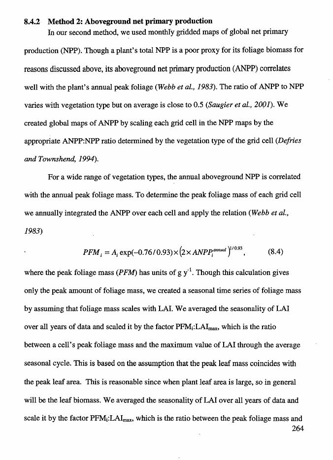
8.4.2 Method 2: Aboveground net primary production In our second method, we used monthly gridded maps of global net primary
production (NPP). Though a plant's total NPP is a poor proxy for its foliage biomass for
reasons discussed above~ its aboveground net primary production (ANPP) correlates
well with the plant's annual peak foliage (Webb et al., 1983). The ratio of ANPP to NPP
varies with vegetation type but on average is close to 0.5 (Saugier et al., 20()1). We
created global maps of ANPP by ~caling each grid cell in the NPP maps by the
appropriate ANPP:NPP ratio determined by the vegetation type of the grid cell (Defries
and Townshend, 1994).
For a wide range of vegetation types, the annual aboveground NPP is correlated
with the annual peak foliage mass. To determine the peak foliage mass of each grid cell
we annually integrated the ANPP over eac;h cell and apply the relation (Webb et al.,
1983)
PFMi =Ai exp(-0.16/0.93)x(2xANP~annual )1'0·93
, (8.4)
where the peak foliage mass (PFM) has units of g i 1• Though this calculation gives
only the peak amount of foliage mass, we created a seasonal time series of foliage mass
by assuming that foliage mass scales with LAI. We averaged the seasonality of LAI
over all years of data and scaled it by the factor PFMi:LAimax, which is the ratio
between a cell's peak foliage mass and the maximum value of LAI through the average
seasonal cycle. This is based on the assumption that the peak leaf mass coincides with
the peak leaf area. This is reasonable since when plant leaf area is large, so in general
will be the leaf biomass. We averaged the seasonality of LAI over all years of data and
scale it by the factor PFMi:LAimax, which is the ratio between the peak foliage mass and 264

the maximum value of LAI through the average seasonal cycle. This is based on the
assumption that the peak leaf mass coincides with the peak leaf area.
The global foliage biomass calculated using this method is sensitive to the input
N~P. Though NPP can be measured directly in field studies on small scales, global NPP
is routinely estimated in carbon cycle and terrestrial ecosystem models. Annual global
NPP from such models typically ranges from 40 to 70 Pg C y-1 (Cramer et al., 1999).
For the current work we used a model that produced an annual NPP of 60 Pg C t 1
(Foley et al., 1996). This is at the upper end of the global NPP range and is chosen to
produce the highest reasonable emissions of methane using this method. According to
Eq. 8.3 we estimate that global foliage mass is 26 Pg C y-1•
8.5 Methane emissions from foliage biomass We transformed the leaf biomass into methane emissions using the emission
rates measured by Keppler et al. (2006). There are two important results of their work
that we considered in our simulation. First, the authors found that emissions nearly
tripled when plant leaves were exposed to direct sunlight, and second there appeared to
be a threshold temperature below which the plants did not produce emissions. To take
into account the first observation we separated each 24-hr day into nighttime and
daylight hours and additionally separated daylight hours into overcast (i.e. indirect
sunlight) and cloud-free (direct sunlight) hours. We also differentiated the fraction of
the leaf canopy that is in direct sunlight from the fraction that is shaded during daylight
hours using a time-dependent vegetation canopy model and applied the appropriate
methane emission rate to each fraction.
265

Figure 8.2. Methane emissions from oxic vegetation source using method (1). Units are Gg CH. month-1.
(a) January; (b) April; (c) July; (d) October.
Though the minimum temperature required for emissions to occur is perhaps unknown,
it seems reasonable to assess the sensitivity of the global emissions to temperature as
the responsible emission mechanism, be it biological, chemical, or physical, is likely
temperature-dependent.
8.6 Results Applying the considerations above, we calculated daily plant emissions over a
0.5x0.5° grid for all terrestrial land surfaces. The respective integrated annual emissions
are 36 and 20 Tg i 1 from Methods 1and2 when we used the mean sunlit and shaded
266

emission rates of 374 and 119 ng CH.i per g (dry weight) h -I reported in Keppler et al.,
(2006). Our annual emissions are considerably lower than those found by the original
study (149 Tg y-1). If we include the reported uncertainties in.the emission rates, the
respectiye emission ranges are 14-60 Tg y-1 and 8-34 Tg i 1• These ranges are similar to
the range of 10-60 Tg i 1 reported by a recent study (Kirschbaum et al., 2006).
The spatial and temporal patterns of emissions are shown for Method 1 in Figs.
8.2 and 8.3. The pattern of emissions estimat~ using Method 2 is similar differing only
quantitatively.
267

We see immediately from Fig. 8.2 that the bulk of the emissions occurs in the
tropics, with concentrations in the Amazonian Basin, equatorial Africa, and the
Indonesian archipelago. We estimate that nearly 90% of all emissions occur between
latitudes of ±30°. Global emissions peak during the northern hemisphere summer
months due to the greater landmass. During the months of June, July, and August, the
"'b E ..,. I u 0)
I-en· c .Q (/) (/)
E w
0.4
0.3
0.2
0.1
-.-Jan -Feb · ·· Mar -tt-Apr -llE- May _._Jun
-+-Jul
-Aug -Sep
.. Oct u--- Nov
Dec
-80 -60 -40 -20 0
Latitude
20 40 60 80 -Annual
Figure 8.3. Latitudinal distribution of monthly methane emissions from vegetation based on leaf biomass
distributions from Method 1.
northern hemisphere's continental Ia:ndmasses (>30°N) contribute nearly 40% of the
global emissions, but they contribute less than 15% of the world's annual emissions. I
During the winter months in each hemisphere, emissions are restricted to latitudes lower
than 30°, while in the summer, emissions in the northern hemisphere extend northwards
268

of 60°. The latitudinal cut-off in emissions is largely a consequence of our choice to
define a minimum temperature, below which we assume plant emissions do not occur.
The smaller leaf biomass during the winter months also limits the latitudinal extent of
the emissions, but this plays only a secondary role since the evergreen coniferous forest
prevalent at high latitudes still contributes leaf matter during the winter months. Thus
the choice of the minimum temperature is important and significantly impacts the global
emissions. If we lower the threshold temperature to 15, 10, and 5°C, the global
emissions are 52, 60, and 66 Tg y-1, respectively. If we further reduce the temperature
to 0°C --- perhaps a less controversial minimum temperature, global emissions increase
only slightly more to 69 Tg y-1• Using our extrapolation scheme, this then appears to be
the maximum emissions we can expect from this source. When we used 0°C as the
minimum temperature in Method 2, emissions increased from 20 Tg i 1 to 36 Tg i 1•
Whether such a minimum temperature exists and what its value may be is one of the
largest sources of uncertainty in our extrapolation process. The sensitivity of the
emissions to this temperature indicates that this needs to be a ~ajor focus of
forthcoming work in this field. In the remainder of the chapter we took the minimum
temperature to be 20°C.
If we categorize the emissions based on land cover type (Fig. 8.4 ), 41 % of the
total are from grasslands and wooded grasslands, while another 32% are from broadleaf
evergreen forests. The only other land type of major significance is croplands, which
contributes 10% of the global emissions. There are small differences between these
values and those calculated using Method 2; 31 %, 42%, and 12%, respectively. These
269

..... ':>.
10
'I 8 u O> I-(/)
c 0
"Ui .~ E w
6
4
2
0 BEF CEF HOF TUN CFW V\/GR GRA BAG SHG CRP BDF
J!igure 8.4. Distribution of oxic methane emissions according to vegetation type. BEF=broadleaf
evergreen forest; CEF=coniferous evergreen forest; HDF=high-latitude deciduous forest;
CFW=coniferous evergreen forest and woodland; WGR=wooded grassland; GRA=grassland; BAG=bare
ground; SHG=shrubs and bare ground; CRP=cultivated crops; BDF=broadleaf deciduous forest and
woodland.
distributions are comparable to Keppler et al. (2006), who estimated tropical forests
(roughly equal to our broadleaf evergreen forests) and grasslands respectively
contribute about 50% and 26% to the total.
8. 7 Emissions from non-wetlands The possibility exists that if this plant source is real, it may already be partly
counted as a component of the flux measured from wetlands and rice paddies.
270

According to this thought, only a fraction of the aerobic plant emissions would be
considered new, with the remaining fraction folded into the previously known wetland
emissions. We estimated what the upper limit to this latter fraction. is by tallying the
plant emissions that occur on land areas designated as either wetlands or rice paddies.
For this purpose we used the global distribution of wetlands by Matthews and Fung,
( 1987) and a distribution of rice paddy areas by Matthews et al. ( 1991 ), both mapped on
a one-degree grid. Using the emissions from Method 1 we found that 8.8 Tg out of the
annual 36 Tg are from these land areas, which leaves a minimum of 27 Tg or 76% of
the total oxic source that would be construed as a new source to be added to the global
budget. This percentage increased to 78% when we used the set of oxic emissions
estimated using a minimum temperature of 0°C as only 15 Tg out of 69 Tg lie within
these regions. Thus even if the measured methane release from rice fields and wetlands
already includes flux from the oxic source, the majority of this source is still
unaccounted for in the present methane budget as it is released from non-flooded
regions.
8.8 Top-down constraints on plant emissions We also investigated whether our estimates of plant emissions were consistent
with the known global methane and isotopic budget. Global fluxes from individual
methane sources are widely uncertain due to the spatial and temporal variations of the
sources. Collective emissions from all sources vary according to budget but typically lie
between 500 -and 600 Tg i 1 (Denman et al., 2007). Better constraints on the global rate
are found through inverse techniques that deconvolve the source from the record of
271

atmospheric methane. From these techniques the global emission rate is found to be
around 550 Tg i 1 (Dlugokencky et al., 1998; Khalil and Butenhoff, 2007).
":",..,
700..--~~~~~~~~~~~~~~~~~~~~~~---,
600+-~~~~~~~~~~~~~~~~~~~~~~----j
.. 500 0 •Inverted ~ 400
i 300 .e ·i 200
~ GBA+149 T g/y
o GEIA+Metho d 1
r:;i GEIA+Metho d 2
IJ.I
100
0 Global NP NM Nf sr SM SP
Figure 8.S. Distribution of amended-methane budget against sources derived from an inversion of the
atmospheric methane record. To the base methane budget (global source= 487 Tg CI!i i 1) estimates of
the oxic source were added. Solid black= inverted sources; diagonal pattern= base budget plus mean
Keppler et al. (2006) vegetation estimates; no pattem=base budget plus method 1 estimates; dappled
pattem=base budget plus method 2 estimates.
The geographical distribution of the source can be found by inverting the·
twenty-year record of methane (see Chapter 2). Results from such an inversion using a
low-resolution model are shown in Fig. 8.5 for the major atmospheric compartments.
Alongside the inverted emissions we place bottom-up estimates of the methane
distribution using the emissions calc'1;llated in this work and those from Keppler et al
(2006). As the oxic source is just one of many sources, we added the oxic emissions to a
gridded global methane budget (Fung et al., 1991) which included contributions from
nearly all other methane sources and totals 487 Tg y-1• Total emissions using the
272

respective estimates from Methods 1, 2, and Keppler et al (2006), are 507, 523, and 639
Tg t 1, while the total inverted source is 554 Tg y-1
• Although the geographical
distribution of each data set is simil~, the sources computed from Methods 1and2 are
arguably in better agreement with the inverted sources, though all three data sets
overestimate the tropical source and underestimate the middle latitude source.
8.8.1 Historical constraints from ice-core record A more rigid constraint on plant emissions comes from the methane budget
during the pre-industrial era when emissions from anthropogenic sources were minimal.
Measurements of o13C}4 in the Law Dome ice-core of Antarctica have recently been
used to constrain the pyrogenic and biogenic sources of methane during the late
preindustrial Holocene (0 to 1700 A.D) (Ferretti et al., 2005). Based on these isotope
measurements and the cotemporaneous atmospheric methane record, pyrogenic and
biogenic emissions were estimated to be 25 and 195 Tg t 1, respectively, during the
period 0 to 1000 A.D. The strength of the pyrogenic emissions was somewhat
surprising as it is nearly twice the size of previous estimates ( Chappellaz et al., 1993;
Houweling et al., 2000) but falls to 10 Tg f 1 by the year 1700 A.D.
273

20
10
Upper I imit of oxic emissions
i Average bottom-up estimate of S0 from current vvork
... Zero pyrogenic emissions ~ 0 a> t-~ -10 en
-20 . . . . . . . . . . . . . ................................................................ . I
: M ean S0 estimate of Keppler et al. 2006
-30 0 25 50 100 125 150
Figure 8.6. Sensitivity of the historic pyrogenic source (Sp) to the strength of the oxic source flux (S.).
Pyrogenic sources are calculated for the time period 1700-1800 A.D. from the ice-core isotope record and
assuming difference source strengths for the oxic source. If oxic emissions exceed 64 Tg CH. y-1,
pyrogenic emissions are forced below zero. Likely, pyrogenic emissions are near 10 Tg CH. y-1 during
this time, which constrains the oxic source to be no greater than 25 Tg CH. y-1. This agrees with our
bottom-up estimates from Methods 1 and 2.
How do these emissions change if we now consider the terrestrial vegetation
source and include it in the source reconstruction during this time? Following Ferretti et
al. (2005) we use a one-box non-equilibrium atmosphere model (La,ssey et al., 2000) to
estimate o13C of the global methane source from the ice-core measurements. The model
includes isotopic fractionation due to differences between the reaction rates of OH with
12CI4 and 13Cf4. To ensure that differences between the pyrogenic and biogenic
274

emissions computed here and those reported above are due only to the inclusion of the
oxic methane source, we adopted model parameter values from Ferretti et al. (2005 ):
kn/k12=0.9926, 't = 7.6 y, Sp=20 Tg y·1 , o13Cbiogenic= -60%0, 013Cpyrogenic= -20%0, and
o13Crossn= -40%0, where kn is the rate coefficient between OH and isotope nCRi , 't is the
methane atmospheric lifetime, Sp is the late pre-industrial Holocene rate of methane
emissions from fossil fuels, and o13Cx is the o13C value for source x. We added to this
mix o13Cvegetation=-50%o, which is the reported weighted o13C value for oxic vegetation
emissions assuming a C3:C4 plant ratio of 60:40 (Keppler et al., 2006). We
parameterized the isotope and atmospheric methane ice-core records with fits that
produce correlation coefficients better than 0.99 and use these as inputs to the model.
Over the period 0 to 1000 A.D., the fit to the isotope record is near constant at o13C=-
47.3%o.
When we set the plant emissions to zero and ran the model, the respective
pyrogenic and biogenic emissions were 24 and 192 Tg i 1 (during0 to 1000 A.D.),
nearly identical to the above emissions as required. As we increased the plant emissions
from zero, the pyrogenic and biogenic emissions decreased as necessary to balance the
source and isotope budget. In fact, as we continued to increase plant emissions, the
isotope budget was only satisfied if the pyrogenic emissions fell to below zero. This is
so since plant emissions are enriched relative to the o13C value of the global source,
which requires a reduc~ contribution from the even more enriched pyrogenic source.
We found that if the pyrogenic emissions are to remain positive throughout the length of
the isotope ice core record, the plant emissions cannot exceed 64 Tg y·1 to
275

accommodate the dip in o13C that occurs around 1800 (Fig. 8.6). Furthermore, it is more
reasonable to constrain plant emissions to rates that produce pyrogenic emissions of at
least 10 Tg y-1 and not zero, since pre-industrial biomass burning and wildfires are
thought to contribute at least this amount (Chapellaz et al., 1993; Houweling et aL,
2000). With this new constraint, we calculated that annual plant emissions can not
exceed 25 Tg y-1 and certainly must be much lower than the original estimate of 149 Tg
y-1• When we assigned this latter value to the plant source we found that the predicted
pyrogenic flux is -21 Tg i 1, which turned the pyrogenic source to a sink, which is
clearly unphysical. Our limit is somewhat lower than a recent estimate by Ferretti et.al.
(2006) who estimated an upper limit of 46 Tg t 1
The results of our ice core analysis also corroborates the bottom-up estimates
(36 and 20 Tg t 1, Method 1 and 2) from above, as the mean of these two estimates (28
Tg f 1) is very close to the threshold estimate of 25 Tg i 1
. In addition, a methane
budget that includes plant emissions of this order is in better agreement with the
expected pyrogenic source than a budget without. When we ran the atmospheric model
with our mean estimate of 28 Tg i 1 over the steady-state years of 0 to 1000 A.D., the
predicted pyrogenic flux during this time is 16 Tg y-1• This agrees ~etter with the
expected value of 15 Tg i 1 (Houweling et al., 2000) relative to the predicted flux from
a model run with no plant source (24 Tg i 1). The magnitude of the plant source is not
only consistent then with the known methane budget, but it brings the budget into better
agreement with expectations. The predicted biogenic emissions, which include
contributions from wetlands, termites, ruminants, and rice agriculture, are 170 Tg i 1,
276

which is consistent with estimates of this source, (Chappellaz et al., 1993; Houweling et
al., 2000). Thus-these results combined with those from our extrapolations support the
view that emissions from terrestrial plants are modest and can be readily accommodated
within the methane budget.
277

Chapter 9 - Conclusion
9.1 Summary The work presented in these chapters represents an attempt to better understand the
changing source and sink strengths of atmospheric methane. To do so we used ·
measurements of trace gases at remote background stations from four different
sampling networks. These networks include the Oregon Graduate Institute (OGI), the
National Oceanic and Atmospheric Administration's Global Monitoring Division
(NOAA-GMD), the Atmospheric Lifetime Experiment/Global Atmospheric Gas
Experiment/ Advanced Global Atmospheric Gas Experiment (ALE/GAGE/ AGAGE),
and the Gas .... of the Commonwealth Scientific Institute of Research Organization
(CSIR.0-GASLAB). In most cases the measurement time series extended back to the
early 1980' s. In many cases we joined measurements from different networks. In this
way not only were we able to create longer time series than exists for a single network,
we were also able to test how differences between networks influenced the results of
our modeling simulations. In this manner we could assess the robustness of the modeled
features.
As a starting point for our investigation we inverted the recent atmospheric
history of C~. For this we created a time series of measurements that stretched back to
1981 and continued to recent years. The composite record was produced by joining the
278

OGI and NOAA data sets at the monitoring sites common to both networks. The trend
of C~ drops rapidly over this period. To explain this behavior we used a chemical-
transport model and ran it in inverse mode. In this configuration, the model uses as
inputs the time series of C~ measurements in each of the six major latitudinal air
masses (i.e. north and south polar latitudes (65-90 N,S), north and south mid-latitudes
(30-65 N,S), and north and south tropics(0-30 N,S). We found that with OH levels
constant, the declining trend of C~ is consistent with stable emissions over the 23-year
period of ~tudy. Emissions were constant at - 550 Tg y-1• This behavior of C~ can be
explained by the approach of atmospheric C~ to ·steady state. That is the sink of CH4, . !
primarily the CH4+0H reaction, is c:oming into balance with emissions. We. showed
using the global average methane record and a simple one-box model, that the recent
history of atmospheric C~ is consistent with a constant global CH4 source strength of
550 Tg i 1 and a total lifetime of 8.9 yr.
However, an alternate scenario is that both CH4 sources and lifetime are
changing simultaneously. Under this scenario, if the lifetime of C~ were increasing
over this time period, the global source strength of CH4 would be decreasing to
' maintain the trends observed in the atmospheric record. Thus an independent analysis of
the trends of C~' s sources and sinks is required to assess whether atmospheric CH4 is
indeed in steady stat~. This was the task of the remainder of the dissertation.
We first examined the possibility that the main sink of atmospheric CH4, its
reaction with the hydroxyl radical OH, is changing. Since the atmospheric lifetime of
OH is so short, direct measurements of OH provide only local information about its
279

atmospheric abundance. Furthermore, no long-term systematic record of atmospheric
OH is available globally. And while it is possible to model the long-term trends of
atmospheric OH based on its chemical production and removal pathways, this requires
additional information about the trends and abundances of any number of chemical
species over large spatial and temporal scales. Thus any such effort suffers from large
uncertainties.
In this work we inferred the history of OH using a proxy gas, the chlorinated
solvent, methylchloroform (CH3CCh). The useful properties of this gas include, it is
nearly entirely anthropogenically produced through industrial processes, which has the
advantage that good records exist on its production history. Secondly, it is removed
almost entirely by OH. And finally, it has a relatively short lifetime (-5 yr) so its
atmospheric abundance should reflect changes in OH levels. We again used our
chemical-transport model. We used as inputs, the emissions record of CH3CCh based
on a release history of the solvent, and the long-term ALE/GAGE/ AGAGE CH3CCh
measurements. Over the time period 1978 - 2008, we found that OH was not constant
but had strong interannual variability. We estimated the average trend of OH over this
period to be -0.43 pm 0.21 % i 1• The history of OH we derived however is more
complex than this single trend suggests. OH levels were mainly flat or even slightly
rising from the beginning of the model period to 1990. From 1990 to 1999, OH levels
drop by about 10%. This drop is simulated using not just the ALE/AGAGE/AGAGE
measurements, but also the OGI and NOAA-GMD records, though trends estimated
280
from the latter records were not significant due to the shorter time series of MCF
measurements available.
We tested to see how sensitive the OH trend is to factors such as
modeling/inversion scheme, temperature, calibration, and emissions history. Within
known trends and uncertainties in these drivers, the negative OH trend remains. We
found that the OH trend disappears if the MCF calibration scales was in error by 10% or
more. Quoted uncertainty in the AGAGE calibration is 3%, and within this range, the
trend is still statistically significant. Besides the calibration, the largest uncertainty that
would affect our calculation is the timing of MCF release from production. To the
extent that the uncertainty of this timing was factored into the error estimates of the
McCulloch and Midgley (2001 i emission record, the OH trend remains within this
uncertainty. We also conducted additional experiments on the sensitivity of emission
release by constructing alternative release histories using an exponential release
function. In these scenerios the delay between production and release is determined by a
decay constant. We increasing the decay constant for example, we can increase the lag
between production and release. Our experiments showed that no single decay constant
was able to simulate emissions that were consistent with inverted emissions from a
zero-OH trend modeling run. However this does not rule out the possibility that the
decay constant changes over the years. Future work needs to investigate this possibility.
If the lifetime of atmospheric CH4 is changing due to a trend in atmospheric
OH, then individual C~ sources must change to compensate. In particular, ~ome
281

sources must be decreasing in time. The next chapters of the dissertation investigated
individual sources.
We used a novel technique to study emissions from biomass burning. Biomass
burning is a major source of atmospheric carbon monoxide and hydrogen. In fact this
pair of gases share common sources, and yet are principally removed by different
mechanisms, oxidation by OH for CO, and soil deposition for H2. We found that when
we inverted the long-term time series of atmospheric measurements for both gases, the
simulated emission history of each coincided to a high degree, both peaking and falling
at the same time. We limited our analysis to the tropics where biomass burning is
strongest and the dominant source of both gases. Here we found that our simulated CO
and H2 emissions had seasonal cycles that peaked in the dry seasons of both
hemispheres, consistent when emissions from biomass burning occur. Also, a
comparison between our inverted emissions and satellite-derived fire counts, showed
that the Syasonal cycles and cycle strength were consistent with fire activity. We
integrated emissions from both the CO and H2 record over the seasonal peaks of each
year. This we took as the estimate of annual biomass burning emissions. The time series
of annual emissions shows that in the southern tropics biomass burning emissions have
increased by roughly 10% over the years 1981 to 1999. This is increase is evident in
both the CO and H2 emission histories. There is no emission trend seen in the northern
tropics. The biggest feature here is a large positive anomaly in 1997 /98. This coincides
with an especially strong El Nino event that produced droughts and wildfires in western
Pacific countries such as Indonesia and Malaysia.
282

One of the largest uncertainties in our biomass burning emission estimates is,
that they rely upon consideration of other CO and H2 emissions in the tropics. These we
must account for. The source with the largest uncertainty is the production of CO and
H2 from the oxidation of isoprene and terpenes. Both of these gases are emitted by
vegetation. The literature includes estimates of global source strengths that vary by a
factor of two. In the tropics, isoprene and terpenes are emitted throughout the year but
emissions peak during the wet season of each hemisphere, which is anti-correlated with
the cycle of biomass burrii.ng. Because the impact of uncertainty on our conclusions is
mitigated. However, we recognize that reducing the uncertainty in isoprene and terpene
emissions is an area that needs considerable effort in the future.
We next investigated the global source strength of methane emission from rice
agriculture. Recent estimates of this source vary widely, by nearly a factor of five in the
latest IPCC report. We used experimental results from our greenhouse and field studies
on factors controlling paddy flux, to create global gridded inventories of CH4 emissions.
Using a wide variety of geospatial agricultural, environmental, and vegetation data, we
constructed gridded input maps and from these estimated methane flux for all areas of
global rice production. Based on ·harvested area and crop phenology we estimated
annual emissions from these fluxes. Our global estimate of 50 Tg i 1 is consistent with
past work and continues the. trend of decreasing estimates of methane from rice
agriculture. One notable result is that emissions in India are more than twice as high as
those in China. This is due to a number of reasons including higher seasonal
temperature averages in India, a larger fraction of rice production managed under
283

continuously flooded conditions, and smaller rate of synthetic fertilizer usage, which we
found in our field studies to retard methane flux.
We next used China as a test case to study how emissions from rice agriculture
have changed over the past few decades. In China, a number of important changes have
occurred that influenced paddy emissions. Starting in the 1970s, synthetic fertilizers
became favored over organic fertilizes which would reduce CH4 emissions (though
increase N20 emissions). To improve crop yields and conserve water, the practice· of
mid-season drainage was started in the early 1980s and spread widely throughout China
to the present. We considered these changes and others on paddy emissions. We found
that methane emissions decreased by about 15 Tg y-1 from1980. to the present. This
would contribute to the general reduction in methane emissions required if OH levels
decreased as predicted here.
Finally we considered the potential of vegetation as a source of methane. Direct
measurements of CH4 flux from plants are limited. Here we used the reported fluxes
from Keppler et al. (2006) to assess whether global vegetation could be an important
component of the global C~ budget. We found through bottom-up methods that global
emissions ranged from 20 to 36 Tg y-1• We tested these estimates using the pre
industrial atmospheric record of CH4 and o13CH4 measured from ice cores. The ice core
records constrain the natural source strength of CH4• We estimate an upper limit on
vegetation emissions of 25 Tg y-1 assuming that natural biomass burning emissions
were 10 Tg i 1• This upper limit is consistent with our bottom-up estimates. We
conclude that terrestrial plants may be a significant source of methane, though not as
284

large as previous studies indicate. We note that recent studies found a strong correlation
between UV radiation and methane flux. This will be an important connection to model
in future work.
9.2 Closing thoughts The picture that emerges from this work dispels the notion that the sources and
sinks of atmospheric methane have been constant over the past couple decades despite
the fact that the recent behavior of atmospheric Cl4 is consistent with steady state
conditions. There appears to be changes on the order of 10% that have occurred in the
major sink of CH4 and some of its important anthropogenic sources. In the south
tropics, where we estimate emissions from biomass burning are increasing, there must
be some offsetting decreasing emissions there as well , as our inverse modeling of Cl4
shows that emissions must be constant in the southern hemisphere. If vegetation does
. emit Cl4 at rates suggested by this work, then the reduction in CJ4 emissions due to
the deforestation of tropical forests could produce the required balance.
In closing, we offer the following perspective. Oftentimes, we miss the proverbial
forest for the trees. We miss the bigger picture while seeing only the smaller
components that compose it. Here the reverse may be true. The bigger story is that
atmospheric methane is stabilizing. We may erroneously take this to mean that the
component sources and sinks are doing the same. In so doing, not only might we miss a
rich underlying story of sources and sinks that are bubbling underneath a smooth
surface, but in the future these sources (or sinks) may break through and again push
atmospheric levels of methane upwards. Here~ the details are important, it is important
285

to see the trees for the forest. This investigation of the sources and sinks of atmospheric
methane hopefully will remind us of the complexity of Earth's atmosphere and the
relations that bind it to our own activities.
286

References
AFEAS, 2001. Production, Sales, and Atmospheric Release of Flurocarbon through 2000. AFEAS, Arlington, VA (see www.afeas.org).
Akiyama, H., K. Yagi, and X.Y. Yan, 2005. Direct N20 emissions from rice paddy fields: Summary of available data, Global Biogeochem. Cycles, 19, GB1005, doi: 10.1029/2004GB002378.
Alexander, R., and A.C. Millington, 2000. Vegetation Mapping. Chichester, England: John Wiley.
Allan, W., et al., 2005. Interannual variations of 13C in tropospheric methane: Implications for a possible atomic chlorine sink in the marine boundary layer. J. Geophys. Res., 110, doi:10.1029/2004JD005650.
Andreae, M.0., 1991. Biomass burning: Its history, use, and distribution and its impact on environmental quality and global climate, in Global Biomass Burning: Atmospheric, Climatic, and Biospheric Implications, J.S. Levine, ed., Mlt Press, Cambridge, Mass. 1991.
Andreae, M.O., and P. Merlet, 2001. Emission of trace gases and aerosols from biomass burning, Global Biogeochem. Cycles, 15, 955-966.
Angell, J. K. ,2000. Difference in radiosonde temperature trend for the period 1979-1998 of MSU data and the period 1959-1998 twice as long, Geophys. Res. Lett., 27, 2177-2180.
Arellano Jr., A.F., P.S. Kasibhatla, L. Giglio, G.R. van der Werf, J.T. Randerson, and G.J. Collatz, 2006. Time-dependent inversion estimates of global biomass-burning CO emissions using Measurement of Pollution in the Troposphere (MOPITT) measurements, J. Geophys. Res., 111, D09303, doi:10.1029/2005JD006613.
Arino, 0., and J.-M·. Rosaz, 1999. 1997 and 1998 World ATSR Fire Atlas using ERS-2 ATSR-2 data, in Proceedings of the Joint Fire Science Conference, Boise, Idaho, p. 177-182, University of Idaho and the International Association of Wildland Fire.
Aslemann I, and P .J. Crutzen, 1989. Distribution of natural freshwater wetlands, J. Atm. Chem., 8, 307-358.
Aucott, M.L, A. McCulloch, T.E. Graedel, G. Kleiman, P.M. Midgley, Y.-F. Li, 1992. Anthropogenic emissions of trichloromethane (chloroform, CH Ch) and
287

chlorodifluoromethane (HCFC-22): Reactive Chlorine Emissions Inventory, J. Geophys.Res. 104,8405-8416, 1999
Bauer, K., W. Seiler, and H. Giehl, 1979. CO Produktion hoherer Pflanzen an naturlichen Standorten, Z. Pflanzenphysiol., 94, 219-230.
Bergamaschi, P ., R. Hein, M. Heimann, and P .J. Crutzen, 2000a. Inverse modeling of the global CO cycle. 1. Inversion of CO mixing ratios, J. Geophys. Res., 105, 1909-1927.
Bergamaschi, P., R. Hein, C.A.M. Brenninkmeijer, and P.J. Crutzen, 2000b. Inverse modeling of the global CO cycle 2. Inversion of 13C/12C and 180/160 isotope ratios, J. Geophys. Res., 105, 1929-1945.
Bousquet, P., D.A. Hauglustaine, P. Peylin, C. Carouge, and P. Ciais, 2005. Two decades of OH variability as inferred by an inversion of atmospheric transport and chemistry of methyl chlorofo!Jll, Atmos. Chem. Phys., 5, 2635-2656.
Bouman, A. F., 1990. Soils and the Greenhouse Effect, 515 pp., Wiley, Chichester, UK. .
Brohl, C., S. R. Drayson, J.M. Russell Ill, P. J. Crutzen, J.M. Mcinerney, P. N. Purcell, H. Clande,, H. Gemandt, T. J. McGee, I. S. McDermid, and M. R. Gunson, 1996. Halogen Occulatation Experiment ozone channel validation, J. Geophys. Res., 10217-10240.
Butenhoff, C.L., 2002. Development and application of a two-dimensional atmosphereocean transport box model to CChF and CChF2, Master's Thesis, Portland State University, Portland, OR.
Butler, J.H., M. Battle, M. L. Bender, S. A. Montzka, A.D. Clarke, E. S. Saltzman, C. M. Sucher, J.P. Severinghaus, and J. W. Elkin, 1999. A record of atmospheric halocarbons during the twentieth century from polar fim air, Nature, 399, 749.
Cai, Z.C, G.X. Xing, X. Y. Yan, H. Xu, H. Tsuruta, K. Yagi, and K. Minami, 1997. Methane and nitrous oxide emissions from paddy fields as affected by nitrogen fertilizers and water management, Plant Soil, 196, 7-14.
Cao, M., J.B. Dent, and O.W. Heal, 1995. Modelling methane emissions from rice paddies, Global. Biogeochem. Cycles, 9, 183-195.
Carmo, J.G., M. Keller, J.D. Dias, P.B. Carmargo and P. Crill. 2006. A source of methane from upland forests in the Brazilian Amazon, Geophys. Res. Lett., 33, L04809.
288

Cramer, W., D.W. Kicklighter, A. Bondeau, B. Moore III, G. Churkina, B. Nemry, A. Ruimy, and A.L. Schloss, 1999. Comparing global models of terrestrial net primary production (NPP): overview and key results, Global Change Biol., 5, 1-15.
Cheng W., H. Sakai, A. Hartley, K. Yagi, and T. Hasegawa, 2008. Increased night temperature reduces the stimulatory effect of evelevated carbon dioxide concentration on methane emission from paddy soil, Glob. Change. Bio., 14, 644-656.
~hristy, J.R., R.W. Spencer, and W.D. Braswell, 2000: MSU tropospheric temperatures: Dataset construction and radiosonde comparisons. J. Atmos. Ocean. Technol., 17, 1153-1170.
Cicerone, R.J ., and J .D. Shetter, 1981. Sources of atmospheric methane: Measurements in rice paddies and a discussion, J. Geophys. Res., 86, 7203-7209.
Conrad, R., W. Seiler, G, Bunse, and H. Giehl, 1982. Carbon monoxide in sea water (Atlantic Ocean), J. Geophys. Res., 87, 8839-8852.
Cooper, L.N., L.P. Steele, R.L. Langenfelds, D.A. Spencer and M.P. Lucarelli, 1999. Atmospheric methane, carbon dioxide, hydrogen, carbon monoxide and nitrous oxide from Cape Grim flask air samples analysed by gas chromatography. Baseline Atmospheric Program (Australia) 1996, edited by J.L. Gras, N. Derek, N.W. Tindale and A.L. Dick, pp 98 - 102, Bureau of Meteorology and CSIRO Atmospheric Research, Melbourne, Australia, 1999
Crutzen, P.J., and M.O. Andreae, 1990. Biomass burning in the tropics: Impact on atmospheric chemistry and biogeochemical cycles, Science, 250, 1669-1678.
Crutzen, P.J., and J. Lelieveld, 2001. Human impacts on atmospheric chemistry, Annu. Rev. Earth Planet Sci., 29, 17-45.
Crutzen, P.J., A.C. Delany, J. Greenberg, P. Haagenson, L. Heidt, R. Leub, W. Pollock, W. Seiler, A. Wartburg, and P. Zimmerman, 1985. Tropospheric chemical composition measurements in Brazil during the· dry season, J. Atmos. Chem., 2, 233-256, 1985.
Crutzen, P.J., E. Sanhueza and C.A.M. Brennillkmeijer. 2006. Methane production from mixed tropical savanna and forest vegetation in Venezuela. Atmos. Chem. Phys. Discuss., 6, 3093-3097.
Defries, R. S. and J.R.G. Townshend, 1994. NOVI-derived land cover classification at a global scale, Int. J. Remote. Sens., 15, 3567-3586.
Denman, K.L., G. Brasseur, A. Chidthaisong, P. Ciais, P.M. Cox, R.E. Dickinson, D. Hauglustaine, C. Heinze, E. Holland, D. Jacob, U. Lohmann, S Ramachandran, P.L. da
289

Silva Dias, S.C. Wofsy and X. Zhang, 2007: Couplings Between Changes in the Climate System and Biogeochemistry. In: Climate Change 2007: The Physical Science Basis. Contribution of Working Group I to the Fourth Assessment Report of the Intergovernmental Panel on Climate Change [Solomon, S., D. Qin, M. Manning, Z. Chen, M. Marquis, K.B. Averyt, M.Tignor and H.L. Miller (eds.)]. Cambridge University Press, Cambridge, United Kingdom and New York, NY, USA.
Ding,A., C.R.Willis, R.L. Sass, and F.M. Fisher,1999. Methane emissions from rice fields: Effect of plant height among several rice, Glob. Biogeochem. Cycles, 13, 1045.
Dlugokencky, E.J., E.G. Dutton, P.C. Novelli, P.P. Tans, K.A. Masarie, K.O. Lantz, and S. Madronich, 1996.Changes in CH4 and CO growth rates after the eruption of Mt. Pinatubo and their link with changes in tropical tropospheric UV flux, Geophys. Res. Lett., 23, 2761-2764.
Dlugokencky, E.J., K.A. Masarie, P.M. Lang, and P.P. Tans, 1998. Continuing decline in the growth rate of the atmospheric methane burden, Nature, 393, 447-450.
Dlugokencky, E.J., B.P. Walter, K.A. Masarie, P.M. Lang, and E.S. Kasischke, Measurements of an anomalous global methane increase during 199~, Geophys. Res. Lett., 28, 499-502. .
Dlugokencky, E.J., S. Houweling, L. Bruhwiler, K.A. Masarie, P.M. Lang, J.B. Miller, and P.P. Tans, 2003. Atmospheric methane levels off: Temporary pause or a new steady-state?, Geophys. Res. Lett., 30, doi.1029/2003GL018126.
Dlugokencky, E.J., P.M. Lang, and K.A. Masarie, 2009. Atmospheric Methane Dry Air Mole Fractions from the NOAA ESRL Carbon Cycle Cooperative Global Air Sampling Network, 1983-.2008, Version: 2009-06-18, Path: ftp://ftp.cmdl.noaa.gov/ccg/ch4/flask/event/.
Duncan, B.N., R.V. Martin, A.C. Staudt, R. Yevich, and J. A. Logan, 2003. Interannual and seasonal variability of biomass burning emissions constrained by satellite observations, J. Geophys. Res., 108, 4100, doi: 10.1029/2002JD002378.
Emmons, L.K., M.N. Deeter, and J.C. Gille, 2004. Validation of measurements of pollution in the troposphere (MOPITI) CO retrievals with aircraft in situ profiles, J. Geophys. Res., 109, 003309, doi:10.1029/2003JD004101.
FAO (2005) FAOSTAT Agricultural Data
290

Ferretti, D.F., J.B. Miller, J.W.C. White et al., 2005. Unexpected changes to the global methane budget over the past 2000 years, Science, 309, 1714-1717.
Fleming, E.L, S. Chandra, M.R. Shoeberl, and J.j. Barnett, 1988. Monthly mean global climatology of temperature, wind, geopotential height, and pressure for0-120 km, NASA Technical Memorandum 100697.
Foley, J.A., l.C. Prentice, N. Ramankutty, S. Levis, D. Pollard, S. Stich, and A. Hazeltine, 1996. An integrated biosphere model of the land surface process, terrestrial carbon balance, and vegetation dynamics, Global Biogeochem. Cycles, 10, 603-628.
Forster, P., V~ Ramaswamy, P. Artaxo, T. Berntsen, R. Betts, D.W. Fahey, J. Haywood, J. Lean, D.C. Lowe, G. Myhre, J. Nganga, R. Prinn, G. Raga, M. Schulz and R. Van Dorland, 2007. Changes in Atmospheric Constituents and in Radiative Forcing. In: Climate Change 2007: The Physical Science Basis. Contribution of Working Group I to the Fourth Assessment Report of the Intergovernmental Panel on Climate Chan8e [Solomon, S., D. Qin, M. Manning, Z. Chen, M. Marquis, K.B. Averyt, M.Tignor and H.L. Miller (eds.)]. Cambridge University.
Francey, R.J., L.P. Steele, R.L. 'Langenfelds and B.C. Pak, High precision long-term monitoring of radiatively-active trace gases at surface sites and from ships and aircraft in the Southern Hemisphere atmosphere. J. Atmos. Science., 56, 279-285, 1999.
Frankenberg, C., J.F. Meirink, M. vanWeele, U. Platt and T.Wagner. 2005. Assessing methane emissions from global space-borne observations. Science, 30~:1010-1014
Galanter, M., H. Levy II, and G.R. Carmichael, 2000. Impacts of biomass burning on tropospheric CO, NOx and 03, J. Geophys. Res., 105, 6633-6653.
Gregoire, J.-M., K. Tansey, and J.M.N Silva, 2003. The GBA2000 initiative: Developing a global burned areas database from SPOT-VEGETATION imagery, Int. J. Remote Sens., 24, 1369-1376.
Guenther A, Hewitt CN, Erickson D, Fall R, Geron C, Graedel T, Harley P, Klinger L, Lerdau M, McKay Wa, Pierce T, Scholes B, Steinbrecher R, Tallamraju R, Taylor J, Zimmerman P 1995. A Global-Model of Natural Volatile Organic-Compound Emissions, J. Geophys. Res., 100 (D5): 8873-8892.
Gupta, M., et al., 1997. 12C/13C kinetic isotope effects in the reactions of Clti with OH and Cl. Geophys. Res.Lett., 24, 2761-2764.
Hamburger, J. 2002. Pesticides in China: a growing threat to food safety, public health, and the environment. China Environment Series 5: 29-44.
291

Hansen, J., M. Sato, R. Ruedy, A. Lacis, and V. Oinas, 2000. Global warming in the twenty-first century: An alternative scenario, Proc. Natl. Acad. Sci., 97, 9875-9880.
Hanst, P.L., J.W. Spence, and 0. Edney, 1980. Carbon monoxide production in photooxidation of organic molecules in the ~r. Atmos. Environ. 14, 1077-1088.
Hao, W.M., and M-H Liu, 1994. Spatial and temporal distribution of tropical biomass burning, Global Biogeochem. Cycles, 8, 495-503.
Hauglustaine, D. A. et al., 1998. MOZART, a global chemical transport model for ozone and related chemical tracers 2. Model results and evaluation, J. Geophys. Res., 103, 28,291-28,335.
Hauglustaine D.A. and D.H. Ehhalt, 2002. A three-dimensional model of molecular hydrogen in the troposphere, 107, 4330, doi.10.1029/2001JD001156.
Hoelzemann, J.J., M.G. Schultz, G.P. Brasseur, and C. Granier, 2004. Global Wildland Fire Emission Model (GWEN): Evaluating the use of global area burnt satellite data, J. Geophys. Res., 109, D14S04, doi:1029/2003JD003666.
Holzapfel-Pschom, A., and W. Seiler, 1986. Methane emission during a cultivation period from an Italian rice paddy, J. Geophys. Res., 91(Dll), 11,803-11,814.
Houweling, S., F. Dentener, F., and J. Lelieveld, 2000. Simulation of pre-industrial atmospheric methane to constrain the global source strength of natural wetlands, J. Geophys. Res., 105, 17243-17255.
Huang, Y ., Z. Wen, Z. Xunhua, H. Shenghui, and Y. Y ongqiang, 2006. Estimates of methane emissions from Chinese rice paddies by linking a model to GIS database, Acta Ecol. Sinica, 26, 980-988.
Huang, Y., W. Zhang, Z Zheng, J. Li, and Y. Yu, 2004. Modeling methane emission from rice paddies with various agricultural practices, J. Geophys. Res., 109, D08113, doi: 10.1029/2003JD004401.
Horowitz, L.W., S. Walters, D.L, Mauzerall, et al., 2003. A global simulation of tropospheric ozone and related tracers: Description and evaluation of MOZART, version 2, J. Geophys. Res., 108(D24), 4784, doi:10.1029/2002JD002853.
Intergovernmental Panel on Climate Change (IPCC), 1990. Climate Change-Scientific Assessment, 365 pp., Cambridge Univ. Press, Cambridge, UK.
292

Intergovernmental Panel on Climate Change (IPCC), 1994. Radiative forcing of climate change and an evaluation of the IPCC IS92. emission scenarios, in Climate Change 1994, edited by J.T. Houghton et al., Cambridge Univ. Press, New York.
Intergovernmental Panel on Climate Change (IPCC), 2007. 2006 IPCC Guidelines for National Greenhouse Gas Inventories, Inst. For Global Environ. Strategies, Hayama, . . Japan.
Ito, A., and J.E. Penner, 2004. Global estimates of biomass burning emissions based on satellite imagery for the year 2000, J. Geophys. Res., 109, D14S05, doi: 10.1029/2003JD004423.
Jacob, D.J., and S.C. Wofsy, 1990. Budgets of reacdtive nitrogen, hydrocarbons, and ozone over the Amazon forest during the wet season, J. Geophys. Res., 95, 16,737-16754.
Kalnay et al., 1996. The NCEP/NCAR 40-year reanalysis project, Bull. Amer. Meteor. Soc., 77, 437-470.
Kanakidou, M., and P .J. Crutzen, 1999. The photochemical _source of carbon monoxide: Importance, uncertainties, and feedbacks, Chemosphere: Global Change Science, i, 91-109.
Karl, T, A. Hansel, T. Mark, W. Lindinger, and D. Hoffmann, 2003. Trace gas monitoring at the Mauna Loa Baseline Observatory using proton-transfer reaction mass spectrometry, lnternat. J. of Mass Spectromet., 223-224, 527-538,.
Karlsdottir, S., and I.S.A. Isaksen, 2000. Changing methane lifetime: Possible cause for reduced growth, Geophys. Res. Lett., 27, 93-96.
Keeling, C.D., R.B. Bacastow, A.E. Bainbridge, C.A. Ekdahl, P.R. Guenther, and L.S. Waterman, 1976. Atmospheric carbon dioxide variations at Mauna Loa Observatory, Hawaii, Tellus, vol. 28, 538-551.
Keppler, F., J.T.G. Hamilton, M. Brass, and T. Rockmann, 2006. Methane emissions from terrestrial plants under aerobic conditions, Nature, 439, doi: 10.1038 ..
Khalil, M.A.K., and R.A. Rasmussen, 1984. Carbon monoxide in the earth's atmosphere: Increasing trend, Science, 224, 54-56.
Khalil, M.A.K., and R.A. Rasmussen, 1988. Carbon monoxide in the earth's atmosphere: Indications of a global increase, Nature, 332, 242-245.
293

Khalil, M.A.K., and R.A. Rasmussen, 1990. Atmospheric methane: Recent global trends, Environ. Sci. Technol., 24, 549-553 ..
Khalil, M.A.K., and RA. Rasmussen, 1991. Methane emissions from rice fields in China, Environ. Sci. Tech., 25, 979-981.
Khalil, M.A.K., and R.A. Rasmussen, 1993. Decreasing trend of methane: Unpredictability of future concentrations, Chemosphere, 26, 803-814.
Khalil, M.A.K., and R.A. Rasmussen, 1994. Global decrease in atmospheric carbon monoxide concentration, Nature, 370, 639-641.
Khalil, M.A.K., and M.J.Shearer, 2000. Sources of methane: An overview, in Atmospheric Methane: Its Role in the Global Environment, edited by M.A.K. Khalil, pp 98-111, Springer, Berlin. ,.
Khalil, M.A.K., R.A. Rasmussen, and M.J. Shearer, 1998a. Effects of production and oxidation processes on methane emissions from rice fields, J. Geophys. Res., 103, 25,233-25,239.
Khalil, M.A. K., R. A. Rasmussen, M. J. Shearer, Z. L. Chen, H. Yao, and·Y. Jun, 1998b. Emissions of methane, nitrous oxide, and other trace gases from rice fields in China, J. Geophys. Res., 103(Dl9), 25,241-25,250.
Khalil, M.A.K., R.A. Rasmussen, M.J. Shearer, R.W. Dalluge, L.X. Ren, and C.-L. Duan, 1998c. Measurements of methane emissions from rice fields in China, J. Geophys. Res., 103, 25,181-25210.
Khalil, M.A. K., M. J. Shearer, R. A. Rasmussen, C. L. Duan, and L. X. Ren, 2008a. Production, oxidation, and emissions of methane from rice fields in China, J. Geophys. Res., 113, GOOA04, doi: 10.1029/2007JG000461.
Khalil, M. A. K., M. J. Shearer, R. A. Rasmussen, L. Xu, and J.-L. Liu, 2008b. Methane and nitrous oxide emissions from subtropical rice agriculture in China, J.. Geophys. Res., 113, GOOA05, doi:10.1029/2007JG000462.
Krol., M. P.J. van Leeuwen, and J. Lelieveld, 1998. Global OH trend inferred from methylchloroform measurements, J. Geophys. Res., 103, 10697-10711.
Krol, M., and J. Lelieveld, 2003. Can the variability in tropospheric OH be deduced from measurements of 1,1,1-trichloroethane (methyl chloroform)?, J: Geophys. Res., 108, 4125, doi:10.1029/2002JD002423.
294

Koyama, T., 1963. Gaseous metabolism in lake sediments and paddy soils and the production of hydrogen and methane, J. Geophys. Res., 68, 3971-3973.
Kurylo, M. J, J.M. Rodriguez, M.O. Andreae, E.L. Atlas, D.R. Blake, J.H. Butler, S. Lal, D.J. Lary, P.M. Midgley, S.A. Montzka, P.C. Novelli, C.E. Reeves, P.G. Simmonds, L.P. Steele, W.T. Sturges, R.F. Weiss, and Y. Yokouchi, 1998. Short-Lived Ozone-Related Compounds, World Meteorological Organization, Geneva.
Lamontagne, R.A., J.W. Swinnerton, and V.J. Linnenboom, 1974. Cl-C4 hydrocarbons in the north and south Pacific, Tellus, 26, 71-77.
Lassey, K.R., D.M. Etheridge, D.C. Lowe, A.M. Smith, and D.F. Ferretti, 2007. Centennial evolution of the atmospheric methane budget: what do the carbon isotopes tell us?, Atmos. Chem. Phys., 7, 2119-2139.
Lassey, K.R., D.C. Lowe, and M.R. Manning, 2000. The trend in atmospheric methane C>
13C and implications for isotopic constraints on the global methane budget, Global Biogeochem. Cycles, 14, 41-49. .
Leff, B., N. Ramankutty, and J.A. Foley, 2004. Geographic distribution of major crops ac;ross the world, Global Biogeochem. Cycles, 18, GB1009, doi: 10.1029/2003GB002108.
Levine, J.S., 1999. The 1997 fires in Kalimantan and Sumatra, Indonesia: Gaseous and particulate emissions, Geophys. Res. Lett., 7, 815-818.
Levine, J.S., and W.R. Cofer, 1999. Borealforestfire emissions and the chemistry of the atmosphere. Fire, Climate Change and Carbon Cycling in the North American Boreal, Ecological Studies Series, Springer-Verlag, New York.
Li, C., A. Mosier, R. Wassman, Z. Cai, X. Zheng, Y. Huang, H. Tsuruta, J. Boonjawat, and R. Lantin, Global Biogeochem. Cycles, 18, GB 1043, doi: 1029/2003GB002045.
Li. C., J. Qiu, S. Frolking, X. Xiao, W. Salas, B. Moore III., S. Boles, Y. Huang, and R. Sass, 2002. Reduced methane emissions from large-scale changes in water management of China's rice paddies during 1980-2000, Geophys. Res. Lett., 29, 1972, doi: 10.1029/2002GLO 15370.
Liang, S. 2004. Quantitative remote sensing of land surfaces. Hoboken, NJ: WileyInterscience.
Liss, P.S., and ~.G. Slater, 1974. Flux of gases across the air-sea interface, Nature, 247, 181-184.
295

Lobert, J.M., W. C. Keene, J. A. Logan, and R. Yevich, 1999. Global chlorine emissions from biomass burning: Reactive Chlorine Emissions Inventory, J. Geophys. Res., 104(D7), 8373-8389, doi:10.1029/1998JD100077.
Logan, J.A., 1983. Nitrogen oxides in the troposphere: Global and regional budgets, J. Geophys. Res., 88, 10785-10807.
Lowe, D. C., 2006. Global change: A green source of surprise, Nature, 439, 148-149.
Madronich, S. 1993. The atmospl1ere and UV-B radiation at ground level, Environmental UV Photobiology, Plenum Press, 1-39.
Mather, P.M., 1995. Terra 2 Understanding the Terrestrial Environment. Chichester, England: John Wiley.
Matthews, E., and I. Fung, 1987. Methane emissions from natural wetlands: global distribution, area, and environmental characteristics of sources, Global Biogeochem. Cycles, 1, 61-86.
Matthews, E., I. Fung, and J. Lerner, 1991. Methane emission from-rice cultivation: Geographic and seasonal distribution of cultivated areas and emissions, Global Biogeochem. Cycles, 5, 3-24.
Matthews, R.B., R. Wassmann, and J. Arah, 2000. Using a crop/soil simulation model and GIS techniques to assess methane emissions from rice fields in Asia. I. Model development, Nut. Cycling Agroecosys., ~8, 141-159.
McCulloch, A., P.M. Midgley, and D.A. Fisher, 1994. Distribution of CFCs 11, 12, 113, 114, and 115 among reporting and non-reporting countries during 1986, Atmos. Environ., 28, 2567-2582.
McCulloch, A., and P.M. Midgley, 2001. The history of methylchloroform emissions: 1951-2000,Atmos. Environ., 35, 5311-5319.
McCulloch, A., P .M. Midgley, and P. Ashford, 2003. Releases of refrigerant gases (CFC-12, HCFC-22, and HFC-134a) to the atmosphere, Atmos. Environ., 37, 889-902.
McMillan, W.W., et al., 200. Tropospheric carbon monoxide measurements from the Scanning High-Resolution Interferometer Sounder on 7 September 2000 in southern Africa during SAFARI 2000, J. Geophys. ·Res., 108(013), 8492, doi: 10.1029/2002JD002335.
296

Midgley, P.M., A. McCulloch, 1995. The production and global distribution of emissions to the atmosphere of 1,1,l trichloroethane (methylchloroform), Atmos. Environ., 14, 1601-1608.
Miller, B.R., J. Huang, R.F. Weiss, R.G. Prinn and P.J.·Fraser, 1998. Atmospheric trend and lifetime of chlorodifluoromethane (HCFC-22) and the global tropospheric OH concentrations, J. Geophys. Res., _103, 13,237-13,248.
Mitra, A. P., 1992. Greenhouse gas emissions in India: 1991 Methane Campaign. Science Report No. 2. Council of Scientific and Industrial Research and Ministry of Environment and Forests, New Delhi.
Montzka, S.A., R. C. Myers, J. H. Butler, J. W. Elkins, and S. 0. Cummings, 1993. Global tropospheric distribution and calibration scale of HCFC-22, Geophys. Res. Lett., 20, 703-706.
Montzka, , S.A., J. H. Butler, R. C. Myers, T. M. Thompson, T. H. Swanson, A. D. Clarke, L. T. Lock, and J. W. Elkins, 1996. Decline in the tropospheric abundance of halogen from halocarbons: Implications for stratospheric ozone depletion, Science, 272, 1318-1322.
IMontzka,, S.A., J. H. Butler, J. W. Elkins, T. M. Thompson, A. D. Clarke, and L. T. Lock, 1999. Present and Future Trends in the Atmospheric Burden of Ozone-Depleting Halogens, Nature, 398, 690-694
Montzka, S.A., C. M. Spivakovsky, J. H. Butler, J. W. Elkins, L. T. Lock and D. J. Mondeel, 2000. New observational constraints to atmospheric hydroxyl on global and hemispheric scales, Science, 288, 500-503, 2000.
Mosier, A., C. Kroeze, C. Nevison, 0. Oenema, S. Seitzinger, and 0. van Cleemput, 1998. Closing the global N20 budget: nitrous oxide emissions through the agricultural nitrogen cycle, Nut. Cycl. Agroecosys., 52, 225-248.
Moulin, S., A. Biondeau, and R. Delecolle, 1998. Combining agricultural·crop models and satellite observations: from field to regional scales. Int. J. Remote Sens. 19 (6), 1021-1036.
Myneni, R. B., et al., 1997. Algorithm for the estimation of global land cover, LAI and FPAR based on radiative transfer models. IEEE Trans. Geosc. Remote Sens., 35: 1380-1393
Myeni, R.B., S. Hoffman, Y. Knyazikhin, J.L. Privette, J. Glassy, Y. Tian, Y. Wang, X. Song, Y. Zhang, G.R. Smith, A. Lotsch, M. Friedl, J.T. Morisette, P. Votava, R.R.
297

Nemani, S.W. Running, 2002. Global products of vegetation leaf area and fraction absorbed PAR from year one of MODIS data, Remote Sens. Environ., 83, 214-231.
Myneni, R.B., R.R., Nemani, and S.W. Running, 1997. Estimation of global leaf area index and absorbed par using radiative transfer models. IEEE Trans. Geosci. Remote Sens.35, 1380-1393.
Neue, H.U., 1997. Fluxes of methane from rice fields and potential for mitigation, Soil Use and Management, 13, 258-267.
Neue, H.U., and R.L. Sass, 1998. The budget of methane from rice fields, IG Activ. Newsl., 12, 3-11.
Neue, H.U., R. Wassmann, R.S. Lantin, MA C.R. Alberto, J.B. Aduna, and A.M. Javellana, 1996. Factors affecting methane emission from rice fields, Atmos. Environ., 30, 1751-1754.
Nouchi, I., Mariko, S. & Aoki, K., 1990. Mechanism of methane transport from the rhizosphere to the atmosphere through rice plants. Plant Physiol. 94, 59-66.
Novelli, P. C., Lang, P. M.,Masarie, K. A., Hurst, D. F.,Myers, R., and Elkins, J.W., 1999: Molecular hydrogen in the troposphere: Global distribution and budget, J. Geophys.Res. 104,30427-30444.
Novelli, P.C. and K.A. Masarie, 2009. Atmospheric Carbon Monoxide Dry Air Mole Fractions from the NOAA ESRL Carbon Cycle Cooperative Global Air Sampling Network, 1988-2008, Version: 2009-07-28, Path: ftp://ftp.cmdl.noaa.gov/ccg/co/flask/event/.
Olivier, J.G.J., 2002. On the Quality of Global Emission Inventories. Approaches, Methodologies, Input Data and Uncertainties, Thesis, Utrecht University, Utrecht, The Netherlands, 4.2, 58-90.
Olivier, J.G.J., and J.J.M. Berdowski, 2001. Global emission sources and sinks, pp. 33-37 in the Climate System, J. Berdowski, R Guichert, and B. Heij, eds. Swets and Zeitlinger B. V. Lisse. ·
Olivier, J.G.J, J.P.J. Bloos, J.J.M. Berdowski, A.J.H. Visschedijk and A.F. Bouwman,. A 1990 global emission inventory of anthropogenic sources of carbon monoxide on lox lo developed in the framework ofEDGAR/GEIA. Chemosphere: Global Change
_ Science, 1, 1-17.
298

Pacyna, J.M., and T.E. Graedel, 1995. Atmospheric emissions inventories: status and prospects, Annu. Rev. Energy Environ., 20, 265-300.
Pathak, H., C. Li, and R. Wassman, 2005. Greenhouse gas emissions from Indian rice fields: calibration and upscaling using the DNDC model, Biogeosciences, 2, 113-123.
Petron, G., C. Granier, B. Khattatov, J-F. Lamarque, V. Yudin, J.-F. Muller, and J. Gille, 2002. Inverse modeling of carbon monoxide surface emissions using Climate Monitoring and Diagnostics Laboratory network observations, J. Geophys. Res., 107, 4761, doi: 10.1029/2001JD001305.
Pierce, L.L., S.W. Running, J. Walker, 1994. Regional-scale relationships of leaf area index to specific leaf area and leaf nitrogen content, Ecol. Appl., 4, 313-321.
Platt, U., W. Allan, and D. Lowe. 2004: Hemispheric average Cl atom concentration from 12C/13C ratios in atmospheric methane. Atmos. Chem. Phys., 4, 2393-2399.
Prinn, R., R. Rasmussen, P. Simmonds, F. Alyea, D. Cunnold, B. Lane, C. Cardelino, and A. Crawford, 1983. The Atmospheric Lifetime Experiment 5. Results for CH3CC13 Based on Three Years of Data, J. Geophys. Res., 88(C13), 8415-8426.
Prinn, R.G., D. Cunnold, P. Simmonds, F. Alyea, R. Boldi, A. Crawford, P. Fraser, D. Gutzler, D. Hartley, R. Rosen, and R. Rasmussen, 1992. Global average concentration and trend for hydroxyl radicals deduced from ALE/GAGE trichloroethane (methyl chloroform) data for 1978-1990, J. Geophys. Res., 97, 2445-2461.
Prinn, R.G., R.F. Weiss, P.J. Fraser, P.G. Simmonds, D.M. Cunnold, F.N. Alyea, S. O'Doherty, P. Salameh, B.R. Miller, J. Huang, R.H.J. Wang, D.E. Hartley, C. Harth, L.P. Steele, G. Sturrock, P.M. Midgley, and A. McCulloch, 2000. A History of Chemically and Radiatively Important Gases in Air deduced from ALE/GAGE/AGAGE, J. Geophys. Res., 105, 17,751-17,792, 2000.
Prinn, R.G., and J. Huang, 2001. Comment on "Global OH inferred from methylchloroform measurements" by Maarten Krol et al., J. Geophys. Res., 106, 23151-23157.
Prinn, R.G., J. Huang, R.F. Weiss et al., 2001. Evidence for substantial variations of atmospheric hydroxyl radicals in the past two decades, Science, 292, 1882-1888.
Prinn, R.G., J. Huang, R.F. Weiss et al., 2005. Evidence for variability of atmospheric hydroxyl radicals over the past quarter century, Geophys. Res. Lett., 32, L07809, doi: 10.1029/2004GL022228.
299

Prinn, R.G., R. F. Weiss, B.R. Miller, J. Huang, F.N. Alyea, D.M. Cunnold, P.J. Fraser, D.E. Haqley, and P.G. Simmonds, 1995. Atmospheric trends and lifetime of CH3CCh and global OH concentrations, Science, 269, 187-192.
Rasmussen, R.A. and M.A.K. Khalil, 1980. Proceedings of the NATO Advanced Study Institute on Atmospheric Ozone (Editor A.C. Aitkin (U.S. Department of Transportation, Washington, D .C. ), 209-231.
Rasmussen, R.A., M.A.K. Khalil, 1981. Atmospheric methane: Trends and seasonal cycles, J. Geophys. Res., 86, 9826-9832.
Rasmussen, R.A., M.A.K. Khalil, R.W. Dalluge, 1981. Atmospheric trace gases in Antarctica, Science, 211, 285.
Rasmussen, R.A., and M.A.K. Khalil, 1981. Global atmospheric distribution and trend of methylchloroform (CH3CCh), Geophys. Res. Lett., 8, 1005-1007.
Rasmussen, R.A., and M.A.K. Khalil, 1986. Atmospheric trace gases: Trends and distributions over the last decade, Science, 232, 1623-1624.
Roy, D.P, P.E. Lewis, and C.O. Justice, 2002. Burned area mapping using multitemporal moderate spatioal resolution data - A bi-directional reflectance model-based expectation ~pproach, Remote Sens. Environ., 83, 263-286.
Ruddiman, W.F., Z. Guo, Z. Zhou, H. Wu, and Y. Yu, 2008. Early rice farming and anomalous methane trends, Quat. Sci. Rev., 27, 1291-1295.
Rudoph, J. A. Khedim, R. Koppmann, and B. Bonsan, 1995. Field study of the emissions of methyl chloride and other halocarbons from biomass burning in Western Africa, J. Atmos. Chem., 22, 67-80.
Rudolph, J., K. von Czapiewski, and R. Koppmann, 2000. Emissions of methyl chloroform (CH3CCL3) from biomass burning and the tropospheric methyl chloroform budget, Geophys. Res. Lett., 27, 1887-1890.
Sander, S. P., R.R. Friedel, R. E. Huie, M. J. Kurylo, C. E. Kolb, D. M.Golden, A. R. Ravishankara, and M. J. Molina, 2000. Chemical Kinetics and Photochemical Data for Stratospheric Modeling, JPL Publication 00-3, JPL, Pasadena, CA.
Sass, R.L, 1994. Short summary chapter for methan, in CH4 and N20: Global Emissions and Controls From Rice Fields and Other Agricultural and Industrial Sources, edited by K. Minami, A. Mosier, and R.L. Sass, pp. 1-7, Natl. Inst. Of AgroEnviron. Sci., Tsukuba, Japan.
300

Saugier, B., J. Roy, H.A. Mooney, 2001. Estimations of global terrestrial productivity: converging toward a single number? In Terrestrial Global Productivity; Roy, J., Saugier, B., Mooney, H.A., Eds., Academic Press, San Diego, CA, 2001.
Schule, W., 1990. Landscapes and climate in prehistory: Interactions of wildlife, man and fire, in Fire in the Tropical Biota: Ecosystem Processes and Global Challenges, J. Goldammer, ed., Springer-Verlag, New York.
Schultz, M.G., 2002. On the use of ATSR fire count data to estimate the seasonal and interannual variability of vegetation fire emissions, Atmos. Chem. and Phys., 2, 387-395.
Schutz, H. A., Holzapfel-Pschom, R. Conrad, H. Rennenberg, and W. Seiler, 1989. A 3-year continuous record on the influence of daytime, season, and fertilizer treatment on methane emission rates from an Italian rice paddy, J. Geophys. Res., 94, 16,405-16,416.
Seiler, W., 1974. The cycle of atmospheric CO. Tellus, 26, 116-135.
Seiler, W., H. Giehl, and G. Bunse, 1978. Influence of plants on atmospheric carbon monoxide and dinitrogen oxide, Pure Appl. Geophs., 116, 439-451.
Seiler, W., and P.J. Crutzen, 1980. Estimates of gross and net fluxes of carbon between the biosphere and the atmosphere from biomass burning, Clim. Change, 2, 207-247.
Seiler, W., and U. Schmidt, 1974. Dissolved non-conservative gases in sea water. In The Sea, ed. E. P. Goldberg et al., Vol 5, Wiley lnterscience, New York.
Seiler, W., A. Holzapfel-Pschom, R. Conrad, and D. Scharffe, 1983. Methane emission from rice paddies, J. Atmos. Chem., 1, 241-268.
Shabanov, N.V., D. H.uang, W. Yang, B. Tan, Y. Knyazikhin, R. B. Myneni, D. E. Ahl,, S. T. Gower, A.R. Huete, L.B. 0. C. Aragao, and Y. E. Shimabukuro, 2005. Analysis and Optimization of the MOD IS Leaf Area Index Algorithm Retrievals Over Broadleaf Forests, IEEE Trans. Geosci. Remote Sens., 43, 1855-1865.
Sharman, M., Boissezon, H., de Gonzales, G., Pous, B., 1992. Rapid estimates of acreages and potential yield at a European scale. In: Proceedings of the 43rd Congress of the International Astronautical Federation, Washington, DC, August 28-September 5.
Shuler, S., and R. Conrad, 1991. Hydrogen oxidation activities in soil as influenced by pH, temperature, moisture, and season, Biol. Fertil. Soils, 12, 127-130, 1991.
301

Simon, M., 2002. GLOBSCAR products qualification report, Tech. Note, Euro. Space Ag., Paris.
Simon, M., S. Plummer, F. Fierli, J. Hoelzemann, and 0. Arino, 2004. Burnt area detection at global scale using ATSR-2: The GLOBSCAR products and their qualification, J. Geophys. Res., 109, Dl4S02, doi:10.1029/2003JD003622.
Smith, P., D. Martino, Z. Cai, D. Gwary, H. Janzen, P. Kumar, B. McCarl, S. Ogle, F. O'Mara, C. Rice, B. Scholes, 0. Sirotenko, 2007: Agriculture. In Climate Change 2007: Mitigation. Contribution of Working Group III to the Fourth Assessment Report of the Intergovernmental Panel on Climate Change [B. Metz, O.R. Davidson, P.R. Bosch, R. Dave, L.A. Meyer (eds)], Cambridge University Press, Cambridge, United Kingdom and New York, NY, USA.
Strahler, A., D. Muchoney, J. Borak, F. Gao, M. Friedl, S. Gopal, J. Hodges, E. Lambin, D. Mclver, A. Moody, C. Schaaf, and C. Woodcock, 1999. MODIS Land Cover Product, Algorithm Theoretical Basis Document (ATBD), Version 5.0, Center for Remote Sensing, Department of Geography, Boston University, Boston, MA.
Steele, L. P., P. B. Krummel and R. L. Langenfelds. 2007. Atmospheric C02
concentrations from sites in the CSIRO Atmospheric Research GASLAB air sampling network (August 2007 version). In Trends: A Compendium of Data on Global Change, Carbon Dioxide Information Analysis Center, Oak Ridge National Laboratory, U.S. Department of Energy, Oak Ridge, TN, U.S.A.
Summers, M.D., B.M. Jenkins, P.R. Hyde, J.F. Williams, R.G. Mutters, S.C. Scardacci, and M.W. Hair, 2003. Biomass production and allocation in rice with implications for straw harvesting and utilization, Biomass and Bioenergy, 24, 163-173.
Tan, B., J. Hu, D. Huang, W. Yang, P. Zhang, N.V. Shabanov, Y. Knyazikhin, R.R. Nemani, aJ;J.d R.B. Myneni, 2005. Assessment of the broadleaf crops leaf area index product from the Terra MODIS instrument, Agri. Forest. Met., 135, 124-134.
Tan, B., J. Hu, P. Zhang, D. Huang, N. Shabanov, M. Weiss, Y. Knyazikhin, and R. B. Myneni, 2005. Validation of Moderate Resolution Imaging Spectroradiometer leaf area index product in croplands of Alpilles, France, J. Geophys. Res., 110, DOl 107, doi: 10.1029/2004JD004860.
Tucker, C.T., B.N. Holben, J.H. Elgin, and J.E. McMurtery, 1980. Relationship of spectral data to grain yield variation. Photogram. Eng. Remote Sens. 46 (5), 657-666.
Troxler, R. F., and J.M. Dokos, 1973. Formation of carbon monoxide and bile pigment in red and green algae, Plant Physiol., 51, 72-75.
302

Tyler, P., 1995. On the farms, China could be sowing disaster. The New York Times, IO April 1995.
Tyler, S.C., et al., 2000. Experimentally determined kinetic isotope effects in the reaction of CI4 with Cl: Implications for atmospheric CH4. Geophys. Res. Lett., 27, 1715-1718.
UNEP (United Nations Environment Program), 2002. Production and Consumption fo Ozone Depleting Substances Under the Montreal Protocol 1986-2000. Ozone Secretariat, UNEP, Nairobi, Kenya (see www.unep.org/ozone).
van Bodegom, P.M., R. Wassman, and T.M. Metra-Corton, 2001. A process-based model for methane emission predictions from flooded rice paddies, Global Biogeochem. Cycles, 15, 247-263. ·
van der Werf, G.R., J.T. Randerson, G.J. Collatz, and L. Giglio, 2003. Carbon emissions from fires in tropical and subtropical ecosystems, Global Change Bio., 9, 547-562. .
Wang M. K., A. Mosier, R. Sass eds. 1994. CH4 and N20: Global Emissio11:s and Controls from Rice Fields and Other Agricultural and Industrial Sources, Tokyo, Yokendo Publishers, 9-26.
Wang Q.B., C. Halbrendt, and S.R. Johnson. 1996. Grain production and environmental management in China's fertilizer economy. Journal of Environmental Management 47: 283-296
Wassmann, R., H.-U. Neue, R.S. Lantin, L.V. Buendia, and H. Rennenberg, 2000a. Characterization of methane emissions from rice fields in Asia. I. Comparison among field sites in five countries, Nutrient Cycling in Agroecosys., 58, 1-12.
Wassmann, R., H.-U. Neue, R.S. Lantin, K. Makarim, N. Chareonsilp, L.V. Buendia, and H. Rennenberg, 2000b. Characterization of methane emissions from rice fields in Asia. II. Differences among irrigated, rainfed, and deepwater rice, Nutrient Cycling in Agroecosys., 58, 13-22.
Wassman, R., X.J. Shangguan, M. Tolg, D.X. Cheng, M.X. Wang, H. Papen, H. Rennenberg, W. Seiler, 1996. Spatial and seasonal distribution of organic amendements affecting methane emission from Chinese rice fields, Biol. Fertil. Soils, 22, 191-195.
Webb, W.L, W.K. Lauenroth, S.R., Szarek, R.S. Kinerson, 1983. Primary production and abiotic controls in forests, grasslands, and desert ecosystems in the United States, Ecology, 64, 134-151.
303

Wen, Q.-X., 1984. Utilization of organic materials in rice production in China, Organic Matter and Rice, International Rice Research Institute, Los Banos, Philippines.
Willats WG, McCartney L, Mackie W, Knox JP, 2001. Pectin: cell biology and prospects for functional analysis, Plant Mol Biol., 47, 9-27.
Yagi, K., and K. Minami, 1990. Effects of organic matter application on methane emission from Japanese paddy fields. In: Soil and the Greenhouse Effects (A.F. Bouwman, ed.), John Wiley, p 467-473.
Yan, X., Y. Kazuyuki, H. Akiyama, and H. Akimoto, 2005. Statistical analysis of the major variables controlling methane emission from rice fields, Global Change Bio., 11, doi: 10. l 11 l/j.1365-2486.2005.00976.x.
Yan, X., H. Akiyama, K. Yagi, and H. Akimoto, 2009. Global estimations of the inventory and mitigation potential of methane emissions from rice cultivation conducted using the 2006 Intergovernmental Panel on Climate Change Guidelines, Global Biogeochem. Cycles, 23, GB2002, doi:l029/2008GB003299.
Yang, W., D. Huang, B. Tan, J.C. Stroeve, N.V. Shabanov, N.V., Y. Knyazikhin, R.R. Nemani, R.B. Myneni., 2006. Analysis of leaf area index and fraction of PAR absorbed by vegetation products from the Terra MODIS Sensor: 2000-2005, IEEE Trans. Geosci. Remote Sensing, 44, 1829-1842.
Yonemura, S., S. Kawashima, and H. Tsuruta, 2000. Continuous measurements of CO and H2 deposition velocities onto an andisol: Uptake control by soil moisture,Tellus, Ser. B. 51, 688-700.
Yonemura, S., S. Kawashim~, and H. Tsuruta, 2000. Carbon monoxide, hydrogen, and methane uptake by soils in a temperate arable field and a forest, J. Geophys. Res. 105, 14347-14362.
Yuan, C-Y., 1984. The utilization of animal and human wastes in rice production in China, Organic Matter and Rice, International Rice Research Institute, Los Banos, Philippines.
Zhang, P., B.T. Anderson, and R. Myneni, 2006. Monitoring of the 2005 U.S. Com-belt Yield using Satellite Data, Eos, Vol. 87, No. 15, 150.
304