A Research Report Submitted for

2016 Dongrun-Yau Science Award(Physics)

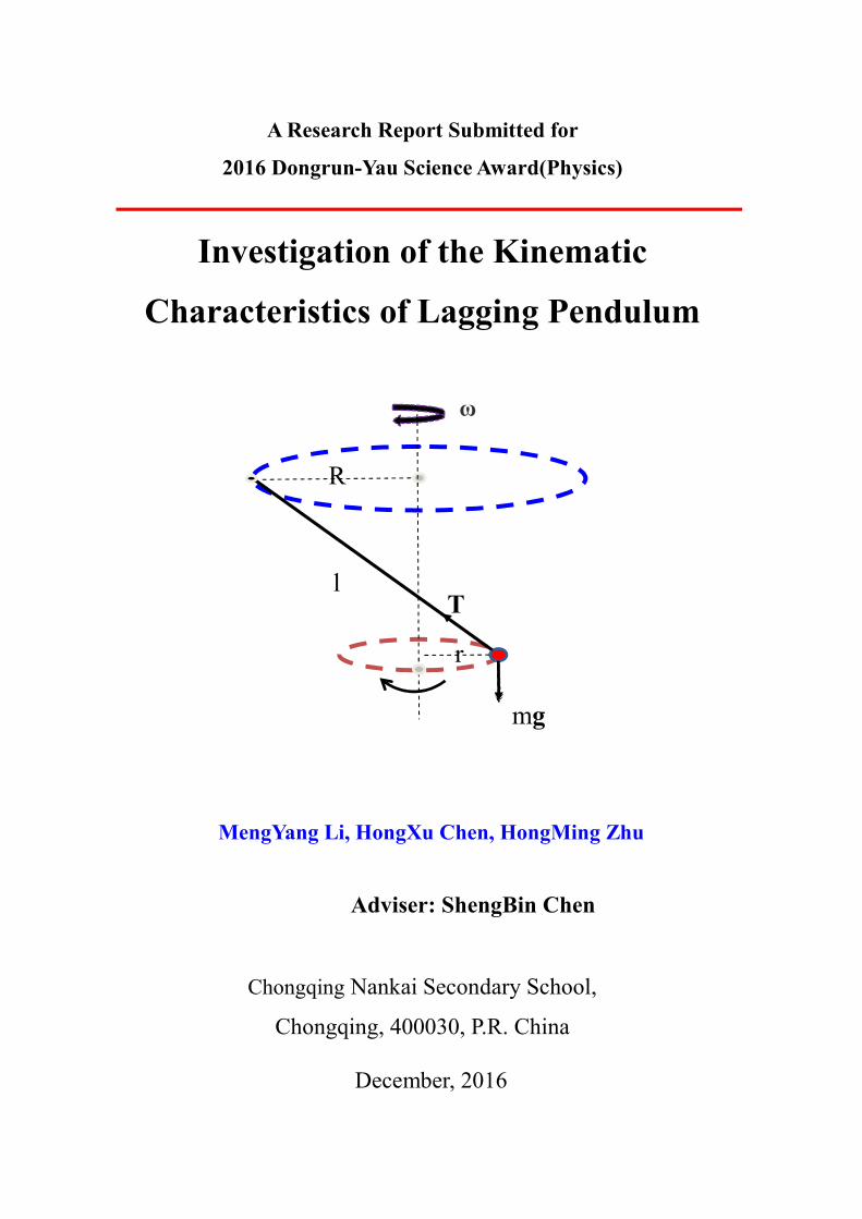
Investigation of the Kinematic

Characteristics of Lagging Pendulum

MengYang Li, HongXu Chen, HongMing Zhu

Adviser: ShengBin Chen

Chongqing Nankai Secondary School,

Chongqing, 400030, P.R. China

December, 2016

R

r

l T

mg

ω

I

Abstract

The pendulum is a historic and important scientific object, fascinating physicists

and becoming one of the paradigms in the study of physics and natural phenomena.

The ordinary simple pendulum and conical pendulum in which the pivot is static and

fixed oscillate regularly and periodically, but a perturbed pendulum with a moving

pivot usually travels chaotic. The kinematic characteristics of the pendulum strongly

depend on the motion behavior of the pivot.

A lagging pendulum is a kind of special perturbed pendulum whose pivot rotates

in a horizontal circle and under certain conditions, the bob traces along a horizontal

circumference with a radius smaller than that of the pivot. By now, the detail

conditions to result in this lagging motion have been still unknown. So in present

work, we investigated the stable motion trajectories of the lagging pendulum and

analyzed the reason to lead to the lagging behavior. By a series of work, such as

preliminary observation, establishing the physical model, solving the motion

equations, developing the calculation programs and performing quantitative

measurement and verification experiments, we obtained the following main results:

1) The experimental observation reveals that the bob travels jerkily and chaotic at

the beginning stage and finally revolves stably. The stable trajectories of the

bob were found to be a horizontal circumference. In the lagging state, the

rotating angular velocity of the bob is equal to that of the pivot, and the

lagging angle is .

2) Based on the results of the preliminary observation, the physical model was

proposed, then the motion equations were established by Newton's second law

and the lowest energy method, respectively. It indicates that when the bob

traces along a circle stably, the radius of the bob, r, is a quartic equation. Its

solution can be obtained when the values of three variables of ω(the angular

velocity of the pivot), R(the radius of the pivot) and l(the length of the string)

are provided.

3) The calculation program developed by C language can work out the radius of

the bob by inputting the values of variables (ω,R,l).The developed

Mathematica programs can intuitively and clearly illustrate the relationship

between the bob radius and two variables of (ω, R, l) in 2D or 3D diagrams.

4) The solution space plots (SSPs) of three particular cases at respectively fixed

II

ω , R and l were obtained. And the characteristics of the solution space and the

lagging zone were discussed and analyzed. It shows that at fixed ω, longer l; at

fixed R or fixed l, higher ω(ω>ωc) will be in favor of the occurrence of

lagging state.

5) The measured radius of the bob is in agreement with the calculated values. The

radius of the bob in the lagging pendulum(r) increases with the radius of the

pivot (R), but deceases with the increase of the rotating angular velocity of the

pivot (ω) or the length of the string (l) when all other variables keep constant.

6) The theoretical analysis and experimental results verified that the motion of the

lagging pendulum is independent of the mass of the bob.

Finally, the features of the ordinary simple pendulum, the conical pendulum, the

carousel pendulum and the lagging pendulum are summarized and discussed briefly.

The above results are beneficial to discover some new phenomena related to the

ordinary pendulum and help us to understand the physical nature of oscillations and

pendulum profoundly. Furthermore, it maybe provide some valuable reference for the

hammer throwers to improve their performance.

Keywords ： Pendulum; Lagging pendulum; Motion equation; Kinematic

characteristics; Solution space plot; Mathematica program.

III

Contents

Abstract .......................................................................................................................... I

Contents .......................................................................................................................III

1. Introduction.............................................................................................................1

2 Preliminary Observation ..........................................................................................4

2.1 Experiment apparatus........................................................................................4

2.2 Results of preliminary observation ...................................................................6

2.3 Chapter summary..............................................................................................8

3 Establishment of Physic Model ...............................................................................9

3.1 Description of the model...................................................................................9

3.2 Assumption of the model and nomenclature.....................................................9

3.3 Establishment of dynamic equation ................................................................10

3.3.1 Based on Newton's second law.............................................................10

3.3.2 Based on the lowest energy method......................................................13

3.4 Preliminary discussion about the motion equation .........................................15

3.5 Chapter summary............................................................................................16

4. Solution and Solution Space of Motion Equations ..................................................17

4.1 Solution of motion equation by C language program.....................................17

4.1.1 The interface of C calculation program ................................................17

4.1.2 The unified motion equation for non-lagging and lagging pendulum ..18

4.1.3 r-ω realtionship and critical ω(ωc)........................................................18

4.2 Solution space plot(SSP) by Mathematica program .......................................20

4.3 Typical results and analysis.............................................................................22

4.3.1 SSPs at fixed angular velocity ..............................................................22

4.3.2 SSPs at fixed pivot radius .....................................................................24

4.3.3 SSPs at fixed string length ....................................................................24

4.3.4 Brief summary of the solution space and the lagging zone ..................26

4.4 Chapter summary............................................................................................27

5 Quantitative Measurement and Verification ..........................................................28

5.1 Experiment goal ..............................................................................................28

5.2 Experiment design ..........................................................................................28

IV

5.3 Experiment results and discussion ..................................................................29

5.3.1 Circular moving trajectories of the bob ................................................29

5.2.2 Measurement results at different pivot radius.......................................29

5.3.3 Discussion of measurement error..........................................................30

5.3.4 Measurement results at different rotating angular velocity ..................31

5.3.5 Measurement results at different string length......................................31

5.3.6 Comparison at different mass of bob ....................................................32

5.3.7 Verification experiment of the lagging and non-lagging zone..............33

5.4 Brief comparison of four ordinary pendulum .................................................34

5.5 Chapter summary............................................................................................34

6 Conclusion and Future Work .................................................................................36

Acknowledgement .......................................................................................................38

Reference .....................................................................................................................38

Appendix......................................................................................................................39

Appendix A. Part of C language calculation program ..........................................39

Appendix B. Part of solution program by Mathematica .......................................43

Appendix C. Some movies of bob's motion .........................................................61

1

1 Introduction

The simple pendulum is of historic and scientific importance [1-5]. Its approximate

isochronisms, first discovered by Galileo Galilee around 1602 , makes it an accurate and

simple timekeeper and, in the hands of Newton, resulted in the first evidence that inertial

and gravitational mass are proportional[5]. The pendulum clock invented by Christian

Huygens( see Fig.1.1) became the world's standard timekeeper, and achieved accuracy of

about one second per year before it was superseded as a time standard by quartz clocks in

the 1930s[1]. And in 1851, Foucault suspended a pendulum from the dome of the Panthéon

in Paris and first demonstrated the Earth's rotation. Now Foucault pendulums (Fig.1.2) are

still displayed in many cities and attract large crowds every year. Besides timekeeper,

pendulums are also used in scientific instruments such as accelerometers and

seismometers [1].

The simple pendulum and conical pendulum are two kinds of ordinary and

conventional pendulum, whose common characteristics is that their supporting point

(pivot) is fixed and static (Fig.1.3). However, when the pivot is forced to move or

oscillate, such as in the perturbed [4], the parametrically-excited [6,11] or the forced

pendulum [7,9,10], the patterns of the motion were found to be complex and chaotic. So the

Fig.1.1 The first pendulum clock built by

Huygens in 1656 [1]

Fig.1.2 Foucault-pendulum: the first demons

-tration of the Earth's rotation (1851) [1]

科

2

simple pendulum became an ideal physical object to study phenomena related to

oscillations, bifurcations and chaos in the framework of nonlinear dynamics [4]. Therefore,

some researcher claimed that rich physics exists in the simple pendulum system [5]. Some

examples of the perturbed pendulum are given in Fig.1.4.

(a) Ordinary simple pendulum [1]

(b) Conical pendulum [2]

Fig. 1.3 Two ordinary pendula in which the supporting point is fixed and static.

(a) Pivot oscillates horizontally . (b) Pivot oscillates vertically .

Fig. 1.4. Some examples of perturbed pendula in which the supporting point moves[4]

(a) the pivot oscillates harmonically in the horizontal direction (b) the pivot oscillates in the vertical

direction(referred as the parametrically excited pendulum).

As shown in Fig.1.5, a lagging pendulum is another kind of special perturbed

pendulum whose pivot travels in a horizontal circle and under certain conditions, the bob

moves along a horizontal circumference with a radius smaller than that of the pivot.

3

However, by now, the information about the lagging pendulum is not so rich and the

detail conditions to result in this lagging motion have been still unknown. The

International Young Physicists' Tournaments' (IYPT) 2016 announced it as a public

question, so in present work, we investigated the motion and stable trajectories of the

lagging pendulum and analyzed the conditions to cause the pendulum to a lagging state.

Our work mainly includes four parts: (1) preliminary observation; (2)

establishment of the physical model and the motion equations; (3) development of two

kinds of calculation programs to get the solution and the solution space; (4) quantitative

measurement and verification experiments.

Fig. 1.5. A lagging pendulum in which the supporting point rotates along a horizontal

circumference and the bob traces a circle with a smaller radius.

4

2 Preliminary Observation

In order to obtain the motion information of the bob and explore whether the bob

travels along a circle with a smaller radius than that of the pivot, a simple experiment

apparatus was first built to perform the preliminary observation.

2.1 Experiment apparatus

The schematic and the practical diagrams of the setup to record the trajectories of the

bob are shown in Fig.2.1. The apparatus mainly consists of a motor, a pivot bar, a string

and a bob. A 42 series stepper motor (MKS BS42HB33-01) was adopted as the driver,

and a 20g counterweight was employed as the bob. A round and hole light PVC bar (1m

long, 1cm in diameter) was applied as the pivot bar. A strong string was tied to the pivot

bar at one end and to the counterweight at the other end. The radius of the pivot (R) can

be adjusted by the place to suspend the bob. As depicted in Fig.2.1.f, the motor, the pivot

bar and a bracket were assembled together, and the assembly rotating part was fixed on

two supports. In order to let the bob fly freely, the supports are at least 2 meters higher

than the ground.

The electronic components (transformer, stepper motor, controlling board and driver

boards) and the electronic circuit to carry out the rotating motion were shown in Fig.2.2.

An electronic fan was added in our experiment to improve the heat radiation of the

stepper driver boards.

Before the measurement, the time for the motor to rotate 100 circles was recorded by

a stopwatch timer, and then the period(T) was calculated and the rotating angular velocity

was determined by ω=2 /T. The motor rotates at a constant speed during the

experimental process. Usually the bob travels chaotic at the beginning of the motion, so it

is very difficult to acquire the track of the bob. When the bob orbits stably, its moving

trail of the bob was recorded by a video camera. According to the ratio of the actual size

to that one in the camera, the x and y-direction moving distance of the bob can be

obtained, then the trajectories of the bob can be analyzed and the radius of the bob(r) can

be worked out.

5

Fig.2.1 The schematic and actual apparatus to measure the motion of the bob

Fig.2.2 The electronic components and circuit for the rotating of the experiment

(d) Electric circuit for the stepper motor

Controller Board Driver Board

Stepper

Transformer

(a) Transformer (b) Controller board (c) DRV8825 driver boards and fan

(c) 42 series stepper motor (d) PVC pivot bar (e) Bracket (f) Assembly of motor and rotator

(a) The schematic set-up (b) The practical set-up

6

2.2 Results of preliminary observation

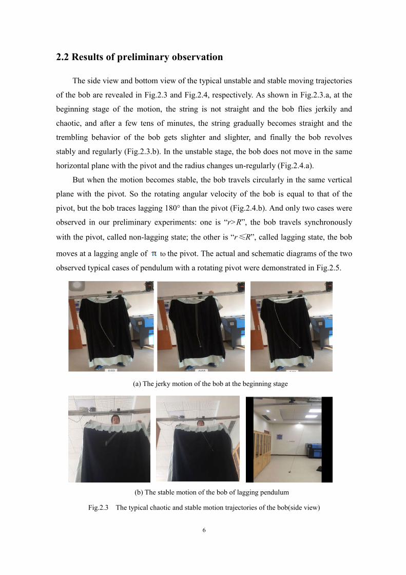
The side view and bottom view of the typical unstable and stable moving trajectories

of the bob are revealed in Fig.2.3 and Fig.2.4, respectively. As shown in Fig.2.3.a, at the

beginning stage of the motion, the string is not straight and the bob flies jerkily and

chaotic, and after a few tens of minutes, the string gradually becomes straight and the

trembling behavior of the bob gets slighter and slighter, and finally the bob revolves

stably and regularly (Fig.2.3.b). In the unstable stage, the bob does not move in the same

horizontal plane with the pivot and the radius changes un-regularly (Fig.2.4.a).

But when the motion becomes stable, the bob travels circularly in the same vertical

plane with the pivot. So the rotating angular velocity of the bob is equal to that of the

pivot, but the bob traces lagging 180° than the pivot (Fig.2.4.b). And only two cases were

observed in our preliminary experiments: one is “r>R”, the bob travels synchronously

with the pivot, called non-lagging state; the other is “r≤R”, called lagging state, the bob

moves at a lagging angle of to the pivot. The actual and schematic diagrams of the two

observed typical cases of pendulum with a rotating pivot were demonstrated in Fig.2.5.

Fig.2.3 The typical chaotic and stable motion trajectories of the bob(side view)

(a) The jerky motion of the bob at the beginning stage

(b) The stable motion of the bob of lagging pendulum

7

Fig.2.4 The typical chaotic and stable motion trajectories of the bob(bottom view)

Fig.2.5 The schematic of the two observed typical cases of pendulum with a rotating pivot

(a) The chaotic and unstable motion at the beginning stage

(b) The stable motion of the bob

≈

(a) Actual non-lagging pendulum (b) Schematic non-lagging pendulum (c) The carousel pendulum

(d) Actual lagging pendulum (e) Schematic lagging pendulum

8

A similar case to the non-lagging pendulum is the carousel pendulum[11].. As shown

in Fig.2.5.c, the carousel pendulum is an ordinary one in which the pivot rotates circularly

and the length of the pendulum is much shorter than the radius R(l<<R), so the bob

synchronously revolves with the carousel.

2.3 Chapter summary

(1)The preliminary experiments show that the bob travels chaotic at the beginning stage

and finally moves stably. The stable trajectories of the bob were verified to be a

horizontal circumference. Two typical motions of the bob were observed: one is

non-lagging pendulum similar to the ordinary carousel pendulum; the other is the lagging

pendulum.

(2) In the lagging state, the radius of the bob(r) is smaller than that of the pivot(R), the

rotating angular velocity of the bob is equal to that of the pivot, and the lagging angle is

.

9

3 Establishment of Physic Model

3.1 Description of the model

Based on the results of the preliminary observation, a model of a lagging pendulum

consisting of a pivot, a strong thread and a bob is shown in Fig.3.1. The bob has mass m and

is suspended by a string of length l .When the pivot of the pendulum starts to travels at a

constant speed ω in a horizontal circle of radius R, under certain conditions, the bob

revolves stably along a horizontal circumference with a radius r smaller than that of the

pivot (R).

(a) Physical model (b) Coordinate systems

Fig.3.1. Physical model and coordinate systems of a lagging pendulum.

3.2 Assumption of the model and nomenclature

Before the detail discussion, we assume:

1. The bob is simplified as a mass point in the model.

2. The string mass is negligible.

3. The deformation of the string is negligible, and the string length l is equal to the sum

of the actual length of the string and the radius of the bob, and remains same in the whole

process.

10

4. Neglecting the effect of air drag or resistance on the pivot bar, the string and the bob.

5. Neglecting effect of friction in transitional parts.

The nomenclature in this work is denoted in following:

ω: Rotational angular velocity of the pivot point (rad/s);

R: Radius of the horizontal circle of the pivot (m);

l: Length of the string (m);

m: Mass of the bob (Kg);

θ: The angle between the string and the vertical direction when the bob has a stable

trajectories (°) ;

r: Radius of the horizontal circle of the bob when it has stable trajectories(m);

g: Gravity acceleration (9.81m/s2);

3.3 Establishment of dynamic equation

Two methods were tried: one is based on Newton's second law from the viewpoint of

force analysis, while the other is on account of the lowest energy method from the

perspective of energy.

3.3.1 Based on Newton's second law

In order to investigate the motion of the bob, are shown in Fig.3.1.b, two spatial

rectangular coordinate systems based on the ground were built: one is o-xyz in which the

bob is in the horizontal plane of o-xy, and the other is o'-x'y'z' in which the origin is the

centre of the circle(o') of the pivot.

There are two forces acting on the bob:

(1) The tension T in the string, which is exerted along the line of the string and acts

toward the point of suspension.

(2) The downward bob weight mg, where m is the mass of the bob and g is the

local gravitational acceleration.

In physics, Newton's laws of motion describe the motion of an object in an inertial

(non-accelerating) frame of reference, while the Coriolis force is an inertial force (also

called a fictitious force) that acts on objects that are in motion relative to a rotating

reference frame. In this work, although the pivot is rotating, the motion of the bob is

relative to the ground, not to the pivot, i.e., the Earth is considered as our inertial frame of

reference, is not a rotating reference frame. Since the Coriolis force exists only when one

uses a rotating reference frame, thus no Coriolis force needs to consider in our case.

11

When the bob stably moves in a horizontal plane, the vertical component of the tension

in the upward direction is balanced to the weight of the bob. If the tension T has a force

component in the horizontal tangential direction along the circumference, there will exist

acceleration in this direction, which would cause the bob travel faster and faster. In this

case, the bob can not move stably. So no force component in the horizontal tangential

direction along the circumference exists, means, when the bob rotates in a horizontal

plane stably, only a centripetal force and gravity, no horizontal transverse force

tangentially, exerts on the bob, so the tension T and gravity must be in the same vertical

plane, and the center of the cycle orbit of the bob and that of the pivot are on the same

vertical line, and their rotating angular velocity are equal.

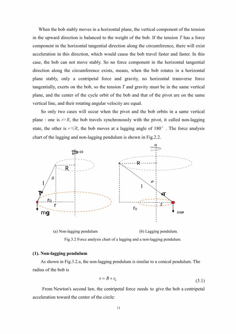
So only two cases will occur when the pivot and the bob orbits in a same vertical

plane : one is r>R, the bob travels synchronously with the pivot, it called non-lagging

state, the other is r≤R, the bob moves at a lagging angle of 180°. The force analysis

chart of the lagging and non-lagging pendulum is shown in Fig.2.2.

(a) Non-lagging pendulum (b) Lagging pendulum.

Fig.3.2 Force analysis chart of a lagging and a non-lagging pendulum.

(1). Non-lagging pendulum

As shown in Fig.3.2.a, the non-lagging pendulum is similar to a conical pendulum. The

radius of the bob is

0r R r (3.1)

From Newton's second law, the centripetal force needs to give the bob a centripetal

acceleration toward the center of the circle:

ω

R

l

T

mg

r0 r

R

r

l

T

mg r0

12

20( )F m r R

(3.2)

The force exerted by the string can be resolved into a horizontal component, T sinθ,

toward the center of the circle, and a vertical component, T cosθ, in the upward direction,

so

F = Tsinθ = mrω2 (3.3)

Since there is no acceleration in the vertical direction, the vertical component of the

tension in the string is equal and opposite to the weight of the bob:

Tcosθ = mg (3.4)

Eliminating T and m from Eq.(3.3) and Eq.(3.4 ), we can obtain:

2sin r cosg (3.5)

Using the trigonometric identity sin(θ)=r0/l, and cosθ=(1-sinθ2)1/2, then

2

20 02

r 1r r

gl l (3.6)

2 4 2 2 2

0 0( ) r ( )gr l r (3.7)

Substituting Eq. (3.1) into Eq. (3.7), yields a formula

4 4 4 3 4 2 2 2 2 2 2r 2( )r [ ( ) ]r 2( ) ( ) 0R R l g Rg r gR

(3.8)

This is the motion equation for non-lagging pendulum.

(2). Lagging pendulum

As shown in Fig.3.2.b, in the lagging pendulum,

0r r R (3.9)

From Newton's second law, the centripetal force is

20( )F m r R

(3.10)

By an analysis procedure similar to the above for the non-lagging pendulum, we

can get

F = Tsinθ = mrω2 (3.11)

Tcosθ = mg (3.12)

Then

2sin r cosg (3.13)

Using the trigonometric identity

sin(θ)=r0/l, and cosθ=(1-sinθ2)1/2 (3.14)

Then

13

220 0

2r 1

r rg

l l

(3.13)

2 4 2 2 20 0( ) r ( )gr l r

(3.14)

Substituting Eq.(3.9) into the above equation, yields an expression

4 4 4 3 4 2 2 2 2 2 2r 2( )r [ ( ) ]r 2( ) ( ) 0R R l g Rg r gR (3.15)

Since r=R can only occur in the lagging state, so from Eq.(3.15)，we have

4 4 4 2 2 2 24 4 0r r l g r (3.16)

If r≠0, then

2 4 2 2 2( 4 ) / 4r l g (3.17)

Thus

2 2 /g l (3.18)

4 2 24 / 2r l g (r=R) (3.19)

Eq.(3.15) is the motion equation for a lagging pendulum(r<R), and Eq.(3.19) is the

result for the special case r=R.

3.3.2 Based on the lowest energy method

From the viewpoint of energy, when the pendulum moves stably, it must be a state

with the lowest energy. So it deserves to study the relation between the energy and the

motion of the pendulum.

The energy of the pendulum is the sum of the kinetic energy and the potential energy.

Before our discussion, we first define that the gravitational potential energy of the rotating

horizontal surface of the pivot is zero.

(1). Non-lagging pendulum

The energy of the non-lagging pendulum shown in Fig.3.2.a is

2 2 2 21( )

2U mr mg l r R

(3.20)

The first and second order partial derivative of U to r is

2

2 2

( )

( )

U mg r Rm r

r l r R

(3.21)

14

322 2 2 2 2

2

Um mgl l r R

r

(3.22)

When the pendulum moves stably and gets equilibrium, it has

0U

r

(3.23)

Then

2

2 2

( )0

( )

mg r Rm r

l r R

(3.24)

Thus

4 4 4 3 4 2 2 2 2 2 2r 2( )r [ ( ) ]r 2( ) ( ) 0R R l g Rg r gR (3.25)

(2). Lagging pendulum

By a similar process, we can obtain the motion equation for lagging pendulum. The

energy of the lagging pendulum shown in Fig.3.2.b is

2 2 2 21( )

2U mr mg l r R

(3.26)

The first and second order partial derivative of U to r is

2

2 2

( )

( )

U mg r Rm r

r l r R

(3.27)

322 2 2 2 2

2

Um mgl l r R

r

(3.28)

If we let

0U

r

(3.29)

Then

2

2 2

( )0

( )

mg r Rm r

l r R

(3.30)

Thus we can get

4 4 4 3 4 2 2 2 2 2 2r 2( )r [ ( ) ]r 2( ) ( ) 0R R l g Rg r gR (3.31)

15

3.4 Preliminary discussion about the motion equation

By comparing Eq.(3.8),Eq.(3.15) with Eq.(3.25) and Eq.(3.31) respectively，we can

find that the Eq.(3.8) is equal to Eq.(3.25), and Eq.(3.25) is same as Eq.(3.31). It means

that the motion equations obtained by Newton's second law and the lowest energy

method are identical.

Therefore, the constraint condition "r>R" or "r≤R" is respectively added to

Eq.(3.25) and Eq.(3.31), thus

For non-lagging state, the motion equation is

4 4 4 3 4 2 2 2 2 2 2r 2( )r [ ( ) ]r 2( ) ( ) 0R R l g Rg r gR

r R

(3.32)

For lagging state, the motion equation is

4 4 4 3 4 2 2 2 2 2 2

2 2 2

r 2( )r [ ( ) ]r 2( ) ( ) 0 )

4 / 2 )

R R l g Rg r gR r R

r l g r R

(3.33)

From the above Eq.(3.32) and Eq.(3.33) , we can obtain that :

(1) There is no parameter m in the two equations, indicating that the motion of the

pendulum has nothing to do with the mass of the bob.

(2) The two equations are both a quartic equation of r, so it is not easy to get the analytical

solutions manually.

(3) Besides the dependent variable r, there are three arguments (ω, R, l) and one

constant(g= 9.81g.cm-2) in the two equations, indicating that r is a function of (ω, R, l)，

i.e.，r = f (ω, R, l), and r can be obtained when the values of (ω, R, l) are available.

But if we want to show the solution of r in a three dimensional (3D) cubic graph, we

have to keep the value of one of (ω, R, l) parameters as the constant, and only two of (ω,

R, l) parameters as the arguments and r as the production, thus the solution becomes the

following forms of functions:

r=f(R,l), ω is fixed (3.34)

r=f(ω,l), R is fixed (3.35)

r=f(ω,R), l is fixed (3.36)

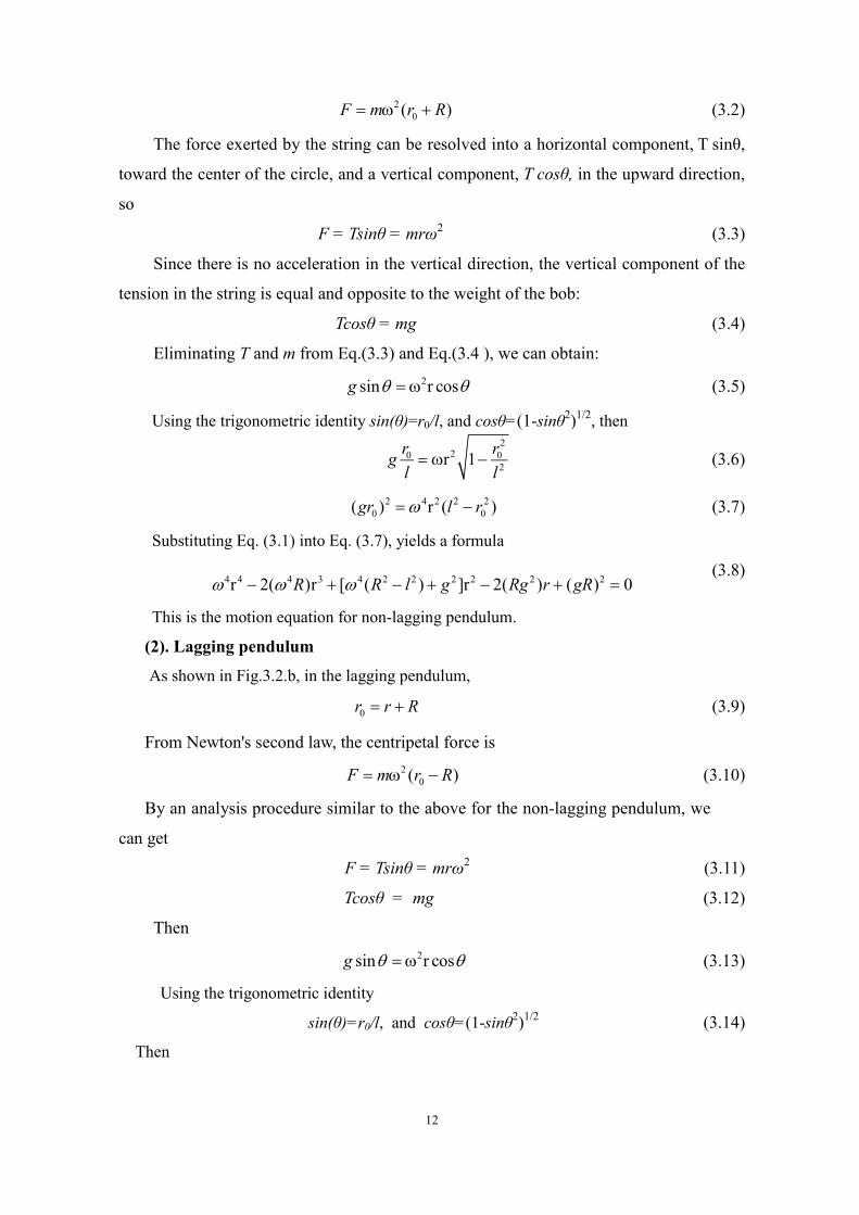
(4) In order to get some intuitive information of solution, we solved Eq.(3.33) for lagging

16

state by setting some special parameters: ω=6.28rad/s, R=0.3m, l=1.0m, g=9.81m/s2, four

roots were obtained: r1= -1.282m; r2= -0.61m; r3=0.113m; r4= 0.630m. Since r is the

radius of the circle, it must be positive, so only r3=0.113m and r4=0.630m are valid from

the perspective of physical significance. Since r3=0.113m<R=0.3m, and r4= 0.630m >

R=0.3m, and Eq.(3.33) is obtained from the initial constraint condition(r<R), so only

r3=0.113m is the actual solution of r.

(5) If R decrease to zero at non-lagging state, the pendulum will become an ordinary

conical pendulum. So we can check whether our equations are right as follows. At R=0,

Eq.(3.32) and Eq.(3.33) will become as

4 4 4 2 2 2r ( )r 0l g (3.37)

If 2r 0 , then

4 2 2 2(r ) 0l g (3.38)

4 2 2 2 2 2 2=g /(l ) g /(l cos )r (3.39)

2 =g/(l cos ) , g/(l cos )

(3.40)

2 / l cos /T g (3.41)

Eq.(3.41) is exactly the period formula for an ordinary conical pendulum, so it is

proved that our equation (E.3.32) is right.

3.5 Chapter summary

1). A physical model was established to describe the lagging and non-lagging pendulum,

and the motion equations were respectively obtained by the Newton's second law and the

lowest energy principle, and the equations obtained by these two methods are identical.

2). The motion equations for lagging and non-lagging are both a quartic equation of r, so

it is not easy to get the analytical solution manually. And the equations indicate that the

motion of the pendulum is independent of the mass of the bob.

(3) The solution of r can be obtained when the values of three variables (ω, R, l) are

available.

17

4 Solution and Solution Space of Motion Equations

4.1 Solution of motion equation by C language program

4.1.1 The interface of C calculation program

Due to the motion equation for the lagging pendulum(Eq.(3.33)) being a quartic

equation, it is difficult to get the analytical solution manually, so we first implemented a

program by C language to calculate the radius of the bob, in which the values of variables

(ω, R, l) are the input and four values of r are the output, among which usually two of

them are minus, being regarded as invalid data since the radius of the circle should be

positive from the perspective of physical significance.

A typical interface of the calculation program is exhibited in Fig.4.1. It inputs:

ω=5.146rad/s, R=0.095m, l=1.5m, and the output roots are: 1.35m, 0.031m, -0.02m and

-1.55m. It is obvious that the latter two minus numbers are invalid, and 1.35m or 0.03m is

probably the solution. Based on the initial constraint condition r<R, so only r=0.03m

(r<R=0.095m) is the exact result.

The main C program is given in Appendix A.

Fig.4.1 The interface of calculation program by C language

18

4.1.2 The unified motion equation for non-lagging and lagging

pendulum

By carefully comparing the motion equation for non-lagging pendulum (Eq.(3.32))

with that for lagging pendulum(Eq.3.33), we found that only the sign of positive and

negative for the odd order of term r, i.e., r and r3 are different in these two equations, so if

we define the r for lagging and non-lagging pendulum are positive and negative

respectively, as shown in Fig.4.2, Eq.(3.32) and Eq.(3.33) can be unified to one equation

as follows,

4 4 4 3 4 2 2 2 2 2 2r 2( )r [ ( ) ]r 2( ) ( ) 0R R l g Rg r gR (4.1)

where r>0 is for the lagging pendulum and r<0 is for the non-lagging one, respectively.

Thus, based on Eq.(4.1), we can use only one time of calculation to acquire the

solution of r for both the non-lagging and the lagging pendulum, the only difference is

that the positive root r(r>0) is for lagging pendulum, but the negative root (r<0) is for

non-lagging.

Fig.4.2 The definition of positive and negative r for lagging and non-lagging pendulum

4.1.3 r-ω relationship and critical ω(ωc)

If we change the values of ω, we can get a series of roots by the above C calculation

program. According to the calculated values of r, we can analyze the relation between the

19

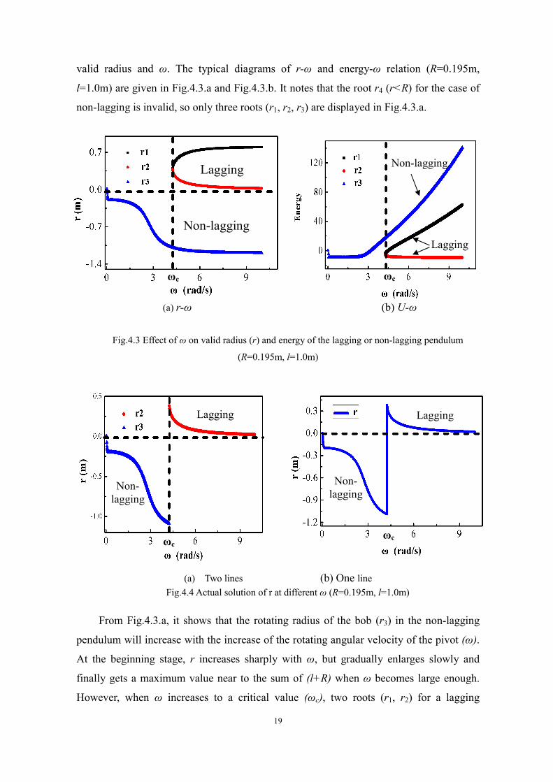
valid radius and ω. The typical diagrams of r-ω and energy-ω relation (R=0.195m,

l=1.0m) are given in Fig.4.3.a and Fig.4.3.b. It notes that the root r4 (r<R) for the case of

non-lagging is invalid, so only three roots (r1, r2, r3) are displayed in Fig.4.3.a.

Fig.4.3 Effect of ω on valid radius (r) and energy of the lagging or non-lagging pendulum

(R=0.195m, l=1.0m)

(a) Two lines (b) One line

Fig.4.4 Actual solution of r at different ω (R=0.195m, l=1.0m)

From Fig.4.3.a, it shows that the rotating radius of the bob (r3) in the non-lagging

pendulum will increase with the increase of the rotating angular velocity of the pivot (ω).

At the beginning stage, r increases sharply with ω, but gradually enlarges slowly and

finally gets a maximum value near to the sum of (l+R) when ω becomes large enough.

However, when ω increases to a critical value (ωc), two roots (r1, r2) for a lagging

Lagging

Non-lagging

(a) r-ω (b) U-ω

Non-lagging

Lagging

ωc ωc

Lagging

Non- lagging

Non- lagging

Lagging

ωc ωc

20

pendulum will occur.

The energy U-ω relation is given in Fig.4.3.b. It reveals that the energy of the

non-lagging pendulum increase with ω. At small ω, the energy of non-lagging pendulum

is lower, so it is in non-lagging state; but when ω is larger than ωc, the energy of lagging

pendulum is lower than that of the non-lagging one, so the pendulum becomes into a

lagging one. Two values of r occur in the lagging state, but the one with lower energy (red

line, r2) will be the actual solution. The actual solution of r at different ω is displayed in

Fig.4.4. It indicates that a non-lagging pendulum happens at ω<ωc, while a lagging

pendulum occur at ω>ωc , and r of lagging pendulum deceases with ω.

So now we can understand how the lagging state happens: when the pivot rotates

slower, the bob will try to catch up its pace with the pivot by flying outside(r>R), but

when the pivot rotates faster and faster, the bob gradually flies behind the pivot. And

when the rotating angular velocity of the pivot (ω) increases to a critical value, the bob

can not keep pace with the pivot anymore, so the bob becomes total lagging , then the

lagging pendulum happens.

4.2 Solution space plot(SSP) by Mathematica program

The calculation program by C language can only give one result at every

combination values of (ω, R, l) parameters. In order to obtain more information about the

distribution of solution intuitively, the dynamic cubic graph of the solution is essential. A

solution space plot (SSP) is such a diagram which can graphically depict the distribution

of the bob radius at steady state when two or more parameters of the system are varied.

So in this work, Wolfram Mathematica 9 software was applied to calculate and draw these

plots. Such plots were obtained by keeping one of (ω, R, l) parameter as the constant, and

setting two of (ω, R, l) parameters as the variables and r as the production. If the 3D SSPs

are planar projected, two dimensional (2D) plane diagrams can be obtained respectively

from the front, above or side view. These 2D diagrams can demonstrate the domain of the

variables.

Furthermore, in order to judge in which zones of variables the pendulum will

become into a lagging state, the plane "r=R" are added in the above 3D SSPs. According

to the aforementioned criterion that r≤R or r>R will be the initial judge condition to

distinguish the lagging or non-lagging state, so a lagging or a non-lagging pendulum will

occur at the zone below or above the plane "r=R" in SSPs, respectively. Thus we can get

21

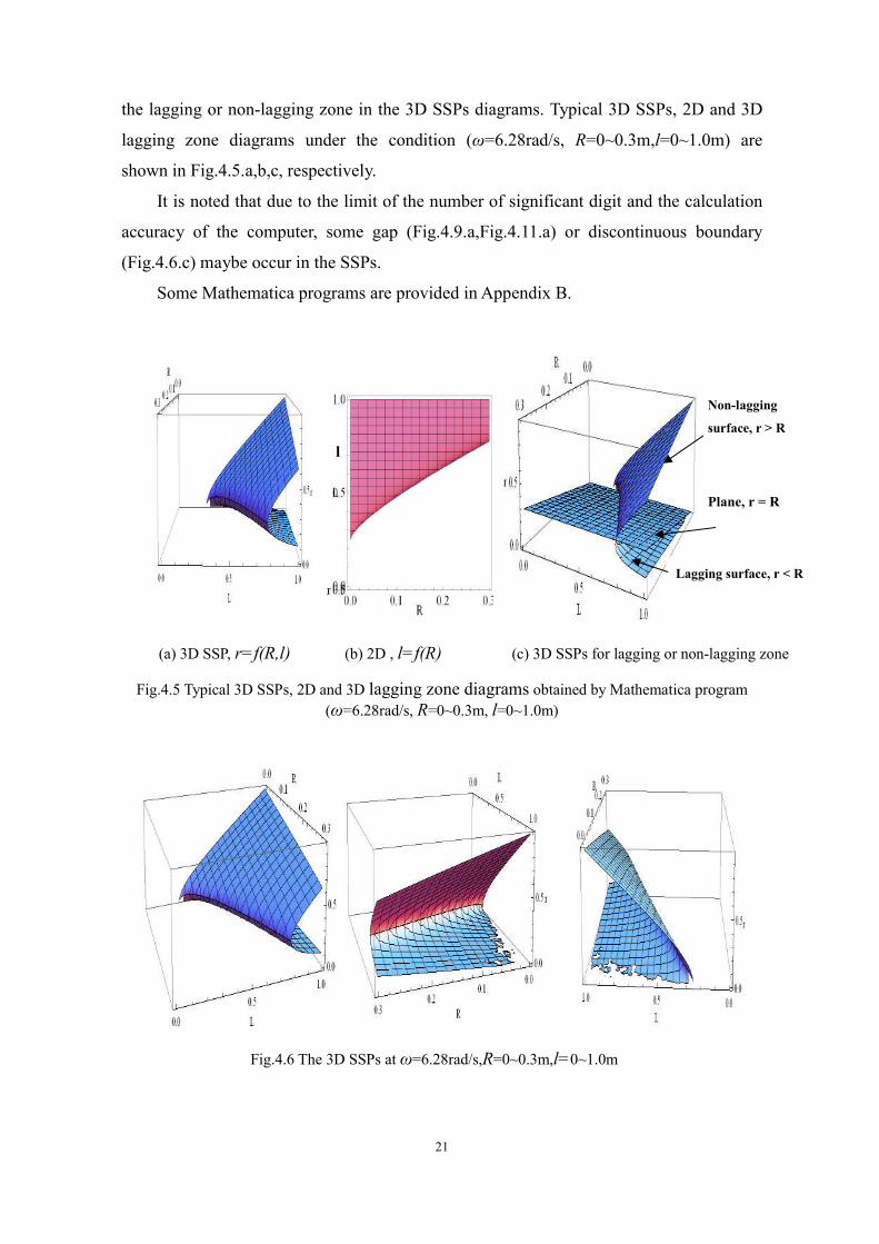
the lagging or non-lagging zone in the 3D SSPs diagrams. Typical 3D SSPs, 2D and 3D

lagging zone diagrams under the condition (ω=6.28rad/s, R=0~0.3m,l=0~1.0m) are

shown in Fig.4.5.a,b,c, respectively.

It is noted that due to the limit of the number of significant digit and the calculation

accuracy of the computer, some gap (Fig.4.9.a,Fig.4.11.a) or discontinuous boundary

(Fig.4.6.c) maybe occur in the SSPs.

Some Mathematica programs are provided in Appendix B.

(a) 3D SSP, r=f(R,l) (b) 2D , l=f(R) (c) 3D SSPs for lagging or non-lagging zone

l

Plane, r = R

Non-lagging

surface, r > R

Lagging surface, r < R

Fig.4.5 Typical 3D SSPs, 2D and 3D lagging zone diagrams obtained by Mathematica program

(ω=6.28rad/s, R=0~0.3m, l=0~1.0m)

Fig.4.6 The 3D SSPs at ω=6.28rad/s,R=0~0.3m,l=0~1.0m

22

4.3 Typical results and analysis

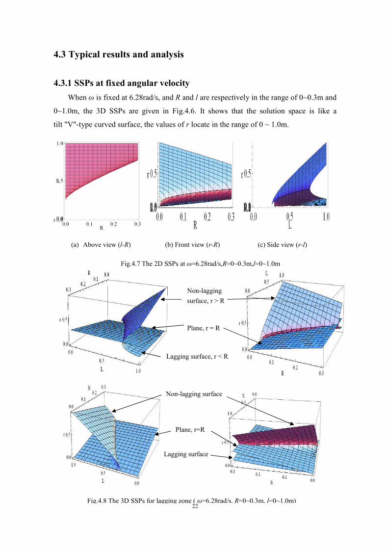
4.3.1 SSPs at fixed angular velocity

When ω is fixed at 6.28rad/s, and R and l are respectively in the range of 0~0.3m and

0~1.0m, the 3D SSPs are given in Fig.4.6. It shows that the solution space is like a

tilt "V"-type curved surface, the values of r locate in the range of 0 ~ 1.0m.

(a) Above view (l-R) (b) Front view (r-R) (c) Side view (r-l)

Fig.4.7 The 2D SSPs at ω=6.28rad/s,R=0~0.3m,l=0~1.0m

Plane, r=R

Non-lagging surface

Lagging surface

Plane, r = R

Non-lagging

surface, r > R

Lagging surface, r < R

Fig.4.8 The 3D SSPs for lagging zone ( ω=6.28rad/s, R=0~0.3m, l=0~1.0m)

23

The corresponding 2D SSPs are illustrated in Fig.4.7. It reveals that r only occurs at

the zone with l larger than 0.25m, means, the string length must be larger than a critical

value lc which increases with the pivot radius (Fig.4.7.a). It indicates that a long string is

essential to obtain the valid motion of the pendulum.

For the case of ω=6.28rad/s, R=0~0.3m, l=0~1.0m, the lagging or non-lagging

parameters surface is revealed in Fig.4.8. It is obvious that the lagging states mainly occur

in the zone of l> lc and r<R.

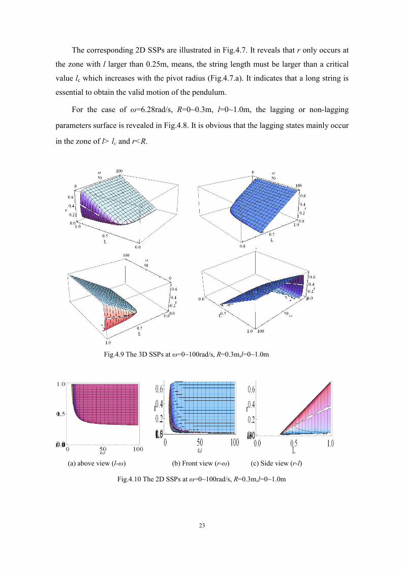
(a) above view (l-ω) (b) Front view (r-ω) (c) Side view (r-l)

Fig.4.9 The 3D SSPs at ω=0~100rad/s, R=0.3m,l=0~1.0m

Fig.4.10 The 2D SSPs at ω=0~100rad/s, R=0.3m,l=0~1.0m

24

4.3.2 SSPs at fixed pivot radius

The 3D SSPs for the case that R is fixed at 0.3m, and ω and l are respectively in the

range of 0~100 rad/s and 0~1.0m are depicted in Fig.4.9. It shows that the solution space

is like an "L"-type curved surface, the values of r are in the range of 0 ~ 1.0m.

The 2D SSPs are exhibited in Fig.4.10. It reveals that r mainly occurs at the zone of

the string longer than about 30cm and the angular velocity of the pivot larger than about

4.5 rad/s, means, l> lc and ω>ωc are needed. It implies that a long string and a large

angular velocity are essential to acquire the valid motion of the pendulum.

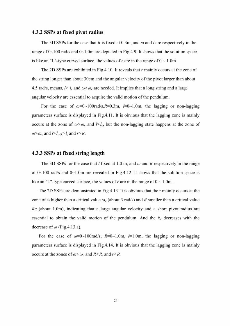
For the case of ω=0~100rad/s,R=0.3m, l=0~1.0m, the lagging or non-lagging

parameters surface is displayed in Fig.4.11. It is obvious that the lagging zone is mainly

occurs at the zone of ω>ωc and l>lc, but the non-lagging state happens at the zone of

ω>ωc and l>lr=R>lc and r>R.

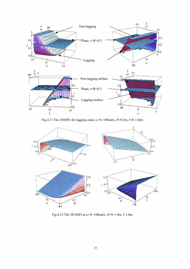
4.3.3 SSPs at fixed string length

The 3D SSPs for the case that l fixed at 1.0 m, and ω and R respectively in the range

of 0~100 rad/s and 0~1.0m are revealed in Fig.4.12. It shows that the solution space is

like an "L"-type curved surface, the values of r are in the range of 0 ~ 1.0m.

The 2D SSPs are demonstrated in Fig.4.13. It is obvious that the r mainly occurs at the

zone of ω higher than a critical value ωc (about 3 rad/s) and R smaller than a critical value

Rc (about 1.0m), indicating that a large angular velocity and a short pivot radius are

essential to obtain the valid motion of the pendulum. And the Rc decreases with the

decrease of ω (Fig.4.13.a).

For the case of ω=0~100rad/s, R=0~1.0m, l=1.0m, the lagging or non-lagging

parameters surface is displayed in Fig.4.14. It is obvious that the lagging zone is mainly

occurs at the zones of ω>ωc and R<Rc and r<R.

25

Plane, r=R=0.3

Non-lagging

Lagging

Plane, r=R=0.3

Non-lagging surface

Lagging surface

Fig.4.11 The 3DSSPs for lagging zone( ω=0~100rad/s, R=0.3m, l=0~1.0m)

Fig.4.12 The 3D SSPs at ω=0~100rad/s, R=0~1.0m, l=1.0m

26

Fig.4.13 The 2D SSPs at ω=0~100rad/s,R=0~1.0m, l=1.0m

Fig.4.14 The 3D SSPs for lagging zone (ω=0~100rad/s, R=0~1.0m, l=1.0m)

4.3.4 Brief summary of the solution space and the lagging zone

In this section, the SSPs of three particular cases, each at a fixed value of ω , R and l,

respectively, were obtained and the lagging or non-lagging zone were discussed and

Plane, r=R

Non-lagging surface

Lagging surface

Plane, r=R

Non-lagging surface

Lagging surface

(a) Abovel view (R-ω) (b) Front view (r-ω) (c) Side view (r-R)

27

analyzed. The shape of solution space and the characteristics of lagging or non-lagging

zone are summarized in Table 4.1. It indicates that at fixed ω, longer l; at fixed R or fixed

l, higher ω will be in favor of the occurrence of lagging state.

Table 4.1 Summary of the characteristics of the solution space and the lagging zone

Case Constant Variables Shape of SSP

Valid range of variables

Lagging Zone Non-Lagging Zone

1 ω=6.28ad/s R=0~1.0m, l=0 ~ 1.0m

V l>lc； lc inc.vs R

l>lc and r<R l>lc and r>R

2 R=0.3m ω=0~100rad/s, l=0~1.0m

L ω>ωc and l>lc；lc dec.vs ω

ω>ωc and l>lc and r<R

ω>ωc and l>lr=R>lc and r>R

3 l=1.0m ω=0~100rad/s, R=0~1.0m,

L ω>ωc and R<Rc, Rc inc. vs ω

ω>ωc and R<Rc

and r<R

ω>ωc and R<Rr=R <Rc

and r>R

Note: subscript ”c” : “critical”; inc:increase; dec:decrease.

4.4 Chapter summary

(1) The calculation program developed by C language can calculate the radius of the bob

by inputting the values of the variables (ω, R, l) .

(2) A non-lagging pendulum happens at ω<ωc, while a lagging pendulum occurs at ω>ωc ,

and the r of lagging pendulum deceases with the increase of ω.

(3) The developed Mathematica programs can clearly and intuitively illustrate the

relationship between the bob radius and two variables of (ω, R, l) in 3D or 2D graphs.

(4) The SSPs of three particular cases of respectively fixing the values of ω , R and l were

obtained. And the characteristics of the solution space and the lagging zone were

discussed and analyzed. It is found that at fixed ω, longer l; at fixed R or fixed l, higher ω

will be in favor of the occurrence of lagging state.

28

5 Quantitative Measurement and Verification

5.1 Experiment goal

In chapter two, we have get some qualitative results that under certain parameters,

the lagging pendulum will travel in a circle with the radius of the bob(r) smaller than that

of the pivot(R), the rotating angular velocity of the bob is equal to that of the pivot, and

the lagging angle is . But the detail relationship of r and the angular velocity, the length

of the string and the pivot radius are still unknown. So in present work, the quantitative

measurement experiments were designed to achieve the following goals:

1) To get the stable motion trajectories of the bob and judge whether the bob travels

in circle or not, and if it moves circularly, work out the radius of the bob, and then

compare the measured and calculated results;

2) To verify the exact motion state of the bob at the calculated lagging zone or

no-lagging zone;

3) To verify whether the motion of the pendulum has relevance to the mass of the

bob.

5.2 Experiment design

Since the trajectories of the bob is related to the angular velocity, the length of the

string and the pivot radius, so each group of the experiments were done by keeping one of

the variables of (ω, R, l) as a constant, and varying two of them. For example, when ω is

fixed, the values of R and l were changed. In this work, five series of experiments are

designed:

(1) Different ω: ω=0~8rad/s, R=0.195m, l=1.00m.

(2) Different R: R=0~0.3m，ω=5.145rad.s-1; l=1.50m.

(3) Different l: l=0~1.50m,ω=6.28rad/s, R=0.195m.

(4) Different mass of the bob: 20g and 50g.

(5) Verification experiment of the lagging and non-lagging zone.

For each group of experiment parameter, 3 times of experiment were done, and the

average value was taken as the measured result.

29

5.3 Experiment results and discussion

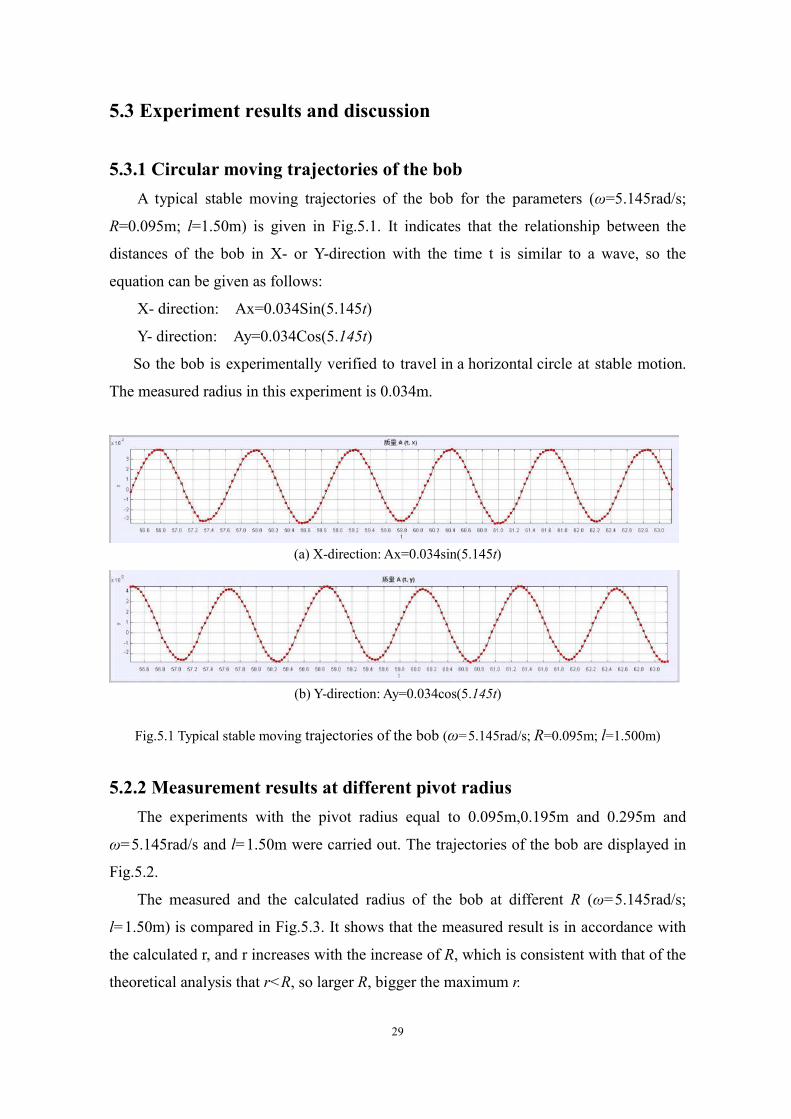
5.3.1 Circular moving trajectories of the bob

A typical stable moving trajectories of the bob for the parameters (ω=5.145rad/s;

R=0.095m; l=1.50m) is given in Fig.5.1. It indicates that the relationship between the

distances of the bob in X- or Y-direction with the time t is similar to a wave, so the

equation can be given as follows:

X- direction: Ax=0.034Sin(5.145t)

Y- direction: Ay=0.034Cos(5.145t)

So the bob is experimentally verified to travel in a horizontal circle at stable motion.

The measured radius in this experiment is 0.034m.

(a) X-direction: Ax=0.034sin(5.145t)

(b) Y-direction: Ay=0.034cos(5.145t)

Fig.5.1 Typical stable moving trajectories of the bob (ω=5.145rad/s; R=0.095m; l=1.500m)

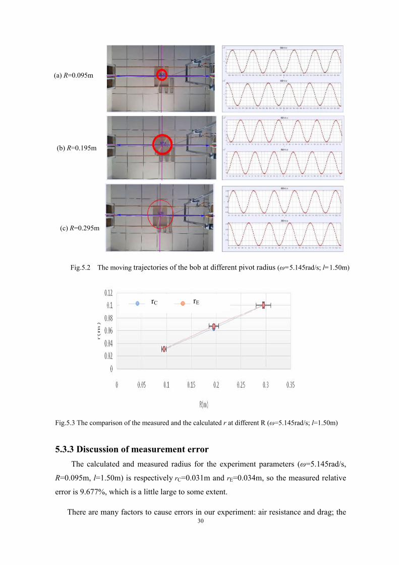
5.2.2 Measurement results at different pivot radius

The experiments with the pivot radius equal to 0.095m,0.195m and 0.295m and

ω=5.145rad/s and l=1.50m were carried out. The trajectories of the bob are displayed in

Fig.5.2.

The measured and the calculated radius of the bob at different R (ω=5.145rad/s;

l=1.50m) is compared in Fig.5.3. It shows that the measured result is in accordance with

the calculated r, and r increases with the increase of R, which is consistent with that of the

theoretical analysis that r<R, so larger R, bigger the maximum r.

30

Fig.5.3 The comparison of the measured and the calculated r at different R (ω=5.145rad/s; l=1.50m)

5.3.3 Discussion of measurement error

The calculated and measured radius for the experiment parameters (ω=5.145rad/s,

R=0.095m, l=1.50m) is respectively rC=0.031m and rE=0.034m, so the measured relative

error is 9.677%, which is a little large to some extent.

There are many factors to cause errors in our experiment: air resistance and drag; the

(a) R=0.095m

(b) R=0.195m

(c) R=0.295m

Fig.5.2 The moving trajectories of the bob at different pivot radius (ω=5.145rad/s; l=1.50m)

rC rE

31

mass of the string; the uneven angular velocity of the pivot; whether the bob moves stably.

Typically, it is worth noting that usually it takes some time( tens of minutes) for the bob

to get into a stable motion, but it is not easy to manually judge whether the bob travels

stably or not, so if one records the trajectories of the bob before its stable motion, a very

large measured error yields.

Here we briefly discuss the error caused by considering the bob as a mass point. The

counterweight actually has a height of 24cm and a width of 11cm, so it will lead to the

centroid error and the position error, as shown in Fig.5.4. The position error is ⊿rE=1/2 d

cosθ, where d is the width of the counterweight and θ is the tilt angle.

After taking into account for the error of the bob size, new data were gotten,

rC=0.0308m and rE=0.0312m, so the measured error is 1.299%.The relative error in our

experiment is roughly in the range of 1.3%~4.9%.

5.3.4 Measurement results at different rotating angular velocity

The experiments with ω changing from 4.28rad/s to 8.0rad/s and R=0.195m and

l=1.00m, were performed. The measured results are given in Fig.5.5. It reveals that the r

decreases with the increase of ω, which is in accordance with our theoretical study

(Fig.4.10.b and Fig.4.13.b) and the results of J.Zhao et al. that r decreases with the

increase of ω2[12].

5.3.5 Measurement results at different string length

The experiments with the string length of 0.60m~1.50m and ω=6.28 rad/s and

R=0.195m were carried out. The measured results are shown in Fig.5.6. It is obvious that

Centroid error

Position error

Fig.5.4 The error caused by regarding the bob as a mass point

32

the r decreases with the increase of l, which is in agreement with our theoretical analysis

(Fig.4.7.c and Fig.4.10.c) and the results of J.Zhao et al.[12].

5.3.6 Comparison at different mass of bob

To test whether the motion of the pendulum is related to the mass of the bob, two

counterweight, 20g and 50g, were used for comparison. The results at ω=5.146rad/s,

l=1.50m, R= (0.095m, 0.195m, 0.295m) are given in Fig.5.7. It is found that that within

the margin of error, the measured radius of the 20g bob are equal to that of 50g, and the

measured radius are near to the calculated results. So the theoretical deduction that the

motion of the pendulum is independent of its mass was verified by the experiments.

Fig.5.7 The comparison of calculated and measured radius at different mass of the bob

(ω=5.145rad/s; l=1.50m, R=(0.095,0.195, 0.295)m)

rC 20g rE 50g rE

R (m)

Fig.5.5 The comparison of the measured and

calculated r at different ω (R=0.195m; l=1.0m)

Fig.5.6 The comparison of the measured and

calculated r at different l (ω=6.28rad/s; R=0.195m)

ωC

33

5.3.7 Verification experiment of the lagging and non-lagging zone

All of the above experiments were done in the calculated lagging zones, so the

lagging pendulums were actually caught into our sight. In order to examine whether

different moving phenomenon will happen in the non-lagging zones, we choose some

parameters in the non-lagging zones to do some investigation.

The observation results at the angular velocity keeping constant at 5.145rad/s, and

varying the pivot radius and string length are given in Table 5.1 and Fig.5.8. It indicates

that the lagging occurs at r<R, but the non-lagging happens at r>R, which is consistent

with the deduction of the theoretical analysis.

Table 5.1 The observation results at the variables zones of r<R and r>R (ω=5.145rad/s)

Exp No. R(m) l(m) rC(m) rC<R Observed motion

1 0.095 1.50 0.031 Yes Lagging

2 0.195 1.50 0.065 Yes Lagging

3 0.295 1.50 0.102 Yes Lagging

4 0.095 0.80 0.086 Yes Lagging

5 0.195 0.80 0.241 No Non-Lagging

r

R l

(a) 3D solution space, the grey tilt plane is r=R

(b) 2D solution space. "O" and "X" denotes r<R and r>R, respectively.

(d) Non-lagging.

(c) Lagging .

Fig.5.8 The observed different motion state at r<R and r>R zones (ω =5.145 rad/s)

5 4

3 2 1

34

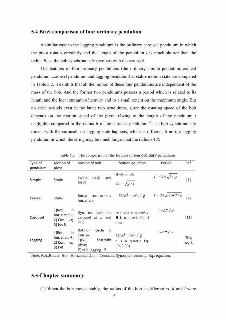
5.4 Brief comparison of four ordinary pendulum

A similar case to the lagging pendulum is the ordinary carousel pendulum in which

the pivot rotates circularly and the length of the pendulum l is much shorter than the

radius R, so the bob synchronously revolves with the carousel.

The features of four ordinary pendulums (the ordinary simple pendulum, conical

pendulum, carousel pendulum and lagging pendulum) at stable motion state are compared

in Table 5.2. It exhibits that all the motion of these four pendulums are independent of the

mass of the bob. And the former two pendulums possess a period which is related to its

length and the local strength of gravity and to a small extent on the maximum angle. But

no strict periods exist in the latter two pendulums, since the rotating speed of the bob

depends on the motion speed of the pivot. Owing to the length of the pendulum l

negligible compared to the radius R of the carousel pendulum[11], its bob synchronously

travels with the carousel, no lagging state happens, which is different from the lagging

pendulum in which the string may be much longer that the radius of R.

Table 5.2 The comparison of the features of four ordinary pendulums

Type of pendulum

Motion of pivot

Motion of bob Motion equation Period Ref.

Simple Static Swing back and forth

θ=θ0sinωt，

/g l

2 /T l g [1]

Conical Static Rot.at con. ω in a hor. circle

2tan /r g 2 cos /T l g

[2]

Carousel

1)Rot. in hor. circle R; 2) Con. ω; 3) l<< R

Syn. rot. with the carousel at ω and r>R

2 2tan / sin /R g l g θ is a quartic Eq.of time

T=2 /ω

[11]

Lagging

1)Rot. in hor. circle R; 2) Con. ω; 3) l>R

Rot.hor. circle r; Con. ω. 1)r>R, Syn.with pivot;

2) r<R, lagging .

2tan /r g r is a quartic Eq.

(Eq.3.33)

T=2 /ω

This work

Note: Rot.:Rotate; Hor.: Horizontal; Con.: Constant; Syn:synchronously; Eq.: equation,

5.5 Chapter summary

(1) When the bob moves stably, the radius of the bob at different ω, R and l were

35

measured and the measured radius is in agreement with the calculated, the relative error is

1.3%~4.9%.

(2) It is found that r increases with R, but deceases with the increase of ω or l at all

other variables keeping constant.

(3) The experiments verified that the motion of the lagging pendulum is independent

of the mass of the bob.

(4) The characteristics of the ordinary simple pendulum, conical pendulum, carousel

pendulum and lagging pendulum are compared and analyzed briefly.

36

6 Conclusion and Future Work

In this work, the stable motion characteristics of a lagging pendulum in which the

pivot moves along a horizontal circumference has been investigated theoretically and

experimentally. And the features of the ordinary simple pendulum, conical pendulum,

carousel pendulum and lagging pendulum are discussed briefly. The following conclusion

can be obtained:

1) The experimental observation reveals that the bob travels chaotic at the beginning

stage and finally moves stably. The stable trajectories of the bob were verified to

be a horizontal circumference. In the lagging state, the rotating angular velocity of

the bob is equal to that of the pivot, and the lagging angle is 180°.

2) The motion equations obtained based on Newton's second law and lowest energy

principle indicates that when the bob moves stably, the radius of the bob, r, is a

quartic equation whose solution can be obtained when the three variables of ω, R

and l are provided.

3) The calculation program developed by C language can work out the radius of the

bob by inputting the values of variables (ω, R, l).The developed Mathematica

programs can clearly and intuitively illustrate the relationship between the bob

radius and two variables of (ω, R, l) in 2D or 3D graphs.

4) The SSPs of three particular cases at the fixed ω, R and l, respectively, were

obtained. And the characteristics of the solution space and the lagging zone were

discussed and analyzed. It shows that at fixed ω, longer l((l/R)ω>(l/R)c)>1); at

fixed R or fixed l, higher ω(ω>ωc) will be in favor of the occurrence of lagging

state.

5) The measured radius of the bob is in agreement with the calculated, the relative

error is 1.3%~4.9%. And r increases with R, deceases with the increase of ω or l

at other variables keeping constant.

6) The theoretical analysis and experimental measurement indicates that the motion

of the lagging pendulum is independent of the mass of the bob.

Although the obtained results for the lagging pendulum are ideal and reasonable, it

can further be improved when following aspects are taken into account:

1) To obtain more information of the solution space. Due to the limited time, only

37

the SSPs of three particular cases, in which ω, R and l and are respectively fixed at a

constant value, were obtained and discussed in present work. In the future, the

relationship between the SSPs and different ω, R and l should be further analyzed.

2) In the future, the unstable trajectories of the bob at the beginning stage can be

chosen as the physical object to study chaos.

Furthermore, our analysis method and some results can provide valuable reference to

the athletes who are engaged in the rotation and throwing events (discus, hammer, shot

and javelin),such as hammer or discus thrower to improve their performance. The goal of

these sports is to release the subject with maximum forward velocity at an appropriate

angle( for the case of shot put, approximately forty degrees is the best). So the thrower

must carefully and elaborately control the relation between the speed, release height,

angle and release point.

In summary, since the first scientific investigation of the pendulum by Galileo about

410 years ago, the pendulum has been a basic and important physical object to study

physics and natural phenomena. The topic related to pendulum seems to be historic and

ancient, but actually a lot of new phenomena, typical those related to oscillations,

bifurcations and chaos in nonlinear system still attract a large number of mathematicians

and physicists. Rich physics exists in the simple pendulum system.

The simple pendulum is still a fascinating and attractive research topic.

Fig.6.1 Our method or results may be beneficial for the hammer throwers to improve the

performance

38

Acknowledgement

We are indebted to our teacher----Mr. ShengBin Chen at Nankai Secondary

School who supervised this work and gave us a lot of good advice. Special thanks

should be given to Mr. Pan Zhang in College of Physics, Chongqing University, who

assisted and supported us in the experiment process. We also thank Chongqing

University and VEX of Nankai Secondary School for lending the experiment

equipment and others who helped us during the study.

Reference

[1]. Wikipedia : Pendulum, https://en.wikipedia.org/wiki/Pendulum

[2]. Wikipedia: Conical pendulum, https://en.wikipedia.org/wiki/Conical_pendulum

[3]. Wikipedia : Angular momentum, https://en.wikipedia.org/ wiki/ Angular_

momentum

[4]. J. L. Trueba, J. P. Baltan, and M. A. F. Sanjuan. A generalized perturbed pendulum.

Chaos, Solitons and Fractals, 15(2003) 911-924

[5]. R. A. Nelson, M. G. Olsson. The pendulum -Rich physics from a simple system.

Am. J. Phys. 54(1986)2

[6]. B. Horton, J. Sieber, J. M. T. Thompson, and M. Wiercigroch. Dynamics of the

nearly parametric pendulum. Int. J. Non-Linear Mech. 46 (2011)2: 436–442

[7]. ， ，D.J.Tritton Ordered and chaotic motion of a forced spherical pendulum Eur. J.

Phys. 7 (1986) 162-169.

[8]. X. Xu, M. Wiercigroch, M.P. Cartmell, Rotating orbits of a parametrically-excited

pendulum,Chaos, Solitons and Fractals 23 (2005) 1537–1548

[9]. J.Mawhin, The forced pendulum: A paradigm for nonlinear analysis and dynamical

systems. Exp Math,6(1998)271–287.

[10]. P.Amster, M. C.Mariani,Some results on the forced pendulum equation,

Nonlinear Analysis 68 (2008) 1874–1880

[11]. A.Vial, An approximate and an analytical solution to the carousel-pendulum

problem, Eur. J. Phys. 30 (2009) L75–L78

[12]. J.Zhao，Q.Zhang，J.Q.Cao, Theoretical derivation and experimental

verification of lagged pendulum’ s stable motion, J.Eastern Liaoning University

( Natural Science)，23(2016) 4:300-395 (in Chinese)

39

Appendix

Two kinds of programs were developed in present work. One is the calculation

program by C language, and the other is the solution program and the drawing program

of solution space plots by Mathematica software.

Some of the programs is list as follows:

Appendix A. Part of C language calculation program

#include <bits/stdc++.h>

#include <complex>

#include <iostream>

#include <math.h>

using namespace std;

void quartic_equation

(

double a,double b,double c,double d,double e,

complex<double> &x1,complex<double> &x2,

complex<double> &x3,complex<double> &x4

);

double check(double w,double R,double l,double r){

double tmp=w*w*r*r;

tmp-=9.81*sqrt(l*l-(r+R)*(r+R));

return tmp;

}

int main()

{

double a,b,c,d,e;

complex<double> x1,x2,x3,x4;

std::cout<<"please input w ,R ,l: (rad/s,m,m)"<<endl;

double wo,R,l;

cin>>wo>>R>>l;

a=wo*wo*wo*wo;

b=2*R*a;

c=9.81*9.81-(l*l-R*R)*a;

40

d=2*R*9.81*9.81;

e=9.81*9.81*R*R;

quartic_equation(a,b,c,d,e,x1,x2,x3,x4);

printf("\nThe possible answers:\n");

double ans,tans=INT_MAX;

if(x1.imag()==0.0)

tans=check(wo,R,l,x1.real()) , ans=x1.real() , printf("x1 = %.2lf

\n",x1.real());;

if(x2.imag()==0.0){

if(tans==check(wo,R,l,x2.real())) printf("!!!!!!");

if(tans>check(wo,R,l,x2.real())) tans=check(wo,R,l,x2.real()) , ans=x2.real();

printf("x2 = %.2lf \n",x2.real());

}

if(x3.imag()==0.0){

// if(tans==check(wo,R,l,x3.real())) printf("!!!!!!");

// if(tans>check(wo,R,l,x3.real())) tans=check(wo,R,l,x3.real()) , ans=x3.real();

printf("x3 = %.2lf \n",x3.real());

}

if(x4.imag()==0.0){

if(tans==check(wo,R,l,x4.real())) printf("!!!!!!");

if(tans>check(wo,R,l,x4.real())) tans=check(wo,R,l,x4.real()) , ans=x4.real();

printf("x4 = %.2lf \n",x4.real());

}

if(ans<0) printf("\nnon-lagging! radius: %.2lf \n",-ans);

else printf("\nlagging! radius: %.2lf \n",ans);

system("pause");

return 0;

}

void quadratic_equation(double a4,double b4,double c4,complex<double>

&z1,complex<double> &z2)

{

double delta;

complex<double> temp1,temp2;

delta=b4*b4-4*a4*c4;

complex<double> temp(delta,0);

temp1 = (-b4)/(2*a4);

temp2 = sqrt(temp)/(2*a4);

z1=temp1+temp2;

41

z2=temp1-temp2;

}

double cubic_equation(double a3,double b3,double c3,double d3)

{

double p,q,delta;

double M,N;

double y0;

complex<double> temp1,temp2;

complex<double> x1,x2,x3;

complex<double> y1,y2;

if(a3==0)

{

quadratic_equation(b3,c3,d3,y1,y2);

x1 = y1;

x2 = y2;

x3 = 0;

}

else

{

p = -1.0/3*pow((b3*1.0/a3),2.0)+c3*1.0/a3;

q = 2.0/27*pow((b3*1.0/a3),3.0)-1.0/3*b3*c3/(a3*a3)+d3*1.0/a3;

delta = pow((q/2.0),2.0)+pow((p/3.0),3.0);

complex<double> omega1(-1.0/2, sqrt(3.0)/2.0);

complex<double> omega2(-1.0/2, -sqrt(3.0)/2.0);

complex<double> yy(b3/(3.0*a3),0.0);

M = -q/2.0;

if(delta<0)

{

N = sqrt(fabs(delta));

complex<double> s1(M,N);

complex<double> s2(M,-N);

x1 = (pow(s1,(1.0/3))+pow(s2,(1.0/3)))-yy;

x2 = (pow(s1,(1.0/3))*omega1+pow(s2,(1.0/3))*omega2)-yy;

x3 = (pow(s1,(1.0/3))*omega2+pow(s2,(1.0/3))*omega1)-yy;

}

else

{

N = sqrt(delta);

complex<double> f1(M+N,0);

42

complex<double> f2(M-N,0);

if(M+N >= 0)

temp1 = pow((f1),1.0/3);

else

temp1 = -norm(pow(sqrt(f1),1.0/3));

if(M-N >= 0)

temp2 = pow((f2),1.0/3);

else

temp2 = -norm(pow(sqrt(f2),1.0/3));

x1 = temp1+temp2-yy;

x2 = omega1*temp1+omega2*temp2-yy;

x3 = omega2*temp1+omega1*temp2-yy;

}

}

y0 = real(x1);

return y0;

}

void quartic_equation

(

double a,double b,double c,double d,double e,

complex<double> &x1,complex<double> &x2,

complex<double> &x3,complex<double> &x4

)

{

double a2,b2,c2;

double a4,b4,c4;

double a3,b3,c3,d3;

double y;

complex<double> y1,y2,y3,y4;

if(b==0 && c==0 && d==0 && e==0)

{

x1 = 0; x2 = 0; x3 = 0; x4 = 0;

}

else if (b==0 && d==0 && e==0)

{

b3 = a; c3 = 0; d3 = c;

quadratic_equation(b3,c3,d3,y1,y2);

x1 = y1; x2 = y2; x3 = 0; x4 = 0;

}

else

43

{

b= b/a; c= c/a; d= d/a; e= e/a; a= a/a;

a3= 8.0;

b3= -4.0*c;

c3= 2.0*b*d-8.0*e;

d3= e*(4.0*c-b*b)-d*d;

y = cubic_equation(a3,b3,c3,d3);

a2= 1.0;

b2= b/2.0-sqrt(8.0*y+b*b-4*c)/2.0;

c2= y-(b*y-d)/sqrt(8.0*y+b*b-4*c);

quadratic_equation(a2,b2,c2,y1,y2);

x1 = y1;

x2 = y2;

a4= 1.0;

b4= b/2.0+sqrt(8.0*y+b*b-4.0*c)/2.0;

c4= y+(b*y-d)/sqrt(8.0*y+b*b-4.0*c);

quadratic_equation(a4,b4,c4,y3,y4);

x3 = y3;

x4 = y4;

}

}

Appendix B. Part of solution program by Mathematica

The Mathematica programs mainly include three parts:

(1) General solution of motion equation of the lagging pendulum;

(2) Special solution of motion equation of the lagging pendulum at one fixed

argument, such as ω, R, or l;

(3) Drawing program of 3D solution space plots

Here we provide the general solution, a special solution at fixed angular velocity

ω=6.28 rad/s and 3 Program to draw Solution Space Plot at (ω=6.28 rad/s, R=0~0.3m,

l=0~1.0m)and “r=R” plane

44

B.1 General Solution of the motion equation of the lagging pendulum Eq. 4.1.

45

46

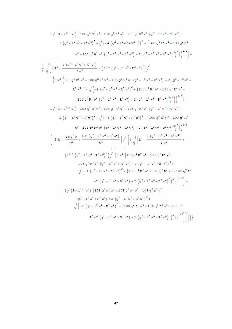
47

48

2 Special Solution of the Eq.4.1 at ω=6.28 rad/s

49

50

51

52

53

54

55

56

57

3 Program to Draw Solution Space Plot at (ω=6.28 rad/s, R=0~0.3m,

l=0~1.0m)and “r=R” plane

58

59

60

61

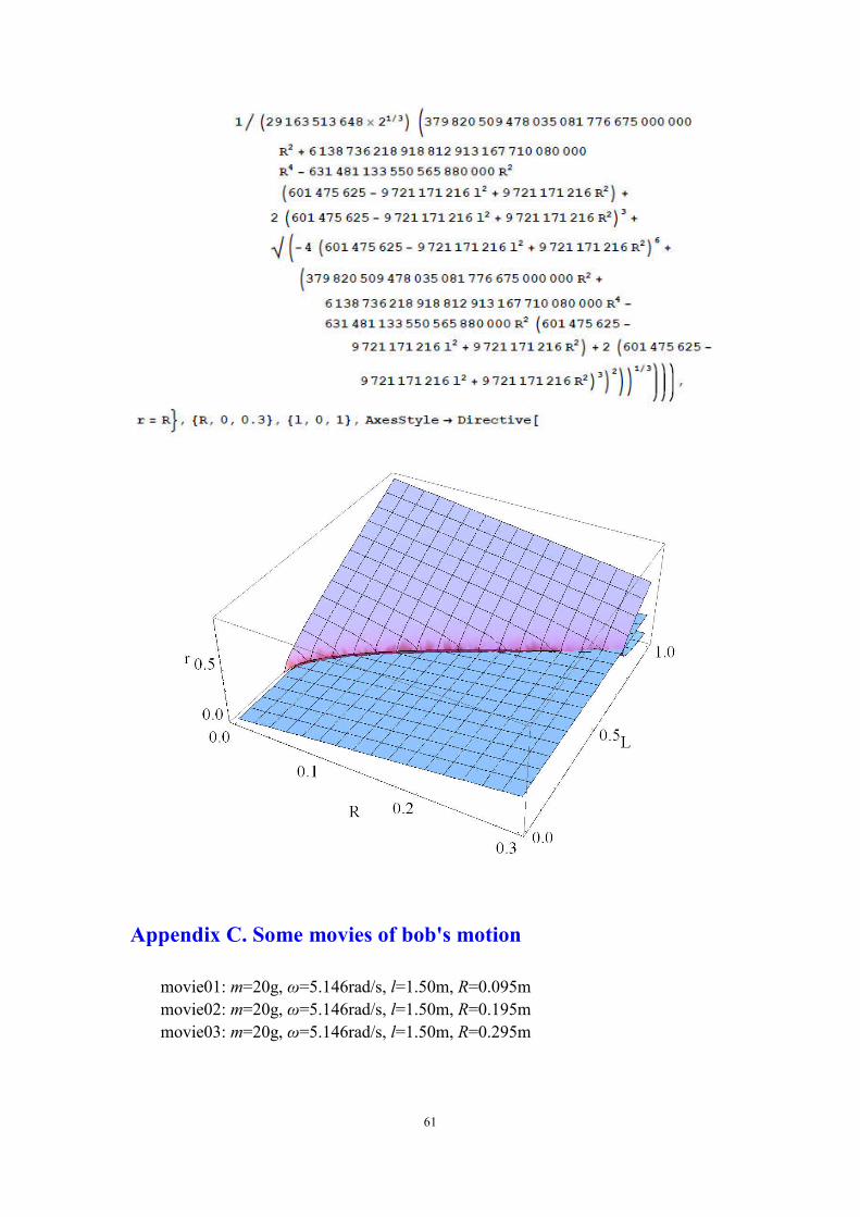
Appendix C. Some movies of bob's motion

movie01: m=20g, ω=5.146rad/s, l=1.50m, R=0.095m

movie02: m=20g, ω=5.146rad/s, l=1.50m, R=0.195m

movie03: m=20g, ω=5.146rad/s, l=1.50m, R=0.295m